Cost Modeling and EstimationFor OLAP-XML Federations

Authors: Dennis PedersenKarsten RiisTorben Bach Pedersen

Technical Report 02-5003Department of Computer Science

Aalborg UniversityCreated on August 14, 2002

Cost Modeling and Estimation For OLAP-XML Federations

Dennis Pedersen Karsten Riis Torben Bach Pedersendennisp@cs.auc.dk riis@cs.auc.dk tbp@cs.auc.dk

Department of Computer Science, Aalborg University

Fredrik Bajers Vej 7E, 9220 Aalborg Ø, Denmark

Abstract

The ever-changing data requirements of today’s dynamic businesses are not handled well by current On-Line Analytical Processing (OLAP) systems. Physical integration of unexpected data into OLAP systemsis a long and time-consuming process, making logical integration, or federation, the better choice in manycases. The increasing use of XML, e.g. in business-to-business (B2B) applications, suggests that the requireddata will often be available in XML format. Thus, federations of OLAP and XML databases will be veryattractive in many situations. However, a naive implementation of OLAP-XML federations will not performwell enough to be useful. In an efficient implementation, cost-based optimization is a must, creating a needfor an effective cost model for OLAP-XML federations. However, existing cost models do not support suchsystems.

In this paper we present a cost model for OLAP-XML federations, along with techniques for estimatingthe cost model parameters in a federated OLAP-XML environment. The paper also present the cost modelsfor the OLAP and XML components in the federation on which the federation cost model is built. Thecost model has been used as the basis for effective cost-based query optimization in OLAP-XML federa-tions. Experiments show that the cost model is precise enough to make a substantial difference in the queryoptimization process.

1 Introduction

OLAP systems [20] enable powerful decision support based on multidimensional analysis of large amountsof detail data. OLAP data are often organized in multidimensional cubes containing measured values that arecharacterized by a number of hierarchical dimensions.

However, dynamic data, such as stock quotes or price lists, is not handled well in current OLAP systems, al-though being able to incorporate such frequently changing data in the decision making-process may sometimesbe vital. Also, OLAP systems lack the necessary flexibility when faced with unanticipated or rapidly changingdata requirements. These problems are due to the fact that physically integrating data can be a complex andtime-consuming process requiring the cube to be rebuilt [20]. Thus, logical, rather than physical, integration isdesirable, i.e. a federated database system [17] is called for. The increasing use of Extended Markup Language(XML)[22], e.g. in B2B applications, suggests that the required external data will often be available in XMLformat. Also, most major DBMSs are now able to publish data as XML. Thus, it is desirable to access XMLdata from an OLAP system, i.e., OLAP-XML federations are needed. For the implementation of OLAP-XMLfederations to perform satisfactorily, cost-based optimization is needed. This, in turn, creates a need for aneffective cost model for OLAP-XML federations. However, existing cost models do not support such systems.

In this paper we present such a cost model for OLAP-XML federations, along with techniques for estimat-ing cost model parameters in an OLAP-XML federation. We also present the cost models for the autonomousOLAP and XML components in the federation on which the federation cost model is based. The cost model hasbeen used as the basis for effective cost-based query optimization in OLAP-XML federations, and experimentsshow that the cost model is powerful enough to make a substantial difference in the query optimization process.

1

A great deal of previous work on data integration exist, e.g., on integrating relational data [7], object-oriented data [16], and semi-structured data [2] However, none of these handle the issues related to OLAPsystems, e.g., dimensions with hierarchies. One paper [15] has considered federating OLAP and object data,but does not consider cost-based query optimization, let alone cost models. To our knowledge, no generalmodels exist for estimating the cost of an OLAP query (MOLAP or ROLAP). Shukla et al. [18] describe howto estimate the size of a multidimensional aggregate, but their focus is on estimating storage requirements ratherthan on the cost of OLAP operations. Also, we know of no cost models for XPath queries, the closest relatedwork being on path expressions in object databases [11]. Detailed cost models have been investigated before forXML [9], relational components [4], federated and multidatabase systems [5, 7, 16, 25, 26], and heterogeneoussystems [3, 10]. However, since our focus is on OLAP and XML data sources only, we can make manyassumptions that permit better estimates to be made. Several techniques have been used in the past for acquiringcost information from federation components. A commonly used technique is query probing [24] where specialqueries, called probing queries, are used to determine cost parameters. Adaptive cost estimation [8] is used toenhance the quality of cost information based on the actual evaluation costs of user queries.

We believe this paper to be the first to propose a cost model for OLAP-XML federation queries, alongwith techniques for estimating and maintaining the necessary statistics. Also, the proposed cost models for theautonomous OLAP and XML components are believed to be novel.

The rest of the paper is organized as follows. Section 2 describes the basic concepts of OLAP-XML fed-erations. Section 3 describes the federation system architecture and outlines the query optimization strategy.Sections 4, 4, 5, and 6 presents the federation cost model and the cost models for the OLAP and XML compo-nents. Section 8 presents a performance study evaluating the cost model. Section 9 summarizes the paper andpoints to future work. Appendices A, B, and C contain additional detail on the OLAP component cost model,the XML component cost model, and the queries performed in the experiments, respectively.

2 OLAP-XML Federation Concepts

This section briefly describes the concepts underlying the OLAP-XML federations that the cost model is aimedat. These concepts are described in detail in another paper [13]. The examples in the paper is based on acase study concerning B2B portals, where a cube tracks the cost and number of units for purchases madeby customer companies. The cube has three dimensions: Electronic Component (EC), Time, and Supplier.External data is found in an XML document that tracks component, unit, and manufacturer information. Thedetails of the case study are also described in [13].

The OLAP data model is defined in terms of a multidimensional cube consisting of a cube name, dimen-sions, and a fact table. Each dimension has a hierarchy of the levels which specify the possible levels of detailof the data. Each level is associated with a set of dimension values. Each dimension also captures the hierarchyof the dimension values, i.e., which values roll up to one another. Dimensions are used to capture the possibleways of grouping data. The actual data that we want to analyze is stored in a fact table. A fact table is a relationcontaining one attribute for each dimension, and one attribute for each measure, which are the properties wewant to aggregate, e.g., the sales price. The cubes can contain irregular dimension hierarchies [12] where thehierarchies are not balanced trees. The data model captures this aspect as it can affect the summarizability ofthe data [12], i.e., whether aggregate computations can be performed without problems. The data model isequipped with a formal algebra, with a selection operator for selecting fact data, ��������� , and a generalized pro-jection operator,

������ , for aggregating fact data. On top of the algebra, a SQL-based OLAP query language,SQL � , has been defined. For example, the SQL � query “SELECT SUM(Quantity),Nation(Supplier) FROMPurchases GROUP BY Nation(Supplier)“ computes the total quantity of the purchases in the cube, grouped bythe Nation level of the Supplier dimension. The OLAP data model, algebra, and the SQL � query language isdescribed in detail in another paper [12].

Extended Markup Language (XML) [22] specifies how documents can be structured using so-called ele-ments that contains attributes with atomic values. Elements can be nested within and contain references to each

2

other. For example, for the example described above, a “Manufacturer” element in the XML document containsthe “MCode” attribute, and is nested within a “Component.” XPath [22] is a simple, but powerful language fornavigating within XML documents. For example, the XPath expression “Manufacturer/@Mcode” selects the“MCode” attribute within the “Manufacturer” element.

The OLAP-XML federations are based on the concept of links which are relations linking dimension valuesin a cube to elements in an XML document, e.g., linking electronic components (ECs) in the cube to the relevant“Component” elements in the XML document. A federation consists of a cube, a collection of XML documents,and the links between the cube and the documents. The most fundamental operator in OLAP-XML federationsis the decoration operator which basically attaches a new dimension to a cube based on values in linked XMLelements. Based on this operator, we have defined an extension of SQL � , called SQL �� , which allows XPathqueries to be added to SQL � queries, allowing linked XML data to be used for decorating, selecting, andgrouping fact data. For example, the SQL �� query “SELECT SUM(Quantity),EC/Manufacturer/@MCodeFROM Purchases GROUP BY EC/Manufacturer/@MCode“ computes total purchase quantities grouped by themanufacturer’s MCode which is found only in the XML document. The OLAP-XML federation concepts aredescribed in detail in another paper [13].

3 The Federation System

In this section we give an overview of the OLAP-XML federation system, the design considerations and opti-mization techniques as well as their use in the federation system.

Temp. Data XML Data

User Interface

XML Comp.Interface

OLAP Comp.Interface

FederationManager

SQLM

SQLXM

SQL SQL

SQLOLAP Query

LanguageXML QueryLanguage

XPath

Meta-data Link Data

OLAP Data

ComponentQuery Evaluator

StatisticsManager

Global CostEvaluator

ComponentCost Evaluator

GlobalOptimizer

QueryDecomposer

Prefetcher

Parser

ExecutionEngine

CacheManager

Federation Manager

Component Interface

SQLxm query

Parsed Query

IntermediateGlobal Plan

XML ComponentPlan

Request

OptimizedGlobal Plan

RequestCost

Request CostExecuteComponent Plan

ExecuteComponent Plan

Update

Requestor Update

ComponentPlan

Request

XML DataAvailable

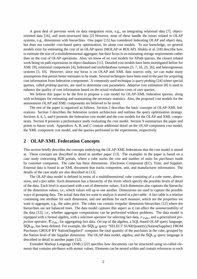
Figure 1: Architecture Of The Federation System and The Federation Manager

The overall architectural design of a prototype system supporting the SQL �� query language is seen tothe left in Figure 1. Besides the OLAP component and the XML components, three auxiliary componentshave been introduced to hold meta data, link data, and temporary data. Generally, current OLAP systemseither do not support irregular dimension hierarchies or it is too expensive to add a new dimension, whichnecessitates the use of a temporary component. SQL �� queries are posed to the Federation Manager, whichcoordinates the execution of queries in the data components using several optimization techniques to improvequery performance. A partial prototype implementation has been performed to allow us to make performanceexperiments. In the prototype, the OLAP component uses Microsoft Analysis Services and is queried withMDX and SQL. The XML component is based on Software AG’s Tamino XML Database system [19], which

3

provides an XPath-like interface. For the external temporary component, a single Oracle 8i system is used.Since the primary bottleneck in the federation will usually be the moving of data from OLAP and XML

components, our optimization efforts have focused on this issue. These efforts include both rule based and costbased optimization techniques, which are based on the transformation rules for the federation algebra. Theoptimization techniques are described in detail in another paper [14].

The rule based optimization uses the heuristic of pushing as much of the query evaluation towards thecomponents as possible. Although not generally valid, this heuristic is always valid in our case since theconsidered operations all reduce the size of the result. The rule based optimization algorithm partitions aSQL �� query tree, meaning that the SQL �� operators are grouped into an OLAP part, an XML part, and arelational part. After partitioning the query tree, it has been identified to which levels the OLAP component canbe aggregated and which selections can be performed in the OLAP component. Furthermore, the partitionedquery tree has a structure that makes it easy to create component queries. The most important cost basedoptimization technique tries to tackle one of the fundamental problems with the idea of evaluating part of thequery in a temporary component: If selections refer to levels not present in the result, too much data needs to betransferred to the temporary component. Our solution to this problem is to inline XML data values into OLAPpredicates as literals. However, this is not always a good idea because, in general, a single query cannot be ofarbitrary length. Hence, more than one query may have to be used. Whether or not XML data should be inlinedinto some OLAP query, is decided by comparing the estimated cost of the alternatives.

The use of cost based optimization requires the estimation of several cost parameters. One of the mainarguments for federated systems is that components can still operate independently from the federation. How-ever, this autonomy also means that little cost information will typically be available to the federation. Hence,providing a good general cost model is exceedingly difficult. In this context, it is especially true for XMLcomponents, because of the wide variety of underlying systems that may be found. Two general techniqueshave been used to deal with these problems: Probing queries, which are used to collect cost information fromcomponents, and adaption, which ensures that this cost information is updated when user queries are posed.

We now outline how the techniques discussed above are used in combination, referring to the componentsseen the right in Figure 1. When a federation query has been parsed, the Query Decomposer partitions theresulting SQL �� query tree, splitting it into three parts: an OLAP query, a relational query, and a number ofXML queries. The XML queries are immediately passed on to the Execution Engine, which determines for eachquery whether the result is obtainable from the cache. If this is not the case, it is sent to the Component QueryEvaluator. The cost estimates are used by the Global Optimizer to pick a good inlining strategy. When theresults of the component queries are available in the temporary component, the relational part of the SQL ��query is evaluated.

4 Federation Cost Model

We now present a basic cost model for OLAP-XML federations. queries, and then outline the optimizationtechniques that, in turn, leads to a refined cost model.

Basic Federation Cost Model: The cost model used in the following is based on time estimates and incorpo-rates both I/O, CPU, and network costs. Because of the differences in data models and the degree of autonomyfor the federation components, the cost is estimated differently for each component. Here, we only present thehigh-level cost model which expresses the total cost of evaluating a federation query. The details of how thesecosts are determined for each component are described later. The OLAP and XML components can be accessedin parallel if no XML data is used in the construction of OLAP queries. The case where XML data is used isdiscussed in the next section. The retrieval of component data is followed by computation of the final result inthe temporary component. Hence, the total time for a federation query is the time for the slowest retrieval ofdata from the OLAP and XML components plus the time for producing the final result. This is expressed in

4

this basic cost formula considering a single OLAP query and � XML queries:

���������������! #"MAX $�%'&)(+*�,.-�%/ ��#(�021�-3334-�% ��#(50 6�798 %�: �<;�=

where %4&)(+*�, is the total time it takes to evaluate the OLAP query, %� ��>(�0 ? is the total time it takes to evaluatethe @ th XML query, and %A: �<;�= is the total time it takes to produce the final result from the intermediate results.

Refined Federation Cost Model: As discussed above, references to level expressions can be inlined in pred-icates thereby improving performance considerably in many cases. Better performance can be achieved whenselection predicates refer to decorations of dimension values at a lower level than the level to which the cube isaggregated. If e.g. a predicate refers to decorations of dimension values at the bottom level of some dimension,large amounts of data may have to be transferred to the temporary component. Inlining level expressions mayalso be a good idea if it results in a more selective predicate.

Level expressions can be inlined compactly into some types of predicates [14]. Even though it is alwayspossible to make this inlining [14], the resulting predicate may sometimes become very long. For predicatessuch as “EC/EC_Link/Manufacturer/MName = Supplier/Sup_Link/SName”, where two level expressions arecompared, this may be the case even for a moderate number of dimension values. However, as long as predicatesdo not compare level expressions to measure values the predicate length will never be more than quadratic in thenumber of dimension values. Furthermore, this is only the case when two level expressions are compared. Forall other types of predicates the length is linear in the number of dimension values [14]. Thus, when predicatesare relatively simple or the number of dimension values is small, this is indeed a practical solution. Very longpredicates may degrade performance, e.g. because parsing the query will be slower. However, a more importantpractical problem that can prevent inlining, is the fact that almost all systems have an upper limit on the lengthof a query. For example, in many systems the maximum length of an SQL query is about 8000 characters.Certain techniques can reduce the length of a predicate. For instance, user defined sets of values (named sets)can be created in MDX and later used in predicates. However, the resulting predicate may still be too long fora single query and not all systems provide such facilities. A more general solution to the problem of very longpredicates is to split a single predicate into several shorter predicates and evaluate these in a number of queries.We refer to these individual queries as partial queries, whereas the single query is called the total query.

Example 4.1 Consider the predicate: “EC/Manufacturer/@MCode = Manufacturer(EC)”. The decoration datafor the level expression results in the following relationships between dimension and decoration values:

EC Manufacturer/@MCodeEC1234 M31EC1234 M33EC1235 M32

Using this table, the predicate can be transformed to: “(Manufacturer(EC) IN (M31, M33) AND EC=’EC1234’)OR (Manufacturer(EC) IN (M32) AND EC=’EC1235’)”. This predicate may be to long to actually be posedand can then be split into: “Manufacturer(EC) IN (M31, M33) AND EC=’EC1234’ ” and “Manufacturer(EC)IN (M32) AND EC=’EC1235’ ”. B

Of course, in general this approach entails a large overhead because of the extra queries. However, sincethe query result may sometimes be reduced by orders of magnitude when inlining level expressions, being ableto do so can be essential in achieving acceptable performance. Because of the typically high cost of performingextra queries, the cost model must be revised to reflect this.

The evaluation time of an OLAP query can be divided into three parts: A constant query overhead that doesnot depend on the particular query being evaluated, the time it takes to evaluate the query, and the time it takesto transfer data across the network, if necessary. The overhead is repeated for each query that is posed, while

5

the transfer time can be assumed not to depend on the number of queries as the total amount of data transferredwill be approximately the same whether a single query or many partial queries are posed. The query evaluationtime will depend e.g. on the aggregation level and selectivity of any selections in a query. How these values aredetermined, is described in Section 5.

The revised cost formula for � XML queries and a single total OLAP query that is split into C partialOLAP queries is presented in the following. The cost formula distinguishes between two types of XML queryresults: Those that have been inlined in some predicate and those that have not been inlined in any predicate.The estimated time it takes to retrieve these results is denoted by %� ��#(�0 D�EF and %� ��#(�0 G9HIFJDKEF , respectively. In theformula let:

L % MAX ��#(�0 G9H�FMDKEF be the maximum time it takes to evaluate some XML query for which the result is not inlinedin any predicate,L % MAX ��#(�0 D�EF be the maximum time it takes to evaluate some XML query for which the result is inlined insome predicate,L % &)(+*�,N0O&)P be the constant overhead of performing OLAP queries,L % ? &)(+*�,N0 QSR ��T be the time it takes to evaluate the @ th partial query,L %'&)(+*�,N0U:V � E � be the time it takes to transfer the result of the total query (or, equivalently, the combinedresult of all partial queries).

Then the cost of a federation query is given by:

�������W"MAX $�% MAX ��#(50 G9H�FMDKEF -�CYX'%'&)(+*�,N0O&)P 8

Z[?U\]1 %

? &)(+*�,^0 Q_R ��T 8 %'&)(+*�,N0U:V � E � 8 % MAX ��>(�0 DKEF 7N8 %4: �`;�=The cost formula is best explained with an example.

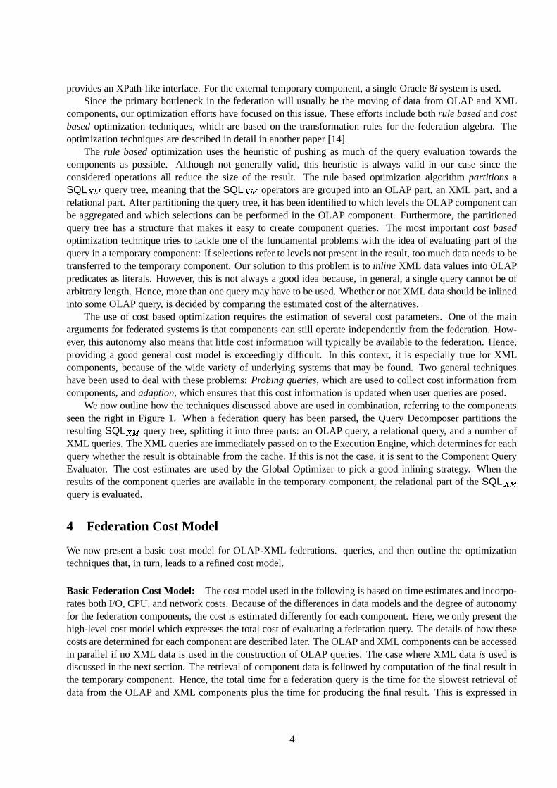
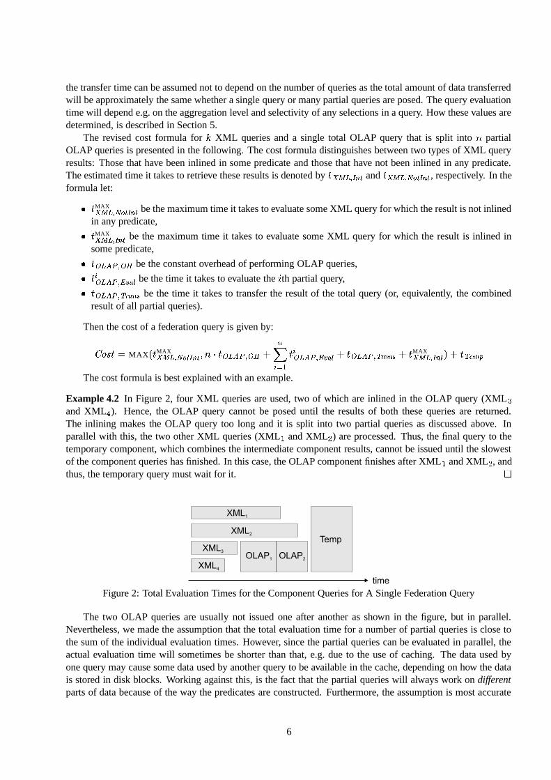
Example 4.2 In Figure 2, four XML queries are used, two of which are inlined in the OLAP query (XML aand XML b ). Hence, the OLAP query cannot be posed until the results of both these queries are returned.The inlining makes the OLAP query too long and it is split into two partial queries as discussed above. Inparallel with this, the two other XML queries (XML 1 and XML c ) are processed. Thus, the final query to thetemporary component, which combines the intermediate component results, cannot be issued until the slowestof the component queries has finished. In this case, the OLAP component finishes after XML 1 and XML c , andthus, the temporary query must wait for it. B

XML1

XML2

XML3

XML4

OLAP1 OLAP2

Temp

time

Figure 2: Total Evaluation Times for the Component Queries for A Single Federation Query

The two OLAP queries are usually not issued one after another as shown in the figure, but in parallel.Nevertheless, we made the assumption that the total evaluation time for a number of partial queries is close tothe sum of the individual evaluation times. However, since the partial queries can be evaluated in parallel, theactual evaluation time will sometimes be shorter than that, e.g. due to the use of caching. The data used byone query may cause some data used by another query to be available in the cache, depending on how the datais stored in disk blocks. Working against this, is the fact that the partial queries will always work on differentparts of data because of the way the predicates are constructed. Furthermore, the assumption is most accurate

6

for OLAP systems running on machines with only a single CPU and disk. For machines with multiple CPUsand disks the maximum evaluation time for any partial query may provide a better estimate. Often the bestgeneral estimate will be somewhere in between, and thus, an average value can be used. Also, the evaluationtime for the total query will sometimes provide a good estimate. It will always take longer than any partialquery, because the partial queries are more selective, and it will generally be faster than the sum of the partialevaluation times, because optimization can be more effective when a single query is used. For example, a fulltable scan may be the fastest way to find the answer to the total query, but by posing several partial queries anumber of index lookups may be used instead. Using the sum of the partial evaluation times will generally besufficiently accurate, because, as is further later, we cannot assume to have detailed cost information available,and consequently, estimates can only be approximate. Which of these estimates is best for a particular OLAPsystem can be specified as a tuning parameter to the federation.

Since any subset of the level expressions can be inlined in the OLAP query, the number of inlining strategiesis exponential in the number of level expressions. None of these can be disregarded simply by looking at thetype of predicate and estimated amount of XML data. Even a large number of OLAP queries each retrievinga small amount of data may be faster than a few queries retrieving most or all of the stored data. Furthercomplicating the issue, is the fact that the choice of whether a particular level expression should be inlined maydepend on which other expressions are inlined. Consider e.g. two predicates that both refer to decorations ofvalues at a low level in the cube, and hence, require the retrieval of a large part of the cube. Inlining only one ofthem may give only a small reduction in the OLAP result size, because the low level values must still be presentin the result to allow the other decoration to be performed. For the same reason, we cannot consider XML dataused for selection independently from XML data that are only used for decoration or grouping. Also, a levelexpression that occurs multiple times in a predicate need not be inlined for all occurrences.

When adding a level expression to the set of inlined expressions, the total cost may increase or it maydecrease. An increase in cost can be caused by two things: The OLAP query may have to wait longer for theextra XML data, or more OLAP queries may be needed to hold the extra data. Any decrease in cost is caused bya reduction in the size of the OLAP result, either because the selectivity of the predicate is reduced or becausea higher level of aggregation is possible. A smaller OLAP result may reduce both the OLAP evaluation timeand the temporary evaluation time.

Component Cost Models: We now describe the models for the component costs that were used in the costformulas in Section 4. This cost information is collected by the Statistics Manager and used by the cost evalua-tors seen to the right in Figure 1. The amount of cost information available to the federation may vary betweenfederation components. Du et al. [3] distinguish between three types of federation components: Proprietary,where all cost information is available to the federation, Conforming, where the component DBMS provides thebasic cost statistics, but not full information about the cost functions used, and finally, Non-Conforming, whereno cost information is available. Usually, only the DBMS vendor has full access to all cost information, andhence, we consider only conforming and non-conforming components here. A high degree of autonomy mustbe expected for XML components, while OLAP components (which are in-house) may or may not provide ac-cess to cost information. Thus, we assume that the OLAP component is either conforming or non-conforming,while the XML components are non-conforming. The temporary component used by the federation is assumedto be a conforming component.

5 OLAP Component Cost Model

As described earlier the cost of an OLAP query comprises a constant query overhead that does not depend onthe particular query being evaluated, the time it takes to actually evaluate the query, and the time it takes totransfer data across the network if necessary:

%�d9e)f�g " %�d9ehf�g 0 dNi 8 % d^ehf�g 0 j9kmlon58 %�d9e)f�g 0 prq�l ZAs7

The statistical information that is needed to estimate these parameters, may be available from the OLAPcomponent’s meta data, in which case it is used directly. However, if such data is not available, we use probingqueries to determine the statistical information and continuously update it by measuring the actual cost of allqueries posed to the components. The probing queries are all relatively inexpensive and can be posed when thesystem load is low, and the overhead of adapting the cost information to the actual costs is insignificant. Hence,these methods introduce little overhead on the federated system.

In the following, we explain how the cost parameters are estimated given an OLAP query by using probingqueries, and how to adapt the cost information when the actual cost of a query is found. We do not explicitlyconsider the use of existing statistical information as this depends very much on the specific DBMS and issimilar to the use of information determined using probing. More specifically, we describe the statistical infor-mation that the estimation is based on and how it is obtained, how the three cost parameters are estimated usingthis information, and how the information is updated.

OLAP Component Statistics The estimation of cost parameters is based on statistical information repre-sented by the functions shown in Table 1.

Function Descriptiontvu ��wW�+xmyzv{A�|{'}~{A� u $|� 7 The rate with which data can be transferred from cube � to the temporarycomponentz����myzv{A�|{'}~{A� u $|� 7 The rate with which data can be read from disk for cube �� u�Ouo� �����'����� $��S-m� 7 The selectivity of predicate � evaluated on cube �� { � ���r�U� u $�� 7 The size of measures �}�� �����_�S� x/{ � ���K�+� $���-m� 7 The relative reduction in size when rolling cube � up to levels ��r�U� u $|� 7 The size of cube �� �+{ �|� ��� u $|� 7 The time for evaluating query �

Table 1: Statistical functions used to determine OLAP cost parameters.

These functions are explained in the following:tvu ��wW�Axoy�z�{��|{'}�{A� u $|� 7 : This function returns the rate with which data can be transferred from cube � to thetemporary component if this is not located on the same server as the OLAP component. This is estimatedby posing a probing query to � . The result is measured in size and timed from when the first resulttuple is received until the last result tuple is received. The data rate can then be approximated from themeasured size and time.z����oy�z�{��|{'}�{A� u $|� 7 : This function returns the rate with which data can be read from disk for cube � . This canbe estimated by posing a probing query that retrieves a part of the base cube and measuring the size of theresult as well as the total query evaluation time:

z����oyzv{A�|{4}�{A� u $|� 7 " � ?O�I�o���N���� K¡�¢/�O£9¤�¤¥�¦ ���! K¡O¢§ ¥`¨�©Iª ��« ¨�¬ § ¥`¨�©oª ��«®­��!¯�°<±K« ¦ ���� K¡O¢ .

By subtracting the constant query overhead and the estimated transfer cost, which will be described later,only the evaluation time is left. The assumption is that a large part of the evaluation time for a query thatretrieves data from the base cube is spent reading the result data from disk. Because indexes are typicallyused to locate such data, little additional data is read from disk.� u��UuI� �����'����� $��_-m� 7 : This function returns the fraction of the total size of � that is selected by � . This is estimatedusing standard methods, i.e. by assuming a uniform distribution, and by considering cardinality, minimumand maximum values of the involved attributes[4]. E.g., if � "³²�´>µ¶·µ�¸>¹ ��º º , where � is a constant, theselectivity of � can be estimated by

� u��UuI� �����4����� $��S-m� 7 " 6 §_» ? Z � e �`km�<n!¤» lo¼+�!n®�`ko��n®¤ §_» ? Z � e �`ko��n®¤ . (Often the smallest/largestbut one is used to ignore extreme values.) If information about cardinality, minimum and maximumvalues is not available, it is obtained by posing probing queries that explicitly request this information.

8

� { � �����O� u $�� 7 : This function returns the size in bytes of a fact containing only values for the measures in � .This is based on the average size of a measure value which is determined from a single probing query.� { � ���r�U� u $|� 7 is used to refer to the size of a fact containing all measures in � .}~� �����r�S� x�{ � ���K�+� $���-m� 7 : This function returns the fraction to which � is reduced in size, when it is rolled up tothe levels � . Shukla et al. [18] propose three different techniques to estimate the size of multidimensionalaggregates without actually computing the aggregates: One is based on the assumption that facts aredistributed uniformly in the cube and does not consider the actual contents of the cube, one performs theaggregation on samples of the cube data and extrapolates to the full cube size, and one scans the entirecube to produce a more precise estimate. Here we use the first method because of its simplicity and speed,and because experimental results in [18] show that it performs well even when facts are distributed rathernon-uniformly.

Using this method, the size of an aggregated result is given by the following standard formula for comput-ing the number of distinct elements ½ obtained when drawing ¾ elements from a multiset of C elements:½ " CÀ¿ÁCW$/Âÿ 1Z 7 q . Given a GP

vÄ Å5Æ 02ÇrÈÉ�OÊˤ�Ì $|� 7 we can then estimate the size of the result lettingC "ÎÍo´ 1>Ï ´ c�ÏÐXXX)Ï ´ 6 Í for all´ ?ÒÑÐ� and ¾ be the number of facts in � , i.e. ¾ " Ó �2Ô � ��£9¤Õ �I F Ó � Ô � �O£9¤ . Hence,ÖØ× ¸�¸<Ù.Ú�Û ¾AÜhÝ�%�@ × CW$���-m� 7 "ßÞq .���O� u $|� 7 : This function returns an estimated size of � , where � may be a cube resulting from an OLAP query,

denoted as � " �à$|� ºU7 . The size of �á$|� ºU7 depends on the selectivity of the predicates included in thequery, and to which levels the cube is rolled up. This leads to the following:

�r�U� u $|�à$|� º 7�7 " âãäãå� u��UuI� �����4����� $��S-m�æº 7 X �r�U� u $|�غ�$|�غ 7�7 if � " �rç $|�غ 7}�� ���<�r�S� x/{ � �����A� $���-m�غ 7 X Õ �I F Ó �2Ô � �OÊË¤Õ �I F Ó �2Ô � �O£9¤ X �r�U� u $|�غK$|�غ 7�7 if � " Ä Å5Æ 02ÇrÈÉ�OÊˤ�Ì $|�æº 7Size of fact table if �à$|�ú 7 is the base cube.

� ��{ �|� ��� u $|� 7 : This function returns the estimated time it takes to evaluate the query � in the OLAP compo-nent. OLAP components often use pre-aggregation to enable fast response times. Hence, the evaluationof a query can be divided into three strategies, the choice of which is determined by which aggregationsare available in the cube. The cost of each of these strategies are discussed in the following. We firstpresent the general formulas that may be used to calculate the evaluation time of an OLAP query, andthen we describe how they are used and when they are applicable.

First, a pre-aggregated result may be available that rolls up to the same levels as the query being evaluated.In that case, the evaluation of the query reduces to a simple lookup. Assuming that proper indexes areavailable on dimension values, any selections referring to dimension values in the aggregated result canbe evaluated using these indexes. This means that the evaluation time of such a query can be assumedto be directly proportional to the combined selectivity of selections in the query and to the size of thepre-aggregated result. However, such a pre-aggregated result can only be used if it is available and if noselection refers to measures in the unaggregated cube or to levels that has been aggregated away in thepre-aggregated result.

If these requirements are not satisfied, the cube may follow a second strategy, in which no pre-aggregatedresults are used. Instead, the query is computed entirely from the base cube. The cost of this computationdepends, of course, on the algorithms implemented in the DBMS, but a simplified cost formula is used,that reflects the evaluation capabilities of many OLAP databases. As above, we assume that selectionscan be evaluated efficiently by use of proper indexing. Hence, any selections in the query that refers tolevels in the cube can be evaluated while accessing the cube, such that only facts that satisfy the selectionpredicates are read from disk. Let this data amount be denoted by ½ . Any selections that refer to measuresin the unaggregated cube can be evaluated at the same time, but these cannot be assumed to make use

9

of indexes. Let the resulting amount of data be denoted by ½Sº . A widely used method of performingaggregation is hashing [6] and we assume that a simple hashing strategy is used. Hence, ½ º bytes of datais partitioned using a hash function and written to disk. Each partition is then read, while aggregation aswell as any selections referring to the aggregated values are performed on the fly. Hence, ½ 8éè ½ º bytesare read from disk to produce the final result.

A third strategy can be used when no selections refer to measures in the unaggregated cube, but one ormore selections may refer to levels that are not present in the aggregated result. In that case the firststrategy cannot be used. However, any pre-aggregated result can still be used as long as it allows allselections that do not refer to measures in the aggregated result to be evaluated. Further aggregation mustbe performed as described for the second strategy to produce the final aggregated result. Hence, the samecost formula can be used, but now the initial cube is instead pre-aggregated and no selections refer tomeasures. Hence, ½hº " ½ and ê+½ bytes are read.

These strategies are summarized in the following formula for the evaluation time of an OLAP query.Assume that queries are on the form �á$|� 7 "ìë cA$ Ä ÅhÆ ÇrÈÉ��Êˤ�Ì $ ë 1'$|� 7�7�7 , where

ë ? denotes a sequence

on selections. Let í Å "ïî 6ð \]1 í µ�¸Kµ Ý�%�@ ¶ @`%<ñ9$�� ð -m� 7 , where selection predicates Â+-3334-o� refer to levels in� , and let í^Ê " î nð \]1 í µ'¸�µ Ý�%<@ ¶ @|%�ñ�$�� ð -m� 7 , where selection predicates Â+-333'- ¸ appear inë 1 and refer to

measures in � . We use the abbreviationzòzæ}

forz����myzv{A�|{'}~{A� u

.

� ��{ �|� ��� u $|�à$|� 7�7 "

âããããããããããããããããäããããããããããããããããå

óôóôÖ $|� 7 § 1 X�½ where ½ " í Å X+íÉ@`õ µ $ �Ä ÅhÆ ÇrÈÉ��ÊˤKÌ $|� 7�7if no selections in

ë 1 refer to measures or levels not in Ä ÅhÆ ÇrÈÉ��ÊˤKÌ $|� 7 ,

and Ä ÅhÆ ÇrÈÉ��ÊˤKÌ is pre-aggregatedóôóôÖ $|� 7 § 1 X5$�½ 8Áè ½�º 7 where ½ " í Å X�íÉ@<õ µ $|� 7 and ½5º " í Ê X4½

if any selections inë 1 refer to measuresóôóôÖ $|� 7 § 1 X'ê+½ where ½ " í Å X4íÉ@`õ µ $ Ä Å)ö®Æ ÇrÈÉ��Êˤ�Ì $|� 7�7

for�Ä ÅhÆ ÇrÈÉ��ÊˤKÌ $|� 7�÷ �Ä ÅhÆ ÇrÈÉ�OÊˤ�Ì $ �Ä Å)öJÆ ÇrÈÉ�OÊ ö ¤KÌ $|�á$|� 7�7�7

if no selections inë 1 refer to measures, or to levels

not invÄ ÅhöMÆ ÇrÈÉ��Ê ö ¤�Ì $|� 7 , and

�Ä Å)ö2Æ ÇrÈÉ��Ê ö ¤�Ì is pre-aggregated

The problem with this formula is that, if a non-conforming component is used, it is not possible to knowwhich results are pre-aggregated and which are not. Hence, we cannot always distinguish between fullyand partially pre-aggregated results, and for partially pre-aggregated results we cannot know which resultsare used. To handle this problem, we use an adaptive approach based on the actual costs of performing theOLAP query. Still, an initial guess is made at the level of pre-aggregation used to evaluate a query. Thiscould be based on the pessimistic assumption that no pre-aggregated results are present in the cube andthus, get a cost that is likely to be too high. Alternatively, it could be based on the optimistic assumptionthat the optimal pre-aggregated result is available and get a cost that is likely to be too low. However,it is not possible to say which of these are best, even for a specific purpose such as deciding whetheror not to inline XML data as discussed earlier. The reason for this is, that no simple relationship existsbetween ø ¶ Ü ¸�ù @|ú µ

and the amount of inlining performed. Whether a low estimate for ø ¶ Ü ¸�ù @|ú µwill

cause more or less XML data to be inlined depends e.g. on the size and selectivities of predicates and thecost of performing computation in the temporary component. Hence, no simple guidelines can be givenas to whether it is better to use an optimistic or a pessimistic estimate of ø ¶ Ü ¸�ù @|ú µ

. Instead, a level ofpre-aggregation is chosen between the bottom and top level of each dimension and this choice is thenimproved by moving up or down in the dimensions as the actual cost of the query is measured. If theactual cost is larger than the estimate, too high a level of pre-aggregation is assumed and vice versa. Thisadaptive technique is explained in more detail later.

10

Estimating and maintaining OLAP cost parameters: The estimation and maintenance of the OLAP costparameters is performed using probing queries as the OLAP component is assumed to be non-conforming. Theinitial estimations are gradually adjusted based on the actual evaluation times using an adaptive approach. Dueto space constraints, we cannot give the details here, they can be found in Appendix A.

6 XML Component Cost Model

Estimating cost for XML components is exceedingly difficult because little or nothing can be assumed aboutthe underlying data source, i.e. XML components are non-conforming. An XML data source may be a simpletext file used with an XPath engine, a relational or OO database or a specialized XML database [19]. The queryoptimization techniques used by these systems range from none at all to highly optimized. Optimizations aretypically based on sophisticated indexing and cost analysis [9]. Hence, it is impossible, e.g., to estimate theamount of disk I/O required to evaluate a query, and consequently, only a rough cost estimate can be made.Providing a good cost model under these conditions is not the focus of this paper and hence, we describe onlya simple cost model.

The cost model is primarily used to determine whether or not XML data should be inlined into OLAPqueries. Hence, in general a pessimistic estimate is better than an optimistic, because the latter may cause XMLdata not to be inlined. This could result in a very long running OLAP query being accepted, simply because itis not estimated to take longer than the XML query. However, the actual cost will never be significantly largerthan the false estimate. Making a pessimistic estimate will not cause this problem although it may sometimesincrease the cost because XML data is retrieved before OLAP data instead of retrieving it concurrently. Forthat reason, conservative estimates are preferred in the model.

The model presented here is based on estimating the amount of data returned by a query, and assuminga constant data rate when retrieving data from the component. Similar to the cost formula for OLAP queries,we distinguish between the constant overhead of performing a query % ��#(�0O&)P and the time it takes to actuallyprocess the query %I ��#(�0 ,_V�H : %� ��#( " %� ��#(�0O&)P 8 %� ��>(�0 ,_V�H Hence, only the latter depends on the size of the result.

In the following we describe how to estimate these two cost parameters given an XPath query. Althoughother more powerful languages may be used, the estimation technique can easily be changed to reflect this. Forsimplicity we consider only a subset of the XPath language where XPath expressions are on the form describedin [14]. Because XML components are non-conforming, the estimates are based on posing probing queries tothe XML component to retrieve the necessary statistics.

XML Component Statistics: Estimation of the cost parameters %� ��#(�0O&)P and %� ��#(�0 ,_V�H is based on thestatistical information described in the following. The way this information is obtained and used to calculatethe cost parameters is described later. In the descriptions û is the name of a node, e.g. the element node“Supplier” or the attribute node “NoOfUnits”, while ø denotes the name of an element node. Let

Ú Üh%/ü j�ý be asimple XPath expression on the form þ�øv1�þ�ø�c'þæ333�þ�ø Z , that specifies a single direct path from the root to a setof element nodes at some level C without applying any predicates.

t ��ÿ u �r�U� u $ Ú Üh%/ürj 7 : The average size in bytes of the nodes pointed to by� {A��� Q . The size of a node is the total

size of all its children, if any.� {+�����S� $ � {���� Q ° 7 : The average number of ø Z elements pointed to by each of its parent elements ø Z § 1 . Noticethat there may be ø Z elements that are children of other elements, since there can be several paths to thesame type of element. The fanout is estimated for each of these paths.

11

� u��UuI� �����'����� $�� 7 : The selectivity of predicate � in its given context. For simplicity, two types of predicates aredistinguished: Simple predicates and complex predicates. Simple predicates are on the form �>1�����c ,where each ��? is either a node with a numeric content or a numeric constant and � is a comparisonoperator. The selectivity of these predicates are estimated from the maximum and minimum values asdescribed for OLAP queries. All other predicates are complex and may refer to non-numeric nodes andvarious functions, e.g. for string manipulation. (An exception is predicates involving the

Ú ×�� @|%�@ × CW$ 7function, which is estimated as a simple predicate.) Following previous work [1], the selectivity ofcomplex predicates is set to a constant value of 10%.��{Ax/ÿ+����{ � ����� $ � {A��� Q ° 7 : The total number of elements pointed to by

� {A��� Q ° . The cardinality of ø Z can becalculated from any ancestor element ø 6 along the path using this formula:

��{+x/ÿA����{ � ����� $ Ú Ü5%�ü_j�ý 7 " ��{+x/ÿA����{ � ����� $ Ú Ü5%�ü_j 7 XZ�

?O\�6 �]1� {A�����S� $ Ú Üh%/ürj�� 7 X � u��UuI� �����'����� $��4? 7

If no predicate occurs in an element øò? the selectivity of ��? is 100%.zv{A�|{4}�{A� u $�� 7 : The average amount of data that can be retrieved from the XML document � per second. Givena set of queries � � 1 -333'-�� � Z the data rate can be estimated like this:

zv{A�|{'}�{A� u $�� 7 "�� Z?U\]1 $ ����� u $�� � ? 7 ¿À%� ��>(�0O&)P 7� Z?U\]1 ���O� u $�� � ? 7

where����� u $�� � 7 and

�m�U� u $�� � 7 gives the total evaluation time and result size of query � � , respectively.

As a refinement, this data rate can be estimated on a per element basis, which may give better performancefor some types of components.

Obtaining and Using XML Component Statistics: Some of the information discussed above can be ob-tained directly if an XML Schema is available [23]. In that case, information such as NodeSize, Cardinality, orFanout is determined from the schema. DTDs [22] can also be used to provide this information, but only if norepetition operators (i.e. the “*” and “+” operators) are used. However, if such meta data is not available, thenthe statistical information is obtained using probing queries that are based on the links defined for each XMLdocument. Due to space constraints, we cannot give the details here, they can be found in Appendix B.

7 Temporary Component Cost Model

The temporary relational component is used as a scratch-pad by the Federation Manager during the processingof a query. For efficiency, we assume to have full access to its meta data, such as cardinalities, attribute domainsand histograms, as well as knowledge about which algorithms are implemented for processing operations.Additionally, we have full knowledge about which access paths are available because all tables are created bythe federation itself. Hence, the temporary component is assumed to be a conforming component. Also, forsimplicity we assume that the temporary component is located on the same node as the Federation Manager.This allows us to ignore network costs for this component. Consequently, existing work on query optimizationcan be used to provide efficient access to this component. Specifically, we use a simplified variant of the costmodel defined in [3]. This model has been demonstrated to provide good results for different DMBSs.

8 Experimental Results

The primary purpose of any cost model is to be used in the query optimization process. Thus, the most relevantquality measure of a cost model is whether it can guide the query optimizer to perform the right choices, rather

12

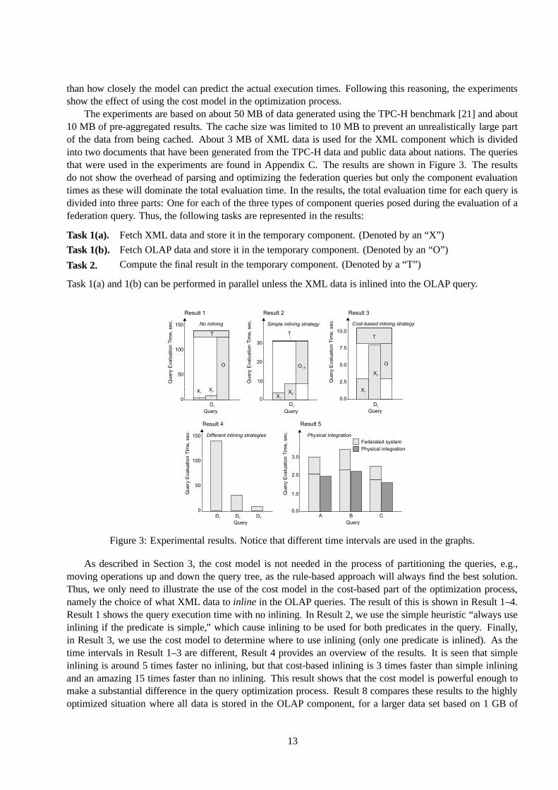
than how closely the model can predict the actual execution times. Following this reasoning, the experimentsshow the effect of using the cost model in the optimization process.

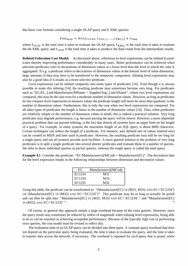
The experiments are based on about 50 MB of data generated using the TPC-H benchmark [21] and about10 MB of pre-aggregated results. The cache size was limited to 10 MB to prevent an unrealistically large partof the data from being cached. About 3 MB of XML data is used for the XML component which is dividedinto two documents that have been generated from the TPC-H data and public data about nations. The queriesthat were used in the experiments are found in Appendix C. The results are shown in Figure 3. The resultsdo not show the overhead of parsing and optimizing the federation queries but only the component evaluationtimes as these will dominate the total evaluation time. In the results, the total evaluation time for each query isdivided into three parts: One for each of the three types of component queries posed during the evaluation of afederation query. Thus, the following tasks are represented in the results:

Task 1(a). Fetch XML data and store it in the temporary component. (Denoted by an “X”)

Task 1(b). Fetch OLAP data and store it in the temporary component. (Denoted by an “O”)

Task 2. Compute the final result in the temporary component. (Denoted by a “T”)

Task 1(a) and 1(b) can be performed in parallel unless the XML data is inlined into the OLAP query.

Query

Different inlining strategies

Qu

ery

Eva

lua

tio

n T

ime

, se

c.

D2 D3D1

0

50

150

100

Physical integration

Qu

ery

Eva

lua

tio

n T

ime

, se

c.

A C

Query

B0.0

1.0

3.0

Query

Cost-based inlining strategy

Qu

ery

Eva

lua

tio

n T

ime

, se

c.

D3

T

X1

X2

O

0.0

2.5

7.5

10.0

5.0

2.0

Query

No inlining

Qu

ery

Eva

lua

tio

n T

ime

, se

c.

D1

T

X1X2

O

0

50

150

100

Query

Simple inlining strategy

Qu

ery

Eva

lua

tio

n T

ime

, se

c.

T

D2

X1

X2

O1-6

0

10

30

20

Federated system

Physical integration

Result 1

Result 4

Result 2

Result 5

Result 3

Figure 3: Experimental results. Notice that different time intervals are used in the graphs.

As described in Section 3, the cost model is not needed in the process of partitioning the queries, e.g.,moving operations up and down the query tree, as the rule-based approach will always find the best solution.Thus, we only need to illustrate the use of the cost model in the cost-based part of the optimization process,namely the choice of what XML data to inline in the OLAP queries. The result of this is shown in Result 1–4.Result 1 shows the query execution time with no inlining. In Result 2, we use the simple heuristic “always useinlining if the predicate is simple,” which cause inlining to be used for both predicates in the query. Finally,in Result 3, we use the cost model to determine where to use inlining (only one predicate is inlined). As thetime intervals in Result 1–3 are different, Result 4 provides an overview of the results. It is seen that simpleinlining is around 5 times faster no inlining, but that cost-based inlining is 3 times faster than simple inliningand an amazing 15 times faster than no inlining. This result shows that the cost model is powerful enough tomake a substantial difference in the query optimization process. Result 8 compares these results to the highlyoptimized situation where all data is stored in the OLAP component, for a larger data set based on 1 GB of

13

TPC-H data, showing three different uses of XML data, namely in a decoration query (A), in a grouping query(B), and in a selection query (C). We see that the federated OLAP-XML approach is only 30% slower than theintegrated OLAP approach (which is very inflexible w.r.t. changing data), a surprising result that is largely dueto the effectiveness of the query optimization process and the cost model.

9 Conclusion

The ever-changing data requirements of today’s dynamic businesses are not handled well by OLAP systems.Physical integration of new data into OLAP systems is a long and time-consuming process, making logicalintegration, or federation, the better choice in many cases. The increasing use of XML, e.g., in B2B applica-tions, suggests that the required data will often be available in XML format. Thus, federations of OLAP andXML databases will be very attractive in many situations. This creates a need for an efficient implementationof OLAP-XML federations which requires cost-based optimization, and, in turn, an effective cost model forOLAP-XML federations.

Motivated by this need we have presented a cost model for OLAP-XML federations. Also, techniquesfor estimating cost model parameters in an OLAP-XML federation were presented. The paper also presentedthe cost models for the autonomous OLAP and XML components on which the federation cost model wasbased. The cost model was used as the basis for effective cost-based query optimization process in OLAP-XML federations. Experiments showed that the cost model is powerful enough to make a substantial differencein for the query optimization.

We believe this paper to be the first to propose a cost model for OLAP-XML federation queries, along withtechniques for estimating and maintaining the necessary statistics for the cost models. Also, we believe theproposed cost models for the autonomous OLAP and XML components to be novel.

Future work will focus on how to provide better cost estimates when querying autonomous OLAP com-ponents and, in particular, autonomous XML components. For this purpose, extensive testing of commercialOLAP and XML database systems is needed. Also, better ways of obtaining cost parameters from the OLAPand XML components can probably be derived by an extensive examination of commercial systems.

References[1] J. A. Blakeley, W. J. McKenna, and G. Graefe. Experiences building the open oodb query optimizer. In Proceedings

of the SIGMOD Conference, pp. 287–296, 1993.

[2] S. Chawathe, H. Garcia-Molina, J. Hammer, K. Ireland, Y. Papakonstantinou, J. D. Ullman, and J. Widom. TheTSIMMIS project: Integration of heterogeneous information sources. In Proceedings of the 16th Meeting of theInformation Processing Society of Japan, pp. 7–18, 1994.

[3] W. Du, R. Krishnamurthy, and M.-C. Shan. Query Optimization in a Heterogeneous DBMS. In Proceedings of the18th VLDB Conference, pp. 277–291, 1992.

[4] R. Elmasri and S. B. Navathe. Fundamentals of Database Systems. Addison-Wesley, third edition, 2000.

[5] G. Gardarin, F. Sha, and Z.-H. Tang. Calibrating the Query Optimizer Cost Model of IRO-DB, an Object-OrientedFederated Database System. In Proceedings of the 22nd VLDB Conference, pp. 378–389, 1996.

[6] G. Graefe, R. Bunker, and S. Cooper. Hash Joins and Hash Teams in Microsoft Sql Server. In Proceedings of 24thVLDB Conference, pp. 86–97, 1998.

[7] J. M. Hellerstein, M. Stonebraker, and R. Caccia. Independent, Open Enterprise Data Integration. IEEE DataEngineering Bulletin, 22(1):43–49, 1999.

[8] H. Lu, K.-L. Tan, and S. Dao. The Fittest Survives: An Adaptive Approach to Query Optimization. In Proceedingsof 21st VLDB Conference, pp. 251–262, 1995.

[9] J. McHugh and J. Widom. Query Optimization For XML. In Proceedings of 25th VLDB Conference, pp. 315–326,1999.

[10] H. Naacke, G. Gardarin, A. Tomasic. Leveraging Mediator Cost Models with Heterogeneous Data Sources. InProceedings of the 14th ICDE Conference, pp. 351–360, 1998.

14

[11] C. Ozkan, A. Dogac, and M. Altinel. A Cost Model for Path Expressions in Object-Oriented Queries. Journal ofDatabase Management 7(3), 1996.

[12] D. Pedersen, K. Riis, and T. B. Pedersen. A Powerful and SQL-Compatible Data Model and Query Language forOLAP. To appear in Proceedings of the 13th ADC Conference, 10 pages, 2002.

[13] D. Pedersen, K. Riis, and T. B. Pedersen. XML-Extended OLAP Querying. Submitted for publication, 2002.

[14] D. Pedersen, K. Riis, and T. B. Pedersen. Query Processing and Optimization for OLAP-XML Federations. Sub-mitted for publication, 2002.

[15] T. B. Pedersen, A. Shoshani, J. Gu, and C. S. Jensen. Extending OLAP Querying To External Object Databases. InProceedings of the 9th CIKM Conference, pp. 405–413, 2000.

[16] M. T. Roth, F. Ozcan, and L. M. Haas. Cost models do matter: Providing cost information for diverse data sourcesin a federated system. In Proceedings of 25th VLDB Conference, pp. 599–610, 1999.

[17] A. P. Sheth and J. A. Larson. Federated Database Systems for Managing Distributed, Heterogeneous, and Au-tonomous Databases. ACM Computing Surveys, 22(3):183–236, 1990.

[18] A. Shukla, P. Deshpande, J. F. Naughton, and K. Ramasamy. Storage Estimation for Multidimensional Aggregatesin the Presence of Hierarchies. In Proceedings of 22nd VLDB Conference, pp. 522–531, 1996.

[19] Software AG. Tamino XML Database. http://www.softwareag.com/taminoplatform, 2001. Currentas of January 15, 2001.

[20] E. Thomsen. OLAP Solutions: Building Multidimensional Information Systems. Wiley, 1997.

[21] Transaction Processing Council. TPC-H. http://www.tpc.org/tpch, 2001. Current as of January 15, 2001.

[22] W3C. Extensible Markup Language (XML) 1.0 (Second Edition). http://www.w3.org/TR/REC-xml, Oc-tober 2000. Current as of January 15, 2001.

[23] W3C. Xml schema part 0: Primer. http://www.w3.org/TR/xmlschema-0, May 2001. Current as ofJanuary 15, 2001.

[24] Q. Zhu and P.-Å. Larson. Global Query Processing and Optimization in the CORDS Multidatabase System. InProceedings of the 9th PDCS Conference, pp. 640–646, 1996.

[25] Q. Zhu and P.-Å. Larson. Developing Regression Cost Models for Multidatabase Systems. In Proceedings of the4th PDIS Conference, pp. 220–231, 1996.

[26] Q. Zhu, Y. Sun, and S. Motheramgari. Developing Cost Models with Qualitative Variables for Dynamic Multi-database Environments. In Proceedings of the 16th ICDE Conference, pp. 413–424, 2000.

A Details of the OLAP Component Cost Model

This section provides detail on the estimation and maintenance of the OLAP cost parameters.

Estimating OLAP Cost Parameters: The cost parameters %5&)(+*�,N0O&)P , % &)(+*�,N0 Q_R ��T , and %4&)(+*�,^0U:�V � E � are esti-mated as follows. The first parameter %A&)(+*�,N0O&)P is assumed to be constant, and is estimated by timing a probingquery posed to the OLAP component. The probing query specifies a single measure and one particular combi-nation of dimension values all belonging to bottom levels of the cube. Assuming that the cube has indexes ondimension values, the evaluation time of such a query is negligible. Also, the query returns at most one value,which means that little or no time is used on transporting data from the OLAP component. Hence, %·&)(+*�,N0O&)Pincludes the full processing and network communication time of a query except the time it takes to actuallyproduce the result and to transfer the result over the network. A better estimate can be achieved by using theaverage time for a number of queries.

The estimate of %�&)(+*�,N0U:V � E � for a query � is calculated from the estimated result size and the network datatransfer rate: %4&)(+*�,^0U:�V � E �." �r�U� u $|�à$|� 7�7tvu ��wW�+xmyzv{A�|{'}~{A� u $|� 7Both

�r�O� u $|�à$|� 7�7 andt�u ��wW�+xmyzv{A�|{'}�{�� u $|� 7 are estimated as described above. However, if the OLAP com-

ponent is also used as temporary component, % &)(+*�,N0U:V � E � is set to zero cost.

15

The evaluation cost % &)(+*�,N0 QSR ��T can be estimated in two ways. The simplest is to use the formula forø ¶ Ü ¸�ù @|ú µdirectly and base all evaluation cost estimates on a single estimate of the cube size. Alternatively,

the estimated cost for a query can be based on the measured cost for a similar query that has been posed earlier.The cost can be measured from a probing query or a user query. A list of these queries can be maintainedtogether with their measured cost and used to compute the cost of future queries. The latter should intuitivelyprovide the best estimates, since it is based on an actual measured cost for a similar query. This approach isdescribed in more detail in the following.

Using the second method, % &)(+*�,N0 Q_R ��T is estimated from a set of probing queries and the statistical infor-mation presented above. The probing queries are used to estimate the query evaluation time and result size ofqueries that aggregates the cube to a certain combination of levels without performing any selections. From thisestimate the size and evaluation time of a given query can be calculated using the functions presented above.Queries that retrieve all data at a given combination of levels cannot generally be posed directly, and insteadthe size and evaluation time of such a query � * T®T is estimated by posing a probing query � ,_V�H ��� as describedlater. These estimated results are stored for each cube � in a table containing a row for each query � * TMT :

Columns Descriptionz������ -333'- z���� E The combination of levels to which the cube is rolled up in � f nMn�r�U� u $��Ë$ � 7�7 The estimated size of the result of � f nMn� �+{ �|� ��� u�� ? ¥���� q��<l�� � The estimated evaluation time of � f nMn when preaggr. may have been used� �+{ �|� ��� u � ? ¥��"!$#�¥�� q���l � � The estimated evaluation time of � f nMn when preaggr. have not been used� � u x��_�����·�r�

The number of user queries that has rolled up to the same levels as � f nMn% x u z������ -3334- % x u z���� E The level of pre-aggregation that is assumed to be used to evaluate � f nMnTable 2: The Statistics Stored for OLAP Queries

Due to the typically large amounts of data stored in OLAP databases, it is often unfeasible to fetch theentire cube to get the size estimate and evaluation time estimates. This is especially true for the lower levelaggregates, whereas the amount of data at higher aggregation levels can often be retrieved in its entirety. Instead,probing queries are used that select a certain percentage of the facts on the specified levels, that is, selectionsare performed on dimension values to keep the size of the returned result reasonable. Notice that if the simplesize based method is used, it is sufficient to use probing queries like “SELECT COUNT(*) FROM F” to estimatethe size. However, when using the second method the time must also be measured.

Example A.1 Here is an example of a query that can be expected to select approximately 25% of the cubedata, because all bottom values are selected in the ECs dimension, while 50% are selected in both the Suppliersand Time dimensions:

SELECT SUM (Cost), SUM (NoOfUnits), Class(EC), Country(Supplier), Year(Day)FROM PurchasesWHERE Class IN (’FF’, ’L’) AND Country IN (’US’) AND Year(Day) IN (’2000’)GROUP BY Class(EC), Country(Supplier), Year(Day)

Assuming a uniform distribution of facts in the cube this returns around 25% of the data. In a real examplesmaller amounts of data are used. BEach probing query is timed resulting in %m�N���! K¡O¢ , and the size of the result is measured, resulting in

�r�U� u �N���! K¡O¢ .Again, assuming that facts are distributed uniformly in the cube, the actual size of the cube without the se-lections

�r�O� u � ª'& & can then be estimated based on�r�U� u � ���! K¡O¢ by using the

�r�O� ufunction mentioned in Ta-

ble 1. Likewise, the evaluation time� ��{ �K� ��� u � ª(& & can be estimated using the approximation %��N���! K¡O¢ "

%�d9e)f�g 0O&)P 8 � �+{ �|� ��� u � ���! K¡O¢ 8 Ó �2Ô � ¦ ���� K¡�¢G � F*)hHIV�+-, � F �$._� F � ��£9¤ and the definition of ø ¶ Ü ¸�ù @`ú µ. Two different values of

the evaluation time are needed to provide good estimates for both queries that may make use of pre-aggregation

16

and for queries that cannot use pre-aggregation, because some selection refers to unaggregated measures. Tomeasure these values two probing queries are used: One that performs selection only on dimension valuesas described above, and one that also contains a selection on a measure in the WHERE clause. This forcesthe OLAP component to access the base cube directly, in effect disabling the use of pre-aggregated results.The problem with using the definition of ø ¶ Ü ¸�ù @|ú µ

is that it is not generally possible to know which pre-aggregations are used. Hence, an adaptive strategy is used as discussed in the presentation of ø ¶ Ü ¸�ù @|ú µabove. However, if

� ��{ �|� ��� u � ? ¥���� q���l � �0/ � ��{ �|� ��� u � ? ¥��"!$#�¥(� q/��l ��� , we can conclude that no pre-aggregationshave been used even though the probing query permitted it. To support this adaptive strategy, the columns% x u z������ -333'- % x u zÃ��� E contains the current guess at which level of pre-aggregation is used.

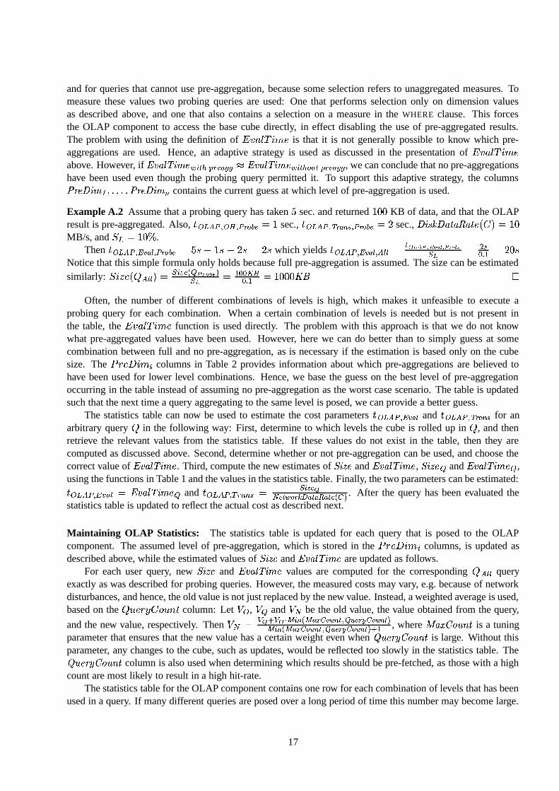
Example A.2 Assume that a probing query has taken 1 sec. and returned  232 KB of data, and that the OLAPresult is pre-aggregated. Also, % &)(+*�,N0O&)P�0 ,SV�H ��� "  sec., % &)(+*�,N0U:V � E � 0 ,_V�H ��� " è sec.,

zÃ���oy�zv{A�|{'}�{A� u $|� 7 "  2MB/s, and í e "  254 .

Then % &)(+*�,N0 Q_R �IT 0 ,SV�H ��� " 1 � ¿  � ¿ è � " è � which yields % &)(+*�,N0 Q_R �IT 0 * TMT " ¥ ¨�©oª �5« 6�7�¯ & « ���! K¡O¢�(8 " c s9;: 1 " è 2 �Notice that this simple formula only holds because full pre-aggregation is assumed. The size can be estimatedsimilarly: íÉ@`õ µ $|� f nMn�7 " � ?O�I�o���=<5>�?A@CB<¤�'8 " 1 9D9�E �9;: 1 "  232325FHG B

Often, the number of different combinations of levels is high, which makes it unfeasible to execute aprobing query for each combination. When a certain combination of levels is needed but is not present inthe table, the ø ¶ Ü ¸�ù @`ú µ

function is used directly. The problem with this approach is that we do not knowwhat pre-aggregated values have been used. However, here we can do better than to simply guess at somecombination between full and no pre-aggregation, as is necessary if the estimation is based only on the cubesize. The Iؾ µ ó @|ú ? columns in Table 2 provides information about which pre-aggregations are believed tohave been used for lower level combinations. Hence, we base the guess on the best level of pre-aggregationoccurring in the table instead of assuming no pre-aggregation as the worst case scenario. The table is updatedsuch that the next time a query aggregating to the same level is posed, we can provide a better guess.

The statistics table can now be used to estimate the cost parameters % &)(+*�,N0 QSR ��T and %4&)(+*�,N0U:V � E � for anarbitrary query � in the following way: First, determine to which levels the cube is rolled up in � , and thenretrieve the relevant values from the statistics table. If these values do not exist in the table, then they arecomputed as discussed above. Second, determine whether or not pre-aggregation can be used, and choose thecorrect value of

� ��{ �|� ��� u. Third, compute the new estimates of

�r�O� uand

� ��{ �|� ��� u,�r�U� u � and

� �+{ �K� ��� u � ,using the functions in Table 1 and the values in the statistics table. Finally, the two parameters can be estimated:% d9e)f�g 0 j9kolmn " � �+{ �|� ��� u � and % d9e)f�g 0 prq�l ZAs " Ó �2Ô � ¦G � F*))H�V�+-, � F �$._� F � ��£9¤ . After the query has been evaluated thestatistics table is updated to reflect the actual cost as described next.

Maintaining OLAP Statistics: The statistics table is updated for each query that is posed to the OLAPcomponent. The assumed level of pre-aggregation, which is stored in the Iؾ µ ó @|úÀ? columns, is updated asdescribed above, while the estimated values of

���O� uand

� ��{ �|� ��� uare updated as follows.

For each user query, new�r�U� u

and� ��{ �|� ��� u

values are computed for the corresponding � * TMT queryexactly as was described for probing queries. However, the measured costs may vary, e.g. because of networkdisturbances, and hence, the old value is not just replaced by the new value. Instead, a weighted average is used,based on the �KJ µ ¾+ñ_� × JrC9% column: Let L d , Lr� and LNM be the old value, the value obtained from the query,

and the new value, respectively. Then LOM "QP ¦ � P"R=S � � EA�O� �-T � H � EF|0VU ��� V�W � H � EF�¤� � EA�O� �-T � H � EF|0VU ��� V�W � H � EF�¤C�]1 , where X { � �����·�r� is a tuningparameter that ensures that the new value has a certain weight even when � � u xm�_�����·�r�

is large. Without thisparameter, any changes to the cube, such as updates, would be reflected too slowly in the statistics table. The� � u xm�_�����·�r�

column is also used when determining which results should be pre-fetched, as those with a highcount are most likely to result in a high hit-rate.

The statistics table for the OLAP component contains one row for each combination of levels that has beenused in a query. If many different queries are posed over a long period of time this number may become large.

17

In that case, the size can be kept at a fixed level by expiring old and less frequently used combinations eachtime a new row is added.

B Details of the XML Component Cost Model

This section provides detail on the estimation and maintenance of the OLAP cost parameters.

The choice of which probing queries can be used depends on the type of the link. Three different types ofprobing queries are used as shown here:

No. Query Measured values

Probe1 / Y [false()] timeProbe2 /E Z [position()=i Z [ / \�\]\ /E ^ [position()=i _ ] fanout, cardinalityProbe3 /base[locator= `�a ] (Natural links) time, size, fanout,

/locator b$c (Enumerated links) cardinality, min value,for C random values of @ max value

From Probe1 the query overhead % ��>(�0O&)P can be estimated. The assumptions are that no data is returnedand that the work performed by this query will always have to be performed. Hence, it represents the minimumtime it takes to perform a query. This may include everything from parsing the entire XML document to parsingonly the query. In either case it is a reasonable approximation to the constant overhead, which will often bedominated by the server response time. However, sometimes a clever parser may discover that this query alwaysproduces an empty result and avoid most of the query overhead. In that situation, requesting a leaf node wouldusually provide a better estimate of the overhead. By running the probing query a number of times a moreprecise average value can be found.

A number of queries on the form of Probe2 are used to find the fanout and cardinality of the elementsabove and including the nodes pointed to by the link. For smaller amounts of XML data, this is done by simplyretrieving all the nodes. However, for large amounts of data this may not be feasible, and another method mustbe used. Since XPath does not allow computed values such as count() to be returned, binary search is used tofind the maximum value @ ð of position() for which any data is returned. The idea is to find the number of valueson the first level, use a sample of these to estimate the number of values on the second level, use a sample ofthese to estimate the number of values on the third level, and so on. Most of these queries will work on data thathas already been retrieved, and hence, only a few queries will actually retrieve data. However, these queriesmay return large amounts of data because they refer to nodes close to the root node. If this is not feasible, aguess is made at the number of nodes.

Probe3 is used to find statistical information about the nodes below the nodes pointed to by the link. Asample of the nodes pointed to is retrieved using Probe3 for the given type of link. The nodes are then analyzedlocally to find the remaining information:

� {A�����S�,��{+x�ÿ+����{ � �����

and���O� u

of the remaining elements, as wellas maximum and minimum values for numerical nodes. The time and size of the queries are measured andused in the computation of

zv{A�|{'}~{A� u. Where several links exist for a single document, only one set of probing

queries is performed. All the statistical information obtained from the probing queries is stored in the federationmetadata for each XML document.

The combination of a limited interface and almost no knowledge about the underlying source can some-times make the probing of XML components expensive. Several optimizations are possible, including theretrieval of larger parts of the document in a single query [14]. However, probing may still be a problem forvery slow XML components, e.g. on the Web. Hence, the default behavior is not to perform probing immedi-ately, when a link is created, but instead wait until the system load has been low for a while. When no probinghas been performed, nothing is known about the component, and instead a predefined set of cost values areused. The probing can also be disabled for very slow components.

18

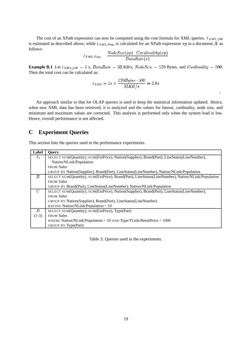
The cost of an XPath expression can now be computed using the cost formula for XML queries. %' ��>(�0O&)Pis estimated as described above, while %� ��#(�0 ,SV�H is calculated for an XPath expression � Ú in a document d asfollows: % ��#(A0 ,_V�H " t ��ÿ u �r�O� u $�� Ú 7 X+�ØÜh¾+½5@|C^Ü ¸ @`%<ñ9$�� Ú 7zv{A�|{'}�{�� u $�� 7Example B.1 Let %I ��#(50O&)P "  s,

zv{A�|{'}�{�� u " ê è KB/s,t ��ÿ u �r�U� u "  è 2 Bytes, and

��{Ax/ÿ+����{ � ����� " 1�232 .Then the total cost can be calculated as:

%/ ��#( "  � 8  è 25G �A� u � X�1�232ê è FHGvþ � / è 3fe �B

An approach similar to that for OLAP queries is used to keep the statistical information updated. Hence,when new XML data has been retrieved, it is analyzed and the values for fanout, cardinality, node size, andminimum and maximum values are corrected. This analysis is performed only when the system load is low.Hence, overall performance is not affected.

C Experiment Queries

This section lists the queries used in the performance experiments.

Label Queryg Z SELECT SUM(Quantity), SUM(ExtPrice), Nation(Supplier), Brand(Part), LineStatus(LineNumber),Nation/NLink/Population

FROM SalesGROUP BY Nation(Supplier), Brand(Part), LineStatus(LineNumber), Nation/NLink/PopulationhSELECT SUM(Quantity), SUM(ExtPrice), Brand(Part), LineStatus(LineNumber), Nation/NLink/PopulationFROM SalesGROUP BY Brand(Part), LineStatus(LineNumber), Nation/NLink/PopulationiSELECT SUM(Quantity), SUM(ExtPrice), Nation(Supplier), Brand(Part), LineStatus(LineNumber),FROM SalesGROUP BY Nation(Supplier), Brand(Part), LineStatus(LineNumber)HAVING Nation/NLink/Population > 10jSELECT SUM(Quantity), SUM(ExtPrice), Type(Part)

(1-3) FROM SalesWHERE Nation/NLink/Population > 10 AND Type/TLink/RetailPrice < 1000GROUP BY Type(Part)

Table 3: Queries used in the experiments.

19