Embed Size (px)
Citation preview

Microscopie électronique et traitement d’images
Cours N°2 Traitement d’images Structure d’objets biologiques
dans les 3D
Master informatique spécialité IMA
Prof. Catherine Vénien-Bryan!
Institut de minéralogie et de physique des milieux condensés (IMPMC)!
CNRS UMR 7590, UPMC!
E-mail: [email protected]!
Traitement d’images
Particules isolées, protéines macromolécules, petits
virus (haute résolution) •" Numérisation de l’image, cameras CCD
•" Sélection des particules et normalisation du contraste
•" Analyse dans les 2dimensions:
•" Alignement
•" Classification des images
•" Création du modèle dans les 3 dimensions et raffinement
•" Méthode des séries coniques aléatoires
•" Lignes communes (transformée de Radon)
•" Raffinement
Cellules entières, bactéries virus (moyenne résolution) •" Tomographie électronique cellulaire

Digital images Sampling and grey level
Discrétisation spatiale et quantification
Image Digitization
Original image Image sampled
at low resolution
Grey level resolution:
one bit can code for 2 states: “0” or “1”
Byte (octet): a string of 8 bits
can code for 28 = 256
different states
Pixel size
The image must be divided up into
pixels (sampled) at a spacing at least twice as fine as the finest
detail (highest frequency) to be analysed.
(in practice, 3-4x as fine).
Each picture element
stored in the computer, with its own grey level, is
called a pixel.
Digital images Sampling-1
!"#$%&'%($)$#***%

Digital images Sampling -3 - spatial resolution
Théorème de Nyquist-Shannon
Nyquist-Shannon frequency: the
sampling frequency is twice the highest frequency term being
represented.
If the same sampling frequency is
used for a higher frequency wave, the sample points do not follow the
oscillations. The features will not be correctly represented in the image.
Remember that the image can be represented as the sum
of a series of sinusoidal waves. The highest frequency wave term present defines the resolution limit. When an
image is digitised, the wave components are sampled at an interval defined by the scanner step size.
•" In practice, it is necessary to sample at 3-4x the
resolution, to avoid numerical rounding errors.
Digital images Scanning – number of grey levels-1
144 72 16
8 4 2

Noise reduction by averaging
Averages of 2 5 10 25 200 images
Raw
images
Variance
For a stack of aligned images, the
variance can be calculated for each
pixel, to give a map of variations
between the images in the data set.
This can help to assess the reliability
of features seen on the average
image, and can reveal if images of
different structures are mixed up in
the same data set.
The variance is determined for each pixel as the difference
between the pixel value in a given image and the average
value of that pixel in all the images. This difference is squared
and the sum of these squares is calculated for all the images in
the stack.
Variance = [1/(N-1)] ![Pi(rj) - Pav (rj)]2
where Pi(rj) is the value of pixel j in image i and Pav (rj) is the
average value of pixel j in all the images, for a set of N images.
i,,j

!"#$%&'()*+,#-'&()#"&($'&(./(
01$'234"()'&(5#6327$'&(8+$,"-./0&0%!"#$%&'()*+*9(
Normalisation du contraste
Soustraction de la moyenne et division par l’écart type

Alignement et fonctions de corrélation
Corrélation croisée 2D
1%2%3$4% 5%2%6,/7$%
and =
5%$'8%8#/0'9/8:%$8%;%-+/<=$%>"'&?"0%@$%5%%
$0%A%$8%B%=0%0"=C$/=%-"$D-&$08%@$%-"##:9/?"0%%
$'8%-/9-=9:E%
F$%#:'=98/8%G0/9%$'8%=0$%-/#8$%(&@&,$0'&"00$99$%@"08%9/%8/&99$%%
-"##$'>"0@%;%-$99$%@$'%&,/7$'%@H"#&7&0$%$8%<=&%>"''I@$%=0%%
>&-%@$%-"##:9/?"0%<=&%-"##$'>"0@%;%9/%8#/0'9/?"0%@$%5%>"=#%%
9/<=$99$%9$'%@$=J%@&'<=$'%'$%'=>$#>"'$08%>/#4/&8$,$08E%
F/%>"'&?"0%@=%>&-%>/#%#/>>"#8%;%9H"#&7&0$%K-$08#$%@$%9/%-/#8$L%
-"##$'>"0@%/=%C$-8$=#%@$%8#/0'9/?"0%;%/>>9&<=$#%>"=#%
#$-$08#$#%9H&,/7$%5%>/#%#/>>"#8%;%9H&,/7$%1%KJ%MNO%P%.%QNOLE%%
.%
A%
RR%%SK&PTL%E%4K&M0PTM,L%
SK&PTL% 4K&PTL%
A%8#/0'9/?"0%0%2%U%%
B%8#/0'9/?"0%,%2%U%
Alignement et fonctions de corrélation
Fonction d’Auto-Corrélation = FAC
VH$'8%9/%-"##:9/?"0%-#"&':$%@H=0$%&,/7$%/C$-%$99$Q,W,$%
6,/7$% 1VX%

Corrélation croisée angulaire
Y0$%&,/7$%5%K'=>>"':$%-$08#:$L%$'8%>9/-:$%'=#%=0$%%
&,/7$%@$%#:4:#$0-$P%$8%>"=#%-+/<=$%#"8/?"0%@$%5P%"0%,$'=#$%
9$=#%-"$D-&$08%@$%-"##:9/?"0E%
Alignement et fonctions de corrélation
#$4%
5%
3"8/?"0%/079$%
-"##$9/?"0%
F/%-"##:9/?"0%$'8%-/9-=9:$%'=#%=0$%':#&$%@$%%
#/."0'%$8%9/%C/9$=#%79"(/9$%$'8%&0'-#&8$%$0%%
4"0-?"0%@$%9H/079$%@$%#"8/?"0E%
Exemple d’alignement sur une référence
3:4:#$0-$%%%%%%%%%%%%&,/7$%5%
X1V%#$4%%%%%%%%%%%%%%%X1V%5%
V"##:9/?"0%-#"&':$%/07=9/&#$%@$'%X1V'%
!/&'%-",,$%9$'%X1V'%'"08%@$'%4"0-?"0'%>/&#$'P%
&9%.%/%=0$%/,(&7=Z8:%@$%N[U\%'=#%9H/079$%@$%
#"8/?"0%<=H"0%8#"=C$%$0%-/9-=9/08%9$=#%
-"##:9/?"0%-#"&':$%/07=9/&#$E%
]0%-/9-=9$%9$'%X1V'%@$'%&,/7$'%
>"=#%"(8$0&#%=0$%#$>#:'$08/?"0%%
-$08#:$%$8%#$^:8/08%>/#?$99$,$08%
9/%'8#=-8=#$%@$'%>/#?-=9$'E%
Alignement et fonctions de corrélation

X,/J%2%UE_N% X,/J%2%UE`a%
19&70$,$08%$8%4"0-?"0%@$%-"##:9/?"0'%
19&70$,$08%'=#%=0$%#:4:#$0-$Qb%
D’autres méthodes d’alignement ont été proposées
pour minimiser l’influence de l’image de référence.
"Reference free" iterative alignment (Penczek et al., 1992) :
1) Ici deux images sont prises au hasard, alignées et leur moyenne est alors
utilisée comme nouvelle référence pour aligner une troisième image. Le
processus se reproduit itérativement jusqu’à ce que toutes les images
soient alignées.
2) Pour minimiser l’influence de l’ordre dans lequel les images ont été choisies
pendant l’alignement, on repart ensuite à l’envers, en réalignant la première
image et en la réalignant sur (Moyenne totale - l’image 1). Puis la seconde
image est réalignée sur (Moyenne totale - l’image 2), etc …
3) Le processus entier est recommencé à nouveau sur les images issues de ce
premier cycle d’alignement (étapes 1 et 2), jusqu’à ce qu’aucune amélioration
ne soit constatée d’un cycle au suivant.
"multi-reference alignment" et d’autres méthodes d’alignement utilisent la
classification en parallèle du processus d’alignement.

:;',5$'()'(2'"<6#-'('<()*#$+-"','"<(=(>',42%#"+"?@(
:;',5$'()'(2'"<6#-'('<()*#$+-"','"<(=(>',42%#"+"?.(

A$#&&+B2#34"(./?@(
Classification 2D-2 Brétaudière JP and Frank J (1986) Reconstitution of molecule images
analyzed by correspondence analysis: A tool for structural interpretation.
J. Microsc. 144, 1-14.

A$#&&+B2#34"(./?C(
Image No1
Image No80
Pixel 1 Pixel 2754
x ij
A$#&&+B2#34"(./?D(
!/8#&-$%

Méthode de la dragée
Espace à 2754 dimensions
"b%
"c%
"N%
1J$%4/-8"#&$9%N%
1J$%4/-8"#&$9%b%
1J$%4/-8"#&$9%c%
F/%@&/7"0/9&'/?"0%@$%9/%,/8#&-$%-/##:$%T = X'X%>$#,$8%@$%@:8$#,&0$#%9/%>9='%7#/0@$%@&#$-?"0%@H$J8$0'&"0%
@$%0"'%@"00:$'% K0=/7$%@$%>"&08'L%@/0'% 9H$'>/-$%,=9?Q@&,$0'&"00$9E%V$)$%@&#$-?"0%@H$J8$0'&"0%-"##$'>"0@%;% 9/%
>9='%7#/0@$%d%C/#&/?"0%e%"=%d% 8$0@/0-$%e%/=%'$&0%@$%0"'%@"00:$'E%VH$'8% 9H/J$% 4/-8"#&$9%f\N%@"08% 9H/,>9&8=@$%$'8%
-/#/-8:#&':%>/#% 9/% C/9$=#%>#">#$%"NE%]0%$g$-8=$%/9"#'%=0%-+/07$,$08%@$% #$>I#$%>"=#%@:8$#,&0$#% 9/%>"'&?"0%@$%
-+/-=0$% @$% 0"'% @"00:$'% K&,/7$'L% >/#% #/>>"#8% ;% -$8% /J$% 4/-8"#&$9E% h=&'P% "0% #$-+$#-+$% 9/% '$-"0@$% >9='% 7#/0@$%
@&#$-?"0%@H$J8$0'&"0%d%"#8+"7"0/9$%e%;%9/%>#$,&I#$%>"=#%@:G0&#%9H/J$%4/-8"#&$9%f\b%-/#/-8:#&':%>/#%=0$%/,>9&8=@$%@$%
"bE% F$% 4/&8% <=$% 9$'% /J$'% 4/-8"#&$9'% f\N% $8% b% '"&$08% "#8+"7"0/=JP% &0@&<=$% <=H&9'% -/#/-8:#&'$08% @$'% C/#&/?"0'%
&0@:>$0@/08$'%K0"0Q-"##:9:$'LE%]0%$J>#&,$%/&0'&%>/#%"#@#$%@:-#"&''/08%8"=8$'%9$'%C/#&/0-$'%&0@:>$0@/08$'%@$%0"'%
@"00:$'%'=#%9$'%/J$'%4/-8"#&$9'%f\NP%bP%cP%i%P$8-%j%%%
A$#&&+B2#34"(./?E(A61#34"()*7"'(,#<6+2'(#(.FEG()+,'"&+4"&(

Classification 2D
a) Méthodes par partition: e.g. "Moving seeds" method
Diday E (1971) La méthode des nuées dynamiques. Rev. Stat. Appl. 19, 19-34.
Deux images prises au hasard servent de centres d’agrégation pour la partition. Les
centres de gravité de chaque classe servent de nouveaux centres d’agrégation pour un
nouveau cycle de partition. Arrêt lorsque les centres d’agrégation ne bougent plus d’un
cycle à l’autre, ou après un nombre déterminé d’itérations.

Classification 2D
b) Classification Ascendante Hiérarchique
N% b%
c%
i%
O%
N% b%
c%
i%
O%N% c%
a%
a%
O%b%
`%
`%
i%
[%
[%

H'I'6'"2'&(
k+/&S+%lEP%m/"P%nEP%5/J8$#PoElEP%1'8=#&/'P%XEpEP%5"&''$8P%fEP%F$&8+P%1EP%/0@%X#/0SP%pE%KbUU[L%kh6qr3%&,/7$%>#"-$''&07%
4"#%'&079$Q>/#?-9$%#$-"0'8#=-?"0%"4%(&"9"7&-/9%,/-#","9$-=9$'%4#",%$9$-8#"0%,&-#"7#/>+'%,*-./"&
0/(-(1(#2&c%KNbL%N_iNQN_`iE%
V/##/7+$#%5P%s&''$($#8+%fP%s#&$7,/0%qP%!&99&7/0%31P%h")$#%VkP%h=9"S/'%pP%3$&9$&0%1%KbUUUL%F$7&0"0t%/0%
/=8",/8$@%'.'8$,%4"#%/-<=&'&?"0%"4%&,/7$'%4#",%C&8#$"='%&-$%'>$-&,$0'E%34&5-/.1-4&6$(#(78%NcbP%ccQiOE%%
h")$#%VkP%V+=%nP%X#$.%5P%m#$$0%VP%s&''$($#8+%fP%!/@@$0%lpP%!&99$#%sFP%f/+#'8$@8%sP%h=9"S/'%pP%3$&9$&0%1P%l-+$07%
qP%o$($#%qP%V/##/7+$#%5E%KN___L%X#/0SP%pE%KN_`OLE%1C$#/7&07%"4%9"u%$J>"'=#$%$9$-8#"0%,&-#"7#/>+'%"4%
0"0>$#&"@&-%"(T$-8'4&9#-/*)$1/(21('8%NP%NO_QNabE%
X#/0SP%pEP%/0@%19Q19&P%FE%KN_`OLE%k&70/9Q8"Q0"&'$%#/?"%"4%$9$-8#"0%,&-#"7#/>+'%"(8/&0$@%(.%-#"''Q-"##$9/?"0E%
,*-./"%bOaP%c`aQc`[E%
X#/0S%pE%KN__aL%l+#$$Q@&,$0'&"0/9%,&-#"'-">.%"4%,/-#","9$-=9/#%/''$,(9&$'E%:1*;")$1&0/"22P%k/0%q&$7"E%
X#/0S%pE%KN__UL%V9/''&G-/?"0%"4%,/-#","9$-=9/#%/''$,(9&$'%'8=@&$@%/'%v'&079$%>/#?-9$'vE%w=/#8E%3$CE%5&">+.'E%bcP%
b[NQcb_E%
n$0@$#'"0P%3EP%/0@%m9/$'$#P%3E!E%KN_[OLE%w=/0?8/?C$%/0/9.'&'%"4%&,/7$%-"08#/'8%&0%$9$-8#"0%,&-#"7#/>+'%"4%
($/,Q'$0'&?C$%-#.'8/9'E%9#-/*)$1/(21('8%NaP%Nc_QNOUE%
n$0@$#'"0P%3E%KN__OLE%l+$%>"8$0?/9%/0@%9&,&8/?"0'%"4%0$=8#"0'P%$9$-8#"0'%/0@%AQ#/.'%4"#%/8",&-%#$'"9=?"0%
,&-#"'-">.%"4%=0'8/&0$@%(&"9"7&-/9%,"9$-=9$'E%w=/#8E%3$CE%5&">+.'E%b[P%N`NQN_cE%
k/J8"0P%oE]E%KN__iL%1--=#/8$%/9&70,$08%"4%'$8'%"4%&,/7$'%4"#%'=>$#Q#$'"9C&07%/>>9&-/?"0'P%34&<$1/(21E%N`iP%
aNQa[E%
C/0%n$$9P%!E%KN_[_LE%V9/''&G-/?"0%"4%C$#.%9/#7$%$9$-8#"0%,&-#"'-">&-/9%&,/7$%@/8/%'$8'E%='+>%G.P%NNiQNba%%
k:#&$%@$%>#"T$-?"0'%
&0-9&0:$'%
V/9-=9%@H=0%C"9=,$%
@$%#$-"0'8#=-?"0%cq%%
>/#%#:8#">#"T$-?"0%
J6+"2+5'()'($#(<4,4-6#5>+'(,4$127$#+6'(8@9%%

2%5
4 3
6
7 1
r'>/-$%@$%X"=#&$#%
1 2 7 6 5 4 3
l+:"#I,$%@$%9/%'$-?"0%-$08#/9$t%
r0%$'>/-$% #:-&>#"<=$P% 8"=8$%>#"T$-?"0%(&Q
@&,$0'&"00$99$% @H=0% "(T$8% -"##$'>"0@% ;%
=0$% '$-?"0% -$08#/9$% @/0'% 9/% 8#/0'4"#,:$%
@$% X"=#&$#% cq% @$% 9H"(T$8E% V+/<=$% '$-?"0%
-$08#/9$% $'8% "#&$08:$% >$#>$0@&-=9/&#$,$08%
;% 9/% @&#$-?"0% @$% >#"T$-?"0% K@&#$-?"0% @=%
4/&'-$/=%@H:9$-8#"0'LE%%
J6+"2+5'()'($#(<4,4-6#5>+'(
8&16+'&(+"2$+"1'&9(8.9%%
X
y
Z
# $ % %
X
Y
Z
F$'%-"0C$0?"0'%kh6qr3%
-"0-$#0/08%9$'%/079$'%$=9:#&$0'E%
#" = phi = rotation autour de Z&$ = theta = rotation autour de Y&% = psi = rotation autour de Z

A4"<6#+"<'()'($#(26%4K:L(&76(4MN'<&(M+4$4-+O7'&(P(
l#/C/&99$#%;%4/&(9$%@"'$%@v:9$-8#"0'%KNU$QxybL%
k$=9$,$08%N%K"=%bL%>#&'$K'L%@$%C=$K'L%%>/#%z"0$%
V"99$-8$#%f%&,/7$'%;%4/&(9$%#/>>"#8%'&70/9x(#=&8%
1C$-%=0$%4"#8$%'"='Q4"-/9&'/?"0%K-"08#/'8$L%
V/9-=9$#%@$'%,".$00$'%0=,:#&<=$'%bq%"=%cq%
V"##&7$#%9/%4"0-?"0%@$%8#/0'4$#8%@$%-"08#/'8$%KVlXL%
Y?9&'$#%9$'%'.,:8#&$'%$8x"=%@&'>"'&?"0%@$'%>/#?-=9$'t%
k.,:8#&$%+:9&-"Z@/9$P%&-"'/:@#/9$P%#:'$/=J%bqP%
"=%>/'%@$%'.,:8#&$E%
Q#(6'24"&<67234"()*7"(,4)R$'(561$+,+"#+6'(C/(
L’acquisition des séries coniques aléatoires
Les méthodes de reconstructions
0°
45°
1%
2%
5
4 3
6 7 8 1 2 8 7 6 5 4 3
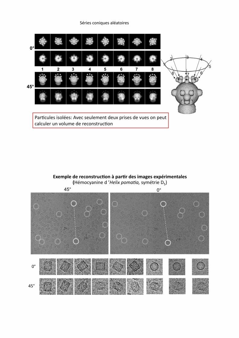
h/#?-=9$'%&'"9:$'t%1C$-%'$=9$,$08%@$=J%>#&'$'%@$%C=$'%"0%>$=8%%
-/9-=9$#%=0%C"9=,$%@$%#$-"0'8#=-?"0%
k:#&$'%-"0&<=$'%/9:/8"&#$'%
U\%
iO\%
45°% 0°
U\%
iO\%
:;',5$'()'(6'24"&<67234"(S(5#636()'&(+,#-'&(';516+,'"<#$'&%8n:,"-./0&0$%@%H!"#$%&'()*+*?&'.,:8#&$%qOL%

{=$'%@$%-|8:%(#=8$'% !W,$'%&,/7$'%/9&70:$'%
19&70$,$08%
q:8$#,&0/?"0%
@$%9%H/079$%K')&
V9/''&G-/?"0%/=8",/?<=$%!%O%C=$'%
V/9-=9%@H=0%C"9=,$%>/#%-9/''$%;%>/#?#%@$'%&,/7$'%&0-9&0:$'%
1''$,(9/7$%@$'%C"9=,$'%/9&70:'%%
k=#4/-$%$J8$#0$% V/C&8:%-$08#/9$%
n:,"-./0&0$%@H!"#$%&'()*+*&
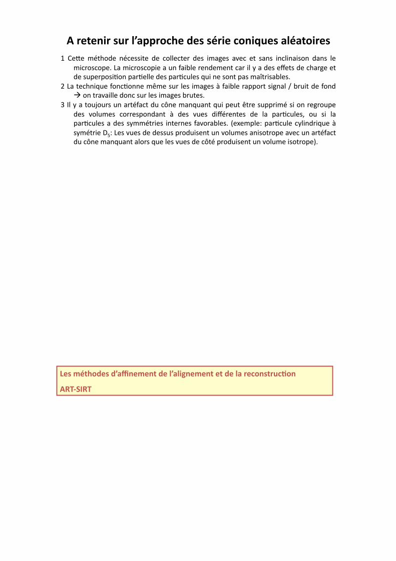
!(6'<'"+6(&76($*#55642>'()'&(&16+'(24"+O7'&(#$1#<4+6'&(
N% V$)$%,:8+"@$% 0:-$''&8$% @$% -"99$-8$#% @$'% &,/7$'% /C$-% $8% '/0'% &0-9&0/&'"0% @/0'% 9$%
,&-#"'-">$E%F/%,&-#"'-">&$%/%=0%4/&(9$%#$0@$,$08%-/#%&9%.%/%@$'%$g$8'%@$%-+/#7$%$8%
@$%'=>$#>"'&?"0%>/#?$99$%@$'%>/#?-=9$'%<=&%0$%'"08%>/'%,/}8#&'/(9$'E%
b%F/%8$-+0&<=$%4"0-?"00$%,W,$%'=#%9$'%&,/7$'%;%4/&(9$%#/>>"#8%'&70/9%x%(#=&8%@$%4"0@%
!%"0%8#/C/&99$%@"0-%'=#%9$'%&,/7$'%(#=8$'E%
c%69%.%/%8"=T"=#'%=0%/#8:4/-8%@=%-|0$%,/0<=/08%<=&%>$=8%W8#$%'=>>#&,:%'&%"0%#$7#"=>$%
@$'% C"9=,$'% -"##$'>"0@/08% ;% @$'% C=$'% @&g:#$08$'% @$% 9/% >/#?-=9$'P% "=% '&% 9/%
>/#?-=9$'%/%@$'%'.,,:8#&$'% &08$#0$'% 4/C"#/(9$'E% K$J$,>9$t%>/#?-=9$%-.9&0@#&<=$%;%
'.,:8#&$%qOt%F$'%C=$'%@$%@$''='%>#"@=&'$08%=0%C"9=,$'%/0&'"8#">$%/C$-%=0%/#8:4/-8%
@=%-|0$%,/0<=/08%/9"#'%<=$%9$'%C=$'%@$%-|8:%>#"@=&'$08%=0%C"9=,$%&'"8#">$LE%
Q'&(,1<>4)'&()*#T"','"<()'($*#$+-"','"<('<()'($#(6'24"&<67234"(
!HL?0UHL(

3$<=&#$%/%#$4$#$0-$%cq%,"@$9E%
3$/9%'>/-$%t%%k+/&S+%lEP%m/"P%nEP%5/J8$#PoElEP%1'8=#&/'P%XEpEP%5"&''$8P%fEP%F$&8+P%1EP%/0@%X#/0SP%pE%KbUU[L%kh6qr3%&,/7$%>#"-$''&07%4"#%
'&079$Q>/#?-9$%#$-"0'8#=-?"0%"4%(&"9"7&-/9%,/-#","9$-=9$'%4#",%$9$-8#"0%,&-#"7#/>+'%,*-./"&0/(-(1(#2&c%KNbL%
N_iNQN_`iE%kh6qr3%'"~u/#$%
h$0-z$SP%hE1EP%m#/''=--&P%3E1EP%X#/0SP%pE%KN__iL%l+$%#&("'",$%/8%&,>#"C$@%#$'"9=?"0t%0$u%8$-+0&<=$'%4"#%,$#7&07%
/0@%"#&$08/?"0%#$G0$,$08%&0%cq%-#."Q$9$-8#"0%,&-#"'-">.%"4%(&"9"7&-/9%>/#?-9$'E%9#-/*)$1/(21('8%ECt%bON�b`UE%
k>&@$#%'"~u/#$%
X"=#&$#%8#/0'4"#,t%
m#&7"#&$gP%fE%KN__[LE%l+#$$Q@&,$0'&"0/9%'8#=-8=#$%"4%("C&0$%f1qnt%=(&<=&0"0$%"J&@"#$@=-8/'$%K-",>9$J%6L%/8%bb%1%
&0%&-$E%34&<(#4&6$(#4%.FFP%NUcc�NUiaE%
p"0&-P%kEP%k"#z/0"P%VE]EP%l+$C$0/zP%hEP%r9Q5$zP%VEP%q$%V/#9"P%kE%Ä%Y0'$#P%!E%KbUUOLE%k>9&0$Q(/'$@%&,/7$Q8"QC"9=,$%
#$7&'8#/?"0%4"#%8+#$$Q@&,$0'&"0/9%$9$-8#"0%,&-#"'-">.E%Y98#/,&-#"'-">.%@VCKiLP%cUcQN`E%
3/@"0%8#/0'4"#,t%3/@$#,/-+$#P%!E%KN__iLE%l+#$$Q@&,$0'&"0/9%#$-"0'8#=-?"0%4#",%
#/0@",%>#"T$-?"0't%"#&$08/?"0/9%/9&70,$08%C&/%3/@"0%8#/0'4"#,'E%9#-/*)$1/(21('8(ECt%NbN�NcaE%
o/C$9$8%8#/0'4"#,t%k"#z/0"P%VE]EP%p"0&-P%kEP%r9Q5$zP%VEP%V/#/z"P%pE!EP%q$%V/#9"P%kEP%l+$C$0/zP%hE%Ä%Y0'$#P%!E%
KbUUiLE%1%,=9?#$'"9=?"0%/>>#"/-+%8"%"#&$08/?"0%/''&70,$08%&0%cq%$9$-8#"0%,&-#"'-">.%"4%'&079$%>/#?-9$'E%p%
k8#=-8%5&"9%@DWKcLP%c[NQ_bE%
h"9/#%X"=#&$#%8#/0'4"#,t%5/S$#P%lEkE%Ä%V+$07P%3EnE%KN__aLE%1%,"@$9Q(/'$@%/>>#"/-+%4"#%@$8$#,&0&07%
"#&$08/?"0'%"4%(&"9"7&-/9%,/-#","9$-=9$'%&,/7$@%(.%-#."$9$-8#"0%,&-#"'-">.E%p%k8#=-8%5&"9%@@WKNLP%NbUQcUE%
k"~u/#$t%%kh6qr3P%6!1m6VP%A!6hhP%r!1fP%$8-E%
K'<>4)&(I46(6'B"','"<(4I(#$+-",'"<(#")(6'24"&<67234"%%
K'<>4)&(<>#<(O7#"3X'(<>'(#$+-",'"<(5#6#,'<'6&(8@9(
!"#$%&'($
)&*'$%&'($
q&#$-8%/)#&(=?"0%"4%r=9$#%/079$'%8"%8+$%
$J>$#&,$08/9%&,/7$'%(.%-",>/#&'"0%
u&8+%bq%>#"T$-?"0'%"4%/%9"u$#Q
#$'"9=?"0P%#$4$#$0-$%C"9=,$E%%
H'I'6'"2'(564N'234"&%K>#"T$-?"0'%"4%/%#$4$#$0-$%C"9=,$P%
@&'-#$8$%0=,($#%"4%>#"T$-?"0%@&#$-?"0'L%

K'<>4)&(<>#<(O7#"3X'(<>'(#$+-",'"<(5#6#,'<'6&(8.9(
]0$%"4%8+$%79"(/9%#$G0$,$08%'8#/8$7&$'E%
r7$9,/0%bUUUP%Y98#/,&-#"'-">.P%[Ot%bbOQbciE%
Y$4M#$(6'B"','"<%
107=9/#%'/,>9&07%'8$>%4"#%
-",>=8/?"0%"4%8+$%9&(#/#.%"4%
#$4$#$0-$%>#"T$-?"0'%&'%
#$@=-$@%&0%$/-+%&8$#/?"0%"4%8+$%
#$G0$,$08E%
!7<6'&(,1<>4)'&()'(6'24"&<67234"()*7"(,4)R$'(561$+,+"#+6'(C/(
FH/>>#"-+$%@$'%9&70$'%-",,=0$'P%'&0"7#/,,$'P%8#/0'4"#,:$%@$%3/@"0%

Q#(,1<>4)'()'&($+-"'&(24,,7"'&(8:$'"#(Z6$4[#(:K\Z(.VVC9(
4 orientations du GroEL-GroES
Les projections 2D correspondantes
Transformée de
Fourier 3D.
Lorsque toutes
directions de l’espace
sont représentées, la
transformée inverse
produit un volume de
reconstruction 3D
isotrope.
Les transformées de Fourier 2D
zzz%r/-+%bq%8#/0'4"#,%&'%/%
-$08#/9%'$-?"0%"4%8+$%cq%
8#/0'4"#,%"4%8+$%"(T$-8E%%
%k"%$/-+%>/&#%"4%bq%
8#/0'4"#,'%+/'%/%-",,"0%
9&0$%
./((((((((((@/(
Projection 2D
(&
00&
3600&
Le « sinogram » d’une
image 2D correspond à l’empilement de ses
différentes projections 1D (lignes) dans
toutes les directions
(0° à 360°).
y
(&
00 ) ( ) 3600&
00&
3600&

Les lignes communes en espace réel:
La méthode des lignes communes
est basée sur le fait que :
N’importe quelle paire de projections
2D d’un objet 3D a au moins une
ligne commune dans leurs
projections 1D respectives.
Projections Views

Image 3 Image 1 900 2700
3100
1300
C5 D5

!(6'<'"+6(&76($*#55642>'()'&($+-"'&(24,,7"'&((
'<()'&(&+"4-6#,,'&(
N%V$)$%,:8+"@$%>$#,$8%@$%-"99$-8$#%@$'%&,/7$'%'/0'%&0-9&0/&'"0%@/0'%9$%,&-#"'-">$E%
b%F$'%'&0"7#/,,$'%0$%,/#-+$08%<=$%'=#%@$'%&,/7$'%;%4"#8%#/>>"#8%'&70/9%x%(#=&8%@$%4"0@%
!%"0%8#/C/&99$%@"0-%'=#%@$'%,".$00$'%bq%
c%F$%-$08#$%@$%,/''$%@$'%,".$00$'%bq%@"&8%-"Z0-&@$#%/C$-%9$%>&J$9%-$08#/9%@$'%&,/7$'E%
F$% >9='% >$?8% @:-/9/7$% &08#"@=&8% =0% (&/&'% @/0'% 9/% @:8$#,&0/?"0% @$'% 9&70$'%
-",,=0$'E%
i%F/%'8#=-8=#$%cq%@H=0$%>/#?-=9$%>#"@=&8$%>/#%-$)$%/>>#"-+$%/%=0$%-+/0-$%'=#%@$=J%
@HW8#$%9$%,/=C/&'%:0/0?","#>+$E%69%4/=8%@"0-%#:/9&'$#%/=%,"&0'%=0$%4"&'%=0$%>/&#$%
@$%>#&'$'%@$%C=$'%/C$-%9$%>"#8$Q"(T$8%&0-9&0:%;%U\%$8%;%NOÅcU\%>"=#%C:#&G$#%<=H"0%/%
(&$0%>#"@=&8%9$%("0%:0/0?",I#$E%
O%F/%8$-+0&<=$%,/#-+$%@H/=8/08%,&$=J%<=$%9/%>/#?-=9$%>"''I@$%@$'%'.,:8#&$'%&08$#0$'E%
L4,4-6#5>+'(1$'2<64"+O7'(2'$$7$#+6'(

l%
L4,4-6#5>+'(2'$$7$#+6'(
q"=(9$%?98%+"9@$#%q"=(9$%?98%+"9@$#%

r9$-8#"0%l","7#/>+.%"4%S&0$8"-+"#$'%
3$-"0'8#=-?"0%"4%m"97&%

!&-#"'-">&$%:9$-8#"0&<=$%%
V$%<=H&9%4/=8%#$8$0&#%Q%
Q"J476O74+(73$+&'6(2'<(473$](
F/%-#."Q,&-#"'-">&$%
Q1C/08/7$t%$0C&#"00$,$08%0/8=#$9%60-"0C$0&$08t%>$=%@$%-"08#/'8$P%$8%8#$'%4#/7&9$%%
K4/&(9$%@"'$%0:-$''/&#$L%
Q"H1&4$734"%%
%w=$99$'%'"08%9$'%9&,&8/?"0'%>"=#%"(8$0&#%=0$%#:'"9=?"0%:9$C:$Ç%
%K,&-#"'-">$'%>$=%>$#4"#,/08P%/($##/?"0%@=%!rP%:-+/0?99"0%>/'%8#$'%+","7$0$L%
Q'&(,1<>4)'&(5476(#$+-"'6()#"&($'&(./('<(6'24"&<7+6'()#"&($'&(C/(7"([4$7,'(
Q@&7&8/9&'$#%9H&,/7$%%$-+/0?99"0/7$%$8%<=/0?G-/?"0%0"#,/9&'/?"0%
V$08#/7$%#$4$#$0-$%4#$$%,=9?#$4$#$0-$%
V9/''&G-/?"0%sQ,$/0%
3$-"0'8#=-?"0%@H=0%,"@$9$%cqE%
!$8+"@$%@$'%'$#&$'%-"0&<=$'%/9$/8"&$%
Q'&0"7#/,,$%
Q3/G0$,$08%@$%9/%'8#=-8=#$%cqP%5/-S%>#"T$-?"0P%13l%k63l%