Embed Size (px)
Citation preview

TelecommunicationsRadar
Courseware Sample
28923-F0
�


TELECOMMUNICATIONSRADAR
COURSEWARE SAMPLE
bythe Staff
ofLab-Volt (Quebec) Ltd
Copyright © 2001 Lab-Volt Ltd
All rights reserved. No part of this publication may bereproduced, in any form or by any means, without the priorwritten permission of Lab-Volt Quebec Ltd.
Printed in CanadaApril 2004
III
��������������
Introduction . . . . . . . . . . . . . . . . . . . . . . . . . . . . . . . . . . . . . . . . . . . . . . . . . V
Courseware Outline
Principles of Radar Systems . . . . . . . . . . . . . . . . . . . . . . . . . . . . . . . . . VII
Analog MTI Processing . . . . . . . . . . . . . . . . . . . . . . . . . . . . . . . . . . . . . . X
Digital MTD Processing . . . . . . . . . . . . . . . . . . . . . . . . . . . . . . . . . . . . . XII
Tracking Radar . . . . . . . . . . . . . . . . . . . . . . . . . . . . . . . . . . . . . . . . . . . XIV
Radar in an Active Target Environment . . . . . . . . . . . . . . . . . . . . . . . . . XVI
The Phased Array Antenna . . . . . . . . . . . . . . . . . . . . . . . . . . . . . . . . . . XIX
Sample Exercise from Principles of Radar Systems
Ex. 2-3 The PPI Display . . . . . . . . . . . . . . . . . . . . . . . . . . . . . . . . . . . . . 3
The generation and use of the PPI display. Markers. Measuring therange and angular resolution using the PPI display.
Sample Exercise from Analog MTI Processing
Ex. 1-3 Staggered PRF . . . . . . . . . . . . . . . . . . . . . . . . . . . . . . . . . . . . 33
Blind speeds. Second-trace echoes and range ambiguities. The effectof staggered PRF on blind speeds and second-trace echoes. Thefrequency response of a single delay-line canceller in staggered PRFmode.
Sample Exercise from Digital MTD Processing
Ex. 3-2 Surveillance (Track-While-Scan) Processing . . . . . . . . . . . . . . 71
Processing steps used in surveillance processing. Track scoring.
Sample Exercise from Tracking Radar
Ex. 3 Angle Tracking Techniques . . . . . . . . . . . . . . . . . . . . . . . . . . . . 83
Lobe switching technique. Crossover loss. Conical scan technique.Monopulse technique. Advantages of the monopulse technique overthe lobe switching and conical scan techniques. Lobe switchingimplementation in the Lab-Volt tracking radar.
��������������� ������
IV
Sample Exercise from Radar in an Active Target Environment
Ex. 3-1 Deceptive Jamming UsingAmplitude-Modulated Signals . . . . . . . . . . . . . . . . . . . . . . . . . 109
The principles of inverse gain jamming as used against conical scanand sequential lobing angular tracking systems. Distinction betweenasynchronous/synchronous inverse gain jamming and AM noise. Theimportance of lobing/scanning rate agility as a radar EP againstamplitude-modulation angle deception techniques.
Sample Exercise from The Phased Array Antenna
Ex. 1-1 Basic Principles, Operation and Adjustment . . . . . . . . . . . . . . 129
Setting up and operating the PAA with the Digital Radar System.
Other samples extracted from Principles of Radar Systems
Unit Test . . . . . . . . . . . . . . . . . . . . . . . . . . . . . . . . . . . . . . . . . . . . . . . 135
Instructor’s Guide Sample Extract from Principles of Radar Systems
Unit 2 A Pulsed Radar System . . . . . . . . . . . . . . . . . . . . . . . . . . . . 139
Bibliography
V
��������
The Lab-Volt Radar Training System, Model 8095, is a modular table-top radarsystem especially designed for teaching radar in a laboratory classroom. It is a realradar system, not a simulator, that uses innovative technology to detect passivetargets at very short ranges. The low-power of its transmitter allows safe operationin a variety of training environments.
The Radar Training System can operate as a pulsed, continuous wave (CW), orfrequency-modulated continuous wave (FM-CW) radar. When operated as a pulsedradar, the A-scope and plan position indicator (PPI) displays are available. Only afew connections and adjustments are required to rapidly pass from the hands-onstudy of a pulsed radar to that of a CW or FM-CW radar.
The design of the Radar Training System emphasizes functionality, with blockdiagrams silk-screened on the module front panels. Major inputs and outputs arereadily accessible through various connectors on the front panels. For certaininstructional modules, test points are brought out to the front panel, whereas forothers, they are located on the printed circuit board. In this case, they are accessedthrough a hinged door located on top of the module. All test points and outputs areshort-circuit protected.
Faults can be inserted by the instructor in the instructional modules, for teachingtroubleshooting, using the fault switches located on the printed circuit boards ofthese modules. These switches are accessed through the hinged door located ontop of each instructional module. Another hinged panel inside each of thesemodules prevents students from accessing the fault switches.
The student courseware for the Radar Training System consists of four volumesand a set of additional exercises. The courseware covers the following subjectmatter:
– The first volume, titled Principles of Radar Systems, deals with the principlesand operation of pulsed, CW, and FM-CW radars.
– A second volume, titled Analog MTI Processing, covers the principles of analogsignal processing and MTI radar.
– The next volume in the series, titles Digital MTD Processing, presents moderndigital processing techniques related to those used in air-traffic-control radars.
– The last volume in the series, titled Tracking Radar, explains the principles ofoperation of tracking radars (with emphasis on the lobe-switching trackingradar) and discusses the factors which may affect the range and angle trackingperformance.
– The additional exercises make use of the capability of the Radar TrainingSystem to perform various radar measurements of fundamental parameters,particularly radar cross sections.
An instructor’s guide is also available. This guide provides outlines of the theorypresented in the courseware, and describes many demonstrations that, in mostcases, have not been included in the student manuals. These demonstrations area useful complement to radar teaching. The instructor’s guide also provides aids tothe presentation of the various topics covered in the courseware.

����������� ������
VI
The Unit-Exercise structure of the radar courseware is similar to that used in thecourseware for the Analog and Digital Communications Training Systems. Each unitof instruction consists of several exercises designed to present material inconvenient instructional segments. Principles and concepts are presented first, andhands-on procedures complete the learning process to involve and better acquaintthe student with each module, and with complete radar systems.
At the end of each exercise, there is a five-questions review section requiring briefwritten answers. Suggested answers for these questions, as well as for those foundin the exercise procedures, are included in the appendices of the student manuals.Each unit terminates with a ten-question multiple-choice test to verify the knowledgegained in the unit. The answers for these questions are given in the radarinstructor’s guide only.
PRINCIPLES OF RADAR SYSTEMS
����������������
VII
Unit 1 Fundamentals of Pulsed Radar
The fundamentals of pulsed radar, including the range-delayrelationship, radar antennas, and the radar equation, as well as safetymeasures applicable to all radar systems.
Ex. 1-1 Basic Principles of Pulsed Radar
Basic principles of pulsed radar. Introduction to the RadarTraining System and the A-scope display. Safety measuresapplicable to all radar systems.
Ex. 1-2 The Range-Delay Relationship
The relationship between target range and the delay betweenpulse transmission and echo reception. The concept of rangeresolution. Measuring target range and range resolutionusing the A-scope display.
Ex. 1-3 Radar Antennas
The role of the antenna in a radar system. Radar antennacharacteristics. Plotting the radiation pattern and measuringangular resolution of the radar antenna.
Ex. 1-4 The Radar Equation
The various parameters in the radar equation and theirinteraction in a radar system.
Unit 2 A Pulsed Radar System
The transmitter, the receiver, the antenna driving system, the PPIdisplay, and the PPI scan converter in a pulsed radar system.
Ex. 2-1 Radar Transmitter and Receiver
The operating principles of a pulsed radar transmitter andreceiver. The Radar Transmitter and Radar Receiver of theRadar Training System.
Ex. 2-2 Antenna Driving System
The mechanical aspects and control of a rotating or scanningradar antenna.
PRINCIPLES OF RADAR SYSTEMS
����������������
VIII
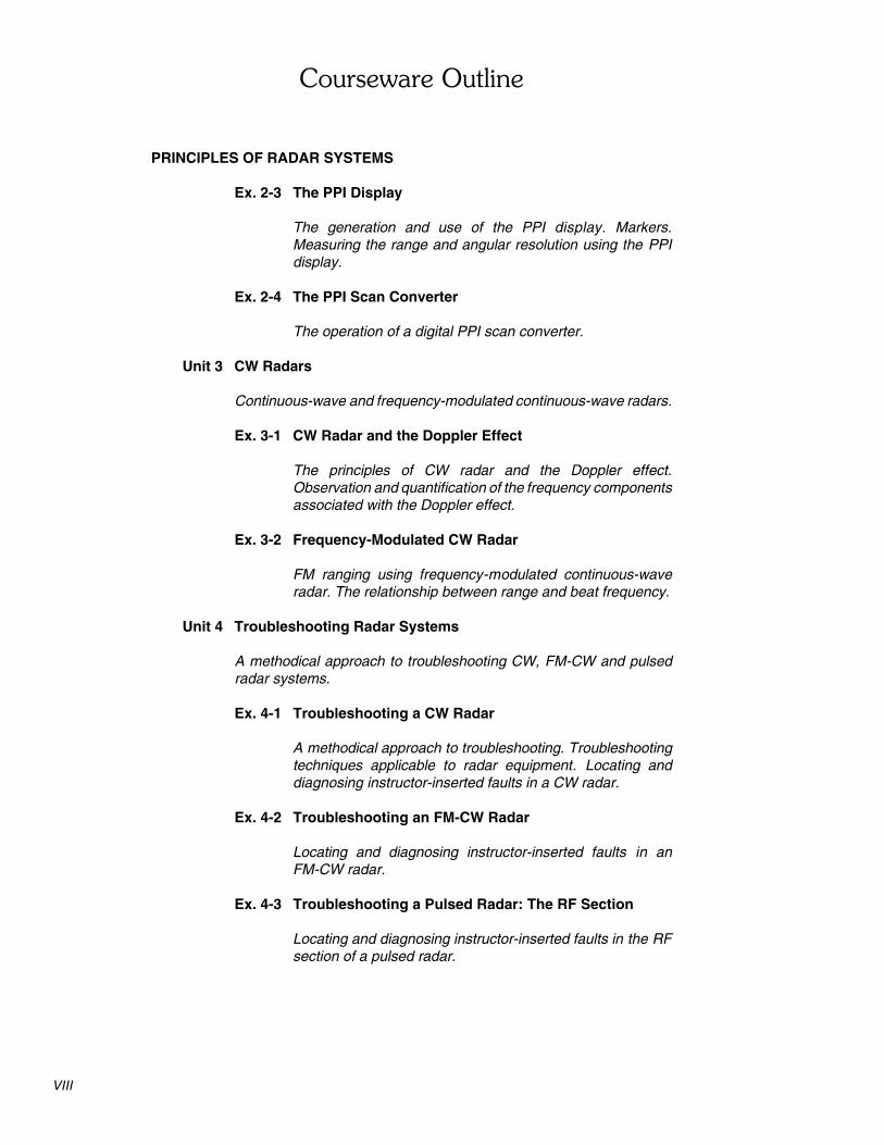
Ex. 2-3 The PPI Display
The generation and use of the PPI display. Markers.Measuring the range and angular resolution using the PPIdisplay.
Ex. 2-4 The PPI Scan Converter
The operation of a digital PPI scan converter.
Unit 3 CW Radars
Continuous-wave and frequency-modulated continuous-wave radars.
Ex. 3-1 CW Radar and the Doppler Effect
The principles of CW radar and the Doppler effect.Observation and quantification of the frequency componentsassociated with the Doppler effect.
Ex. 3-2 Frequency-Modulated CW Radar
FM ranging using frequency-modulated continuous-waveradar. The relationship between range and beat frequency.
Unit 4 Troubleshooting Radar Systems
A methodical approach to troubleshooting CW, FM-CW and pulsedradar systems.
Ex. 4-1 Troubleshooting a CW Radar
A methodical approach to troubleshooting. Troubleshootingtechniques applicable to radar equipment. Locating anddiagnosing instructor-inserted faults in a CW radar.
Ex. 4-2 Troubleshooting an FM-CW Radar
Locating and diagnosing instructor-inserted faults in anFM-CW radar.
Ex. 4-3 Troubleshooting a Pulsed Radar: The RF Section
Locating and diagnosing instructor-inserted faults in the RFsection of a pulsed radar.

PRINCIPLES OF RADAR SYSTEMS
����������������
IX
Ex. 4-4 Troubleshooting a Pulsed Radar: The PPI ScanConverter
Locating and diagnosing instructor-inserted faults in thedisplay section of a pulsed radar.
Appendices A Setting Up the Radar Training SystemB Calibration of the Radar DisplaysC Targets and Radar Cross SectionD Operation of the Dual-Channel SamplerE Common SymbolsF Module Front PanelsG Test Points and DiagramsH Answers to Procedure Step QuestionsI Answers to Review QuestionsJ Index of New TermsK Equipment Utilization Chart
BibliographyReader’s Comment Form
ANALOG MTI PROCESSING
����������������
X
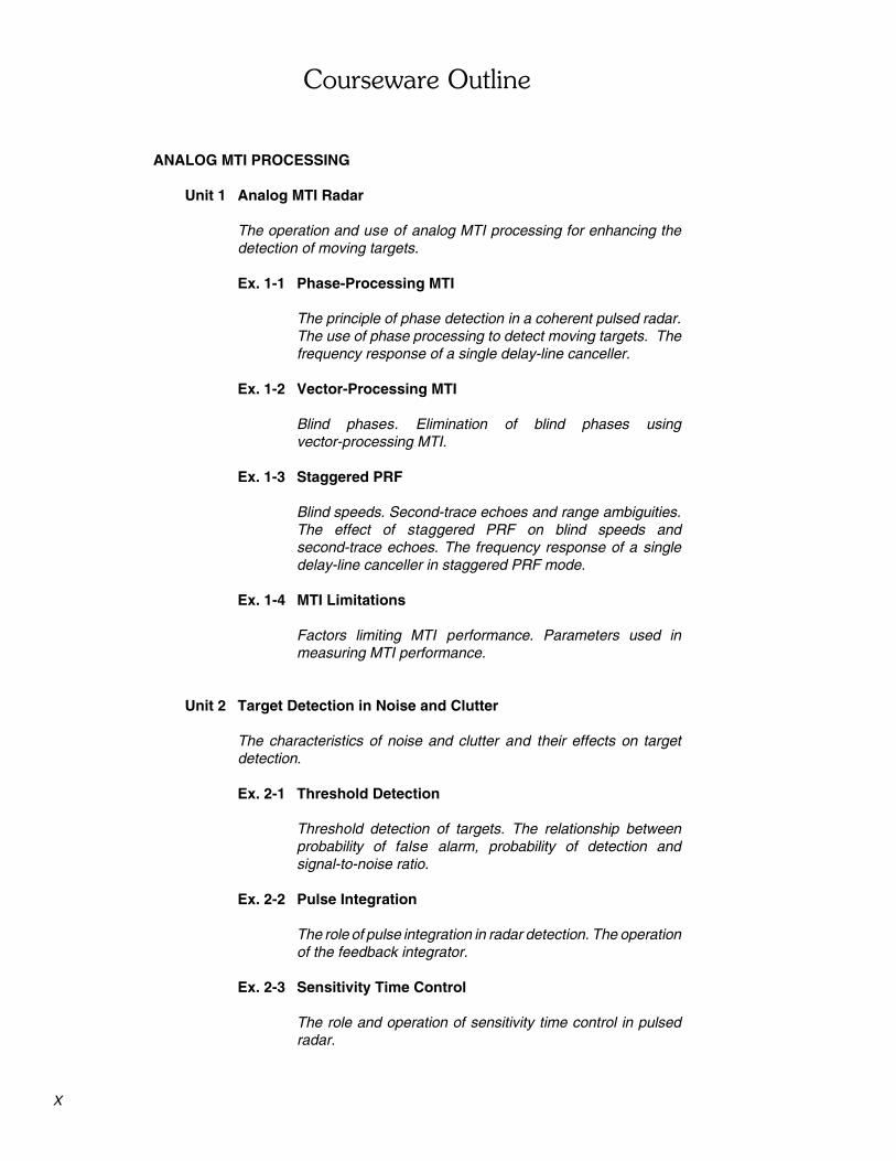
Unit 1 Analog MTI Radar
The operation and use of analog MTI processing for enhancing thedetection of moving targets.
Ex. 1-1 Phase-Processing MTI
The principle of phase detection in a coherent pulsed radar.The use of phase processing to detect moving targets. Thefrequency response of a single delay-line canceller.
Ex. 1-2 Vector-Processing MTI
Blind phases. Elimination of blind phases usingvector-processing MTI.
Ex. 1-3 Staggered PRF
Blind speeds. Second-trace echoes and range ambiguities.The effect of staggered PRF on blind speeds andsecond-trace echoes. The frequency response of a singledelay-line canceller in staggered PRF mode.
Ex. 1-4 MTI Limitations
Factors limiting MTI performance. Parameters used inmeasuring MTI performance.
Unit 2 Target Detection in Noise and Clutter
The characteristics of noise and clutter and their effects on targetdetection.
Ex. 2-1 Threshold Detection
Threshold detection of targets. The relationship betweenprobability of false alarm, probability of detection andsignal-to-noise ratio.
Ex. 2-2 Pulse Integration
The role of pulse integration in radar detection. The operationof the feedback integrator.
Ex. 2-3 Sensitivity Time Control
The role and operation of sensitivity time control in pulsedradar.
ANALOG MTI PROCESSING
����������������
XI
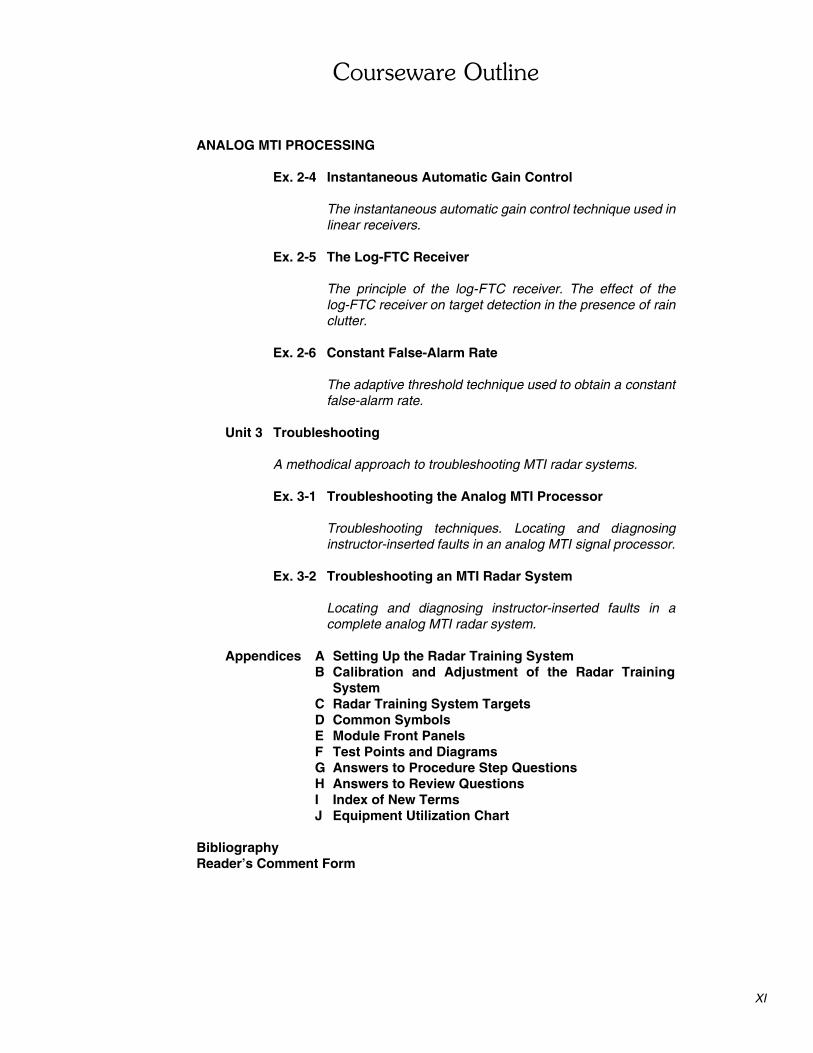
Ex. 2-4 Instantaneous Automatic Gain Control
The instantaneous automatic gain control technique used inlinear receivers.
Ex. 2-5 The Log-FTC Receiver
The principle of the log-FTC receiver. The effect of thelog-FTC receiver on target detection in the presence of rainclutter.
Ex. 2-6 Constant False-Alarm Rate
The adaptive threshold technique used to obtain a constantfalse-alarm rate.
Unit 3 Troubleshooting
A methodical approach to troubleshooting MTI radar systems.
Ex. 3-1 Troubleshooting the Analog MTI Processor
Troubleshooting techniques. Locating and diagnosinginstructor-inserted faults in an analog MTI signal processor.
Ex. 3-2 Troubleshooting an MTI Radar System
Locating and diagnosing instructor-inserted faults in acomplete analog MTI radar system.
Appendices A Setting Up the Radar Training SystemB Calibration and Adjustment of the Radar Training
SystemC Radar Training System TargetsD Common SymbolsE Module Front PanelsF Test Points and DiagramsG Answers to Procedure Step QuestionsH Answers to Review QuestionsI Index of New TermsJ Equipment Utilization Chart
BibliographyReader’s Comment Form
DIGITAL MTD PROCESSING
����������������
XII
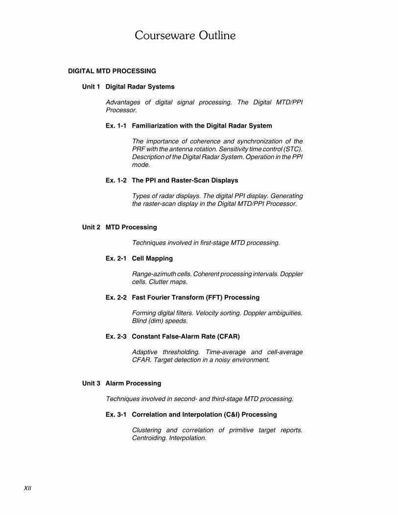
Unit 1 Digital Radar Systems
Advantages of digital signal processing. The Digital MTD/PPIProcessor.
Ex. 1-1 Familiarization with the Digital Radar System
The importance of coherence and synchronization of thePRF with the antenna rotation. Sensitivity time control (STC).Description of the Digital Radar System. Operation in the PPImode.
Ex. 1-2 The PPI and Raster-Scan Displays
Types of radar displays. The digital PPI display. Generatingthe raster-scan display in the Digital MTD/PPI Processor.
Unit 2 MTD Processing
Techniques involved in first-stage MTD processing.
Ex. 2-1 Cell Mapping
Range-azimuth cells. Coherent processing intervals. Dopplercells. Clutter maps.
Ex. 2-2 Fast Fourier Transform (FFT) Processing
Forming digital filters. Velocity sorting. Doppler ambiguities.Blind (dim) speeds.
Ex. 2-3 Constant False-Alarm Rate (CFAR)
Adaptive thresholding. Time-average and cell-averageCFAR. Target detection in a noisy environment.
Unit 3 Alarm Processing
Techniques involved in second- and third-stage MTD processing.
Ex. 3-1 Correlation and Interpolation (C&I) Processing
Clustering and correlation of primitive target reports.Centroiding. Interpolation.
DIGITAL MTD PROCESSING
����������������
XIII
Ex. 3-2 Surveillance (Track-While-Scan) Processing
Processing steps used in surveillance processing. Trackscoring.
Unit 4 Troubleshooting
A methodical approach to troubleshooting.
Ex. 4-1 Troubleshooting the Digital MTD/PPI Processor
Locating and diagnosing instructor-inserted faults in theDigital MTD/PPI Processor.
Appendices A Setting Up the Radar Training SystemB Setting Up and Connecting the ModulesC Calibrating the Digital Radar Training SystemD FunctionsE Radar Training System TargetsF Common SymbolsG Module Front PanelH Test Points and DiagramsI Answers to Procedure Step Questions
BibliographyReader's Comment Form
TRACKING RADAR
����������������
XIV
Exercise 1 Manual Tracking of a Target
What is a tracking radar? Track-while-scan (TWS) radar versuscontinuous tracking radar. Manual tracking of a target. Rangegate, range gate marker, and O-scope display. Manual control ofthe antenna and range gate positions in the Lab-Volt trackingradar.
Exercise 2 Automatic Range Tracking
Principle of automatic range tracking. Applications of rangetrackers. Target search and acquisition. Split range-gate tracking.Leading-edge range tracking and trailing-edge range tracking.Range tracking rate limitation. Operation of the range tracker inthe Lab-Volt tracking radar.
Exercise 3 Angle Tracking Techniques
Lobe switching technique. Crossover loss. Conical scantechnique. Monopulse technique. Advantages of the monopulsetechnique over the lobe switching and conical scan techniques.Lobe switching implementation in the Lab-Volt tracking radar.
Exercise 4 Automatic Angle Tracking
Principle of automatic angle tracking. Operation of the angletracker in the Lab-Volt tracking radar.
Exercise 5 Range and Angle Tracking Performance(Radar-Dependent Errors)
Resolution, precision, and accuracy of tracking radars. Radar-dependent errors. Effect of the receiver thermal noise and antennaservosystem noise and limitations on the tracking error. Use of anAGC circuit to reduce the variation of the echo amplitude due tofluctuations of the target radar cross section.
TRACKING RADAR
����������������
XV
Exercise 6 Range and Angle Tracking Performance(Target-Caused Errors)
Amplitude scintillation. Effect of the amplitude scintillation on theangular tracking error in lobe switching and conical scan trackingradars. Angular scintillation (glint). Effect of the angular scintillationon the angular tracking error. Principle of frequency agility. Use offrequency agility to reduce the angular tracking error.
Exercise 7 Troubleshooting an Analog Target Tracker
Use of a methodical approach to locate and diagnose instructor-inserted faults in the Radar Target Tracker.
Appendices A Setting Up the Radar Training SystemB Calibration and Adjustment of the Tracking Radar
Training SystemC Answers to Procedure Step QuestionsD Answers to Review Questions
BibliographyReader's Comment Form
RADAR IN AN ACTIVE TARGET ENVIRONMENT
����������������
XVI
Unit 1 Noise Jamming . . . . . . . . . . . . . . . . . . . . . . . . . . . . . . . . . . . . . . . 1-1
The context of electronic warfare in modern conflicts. Introduction toelectronic warfare and its subdivisions (EA, EP, ES). The relationshipbetween the subdivisions.
Ex. 1-1 Familiarization with the Radar Jamming Pod . . . . . . . . 1-7
Familiarization with the various controls, input/output connectors,and accessories on the Radar Jamming Pod. Radar JammingPod properties and jamming signal capabilities.
Ex. 1-2 Spot Noise Jamming and Burn-Through Range . . . . . 1-23
Description of spot noise jamming. Difference between the self-screening, mutual-support, escort, and stand-off EA missions.The concept of burn-through range. Introduction of the radarrange equation modified for spot noise jamming.
Ex. 1-3 Frequency Agility and Barrage Noise Jamming . . . . . 1-39
Discussion relating to the radar receiver passband. Introductionto frequency agility as an electronic protection against spot noisejamming. Description of barrage noise jamming. Justification ofthe use of barrage noise jamming against frequency-agile radars.Swept spot jamming as used with the Radar Jamming Pod.
Ex. 1-4 Video Integration and Track-On-Jamming . . . . . . . . . . 1-57
The importance of signal discrimination (signal processingtechniques) used as radar EPs against noise jamming. A caseexample, the effects of video integration when used by a radarconfronted with noise jamming. Discussion of the jammer strobe.The angle track-on jamming capability of certain radars.
Ex. 1-5 Antennas in EW: Sidelobe Jammingand Space Discrimination . . . . . . . . . . . . . . . . . . . . . . 1-81
Presentation of the difference between mainlobe and sidelobejamming. Outline of the effects of effective sidelobe noisejamming. Presentation of certain antenna space discriminationtechniques used as radar EP against stand-off noise jammers.

RADAR IN AN ACTIVE TARGET ENVIRONMENT
����������������
XVII
Unit 2 Range Deception Jamming . . . . . . . . . . . . . . . . . . . . . . . . . . . . . 2-1
The fundamental differences between noise jamming and deceptionjamming. Presentation of the different categories of deceptive jamming.Comparison between range deception and angle deception jammingtechniques.
Ex. 2-1 Deception Jamming using the Radar Jamming Pod . . 2-3
Generating false targets with the Radar Jamming Pod.Familiarization with the RGPO and the on-off modulationcapabilities of the Jamming Pod.
Ex. 2-2 Range Gate Pull-Off . . . . . . . . . . . . . . . . . . . . . . . . . . . 2-19
The implementation of range DECM against radars that use splitrange-gate tracking. Introduction to range gate pull-off (RGPO),and the phases of an RGPO jamming cycle. Use of a range-ratetracking limiter as an EP against unrealistic RGPO. Use ofleading-edge range tracking as an EP against RGPO.
Ex. 2-3 Stealth Technology: The Quest for Reduced RCS . . . 2-35
Introduction to the basic material and design principles behindradar stealth technology. The role of hard-body shaping andradar absorbent materials (RAM) in the implementation of theseprinciples. Implications of stealth technology to electronicwarfare.
Unit 3 Angle Deception Jamming . . . . . . . . . . . . . . . . . . . . . . . . . . . . . . 3-1
Reasons that angle and range DECM are implemented together againsttracking radars. Differentiation between those angle deception techniquesused against conical scanning and sequential lobing radars, and thoseused against monopulse radars. Introduction to silent lobing as an EP.
Ex. 3-1 Deceptive Jamming UsingAmplitude-Modulated Signals . . . . . . . . . . . . . . . . . . . . 3-5
The principles of inverse gain jamming as used against conicalscan and sequential lobing angular tracking systems. Distinctionbetween asynchronous/synchronous inverse gain jamming andAM noise. The importance of lobing/scanning rate agility as aradar EP against amplitude-modulation angle deceptiontechniques.
RADAR IN AN ACTIVE TARGET ENVIRONMENT
����������������
XVIII
Ex. 3-2 Cross-Polarization Jamming . . . . . . . . . . . . . . . . . . . . . 3-23
The main reason for the existence of the cross-polarized(Condon lobes) antenna radiation pattern. Comparison betweentypical parabolic antenna cross- and co-polarized antennapatterns. Introduction to cross-polarization jamming.
Ex. 3-3 Multiple-Source Jamming Techniques . . . . . . . . . . . . . 3-45
The mutual support EA mission and its relation to cooperativejamming techniques. How multiple-source jamming techniquesinduce artificial glint onto the jamming signal. Distinction betweencoherent and incoherent multiple-source jamming. The differencebetween formation and blinking jamming, and how victim radarsuse angle-rate limiters as electronic protection.
Unit 4 Chaff . . . . . . . . . . . . . . . . . . . . . . . . . . . . . . . . . . . . . . . . . . . . . . . . 4-1
Fundamentals of chaff physics, and reasons why the Lab-Volt variable-density chaff cloud (VDCC) reproduces the effects of chaff. Dispensingand uses of chaff. Chaff placed within its historical context.
Ex. 4-1 Chaff Clouds . . . . . . . . . . . . . . . . . . . . . . . . . . . . . . . . . . 4-5
Corridor dispensing of chaff. Discrimination of chaff echoes usingradar MTI processing. Setting-up the Lab-Volt variable-densitychaff cloud (VDCC).
Ex. 4-2 Chaff Clouds used as Decoys . . . . . . . . . . . . . . . . . . . . 4-17
Burst dispensing of chaff to create false targets. Introduction tojammer-illuminated chaff (JAFF). Defeating the processing abilityof MTI radars via the noisy Doppler frequency imparted to chaffclouds via JAFF.
Appendices A Setting Up the Radar Training SystemB Calibration and Adjustment of the Tracking Radar Training
SystemC Answers to Procedure Step QuestionsD Answers to Review QuestionsE Glossary
BibliographyWe Value Your Opinion!
THE PHASED ARRAY ANTENNA
����������������
XIX
Unit 1 Basic Operation
Ex. 1-1 Basic Principles, Operation and Adjustments
Setting up and operating the PAA with the Digital Radar System.
Ex. 1-2 The True-Time Delay Rotman Lens
Principles of the Rotman lens.
Ex. 1-3 The Switching Matrix
Operation of the RF switching matrix.
Unit 2 Measurement of Useful Phased Array Antenna Characteristics
Ex. 2-1 Beamwidth Measurement
Measuring the 3 dB beamwidth of the PAA.
Ex. 2-2 Radiation Pattern Measurement
Measuring the PAA radiation pattern and plotting the radiationpattern from your results.
Ex. 2-3 Angular Separation Measurement
Measuring the angular separation between two consecutive PAAbeams.
Ex. 2-4 Phased Array Antenna Gain Measurement
Measuring the PAA gain for various beams (center and far end).PAA gain versus scan angle.
Ex. 2-5 Maximum Scan Angle Measurement
Measuring the maximum scan angle of the PAA.
Ex. 2-6 Target Bearing Estimation
Target position relative to a selected beam.
THE PHASED ARRAY ANTENNA
����������������
XX
Ex. 2-7 Target Speed Estimation
Calculating the speed of a target moving perpendicularly to theradar line of sight, using the angular displacement and the scanspeed to estimate the target speed.
Appendices A Set-up and adjustment of the PAA with the Analog RadarB Set-up and adjustment of the PAA with the Digital RadarC Answers to Procedure Step QuestionsD Answers to Review QuestionsE GlossaryF Equipment Utilization Chart
BibliographyWe Value Your Opinion!

���������������
����
�������������������� �����

3
0°
BLIP
BEARING Þ
R
RANGE
ORIGIN
�����������
������ ��������
EXERCISE OBJECTIVE
When you have completed this exercise, you will be familiar with the generation anduse of the PPI display and with the various markers available on the display. Youwill also be able to measure the range and angular resolution of a radar systemusing the PPI display.
Note: This exercise can be performed using either the Analog Radar TrainingSystem or the Complete Radar Training System. Both of these systemsinclude the PPI Scan Converter.
DISCUSSION
Indicators and displays are used in radar systems to present information about thetargets in a suitable form. When only the target range and echo signal strength areimportant, the A-scope display is usually used. This is often the case when theantenna is fixed in one particular direction.
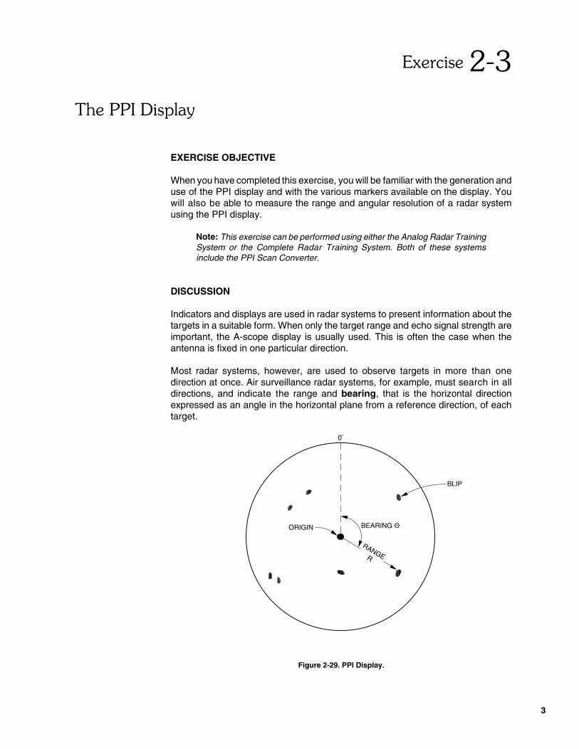
Most radar systems, however, are used to observe targets in more than onedirection at once. Air surveillance radar systems, for example, must search in alldirections, and indicate the range and bearing, that is the horizontal directionexpressed as an angle in the horizontal plane from a reference direction, of eachtarget.
Figure 2-29. PPI Display.
�!������"�����
4
0°
Þ
R
ORIGIN
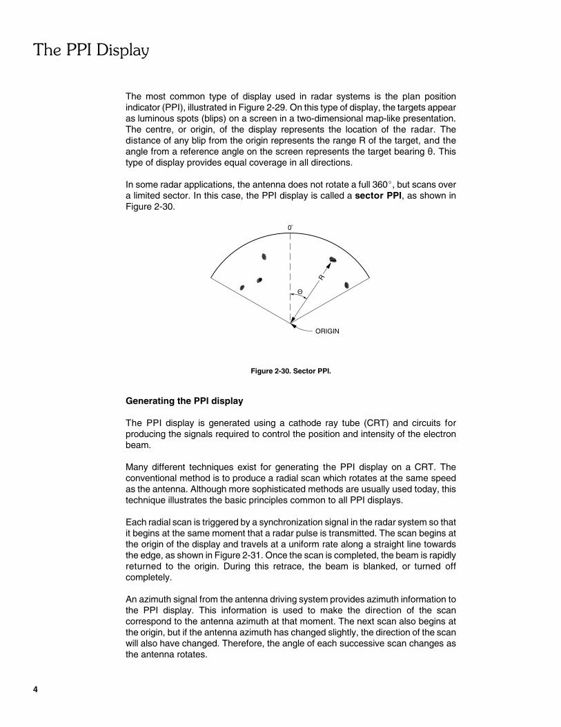
The most common type of display used in radar systems is the plan positionindicator (PPI), illustrated in Figure 2-29. On this type of display, the targets appearas luminous spots (blips) on a screen in a two-dimensional map-like presentation.The centre, or origin, of the display represents the location of the radar. Thedistance of any blip from the origin represents the range R of the target, and theangle from a reference angle on the screen represents the target bearing �. Thistype of display provides equal coverage in all directions.
In some radar applications, the antenna does not rotate a full 360�, but scans overa limited sector. In this case, the PPI display is called a sector PPI, as shown inFigure 2-30.
Figure 2-30. Sector PPI.
Generating the PPI display
The PPI display is generated using a cathode ray tube (CRT) and circuits forproducing the signals required to control the position and intensity of the electronbeam.
Many different techniques exist for generating the PPI display on a CRT. Theconventional method is to produce a radial scan which rotates at the same speedas the antenna. Although more sophisticated methods are usually used today, thistechnique illustrates the basic principles common to all PPI displays.
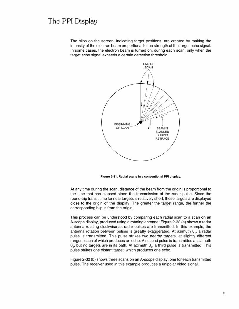
Each radial scan is triggered by a synchronization signal in the radar system so thatit begins at the same moment that a radar pulse is transmitted. The scan begins atthe origin of the display and travels at a uniform rate along a straight line towardsthe edge, as shown in Figure 2-31. Once the scan is completed, the beam is rapidlyreturned to the origin. During this retrace, the beam is blanked, or turned offcompletely.
An azimuth signal from the antenna driving system provides azimuth information tothe PPI display. This information is used to make the direction of the scancorrespond to the antenna azimuth at that moment. The next scan also begins atthe origin, but if the antenna azimuth has changed slightly, the direction of the scanwill also have changed. Therefore, the angle of each successive scan changes asthe antenna rotates.
�!������"�����
5
END OFSCAN
BEGINNINGOF SCAN BEAM IS
BLANKEDDURING
RETRACE
The blips on the screen, indicating target positions, are created by making theintensity of the electron beam proportional to the strength of the target echo signal.In some cases, the electron beam is turned on, during each scan, only when thetarget echo signal exceeds a certain detection threshold.
Figure 2-31. Radial scans in a conventional PPI display.
At any time during the scan, distance of the beam from the origin is proportional tothe time that has elapsed since the transmission of the radar pulse. Since theround-trip transit time for near targets is relatively short, these targets are displayedclose to the origin of the display. The greater the target range, the further thecorresponding blip is from the origin.
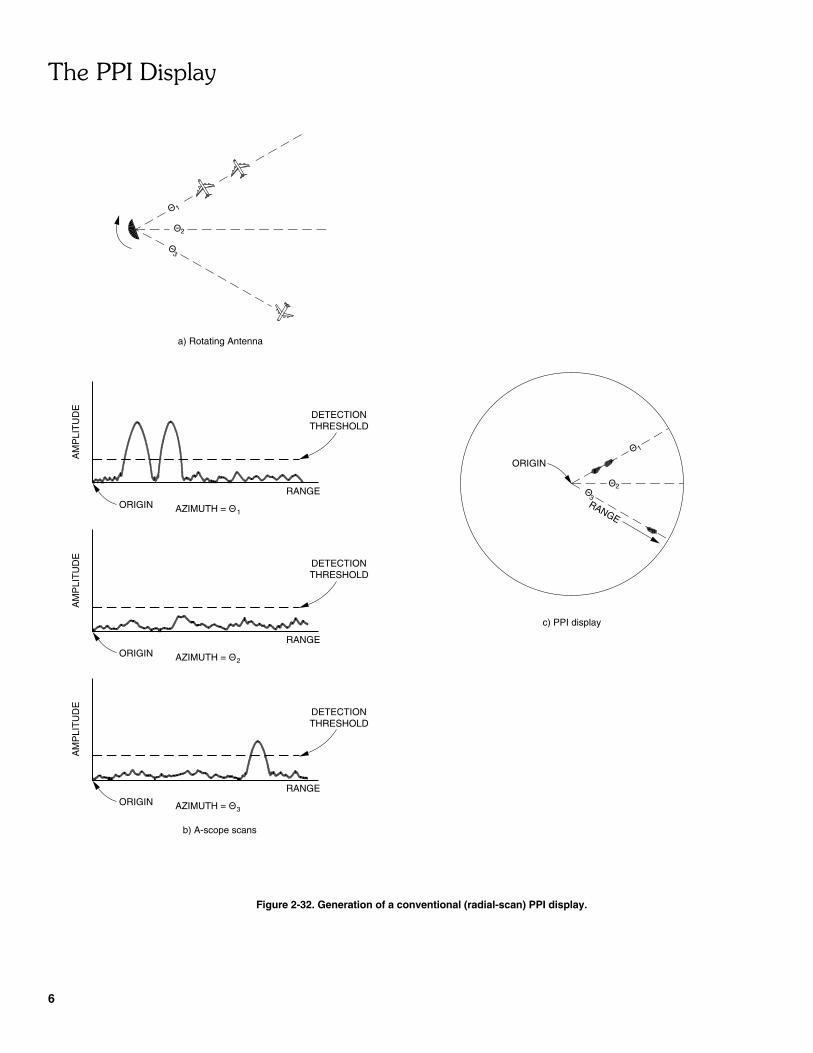
This process can be understood by comparing each radial scan to a scan on anA-scope display, produced using a rotating antenna. Figure 2-32 (a) shows a radarantenna rotating clockwise as radar pulses are transmitted. In this example, theantenna rotation between pulses is greatly exaggerated. At azimuth �1, a radarpulse is transmitted. This pulse strikes two nearby targets, at slightly differentranges, each of which produces an echo. A second pulse is transmitted at azimuth�2, but no targets are in its path. At azimuth �3, a third pulse is transmitted. Thispulse strikes one distant target, which produces one echo.
Figure 2-32 (b) shows three scans on an A-scope display, one for each transmittedpulse. The receiver used in this example produces a unipolar video signal.
�!������"�����
6
Þ1
2Þ
Þ3
a) Rotating Antenna
AZIMUTH = Þ1
AM
PLI
TU
DE
ORIGINRANGE
DETECTIONTHRESHOLD
AM
PLI
TU
DE
AZIMUTH = ÞORIGIN2
THRESHOLD
RANGE
DETECTION
RANGE
AZIMUTH = ÞORIGIN3
AM
PLI
TU
DE
THRESHOLDDETECTION
b) A-scope scans
c) PPI display
ORIGIN
RANGE
Þ2
3Þ
Þ1
Figure 2-32. Generation of a conventional (radial-scan) PPI display.
�!������"�����
7
Two echoes are received at azimuth �1, one for each target. Since the echoes arereceived at slightly different times, they produce two distinct blips on the display asthe electron beam scans from left (the origin) to right. Both of these echoes exceedthe detection threshold.
At azimuth �2, some noise is present, but the noise does not exceed the detectionthreshold.
At azimuth �3, one echo exceeds the detection threshold. Since this echocorresponds to a distant target, the blip appears to the right of the display.
Figure 2-32 (c) shows how these three scans would appear on a PPI display. Thescan at angle �1 begins at the origin and moves towards the edge. The electronbeam, however, is off. When the first echo exceeds the detection threshold, thebeam turns on producing a blip on the PPI display. The beam stays on as long asthe echo pulse amplitude is greater than the detection threshold, then it turns off.As this scan continues towards the edge of the screen, it is again turned on by thesecond echo, producing a second blip.
Since no echo is received while the antenna azimuth is equal to �2, the beam is notturned on during the second scan. During the third scan, at angle �3, the beam isturned on once.
This example shows that each radial scan on a PPI display, from the origin to theedge, is comparable to a scan on an A-scope display. The blips on the PPI screenare created by turning the electron beam on whenever the target echo signalexceeds the detection threshold. In both displays, the distance of the blip from theorigin represents the target range.
In a practical radar system, the antenna may rotate only a fraction of a degreebetween transmitted pulses. As a result, each target is illuminated by many pulses,rather than by just one, as in the example.
Many modern radars convert the radial-scan display into a raster-scan format similarto television. This allows the display to be produced on a TV-type monitor. Theoverall appearance of the PPI display, however, is not changed.
Markers
Besides the blips corresponding to the targets detected, many PPI displays candisplay various types of markers which help the operator to determine the rangesand bearings of the targets. Controls on the display usually allow the markers to beturned on or off.
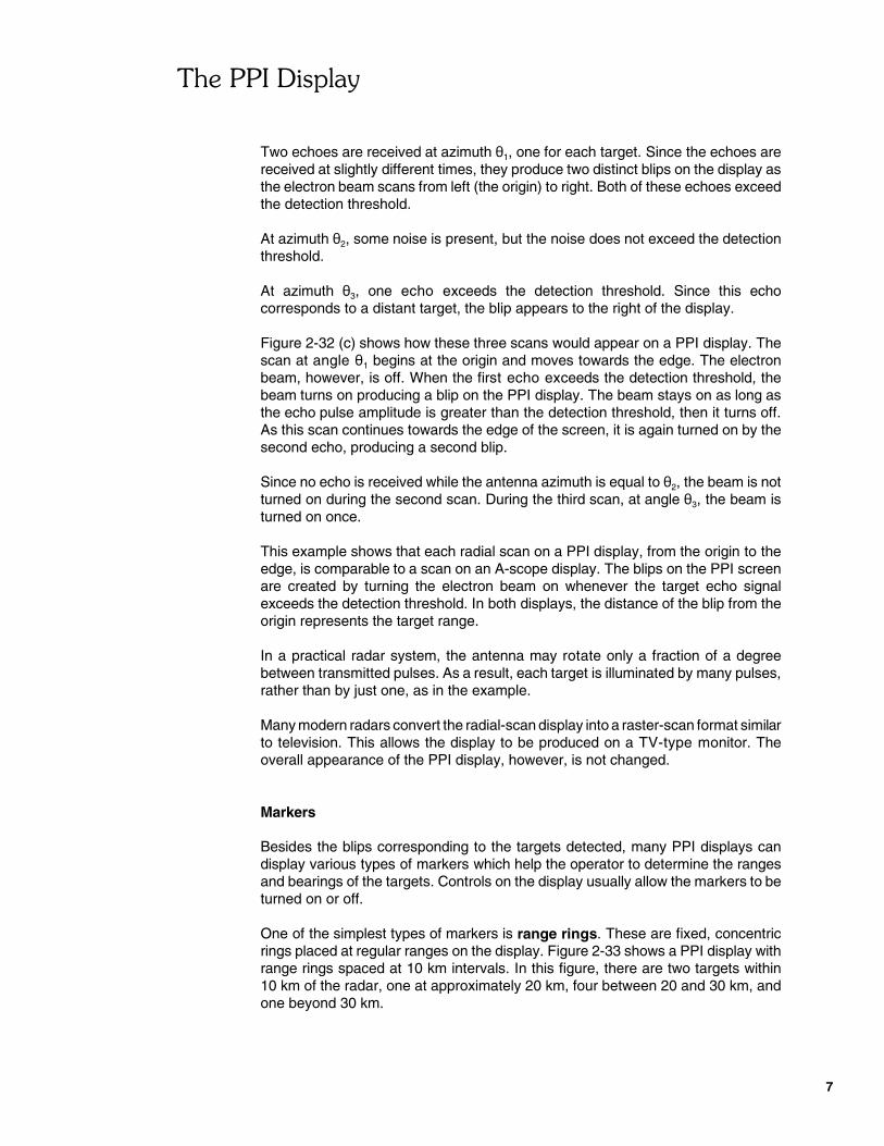
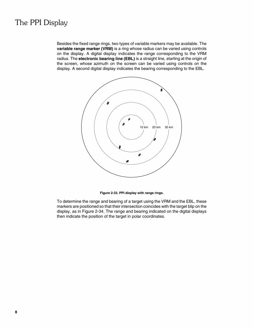
One of the simplest types of markers is range rings. These are fixed, concentricrings placed at regular ranges on the display. Figure 2-33 shows a PPI display withrange rings spaced at 10 km intervals. In this figure, there are two targets within10 km of the radar, one at approximately 20 km, four between 20 and 30 km, andone beyond 30 km.
�!������"�����
8
10 km 20 km 30 km
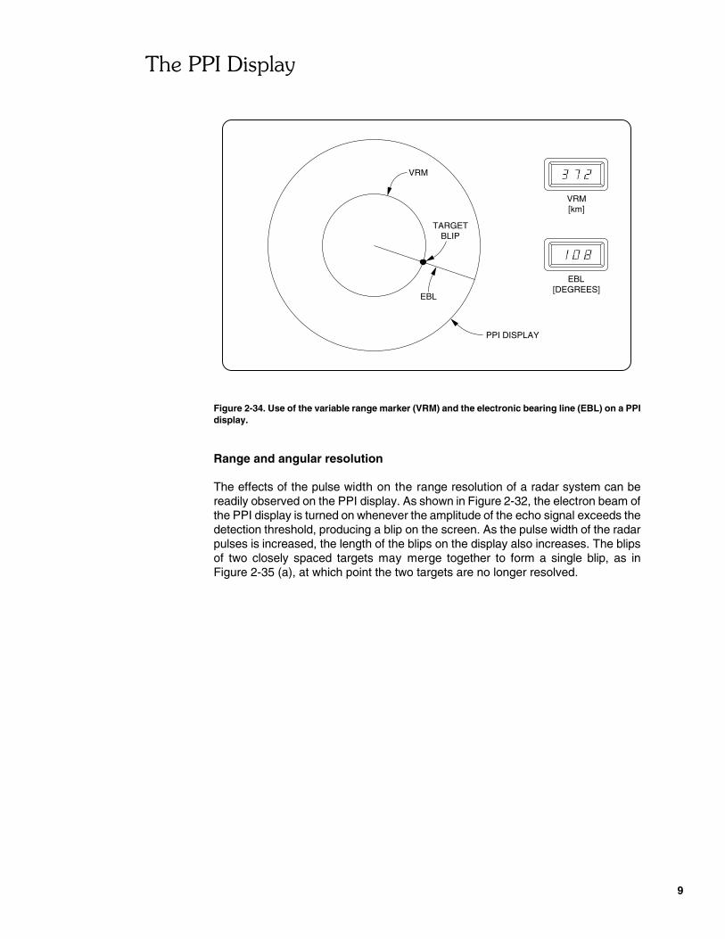
Besides the fixed range rings, two types of variable markers may be available. Thevariable range marker (VRM) is a ring whose radius can be varied using controlson the display. A digital display indicates the range corresponding to the VRMradius. The electronic bearing line (EBL) is a straight line, starting at the origin ofthe screen, whose azimuth on the screen can be varied using controls on thedisplay. A second digital display indicates the bearing corresponding to the EBL.
Figure 2-33. PPI display with range rings.
To determine the range and bearing of a target using the VRM and the EBL, thesemarkers are positioned so that their intersection coincides with the target blip on thedisplay, as in Figure 2-34. The range and bearing indicated on the digital displaysthen indicate the position of the target in polar coordinates.
�!������"�����
9
VRM[km]
EBL[DEGREES]
VRM
TARGETBLIP
PPI DISPLAY
EBL
Figure 2-34. Use of the variable range marker (VRM) and the electronic bearing line (EBL) on a PPIdisplay.
Range and angular resolution
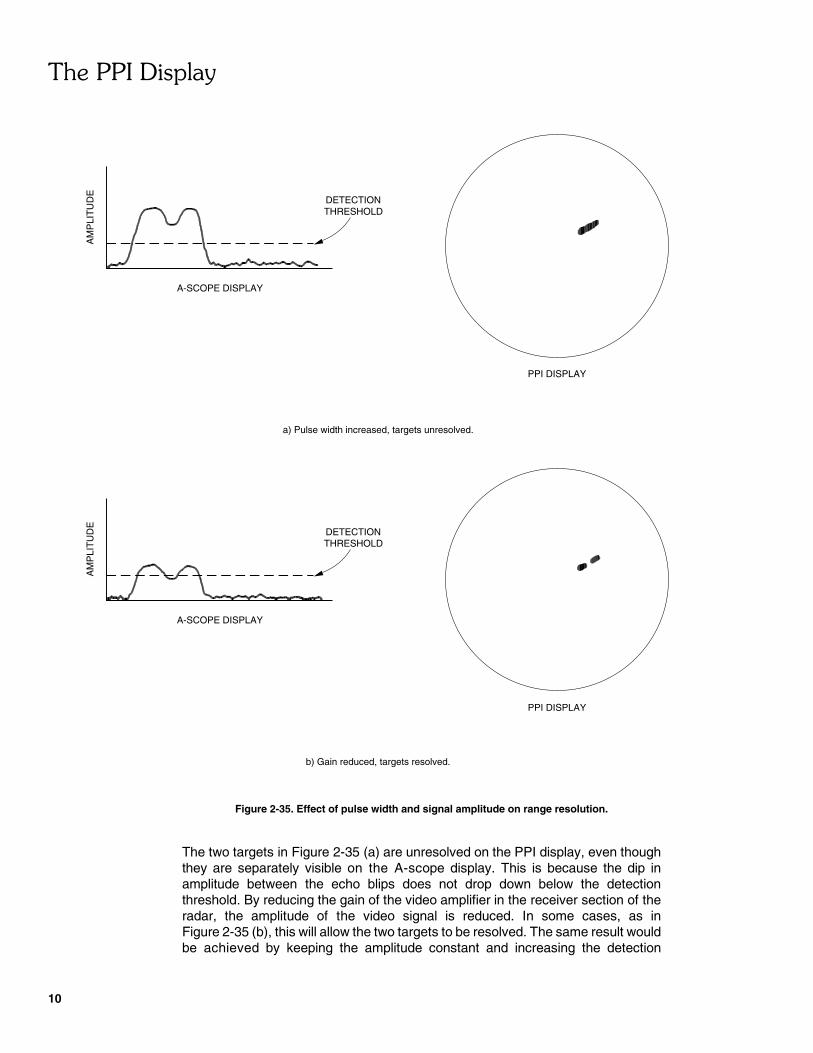
The effects of the pulse width on the range resolution of a radar system can bereadily observed on the PPI display. As shown in Figure 2-32, the electron beam ofthe PPI display is turned on whenever the amplitude of the echo signal exceeds thedetection threshold, producing a blip on the screen. As the pulse width of the radarpulses is increased, the length of the blips on the display also increases. The blipsof two closely spaced targets may merge together to form a single blip, as inFigure 2-35 (a), at which point the two targets are no longer resolved.
�!������"�����
10
a) Pulse width increased, targets unresolved.
A-SCOPE DISPLAY
AM
PLI
TU
DE
DETECTIONTHRESHOLD
THRESHOLDDETECTION
AM
PLI
TU
DE
A-SCOPE DISPLAY
PPI DISPLAY
PPI DISPLAY
b) Gain reduced, targets resolved.
Figure 2-35. Effect of pulse width and signal amplitude on range resolution.
The two targets in Figure 2-35 (a) are unresolved on the PPI display, even thoughthey are separately visible on the A-scope display. This is because the dip inamplitude between the echo blips does not drop down below the detectionthreshold. By reducing the gain of the video amplifier in the receiver section of theradar, the amplitude of the video signal is reduced. In some cases, as inFigure 2-35 (b), this will allow the two targets to be resolved. The same result wouldbe achieved by keeping the amplitude constant and increasing the detection
�!������"�����
11
threshold. Most radar systems have a gain control which can be adjusted foroptimum resolution.
As was discussed in Unit 1, the theoretical range resolution of a pulsed radar isequal to one half the pulse length:
Theoretical range resolution �
Lp
2
�� c2
where Lp is the pulse length� is the pulse widthc is the speed of light.
The angular resolution of a radar system can also be observed using the PPIdisplay. Two targets at the same range but at different bearings will appear as twodistinct blips if they are resolved. The angular resolution depends mostly on theantenna beamwidth. As in the case of range resolution, optimum angular resolutiondepends on correct adjustment of the gain and the detection threshold.
As stated in Unit 1, the angular resolution is usually between 1 and 1.5 times theantenna 3-dB beamwidth.
Procedure Summary
In the first part of this exercise, you will set up a pulsed radar including a PPIdisplay. The block diagram of the system you will use is shown in Figure 2-37. Theconnection of the oscilloscope is not shown in this figure since it is required duringadjustment of the pulsed radar.
In the second part of this exercise, you will carry out the adjustment of the dc offsetvoltages at the SAMPLED OUTPUTS of the Dual-Channel Sampler. Thisadjustment will prevent undesired dc offset voltages from saturating the PPI display.
In the third part of this exercise, you will calibrate the origin of the PPI display. Thiswill allow you to learn the operation and use of a VRM, since you will use the VRMof the PPI Scan Converter to calibrate the PPI display.
In the fourth part of this exercise, you will learn the operation and use of othermarkers by using the RANGE RINGS and EBL of the PPI Scan Converter. You willuse the VRM and the EBL to determine the polar coordinates of various blips on thePPI display, and then try to find which objects in the laboratory classroomcorrespond to these blips. You will observe the effect that the range of observationhas on the position of blips on the PPI display, by selecting two different ranges ofobservation.
In the fifth part of this exercise, you will measure the angular resolution of the pulsedradar using the PPI display, and compare this to the angular resolution expected.
�!������"�����
12
RADAR TRANSMITTER
RADAR RECEIVER
RADAR SYNCHRONIZER/
POWER SUPPLY
ANTENNA CONTROLLER
ANTENNA MOTOR DRIVER
OSCILLOSCOPE
PPI SCAN CONVERTER
ANALOG MTIPROCESSOR
DUAL-CHANNEL SAMPLER
In the sixth part of this exercise, you will observe the effect of the pulse width on theaspect of the blips on the PPI display. You will measure the range resolution of thepulsed radar using the PPI display, and compare this to the theoretical rangeresolution.
PROCEDURE
Setting up a pulsed radar
� 1. The main elements of the Radar Training System, that is the antenna andits pedestal, the target table and the training modules, must be set upproperly before beginning this exercise. Refer to Appendix A of this manualfor setting up the Radar Training System, if this is not done yet.
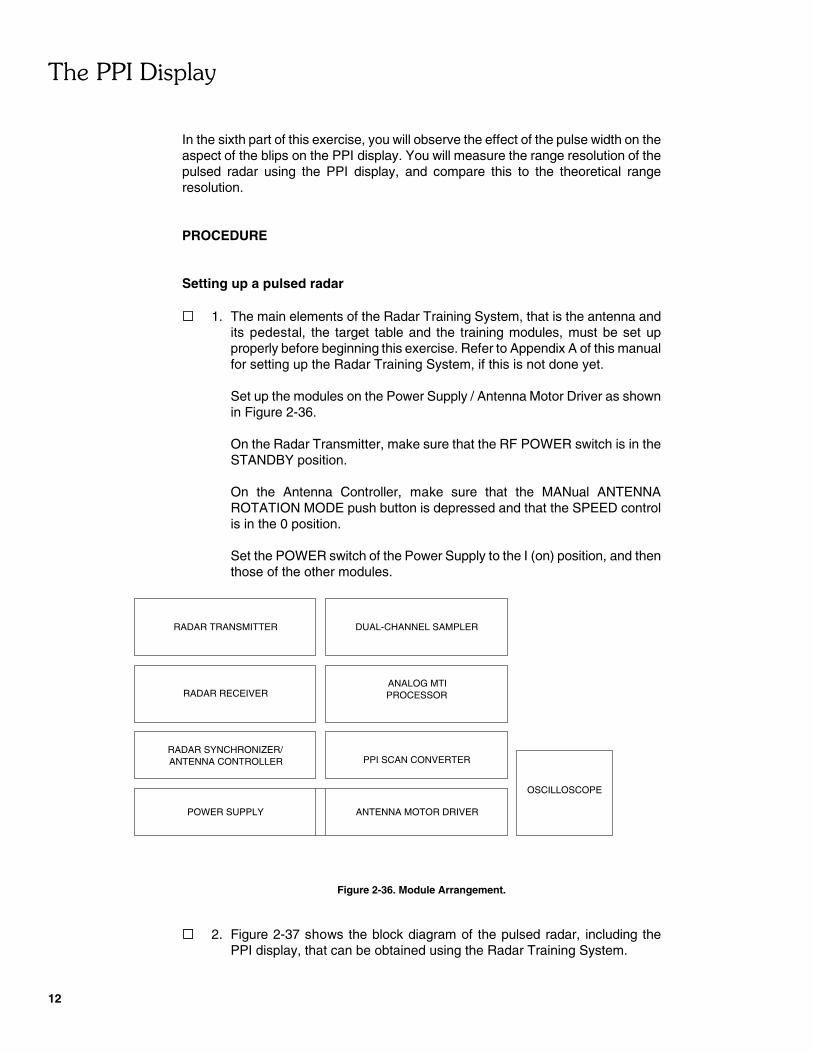
Set up the modules on the Power Supply / Antenna Motor Driver as shownin Figure 2-36.
On the Radar Transmitter, make sure that the RF POWER switch is in theSTANDBY position.
On the Antenna Controller, make sure that the MANual ANTENNAROTATION MODE push button is depressed and that the SPEED controlis in the 0 position.
Set the POWER switch of the Power Supply to the I (on) position, and thenthose of the other modules.
Figure 2-36. Module Arrangement.
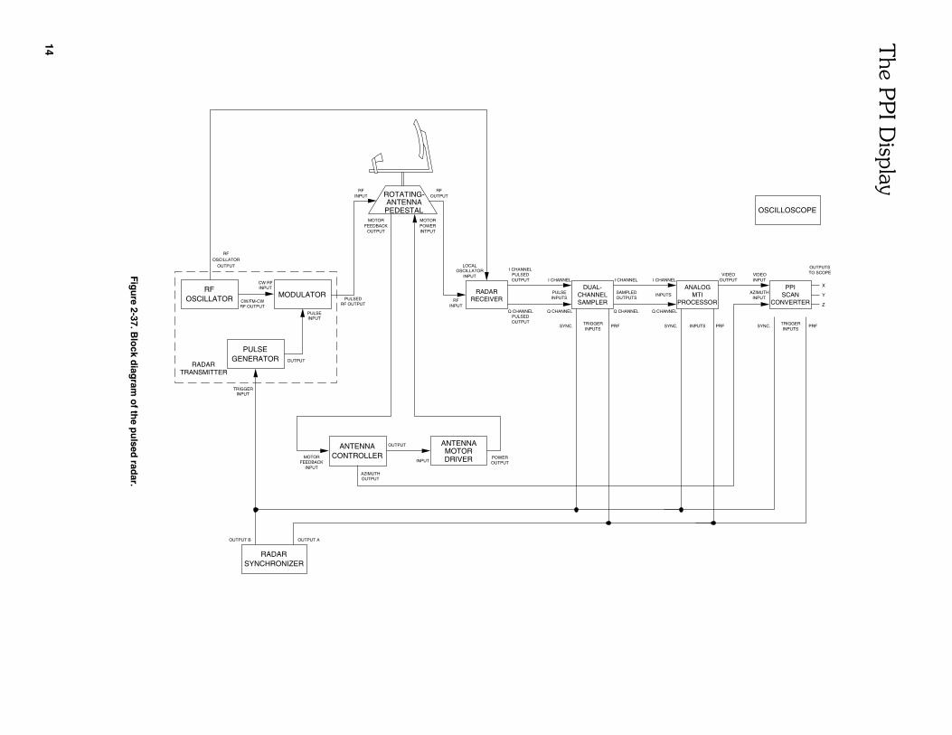
� 2. Figure 2-37 shows the block diagram of the pulsed radar, including thePPI display, that can be obtained using the Radar Training System.
�!������"�����
13
Install a BNC T-connector on OUTPUT B of the Radar Synchronizer, thenconnect the modules according to this block diagram. The connection of theoscilloscope is not shown in Figure 2-37 since it is required duringadjust-ment of the pulsed radar.
Note: The SYNC. TRIGGER INPUT of the Dual-ChannelSampler and the PULSE GENERATOR TRIGGER INPUT of theRadar Transmitter must be connected directly to OUTPUT B ofthe Radar Synchronizer without passing through BNCT-connectors.
� 3. Make the following adjustments:
On the Radar Transmitter
RF OSCILLATOR FREQUENCY . . . . . . . CAL.PULSE GENERATOR PULSE WIDTH . . 1 ns
On the Radar Synchronizer
PRF MODE . . . . . . . . . . . . . . . . . . . . SINGLEPRF . . . . . . . . . . . . . . . . . . . . . . . . . . . 216 Hz
On the Dual-Channel Sampler
ORIGIN . . . . . . . . . . . . . . . . . . Max. clockwise
� 4. On the Antenna Controller, use the SPEED control so that the RadarAntenna rotates at least one turn, then stop it. Depress the POSITIONMODE push button, then use the SPEED control to set the position(azimuth) of the Radar Antenna to approximately 0�.
�!������"
�����
14
INPUT
POWERMOTOR
INTPUT
ROTATING-
PEDESTAL
ANTENNA OUTPUT
OUTPUT B
SYNCHRONIZERRADAR
OUTPUT A
MOTOR
INPUTFEEDBACK
AZIMUTHOUTPUT
CONTROLLER
INPUTTRIGGER
OSCILLATOR
GENERATOR
TRANSMITTERRADAR
OSCILLATORRF
OUTPUT
RF
PULSEOUTPUT
MODULATORCW/FM-CWRF OUTPUT
CW RFINPUT
PULSEINPUT
PULSEDRF OUTPUT
FEEDBACKMOTOR
OUTPUT
INPUTRF
ANTENNA
MOTORDRIVER POWER
OUTPUT
CONVERTERSCAN
INPUTSTRIGGER
OSCILLOSCOPE
INPUTS
ANTENNA
Q CHANNELPULSEDOUTPUT
I CHANNELPULSEDOUTPUT
OSCILLATORINPUT
RFINPUT
RECEIVERRADAR
LOCAL
I CHANNEL
Q CHANNEL
SYNC.
PULSEINPUTS
TRIGGER
SAMPLER
DUAL-CHANNEL
ANALOG
PROCESSOR
INPUTS
Q CHANNEL
I CHANNEL
INPUTS
Q CHANNEL
PRF
I CHANNEL
OUTPUTSSAMPLED
SYNC.
MTI AZIMUTH
PRF
VIDEOOUTPUT
SYNC.
INPUT
INPUTVIDEO
PPI
OUTPUTRF
PRF
Z
TO SCOPE
X
Y
OUTPUTS
Fig
ure 2-37. B
lock d
iagram
of th
e pu
lsed rad
ar.
�!������"�����
15
Y
X
˜ 2.0 m
Connect the cable of the target table to the multi-pin connector located onthe rear panel of the Target Controller. Make sure that the surface of thetarget table is free of any objects and then set the POWER switch of theTarget Positioning System to the I (on) position.
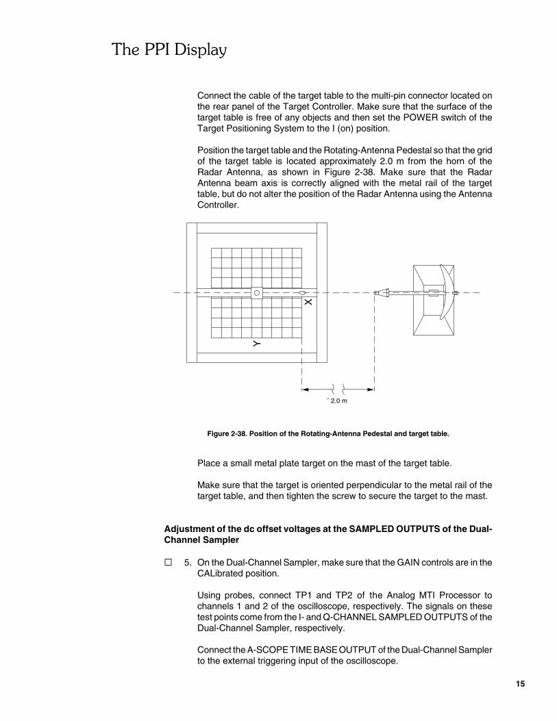
Position the target table and the Rotating-Antenna Pedestal so that the gridof the target table is located approximately 2.0 m from the horn of theRadar Antenna, as shown in Figure 2-38. Make sure that the RadarAntenna beam axis is correctly aligned with the metal rail of the targettable, but do not alter the position of the Radar Antenna using the AntennaController.
Figure 2-38. Position of the Rotating-Antenna Pedestal and target table.
Place a small metal plate target on the mast of the target table.
Make sure that the target is oriented perpendicular to the metal rail of thetarget table, and then tighten the screw to secure the target to the mast.
Adjustment of the dc offset voltages at the SAMPLED OUTPUTS of the Dual-Channel Sampler
� 5. On the Dual-Channel Sampler, make sure that the GAIN controls are in theCALibrated position.
Using probes, connect TP1 and TP2 of the Analog MTI Processor tochannels 1 and 2 of the oscilloscope, respectively. The signals on thesetest points come from the I- and Q-CHANNEL SAMPLED OUTPUTS of theDual-Channel Sampler, respectively.
Connect the A-SCOPE TIME BASE OUTPUT of the Dual-Channel Samplerto the external triggering input of the oscilloscope.
�!������"�����
16
Adjust the oscilloscope as follows:
Channel 1 . . . . . . . . . . . . . 0.2 V/DIV (set to GND)Channel 2 . . . . . . . . . . . . . 0.2 V/DIV (set to GND)Vertical Mode . . . . . . . . . . . . . . . . . . . . . . . . . ALTTime Base . . . . . . . . . . . . . . . . . . . . . . . 1 ms/DIVTrigger . . . . . . . . . . . . . . . . . . . . . . . . . . . . . . EXT
Set the vertical position controls so that the traces of channels 1 and 2 arecentred in the upper and lower halves of the oscilloscope screen,respectively. Set the input coupling switches of both channels to theDC position.
On the Dual-Channel Sampler, set the I- and Q-CHANNEL DC OFFSETcontrols so that there is no noticeable offset voltage at TP1 and TP2 of theAnalog MTI Processor.
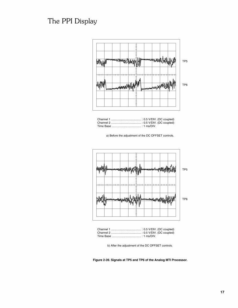
� 6. Disconnect the probes going to channels 1 and 2 of the oscilloscope fromTP1 and TP2 of the Analog MTI Processor, then connect them to TP5 andTP6 of the same module, respectively. The signals on these test points arerelated to channels I and Q, respectively.
On the Analog MTI Processor, place the STC switch in the I (on) positionand depress the 7.2-m RANGE push button. The operation of the controlsof the Analog MTI Processor is covered in Volume 2 of the Radar TrainingSystem.
On the oscilloscope, set the sensitivity of the two channels to anappropriate level. Figure 2-39 (a) shows an example of what you mightobserved on the oscilloscope screen.
On the Dual-Channel Sampler, set the I- and Q-CHANNEL DC OFFSETcontrols so that the signals at TP5 and TP6 of the Analog MTI Processorresembles those shown in Figure 2-39 (b).
This completes the adjustment of the dc offset voltages at the SAMPLEDOUTPUTS of the Dual-Channel Sampler. A generalized procedure is foundin Appendix B of this manual.
�!������"�����
17
TP6
TP5
Channel 1 ...................................... : 0.5 V/DIV. (DC coupled)Channel 2 ...................................... : 0.5 V/DIV. (DC coupled)Time Base ..................................... : 1 ms/DIV.
a) Before the adjustment of the DC OFFSET controls.
b) After the adjustment of the DC OFFSET controls.
Time Base ..................................... : 1 ms/DIV.Channel 2 ...................................... : 0.5 V/DIV. (DC coupled)Channel 1 ...................................... : 0.5 V/DIV. (DC coupled)
TP6
TP5
Figure 2-39. Signals at TP5 and TP6 of the Analog MTI Processor.
�!������"�����
18
Calibration of the PPI display
� 7. Remove the cable and probes connected to the oscilloscope. Connect theX, Y, and Z OUTPUTS TO SCOPE of the PPI Scan Converter tochannels X, Y, and Z of the oscilloscope, respectively.
Make the following adjustments:
On the Analog MTI Processor
RANGE . . . . . . . . . . . . . . . . . . . . . . . . . 3.6 mSTC . . . . . . . . . . . . . . . . . . . . . . . . . . . . . . . OMTI . . . . . . . . . . . . . . . . . . . . . . . . . . . . . . . OIAGC . . . . . . . . . . . . . . . . . . . . . . . . . . . . . . OMODE . . . . . . . . . . . . . . . . . . . . . . . . . . . LIN.VIDEO INTEGRATOR . . . . . . . . . . . . . . . . . OGAIN . . . . . . . . . . . . . . . . . . . . . . . . . . . MIN.
On the PPI Scan Converter
RANGE . . . . . . . . . . . . . . . . . . . . . . . . . 3.6 mRANGE RINGS . . . . . . . . . . . . . . . . . . . . . . OVRM . . . . . . . . . . . . . . . . . . . . . . . . . . . . . . . OEBL . . . . . . . . . . . . . . . . . . . . . . . . . . . . . . . O
On the Dual-Channel Sampler
RANGE SPAN . . . . . . . . . . . . . . . . . . . . 3.6 m
On the oscilloscope
Channel 1 . . . . . . . . . . . 1 V/DIV (DC coupled)Channel 2 . . . . . . . . . . . 1 V/DIV (DC coupled)Time Base . . . . . . . . . . . . . . . . . . . . . . . . X-Y
A circle should appear on the oscilloscope screen. Set the X- and Y-axisposition controls of the oscilloscope so that the circle is centred on thescreen. This circle delimits the area of the PPI display.
� 8. On the Target Controller, make sure that the X- and Y-axis SPEED controlsare in the MINimum position and then make the following settings:
MODE . . . . . . . . . . . . . . . . . . . . . . . . . . . SPEEDDISPLAY MODE . . . . . . . . . . . . . . . . . . . . SPEED
Set the Y-axis SPEED control so that the target speed is equal toapproximately 15 cm/s.
On the Antenna Controller, depress the SPEED MODE push button, selectthe SCANning/TRACKing ANTENNA ROTATION MODE, then set theSPEED control so that the rotation speed of the Radar Antenna is
�!������"�����
19
MOVING TARGET BLIP
Range ........................................................: 3.6 m
approximately 10 r/min. The Radar Antenna should start to scan back andforth in the direction of the moving target.
On the Analog MTI Processor, set the GAIN control to one quarter ofMAXimum. This control varies the level of the video signal sent to theVIDEO INPUT of the PPI Scan Converter.
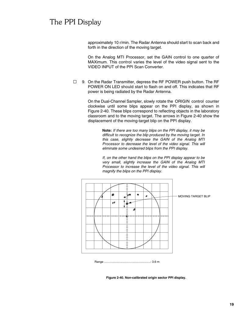
� 9. On the Radar Transmitter, depress the RF POWER push button. The RFPOWER ON LED should start to flash on and off. This indicates that RFpower is being radiated by the Radar Antenna.
On the Dual-Channel Sampler, slowly rotate the ORIGIN control counterclockwise until some blips appear on the PPI display, as shown inFigure 2-40. These blips correspond to reflecting objects in the laboratoryclassroom and to the moving target. The arrows in Figure 2-40 show thedisplacement of the moving-target blip on the PPI display.
Note: If there are too many blips on the PPI display, it may bedifficult to recognize the blip produced by the moving target. Inthis case, slightly decrease the GAIN of the Analog MTIProcessor to decrease the level of the video signal. This willeliminate some undesired blips from the PPI display.
If, on the other hand the blips on the PPI display appear to bevery small, slightly increase the GAIN of the Analog MTIProcessor to increase the level of the video signal. This willmagnify the blips on the PPI display.
Figure 2-40. Non-calibrated origin sector PPI display.

�!������"�����
20
Range ........................................................: 3.6 m
On the Dual-Channel Sampler, continue to rotate the ORIGIN controlcounterclockwise in order to bring the origin of the PPI display nearer to thehorn of the Radar Antenna, until the PPI display resembles that shown inFigure 2-41.
Figure 2-41. A sector PPI display whose origin is too close to the Radar Antenna.
What causes these large blips on the PPI display?
(Hint: see Figure 1-9 of this manual.)
� 10. On the Dual-Channel Sampler, set the ORIGIN control so that the moving-target blip appears on the PPI display.
On the Target Controller, set the Y-axis SPEED to 0, then make thefollowing settings:
MODE . . . . . . . . . . . . . . . . . . . . . . . . . POSITIONDISPLAY MODE . . . . . . . . . . . . . . . . . . POSITION
Use the Y-axis position control to place the target at the far end of thetarget table. The target range is now approximately 2.9 m since the grid ofthe target table is approximately 2.0 m from the horn of the Radar Antenna.

�!������"�����
21
On the PPI Scan Converter, place the VRM switch in the I (on) position toenable the VRM. The range related to the VRM is indicated on theVRM display. Successively depress the + and � push buttons locatedbelow the VRM display while observing the PPI display. Describe the VRM.
What is the main purpose of the VRM?
� 11. On the PPI Scan Converter, use the VRM controls to set the VRM toapproximately 2.9 m. This corresponds to the range of the target installedon the target table.
On the Dual-Channel Sampler, set the ORIGIN control so that the blipcorresponding to the target installed on the target table is centred on theVRM.
On the Antenna Controller, set the SPEED control to 0, then select thePRF LOCKed ANTENNA ROTATION MODE. The Radar Antenna shouldnow rotate clockwise. Figure 2-42 shows an example of what you mightobserve on the PPI display.

�!������"�����
22
Range ........................................................: 3.6 m
TARGET BLIP
Figure 2-42. Calibrated PPI display.
This completes the origin calibration of the PPI display. A generalizedprocedure is found in Appendix B of this manual.
Operation and use of markers
� 12. On the PPI Scan Converter, place the VRM switch in the O (off) position todisable the VRM, then place the RANGE RINGS switch in theI (on) position to enable the range rings.
Observe the PPI display, then describe the range rings.
What is the main purpose of the range rings?

�!������"�����
23
Count the number of target blips located between 2 and 3 m on thePPI display, and note the result below.
� 13. On the Dual-Channel Sampler, select the 7.2-m RANGE SPAN.
On the Analog MTI Processor and PPI Scan Converter, select the7.2-m RANGE.
Describe what has happened on the PPI display. Explain.
� 14. On the Dual-Channel Sampler, select the 3.6-m RANGE SPAN.
On the Analog MTI Processor and PPI Scan Converter, select the3.6-m RANGE.
On the PPI Scan Converter, place the RANGE RINGS switch in theO (off) position to disable the range rings, then place the EBL switch in theI (on) position to enable the EBL.
The azimuth related to the EBL is indicated on the EBL display.Successively depress the + and � push buttons located below theEBL display while observing the PPI display. Describe the EBL.
What is the main purpose of the EBL?
� 15. Use the VRM and the EBL to determine the polar coordinates of some ofthe blips on the PPI display. Try to find which objects in the laboratoryclassroom correspond to these blips.
�!������"�����
24
Angular resolution of the pulsed radar
� 16. On the Target Controller, use the X- and Y-axis POSITION controls toplace the target at the following coordinates: X = 75 cm and Y = 90 cm. Setthe orientation of the target so that it faces the Radar Antenna.
Place the fixed mast provided with the target table at the followingcoordinates: X = 15 cm and Y = 90 cm. Install the other small metal platetarget on the fixed mast and set the orientation of the target so that it facesthe Radar Antenna.
Note: In the rest of this exercise, you are often asked to vary theposition of the target table or to change or orient the target whilethe RF power is on. This requires standing near or in front of theantenna. This practice could be very dangerous with a full-scaleradar and should normally be avoided. However, the lowradiation levels of the Radar Training System allow thesemanipulations to be carried out safely.
For the rest of this section, the target installed on the mastmounted on the movable carriage of the target table will becalled the movable target, whereas the target installed on thefixed mast will be called the fixed target.
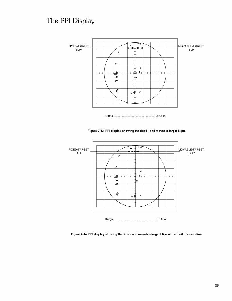
� 17. Slightly vary the orientation of each target so that the two target blips on thePPI display are of the same size.
On the Analog MTI Processor, set the GAIN control so that the two targetblips on the PPI display are as small as possible. Figure 2-43 shows anexample of what you might observed on the PPI display.
On the Target Controller, use the X-axis POSITION control to approach themovable target towards the fixed target, a few centimeters at a time, untilthe two target blips on the PPI display are as close as possible withoutmerging into one blip. Each time you move the movable target, readjust itsorientation so that its blip on the PPI display remains approximately thesame size. Figure 2-44 shows an example of what you might observe onthe PPI display.
� 18. On the PPI Scan Converter, use the EBL controls to determine thebearings of the fixed and movable targets. Note the results, then calculatethe difference between the bearings of the two targets. The result is theangle, with respect to the Radar Antenna, which separates the two targets.
�!������"�����
25
Range ........................................................: 3.6 m
MOVABLE-TARGETBLIP
FIXED-TARGETBLIP
Range ........................................................: 3.6 m
MOVABLE-TARGETBLIP
FIXED-TARGETBLIP
Figure 2-43. PPI display showing the fixed- and movable-target blips.
Figure 2-44. PPI display showing the fixed- and movable-target blips at the limit of resolution.

�!������"�����
26
Y
X
˜ 2.0 m
Compare this to the angular resolution that one would expect, knowing thatthe 3-dB beamwidth of the Radar Antenna is approximately 6�.
Range resolution of the pulsed radar
� 19. Remove the fixed mast from the target table.
Loosen the screw on the mast of the target table and turn the targetclockwise by approximately 90� so that it is parallel to the metal railsupporting the movable carriage. Tighten the screw in order to secure thetarget to the mast.
On the Target Controller, use the X- and Y-axis POSITION controls toplace the target at the following coordinates: X = 45 cm and Y = 45 cm.
Rotate the target table by 90� so that its position is as shown inFigure 2-45. Make sure that the grid is approximately 2.0 m from the hornof the Radar Antenna when the latter points towards the target, and that thetarget is correctly aligned with the shaft of the Rotating-Antenna Pedestal.
Note: Since the target table has been rotated by 90�, the X-axiscoordinates now correspond to the target range
Figure 2-45. Position of the target table.
�!������"�����
27
Range ........................................................: 3.6 m
METAL-TARGETBLIPPLEXIGLASS-TARGET
BLIP
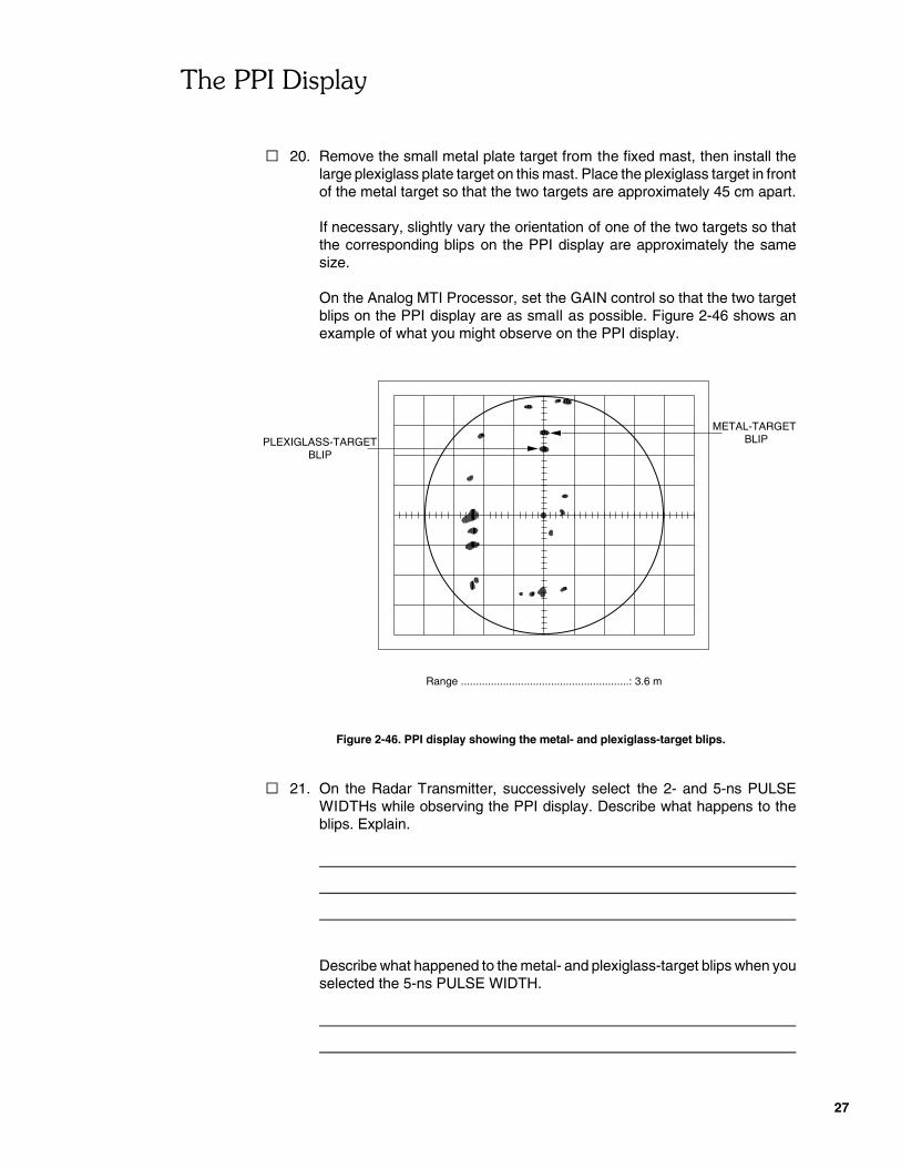
� 20. Remove the small metal plate target from the fixed mast, then install thelarge plexiglass plate target on this mast. Place the plexiglass target in frontof the metal target so that the two targets are approximately 45 cm apart.
If necessary, slightly vary the orientation of one of the two targets so thatthe corresponding blips on the PPI display are approximately the samesize.
On the Analog MTI Processor, set the GAIN control so that the two targetblips on the PPI display are as small as possible. Figure 2-46 shows anexample of what you might observe on the PPI display.
Figure 2-46. PPI display showing the metal- and plexiglass-target blips.
� 21. On the Radar Transmitter, successively select the 2- and 5-ns PULSEWIDTHs while observing the PPI display. Describe what happens to theblips. Explain.
Describe what happened to the metal- and plexiglass-target blips when youselected the 5-ns PULSE WIDTH.
�!������"�����
28
Range ........................................................: 3.6 m
METAL-TARGETBLIP
PLEXIGLASS-TARGETBLIP
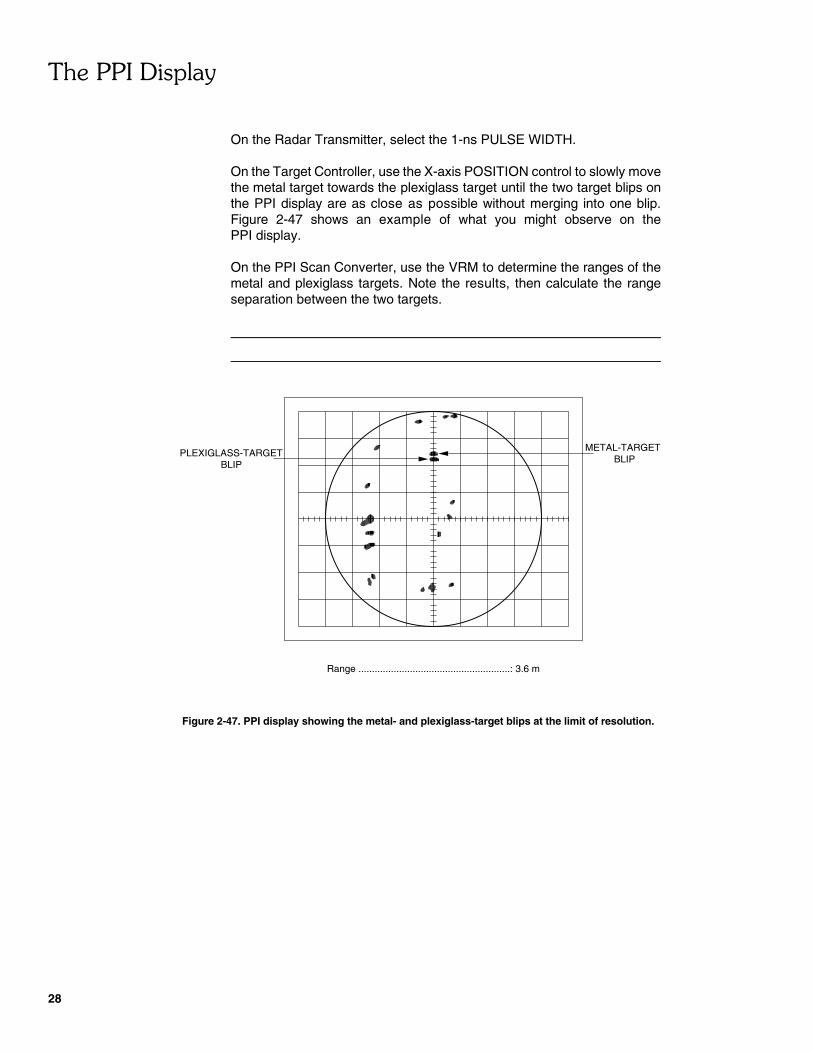
On the Radar Transmitter, select the 1-ns PULSE WIDTH.
On the Target Controller, use the X-axis POSITION control to slowly movethe metal target towards the plexiglass target until the two target blips onthe PPI display are as close as possible without merging into one blip.Figure 2-47 shows an example of what you might observe on thePPI display.
On the PPI Scan Converter, use the VRM to determine the ranges of themetal and plexiglass targets. Note the results, then calculate the rangeseparation between the two targets.
Figure 2-47. PPI display showing the metal- and plexiglass-target blips at the limit of resolution.

�!������"�����
29
Compare this range separation to the theoretical range resolution.
� 22. On the Radar Transmitter, make sure that the RF POWER switch is in theSTANDBY position. The RF POWER STANDBY LED should be lit. Placeall POWER switches in the O (off) position and disconnect all cables andaccessories.
CONCLUSION
In this exercise, you learned how to calibrate the origin of the PPI display, using atarget located at a known range and the VRM.
You learned the operation and use of various markers. You found that the VRM andthe range rings are used to determine the ranges of targets visible on thePPI display, whereas the EBL is used to determine the bearings of the targetsvisible on the PPI display.
You verified that the angular resolution of the pulsed radar is within 1 to 1.5 timesthe beamwidth of the Radar Antenna.
You established that, in practice, the range resolution of the pulsed radar issomewhat greater than one half the pulse length.
REVIEW QUESTIONS
1. What is meant by the term bearing?

�!������"�����
30
2. How are the range and bearing of each target represented on the PPI display?
3. Name and explain the use of one type of fixed markers on the PPI display.
4. Name and explain the use of two variable markers on the PPI display.
5. How does the gain of the radar receiver section affect the resolution of the PPIdisplay?

���������������
����
#���$�%�����������$

33
�����������
������������
EXERCISE OBJECTIVE
When you have completed this exercise, you will be familiar with blind speeds inMTI radar, and with range ambiguities which result in second-trace clutter. You willalso be familiar with the effect of staggered PRF on these two phenomena.
DISCUSSION
Blind speeds
In a vector-processing MTI radar, the output of the magnitude detector, as shownin equation (11) of Exercise 1-2, is
(1)
Magnitude � I 2� Q 2
� ��������
2A sin �fd
fp
where I and Q are the I- and Q-channel delay-line canceller output signalsrespectively,
A is the amplitude of the received echo signal,fd is the Doppler frequency of the received echo signal,fp is the pulse-repetition frequency (PRF).
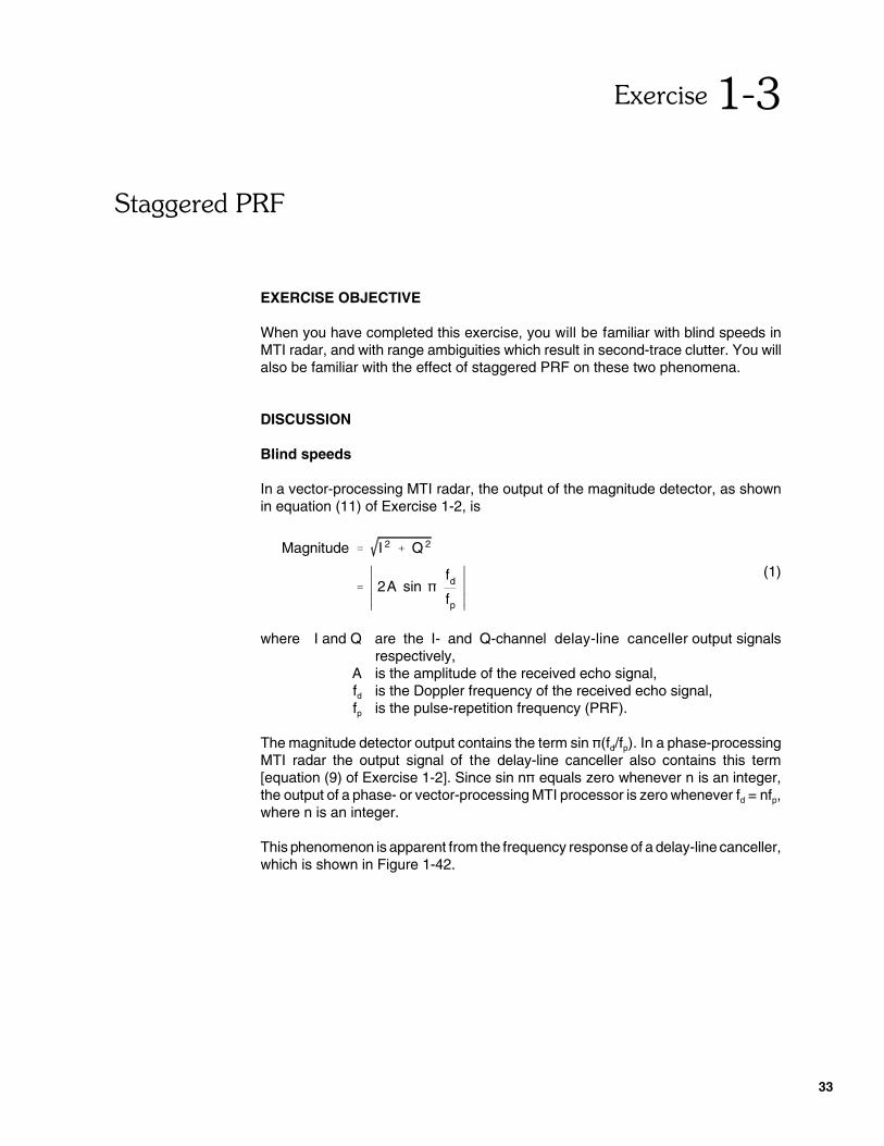
The magnitude detector output contains the term sin �(fd/fp). In a phase-processingMTI radar the output signal of the delay-line canceller also contains this term[equation (9) of Exercise 1-2]. Since sin n� equals zero whenever n is an integer,the output of a phase- or vector-processing MTI processor is zero whenever fd = nfp,where n is an integer.
This phenomenon is apparent from the frequency response of a delay-line canceller,which is shown in Figure 1-42.
���$$�������&
34
0
AM
PLI
TU
DE
FREQUENCY
fp p2f p3f p4f0
2
Figure 1-42. Frequency response of a delay-line canceler.
Nulls in the response of the canceller occur at multiples of the pulse-repetitionfrequency fp. If the Doppler frequency is a multiple of the pulse-repetition frequency,all of the frequency components of the canceller input signal will lie in the nulls.When this happens, the signal is rejected and the output of the canceller is zero.
Because of this phenomenon, moving targets with certain radial velocities produceno output from the MTI processor. These radial velocities are known as blindspeeds, since the MTI radar does not "see" these targets.
From equation (9) of Exercise 1-1, the Doppler frequency of a moving target isequal to
(2)fd �
2ft
cv cos � �
2ft
cvrad
where fd is the Doppler frequency, in Hz,ft is the transmitted frequency,c is the speed of light (3.00 x 10⁸ m/s),v is the target speed,� is the angle between the target direction and the line of sight,
vrad is the radial velocity, or range rate.
A blind speed occurs when
(3)fd
fp
�
2ft
cfp
vrad � n, n an integer.
Therefore, blind speeds occur at the radial velocities
vn �
ncfp
2ft
� n3 × 108 × fp (Hz)
2 × ft (Hz)(m/s)
� n0.15 × fp (Hz)
ft (GHz)(m/s) for n � 1, 2, 3 ...
���$$�������&
35
where vn is the nth blind speed,c is the speed of light,fp is the pulse-repetition frequency (PRF),ft is the transmitted frequency.
For example, if the transmitted frequency ft is 2 GHz and the PRF is 600 Hz, thefirst blind speed is
v1 �0.15 × 600 Hz
2 GHz� 45 m/s � 162 km/h
Blind speeds are one of the limitations of MTI radar. They exist in pulsed radarbecause the radar signal, and therefore the phase detector output signal, are pulsedrather than continuous.
Blind speeds would not be a problem if the first blind speed were always greaterthan the maximum radial velocity expected of a target. For this, the ratio fp/ft wouldhave to be large, that is, the pulse-repetition frequency high and the transmittedfrequency low. Unfortunately, there are other constraints on these parameters whichoften make it difficult to avoid blind speeds. Low transmit frequencies have thedisadvantage that they result in a large antenna beamwidth and therefore poorangular resolution of the radar. High pulse-repetition frequencies are oftenimpractical because they can cause the range measurements to be ambiguous.
Range ambiguity
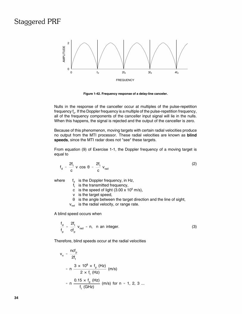
During the time interval between transmitted radar pulses, the radar "listens" forechoes. This is illustrated in Figure 1-43. In (a), one echo is received during eachpulse-repetition interval T. The round-trip transit time TR is quite long, showing thatthe target is relatively far from the radar.
���$$�������&
36
TIMEPULSEECHO
2 3PULSE
1ECHO
21PULSE
TRANSIT TIME TR
PULSE-REPETITIONINTERVAL T
T= 1/f p
A) UNAMBIGUOUS RANGE
1PULSE PULSE
1ECHO
2
PULSE-REPETITION
T= 1/f
TRANSIT TIME TR
p
INTERVAL T
PULSE ECHO34
TIME
B) AMBIGUOUS RANGE
3 2ECHOPULSE
ACTUAL
T − TAPPARENT TRANSIT TIME
R
SECOND-TRACEECHO
Figure 1-43. Second-trace echoes.
However, since the pulse-repetition interval is greater than the transit time, eachtransmitted pulse has time to reach the target and return as an echo before the nextpulse is transmitted.
Figure 1-43 (b) shows the effect of increasing the pulse-repetition frequency fp untilthe pulse-repetition interval is less than the transit time. Now, a second pulse istransmitted before the first echo has time to return to the radar. The first echoarrives shortly after transmission of the second pulse. Since there is no way oftelling which echo results from which pulse, the round-trip transit time "perceived"by the radar is much less that the actual transit time. The target, therefore, appearsat a much closer range than its actual range. This phenomenon makes the rangemeasurement ambiguous.
An echo which is received after a time delay exceeding one pulse-repetition interval,but less than two pulse-repetition intervals, is called a second-trace echo or a
���$$�������&
37
second-time-around echo. Third-trace (third-time-around) echoes are defined ina similar manner. The terms multiple-trace echoes and multiple-time-around echoesare sometimes used.
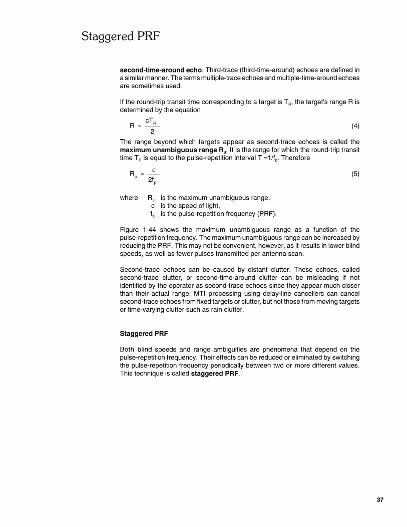
If the round-trip transit time corresponding to a target is TR, the target's range R isdetermined by the equation
(4)R �
cTR
2
The range beyond which targets appear as second-trace echoes is called themaximum unambiguous range Ru. It is the range for which the round-trip transittime TR is equal to the pulse-repetition interval T =1/fp. Therefore
(5)Ru �c
2fp
where Ru is the maximum unambiguous range,c is the speed of light,fp is the pulse-repetition frequency (PRF).
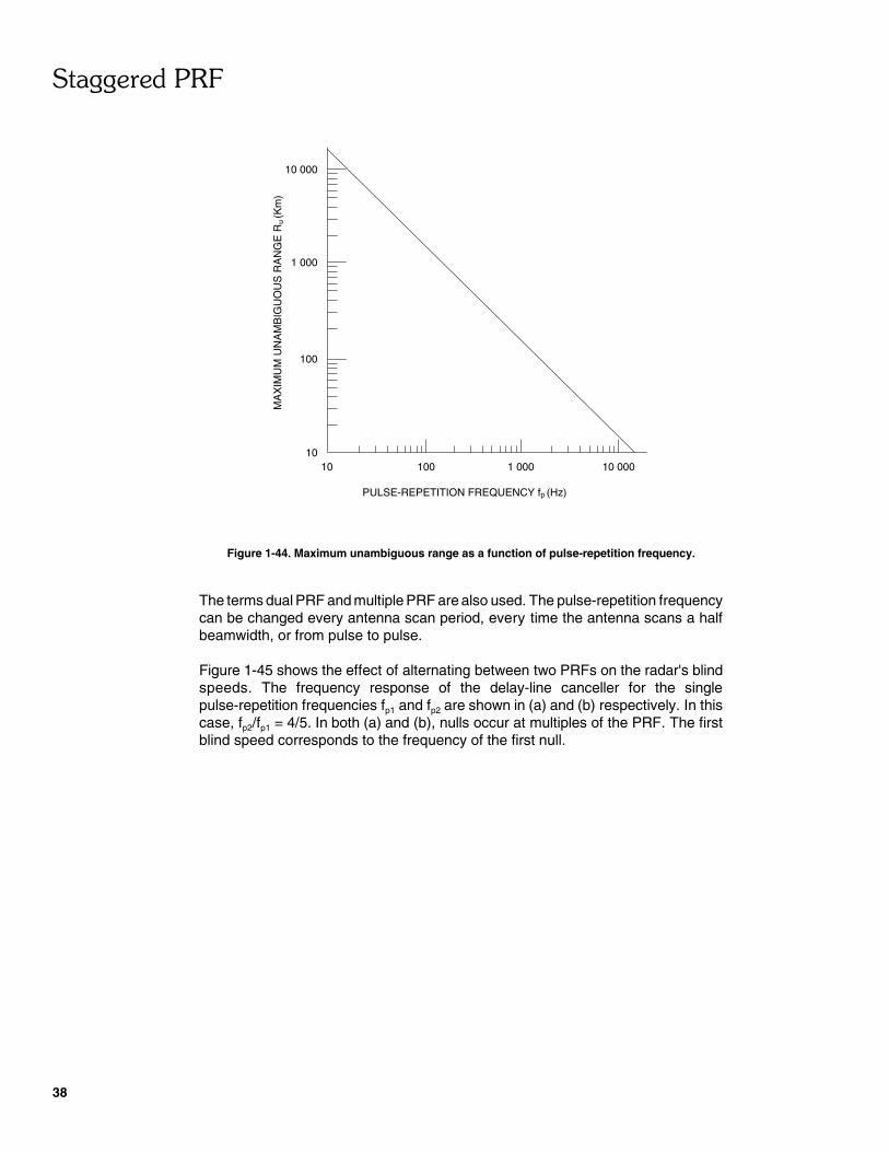
Figure 1-44 shows the maximum unambiguous range as a function of thepulse-repetition frequency. The maximum unambiguous range can be increased byreducing the PRF. This may not be convenient, however, as it results in lower blindspeeds, as well as fewer pulses transmitted per antenna scan.
Second-trace echoes can be caused by distant clutter. These echoes, calledsecond-trace clutter, or second-time-around clutter can be misleading if notidentified by the operator as second-trace echoes since they appear much closerthan their actual range. MTI processing using delay-line cancellers can cancelsecond-trace echoes from fixed targets or clutter, but not those from moving targetsor time-varying clutter such as rain clutter.
Staggered PRF
Both blind speeds and range ambiguities are phenomena that depend on thepulse-repetition frequency. Their effects can be reduced or eliminated by switchingthe pulse-repetition frequency periodically between two or more different values.This technique is called staggered PRF.
���$$�������&
38
MA
XIM
UM
UN
AM
BIG
UO
US
RA
NG
E R
(K
m)
PULSE-REPETITION FREQUENCY f (Hz)
10 100 1 000 10 00010
100
1 000
10 000
u
p
Figure 1-44. Maximum unambiguous range as a function of pulse-repetition frequency.
The terms dual PRF and multiple PRF are also used. The pulse-repetition frequencycan be changed every antenna scan period, every time the antenna scans a halfbeamwidth, or from pulse to pulse.
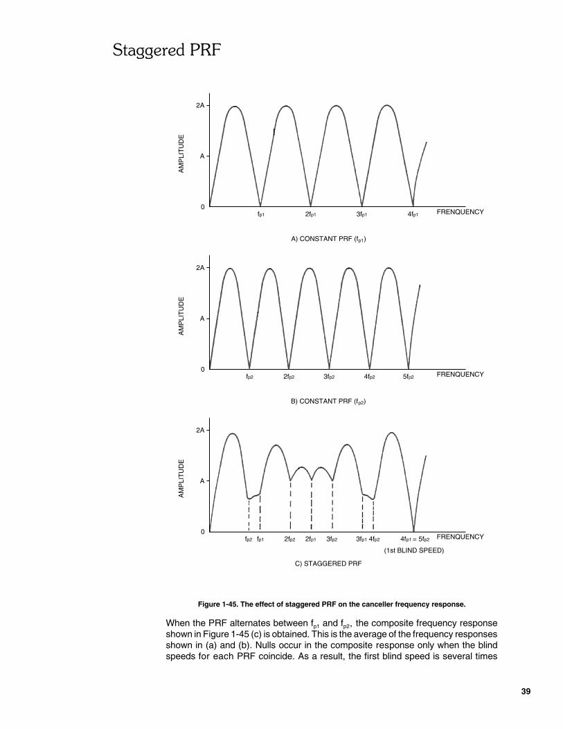
Figure 1-45 shows the effect of alternating between two PRFs on the radar's blindspeeds. The frequency response of the delay-line canceller for the singlepulse-repetition frequencies fp1 and fp2 are shown in (a) and (b) respectively. In thiscase, fp2/fp1 = 4/5. In both (a) and (b), nulls occur at multiples of the PRF. The firstblind speed corresponds to the frequency of the first null.
���$$�������&
39
2A
A
0
AM
PLI
TU
DE
A) CONSTANT PRF (f )p1
p1f p12f p13f p14f FRENQUENCY
(1st BLIND SPEED)
AM
PLI
TU
DE
A
2A
0
B) CONSTANT PRF (f )
p2f p22fp2
p2
p23f 4f FRENQUENCY
AM
PLI
TU
DE
A
2A
0p1f p12f FRENQUENCY
C) STAGGERED PRF
3fp1 4fp1
p25f
fp2 2fp2 p23f p24f p2= 5f
Figure 1-45. The effect of staggered PRF on the canceller frequency response.
When the PRF alternates between fp1 and fp2, the composite frequency responseshown in Figure 1-45 (c) is obtained. This is the average of the frequency responsesshown in (a) and (b). Nulls occur in the composite response only when the blindspeeds for each PRF coincide. As a result, the first blind speed is several times
���$$�������&
40
1PULSE PULSE
1ECHO
2
PULSE-REPETITION
T = 1/f
TRANSIT TIME TR
p1
INTERVAL T
PULSE ECHO23
TIME
A) PULSE-REPETITION FREQUENCY = f
ACTUAL
T − TAPPARENT TRANSIT TIME
R1
1
1
RT − TAPPARENT TRANSIT TIME
p2
PULSE-REPETITIONINTERVAL T
ACTUALTRANSIT TIME T
PULSE1
T = 1/f2
B) PULSE-REPETITION FREQUENCY = f
PULSE2
2
R
ECHO1
ECHOPULSE3
2
2
TIME
p1
p2
greater than when one PRF is used. In this example, the first blind speedcorresponds to 4fp1 = 5fp2.
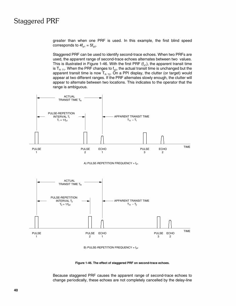
Staggered PRF can be used to identify second-trace echoes. When two PRFs areused, the apparent range of second-trace echoes alternates between two values.This is illustrated in Figure 1-46. With the first PRF (fp1), the apparent transit timeis TR�T1. When the PRF changes to fp2, the actual transit time is unchanged but theapparent transit time is now TR�T2. On a PPI display, the clutter (or target) wouldappear at two different ranges. If the PRF alternates slowly enough, the clutter willappear to alternate between two locations. This indicates to the operator that therange is ambiguous.
Figure 1-46. The effect of staggered PRF on second-trace echoes.
Because staggered PRF causes the apparent range of second-trace echoes tochange periodically, these echoes are not completely cancelled by the delay-line
���$$�������&
41
canceller. If the PRF is changed from pulse to pulse, they are not cancelled at all.This is one disadvantage of the staggered-PRF technique. In some systems, aconstant PRF is used over those angular sectors where second-trace clutter isexpected and staggered PRF is used elsewhere.
Note: A frequency counter with at least a 1-Hz resolution (Lab-VoltModel 9403 or equivalent) must be used.
Procedure Summary
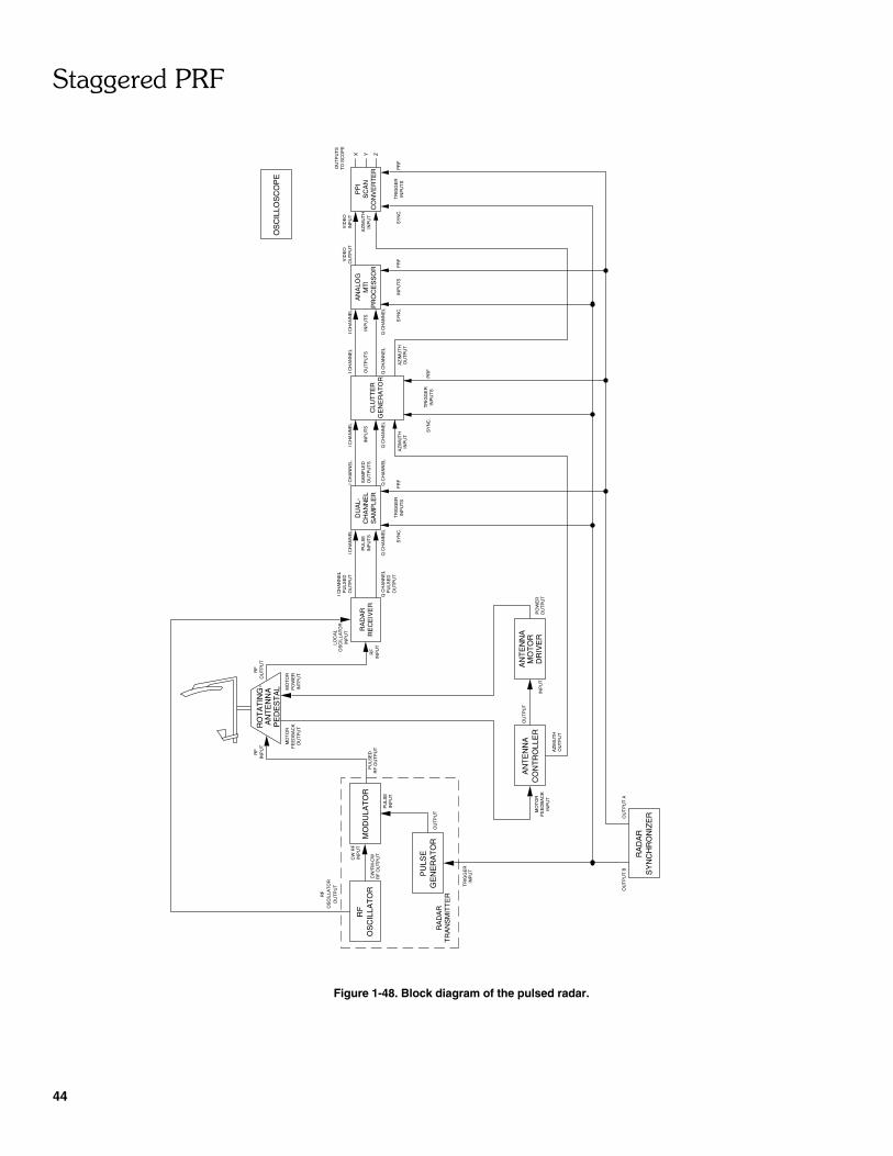
The first part of this exercise is Setting up the pulsed radar. The block diagram ofthe system you will use is shown in Figure 1-48. The connection of the oscilloscopeis not shown in this figure since you will use it to first adjust the signal levels andthen the dc offset voltages, at the SAMPLED OUTPUTS of the Dual-ChannelSampler.
In the second part of this exercise, The blind speeds phenomenon, you will observe,in the time domain, the echo from a moving target at various points within thereceiver of a vector-processing MTI radar. A frequency counter will be used tomeasure the Doppler frequency fd related to the radial velocity of the moving target.This will allow you to observe the blind speeds phenomenon, to explain itsundesired effect on receiver sensitivity, and to understand how blind speeds occur.
In the third part of this exercise, Staggered PRF, you will observe, in the timedomain, the PRF signal in the 288-Hz staggered-PRF mode. This will allow you todetermine on which basis the PRF is switched, to measure the interpulse periodsrelated to the PRFs used in this mode, and to calculate the PRF ratio. You will thenused this ratio to predict the frequency at which the first blind speed should occurin this mode.
In the fourth part of this exercise, Frequency response of the MTI circuit instaggered PRF, you will inject a sine-wave signal of known amplitude into theI-channel MTI circuit (single delay-line canceller) and observe the resulting signalat its output in the 288-Hz staggered-PRF mode. You will then vary the frequencyof the sine-wave signal and measure the amplitude of the signal at the output of theMTI circuit. The results of the measurements will be used to plot thefrequency-response curve of the MTI circuit in the 288-Hz staggered-PRF mode.
In the fifth part of this exercise, Effect of staggered PRF on blind speeds, you willcomplete the connections and settings required to obtain the PPI display. You willthen observe the blind speeds phenomenon on the PPI display and the effectstaggered PRF has on blind speeds.
The observations and measurements made in the previous parts of this exercise willbe useful to explain what happens on the PPI display.
In the sixth part of this exercise, Effect of staggered PRF on second trace echoes,you will use the Clutter Generator to produce a second trace echo on thePPI display. You will then observe the second trace echo on the PPI display for twodifferent single PRFs in order to see and explain what happens when the PRF is
���$$�������&
42
changed. You will finally observe the effect staggered PRF has on the second traceecho on the PPI display.
Note: This exercise is quite long. However, the PROCEDURE containsinstructions, enclosed in rectangles, that allow the exercise to bedivided in two parts and carried out in two separate laboratory periodsas described below.
In the first laboratory period, the following PROCEDURE subsectionscan be carried out:– Setting up the pulsed radar,– The blind speeds phenomenon,– Staggered PRF,– Frequency response of the MTI circuit in staggered PRF.In the second laboratory period, the following PROCEDUREsubsections can be carried out:– Setting up the pulsed radar,– Effect of staggered PRF on blind speeds,– Effect of staggered PRF on second trace echoes.
PROCEDURE
Setting up the pulsed radar
� 1. The main elements of the Radar Training System, that is the antenna andits pedestal, the target table and the training modules, must be set upproperly before beginning this exercise. Refer to Appendix A of this manualfor setting up the Radar Training System, if this has not already been done.
Set up the modules on the Power Supply / Antenna Motor Driver as shownin Figure 1-47.
On the Radar Transmitter, make sure that the RF POWER switch is in theSTANDBY position.
On the Antenna Controller, make sure that the MANual ANTENNAROTATION MODE push button is depressed and that the SPEED controlis in the O position.
Set the POWER switch of the Power Supply to the I (on) position. Do thesame for the other modules that have a POWER switch.
� 2. Figure 1-48 shows the block diagram of the pulsed radar, including thePPI display, that can be obtained with the Radar Training System.
���$$�������&
43
RADAR TRANSMITTER
RADAR RECEIVERCLUTTER GENERATOR
DUAL-CHANNEL SAMPLER
ANTENNA MOTOR DRIVERPOWER SUPPLYOSCILLOSCOPE
ANALOGMTI PROCESSOR
SCAN CONVERTERPPI
RADAR SYNCHRONIZER/ANTENNA CONTROLLER
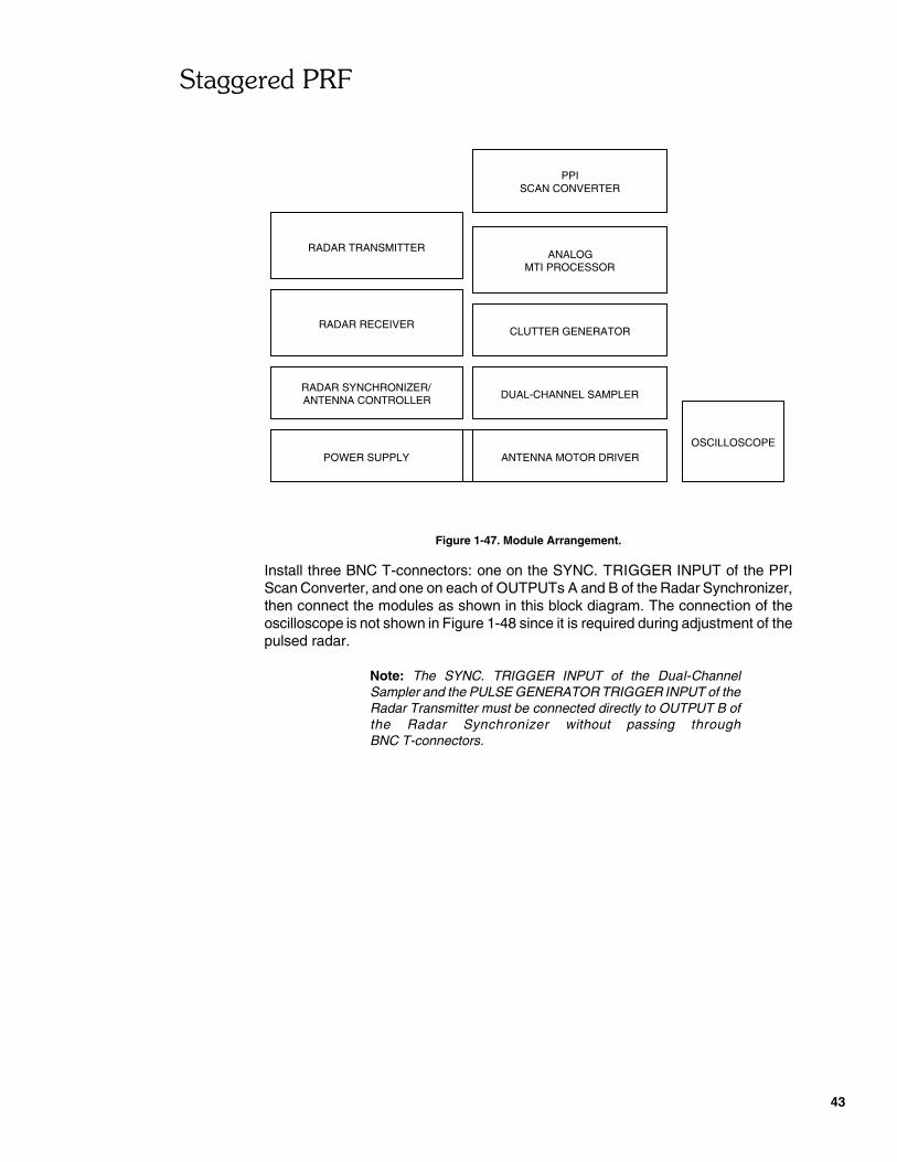
Figure 1-47. Module Arrangement.
Install three BNC T-connectors: one on the SYNC. TRIGGER INPUT of the PPIScan Converter, and one on each of OUTPUTs A and B of the Radar Synchronizer,then connect the modules as shown in this block diagram. The connection of theoscilloscope is not shown in Figure 1-48 since it is required during adjustment of thepulsed radar.
Note: The SYNC. TRIGGER INPUT of the Dual-ChannelSampler and the PULSE GENERATOR TRIGGER INPUT of theRadar Transmitter must be connected directly to OUTPUT B ofthe Radar Synchronizer without passing throughBNC T-connectors.
���$$�������&
44
INP
UT
PO
WE
RM
OT
OR
INT
PU
T
RO
TA
TIN
G-
PE
DE
ST
AL
AN
TE
NN
AO
UT
PU
T
OU
TP
UT
B SY
NC
HR
ON
IZE
RR
AD
AR
OU
TP
UT
A
MO
TO
R
INP
UT
FE
ED
BA
CK
AZ
IMU
TH
OU
TP
UT
CO
NT
RO
LLE
R
INP
UT
TR
IGG
ER
OS
CIL
LAT
OR
GE
NE
RA
TO
R
TR
AN
SM
ITT
ER
RA
DA
R
OS
CIL
LAT
OR
RF
OU
TP
UT
RF
PU
LSE
OU
TP
UT
MO
DU
LAT
OR
CW
/FM
-CW
RF
OU
TP
UT
CW
RF
INP
UT
PU
LSE
INP
UT
PU
LSE
DR
F O
UT
PU
TFE
ED
BA
CK
MO
TO
R
OU
TP
UT
INP
UT
RF
AN
TE
NN
A
MO
TO
RD
RIV
ER
PO
WE
RO
UT
PU
T
CO
NV
ER
TE
RS
CA
N
INP
UT
ST
RIG
GE
R
OS
CIL
LOS
CO
PE
INP
UT
S
AN
TE
NN
A
Q C
HA
NN
EL
PU
LSE
DO
UT
PU
T
I CH
AN
NE
LP
ULS
ED
OU
TP
UT
OS
CIL
LAT
OR
INP
UT
RF
INP
UT
RE
CE
IVE
RR
AD
AR
LOC
AL
I CH
AN
NE
L
Q C
HA
NN
EL
SY
NC
.
PU
LSE
INP
UT
S
TR
IGG
ER
SA
MP
LER
DU
AL-
CH
AN
NE
LA
NA
LOG
PR
OC
ES
SO
R
INP
UT
S
Q C
HA
NN
EL
I CH
AN
NE
L
INP
UT
S
Q C
HA
NN
EL
PR
FI CH
AN
NE
L
OU
TP
UT
SS
AM
PLE
D
SY
NC
.
MT
IA
ZIM
UT
H
PR
FVID
EO
OU
TP
UT
SY
NC
.
INP
UT
INP
UT
VID
EO
PP
I
OU
TP
UT
RF
PR
F
Z
TO
SC
OP
E
X Y
OU
TP
UT
S
GE
NE
RA
TO
RC
LUT
TE
R
I CH
AN
NE
L
Q C
HA
NN
EL
INP
UT
S
I CH
AN
NE
L
OU
TP
UT
S
Q C
HA
NN
EL
SY
NC
.T
RIG
GE
RIN
PU
TS
PR
F
AZ
IMU
TH
OU
TP
UT
AZ
IMU
TH
INP
UT
Figure 1-48. Block diagram of the pulsed radar.

���$$�������&
45
� 3. Make the following adjustments:
On the Radar Transmitter
RF OSCILLATOR FREQUENCY . . . . . . . CAL.PULSE GENERATOR PULSE WIDTH . . 1 ns
On the Radar Synchronizer
PRF MODE . . . . . . . . . . . . . . . . . . . . SINGLEPRF . . . . . . . . . . . . . . . . . . . . . . . . . . . 288 Hz
On the Dual-Channel Sampler
RANGE SPAN . . . . . . . . . . . . . . . . . . . . 3.6 m
On the Analog MTI Processor
RANGE . . . . . . . . . . . . . . . . . . . . . . . . . . . . . : 3.6 m
On the Clutter Generator
SEA CLUTTER . . . . . . . . . . . . . . . . . . . . . . . : OFFRAIN CLUTTER / SECOND-TRACE-ECHO . . . . . . . . . . . . . . . : OFF
POSITION R . . . . . . . . . . . . . . . . . . . . . . . : MIN.POSITION � . . . . . . . . . . . . . . . . . . . . . . . : 0�AREA �R . . . . . . . . . . . . . . . . . . . . . . . . . : MIN.AREA �� . . . . . . . . . . . . . . . . . . . . . . . . . . : MIN.
INTERFERENCE / NOISE . . . . . . . . . . . . . . : OFF
� 4. Connect the cable of the target table to the multi-pin connector located onthe rear panel of the Target Controller. Make sure that the surface of thetarget table is free of any objects and then set the POWER switch of theTarget Positioning System to the I (on) position.
Place the target table so that its grid is located approximately 1.5 m fromthe Rotating-Antenna Pedestal, as shown in Figure 1-49. Make sure thatthe metal rail of the target table is correctly aligned with the shaft of theRotating-Antenna Pedestal.
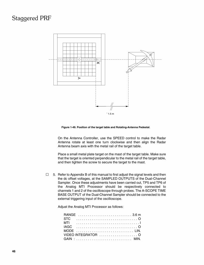
���$$�������&
46
˜ 1.5 m
Y
X
Figure 1-49. Position of the target table and Rotating-Antenna Pedestal.
On the Antenna Controller, use the SPEED control to make the RadarAntenna rotate at least one turn clockwise and then align the RadarAntenna beam axis with the metal rail of the target table.
Place a small metal plate target on the mast of the target table. Make surethat the target is oriented perpendicular to the metal rail of the target table,and then tighten the screw to secure the target to the mast.
� 5. Refer to Appendix B of this manual to first adjust the signal levels and thenthe dc offset voltages, at the SAMPLED OUTPUTS of the Dual-ChannelSampler. Once these adjustments have been carried out, TP5 and TP6 ofthe Analog MTI Processor should be respectively connected tochannels 1 and 2 of the oscilloscope through probes. The A-SCOPE TIMEBASE OUTPUT of the Dual-Channel Sampler should be connected to theexternal triggering input of the oscilloscope.
Adjust the Analog MTI Processor as follows:
RANGE . . . . . . . . . . . . . . . . . . . . . . . . . . . . 3.6 mSTC . . . . . . . . . . . . . . . . . . . . . . . . . . . . . . . . OMTI . . . . . . . . . . . . . . . . . . . . . . . . . . . . . . . . . IIAGC . . . . . . . . . . . . . . . . . . . . . . . . . . . . . . . . OMODE . . . . . . . . . . . . . . . . . . . . . . . . . . . . . . LIN.VIDEO INTEGRATOR . . . . . . . . . . . . . . . . . . . . OGAIN : . . . . . . . . . . . . . . . . . . . . . . . . . . . . . MIN.
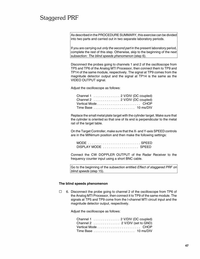
���$$�������&
47
As described in the PROCEDURE SUMMARY, this exercise can be dividedinto two parts and carried out in two separate laboratory periods.
If you are carrying out only the second part in the present laboratory period,complete the rest of this step. Otherwise, skip to the beginning of the nextsubsection: The blind speeds phenomenon (step 6).
Disconnect the probes going to channels 1 and 2 of the oscilloscope fromTP5 and TP6 of the Analog MTI Processor, then connect them to TP9 andTP14 of the same module, respectively. The signal at TP9 comes from themagnitude detector output and the signal at TP14 is the same as theVIDEO OUTPUT signal.
Adjust the oscilloscope as follows:
Channel 1 . . . . . . . . . . . . . . 2 V/DIV (DC coupled)Channel 2 . . . . . . . . . . . . . . 2 V/DIV (DC coupled)Vertical Mode . . . . . . . . . . . . . . . . . . . . . . . CHOPTime Base . . . . . . . . . . . . . . . . . . . . . . 10 ms/DIV
Replace the small metal plate target with the cylinder target. Make sure thatthe cylinder is oriented so that one of its end is perpendicular to the metalrail of the target table.
On the Target Controller, make sure that the X- and Y-axis SPEED controlsare in the MINimum position and then make the following settings:
MODE . . . . . . . . . . . . . . . . . . . . . . . . . . . . SPEEDDISPLAY MODE . . . . . . . . . . . . . . . . . . . SPEED
Connect the CW DOPPLER OUTPUT of the Radar Receiver to thefrequency counter input using a short BNC cable.
Go to the beginning of the subsection entitled Effect of staggered PRF onblind speeds (step 15).
The blind speeds phenomenon
� 6. Disconnect the probe going to channel 2 of the oscilloscope from TP6 ofthe Analog MTI Processor, then connect it to TP9 of the same module. Thesignals at TP5 and TP9 come from the I-channel MTI circuit input and themagnitude detector output, respectively.
Adjust the oscilloscope as follows:
Channel 1 . . . . . . . . . . . . . . 2 V/DIV (DC coupled)Channel 2 . . . . . . . . . . . . . . 2 V/DIV (set to GND)Vertical Mode . . . . . . . . . . . . . . . . . . . . . . . CHOPTime Base . . . . . . . . . . . . . . . . . . . . . . 10 ms/DIV
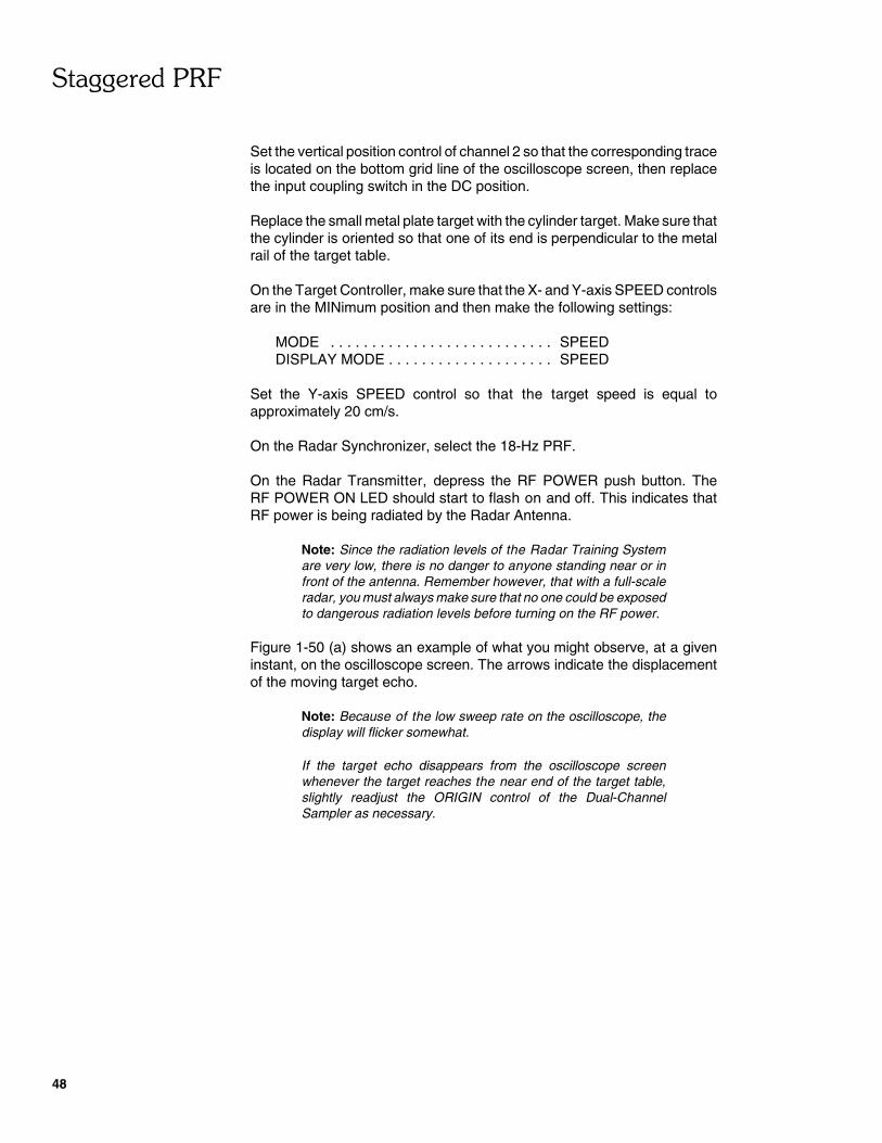
���$$�������&
48
Set the vertical position control of channel 2 so that the corresponding traceis located on the bottom grid line of the oscilloscope screen, then replacethe input coupling switch in the DC position.
Replace the small metal plate target with the cylinder target. Make sure thatthe cylinder is oriented so that one of its end is perpendicular to the metalrail of the target table.
On the Target Controller, make sure that the X- and Y-axis SPEED controlsare in the MINimum position and then make the following settings:
MODE . . . . . . . . . . . . . . . . . . . . . . . . . . . SPEEDDISPLAY MODE . . . . . . . . . . . . . . . . . . . . SPEED
Set the Y-axis SPEED control so that the target speed is equal toapproximately 20 cm/s.
On the Radar Synchronizer, select the 18-Hz PRF.
On the Radar Transmitter, depress the RF POWER push button. TheRF POWER ON LED should start to flash on and off. This indicates thatRF power is being radiated by the Radar Antenna.
Note: Since the radiation levels of the Radar Training Systemare very low, there is no danger to anyone standing near or infront of the antenna. Remember however, that with a full-scaleradar, you must always make sure that no one could be exposedto dangerous radiation levels before turning on the RF power.
Figure 1-50 (a) shows an example of what you might observe, at a giveninstant, on the oscilloscope screen. The arrows indicate the displacementof the moving target echo.
Note: Because of the low sweep rate on the oscilloscope, thedisplay will flicker somewhat.
If the target echo disappears from the oscilloscope screenwhenever the target reaches the near end of the target table,slightly readjust the ORIGIN control of the Dual-ChannelSampler as necessary.
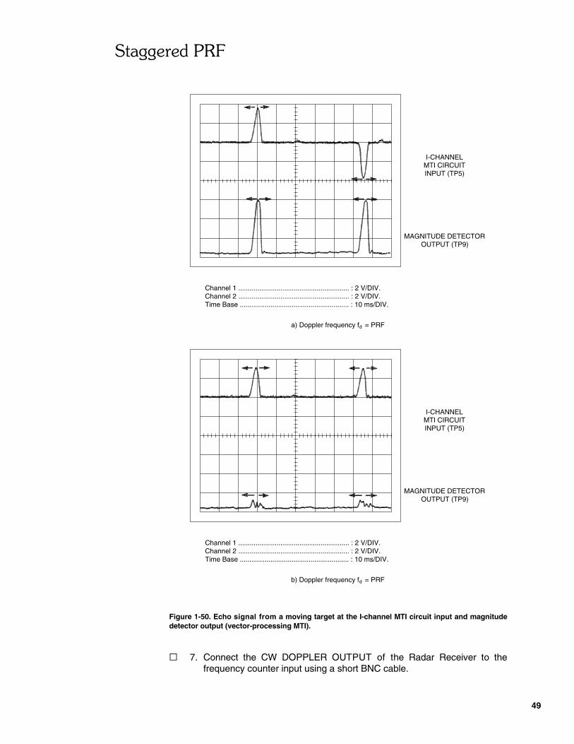
���$$�������&
49
Time Base ......................................................... : 10 ms/DIV.Channel 2 .......................................................... : 2 V/DIV.Channel 1 .......................................................... : 2 V/DIV.
MAGNITUDE DETECTOR
MTI CIRCUITI-CHANNEL
INPUT (TP5)
OUTPUT (TP9)
a) Doppler frequency f = PRFd
MAGNITUDE DETECTOROUTPUT (TP9)
INPUT (TP5)MTI CIRCUITI-CHANNEL
Channel 1 .......................................................... : 2 V/DIV.Channel 2 .......................................................... : 2 V/DIV.Time Base ......................................................... : 10 ms/DIV.
b) Doppler frequency f = PRFd
Figure 1-50. Echo signal from a moving target at the I-channel MTI circuit input and magnitudedetector output (vector-processing MTI).
� 7. Connect the CW DOPPLER OUTPUT of the Radar Receiver to thefrequency counter input using a short BNC cable.

���$$�������&
50
The frequency counter indicates the frequency at which the amplitude ofthe target echo varies, that is, the Doppler frequency fd related to themoving target speed, which in this case, is equal to the radial velocity.
Note: Since the target goes back and forth over the target table,the reading on the frequency counter fluctuates whenever thetarget reaches either end of the target table.
Read the Doppler frequency fd on the frequency counter and write the resultbelow.
Doppler frequency fd = _______Hz
Are the conditions required for a blind speed to occur met? Explain.
� 8. On the Target Controller, use the Y-axis SPEED control to slowly increasethe target speed, while observing the oscilloscope screen, until thefrequency counter indicates 18 Hz most of the time. Figure 1-50 (b) showsan example of what you might observe, at a given instant, on theoscilloscope screen. The arrows indicate the displacement of the movingtarget echo.
Describe what happens to the target echo at the magnitude detector outputas the target speed is increased until the Doppler frequency fd is equal to18 Hz. Explain why.
Calculate the first blind speed v1 related to the MTI radar presently used.
The Y-axis SPEED DISPLAY of the Target Controller indicates the radialvelocity vrad of the moving target.
Measure the radial velocity vrad of the moving target.
Radial velocity vrad = _______ cm/s

���$$�������&
51
MTI CIRCUIT
OUTPUT (TP7)
I-CHANNELMTI CIRCUIT
Q-CHANNEL
Channel 1 .......................................................... : 2 V/DIV.Channel 2 .......................................................... : 2 V/DIV.Time Base ......................................................... : 10 ms/DIV.
OUTPUT (TP8)
Compare the radial velocity vrad of the moving target with the first blindspeed v1 calculated before. Is the equation for calculating blind speedsverified?
Describe the problem caused by blind speeds.
� 9. Disconnect the probes going to channels 1 and 2 of the oscilloscope fromTP5 and TP9 of the Analog MTI Processor, then connect them to TP7 andTP8 of the same module, respectively. The signals at TP7 and TP8presently come from the I- and Q-channel MTI circuit outputs.
On the oscilloscope, place the input coupling switch of channel 2 in theGND position. Set the vertical position control of channel 2 so that thecorresponding trace is centred in the lower half of the oscilloscope screen,then replace the input coupling switch in the DC position. Figure 1-51shows an example of what you might observe, at a given instant, on theoscilloscope screen. The arrows indicate the displacement of the movingtarget echo residue.
Figure 1-51. Echo signal of a moving target at the outputs of the I-and Q-channel MTI circuits (singledelay-line cancellers), in a blind speed situation.
���$$�������&
52
From this figure, explain how blind speeds occur in a phase- orvector-processing MTI radar. Explain why.
Staggered PRF
� 10. On the Radar Transmitter, place the RF POWER switch in the STANDBYposition.
On the Target Controller, set the Y-axis SPEED control to the MIN. positionto stop the target.
Remove the probes connected to the oscilloscope.
On the Dual-Channel Sampler, disconnect the cable connecting thePRF TRIGGER INPUT to OUTPUT A of the Radar Synchronizer, thenconnect it to channel 2 of the oscilloscope.
Make the following adjustments:
On the Radar Synchronizer
PRF . . . . . . . . . . . . . . . . . . . . . . . . . . . 288 HzPRF MODE . . . . . . . . . . . . . . . STAGGERED
On the oscilloscope
Vertical Mode . . . . . . . . . . . . . . . . . Channel 2Trigger . . . . . . . . . . . . . . . . . . . . . . Channel 2
The staggered-PRF signal on the oscilloscope screen is probably notstable. If this is the case, use the magnifying control to magnify thestaggered-PRF signal on the oscilloscope screen. Carefully and slowlyadjust the holdoff control until the signal is stable, then return to anon-magnified display. Figure 1-52 shows an example of what you mightobserve on the oscilloscope screen.
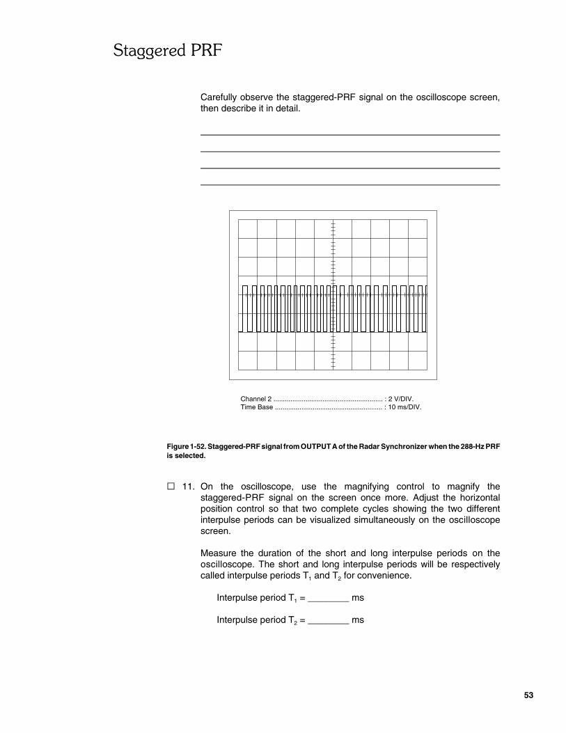
���$$�������&
53
Channel 2 .......................................................... : 2 V/DIV.Time Base ......................................................... : 10 ms/DIV.
Carefully observe the staggered-PRF signal on the oscilloscope screen,then describe it in detail.
Figure 1-52. Staggered-PRF signal from OUTPUT A of the Radar Synchronizer when the 288-Hz PRFis selected.
� 11. On the oscilloscope, use the magnifying control to magnify thestaggered-PRF signal on the screen once more. Adjust the horizontalposition control so that two complete cycles showing the two differentinterpulse periods can be visualized simultaneously on the oscilloscopescreen.
Measure the duration of the short and long interpulse periods on theoscilloscope. The short and long interpulse periods will be respectivelycalled interpulse periods T1 and T2 for convenience.
Interpulse period T1 = ________ ms
Interpulse period T2 = ________ ms

���$$�������&
54
Calculate the pulse-repetition frequencies corresponding to interpulseperiods T1 and T2, that is PRF1 and PRF2 respectively, then calculate thePRF ratio PRF1/PRF2.
From these results, calculate the Doppler frequency fd at which the firstblind speed should occur using the 288-Hz staggered PRF.
On the oscilloscope, return to a non-magnified display then set the holdoffcontrol to its normal position.
On the oscilloscope, disconnect the cable connected to the input ofchannel 2, then reconnect it to the PRF TRIGGER INPUT of the Dual-Channel Sampler.
Frequency response of the MTI circuit in staggered PRF
� 12. Using probes, connect TP5 and TP7 of the Analog MTI Processor tochannels 1 and 2 of the oscilloscope, respectively. The signals at TP5 andTP7 come from the input and output of the I-channel MTI circuit (singledelay-line canceller).
On the Analog MTI Processor, disconnect the cable connecting theI-CHANNEL INPUT to the I-CHANNEL OUTPUT of the Clutter Generator.
Set the controls of the function generator so that it produces a 200-Hzsine-wave signal having an amplitude of 100 mV, then connect its outputto the I-CHANNEL INPUT of the Analog MTI Processor.
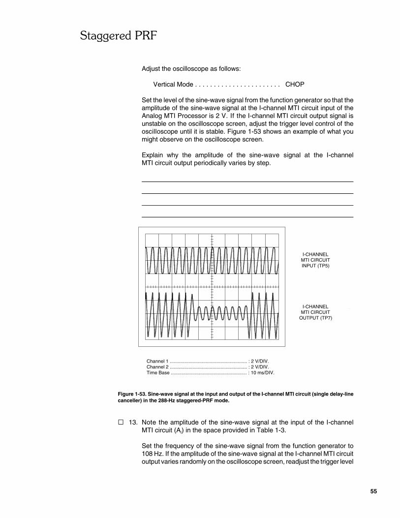
���$$�������&
55
INPUT (TP5)
I-CHANNELMTI CIRCUIT
Channel 1 .......................................................... : 2 V/DIV.Channel 2 .......................................................... : 2 V/DIV.Time Base ......................................................... : 10 ms/DIV.
MTI CIRCUITI-CHANNEL
OUTPUT (TP7)
Adjust the oscilloscope as follows:
Vertical Mode . . . . . . . . . . . . . . . . . . . . . . . CHOP
Set the level of the sine-wave signal from the function generator so that theamplitude of the sine-wave signal at the I-channel MTI circuit input of theAnalog MTI Processor is 2 V. If the I-channel MTI circuit output signal isunstable on the oscilloscope screen, adjust the trigger level control of theoscilloscope until it is stable. Figure 1-53 shows an example of what youmight observe on the oscilloscope screen.
Explain why the amplitude of the sine-wave signal at the I-channelMTI circuit output periodically varies by step.
Figure 1-53. Sine-wave signal at the input and output of the I-channel MTI circuit (single delay-linecanceller) in the 288-Hz staggered-PRF mode.
� 13. Note the amplitude of the sine-wave signal at the input of the I-channelMTI circuit (Ai) in the space provided in Table 1-3.
Set the frequency of the sine-wave signal from the function generator to108 Hz. If the amplitude of the sine-wave signal at the I-channel MTI circuitoutput varies randomly on the oscilloscope screen, readjust the trigger level

���$$�������&
56
control of the oscilloscope until the changes in amplitude of this signal,which are due to the PRF switching, can be distinguished.
Measure the minimum and maximum amplitudes of the sine-wave signalat the I-channel MTI circuit output of the Analog MTI Processor. Write theresults in the appropriate row of the MTI CIRCUIT MINIMUM OUTPUTAMPLITUDE (Ao min) and MTI CIRCUIT MAXIMUM OUTPUTAMPLITUDE (Ao max) columns of Table 1-3.
Successively set the frequency of the sine-wave signal to each of the otherfrequencies given in the FREQUENCY column of Table 1-3. For eachfrequency, repeat the manipulation described in the previous paragraph.
Note: When the frequency of the sine-wave signal is changed,the oscilloscope display may become unstable. If so, readjustthe trigger level control of the oscilloscope until the display isstable, and that the changes in amplitude of the I-channelMTI circuit output signal, which are due to the PRF switching,can be distinguished.
For each frequency, calculate the mean amplitude of the sine-wave signalat the I-channel MTI circuit output, then write the result in the appropriaterow of the MTI CIRCUIT OUTPUT AMPLITUDE (Ao) column of Table 1-3.
For each frequency, calculate the voltage gain of the MTI circuit, then writethe result in the appropriate row of the MTI CIRCUIT VOLTAGEGAIN (Ao/Ai) column of Table 1-3.
MTI CIRCUIT INPUT AMPLITUDE (Ai) =
FREQUENCY
MTI CIRCUITMINIMUM OUTPUT
AMPLITUDEAo min
MTI CIRCUITMAXIMUM OUTPUT
AMPLITUDEAo max
MTI CIRCUITOUTPUT
AMPLITUDEAo
MTI CIRCUITVOLTAGE
GAINAo / Ai
Hz V V V —
108
172
216
244
288
320
360
400
432
464

���$$�������&
MTI CIRCUIT INPUT AMPLITUDE (Ai) =
FREQUENCY
MTI CIRCUITMINIMUM OUTPUT
AMPLITUDEAo min
MTI CIRCUITMAXIMUM OUTPUT
AMPLITUDEAo max
MTI CIRCUITOUTPUT
AMPLITUDEAo
MTI CIRCUITVOLTAGE
GAINAo / Ai
Hz V V V —
57
504
544
576
612
648
692
756
820
864
908
972
1036
1080
1108
Table 1-3. MTI circuit (single delay-line canceller) voltage gain versus frequency in the288-Hz staggered-PRF mode.
� 14. From the results contained in the FREQUENCY and MTI CIRCUITVOLTAGE GAIN (Ao/Ai) columns of Table 1-3, plot the frequency-responsecurve of the MTI circuit in Figure 1-54.

���$$�������&
58
FR
EQ
UE
NC
Y [H
z]
010
020
030
040
050
060
070
080
090
010
000
0.5
1.0
1.5
2.0
2.5
VOLTAGE GAIN
1100
Figure 1-54. Frequency-response curve of the MTI circuit (single delay-line canceller) in the288-Hz staggered-PRF mode.
���$$�������&
59
On the frequency axis of Figure 1-54, indicate the frequenciescorresponding to PRF1, PRF2, and their respective multiples, and to the firstblind speed v1.
Briefly describe the frequency-response curve of the MTI circuit in thestaggered-PRF mode.
Does the frequency at which the first blind speed occurs correspond to thefrequency previously calculated in step 11 using the PRF ratio? What doyou conclude?
You have now finished the first part of this exercise. If you are carrying outthe exercise in two separate laboratory periods, go to the last step of thePROCEDURE. Otherwise, continue this step as usual.
Disconnect the output of the function generator from the I-CHANNELINPUT of the Analog MTI Processor. Reconnect the loose end of the cableconnected to the I-CHANNEL OUTPUT of the Clutter Generator to theI-CHANNEL INPUT of the Analog MTI Processor.
Disconnect the probes going to channels 1 and 2 of the oscilloscope fromTP5 and TP7 of the Analog MTI Processor, then connect them to TP9 andTP14 of the same module, respectively. The signal at TP14 is the same asthe VIDEO OUTPUT signal.
On the oscilloscope, set the trigger level control to its usual position, thenselect the external triggering mode.
Effect of staggered PRF on blind speeds
� 15. Adjust the Radar Synchronizer as follows:
PRF . . . . . . . . . . . . . . . . . . . . . . . . . . . . . 18 HzPRF MODE . . . . . . . . . . . . . . . . . . . . . . . SINGLE
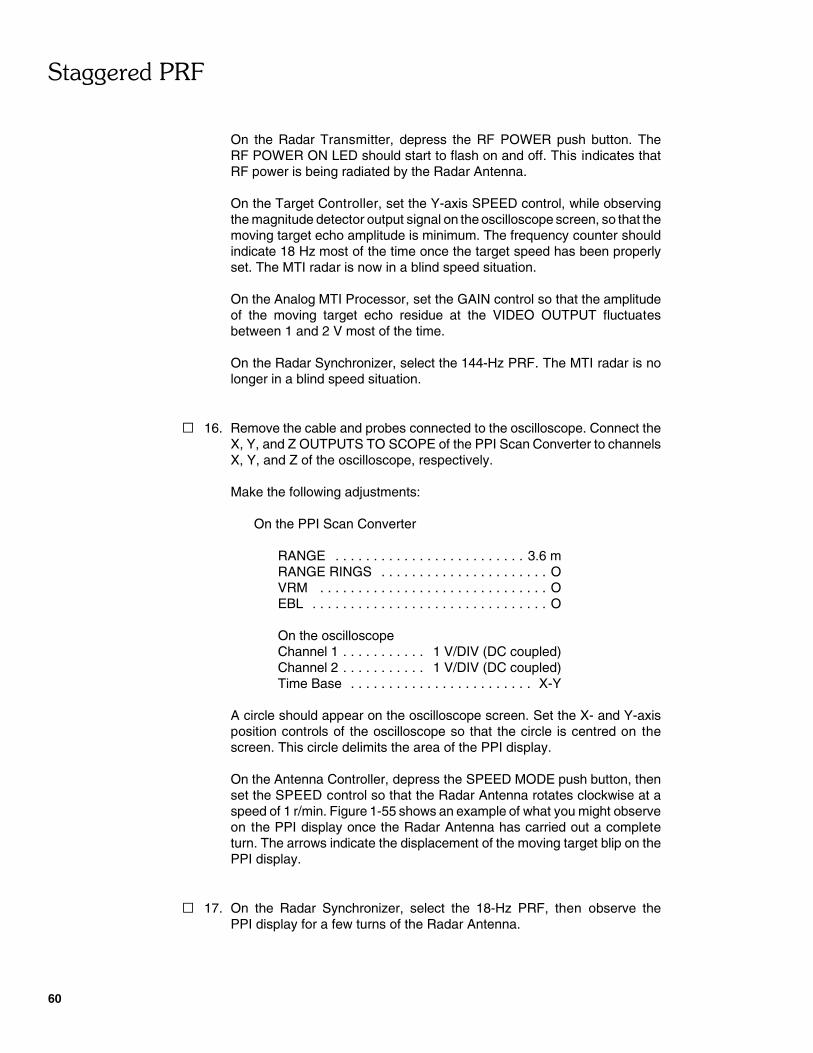
���$$�������&
60
On the Radar Transmitter, depress the RF POWER push button. TheRF POWER ON LED should start to flash on and off. This indicates thatRF power is being radiated by the Radar Antenna.
On the Target Controller, set the Y-axis SPEED control, while observingthe magnitude detector output signal on the oscilloscope screen, so that themoving target echo amplitude is minimum. The frequency counter shouldindicate 18 Hz most of the time once the target speed has been properlyset. The MTI radar is now in a blind speed situation.
On the Analog MTI Processor, set the GAIN control so that the amplitudeof the moving target echo residue at the VIDEO OUTPUT fluctuatesbetween 1 and 2 V most of the time.
On the Radar Synchronizer, select the 144-Hz PRF. The MTI radar is nolonger in a blind speed situation.
� 16. Remove the cable and probes connected to the oscilloscope. Connect theX, Y, and Z OUTPUTS TO SCOPE of the PPI Scan Converter to channelsX, Y, and Z of the oscilloscope, respectively.
Make the following adjustments:
On the PPI Scan Converter
RANGE . . . . . . . . . . . . . . . . . . . . . . . . . 3.6 mRANGE RINGS . . . . . . . . . . . . . . . . . . . . . . OVRM . . . . . . . . . . . . . . . . . . . . . . . . . . . . . . OEBL . . . . . . . . . . . . . . . . . . . . . . . . . . . . . . . O
On the oscilloscopeChannel 1 . . . . . . . . . . . 1 V/DIV (DC coupled)Channel 2 . . . . . . . . . . . 1 V/DIV (DC coupled)Time Base . . . . . . . . . . . . . . . . . . . . . . . . X-Y
A circle should appear on the oscilloscope screen. Set the X- and Y-axisposition controls of the oscilloscope so that the circle is centred on thescreen. This circle delimits the area of the PPI display.
On the Antenna Controller, depress the SPEED MODE push button, thenset the SPEED control so that the Radar Antenna rotates clockwise at aspeed of 1 r/min. Figure 1-55 shows an example of what you might observeon the PPI display once the Radar Antenna has carried out a completeturn. The arrows indicate the displacement of the moving target blip on thePPI display.
� 17. On the Radar Synchronizer, select the 18-Hz PRF, then observe thePPI display for a few turns of the Radar Antenna.

���$$�������&
61
RANGE ..............................................................: 3.6 m
Describe what happens on the PPI display when the PRF is switched from144 to 18 Hz. Explain why.
Figure 1-55. PPI display showing the moving target blip.
On the Radar Synchronizer, select the STAGGERED-PRF MODE, thenobserve the PPI display for a few turns of the Radar Antenna.
Describe what happens on the PPI display when the staggered-PRF modeis enabled. Explain why.
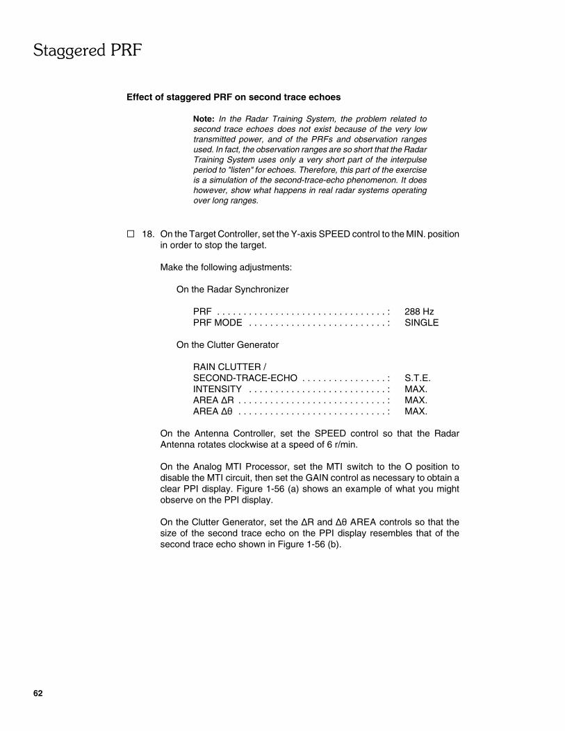
���$$�������&
62
Effect of staggered PRF on second trace echoes
Note: In the Radar Training System, the problem related tosecond trace echoes does not exist because of the very lowtransmitted power, and of the PRFs and observation rangesused. In fact, the observation ranges are so short that the RadarTraining System uses only a very short part of the interpulseperiod to "listen" for echoes. Therefore, this part of the exerciseis a simulation of the second-trace-echo phenomenon. It doeshowever, show what happens in real radar systems operatingover long ranges.
� 18. On the Target Controller, set the Y-axis SPEED control to the MIN. positionin order to stop the target.
Make the following adjustments:
On the Radar Synchronizer
PRF . . . . . . . . . . . . . . . . . . . . . . . . . . . . . . . . : 288 HzPRF MODE . . . . . . . . . . . . . . . . . . . . . . . . . . : SINGLE
On the Clutter Generator
RAIN CLUTTER / SECOND-TRACE-ECHO . . . . . . . . . . . . . . . . : S.T.E.INTENSITY . . . . . . . . . . . . . . . . . . . . . . . . . . : MAX.AREA �R . . . . . . . . . . . . . . . . . . . . . . . . . . . . : MAX.AREA �� . . . . . . . . . . . . . . . . . . . . . . . . . . . . : MAX.
On the Antenna Controller, set the SPEED control so that the RadarAntenna rotates clockwise at a speed of 6 r/min.
On the Analog MTI Processor, set the MTI switch to the O position todisable the MTI circuit, then set the GAIN control as necessary to obtain aclear PPI display. Figure 1-56 (a) shows an example of what you mightobserve on the PPI display.
On the Clutter Generator, set the �R and �� AREA controls so that thesize of the second trace echo on the PPI display resembles that of thesecond trace echo shown in Figure 1-56 (b).
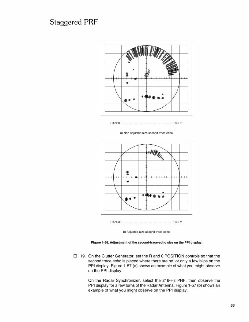
���$$�������&
63
RANGE ..............................................................: 3.6 m
b) Adjusted-size second trace echo
RANGE ..............................................................: 3.6 m
a) Non-adjusted size second trace echo
Figure 1-56. Adjustment of the second-trace-echo size on the PPI display.
� 19. On the Clutter Generator, set the R and � POSITION controls so that thesecond trace echo is placed where there are no, or only a few blips on thePPI display. Figure 1-57 (a) shows an example of what you might observeon the PPI display.
On the Radar Synchronizer, select the 216-Hz PRF, then observe thePPI display for a few turns of the Radar Antenna. Figure 1-57 (b) shows anexample of what you might observe on the PPI display.
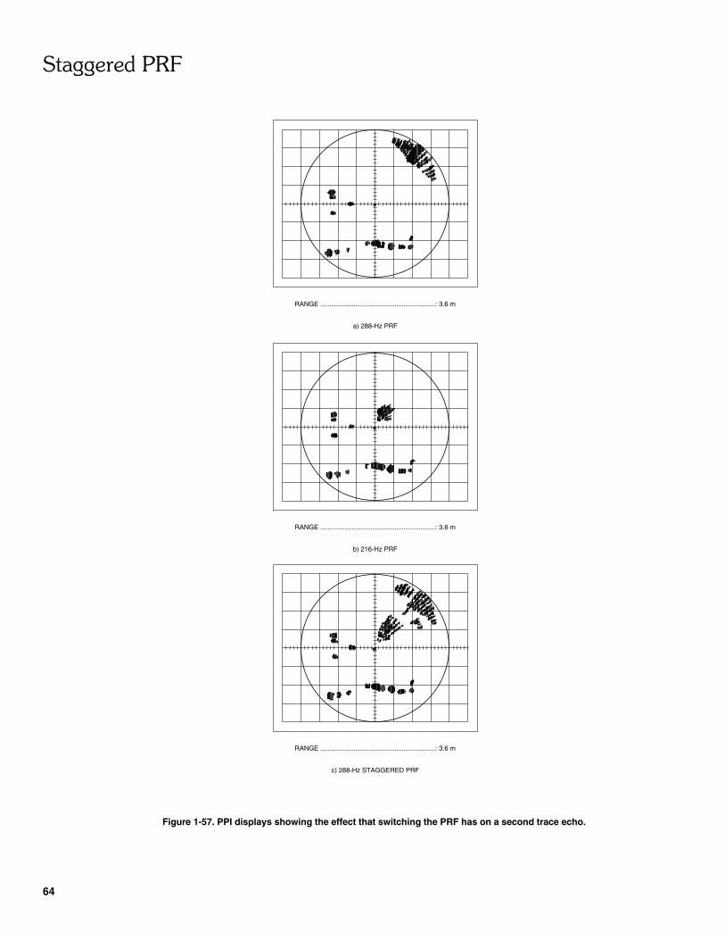
���$$�������&
64
RANGE ..............................................................: 3.6 m
a) 288-Hz PRF
RANGE ..............................................................: 3.6 m
b) 216-Hz PRF
RANGE ..............................................................: 3.6 m
c) 288-Hz STAGGERED PRF
Figure 1-57. PPI displays showing the effect that switching the PRF has on a second trace echo.

���$$�������&
65
Describe what happens on the PPI display when the PRF is switched from288 to 216 Hz.
Explain why this happens on the PPI display when the PRF is switched.
Adjust the Radar Synchronizer as follows:
PRF . . . . . . . . . . . . . . . . . . . . . . . . . . . . 288 HzPRF MODE . . . . . . . . . . . . . . . . . . . STAGGERED
Observe the PPI display for a few turns of the Radar Antenna.Figure 1-57 (c) shows an example of what you might observe on thePPI display.
Describe the effect the staggered-PRF mode has on the second trace echoand other blips on the PPI display.
Explain why the staggered-PRF mode has this effect on the PPI display.

���$$�������&
66
Describe the usefulness of staggered PRF in this situation. Explain why.
� 20. On the Radar Transmitter, make sure that the RF POWER switch is in theSTANDBY position. The RF POWER STANDBY LED should be lit. Placeall POWER switches in the O (off) position and disconnect all cables andaccessories.
CONCLUSION
In this exercise, you found that there is no echo of a moving target at the output ofa phase- or vector-processing MTI radar in a blind speed situation. You observedthat blind speeds are undesirable because the MTI radar sensitivity is considerablyreduced in this situation. You learned that blind speeds occur at the PRF andmultiples of the PRF because the frequency response of the MTI circuit (singledelay-line canceller) is nearly zero at these frequencies. You saw that the use ofstaggered PRF modifies the frequency-response curve of the MTI circuit anddisplaces the first blind speed to a higher frequency which depends on the ratio ofthe PRFs used. You observed that staggered PRF efficiently helps solve theproblem caused by blind speeds.
You learned that a second trace echo is an echo whose round-trip transit time isbetween one and two interpulse periods, and that this kind of echo appears at arange which is smaller than its actual range. You observed that a second trace echoappears at a different range depending on the PRF used and that, instaggered PRF, it appears simultaneously at two different ranges. You finally foundthat staggered PRF is useful in discriminating between normal echoes and secondtrace echoes on a PPI display.
REVIEW QUESTIONS
1. What are blind speeds?

���$$�������&
67
2. What is the first blind speed of a radar whose transmitted frequency is500 MHz, and whose pulse-repetition rate is 500 Hz?
3. Why is the range of a second-trace echo ambiguous?
4. What is the effect of staggered PRF on blind speeds? Explain.
5. What is the effect of staggered PRF on second-trace echoes?


���������������
����
"�$�����%�"���������$

71
�����������
���!�������"���#�$�������%���������
EXERCISE OBJECTIVE
When you have completed this exercise, you will be familiar with the methods usedto process target reports in order to track a number of moving targets simulta-neously while the antenna is rotating.
DISCUSSION
The third and final stage in MTD processing is surveillance, or track-while-scan,processing. This uses scan-to-scan target history to track moving targets whilefiltering out undesired reports.
When surveillance processing is used, each tracked target is represented on theradar display by a symbol which indicates the target direction, and a code whichidentifies the target. Additional information may also displayed, such as targetspeed, range, and azimuth.
Processing steps
The surveillance process consists of a number of steps, shown in Figure 3-4. Thepurpose of each step is given below.
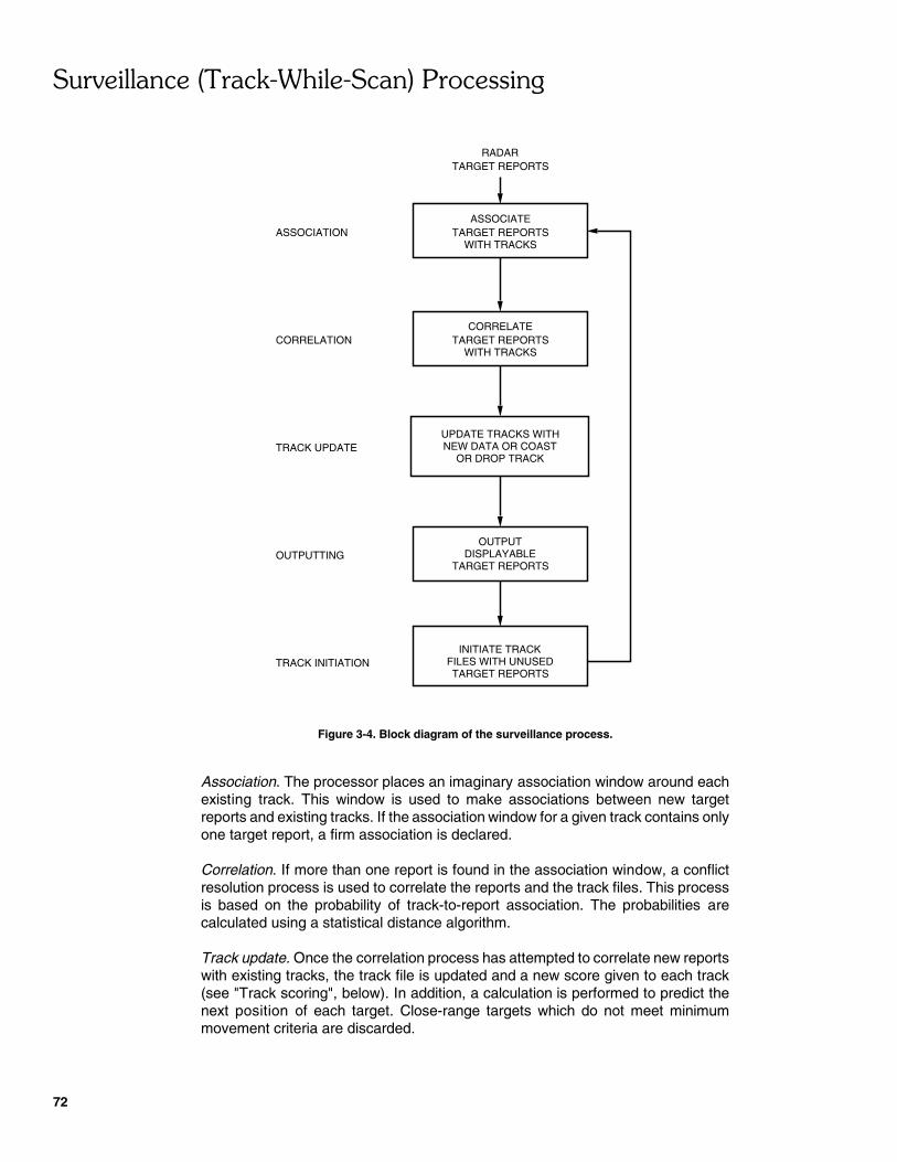
���'�������� ����()*!���)�������������$
72
TARGET REPORTS
INITIATE TRACKFILES WITH UNUSEDTARGET REPORTS
TARGET REPORTS
UPDATE TRACKS WITHNEW DATA OR COAST
OR DROP TRACK
TARGET REPORTSWITH TRACKS
WITH TRACKSTARGET REPORTS
TRACK INITIATION
OUTPUTTING
TRACK UPDATE
CORRELATION
ASSOCIATION
DISPLAYABLEOUTPUT
CORRELATE
ASSOCIATE
RADAR
Figure 3-4. Block diagram of the surveillance process.
Association. The processor places an imaginary association window around eachexisting track. This window is used to make associations between new targetreports and existing tracks. If the association window for a given track contains onlyone target report, a firm association is declared.
Correlation. If more than one report is found in the association window, a conflictresolution process is used to correlate the reports and the track files. This processis based on the probability of track-to-report association. The probabilities arecalculated using a statistical distance algorithm.
Track update. Once the correlation process has attempted to correlate new reportswith existing tracks, the track file is updated and a new score given to each track(see "Track scoring", below). In addition, a calculation is performed to predict thenext position of each target. Close-range targets which do not meet minimummovement criteria are discarded.
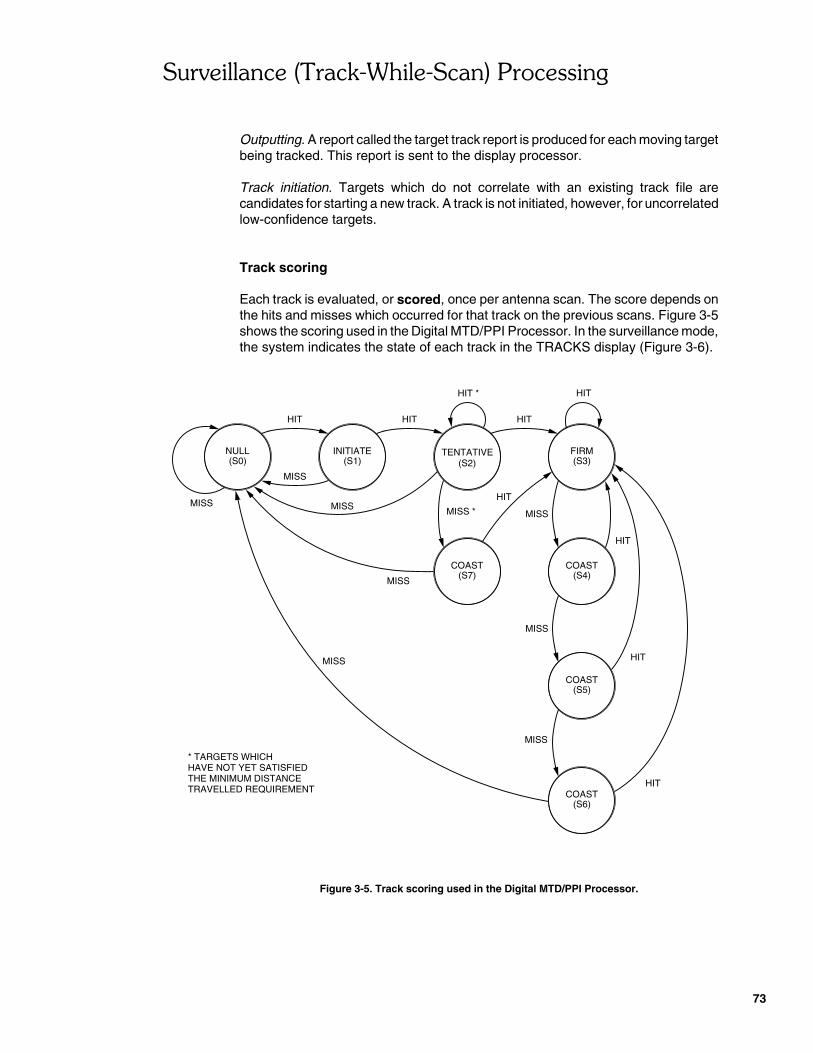
���'�������� ����()*!���)�������������$
73
TRAVELLED REQUIREMENTTHE MINIMUM DISTANCEHAVE NOT YET SATISFIED* TARGETS WHICH
NULL
MISS
HITHIT
MISS
(S0)
MISS
MISS
MISS
INITIATE(S1)
MISS
(S6)COAST
COAST(S5)
HIT
HIT
HIT
MISS
MISS
COAST(S7)
TENTATIVE
MISS *
(S2)
HIT
COAST(S4)
FIRM(S3)
HIT
HIT * HIT
Outputting. A report called the target track report is produced for each moving targetbeing tracked. This report is sent to the display processor.
Track initiation. Targets which do not correlate with an existing track file arecandidates for starting a new track. A track is not initiated, however, for uncorrelatedlow-confidence targets.
Track scoring
Each track is evaluated, or scored, once per antenna scan. The score depends onthe hits and misses which occurred for that track on the previous scans. Figure 3-5shows the scoring used in the Digital MTD/PPI Processor. In the surveillance mode,the system indicates the state of each track in the TRACKS display (Figure 3-6).
Figure 3-5. Track scoring used in the Digital MTD/PPI Processor.
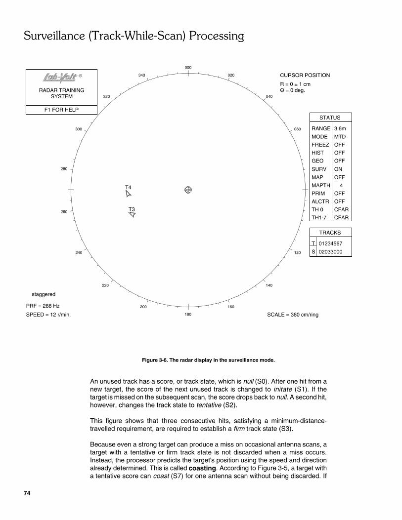
���'�������� ����()*!���)�������������$
74
000
020
040
060
340
320
300
180
160
140
120240
220
200
280
260
RADAR TRAININGSYSTEM
F1 FOR HELP
CURSOR POSITION
R = 0 ± 1 cmÞ = 0 deg.
SPEED = 12 r/min.
PRF = 288 Hz
SCALE = 360 cm/ring
T3
T4
TH1-7
TH 0
ALCTR
PRIM
MAPTH
MAP
SURV
CFAR
CFAR
OFF
OFF
OFF
4
ON
GEO
HIST
FREEZ
MODE
RANGE 3.6m
OFF
OFF
OFF
MTD
STATUS
staggered
TRACKS
01234567T
S 02033000
Figure 3-6. The radar display in the surveillance mode.
An unused track has a score, or track state, which is null (S0). After one hit from anew target, the score of the next unused track is changed to initate (S1). If thetarget is missed on the subsequent scan, the score drops back to null. A second hit,however, changes the track state to tentative (S2).
This figure shows that three consecutive hits, satisfying a minimum-distance-travelled requirement, are required to establish a firm track state (S3).
Because even a strong target can produce a miss on occasional antenna scans, atarget with a tentative or firm track state is not discarded when a miss occurs.Instead, the processor predicts the target's position using the speed and directionalready determined. This is called coasting. According to Figure 3-5, a target witha tentative score can coast (S7) for one antenna scan without being discarded. If
���'�������� ����()*!���)�������������$
75
the target is not detected on the next scan, however, the track is discarded, and thescore for that track is returned to null. A target with a firm track can coast for threeantenna scans (S4, S5, and S6) without being discarded. If a miss occurs on thefourth scan, however, the track is discarded.
NEW FUNCTIONS
KEY FUNCTION NAME EFFECT STATUS DISPLAY MODE
F7 SURVEILLANCE Switches surveillance on or off SURV � ON/OFF MTD
PROCEDURE
Set-up and calibration
� 1. Before beginning this exercise, the main elements of the Radar TrainingSystem (the antenna, the target table, and the training modules) must beset up as shown in Appendix A.
Set up and connect the modules as shown in Appendix B.
� 2. Calibrate the digital radar according to the instructions in Appendix C.
Note: Since the radiation levels of the Radar Training Systemare very low, there is no danger to anyone standing near or infront of the antenna. Remember, however, that with a full-scaleradar, you must always make sure that no one could be exposedto dangerous radiation levels before turning on the RF power.
Adjustments
� 3. Make the following adjustments:
On the Radar Transmitter
RF OSCILLATOR FREQUENCY . . . . . . . CAL.PULSE GENERATOR PULSE WIDTH . . 1 nsRF POWER . . . . . . . . . . . . . . . . . . . . . . . . ON
On the Clutter Generator
SEA CLUTTER . . . . . . . . . . . . . . . . . . . . OFFRAIN CLUTTER /
SECOND-TRACE-ECHO . . . . . . . . . . . . . . OFFINTERFERENCE / NOISE . . . . . . . . . . . OFF
���'�������� ����()*!���)�������������$
76
On the Radar Synchronizer
PRF . . . . . . . . . . . . . . . . . . . . . . . . . . . 288 HzPRF MODE . . . . . . . . . . . . . . . STAGGERED
On the Antenna Controller
ANTENNA ROTATION MODE . . . PRF LOCK.
On the Dual-Channel Sampler
RANGE SPAN . . . . . . . . . . . . . . . . . . . . 3.6 m
On the Digital MTD/PPI Processor
STC . . . . . . . . . . . . . . . . . . . . . . . . . . . . . . . OBASELINE ADJUSTMENT UPDATE . . . . . . . IMODE . . . . . . . . . . . . . . . . . . . . . . . . . . MTDRANGE . . . . . . . . . . . . . . . . . . . . . . . . . 3.6 m
� 4. Position the target table so it is approximately 0.5 m from the Rotating-Antenna Pedestal. Place a half-cylinder target on the mast of the targettable. Adjust the Target Controller so the target moves in a circulartrajectory at low speed.
Tracking targets
� 5. Turn on the SURVEILLANCE function (press F7) and observe the display.After a large number of antenna rotations, a track is established, and thetarget is represented by an arrowhead. A target number Tn is assigned tothe target. Observe the radar display as the target is tracked around itstrajectory.
Refer to Figure 3-6 and observe the states of the various tracks in theTRACKS display or the radar monitor.
� 6. Install the two-target adapter on the target table, with two half-cylindertargets separated by approximately 65 cm, as shown in Figure 3-7. Makethe targets move in a circular trajectory at a very low speed (approximately2 cm/s). Describe what you observe on the display.
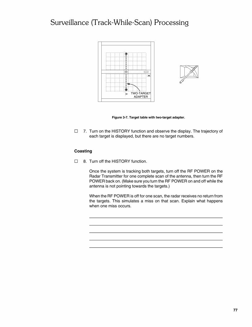
���'�������� ����()*!���)�������������$
77
Y
X
TWO-TARGETADAPTER
Figure 3-7. Target table with two-target adapter.
� 7. Turn on the HISTORY function and observe the display. The trajectory ofeach target is displayed, but there are no target numbers.
Coasting
� 8. Turn off the HISTORY function.
Once the system is tracking both targets, turn off the RF POWER on theRadar Transmitter for one complete scan of the antenna, then turn the RFPOWER back on. (Make sure you turn the RF POWER on and off while theantenna is not pointing towards the targets.)
When the RF POWER is off for one scan, the radar receives no return fromthe targets. This simulates a miss on that scan. Explain what happenswhen one miss occurs.

���'�������� ����()*!���)�������������$
78
Y
X
� 9. Repeat the previous step several times. Under what conditions does thesurveillance processor successfully resume tracking? What happens whentracking cannot be resumed?
� 10. With the processor tracking both targets, turn off the RF POWER for twocomplete antenna scans. Observe under what conditions a track ismaintained and when it is lost.
Turn off the RF POWER for three complete antenna scans. Note that theDigital MTD/PPI Processor usually loses the track after three successivemisses.
� 11. Turn the two-target adapter so one target masks the other at a certain pointin the trajectory, as shown in Figure 3-8. Orient the half-cylinder targets asshown in the Figure. Make the targets move in a circular trajectory at lowspeed.
Observe what happens when the far target is masked by the near target.
Figure 3-8. One target masking the other.
� 12. On the Radar Transmitter, make sure that the RF POWER switch is in theSTANDBY position. The RF POWER STANDBY LED should be lit. Turn offall equipment.
���'�������� ����()*!���)�������������$
79
CONCLUSION
In this exercise you observed that the digital radar system can track several targetssimultaneously. You observed that each track is scored once per antenna scan.When a miss occurs in a track, the target is allowed to coast. After a certain numberof misses, the track is discarded.


���������������
����
����(�$������

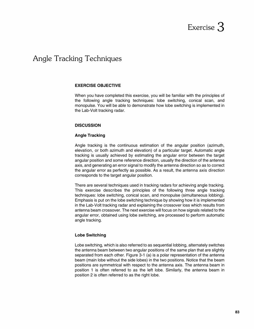
83
���������
&�������#�������'���
EXERCISE OBJECTIVE
When you have completed this exercise, you will be familiar with the principles ofthe following angle tracking techniques: lobe switching, conical scan, andmonopulse. You will be able to demonstrate how lobe switching is implemented inthe Lab-Volt tracking radar.
DISCUSSION
Angle Tracking
Angle tracking is the continuous estimation of the angular position (azimuth,elevation, or both azimuth and elevation) of a particular target. Automatic angletracking is usually achieved by estimating the angular error between the targetangular position and some reference direction, usually the direction of the antennaaxis, and generating an error signal to modify the antenna direction so as to correctthe angular error as perfectly as possible. As a result, the antenna axis directioncorresponds to the target angular position.
There are several techniques used in tracking radars for achieving angle tracking.This exercise describes the principles of the following three angle trackingtechniques: lobe switching, conical scan, and monopulse (simultaneous lobbing).Emphasis is put on the lobe switching technique by showing how it is implementedin the Lab-Volt tracking radar and explaining the crossover loss which results fromantenna beam crossover. The next exercise will focus on how signals related to theangular error, obtained using lobe switching, are processed to perform automaticangle tracking.
Lobe Switching
Lobe switching, which is also referred to as sequential lobbing, alternately switchesthe antenna beam between two angular positions of the same plan that are slightlyseparated from each other. Figure 3-1 (a) is a polar representation of the antennabeam (main lobe without the side lobes) in the two positions. Notice that the beampositions are symmetrical with respect to the antenna axis. The antenna beam inposition 1 is often referred to as the left lobe. Similarly, the antenna beam inposition 2 is often referred to as the right lobe.
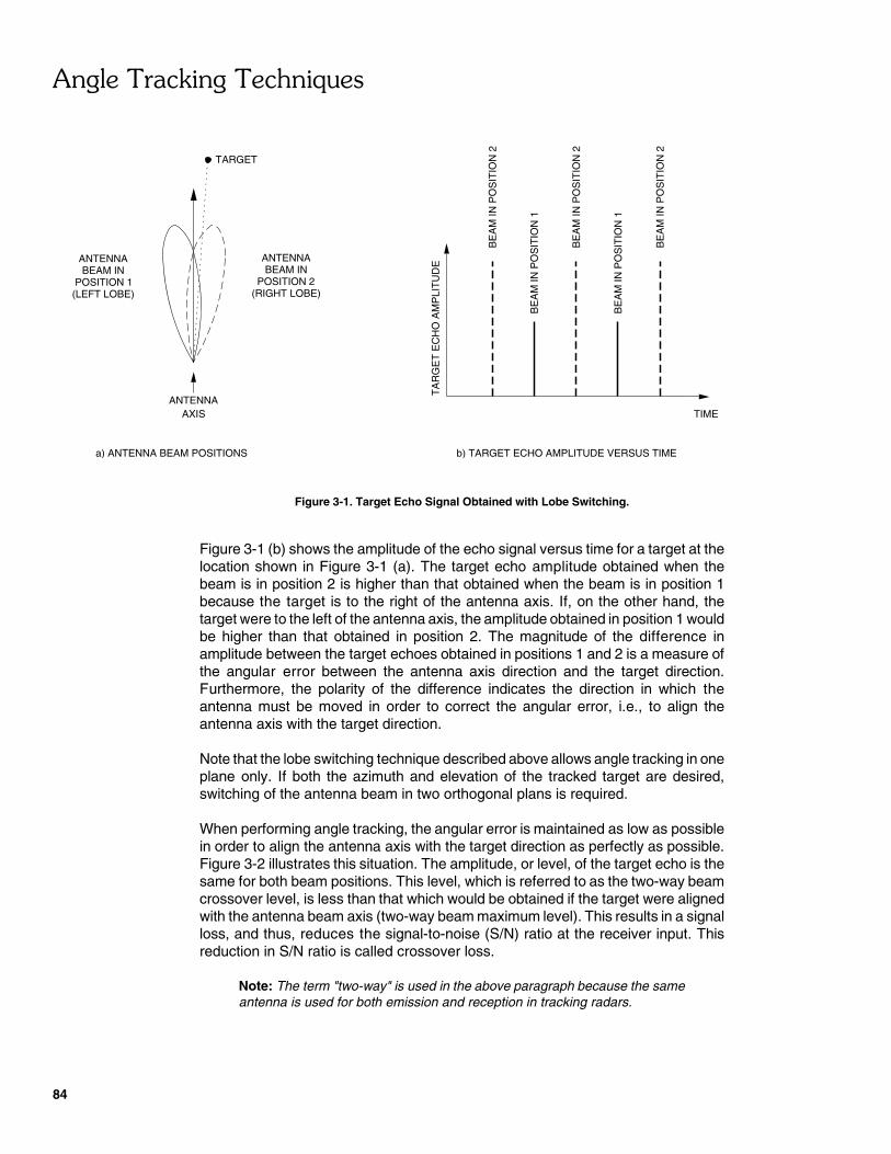
#$�������(�$����!�+���
84
b) TARGET ECHO AMPLITUDE VERSUS TIME
TA
RG
ET
EC
HO
AM
PLI
TU
DE
TIME
a) ANTENNA BEAM POSITIONS
ANTENNAAXIS
ANTENNABEAM IN
POSITION 1(LEFT LOBE) (RIGHT LOBE)
POSITION 2
ANTENNABEAM IN
TARGET
BE
AM
IN P
OS
ITIO
N 2
BE
AM
IN P
OS
ITIO
N 2
BE
AM
IN P
OS
ITIO
N 2
BE
AM
IN P
OS
ITIO
N 1
BE
AM
IN P
OS
ITIO
N 1
Figure 3-1. Target Echo Signal Obtained with Lobe Switching.
Figure 3-1 (b) shows the amplitude of the echo signal versus time for a target at thelocation shown in Figure 3-1 (a). The target echo amplitude obtained when thebeam is in position 2 is higher than that obtained when the beam is in position 1because the target is to the right of the antenna axis. If, on the other hand, thetarget were to the left of the antenna axis, the amplitude obtained in position 1 wouldbe higher than that obtained in position 2. The magnitude of the difference inamplitude between the target echoes obtained in positions 1 and 2 is a measure ofthe angular error between the antenna axis direction and the target direction.Furthermore, the polarity of the difference indicates the direction in which theantenna must be moved in order to correct the angular error, i.e., to align theantenna axis with the target direction.
Note that the lobe switching technique described above allows angle tracking in oneplane only. If both the azimuth and elevation of the tracked target are desired,switching of the antenna beam in two orthogonal plans is required.
When performing angle tracking, the angular error is maintained as low as possiblein order to align the antenna axis with the target direction as perfectly as possible.Figure 3-2 illustrates this situation. The amplitude, or level, of the target echo is thesame for both beam positions. This level, which is referred to as the two-way beamcrossover level, is less than that which would be obtained if the target were alignedwith the antenna beam axis (two-way beam maximum level). This results in a signalloss, and thus, reduces the signal-to-noise (S/N) ratio at the receiver input. Thisreduction in S/N ratio is called crossover loss.
Note: The term "two-way" is used in the above paragraph because the sameantenna is used for both emission and reception in tracking radars.
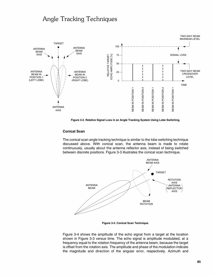
#$�������(�$����!�+���
85
EC
HO
AM
PLI
TU
DE
[%]
TIME
ANTENNAAXIS
ANTENNABEAM IN
POSITION 1(LEFT LOBE) (RIGHT LOBE)
POSITION 2
ANTENNABEAM IN
TARGET
BE
AM
IN P
OS
ITIO
N 1
BE
AM
IN P
OS
ITIO
N 1
BE
AM
IN P
OS
ITIO
N 1
BE
AM
IN P
OS
ITIO
N 2
BE
AM
IN P
OS
ITIO
N 2
0
25
50
75
100
RE
LAT
IVE
TA
RG
ET SIGNAL LOSS
TWO-WAY BEAMMAXIMUM LEVEL
AXIS
ANTENNABEAM
AXIS
ANTENNABEAM
TWO-WAY BEAMCROSSOVER
LEVEL
TARGET
ANTENNABEAM
BEAMROTATION
ANTENNABEAM AXIS
ROTATIONAXIS
ANTENNAREFLECTOR
AXIS
Figure 3-2. Relative Signal Loss in an Angle Tracking System Using Lobe Switching.
Conical Scan
The conical scan angle tracking technique is similar to the lobe switching techniquediscussed above. With conical scan, the antenna beam is made to rotatecontinuously, usually about the antenna reflector axis, instead of being switchedbetween discrete positions. Figure 3-3 illustrates the conical scan technique.
Figure 3-3. Conical Scan Technique.
Figure 3-4 shows the amplitude of the echo signal from a target at the locationshown in Figure 3-3 versus time. The echo signal is amplitude modulated, at afrequency equal to the rotation frequency of the antenna beam, because the targetis offset from the rotation axis. The amplitude and phase of the modulation indicatethe magnitude and direction of the angular error, respectively. Azimuth and
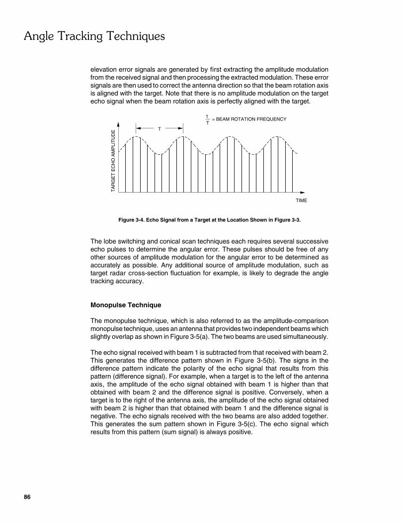
#$�������(�$����!�+���
86
TA
RG
ET
EC
HO
AM
PLI
TU
DE
TIME
T
= BEAM ROTATION FREQUENCY1T
elevation error signals are generated by first extracting the amplitude modulationfrom the received signal and then processing the extracted modulation. These errorsignals are then used to correct the antenna direction so that the beam rotation axisis aligned with the target. Note that there is no amplitude modulation on the targetecho signal when the beam rotation axis is perfectly aligned with the target.
Figure 3-4. Echo Signal from a Target at the Location Shown in Figure 3-3.
The lobe switching and conical scan techniques each requires several successiveecho pulses to determine the angular error. These pulses should be free of anyother sources of amplitude modulation for the angular error to be determined asaccurately as possible. Any additional source of amplitude modulation, such astarget radar cross-section fluctuation for example, is likely to degrade the angletracking accuracy.
Monopulse Technique
The monopulse technique, which is also referred to as the amplitude-comparisonmonopulse technique, uses an antenna that provides two independent beams whichslightly overlap as shown in Figure 3-5(a). The two beams are used simultaneously.
The echo signal received with beam 1 is subtracted from that received with beam 2.This generates the difference pattern shown in Figure 3-5(b). The signs in thedifference pattern indicate the polarity of the echo signal that results from thispattern (difference signal). For example, when a target is to the left of the antennaaxis, the amplitude of the echo signal obtained with beam 1 is higher than thatobtained with beam 2 and the difference signal is positive. Conversely, when atarget is to the right of the antenna axis, the amplitude of the echo signal obtainedwith beam 2 is higher than that obtained with beam 1 and the difference signal isnegative. The echo signals received with the two beams are also added together.This generates the sum pattern shown in Figure 3-5(c). The echo signal whichresults from this pattern (sum signal) is always positive.
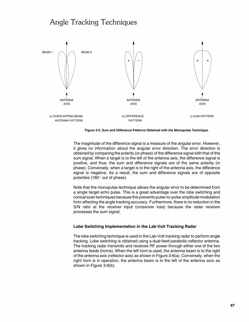
#$�������(�$����!�+���
87
a) OVERLAPPING-BEAM
ANTENNAAXIS
BEAM 1 BEAM 2
ANTENNA PATTERN
ANTENNAAXIS
ANTENNAAXIS
+ −
PATTERN
b) DIFFERENCE
+ +
c) SUM PATTERN
Figure 3-5. Sum and Difference Patterns Obtained with the Monopulse Technique.
The magnitude of the difference signal is a measure of the angular error. However,it gives no information about the angular error direction. The error direction isobtained by comparing the polarity (or phase) of the difference signal with that of thesum signal. When a target is to the left of the antenna axis, the difference signal ispositive, and thus, the sum and difference signals are of the same polarity (inphase). Conversely, when a target is to the right of the antenna axis, the differencesignal is negative. As a result, the sum and difference signals are of oppositepolarities (180� out of phase).
Note that the monopulse technique allows the angular error to be determined froma single target echo pulse. This is a great advantage over the lobe switching andconical scan techniques because this prevents pulse-to-pulse amplitude modulationfrom affecting the angle tracking accuracy. Furthermore, there is no reduction in theS/N ratio at the receiver input (crossover loss) because the radar receiverprocesses the sum signal.
Lobe Switching Implementation in the Lab-Volt Tracking Radar
The lobe switching technique is used in the Lab-Volt tracking radar to perform angletracking. Lobe switching is obtained using a dual-feed parabolic-reflector antenna.The tracking radar transmits and receives RF power through either one of the twoantenna feeds (horns). When the left horn is used, the antenna beam is to the rightof the antenna axis (reflector axis) as shown in Figure 3-6(a). Conversely, when theright horn is in operation, the antenna beam is to the left of the antenna axis asshown in Figure 3-6(b).
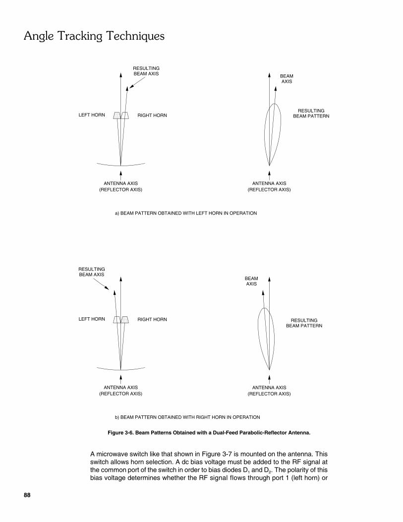
#$�������(�$����!�+���
88
ANTENNA AXIS(REFLECTOR AXIS)
LEFT HORN RIGHT HORN
RESULTINGBEAM AXIS BEAM
AXIS
(REFLECTOR AXIS)ANTENNA AXIS
(REFLECTOR AXIS)ANTENNA AXIS
BEAMAXIS
a) BEAM PATTERN OBTAINED WITH LEFT HORN IN OPERATION
b) BEAM PATTERN OBTAINED WITH RIGHT HORN IN OPERATION
LEFT HORN RIGHT HORN
ANTENNA AXIS(REFLECTOR AXIS)
BEAM AXISRESULTING
RESULTINGBEAM PATTERN
BEAM PATTERNRESULTING
Figure 3-6. Beam Patterns Obtained with a Dual-Feed Parabolic-Reflector Antenna.
A microwave switch like that shown in Figure 3-7 is mounted on the antenna. Thisswitch allows horn selection. A dc bias voltage must be added to the RF signal atthe common port of the switch in order to bias diodes D1 and D2. The polarity of thisbias voltage determines whether the RF signal flows through port 1 (left horn) or
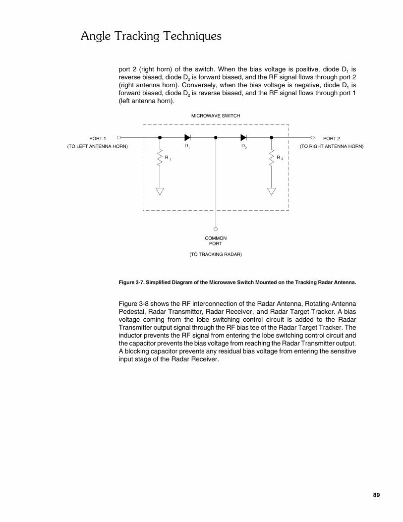
#$�������(�$����!�+���
89
(TO LEFT ANTENNA HORN) D1 D2
PORT 1
(TO RIGHT ANTENNA HORN)
PORT 2
MICROWAVE SWITCH
COMMONPORT
(TO TRACKING RADAR)
R 1 R 2
port 2 (right horn) of the switch. When the bias voltage is positive, diode D1 isreverse biased, diode D2 is forward biased, and the RF signal flows through port 2(right antenna horn). Conversely, when the bias voltage is negative, diode D1 isforward biased, diode D2 is reverse biased, and the RF signal flows through port 1(left antenna horn).
Figure 3-7. Simplified Diagram of the Microwave Switch Mounted on the Tracking Radar Antenna.
Figure 3-8 shows the RF interconnection of the Radar Antenna, Rotating-AntennaPedestal, Radar Transmitter, Radar Receiver, and Radar Target Tracker. A biasvoltage coming from the lobe switching control circuit is added to the RadarTransmitter output signal through the RF bias tee of the Radar Target Tracker. Theinductor prevents the RF signal from entering the lobe switching control circuit andthe capacitor prevents the bias voltage from reaching the Radar Transmitter output.A blocking capacitor prevents any residual bias voltage from entering the sensitiveinput stage of the Radar Receiver.
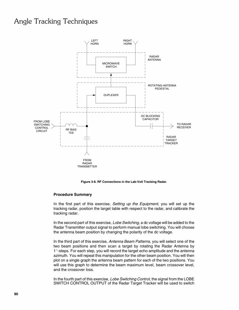
#$�������(�$����!�+���
90
MICROWAVESWITCH
DUPLEXER
LEFTHORN
RIGHTHORN
RF BIASTEE
DC BLOCKINGCAPACITOR
TO RADARRECEIVER
RADARTARGET
TRACKER
FROM LOBESWITCHINGCONTROLCIRCUIT
FROMRADAR
TRANSMITTER
ROTATING-ANTENNAPEDESTAL
RADARANTENNA
Figure 3-8. RF Connections in the Lab-Volt Tracking Radar.
Procedure Summary
In the first part of this exercise, Setting up the Equipment, you will set up thetracking radar, position the target table with respect to the radar, and calibrate thetracking radar.
In the second part of this exercise, Lobe Switching, a dc voltage will be added to theRadar Transmitter output signal to perform manual lobe switching. You will choosethe antenna beam position by changing the polarity of the dc voltage.
In the third part of this exercise, Antenna Beam Patterns, you will select one of thetwo beam positions and then scan a target by rotating the Radar Antenna by1�-steps. For each step, you will record the target echo amplitude and the antennaazimuth. You will repeat this manipulation for the other beam position. You will thenplot on a single graph the antenna beam pattern for each of the two positions. Youwill use this graph to determine the beam maximum level, beam crossover level,and the crossover loss.
In the fourth part of this exercise, Lobe Switching Control, the signal from the LOBESWITCH CONTROL OUTPUT of the Radar Target Tracker will be used to switch
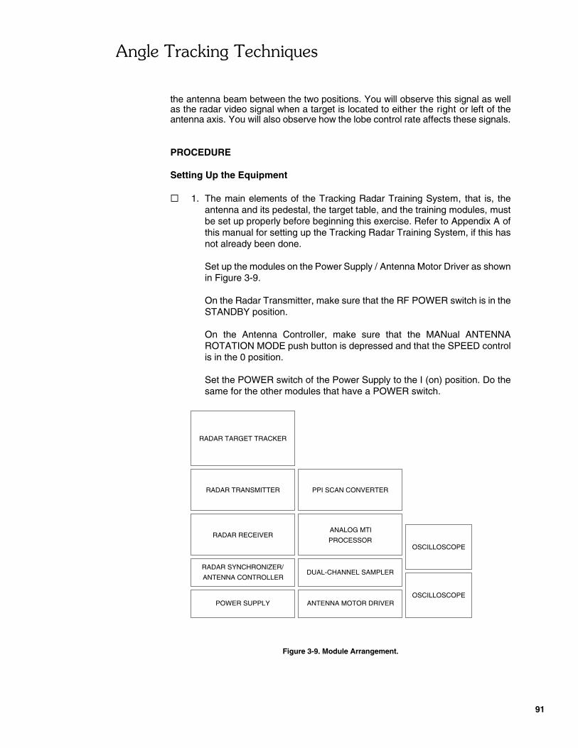
#$�������(�$����!�+���
91
RADAR SYNCHRONIZER/DUAL-CHANNEL SAMPLER
OSCILLOSCOPE
RADAR RECEIVER
PPI SCAN CONVERTERRADAR TRANSMITTER
RADAR TARGET TRACKER
ANTENNA CONTROLLER
ANTENNA MOTOR DRIVERPOWER SUPPLY
PROCESSOR
ANALOG MTI
OSCILLOSCOPE
the antenna beam between the two positions. You will observe this signal as wellas the radar video signal when a target is located to either the right or left of theantenna axis. You will also observe how the lobe control rate affects these signals.
PROCEDURE
Setting Up the Equipment
� 1. The main elements of the Tracking Radar Training System, that is, theantenna and its pedestal, the target table, and the training modules, mustbe set up properly before beginning this exercise. Refer to Appendix A ofthis manual for setting up the Tracking Radar Training System, if this hasnot already been done.
Set up the modules on the Power Supply / Antenna Motor Driver as shownin Figure 3-9.
On the Radar Transmitter, make sure that the RF POWER switch is in theSTANDBY position.
On the Antenna Controller, make sure that the MANual ANTENNAROTATION MODE push button is depressed and that the SPEED controlis in the 0 position.
Set the POWER switch of the Power Supply to the I (on) position. Do thesame for the other modules that have a POWER switch.
Figure 3-9. Module Arrangement.
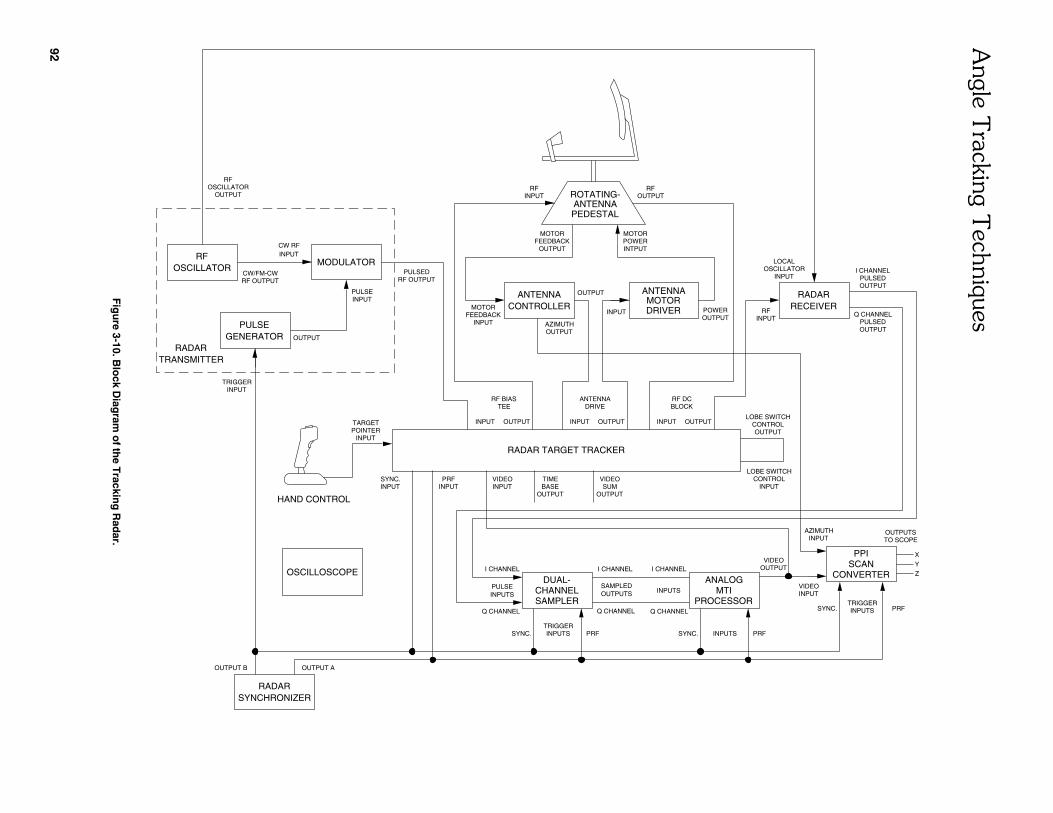
#$�������(
�$����!
�+���
92
RADAR TARGET TRACKER
SYNC.INPUT
PRFINPUT INPUT
VIDEO TIMEBASE
OUTPUT OUTPUTSUM
VIDEO
INPUTPOINTERTARGET
LOBE SWITCHCONTROLOUTPUT
LOBE SWITCHCONTROL
INPUT
INPUT OUTPUT
TEERF BIAS
DRIVEANTENNA
OUTPUTINPUT
BLOCKRF DC
OUTPUTINPUT
ANTENNACONTROLLER
ANTENNAMOTORDRIVER
AZIMUTHOUTPUT
OUTPUT
INPUT POWEROUTPUT
RECEIVERRADAR
RFINPUT
LOCALOSCILLATOR
INPUT
Q CHANNELPULSEDOUTPUT
OUTPUTPULSED
I CHANNEL
ROTATING-ANTENNAPEDESTAL
FEEDBACKMOTOR
INPUT
FEEDBACKMOTOR
OUTPUT INTPUTPOWERMOTOR
CHANNELDUAL-
INPUTS
INPUTSTRIGGER
Q CHANNELSAMPLER
PULSE
I CHANNEL
Q CHANNEL
SYNC. PRF
SAMPLEDOUTPUTS
I CHANNEL
SYNC.
Q CHANNEL
I CHANNEL
INPUTS MTIPROCESSOR
INPUTS PRF
ANALOGOUTPUTVIDEO
CONVERTER
PPISCAN
PRFTRIGGERINPUTSSYNC.
INPUTAZIMUTH OUTPUTS
TO SCOPE
X
Y
Z
RADARSYNCHRONIZER
OSCILLOSCOPE
HAND CONTROL
OUTPUT B OUTPUT A
INPUTRF
OUTPUTRF
RFOSCILLATOR
CW/FM-CWRF OUTPUT
INPUTMODULATOR
PULSEDRF OUTPUT
CW RF
GENERATORPULSE
OUTPUTOSCILLATOR
RF
TRIGGERINPUT
TRANSMITTERRADAR
INPUTPULSE
OUTPUT
INPUTVIDEO
Fig
ure 3-10. B
lock D
iagram
of th
e Trackin
g R
adar.
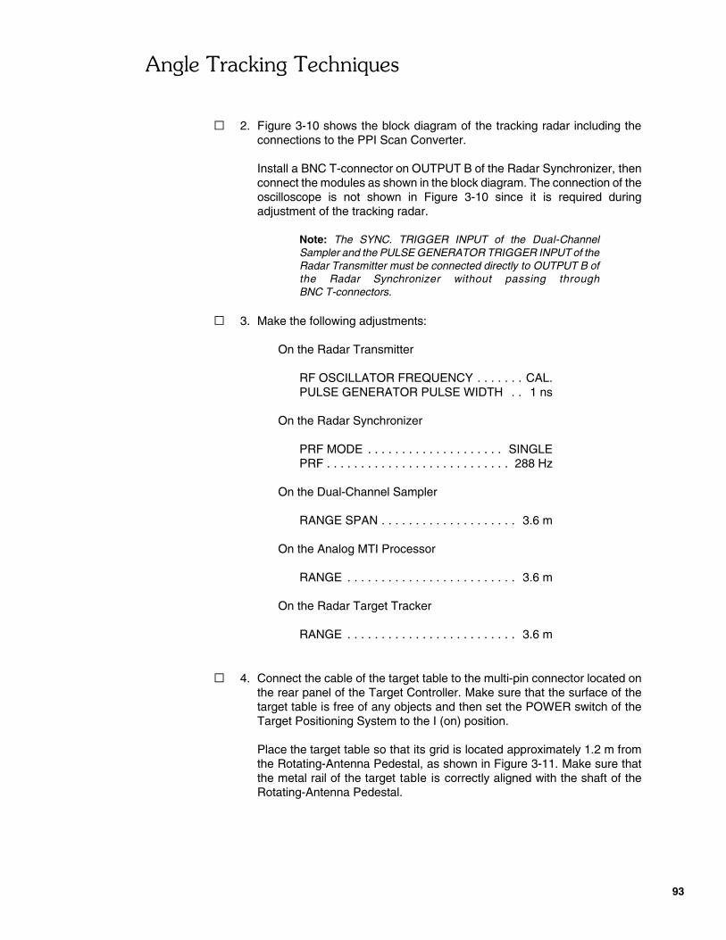
#$�������(�$����!�+���
93
� 2. Figure 3-10 shows the block diagram of the tracking radar including theconnections to the PPI Scan Converter.
Install a BNC T-connector on OUTPUT B of the Radar Synchronizer, thenconnect the modules as shown in the block diagram. The connection of theoscilloscope is not shown in Figure 3-10 since it is required duringadjustment of the tracking radar.
Note: The SYNC. TRIGGER INPUT of the Dual-ChannelSampler and the PULSE GENERATOR TRIGGER INPUT of theRadar Transmitter must be connected directly to OUTPUT B ofthe Radar Synchronizer without passing throughBNC T-connectors.
� 3. Make the following adjustments:
On the Radar Transmitter
RF OSCILLATOR FREQUENCY . . . . . . . CAL.PULSE GENERATOR PULSE WIDTH . . 1 ns
On the Radar Synchronizer
PRF MODE . . . . . . . . . . . . . . . . . . . . SINGLEPRF . . . . . . . . . . . . . . . . . . . . . . . . . . . 288 Hz
On the Dual-Channel Sampler
RANGE SPAN . . . . . . . . . . . . . . . . . . . . 3.6 m
On the Analog MTI Processor
RANGE . . . . . . . . . . . . . . . . . . . . . . . . . 3.6 m
On the Radar Target Tracker
RANGE . . . . . . . . . . . . . . . . . . . . . . . . . 3.6 m
� 4. Connect the cable of the target table to the multi-pin connector located onthe rear panel of the Target Controller. Make sure that the surface of thetarget table is free of any objects and then set the POWER switch of theTarget Positioning System to the I (on) position.
Place the target table so that its grid is located approximately 1.2 m fromthe Rotating-Antenna Pedestal, as shown in Figure 3-11. Make sure thatthe metal rail of the target table is correctly aligned with the shaft of theRotating-Antenna Pedestal.
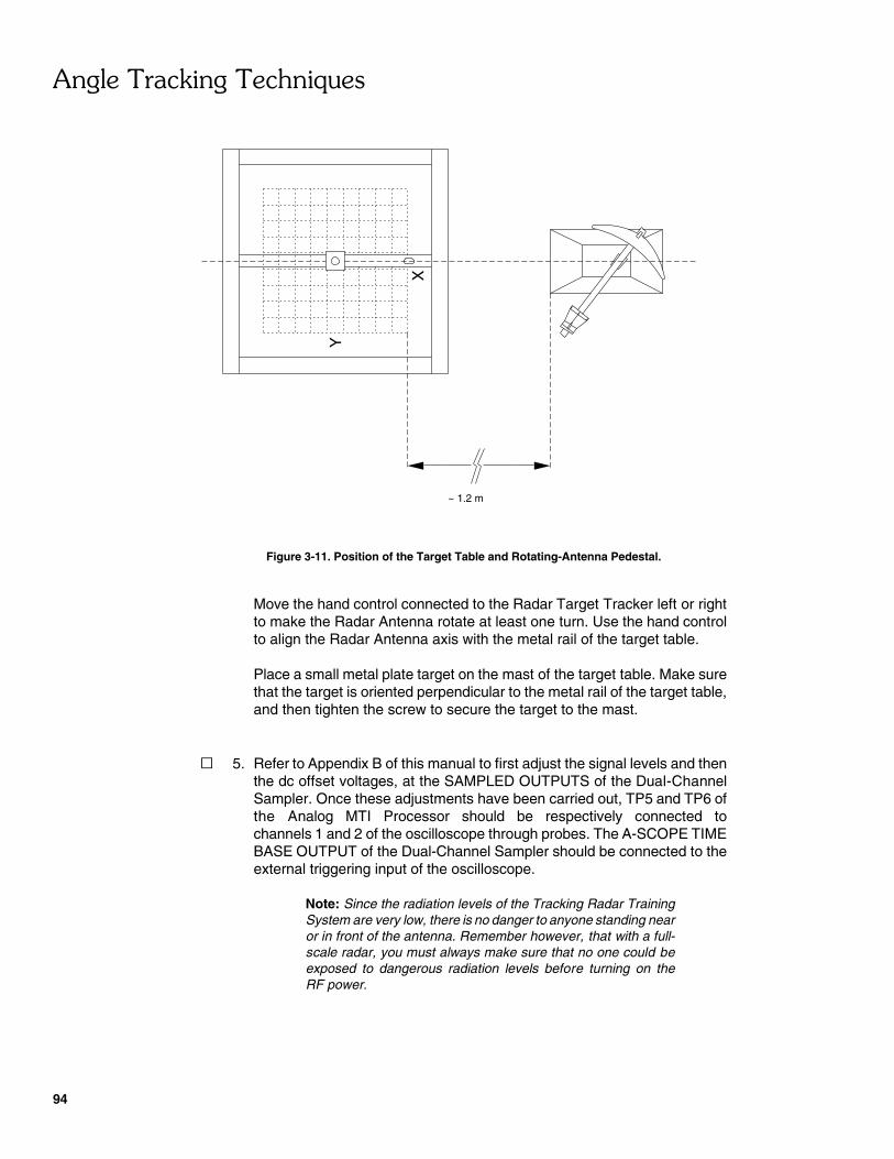
#$�������(�$����!�+���
94
~ 1.2 m
Y
X
Figure 3-11. Position of the Target Table and Rotating-Antenna Pedestal.
Move the hand control connected to the Radar Target Tracker left or rightto make the Radar Antenna rotate at least one turn. Use the hand controlto align the Radar Antenna axis with the metal rail of the target table.
Place a small metal plate target on the mast of the target table. Make surethat the target is oriented perpendicular to the metal rail of the target table,and then tighten the screw to secure the target to the mast.
� 5. Refer to Appendix B of this manual to first adjust the signal levels and thenthe dc offset voltages, at the SAMPLED OUTPUTS of the Dual-ChannelSampler. Once these adjustments have been carried out, TP5 and TP6 ofthe Analog MTI Processor should be respectively connected tochannels 1 and 2 of the oscilloscope through probes. The A-SCOPE TIMEBASE OUTPUT of the Dual-Channel Sampler should be connected to theexternal triggering input of the oscilloscope.
Note: Since the radiation levels of the Tracking Radar TrainingSystem are very low, there is no danger to anyone standing nearor in front of the antenna. Remember however, that with a full-scale radar, you must always make sure that no one could beexposed to dangerous radiation levels before turning on theRF power.

#$�������(�$����!�+���
95
Make the following adjustment on the Analog MTI Processor:
RANGE . . . . . . . . . . . . . . . . . . . . . . . . . . . . 3.6 m
� 6. Refer to Appendix B of this manual to calibrate the origin of the O-scopedisplay so that it corresponds as closely as possible to the location of theRadar Antenna horns (0 m).
Refer to Appendix B of this manual to adjust the bearing frictioncompensation circuit of the Radar Target Tracker (if necessary).
Lobe Switching
� 7. On the Radar Target Tracker, remove the cable which connects the LOBESWITCH CONTROL OUTPUT to the LOBE SWITCH CONTROL INPUT.
Connect the LOBE SWITCH CONTROL INPUT of the Radar TargetTracker to the +15-V dc output of the Power Supply using the BNC con-nector/banana plug cable provided with the tracking radar. This applies a+15-V dc bias voltage to the microwave switch of the Radar Antenna.
� 8. On the Radar Transmitter, depress the RF POWER push button. TheRF POWER ON LED should start to flash on and off. This indicates thatRF power is being radiated by the Radar Antenna.
Using the hand control, slightly vary the direction of the Radar Antenna sothat the amplitude of the target echo pulse on the O-scope display ismaximum.
Note: The target echo pulse on the O-scope display may beclipped due to saturation in the Radar Target Tracker.
Is the target located to the right or left of the Radar Antenna axis (whenlooking at the target from the antenna)?
Which horn of the antenna is used?
� 9. Using a small metal plate target, gradually block the aperture of theantenna horn which you think is not used. While doing this, observe thetarget echo pulse on the O-scope display.
#$�������(�$����!�+���
96
Describe what happens. Briefly explain.
Does this confirm the answer you gave in the previous step about theantenna horn that is used?
� Yes � No
� 10. On the Radar Transmitter, set the RF POWER switch to the STANDBYposition. The RF POWER STANDBY LED should be lit.
Disconnect the LOBE SWITCH CONTROL INPUT of the Radar TargetTracker from the +15-V dc output of the Power Supply then connect it tothe �15-V dc output of the same module. This applies a �15-V dc biasvoltage to the microwave switch of the Radar Antenna.
� 11. On the Radar Transmitter, depress the RF POWER push button. TheRF POWER ON LED should start to flash on and off.
Using the hand control, slightly vary the direction of the Radar Antenna sothat the echo pulse of the small metal plate target appears on the O-scopedisplay. Slightly readjust the direction of the Radar Antenna so that theamplitude of the target echo pulse is maximum.
Note: The target echo pulse on the O-scope display may beclipped due to saturation in the Radar Target Tracker.
Is the target located to the right or left of the Radar Antenna axis (whenlooking at the target from the antenna)?
Which horn of the antenna is used?
� 12. Using a small metal plate target, gradually block the aperture of theantenna horn which you think is not used. While doing this, observe thetarget echo pulse on the O-scope display.
#$�������(�$����!�+���
97
Describe what happens. Briefly explain.
Does this confirm the answer you gave in the previous step about theantenna horn that is used?
� Yes � No
Antenna Beam Patterns
� 13. On the Radar Transmitter, set the RF POWER switch to the STANDBYposition. The RF POWER STANDBY LED should be lit.
Remove the small metal plate target from the mast of the target table.
Place a large metal plate target on the mast of the target table. Make surethat the target is oriented perpendicular to the metal rail of the target table,and then tighten the screw to secure the target to the mast.
On the Target Controller, use the Y-axis position control to place the targetat the far end of the target table. The target range is now approximately2.0 m since the grid of the target table is approximately 1.1 m from thehorns of the Radar Antenna.
� 14. Using a probe, connect TP7 of the Radar Target Tracker (radar videosignal) to channel 1 of a second oscilloscope.
Connect the external triggering input of the second oscilloscope to OUT-PUT A (PRF OUTPUT) of the Radar Synchronizer.
Make the following settings on the second oscilloscope:
Channel 1 . . . . . . . . . . . . . . . . . . . . . . . 0.5 V/DIVVertical Mode . . . . . . . . . . . . . . . . . . . . . . . . CH-1Time Base . . . . . . . . . . . . . . . . . . . . . . 0.5 ms/DIVTrigger . . . . . . . . . . . . . . . . . . . . . . . . . . . . . . EXT.
On the Radar Transmitter, depress the RF POWER push button. TheRF POWER ON LED should start to flash on and off.
On the Analog MTI Processor, set the GAIN control so that the amplitudeof the target echo pulse at TP7 is approximately 3.0 V.
� 15. On the Antenna Controller, make sure the POSITION MODE push buttonis depressed.

#$�������(�$����!�+���
98
Manually rotate the Radar Antenna counterclockwise until the amplitude ofthe target echo pulse at TP7 decreases to approximately 0.3 V. Record inthe first row of Table 3-1 the azimuth of the Radar Antenna (indicated onthe Antenna Controller DISPLAY) and the amplitude of the target echopulse at TP7.
Manually rotate the Radar Antenna clockwise by steps of 1� so that theantenna beam (right lobe) scans the target. For each step, record inTable 3-1 the azimuth of the Radar Antenna and the amplitude of the targetecho pulse at TP7.
ANTENNAAZIMUTH
TARGETECHO AMPLITUDE
(RIGHT LOBE)
degrees V
Table 3-1. Target Echo Amplitude (at TP7) Versus Radar Antenna Azimuth (right lobe).
� 16. On the Radar Transmitter, set the RF POWER switch to the STANDBYposition. The RF POWER STANDBY LED should be lit.
Disconnect the LOBE SWITCH CONTROL INPUT of the Radar TargetTracker from the �15-V dc output of the Power Supply then connect it tothe +15-V dc output of the same module.
On the Radar Transmitter, depress the RF POWER push button. TheRF POWER ON LED should start to flash on and off and the target echopulse should appear at TP7.

#$�������(�$����!�+���
99
� 17. Manually rotate the Radar Antenna clockwise until the amplitude of thetarget echo pulse at TP7 decreases to approximately 0.3 V. Record in thefirst row of Table 3-2 the azimuth of the Radar Antenna and the amplitudeof the target echo pulse at TP7.
ANTENNAAZIMUTH
TARGETECHO AMPLITUDE
(LEFT LOBE)
degrees V
Table 3-2. Target Echo Amplitude (at TP7) Versus Radar Antenna Azimuth (left lobe).
Manually rotate the Radar Antenna counterclockwise by steps of 1� so thatthe antenna beam (left lobe) scans the target. For each step, record inTable 3-2 the azimuth of the Radar Antenna and the amplitude of the targetecho pulse at TP7.
� 18. On the Radar Transmitter, set the RF POWER switch to the STANDBYposition. The RF POWER STANDBY LED should be lit.
Use the data in Tables 3-1 and 3-2 to plot in Figure 3-12 the right and lefttwo-way beam patterns (right and left lobes) of the antenna.
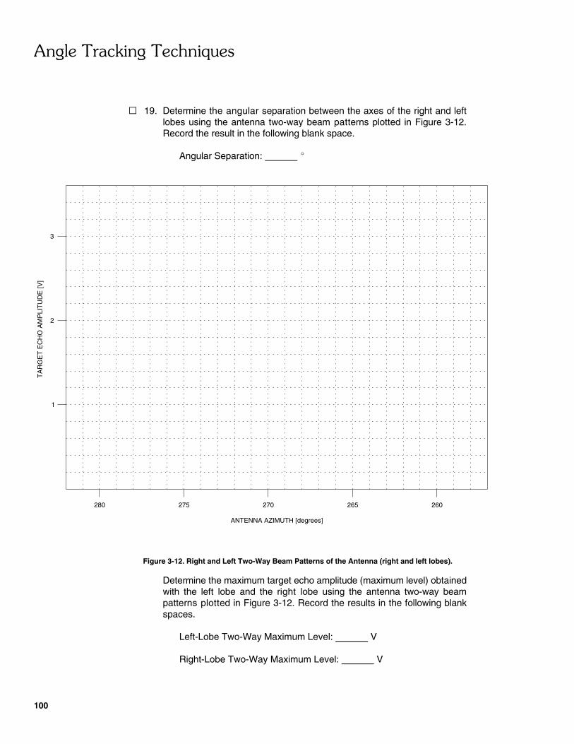
#$�������(�$����!�+���
100
3
2
1
TA
RG
ET
EC
HO
AM
PLI
TU
DE
[V]
ANTENNA AZIMUTH [degrees]
280 275 270 265 260
� 19. Determine the angular separation between the axes of the right and leftlobes using the antenna two-way beam patterns plotted in Figure 3-12.Record the result in the following blank space.
Angular Separation: �
Figure 3-12. Right and Left Two-Way Beam Patterns of the Antenna (right and left lobes).
Determine the maximum target echo amplitude (maximum level) obtainedwith the left lobe and the right lobe using the antenna two-way beampatterns plotted in Figure 3-12. Record the results in the following blankspaces.
Left-Lobe Two-Way Maximum Level: V
Right-Lobe Two-Way Maximum Level: V
#$�������(�$����!�+���
101
Calculate the mean value of the right- and left-lobe two-way maximumlevels to determine the two-way beam maximum level. Record the result inthe following blank space.
Two-Way Beam Maximum Level: V
Determine the target echo amplitude at the point the antenna two-waybeam patterns in Figure 3-12 intersect. This corresponds to the two-waybeam crossover level. Record the result in the following blank space.
Two-Way Beam Crossover Level: V
Calculate the crossover loss using the following equation:
Crossover Loss � 20 x log Two�Way Beam Crossover LevelTwo�Way Beam Maximum Level
� 20 x log � � � db
Lobe Switching Control
� 20. Remove the cable connecting the LOBE SWITCH CONTROL INPUT of theRadar Target Tracker to the +15-V dc output of the Power Supply.
On the Radar Target Tracker, install a BNC T-connector on the LOBESWITCH CONTROL OUTPUT then connect this output to the LOBESWITCH CONTROL INPUT of the same module and to channel 2 of thesecond oscilloscope.
Make the following settings on the second oscilloscope:
Channel 1 . . . . . . . . . . . . . . . . . . . . . . . . 1 V/DIVChannel 2 . . . . . . . . . . . . . . . . . . . . . . . . 5 V/DIVVertical Mode . . . . . . . . . . . . . . . . . . . . . . . CHOP.Time Base . . . . . . . . . . . . . . . . . . . . . . . 2 ms/DIVTrigger . . . . . . . . . . . . . . . . . . . . . . . . . . . . . CH-2
On the Target Controller, select the SPEED MODE then select thePOSITION MODE to place the target in the center of the target table grid.
Use the hand control to align the Radar Antenna axis with the target.
� 21. On the Radar Transmitter, depress the RF POWER push button. TheRF POWER ON LED should start to flash on and off and the target echopulse should appear at TP7.

#$�������(�$����!�+���
102
Manually rotate the Radar Antenna counterclockwise slightly so that thetarget is to the right of the antenna axis. Sketch the waveforms of the radarvideo signal and the LOBE SWITCH CONTROL OUTPUT signal inFigure 3-13.
Figure 3-13. Radar Video Signal and LOBE SWITCH CONTROL OUTPUT Signal (target to the rightof the antenna axis).
Why does the amplitude of the target echo pulse change from oneinterpulse period to the next?
Briefly explain why the amplitude of the target echo pulse obtained whenthe LOBE SWITCH CONTROL OUTPUT signal is negative is higher thanthat obtained when the LOBE SWITCH CONTROL OUTPUT signal ispositive.
� 22. Manually rotate the Radar Antenna clockwise slightly so that the target isto the left of the antenna axis. Sketch the waveforms of the radar videosignal and LOBE SWITCH CONTROL OUTPUT signal in Figure 3-14.

#$�������(�$����!�+���
103
Briefly explain why the amplitude of the target echo pulse obtained whenthe LOBE SWITCH CONTROL OUTPUT signal is positive is higher thanthat obtained when the LOBE SWITCH CONTROL OUTPUT signal isnegative.
Figure 3-14. Radar Video Signal and LOBE SWITCH CONTROL OUTPUT Signal (target to the left ofthe antenna axis).
� 23. On the Radar Target Tracker, set the LOBE CONTROL RATE push buttonto the PRF/4 position while observing the signals on the secondoscilloscope.
Sketch the waveforms of the radar video signal and LOBE SWITCHCONTROL OUTPUT signal in Figure 3-15.

#$�������(�$����!�+���
104
Figure 3-15. Radar Video Signal and LOBE SWITCH CONTROL OUTPUT Signal (target to the left ofthe antenna axis and lobe control rate set to PRF/4).
Describe what happens when the lobe control rate passes from PRF/2 toPRF/4.
� 24. On the Radar Transmitter, make sure that the RF POWER switch is in theSTANDBY position. The RF POWER STANDBY LED should be lit. Placeall POWER switches in the O (off) position and disconnect all cables andaccessories.
CONCLUSION
In this exercise, you learned that lobe switching alternately switches the antennabeam between two positions located on both sides of the antenna axis. Youobserved that when a +15-V dc voltage is applied to the LOBE SWITCH CONTROLINPUT of the Radar Target Tracker, the RF signal flows through the right horn ofthe Radar Antenna and the beam axis is to the left of the antenna axis. Conversely,when a �15-V dc voltage is applied to the LOBE SWITCH CONTROL INPUT, theRF signal flows through the left horn of the Radar Antenna and the beam axis is tothe right of the antenna axis. You saw that the antenna two-way beam patternsobtained in the two positions overlap. You observed that the signal level at the pointthe two patterns intersect (two-way beam crossover level) is less than the two-waybeam maximum level. You saw that in the Lab-Volt tracking radar, a bipolar square-wave signal is used to alternately switch the antenna beam between the twopositions.

#$�������(�$����!�+���
105
REVIEW QUESTIONS
1. Briefly explain how angle tracking is usually achieved in tracking radars.
2. Briefly explain the lobe-switching angle tracking technique.
3. What is the beam crossover level?
4. Briefly explain what is the crossover loss.
5. What advantage does the monopulse angle tracking technique have over thelobe switching and conical scan angle tracking techniques?


���������������
����
���������
#���'�����$����'������

109
�����������
������!��(�))���*����&)��������+���������������
EXERCISE OBJECTIVE
To demonstrate the effect of AM noise and repeater inverse gain jamming, twoangular deceptive EA used against sequential lobing radars. To outline the reasonswhy radar PRF agility is an effective EP against inverse gain jammers.
DISCUSSION
Introduction
As stated in this Unit's Discussion of Fundamentals, conical scan and sequentiallobing radars, unlike monopulse radars, are vulnerable to amplitude-modulatedjamming signals. These radars operate by moving their antenna beam to induce anamplitude modulation onto the target echo signal, this for the purpose of angulartracking. When the radar antenna is pointed directly towards the tracked target, theamplitude of the target echo signal is constant over time. Non-radar inducedamplitude variations onto the target echo signal, due to scintillation or a jammingsignal, are a cause of error and uncertainty in the target’s angular position as seenby the radar.
Inverse Gain Jamming
Inverse gain jamming, an angular DECM, consists in directing towards the radarantenna, either a false target signal (repeater inverse gain jamming) or a noisejamming signal (AM noise jamming) with an amplitude modulation in phaseopposition to that generated by the scanning (or lobing) radar beam.
The transmitted amplitude modulation can be implemented either as a direct inverseof the radar’s amplitude modulation, or as on-off modulation, whereby the "on"period is made to coincide with the interval when the radar-signal amplitude isminimum. Either of these types of amplitude modulations can cause an apparentangular error in the radar’s tracking system. This apparent tracking error is oppositein sign to the actual tracking error needed to correct for the radar antenna’s angularposition, as is illustrated in Figure 3-2 (a). In this figure, erroneous angular trackinginformation is introduced into the radar angle tracking loop, because the amplitudeof the target echo signal, received through one lobe, has been made greater by thepresence of the jamming signal.
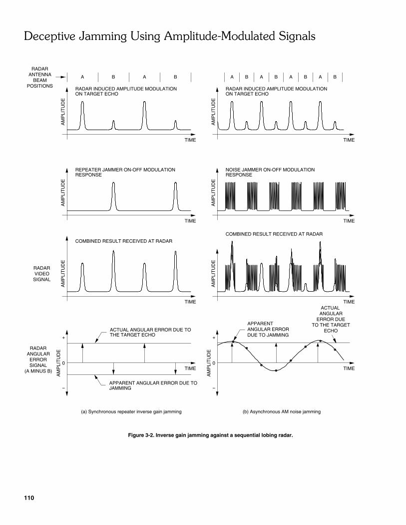
"������'��,����$�-��$�#��������)%�����������$���
110
AM
PLI
TU
DE
A B BA A B BA BA BA
AM
PLI
TU
DE
AM
PLI
TU
DE
RADAR INDUCED AMPLITUDE MODULATIONON TARGET ECHO
REPEATER JAMMER ON-OFF MODULATIONRESPONSE
RADAR INDUCED AMPLITUDE MODULATIONON TARGET ECHO
COMBINED RESULT RECEIVED AT RADAR
AM
PLI
TU
DE
AM
PLI
TU
DE
0
+
−
TIME TIME
TIME
TIME
TIME
ACTUAL ANGULAR ERROR DUE TOTHE TARGET ECHO
APPARENT ANGULAR ERROR DUE TOJAMMING
(a) Synchronous repeater inverse gain jamming
ANTENNABEAM
POSITIONS
RADAR
RADAR
SIGNALVIDEO
RADARANGULAR
ERRORSIGNAL
(A MINUS B)
AM
PLI
TU
DE
TIME
NOISE JAMMER ON-OFF MODULATIONRESPONSE
TIME
AM
PLI
TU
DE
TIME
+
0
AM
PLI
TU
DE
−
ANGULAR ERRORDUE TO JAMMING
APPARENT
(b) Asynchronous AM noise jamming
ACTUAL ANGULAR
ERROR DUETO THE TARGET
ECHO
COMBINED RESULT RECEIVED AT RADAR
Figure 3-2. Inverse gain jamming against a sequential lobing radar.
"������'��,����$�-��$�#��������)%�����������$���
111
Synchronicity
For inverse gain jamming to be effective, the frequency at which the jamming signalis amplitude modulated must be near the victim radar’s lobing (or scan) rate. Inversegain jamming is effective when the jamming signal is synchronized with the radarantenna’s lobing (or scan) rate. However, it can also be effective in anasynchronous (sweeping) mode which searches for the most suitable amplitudemodulation frequency that perturbs the radar angle tracking loop. Figure 3-2 (a)shows repeater inverse gain jamming synchronized to the radar lobing rate.Figure 3-2 (b) shows AM noise jamming transmitted asynchronously to the radarlobing rate.
When transmitted synchronously, the jammer’s amplitude modulation frequency isset equal to the radar's lobing (or scan) rate. This introduces a fixed angular errorinto the radar’s angle tracking loop, resulting, in an angular offset that deviates theradar antenna axis from the tracked target’s direction.
When transmitted asynchronously, the amplitude modulation frequency of thejamming signal may be slightly higher or lower than the radar's lobing (or scan) rate.This effectively creates a radar angular error signal with a beat frequency. The beatfrequency is equal to the difference between the amplitude modulation frequencyof the jamming signal and that induced onto the target echo signal by the radar(i.e. the radar lobing or scan rate). The jammer must set its amplitude modulationfrequency carefully so that the beat frequency is low enough to pass through theangular servomechanism’s bandwidth (typically in the range of a few Hertz).Otherwise, the effect of the received jamming signal is greatly attenuated by theangular tracking loop and, consequently, angular tracking is not, or barely, affected.
Inverse Gain Jamming with the Lab-Volt Radar Jamming Pod
The Radar Jamming Pod, as stated in Exercise 2-1, can on-off modulate either therepeater signal, or the noise jamming signal. Therefore, the Radar Jamming Podcan produce either repeater asynchronous inverse gain jamming, or asynchronousAM noise jamming. The on-off amplitude modulation frequency for these techniquescan be set close to the tracking radar's lobing rate. The modulation frequency ischanged using the Radar Jamming Pod remote controller.
Radar Electronic Protection Against Inverse Gain Jamming
Asynchronous and synchronous inverse gain jamming can be rendered ineffectiveagainst a conical scan or sequential lobing tracking radar by randomly changing ona pulse-to-pulse basis the radar’s pulse repetition frequency (PRF). Radars thathave this ability are said to have PRF agile emitters. PRF agility is a useful radarelectronic protection to inverse gain jamming. Patterned radar emitters, such asthose that can enable a staggered PRF, are only effective in reducing the amplitudeof the angular error caused by inverse gain jammers, they cannot eliminate theangular error completely. To completely eliminate the angular error, a PRF agileemitter is required. Unfortunately, truly PRF-agile radar emitters pose many designchallenges when implemented in pulsed Doppler radars. These radars require their
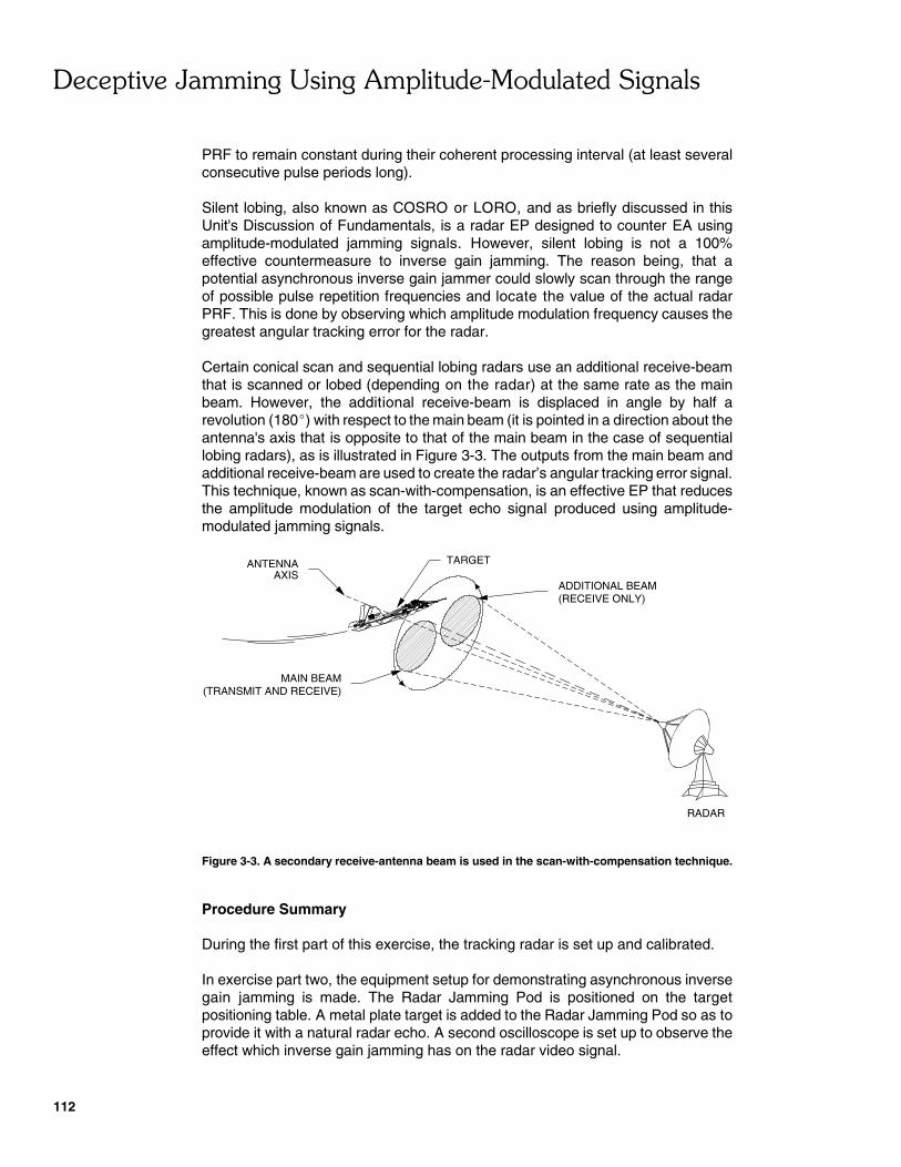
"������'��,����$�-��$�#��������)%�����������$���
112
RADAR
ADDITIONAL BEAM(RECEIVE ONLY)
(TRANSMIT AND RECEIVE)MAIN BEAM
ANTENNA TARGETAXIS
PRF to remain constant during their coherent processing interval (at least severalconsecutive pulse periods long).
Silent lobing, also known as COSRO or LORO, and as briefly discussed in thisUnit's Discussion of Fundamentals, is a radar EP designed to counter EA usingamplitude-modulated jamming signals. However, silent lobing is not a 100%effective countermeasure to inverse gain jamming. The reason being, that apotential asynchronous inverse gain jammer could slowly scan through the rangeof possible pulse repetition frequencies and locate the value of the actual radarPRF. This is done by observing which amplitude modulation frequency causes thegreatest angular tracking error for the radar.
Certain conical scan and sequential lobing radars use an additional receive-beamthat is scanned or lobed (depending on the radar) at the same rate as the mainbeam. However, the additional receive-beam is displaced in angle by half arevolution (180�) with respect to the main beam (it is pointed in a direction about theantenna's axis that is opposite to that of the main beam in the case of sequentiallobing radars), as is illustrated in Figure 3-3. The outputs from the main beam andadditional receive-beam are used to create the radar’s angular tracking error signal.This technique, known as scan-with-compensation, is an effective EP that reducesthe amplitude modulation of the target echo signal produced using amplitude-modulated jamming signals.
Figure 3-3. A secondary receive-antenna beam is used in the scan-with-compensation technique.
Procedure Summary
During the first part of this exercise, the tracking radar is set up and calibrated.
In exercise part two, the equipment setup for demonstrating asynchronous inversegain jamming is made. The Radar Jamming Pod is positioned on the targetpositioning table. A metal plate target is added to the Radar Jamming Pod so as toprovide it with a natural radar echo. A second oscilloscope is set up to observe theeffect which inverse gain jamming has on the radar video signal.
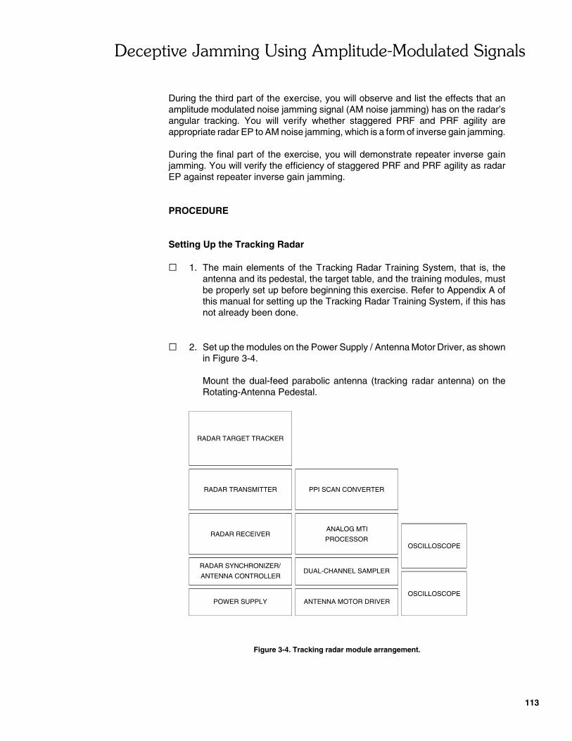
"������'��,����$�-��$�#��������)%�����������$���
113
RADAR SYNCHRONIZER/DUAL-CHANNEL SAMPLER
OSCILLOSCOPE
RADAR RECEIVER
PPI SCAN CONVERTERRADAR TRANSMITTER
RADAR TARGET TRACKER
ANTENNA CONTROLLER
ANTENNA MOTOR DRIVERPOWER SUPPLY
PROCESSOR
ANALOG MTI
OSCILLOSCOPE
During the third part of the exercise, you will observe and list the effects that anamplitude modulated noise jamming signal (AM noise jamming) has on the radar’sangular tracking. You will verify whether staggered PRF and PRF agility areappropriate radar EP to AM noise jamming, which is a form of inverse gain jamming.
During the final part of the exercise, you will demonstrate repeater inverse gainjamming. You will verify the efficiency of staggered PRF and PRF agility as radarEP against repeater inverse gain jamming.
PROCEDURE
Setting Up the Tracking Radar
� 1. The main elements of the Tracking Radar Training System, that is, theantenna and its pedestal, the target table, and the training modules, mustbe properly set up before beginning this exercise. Refer to Appendix A ofthis manual for setting up the Tracking Radar Training System, if this hasnot already been done.
� 2. Set up the modules on the Power Supply / Antenna Motor Driver, as shownin Figure 3-4.
Mount the dual-feed parabolic antenna (tracking radar antenna) on theRotating-Antenna Pedestal.
Figure 3-4. Tracking radar module arrangement.
"������'��,����$�-��$�#��������)%�����������$���
114
� 3. Make sure that on the Radar Transmitter, the RF POWER switch is in theSTANDBY position.
Make sure that on the Antenna Controller, the MANual ANTENNAROTATION MODE push button is depressed and that the SPEED controlis in the 0 position.
Set the Power Supply POWER switch to the I (on) position. Do the samefor the other radar modules that have a POWER switch.
� 4. Figure 3-5 shows the block diagram of the tracking radar including theconnections to the PPI Scan Converter.
Install a BNC T-connector on OUTPUT B of the Radar Synchronizer thenconnect the modules as shown in the block diagram.
Note: The SYNC. TRIGGER INPUT of the Dual-ChannelSampler and the PULSE GENERATOR TRIGGER INPUT of theRadar Transmitter must be connected directly to OUTPUT B ofthe Radar Synchronizer without passing through BNC T-connec-tors.
� 5. Calibrate and adjust the Tracking Radar Training System using ProceduresI to V of Appendix B of this manual.
� 6. Make the following adjustments to the tracking radar:
Operating Frequency . . . . . . . . . . . . . . . . . . . . . . . . . . . . 9.0 GHzPulse-Repetition Frequency . . . . . . . . . . . . . . . . . . . single, 288 HzPulse Width . . . . . . . . . . . . . . . . . . . . . . . . . . . . . . . . . . . . . . 1 nsObservation Range . . . . . . . . . . . . . . . . . . . . . . . . . . . . . . . 3.6 m
Turn the Radar Transmitter RF POWER on.
Inverse Gain Jamming Set-Up
� 7. Remove the small metal plate target, used for tracking radar calibration,from the target table mast.
Move the metal rail to one of either ends of the target table, it will not beused during this exercise.
Place the Radar Jamming Pod support, provided with the ConnectionLeads and Accessories, onto the target table. Position it such that it is inthe center of the target table grid.
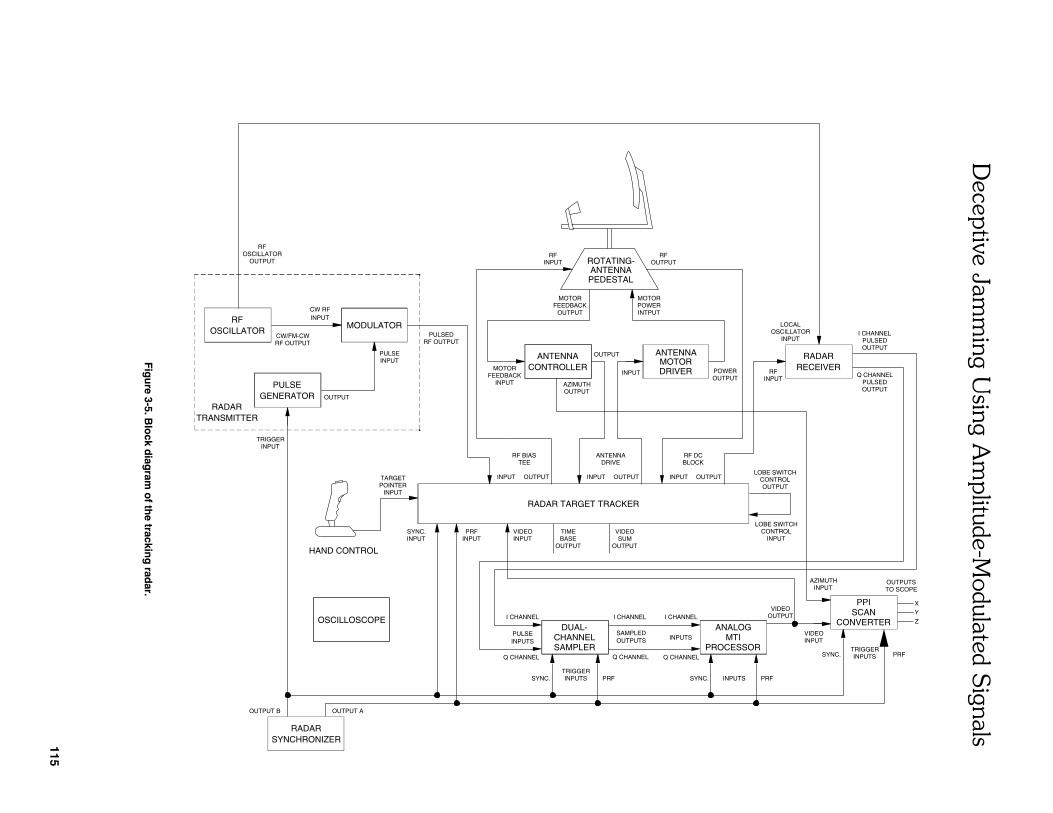
"���
���'�
�,����$�-
��$�#
������
��)%
�����������$���
115
RADAR TARGET TRACKER
SYNC.INPUT
PRFINPUT INPUT
VIDEO TIMEBASE
OUTPUT OUTPUTSUM
VIDEO
INPUTPOINTERTARGET
LOBE SWITCHCONTROLOUTPUT
LOBE SWITCHCONTROL
INPUT
INPUT OUTPUT
TEERF BIAS
DRIVEANTENNA
OUTPUTINPUT
BLOCKRF DC
OUTPUTINPUT
ANTENNACONTROLLER
ANTENNAMOTORDRIVER
AZIMUTHOUTPUT
OUTPUT
INPUT POWEROUTPUT
RECEIVERRADAR
RFINPUT
LOCALOSCILLATOR
INPUT
Q CHANNELPULSEDOUTPUT
OUTPUTPULSED
I CHANNEL
ROTATING-ANTENNAPEDESTAL
FEEDBACKMOTOR
INPUT
FEEDBACKMOTOR
OUTPUT INTPUTPOWERMOTOR
CHANNELDUAL-
INPUTS
INPUTSTRIGGER
Q CHANNELSAMPLER
PULSE
I CHANNEL
Q CHANNEL
SYNC. PRF
SAMPLEDOUTPUTS
I CHANNEL
SYNC.
Q CHANNEL
I CHANNEL
INPUTS MTIPROCESSOR
INPUTS PRF
ANALOGOUTPUTVIDEO
CONVERTER
PPISCAN
PRFTRIGGERINPUTSSYNC.
INPUTAZIMUTH OUTPUTS
TO SCOPE
X
Y
Z
RADARSYNCHRONIZER
OSCILLOSCOPE
HAND CONTROL
OUTPUT B OUTPUT A
INPUTRF
OUTPUTRF
RFOSCILLATOR
CW/FM-CWRF OUTPUT
INPUTMODULATOR
PULSEDRF OUTPUT
CW RF
GENERATORPULSE
OUTPUTOSCILLATOR
RF
TRIGGERINPUT
TRANSMITTERRADAR
INPUTPULSE
OUTPUT
INPUTVIDEO
Fig
ure 3-5. B
lock d
iagram
of th
e tracking
radar.
"������'��,����$�-��$�#��������)%�����������$���
116
� 8. Make sure that a 50-� load is connected to the Radar Jamming PodCOMPLEMENTARY RF OUTPUT.
Install the Radar Jamming Pod onto its support (in the horizontal position),using the short support shaft.
Align the Radar Jamming Pod horn antennas with the shaft of the Rotating-Antenna Pedestal.
Rotate the Radar Jamming Pod infrared receiver towards the direction fromwhere you will be using the remote controller.
� 9. Turn the Radar Jamming Pod on.
Note that the Radar Jamming Pod status indicates that the Repeater is on.Adjust the remote controller settings to match the Radar Jamming Podstatus (the Repeater is on, all else is off).
� 10. Make sure the radar antenna axis is aligned with the Radar Jamming Pod.This can be done by observing the O-scope display while adjusting theradar antenna bearing in an attempt to equalize the repeated echo signalamplitudes of the left and right lobes.
Observing the O-scope display, set the Analog MTI Processor GAIN controlso that the amplitude of the repeated echo signal is approximately 2.0 V.
Note the range of the repeated echo signal as read-off from the O-scopedisplay.
� 11. Using the remote controller, turn the Radar Jamming Pod Repeater off.
� 12. Retract the Radar Jamming Pod target positioning arm and place at its tipthe large (20x20 cm) metal plate target. Adjust the orientation of the metalplate target so as to maximize its echo signal on the O-scope display, whiletrying to have approximately the same amplitude in both the right and leftlobes.
Using the positioning arm while observing the O-scope display, adjust thedistance of the large metal plate target so that the range of its echo signalmatches the range of the repeated echo signal that you noted previously.
Note: If, after adjusting the distance of the large metal platetarget, the echo signal amplitude is not the same in the left andright lobes, slightly readjust the target orientation.
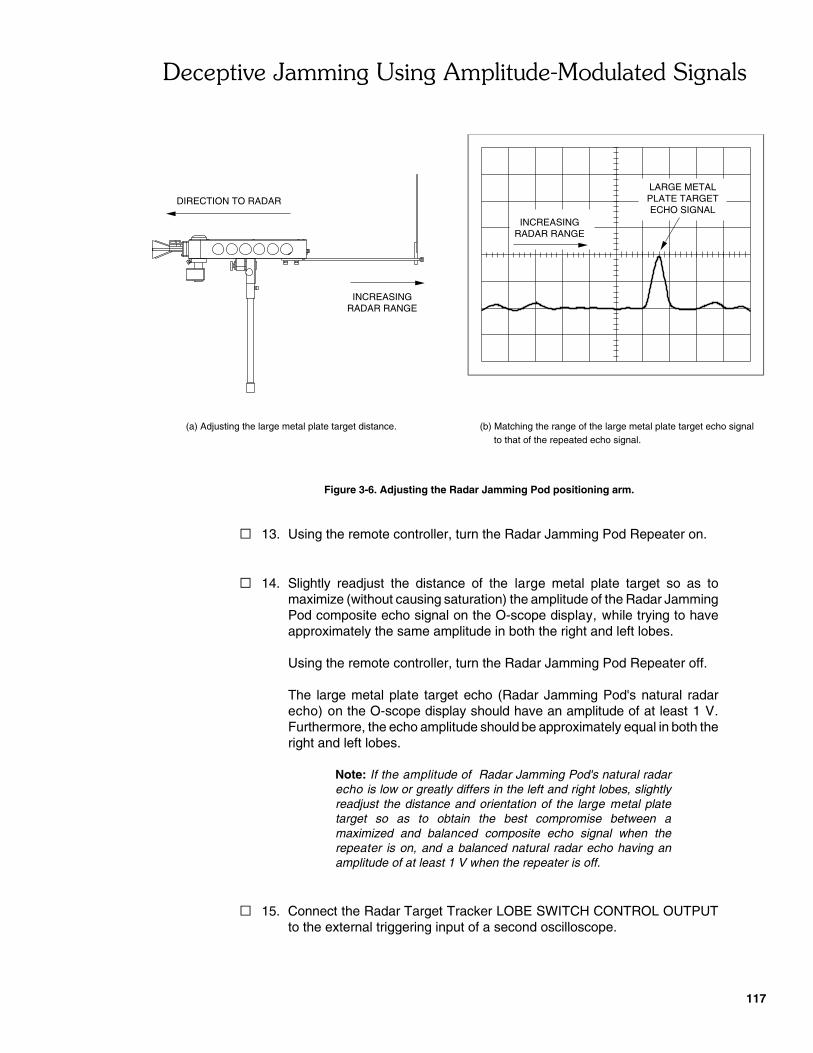
"������'��,����$�-��$�#��������)%�����������$���
117
DIRECTION TO RADAR
INCREASINGRADAR RANGE
(a) Adjusting the large metal plate target distance.
RADAR RANGEINCREASING
LARGE METALPLATE TARGETECHO SIGNAL
(b) Matching the range of the large metal plate target echo signalto that of the repeated echo signal.
Figure 3-6. Adjusting the Radar Jamming Pod positioning arm.
� 13. Using the remote controller, turn the Radar Jamming Pod Repeater on.
� 14. Slightly readjust the distance of the large metal plate target so as tomaximize (without causing saturation) the amplitude of the Radar JammingPod composite echo signal on the O-scope display, while trying to haveapproximately the same amplitude in both the right and left lobes.
Using the remote controller, turn the Radar Jamming Pod Repeater off.
The large metal plate target echo (Radar Jamming Pod's natural radarecho) on the O-scope display should have an amplitude of at least 1 V.Furthermore, the echo amplitude should be approximately equal in both theright and left lobes.
Note: If the amplitude of Radar Jamming Pod's natural radarecho is low or greatly differs in the left and right lobes, slightlyreadjust the distance and orientation of the large metal platetarget so as to obtain the best compromise between amaximized and balanced composite echo signal when therepeater is on, and a balanced natural radar echo having anamplitude of at least 1 V when the repeater is off.
� 15. Connect the Radar Target Tracker LOBE SWITCH CONTROL OUTPUTto the external triggering input of a second oscilloscope.
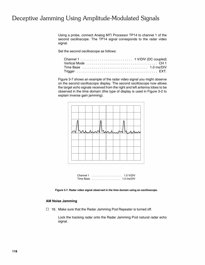
"������'��,����$�-��$�#��������)%�����������$���
118
Using a probe, connect Analog MTI Processor TP14 to channel 1 of thesecond oscilloscope. The TP14 signal corresponds to the radar videosignal.
Set the second oscilloscope as follows:
Channel 1 . . . . . . . . . . . . . . . . . . . . . . . . . . . 1 V/DIV (DC coupled)Vertical Mode . . . . . . . . . . . . . . . . . . . . . . . . . . . . . . . . . . . . . CH 1Time Base . . . . . . . . . . . . . . . . . . . . . . . . . . . . . . . . . . 1.0 ms/DIVTrigger . . . . . . . . . . . . . . . . . . . . . . . . . . . . . . . . . . . . . . . . . . EXT.
Figure 3-7 shows an example of the radar video signal you might observeon the second oscilloscope display. The second oscilloscope now allowsthe target echo signals received from the right and left antenna lobes to beobserved in the time domain (this type of display is used in Figure 3-2 toexplain inverse gain jamming).
Channel 1 . . . . . . . . . . . . . . . . . . . . . 1.0 V/DIVTime Base . . . . . . . . . . . . . . . . . . . . 1.0 ms/DIV
Figure 3-7. Radar video signal observed in the time domain using an oscilloscope.
AM Noise Jamming
� 16. Make sure that the Radar Jamming Pod Repeater is turned off.
Lock the tracking radar onto the Radar Jamming Pod natural radar echosignal.
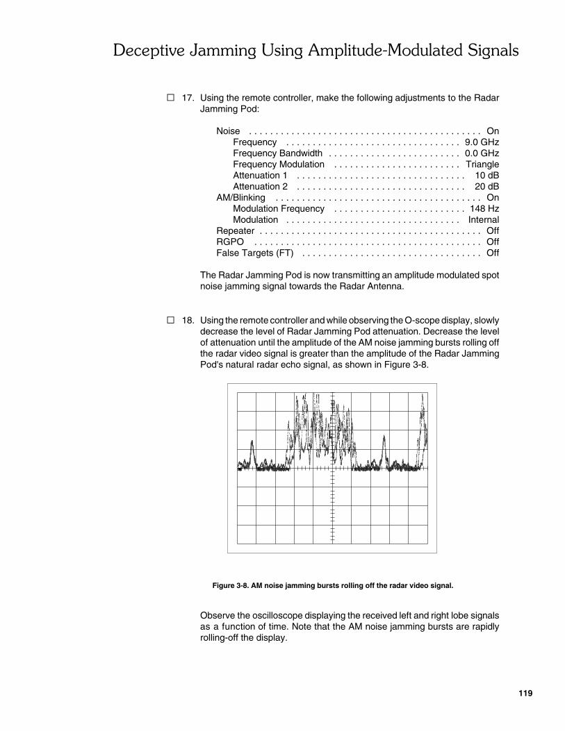
"������'��,����$�-��$�#��������)%�����������$���
119
� 17. Using the remote controller, make the following adjustments to the RadarJamming Pod:
Noise . . . . . . . . . . . . . . . . . . . . . . . . . . . . . . . . . . . . . . . . . . . . OnFrequency . . . . . . . . . . . . . . . . . . . . . . . . . . . . . . . . . 9.0 GHzFrequency Bandwidth . . . . . . . . . . . . . . . . . . . . . . . . . 0.0 GHzFrequency Modulation . . . . . . . . . . . . . . . . . . . . . . . . TriangleAttenuation 1 . . . . . . . . . . . . . . . . . . . . . . . . . . . . . . . . 10 dBAttenuation 2 . . . . . . . . . . . . . . . . . . . . . . . . . . . . . . . . 20 dB
AM/Blinking . . . . . . . . . . . . . . . . . . . . . . . . . . . . . . . . . . . . . . . OnModulation Frequency . . . . . . . . . . . . . . . . . . . . . . . . . 148 HzModulation . . . . . . . . . . . . . . . . . . . . . . . . . . . . . . . . . Internal
Repeater . . . . . . . . . . . . . . . . . . . . . . . . . . . . . . . . . . . . . . . . . . OffRGPO . . . . . . . . . . . . . . . . . . . . . . . . . . . . . . . . . . . . . . . . . . . OffFalse Targets (FT) . . . . . . . . . . . . . . . . . . . . . . . . . . . . . . . . . . Off
The Radar Jamming Pod is now transmitting an amplitude modulated spotnoise jamming signal towards the Radar Antenna.
� 18. Using the remote controller and while observing the O-scope display, slowlydecrease the level of Radar Jamming Pod attenuation. Decrease the levelof attenuation until the amplitude of the AM noise jamming bursts rolling offthe radar video signal is greater than the amplitude of the Radar JammingPod's natural radar echo signal, as shown in Figure 3-8.
Figure 3-8. AM noise jamming bursts rolling off the radar video signal.
Observe the oscilloscope displaying the received left and right lobe signalsas a function of time. Note that the AM noise jamming bursts are rapidlyrolling-off the display.

"������'��,����$�-��$�#��������)%�����������$���
120
Does the AM noise jamming have a significant effect on the angulartracking? Briefly explain why.
� 19. Using the remote controller, decrease in 1-Hz steps the amplitudemodulation frequency of the Radar Jamming Pod signal until it is equal tothe radar lobing rate (144 Hz). While decreasing the amplitude modulationfrequency, observe the effects of the AM noise jamming on: 1) the roll-offrate of the noise bursts displayed on the second oscilloscope, and 2) theradar antenna’s angular tracking.
Note: If the target tracking lock is lost while performing this step,slightly increase the Radar Jamming Pod attenuation levelby 1 dB and lock the tracking radar, once again, onto the RadarJamming Pod's echo signal.
Briefly explain the relation between the roll-off rate of the noise bursts in theradar video signal, and the noise jamming amplitude modulation frequency.
Briefly explain how the rate and the amplitude of the antenna oscillationsvary with the amplitude modulation frequency of the noise jamming signal.
� 20. Using the remote controller, adjust the Radar Jamming Pod amplitudemodulation frequency to 143 Hz.
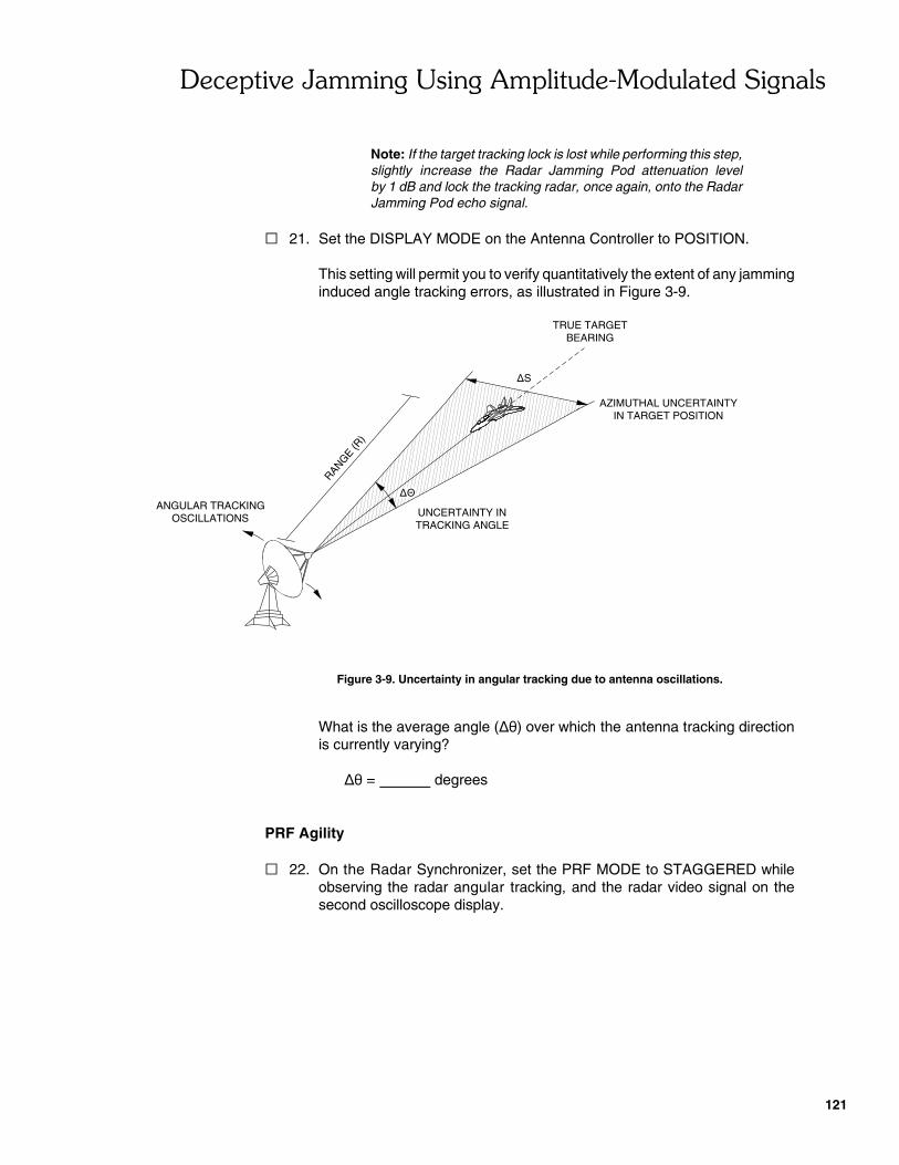
"������'��,����$�-��$�#��������)%�����������$���
121
þÞ
þS
RANGE (R
)
TRUE TARGETBEARING
IN TARGET POSITIONAZIMUTHAL UNCERTAINTY
UNCERTAINTY INTRACKING ANGLE
OSCILLATIONSANGULAR TRACKING
Note: If the target tracking lock is lost while performing this step,slightly increase the Radar Jamming Pod attenuation levelby 1 dB and lock the tracking radar, once again, onto the RadarJamming Pod echo signal.
� 21. Set the DISPLAY MODE on the Antenna Controller to POSITION.
This setting will permit you to verify quantitatively the extent of any jamminginduced angle tracking errors, as illustrated in Figure 3-9.
Figure 3-9. Uncertainty in angular tracking due to antenna oscillations.
What is the average angle (��) over which the antenna tracking directionis currently varying?
�� = degrees
PRF Agility
� 22. On the Radar Synchronizer, set the PRF MODE to STAGGERED whileobserving the radar angular tracking, and the radar video signal on thesecond oscilloscope display.
"������'��,����$�-��$�#��������)%�����������$���
122
Is staggered PRF an effective EP to AM noise jamming, a form of inversegain jamming? Briefly explain why.
� 23. On the Radar Synchronizer, set the PRF MODE back to SINGLE.
Change the tracking radar lobing rate to 108 Hz, by setting the RadarSynchronizer pulse repetition frequency (PRF) to 216 Hz. While doing this,observe the radar angular tracking, and the radar video signal on thesecond oscilloscope display.
Describe the effect that changing the tracking radar lobing rate had on thejamming induced antenna oscillations. Briefly explain why.
� 24. Using the remote controller, make the following adjustments to the RadarJamming Pod:
Noise . . . . . . . . . . . . . . . . . . . . . . . . . . . . . . . . . . . . . . . . . . . . OffAM/Blinking . . . . . . . . . . . . . . . . . . . . . . . . . . . . . . . . . . . . . . . OffRepeater . . . . . . . . . . . . . . . . . . . . . . . . . . . . . . . . . . . . . . . . . OffRGPO . . . . . . . . . . . . . . . . . . . . . . . . . . . . . . . . . . . . . . . . . . . OffFalse Targets (FT) . . . . . . . . . . . . . . . . . . . . . . . . . . . . . . . . . . Off
The Radar Jamming Pod is no longer transmitting an amplitude modulatedspot noise jamming signal towards the Radar Antenna.
Repeater Inverse Gain Jamming
� 25. Make the following settings to the tracking radar:
Pulse-Repetition Frequency . . . . . . . . . . . . . . . . . . . single, 288 Hz
Make certain that the tracking radar is locked onto the Radar Jamming Podnatural radar echo signal.
"������'��,����$�-��$�#��������)%�����������$���
123
� 26. Using the remote controller, enable the Radar Jamming Pod Repeater.
� 27. Using the remote controller, begin to amplitude (on-off) modulate therepeated echo signal, by making the following adjustments to the RadarJamming Pod:
Noise . . . . . . . . . . . . . . . . . . . . . . . . . . . . . . . . . . . . . . . . . . . . OffAM/Blinking . . . . . . . . . . . . . . . . . . . . . . . . . . . . . . . . . . . . . . . On
Modulation Frequency . . . . . . . . . . . . . . . . . . . . . . . . . 148 HzModulation . . . . . . . . . . . . . . . . . . . . . . . . . . . . . . . . . Internal
Repeater . . . . . . . . . . . . . . . . . . . . . . . . . . . . . . . . . . . . . . . . . . OnRGPO . . . . . . . . . . . . . . . . . . . . . . . . . . . . . . . . . . . . . . . . . . . OffFalse Targets (FT) . . . . . . . . . . . . . . . . . . . . . . . . . . . . . . . . . . Off
Note that the difference between the amplitude modulation frequency of therepeated echo signal, and the radar’s lobing rate is too great to causesignificant angle-tracking errors.
� 28. Using the remote controller, decrease in 1-Hz steps the amplitudemodulation frequency of the Radar Jamming Pod repeated echo signal untilit is equal to the radar lobing rate (144 Hz). While decreasing the amplitudemodulation frequency, observe the effects of the repeater inverse gainjamming on: 1) the rate at which the right- and left-lobe target echo signals(displayed on the second oscilloscope) are amplitude modulated, and 2) theradar antenna’s angular tracking.
Briefly explain the relation between the rate at which the right- and left-lobetarget echo signals are amplitude modulated, and the amplitude modulationfrequency of the repeated echo signal.
Briefly explain how the rate and the amplitude of the antenna oscillationsvary with the amplitude modulation frequency of the repeated echo signal.
� 29. Using the remote controller, adjust the Radar Jamming Pod amplitudemodulation frequency to 145 Hz.
"������'��,����$�-��$�#��������)%�����������$���
124
� 30. On the Radar Synchronizer, set the PRF MODE to STAGGERED whileobserving the radar angular tracking, and the radar video signal on thesecond oscilloscope display.
Is staggered PRF an effective EP to repeater inverse gain jamming?
� Yes � No
� 31. On the Radar Synchronizer, set the PRF MODE back to SINGLE.
Change the tracking radar lobing rate to 108 Hz, by setting the RadarSynchronizer pulse repetition frequency (PRF) to 216 Hz. While doing this,observe the radar angular tracking, and the radar video signal on thesecond oscilloscope display.
Is PRF agility an effective EP to repeater inverse gain jamming?
� Yes � No
� 32. Turn off the tracking radar and the Radar Jamming Pod. Disconnect allcables and remove all accessories.
CONCLUSION
In this exercise, you demonstrated the effects of asynchronous inverse gainjamming against a tracking radar, by separately using, an amplitude-modulatednoise jamming signal, and an amplitude-modulated repeated echo signal. Youlearned that asynchronous inverse gain jamming can either introduce a deflectionin the radar antenna’s angular tracking, or cause the antenna to oscillate about thetracked target’s direction. While implementing this angle deception EA techniqueagainst the tracking radar, you were able to verify the effectiveness of PRF agility,and of staggered PRF as radar EP to AM noise jamming as well as repeater inversegain jamming.
REVIEW QUESTIONS
1. Briefly describe how inverse gain jamming affects the angle tracking loop of asequential lobing radar.

"������'��,����$�-��$�#��������)%�����������$���
125
2. Figure 3-3 graphically shows how in certain conical scan radars the scan-with-compensation technique is implemented. What is the purpose of the additionalreceive beam?
3. What is the difference between synchronous and asynchronous inverse gainjamming?
4. Inverse gain jamming against a sequential lobing radar, can be achieved by arepeater jammer in the following manner. The weaker radar signals received atthe jammer, before being repeated back to the radar, are amplified. Thestronger signals, before being repeated back to the radar, are attenuated.Briefly explain if this implementation of inverse gain jamming is donesynchronously or asynchronously with respect to the radar lobing rate.
5. Asynchronous and synchronous inverse gain jamming, can be renderedineffective against a sequential lobing tracking radar by randomly changing theradar’s pulse repetition frequency (PRF) on a pulse-to-pulse basis. Brieflyexplain why this electronic protection is effective.


���������������
����
�!���!�����#��� �#���

129
�����������
,������������-�.�����������&�/���)���
EXERCISE OBJECTIVE
When you have completed this exercise, you will be able to set up and operate thePhased Array Antenna with the Lab-Volt Digital Radar Training System.
DISCUSSION
The Digital MTD/PPI Processor is designed for the study of the digital signalprocessing techniques used in modern airport surveillance radars. The role of thedigital signal processing is to enhance the detection and tracking of moving targets.All echoes received by the radar are presented on a PPI display as green luminousspots, called blips, of various shapes and sizes. A cursor and various information,such as the system PRF, the observation range, the antenna rotation speed, thecursor position, etc., appear on the Monitor along with the PPI display. The positionof the cursor is controlled using a Keyboard and/or a Trackball.
Procedure Summary
First, you will set up the Lab-Volt Digital Radar Training System. Then you will makethe necessary settings in order to see the target reflections on the Monitor clearly.Using the target controller and the target table, you will set the targets in motion.Finally, using the Phased Array Antenna Controller, you will vary the scan speedand observe results on the Monitor.
PROCEDURE
Setting up the training system
� 1. Refer to Appendix B to set up the digital radar. Place the Phased ArrayAntenna as shown in Figure 1-1.
Note: DO NOT connect the power cable to the MOTOR POWERINPUT of the Rotating-Antenna Pedestal.
Operation and adjustments
� 2. Place 2 semi-circular cross section targets on the 2 masts located at bothends of the target holder as shown in Figure 1-1, and make sure Dy is closeto 2 m.
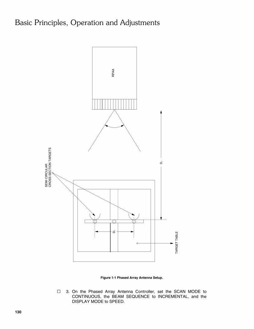
.��������������/�������������#�0�������
130
SE
MI C
IRC
ULA
RC
RO
SS
SE
CT
ION
TA
RG
ET
S
RP
AA
TA
RG
ET
TA
BLE
Dy
Dx
Figure 1-1 Phased Array Antenna Setup.
� 3. On the Phased Array Antenna Controller, set the SCAN MODE toCONTINUOUS, the BEAM SEQUENCE to INCREMENTAL, and theDISPLAY MODE to SPEED.
.��������������/�������������#�0�������
131
� 4. On the Phased Array Antenna Controller, set the scan speed to25 scan/min using the POSITION/SPEED (+) and (�) buttons.
� 5. Set the Q- and I-Channel DC Offset control knobs of the Dual-ChannelSampler and the GAIN control knobs of the Digital MTD / PPI Processor inorder to obtain the best picture possible on the Monitor. To do so, refer toAPPENDIX B.
� 6. Turn the Target Positioning System on by setting the POWER switchlocated on the target table to the I position (on). Select the TRAJECTORYmode by pressing the MODE selector button of the target controller untilthe TRAJECTORY mode LED lights up. Then, select the CIRCULARtrajectory by pressing the TRAJECTORY selector button until theTRAJECTORY display indicates the CIRCULAR trajectory. You can adjustthe target speed by turning TRAJECTORY SPEED control knob clockwiseto increase the speed and counterclockwise to decrease the speed.
� 7. On the Radar Transmitter, turn the RF POWER on. On the Dual-ChannelSampler, make sure that the 1.8 m span is selected and adjust the originby turning the ORIGIN control knob. You will know that the origin is setwhen the echoes clear up around the center of the screen.
� 8. On the Phased Array Antenna Controller, gradually increase the scanspeed by pressing the POSITION/SPEED (+) button while watching theMonitor. The radar image refresh rate should increase as the scan speedis increased. Note that as the scan speed is increased, target movementsdisplayed on the Monitor.
CONCLUSION
In this exercise, you set up the Lab-Volt Digital Radar Training System, you learnedthe operation of the Phased Array Antenna Controller. You also observed the effectof the scan speed on the PPI display.
REVIEW QUESTIONS
1. In a radar, what are the advantages of the digital signal processing?

.��������������/�������������#�0�������
132
2. What information appears on the Monitor?
3. What is the effect of increasing the scan speed?

��!����������
����
�������������������� ����


135
-�������
Note: Always read all of the choices in the question before selecting youranswer.
1. In pulsed radar, the usual waveform of the transmitted radar signal is
a. a pulsed sine wave.b. a continuous sine wave.c. a triangle wave.d. none of the above.
2. The position transducer in an antenna driving system
a. sends a signal from the antenna to the rest of the radar system.b. indicates the direction the antenna is pointing.c. is required to correctly display targets according to their directions.d. all of the above.
3. The antenna driving system may keep the antenna speed proportional to thePRF
a. by automatically adjusting the PRF according to the measuredinstantaneous antenna speed.
b. using a servo system to maintain the antenna speed constant.c. by alternating the direction of antenna movement.d. either a or b.
4. The rotary joint in an antenna system
a. couples the microwaves between the rotating antenna and the fixedwaveguide or cable.
b. prevents the transmitted signal from passing directly to the receiver.c. facilitates maintenance of the radar antenna.d. all of the above.
5. The bearing of a target
a. is the vertical direction of the target, expressed as an angle in the verticalplane from a reference direction.
b. is the horizontal direction of the target, expressed as an angle in thehorizontal plane from a reference direction.
c. determines the strength of the echo signal.d. depends on the reflecting characteristics of the target.
6. The target range is represented on the PPI display
a. by the distance of the blip from the origin.b. by the angle of the blip from a reference angle on the screen. c. by the brightness of the blip.d. by the color of the blip.

-�������� ������
136
7. The target bearing is represented on the PPI display
a. by the distance of the blip from the origin.b. by the angle of the blip from a reference angle on the screen.c. by the brightness of the blip.d. by the color of the blip.
8. The range rings on a PPI display
a. are rings whose radius can be continuously varied using controls on thedisplay.
b. are centered about the target of interest on the PPI display.c. are fixed, concentric rings placed at regular ranges on the display.d. none of the above.
9. The gain of the radar receiver
a. does not affect the resolution of the PPI display.b. affects only the range resolution on the PPI display.c. affects only the angular resolution on the PPI display.d. must be adjusted for optimum range and angular resolution on the PPI
display.
10. The digital scan converter
a. produces a conventional radial-sweep PPI display on a phosphorous screenwhich is then scanned in a raster-scan format.
b. produces a conventional radial-sweep PPI display on a computer memorywhich is then scanned in a raster-scan format.
c. is seldom used in modern radar systems.d. produces a digital A-scope display.

������������1����
��������������

�������������������� �����
139
UNIT 2 A PULSED RADAR SYSTEM
INTRODUCTORY INFORMATION
This unit explains in detail the operation of a pulsed radar system including aPPI display. Most explanations start from pulsed radar principles, and relate theseto the block diagrams of the circuitry commonly found in pulsed radars. In certaincases, the circuitry used in the Radar Training System is considered as an example.
Exercise 2-1 shows the operating principles of the radar transmitter and receiver.Various transmitter and receiver configurations, including those of the RadarTraining System, are discussed to illustrate the differences between them. Since theRadar Training System operates in the X-frequency band, and can produce pulsesas short as 1 ns, it is not possible to observe the pulsed RF signal using regularlaboratory classroom equipment. However, the modulating pulse signal in the RadarTransmitter and the demodulated pulse signals in the Radar Receiver are observedin this exercise using the Dual-Channel Sampler.
The antenna driving system is studied in detail in Exercise 2-2. The various possiblemovements of the antenna, the mechanical aspects of the system, and the controlcircuitry are some of the topics discussed. Note that the main purpose of thisexercise is to give students the basic knowledge necessary to understand how thePPI display is generated.
The first three parts of the exercise Procedure deal with the various antenna rotationmodes and with the monitoring of the antenna position and speed in the RadarTraining System. The fourth part studies the operation of the control amplifier usedin the feedback loop of the Radar Antenna driving system. This part is optional sincenot all radar systems use a feedback loop to control the rotation of the antenna.Familiarity with the operation of some simple electronic devices, such ascomparators, oscillators and choppers, as well as with some simple concepts suchas the amplitude, polarity or dc value of a signal is required to carry out this part ofthe exercise.
Exercise 2-3 explains the role and the generation of the PPI display. The use ofmarkers, such as the range rings, the VRM, and the EBL, to determine targetpositions is also covered. A brief review of the range and angular resolutions of apulsed radar is carried out since these are measured in this exercise using thePPI display.
Students will learn how to adjust the DC OFFSET controls on the Dual-ChannelSampler to eliminate any dc offsets in the I- and Q-channels of the Analog MTIProcessor. This is necessary to ensure that signals are properly detected by thethreshold detector in the PPI Scan Converter, since a dc offset alters the effectivethreshold level. They also learn how to calibrate the origin of the PPI display so thatthe PPI display correctly indicates target ranges. Then they will use the VRM andthe EBL of the PPI display to determine the positions of various metallic objects inthe laboratory classroom. The adjustment of the dc offsets and the origin calibrationof the PPI display could be introduced during a class period preceding the laboratoryperiod for this exercise, since these subjects are not dealt with in the discussion.
�������������������� �����
140
Procedures for this adjustment and calibration are also provided in Appendix B ofthe student manual.
This exercise can be quite long, especially if the students enjoy using the pulsedradar to detect various metallic objects in the laboratory classroom. Therefore, it isimportant that the students read through the exercise beforehand, if it is to becompleted in one laboratory period.
Exercise 2-4 explains the operation of the digital PPI scan converter. This exercisebegins with a brief review of the conventional radial-scan format PPI display, andthen explains the raster-scan format PPI display, showing the advantages of thelatter over the former. The need for some type of scan format conversion ishighlighted, and various scan converting techniques are then described, from earlyoptical techniques to modern digital scan converters. The operation of a digital scanconverter is explained in detail using the block diagram of the PPI Scan Converter,which is representative of most modern digital scan converters.
The exercise Procedure guides the students in the observation of the various testpoint signals in the PPI Scan Converter, so that they acquire a thoroughunderstanding of its operation. This will greatly help them in troubleshooting thedisplay section of the pulsed radar in Unit 4.
This exercise is quite long. However, it can be divided and carried out in twolaboratory periods.
In the first laboratory period, carry out the Procedure sub-sections entitled:
– Setting up the pulsed radar and origin calibration of the PPI display
– Acquisition/write section of the PPI Scan Converter
In the second laboratory period, carry out the Procedure sub-sections entitled:
– Setting up the pulsed radar and origin calibration of the PPI display
– The conventional PPI display
– Read/display section of the PPI Scan Converter
EXERCISE 2-1 PULSED RADAR TRANSMITTER ANDRECEIVER
INSTRUCTIONAL PLAN
A. Explain the role and the various configurations of the radar transmitter:1. The role of the radar transmitter in a pulsed radar is to produce a pulsed
RF signal which can be transmitted by the antenna.2. It may consist of a high-power RF oscillator, such as a magnetron, a
modulator and a pulse generator. The modulator and the pulse generator
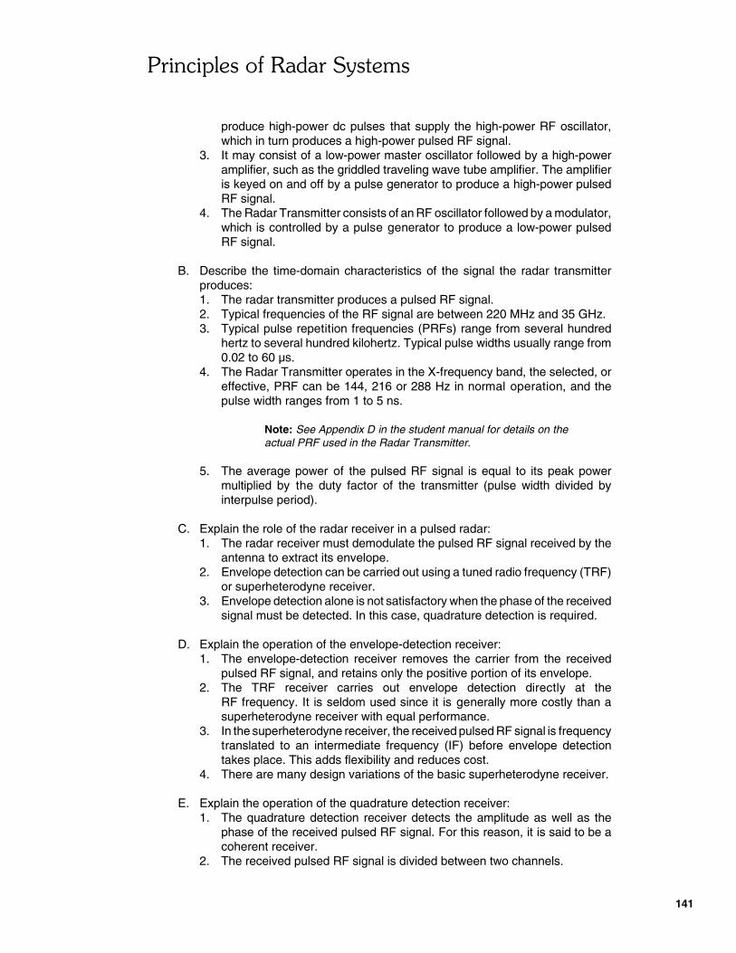
�������������������� �����
141
produce high-power dc pulses that supply the high-power RF oscillator,which in turn produces a high-power pulsed RF signal.
3. It may consist of a low-power master oscillator followed by a high-poweramplifier, such as the griddled traveling wave tube amplifier. The amplifieris keyed on and off by a pulse generator to produce a high-power pulsedRF signal.
4. The Radar Transmitter consists of an RF oscillator followed by a modulator,which is controlled by a pulse generator to produce a low-power pulsedRF signal.
B. Describe the time-domain characteristics of the signal the radar transmitterproduces:1. The radar transmitter produces a pulsed RF signal.2. Typical frequencies of the RF signal are between 220 MHz and 35 GHz.3. Typical pulse repetition frequencies (PRFs) range from several hundred
hertz to several hundred kilohertz. Typical pulse widths usually range from0.02 to 60 µs.
4. The Radar Transmitter operates in the X-frequency band, the selected, oreffective, PRF can be 144, 216 or 288 Hz in normal operation, and thepulse width ranges from 1 to 5 ns.
Note: See Appendix D in the student manual for details on theactual PRF used in the Radar Transmitter.
5. The average power of the pulsed RF signal is equal to its peak powermultiplied by the duty factor of the transmitter (pulse width divided byinterpulse period).
C. Explain the role of the radar receiver in a pulsed radar:1. The radar receiver must demodulate the pulsed RF signal received by the
antenna to extract its envelope.2. Envelope detection can be carried out using a tuned radio frequency (TRF)
or superheterodyne receiver.3. Envelope detection alone is not satisfactory when the phase of the received
signal must be detected. In this case, quadrature detection is required.
D. Explain the operation of the envelope-detection receiver:1. The envelope-detection receiver removes the carrier from the received
pulsed RF signal, and retains only the positive portion of its envelope.2. The TRF receiver carries out envelope detection directly at the
RF frequency. It is seldom used since it is generally more costly than asuperheterodyne receiver with equal performance.
3. In the superheterodyne receiver, the received pulsed RF signal is frequencytranslated to an intermediate frequency (IF) before envelope detectiontakes place. This adds flexibility and reduces cost.
4. There are many design variations of the basic superheterodyne receiver.
E. Explain the operation of the quadrature detection receiver:1. The quadrature detection receiver detects the amplitude as well as the
phase of the received pulsed RF signal. For this reason, it is said to be acoherent receiver.
2. The received pulsed RF signal is divided between two channels.
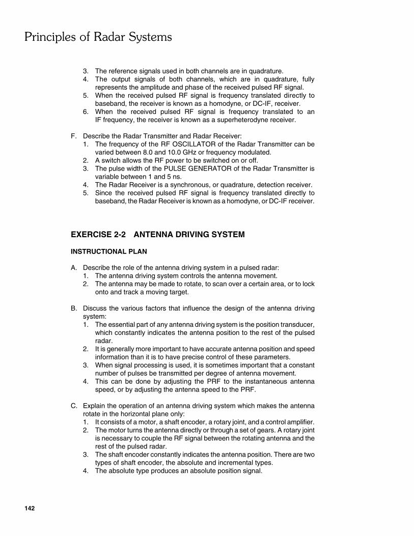
�������������������� �����
142
3. The reference signals used in both channels are in quadrature.4. The output signals of both channels, which are in quadrature, fully
represents the amplitude and phase of the received pulsed RF signal.5. When the received pulsed RF signal is frequency translated directly to
baseband, the receiver is known as a homodyne, or DC-IF, receiver.6. When the received pulsed RF signal is frequency translated to an
IF frequency, the receiver is known as a superheterodyne receiver.
F. Describe the Radar Transmitter and Radar Receiver:1. The frequency of the RF OSCILLATOR of the Radar Transmitter can be
varied between 8.0 and 10.0 GHz or frequency modulated.2. A switch allows the RF power to be switched on or off.3. The pulse width of the PULSE GENERATOR of the Radar Transmitter is
variable between 1 and 5 ns.4. The Radar Receiver is a synchronous, or quadrature, detection receiver.5. Since the received pulsed RF signal is frequency translated directly to
baseband, the Radar Receiver is known as a homodyne, or DC-IF receiver.
EXERCISE 2-2 ANTENNA DRIVING SYSTEM
INSTRUCTIONAL PLAN
A. Describe the role of the antenna driving system in a pulsed radar:1. The antenna driving system controls the antenna movement.2. The antenna may be made to rotate, to scan over a certain area, or to lock
onto and track a moving target.
B. Discuss the various factors that influence the design of the antenna drivingsystem:1. The essential part of any antenna driving system is the position transducer,
which constantly indicates the antenna position to the rest of the pulsedradar.
2. It is generally more important to have accurate antenna position and speedinformation than it is to have precise control of these parameters.
3. When signal processing is used, it is sometimes important that a constantnumber of pulses be transmitted per degree of antenna movement.
4. This can be done by adjusting the PRF to the instantaneous antennaspeed, or by adjusting the antenna speed to the PRF.
C. Explain the operation of an antenna driving system which makes the antennarotate in the horizontal plane only:1. It consists of a motor, a shaft encoder, a rotary joint, and a control amplifier.2. The motor turns the antenna directly or through a set of gears. A rotary joint
is necessary to couple the RF signal between the rotating antenna and therest of the pulsed radar.
3. The shaft encoder constantly indicates the antenna position. There are twotypes of shaft encoder, the absolute and incremental types.
4. The absolute type produces an absolute position signal.
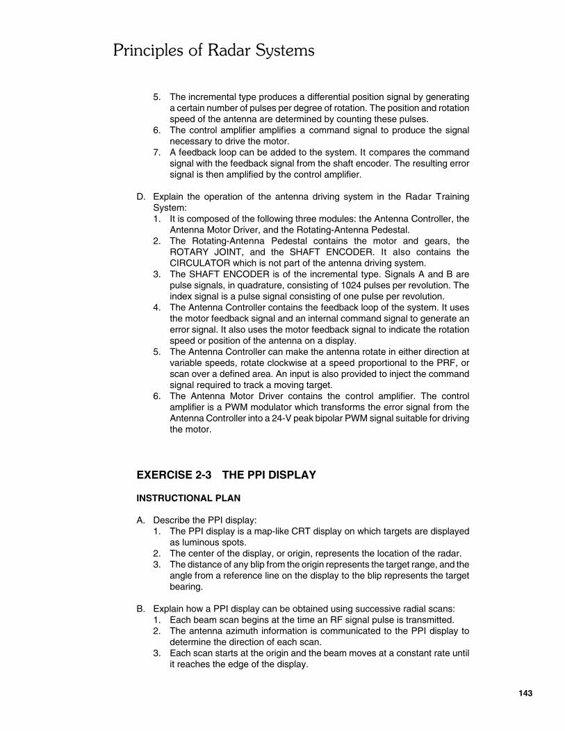
�������������������� �����
143
5. The incremental type produces a differential position signal by generatinga certain number of pulses per degree of rotation. The position and rotationspeed of the antenna are determined by counting these pulses.
6. The control amplifier amplifies a command signal to produce the signalnecessary to drive the motor.
7. A feedback loop can be added to the system. It compares the commandsignal with the feedback signal from the shaft encoder. The resulting errorsignal is then amplified by the control amplifier.
D. Explain the operation of the antenna driving system in the Radar TrainingSystem:1. It is composed of the following three modules: the Antenna Controller, the
Antenna Motor Driver, and the Rotating-Antenna Pedestal.2. The Rotating-Antenna Pedestal contains the motor and gears, the
ROTARY JOINT, and the SHAFT ENCODER. It also contains theCIRCULATOR which is not part of the antenna driving system.
3. The SHAFT ENCODER is of the incremental type. Signals A and B arepulse signals, in quadrature, consisting of 1024 pulses per revolution. Theindex signal is a pulse signal consisting of one pulse per revolution.
4. The Antenna Controller contains the feedback loop of the system. It usesthe motor feedback signal and an internal command signal to generate anerror signal. It also uses the motor feedback signal to indicate the rotationspeed or position of the antenna on a display.
5. The Antenna Controller can make the antenna rotate in either direction atvariable speeds, rotate clockwise at a speed proportional to the PRF, orscan over a defined area. An input is also provided to inject the commandsignal required to track a moving target.
6. The Antenna Motor Driver contains the control amplifier. The controlamplifier is a PWM modulator which transforms the error signal from theAntenna Controller into a 24-V peak bipolar PWM signal suitable for drivingthe motor.
EXERCISE 2-3 THE PPI DISPLAY
INSTRUCTIONAL PLAN
A. Describe the PPI display:1. The PPI display is a map-like CRT display on which targets are displayed
as luminous spots.2. The center of the display, or origin, represents the location of the radar.3. The distance of any blip from the origin represents the target range, and the
angle from a reference line on the display to the blip represents the targetbearing.
B. Explain how a PPI display can be obtained using successive radial scans:1. Each beam scan begins at the time an RF signal pulse is transmitted.2. The antenna azimuth information is communicated to the PPI display to
determine the direction of each scan.3. Each scan starts at the origin and the beam moves at a constant rate until
it reaches the edge of the display.
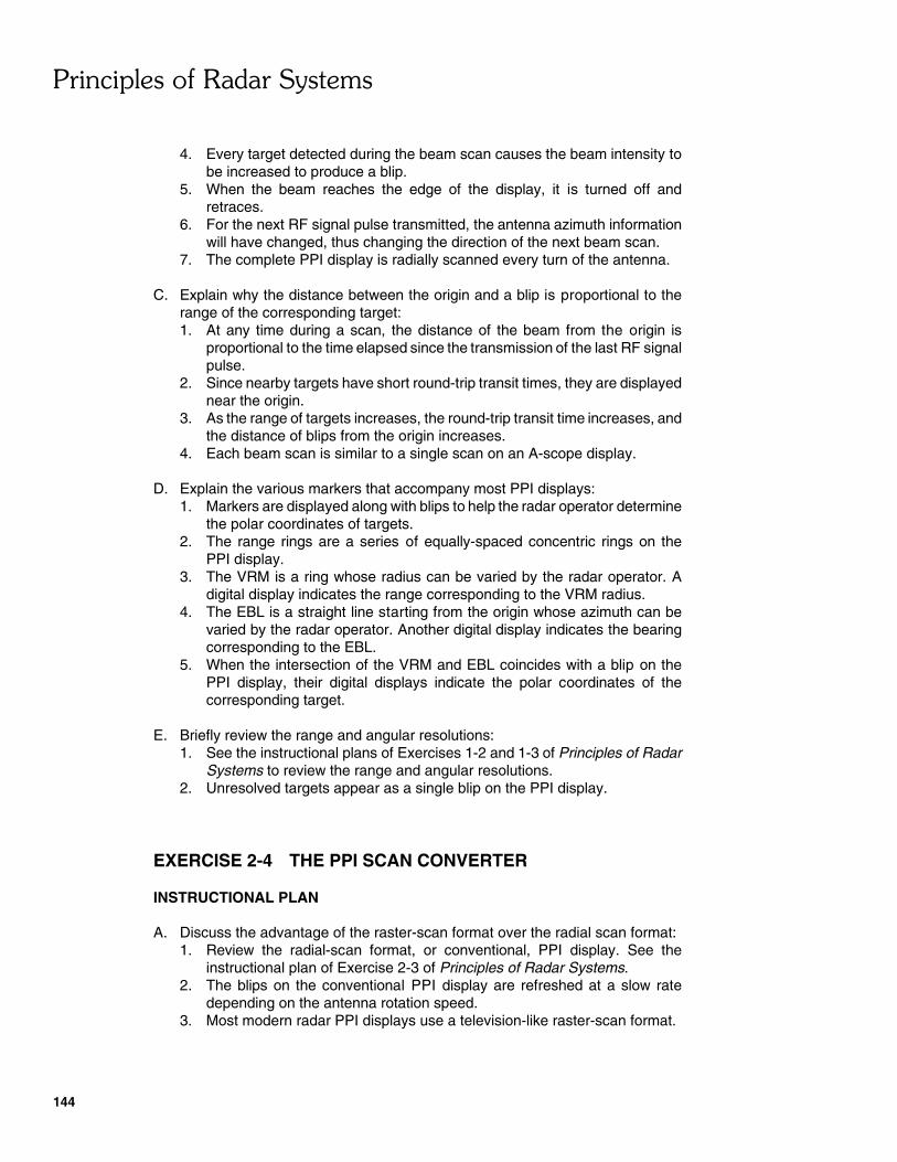
�������������������� �����
144
4. Every target detected during the beam scan causes the beam intensity tobe increased to produce a blip.
5. When the beam reaches the edge of the display, it is turned off andretraces.
6. For the next RF signal pulse transmitted, the antenna azimuth informationwill have changed, thus changing the direction of the next beam scan.
7. The complete PPI display is radially scanned every turn of the antenna.
C. Explain why the distance between the origin and a blip is proportional to therange of the corresponding target:1. At any time during a scan, the distance of the beam from the origin is
proportional to the time elapsed since the transmission of the last RF signalpulse.
2. Since nearby targets have short round-trip transit times, they are displayednear the origin.
3. As the range of targets increases, the round-trip transit time increases, andthe distance of blips from the origin increases.
4. Each beam scan is similar to a single scan on an A-scope display.
D. Explain the various markers that accompany most PPI displays:1. Markers are displayed along with blips to help the radar operator determine
the polar coordinates of targets.2. The range rings are a series of equally-spaced concentric rings on the
PPI display.3. The VRM is a ring whose radius can be varied by the radar operator. A
digital display indicates the range corresponding to the VRM radius.4. The EBL is a straight line starting from the origin whose azimuth can be
varied by the radar operator. Another digital display indicates the bearingcorresponding to the EBL.
5. When the intersection of the VRM and EBL coincides with a blip on thePPI display, their digital displays indicate the polar coordinates of thecorresponding target.
E. Briefly review the range and angular resolutions:1. See the instructional plans of Exercises 1-2 and 1-3 of Principles of Radar
Systems to review the range and angular resolutions.2. Unresolved targets appear as a single blip on the PPI display.
EXERCISE 2-4 THE PPI SCAN CONVERTER
INSTRUCTIONAL PLAN
A. Discuss the advantage of the raster-scan format over the radial scan format:1. Review the radial-scan format, or conventional, PPI display. See the
instructional plan of Exercise 2-3 of Principles of Radar Systems.2. The blips on the conventional PPI display are refreshed at a slow rate
depending on the antenna rotation speed.3. Most modern radar PPI displays use a television-like raster-scan format.
�������������������� �����
145
4. The faster refresh rate of this type of scan format with respect to that of theradial-scan format produces a stable display which is less fatiguing to lookat.
5. The raster-scan format facilitates the generation of markers.
B. Explain the role and operating principle of a digital scan converter:1. A scan-format conversion is necessary to produce a PPI display with a
raster-scan format.2. In most modern radars, this task is carried out using a digital scan
converter.3. The acquisition/write section of the digital scan converter writes the video
data in a memory by addressing its cells radially.4. The read/display section of the digital scan converter reads the video data
from the memory by scanning its cells in a raster-scan format to producethe PPI display.
C. Explain the operation of the acquisition/write section of the PPI Scan Converter:1. This section of the PPI Scan Converter consists of the functional blocks
connected to the VIDEO INPUT, TRIGGER INPUTS, and AZIMUTHINPUT.
2. During each write scan, the write circuitry addresses the MEMORY cellsradially using rectangular coordinates.
3. Each write scan is triggered by the PRF signal. This signal is delayed bythe VIDEO DELAY COMPENSATOR to compensate for the delayintroduced in the video signal by the signal processing circuitry.
4. The delayed PRF signal resets the RADIAL POSITION GENERATORwhich generates the range information.
5. The rectangular coordinates are calculated from the range and azimuthinformation by the POLAR TO RECTANGULAR CONVERTER.
6. The THRESHOLD COMPARATOR detects the pulses in the VIDEO INPUTsignal that exceed its threshold level to transform them into TTL-levelpulses.
D. Explain the operation of the read/display section of the PPI Scan Converter:1. This section of the PPI Scan Converter consists of the two ADDRESS
GENERATORs, the CLOCK GENERATOR, the TIMING CIRCUIT, and thecircuitry driving the OUTPUTS TO SCOPE.
2. The read circuitry addresses the MEMORY cells in a raster-scan format.3. Each ADDRESS GENERATOR produces a series of addresses, from the
lowest to the highest. Both series of addresses address the MEMORYcells.
4. Each cell containing a logical 1 causes a pixel to be illuminated on theCRT display.
5. The X and Y SWEEP GENERATORs carry out the horizontal and verticalscanning of the CRT display, respectively, according to the addressing ofthe MEMORY cells.
6. The MARKER GENERATOR produces the markers. These are added tothe video data from the MEMORY by the LOGIC ADDER.
7. The LEVEL CONVERTER adjusts the level of the video data from theLOGIC ADDER so that this signal is suitable to drive the Z-axis of anoscilloscope.
�������������������� �����
146
DEMONSTRATIONS
• Measurement of the radar wavelength with the A-scope display– Set up and calibrate the pulsed radar with the A-scope display. Set the
RF OSCILLATOR frequency to 10.0 GHz.– Using the POSITION MODE of the Target Controller and a flat plate target,
observe that the amplitude of the target blip varies as the target rangevaries.
– Using the Target Controller, measure the target range variation betweentwo positive maxima or two negative maxima of the target blip amplitude.Double this result to obtain the radar wavelength. The result should beclose to 3 cm, which is the radar wavelength � for a 10-GHz frequency.
– Decrease the RF OSCILLATOR frequency to 8.0 GHz, then repeat themeasurement. Compare the results using � = c/ft.
• Frequency-domain observation of the various signals of the Radar Transmitter– A spectrum analyzer having a frequency range of at least 12 GHz, and a
frequency span of at least 200 MHz/div. is required to carry out thefollowing observations.
– Connect the CW/FM-CW RF OUTPUT to the spectrum analyzer, andobserve the characteristics of the RF OSCILLATOR signal frequencyspectrum. Vary the RF OSCILLATOR frequency, and observe the effect onthe frequency spectrum.
– Connect the PULSE GENERATOR OUTPUT to the spectrum analyzer, andobserve the characteristics of the pulse signal frequency spectrum. Varythe PRF and the pulse width of the PULSE GENERATOR, and observe theeffects on the frequency spectrum.
– Connect the PULSED RF OUTPUT to the spectrum analyzer, and observethe characteristics of the pulsed RF signal frequency spectrum. Vary theRF OSCILLATOR frequency, the PRF, and the pulse width of the PULSEGENERATOR, and observe the effects on the frequency spectrum.
Note: When the entire frequency spectrum of the pulsedRF signal is observed on the spectrum analyzer, it may be partlyor completely lost in noise. This is more likely to happen with the1- and 2-ns pulse widths. This problem may be resolved byinserting a wideband amplifier between the PULSEDRF OUTPUT and the spectrum analyzer input. The widebandamplifier should have a gain of 20 to 30 dB, over a frequencyrange of 7 to 11 GHz.
• Observation of target blips and of the parasitic blips affecting the pulsed radarsimultaneously on the A-scope display and PPI display.– Set up and calibrate the pulsed radar with the PPI display. Use any of the
available observation ranges.
– Connect another oscilloscope to the Dual-Channel Sampler to obtain the A-scope display.
Note: Since the observation range origin of the pulsed radar has beencalibrated with the PPI display, the blips may appear at slightly incorrectranges on the A-scope display.
�������������������� �����
147
– Decrease the GAIN of the Analog MTI Processor to minimum to clean upthe PPI display.
– Using the MANual ANTENNA ROTATION MODE of the AntennaController, set the rotation speed of the Radar Antenna to approximately1 r/min, and then set the GAIN of the Analog MTI Processor so that blipsappear on the PPI display.
– Observe that when the Radar Antenna points to targets, blips appear brieflyon the A-scope display, whereas they are recorded on the PPI display andcan be visualized anytime.
– Set the rotation speed of the Radar Antenna to approximately 5 r/min, andthen slightly decalibrate the origin of the observation range in order toobserve the parasitic blips on both displays.
– Observe that the parasitic blips appear as a group of pulses on the A-scopedisplay. Since these pulses are present regardless the Radar Antennaposition, thick concentric circles appear on the PPI display.
PRESENTATION AIDS
1. Review the New Terms after the unit DISCUSSION OF FUNDAMENTALS.2. Explain that the pulsed RF signal is similar to an ASK signal, except that an RF-
frequency carrier and very short-duration modulating pulses are used. Theirfrequency spectra have the same shape.
3. Describe the operation of mixers in both the time and frequency domains.4. Show that the I- and Q-channel outputs of a quadrature detector fully represent
the amplitude A and the phase � of the received signal:
If I = A cos �Q = A sin �
then A = I 2� Q 2
� = arctan (Q/I)
5. Use timing diagrams to explain the operation of the acquisition/write andread/display sections of the PPI Scan Converter.
6. Discuss the various uses of pulsed radars with a PPI display.


.�����$���!
Barton, D. K., and Leonov, S.A., eds., radar Technology Encyclopedia, Norwood,MA: Artech House, 1997.ISBN: 0-89006-893-3
Carpentier, Michel H., Radars, Bases Modernes, 4e édition, Masson, Paris, 1981ISBN: 2-225-74624-9
Eaves, J.L. and Reedy, E.K., Principles of Modern Radar, Van Nostrand ReinholdCompany Inc., New York, 1987ISBN: 0-442-22104-5
Nathanson, Fred E., Radar Design Principles, McGraw-Hill Book Company,New York, 1969.
Schleher, D.C., Introduction to Electronic Warfare, Norwood, MA: Artech House,1986.ISBN: 0-89006-142-4
Schleher, D.C., Electronic Warfare in the Information Age, Norwood, MA: ArtechHouse, 1999.ISBN: 0-89006-526-8
Skolnik, M. I., Introduction to Radar Systems, 2nd edition, McGraw-Hill Book Co.,New Yord, 1980.ISBN: 0-07-057909-1
Stimson, G. W., Introduction to Airborne Radar, 2nd ed., Mendham, NJ: SciTechPublishing, 1998.ISBN; 1-891121-01-4