Embed Size (px)
Citation preview
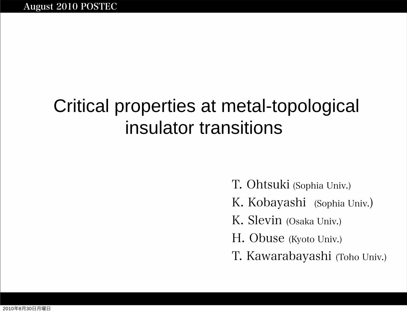
August 2010 POSTEC
Critical properties at metal-topological insulator transitions
T. Ohtsuki (Sophia Univ.)K. Kobayashi (Sophia Univ.)K. Slevin (Osaka Univ.)H. Obuse (Kyoto Univ.)T. Kawarabayashi (Toho Univ.)
2010年8月30日月曜日
Critical conductance distributions at the localization-delocalization transitionsAugust 2010 POSTEC Critical properties at metal-topological insulator transitions
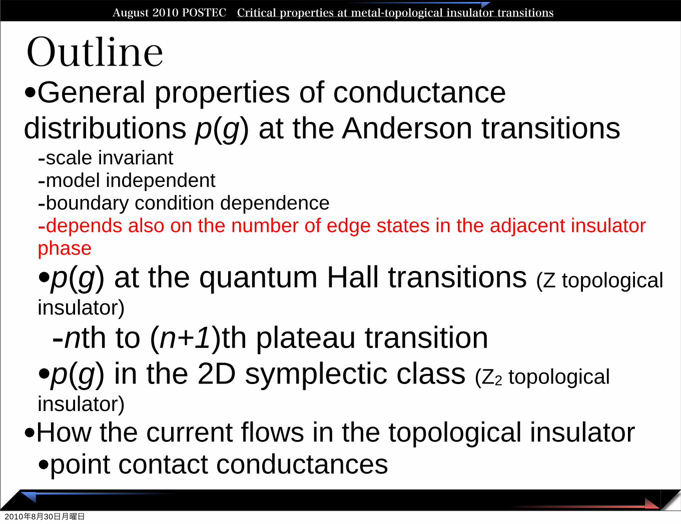
Outline•General properties of conductance distributions p(g) at the Anderson transitions
-scale invariant-model independent-boundary condition dependence-depends also on the number of edge states in the adjacent insulator phase
•p(g) at the quantum Hall transitions (Z topological insulator)
-nth to (n+1)th plateau transition •p(g) in the 2D symplectic class (Z2 topological insulator)
•How the current flows in the topological insulator•point contact conductances
2010年8月30日月曜日

Critical conductance distributions at the localization-delocalization transitionsAugust 2010 POSTEC Critical properties at metal-topological insulator transitions
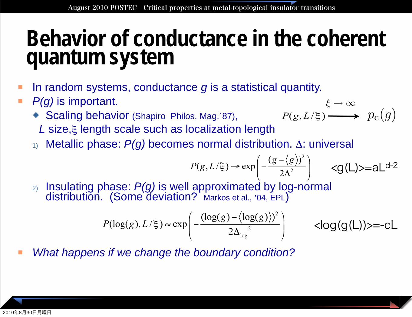
Behavior of conductance in the coherent quantum system
In random systems, conductance g is a statistical quantity. P(g) is important.
Scaling behavior (Shapiro Philos. Mag.’87), L size,ξ length scale such as localization length
1) Metallic phase: P(g) becomes normal distribution. Δ: universal
2) Insulating phase: P(g) is well approximated by log-normal distribution. (Some deviation? Markos et al., ’04, EPL)
What happens if we change the boundary condition?
<g(L)>=aLd-2
<log(g(L))>=-cL
2010年8月30日月曜日
Critical conductance distributions at the localization-delocalization transitionsAugust 2010 POSTEC Critical properties at metal-topological insulator transitions
Behavior of conductance in the coherent quantum system
In random systems, conductance g is a statistical quantity. P(g) is important.
Scaling behavior (Shapiro Philos. Mag.’87), L size,ξ length scale such as localization length
1) Metallic phase: P(g) becomes normal distribution. Δ: universal
2) Insulating phase: P(g) is well approximated by log-normal distribution. (Some deviation? Markos et al., ’04, EPL)
What happens if we change the boundary condition?
pc(g)
pc(g)
! ! "
<g(L)>=aLd-2
<log(g(L))>=-cL
2010年8月30日月曜日
Critical conductance distributions at the localization-delocalization transitionsAugust 2010 POSTEC Critical properties at metal-topological insulator transitions
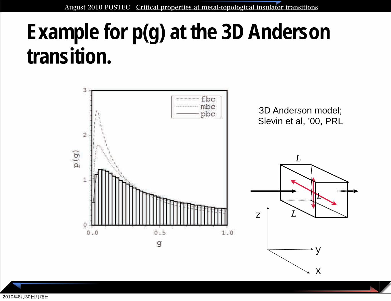
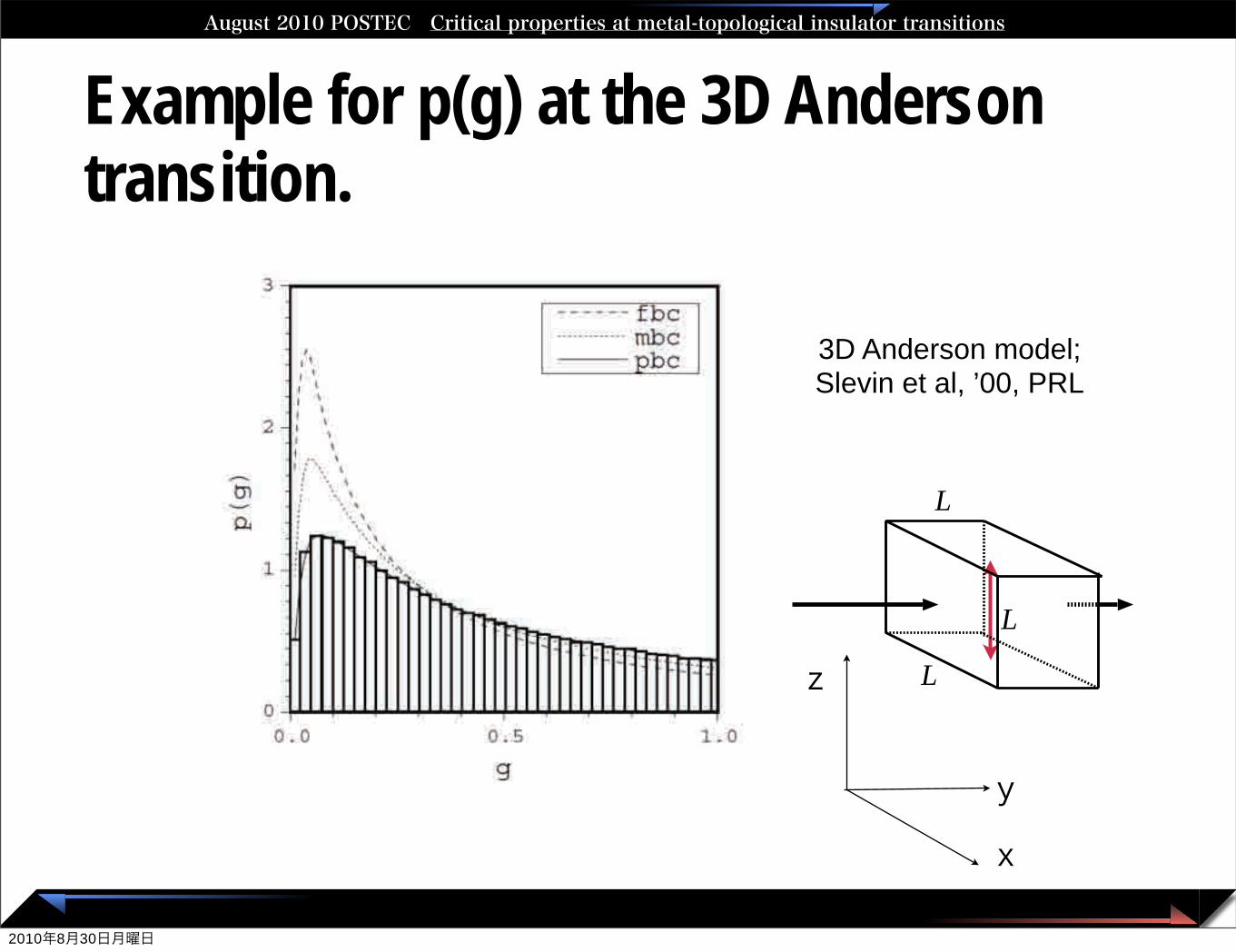
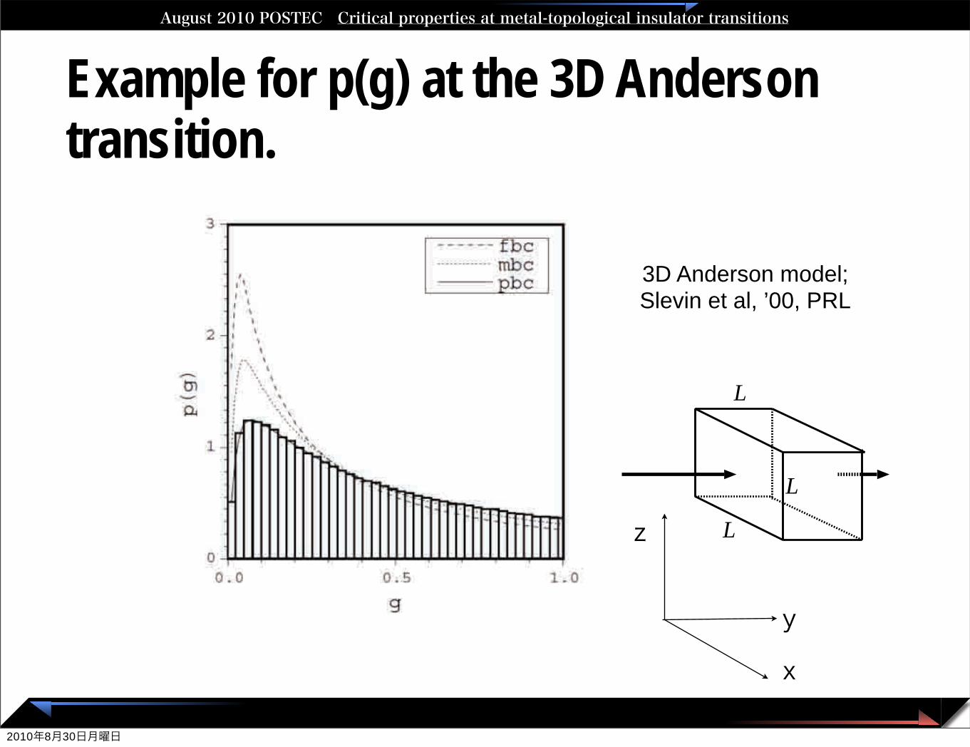
Example for p(g) at the 3D Anderson transition.
3D Anderson model;Slevin et al, ’00, PRL
L
L
L
x
y
z
2010年8月30日月曜日
Critical conductance distributions at the localization-delocalization transitionsAugust 2010 POSTEC Critical properties at metal-topological insulator transitions
Example for p(g) at the 3D Anderson transition.
3D Anderson model;Slevin et al, ’00, PRL
L
L
L
x
y
z
2010年8月30日月曜日
Critical conductance distributions at the localization-delocalization transitionsAugust 2010 POSTEC Critical properties at metal-topological insulator transitions
Example for p(g) at the 3D Anderson transition.
3D Anderson model;Slevin et al, ’00, PRL
L
L
L
x
y
z
2010年8月30日月曜日
Critical conductance distributions at the localization-delocalization transitionsAugust 2010 POSTEC Critical properties at metal-topological insulator transitions
July 2008 Bremen
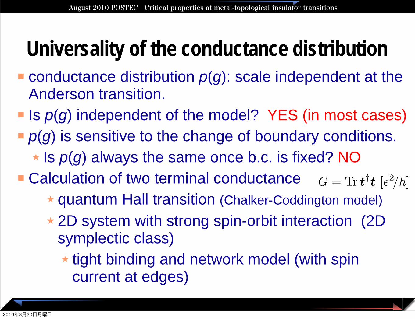
Universality of the conductance distribution conductance distribution p(g): scale independent at the
Anderson transition. Is p(g) independent of the model? YES (in most cases) p(g) is sensitive to the change of boundary conditions.
★ Is p(g) always the same once b.c. is fixed? NO Calculation of two terminal conductance
★ quantum Hall transition (Chalker-Coddington model)★ 2D system with strong spin-orbit interaction (2D
symplectic class)★ tight binding and network model (with spin
current at edges)
s =!
ei!2 00 ei!4
"!r tt !r
"!ei!1 00 ei!3
". (8)
#!R
$=
Nx%
i=1
T (i)#!L
$, !R = T (M) · · ·T (2)T (1) !L !out = S !in (9)
G =h
e2g = Tr t†t G = Tr t†t [e2/h]
G ! G! = Tr t†t ! Tr t!†t! (10)= Tr (t†t!r†r) ! Tr (t!†t!r!†r!) (11)= Tr I(N+1)"(N+1) ! Tr IN"N (12)= 1 (13)
G > 1 (14)
t(N+1)"(N+1) = U
&
''''''(
"1 0 · · · 0
0 "2
......
. . ."N 0
0 · · · 0 1
)
******+V (15)
0.1 Perfectly conducting channel in unitary class
In the unitary case, a PCC arises from the asymmetry of the number of the incomingand outgoing channels [?]. On the left side, the network has N + 1 incoming and N
outgoing channels. Hence the reflection matrix r has the dimension (N + 1) " N .Because
rank (r†r)(N+1)"(N+1) = rank rN"(N+1) # N, (16)
there is at least one reflection eigenvalue ‘0’. That implies the existence of a PCC.
0.2 Perfectly conducting channel in symplectic class
In the symplectic case, a PCC arises from the odd number of the dimension of thereflection matrices. The symplectic symmetry requires that
S = !ST. (17)
Then it follows thatr = !rT, (18)
and by taking its determinant,
det(r) = det(!rT) = (!1)2N+1 det(r) = 0. (19)
Thereforerank r(2N+1)"(2N+1) # 2N. (20)
Thus r has at least one eigenvalue ‘0’ and there exists a PCC.
2010年8月30日月曜日
Critical conductance distributions at the localization-delocalization transitionsAugust 2010 POSTEC Critical properties at metal-topological insulator transitions
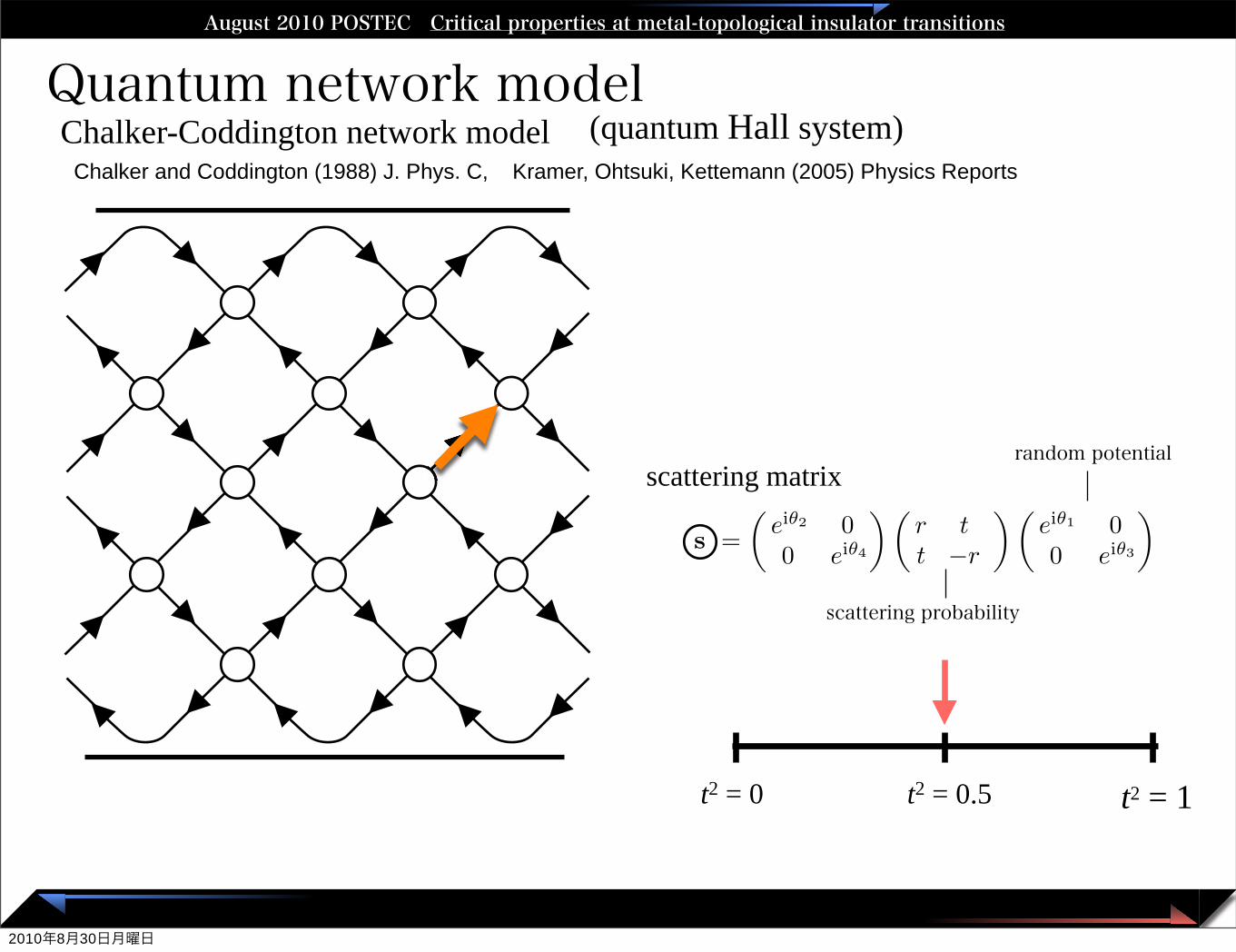
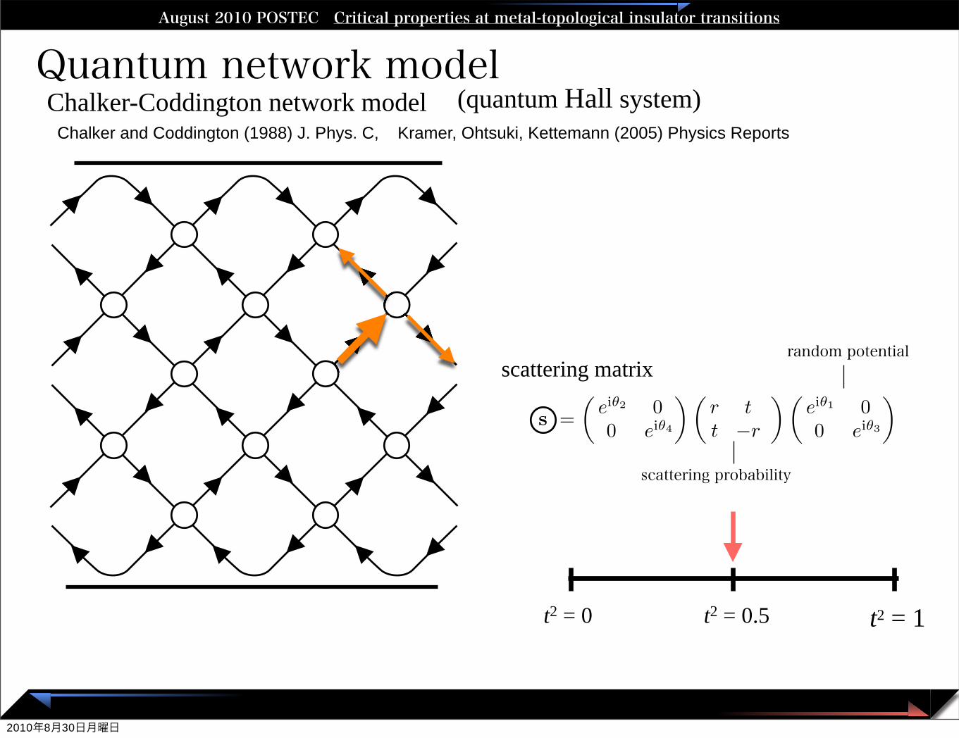
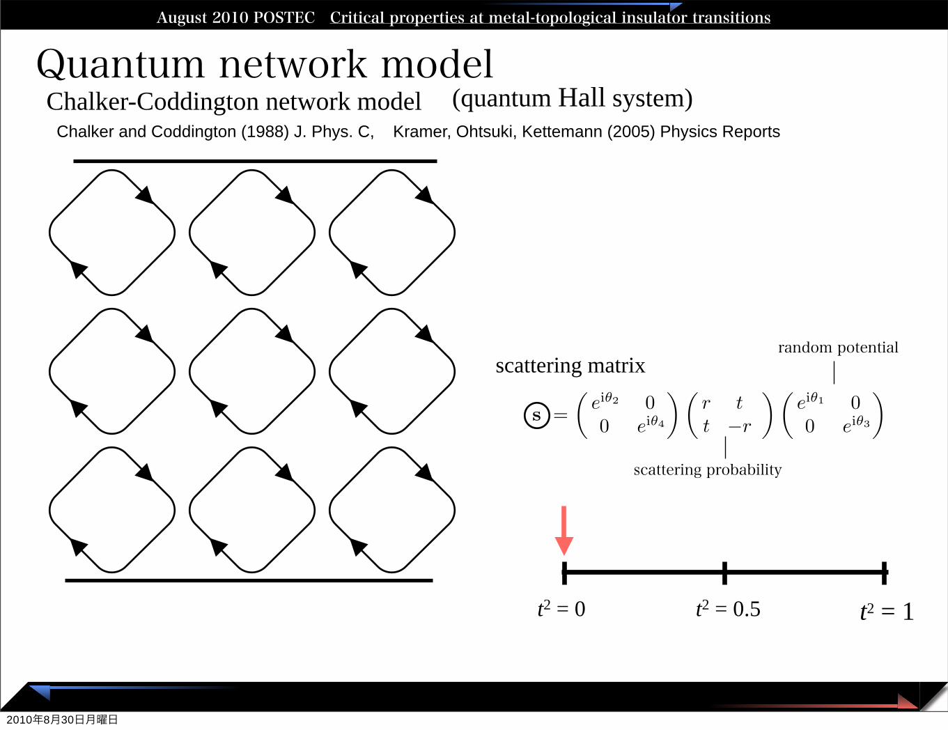
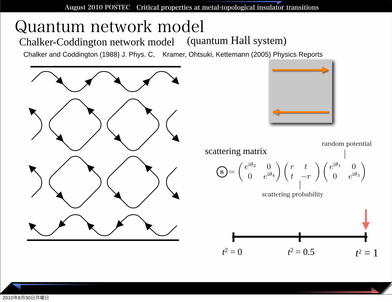
Quantum network modelChalker and Coddington (1988) J. Phys. C, Kramer, Ohtsuki, Kettemann (2005) Physics Reports
s =!
ei!2 00 ei!4
"!r tt !r
"!ei!1 00 ei!3
". (8)
scattering matrixrandom potential
scattering probability
Chalker-Coddington network model
t2 = 1t2 = 0 t2 = 0.5
(quantum Hall system)
2010年8月30日月曜日
Critical conductance distributions at the localization-delocalization transitionsAugust 2010 POSTEC Critical properties at metal-topological insulator transitions
Quantum network modelChalker and Coddington (1988) J. Phys. C, Kramer, Ohtsuki, Kettemann (2005) Physics Reports
s =!
ei!2 00 ei!4
"!r tt !r
"!ei!1 00 ei!3
". (8)
scattering matrixrandom potential
scattering probability
Chalker-Coddington network model
t2 = 1t2 = 0 t2 = 0.5
(quantum Hall system)Chalker and Coddington (1988) J. Phys. C, Kramer, Ohtsuki, Kettemann (2005) Physics Reports
2010年8月30日月曜日
Critical conductance distributions at the localization-delocalization transitionsAugust 2010 POSTEC Critical properties at metal-topological insulator transitions
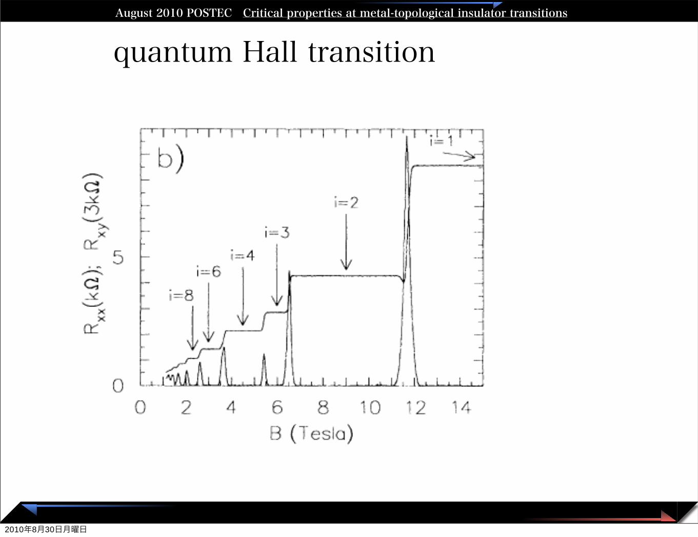
quantum Hall transition
2010年8月30日月曜日
Critical conductance distributions at the localization-delocalization transitionsAugust 2010 POSTEC Critical properties at metal-topological insulator transitions
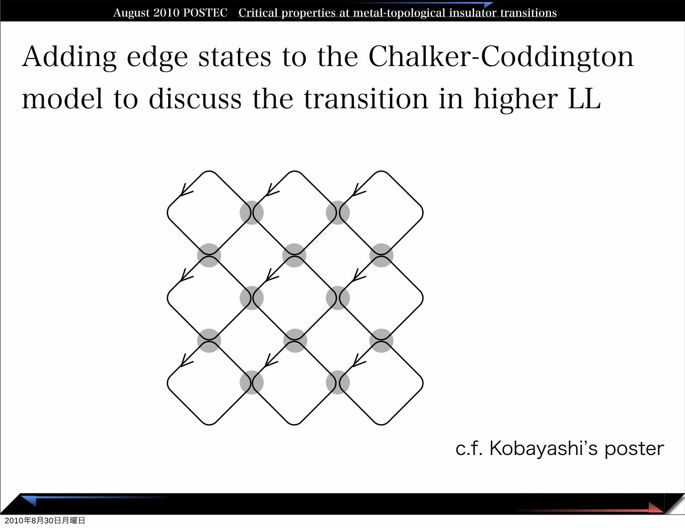
Adding edge states to the Chalker-Coddington model to discuss the transition in higher LL
c.f. Kobayashi’s poster
2010年8月30日月曜日
Critical conductance distributions at the localization-delocalization transitionsAugust 2010 POSTEC Critical properties at metal-topological insulator transitions
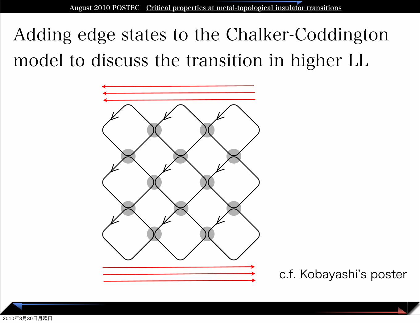
Adding edge states to the Chalker-Coddington model to discuss the transition in higher LL
c.f. Kobayashi’s poster
2010年8月30日月曜日
Critical conductance distributions at the localization-delocalization transitionsAugust 2010 POSTEC Critical properties at metal-topological insulator transitions
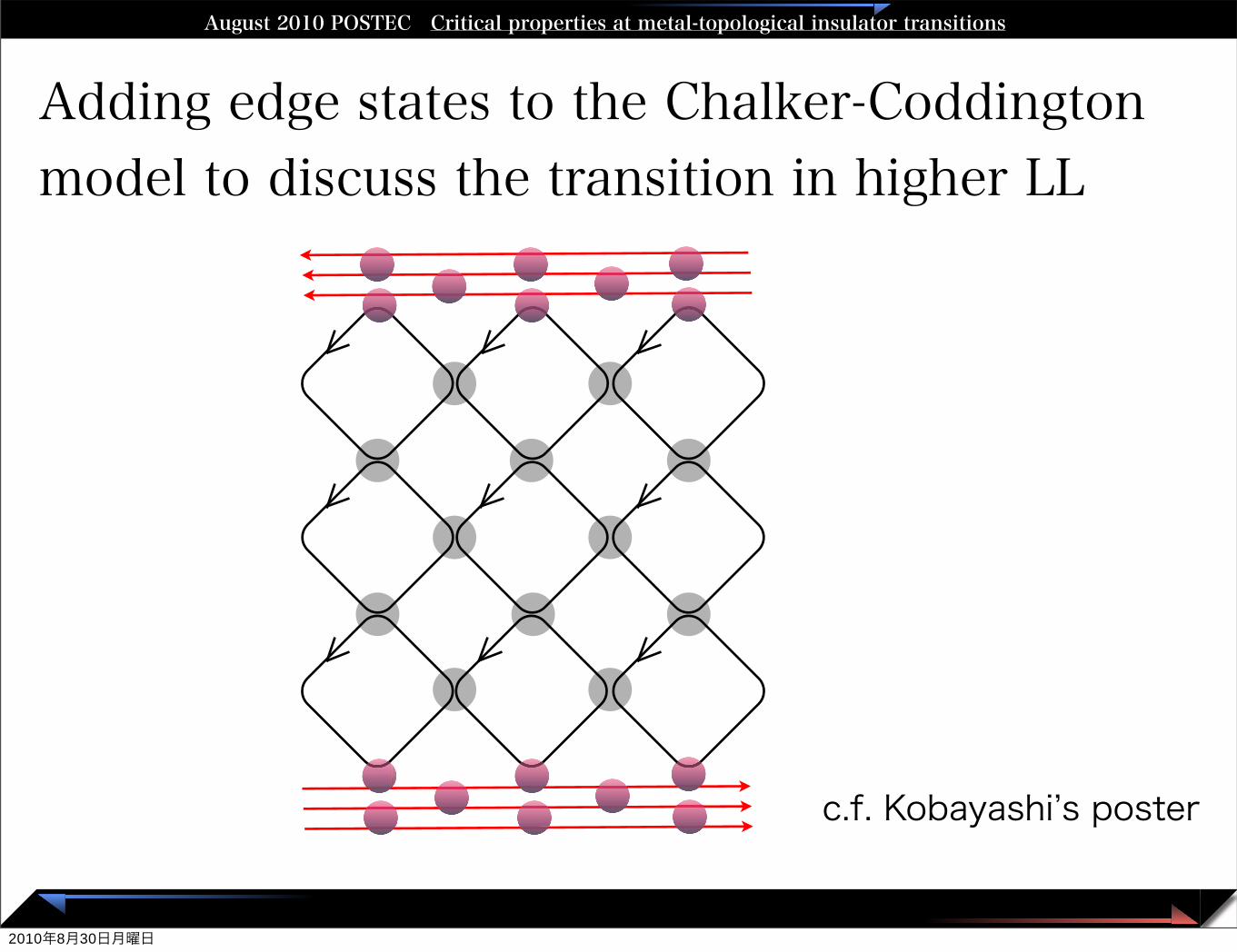
Adding edge states to the Chalker-Coddington model to discuss the transition in higher LL
c.f. Kobayashi’s poster
2010年8月30日月曜日
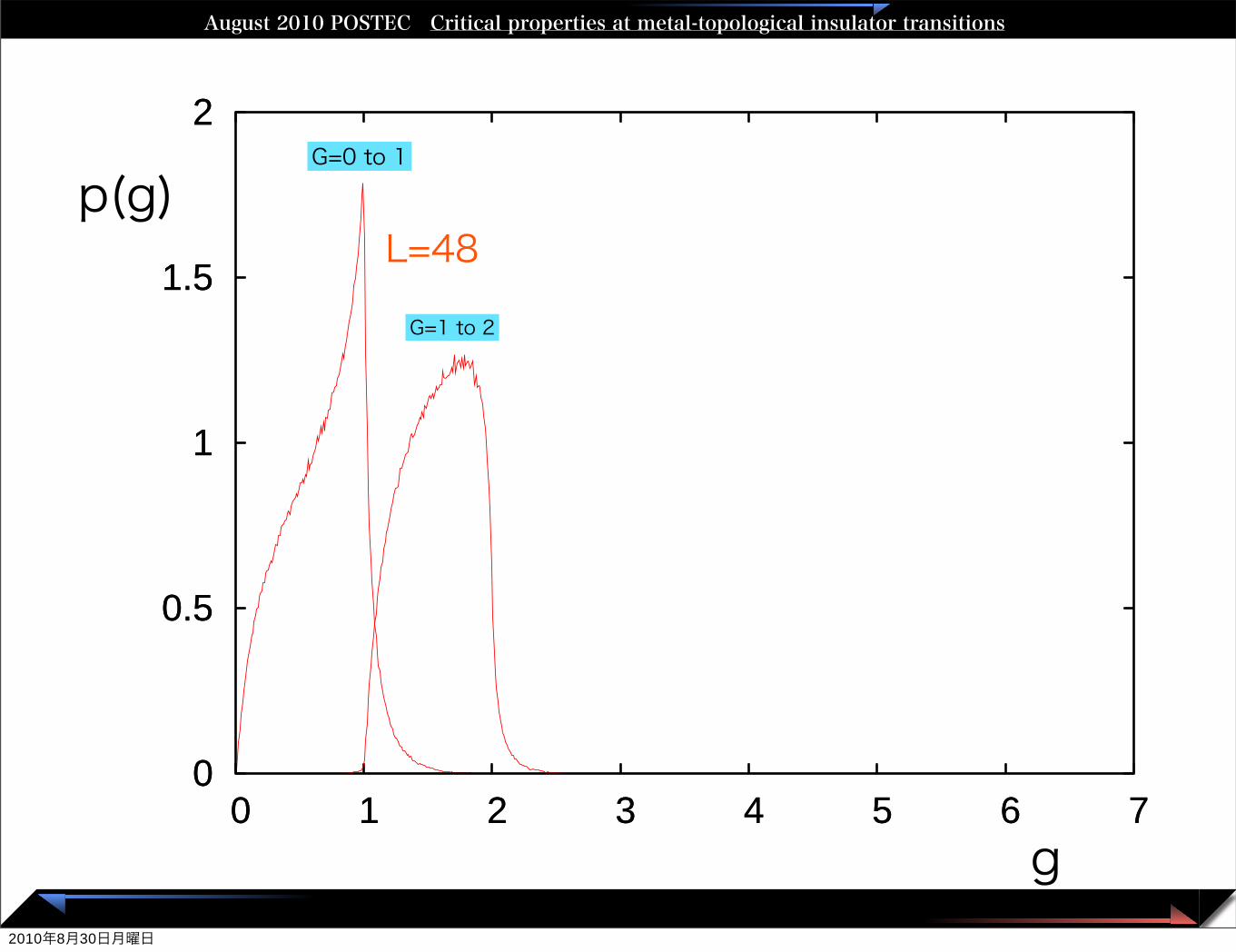
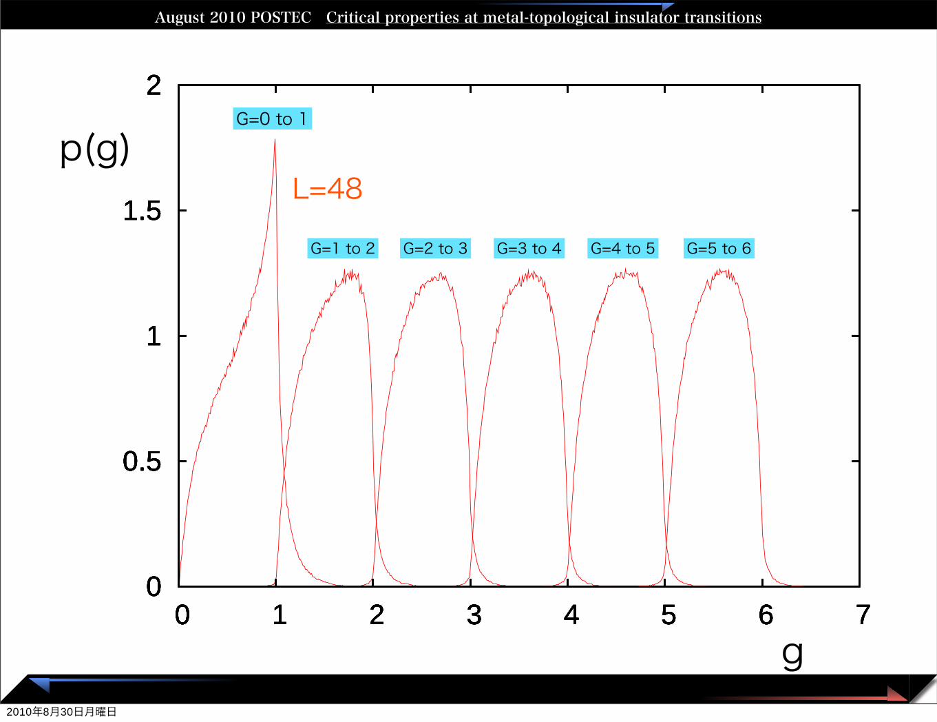
Critical conductance distributions at the localization-delocalization transitionsAugust 2010 POSTEC Critical properties at metal-topological insulator transitions
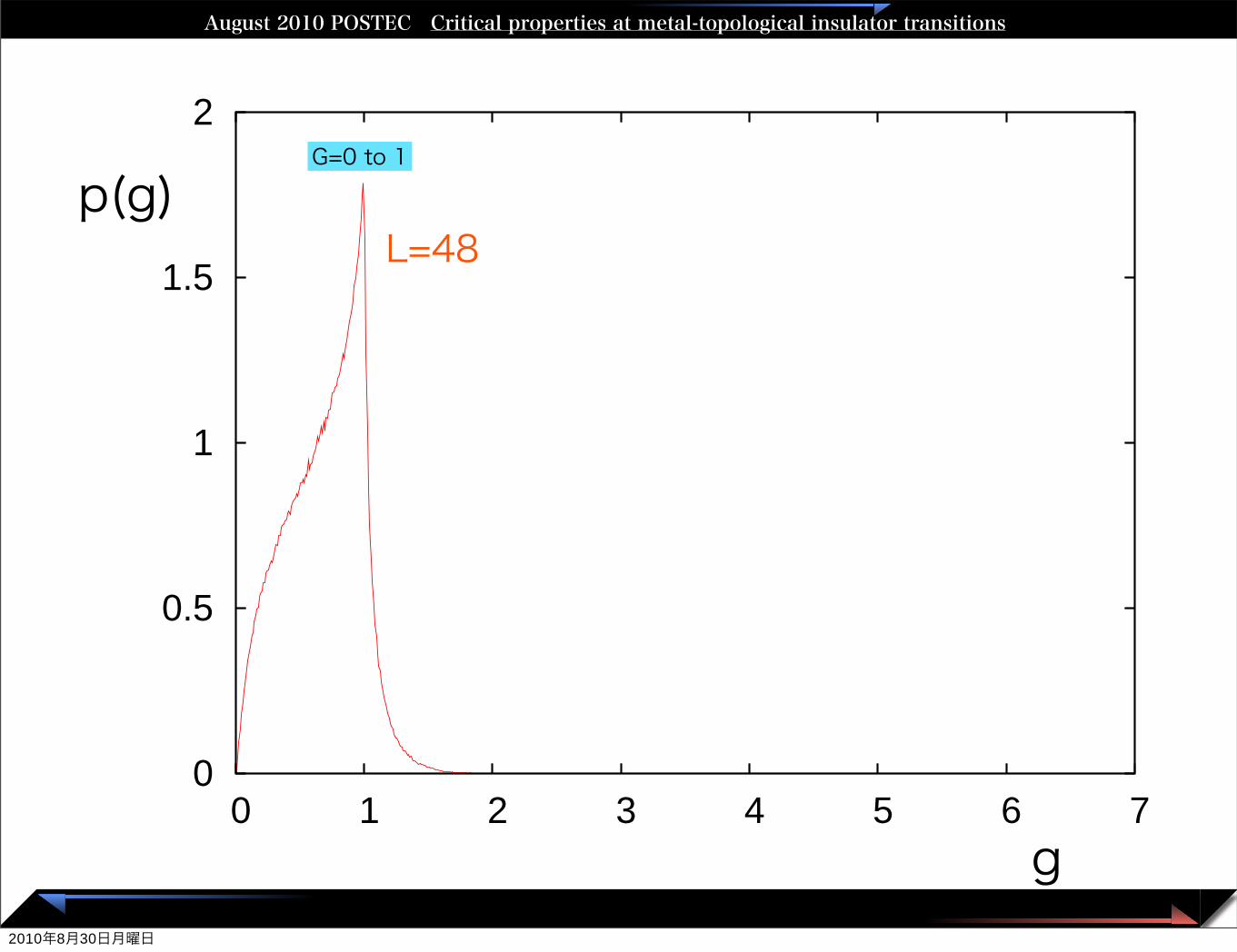
L=48
0
0.5
1
1.5
2
0 1 2 3 4 5 6 7
G=0 to 1
g
p(g)
2010年8月30日月曜日
Critical conductance distributions at the localization-delocalization transitionsAugust 2010 POSTEC Critical properties at metal-topological insulator transitions
L=48
0
0.5
1
1.5
2
0 1 2 3 4 5 6 7
G=0 to 1
0
0.5
1
1.5
2
0 1 2 3 4 5 6 7
G=1 to 2
g
p(g)
2010年8月30日月曜日
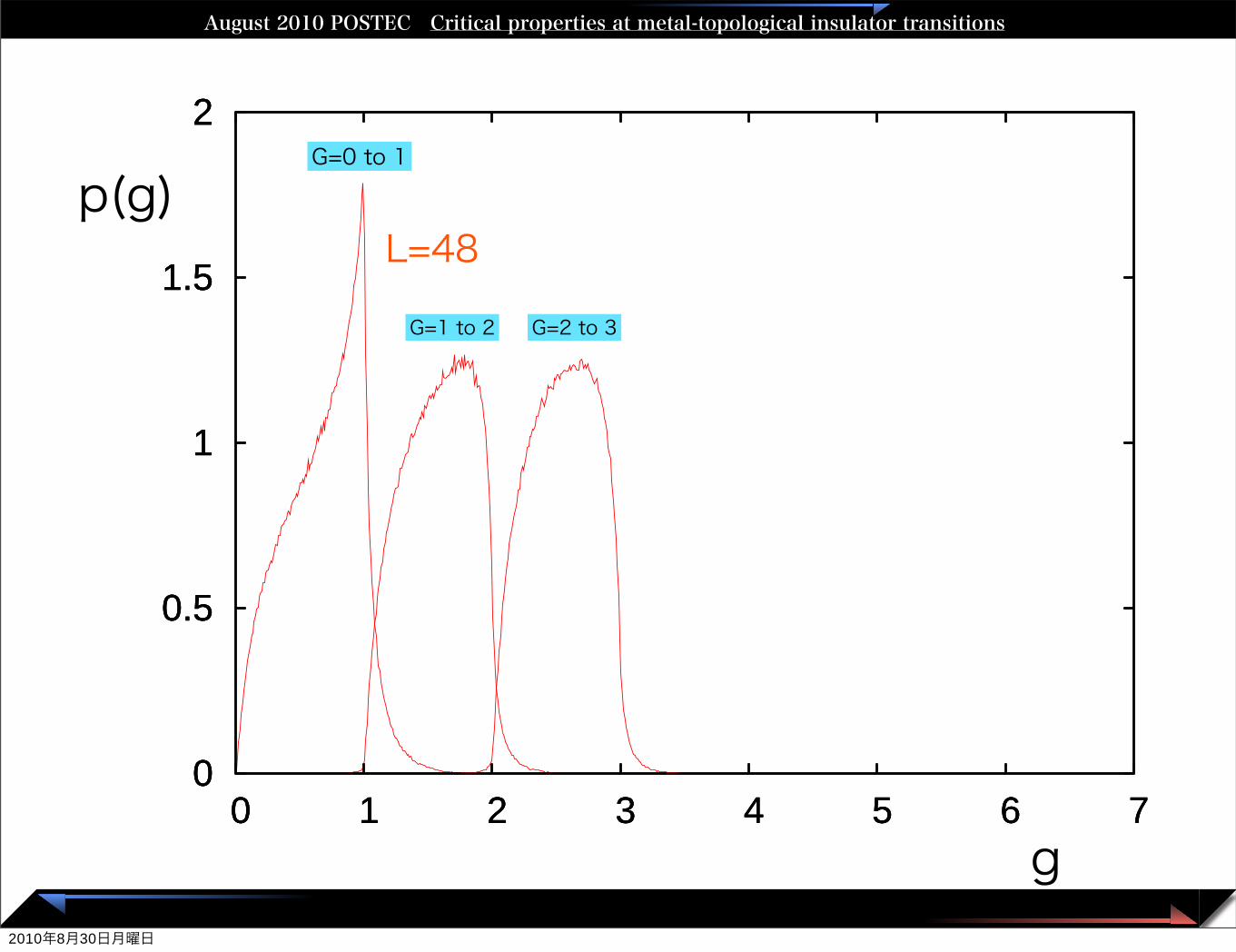
Critical conductance distributions at the localization-delocalization transitionsAugust 2010 POSTEC Critical properties at metal-topological insulator transitions
L=48
0
0.5
1
1.5
2
0 1 2 3 4 5 6 7
G=0 to 1
0
0.5
1
1.5
2
0 1 2 3 4 5 6 7
G=1 to 2
0
0.5
1
1.5
2
0 1 2 3 4 5 6 7
G=2 to 3
g
p(g)
2010年8月30日月曜日
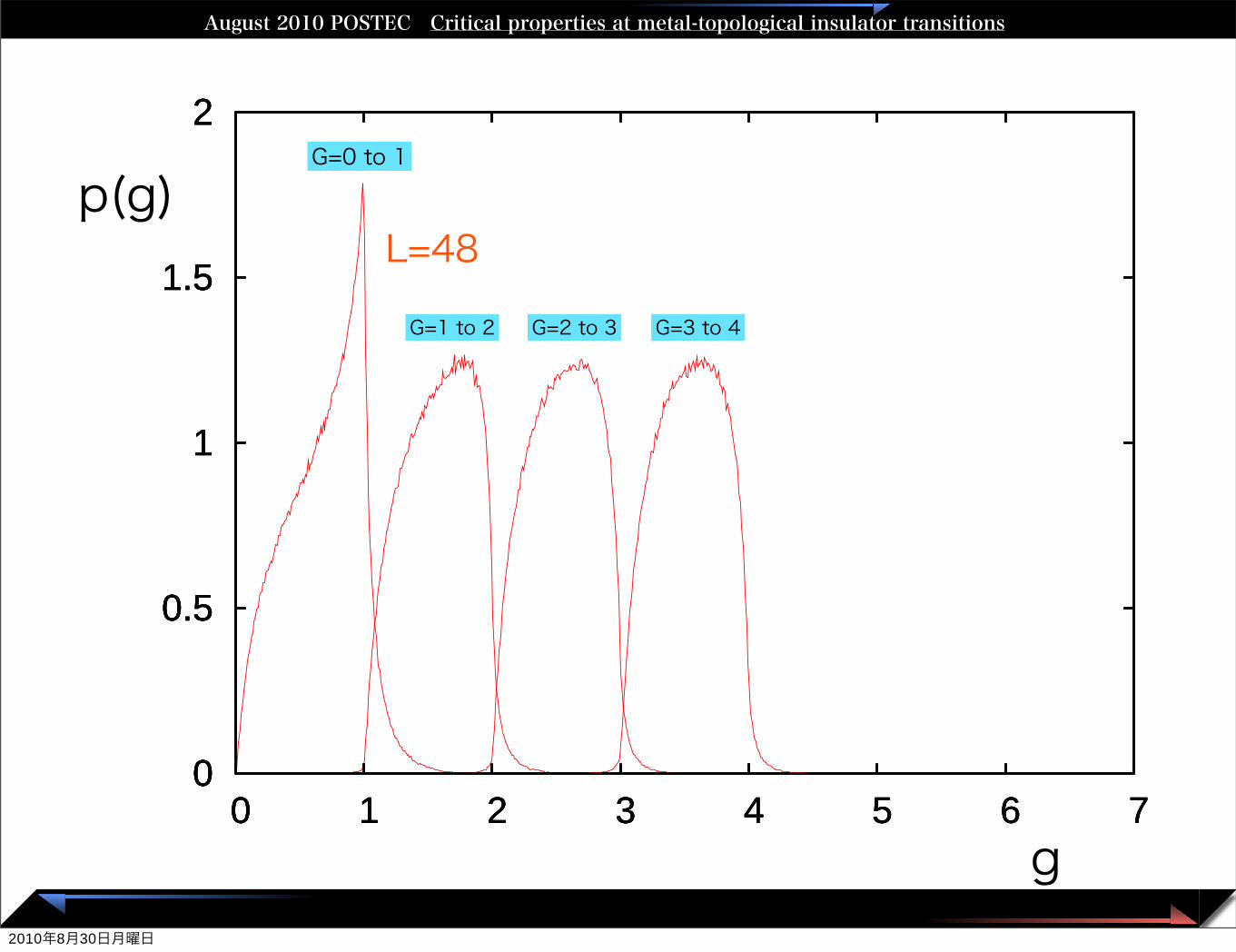
Critical conductance distributions at the localization-delocalization transitionsAugust 2010 POSTEC Critical properties at metal-topological insulator transitions
L=48
0
0.5
1
1.5
2
0 1 2 3 4 5 6 7
G=0 to 1
0
0.5
1
1.5
2
0 1 2 3 4 5 6 7
G=1 to 2
0
0.5
1
1.5
2
0 1 2 3 4 5 6 7
G=2 to 3
0
0.5
1
1.5
2
0 1 2 3 4 5 6 7
G=3 to 4
g
p(g)
2010年8月30日月曜日
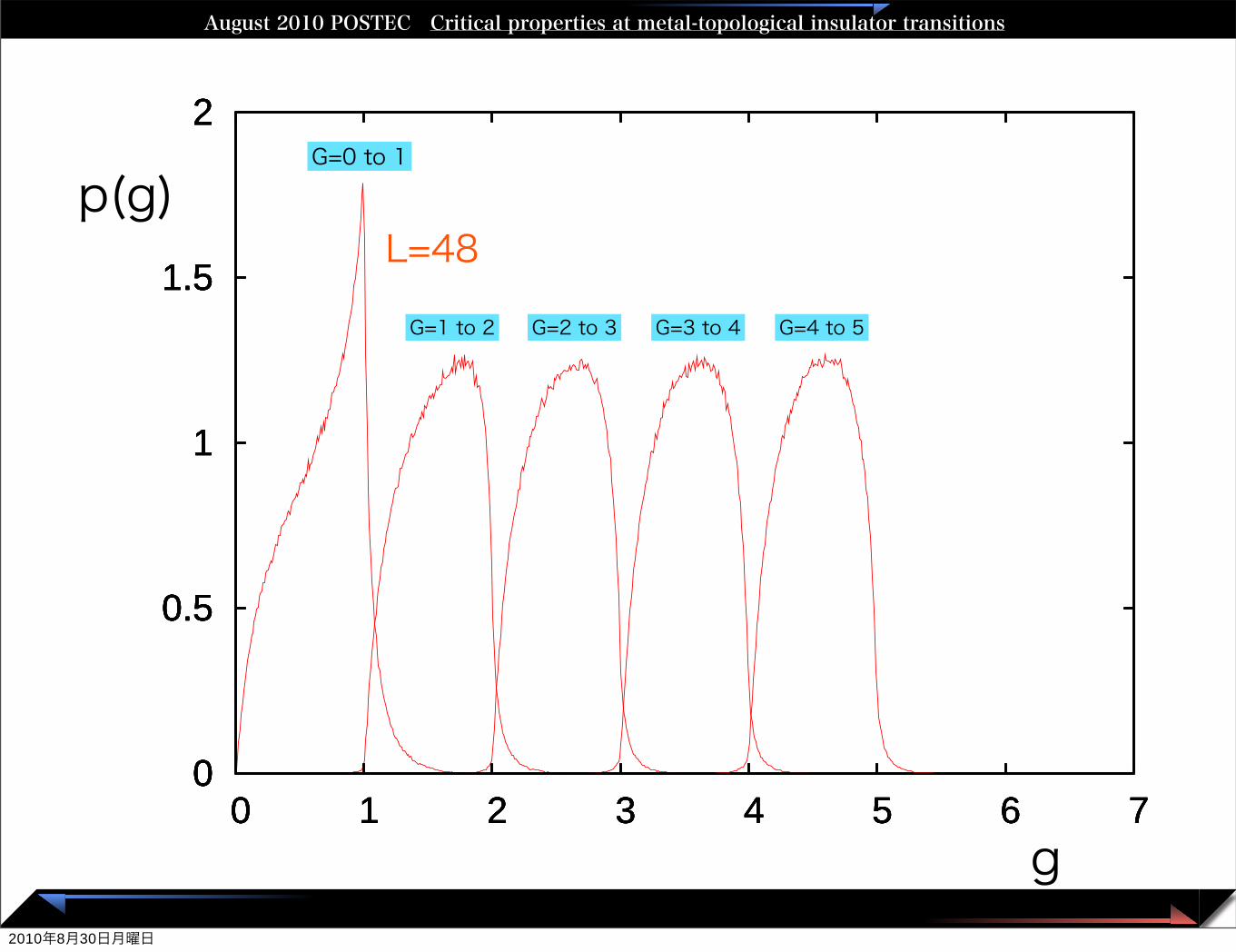
Critical conductance distributions at the localization-delocalization transitionsAugust 2010 POSTEC Critical properties at metal-topological insulator transitions
L=48
0
0.5
1
1.5
2
0 1 2 3 4 5 6 7
G=0 to 1
0
0.5
1
1.5
2
0 1 2 3 4 5 6 7
G=1 to 2
0
0.5
1
1.5
2
0 1 2 3 4 5 6 7
G=2 to 3
0
0.5
1
1.5
2
0 1 2 3 4 5 6 7
G=3 to 4
0
0.5
1
1.5
2
0 1 2 3 4 5 6 7
G=4 to 5
g
p(g)
2010年8月30日月曜日
Critical conductance distributions at the localization-delocalization transitionsAugust 2010 POSTEC Critical properties at metal-topological insulator transitions
L=48
0
0.5
1
1.5
2
0 1 2 3 4 5 6 7
G=0 to 1
0
0.5
1
1.5
2
0 1 2 3 4 5 6 7
G=1 to 2
0
0.5
1
1.5
2
0 1 2 3 4 5 6 7
G=2 to 3
0
0.5
1
1.5
2
0 1 2 3 4 5 6 7
G=3 to 4
0
0.5
1
1.5
2
0 1 2 3 4 5 6 7
G=4 to 5
0
0.5
1
1.5
2
0 1 2 3 4 5 6 7
G=5 to 6
g
p(g)
2010年8月30日月曜日
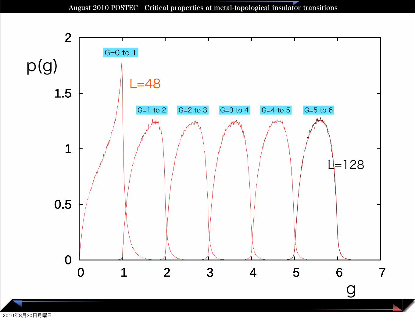
Critical conductance distributions at the localization-delocalization transitionsAugust 2010 POSTEC Critical properties at metal-topological insulator transitions
L=48
0
0.5
1
1.5
2
0 1 2 3 4 5 6 7
L=128
0
0.5
1
1.5
2
0 1 2 3 4 5 6 7
G=0 to 1
0
0.5
1
1.5
2
0 1 2 3 4 5 6 7
G=1 to 2
0
0.5
1
1.5
2
0 1 2 3 4 5 6 7
G=2 to 3
0
0.5
1
1.5
2
0 1 2 3 4 5 6 7
G=3 to 4
0
0.5
1
1.5
2
0 1 2 3 4 5 6 7
G=4 to 5
0
0.5
1
1.5
2
0 1 2 3 4 5 6 7
G=5 to 6
g
p(g)
2010年8月30日月曜日
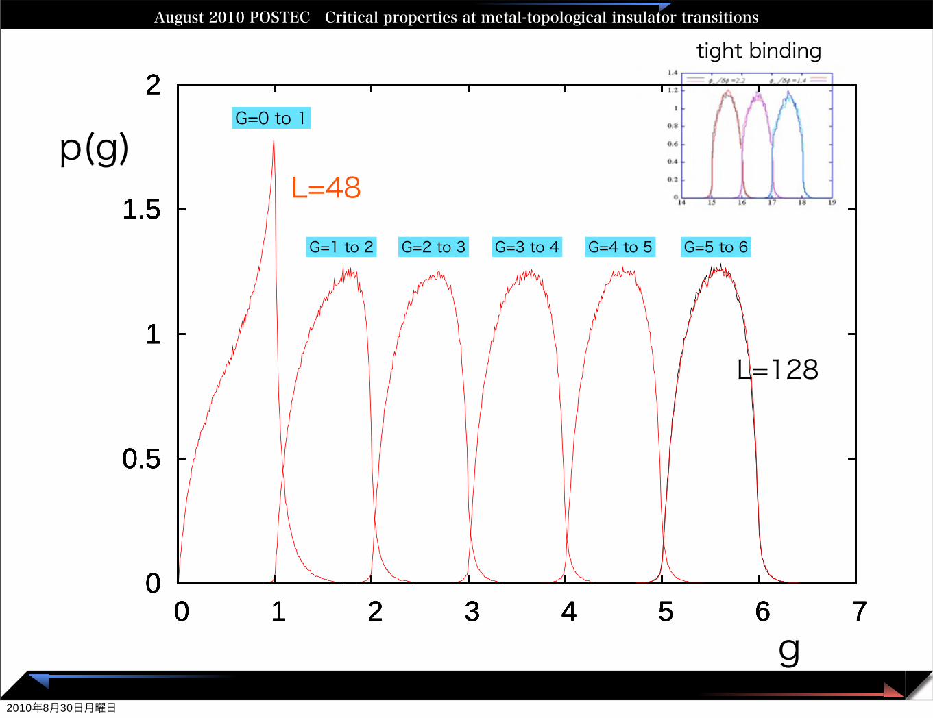
Critical conductance distributions at the localization-delocalization transitionsAugust 2010 POSTEC Critical properties at metal-topological insulator transitions
L=48
0
0.5
1
1.5
2
0 1 2 3 4 5 6 7
L=128
tight binding
0
0.5
1
1.5
2
0 1 2 3 4 5 6 7
G=0 to 1
0
0.5
1
1.5
2
0 1 2 3 4 5 6 7
G=1 to 2
0
0.5
1
1.5
2
0 1 2 3 4 5 6 7
G=2 to 3
0
0.5
1
1.5
2
0 1 2 3 4 5 6 7
G=3 to 4
0
0.5
1
1.5
2
0 1 2 3 4 5 6 7
G=4 to 5
0
0.5
1
1.5
2
0 1 2 3 4 5 6 7
G=5 to 6
g
p(g)
2010年8月30日月曜日
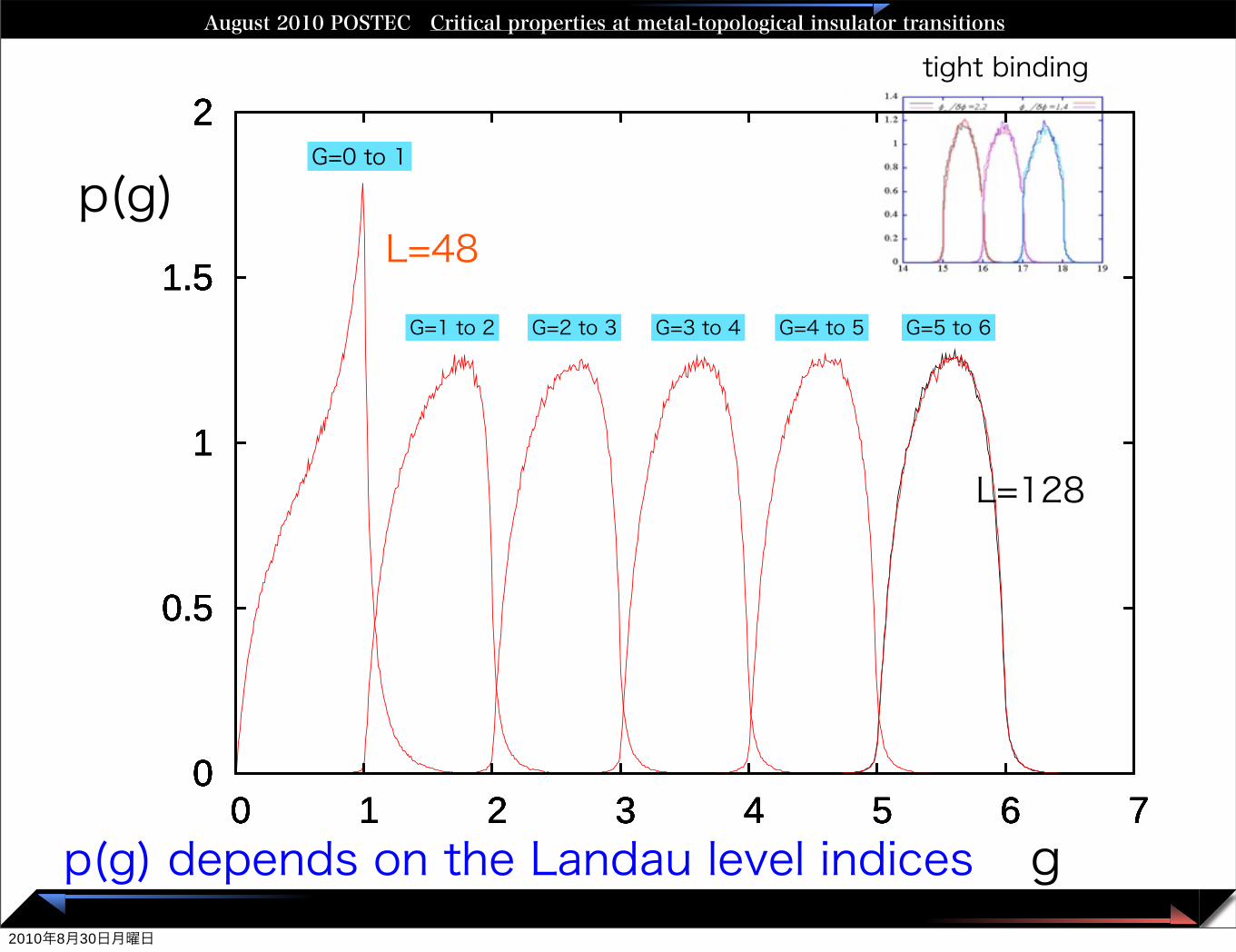
Critical conductance distributions at the localization-delocalization transitionsAugust 2010 POSTEC Critical properties at metal-topological insulator transitions
L=48
0
0.5
1
1.5
2
0 1 2 3 4 5 6 7
L=128
tight binding
0
0.5
1
1.5
2
0 1 2 3 4 5 6 7
G=0 to 1
0
0.5
1
1.5
2
0 1 2 3 4 5 6 7
G=1 to 2
0
0.5
1
1.5
2
0 1 2 3 4 5 6 7
G=2 to 3
0
0.5
1
1.5
2
0 1 2 3 4 5 6 7
G=3 to 4
0
0.5
1
1.5
2
0 1 2 3 4 5 6 7
G=4 to 5
0
0.5
1
1.5
2
0 1 2 3 4 5 6 7
G=5 to 6
g
p(g)
p(g) depends on the Landau level indices2010年8月30日月曜日
Critical conductance distributions at the localization-delocalization transitionsAugust 2010 POSTEC Critical properties at metal-topological insulator transitions
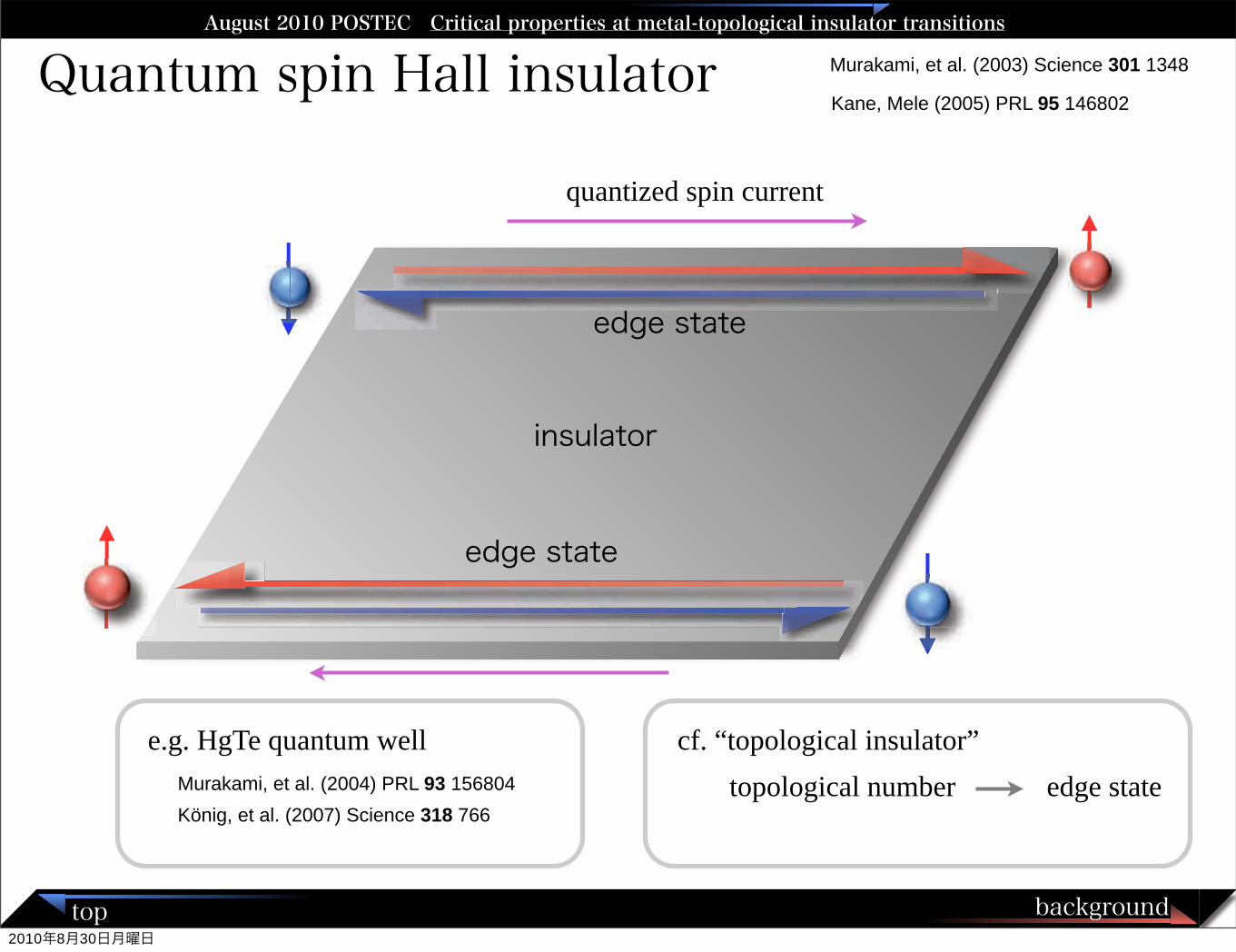
Quantum spin Hall insulator
e.g. HgTe quantum welltopological number
background
Murakami, et al. (2003) Science 301 1348
top
König, et al. (2007) Science 318 766 Murakami, et al. (2004) PRL 93 156804
Kane, Mele (2005) PRL 95 146802
quantized spin current
cf. “topological insulator”edge state
insulator
edge state
edge state
2010年8月30日月曜日
Critical conductance distributions at the localization-delocalization transitionsAugust 2010 POSTEC Critical properties at metal-topological insulator transitions
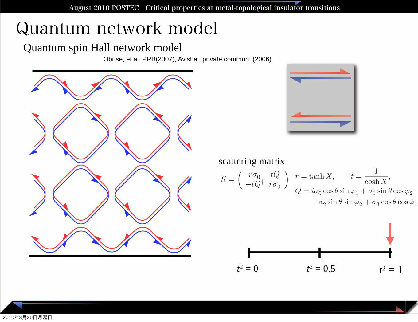
Quantum network modelQuantum spin Hall network model
Obuse, et al. PRB(2007), Avishai, private commun. (2006)
2
FIG. 1: (Color online) Elementary building blocks of the net-work model. A square Bravais lattice with nearest-neighborsites connected by bonds underlies the construction of thenetwork model. Any red site of one of the two sublattices ofthe square lattice is replaced by a red circle S (a node of typeS) with the four bonds meeting at the site replaced by fourpairs of directed links numbered according to the rule shownin (a). Any blue site of the complementary sublattice of thesquare lattice is replaced by a blue circle S
! (a node of typeS!) with the four bonds meeting at the site replaced by four
pairs of directed links numbered according to the rule shownin (b). Observe that a clockwise rotation by !/2 turn (a) into(b). The directed links represent incoming or outgoing planewaves with a well-defined projection of the spin-1/2 quantumnumber along the quantization axis. Each pair of links re-placing a bond represents a Kramers doublet of plane waves.Each node S or S
! depicts a scattering process represented bya 4!4 unitary matrix defined in Eq. (2.1) that preserves time-reversal symmetry (TRS) but breaks spin-rotation symmetry(SRS).
tum number ! =!. A link represented by a dashed linecarries the spin-1/2 quantum number ! =". Third, thefour pairs of directed links that meet at a node are la-beled according to the rules of Fig. 1(a) and Fig. 1(b)if the node is of type S and S
!, respectively. With theconventions of Figs. 1(a) and 1(b) either node defines a4# 4 scattering matrix S that preserves TRS but breaksthe SRS and can be represented by
!
"
"
"
"
#
"(o)1"
"(o)2#
"(o)3"
"(o)4#
$
%
%
%
%
&
= S
!
"
"
"
"
#
"(i)2"
"(i)1#
"(i)4"
"(i)3#
$
%
%
%
%
&
, S =
'
r!0 tQ$tQ† r!0
(
,
r = tanhX, t =1
coshX,
Q = i!0 cos # sin$1 + !1 sin # cos$2
$ !2 sin # sin$2 + !3 cos # cos$1.
(2.1)
Here, the four matrices !0,1,2,3 act on the spin-1/2 com-ponents with !0 the unit 2#2 matrix and ! = (!1, !2, !3)the three Pauli matrices. Moreover, 0 % X < &,0 % # < %/2, 0 % $1 < 2%, and 0 % $2 < 2%. TRSis represented by the condition
S =
'
!2 00 !2
(
ST
'
!2 00 !2
(
. (2.2)
The matrix S is the most general 4 # 4 unitary matrixthat describes a quantum tunneling process between two
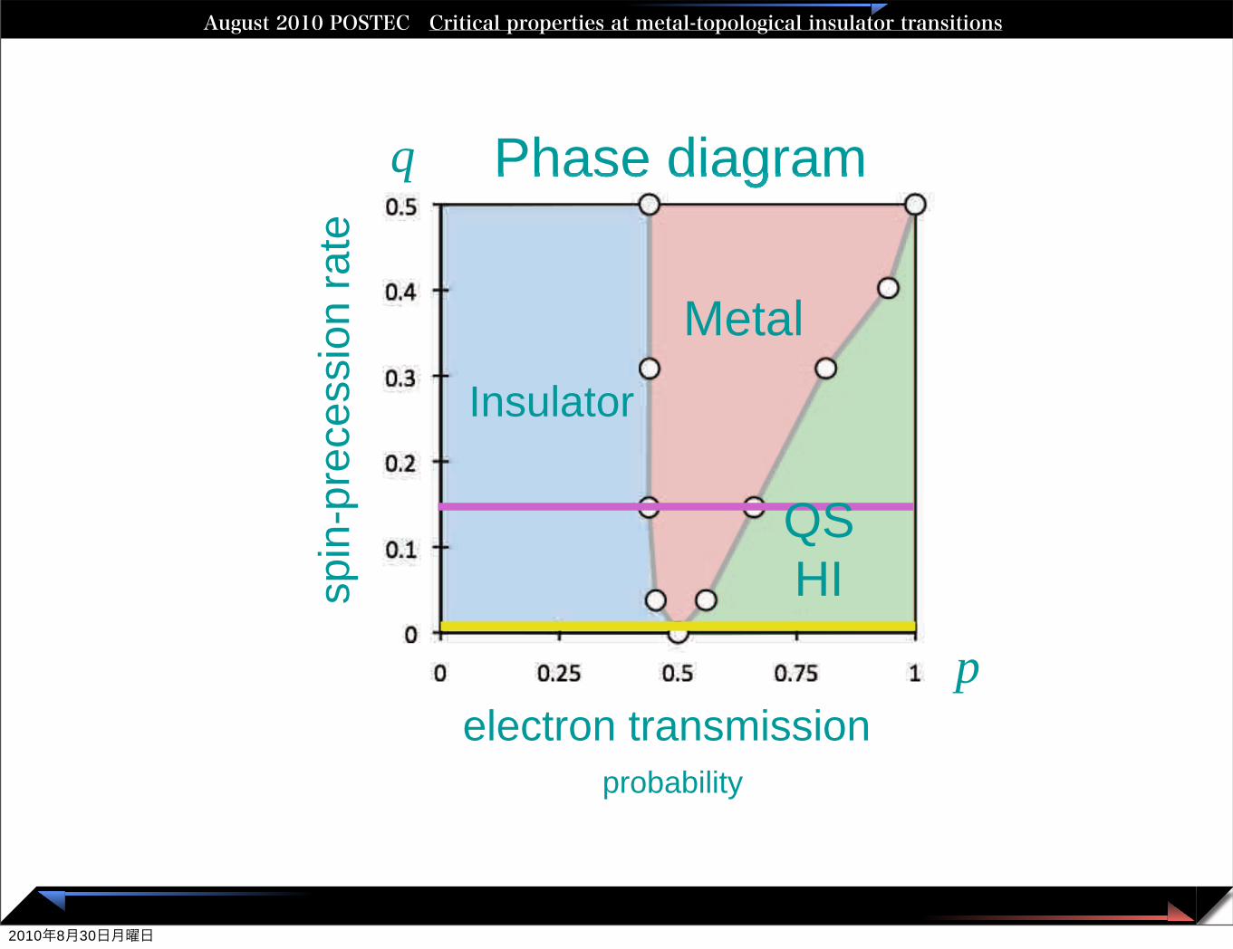
FIG. 2: (Color online) Phase diagram for the network modelafter Ref. 11.
Kramers doublets that preserves TRS but can break SRS.When r = 1 and t = 0, S is reduced to the unit ma-trix, and there is no tunneling between one Kramers pair("1 + "2) and the other pair ("3 + "4). The tunnel-ing with (without) a spin flip occurs with the probabilityt2 sin2 # (t2 cos2 #). Although S is parametrized by fourreal parameters, only X and # matter as $1 and $2 can beabsorbed in the overall phase windings that the Kramersdoublets acquire when traversing along links connectingnodes.
Disorder is introduced in the network model by assum-ing that the phases of Kramers doublets on the links andthe phases # on the nodes are independently and iden-tically distributed. The distribution of the link phase ofa Kramers doublet is uniform over the interval [0, 2%[.The distribution of # is sin 2# over the interval [0, %/2].We are left with one parameter X in the network modelthat controls the scattering amplitude at every nodes.The parameter # in the network model plays the samerole as spin-orbit interactions (of Rashba type) in a ran-dom tight-binding Hamiltonian belonging to the two-dimensional symplectic symmetry class, whereas the pa-rameter X plays the role of the Fermi energy.
In order to distinguish the topologically-trivial insulat-ing phase from the QSH insulating phase, we shall com-pare the results that we obtained from the network modelagainst the ones that we obtained from a two-dimensionaltight-binding model introduced in Ref. 2, the so-calledSU(2) model. The SU(2) model is a microscopic randomtight-binding Hamiltonian with on-site randomness (boxdistributed with the width W ) and with random hop-ping amplitudes such that the spin-dependent hoppingamplitudes between any pair of nearest-neighbor sitesof a square lattice are distributed so as to generate theSU(2) invariant Haar measure. It captures the transitionbetween a metallic and a topologically-trivial insulatingstate in the ordinary two-dimensional symplectic univer-sality class. In the SU(2) model, the Fermi energy playsthe role of the network parameter X for a fixed and nottoo strong W .
III. PHASE DIAGRAM AND BOUNDARYCONDITIONS
On symmetry grounds, we expect that it is possible todrive the network model through two successive Ander-son transitions by tuning X . Indeed, this was shown to bethe case in Ref. 11. For any X bounded by the two criticalvalues Xs < Xl [Xs = 0.047±0.001, Xl = 0.971±0.001;the subscript s (l) stands for small (large)] the network
2
FIG. 1: (Color online) Elementary building blocks of the net-work model. A square Bravais lattice with nearest-neighborsites connected by bonds underlies the construction of thenetwork model. Any red site of one of the two sublattices ofthe square lattice is replaced by a red circle S (a node of typeS) with the four bonds meeting at the site replaced by fourpairs of directed links numbered according to the rule shownin (a). Any blue site of the complementary sublattice of thesquare lattice is replaced by a blue circle S
! (a node of typeS!) with the four bonds meeting at the site replaced by four
pairs of directed links numbered according to the rule shownin (b). Observe that a clockwise rotation by !/2 turn (a) into(b). The directed links represent incoming or outgoing planewaves with a well-defined projection of the spin-1/2 quantumnumber along the quantization axis. Each pair of links re-placing a bond represents a Kramers doublet of plane waves.Each node S or S
! depicts a scattering process represented bya 4!4 unitary matrix defined in Eq. (2.1) that preserves time-reversal symmetry (TRS) but breaks spin-rotation symmetry(SRS).
tum number ! =!. A link represented by a dashed linecarries the spin-1/2 quantum number ! =". Third, thefour pairs of directed links that meet at a node are la-beled according to the rules of Fig. 1(a) and Fig. 1(b)if the node is of type S and S
!, respectively. With theconventions of Figs. 1(a) and 1(b) either node defines a4# 4 scattering matrix S that preserves TRS but breaksthe SRS and can be represented by
!
"
"
"
"
#
"(o)1"
"(o)2#
"(o)3"
"(o)4#
$
%
%
%
%
&
= S
!
"
"
"
"
#
"(i)2"
"(i)1#
"(i)4"
"(i)3#
$
%
%
%
%
&
, S =
'
r!0 tQ$tQ† r!0
(
,
r = tanhX, t =1
coshX,
Q = i!0 cos # sin$1 + !1 sin # cos$2
$ !2 sin # sin$2 + !3 cos # cos$1.
(2.1)
Here, the four matrices !0,1,2,3 act on the spin-1/2 com-ponents with !0 the unit 2#2 matrix and ! = (!1, !2, !3)the three Pauli matrices. Moreover, 0 % X < &,0 % # < %/2, 0 % $1 < 2%, and 0 % $2 < 2%. TRSis represented by the condition
S =
'
!2 00 !2
(
ST
'
!2 00 !2
(
. (2.2)
The matrix S is the most general 4 # 4 unitary matrixthat describes a quantum tunneling process between two
FIG. 2: (Color online) Phase diagram for the network modelafter Ref. 11.
Kramers doublets that preserves TRS but can break SRS.When r = 1 and t = 0, S is reduced to the unit ma-trix, and there is no tunneling between one Kramers pair("1 + "2) and the other pair ("3 + "4). The tunnel-ing with (without) a spin flip occurs with the probabilityt2 sin2 # (t2 cos2 #). Although S is parametrized by fourreal parameters, only X and # matter as $1 and $2 can beabsorbed in the overall phase windings that the Kramersdoublets acquire when traversing along links connectingnodes.
Disorder is introduced in the network model by assum-ing that the phases of Kramers doublets on the links andthe phases # on the nodes are independently and iden-tically distributed. The distribution of the link phase ofa Kramers doublet is uniform over the interval [0, 2%[.The distribution of # is sin 2# over the interval [0, %/2].We are left with one parameter X in the network modelthat controls the scattering amplitude at every nodes.The parameter # in the network model plays the samerole as spin-orbit interactions (of Rashba type) in a ran-dom tight-binding Hamiltonian belonging to the two-dimensional symplectic symmetry class, whereas the pa-rameter X plays the role of the Fermi energy.
In order to distinguish the topologically-trivial insulat-ing phase from the QSH insulating phase, we shall com-pare the results that we obtained from the network modelagainst the ones that we obtained from a two-dimensionaltight-binding model introduced in Ref. 2, the so-calledSU(2) model. The SU(2) model is a microscopic randomtight-binding Hamiltonian with on-site randomness (boxdistributed with the width W ) and with random hop-ping amplitudes such that the spin-dependent hoppingamplitudes between any pair of nearest-neighbor sitesof a square lattice are distributed so as to generate theSU(2) invariant Haar measure. It captures the transitionbetween a metallic and a topologically-trivial insulatingstate in the ordinary two-dimensional symplectic univer-sality class. In the SU(2) model, the Fermi energy playsthe role of the network parameter X for a fixed and nottoo strong W .
III. PHASE DIAGRAM AND BOUNDARYCONDITIONS
On symmetry grounds, we expect that it is possible todrive the network model through two successive Ander-son transitions by tuning X . Indeed, this was shown to bethe case in Ref. 11. For any X bounded by the two criticalvalues Xs < Xl [Xs = 0.047±0.001, Xl = 0.971±0.001;the subscript s (l) stands for small (large)] the network
t2 = 1t2 = 0 t2 = 0.5
scattering matrix
2010年8月30日月曜日
Critical conductance distributions at the localization-delocalization transitionsAugust 2010 POSTEC Critical properties at metal-topological insulator transitions
Phase diagram Phase diagram
electron transmission probability
spin
-pre
cess
ion
rate
p
q
QSHI
Insulator
Metal
2010年8月30日月曜日
Critical conductance distributions at the localization-delocalization transitionsAugust 2010 POSTEC Critical properties at metal-topological insulator transitions
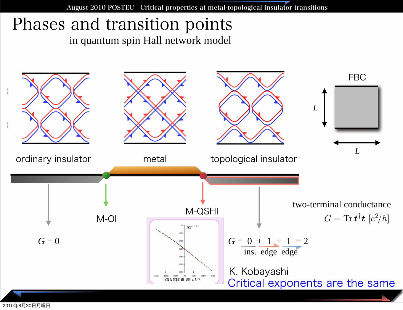
Phases and transition points
L
L
FBC
G = 0 G = 0 + 1 + 1 = 2
in quantum spin Hall network model
metalordinary insulator topological insulator
two-terminal conductanceM-OI
M-QSHI
ins. edge edgeins. edge edge = 0 + 1 + 1 = 2
s =!
ei!2 00 ei!4
"!r tt !r
"!ei!1 00 ei!3
". (8)
#!R
$=
Nx%
i=1
T (i)#!L
$, !R = T (M) · · ·T (2)T (1) !L !out = S !in (9)
G =h
e2g = Tr t†t G = Tr t†t [e2/h]
G ! G! = Tr t†t ! Tr t!†t! (10)= Tr (t†t!r†r) ! Tr (t!†t!r!†r!) (11)= Tr I(N+1)"(N+1) ! Tr IN"N (12)= 1 (13)
G > 1 (14)
t(N+1)"(N+1) = U
&
''''''(
"1 0 · · · 0
0 "2
......
. . ."N 0
0 · · · 0 1
)
******+V (15)
0.1 Perfectly conducting channel in unitary class
In the unitary case, a PCC arises from the asymmetry of the number of the incomingand outgoing channels [?]. On the left side, the network has N + 1 incoming and N
outgoing channels. Hence the reflection matrix r has the dimension (N + 1) " N .Because
rank (r†r)(N+1)"(N+1) = rank rN"(N+1) # N, (16)
there is at least one reflection eigenvalue ‘0’. That implies the existence of a PCC.
0.2 Perfectly conducting channel in symplectic class
In the symplectic case, a PCC arises from the odd number of the dimension of thereflection matrices. The symplectic symmetry requires that
S = !ST. (17)
Then it follows thatr = !rT, (18)
and by taking its determinant,
det(r) = det(!rT) = (!1)2N+1 det(r) = 0. (19)
Thereforerank r(2N+1)"(2N+1) # 2N. (20)
Thus r has at least one eigenvalue ‘0’ and there exists a PCC.
#� $" !#%� #!" � #&� $� � %� � � � #$! � #� $� &! $� � � � � $!#� � #� � � ( � %( � � � " � 3� � � � � � +$%� � $�
� 2� � ! � � +� $� � 7 0� 2� � � %$( � � 7 0� � 2� � � ( $� 8� � � � � 2� � � � ) � 9� �
� � 0+� 8� � 0*0+�# "8� � 408� 0� *4� =FDDK >� � � � � =<� DK IGDE�
E� � ( �* ,% � & , � ' � � � !4+"� +8� � ' (!"�� � & "1 � *+",48� � F � � ( �* ,% � & , � ' � � � !4+"� +8� � 4' , ' � � & "1 � *+",48� � G� � ( �* ,% � & , � ' � � � !4+"� +8� � +�# �� � & "1 � *+",4�
) 0�& -5 � � � +("& <� 0**� & , �
"& +0$� , ' *�
� � � � +, � , � �
� � � � +, � , � �
���%��$����/�
� � *& � 1 " 8� � !�& � =FDDJ>� � � � � ?<� EDJ L DF� �
� �& � 8� � $� � =FDDI>� � � � � ?;� EHJ L DF�
•!� � ' <& ' *% �$ � � "+,*"� 0-' & � � ' *� � �
•!� � � � � � � � � � � � � � � � � � � � � � � � � � � � � ' *� � � � �•!� � � � � � � � � ' & 1 � * � � , ' � � "� � *� & , � 1 �$ 0� +
� +-% � , � � � � � � *' % � ,!� �
+� � ' & � <+% �$ $� +, � (' +"-1 � � � � �
��$(�%�=,2
'<,�*%
"&�$��'&�0�,�&��>�
��$(�%�=�*"-��$
��3('&�&,>�
<� � *"-� �$ � � 3(' & � & , � � � � �
' � � � "1 � * � & � � � ' � � ,!� � $' � �$ "5 � -' & � $� & ,!�
<� � *"-� �$ � � "+,*"� 0-' & � � 0& � -' & � P(G) ' � � , 2 ' <, � *% "& �$ � � ' & � 0� , �& � � � G
� !�+ � � � "� *�% �
� , �$ $"� � (!�+ � �
: random phase
� 0% � *"� �$ � � �$ � 0$� -' & � ' � � , *�& +(' *, � (*' ( � *-� +�
"& � � "+' *� � *� � � ) 0�& ,0% � +("& < �$ $� =� � >� +4+, � % +�
� %#!�(�&! �
� ("& <*' , � -' & � +4% % � ,*49� � � �
•!� � �0 ++"� & � � "+,*"� 0-' & �
•!� � 1 � *� � � ' � �
�! ��($�! �
•!� � *"-� �$ � � ' & � 0� , �& � � � � "+,*"� 0-' & +� �
� *"-� �$ � � ' & � 0� , �& � � � � "+,*"� 0-' & +� � � ( � & � � �$ +' � ' & � �
%� � � � � � � � $%� %� $� � � %� � � � � � � � � %� � $( � � & � � " � � $� :� �
•!� � ' "& � "� � � 2 ",!� � ' & 1 � & -' & �$ � +4% ($� � -� � +4+, � % +�
� ' & +"+, � & , � 2 ",!� ,!� � � ' & 1 � & -' & �$ � +4% ($� � -� � +4+, � % +�
� +�� �� � , � � $:� =FDDH>� � � � � =6� DGIEEI� �
2 ",!' 0, � � � � � =� � � >�
2 ",!� � � � �
� �% � � �+ � � ' & 1 � & -' & �$ � +4% ($� � -� � % � , � $+�
� "% � <*� 1 � *+�$ � +4% % � ,*49� � � � �@� M� $+� " � � � & � � � � � $$�
& +0$� -& � (!�+ � +�
� MFIJ �
+4+, � % � +"5 � � � MJH�
� MEFL �
� � � "& +0$� , ' *�
' *� "& �* 4� "& +0$� , ' *�
����#� ��1��#��)1766=2:6=9�
� �� � � �
� � � , � $<� � � "& +0$� , ' *� , *�& +"-' & �
' � � ?�
•!� � *"-� �$ � � 3(' & � & , � ' � � $' � �$ "5 � -' & � $� & ,!�
( � � 0$"�* � +!�( � � � ' *� <� � � , *�& +"-' & � �
� � � +4+, � % �
� ' & 1 � & -' & �$ � F � � +4% ($� � -� � +4+, � % �
� ' & +"+, � & , � 2 ",!� � ' & 1 � & -' & �$ �
+4% ($� � -� � +4+, � % +�
0& "1 � *+�$ � +!�( � � � ' *� <� � , *�& +"-' & � � � �
� *"-� �$ � � 3(' & � & , � ' � � $' � �$ "5 � -' & � $� & ,!�
� ' � +� !%� � � ( � & � � ' & � ,!� � � � � � +, � , � +:�
� 8� � %* !#� � � ! � � � �
� 0�& ,0% � +("& < �$ $� "& +0$�, ' *�
& 1 � +- � -' & � ' � � ,!� � ( � ) � #$� � � " #!" � #&� $�
� , � � & � � *+' & � , *�& +"-' & +� ' � � � � � +4+, � % +�
� !� � $' � �$ "5 � -' & � $� & ,!�
"+� , ' ' � $�* � :� �
=� � � � 0+� � ' � � ,!� � � � � � +, � , � +>�
� � � � � � � � � � � � ( � %+�
M� "& 1 � *+� � ' � � ,!� � +% �$ $� +, � (' +"-1 � �
� 4� (0& ' 1 � � 3(' & � & , � =� � >�
<� � � , *�& +"-' & �� �
� � 0+� � � , � � $:� =FDDL >� � � � � => 8� EEIGDE�
� � <� � , *�& +"-' & �
� *� � ,!� � � *"-� �$ � (*' ( � *-� +� � "� � *� & , � � *' % �
� ' & 1 � & -' & �$ � F � � +4% ($� � -� � +4+, � % +7�
� �
� �
� 0*(' +� �
•!� � � ( � & � � ' & � ,!� � $+� � � %#+�
•!� � ' � !%� � � ( � & � � ' & � ,!� � $+$%� � � $� ,� 8� � ! � � � 8� �
�& � � % "� *' +� ' ("� � ( �* �% � , � *+�
� & "1 � *+�$ � (*' ( � *-� +�
+4+, � % � +"5 � � +4+, � % � +"5 � �
� � � +4+, � % 9�
=& � , 2 ' *#� % ' � � $� �& � � - !, �
� "& � "& � % ' � � $8� *� +( � � -1 � $48� �
� ' *� � ' & 1 � & -' & �$ � +4% ($� � -� �
+4+, � % +>�
•!� � "� � *� & , � � *' % � <� � , *�& +"-' & �
"& � � ( � & � � & , � ' � �
� ;�
� �
� ;�
� � =F>� % ' � � $�
� F � % ' � � $�
� F � � � % ' � � $�
� ;�
� "% "-& � 1 �$ 0� +� *� � � � , � ,!� � � � � � +, � , � +�
� ! � " � � %� � +� � � � � #� %.�
•!� +4+, � % � +"5 � �
•!� % ' � � $� ( � *�% � , � *�
� 3( � � , � � � , ' � � � � 0& "1 � *+�$ �
+� � /� *"& � % � , *"3�
� � � � FDEDA � ' #4' � � & "1:� � � FDED:L :G�
� � :� � 0�& ,0% � �$ $� "& +0$�, ' *�
!" !� !� � � � � � � $( � � %!#$�
•!� � � � � +, � , � �•!� ) 0� & -5 � � � � ' & � 0� , �& � � �
•!� � !� *�� , � *"5 � � � � 4�
, ' (' $' "� �$ � & 0% � � *�
<� � � � "& +0$�, ' *9� � F �<� � � "& +0$�, ' *9� � !
� , � $<' *� "& �* 4� "& +0$� , ' *� , *�& +"-' & �
� MFIJ � � MEFL �
� � � "& +0$� , ' *�
' *� "& �* 4� "& +0$� , ' *�
� � �
� � �
� � � �
� � � �
� � �
� � � �
� �
� � � � � � � � � � � � � � � � � � � � � � � � � � �
uL1/!+� �$ "& � 1 �* "�� $� �
!2corrected
K. KobayashiCritical exponents are the same
2010年8月30日月曜日
Critical conductance distributions at the localization-delocalization transitionsAugust 2010 POSTEC Critical properties at metal-topological insulator transitions
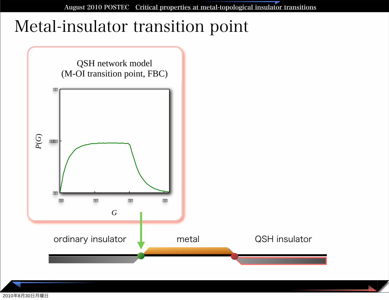
Metal-insulator transition point
� �
� � � �
� �
� � � � � � � �
G
P(G
)
QSH network model (M-OI transition point, FBC)
metalordinary insulator QSH insulator
2010年8月30日月曜日
Critical conductance distributions at the localization-delocalization transitionsAugust 2010 POSTEC Critical properties at metal-topological insulator transitions
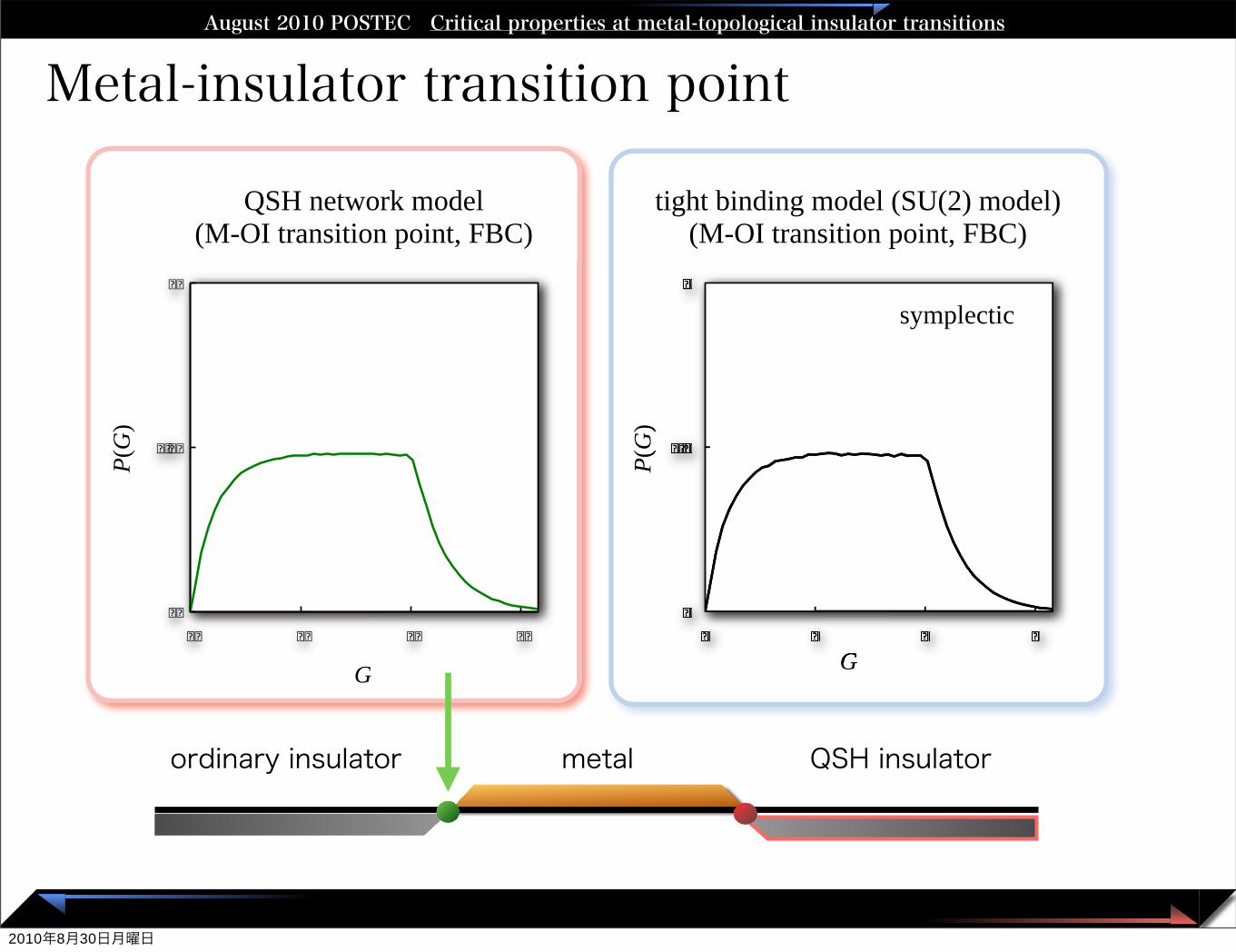
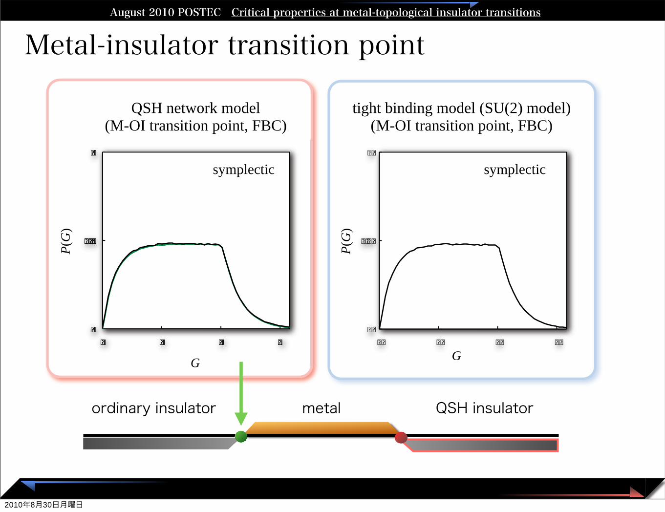
Metal-insulator transition point
� �
� � � �
� �
� � � � � � � �
G
P(G
)
QSH network model (M-OI transition point, FBC)
metalordinary insulator QSH insulator
� �
� � � �
� �
� � � � � � � �
tight binding model (SU(2) model)(M-OI transition point, FBC)
GP(
G)
symplectic
� �
� � � �
� �
� � � � � � � �
G(
)
symplectic
2010年8月30日月曜日
Critical conductance distributions at the localization-delocalization transitionsAugust 2010 POSTEC Critical properties at metal-topological insulator transitions
Metal-insulator transition point
� �
� � � �
� �
� � � � � � � �
G
P(G
)
QSH network model (M-OI transition point, FBC)
symplectic
metalordinary insulator QSH insulator
� �
� � � �
� �
� � � � � � � �
tight binding model (SU(2) model)(M-OI transition point, FBC)
GP(
G)
symplectic
� �
� � � �
� �
� � � � � � � �
symplectic
2010年8月30日月曜日
Critical conductance distributions at the localization-delocalization transitionsAugust 2010 POSTEC Critical properties at metal-topological insulator transitions
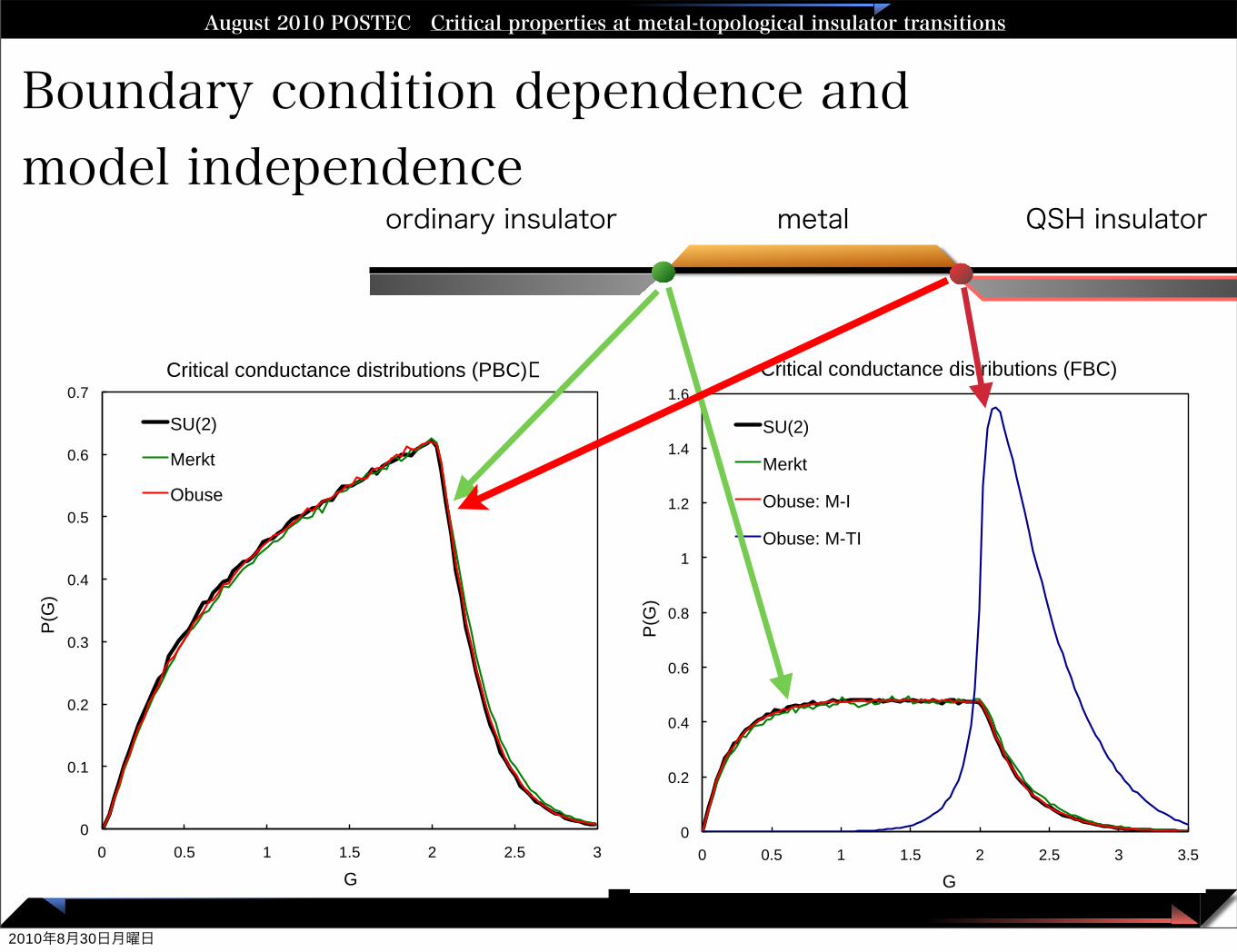
Boundary condition dependence and model independence
0
0.1
0.2
0.3
0.4
0.5
0.6
0.7
0 0.5 1 1.5 2 2.5 3
P(G
)
G
Critical conductance distributions (PBC) �
SU(2)
Merkt
Obuse
0
0.2
0.4
0.6
0.8
1
1.2
1.4
1.6
0 0.5 1 1.5 2 2.5 3 3.5
P(G
)
G
Critical conductance distributions (FBC)
SU(2)
Merkt
Obuse: M-I
Obuse: M-TI
metalordinary insulator QSH insulator
2010年8月30日月曜日
Critical conductance distributions at the localization-delocalization transitionsAugust 2010 POSTEC Critical properties at metal-topological insulator transitions
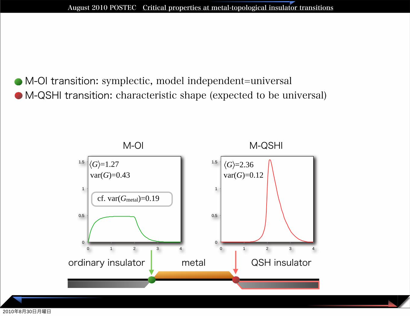
M-OI transition: symplectic, model independent=universalM-QSHI transition: characteristic shape (expected to be universal)
0
0.5
1
1.5
0 1 2 3 4 0
0.5
1
1.5
0 1 2 3 4
〈G〉=1.27 〈G〉=2.36var(G)=0.43 var(G)=0.12
cf. var(Gmetal)=0.19
metalordinary insulator QSH insulator
M-QSHIM-OI
2010年8月30日月曜日
Critical conductance distributions at the localization-delocalization transitionsAugust 2010 POSTEC Critical properties at metal-topological insulator transitions
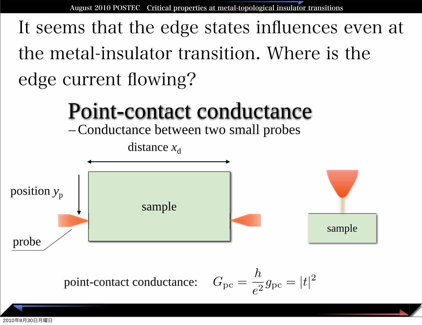
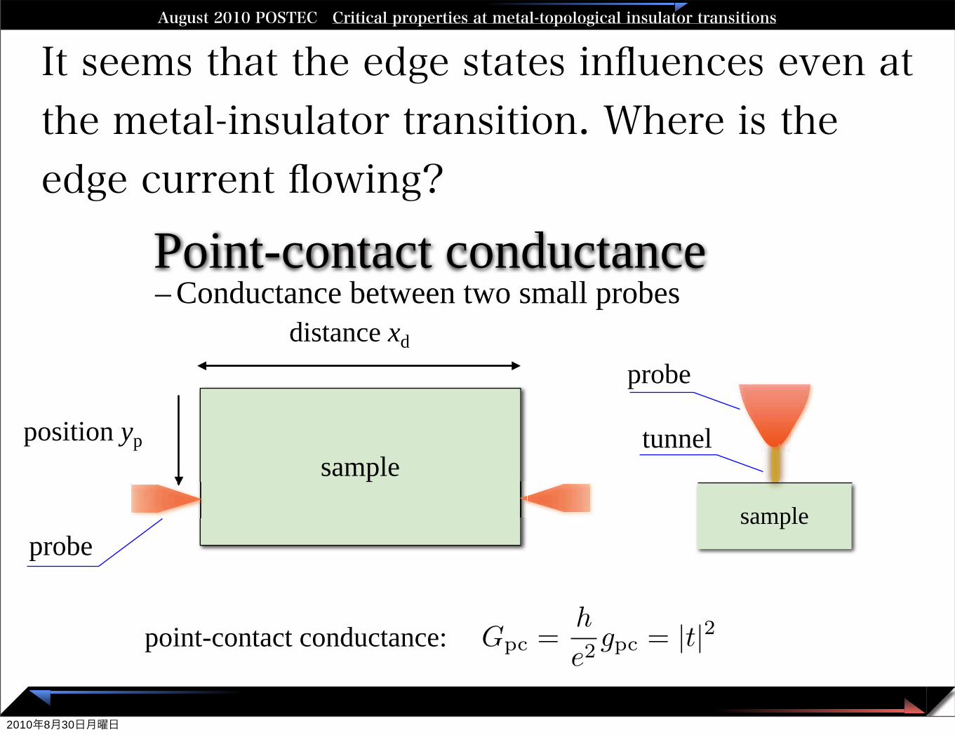
It seems that the edge states influences even at the metal-insulator transition. Where is the edge current flowing?
Gpc =h
e2gpc = |t|2
Point-contact conductance– Conductance between two small probes
distance xd
position ypsample
probe
point-contact conductance:
sample
2010年8月30日月曜日
Critical conductance distributions at the localization-delocalization transitionsAugust 2010 POSTEC Critical properties at metal-topological insulator transitions
It seems that the edge states influences even at the metal-insulator transition. Where is the edge current flowing?
Gpc =h
e2gpc = |t|2
Point-contact conductance– Conductance between two small probes
distance xd
position ypsample
probe
point-contact conductance:
sample
probe
tunnel
2010年8月30日月曜日
Critical conductance distributions at the localization-delocalization transitionsAugust 2010 POSTEC Critical properties at metal-topological insulator transitions
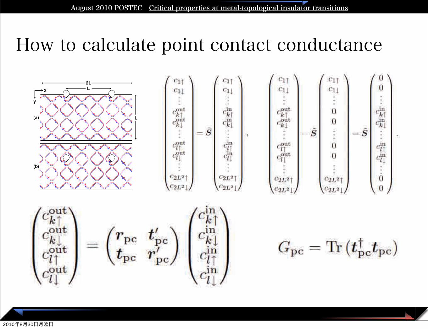
How to calculate point contact conductance
6
FIG. 11: (Color online) Distribution functions of the largestP (2!1) (—–) and second-largest P (2!3) (- - -) transmissioneigenvalues for M-QSHI transition D. Dotted lines are thedistribution functions of the conductance P (G) in Fig. 9 forG < 2 and for G > 2, both of which are normalized to be1. The latter is shifted by !2 along the horizontal axis to becompared with P (2!3).
FIG. 12: (Color online) Schematics of the Z2 networks withpoint contacts on the edge, yp = 1 (a), and in the bulk region,yp = L/2 (b). Each point contact is connected with a link.PBC are imposed on the longitudinal direction.
tunneling microscope tips). For the network model, thepoint-contact conductance is calculated as the conduc-tance between two links.25–27 We consider a cylindricalgeometry (2L links in the x-direction and L links in they-direction) and two point contacts separated by distanceL as shown in Fig. 12. The point-contact conductancedepends on the position of the contacts in the y-direction.We assume that both contacts are located at the samedistance from one of the edges. That is, the contacts areattached at (x, y) = (0, yp) and (L, yp).
B. Method
To introduce point contacts into the network, we cutlink k and link l where the contacts are attached. Wethen define incoming current amplitudes (cin
k!, cink", c
inl!, c
inl")
and outgoing current amplitudes (coutk! , cout
k" , coutl! , cout
l" ) onthe corresponding links. The current amplitudes satisfythe equation
!
"""""""""""""""""#
c1!c1"...
coutk!
coutk"...
coutl!
coutl"...
c2L2!c2L2"
$
%%%%%%%%%%%%%%%%%&
= S̃
!
"""""""""""""""""#
c1!c1"...
cink!
cink"...
cinl!
cinl"...
c2L2!c2L2"
$
%%%%%%%%%%%%%%%%%&
, (13)
where the 4L2 ! 4L2 scattering matrix S̃ for all linksof a network consists of the 4 ! 4 scattering matri-ces si and s#
i in Eqs. (1) - (4) for a node. Forgiven (cin
k!, cink", c
inl!, c
inl"), the remaining current amplitudes
(c1!, · · · , coutk! , cout
k" , · · · , coutl! , cout
l" , · · · , c2L2") are uniquelydetermined by the following set of 4L2 simultaneous lin-ear equation with 4L2 unknowns
!
"""""""""""""""""#
c1!c1"...
coutk!
coutk"...
coutl!
coutl"...
c2L2!c2L2"
$
%%%%%%%%%%%%%%%%%&
" S̃
!
"""""""""""""""""#
c1!c1"...
00...
00...
c2L2!c2L2"
$
%%%%%%%%%%%%%%%%%&
= S̃
!
"""""""""""""""""#
00...
cink!
cink"...
cinl!
cinl"...00
$
%%%%%%%%%%%%%%%%%&
. (14)
As a consequence of the structure of these equations,there is a linear relationship between the incoming andoutgoing current amplitudes
!
""#
coutk!
coutk"
coutl!
coutl"
$
%%& ='
rpc t#pc
tpc r#pc
(!
""#
cink!
cink"
cinl!
cinl"
$
%%& . (15)
The point-contact conductance Gpc is given by
Gpc = Tr (t†pctpc), (16)
in units of e2/h.
2010年8月30日月曜日
Critical conductance distributions at the localization-delocalization transitionsAugust 2010 POSTEC Critical properties at metal-topological insulator transitions
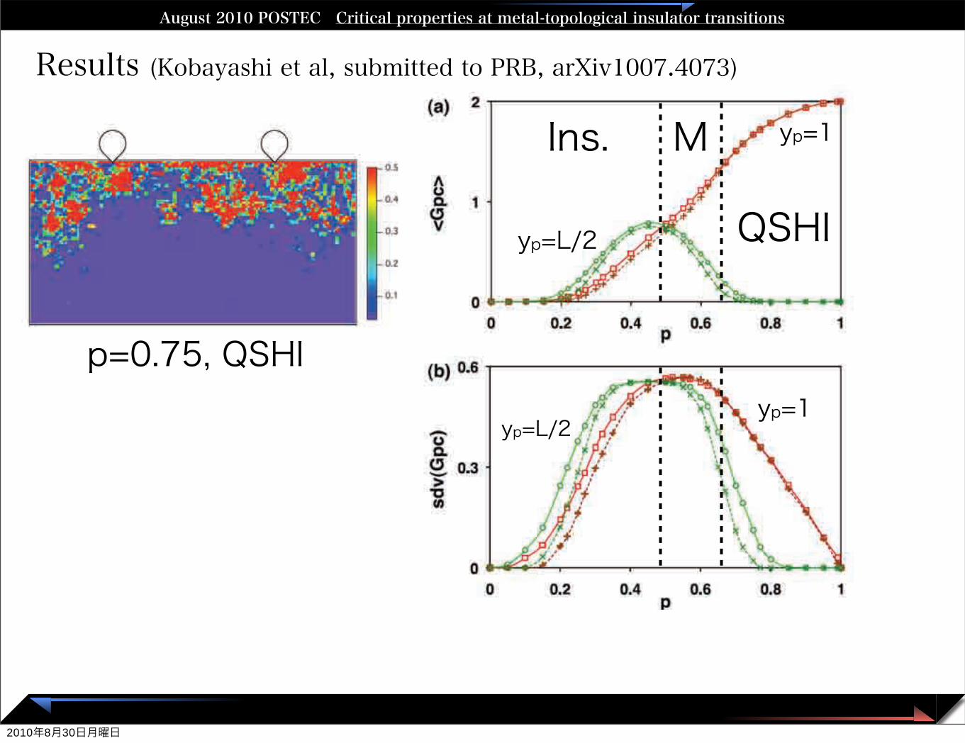
Results (Kobayashi et al, submitted to PRB, arXiv1007.4073)
yp=1
yp=L/2
yp=1yp=L/2
p=0.75, QSHI
Ins. M
QSHI
2010年8月30日月曜日
Critical conductance distributions at the localization-delocalization transitionsAugust 2010 POSTEC Critical properties at metal-topological insulator transitions
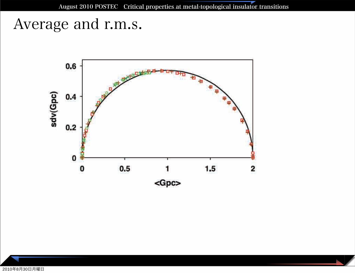
Average and r.m.s.
2010年8月30日月曜日
Critical conductance distributions at the localization-delocalization transitionsAugust 2010 POSTEC Critical properties at metal-topological insulator transitions
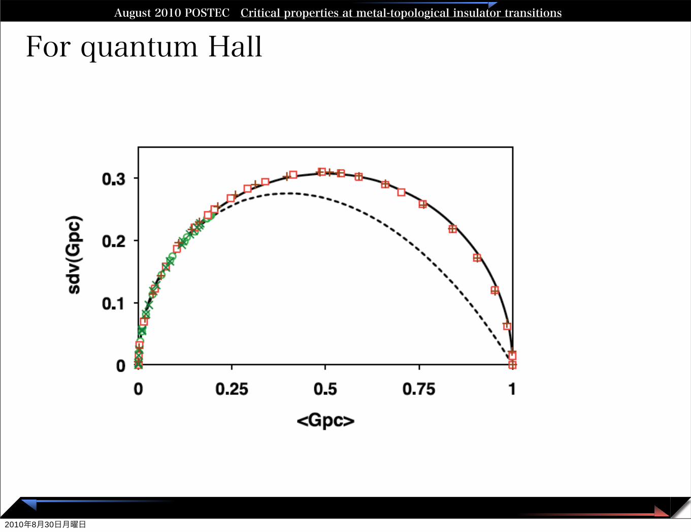
For quantum Hall
2010年8月30日月曜日
August 2010 POSTEC Critical properties at metal-topological insulator transitions
Summary• p(g) at the Anderson transition
–independent of models, sizes–sensitive to the number of edge states in the adjacent
insulating phase• Quantum Hall transition (Z toplogical insulator)
– sensitive to the Landau level indices• Symplectic (Z2 topological insulator)
– for ordinary metal-insulator transition, very good agreement between the tight binding SU(2) and the network model
– peculiar p(g) at the quantum spin Hall transition, again sensitive to the number of edge states
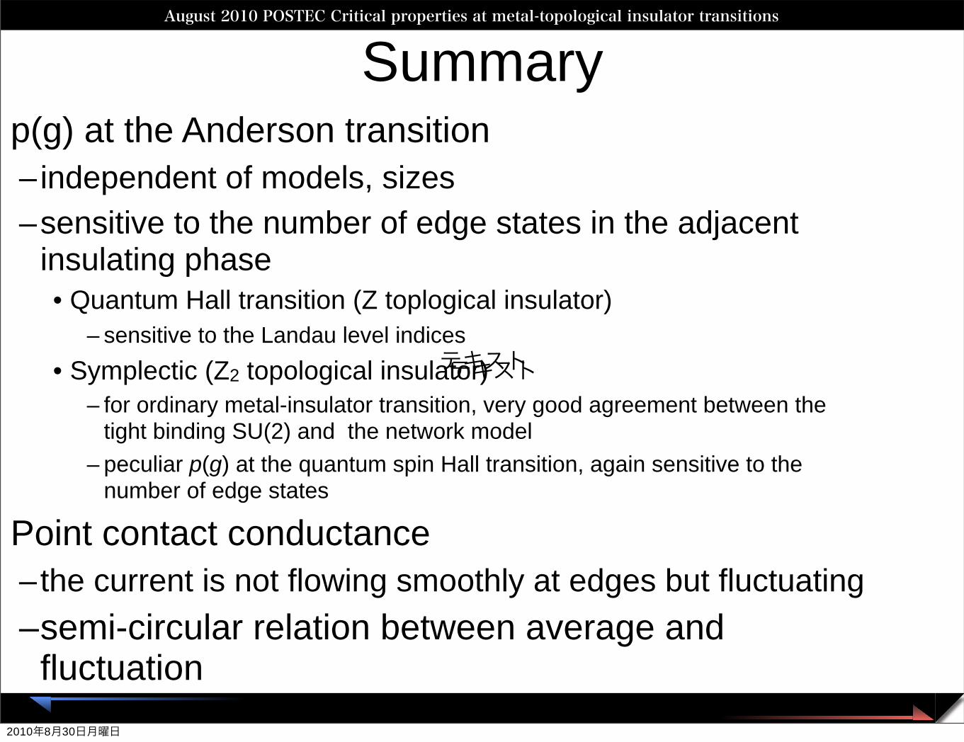
• Point contact conductance–the current is not flowing smoothly at edges but fluctuating–semi-circular relation between average and
fluctuation
テキストテキスト
2010年8月30日月曜日


![Topological, Valleytronic, and Optical Properties of Monolayer PbS · PDF file · 2017-03-30Topological, Valleytronic, and Optical Properties of Monolayer PbS ... (PbS) [1] is an](https://img.pdfslide.tips/doc/110x75/5aa374327f8b9a84398e5cc5/topological-valleytronic-and-optical-properties-of-monolayer-pbs-valleytronic.jpg)