Embed Size (px)
DESCRIPTION
Anna Univ EIE notes
Citation preview
DEPARTMENT OF COMPUTER SCIENCE AND ENGINEERING
SEMESTER -VII
LECTURE NOTES
ON
CS2023 – OPERATING SYSTEMS
PREPARED BY
MR.RAJKUMAR.S
AP/CSE
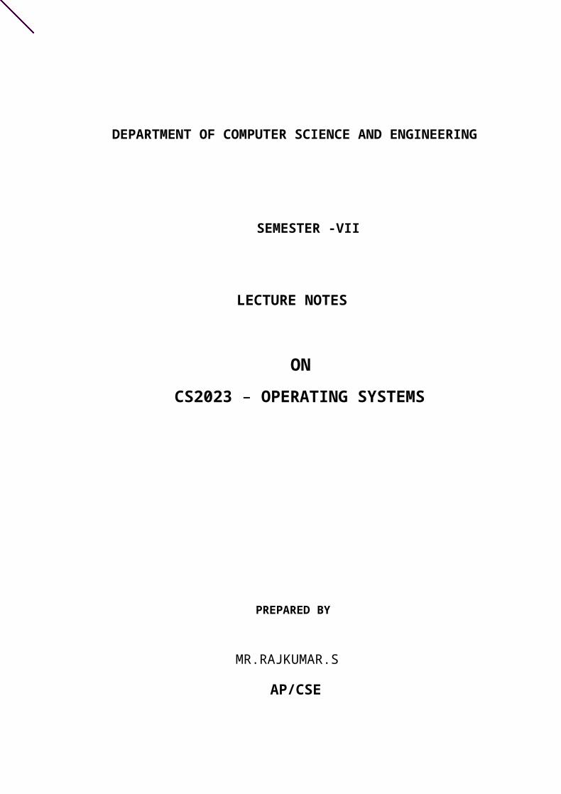
SYLLABUS CS2254 – OPERATING SYSTEMS
UNIT I PROCESSES AND THREADS
Introduction to operating systems – Review of computer organization – Operating system structures – System calls – System programs – System structure – Virtual machines – Processes – Process concept – Process scheduling – Operations on processes – Cooperating processes – Inter process communication – Communication in client – Server systems – Case study – IPC in Linux – Threads – Multi-threading models – Threading issues – Case Study: Pthreads library
UNIT II PROCESS SCHEDULING AND SYNCHRONIZATION
CPU scheduling – Scheduling criteria – Scheduling algorithms – Multiple – Processor scheduling – Real time scheduling – Algorithm evaluation – Case study – Process scheduling in Linux – Process synchronization – The critical-section problem – Synchronization hardware – Semaphores – Classic problems of synchronization – Critical regions – Monitors – Deadlock – System model – Deadlock characterization – Methods for handling deadlocks – Deadlock prevention – Deadlock avoidance – Deadlock detection – Recovery from deadlock.
UNIT III STORAGE MANAGEMENT
Memory management – Background – Swapping – Contiguous memory allocation – Paging – Segmentation – Segmentation with paging – Virtual memory – Background – Demand paging – Process creation – Page replacement – Allocation of frames – Thrashing – Case study – Memory management in Linux . UNIT IV FILE SYSTEMS
File system interface – File concept – Access methods – Directory structure – File system mounting – Protection – File system implementation – Directory implementation – Allocation methods – Free space management – Efficiency and performance – Recovery – Log-structured file systems – Case studies – File system in Linux – File system in Windows XP.
UNIT V I/O SYSTEMS
I/O systems – I/O hardware – Application I/O interface – Kernel I/O subsystem – Streams – Performance – Mass-storage structure – Disk scheduling – Disk management – Swap-space management – RAID – Disk attachment – Stable storage – Tertiary storage – Case study – I/O in Linux.
TEXT BOOKS
1. Silberschatz, Galvin, and Gagne, “Operating System Concepts”, Sixth Edition, Wiley India Pvt Ltd, 2003.
REFERENCES:
1. Andrew S. Tanenbaum, “Modern Operating Systems”, Second Edition, Pearson Education, 2004. 2. Gary Nutt, “Operating Systems”, Third Edition, Pearson Education, 2004. 3. Harvey M. Deital, “Operating Systems”, Third Edition, Pearson Education, 2004.
UNIT I PROCESSES AND THREADS
Introduction to operating systems – Review of computer organization – Operating system structures – System calls– System programs – System structure – Virtual machines – Processes – Process concept – Process scheduling –Operations on processes – Cooperating processes – Inter process communication – Communication in client – Server systems – Case study – IPC in linux – Threads – Multi-threading models – Threading issues – Casestudy – Pthreads library.
UNIT 1
What is an Operating System?
A program that acts as an intermediary between a user of a computer and the computer hardware.
Operating system goals:
Execute user programs and make solving user problems easier.
Make the computer system convenient to use.
Use the computer hardware in an efficient manner.
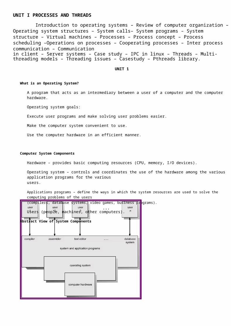
Computer System Components
Hardware – provides basic computing resources (CPU, memory, I/O devices).
Operating system – controls and coordinates the use of the hardware among the various application programs for the various users.
Applications programs – define the ways in which the system resources are used to solve the computing problems of the users
(compilers, database systems, video games, business programs).
Users (people, machines, other computers).
Abstract View of System Components
Operating System Definitions
Resource allocator – manages and allocates resources.
Control program – controls the execution of user programs and operations of I/O devices .
Kernel – the one program running at all times (all else being application programs).
Mainframe Systems
Reduce setup time by batching similar jobs Automatic job sequencing – automatically transfers control from one job to another. First rudimentary operating system. Resident monitor
initial control in monitor control transfers to job when job completes control transfers pack to monitor
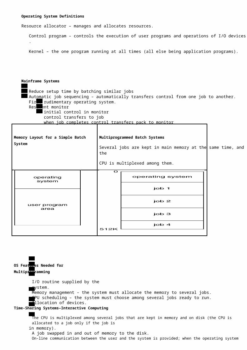
Memory Layout for a Simple Batch System
OS Features Needed for Multiprogramming
I/O routine supplied by the system.
Multiprogrammed Batch Systems
Several jobs are kept in main memory at the same time, and the
CPU is multiplexed among them.
Memory management – the system must allocate the memory to several jobs. CPU scheduling – the system must choose among several jobs ready to run. Allocation of devices.
Time-Sharing Systems–Interactive Computing
The CPU is multiplexed among several jobs that are kept in memory and on disk (the CPU is allocated to a job only if the job is in memory).
A job swapped in and out of memory to the disk. On-line communication between the user and the system is provided; when the operating system finishes the execution of
one command, it seeks the next “control statement” from the user’s keyboard On-line system must be available for users to access data and code.
Desktop Systems

Personal computers – computer system dedicated to a single user. I/O devices – keyboards, mice, display screens, small printers. User convenience and responsiveness. Can adopt technology developed for larger operating system’ often individuals have sole use of computer and do not need
advanced CPU utilization of protection features. May run several different types of operating systems (Windows, MacOS, UNIX, Linux)
Parallel Systems
Multiprocessor systems with more than on CPU in close communication. Tightly coupled system – processors share memory and a clock; communication usually takes place through the shared
memory. Advantages of parallel system:
Increased throughput EconomicalIncreased reliability
graceful degradation fail-soft systems
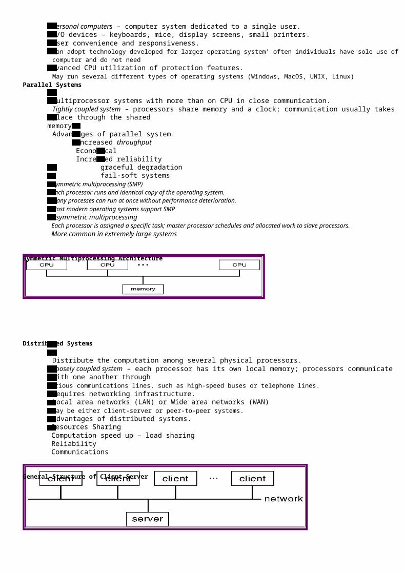
Symmetric multiprocessing (SMP) Each processor runs and identical copy of the operating system. Many processes can run at once without performance deterioration.
Most modern operating systems support SMP Asymmetric multiprocessing Each processor is assigned a specific task; master processor schedules and allocated work to slave processors.
More common in extremely large systems
Symmetric Multiprocessing Architecture
Distributed Systems
Distribute the computation among several physical processors. Loosely coupled system – each processor has its own local memory; processors communicate with one another through
various communications lines, such as high-speed buses or telephone lines. Requires networking infrastructure. Local area networks (LAN) or Wide area networks (WAN) May be either client-server or peer-to-peer systems. Advantages of distributed systems. Resources Sharing Computation speed up – load sharing Reliability Communications
General Structure of Client-Server
Clustered Systems
Clustering allows two or more systems to share storage. Provides high reliability. Asymmetric clustering: one server runs the application while other servers standby. Symmetric clustering: all N hosts are running the application.
Real-Time Systems
Often used as a control device in a dedicated application such as controlling scientific experiments, medical imaging systems, industrial control systems, and some display systems.
Well-defined fixed-time constraints. Real-Time systems may be either hard or soft real-time. Hard real-time:
Secondary storage limited or absent, data stored in short term memory, or read-only memory (ROM) Conflicts with time-sharing systems, not supported by general-purpose operating systems.
Soft real-time Limited utility in industrial control of robotics Useful in applications (multimedia, virtual reality) requiring advanced operating-system features.
Handheld Systems
Personal Digital Assistants (PDAs) Cellular telephones Issues:
Limited memory Slow processors Small display screens.
Computing Environments
Traditional computing Web-Based Computing Embedded Computing
Computer-System Architecture
Computer-System Operation
I/O devices and the CPU can execute concurrently. Each device controller is in charge of a particular device type. Each device controller has a local buffer. CPU moves data from/to main memory to/from local buffers I/O is from the device to local buffer of controller.

Device controller informs CPU that it has finished its operation by causing an interrupt.
Common Functions of Interrupts
Interrupt transfers control to the interrupt service routine generally, through the interrupt vector, which contains the addresses of all the service routines.
Interrupt architecture must save the address of the interrupted instruction. Incoming interrupts are disabled while another interrupt is being processed to prevent a lost interrupt. A trap is a software-generated interrupt caused either by an error or a user request. An operating system is interrupt driven.
Interrupt Handling
The operating system preserves the state of the CPU by storing registers and the program counter. Determines which type of interrupt has occurred: pollingvectored interrupt system Separate segments of code determine what action should be taken for each type of interrupt
I/O Structure
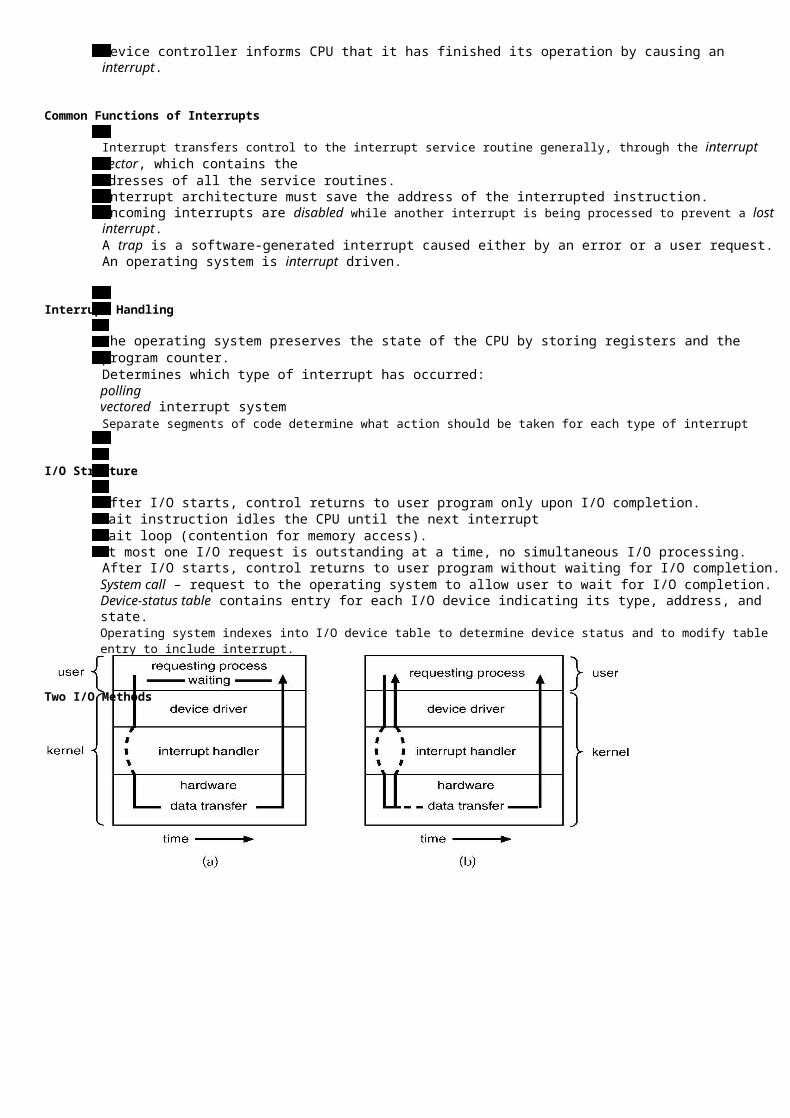
After I/O starts, control returns to user program only upon I/O completion. Wait instruction idles the CPU until the next interrupt Wait loop (contention for memory access). At most one I/O request is outstanding at a time, no simultaneous I/O processing. After I/O starts, control returns to user program without waiting for I/O completion. System call – request to the operating system to allow user to wait for I/O completion. Device-status table contains entry for each I/O device indicating its type, address, and state. Operating system indexes into I/O device table to determine device status and to modify table entry to include interrupt.
Two I/O Methods

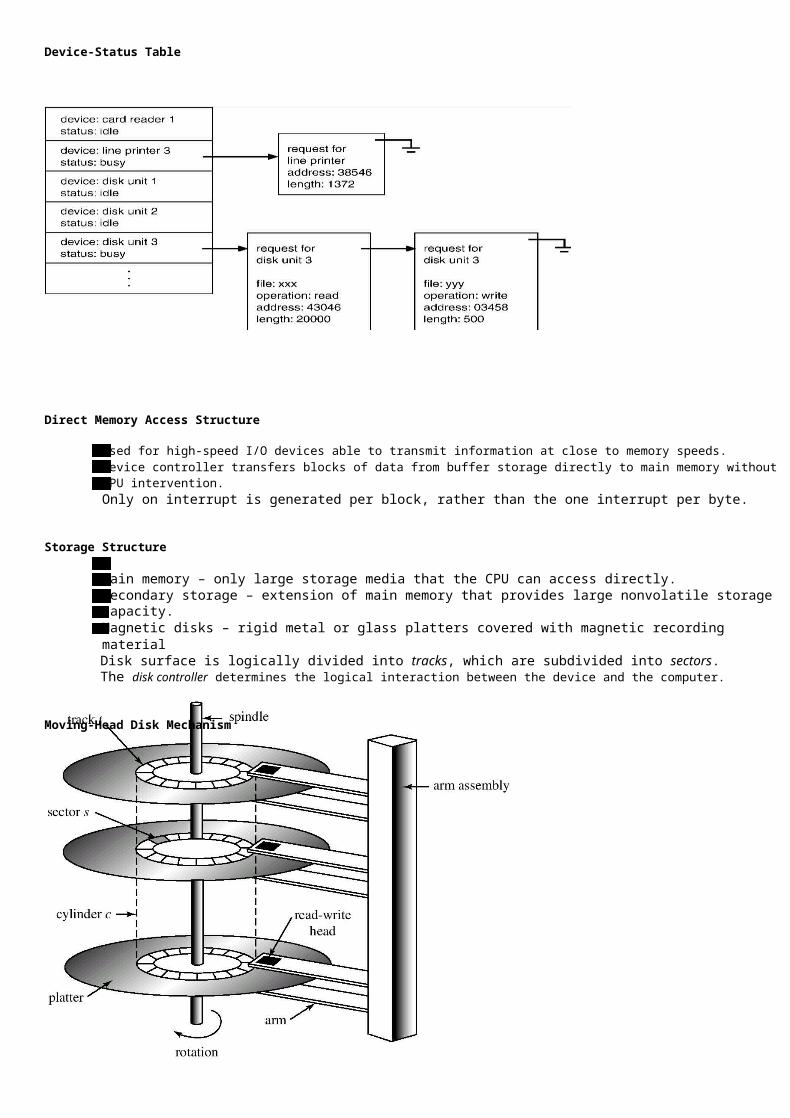
Device-Status Table
Direct Memory Access Structure
Used for high-speed I/O devices able to transmit information at close to memory speeds. Device controller transfers blocks of data from buffer storage directly to main memory without CPU intervention. Only on interrupt is generated per block, rather than the one interrupt per byte.
Storage Structure
Main memory – only large storage media that the CPU can access directly. Secondary storage – extension of main memory that provides large nonvolatile storage capacity. Magnetic disks – rigid metal or glass platters covered with magnetic recording material Disk surface is logically divided into tracks, which are subdivided into sectors. The disk controller determines the logical interaction between the device and the computer.
Moving-Head Disk Mechanism

Storage Hierarchy
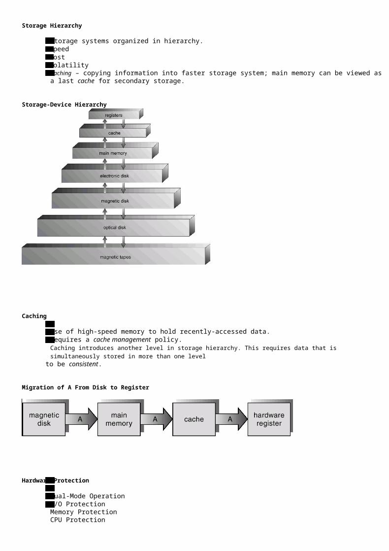
Storage systems organized in hierarchy. Speed Cost Volatility Caching – copying information into faster storage system; main memory can be viewed as a last cache for secondary storage.
Storage-Device Hierarchy
Caching
Use of high-speed memory to hold recently-accessed data. Requires a cache management policy. Caching introduces another level in storage hierarchy. This requires data that is simultaneously stored in more than one level
to be consistent.
Migration of A From Disk to Register
Hardware Protection
Dual-Mode Operation I/O Protection Memory Protection CPU Protection
Dual-Mode Operation
Sharing system resources requires operating system to ensure that an incorrect program cannot cause other programs to execute incorrectly.
Provide hardware support to differentiate between at least two modes of operations. 1.
2.
User mode – execution done on behalf of a user.
Monitor mode (also kernel mode or system mode) – execution done on behalf of operating system.
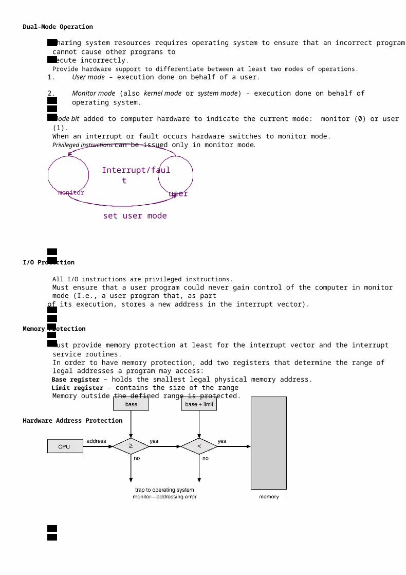
Mode bit added to computer hardware to indicate the current mode: monitor (0) or user (1). When an interrupt or fault occurs hardware switches to monitor mode. Privileged instructions can be issued only in monitor mode.
Interrupt/fault
monitor
I/O Protection
set user mode
user
All I/O instructions are privileged instructions. Must ensure that a user program could never gain control of the computer in monitor mode (I.e., a user program that, as part
of its execution, stores a new address in the interrupt vector).
Memory Protection
Must provide memory protection at least for the interrupt vector and the interrupt service routines. In order to have memory protection, add two registers that determine the range of legal addresses a program may access: Base register – holds the smallest legal physical memory address. Limit register – contains the size of the range Memory outside the defined range is protected.
Hardware Address Protection
Hardware Protection
When executing in monitor mode the operating system has unrestricted access to both monitor and user’s memory The load instructions for the base and limit registers are privileged instructions.
CPU Protection
Timer – interrupts computer after specified period to ensure operating system maintains control. Timer is decremented every clock tick. When timer reaches the value 0, an interrupt occurs. Timer commonly used to implement time sharing. Time also used to compute the current time. Load-timer is a privileged instruction.
Operating-System Structures
Common System Components
Process Management Main Memory Management File Management I/O System Management Secondary Management Networking Protection System Command-Interpreter System
Process Management
A process is a program in execution. A process needs certain resources, including CPU time, memory, files, and I/O devices, to accomplish its task.
The operating system is responsible for the following activities in connection with process management. Process creation and deletion. process suspension and resumption. Provision of mechanisms for: process synchronization process communication
Main-Memory Management
Memory is a large array of words or bytes, each with its own address. It is a repository of quickly accessible data shared by the CPU and I/O devices.
Main memory is a volatile storage device. It loses its contents in the case of system failure. The operating system is responsible for the following activities in connections with memory management: Keep track of which parts of memory are currently being used and by whom. Decide which processes to load when memory space becomes available. Allocate and deallocate memory space as needed.
File Management
A file is a collection of related information defined by its creator. Commonly, files represent programs (both source and object forms) and data.
The operating system is responsible for the following activities in connections with file management: File creation and deletion. Directory creation and deletion. Support of primitives for manipulating files and directories. Mapping files onto secondary storage. File backup on stable (nonvolatile) storage media.
I/O System Management
The I/O system consists of: A buffer-caching system A general device-driver interface Drivers for specific hardware devices
Secondary-Storage Management
Since main memory (primary storage) is volatile and too small to accommodate all data and programs permanently, the computer system must provide secondary storage to back up main memory.
Most modern computer systems use disks as the principle on-line storage medium, for both programs and data.
The operating system is responsible for the following activities in connection with disk management: Free space management Storage allocation Disk scheduling
Networking (Distributed Systems)
A distributed system is a collection processors that do not share memory or a clock. Each processor has its own localmemory.
The processors in the system are connected through a communication network. Communication takes place using a protocol. A distributed system provides user access to various system resources. Access to a shared resource allows: Computation speed-up Increased data availability Enhanced reliability
Protection System
Protection refers to a mechanism for controlling access by programs, processes, or users to both system and user resources. The protection mechanism must: distinguish between authorized and unauthorized usage. specify the controls to be imposed. provide a means of enforcement.
Command-Interpreter System
Many commands are given to the operating system by control statements which deal with: process creation and management I/O handling secondary-storage management main-memory management file-system access protection networking The program that reads and interprets control statements is called variously: command-line interpreter shell (in UNIX)
Its function is to get and execute the next command statement.
Operating System Services
Program execution – system capability to load a program into memory and to run it. I/O operations – since user programs cannot execute I/O operations directly, the operating system must provide some means
to perform I/O.
File-system manipulation – program capability to read, write, create, and delete files. Communications – exchange of information between processes executing either on the same computer or on different
systems tied together by a network. Implemented via shared memory or message passing. Error detection – ensure correct computing by detecting errors in the CPU and memory hardware, in I/O devices, or in user
programs.
Additional Operating System Functions
Additional functions exist not for helping the user, but rather for ensuring efficient system operations.
•Resource allocation – allocating resources to multiple users or multiple jobs running at the same time.
•Accounting – keep track of and record which users use how much and what kinds of computer resources for account billing orfor accumulating usage statistics. •Protection – ensuring that all access to system resources is controlled.
System Calls
System calls provide the interface between a running program and the operating system. Generally available as assembly-language instructions. Languages defined to replace assembly language for systems programming allow system calls to be made directly (e.g., C,
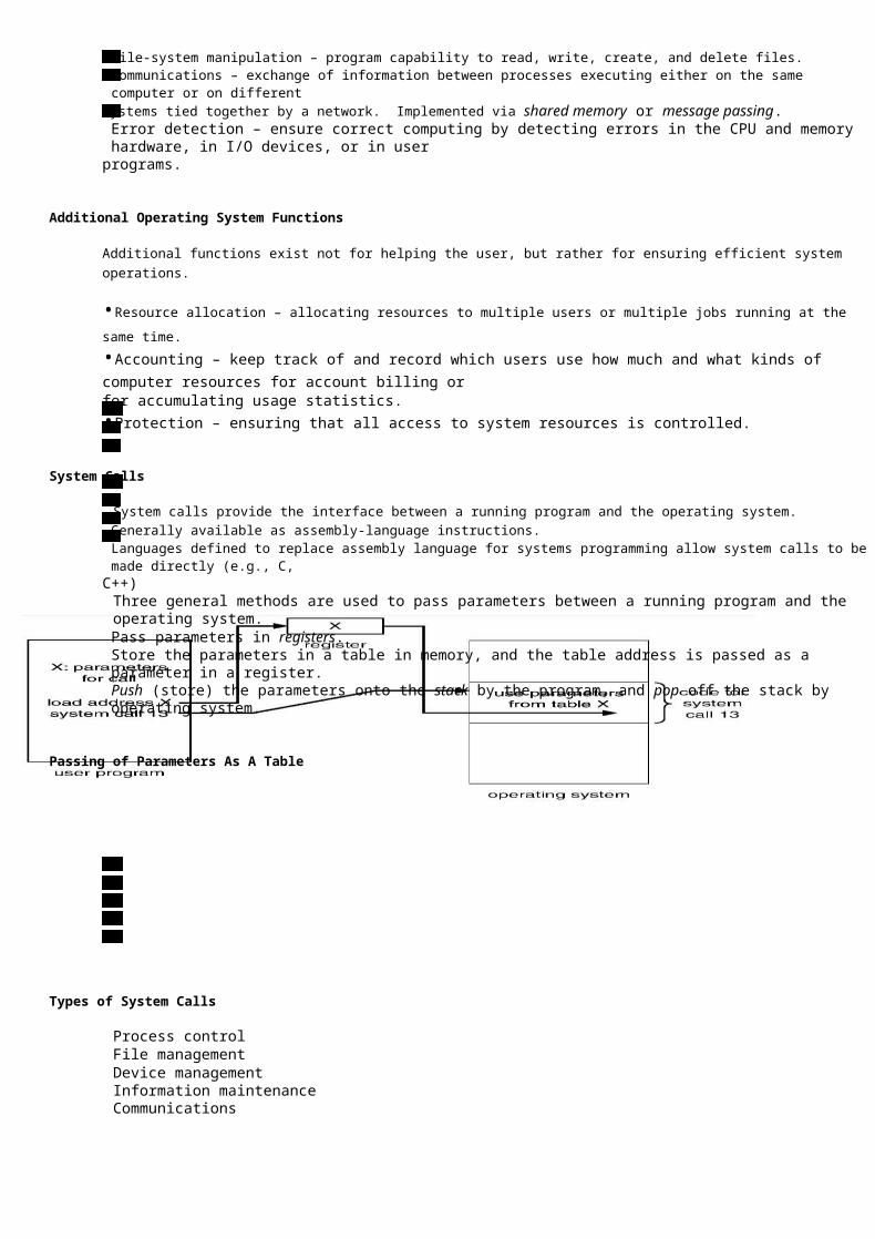
C++) Three general methods are used to pass parameters between a running program and the operating system. Pass parameters in registers. Store the parameters in a table in memory, and the table address is passed as a parameter in a register. Push (store) the parameters onto the stack by the program, and pop off the stack by operating system.
Passing of Parameters As A Table
Types of System Calls
Process control File management Device management Information maintenance Communications
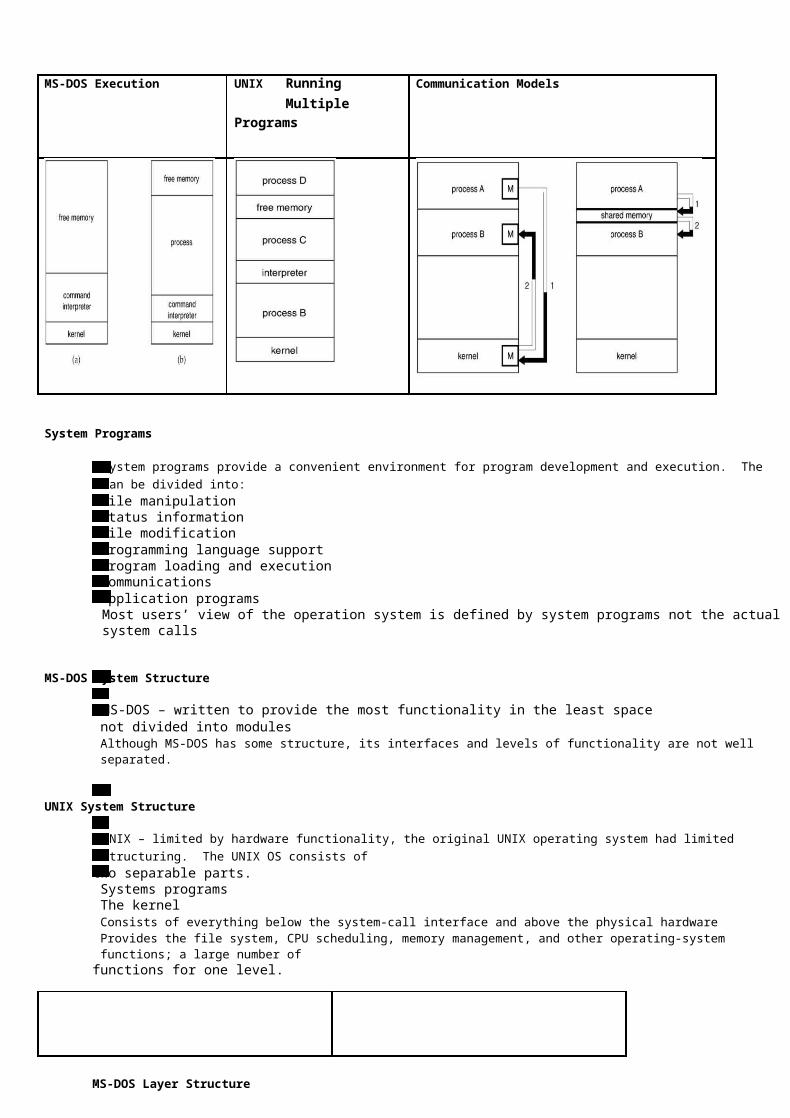
MS-DOS Execution
System Programs
UNIX Running Multiple
Programs
Communication Models
System programs provide a convenient environment for program development and execution. The can be divided into: File manipulation Status information File modification Programming language support Program loading and execution Communications Application programs Most users’ view of the operation system is defined by system programs not the actual system calls
MS-DOS System Structure
MS-DOS – written to provide the most functionality in the least space not divided into modules Although MS-DOS has some structure, its interfaces and levels of functionality are not well separated.
UNIX System Structure
UNIX – limited by hardware functionality, the original UNIX operating system had limited structuring. The UNIX OS consists of two separable parts.
Systems programs The kernel Consists of everything below the system-call interface and above the physical hardware Provides the file system, CPU scheduling, memory management, and other operating-system functions; a large number of
functions for one level.
MS-DOS Layer Structure
UNIX System Structure
Layered Approach
The operating system is divided into a number of layers (levels), each built on top of lower layers. The bottom layer (layer 0),is the hardware; the highest (layer N) is the user interface.
With modularity, layers are selected such that each uses functions (operations) and services of only lower-level layers.
An Operating System Layer
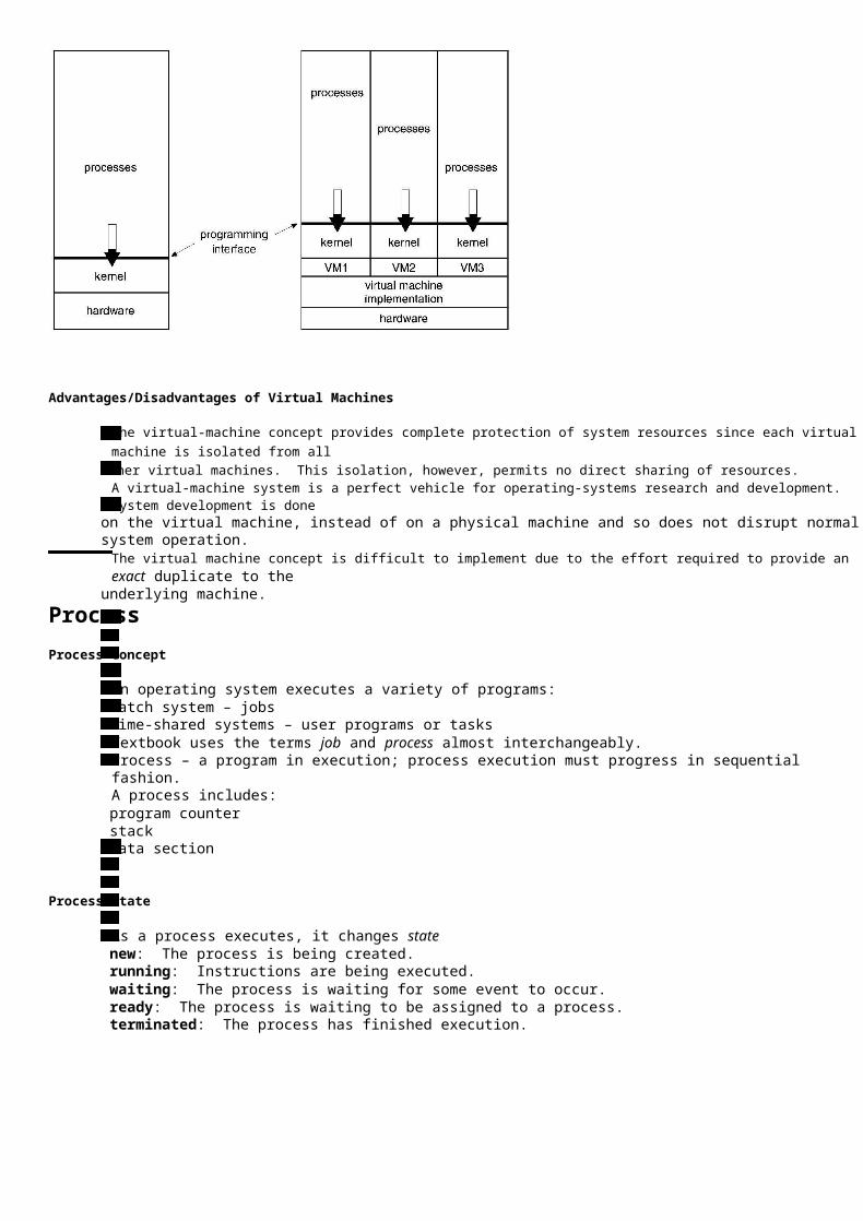
Virtual Machines
A virtual machine takes the layered approach to its logical conclusion. It treats hardware and the operating system kernel as though they were all hardware.
A virtual machine provides an interface identical to the underlying bare hardware. The operating system creates the illusion of multiple processes, each executing on its own processor with its own (virtual) memory. The resources of the physical computer are shared to create the virtual machines. CPU scheduling can create the appearance that users have their own processor. Spooling and a file system can provide virtual card readers and virtual line printers. A normal user time-sharing terminal serves as the virtual machine operator’s console
System Models
Advantages/Disadvantages of Virtual Machines
The virtual-machine concept provides complete protection of system resources since each virtual machine is isolated from allother virtual machines. This isolation, however, permits no direct sharing of resources.
A virtual-machine system is a perfect vehicle for operating-systems research and development. System development is done on the virtual machine, instead of on a physical machine and so does not disrupt normal system operation.
The virtual machine concept is difficult to implement due to the effort required to provide an exact duplicate to the underlying machine.
Process
Process Concept
An operating system executes a variety of programs: Batch system – jobs Time-shared systems – user programs or tasks Textbook uses the terms job and process almost interchangeably. Process – a program in execution; process execution must progress in sequential fashion. A process includes: program counter stack data section
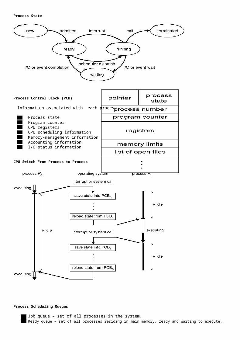
Process State
As a process executes, it changes statenew: The process is being created. running: Instructions are being executed. waiting: The process is waiting for some event to occur. ready: The process is waiting to be assigned to a process. terminated: The process has finished execution.

Process State
Process Control Block (PCB)
Information associated with each process.
Process state Program counter CPU registers CPU scheduling information Memory-management information Accounting information I/O status information
CPU Switch From Process to Process
Process Scheduling Queues
Job queue – set of all processes in the system. Ready queue – set of all processes residing in main memory, ready and waiting to execute.

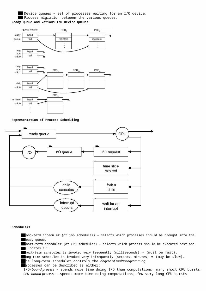
Device queues – set of processes waiting for an I/O device. Process migration between the various queues.
Ready Queue And Various I/O Device Queues
Representation of Process Scheduling
Schedulers
Long-term scheduler (or job scheduler) – selects which processes should be brought into the ready queue. Short-term scheduler (or CPU scheduler) – selects which process should be executed next and allocates CPU. Short-term scheduler is invoked very frequently (milliseconds) (must be fast). Long-term scheduler is invoked very infrequently (seconds, minutes) (may be slow). The long-term scheduler controls the degree of multiprogramming. Processes can be described as either: I/O-bound process – spends more time doing I/O than computations, many short CPU bursts. CPU-bound process – spends more time doing computations; few very long CPU bursts.
Context Switch
When CPU switches to another process, the system must save the state of the old process and load the saved state for the new process. Context-switch time is overhead; the system does no useful work while switching. Time dependent on hardware support.
Process Creation
Parent process create children processes, which, in turn create other processes, forming a tree of processes. Resource sharing Parent and children share all resources. Children share subset of parent’s resources Parent and child share no resources. Execution Parent and children execute concurrently. Parent waits until children terminate. Address space Child duplicate of parent. Child has a program loaded into it. UNIX examples fork system call creates new process exec system call used after a fork to replace the process’ memory space with a new program
Process Termination
Process executes last statement and asks the operating system to decide it (exit). Output data from child to parent (via wait). Process’ resources are deallocated by operating system Parent may terminate execution of children processes (abort). Child has exceeded allocated resources. Task assigned to child is no longer required. Parent is exiting. Operating system does not allow child to continue if its parent terminates. Cascading termination.
Cooperating Processes
Independent process cannot affect or be affected by the execution of another process. Cooperating process can affect or be affected by the execution of another process Advantages of process cooperation Information sharing Computation speed-up Modularity Convenience
Producer-Consumer Problem
Paradigm for cooperating processes, producer process produces information that is consumed by a consumer process. unbounded-buffer places no practical limit on the size of the buffer. bounded-buffer assumes that there is a fixed buffer size.
Bounded-Buffer – Shared-Memory Solution
Shared data #define BUFFER_SIZE 10
Typedef struct {
. . .
} item;
item buffer[BUFFER_SIZE];
int in = 0;
int out = 0;
Solution is correct, but can only use BUFFER_SIZE-1 elements
Bounded-Buffer – Producer Process
Item nextProduced;
while (1) {
while (((in + 1) % BUFFER_SIZE) == out)
; /* do nothing */
buffer[in] = nextProduced;
in = (in + 1) % BUFFER_SIZE;
}
Bounded-Buffer – Consumer Process
item nextConsumed;
while (1) {
while (in == out)
; /* do nothing */
nextConsumed = buffer[out];
out = (out + 1) % BUFFER_SIZE;
}
Interprocess Communication (IPC)
Mechanism for processes to communicate and to synchronize their actions. Message system – processes communicate with each other without resorting
to shared variables.
IPC facility provides two operations: send(message) – message size fixed or variable receive(message) If P and Q wish to communicate, they need to:

establish a communication link between them exchange messages via send/receive Implementation of communication link physical (e.g., shared memory, hardware bus) logical (e.g., logical properties)
Direct Communication
Processes must name each other explicitly: send (P, message) – send a message to process P receive(Q, message) – receive a message from process Q Properties of communication link Links are established automatically. A link is associated with exactly one pair of communicating processes. Between each pair there exists exactly one link. The link may be unidirectional, but is usually bi-directional.
Indirect Communication
Messages are directed and received from mailboxes (also referred to as ports). Each mailbox has a unique id. Processes can communicate only if they share a mailbox. Properties of communication link Link established only if processes share a common mailbox A link may be associated with many processes. Each pair of processes may share several communication links. Link may be unidirectional or bi-directional.
Operations create a new mailbox send and receive messages through mailbox destroy a mailbox Primitives are defined as:
send(A, message) – send a message to mailbox A
receive(A, message) – receive a message from mailbox A
Mailbox sharing P1, P2, and P3 share mailbox A. P1, sends; P2 and P3 receive. Who gets the message?
Solutions Allow a link to be associated with at most two processes. Allow only one process at a time to execute a receive operation. Allow the system to select arbitrarily the receiver. Sender is notified who the receiver was.
Synchronization
Message passing may be either blocking or non-blocking. Blocking is considered synchronous Non-blocking is considered asynchronous send and receive primitives may be either blocking or non-blocking.
Buffering
Queue of messages attached to the link; implemented in one of three ways. 1.
2.
Zero capacity – 0 messages Sender must wait for receiver (rendezvous).
Bounded capacity – finite length of n messages Sender must wait if link full.

3. Unbounded capacity – infinite length Sender never waits.
Client-Server Communication
Sockets , Remote Procedure Calls, Remote Method Invocation (Java)
Sockets
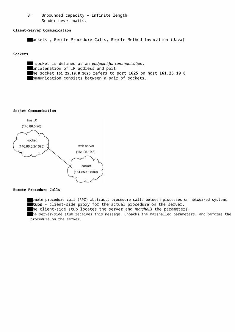
A socket is defined as an endpoint for communication. Concatenation of IP address and port The socket 161.25.19.8:1625 refers to port 1625 on host 161.25.19.8 Communication consists between a pair of sockets.
Socket Communication
Remote Procedure Calls
Remote procedure call (RPC) abstracts procedure calls between processes on networked systems. Stubs – client-side proxy for the actual procedure on the server. The client-side stub locates the server and marshalls the parameters. The server-side stub receives this message, unpacks the marshalled parameters, and peforms the procedure on the server.
Execution of RPC
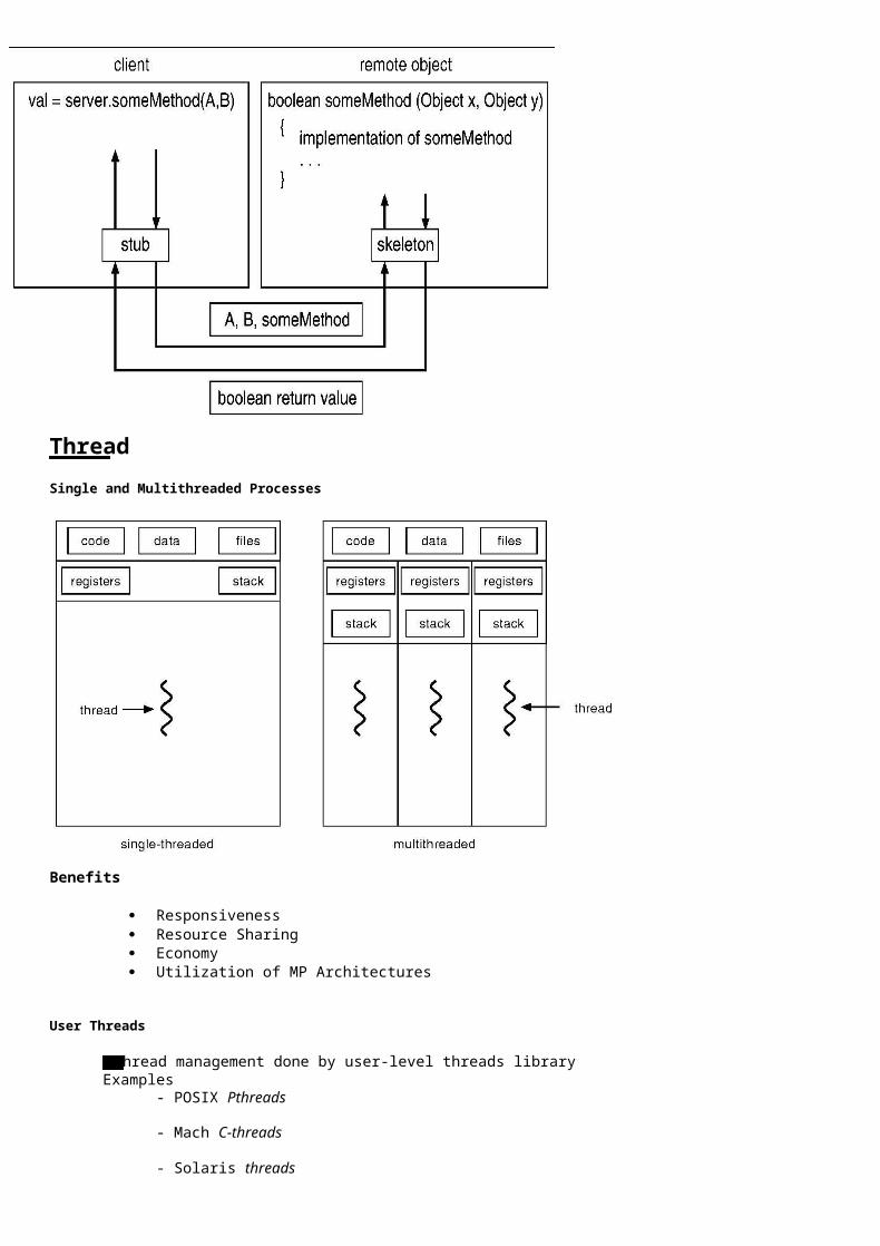
Remote Method Invocation
Remote Method Invocation (RMI) is a Java mechanism similar to RPCs. RMI allows a Java program on one machine to invoke a method on a remote object.
Marshalling Parameters
Thread
Single and Multithreaded Processes
Benefits
Responsiveness Resource Sharing Economy Utilization of MP Architectures
User Threads
Thread management done by user-level threads library Examples
- POSIX Pthreads
- Mach C-threads
- Solaris threads
Kernel Threads
Supported by the Kernel Examples
- Windows 95/98/NT/2000
- Solaris
- Tru64 UNIX
- BeOS
- Linux
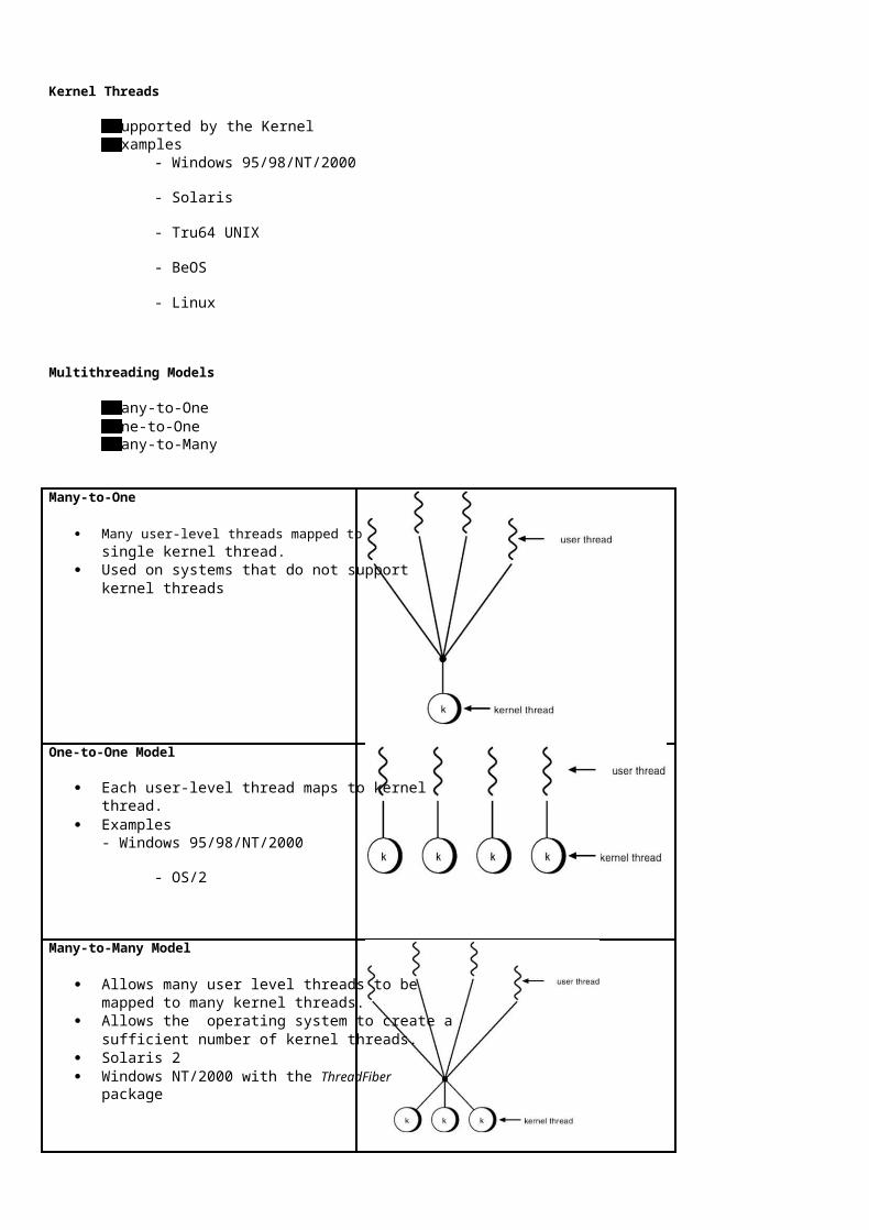
Multithreading Models
Many-to-One One-to-One Many-to-Many
Many-to-One
Many user-level threads mapped to single kernel thread.
Used on systems that do not supportkernel threads
One-to-One Model
Each user-level thread maps to kernelthread.
Examples - Windows 95/98/NT/2000
- OS/2
Many-to-Many Model
Allows many user level threads to be mapped to many kernel threads.
Allows the operating system to create a sufficient number of kernel threads.
Solaris 2 Windows NT/2000 with the ThreadFiber
package

Threading Issues
Semantics of fork() and exec() system calls. Thread cancellation. Signal handling Thread pools Thread specific data
Pthreads
a POSIX standard (IEEE 1003.1c) API for thread creation and synchronization. API specifies behavior of the thread library, implementation is up to development of the library. Common in UNIX operating systems.
Windows 2000 Threads
Implements the one-to-one mapping. Each thread contains
- a thread id
- register set
- separate user and kernel stacks
- private data storage area
Linux Threads
Linux refers to them as tasks rather than threads. Thread creation is done through clone() system call. Clone() allows a child task to share the address space of the parent task (process)
Java Threads
Java threads may be created by: Extending Thread class Implementing the Runnable interface
Java threads are managed by the JVM.

PART – A (2 MARKS)
1. What is an operating system?
UNIT I - PROCESSES AND THREADS
2. Differentiate between tightly coupled systems and loosely coupled systems.
3. What is the kernel?
4. What are batch systems?
5. What are privileged instructions?
6. What do you mean by system calls?
7. What is a process?
8. What is process control block?
9. What are schedulers?
10. What are the use of job queues, ready queues and device queues?
11. What is meant by context switch?
12. What is independent process?
13. What is co-operative process?
14. What are the benefits OS co-operating processes?
15. How can a user program disturb the normal operation of the system?
16. State the advantage of multiprocessor system?
17. What is the use of inter process communication.
18. What is a thread?
19. What are the benefits of multithreaded programming?
20. Compare user threads and kernel threads.
21. What is the use of fork and exec system calls?
22. Define thread cancellation & target thread.
23. What are the different ways in which a thread can be cancelled?
24. What is a process state and mention the various states of a process?
PART B
1. Write about the various system calls. (16)
2. Discuss briefly the various issues involved in implementing Inter Process Communication (16)

3. Explain in detail about an overview of threads. (16)
4. Explain in detail about the threading issues and types of treads (16)
5. Discuss the process Concept, process Scheduling and Cooperating Processes (16)

UNIT II PROCESS SCHEDULING AND SYNCHRONIZATION
CPU scheduling – Scheduling criteria – Scheduling algorithms – Multiple – Processor scheduling – Real time scheduling – Algorithm evaluation – Case study – Process scheduling in Linux – Process synchronization – The critical-section problem – Synchronization hardware – Semaphores – Classic problems of synchronization –Critical regions – Monitors – Deadlock – System model – Deadlock characterization – Methods for handling deadlocks – Deadlockprevention – Deadlock avoidance – Deadlock detection – Recovery from deadlock.
UNIT-2
CPU Scheduling
1. Basic Concepts 2. Scheduling Criteria 3. Scheduling Algorithms 4. Multiple-Processor Scheduling 5. Real-Time Scheduling 6. Algorithm Evaluation
Basic Concepts
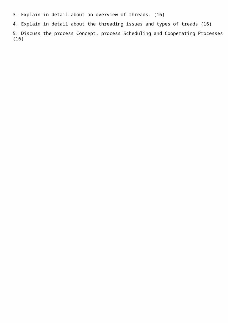
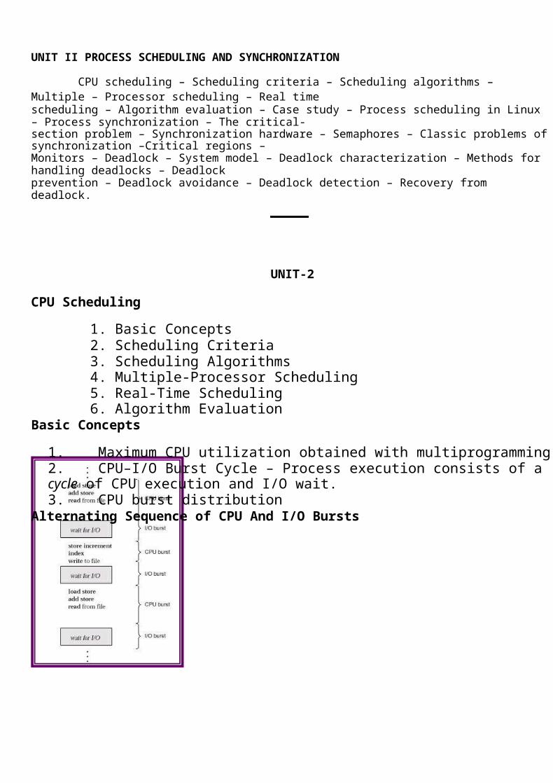
1. Maximum CPU utilization obtained with multiprogramming 2. CPU–I/O Burst Cycle – Process execution consists of a cycle of CPU execution and I/O wait. 3. CPU burst distribution
Alternating Sequence of CPU And I/O Bursts
Histogram of CPU-burst Times
CPU Scheduler
Selects from among the processes in memory that are ready to execute, and allocates
the CPU to one of them. CPU scheduling decisions may take place when a process:
1.
2.
3.
4.
Switches from running to waiting state.
Switches from running to ready state.
Switches from waiting to ready.
Terminates.
Scheduling under 1 and 4 is nonpreemptive. All other scheduling is preemptive.
Dispatcher
1. Dispatcher module gives control of the CPU to the process selected by the short-termscheduler; this involves:
a. switching context b. switching to user mode c. jumping to the proper location in the user program to restart that program
2. Dispatch latency – time it takes for the dispatcher to stop one process and start another
running. Scheduling Criteria
1. CPU utilization – keep the CPU as busy as possible 2. Throughput – # of processes that complete their execution per time unit 3. Turnaround time – amount of time to execute a particular process 4. Waiting time – amount of time a process has been waiting in the ready queue 5. Response time – amount of time it takes from when a request was submitted until the first

response is produced, not output (for time-sharing environment)
Optimization Criteria
1. Max CPU utilization 2. Max throughput 3. Min turnaround time 4. Min waiting time 5. Min response time
Scheduling Algorithm
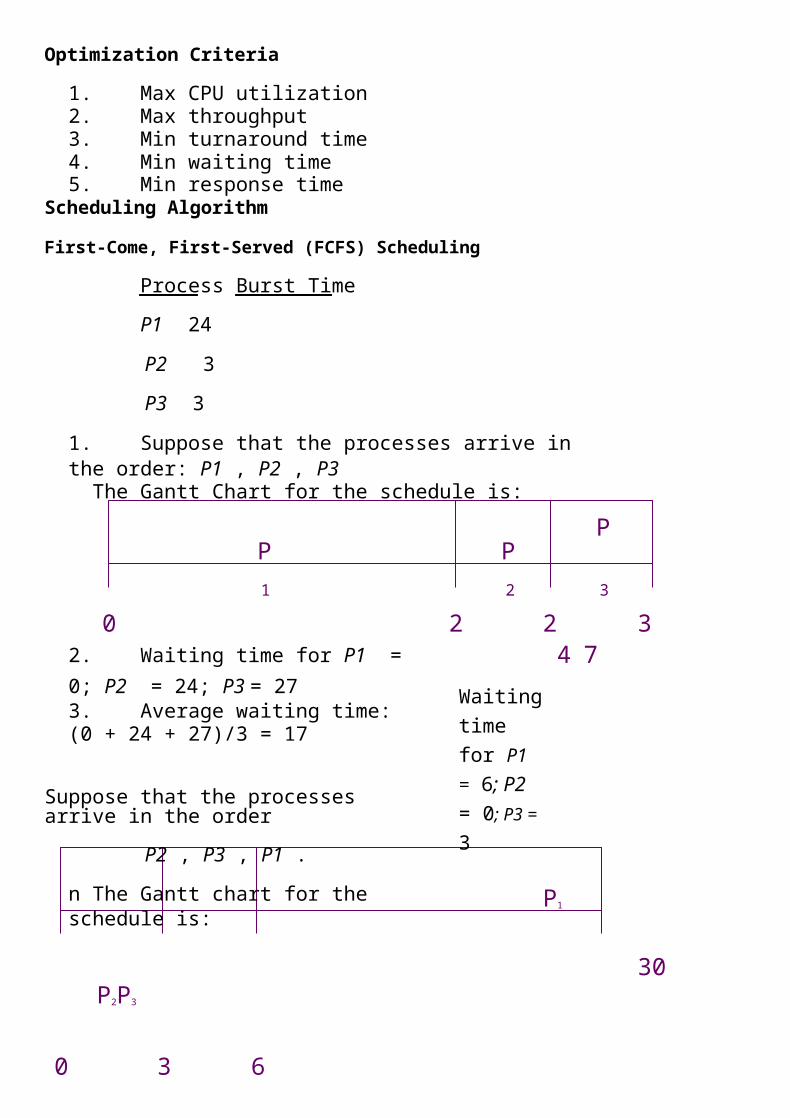
First-Come, First-Served (FCFS) Scheduling
Process
P1 24
P2 3
P3 3
Burst Time
1. Suppose that the processes arrive in the order: P1 , P2 , P3 The Gantt Chart for the schedule is:
P P P
0
1
2
2
2
3
32. Waiting time for P1 = 0; P2 = 24; P3 = 27 3. Average waiting time: (0 + 24 + 27)/3 = 17
Suppose that the processes arrive in the order
P2 , P3 , P1 .
n The Gantt chart for the schedule is:
P2P3
0 3 6
Waiting time for P1 = 6; P2 = 0; P3 = 3
4
P1
7
30
0
Average waiting time: (6 + 0 + 3)/3 = 3
Much better than previous case.
Convoy effect short process behind long process
Shortest-Job-First (SJR) Scheduling
1. Associate with each process the length of its next CPU burst. Use these lengths toschedule the process with the shortest time.
2. Two schemes: a. nonpreemptive – once CPU given to the process it cannot be preempted until
completes its CPU burst. b. preemptive – if a new process arrives with CPU burst length less than remaining
time of current executing process, preempt. This scheme is know as the Shortest-Remaining-Time-First (SRTF).
3. SJF is optimal – gives minimum average waiting time for a given set of processes.
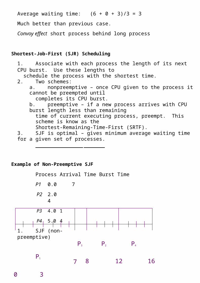
Example of Non-Preemptive SJF
Process Arrival Time Burst Time
P1 0.0 7
P2 2.0 4
P3 4.0 1
P4 5.0 4
1. SJF (non-preemptive)
P1
0 3
P3
7 8
P2
12
P4
16
Average waiting time = (0 + 6 + 3 + 7)/4 - 4
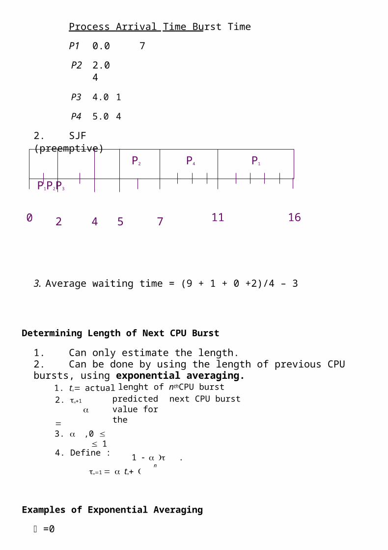
Example of Preemptive SJF

Process Arrival Time Burst Time
P1 0.0 7
P2 2.0 4
P3 4.0 1
P4 5.0 4
2. SJF (preemptive)
P1P2P3 P2 P4 P1
0 2 4 5 7 11 16
3. Average waiting time = (9 + 1 + 0 +2)/4 – 3
Determining Length of Next CPU Burst
1. Can only estimate the length. 2. Can be done by using the length of previous CPU bursts, using exponential averaging.
1. tnactual lenght of nthCPU burst
2. n1
predicted value for the
next CPU burst
3. ,0 14. Define :
1 .
n1 tnn
Examples of Exponential Averaging
=0
n+1 = n
Recent history does not count.

=1
n+1 = tn
Only the actual last CPU burst counts.
If we expand the formula, we get:
n+1 = tn+(1 - ) tn -1 +
+(1 - )j tn -1 +
+(1 - )n=1 tn 0
Since both and (1 - ) are less than or equal to 1, each successive term has less weight than its predecessor.
Priority Scheduling
1. A priority number (integer) is associated with each process 2. The CPU is allocated to the process with the highest priority (smallest integer highest
priority). a. Preemptive b. nonpreemptive
3. SJF is a priority scheduling where priority is the predicted next CPU burst time. 4. Problem Starvation – low priority processes may never execute. 5. Solution Aging – as time progresses increase the priority of the process.
Round Robin (RR)
1. Each process gets a small unit of CPU time (time quantum), usually 10-100 milliseconds.
After this time has elapsed, the process is preempted and added to the end of the readyqueue.
2. If there are n processes in the ready queue and the time quantum is q, then each process
gets 1/n of the CPU time in chunks of at most q time units at once. No process waits morethan (n-1)q time units.
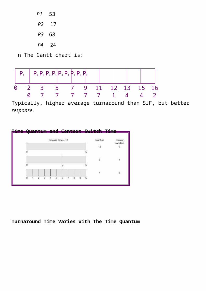
3. Performance a. q large FIFO
b. q small q must be large with respect to context switch, otherwise overhead is too
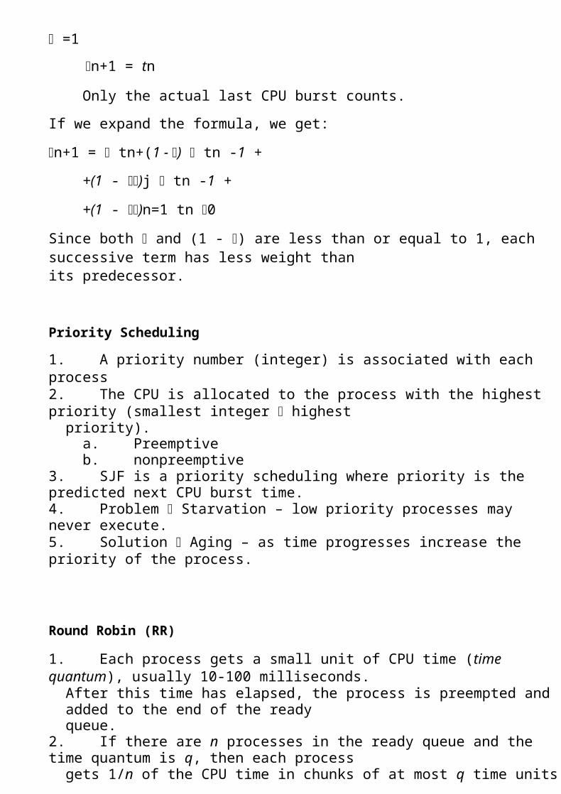
high. Example of RR with Time Quantum = 20
Process Burst Time
P1 53
P2 17
P3 68
P4 24
n The Gantt chart is:
0
P1
2
P2 P3 P4 P1 P3 P4 P1 P3 P3
3 5 7 9 11 12 13 15 160 7 7 7 7 7 1 4 4 2
Typically, higher average turnaround than SJF, but better response.
Time Quantum and Context Switch Time
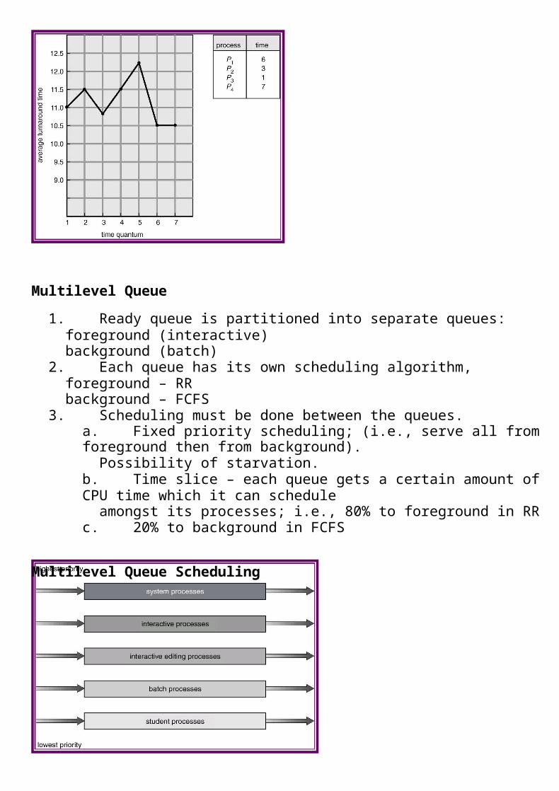
Turnaround Time Varies With The Time Quantum

Multilevel Queue
1. Ready queue is partitioned into separate queues: foreground (interactive) background (batch)
2. Each queue has its own scheduling algorithm, foreground – RR background – FCFS
3. Scheduling must be done between the queues. a. Fixed priority scheduling; (i.e., serve all from foreground then from background).
Possibility of starvation. b. Time slice – each queue gets a certain amount of CPU time which it can schedule
amongst its processes; i.e., 80% to foreground in RR c. 20% to background in FCFS
Multilevel Queue Scheduling
Multilevel Feedback Queue
1. A process can move between the various queues; aging can be implemented this way. 2. Multilevel-feedback-queue scheduler defined by the following parameters:
a. number of queues b. scheduling algorithms for each queue c. method used to determine when to upgrade a process d. method used to determine when to demote a process e. method used to determine which queue a process will enter when that process
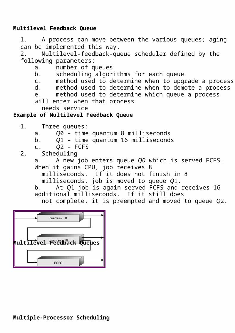
needs service Example of Multilevel Feedback Queue
1. Three queues: a. Q0 – time quantum 8 milliseconds b. Q1 – time quantum 16 milliseconds c. Q2 – FCFS
2. Scheduling a. A new job enters queue Q0 which is served FCFS. When it gains CPU, job receives 8
milliseconds. If it does not finish in 8 milliseconds, job is moved to queue Q1. b. At Q1 job is again served FCFS and receives 16 additional milliseconds. If it still does
not complete, it is preempted and moved to queue Q2.
Multilevel Feedback Queues
Multiple-Processor Scheduling
1. CPU scheduling more complex when multiple CPUs are available. 2. Homogeneous processors within a multiprocessor. 3. Load sharing
4. Asymmetric multiprocessing – only one processor accesses the system data structures,
alleviating the need for data sharing.
Real-Time Scheduling
1. Hard real-time systems – required to complete a critical task within a guaranteed amount
of time. 2. Soft real-time computing – requires that critical processes receive priority over less
fortunate ones.
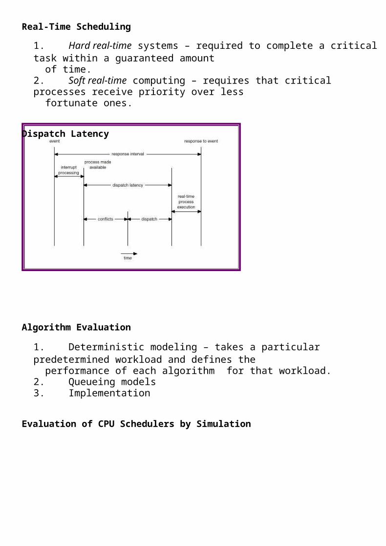
Dispatch Latency
Algorithm Evaluation
1. Deterministic modeling – takes a particular predetermined workload and defines the performance of each algorithm for that workload.
2. Queueing models 3. Implementation
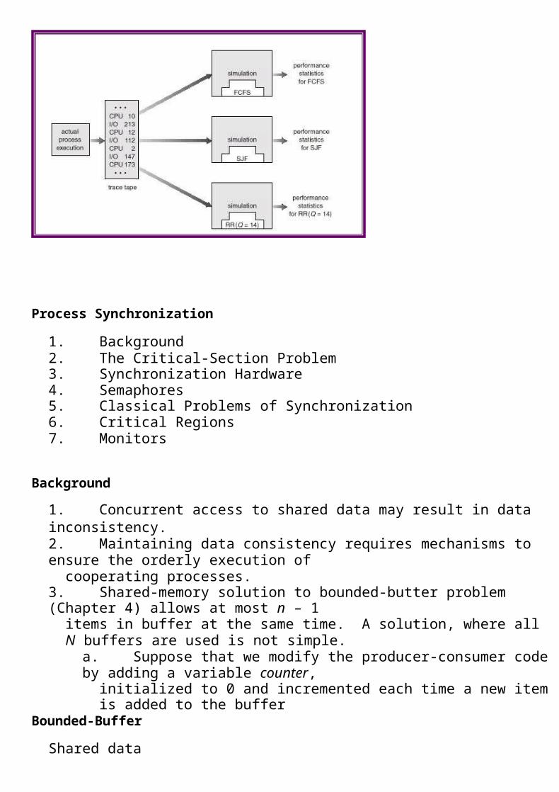
Evaluation of CPU Schedulers by Simulation

Process Synchronization
1. Background 2. The Critical-Section Problem 3. Synchronization Hardware 4. Semaphores 5. Classical Problems of Synchronization 6. Critical Regions 7. Monitors
Background
1. Concurrent access to shared data may result in data inconsistency. 2. Maintaining data consistency requires mechanisms to ensure the orderly execution of
cooperating processes. 3. Shared-memory solution to bounded-butter problem (Chapter 4) allows at most n – 1
items in buffer at the same time. A solution, where all N buffers are used is not simple.
a. Suppose that we modify the producer-consumer code by adding a variable counter,
initialized to 0 and incremented each time a new item is added to the buffer Bounded-Buffer
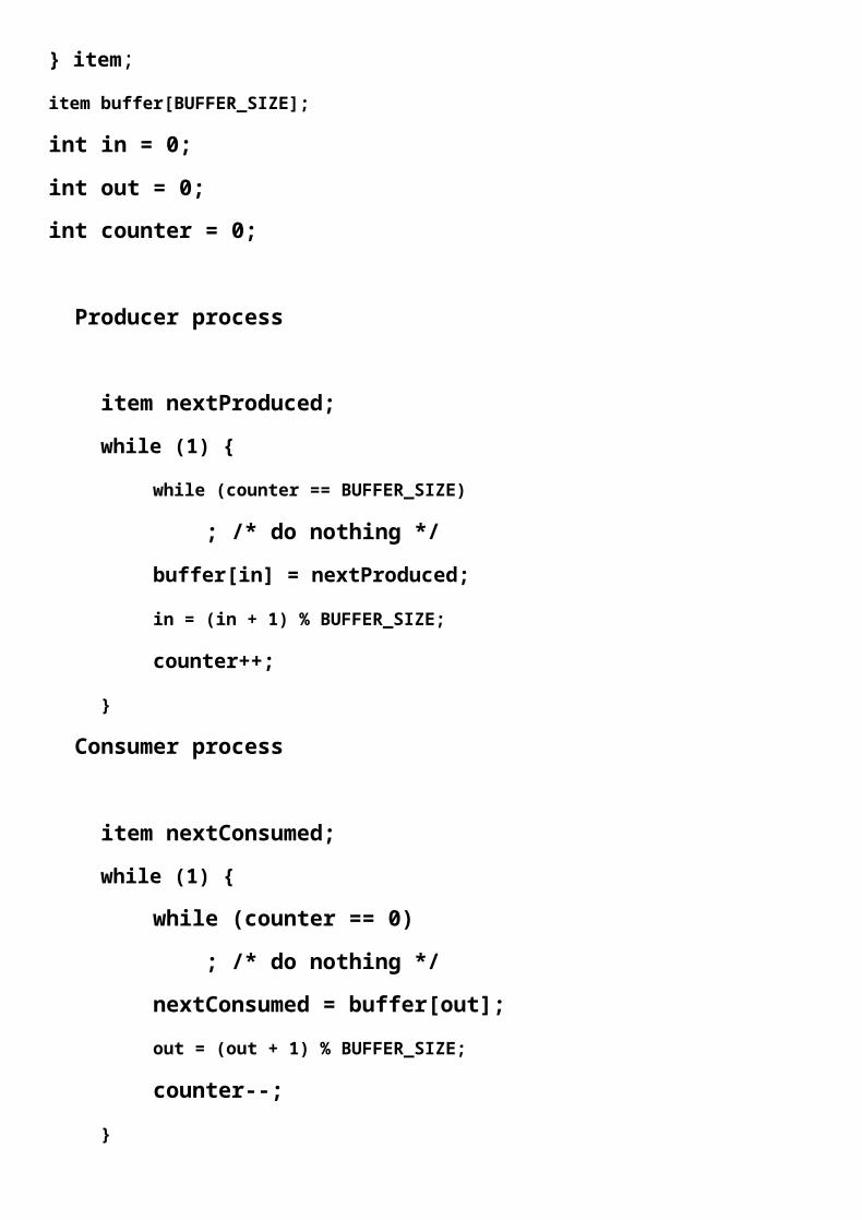
Shared data
#define BUFFER_SIZE 10
typedef struct {
. . .

} item;
item buffer[BUFFER_SIZE];
int in = 0;
int out = 0;
int counter = 0;
Producer process
item nextProduced;
while (1) {
while (counter == BUFFER_SIZE)
; /* do nothing */
buffer[in] = nextProduced;
in = (in + 1) % BUFFER_SIZE;
counter++;
}
Consumer process
item nextConsumed;
while (1) {
while (counter == 0)
; /* do nothing */
nextConsumed = buffer[out];
out = (out + 1) % BUFFER_SIZE;
counter--;
}
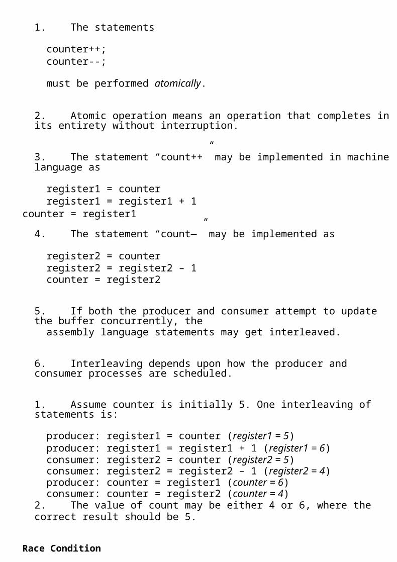
1. The statements
counter++; counter--;
must be performed atomically.
2. Atomic operation means an operation that completes in its entirety without interruption.
3. The statement “count++” may be implemented in machine language as
register1 = counter register1 = register1 + 1
counter = register1
4. The statement “count—” may be implemented as
register2 = counter register2 = register2 – 1 counter = register2
5. If both the producer and consumer attempt to update the buffer concurrently, the assembly language statements may get interleaved.
6. Interleaving depends upon how the producer and consumer processes are scheduled.
1. Assume counter is initially 5. One interleaving of statements is:
producer: register1 = counter (register1 = 5) producer: register1 = register1 + 1 (register1 = 6) consumer: register2 = counter (register2 = 5) consumer: register2 = register2 – 1 (register2 = 4) producer: counter = register1 (counter = 6) consumer: counter = register2 (counter = 4)
2. The value of count may be either 4 or 6, where the correct result should be 5.
Race Condition
1. Race condition: The situation where several processes access – and manipulate shared
data concurrently. The final value of the shared data depends upon which process finisheslast.
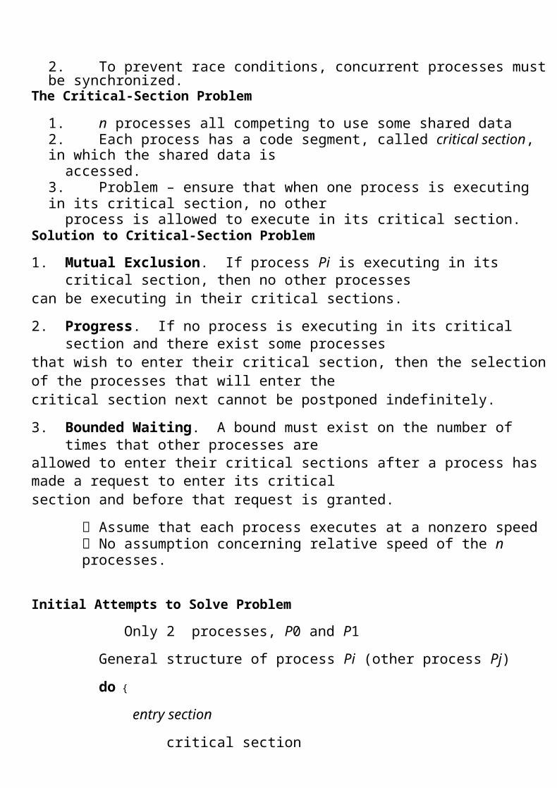
2. To prevent race conditions, concurrent processes must be synchronized. The Critical-Section Problem
1. n processes all competing to use some shared data 2. Each process has a code segment, called critical section, in which the shared data is
accessed. 3. Problem – ensure that when one process is executing in its critical section, no other
process is allowed to execute in its critical section. Solution to Critical-Section Problem
1. Mutual Exclusion. If process Pi is executing in its critical section, then no other processes
can be executing in their critical sections.
2. Progress. If no process is executing in its critical section and there exist some processes
that wish to enter their critical section, then the selection of the processes that will enter thecritical section next cannot be postponed indefinitely.
3. Bounded Waiting. A bound must exist on the number of times that other processes are
allowed to enter their critical sections after a process has made a request to enter its criticalsection and before that request is granted.
Assume that each process executes at a nonzero speed No assumption concerning relative speed of the n processes.
Initial Attempts to Solve Problem
Only 2 processes, P0 and P1
General structure of process Pi (other process Pj)
do {
entry section
critical section
exit section
reminder section
} while (1);

Processes may share some common variables to synchronize their actions.
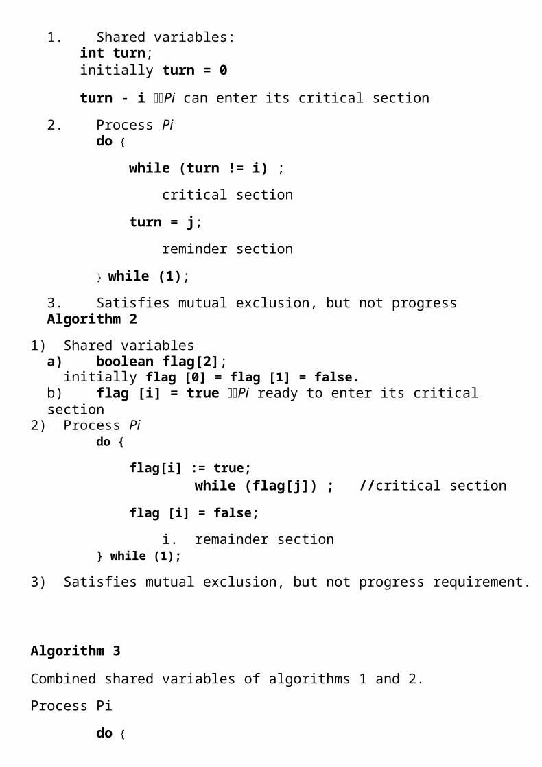
Algorithm 1
1. Shared variables: int turn; initially turn = 0
turn - i Pi can enter its critical section
2. Process Pido {
while (turn != i) ;
critical section
turn = j;
reminder section
} while (1);
3. Satisfies mutual exclusion, but not progress Algorithm 2
1) Shared variables a) boolean flag[2];
initially flag [0] = flag [1] = false. b) flag [i] = true Pi ready to enter its critical section
2) Process Pido {
flag[i] := true;
while (flag[j]) ; //critical section
flag [i] = false;
i. remainder section } while (1);
3) Satisfies mutual exclusion, but not progress requirement.
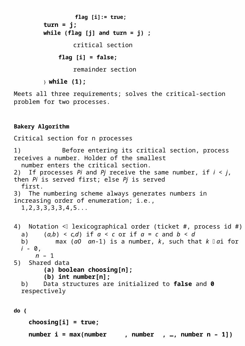
Algorithm 3
Combined shared variables of algorithms 1 and 2.
Process Pi
do {
flag [i]:= true;
turn = j; while (flag [j] and turn = j) ;
critical section
flag [i] = false;
remainder section
} while (1);
Meets all three requirements; solves the critical-section problem for two processes.
Bakery Algorithm
Critical section for n processes
1) Before entering its critical section, process receives a number. Holder of the smallest
number enters the critical section. 2) If processes Pi and Pj receive the same number, if i < j, then Pi is served first; else Pj is served
first. 3) The numbering scheme always generates numbers in increasing order of enumeration; i.e.,
1,2,3,3,3,3,4,5...
4) Notation < lexicographical order (ticket #, process id #) a) (a,b) < c,d) if a < c or if a = c and b < db) max (a0 an-1) is a number, k, such that k ai for i - 0,
n – 1 5) Shared data
(a) boolean choosing[n]; (b) int number[n];
b) Data structures are initialized to false and 0 respectively
do {
choosing[i] = true;
number i = max(number , number , …, number n – 1])+1;
choosing[i] = false;
for (j = 0; j < n; j++) {
while (choosing[j]) ;
}
while ((number[j] != 0) && (number[j,j] < number[i,i])) ;
critical section
number[i] = 0;
remainder section
} while (1);
Synchronization Hardware
Test and modify the content of a word atomically .
boolean TestAndSet(boolean &target) {
boolean rv = target;
tqrget = true;
return rv;
}
Mutual Exclusion with Test-and-Set
Shared data: boolean lock = false;
Process Pi
do {
while (TestAndSet(lock)) ;
critical section
lock = false;
remainder section
}
Synchronization Hardware
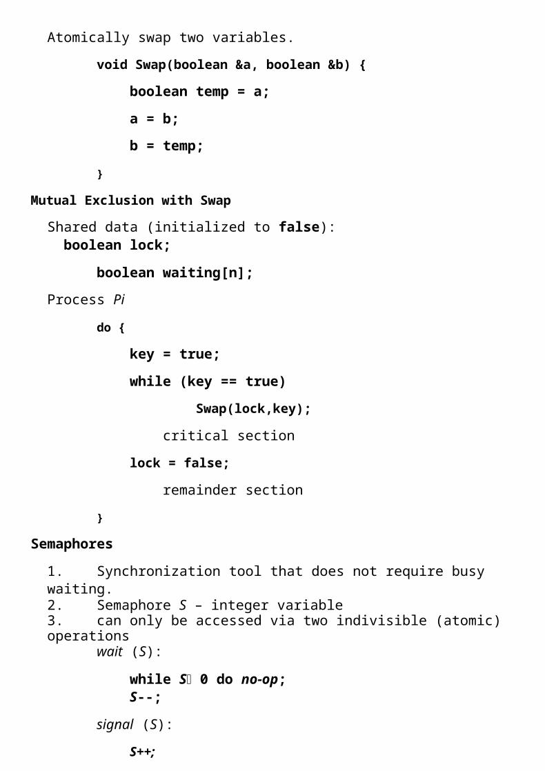
Atomically swap two variables.
void Swap(boolean &a, boolean &b) {
boolean temp = a;
a = b;
b = temp;
}
Mutual Exclusion with Swap
Shared data (initialized to false): boolean lock;
boolean waiting[n];
Process Pi
do {
key = true;
while (key == true)
Swap(lock,key);
critical section
lock = false;
remainder section
}
Semaphores
1. Synchronization tool that does not require busy waiting. 2. Semaphore S – integer variable 3. can only be accessed via two indivisible (atomic) operations
wait (S):
while S 0 do no-op; S--;
signal (S):
S++;
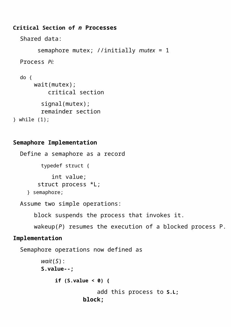
Critical Section of n Processes
Shared data:
semaphore mutex; //initially mutex = 1
Process Pi:
do { wait(mutex); critical section
signal(mutex); remainder section } while (1);
Semaphore Implementation
Define a semaphore as a record
typedef struct {
int value; struct process *L; } semaphore;
Assume two simple operations:
block suspends the process that invokes it.
wakeup(P) resumes the execution of a blocked process P.
Implementation
Semaphore operations now defined as
wait(S): S.value--;
if (S.value < 0) {
add this process to S.L;
block;

}
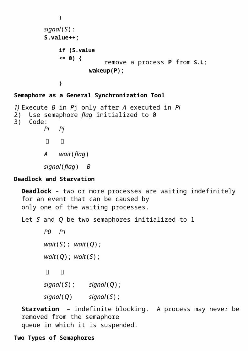
signal(S): S.value++;
if (S.value <= 0) {
remove a process P from S.L;
}
wakeup(P);
Semaphore as a General Synchronization Tool
1) Execute B in Pj only after A executed in Pi 2) Use semaphore flag initialized to 0 3) Code:
Pi
A
Pj
wait(flag)
signal(flag) B
Deadlock and Starvation
Deadlock – two or more processes are waiting indefinitely for an event that can be caused byonly one of the waiting processes.
Let S and Q be two semaphores initialized to 1
P0 P1
wait(S);
wait(Q);
wait(Q);
wait(S);
signal(S); signal(Q);
signal(Q) signal(S);
Starvation – indefinite blocking. A process may never be removed from the semaphorequeue in which it is suspended.
Two Types of Semaphores
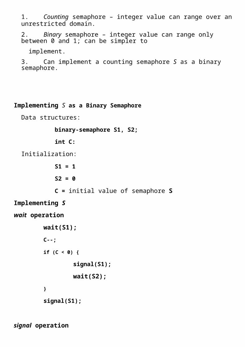
1. Counting semaphore – integer value can range over an unrestricted domain.
2. Binary semaphore – integer value can range only between 0 and 1; can be simpler to
implement.
3. Can implement a counting semaphore S as a binary semaphore.
Implementing S as a Binary Semaphore
Data structures:
binary-semaphore S1, S2;
int C:
Initialization:
S1 = 1
S2 = 0
C = initial value of semaphore S
Implementing S
wait operation
wait(S1);
C--;
if (C < 0) {
signal(S1);
wait(S2);
}
signal(S1);
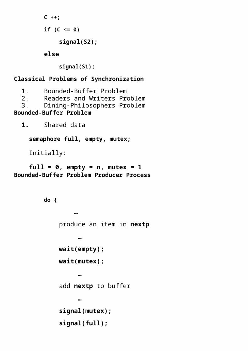
signal operation
wait(S1);

C ++;
if (C <= 0)
signal(S2);
else
signal(S1);
Classical Problems of Synchronization
1. Bounded-Buffer Problem 2. Readers and Writers Problem 3. Dining-Philosophers Problem
Bounded-Buffer Problem
1. Shared data
semaphore full, empty, mutex;
Initially:
full = 0, empty = n, mutex = 1 Bounded-Buffer Problem Producer Process
do {
…
produce an item in nextp
…
wait(empty);
wait(mutex);
…
add nextp to buffer
…
signal(mutex);
signal(full);
} while (1);
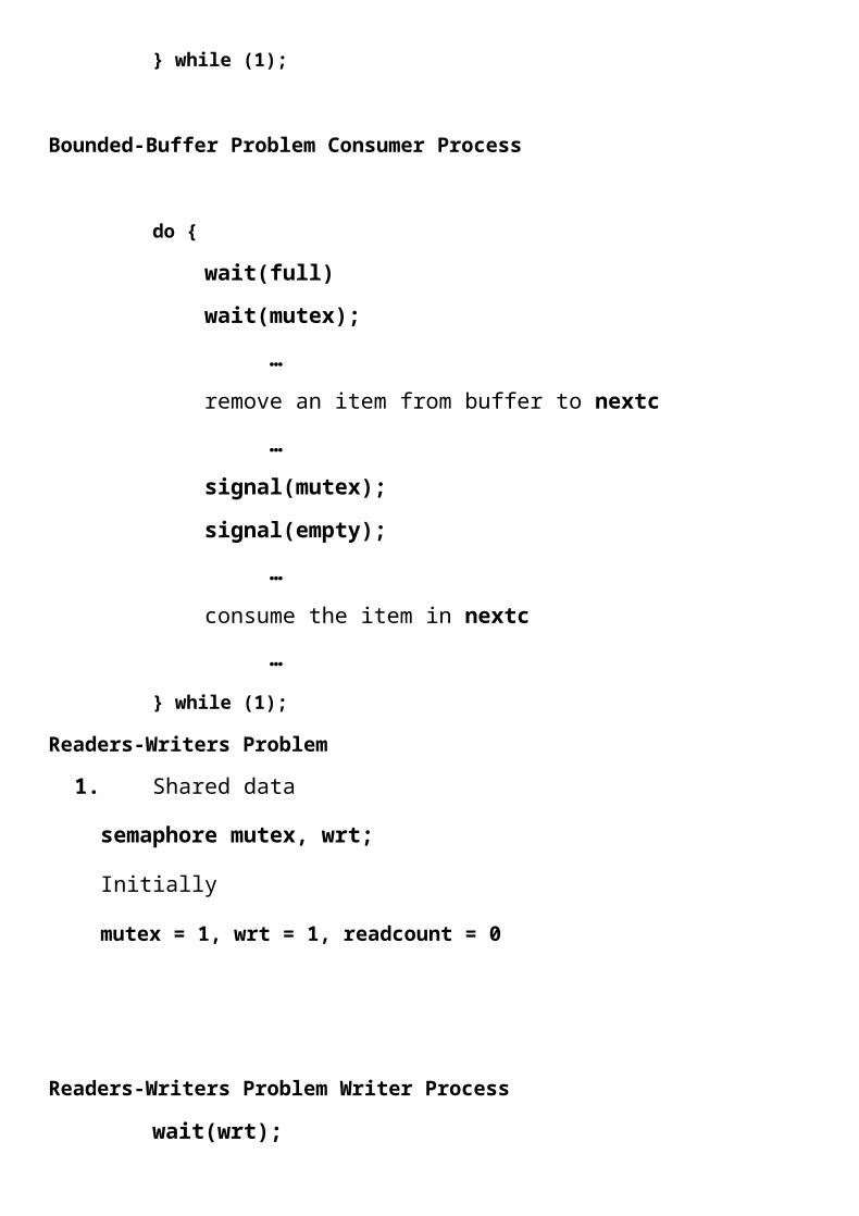
Bounded-Buffer Problem Consumer Process
do {
wait(full)
wait(mutex);
…
remove an item from buffer to nextc
…
signal(mutex);
signal(empty);
…
consume the item in nextc
…
} while (1);
Readers-Writers Problem
1. Shared data
semaphore mutex, wrt;
Initially
mutex = 1, wrt = 1, readcount = 0
Readers-Writers Problem Writer Process
wait(wrt);

…
writing is performed
…
signal(wrt);
Readers-Writers Problem Reader Process
wait(mutex);
readcount++;
if (readcount == 1)
wait(rt);
signal(mutex);
reading is performed
wait(mutex);
readcount--;
if (readcount == 0)
signal(wrt);
signal(mutex):
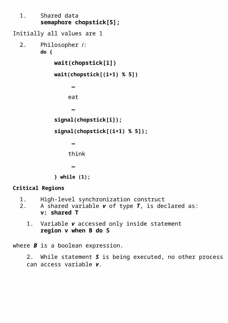
Dining-Philosophers Problem
1. Shared data semaphore chopstick[5];
Initially all values are 1
2. Philosopher i: do {
wait(chopstick[i])
wait(chopstick[(i+1) % 5])
…
eat
…
signal(chopstick[i]);
signal(chopstick[(i+1) % 5]);
…
think
…
} while (1);
Critical Regions
1. High-level synchronization construct 2. A shared variable v of type T, is declared as:
v: shared T
1. Variable v accessed only inside statement region v when B do S
where B is a boolean expression.
2. While statement S is being executed, no other process can access variable v.
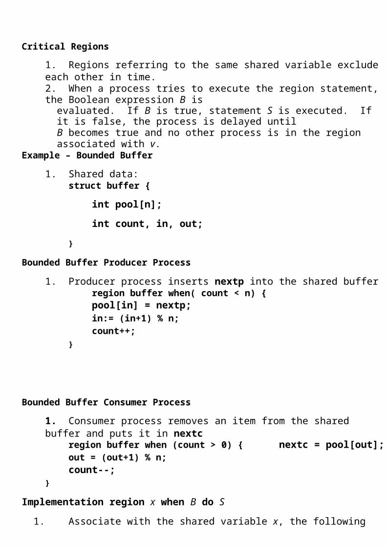
Critical Regions
1. Regions referring to the same shared variable exclude each other in time. 2. When a process tries to execute the region statement, the Boolean expression B is
evaluated. If B is true, statement S is executed. If it is false, the process is delayed untilB becomes true and no other process is in the region associated with v.
Example – Bounded Buffer
1. Shared data: struct buffer {
int pool[n];
int count, in, out;
}
Bounded Buffer Producer Process
1. Producer process inserts nextp into the shared buffer region buffer when( count < n) { pool[in] = nextp; in:= (in+1) % n;
count++;
}
Bounded Buffer Consumer Process
1. Consumer process removes an item from the shared buffer and puts it in nextc
}
region buffer when (count > 0) { out = (out+1) % n;
count--;
nextc = pool[out];
Implementation region x when B do S
1. Associate with the shared variable x, the following variables: i. semaphore mutex, first-delay, second-delay;
int first-count, second-count; 2. Mutually exclusive access to the critical section is provided by mutex.
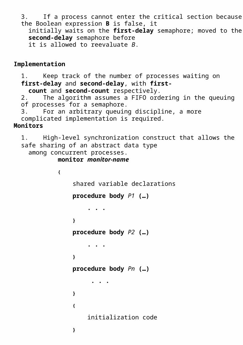
3. If a process cannot enter the critical section because the Boolean expression B is false, it
initially waits on the first-delay semaphore; moved to the second-delay semaphore beforeit is allowed to reevaluate B.
Implementation
1. Keep track of the number of processes waiting on first-delay and second-delay, with first-
count and second-count respectively. 2. The algorithm assumes a FIFO ordering in the queuing of processes for a semaphore. 3. For an arbitrary queuing discipline, a more complicated implementation is required.
Monitors
1. High-level synchronization construct that allows the safe sharing of an abstract data type
among concurrent processes. monitor monitor-name
{
shared variable declarations
procedure body P1 (…)
. . .
}
procedure body P2 (…)
. . .
}
procedure body Pn (…)
. . .
}
{
initialization code
}
}

1. To allow a process to wait within the monitor, a condition variable must be declared, as
condition x, y;

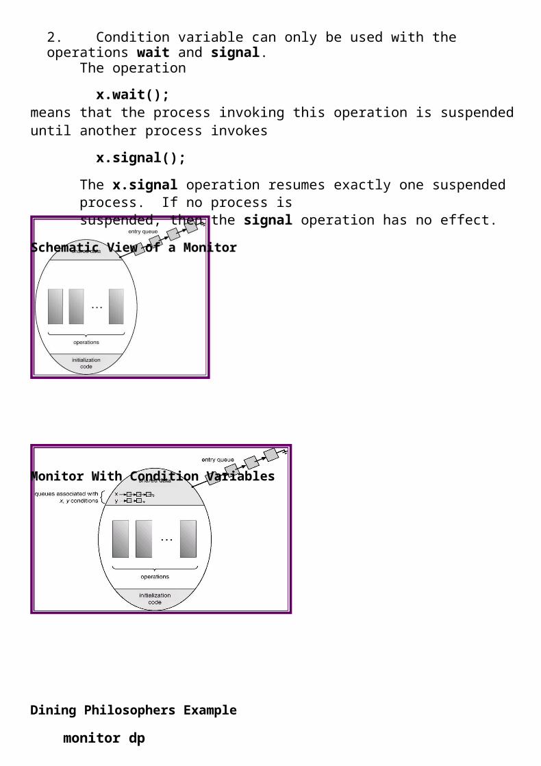
2. Condition variable can only be used with the operations wait and signal. The operation
x.wait(); means that the process invoking this operation is suspended until another process invokes
x.signal();
The x.signal operation resumes exactly one suspended process. If no process issuspended, then the signal operation has no effect.
Schematic View of a Monitor
Monitor With Condition Variables
Dining Philosophers Example
monitor dp
{
enum {thinking, hungry, eating} state[5];
condition self[5];
void pickup(int i)
void putdown(int i)
void test(int i)
void init() {
// following slides
// following slides
// following slides
}
}
for (int i = 0; i < 5; i++)
state[i] = thinking;
void pickup(int i) {
state[i] = hungry;
test[i];
if (state[i] != eating)
self[i].wait();
}
void putdown(int i) {
state[i] = thinking;
// test left and right neighbors
test((i+4) % 5);
test((i+1) % 5);
}
void test(int i) {
if ( (state[(I + 4) % 5] != eating) &&
(state[i] == hungry) &&
}
(state[(i + 1) % 5] != eating)) {
state[i] = eating;
self[i].signal();
}
Monitor Implementation Using Semaphores
1. Variables semaphore mutex; // (initially = 1)
semaphore next; // (initially = 0)
int next-count = 0;
2. Each external procedure F will be replaced by wait(mutex);
body of F;
if (next-count > 0)
signal(next)
else
signal(mutex);
3. Mutual exclusion within a monitor is ensured.
Monitor Implementation
1. For each condition variable x, we have: semaphore x-sem; // (initially = 0)
int x-count = 0;
2. The operation x.wait can be implemented as:
x-count++;
if (next-count > 0)
signal(next);
else
signal(mutex);
wait(x-sem);
x-count--;
3. The operation x.signal can be implemented as: if (x-count > 0) {
next-count++;
signal(x-sem);
wait(next);
next-count--;
}
Monitor Implementation
1. Conditional-wait construct: x.wait(c); a. c – integer expression evaluated when the wait operation is executed. b. value of c (a priority number) stored with the name of the process that is suspended. c. when x.signal is executed, process with smallest associated priority number is
resumed next. 2. Check two conditions to establish correctness of system:
a. User processes must always make their calls on the monitor in a correct sequence. b. Must ensure that an uncooperative process does not ignore the mutual-exclusion
gateway provided by the monitor, and try to access the shared resource directly, without using the access protocols.

Deadlocks
1. System Model 2. Deadlock Characterization 3. Methods for Handling Deadlocks 4. Deadlock Prevention 5. Deadlock Avoidance 6. Deadlock Detection 7. Recovery from Deadlock 8. Combined Approach to Deadlock Handling
The Deadlock Problem
1. A set of blocked processes each holding a resource and waiting to acquire a resource held
by another process in the set. 2. Example
a. System has 2 tape drives. b. P1 and P2 each hold one tape drive and each needs another one.
3. Example a. semaphores A and B, initialized to 1
P0
wait (A);
wait (B);
P1
wait(B)
wait(A)
Bridge Crossing Example
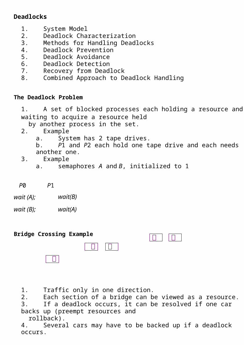
1. Traffic only in one direction. 2. Each section of a bridge can be viewed as a resource. 3. If a deadlock occurs, it can be resolved if one car backs up (preempt resources and
rollback). 4. Several cars may have to be backed up if a deadlock occurs. 5. Starvation is possible.
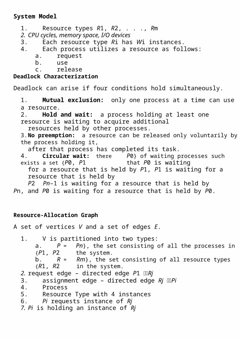
System Model
1. Resource types R1, R2, . . ., Rm 2. CPU cycles, memory space, I/O devices 3. Each resource type Ri has Wi instances. 4. Each process utilizes a resource as follows:
a. request b. use c. release
Deadlock Characterization
Deadlock can arise if four conditions hold simultaneously.
1. Mutual exclusion: only one process at a time can use a resource. 2. Hold and wait: a process holding at least one resource is waiting to acquire additional
resources held by other processes. 3. No preemption: a resource can be released only voluntarily by the process holding it,
after that process has completed its task. 4. Circular wait: there exists a set {P0, P1 P0} of waiting processes such that P0 is waiting
for a resource that is held by P1, P1 is waiting for a resource that is held by P2 Pn–1 is waiting for a resource that is held by
Pn, and P0 is waiting for a resource that is held by P0.
Resource-Allocation Graph
A set of vertices V and a set of edges E.
1. V is partitioned into two types: a. P = {P1, P2b. R = {R1, R2
Pn}, the set consisting of all the processes in the system. Rm}, the set consisting of all resource types in the system.
2. request edge – directed edge P1 Rj 3. assignment edge – directed edge Rj Pi4. Process 5. Resource Type with 4 instances 6. Pi requests instance of Rj7. Pi is holding an instance of Rj

Example of a ResourceAllocation Graph
Basic Facts
Resource AllocationGraph With A Deadlock
Resource AllocationGraph With A Cycle But
No Deadlock
1. If graph contains no cycles no deadlock. 2. If graph contains a cycle
a. if only one instance per resource type, then deadlock. b. if several instances per resource type, possibility of deadlock.
Methods for Handling Deadlocks
1. Ensure that the system will never enter a deadlock state. 2. Allow the system to enter a deadlock state and then recover. 3. Ignore the problem and pretend that deadlocks never occur in the system; used by most
operating systems, including UNIX. Deadlock Prevention
Restrain the ways request can be made.
1. Mutual Exclusion – not required for sharable resources; must hold for nonsharableresources.
2. Hold and Wait – must guarantee that whenever a process requests a resource, it does not
hold any other resources. a. Require process to request and be allocated all its resources before it begins
execution, or allow process to request resources only when the process has
none. b. Low resource utilization; starvation possible.
3. No Preemption – If a process that is holding some resources requests another resource that
cannot be immediately allocated to it, then all resources currently beingheld are released.
Preempted resources are added to the list of resources for which theprocess is waiting.
Process will be restarted only when it can regain its old resources, as well as
the new ones that it is requesting. 4. Circular Wait – impose a total ordering of all resource types, and require that each process
requests resources in an increasing order of enumeration. Deadlock Avoidance
Requires that the system has some additional a priori information available.
1. Simplest and most useful model requires that each process declare the maximum number
of resources of each type that it may need. 2. The deadlock-avoidance algorithm dynamically examines the resource-allocation state to
ensure that there can never be a circular-wait condition. 3. Resource-allocation state is defined by the number of available and allocated resources,
and the maximum demands of the processes. Safe State
1. When a process requests an available resource, system must decide if immediate allocation leaves the system in a safe state.
2. System is in safe state if there exists a safe sequence of all processes. 3. Sequence <P1, P2 Pn> is safe if for each Pi, the resources that Pi can still request
can be satisfied by currently available resources + resources held by all the Pj, with j<I.
a. If Pi resource needs are not immediately available, then Pi can wait until all Pj have
finished. b. When Pj is finished, Pi can obtain needed resources, execute, return allocated
resources, and terminate. c. When Pi terminates, Pi+1 can obtain its needed resources, and so on.
Basic Facts
1. If a system is in safe state no deadlocks. 2. If a system is in unsafe state possibility of deadlock. 3. Avoidance ensure that a system will never enter an unsafe state.
Safe, Unsafe , Deadlock State
Resource-Allocation Graph Algorithm
1. Claim edge Pi Rj indicated that process Pj may request resource Rj; represented by a
dashed line. 2. Claim edge converts to request edge when a process requests a resource. 3. When a resource is released by a process, assignment edge reconverts to a claim edge. 4. Resources must be claimed a priori in the system.
Resource-Allocation Graph For Deadlock Avoidance
Unsafe State In Resource-Allocation Graph
Banker’s lgorithm
1. Multiple instances. 2. Each process must a priori claim maximum use. 3. When a process requests a resource it may have to wait. 4. When a process gets all its resources it must return them in a finite amount of time. Data Structures for the Banker’s lgorithm
Let n = number of processes, and m = number of resources types.
1. Available: Vector of length m. If available [j] = k, there are k instances of resource type Rj
available. 2. Max: n x m matrix. If Max [i,j] = k, then process Pi may request at most k instances of
resource type Rj. 3. Allocation: n x m matrix. If Allocation[i,j] = k then Pi is currently allocated k instances of Rj.4. Need: n x m matrix. If Need[i,j] = k, then Pi may need k more instances of Rj to complete its
task. 5. Need [i,j] = Max[i,j] – Allocation [i,j].
Safety Algorithm
1.Let Work and Finish be vectors of length m and n, respectively. Initialize:
Work = Available
Finish [i] = false for i - 1 3
2.Find and i such that both:
(a) Finish [i] = false
(b) Needi Work
n.
If no such i exists, go to step 4.
3.Work = Work + AllocationiFinish[i] = truego to step 2.
4.If Finish [i] == true for all i, then the system is in a safe state.
Resource-Request Algorithm for Process Pi
Request = request vector for process Pi. If Requesti [j] = k then process Pi wants k instancesof resource type Rj.
1.If Requesti Needi go to step 2. Otherwise, raise error condition, since process hasexceeded its maximum claim.
2.If Requesti Available, go to step 3. Otherwise Pi must wait, since resources are notavailable.
3.Pretend to allocate requested resources to Pi by modifying the state as follows:
Available = Available = Requesti;
Allocationi = Allocationi + Requesti;
Needi = Needi – Requesti;;
• If safe the resources are allocated to Pi. • If unsafe Pi must wait, and the old resource-allocation state is restored
Example of Banker’s lgorithm
1. 5 processes P0 through P4; 3 resource types A(10 instances), B (5instances, and C (7 instances).
2. Snapshot at time T0: Allocation Max Available
A B C A B C A B C
P0 0 1 0 7 5 3 3 3 2
P1 2 0 0 3 2 2
P2 3 0 2 9 0 2
P3 2 1 1 2 2 2
P4 0 0 2 4 3 3
3. The content of the matrix. Need is defined to be Max – Allocation. Need
A B C
P0 7 4 3
P1 1 2 2
P2 6 0 0
P3 0 1 1
P4 4 3 1
4. The system is in a safe state since the sequence < P1, P3, P4, P2, P0> satisfies safety criteria.
Example P1 Request (1,0,2) (Cont.)
1. Check that Request Available (that is, (1,0,2) (3,3,2) true. Allocation Need Available
A B C A B C A B C
P0 0 1 0 7 4 3 2 3 0
P1 3 0 2 0 2 0
P2 3 0 1 6 0 0
P3 2 1 1 0 1 1
P4 0 0 2 4 3 1
1. Executing safety algorithm shows that sequence <P1, P3, P4, P0, P2> satisfies safetyrequirement.
2. Can request for (3,3,0) by P4 be granted? 3. Can request for (0,2,0) by P0 be granted?
Deadlock Detection
1. Allow system to enter deadlock state 2. Detection algorithm 3. Recovery scheme
Single Instance of Each Resource Type
1. Maintain wait-for graph a. Nodes are processes. b. Pi Pj if Pi is waiting for Pj.
2. Periodically invoke an algorithm that searches for a cycle in the graph. 3. An algorithm to detect a cycle in a graph requires an order of n2 operations, where n is the
number of vertices in the graph. Resource-Allocation Graph and Wait-for Graph
a. Resource-Allocation Graph b.Corresponding wait-for graph
Several Instances of a Resource Type
1. Available: A vector of length m indicates the number of available resources of each type. 2. Allocation: An n x m matrix defines the number of resources of each type currently
allocated to each process. 3. Request: An n x m matrix indicates the current request of each process. If Request [ij] = k,
then process Pi is requesting k more instances of resource type. Rj. Detection Algorithm
1. Let Work and Finish be vectors of length m and n, respectively Initialize:
(a) Work = Available
(b) For i = 1 2 n, if Allocationi 0, then Finish[i] = false;otherwise, Finish[i] = true.
2. Find an index i such that both:
(a) Finish[i] == false
(b) Requesti Work
If no such i exists, go to step 4.
3. Work = Work + AllocationiFinish[i] = truego to step 2.
4. If Finish[i] == false, for some i, 1 i n, then the system is in deadlock state. Moreover, if
Finish[i] == false, then Pi is deadlocked.

Algorithm requires an order of O(m x n2) operations to detect whether the system is in
deadlocked state.
Example of Detection Algorithm
1.Five processes P0 through P4; three resource types A (7 instances), B (2 instances), and C (6 instances).
2.Snapshot at time T0:
Allocation Request
A B C A B C A B C
Available
P0 0 1 0 0 0 0 0 0 0
P1 2 0 0 2 0 2
P2 3 0 3 0 0 0
P3 2 1 1 1 0 0
P4 0 0 2 0 0 2
3.Sequence <P0, P2, P3, P1, P4> will result in Finish[i] = true for all i.
4.P2 requests an additional instance of type C.
Request
A B C
P0 0 0 0
P1 2 0 1
P2 0 0 1
P3 1 0 0
P4 0 0 2
5.State of system
o Can reclaim resources held by process P0, but insufficient resources to fulfill other
processes; requests.

o Deadlock exists, consisting of processes P1, P2, P3, and P4.

Detection-Algorithm Usage
1. When, and how often, to invoke depends on: a. How often a deadlock is likely to occur? b. How many processes will need to be rolled back?
i. one for each disjoint cycle 2. If detection algorithm is invoked arbitrarily, there may be many cycles in the resource
graph and so we would not be able to tell which of the many deadlocked processes“caused” the deadlock
Recovery from Deadlock: Process Termination
1. Abort all deadlocked processes. 2. Abort one process at a time until the deadlock cycle is eliminated. 3. In which order should we choose to abort?
a. Priority of the process. b. How long process has computed, and how much longer to completion. c. Resources the process has used. d. Resources process needs to complete. e. How many processes will need to be terminated. f. Is process interactive or batch?
Recovery from Deadlock: Resource Preemption
1. Selecting a victim – minimize cost. 2. Rollback – return to some safe state, restart process for that state. 3. Starvation – same process may always be picked as victim, include number of rollback in
cost factor Combined Approach to Deadlock Handling
1. Combine the three basic approaches a. prevention b. avoidance c. detection
allowing the use of the optimal approach for each of resources in the system.
2. Partition resources into hierarchically ordered classes.
3. Use most appropriate technique for handling deadlocks within each class.

UNIT II-PROCESS SCHEDULING AND SYNCHRONIZATION
PART – A (2 MARKS)
1. Define CPU scheduling.
2. What is preemptive and no preemptive scheduling?
3. What is a Dispatcher?
4. What is dispatch latency?
5. What are the various scheduling criteria for CPU scheduling?
6. Define throughput?
7. What is turnaround time?
8. Define race condition.
9. What is critical section problem?
10.What are the requirements that a solution to the critical section problem must satisfy?
11.Define entry section and exit section.
12.Give two hardware instructions and their definitions which can be used for implementing mutual
exclusion.
• TestAndSet
boolean TestAndSet (boolean &target)
{
boolean rv = target;
target = true;
return rv;
}
• Swap
void Swap (boolean &a, boolean &b)
{
boolean temp = a;
a = b;
b = temp;
}
13.What is semaphores?
14. Define busy waiting and spin lock.
15. Define deadlock.
16. What is the sequence in which resources may be utilized?
17. What are conditions under which a deadlock situation may arise?
18. What is a resource-allocation graph?
19. Define request edge and assignment edge.
20. What are the methods for handling deadlocks?
21. Define deadlock prevention.
22. Define deadlock avoidance.
23. What are a safe state and an unsafe state?
24. What is banker’s algorithm?
PART B
1. Write about the various CPU scheduling algorithms. (16)
2. Consider the following set of processes, with the length of the CPU-burst time in given
ms(16)
Process Burst Time Priority
P1 10 3
P2 1 1
P3 2 3
P4 1 4
P5 5 2
The processes are assumed to have arrived in the order P1, P2, P3, P4,P5 all at time 0.
a. Draw four Gants charts illustrating the execution of these process using FCFS,SJF,a
non preemptive priority(a smaller priority number implies a higher priority) ,and
RR(quantum=1)scheduling.
b. What is the turn around time of each process for each of the scheduling algorithms in
part a?
c. What is the waiting time of each process for each of the scheduling algorithms in part
a?
d. Which of the schedules in part a result in the minimal average waiting time(over all
process)? (16)
3. Write notes about multiple-processor scheduling and real-time scheduling. (16)
4. What is critical section problem and explain two process solutions and multiple process
solutions? (16)
5. Explain what semaphores are, their usage, implementation given to avoid busy waiting and
binary semaphores. (16)
6. Explain the classic problems of synchronization. (16)
7. Write about critical regions and monitors. (16)
8. Give a detailed description about deadlocks and its characterization (16)
9. Explain about the methods used to prevent deadlocks (16)
10. Write in detail about deadlock avoidance. (16)
11. Explain the Banker's algorithm for deadlock avoidance. (16)
12. Give an account about deadlock detection. (16)
13. What are the methods involved in recovery from deadlocks? (16)

UNIT III STORAGE MANAGEMENT
Memory management – Background – Swapping – Contiguous memory allocation – Paging – Segmentation – Segmentation with paging – Virtual memory – Background – Demand paging – Process creation – Page replacement – Allocation of frames – Thrashing – Case study – Memory management in linux .
UNIT-III
Memory Management
1. Background 2. Swapping 3. Contiguous Allocation 4. Paging 5. Segmentation 6. Segmentation with Paging
Background
1. Program must be brought into memory and placed within a process for it to be run. 2. Input queue – collection of processes on the disk that are waiting to be brought into memory to run the program. 3. User programs go through several steps before being run.
Binding of Instructions and Data to Memory
Address binding of instructions and data to memory addresses can happen at three different stages.
1. Compile time: If memory location known a priori, absolute code can be generated; must recompile code if starting location changes.
2. Load time: Must generate relocatable code if memory location is not known at compile time. 3. Execution time: Binding delayed until run time if the process can be moved during its execution from one memory segment to
another. Need hardware support for address maps (e.g., base and limit registers).
Multistep Processing of a User Program
Logical vs. Physical Address Space
1. The concept of a logical address space that is bound to a separate physical address space is central to proper memory management.
a. Logical address – generated by the CPU; also referred to as virtual address. b. Physical address – address seen by the memory unit.
2. Logical and physical addresses are the same in compile-time and load-time address-binding schemes; logical (virtual) and physical addresses differ in execution-time address-binding scheme.
Memory-Management Unit (MMU)
1. Hardware device that maps virtual to physical address. 2. In MMU scheme, the value in the relocation register is added to every address generated by a user process at the time it is sent
to memory. 3. The user program deals with logical addresses; it never sees the real physical addresses.
Dynamic relocation using a relocation register
Dynamic Loading
1. Routine is not loaded until it is called 2. Better memory-space utilization; unused routine is never loaded. 3. Useful when large amounts of code are needed to handle infrequently occurring cases. 4. No special support from the operating system is required implemented through program design.
Dynamic Linking
1. Linking postponed until execution time. 2. Small piece of code, stub, used to locate the appropriate memory-resident library routine. 3. Stub replaces itself with the address of the routine, and executes the routine. 4. Operating system needed to check if routine is in processes’ memory address 5. Dynamic linking is particularly useful for libraries
Overlays
1. Keep in memory only those instructions and data that are needed at any given time. 2. Needed when process is larger than amount of memory allocated to it. 3. Implemented by user, no special support needed from operating system, programming design of overlay structure is complex
Overlays for a Two-Pass Assembler
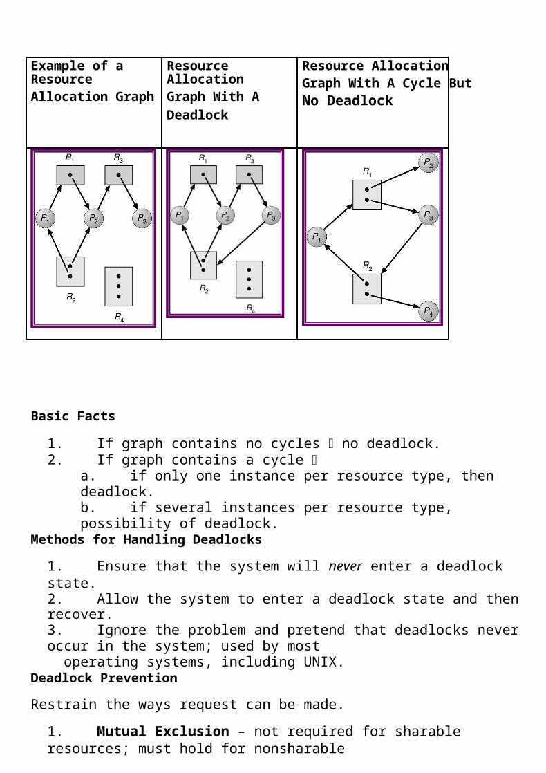
Swapping
1. A process can be swapped temporarily out of memory to a backing store, and then brought back into memory for continued execution.
2. Backing store – fast disk large enough to accommodate copies of all memory images for all users; must provide direct access to these memory images.
3. Roll out, roll in – swapping variant used for priority-based scheduling algorithms; lower-priority process is swapped out so higher-priority process can be loaded and executed.
4. Major part of swap time is transfer time; total transfer time is directly proportional to the amount of memory swapped. 5. Modified versions of swapping are found on many systems, i.e., UNIX, Linux, and Windows.

Contiguous Allocation
1. Main memory usually into two partitions: a. Resident operating system, usually held in low memory with interrupt vector. b. User processes then held in high memory.
2. Single-partition allocation a. Relocation-register scheme used to protect user processes from each other, and from changing operating-system code
and data. b. Relocation register contains value of smallest physical address; limit register contains range of logical addresses – each
logical address must be less than the limit register. Hardware Support for Relocation and Limit Registers
Contiguous Allocation (Cont.)
1. Multiple-partition allocation a. Hole – block of available memory; holes of various size are scattered throughout memory. b. When a process arrives, it is allocated memory from a hole large enough to accommodate it. c. Operating system maintains information about:
a) allocated partitions b) free partitions (hole) Dynamic Storage-Allocation Problem
How to satisfy a request of size n from a list of free holes.
1. First-fit: Allocate the first hole that is big enough. 2. Best-fit: Allocate the smallest hole that is big enough; must search entire list, unless ordered by size. Produces the smallest
leftover hole. 3. Worst-fit: Allocate the largest hole; must also search entire list. Produces the largest leftover hole.
First-fit and best-fit better than worst-fit in terms of speed and storage utilization.
Fragmentation
1. External Fragmentation – total memory space exists to satisfy a request, but it is not contiguous. 2. Internal Fragmentation – allocated memory may be slightly larger than requested memory; this size difference is memory
internal to a partition, but not being used. 3. Reduce external fragmentation by compaction
a. Shuffle memory contents to place all free memory together in one large block. b. Compaction is possible only if relocation is dynamic, and is done at execution time. c. I/O problem
i. Latch job in memory while it is involved in I/O. ii. Do I/O only into OS buffers.
Paging
1. Logical address space of a process can be noncontiguous; process is allocated physical memory whenever the latter is available. 2. Divide physical memory into fixed-sized blocks called frames (size is power of 2, between 512 bytes and 8192 bytes). 3. Divide logical memory into blocks of same size called pages. 4. Keep track of all free frames. 5. To run a program of size n pages, need to find n free frames and load program. 6. Set up a page table to translate logical to physical addresses.

7. Internal fragmentation.
Address Translation Scheme
1. Address generated by CPU is divided into: a. Page number (p) – used as an index into a page table which contains base address of each page in physical memory. b. Page offset (d) – combined with base address to define the physical memory address that is sent to the memory unit.
Address Translation Architecture
Paging Example
Free Frames
Implementation of Page Table
1. Page table is kept in main memory. 2. Page-table base register (PTBR) points to the page table. 3. Page-table length register (PRLR) indicates size of the page table. 4. In this scheme every data/instruction access requires two memory accesses. One for the page table and one for the
data/instruction. 5. The two memory access problem can be solved by the use of a special fast-lookup hardware cache called associative memory
or translation look-aside buffers (TLBs) Associative Memory
1. Associative memory – parallel search Address translation (A´, A´´)
a. If A´ is in associative register, get frame # out. b. Otherwise get frame # from page table in memory
Paging Hardware With TLB
Effective Access Time

Memory Protection
1. Memory protection implemented by associating protection bit with each frame. 2. Valid-invalid bit attached to each entry in the page table:
a. “valid” indicates that the associated page is in the process’ logical address space and is thus a legal page b. “invalid” indicates that the page is not in the process’ logical address space
Valid (v) or Invalid (i) Bit In A Page Table
Page Table Structure
1. Hierarchical Paging 2. Hashed Page Tables 3. Inverted Page Tables
Hierarchical Page Tables
1. Break up the logical address space into multiple page tables. 2. A simple technique is a two-level page table.
Two-Level Paging Example
1. A logical address (on 32-bit machine with 4K page size) is divided into: a. a page number consisting of 20 bits. b. a page offset consisting of 12 bits.
2. Since the page table is paged, the page number is further divided into: a. a 10-bit page number. b. a 10-bit page offset.
where pi is an index into the outer page table, and p2 is the displacement within the page of the outer page table.
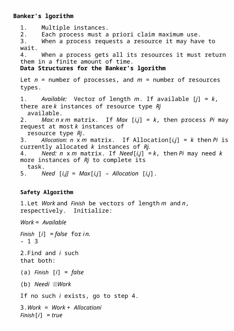
Two-Level Page-Table Scheme
Address-Translation Scheme
1. Address-translation scheme for a two-level 32-bit paging architecture
Hashed Page Tables
2. Common in address spaces > 32 bits.
3. The virtual page number is hashed into a page table. This page table contains a chain of elements hashing to the same location.
4. Virtual page numbers are compared in this chain searching for a match. If a match is found, the corresponding physical frame is extracted.
Hashed Page Table
Inverted Page Table
1. One entry for each real page of memory.
2. Entry consists of the virtual address of the page stored in that real memory location, with information about the process that owns that page.
3. Decreases memory needed to store each page table, but increases time needed to search the table when a page reference occurs.
4. Use hash table to limit the search to one — or at most a few — page-table entries.
Shared Pages
1. Shared code a. One copy of read-only (reentrant) code shared among processes (i.e., text editors, compilers, window systems). b. Shared code must appear in same location in the logical address space of all processes.
2. Private code and data a. Each process keeps a separate copy of the code and data. b. The pages for the private code and data can appear anywhere in the logical address space.
Segmentation
1. Memory-management scheme that supports user view of memory. 2. A program is a collection of segments. A segment is a logical unit such as:
main program,procedure, function,method,object,local variables, global variables,common block,stack,symbol table, arrays
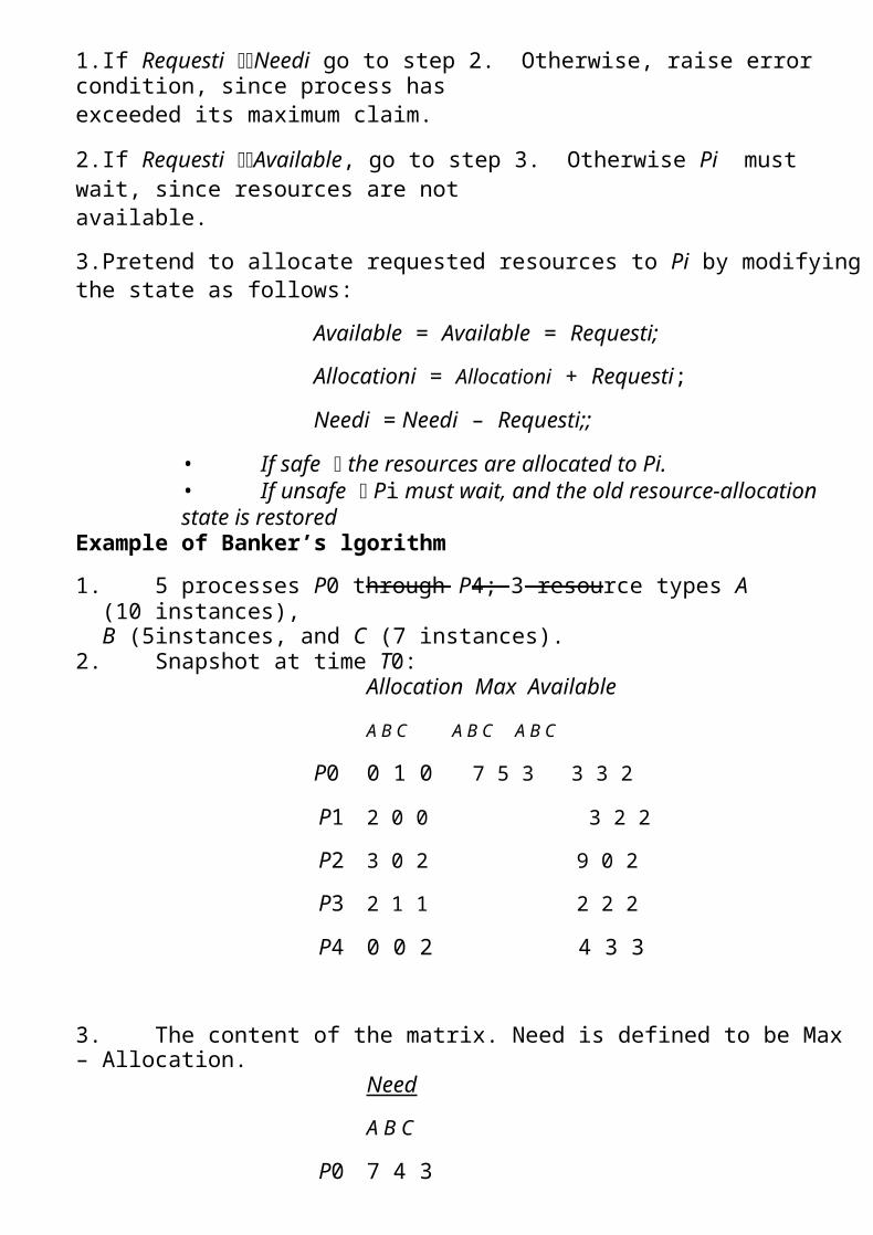
User’s View of a Program
Segmentation Architecture
Logical address consists of a two tuple: o <segment-number, offset>,
Segment table – maps two-dimensional physical addresses; each table entry has: base – contains the starting physical address where the segments reside in memory limit – specifies the length of the segment Segment-table base register (STBR) points to the segment table’s location in memory Segment-table length register (STLR) indicates number of segments used by a program; segment number s is legal if s < STLR
Protection With each entry in segment table associate: validation bit = 0 illegal segment read/write/execute privileges Protection bits associated with segments; code sharing occurs at segment level Since segments vary in length, memory allocation is a dynamic storage-allocation
problem
A segmentation example is shown in the following diagram. Segmentation Hardware

Example of Segmentation
Virtual Memory
1. Background 2. Demand Paging 3. Process Creation 4. Page Replacement 5. Allocation of Frames 6. Thrashing 7. Operating System Examples
Background
1. Virtual memory – separation of user logical memory from physical memory. a. Only part of the program needs to be in memory for execution. b. Logical address space can therefore be much larger than physical address space. c. Allows address spaces to be shared by several processes. d. Allows for more efficient process creation.
2. Virtual memory can be implemented via: a. Demand paging b. Demand segmentation
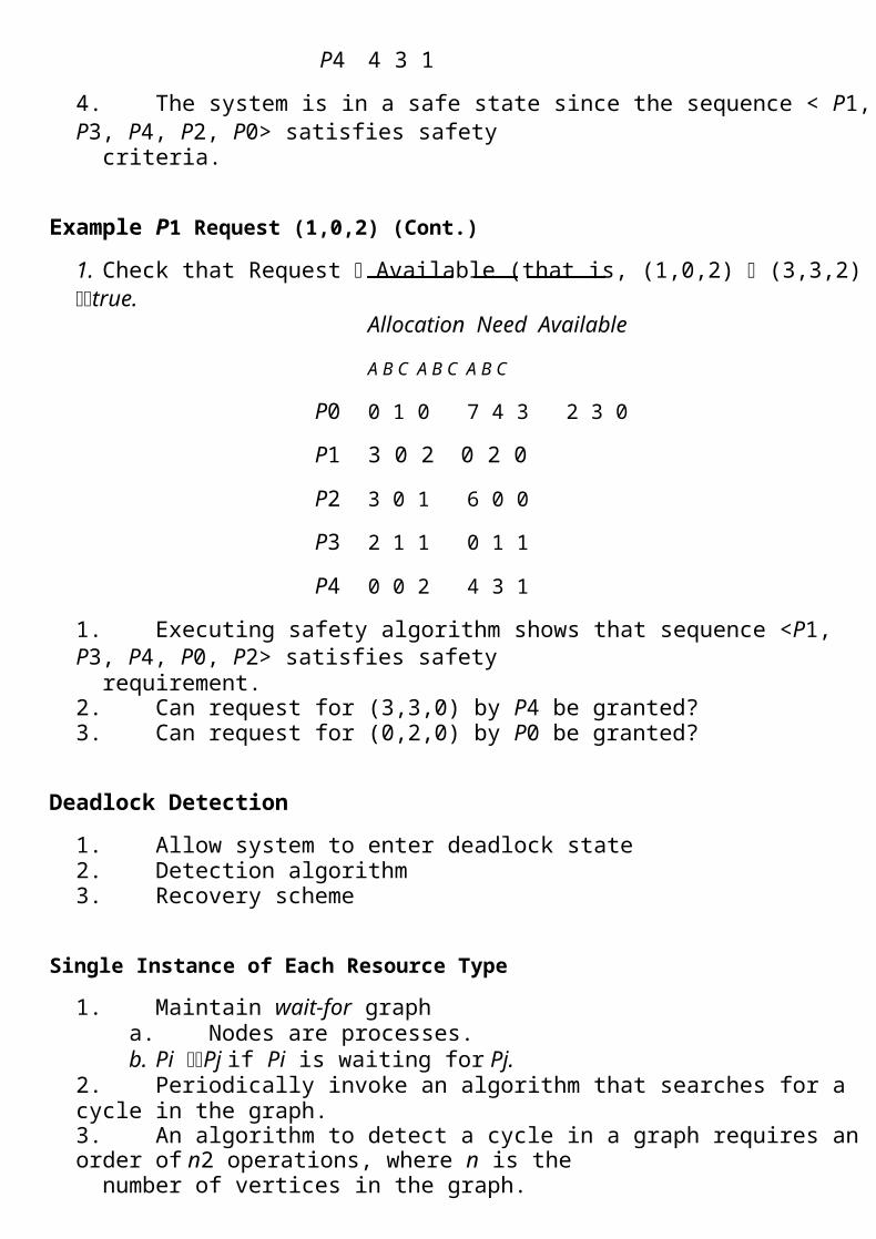
Virtual Memory That is Larger Than Physical Memory
Demand Paging
1. Bring a page into memory only when it is needed. a. Less I/O needed b. Less memory needed c. Faster response d. More users
2. Page is needed reference to it a. invalid reference abort b. not-in-memory bring to memory
Transfer of a Paged Memory to Contiguous Disk Space
Valid-Invalid Bit
1. With each page table entry a valid–invalid bit is associated (1 in-memory, 0 not-in-memory)
2. Initially valid–invalid but is set to 0 on all entries. 3. Example of a page table snapshot. 4. During address translation, if valid–invalid bit in page table entry is 0 page fault.

Page Table When Some Pages Are Not in Main Memory
Page Fault
1. If there is ever a reference to a page, first reference will trap to OS page fault
2. OS looks at another table to decide: a. Invalid reference abort. b. Just not in memory.
3. Get empty frame. 4. Swap page into frame. 5. Reset tables, validation bit = 1. 6. Restart instruction: Least Recently Used
a. block move b. auto increment/decrement location
Steps in Handling a Page Fault
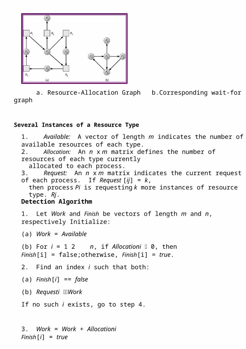
What happens if there is no free frame?
1. Page replacement – find some page in memory, but not really in use, swap it out. a. algorithm b. performance – want an algorithm which will result in minimum number of page faults.
2. Same page may be brought into memory several times.
Performance of Demand Paging
1. Page Fault Rate 0 p 1.0 a. if p = 0 no page faults b. if p = 1, every reference is a fault
2. Effective Access Time (EAT) EAT = (1 – p) x memory access
+ p (page fault overhead
+ [swap page out ]
+ swap page in
+ restart overhead)
Demand Paging Example
1. Memory access time = 1 microsecond 2. 50% of the time the page that is being replaced has been modified and therefore needs to be swapped out. 3. Swap Page Time = 10 msec = 10,000 msec
EAT = (1 – p) x 1 + p (15000)
1 + 15000P (in msec)
Process Creation
1. Virtual memory allows other benefits during process creation: - Copy-on-Write
- Memory-Mapped Files
Copy-on-Write
2. Copy-on-Write (COW) allows both parent and child processes to initially share the same pages in memory.
If either process modifies a shared page, only then is the page copied.
3. COW allows more efficient process creation as only modified pages are copied.
4. Free pages are allocated from a pool of zeroed-out pages.
Memory-Mapped Files
1. Memory-mapped file I/O allows file I/O to be treated as routine memory access by mapping a disk block to a page in memory.
2. A file is initially read using demand paging. A page-sized portion of the file is read from the file system into a physical page.Subsequent reads/writes to/from the file are treated as ordinary memory accesses.
3. Simplifies file access by treating file I/O through memory rather than read() write() system calls.
4. Also allows several processes to map the same file allowing the pages in memory to be shared.
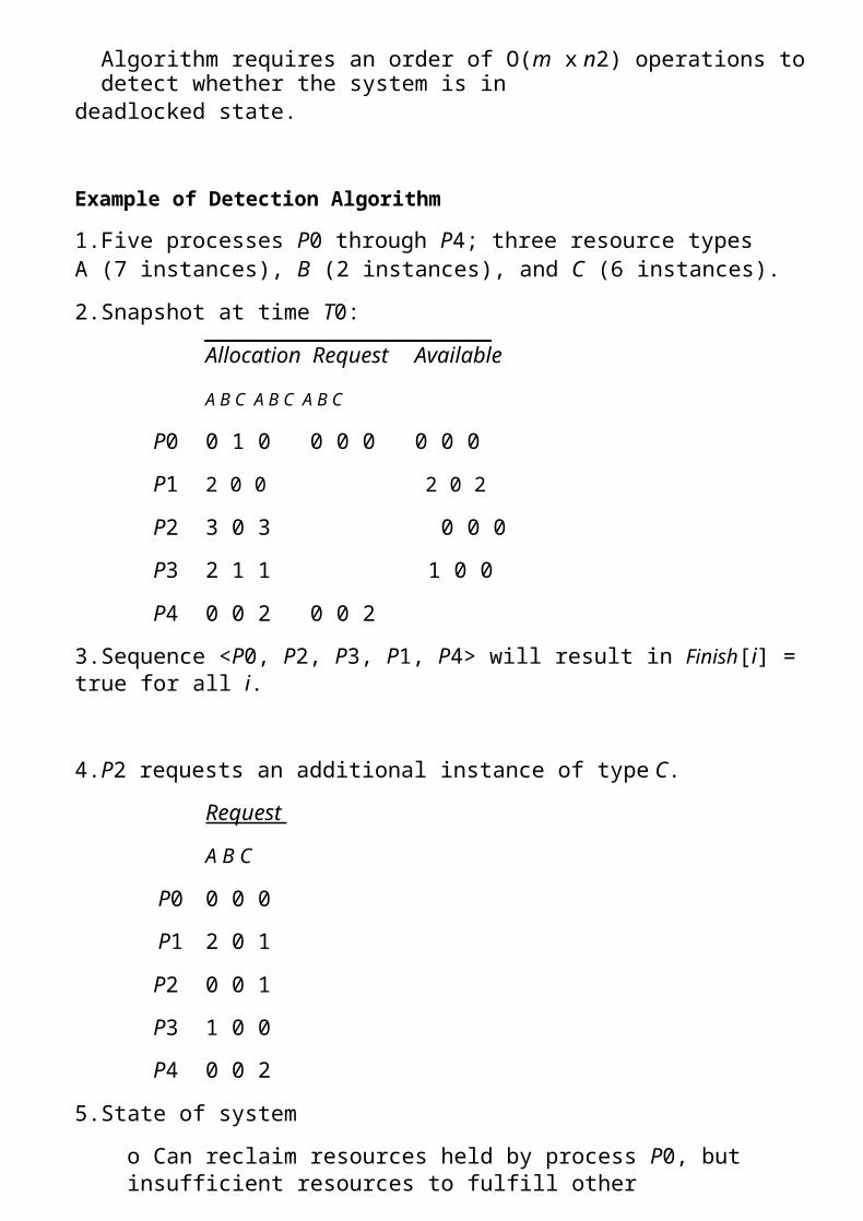
Memory Mapped Files
Page Replacement
1. Prevent over-allocation of memory by modifying page-fault service routine to include page replacement. 2. Use modify (dirty) bit to reduce overhead of page transfers – only modified pages are written to disk. 3. Page replacement completes separation between logical memory and physical memory – large virtual memory can be provided
on a smaller physical memory.
Need For Page Replacement
Basic Page Replacement
1. Find the location of the desired page on disk. 2. Find a free frame:
- If there is a free frame, use it. - If there is no free frame, use a page replacement algorithm to select a victim frame.
3. Read the desired page into the (newly) free frame. Update the page and frame tables. 4. Restart the process.
Page Replacement
Page Replacement Algorithms
1. Want lowest page-fault rate. 2. Evaluate algorithm by running it on a particular string of memory references (reference string) and computing the number of
page faults on that string. 3. In all our examples, the reference string is
1, 2, 3, 4, 1, 2, 5, 1, 2, 3, 4, 5.
Graph of Page Faults Versus The Number of Frames
First-In-First-Out (FIFO) Algorithm
1. Reference string: 1, 2, 3, 4, 1, 2, 5, 1, 2, 3, 4, 5 2. 3 frames (3 pages can be in memory at a time per process) 3. 4 frames
4. FIFO Replacement – Belady’s nomaly a. more frames less page faults

FIFO Page Replacement
FIFO Illustrating Belady’s namoly
Optimal Algorithm
1. Replace page that will not be used for longest period of time. 2. 4 frames example
1, 2, 3, 4, 1, 2, 5, 1, 2, 3, 4, 5
Optimal Page Replacement
Least Recently Used (LRU) Algorithm
1. Reference string: 1, 2, 3, 4, 1, 2, 5, 1, 2, 3, 4, 5
2. Counter implementation a. Every page entry has a counter; every time page is referenced through this entry, copy the clock into the counter. b. When a page needs to be changed, look at the counters to determine which are to change.
LRU Page Replacement

1. Stack implementation – keep a stack of page numbers in a double link form: a. Page referenced:
i. move it to the top ii. requires 6 pointers to be changed
b. No search for replacement
Use Of A Stack to Record The Most Recent Page References
LRU Approximation Algorithms
1. Reference bit a. With each page associate a bit, initially = 0 b. When page is referenced bit set to 1. c. Replace the one which is 0 (if one exists). We do not know the order, however.
2. Second chance a. Need reference bit. b. Clock replacement. c. If page to be replaced (in clock order) has reference bit = 1. then:
i. set reference bit 0. ii. leave page in memory. iii. replace next page (in clock order), subject to same rules.
Second-Chance (clock) Page-Replacement Algorithm
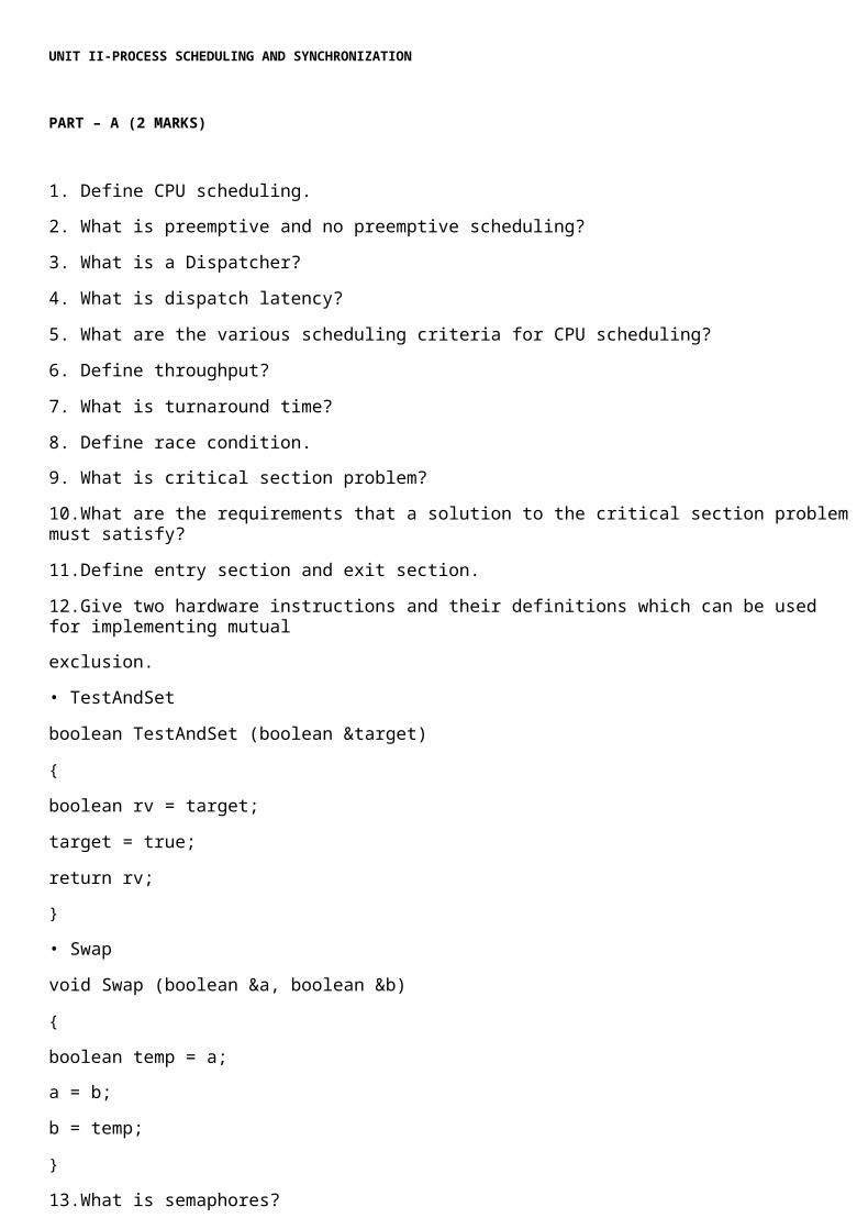
Counting Algorithms
1. Keep a counter of the number of references that have been made to each page. 2. LFU Algorithm: replaces page with smallest count. 3. MFU Algorithm: based on the argument that the page with the smallest count was probably just brought in and has yet to be
used. Allocation of Frames
1. Each process needs minimum number of pages. 2. Example: IBM 370 – 6 pages to handle SS MOVE instruction:
a. instruction is 6 bytes, might span 2 pages. b. 2 pages to handle from. c. 2 pages to handle to.
3. Two major allocation schemes. a. fixed allocation b. priority allocation
Fixed Allocation
1. Equal allocation – e.g., if 100 frames and 5 processes, give each 20 pages. 2. Proportional allocation – Allocate according to the size of process. 3.
sisize of process pi
S si
m total number of frames
ai allocation for p
i s
iS
m
m 64
si 10
s2127
10
Priority Allocation
1. Use a proportional allocation scheme using priorities rather than size. 2. If process Pi generates a page fault,
a. select for replacement one of its frames. b. select for replacement a frame from a process with lower priority number.
Global vs. Local Allocation
1. Global replacement – process selects a replacement frame from the set of all frames; one process can take a frame from another.
2. Local replacement – each process selects from only its own set of allocated frames. Thrashing
1. If a process does not have “enough” pages the page-fault rate is very high. This leads to: a. low CPU utilization. b. operating system thinks that it needs to increase the degree of multiprogramming. c. another process added to the system.
2. Thrashing a process is busy swapping pages in and out.
1. Why does paging work? Locality model
a. Process migrates from one locality to another. b. Localities may overlap.
2. Why does thrashing occur? size of locality > total memory size
Working-Set Model
1. working-set window a fixed number of page references Example: 10,000 instruction
2. WSSi (working set of Process Pi) = total number of pages referenced in the most recent (varies in time)
a. if too small will not encompass entire locality. b. if too large will encompass several localities. c. if = will encompass entire program.
3. D = WSSi total demand frames 4. if D > m Thrashing 5. Policy if D > m, then suspend one of the processes.

Keeping Track of the Working Set
1. Approximate with interval timer + a reference bit 2. Example: = 10,000
a. Timer interrupts after every 5000 time units. b. Keep in memory 2 bits for each page. c. Whenever a timer interrupts copy and sets the values of all reference bits to 0. d. If one of the bits in memory = 1 page in working set.
3. Why is this not completely accurate? 4. Improvement = 10 bits and interrupt every 1000 time units.
Page-Fault Frequency Scheme
1. Establish “acceptable” page-fault rate. a. If actual rate too low, process loses frame. b. If actual rate too high, process gains frame.
Other Considerations
1. Prepaging 2. Page size selection
a. fragmentation b. table size c. I/O overhead d. locality
3. TLB Reach - The amount of memory accessible from the TLB. 4. TLB Reach = (TLB Size) X (Page Size) 5. Ideally, the working set of each process is stored in the TLB. Otherwise there is a high degree of page faults.
Increasing the Size of the TLB
1. Increase the Page Size. This may lead to an increase in fragmentation as not all applications require a large page size. 2. Provide Multiple Page Sizes. This allows applications that require larger page sizes the opportunity to use them without an
increase in fragmentation.
Other Considerations (Cont.)
1. Program structure a. int A[][] = new int[1024][1024];
b. Each row is stored in one page
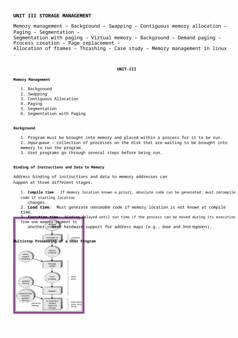
c. Program 1 for (j = 0; j < A.length; j++) for (i = 0; i < A.length; i++)
A[i,j] = 0; 1024 x 1024 page faults
d. Program 2
1024 page faults
for (i = 0; i < A.length; i++)
for (j = 0; j < A.length; j++) A[i,j] = 0;
1. I/O Interlock – Pages must sometimes be locked into memory.
2. Consider I/O. Pages that are used for copying a file from a device must be locked from being selected foreviction by a page replacement algorithm.
Reason Why Frames Used For I/O Must Be In Memory
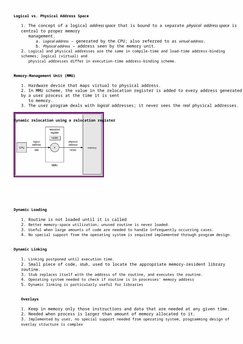
UNIT III-STORAGE MANAGEMENT
PART – A (2 MARKS)
1. Define logical address and physical address.
2. What is logical address space and physical address space?
3. What is the main function of the memory-management unit?
4. Define dynamic loading.
5. Define dynamic linking.
6. What are overlays?
7. Define swapping.
8. What are the common strategies to select a free hole from a set of available holes?
9. What do you mean by best fit?
10. What do you mean by first fit?
11. What is virtual memory?
12. What is Demand paging?
13. Define lazy swapper.
14. What is a pure demand paging?
15. Define effective access time.
16. Define secondary memory.
17. What is the basic approach of page replacement?
18. What are the various page replacement algorithms used for page replacement?
19. What are the major problems to implement demand paging?
20. What is a reference string?
21. Define virtual memory
PART-B
1. Explain about contiguous memory allocation. (16)
2. Give the basic concepts about paging. (16)

3. Write about the techniques for structuring the page table. (16)
4. Explain the basic concepts of segmentation. (16)
5. What is demand paging and what is its use? (16)
6. Explain the various page replacement strategies. (16)
7. What is thrashing and explain the methods to avoid thrashing? (16)
8. What is meant by virtual memory? Give some major benefits which are making
applicable. (16)
9. Consider the following page reference string.
1,2,7,8,3,4,2,1,4,2,5,6.How many page fault would occur for the following page
replacements algorithms, assuming an allocation of 3 frames?
(i)LRU
(i )FIFO
(i i)Optimal (16)
10. a)Explain about implementation details for file and directory. (8)
b)Given memory partitions of 100k,500k,200k,300k and 600k(in order)how would
each of the first fit, best fit and worst fit algorthim please process of 412k,317k,112k
and 326k(in order)? (8)

File system interface – File concept – Access methods – Directory structure – Filesystem mounting – Protection –
File system implementation – Directory implementation – Allocation methods – Free space management – Efficiency and performance – Recovery – Log-structured file systems – Case studies – File system in linux – File system inWindows XP.
UNIT-IV
File-System Interface
1. File Concept 2. Access Methods 3. Directory Structure 4. File System Mounting 5. File Sharing 6. Protection
File Concept
1. Contiguous logical address space 2. Types:
a. Data i. numeric ii. character iii. binary
b. Program
File Structure
1. None - sequence of words, bytes 2. Simple record structure
a. Lines b. Fixed length c. Variable length
3. Complex Structures a. Formatted document b. Relocatable load file
4. Can simulate last two with first method by inserting appropriate control characters. 5. Who decides:
a. Operating system b. Program
File Attributes
1. Name – only information kept in human-readable form. 2. Type – needed for systems that support different types. 3. Location – pointer to file location on device. 4. Size – current file size. 5. Protection – controls who can do reading, writing, executing. 6. Time, date, and user identification – data for protection, security, and usage monitoring. 7. Information about files are kept in the directory structure, which is maintained on the disk.

File Operations
1. Create 2. Write 3. Read 4. Reposition within file – file seek 5. Delete 6. Truncate 7. Open(Fi) – search the directory structure on disk for entry Fi, and move the content of entry to memory. 8. Close (Fi) – move the content of entry Fi in memory to directory structure on disk.
File Types – Name, Extension
Access Methods
1. Sequential Access read next
write next
reset
no read after last write
(rewrite)
2. Direct Access
read n
write n
position to n
read next
write next
rewrite n

n = relative block number
Sequential-access File
Simulation of Sequential Access on a Direct-access File
Example of Index and Relative Files
Directory Structure
A collection of nodes containing information about all files. Both the directory structure and the files reside on disk. Backups of these two structures are kept on tapes.
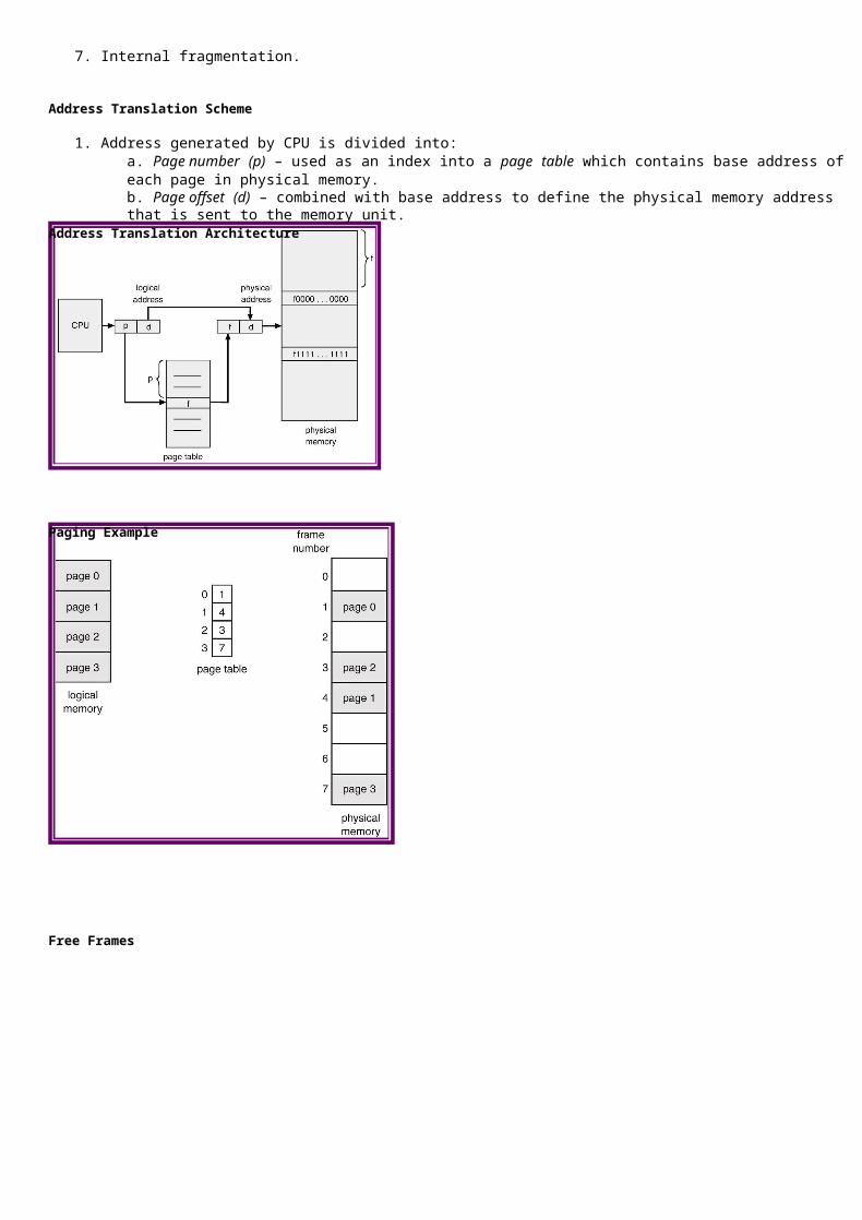
A Typical File-system Organization
Information in a Device Directory
1. Name 2. Type 3. Address 4. Current length 5. Maximum length 6. Date last accessed (for archival) 7. Date last updated (for dump) 8. Owner ID (who pays) 9. Protection information (discuss later)
Operations Performed on Directory
1. Search for a file 2. Create a file 3. Delete a file 4. List a directory 5. Rename a file 6. Traverse the file system
Organize the Directory (Logically) to Obtain
1. Efficiency – locating a file quickly. 2. Naming – convenient to users.
a. Two users can have same name for different files. b. The same file can have several different names.
3. Grouping – logical grouping of files by properties (e g all Hava programs all games )
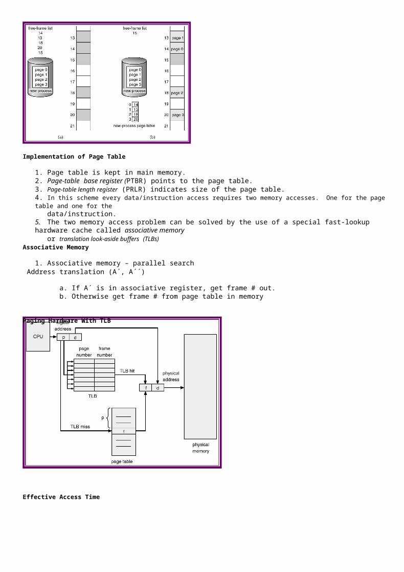
Single-Level Directory
A single directory for all users.
Two-Level Directory
Separate directory for each user.
• Path name • Can have the same file name for different user • Efficient searching • No grouping capability
Tree-Structured Directories
1. Efficient searching 2. Grouping Capability 3. Current directory (working directory)
a. cd /spell/mail/prog b. type list
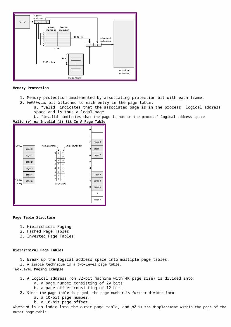
1. Absolute or relative path name 2. Creating a new file is done in current directory. 3. Delete a file
rm <file-name>
4. Creating a new subdirectory is done in current directory. mkdir <dir-name>
Example: if in current directory /mail
mkdir count
Deleting “mail” deleting the entire subtree rooted by “mail”
Acyclic-Graph Directories
Have shared subdirectories and files.
1. Two different names (aliasing) 2. If dict deletes list dangling pointer.
Solutions:
Backpointers, so we can delete all pointers. Variable size records a problem.
Backpointers using a daisy chain organization. Entry-hold-count solution.
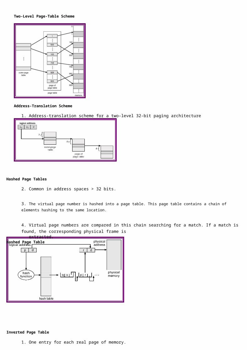
General Graph Directory
1. How do we guarantee no cycles? a. Allow only links to file not subdirectories. b. Garbage collection. c. Every time a new link is added use a cycle detection
algorithm to determine whether it is OK.
File System Mounting
1. A file system must be mounted before it can be accessed.
2. A unmounted file system (I.e. Fig. 11-11(b)) is mounted at a mount point.
(a) Existing. (b) Unmounted Partition
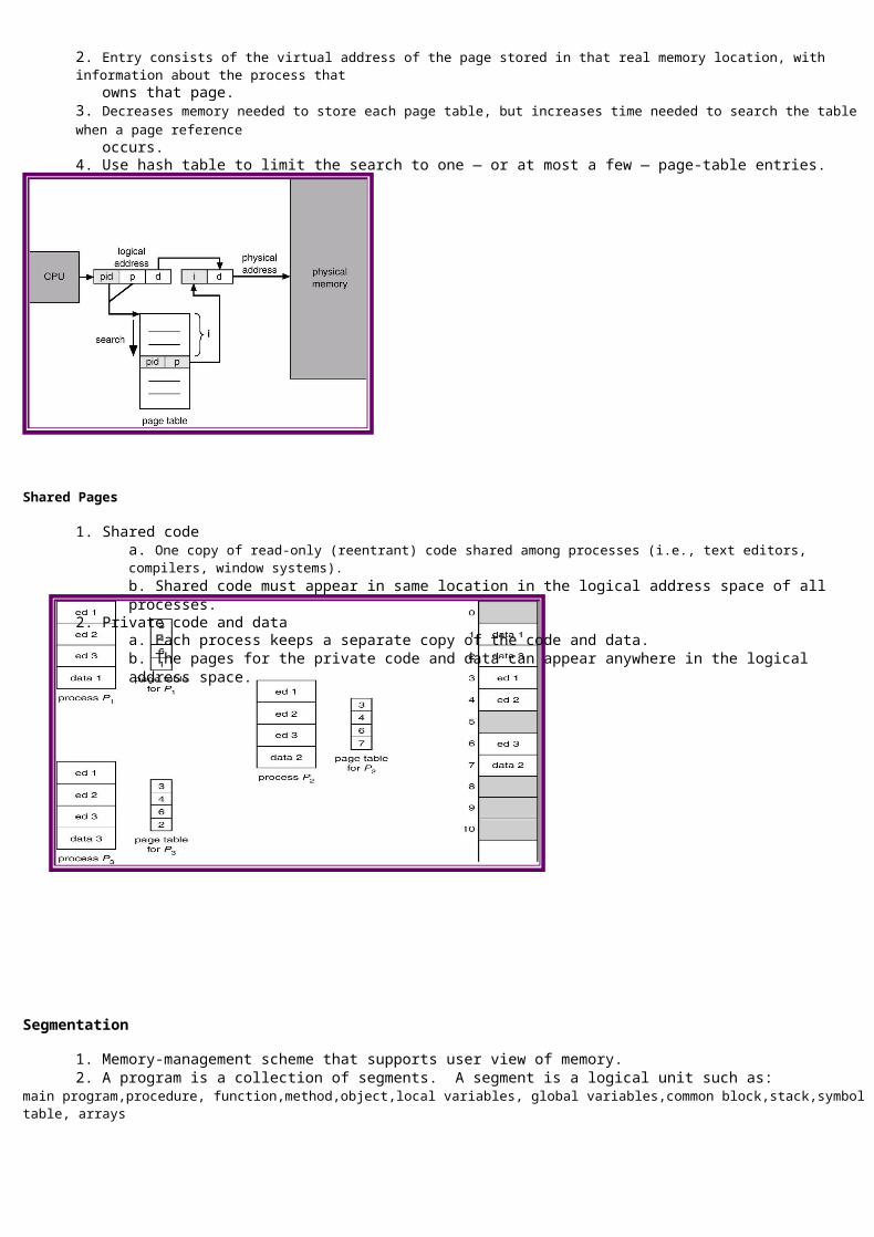
Mount Point
File Sharing
Sharing of files on multi-user systems is desirable. Sharing may be done through a protection scheme. On distributed systems, files may be shared across a network. Network File System (NFS) is a common distributed file-sharing method.
Protection
1. File owner/creator should be able to control: a. what can be done b. by whom
2. Types of access a. Read b. Write c. Execute d. Append e. Delete f. List
Access Lists and Groups
Mode of access: read, write, execute Three classes of users
RWX
a) owner access 71 1 1
RWX
b) group access 6 1 1 0
RWX
c) public access 10 0 1
Ask manager to create a group (unique name), say G, and add some users to the group. For a particular file (say game) or subdirectory, define an appropriate access.
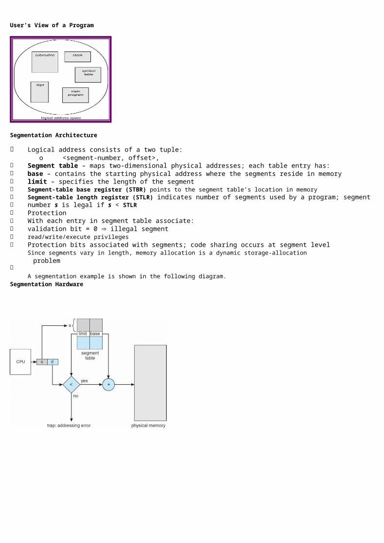
File System Implementation
1. File System Structure 2. File System Implementation 3. Directory Implementation 4. Allocation Methods 5. Free-Space Management 6. Efficiency and Performance 7. Recovery 8. Log-Structured File Systems 9. NFS
File-System Structure
1. File structure a. Logical storage unit b. Collection of related information
2. File system resides on secondary storage (disks). 3. File system organized into layers. 4. File control block – storage structure consisting of information about a file.
Layered File System
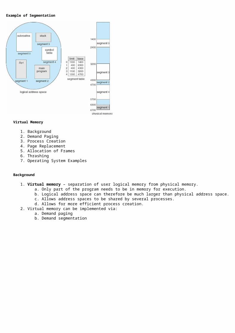
A Typical File Control Block
In-Memory File System Structures
1. The following figure illustrates the necessary file system structures provided by the operating systems. 2. Figure (a) refers to opening a file. 3. Figure (b) refers to reading a file.
Virtual File Systems
1. Virtual File Systems (VFS) provide an object-oriented way of implementing file systems. 2. VFS allows the same system call interface (the API) to be used for different types of file systems. 3. The API is to the VFS interface, rather than any specific type of file system.
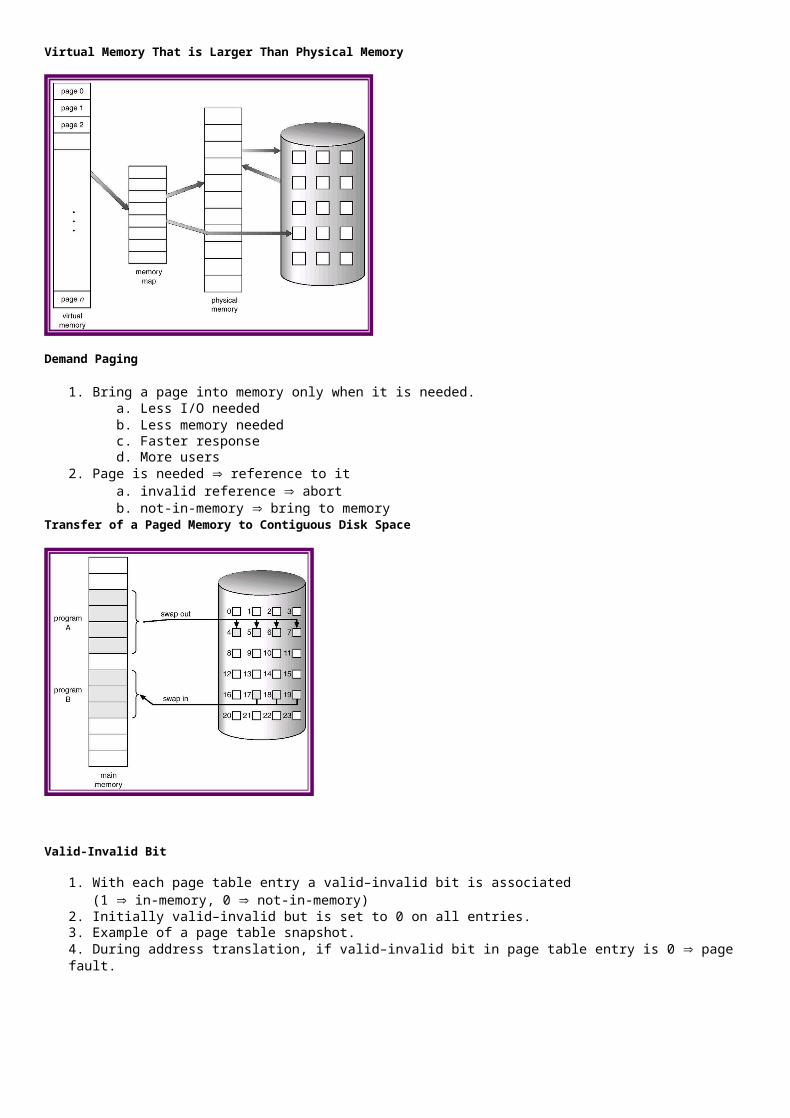
Directory Implementation
1. Linear list of file names with pointer to the data blocks. a. simple to program b. time-consuming to execute
2. Hash Table – linear list with hash data structure. a. decreases directory search time b. collisions – situations where two file names hash to the same location c. fixed size
Allocation Methods
i. An allocation method refers to how disk blocks are allocated for files: Contiguous allocation Linked allocation Indexed allocation
Contiguous Allocation
1. Each file occupies a set of contiguous blocks on the disk. 2. Simple – only starting location (block #) and length (number of blocks) are required. 3. Random access. 4. Wasteful of space (dynamic storage-allocation problem). 5. Files cannot grow.
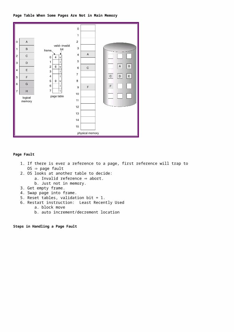
Contiguous Allocation of Disk Space
Extent-Based Systems
1. Many newer file systems (I.e. Veritas File System) use a modified contiguous allocation scheme. 2. Extent-based file systems allocate disk blocks in extents. 3. An extent is a contiguous block of disks. Extents are allocated for file allocation. A file consists of one or more extents.
Linked Allocation
1. Each file is a linked list of disk blocks: blocks may be scattered anywhere on the disk. 2. Simple – need only starting address 3. Free-space management system – no waste of space 4. No random access 5. Mapping
Block to be accessed is the Qth block in the linked chain of blocks representing the file.
Displacement into block = R + 1
File-allocation table (FAT) – disk-space allocation used by MS-DOS and OS/2.
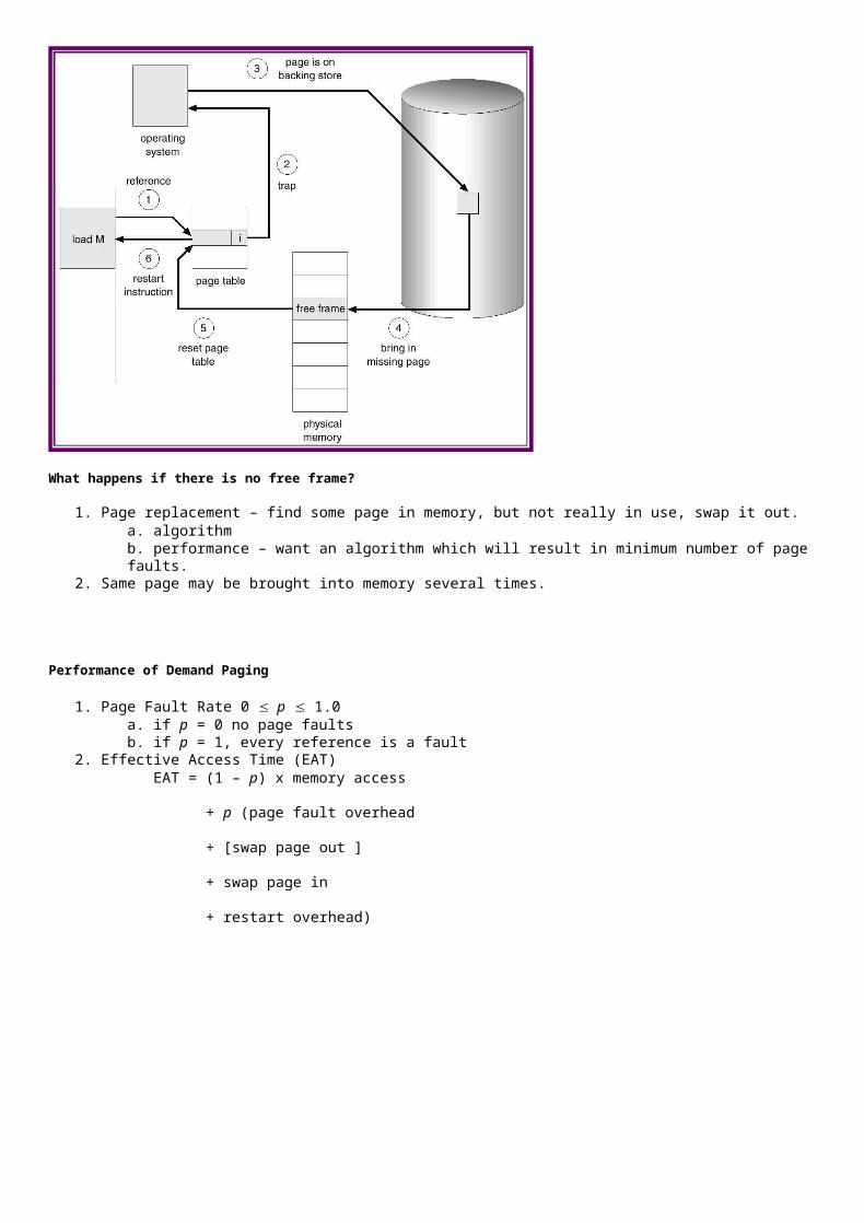
File-Allocation Table
Indexed Allocation
1. Brings all pointers together into the index block.2. Logical view.
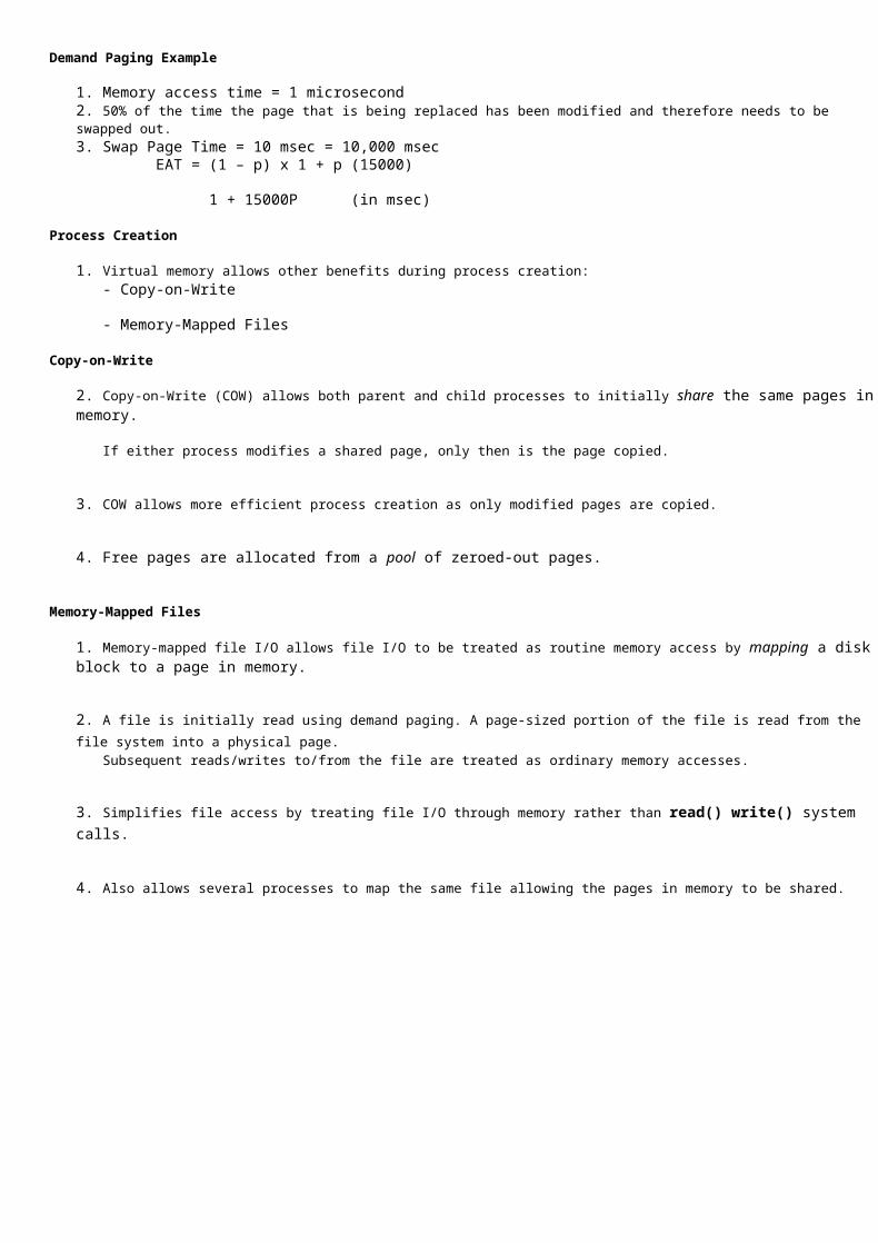
Need index table Random access Dynamic access without external fragmentation, but have overhead of index block. Mapping from logical to physical in a file of maximum size of 256K words and block size of 512 words. We need only 1 block for
index table.
Q = displacement into index table
R = displacement into block
1. Mapping from logical to physical in a file of unbounded length (block size of 512 words). 2. Linked scheme – Link blocks of index table (no limit on size).
3. Mapping from logical to physical in a file of unbounded length (block size of 512 words). 4. Linked scheme – Link blocks of index table (no limit on size).
5. -level index (maximum file size is 5123)
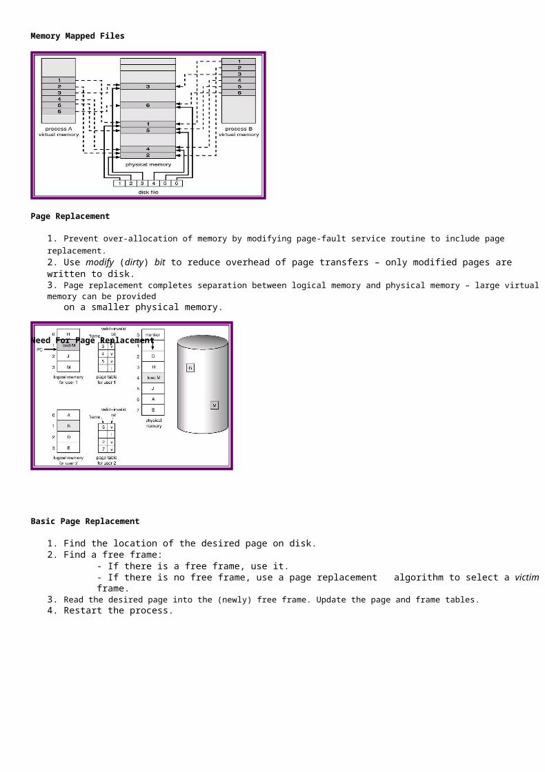
Combined Scheme: UNIX (4K bytes per block)
Free-Space Management
Block number calculation
(number of bits per word) *
(number of 0-value words) +
offset of first 1 bit
Bit map requires extra space. Example: block size = 212 bytes
disk size = 230 bytes (1 gigabyte)
n = 230/212 = 218 bits (or 32K bytes)
1. Easy to get contiguous files
2. Linked list (free list)
a. Cannot get contiguous space easily
b. No waste of space 3. Grouping
4. Counting
5.Need to protect:
o Pointer to free list o Bit map
Must be kept on disk Copy in memory and disk may differ. Cannot allow for block[i] to have a situation where bit[i] = 1 in memory and bit[i] = 0 on disk.
o Solution: Set bit[i] = 1 in disk. Allocate block[i] Set bit[i] = 1 in memory
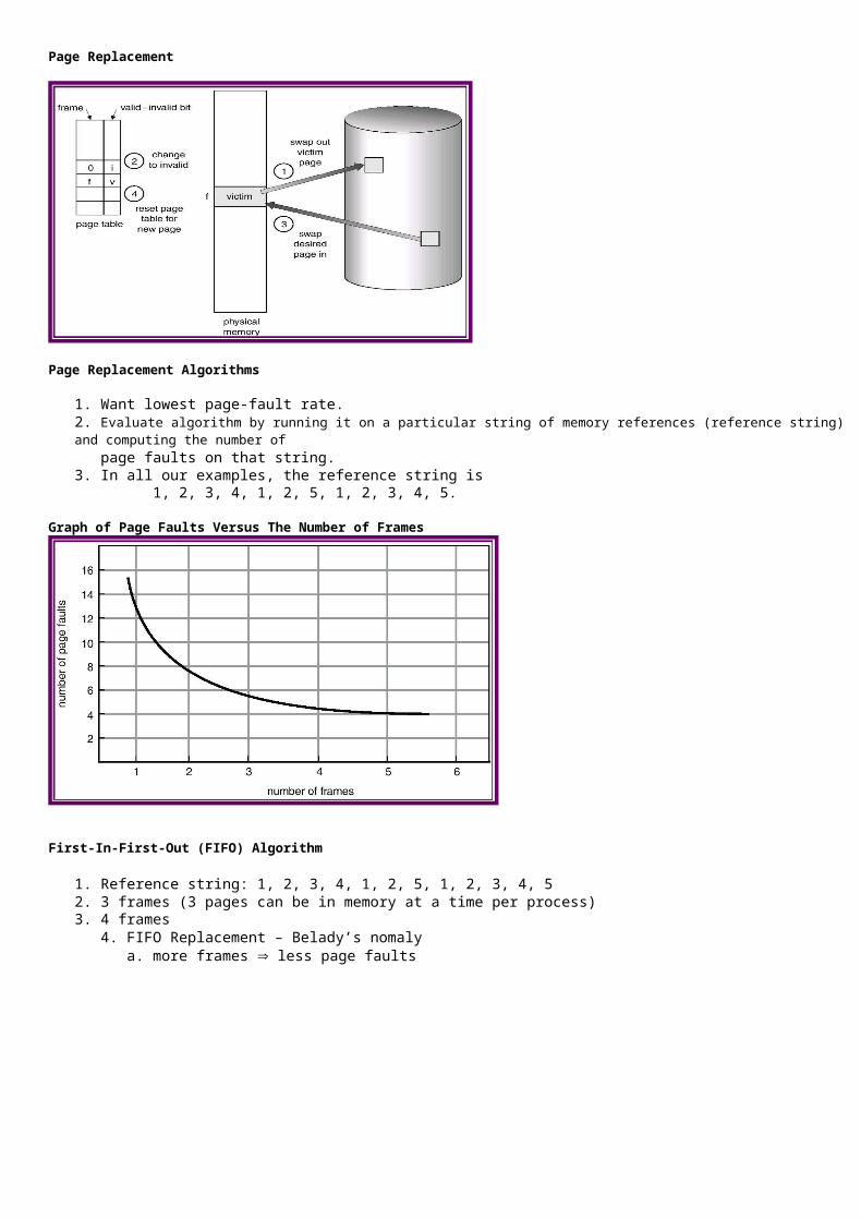
Linked Free Space List on Disk
Efficiency and Performance
1. Efficiency dependent on: a. disk allocation and directory algorithms b. types of data kept in file’s directory entry
2. Performance a. disk cache – separate section of main memory for frequently used blocks b. free-behind and read-ahead – techniques to optimize sequential access c. improve PC performance by dedicating section of memory as virtual disk, or RAM disk.
Various Disk-Caching Locations
Page Cache
1. A page cache caches pages rather than disk blocks using virtual memory techniques. 2. Memory-mapped I/O uses a page cache. 3. Routine I/O through the file system uses the buffer (disk) cache. 4. This leads to the following figure.
I/O Without a Unified Buffer Cache
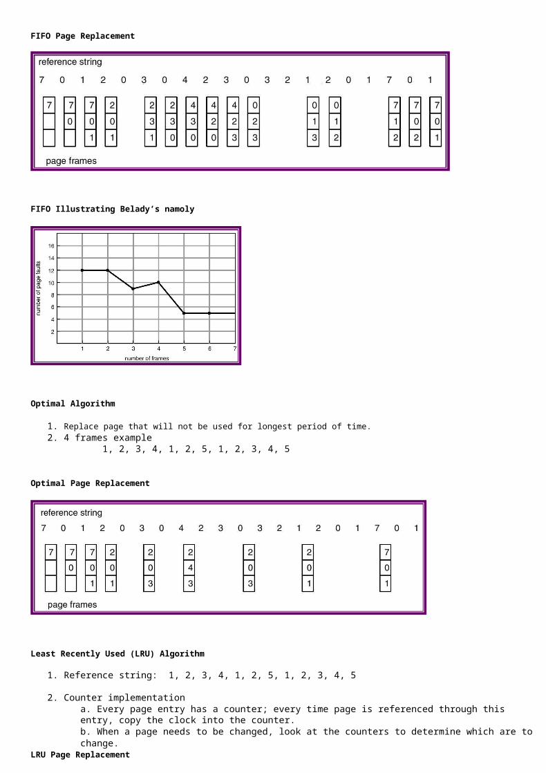
Unified Buffer Cache
1. A unified buffer cache uses the same page cache to cache both memory-mapped pages and ordinary file system I/O.
I/O Using a Unified Buffer Cache
Recovery
1. Consistency checking – compares data in directory structure with data blocks on disk, and tries to fix inconsistencies. 2. Use system programs to back up data from disk to another storage device (floppy disk, magnetic tape). 3. Recover lost file or disk by restoring data from backup.
Log Structured File Systems
1. Log structured (or journaling) file systems record each update to the file system as a transaction. 2. All transactions are written to a log. A transaction is considered committed once it is written to the log. However, the file
system may not yet be updated. 3. The transactions in the log are asynchronously written to the file system. When the file system is modified, the transaction is
removed from the log. 4. If the file system crashes, all remaining transactions in the log must still be performed.
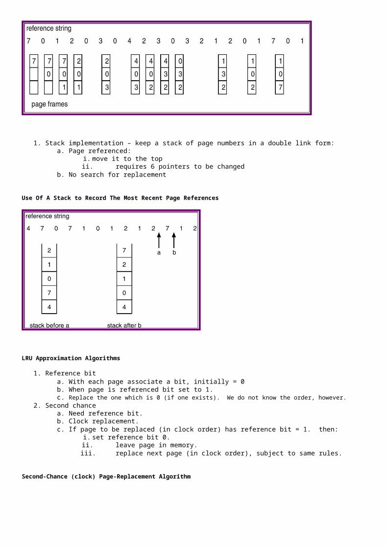
UNIT IV- FILE SYSTEMS
PART – A (2 MARKS)
1. What is a file?
2. List the various file attributes.
3. What are the various file operations?
4. What are the information associated with an open file?
5. What are the different accessing methods of a file?
6. What is Directory?
7. What are the operations that can be performed on a directory?
8. What are the most common schemes for defining the logical structure of a directory?
9. Define UFD and MFD.
10. What is a path name?
11. What are the various layers of a file system?
12. What are the structures used in file-system implementation?
13. What are the functions of virtual file system (VFS)?
14. Why is the production needed in file sharing system?
15. List the features of Linux system
16. Briefly discuss the relative advantages and disadvantages of sector sparing and sector slipping
17. What is meant by OS platform independent?
18. Write about windows2000 file protection and security services.
19. Define LDAP
PART-B
1. What are files and explain the access methods for files? (16)
2. Explain the schemes for defining the logical structure of a directory. (16)
3. Write notes about the protection strategies provided for files. (16)
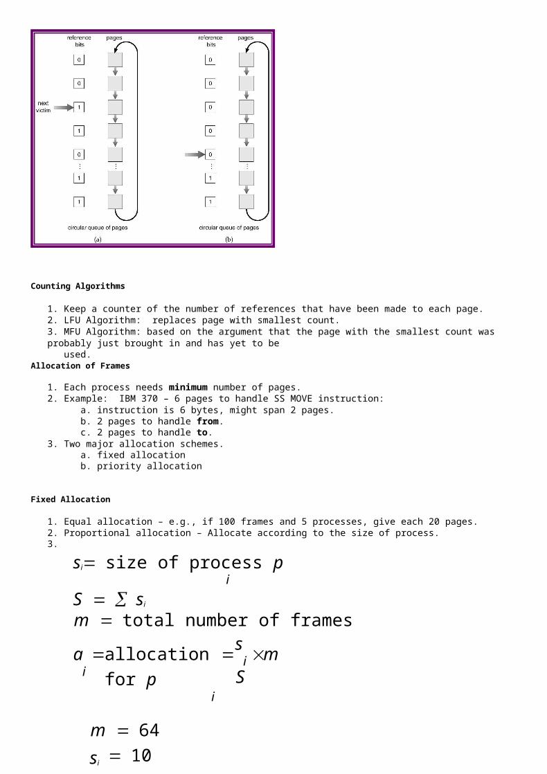
4. What are the file allocation methods and explain it (16)
5. Explain about the free space management (16)
6. Explain the schemes for defining the logical structure of a directory. (16)

UNIT V I/O SYSTEMS
I/O systems – I/O hardware – Application I/O interface – Kernel I/O subsystem – Streams – Performance – Mass-storage structure – Disk scheduling – Disk management – Swap-space management – RAID – Disk attachment – Stable storage – Tertiary storage – Case study – I/O in linux.
UNIT -V
I/O Systems
1. I/O Hardware 2. Application I/O Interface 3. Kernel I/O Subsystem 4. Transforming I/O Requests to Hardware Operations 5. Streams 6. Performance
I/O Hardware
Incredible variety of I/O devices Common concepts Port Bus (daisy chain or shared direct access) Controller (host adapter) I/O instructions control devices Devices have addresses, used by Direct I/O instructions Memory-mapped I/O
A Typical PC Bus Structure
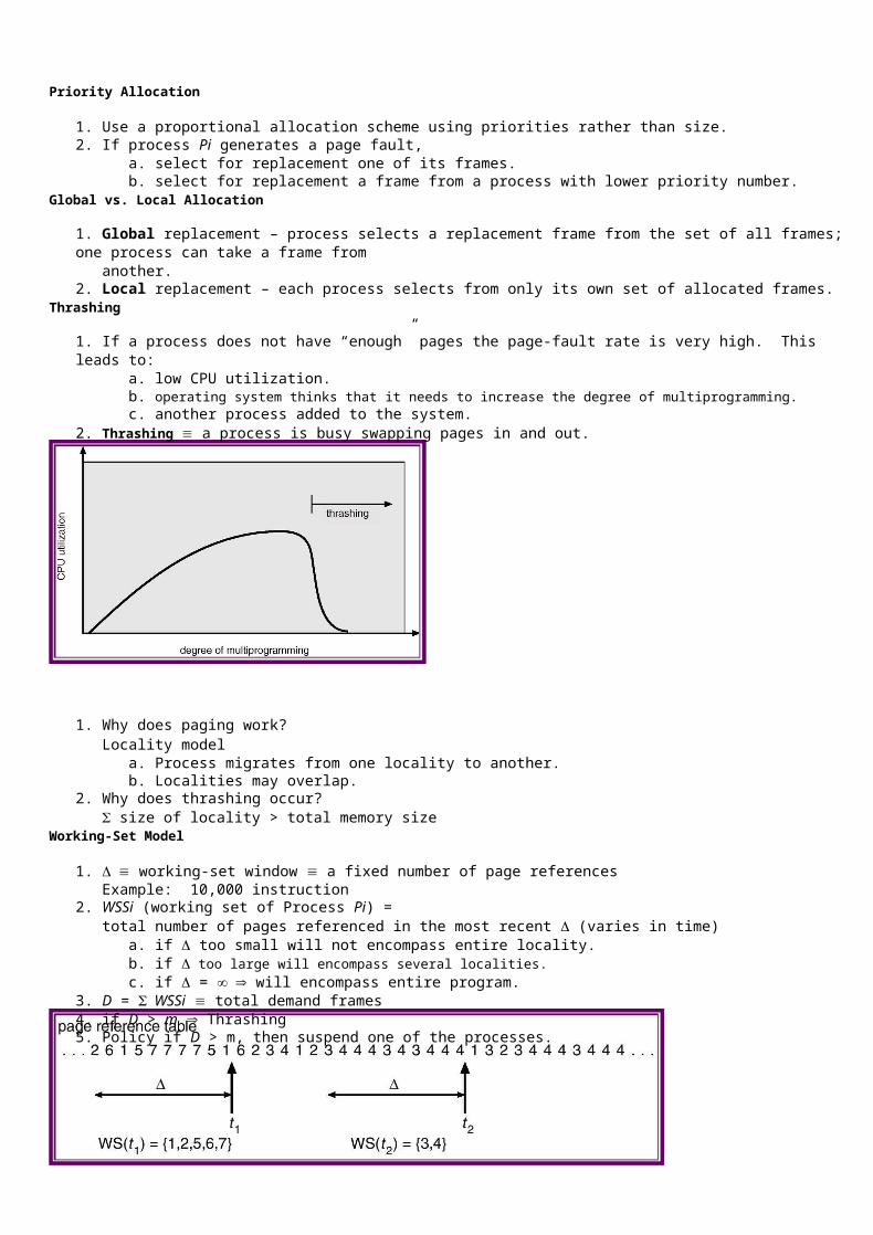
Device I/O Port Locations on PCs (partial)
Polling
Determines state of device command-ready busy Error Busy-wait cycle to wait for I/O from device
Interrupts
CPU Interrupt request line triggered by I/O device Interrupt handler receives interrupts Maskable to ignore or delay some interrupts Interrupt vector to dispatch interrupt to correct handler Based on priority Some unmaskable Interrupt mechanism also used for exceptions Interrupt-Driven I/O Cycle

Intel Pentium Processor Event-Vector Table
Direct Memory Access
Used to avoid programmed I/O for large data movement Requires DMA controller Bypasses CPU to transfer data directly between I/O device and memory
Six Step Process to Perform DMA Transfer
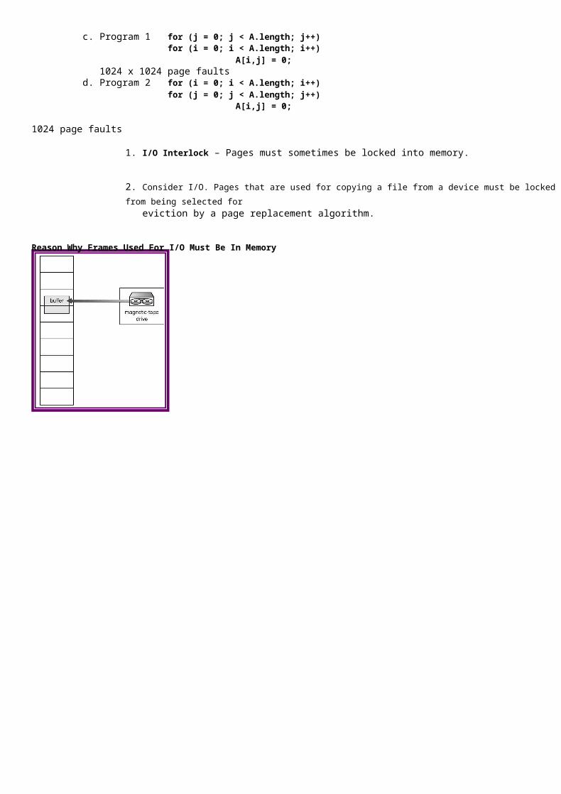
Application I/O Interface
I/O system calls encapsulate device behaviors in generic classes
Device-driver layer hides differences among I/O controllers from kernel
Devices vary in many dimensions
Character-stream or block Sequential or random-access Sharable or dedicated Speed of operation read-write, read only, or write only
A Kernel I/O Structure
Characteristics of I/O Devices
Block and Character Devices
Block devices include disk drives Commands include read, write, seek Raw I/O or file-system access Memory-mapped file access possible Character devices include keyboards, mice, serial ports Commands include get, put Libraries layered on top allow line editing
Network Devices
Varying enough from block and character to have own interface Unix and Windows NT/9i/2000 include socket interface Separates network protocol from network operation Includes select functionality Approaches vary widely (pipes, FIFOs, streams, queues, mailboxes)
Clocks and Timers
Provide current time, elapsed time, timer If programmable interval time used for timings, periodic interrupts
ioctl (on UNIX) covers odd aspects of I/O such as clocks and timers
Blocking and Nonblocking I/O
Blocking - process suspended until I/O completed Easy to use and understand Insufficient for some needs
Nonblocking - I/O call returns as much as available User interface, data copy (buffered I/O) Implemented via multi-threading Returns quickly with count of bytes read or written Asynchronous - process runs while I/O executes Difficult to use
I/O subsystem signals process when I/O completed
Kernel I/O Subsystem
Scheduling Some I/O request ordering via per-device queue Some OSs try fairness Buffering - store data in memory while transferring between devices To cope with device speed mismatch To cope with device transfer size mismatch To maintain “copy semantics” Caching - fast memory holding copy of data Always just a copy Key to performance Spooling - hold output for a device If device can serve only one request at a time i.e., Printing Device reservation - provides exclusive access to a device System calls for allocation and deallocation Watch out for deadlock
Error Handling
OS can recover from disk read, device unavailable, transient write failures Most return an error number or code when I/O request fails System error logs hold problem reports
Kernel Data Structures
Kernel keeps state info for I/O components, including open file tables, network connections, character device state Many many complex data structures to track buffers memory allocation “dirty” blocks Some use object-oriented methods and message passing to implement I/O
UNIX I/O Kernel Structure
I/O Requests to Hardware Operations
Consider reading a file from disk for a process: Determine device holding file Translate name to device representation Physically read data from disk into buffer Make data available to requesting process Return control to process
Life Cycle of An I/O Request
STREAMS
STREAM – a full-duplex communication channel between a user-level process and a device A STREAM consists of:
- STREAM head interfaces with the user process
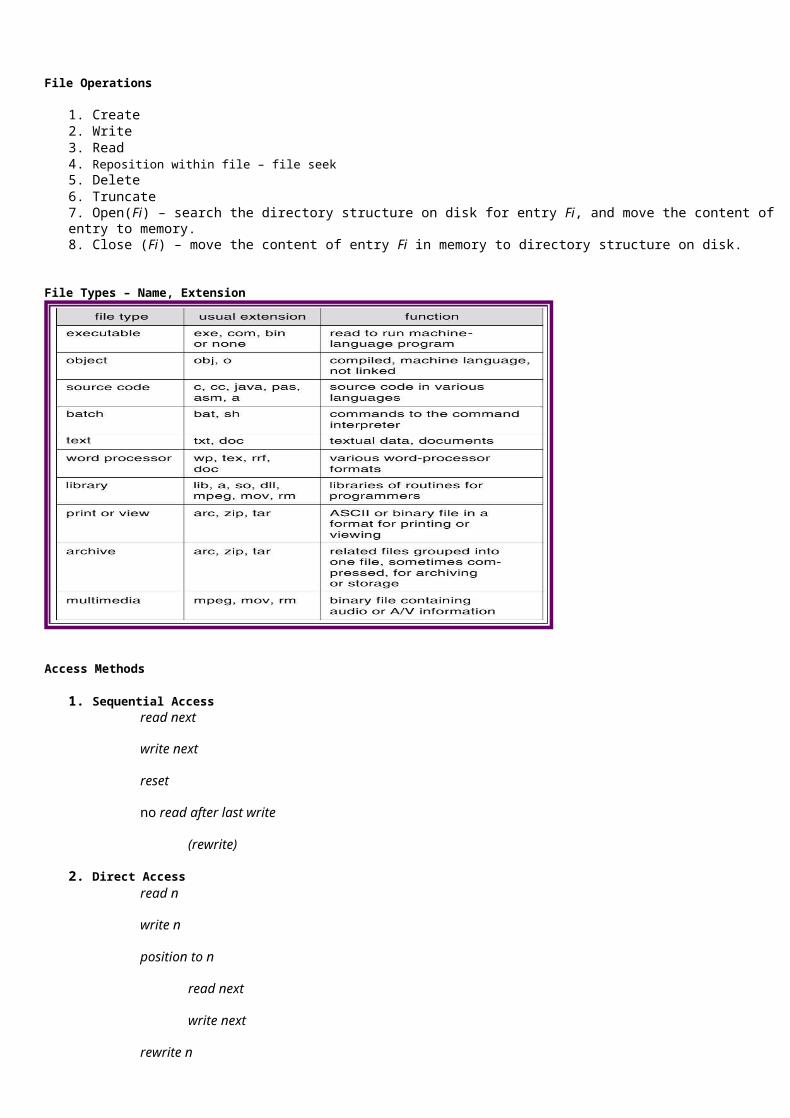
- driver end interfaces with the device - zero or more STREAM modules between them.
Each module contains a read queue and a write queue Message passing is used to communicate between queues
The STREAMS Structure
Performance
I/O a major factor in system performance: Demands CPU to execute device driver, kernel I/O code Context switches due to interrupts Data copying Network traffic especially stressful
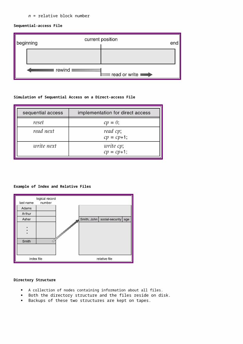
Intercomputer Communications
Improving Performance
Reduce number of context switches Reduce data copying Reduce interrupts by using large transfers, smart controllers, polling Use DMA Balance CPU, memory, bus, and I/O performance for highest throughput
Device-Functionality Progression
Mass-Storage Systems
1. Disk Structure

2. Disk Scheduling 3. Disk Management 4. Swap-Space Management 5. RAID Structure 6. Disk Attachment 7. Stable-Storage Implementation 8. Tertiary Storage Devices
Disk Structure
1. Disk drives are addressed as large 1-dimensional arrays of logical blocks, where the logical block is the smallest unit of transfer. 2. The 1-dimensional array of logical blocks is mapped into the sectors of the disk sequentially.
a. Sector 0 is the first sector of the first track on the outermost cylinder. b. Mapping proceeds in order through that track, then the rest of the tracks in that cylinder, and then through the rest of
the cylinders from outermost to innermost. Disk Scheduling
1. The operating system is responsible for using hardware efficiently — for the disk drives, this means having a fast access time and disk bandwidth.
2. Access time has two major components a. Seek time is the time for the disk are to move the heads to the cylinder containing the desired sector. b. Rotational latency is the additional time waiting for the disk to rotate the desired sector to the disk head.
3. Minimize seek time 4. Seek time seek distance 5. Disk bandwidth is the total number of bytes transferred, divided by the total time between the first request for service and the
completion of the last transfer. 6. Several algorithms exist to schedule the servicing of disk I/O requests. 7. We illustrate them with a request queue (0-199).
98, 183, 37, 122, 14, 124, 65, 67
Head pointer 53
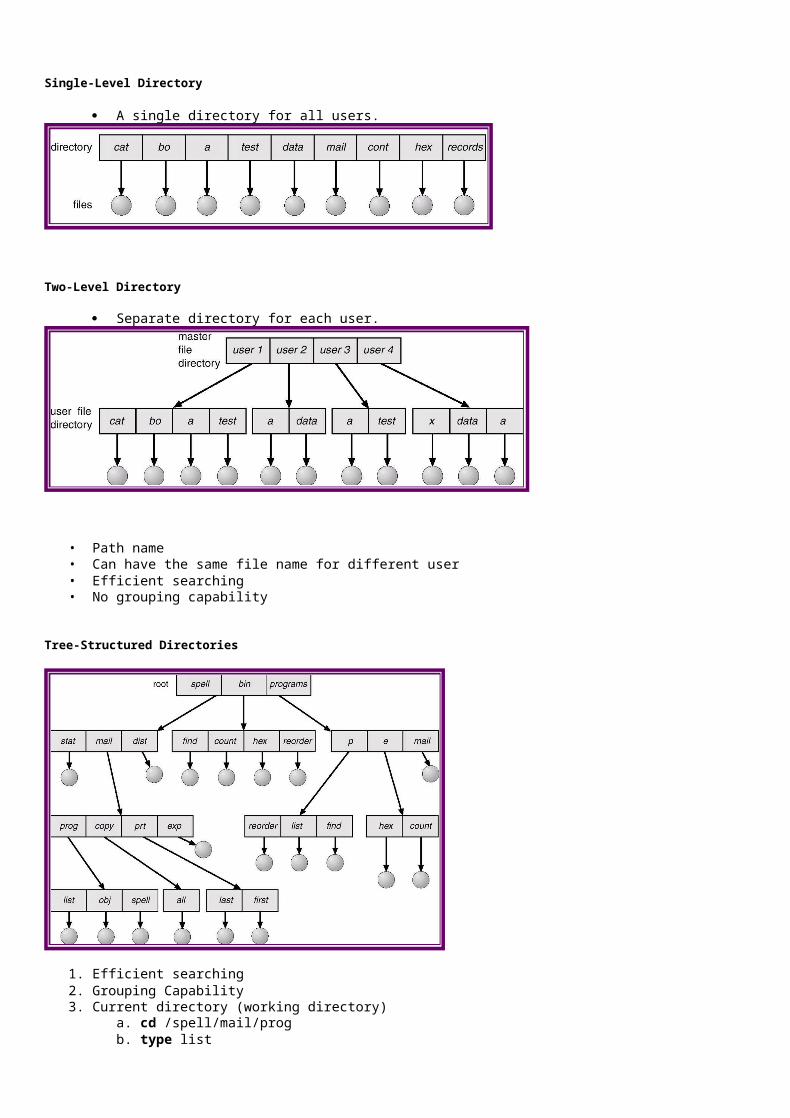
FCFS
Illustration shows total head movement of 640 cylinders.
SSTF
1. Selects the request with the minimum seek time from the current head position. 2. SSTF scheduling is a form of SJF scheduling; may cause starvation of some requests. 3. Illustration shows total head movement of 236 cylinders.

SCAN
1. The disk arm starts at one end of the disk, and moves toward the other end, servicing requests until it gets to the other end of the disk, where the head movement is reversed and servicing continues.
2. Sometimes called the elevator algorithm. 3. Illustration shows total head movement of 208 cylinders.
C-SCAN
1. Provides a more uniform wait time than SCAN. 2. The head moves from one end of the disk to the other. servicing requests as it goes. When it reaches the other end, however,
it immediately returns to the beginning of the disk, without servicing any requests on the return trip. 3. Treats the cylinders as a circular list that wraps around from the last cylinder to the first one.
C-LOOK
1. Version of C-SCAN 2. Arm only goes as far as the last request in each direction, then reverses direction immediately, without first going all the way to
the end of the disk.
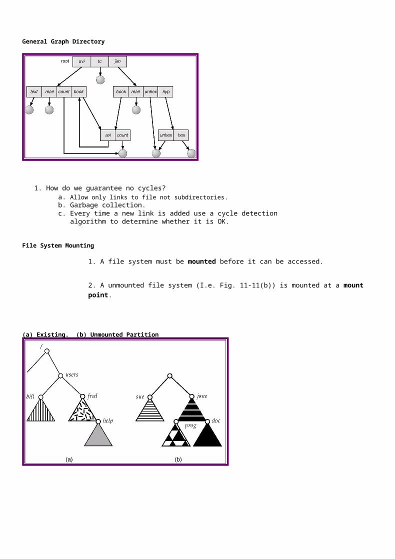
Selecting a Disk-Scheduling Algorithm
1. SSTF is common and has a natural appeal 2. SCAN and C-SCAN perform better for systems that place a heavy load on the disk. 3. Performance depends on the number and types of requests. 4. Requests for disk service can be influenced by the file-allocation method. 5. The disk-scheduling algorithm should be written as a separate module of the operating system, allowing it to be replaced with
a different algorithm if necessary. 6. Either SSTF or LOOK is a reasonable choice for the default algorithm.
Disk Management
1. Low-level formatting, or physical formatting — Dividing a disk into sectors that the disk controller can read and write. 2. To use a disk to hold files, the operating system still needs to record its own data structures on the disk.
a. Partition the disk into one or more groups of cylinders. b. Logical formatting or “making a file system”
3. Boot block initializes system. a. The bootstrap is stored in ROM. b. Bootstrap loader program.
4. Methods such as sector sparing used to handle bad blocks.
MS-DOS Disk Layout
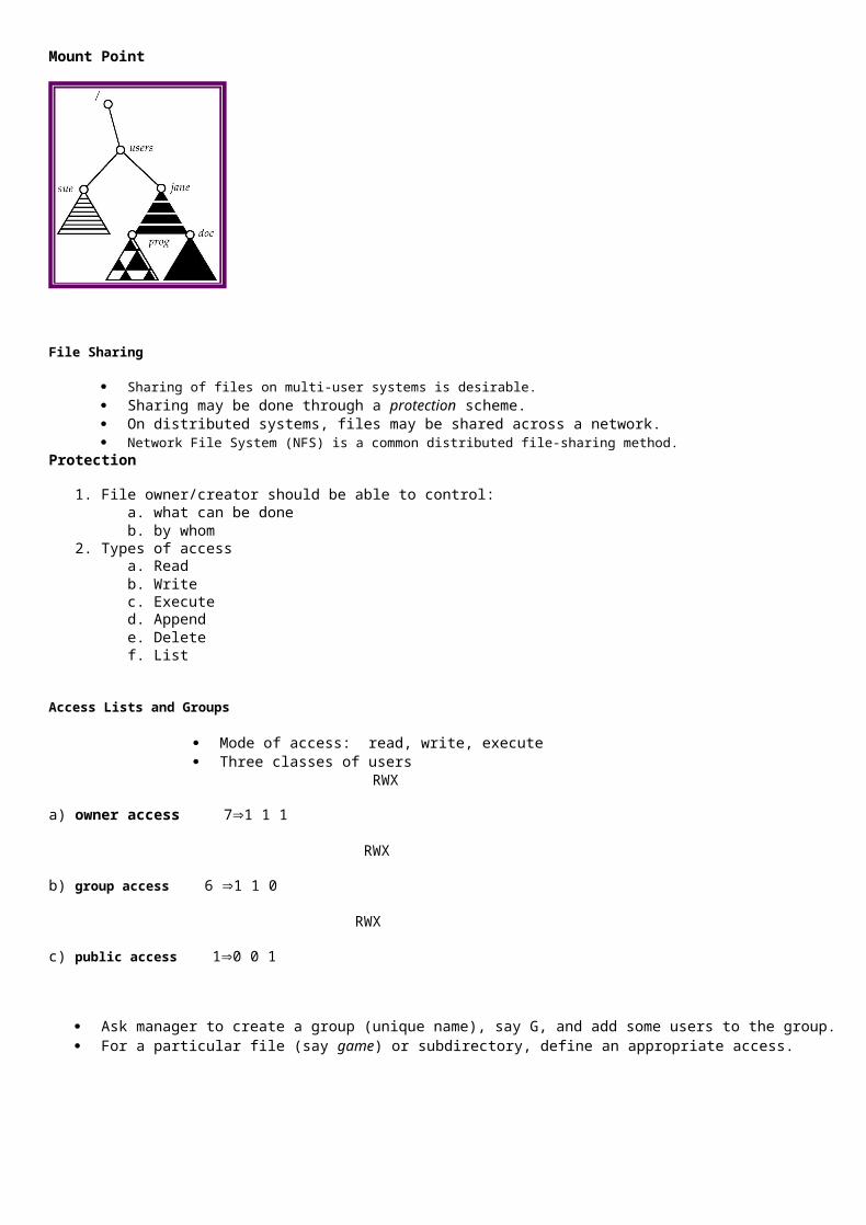
Swap-Space Management
1. Swap-space — Virtual memory uses disk space as an extension of main memory. 2. Swap-space can be carved out of the normal file system,or, more commonly, it can be in a separate disk partition. 3. Swap-space management
a. 4.3BSD allocates swap space when process starts; holds text segment (the program) and data segment. b. Kernel uses swap maps to track swap-space use. c. Solaris 2 allocates swap space only when a page is forced out of physical memory, not when the virtual memory page
is first created.
4.3 BSD Text-Segment Swap Map
4.3 BSD Data-Segment Swap Map
RAID Structure
1. RAID – multiple disk drives provides reliability via redundancy. 2. RAID is arranged into six different levels.
1. Several improvements in disk-use techniques involve the use of multiple disks working cooperatively. 2. Disk striping uses a group of disks as one storage unit. 3. RAID schemes improve performance and improve the reliability of the storage system by storing redundant data.
a. Mirroring or shadowing keeps duplicate of each disk. b. Block interleaved parity uses much less redundancy.
RAID Levels
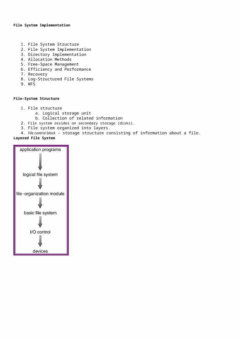
RAID (0 + 1) and (1 + 0)
Disk Attachment
Disks may be attached one of two ways:
Host attached via an I/O port
Network attached via a network connection
Network-Attached Storage
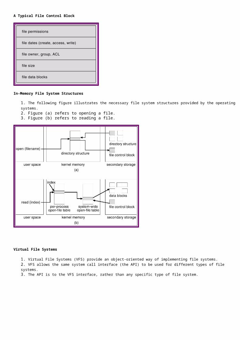
Storage-Area Network
Stable-Storage Implementation
1. Write-ahead log scheme requires stable storage. 2. To implement stable storage:
a. Replicate information on more than one nonvolatile storage media with independent failure modes. b. Update information in a controlled manner to ensure that we can recover the stable data after any failure during data
transfer or recovery.
Tertiary Storage Devices
1. Low cost is the defining characteristic of tertiary storage. 2. Generally, tertiary storage is built using removable media3. Common examples of removable media are floppy disks and CD-ROMs; other types are available.
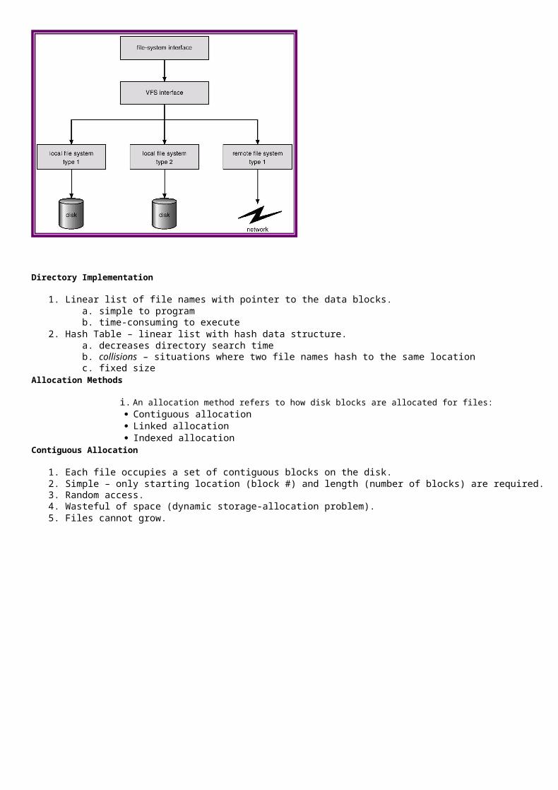
Removable Disks
1. Floppy disk — thin flexible disk coated with magnetic material, enclosed in a protective plastic case. a. Most floppies hold about 1 MB; similar technology is used for removable disks that hold more than 1 GB. b. Removable magnetic disks can be nearly as fast as hard disks, but they are at a greater risk of damage from exposure.
2. A magneto-optic disk records data on a rigid platter coated with magnetic material. a. Laser heat is used to amplify a large, weak magnetic field to record a bit. b. Laser light is also used to read data (Kerr effect). c. The magneto-optic head flies much farther from the disk surface than a magnetic disk head, and the magnetic
material is covered with a protective layer of plastic or glass; resistant to head crashes. 3. Optical disks do not use magnetism; they employ special materials that are altered by laser light.
WORM Disks
1. The data on read-write disks can be modified over and over. 2. WORM (“Write Once Read Many Times”) disks can be written only once 3. Thin aluminum film sandwiched between two glass or plastic platters. 4. To write a bit, the drive uses a laser light to burn a small hole through the aluminum; information can be destroyed by not
altered. 5. Very durable and reliable. 6. Read Only disks, such ad CD-ROM and DVD, com from the factory with the data pre-recorded.
Tapes
1. Compared to a disk, a tape is less expensive and holds more data, but random access is much slower. 2. Tape is an economical medium for purposes that do not require fast random access, e.g., backup copies of disk data, holding
huge volumes of data. 3. Large tape installations typically use robotic tape changers that move tapes between tape drives and storage slots in a tape
library. a. stacker – library that holds a few tapes b. silo – library that holds thousands of tapes
4. A disk-resident file can be archived to tape for low cost storage; the computer can stage it back into disk storage for active use.
Operating System Issues
1. Major OS jobs are to manage physical devices and to present a virtual machine abstraction to applications 2. For hard disks, the OS provides two abstraction:
a. Raw device – an array of data blocks. b. File system – the OS queues and schedules the interleaved requests from several applications.
Application Interface
1. Most OSs handle removable disks almost exactly like fixed disks — a new cartridge is formatted and an empty file system is generated on the disk.
2. Tapes are presented as a raw storage medium, i.e., and application does not not open a file on the tape, it opens the whole tape drive as a raw device.
3. Usually the tape drive is reserved for the exclusive use of that application. 4. Since the OS does not provide file system services, the application must decide how to use the array of blocks. 5. Since every application makes up its own rules for how to organize a tape, a tape full of data can generally only be used by the
program that created it. Tape Drives
1. The basic operations for a tape drive differ from those of a disk drive. 2. locate positions the tape to a specific logical block, not an entire track (corresponds to seek). 3. The read position operation returns the logical block number where the tape head is. 4. The space operation enables relative motion.
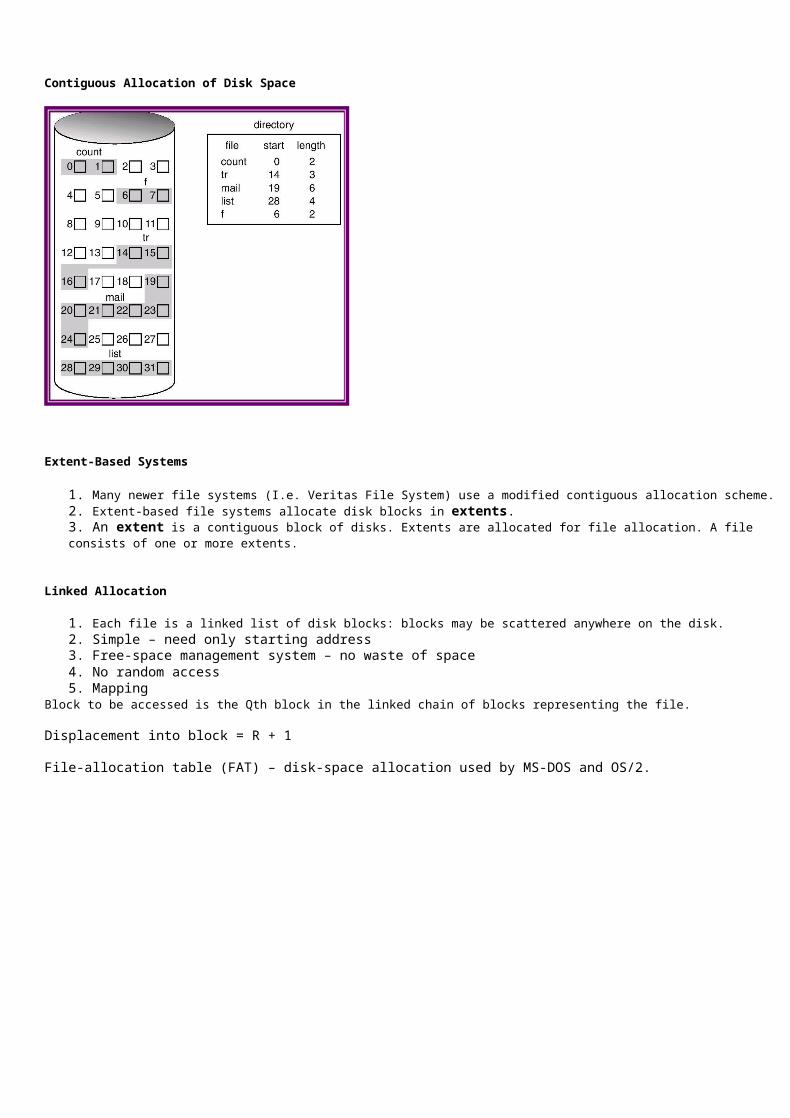
5. Tape drives are “append-only” devices updating a block in the middle of the tape also effectively erases everything beyondthat block.
6. An EOT mark is placed after a block that is written. File Naming
1. The issue of naming files on removable media is especially difficult when we want to write data on a removable cartridge on one computer, and then use the cartridge in another computer.
2. Contemporary OSs generally leave the name space problem unsolved for removable media, and depend on applications and users to figure out how to access and interpret the data.
3. Some kinds of removable media (e.g., CDs) are so well standardized that all computers use them the same way. Hierarchical Storage Management (HSM)
1. A hierarchical storage system extends the storage hierarchy beyond primary memory and secondary storage to incorporatetertiary storage — usually implemented as a jukebox of tapes or removable disks.
2. Usually incorporate tertiary storage by extending the file system. a. Small and frequently used files remain on disk. b. Large, old, inactive files are archived to the jukebox.
3. HSM is usually found in supercomputing centers and other large installations that have enormous volumes of data. Speed
1. Two aspects of speed in tertiary storage are bandwidth and latency. 2. Bandwidth is measured in bytes per second.
a. Sustained bandwidth – average data rate during a large transfer; # of bytes/transfer time. Data rate when the data stream is actually flowing.
b. Effective bandwidth – average over the entire I/O time, including seek or locate, and cartridge switching. Drive’s overall data rate
3. Access latency – amount of time needed to locate data. a. Access time for a disk – move the arm to the selected cylinder and wait for the rotational latency; < 35 milliseconds. b. Access on tape requires winding the tape reels until the selected block reaches the tape head; tens or hundreds of
seconds. c. Generally say that random access within a tape cartridge is about a thousand times slower than random access on
disk. 4. The low cost of tertiary storage is a result of having many cheap cartridges share a few expensive drives. 5. A removable library is best devoted to the storage of infrequently used data, because the library can only satisfy a relatively
small number of I/O requests per hour. Reliability
1. A fixed disk drive is likely to be more reliable than a removable disk or tape drive. 2. An optical cartridge is likely to be more reliable than a magnetic disk or tape. 3. A head crash in a fixed hard disk generally destroys the data, whereas the failure of a tape drive or optical disk drive often
leaves the data cartridge unharmed.
Cost
1. Main memory is much more expensive than disk storage 2. The cost per megabyte of hard disk storage is competitive with magnetic tape if only one tape is used per drive. 3. The cheapest tape drives and the cheapest disk drives have had about the same storage capacity over the years. 4. Tertiary storage gives a cost savings only when the number of cartridges is considerably larger than the number of drives.
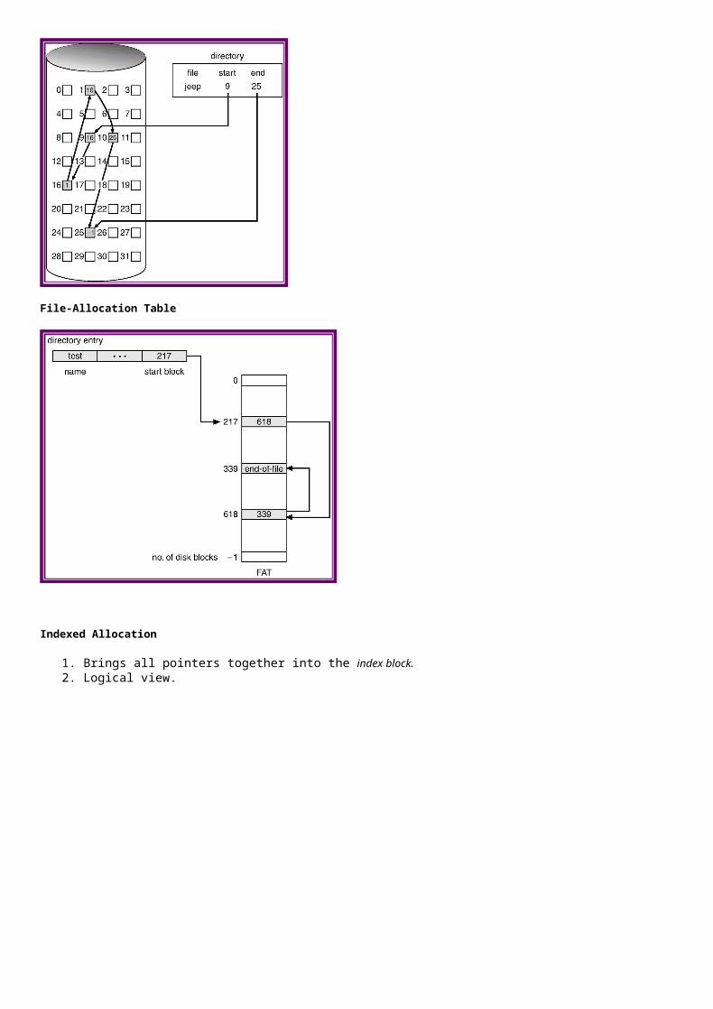
UNIT – V -I/O SYSTEMS
PART – A (2 MARKS)
1. Define seek time and latency time.
2. What are the allocation methods of a disk space?
3. What are the advantages of Contiguous allocation?
4. What are the drawbacks of contiguous allocation of disk space?
5. What are the advantages of Linked allocation?
6. What are the disadvantages of linked allocation?
7. What are the advantages of Indexed allocation?
8. How can the index blocks be implemented in the indexed allocation scheme?
9. Define rotational latency and disk bandwidth.
10. How free-space is managed using bit vector implementation?
11. Define buffering.
12. Define caching.
13. Define spooling.
14. What are the various disk-scheduling algorithms?
15. What is low-level formatting?
16. What is the use of boot block?
17. What is sector sparing?
PART-B
1. Write about the kernel I/O subsystem. (16)
2. Explain the various disk scheduling techniques (16)
3. Write notes about disk management and swap-space management. (16)
4. What is mean by RAID and explain it in detail (16)
5. Discuss about stable and tertiary storages (16)
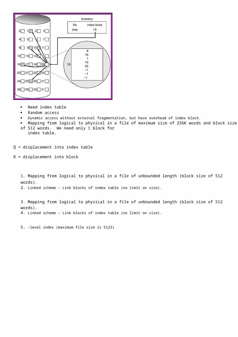
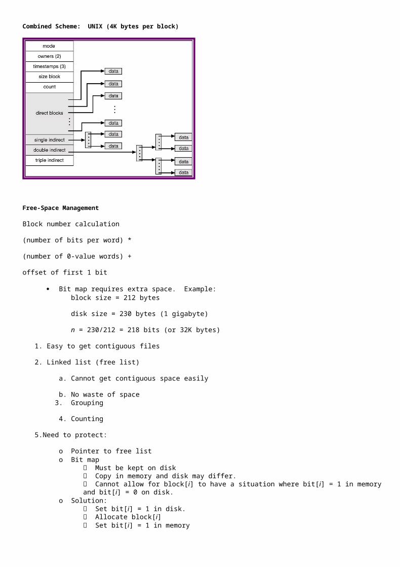
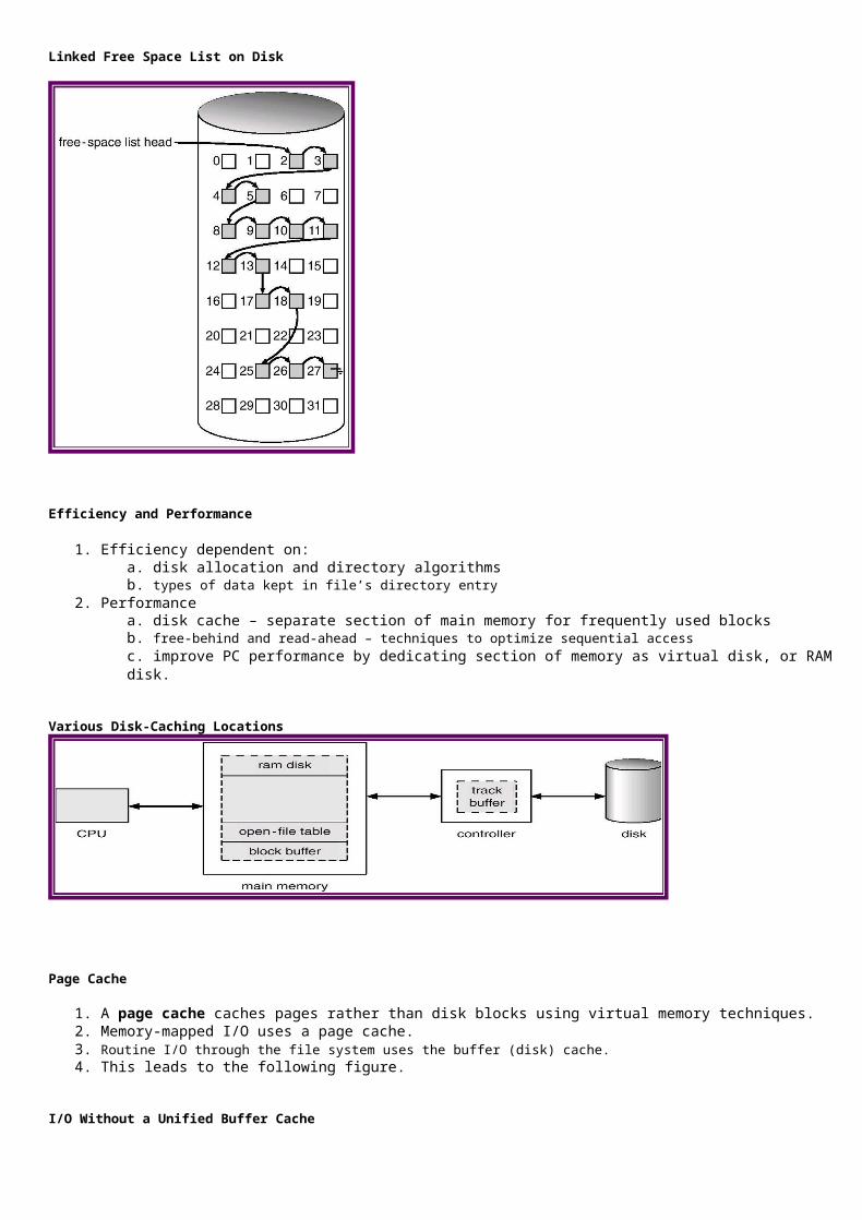
NPRCET-INFORMATION TECHNOLOGY
OS 1.139