CSIS Discussion Paper.105

Scenarios approach on the evaluation of a sustainable urban structure for reducing

carbon dioxide emission in Seoul City

by

Sohee Lee a* and Tsutomu Suzuki b

a* Corresponding author. Center for Spatial Information Science, University of Tokyo

5-1-5 Kashiwano-ha Kashiwa-shi Chiba, 277-8568, Japan

Email: shlee@csis.u-tokyo.ac.jp

b Graduate School of Systems and Information Engineering, University of Tsukuba

1-1-1 Ten-nodai Tsukuba Ibaraki, 305-8573, Japan

Email: tsutomu@risk.tsukuba.ac.jp

Abstract Many researchers have concerned on relationship and interaction between urban spatial structure and transportation system, moreover, brought to advance debates on environmental burden. In this paper, we estimate travel time of automobile and subway using GIS analysis, furthermore, a modal split model in terms of the modes. For using these results, we examine the reduction effect of carbon dioxide emission by assessing several scenarios which are about constructing subway infrastructure and reorganizing urban spatial structure. The result indicates that the policy direction for drawing up the urban spatial structure in terms of reducing carbon dioxide emission in Seoul City. The findings hold important implications for the policy debate surrounding sustainable urban system. 1 Introduction The issue of climate change has become a subject of intense interest all over the world since the last decade. The primary international policy framework against global warming is the United Nations Framework Convention on Climate Change (UNFCCC), specifically the Kyoto Protocol. In terms of the emphatic issue on preventing global warming is about reducing greenhouse gases. Expressly, it is essential to reduce the emission of carbon dioxide in handling climate change issue notably, because the emission of carbon dioxide is the largest contributing gas to the greenhouse effects (Fong et al, 2009; UN, 1998). Hence, an effort for reduction is necessary to strive in the variety fields also as a matter of urban system.

The concern of environmental impacts caused by urban activities in urban system has been identified. Many researchers have concerned on relationship and interaction between urban spatial structure and transportation system, moreover, brought to advance debates on environmental burden or transportation energy efficiency. For example, a first body of literature is concerned with the analysis of commuting distance (or time) to seeking for the relationship between urban structure and change of commuting behavior empirically (Aguilera, 2005; Rouwendal et al, 1994; Wachs et al, 1993). A second body of literature brings out the concept of excess commuting or wasteful commuting that represents the difference between actual and minimized commuting when distributions of jobs and housing is given as the same as present situation (Frost et al, 1998; Giuliano and Small, 1993; Ma and Banister, 2007; Merriman et al, 1995; White, 1988). A third body of literature is focused on jobs-housing mismatch in urban area physically to measure job accessibility as an indicator of auto-oriented urban structure (Kawabata and Shen, 2006; Kawabata, 2009). These studies have generated much discussion about the relationship between jobs-housing balance and commuting behavior in various ways. Furthermore, these studies have tried to verify a hypothesis that a polycentric urban model could contribute to reducing commuting distance (or time) by allowing workers to locate within or close to their workplace. As the results, commuting could not occurred efficiently all the time, namely workers do not always make a journey to workplace just reducing their commuting distance for some reasons. A forth body of literature is to clarify the debate concerning about the negative environmental and energy effects caused by transportation system and related urban density (Bertolini and Clercq, 2003; Cervero, 2001; Lee and Suzuki, 2007; Mindali et al, 2004; Newman and Kenworthy, 1989). A

lesson from these studies is commonly that energy consumption or environmental impact of urban transportation is negatively correlated with urban density. However, this is differently adopted into spatial hierarchy of urban area for example inner area and outer area. Additionally, some of approaches are modeled to integrate the effects of speed, acceleration, road grade and network, and also congestion to estimate the fuel consumption or emissions in relation to greenhouse gases (Frey H C et al, 2007; Nejadkoorki F et al, 2008; Scott D M et al, 1997). Nevertheless, these studies are not consistent with urban system and just focused on efficient of road networks.

Road transportation emission of carbon dioxide has received special attention, because they have been rising constantly. Although, there are methods through which they can be reduced, such as better transportation infrastructure, advances in vehicle technology and management systems, stabilizing carbon dioxide emission from road transport is likely to be a complicated task due to the rapidly rising traffic needs. According to the statistics of carbon dioxide emission of Korea in 2001, transportation section has captured 20 percents of total emission (generation of electric power: 30%, industry: 34%, domestic and commerce: 14%, and the rest). However, the annual average of transportation section is about 7 percents (specially, generation of electric power section is about 12.1 percents) which is compared to the emission ratio in 1990, and it is high and relatively recorded an increase tendency to exceed an average increase ratio (5.8%) in comparison with the other sections (KEEI, 2001).

In these perspectives, more detailed planning policy line for future urban spatial structure with appropriate evaluation approach is necessary. However, there is one more problem that is not simple to obtain proper personal traffic information even these data are valuable to utilize. For that reason, the purpose of this study is stated as two: (1) it is to suggest one of the way to estimate commuting time by modes and modal share for all origin-destination (OD) pairs of analyzed spatial units in Seoul City which data has not investigated but it is a fundamental and essential, moreover, (2) it is to clarify a policy direction to head for planning and organizing urban spatial structure with a little environmental load for the future in Seoul City.

This paper is organized as follows. The section 2 describes study area and data set. Then, the section 3 represents the estimation of commuting time and modal share by automobile and subway. Furthermore, the section 4 explains how to set the several scenarios, and its results are summarized with discussions. The conclusion includes the further works in the section 5. 2 Study area and data set The chosen study area for this study is Seoul City, Korea. The geographic unit applied is the smallest of administrative unit, named dong. Seoul City is divided into 522 dongs. The land area in Seoul City covers 605 square kilometer. In 2005 Seoul City accommodated 9,820 thousands peoples and that is occupied about a one-fifth of Korea, respectively, the number of workers is about 4,003 thousands (SK, 2005).

In this study, commuting (not to the other objective trips) is considered to examine the reduction of carbon dioxide emission by reorganizing residence and work places. Because, commuting to work is an important reason for travel in daily life, and also it occupied a big part of all objective trips. The number of worker (commuter) among origin-to-destination (OD) is available from the 2002 Seoul Metropolitan Region

Person Trip Survey (PT Survey) conducted by the Seoul Development Institute (SDI, 2002).

As we mentioned, origin-to-destination (OD) travel time is available, but it is sample-based, thus travel time for a complete set of OD pairs is generally not available. Researchers often estimate travel time in various ways when such data are needed for certain modes (Kawabata and Takahashi, 2005). In this study, as following Kawabata and Takahashi’s (2005) approach, we use Geographic Information System (GIS) to estimate the travel time and distance for journeys undertaken by automobile and subway. Many commuters also take the bus in Seoul City; however, the routes of bus lines in Seoul City and operation times are difficult to analyze because of a lack of data. Therefore, only automobile and subway are considered as modes. One problem is that the PT survey is 2 percents sample-based, and about 30 percents of sample is opened to the public. So that travel times by automobile and subway from the PT survey in 1996 and 2002 is combined to evaluate travel times by automobile and subway. Specifically, how to estimate travel time and distance illustrates by section 3.

To evaluate travel time and distance, the spatial data that the location of 522 dong offices (point), principle road lines, subway lines and stations are set. The point of dong offices is extracted from the numerical map of Seoul City conducted by the National Geographic Information Institute (NGII, 2000). Moreover, the principle road lines and subway lines and stations are offered by the Seoul Development Institute (SDI). Then, attribute information of subway lines and stations includes waiting time for train, transfer time and movement time between stations that is based on the service schedule of Seoul Metro and Seoul Metropolitan Rapid Transit Corporation are constructed (SM, 2002; SMRTC, 2002).

To measure the emission of carbon dioxide by riding automobile and subway among ODs, a unit which is defined as an amount of emission when one person moves 1km according to different transportation mode is adopted. In this study, a unit of carbon dioxide emission that we apply for evaluating the reduction of effect is 150.7 g-CO2 per person by 1km for automobile, and 17.9 g-CO2 per person by 1km for subway, and these figures is referred a report that is issued to the Korea Transport Institute (Lee et al., 2005). 3 Estimation of commuting times and modal share by automobile and subway The personal traffic information is utilized as an important data to draw up the future traffic demand estimation or prediction. It is also important for implementation the transportation plan and policy. There are two surveys in Korea to investigate the personal traffic information that are named the Population and Housing Census and the Person Trip Survey. However, in the Census data, spatial unit is large and items of questionnaire are not delicate. So, bias is possibly affected to the result of any analysis. In addition, the Person Trip survey is preformed as a sample for population of 2 percents. That is the reason of commuting times by all modes are not available for all the OD pairs, and also highly precise surveyed data is not offered. So that we estimate OD commuting times for trips between 522 dong offices. Commuting times by automobile and subway for all OD pairs (272,484= 522×522 pairs) are modeled using GIS (Kawabata and Takahashi, 2004, 2005). Moreover, we propose a modal split model by applying a binary logit model to estimate modal share for all OD pairs.

3.1 Estimating OD commuting times by using GIS As it was mentioned, the PT Survey is population of 2 percents sample-based, so it is not able to obtain a reasonable amount of commuting time data for enough OD pairs. To generate a reliable data set, commuting times of automobile and subway which are undertaken in 1996 and 2002 is pooled to estimate commuting times for all OD pairs. We take the following steps in estimating the commuting time of automobile, and all automobile users only follow the principle road lines will be assumed. As the first step, the direct distance between each dong office and its point of dong office from the nearest main road are calculated. Secondly, the shortest route by travel distance among the principle road lines is calculated. Thirdly, total distance among origin-to-destination is summed up the direct distance for office to the point of main road, the shortest route along the main road, and the point of main road to office.

We do not consider congestion-related delays because of a lack of data. We could have estimated the effect of traffic congestion by investigating the average speed; however, a limitation exists in that we were unable to consider the differences between central areas and local areas with serious traffic congestion and those areas with little congestion. Thus, we assume no traffic congestion. If the locations of the analyzed zones are close to each other, this assumption will lead to bias in the case of serious traffic congestion among zones; nevertheless, if the zones are located far from each other, the bias will be minimal because the effects of congestion are offset by parts of route with little congestion.

Next, we perform a regression analysis in which GIS-calculated OD commuting distance is adjusted using the actual commuting times reported in the PT Survey (using pooled data from 1996 and 2002). To convert the distance traveled by automobile to a commuting time, we use the following regression:

902.9039.0003.0016.0 +++= −− DofficeMainRoadj

Networkij

MainRoadOofficei

PTAutoij DDDT (1)

(2.106) (2.638) (20.920) (7.744) where PTAuto

ijT is the travel time of automobile reported in the PT Survey from zone i to

zone j, MainRoadOofficeiD − is the direct distance from origin office to the nearest main roads

in zone i, and NetworkijD is the shortest route from zone i to zone j, and DofficeMainRoad

jD − is the direct distance from the destination office to the nearest main roads in zone j. Adjusted R-square value: 0.552 (The numbers in parentheses indicate t values)

Table 1. Descriptive statistics of the adjusted OD commuting time of automobile Year Variables # of

observations Mean Std.Dev. Min. Max.

2002 GIS-calculated OD travel time 272,484 50.79 21.70 0.00 139.85 14,249 39.12 18.14 4.05 131.70

PT Survey OD travel time 14,249 43.42 23.22 0.00 420.00

The commuting times for all OD pairs were therefore adjusted and the relevant descriptive statistics are shown in Table 1. The mean commuting time in the PT Survey is considerably longer than that calculated by GIS; this is because we did not consider congestion-related delays in calculating the OD travel time. The GIS-calculated OD commuting time is therefore reasonably reliable in explaining the real world, even though the R2 value is a poor fit.

For subway users, three conditions are assumed. First, all subway users are assumed to walk to the stations. Second, any station within 1 kilometer radius of any dong office could be chosen to determine the shortest route to the destination because we assumed only within 1 kilometer (it is about 15 minutes on foot) could be reached on foot. Finally third, if there is no station is located within 1 kilometer of dong office, the nearest station is selected. Then, we take the following steps in estimating the commuting time of subway. First, the direct distance between dong offices and stations is calculated and it is converted to time using a walking speed of 4 kilometers per hour. Second, the shortest route among stations is calculated which is considered with not only travel time among stations, and also transfer time and waiting time for train among stations.

Next, we perform a regression analysis in which the GIS-calculated OD commuting times are adjusted using the actual travel times reported in the PT Survey. To compute the commuting time by subway, we estimate the following regression:

943.12708.0 += GISSubij

PTSubij TT (2)

(15.242) (9.061)

where PTSubijT is the travel time by subway reported in the PT Survey from zone i to

zone j, and GISSubijT is the shortest route time for zone i to zone j calculated using GIS.

Adjusted R-square value: 0.542 (The numbers in parentheses indicate t values) The commuting times for all OD pairs are adjusted, and result of descriptive

statistics is shown in Table 2. The mean of GIS-calculated OD commuting time is decreased. It means that newly constructed subway line contributed to decreasing commuting time.

Table 2. Descriptive statistics of the adjusted OD commuting time of subway Year Variables # of

observations Mean Std.Dev. Min. Max.

2002 GIS-calculated OD travel time 272,484 55.00 15.12 13.40 118.83 18,058 44.99 12.26 17.61 102.41

PT Survey OD travel time 18,058 45.85 22.29 0.00 660.00

3.2 Modal split model A modal split model by applying a binary logit model is purposed to evaluate modal share. In doing so, we use the commuting times of automobile and subway, as well as modal share determined from the PT survey undertaken in 2002. And also, the total number of trips by all modes which is estimated by SDI based on sample-based PT survey data. Moreover, two assumptions are made; first, only automobile or subway could be chosen when workers make a journey to their work place, and second, all workers choose the route to minimize the total commuting time.

The equation of modal split model is as follows:

})/(exp{11

CTTP

subautoauto ++

=μ

(3)

where autoP is ratio of sharing automobile, then, autoT is commuting time by automobile and subT is commuting time by subway.

We select OD pairs from the sample-based PT Survey undertaken in 2002 which are satisfied two conditions; first, the number of workers from origin to destination could be more than 5, and second, the ratio of modal share for automobile and subway could be potentially more than 50 percents. Figure 1 shows the proportion of commuters traveling by automobile plotted against the ratio of automobile to subway travel time, along with estimated curves. We then undertake a logistic regression analysis to estimate the parameters α and β . The form of logistic regression equation is as follows:

)}(exp{11

xPauto βα +−+

= (4)

where α is the constant of the equation and β is the coefficient of the predictor variable. In comparing equations (3) and (4), α corresponds to C, and β corresponds to μ . We perform a logistic regression using maximum likelihood estimation (MLE), in which the dependent variable is the modal share of automobile, and the independent variable is the ratio of travel times by automobile and subway (Table 3).

Table 3. Estimation of the values of α and β

Year α β

2002 2.70525 -3.01280

0

0.2

0.4

0.6

0.8

1

0 0.5 1 1.5 2 2.5

Rat

io o

f aut

omob

ile sh

are

(rat

io)

Ratio of time by automobile and subway use (ratio)Observed value in 2002 (n=606) Estimated value in 2002

Figure 1. Descriptive statistics of the adjusted OD travel time of subway

4 Scenarios set and its results 4.1 How to evaluate the reduction ratio of carbon dioxide emission of each scenario Figure 2 shows the process that how we evaluate the reduction ratio of carbon dioxide emission. First of all, we set up two parts of case: 1) in the first case, it is evaluated when infrastructure of public transportation is only invested within the same jobs and housing distribution as the present; 2) in the second case, how much carbon dioxide emission could be reduced by how to reorganize the distribution of residence and work places is evaluated.

Entropy Maximization Model(Objective function: entropy)

Commuting Minimization Problem(Objective function: time)

The flowvolumeScenarios set

Investing in infrastructureof public transportationReorganizingUrban spatial structure

input

Minimumtravel time

output

Parameter : Total travel time

Excess of the present

Excess

calculation comparison

output

input If calculated excess is same as the present, complete the processIf not, set total travel time and calculate again

Total CO2 emissioncalculation

repeat if not

Figure 2. Flow chart of evaluation scenario approach

For the first case, total carbon dioxide emission is simply calculated to apply commuting time of subway users which is newly estimated in the set period of 2010 and 2020 as the same way that is explained in section 3. However, we assumed that modal share of automobile and subway is the same as in 2002 for all OD pairs. Minutely, further explanation will be followed in section 4.2 (scenarios set). For the second case, we evaluate policy direction for making effective and strong urban spatial structure (distribution of residence and work places) in order to achieving lighten environmental burden. Total number of workers is not changed, however changing urban spatial

structure, namely reorganized number of workers in the place of residence and work, would bring on different pattern of commuting behavior. That is why we adopt the Entropy Maximization Model (EMM) to estimate the number of workers among all OD pairs. The EMM is one of the spatial interaction models, and it has been used as the foundation of model development in transportation since Wilson’s paper (for example, Kapur, 1982; Leung and Yan, 1997; Wang and Holguin-Veras, 2009; Webber, 1976). In this study, we adopt Wilson’s principle (Wilson, 1967), and the formulation is as follows:

∑ ∑−== =

m

i

n

jijij

ij

QQSQ 1 1}{

lnMax (5)

∑=

=n

jiij HQ

1s.t. (6)

∑ ==

m

ijij WQ

1 (7)

∑ ∑ ≤= =

m

i

n

jijij TQT

1 1 (8)

0≥Qij (9) where i and j are spatial units of residence and work places, ijQ is the number of commuting trips between i and j, ijT is the commuting time from origin i to destination j, T is the pre-specified total expenditure (in this study, it is commuting time), then, iH is the total out-flow (newly reorganized total number of housing) at i, jW is the total in-flow (newly reorganized total number of jobs) at j.

The problem of determination of number of trips ( ijQ ) is how to find that feasible state which would actually occur. The total number of ways of generating the feasible state (probability) is given by

∏∏= =

= m

i

n

jij

ij

Q

QQS

1 1

!

!)( (10)

The entropy maximization principle is to find all the feasible states which

satisfy all the constraints. Namely, the optimal solution of this model gives the most probable states distribution corresponding to the largest number of possible states assignments. Specifically, the most probable flow of OD pairs is obtained. The formulation above is composed of one objective function and four constraints. Statement (5) indicates that the objective is to find the most likely ways to distribute

commuting flows. Equation (6) and (7) ensure that there are no residence supply and jobs demand in each zone. In other words, the number of workers in the place of residence and work would be same as each scenario that we set. Equation (8) is the total commuting time constraint. Equation (9) is the nonnegative constraints which mean the resulting commuting flows should be equal or greater than zero.

The problem in this model is that the total commuting time is needed as a given factor. One of the ways simply takes the value of observation. However it is unknown because changing urban spatial structure also induces the different commuting behavior. In addition, the total time is effected by the variation of spatial distribution, for example, the jobs and housing distribution would be dispersed if the total cost is set bigger than the present cost that we do not know. Therefore, how to predict the total commuting time is a key point to solve the problem, so that we borrow the concept of excess commuting.

The excess commuting is concerned with the difference between the observed amount of commuting and a theoretical minimum amount of commuting time (or distance). A theoretical minimum is measured by the standard linear programming of transportation problem is defined as the Commuting Minimization Model (CMM) which is proposed by White (White, 1988), and the formulation is as follows:

∑ ∑== =

m

i

n

jijij

ij

TQTQ 1 1}{

Min (11)

∑ ==

n

jiij HQ

1s.t. (12)

∑ ==

m

ijij WQ

1 (13)

0≥Qij (14) where i and j are spatial units of residence and work place, ijQ is the number of commuting trips between i and j, ijT is the commuting time from origin i to destination j, then, iH is the total out-flow at i , jW is the total in-flow at j.

The formulation above is composed of one objective function and four constraints. Statement (11) indicates that the objective is to find the distribution of commuting flows in order to minimizing the total commuting time. Equation (12) and (13) ensure that no residence supply and jobs demand in each zone, namely it is the same as the present. Equation (14) restricts the decision variables to nonnegative values, so found commuting flows should be equal or greater than zero.

In the both of models (EMM and CMM), the commuting time between origin and destination is calculated by following equation:

MTMTT subij

subij

autoij

autoijij += (15)

where autoijT is the commuting time of automobile between i and j, sub

ijT is the

commuting time of subway between i and j, then, autoijM is the modal share of

automobile between i and j, subijM is the modal share of subway between i and j. The

way of evaluating the commuting times and modal share of automobile and subway is mentioned in section 3.

Then, the excess commuting is calculated as a proportion of the average actual commuting as follows:

actual

nmiactual

TTTExcess

.−= (16)

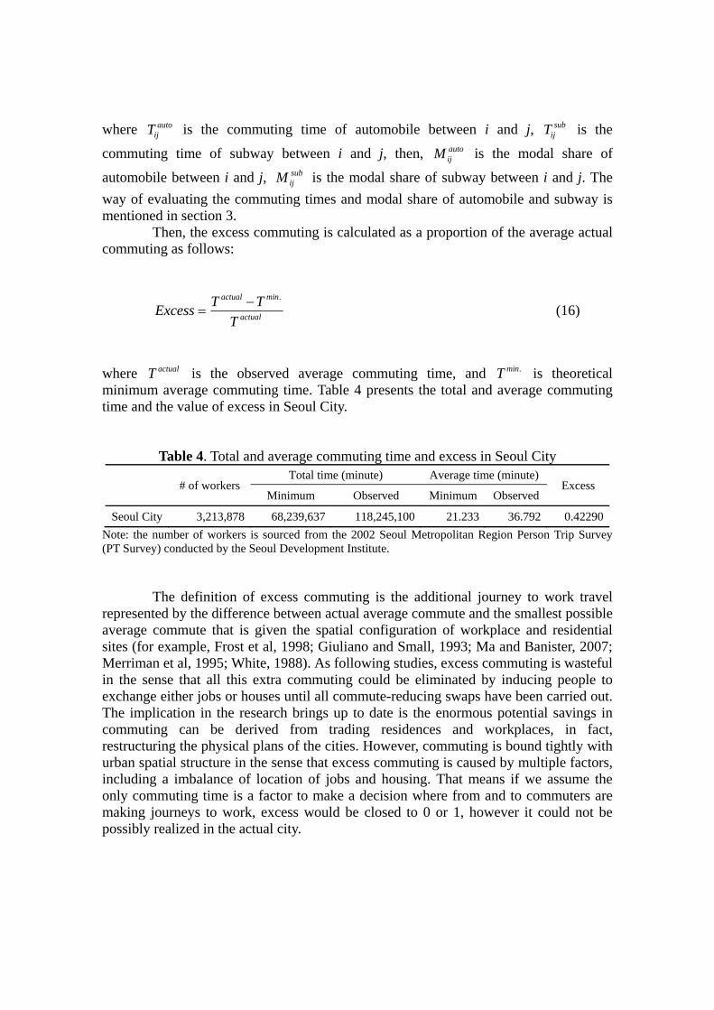
where actualT is the observed average commuting time, and .nmiT is theoretical minimum average commuting time. Table 4 presents the total and average commuting time and the value of excess in Seoul City.

Table 4. Total and average commuting time and excess in Seoul City

# of workers Total time (minute) Average time (minute)

Excess Minimum Observed Minimum Observed

Seoul City 3,213,878 68,239,637 118,245,100 21.233 36.792 0.42290 Note: the number of workers is sourced from the 2002 Seoul Metropolitan Region Person Trip Survey (PT Survey) conducted by the Seoul Development Institute.

The definition of excess commuting is the additional journey to work travel represented by the difference between actual average commute and the smallest possible average commute that is given the spatial configuration of workplace and residential sites (for example, Frost et al, 1998; Giuliano and Small, 1993; Ma and Banister, 2007; Merriman et al, 1995; White, 1988). As following studies, excess commuting is wasteful in the sense that all this extra commuting could be eliminated by inducing people to exchange either jobs or houses until all commute-reducing swaps have been carried out. The implication in the research brings up to date is the enormous potential savings in commuting can be derived from trading residences and workplaces, in fact, restructuring the physical plans of the cities. However, commuting is bound tightly with urban spatial structure in the sense that excess commuting is caused by multiple factors, including a imbalance of location of jobs and housing. That means if we assume the only commuting time is a factor to make a decision where from and to commuters are making journeys to work, excess would be closed to 0 or 1, however it could not be possibly realized in the actual city.

0

50,000,000

100,000,000

150,000,000

200,000,000

250,000,000

300,000,000

0.0 0.2 0.4 0.6 0.8 1.0

Total commuting time (minute)

Excess

Total commuting time: 118,245,100 minutes

Excess: 0.42290

Maximized total commuting time:263,390,803 minutes

Excess: 0.74092

Figure 3. Relationship between total commuting time and excess

Figure 3 presents the relationship between total commuting time and excess. As it shows, when the total commuting time becomes large, then the value of excess also becomes large within the same jobs and housing distribution because commuter makes a long journey. So we assume that the value of excess commuting would be calculated about the same or less comparing to the current value even if the urban spatial structure is changed, and the factors that affect to the commuting patterns are not changed or fixed as same as the present situation. Consequently, excess commuting would be decreased if a strategy tends to promote jobs-housing balance. That is the reason that the present value of excess is assumed as an evaluation standard even though the urban spatial structure is reorganized. In each scenario, the total commuting time constraint in the Entropy Maximization Model is determined by comparing the value of excess whether it is the same as the present value (=0.42290) or not. If it is not the same, the total commuting time is set and calculate again.

After that, the total carbon dioxide emission is calculated by the number of jobs and housing among OD pairs which is estimated by the Entropy Maximization Model. Then, the total carbon dioxide emission is compared to evaluate the effect of reorganizing urban spatial structure which one is more efficient to get rids of environmental burden. 4.2 Scenarios set Table 5 shows the description and condition of a moving worker for each scenario that we set. Scenarios are divided into two parts greatly. One part is to improve infrastructure of public transportation without reorganizing urban spatial structure (SA). In this study, we only consider subway and LRT as the public transportation. Other part is only to reorganize urban spatial structure with a current transportation condition (SB, SC, SD, SE).

Table 5. Description of scenarios and condition of a moving worker

Description The conditionof a moving worker (%)

Investing on infrastructure

SA1 Time period in 2010 for investing on subway lines 0%SA2 Time period in 2020 for investing on subway lines 0%

Reorganizing urban spatial

structure

SB1a

Concentration on urban center 10%

b 15%c 30%

SB2a

Concentration on urban and suburban centers 5%

b 15%c 30%

SB3a

Concentration on urban, suburban and local centers 10%

b 20%c 30%

SC1a

Promotion of residence area in urban center 10%

b 20%c 30%

SC2a

Promotion of residence area in urban and suburban centers

10%b 20%c 30%

SD1a Promotion of developing area in near of station

considering with jobs-housing balance (Distance to station is within 500m)

10%b 20%c 30%

SD2a Promotion of developing area in near of station

considering with jobs-housing balance (Distance to station is within 1,000m)

10%b 20%c 30%

SE1a Concentration on the number of jobs and residence in

areas where is both urban and suburban centers, in addition, near subway station (within 500m)

5%b 10%c 15%

SE2a Concentration on the number of jobs and residence in

areas where is both urban, suburban and local centers, in addition, near subway station (within 500m)

5%b 10%c 15%

SE3a

Concentration on the number of jobs and residence in areas where is near subway station (within 500m)

5%b 10%c 15%

For scenario A, we name it as SA, is the case for investing in construction of public transportation infrastructure without changing urban spatial structure. It evaluates the reduction effect of carbon dioxide emission by only maintenance and construction of the public transportation system. SA is set for the time periods in 2010 and 2020 (SA1 and SA2) as the standard criterion when the public transportation infrastructure invested. Table 6 shows the network of subway and LRT, and its planned service year in Seoul City, and figure 4 presents its spatial distribution (TSC, 2007). Travel time and modal share of automobile and subway are estimated by using GIS network analysis. The process of estimation is the same as in section 3.

For scenarios B, C, D, and E, we name it as SB, SC, SD, and SE, are the case for reorganizing urban spatial structure only with a current public transportation

condition. Mainly four cases are set up: (1) concentration / dispersion of jobs on urban, suburban or local centers (SB), (2) promotion of residence area in urban and suburban centers (SC), (3) promotion of developing area in near of station considering with jobs-housing balance (SD), (4) concentration on the number of jobs and residence in areas where is both urban and suburban centers, and also where is near subway station (SE).

Table 6. The plan of constructing subway lines and LRT in Seoul City Planned opening year Name of line

2003 Bundang line

2006 Extended line No. 1

2008 Extended Bundang line

2009 Extended line No. 3

2011 Extended line No. 9

2011 New Bundang line

2017 Light Rail Transit(LRT)

Dongbuk line

Mokdong line

Myumok line

Seobu line

Shinrim line

Wooi line Note: Airport railway between Kimpo airport and Seoul station that is planned to operate in 2011 is excluded from the analysis.

We consider reorganization of urban spatial structure with concentration or decentralization of workers in that area of urban, suburban, or local centers. The location of those areas is specified as the fundamental idea in 2020 Seoul City Comprehensive Plan, it shows in figure 5 (SC, 1998). In terms of comprehensive plan, urban spatial structure in Seoul City is intended to be polycentric-dispersion spatial structure, and also reinforce with a center for each sphere of life (namely local center). By aiming to such spatial structure, first, commuting will disperse to the suburban and/or local center for good side of effect. Second, by strengthening functions in a sphere of life and well equipping public transportation, proximity of jobs and housing could be induced. It would be directly connected to save travel time or distance. Farther, it induces to reduce transportation energy and carbon dioxide emission. Nevertheless, the effect of modified urban spatial structure is not quite evaluated quantitatively somehow, moreover, it is required.

0 2 4 6 8 101km±

Boundary of 25-ward areaStations by 2002Lines by 2002Stations newly constructed by 2020Lines newly constructed by 2020

Figure 4. The network of subway and LRT in 2002 and the future

±

Boundary of smallest administrative unit (Dong)

Boundary of 25-ward area

Urban center

5-suburban center

15-local center

Yeongdeungpo

Yeongdong

Wangsimni

Yongsan

Sangam

0 2 4 6 8 101km

Figure 5. The division of spatial hierarchy by 2020 Seoul City Comprehensive Plan

Table 7. The results of evaluating scenarios

Results Reduced

ratio of CO2 (%)

Required CO2 emission

(g-CO2/person)

Required commuting time

(min/person)

Required commuting dist.

(km/person)

Ratio of reorganized workers (%)

Ratio of modal share (%)

residence workplace auto subway Present state - 470.13 36.79 8.442 not changed not changed 40.66 59.34 Scenarios set

Investing on infrastructure

SA1 -4.5 449.07 37.86 7.590 not changed not changed 40.66 59.34 SA2 -6.0 441.85 35.68 7.122 not changed not changed 40.66 59.34

Reorganizing urban spatial

structure

SB1a 0.3 473.11 36.87 8.280 0.00 1.66 39.64 60.36 b 1.2 477.17 37.07 8.370 0.00 2.39 39.55 60.45 c 2.6 483.88 37.41 8.523 0.00 4.79 39.36 60.64

SB2a 0.7 474.83 36.95 8.313 0.00 0.73 39.65 60.35 b 4.5 492.69 37.84 8.708 0.00 4.18 39.28 60.72 c 9.2 515.14 38.96 9.210 0.00 8.36 38.79 61.21

SB3a 4.8 494.21 37.92 8.754 0.00 5.42 39.20 60.80 b 9.8 517.72 39.09 9.295 0.00 10.84 38.61 61.39 c 14.9 541.75 40.30 9.863 0.00 16.26 37.95 62.05

SC1a -0.3 470.32 36.73 8.216 0.20 0.00 39.73 60.27 b -0.5 469.10 36.66 8.189 0.39 0.00 39.76 60.24 c -0.8 467.88 36.60 8.163 0.59 0.00 39.78 60.22

SC2a -1.0 466.76 36.55 8.140 0.79 0.00 39.78 60.22 b -2.0 461.97 36.31 8.038 1.58 0.00 39.85 60.15 c -3.0 457.21 36.06 7.937 2.37 0.00 39.93 60.07

SD1a -2.3 460.91 36.27 8.034 1.26 1.72 39.77 60.23 b -11.7 416.44 34.19 7.116 2.52 3.44 40.32 59.68 c -13.4 408.30 33.79 6.969 3.78 5.16 40.32 59.68

SD2a -9.8 425.53 34.62 7.299 2.08 3.52 40.27 59.73 b -11.2 418.85 34.28 7.198 4.15 7.03 40.22 59.78 c -12.2 414.14 34.04 7.142 6.23 10.55 40.11 59.89

SE1a -2.1 461.88 36.31 8.074 5.00 5.00 39.59 60.41 b -4.1 452.32 35.83 7.908 10.00 10.00 39.50 60.50 c -6.1 442.90 35.35 7.744 15.00 15.00 39.43 60.57

SE2a -2.3 460.81 36.30 8.069 5.00 5.00 39.55 60.45 b -4.5 450.22 35.80 7.899 10.00 10.00 39.38 60.62 c -6.7 439.80 35.32 7.733 15.00 15.00 39.22 60.78

SE3a -0.5 469.21 36.70 8.274 5.00 5.00 39.30 60.70 b -0.9 467.44 36.63 8.323 10.00 10.00 38.86 61.14 c -1.1 466.45 36.61 8.396 15.00 15.00 38.37 61.63

The detail explanation of each scenario is as follows. First, the reduction of carbon dioxide emission is assessed in the case of concentration or dispersion type of commercial and business functions (SB). Some portion of jobs is moved to urban, suburban and/or local centers. The number of jobs is mainly concentrated in urban center (SB1), and urban and suburban centers are reinforced by moving the number of jobs (SB2). Then, we consider local centers of sphere as well (SB3). Second, promotion of residence area in urban or suburban centers is evaluated (SC). The number of residence is promoted to develop in urban center (SC1), moreover, movement of residence occurs not only urban center but suburban centers (SC2). Third case that area where the use of subway is convenient is promoted to develop with considering jobs-housing balance is assessed (SD). Administrative zones (dongs) within the boundary of 500m from subway station are targeted to adjust jobs-housing balance (SD1). Moreover, the area within the boundary of 1,000m from subway station is also concerned to develop lively considering with jobs-housing balance (SD2). Fourth case that the both of jobs and housing are moved to zones where is in near of subway station and also the centers is estimated (SE). In detail, urban and suburban centers are focused on developing as concentration area with sufficient condition of the boundary of 500m from the station (SE1). Then, urban, suburban and local centers of sphere are focused (SE2). Furthermore, zones where only are within 500m to station are considered (SE3). The percentage of moved jobs and housing for each scenario is presented in table 5. 4.2 Findings and discussions First, we present results for the reduction ratio of carbon dioxide emission and ratio of reorganized workers by the place of work and residence. From this results, we could evaluate how much of total carbon dioxide emission could be reduced by reorganizing urban spatial structure. Next, we present results for the change in spatial distribution of work and residence places. From this results, we could find out the policy direction that how to reorganize urban spatial structure to cut down the environmental burden in the future. Table 7 shows the evaluation result by each scenario. In this study, we evaluate each scenario as comparing with the reduced ratio of carbon dioxide emission and ratio of moved number of jobs and residence.

In the result of SA, about 4.5% in 2010 year (SA1) and 6.0% in 2020 year (SA2) of carbon dioxide emission compare to the present commuting behavior could be reduced even we do not reorganize urban spatial structure by newly equipping infrastructure of public transportation network. In other words, as the current urban spatial structure, some of carbon dioxide reduction is expected. We assume that the ratio of modal share is same as in 2002, even though the network is newly built. Consequently, the reduction ratio of carbon dioxide emission could be much larger than the result.

In the result of SB which is focused on concentration or dispersion type of business function, the reduction ratio of carbon dioxide emission is calculated greater than the present condition. Moreover, the reduction ratio presents higher percentage when reorganized number of workers became big. The policy to make the strong urban and suburban centers is potentially to bring out the long journey from work to residence place, thus it makes the ratio of carbon dioxide emission is increased. In other words, depending on the commuting behavior could be occurred much worse conversely.

In the result of SC which is focused on promotion of residence area in urban or suburban centers, the reduction effect of carbon dioxide emission was presented. As the result of SC2a shows 3% of total carbon dioxide emission decreased when about 2.4 % of workers in the place of residence in urban and suburban centers is reorganized. Indeed, the reduction ratio of carbon dioxide emission seems to grow big so that the number of workers in the place of residence becomes large portion. In other words, as for the policy of the residence promotion in urban center and suburban centers, the reduction effect was provided by shortening commuting to the work place. It could be proved to compare the change of commuting distance which was about 8.44km in the present condition of 2002, and it becomes shorter in this scenario.

The largest reduction of carbon dioxide emission makes an appearance in the result of SD which is focused on promoting the area in near subway station with considering jobs-housing balance. As a result, SD1c shows about 13.4% (the number of workers in the place of jobs and residence was about 3.78% and 5.16) and SD2c appears about 12.2 % (the number of workers in the place of jobs and residence was about 6.23% and 10.55%) of the reduction ratio of carbon dioxide emission. It explains that the policy of promoting the area where is much convenient to access subway station (such as Transit-Oriented Development (TOD)) shows good side of effect to reduce environment impacts. Even though only small portion of number of workers in the place of residence and workplace is reorganized it provides the big portion of reduction. Moreover, larger amount of reduction was gained when the area within the boundary of 500m to subway station was intensively considered. It explains that selected area where is especially good accessibility is desirable to intensively develop as a foothold area.

In the result of SE which is focused on concentration on the number of jobs and residence in areas where both urban center and near subway stations are, the reduction effect of carbon dioxide emission was presented. From such a result, the policy of promoting the areas in near of subway station and in where is urban center or suburban centers have been also effective to reduce the emission of carbon dioxide. However, comparing the results of SD and SE, such areas are better to establish the plan for mixed land use while considering jobs-housing balance, not only as the place of residence or even work place.

0 2 4 6 8 101km

±

Density of jobs(jobs / sp. km)

(max. 903.3)

0.0 - 40.0

40.1 - 80.0

80.1 - 120.0

120.1 - 160.0160.1 - 200.0

over 200.0

Yeongdeungpo

Yeongdong

Urban Center

0 2 4 6 8 101km

±

Density of workers(workers / sp. km)

(max. 220.5)

0.0 - 40.0

40.1 - 80.0

80.1 - 120.0

120.1 - 160.0

160.1 - 200.0

over 200.0

Figure 6. The density of jobs and workers in Seoul City

0 2 4 6 8 101km

±

Change of jobs (%)(SD1-c)

Subway lines in 2002

below 0.00 (min. -10.15)

0.00

over 0.00 (max. 30.04)

Stations

0 2 4 6 8 101km

±

Change of workers (%)(SD1-c)

Subway lines in 2002

below 0.00 (min. -6.66)

0.00

over 0.00 (max. 30.02)

Stations

Figure 7. Change of jobs and workers distribution by SD1-c

Next, we present the density distribution of jobs and workers in the place of work and residence places in Seoul City, and also the change in spatial distribution of moved jobs and workers that is the result of SD1-c showed the largest reduction ratio of carbon dioxide emission from the set scenarios. To present these maps typically, we could find out how to distribute spatially jobs and workers to achieve the reduction of carbon dioxide emission. Figure 6 shows the density of jobs and workers. As it shows clearly, Seoul City is distinctive polycentric urban structure. Jobs are concentrated on the urban center that is the central part of Seoul City and two suburban centers which are Yeongdeungpo and Yeongdong, however, workers are decentralized. This means that sometimes the workers make a long journey to work because jobs and housing is not balanced. That is why scenario that the promotion of residence area in urban center or urban and suburban center represented a small portion of carbon dioxide reduction caused by improving jobs-housing balance in urban and suburban center (SC). Figure 7 presents the change of moved jobs and workers in SD1-c. In this scenario, the reduction ratio of carbon dioxide emission was 13.4 %. A few tendencies show how to rearrange jobs and workers distribution reduce carbon dioxide emission could be found. First, it is better to decentralize the workers in place of workplace where are more handy to use the public transportation. In other words, promotion of local centers is induced to disperse the commuting and it caused to reduce their travel cost. Moreover, it possibly makes their journey short (the top side of map in figure 7). Second, it is important to secure the place of residence in that area where showed the high jobs density (urban and suburban center). Nevertheless, the area with good accessibility to station is needed to promote as the residential area because it makes easy to commute (the bottom side of map in figure 7). 5 Conclusion In this paper, we estimated travel time of automobile and subway by using GIS analysis, moreover, a modal split model in terms of the modes. For using these results, we examined the reduction effect of carbon dioxide emission by assessing several scenarios which are about constructing subway infrastructure and reorganizing urban spatial structure.

From the results, we could find the meaningful policy direction for drawing up urban spatial structure in terms of reducing carbon dioxide emission. First, long distance commuting could be reduced by promoting residential density where employment density is high. Second, the area where are accessibility to the station is good enough and especially modal share of subway is high as needed to develop mainly, it is needed to pick up the foothold area to promote chiefly where is convenient to access the subway station. In addition, jobs-housing balance of employment and residence is needed to be considered compositely.

Further research remains to be carried out. First, set scenarios in this study were quite simple based, because we tried to bring the direction of policy forth that how we need to draw up urban spatial structure for the future. Moreover, estimation for quantitative value of development in Seoul City is not simple. We need to consider of that with micro analysis. Second, the emission of carbon dioxide was considered as cost only. However, construction cost of subway infrastructure or cost for changing urban spatial structure are also important to be considered. All scenarios are needed to be

assessed by reducing the total cost to compare the efficiency. In addition, the value for trade-off between cost and construction time are needed to analyze. Third, for the sake of simplicity only automobile and subway were considered. However, according to attain a more realistic analysis, it is necessary to consider other modes of transportation, especially given the high ratio of bus use in Seoul City. Acknowledgements Reference Aguilera A, 2005, “Growth in commuting distances in French polycentric metropolitan

areas: Paris, Lyon and Marseille” Urban Studies 42(9) 1537-1547 Bertolini L, Clercq F, 2003, “Urban development without more mobility by car: lessons

from Amsterdam, a multimodal urban region” Environment and Planning A 35 575-589

Cervero R, 2001, “Efficient urbanisation: economic performance and the shape of the metropolis” Urban Studies 38(10) 1651-1671

Fong W, Matsumoto H, Lun Y, 2009, “Application of system dynamics model as decision making tool in urban planning process toward stabilizing carbon dioxide emissions from cities” Building and Environment 44 1528-1537

Frey H C, Rouphail N M, Zhai H, Farias T L, Goncalves G A, 2007, “Comparing real-world fule consumption for diesel- and hydrogen-fueled transit buses and implication for emissions” Transportation Research D 12 281-291

Frost M, Linneker B, 1998, Excess or wasteful commuting in a selection of British cities” Transportation Research A 32(7) 529-538

Giuliano G, Small K, 1993, “Is the journey to work explained by urban structure?” Urban Studies 30(9) 1485-1500

Kapur J N, 1982, “Entropy maximisation models in regional and urban planning” International Journal of Mathematical Education in Science and Technology 13(6) 693-714

Kawabata M, Takahashi A, 2005, “Spatial dimensions of job accessibility by commuting time and mode in the Tokyo Metropolitan Area” Theory and applications of GIS 13(2) 139-148

Kawabata M, Shen Q, 2006, “Job accessibility as an indicator of auto-oriented urban structure: a comparison of Boston and Los Angeles with Tokyo” Environment and Planning B 33 115-130

Kawabata M, 2009, “Spatiotemporal dimensions of modal accessibility disparity in Boston and San Francisco” Environment and Planning A 41 183-198

KEEI, 2001, “Statistical data for greenhouse gases emission in Korea” Korea Energy Economics Institute, http://www.keei.re.kr/main.nsf/index.html

Lee S, Kwon T, Kwon H, 2005, “The effect analysis on greenhouse gas reduction policy in the transportation sector to prepare for climate change agreement” a report of the Korea Transport Institute (in Korean)

Lee S, Suzuki T, 2007, “GIS-based analysis of advantageous zones for transit-oriented development in Seoul” Proceedings of the International Symposium on Urban Planning 2007 (ISUP2007), 287-296 Leung Y, Yan J, 1997, “A note on the fluctuation of flows under the entropy principle”

Transportation Research B 31(5) 417-423

Ma, K and Banister D, 2007, “Urban spatial change and excess commuting” Environment and planning A 39 630-646

Merriman D, Ohkawara T, Suzuki T, 1995, “Excess commuting in the Tokyo metropolitan area: measurement and policy simulations” Urban Studies 32(1) 69-85

Mindali O, Raveh A, Salomon I, 2004, “Urban density and energy consumption: a new look at old statistics” Transportation Research A 38 143-162

Nejadkoorki F, Nicholson K, Lake I, Davies T, 2008, “An approach for modeling CO2 emissions from road traffic in urban areas” Science of the Total Environment 406 269-278

Newman P, Kenworthy J, 1989, “Gasoline consumption and cities: a comparison of US cities with a global survey” Journal of the American Planning Association 55 23-37

NGII, 2000, “The numerical map of Seoul” the National Geographic Information Institute, http://www.ngii.go.kr/

Rouwendal J, Rietveld P, 1994, “Changes in commuting distances of Dutch households” Urban Studies 31(9) 1545-1557

SC, 1998, “2020 Seoul City comprehensive plan” Seoul City, http://www.seoul.go.kr/2004brief/2020/city_main.html

Scott D M, Kanaroglou P S, Anderson W P, 1997, “Impacts of commuting efficiency on congestion and emissions: case of the Hamilton CMA, Canada” Transportation Research D 2(4) 245-257

SDI, 2002, “2002 Seoul metropolitan region person trip survey”, Seoul Development Institute, http://www.sdi.re.kr/poup/trff/trff_idx.jsp

SK, 2005, “2005 Population and Housing Census of Korea”, Statistics Korea, http://www.kostat.go.kr/nso_main/nsoMainAction.do?method=main&catgrp=eng2009

SM, 2002, “Operating timetable of trains and transfer times for line Nos. 1 to 4”, Seoul Metro, http://www.seoulmetro.co.kr/index.jsp

SMRTC, 2002, “Operating timetable of trains and transfer times for line Nos. 5 to 8” Seoul Metropolitan Rapid Transit Corporation, http://www.smrt.co.kr/english_smrt/ndex.jsp

TSC, 2007, “2020 Seoul city transportation plan” Transport Seoul City, http://transport.seoul.go.kr/

UN, 1998, “Kyoto protocol to the united nations framework convention on climate change”, United Nations, http://unfccc.int/kyoto_protocol/items/2830.php

Wachs M, Taylor B D, Levine N, Ong P, 1993, “The changing commute: a case study of the jobs-housing relationship over time” Urban Studies 30(10) 1711-1729

Wang Q, Holguin-Veras J, 2009, “Tour-based entropy maximisation formulations of urban commercial vehicle movements” The 18th International Symposium on Transportation and Traffic Theory, 16-18 July 2009 at Hongkong

Webber M J, 1976, “Entropy maximizing models for the distribution of expenditures” Papers in Regional Science 37(1) 185-198

White M J, 1988, “Urban commuting journeys are not wasteful” Journal of Political economy 96 1097-1110

Wilson A G, 1967, “A statistical theory of spatial distribution model” Transportation Research 1 253-269