Embed Size (px)
Citation preview
CUDA for Real‐Time MultigridFinite Element Simulation ofSoft Tissue DeformationsSoft Tissue Deformations
Christian Dick
Computer Graphics and Visualization GroupComputer Graphics and Visualization Group
Technische Universität München, Germany
computer graphics & visualization
MotivationR l ti h i b d i l ti f d f bl bj t• Real‐time physics‐based simulation of deformable objects– Various applications in medical surgery training and planning
• Finite element method (FEM) in combination with a geometric multigrid solver( ) g g– Physics‐based material constants
– Mathematically sound
Easy handling of boundaries– Easy handling of boundaries
– Linear‐time complexity of the solver in the number of unknowns
• Goal: Exploit the GPU’s massive computing power and memory bandwidth to significantly increase simulation update rates / increase FE resolution
computer graphics & visualizationGTC 2010 Christian Dick, [email protected]
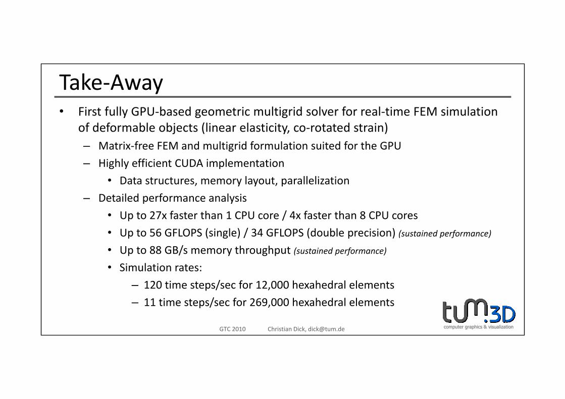
Take‐AwayFi t f ll GPU b d t i lti id l f l ti FEM i l ti• First fully GPU‐based geometric multigrid solver for real‐time FEM simulation of deformable objects (linear elasticity, co‐rotated strain)– Matrix‐free FEM and multigrid formulation suited for the GPU
– Highly efficient CUDA implementation
• Data structures, memory layout, parallelization
– Detailed performance analysisDetailed performance analysis
• Up to 27x faster than 1 CPU core / 4x faster than 8 CPU cores
• Up to 56 GFLOPS (single) / 34 GFLOPS (double precision) (sustained performance)
• Up to 88 GB/s memory throughput (sustained performance)
• Simulation rates:
– 120 time steps/sec for 12,000 hexahedral elements
computer graphics & visualizationGTC 2010 Christian Dick, [email protected]
p / ,
– 11 time steps/sec for 269,000 hexahedral elements
Deformable Objects on the GPUA hit t f th NVIDIA F i GPU• Architecture of the NVIDIA Fermi GPU– 15 multiprocessors, each with 32 CUDA cores (ALUs) for integer‐ and floating‐point
arithmetic operations
– GPU executes thousands of threads in parallel
• Requirements for an algorithm to run efficiently on the GPU– Restructure algorithm to expose fine‐grained parallelismRestructure algorithm to expose fine grained parallelism
(one thread per data element)
– Avoid execution divergence of threads in the same warp
Ch l t hi h bl l i f d i– Choose memory layouts which enable coalescing of device memory accesses
– Only threads in the same thread block can communicate and be synchronized efficiently (global synchronization only via separate kernel calls)
computer graphics & visualizationGTC 2010 Christian Dick, [email protected]
– Very limited resources (registers, shared memory) per thread
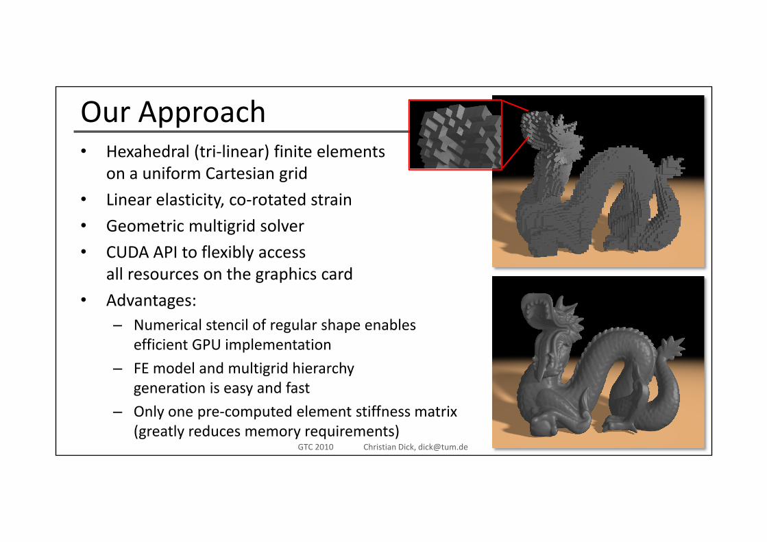
Our ApproachH h d l (t i li ) fi it l t• Hexahedral (tri‐linear) finite elementson a uniform Cartesian grid
• Linear elasticity, co‐rotated strain
• Geometric multigrid solver
• CUDA API to flexibly accessall reso rces on the graphics cardall resources on the graphics card
• Advantages:– Numerical stencil of regular shape enablesg p
efficient GPU implementation
– FE model and multigrid hierarchygeneration is easy and fast
computer graphics & visualizationGTC 2010 Christian Dick, [email protected]
g y
– Only one pre‐computed element stiffness matrix(greatly reduces memory requirements)
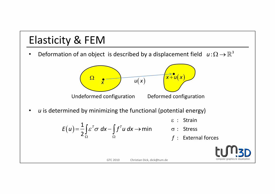
Elasticity & FEMD f ti f bj t i d ib d b di l t fi ld 3Ω• Deformation of an object is described by a displacement field 3:Ω→u
( )Ω ( )u xx( )x u x+
Undeformed configuration Deformed configuration
• u is determined by minimizing the functional (potential energy)
Undeformed configuration Deformed configuration
St i
( ) 1min
2T TE u dx f u dx
Ω Ω
= − →∫ ∫ε σ: Strain
: Stress
: External forcesf
εσ
computer graphics & visualizationGTC 2010 Christian Dick, [email protected]
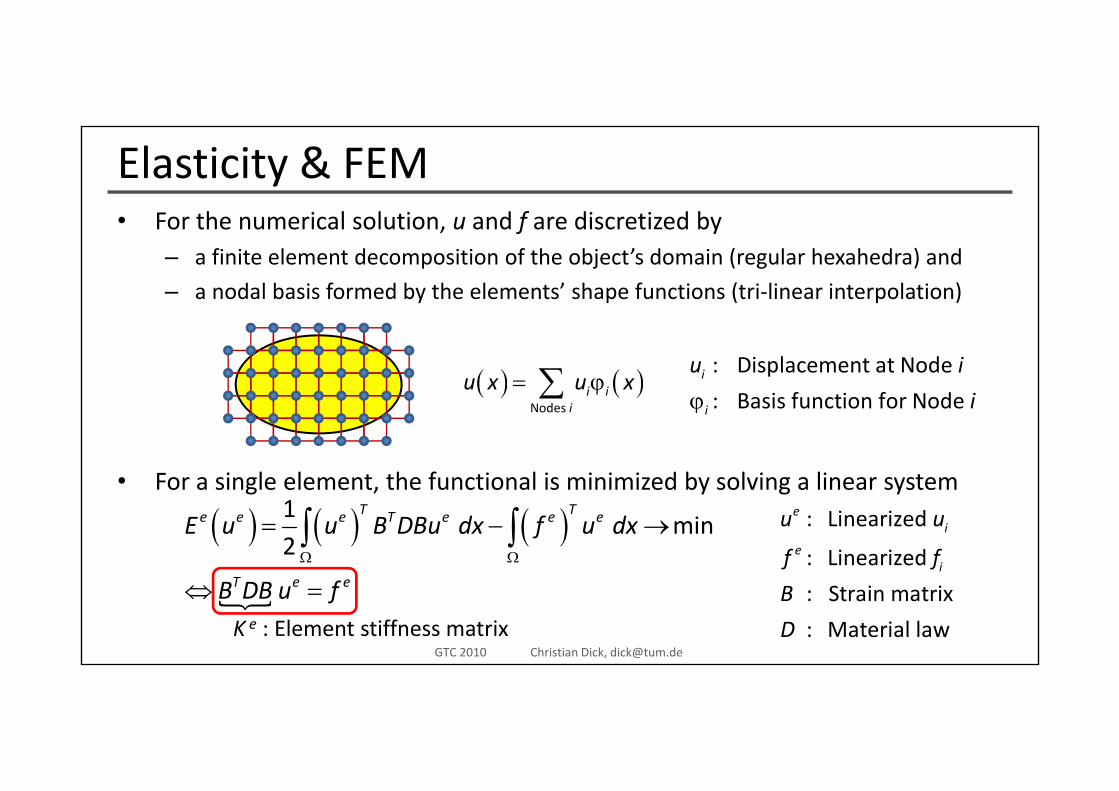
Elasticity & FEMF th i l l ti d f di ti d b• For the numerical solution, u and f are discretized by– a finite element decomposition of the object’s domain (regular hexahedra) and
– a nodal basis formed by the elements’ shape functions (tri‐linear interpolation)
( ) ( )i iu x u x= ϕ∑: Displacement at Node
B i f ti f N diu i
i
• For a single element the functional is minimized by solving a linear system
( ) ( )Nodes
i ii
∑ : Basis function for Node i iϕ
For a single element, the functional is minimized by solving a linear system
( ) ( ) ( )1min
2
T Te e e T e e eE u u B DBu dx f u dxΩ Ω
= − →∫ ∫ : Linearized
: Linearized
ei
ei
u u
f f
computer graphics & visualizationGTC 2010 Christian Dick, [email protected]
T e eB DB u f⇔ = : Strain matrix
: Material law
B
DK e : Element stiffness matrix
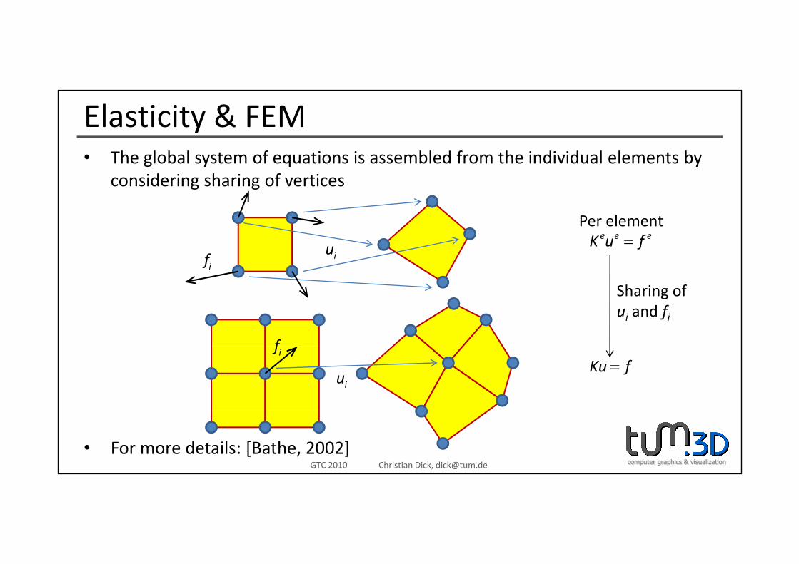
Elasticity & FEMTh l b l t f ti i bl d f th i di id l l t b• The global system of equations is assembled from the individual elements by considering sharing of vertices
P l t
ifiu
e e eK u f=Per element
f
Sharing ofui and fi
Ku f=if
iu
computer graphics & visualizationGTC 2010 Christian Dick, [email protected]
• For more details: [Bathe, 2002]
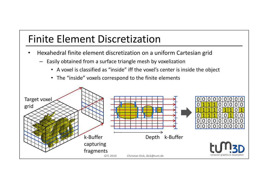
Finite Element DiscretizationH h d l fi it l t di ti ti if C t i id• Hexahedral finite element discretization on a uniform Cartesian grid– Easily obtained from a surface triangle mesh by voxelization
• A voxel is classified as “inside” iff the voxel’s center is inside the object
• The “inside” voxels correspond to the finite elements
0 0 0 0 0 00 1 1 1 0 01 1 1 1 0 10 1 1 1 0 0
0 0 00 0 01 0 11 0 0
Target voxelgrid
0 1 1 1 0 00 0 0 0 0 00 0 0 0 0 0
1 0 00 0 00 0 0
k‐Buffer k‐BufferDepth
computer graphics & visualizationGTC 2010 Christian Dick, [email protected]
k‐Buffercapturingfragments
k‐BufferDepth
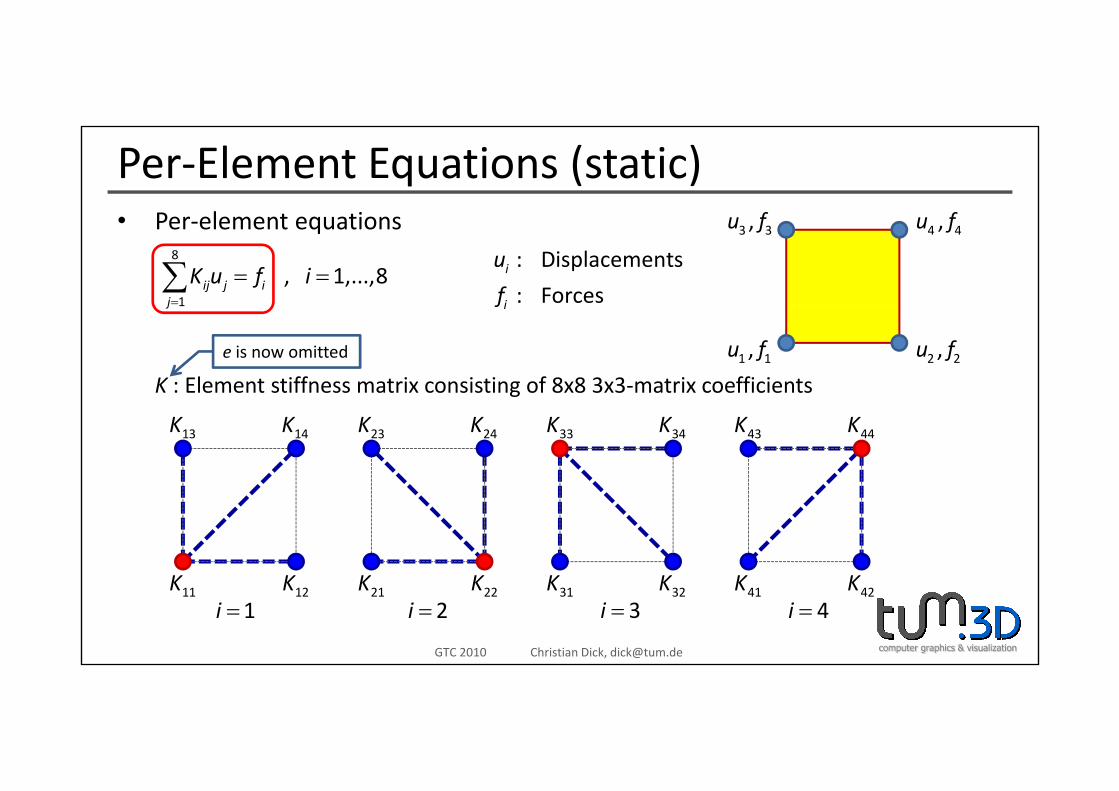
Per‐Element Equations (static)P l t ti f f• Per‐element equations
8
1
, 1,...,8=
= =∑ ij j ij
K u f i
3 3,u f 4 4,u f
: Displacements
: Forcesi
i
u
f1j
1 1,u f 2 2,u f
K : Element stiffness matrix consisting of 8x8 3x3‐matrix coefficients
e is now omitted
if
g
13K 14K 23K 24K 33K 34K 43K 44K
K K K K K K K K
computer graphics & visualizationGTC 2010 Christian Dick, [email protected]
1i =11K 12K
2i =21K 22K
3i =31K 32K
4i =41K 42K
Per‐Element Equations (co‐rotated, static)C t t d t i Rotate forces from initial into current configuration• Co‐rotated strain
( )( )8
0 0 , 1,...,8Tij j j j iRK R p u p f i+ − = =∑ : Element rotationR
Rotate displacements back into initial configuration
Rotate forces from initial into current configuration
0: Undeformed vertex positionsp( )
( )1
8 80 0
1 1ˆ
j
T Tij j i ij j j
j jA
RK R u f RK R p p
=
= =
= − −∑ ∑
: Undeformed vertex positionsjp
• R is obtained by polar decomposition of the element’s average deformation
ˆij
i
Ab
Linear strain Linear, co‐rotated strainy p p g
gradient (5 iterations)8
0 3
1 1 1 1, ,
4⎛ ⎞= + ± ± ±⎜ ⎟⎝ ⎠
∑ oldiR I u
a b c( ),− + ( ),+ +
, , : Edge lengths of hexahedral element
Signs :
a b c
computer graphics & visualizationGTC 2010 Christian Dick, [email protected]
( )( )1
11
412
=
−+
⎝ ⎠
= +
i
T
n n n
a b c
R R R ( ),− − ( ),+ −x
y
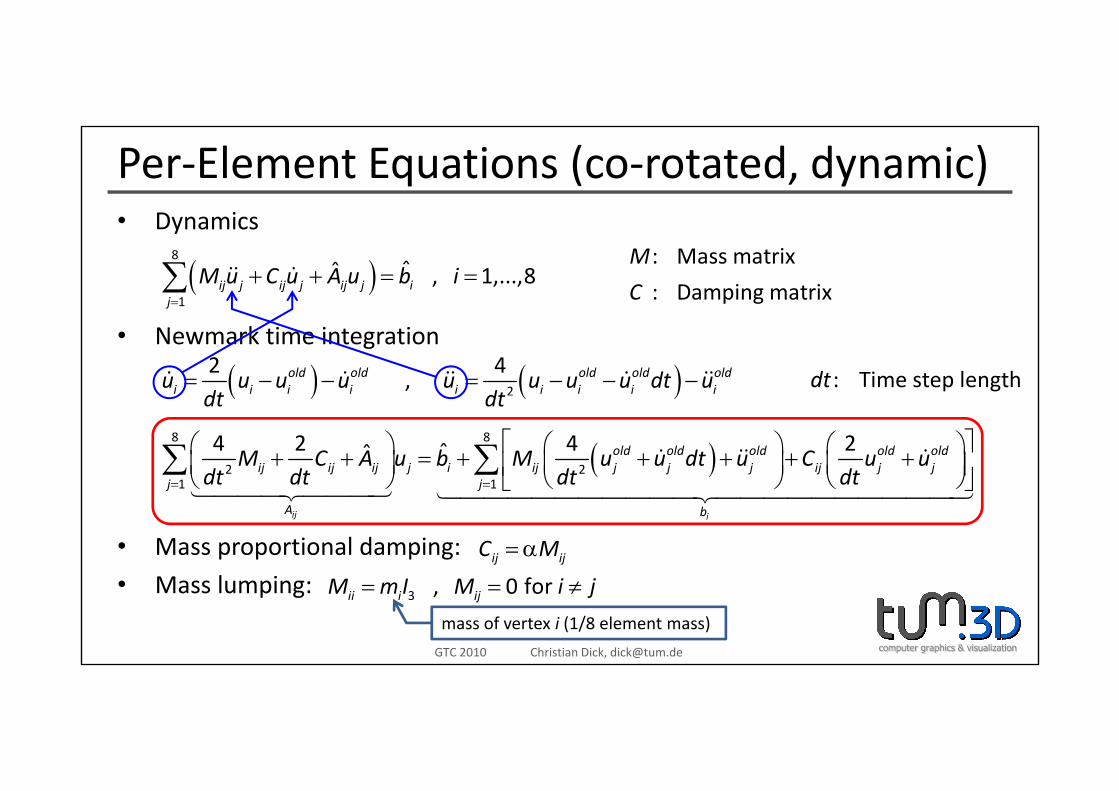
Per‐Element Equations (co‐rotated, dynamic)D i• Dynamics
( )8
1
ˆˆ , 1,...,8=
+ + = =∑ ij j ij j ij j ij
M u C u A u b i: Mass matrix
: Damping matrix
M
C
• Newmark time integration1j
( ) ( )2
2 4,= − − = − − −old old old old old
i i i i i i i i iu u u u u u u u dt udt dt
: Time step lengthdt( ) ( )dt dt
( )8 8
2 21 1
4 2 4 2ˆˆ= =
⎡ ⎤⎛ ⎞ ⎛ ⎞ ⎛ ⎞+ + = + + + + +⎜ ⎟ ⎜ ⎟ ⎜ ⎟⎢ ⎥⎝ ⎠ ⎝ ⎠ ⎝ ⎠⎣ ⎦∑ ∑ old old old old old
ij ij ij j i ij j j j ij j jj j
M C A u b M u u dt u C u udt dt dt dt
• Mass proportional damping:
l
1 1= =⎝ ⎠ ⎝ ⎠ ⎝ ⎠⎣ ⎦ij i
j j
A b
= αij ijC M
computer graphics & visualizationGTC 2010 Christian Dick, [email protected]
• Mass lumping: 3 , 0 for = = ≠ii i ijM m I M i j
mass of vertex i (1/8 element mass)
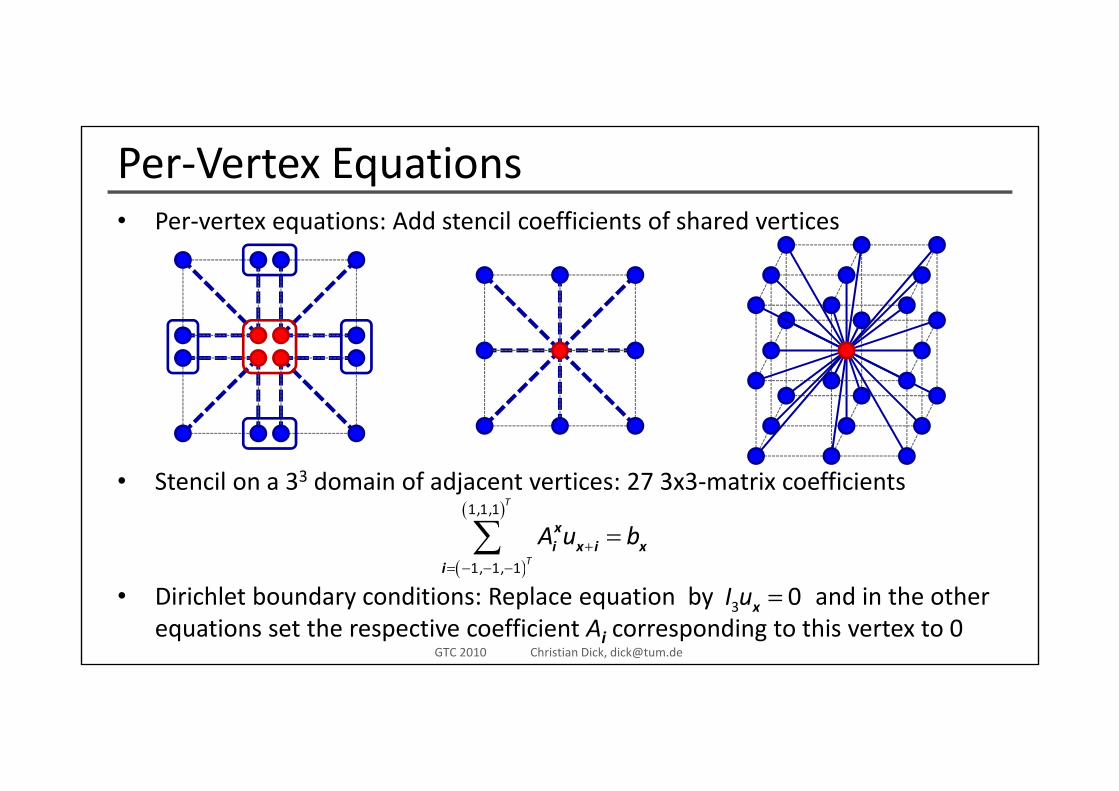
Per‐Vertex EquationsP t ti Add t il ffi i t f h d ti• Per‐vertex equations: Add stencil coefficients of shared vertices
• Stencil on a 33 domain of adjacent vertices: 27 3x3‐matrix coefficientsStencil on a 3 domain of adjacent vertices: 27 3x3 matrix coefficients
( )
( )1,1,1
1, 1, 1
T
T
A u b+= − − −
=∑ xi x i x
i
computer graphics & visualizationGTC 2010 Christian Dick, [email protected]
• Dirichlet boundary conditions: Replace equation by and in the other equations set the respective coefficient Ai corresponding to this vertex to 0
( )
3 0=I ux
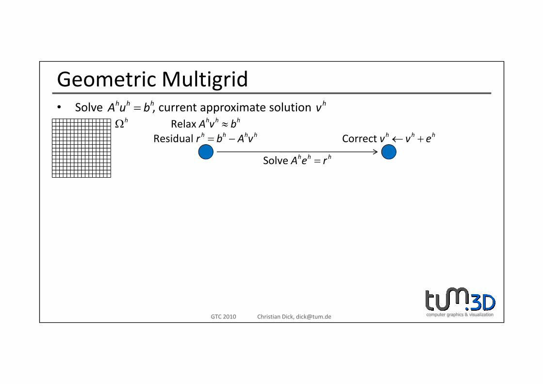
Geometric MultigridS l t i t l tih h hA b h• Solve , current approximate solution=h h hA u b hv
Relax h h hA v b≈Residual h h h hr b A v= − Correct h h hv v e← +
hΩ
Solve h h hA e r=
computer graphics & visualizationGTC 2010 Christian Dick, [email protected]
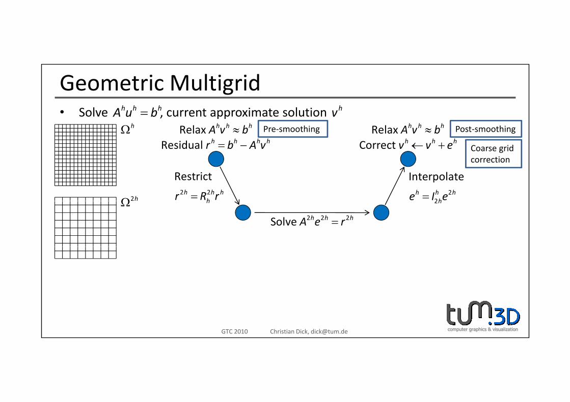
Geometric MultigridS l t i t l tih h hA b h• Solve , current approximate solution=h h hA u b hv
Relax h h hA v b≈Residual h h h hr b A v= −
Relax h h hA v b≈Correct h h hv v e← +
hΩ Pre‐smoothing Post‐smoothing
Coarse grid
2 2
Restricth h h
hr R r= 22
Interpolateh h h
he I e=2hΩ
correction
h 2hΩ2 2 2Solve h h hA e r=
computer graphics & visualizationGTC 2010 Christian Dick, [email protected]
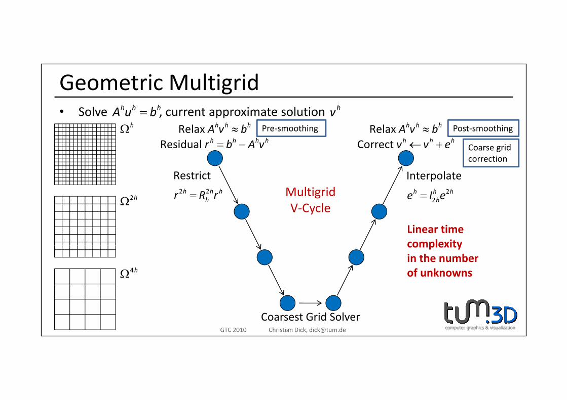
Geometric MultigridS l t i t l tih h hA b h• Solve , current approximate solution=h h hA u b hv
Relax h h hA v b≈Residual h h h hr b A v= −
Relax h h hA v b≈Correct h h hv v e← +
hΩ Pre‐smoothing Post‐smoothing
Coarse grid
2 2
Restricth h h
hr R r= 22
Interpolateh h h
he I e=Multigrid2hΩ
correction
h 2hV‐Cycle
Linear timecomplexity
Ω
complexityin the numberof unknowns4hΩ
computer graphics & visualizationGTC 2010 Christian Dick, [email protected]
Coarsest Grid Solver
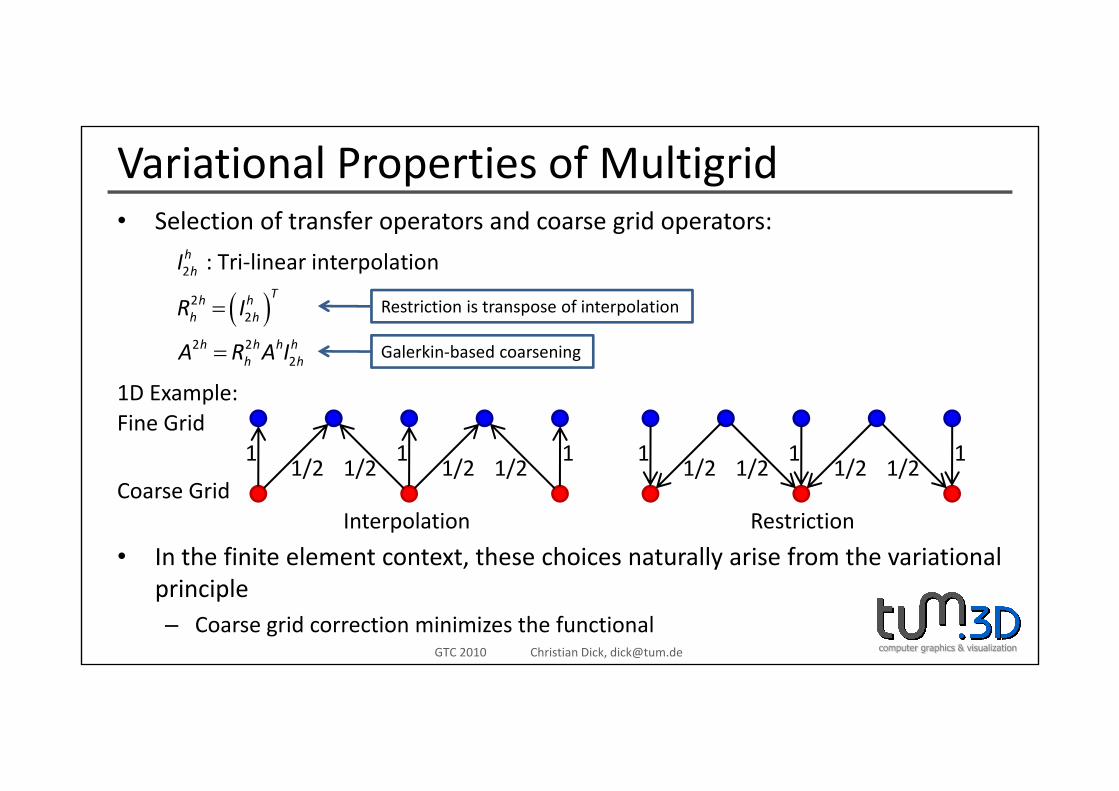
Variational Properties of MultigridS l ti f t f t d id t• Selection of transfer operators and coarse grid operators:
( )2
2
: Tri‐linear interpolationhh
Th h
I
R I Restriction is transpose of interpolation( )2
2 22
h h
h h h hh h
R I
A R A I
=
=
Restriction is transpose of interpolation
Galerkin‐based coarsening
1D Example:
11/2 1/2
11/2 1/2
1Fine Grid
C G id
11/2 1/2
11/2 1/2
1
1D Example:
• In the finite element context, these choices naturally arise from the variational
Coarse GridInterpolation Restriction
computer graphics & visualizationGTC 2010 Christian Dick, [email protected]
principle– Coarse grid correction minimizes the functional
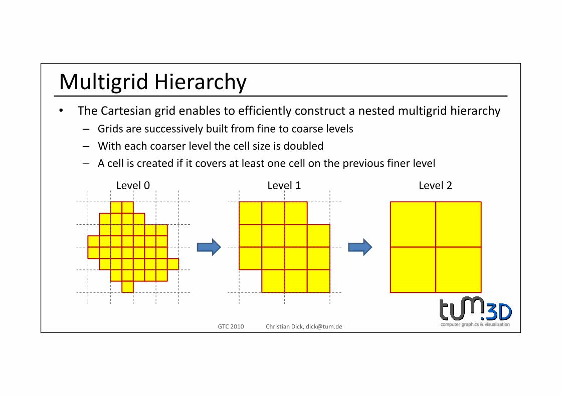
Multigrid HierarchyTh C t i id bl t ffi i tl t t t d lti id hi h• The Cartesian grid enables to efficiently construct a nested multigrid hierarchy– Grids are successively built from fine to coarse levels
– With each coarser level the cell size is doubled
– A cell is created if it covers at least one cell on the previous finer level
Level 0 Level 1 Level 2
computer graphics & visualizationGTC 2010 Christian Dick, [email protected]
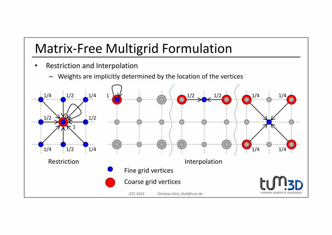
Matrix‐Free Multigrid FormulationR t i ti d I t l ti• Restriction and Interpolation– Weights are implicitly determined by the location of the vertices
1/2 1/2
1/21/4 1/4 1 1/2 1/2 1/4 1/4
1/2 1/2
1
Restriction InterpolationFine grid vertices
1/21/4 1/4 1/4 1/4
computer graphics & visualizationGTC 2010 Christian Dick, [email protected]
Fine grid vertices
Coarse grid vertices
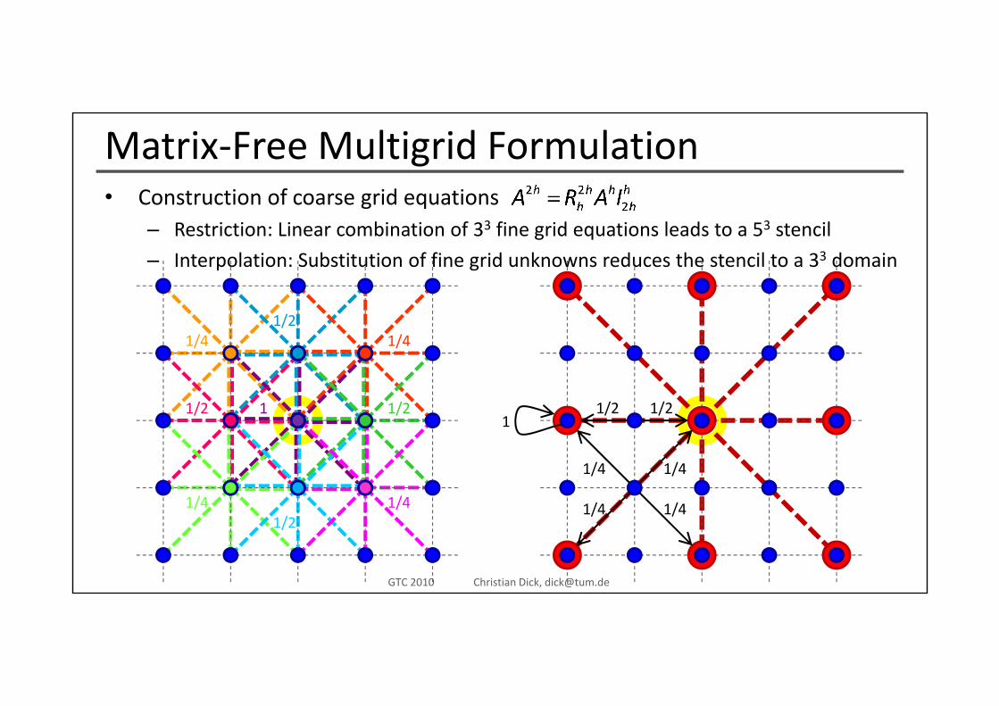
Matrix‐Free Multigrid FormulationC t ti f id ti• Construction of coarse grid equations– Restriction: Linear combination of 33 fine grid equations leads to a 53 stencil
– Interpolation: Substitution of fine grid unknowns reduces the stencil to a 33 domain
1/4 1/41/2
1/2 1/21 1/2 1/21
1/4 1/4
1/4 1/4
1/4 1/4
computer graphics & visualizationGTC 2010 Christian Dick, [email protected]
1/21/4 1/4
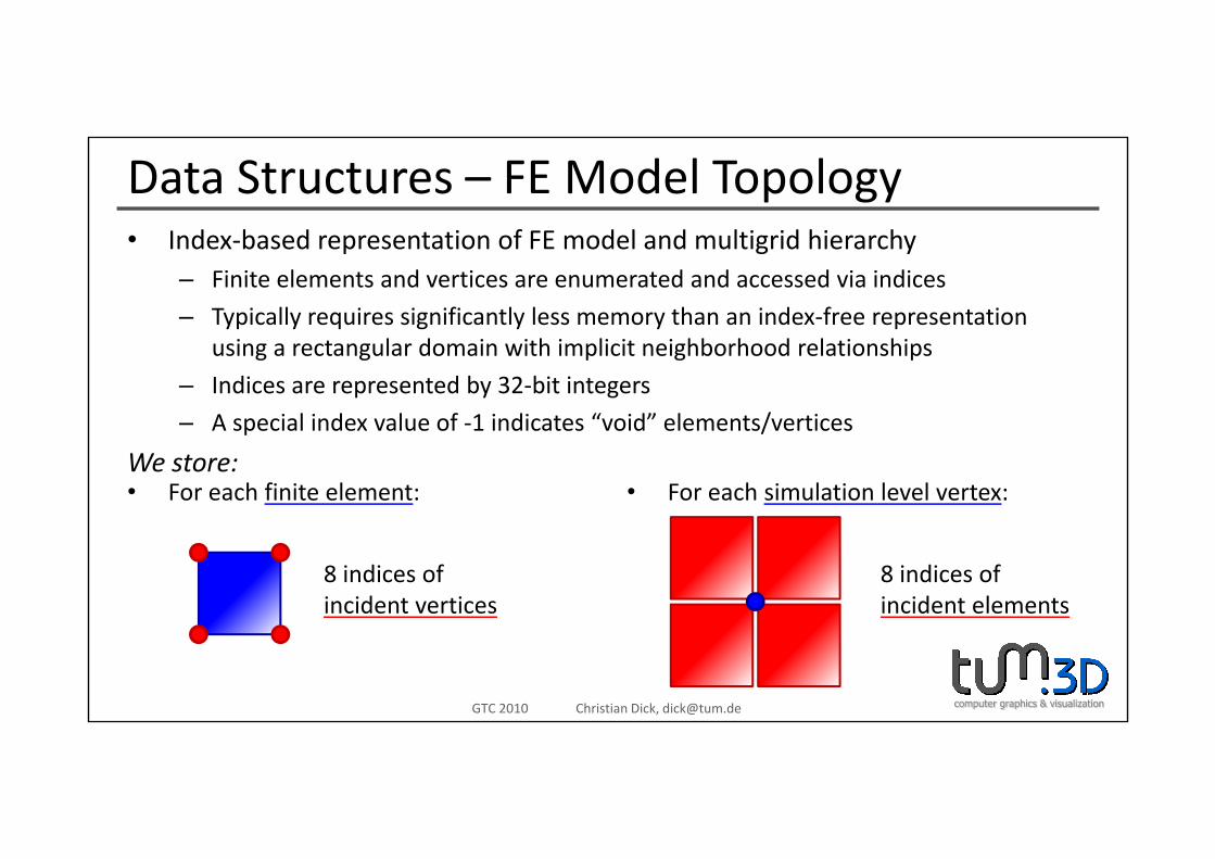
Data Structures – FE Model TopologyI d b d t ti f FE d l d lti id hi h• Index‐based representation of FE model and multigrid hierarchy– Finite elements and vertices are enumerated and accessed via indices
– Typically requires significantly less memory than an index‐free representation using a rectangular domain with implicit neighborhood relationships
– Indices are represented by 32‐bit integers
– A special index value of ‐1 indicates “void” elements/verticesA special index value of 1 indicates void elements/vertices
We store:• For each finite element: • For each simulation level vertex:
8 indices ofincident vertices
8 indices ofincident elements
computer graphics & visualizationGTC 2010 Christian Dick, [email protected]
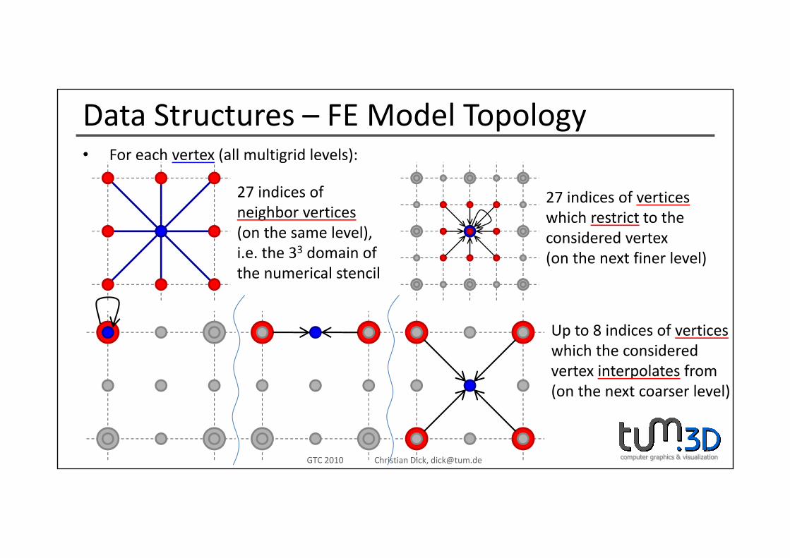
Data Structures – FE Model Topology• For each vertex (all multigrid levels):• For each vertex (all multigrid levels):
27 indices ofneighbor vertices
27 indices of verticeswhich restrict to theneighbor vertices
(on the same level),i.e. the 33 domain ofthe numerical stencil
which restrict to theconsidered vertex(on the next finer level)
Up to 8 indices of verticeswhich the consideredvertex interpolates from(on the next coarser level)
computer graphics & visualizationGTC 2010 Christian Dick, [email protected]
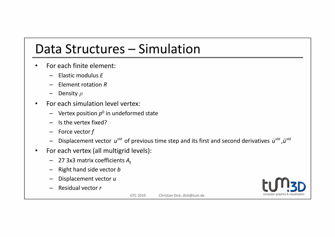
Data Structures – Simulation• For each finite element:• For each finite element:
– Elastic modulus E
– Element rotation RD it– Density ρ
• For each simulation level vertex:– Vertex position p0 in undeformed state
– Is the vertex fixed?
– Force vector f
– Displacement vector of previous time step and its first and second derivatives ,old oldu uoldu
• For each vertex (all multigrid levels):– 27 3x3 matrix coefficients Ai
– Right hand side vector b
computer graphics & visualizationGTC 2010 Christian Dick, [email protected]
g
– Displacement vector u
– Residual vector r
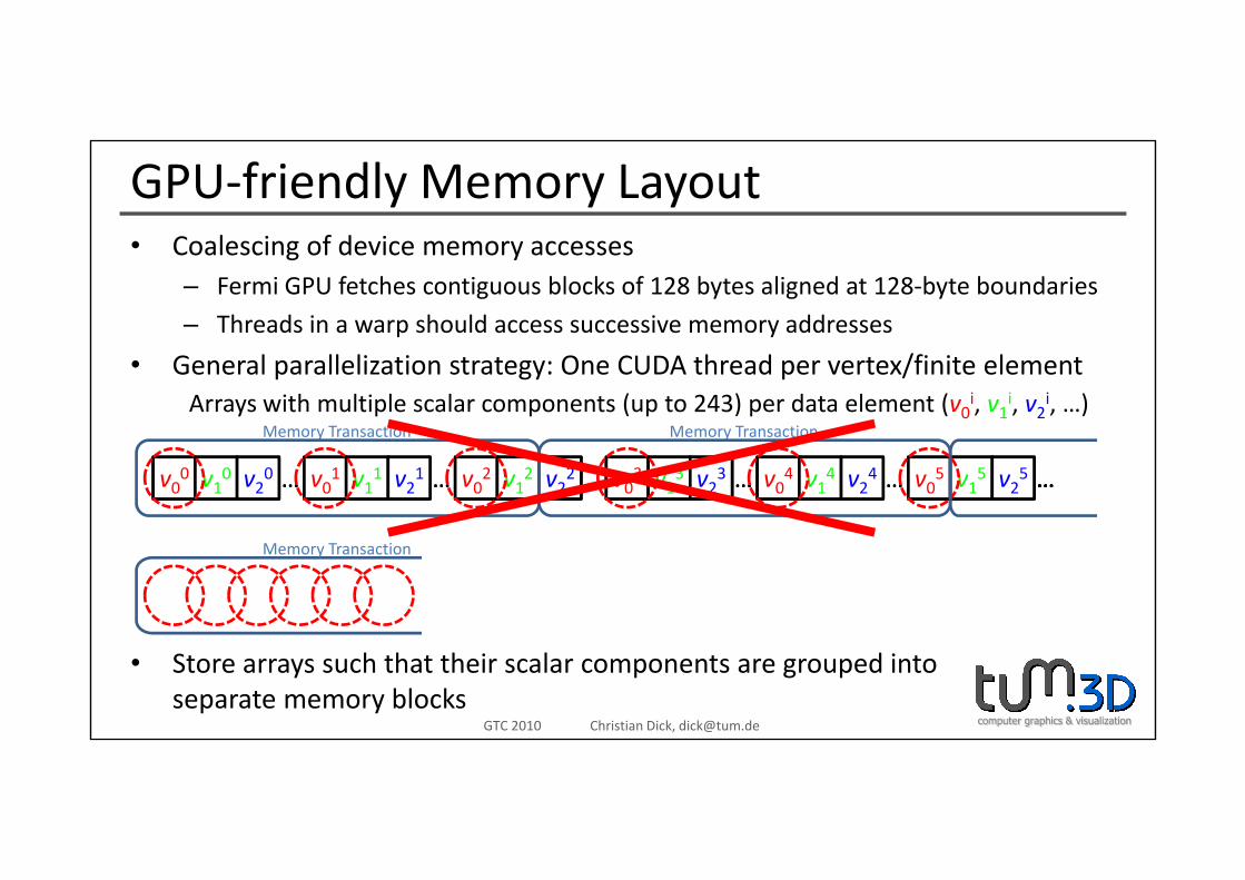
GPU‐friendly Memory LayoutC l i f d i• Coalescing of device memory accesses– Fermi GPU fetches contiguous blocks of 128 bytes aligned at 128‐byte boundaries
– Threads in a warp should access successive memory addresses
• General parallelization strategy: One CUDA thread per vertex/finite elementArrays with multiple scalar components (up to 243) per data element (v0i, v1i, v2i, …)
Memory Transaction Memory Transaction
v00 v10 v20 v01 v11 v21 v02 v12 v22 v03 v13 v23 v04 v14 v24 v05 v15 v25… … … … … …v00 v10 v20 v01 v11 v21 v02 v12 v22 v03 v13 v23 v04 v14 v24 v05 v15 v25… … … … … ………
Memory Transaction
computer graphics & visualizationGTC 2010 Christian Dick, [email protected]
• Store arrays such that their scalar components are grouped intoseparate memory blocks
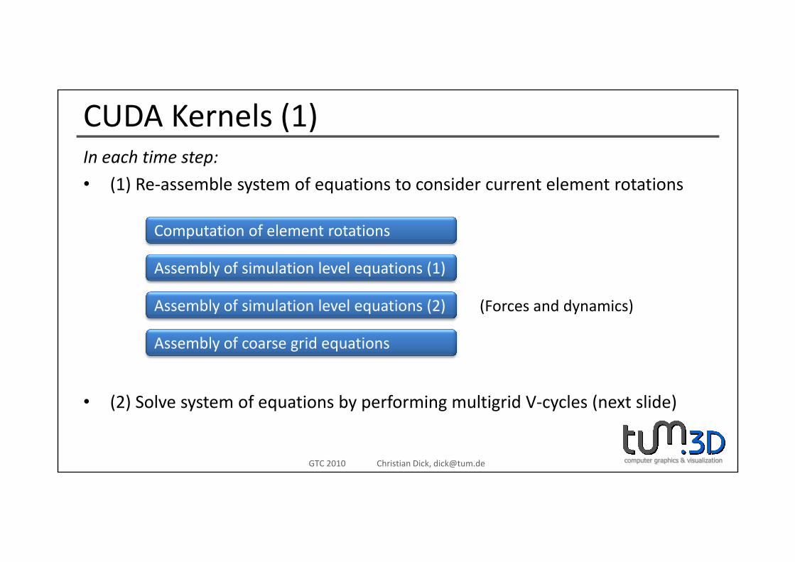
CUDA Kernels (1)I h ti tIn each time step:
• (1) Re‐assemble system of equations to consider current element rotations
Computation of element rotations
Assembly of simulation level equations (1)
Assembly of simulation level equations (2)
Assembly of coarse grid equations
(Forces and dynamics)
• (2) Solve system of equations by performing multigrid V‐cycles (next slide)
Assembly of coarse grid equations
computer graphics & visualizationGTC 2010 Christian Dick, [email protected]
( ) y q y p g g y ( )
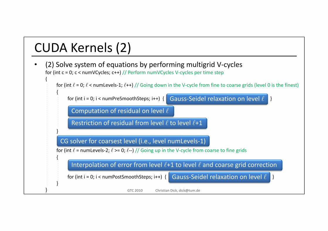
CUDA Kernels (2)(2) S l t f ti b f i lti id V l• (2) Solve system of equations by performing multigrid V‐cycles for (int c = 0; c < numVCycles; c++) // Perform numVCycles V‐cycles per time step{
for (int = 0; < numLevels‐1; ++) // Going down in the V‐cycle from fine to coarse grids (level 0 is the finest){
for (int i = 0; i < numPreSmoothSteps; i++) { }Gauss‐Seidel relaxation on level
Computation of residual on level
}Restriction of residual from level to level +1
CG solver for coarsest level (i e level numLevels‐1)for (int = numLevels‐2; >= 0; ‐‐) // Going up in the V‐cycle from coarse to fine grids{
CG solver for coarsest level (i.e., level numLevels‐1)
Interpolation of error from level +1 to level and coarse grid correction
computer graphics & visualizationGTC 2010 Christian Dick, [email protected]
for (int i = 0; i < numPostSmoothSteps; i++) { } }
}
p g
Gauss‐Seidel relaxation on level
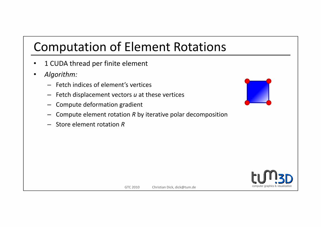
Computation of Element Rotations1 CUDA th d fi it l t• 1 CUDA thread per finite element
• Algorithm:– Fetch indices of element’s vertices
– Fetch displacement vectors u at these vertices
– Compute deformation gradient
Compute element rotation R by iterative polar decomposition– Compute element rotation R by iterative polar decomposition
– Store element rotation R
computer graphics & visualizationGTC 2010 Christian Dick, [email protected]
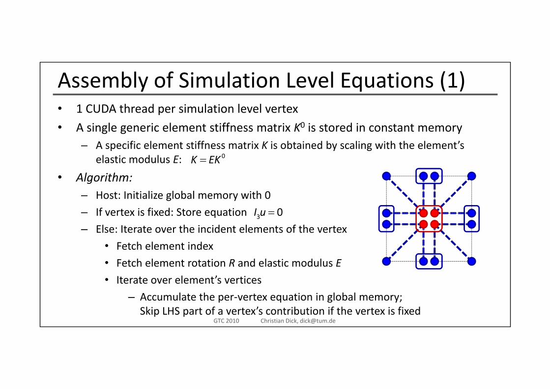
Assembly of Simulation Level Equations (1)1 CUDA th d i l ti l l t• 1 CUDA thread per simulation level vertex
• A single generic element stiffness matrix K0 is stored in constant memory– A specific element stiffness matrix K is obtained by scaling with the element’s p y g
elastic modulus E:
• Algorithm:Host: Initialize global memory with 0
0K EK=
– Host: Initialize global memory with 0
– If vertex is fixed: Store equation
– Else: Iterate over the incident elements of the vertex3 0I u =
• Fetch element index
• Fetch element rotation R and elastic modulus E
• Iterate over element’s vertices
computer graphics & visualizationGTC 2010 Christian Dick, [email protected]
Iterate over element s vertices
– Accumulate the per‐vertex equation in global memory;Skip LHS part of a vertex’s contribution if the vertex is fixed
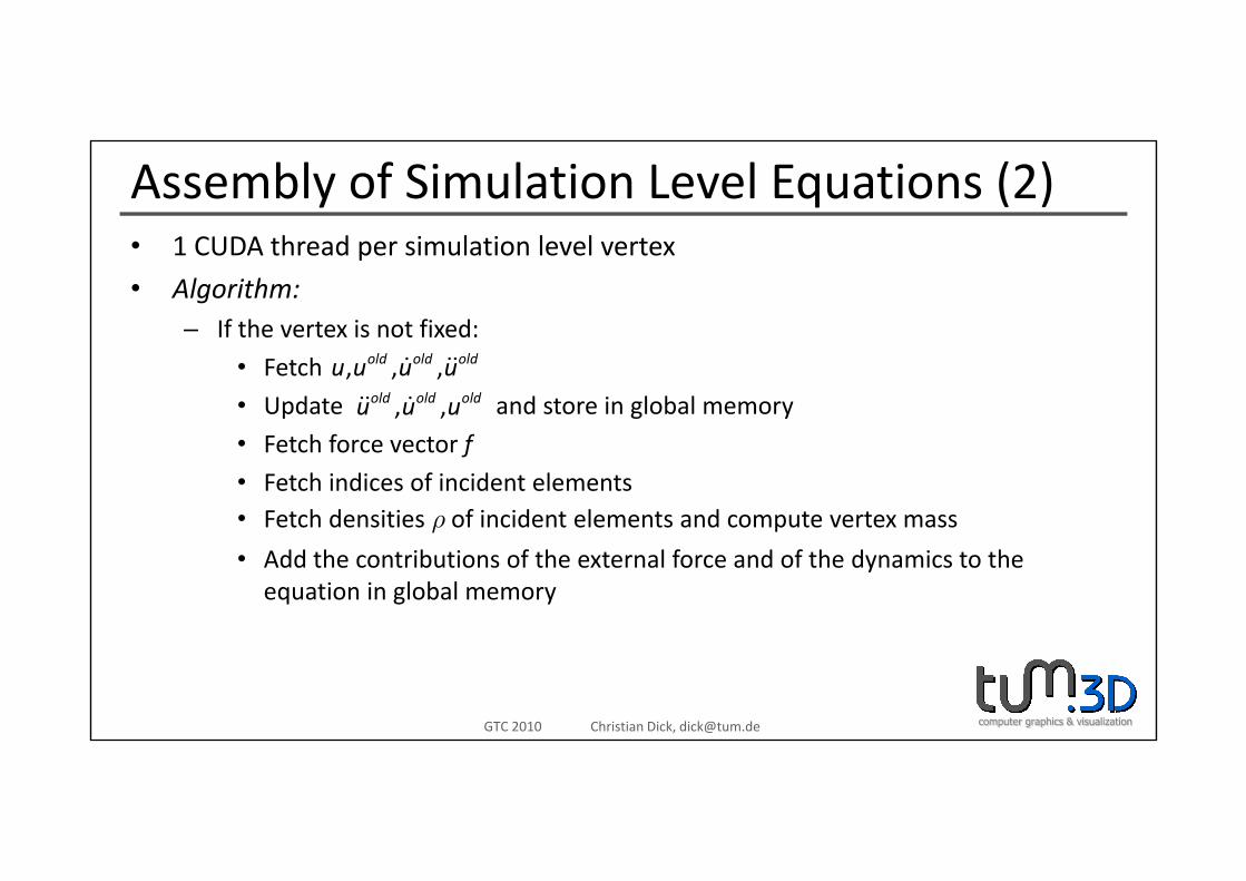
Assembly of Simulation Level Equations (2)1 CUDA th d i l ti l l t• 1 CUDA thread per simulation level vertex
• Algorithm:– If the vertex is not fixed:
• Fetch
• Update and store in global memory
• Fetch force vector f
, , ,old old oldu u u u
, ,old old oldu u u• Fetch force vector f
• Fetch indices of incident elements• Fetch densities ρ of incident elements and compute vertex mass
• Add the contributions of the external force and of the dynamics to the equation in global memory
computer graphics & visualizationGTC 2010 Christian Dick, [email protected]
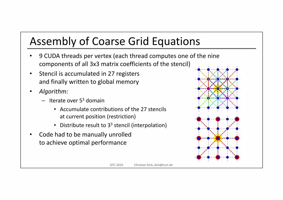
Assembly of Coarse Grid Equations9 CUDA th d t ( h th d t f th i• 9 CUDA threads per vertex (each thread computes one of the nine components of all 3x3 matrix coefficients of the stencil)
• Stencil is accumulated in 27 registersand finally written to global memory
• Algorithm:Iterate over 53 domain– Iterate over 53 domain
• Accumulate contributions of the 27 stencilsat current position (restriction)
3• Distribute result to 33 stencil (interpolation)
• Code had to be manually unrolledto achieve optimal performance
computer graphics & visualizationGTC 2010 Christian Dick, [email protected]
p p
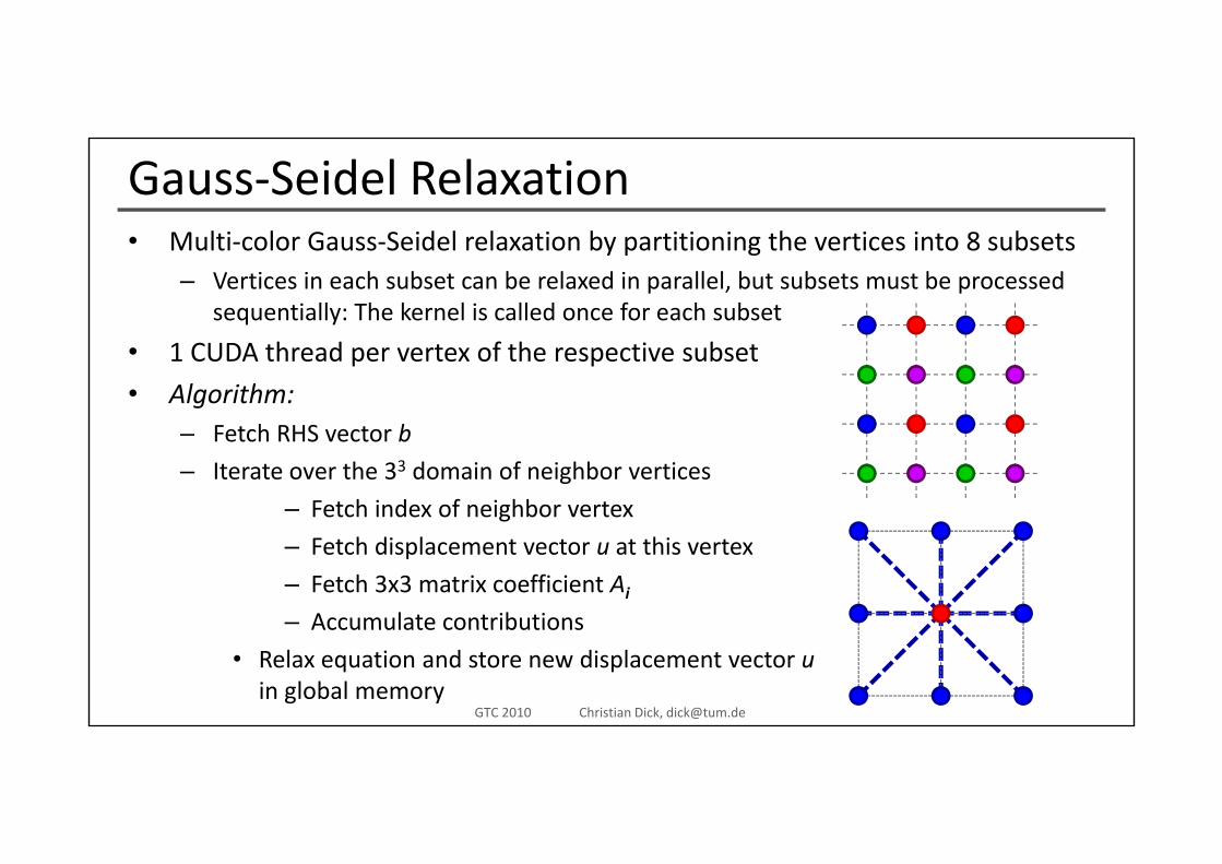
Gauss‐Seidel RelaxationM lti l G S id l l ti b titi i th ti i t 8 b t• Multi‐color Gauss‐Seidel relaxation by partitioning the vertices into 8 subsets– Vertices in each subset can be relaxed in parallel, but subsets must be processed
sequentially: The kernel is called once for each subset
• 1 CUDA thread per vertex of the respective subset
• Algorithm:Fetch RHS vector b– Fetch RHS vector b
– Iterate over the 33 domain of neighbor vertices
– Fetch index of neighbor vertex
– Fetch displacement vector u at this vertex
– Fetch 3x3 matrix coefficient Ai
– Accumulate contributions
computer graphics & visualizationGTC 2010 Christian Dick, [email protected]
Accumulate contributions
• Relax equation and store new displacement vector uin global memory
Computation of Residual1 CUDA th d t• 1 CUDA thread per vertex
• Similar to Gauss‐Seidel relaxation, however now all vertices can be processed in parallel with a single kernel call
computer graphics & visualizationGTC 2010 Christian Dick, [email protected]
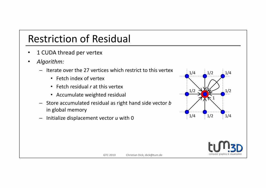
Restriction of Residual1 CUDA th d t• 1 CUDA thread per vertex
• Algorithm:– Iterate over the 27 vertices which restrict to this vertex 1/21/4 1/4
• Fetch index of vertex
• Fetch residual r at this vertex
• Accumulate weighted residual1/2 1/2
1/21/4 1/4
• Accumulate weighted residual
– Store accumulated residual as right hand side vector bin global memory
1/21/4 1/4
1
– Initialize displacement vector u with 0 1/21/4 1/4
computer graphics & visualizationGTC 2010 Christian Dick, [email protected]
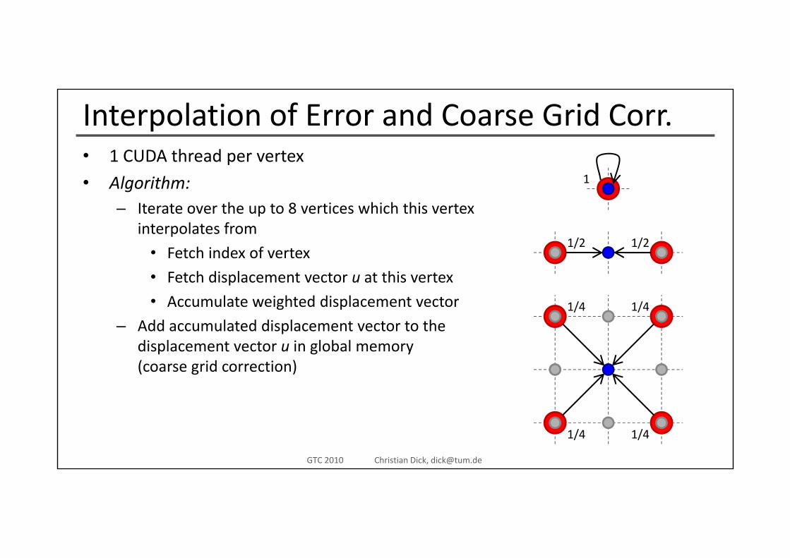
Interpolation of Error and Coarse Grid Corr.1 CUDA th d t• 1 CUDA thread per vertex
• Algorithm:– Iterate over the up to 8 vertices which this vertex
1
pinterpolates from
• Fetch index of vertex
• Fetch displacement vector u at this vertex
1/2 1/2
Fetch displacement vector u at this vertex
• Accumulate weighted displacement vector
– Add accumulated displacement vector to thedi l t t i l b l
1/4 1/4
displacement vector u in global memory(coarse grid correction)
computer graphics & visualizationGTC 2010 Christian Dick, [email protected]
1/4 1/4
Solver for the Coarsest LevelC j t di t (CG) l ith J bi diti (i di l)• Conjugate gradient (CG) solver with Jacobi pre‐conditioner (inverse diagonal)
• Runs on a single multiprocessor (using a single thread block) to avoid global synchronization via separate kernel calls
• 1 CUDA thread per vertex
• Number of unknowns is limited by the maximum number of threads per block and by the size of the shared memoryand by the size of the shared memory– Number of multigrid levels is chosen such that the number of vertices
on the coarsest grid is ≤ 512
computer graphics & visualizationGTC 2010 Christian Dick, [email protected]
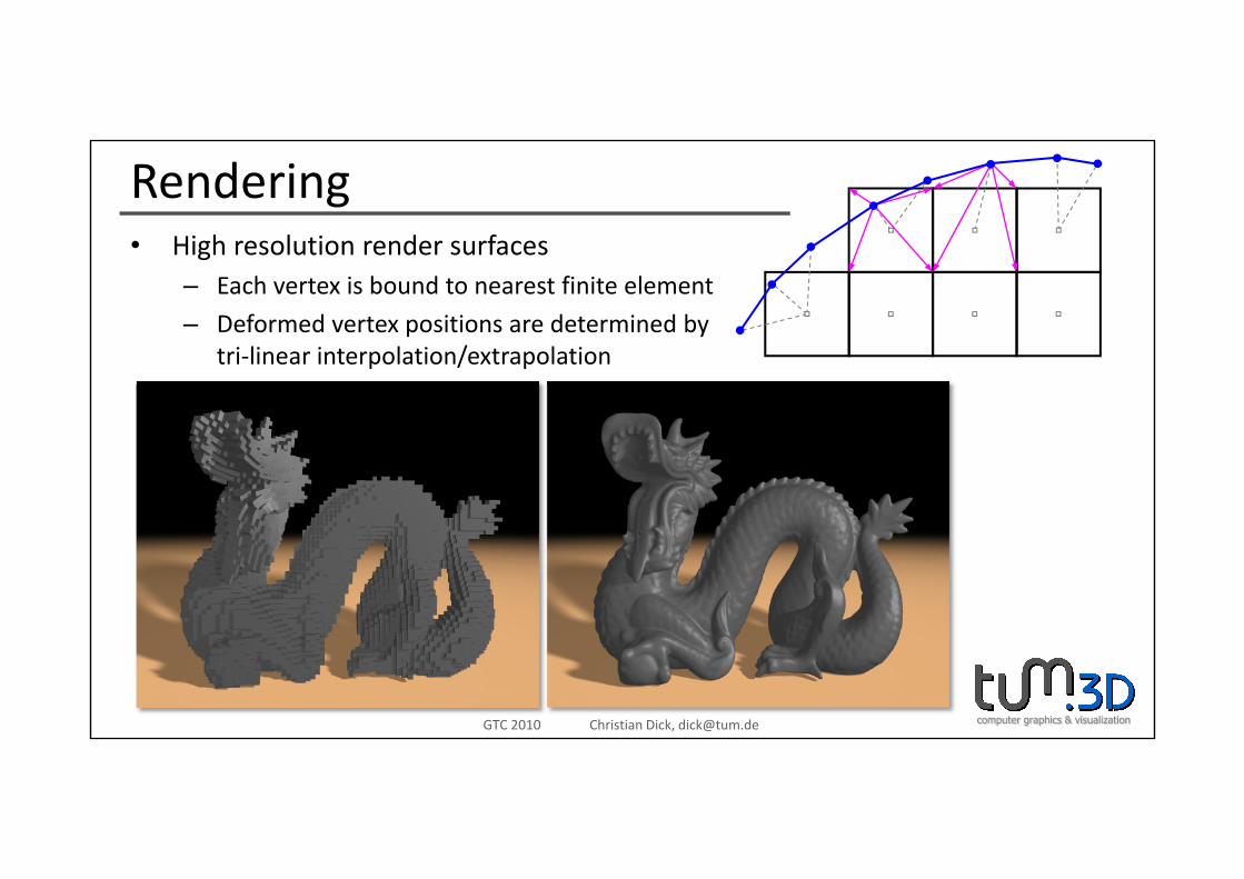
RenderingHi h l ti d f• High resolution render surfaces– Each vertex is bound to nearest finite element
– Deformed vertex positions are determined bytri‐linear interpolation/extrapolation
computer graphics & visualizationGTC 2010 Christian Dick, [email protected]
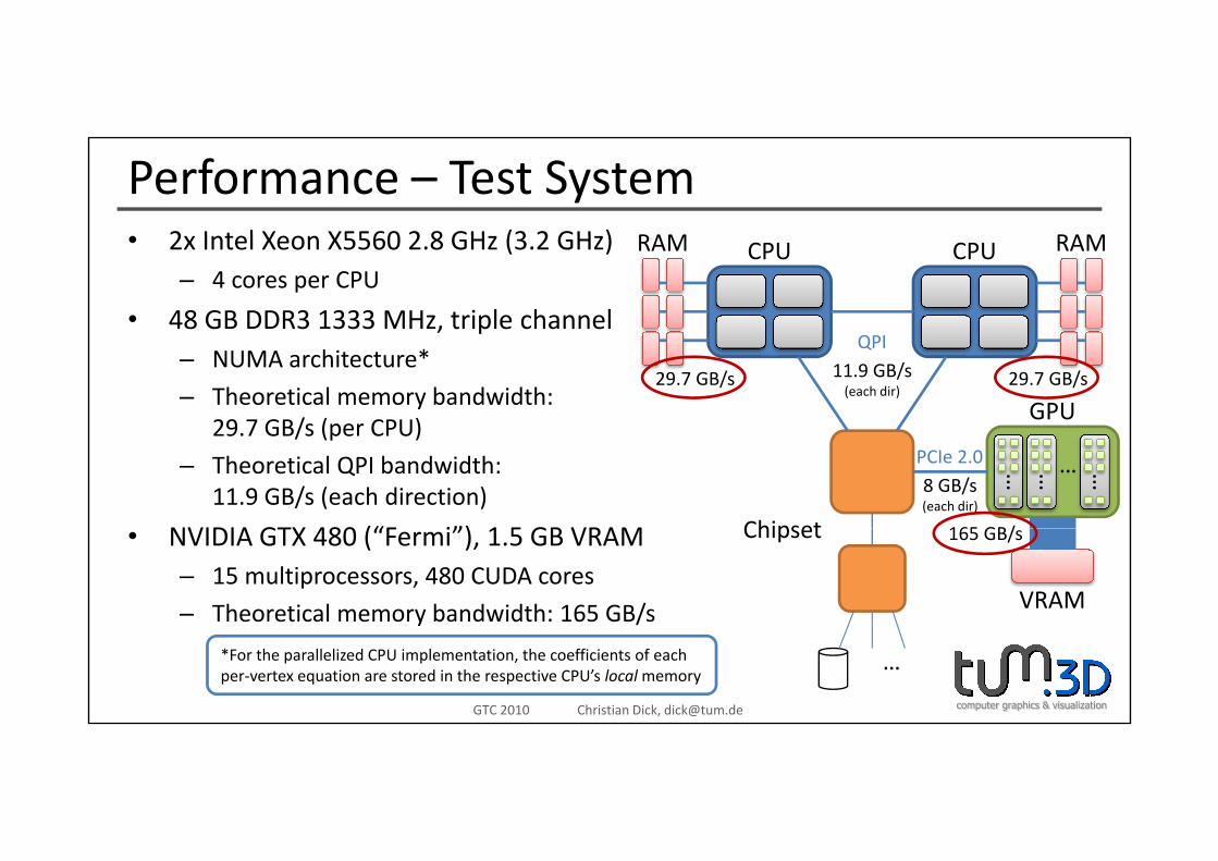
Performance – Test System2 I t l X X5560 2 8 GH (3 2 GH ) RAM RAM• 2x Intel Xeon X5560 2.8 GHz (3.2 GHz)– 4 cores per CPU
• 48 GB DDR3 1333 MHz, triple channel
CPU CPURAM RAM
, p– NUMA architecture*
– Theoretical memory bandwidth:29 7 GB/s (per CPU)
QPI11.9 GB/s(each dir)
29.7 GB/s 29.7 GB/s
GPU29.7 GB/s (per CPU)
– Theoretical QPI bandwidth:11.9 GB/s (each direction)
NVIDIA GTX 480 (“F i”) 1 5 GB VRAM Chipset
PCIe 2.0
165 GB/
8 GB/s(each dir)
… … …
…
• NVIDIA GTX 480 (“Fermi”), 1.5 GB VRAM– 15 multiprocessors, 480 CUDA cores
– Theoretical memory bandwidth: 165 GB/s
Chipset
VRAM
165 GB/s
computer graphics & visualizationGTC 2010 Christian Dick, [email protected]
…*For the parallelized CPU implementation, the coefficients of eachper‐vertex equation are stored in the respective CPU’s localmemory
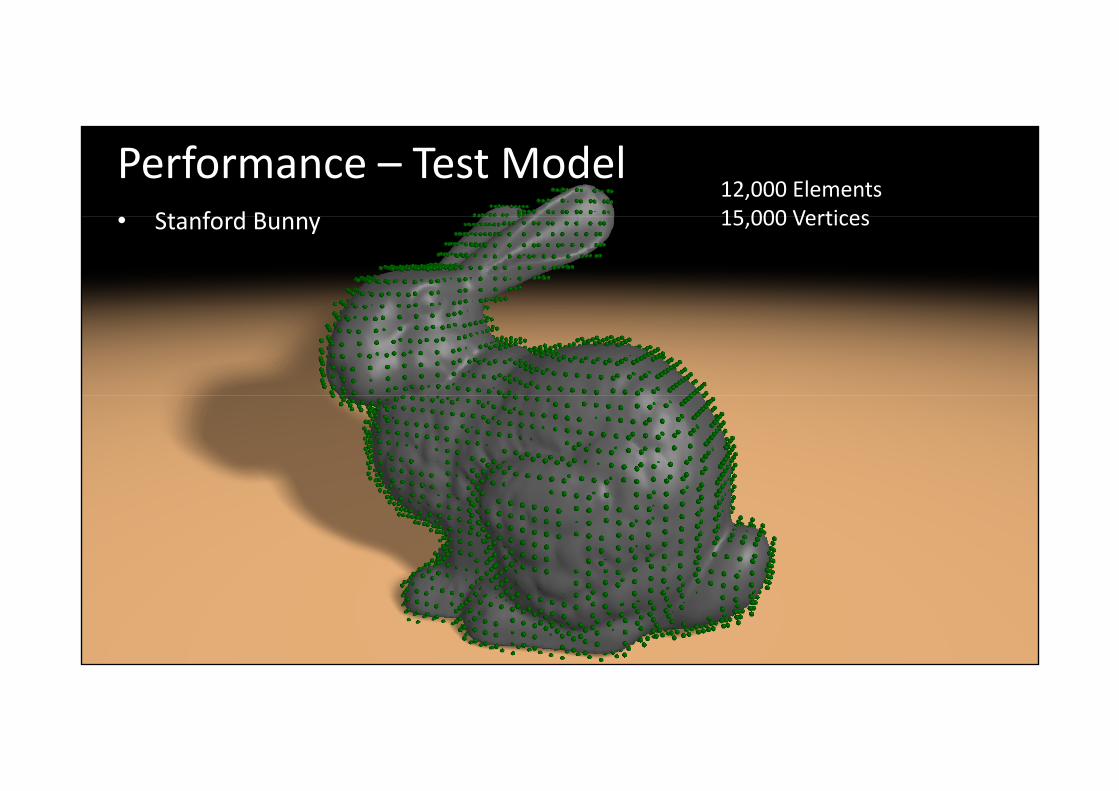
Performance – Test ModelSt f d B
12,000 Elements15 000 Vertices• Stanford Bunny 15,000 Vertices
computer graphics & visualizationGTC 2010 Christian Dick, [email protected]

Performance – Test ModelSt f d B
33,000 Elements39 000 Vertices• Stanford Bunny 39,000 Vertices
computer graphics & visualizationGTC 2010 Christian Dick, [email protected]
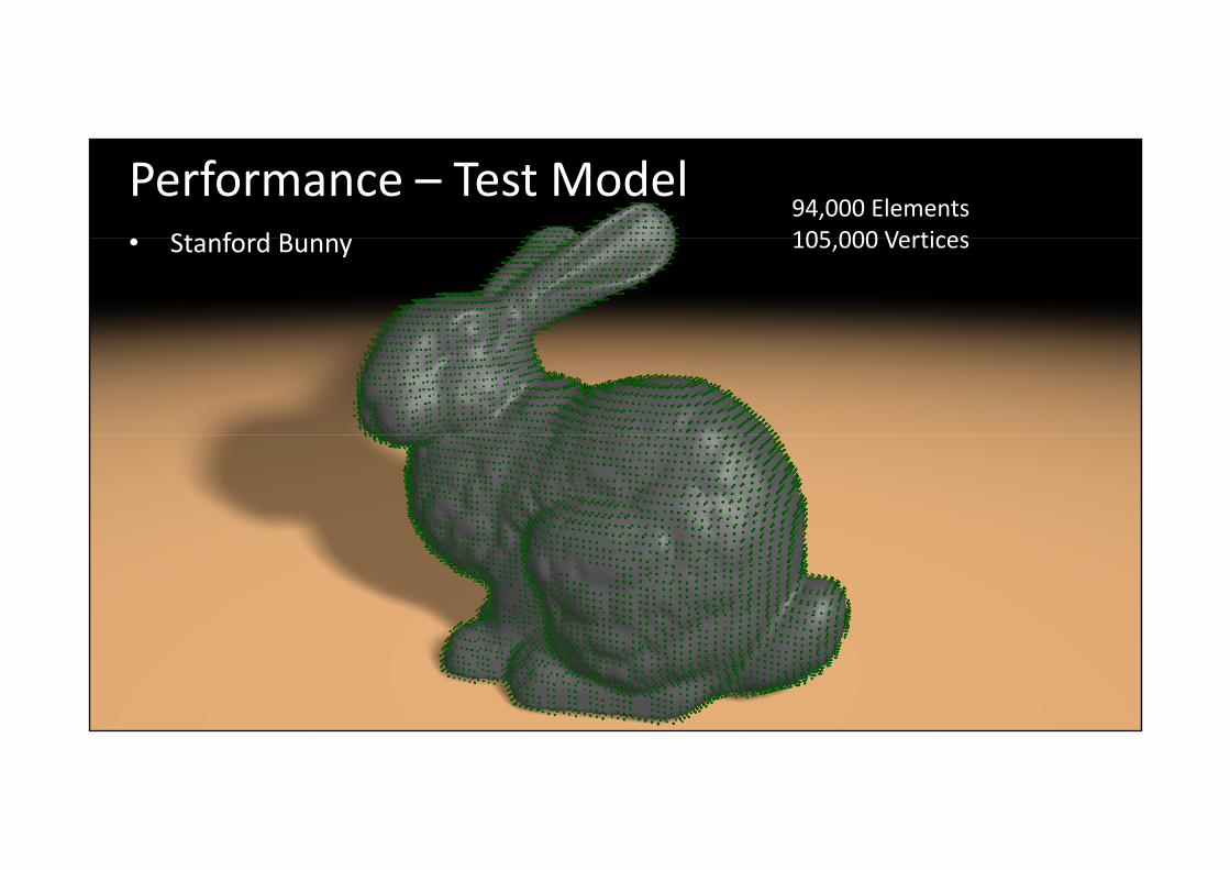
Performance – Test ModelSt f d B
94,000 Elements105 000 Vertices• Stanford Bunny 105,000 Vertices
computer graphics & visualizationGTC 2010 Christian Dick, [email protected]

Performance – Test ModelSt f d B
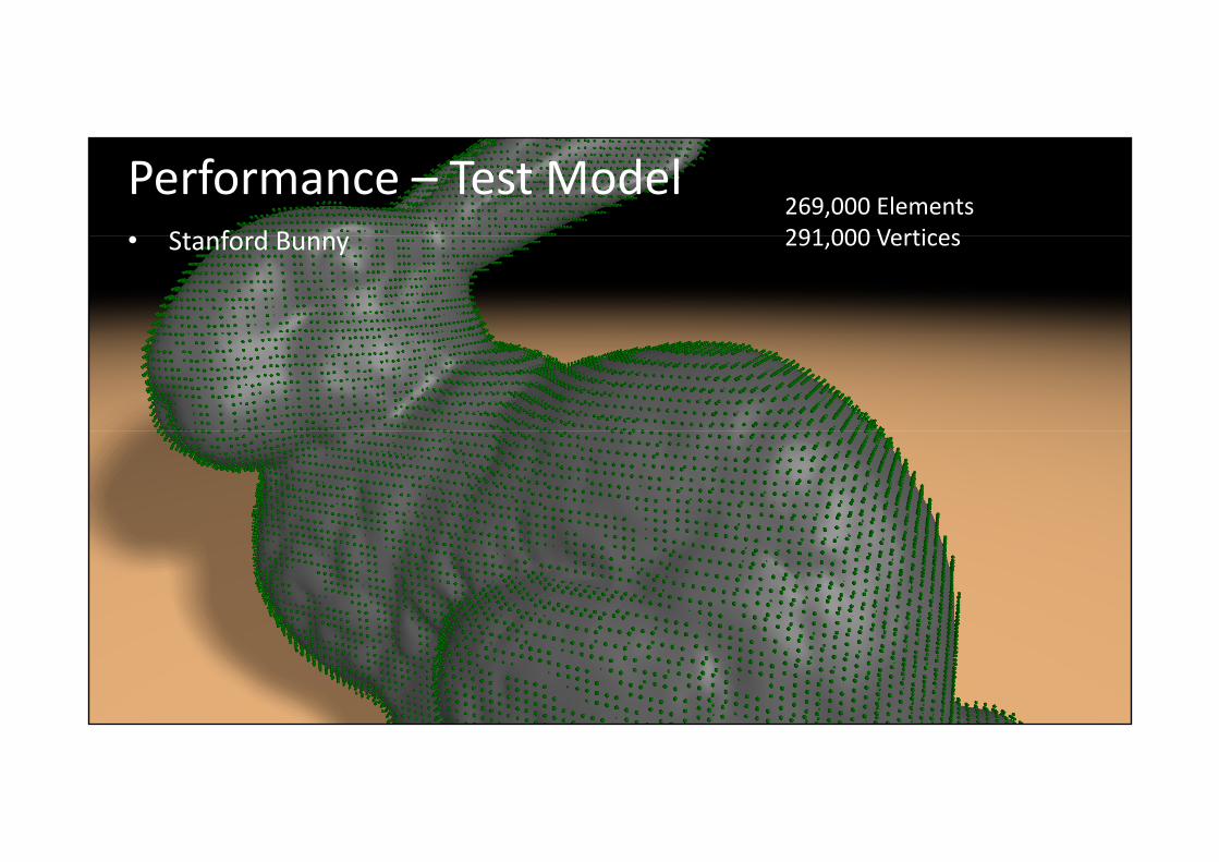
269,000 Elements291 000 Vertices• Stanford Bunny 291,000 Vertices
computer graphics & visualizationGTC 2010 Christian Dick, [email protected]
Performance – Test ModelSt f d B
269,000 Elements291 000 Vertices• Stanford Bunny 291,000 Vertices
computer graphics & visualizationGTC 2010 Christian Dick, [email protected]
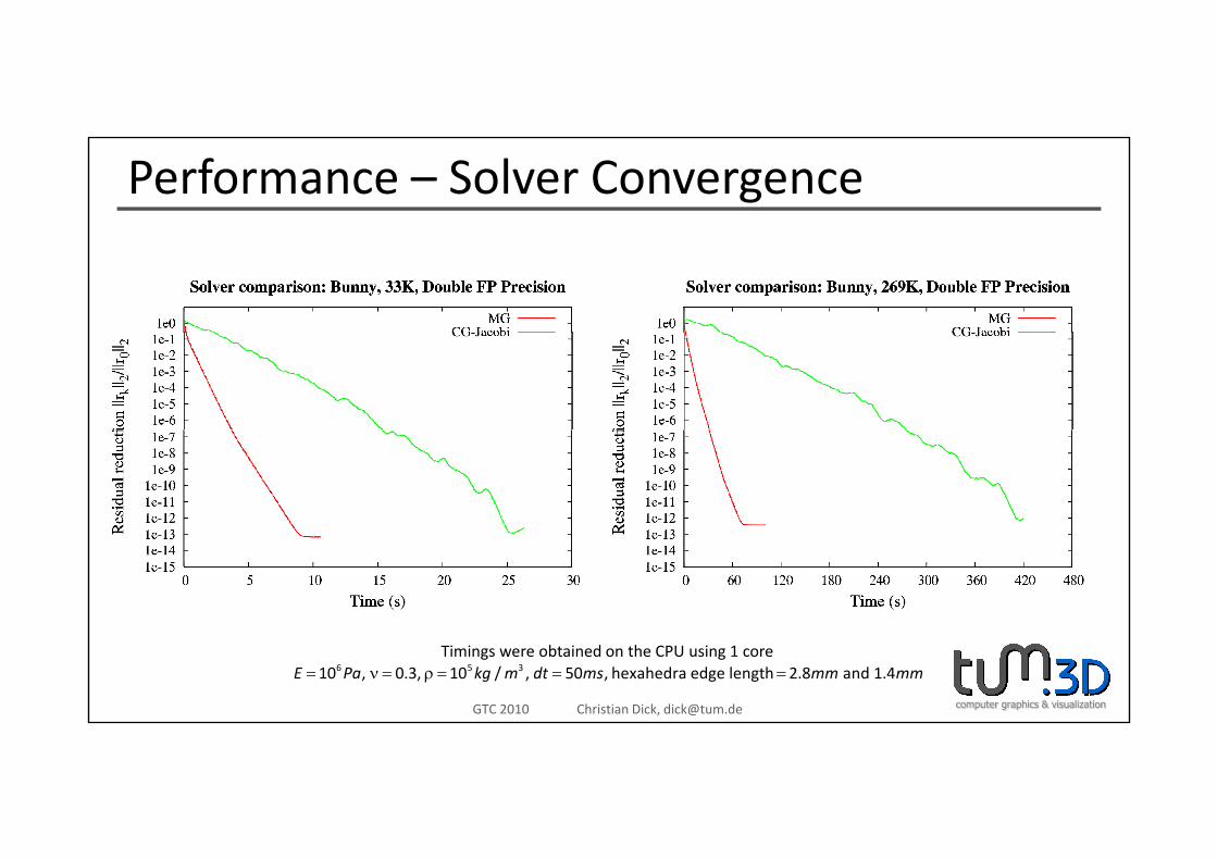
Performance – Solver Convergence
computer graphics & visualizationGTC 2010 Christian Dick, [email protected]
6 5 310 , 0.3, 10 / , 50 , hexahedra edge length 2.8 and 1.4E Pa kg m dt ms mm mm= ν = ρ = = =Timings were obtained on the CPU using 1 core
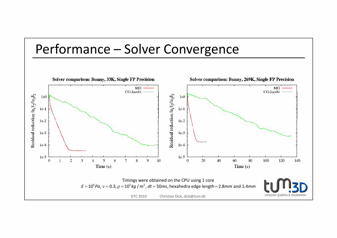
Performance – Solver Convergence
computer graphics & visualizationGTC 2010 Christian Dick, [email protected]
6 5 310 , 0.3, 10 / , 50 , hexahedra edge length 2.8 and 1.4E Pa kg m dt ms mm mm= ν = ρ = = =Timings were obtained on the CPU using 1 core
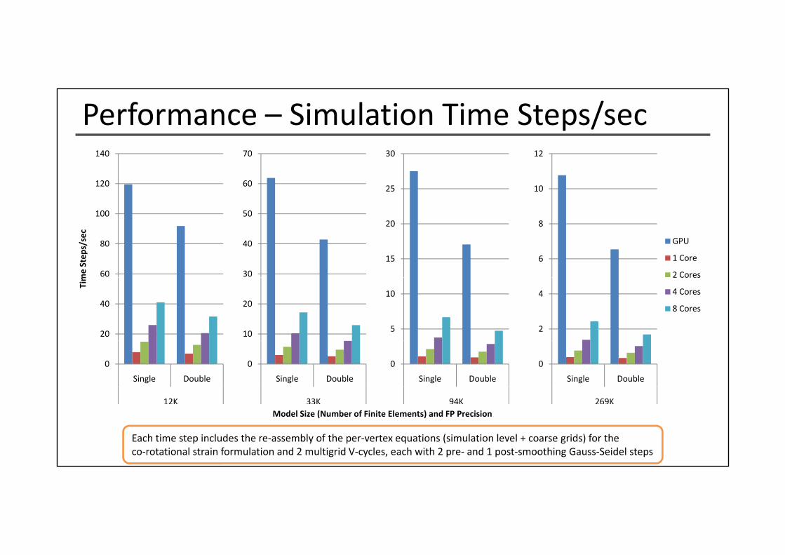
Performance – Simulation Time Steps/sec140 70 30 12
100
120
140
50
60
70
25
30
10
12
60
80
100
me Step
s/sec
30
40
50
15
20
6
8
GPU
1 Core
2 Cores
20
40
Tim
10
20
5
10
2
4
2 Cores
4 Cores
8 Cores
0
Single Double
12K
0
Single Double
33K
0
Single Double
94K
0
Single Double
269K
computer graphics & visualizationGTC 2010 Christian Dick, [email protected]
12K 33K 94K 269KModel Size (Number of Finite Elements) and FP Precision
Each time step includes the re‐assembly of the per‐vertex equations (simulation level + coarse grids) for theco‐rotational strain formulation and 2 multigrid V‐cycles, each with 2 pre‐ and 1 post‐smoothing Gauss‐Seidel steps
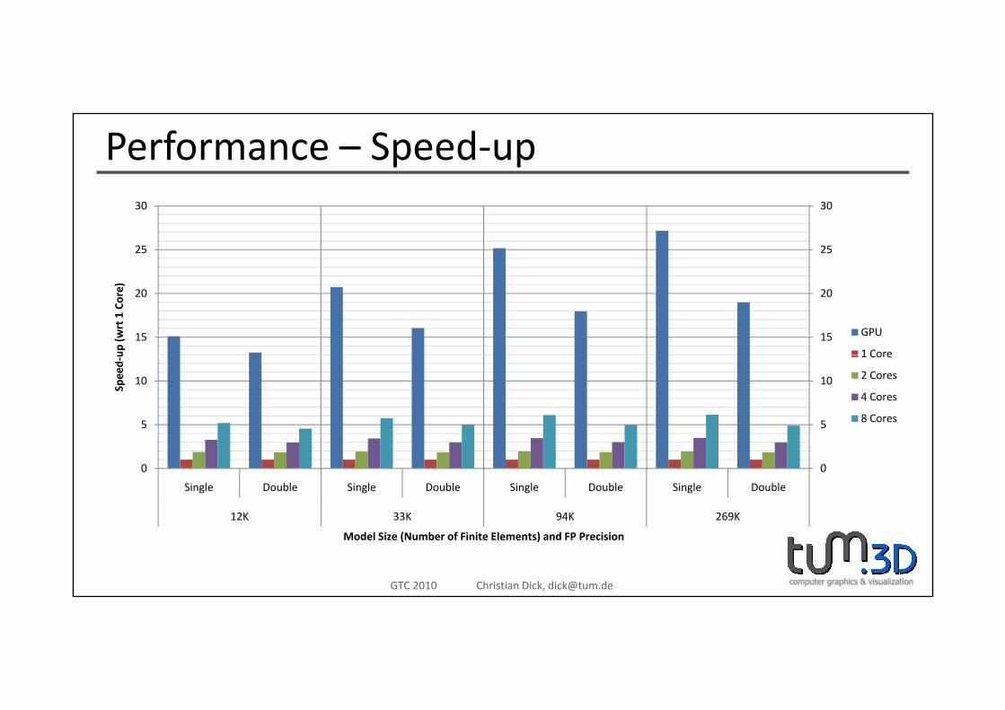
Performance – Speed‐up
25
30
25
30
15
20
15
20
up (w
rt 1 Core)
GPU
1 Core
5
10
5
10
Speed‐u 1 Core
2 Cores
4 Cores
8 Cores
00
Single Double Single Double Single Double Single Double
12K 33K 94K 269K
computer graphics & visualizationGTC 2010 Christian Dick, [email protected]
12K 33K 94K 269K
Model Size (Number of Finite Elements) and FP Precision
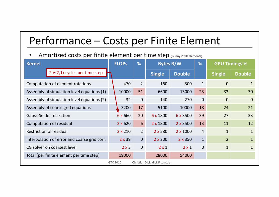
Performance – Costs per Finite ElementA ti d t fi it l t ti t• Amortized costs per finite element per time step (Bunny 269K elements)
Kernel FLOPs % Bytes R/W % GPU Timings %
Single Double Single Double2 V(2,1)‐cycles per time step g g
Computation of element rotations 470 2 160 300 1 0 1
Assembly of simulation level equations (1) 10000 51 6600 13000 23 33 30
A bl f i l ti l l ti (2) 32 0 140 270 0 0 0Assembly of simulation level equations (2) 32 0 140 270 0 0 0
Assembly of coarse grid equations 3200 17 5100 10000 18 24 21
Gauss‐Seidel relaxation 6 x 660 20 6 x 1800 6 x 3500 39 27 33
Computation of residual 2 x 620 6 2 x 1800 2 x 3500 13 11 12
Restriction of residual 2 x 210 2 2 x 580 2 x 1000 4 1 1
Interpolation of error and coarse grid corr. 2 x 39 0 2 x 200 2 x 350 1 2 1
computer graphics & visualizationGTC 2010 Christian Dick, [email protected]
CG solver on coarsest level 2 x 3 0 2 x 1 2 x 1 0 1 1
Total (per finite element per time step) 19000 28000 54000
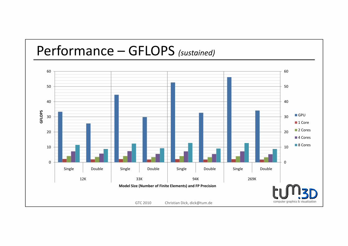
Performance – GFLOPS (sustained)
50
60
50
60
30
40
30
40
GFLOPS GPU
1 Core
10
20
10
20
G 1 Core
2 Cores
4 Cores
8 Cores
00
Single Double Single Double Single Double Single Double
12K 33K 94K 269K
computer graphics & visualizationGTC 2010 Christian Dick, [email protected]
12K 33K 94K 269K
Model Size (Number of Finite Elements) and FP Precision
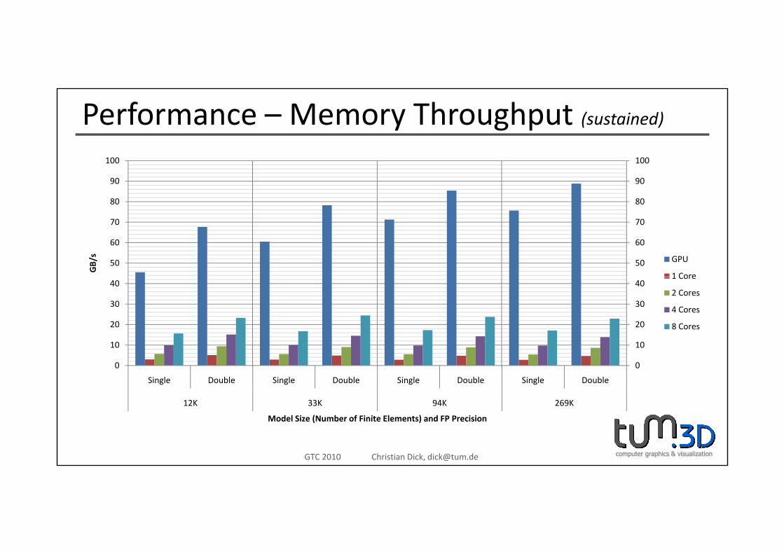
Performance – Memory Throughput (sustained)
80
90
100
80
90
100
50
60
70
50
60
70
GB/s GPU
1 Core
20
30
40
20
30
401 Core
2 Cores
4 Cores
8 Cores
0
10
0
10
Single Double Single Double Single Double Single Double
12K 33K 94K 269K
computer graphics & visualizationGTC 2010 Christian Dick, [email protected]
12K 33K 94K 269K
Model Size (Number of Finite Elements) and FP Precision
Conclusion and Future WorkR l ti FEM i l ti f d f bl bj t bl d b• Real‐time FEM simulation of deformable objects enabled by afully GPU‐based geometric multigrid solver– Hexahedral finite elements on a uniform Cartesian grid, co‐rotational strain
– Regular shape of stencil enables GPU‐friendly parallelization and memory accesses
– Performance is boosted by the GPU’s compute power and memory bandwidth
• Up to 27x faster than 1 CPU core / 4x faster than 8 CPU coresUp to 27x faster than 1 CPU core / 4x faster than 8 CPU cores
• Up to 56 GFLOPS (single) / 34 GFLOPS (double precision) (sustained performance)
• Up to 88 GB/s memory throughput (sustained performance)
• Real‐time/interactive simulation rates:120 time steps/sec for 12,000 elements, 11 time steps/sec for 269,000 elements
• Future work
computer graphics & visualizationGTC 2010 Christian Dick, [email protected]
– GPU‐based collision detection
– Parallelization on multiple GPUs
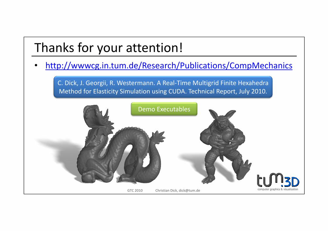
Thanks for your attention!htt // i t d /R h/P bli ti /C M h i• http://wwwcg.in.tum.de/Research/Publications/CompMechanics
C. Dick, J. Georgii, R. Westermann. A Real‐Time Multigrid Finite Hexahedra M h d f El i i Si l i i CUDA T h i l R J l 2010Method for Elasticity Simulation using CUDA. Technical Report, July 2010.
Demo Executables
computer graphics & visualizationGTC 2010 Christian Dick, [email protected]