1

Data matching (or Duplicate Detection or Record Linkage)

Helena Galhardas DEI IST

References

n  Chapter 7 (Sects. 7.1, 7.2, 7.3, 7.7), “Principles of Data Integration” by AnHai Doan, Alon Halevy, Zachary Ives, 2012.

n  Slides “Data Quality and Data Cleansing” course, Felix Naumann, Winter 2014/15

n  “Data Matching”, Peter Christen, Springer. n  “An Introduction to Duplicate Detection”, F. Naumann

and Melanie Herschel, Morgan Claypool Publishers. n  “The Merge/Purge Problem for Large Databases”, M.

Hernandez and S. Stolfo, SIGMOD 1995. n  “Real-world Data is Dirty: Data Cleansing and The

Merge/Purge Problem”, M. Hernandez and S. Stolfo, Data Mining and Knowledge Discovery, 1998.

2

2

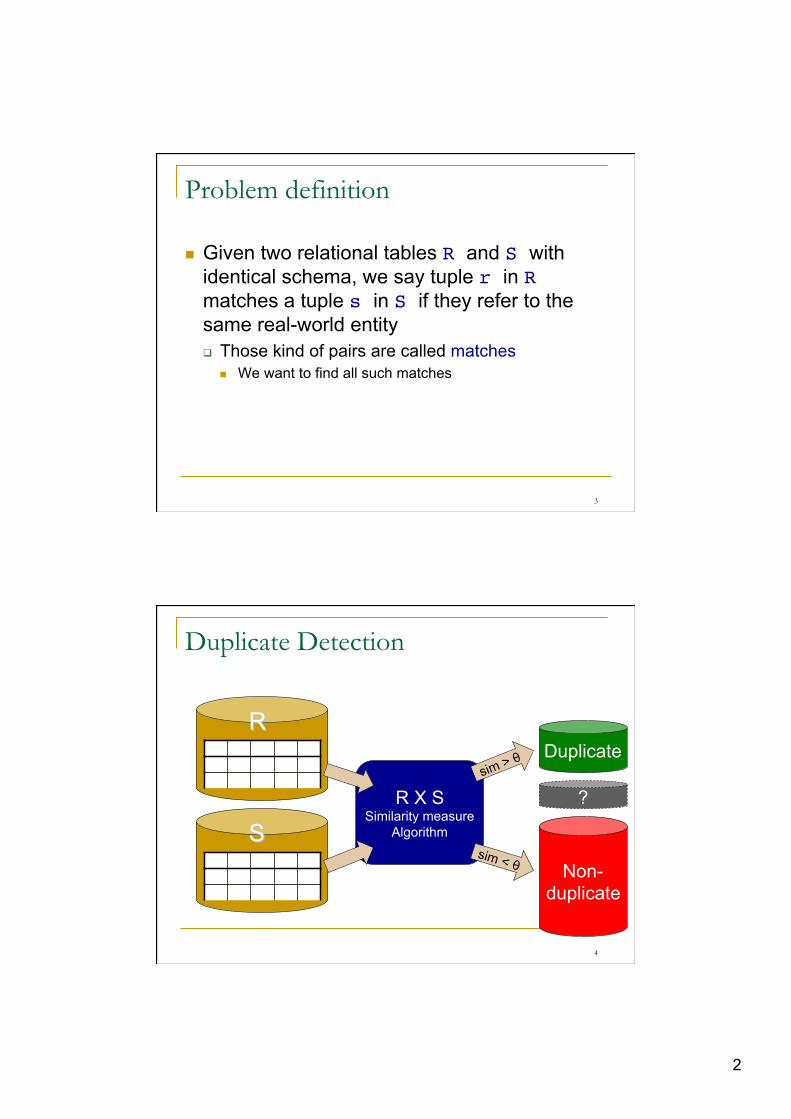
Problem definition

n  Given two relational tables R and S with identical schema, we say tuple r in R matches a tuple s in S if they refer to the same real-world entity q  Those kind of pairs are called matches

n  We want to find all such matches

3

Duplicate Detection

R X S Similarity measure

Algorithm

R

S

sim > θ

sim < θ

Duplicate

Non- duplicate

?

4

3

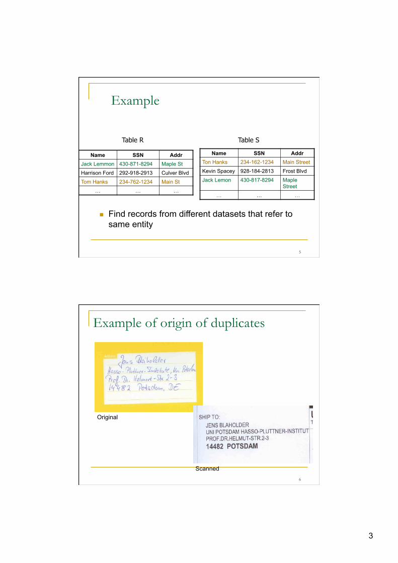
Example

Name SSN Addr Jack Lemmon 430-871-8294 Maple St

Harrison Ford 292-918-2913 Culver Blvd

Tom Hanks 234-762-1234 Main St

… … …

Table R

Name SSN Addr Ton Hanks 234-162-1234 Main Street

Kevin Spacey 928-184-2813 Frost Blvd

Jack Lemon 430-817-8294 Maple Street

… … …

Table S

n  Find records from different datasets that refer to same entity

5

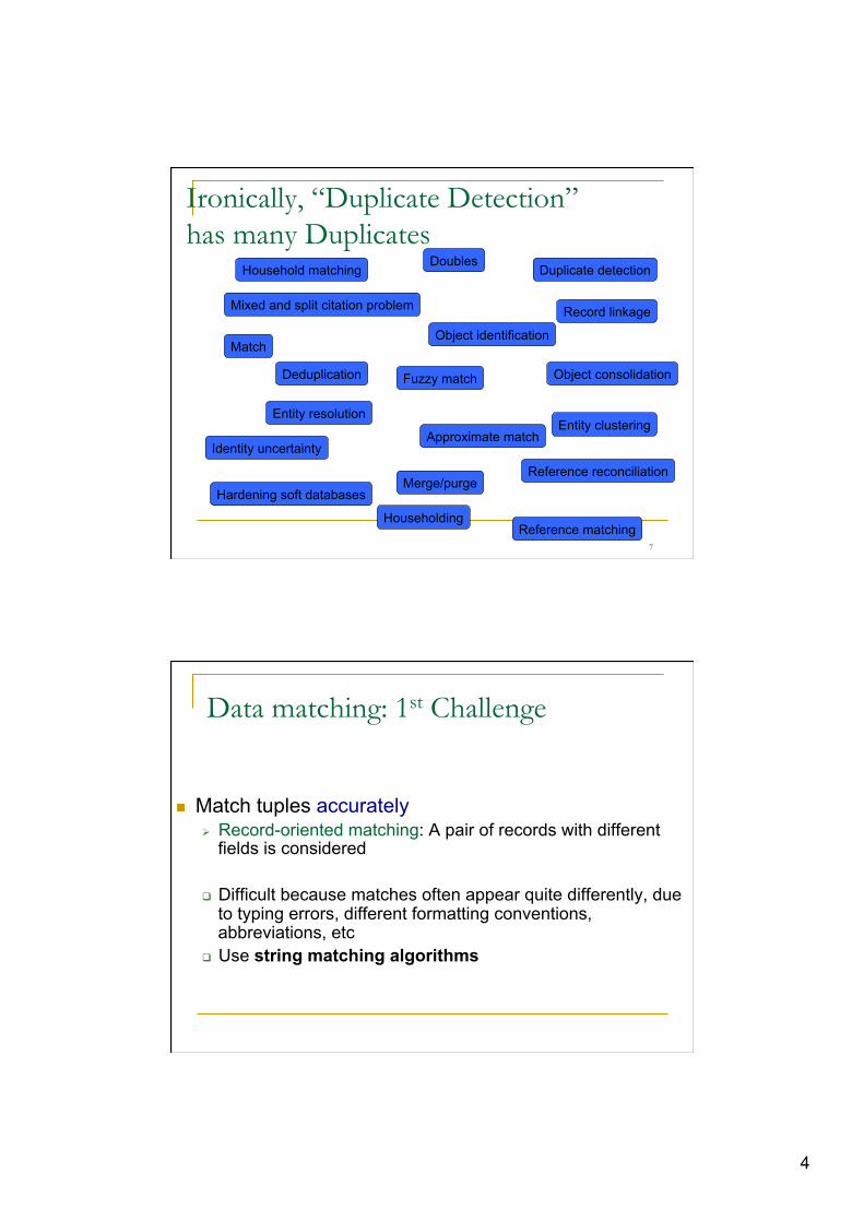
Example of origin of duplicates

Original

Scanned 6

4

Ironically, “Duplicate Detection” has many Duplicates

Doubles Duplicate detection

Record linkage

Deduplication

Object identification

Object consolidation

Entity resolution Entity clustering

Reference reconciliation

Reference matching Householding

Household matching

Match

Fuzzy match

Approximate match

Merge/purge Hardening soft databases

Identity uncertainty

Mixed and split citation problem

7

Data matching: 1st Challenge

n  Match tuples accurately Ø  Record-oriented matching: A pair of records with different

fields is considered

q  Difficult because matches often appear quite differently, due to typing errors, different formatting conventions, abbreviations, etc

q  Use string matching algorithms

5

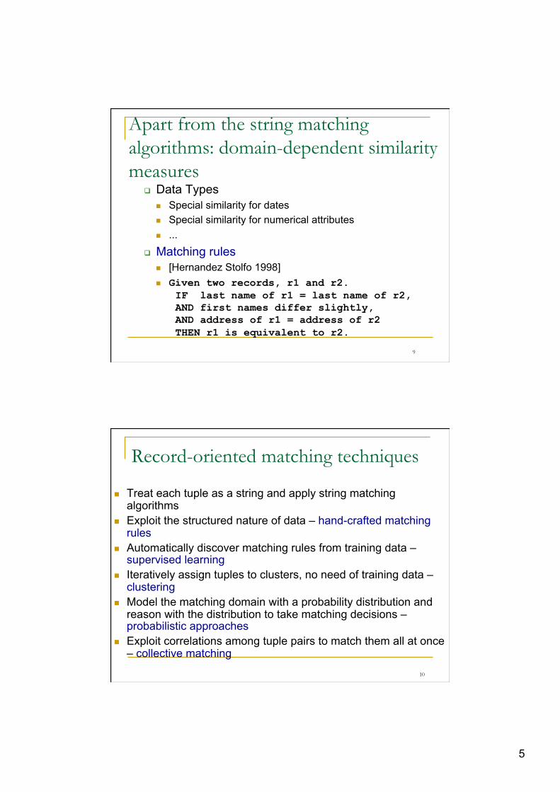
Apart from the string matching algorithms: domain-dependent similarity measures

q  Data Types n  Special similarity for dates n  Special similarity for numerical attributes n  ...

q  Matching rules n  [Hernandez Stolfo 1998] n  Given two records, r1 and r2.

IF last name of r1 = last name of r2, AND first names differ slightly, AND address of r1 = address of r2 THEN r1 is equivalent to r2.

9

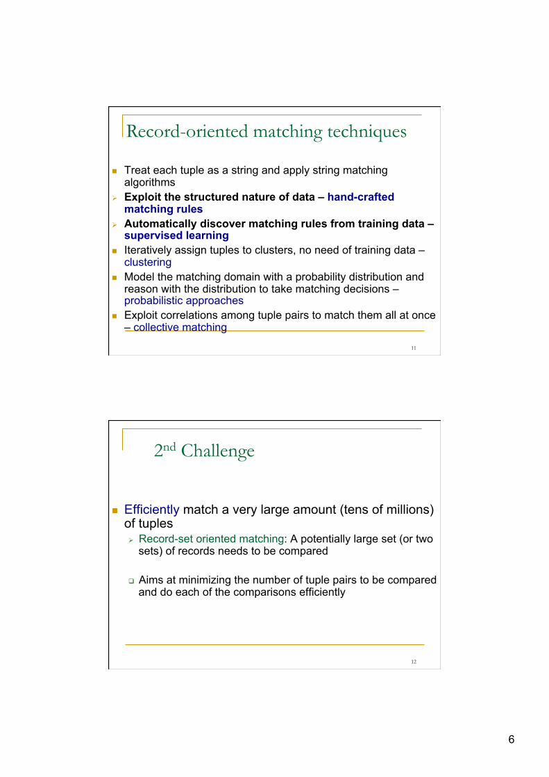
Record-oriented matching techniques

n  Treat each tuple as a string and apply string matching algorithms

n  Exploit the structured nature of data – hand-crafted matching rules

n  Automatically discover matching rules from training data – supervised learning

n  Iteratively assign tuples to clusters, no need of training data – clustering

n  Model the matching domain with a probability distribution and reason with the distribution to take matching decisions – probabilistic approaches

n  Exploit correlations among tuple pairs to match them all at once – collective matching

10

6

n  Treat each tuple as a string and apply string matching algorithms

Ø  Exploit the structured nature of data – hand-crafted matching rules

Ø  Automatically discover matching rules from training data – supervised learning

n  Iteratively assign tuples to clusters, no need of training data – clustering

n  Model the matching domain with a probability distribution and reason with the distribution to take matching decisions – probabilistic approaches

n  Exploit correlations among tuple pairs to match them all at once – collective matching

11

Record-oriented matching techniques

2nd Challenge

n  Efficiently match a very large amount (tens of millions) of tuples Ø  Record-set oriented matching: A potentially large set (or two

sets) of records needs to be compared

q  Aims at minimizing the number of tuple pairs to be compared and do each of the comparisons efficiently

12

7

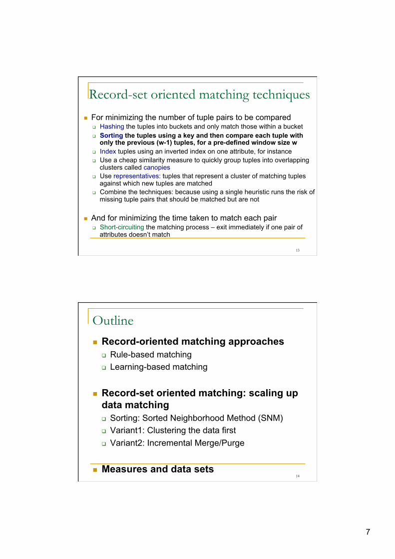
Record-set oriented matching techniques

n  For minimizing the number of tuple pairs to be compared q  Hashing the tuples into buckets and only match those within a bucket q  Sorting the tuples using a key and then compare each tuple with

only the previous (w-1) tuples, for a pre-defined window size w q  Index tuples using an inverted index on one attribute, for instance q  Use a cheap similarity measure to quickly group tuples into overlapping

clusters called canopies q  Use representatives: tuples that represent a cluster of matching tuples

against which new tuples are matched q  Combine the techniques: because using a single heuristic runs the risk of

missing tuple pairs that should be matched but are not

n  And for minimizing the time taken to match each pair q  Short-circuiting the matching process – exit immediately if one pair of

attributes doesn’t match

13

Outline n  Record-oriented matching approaches

q  Rule-based matching q  Learning-based matching

n  Record-set oriented matching: scaling up data matching q  Sorting: Sorted Neighborhood Method (SNM) q  Variant1: Clustering the data first q  Variant2: Incremental Merge/Purge

n  Measures and data sets 14

8

Outline Ø  Record-oriented matching approaches

q  Rule-based matching q  Learning-based matching

n  Record-set oriented matching: scaling up data matching q  Sorting: Sorted Neighborhood Method (SNM) q  Variant1: Clustering the data first q  Variant2: Incremental Merge/Purge

n  Measures and data sets 15

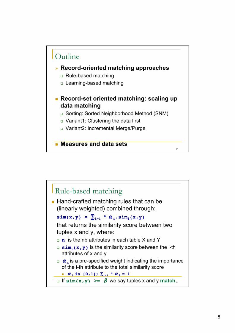
Rule-based matching n  Hand-crafted matching rules that can be

(linearly weighted) combined through: sim(x,y) = ∑i=1 n αi.simi(x,y)!

that returns the similarity score between two tuples x and y, where: q  n is the nb attributes in each table X and Y q  simi(x,y) is the similarity score between the i-th

attributes of x and y q  αi is a pre-specified weight indicating the importance

of the i-th attribute to the total similarity score n  αi in [0,1]; ∑i=1 n αi = 1

q  If sim(x,y) >= β we say tuples x and y match 16

9

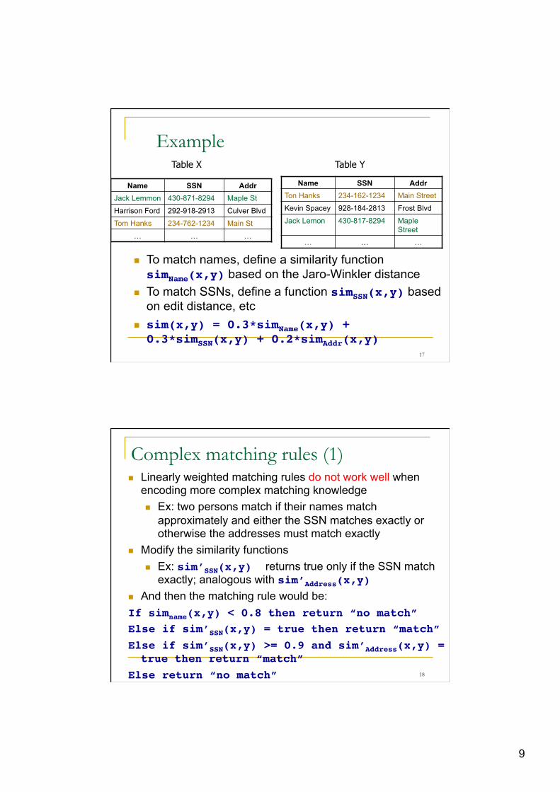
Example

Name SSN Addr Jack Lemmon 430-871-8294 Maple St

Harrison Ford 292-918-2913 Culver Blvd

Tom Hanks 234-762-1234 Main St

… … …

Table X

Name SSN Addr Ton Hanks 234-162-1234 Main Street

Kevin Spacey 928-184-2813 Frost Blvd

Jack Lemon 430-817-8294 Maple Street

… … …

Table Y

n  To match names, define a similarity function simName(x,y) based on the Jaro-Winkler distance

n  To match SSNs, define a function simSSN(x,y) based on edit distance, etc

n  sim(x,y) = 0.3*simName(x,y) + 0.3*simSSN(x,y) + 0.2*simAddr(x,y)!

17

Complex matching rules (1) n  Linearly weighted matching rules do not work well when

encoding more complex matching knowledge n  Ex: two persons match if their names match

approximately and either the SSN matches exactly or otherwise the addresses must match exactly

n  Modify the similarity functions n  Ex: sim’SSN(x,y) returns true only if the SSN match

exactly; analogous with sim’Address(x,y) !n  And then the matching rule would be: If simname(x,y) < 0.8 then return “no match”!Else if sim’SSN(x,y) = true then return “match”!Else if sim’SSN(x,y) >= 0.9 and sim’Address(x,y) = true then return “match”!

Else return “no match”! 18

10

Complex matching rules (2)

n  This kind of rules are often written in a high-level declarative language n  Easier to understand, debug, modify and maintain

n  Still, it is labor intensive to write good matching rules n  Or not clear at all how to write them n  Or difficult to set the parameters α,β

19

Learning-based matching

q  Supervised learning n  can also be unsupervised (clustering)

q  Idea: learn a matching model M from the training data, then apply M to match new tuple pairs.

q  Training data has the form: T = {(x1, y1, l1), (x2, y2, l2), …,(xn, yn, ln)}!

where each triple (xi, yi, li) consists of a tuple pair (xi, yi) and a label li with value “yes” if xi matches yi and “no” otherwise.

20

11

Training (1)

n  Define a set of features f1, f2, …, fm thought to be potentially relevant to matching q  each fi quantifies one aspect of the domain

judged possibly relevant to matching the tuples q  Each feature fi is a function that takes a tuple

pair (x,y) and produces a numerical, categorical, or binary value.

n  The learning algorithm will use the training data to decide which features are in fact relevant

21

Training (2)

n  Convert each training example (xi, yi, li) in the set T into a pair:

(<f1(xi, yi), f2(xi, yi),… fm(xi, yi)>, ci)! where Vi = <f1(xi, yi), f2(xi, yi),… fm(xi, yi)>! is a feature vector that encodes the tuple pair (xi,yi)! in terms of the features and ci is an appropriately transformed version of label li!

n  Training set T is converted into a new training set T’: {(v1, c1), (v2, c2), …, (vn, cn)} ! and then we apply a learning algorithm such as SVM or Decision Trees to T’ to learn a matching model M

22

12

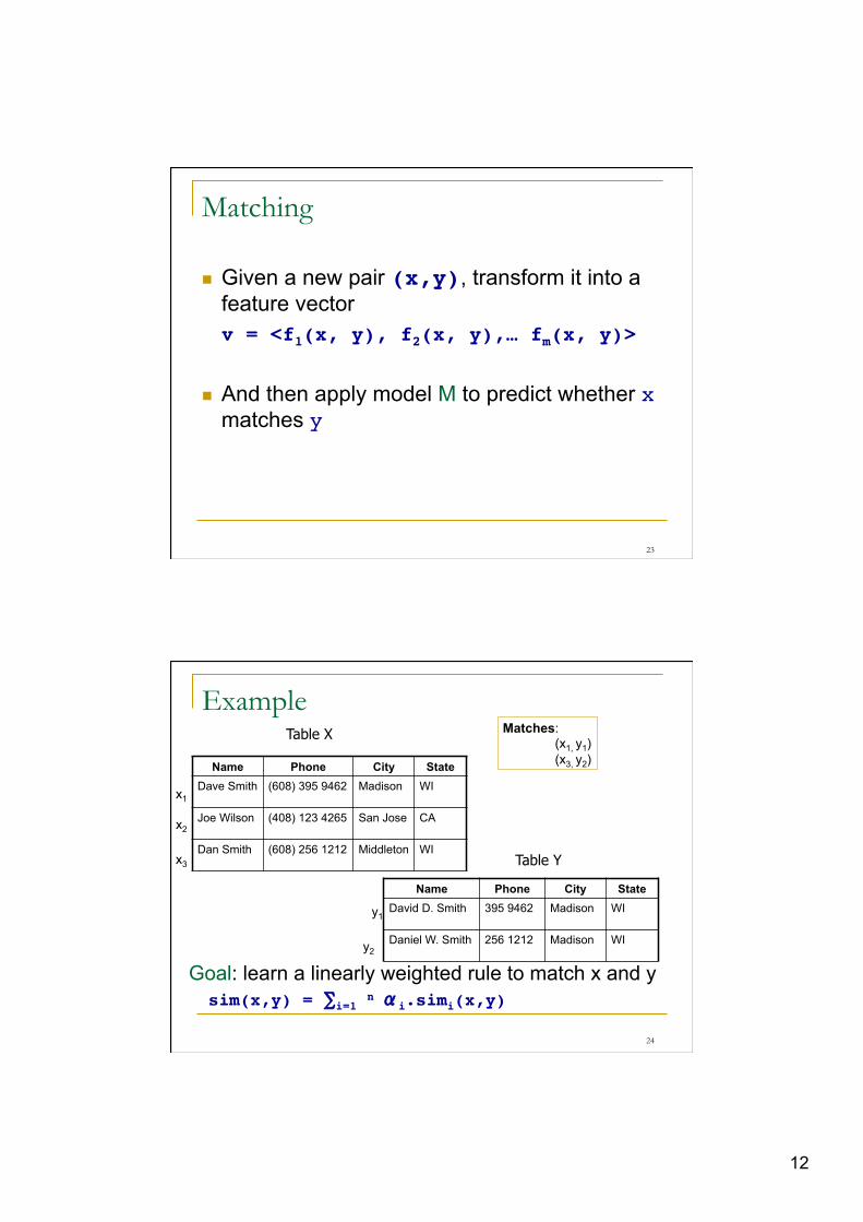
Matching

n  Given a new pair (x,y), transform it into a feature vector !v = <f1(x, y), f2(x, y),… fm(x, y)>!!

n  And then apply model M to predict whether x matches y !

23

Example

Name Phone City State Dave Smith (608) 395 9462 Madison WI

Joe Wilson (408) 123 4265 San Jose CA

Dan Smith (608) 256 1212 Middleton WI

Table X

Table Y

Name Phone City State David D. Smith 395 9462 Madison WI

Daniel W. Smith 256 1212 Madison WI

x2

x1

y1

y2

x3

Goal: learn a linearly weighted rule to match x and y sim(x,y) = ∑i=1 n αi.simi(x,y)!

Matches: (x1, y1) (x3, y2)

24

13

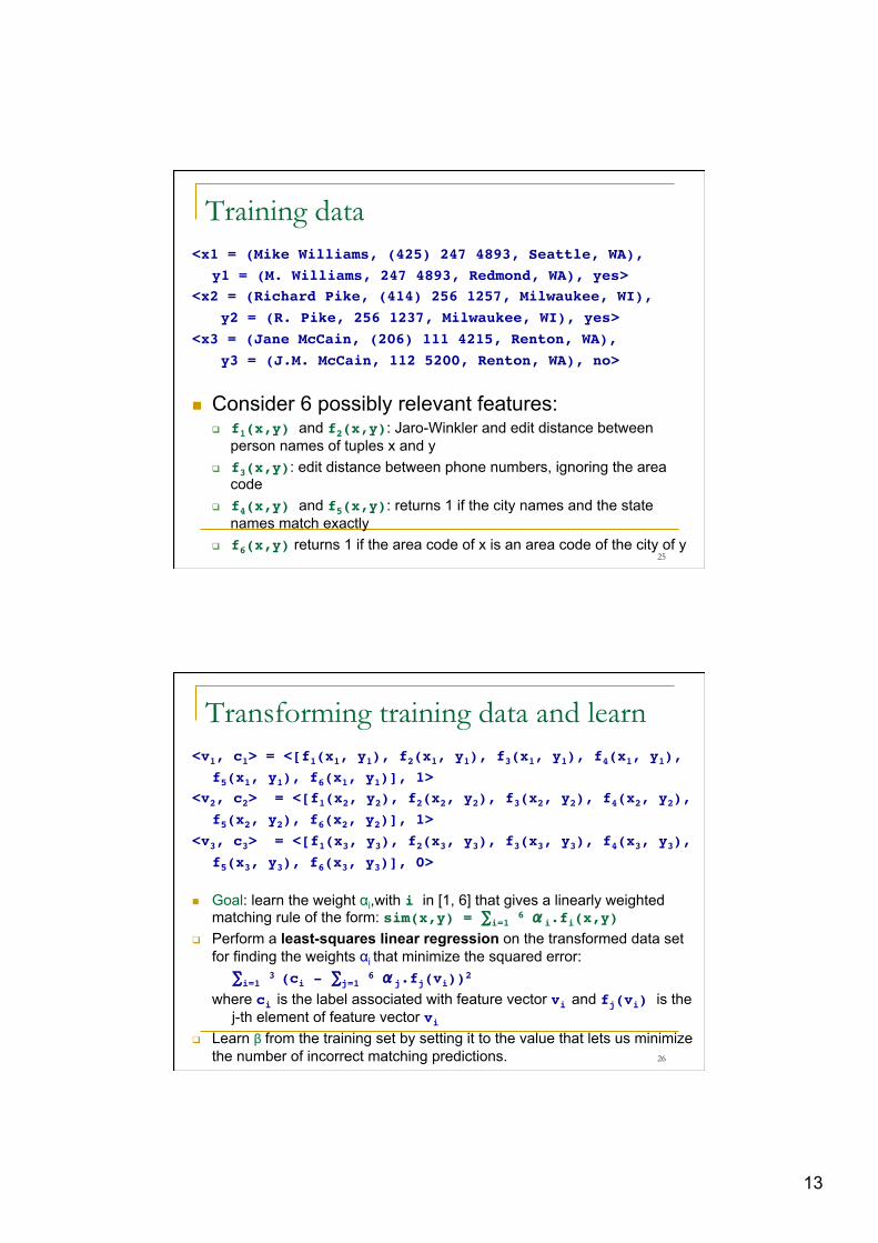
Training data <x1 = (Mike Williams, (425) 247 4893, Seattle, WA), ! !y1 = (M. Williams, 247 4893, Redmond, WA), yes>!<x2 = (Richard Pike, (414) 256 1257, Milwaukee, WI), !! y2 = (R. Pike, 256 1237, Milwaukee, WI), yes>!

<x3 = (Jane McCain, (206) 111 4215, Renton, WA),!! y3 = (J.M. McCain, 112 5200, Renton, WA), no>!

!

n  Consider 6 possibly relevant features: q  f1(x,y) and f2(x,y): Jaro-Winkler and edit distance between

person names of tuples x and y q  f3(x,y): edit distance between phone numbers, ignoring the area

code q  f4(x,y) and f5(x,y): returns 1 if the city names and the state

names match exactly q  f6(x,y) returns 1 if the area code of x is an area code of the city of y

25

Transforming training data and learn <v1, c1> = <[f1(x1, y1), f2(x1, y1), f3(x1, y1), f4(x1, y1), !!f5(x1, y1), f6(x1, y1)], 1>!

<v2, c2> = <[f1(x2, y2), f2(x2, y2), f3(x2, y2), f4(x2, y2), !!f5(x2, y2), f6(x2, y2)], 1>!

<v3, c3> = <[f1(x3, y3), f2(x3, y3), f3(x3, y3), f4(x3, y3), !!f5(x3, y3), f6(x3, y3)], 0>!

n  Goal: learn the weight αi,with i in [1, 6] that gives a linearly weighted matching rule of the form: sim(x,y) = ∑i=1 6 αi.fi(x,y)!

q  Perform a least-squares linear regression on the transformed data set for finding the weights αi that minimize the squared error: !∑i=1 3 (ci - ∑j=1 6 αj.fj(vi))2!

where ci is the label associated with feature vector vi and fj(vi) is the j-th element of feature vector vi!

q  Learn β from the training set by setting it to the value that lets us minimize the number of incorrect matching predictions.

!

!

!

26

14

Advantages/inconvenients supervised learning

n  Advantages: q  Can automatically examine a large set of features

to select the most useful ones q  Can construct very complex rules, very difficult to

construct in rule-based learning n  Inconvenients:

q  Requires a large number of training examples which can be labor intensive to obtain

27

Outline

n  Matching approaches q  Rule-based matching q  Learning-based matching

Ø  Scaling up data matching q  Sorting: Sorted Neighborhood Method (SNM) q  Incremental Merge/Purge

n  Measures and data sets q  Recall, precision, F-measure

28

15

Record Pairs as Matrix

1 2 3 4 5 6 7 8 9 10

11

12

13

14

15

16

17

18

19

20

1

2

3

4

5

6

7

8

9

10

11

12

13

14

15

16

17

18

19

20

29

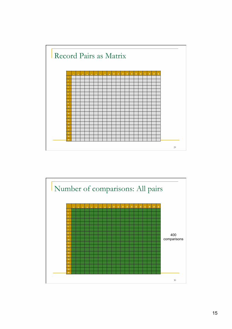
Number of comparisons: All pairs

1 2 3 4 5 6 7 8 9 10

11

12

13

14

15

16

17

18

19

20

1

2

3

4

5

6

7

8

9

10

11

12

13

14

15

16

17

18

19

20

400 comparisons

30

16

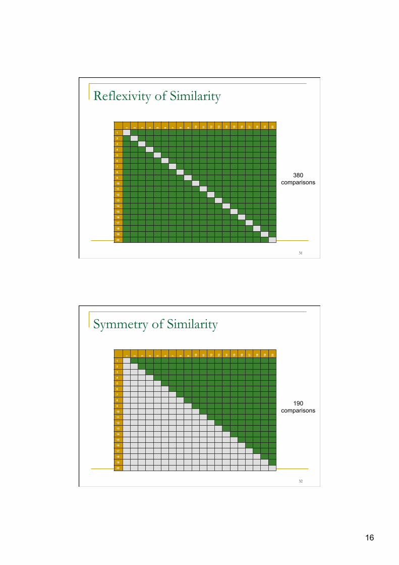
Reflexivity of Similarity

1 2 3 4 5 6 7 8 9 10

11

12

13

14

15

16

17

18

19

20

1

2

3

4

5

6

7

8

9

10

11

12

13

14

15

16

17

18

19

20

380 comparisons

31

Symmetry of Similarity

1 2 3 4 5 6 7 8 9 10

11

12

13

14

15

16

17

18

19

20

1

2

3

4

5

6

7

8

9

10

11

12

13

14

15

16

17

18

19

20

190 comparisons

32

17

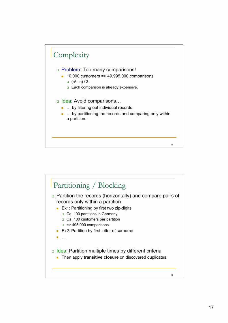
Complexity

q  Problem: Too many comparisons! n  10.000 customers => 49.995.000 comparisons

q  (n² - n) / 2 q  Each comparison is already expensive.

q  Idea: Avoid comparisons… n  … by filtering out individual records. n  … by partitioning the records and comparing only within

a partition.

33

Partitioning / Blocking q  Partition the records (horizontally) and compare pairs of

records only within a partition n  Ex1: Partitioning by first two zip-digits

q  Ca. 100 partitions in Germany q  Ca. 100 customers per partition q  => 495.000 comparisons

n  Ex2: Partition by first letter of surname n  …

q  Idea: Partition multiple times by different criteria n  Then apply transitive closure on discovered duplicates.

34

18

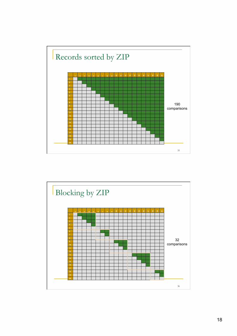
Records sorted by ZIP

1 2 3 4 5 6 7 8 9 10

11

12

13

14

15

16

17

18

19

20

1

2

3

4

5

6

7

8

9

10

11

12

13

14

15

16

17

18

19

20

190 comparisons

35

Blocking by ZIP

1 2 3 4 5 6 7 8 9 10

11

12

13

14

15

16

17

18

19

20

1

2

3

4

5

6

7

8

9

10

11

12

13

14

15

16

17

18

19

20

32 comparisons

36

19

Record-set oriented matching techniques (recap.)

n  For minimizing the number of tuple pairs to be compared q  Hashing the tuples into buckets and only match those within a bucket q  Sorting the tuples using a key and then compare each tuple with only the

previous (w-1) tuples, for a pre-defined window size w q  Index tuples using an inverted index on one attribute, for instance q  Use a cheap similarity measure to quickly group tuples into overlapping

clusters called canopies q  Use representatives: tuples that represent a cluster of matching tuples

against which new tuples are matched q  Combine the techniques: because suing a single heuristic runs the risk of

missing tuple pairs that should be matched but are not

n  And for minimizing the time taken to match each pair q  Short-circuiting the matching process – exit immediately if one pair of

attributes doesn’t match

37

Sorted Neighbourhood Method - SNM (or Windowing)

n  Concatenate all records to be matched in a single file (or table)

n  Sort the records using a pre-defined key based on the values of the attributes for each record

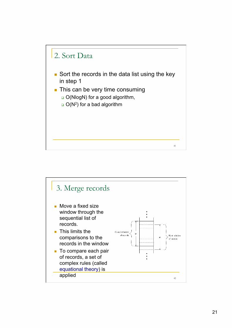
n  Move a window of a specific size w over the file, comparing only the records that belong to this window

38

20

Sorted Neighborhood Method in detail

1.  Create Key: Compute a key K for each record in the list by extracting relevant fields or portions of fields. q  Relevance is decided by experts.

2.  Sort Data: Sort the records in the data list using K !3.  Merge: Move a fixed size window through the

sequential list of records limiting the comparisons for matching records to those records in the window. If the size of the window is w records, then every new record entering the window is compared with the previous records to find “matching” records

39

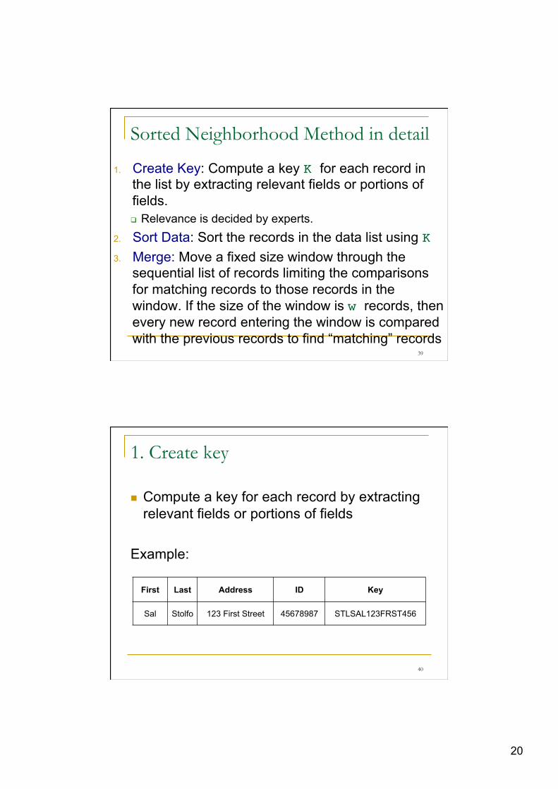
1. Create key

n  Compute a key for each record by extracting relevant fields or portions of fields

Example:

First Last Address ID Key

Sal Stolfo 123 First Street 45678987 STLSAL123FRST456

40

21

2. Sort Data

n  Sort the records in the data list using the key in step 1

n  This can be very time consuming q  O(NlogN) for a good algorithm, q  O(N2) for a bad algorithm

41

3. Merge records

n  Move a fixed size window through the sequential list of records.

n  This limits the comparisons to the records in the window

n  To compare each pair of records, a set of complex rules (called equational theory) is applied

42

22

Considerations

n  What is the optimal window size while q  Maximizing accuracy q  Minimizing computational cost

n  The effectiveness of the SNM highly depends on the key selected to sort the records q  A key is defined to be a sequence of a subset of

attributes q  Keys must provide sufficient discriminating power

43

Example of Records and Keys

First Last Address ID Key

Sal Stolfo 123 First Street 45678987 STLSAL123FRST456

Sal Stolfo 123 First Street 45678987 STLSAL123FRST456

Sal Stolpho 123 First Street 45678987 STLSAL123FRST456

Sal Stiles 123 Forest Street 45654321 STLSAL123FRST456

44

23

Equational Theory (record matching rules)

n  The comparison during the merge phase is an inferential process

n  Compares much more information than simply the key

n  The more information there is, the better inferences can be made

45

Equational Theory - Example

n  Two names are spelled nearly identically and have the same address q  It may be inferred that they are the same person

n  Two social security numbers are the same but the names and addresses are totally different q  Could be the same person who moved q  Could be two different people and there is an

error in the social security number

46

24

A simplified rule in English

Given two records, r1 and r2!IF the last name of r1 equals the last name of r2,!

AND the first names differ slightly,!AND the address of r1 equals the address of r2!

THEN!!r1 is equivalent to r2!

!

47

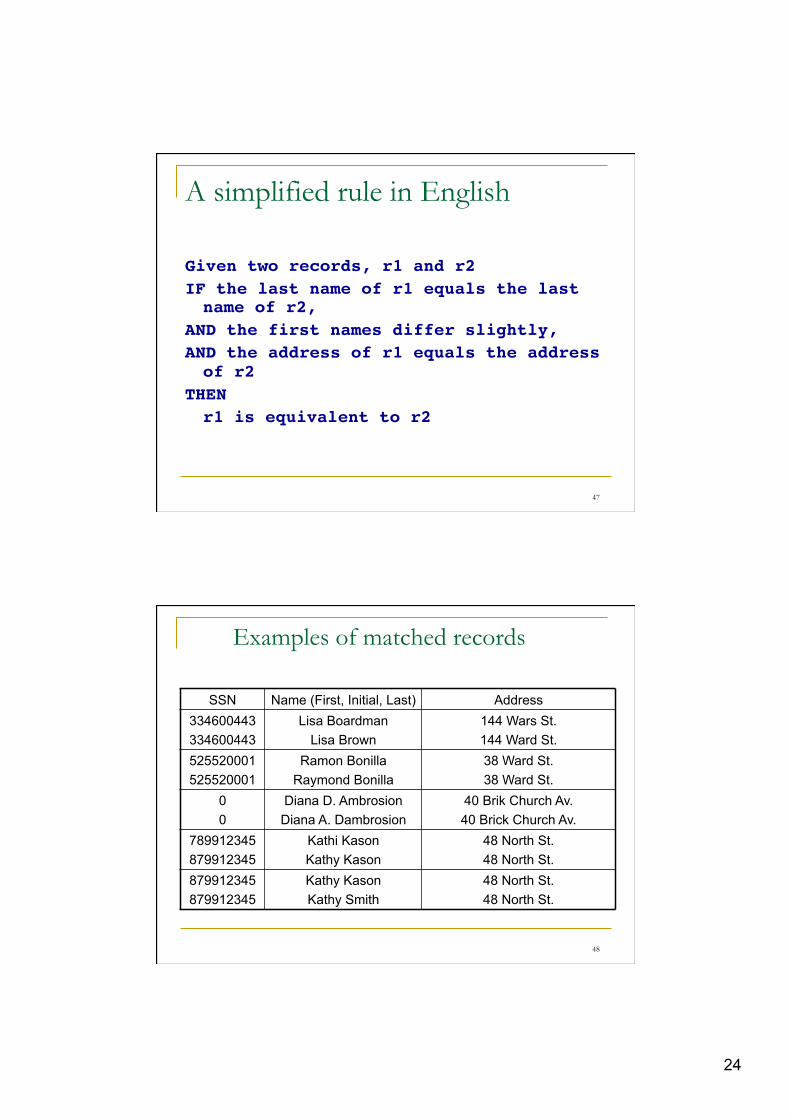
Examples of matched records

SSN Name (First, Initial, Last) Address 334600443 334600443

Lisa Boardman Lisa Brown

144 Wars St. 144 Ward St.

525520001 525520001

Ramon Bonilla Raymond Bonilla

38 Ward St. 38 Ward St.

0 0

Diana D. Ambrosion Diana A. Dambrosion

40 Brik Church Av. 40 Brick Church Av.

789912345 879912345

Kathi Kason Kathy Kason

48 North St. 48 North St.

879912345 879912345

Kathy Kason Kathy Smith

48 North St. 48 North St.

48

25

Building an equational theory

n  The process of creating a good equational theory is similar to the process of creating a good knowledge-base for an expert system

n  In complex problems, an expert’s assistance is needed to write the equational theory

49

Looses some matching pairs

n  In general, no single pass (i.e. no single key) will be sufficient to catch all matching records

n  An attribute that appears first in the key has higher discriminating power than those appearing after them q  If an employee has two records in a DB with SSN

193456782 and 913456782, it’s unlikely they will fall under the same window

50

26

Possible solutions

n  Goal: To increase the number of similar records being matched

n  Widen the scanning window size, w n  Execute several independent runs of the SNM

q Use a different key each time q Use a relatively small window q Call this the Multi-Pass approach

51

Multi-pass approach

n  Each independent run of the Multi-Pass approach will produce a set of pairs of records q  Although one field in a record may be in error,

another field may not

n  Transitive closure can be applied to those pairs to be merged

52

27

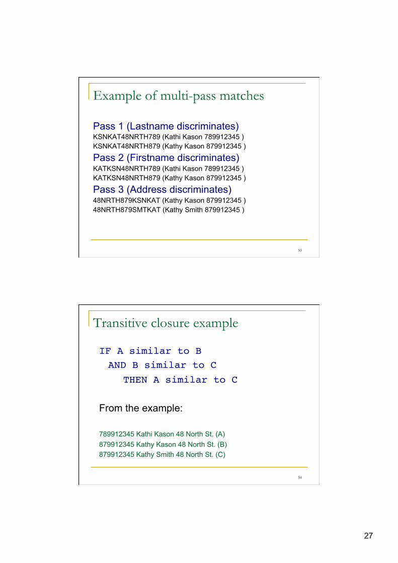
Example of multi-pass matches

Pass 1 (Lastname discriminates) KSNKAT48NRTH789 (Kathi Kason 789912345 ) KSNKAT48NRTH879 (Kathy Kason 879912345 )

Pass 2 (Firstname discriminates) KATKSN48NRTH789 (Kathi Kason 789912345 ) KATKSN48NRTH879 (Kathy Kason 879912345 )

Pass 3 (Address discriminates) 48NRTH879KSNKAT (Kathy Kason 879912345 ) 48NRTH879SMTKAT (Kathy Smith 879912345 )

53

Transitive closure example

IF A similar to B!!AND B similar to C!! !THEN A similar to C!!From the example: 789912345 Kathi Kason 48 North St. (A) 879912345 Kathy Kason 48 North St. (B) 879912345 Kathy Smith 48 North St. (C)

54

28

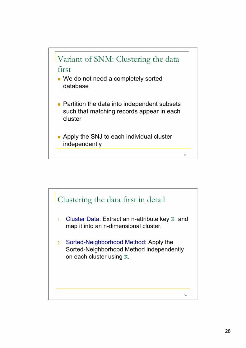
Variant of SNM: Clustering the data first n  We do not need a completely sorted

database n  Partition the data into independent subsets

such that matching records appear in each cluster

n  Apply the SNJ to each individual cluster independently

55

Clustering the data first in detail

1.  Cluster Data: Extract an n-attribute key K and map it into an n-dimensional cluster.

2.  Sorted-Neighborhood Method: Apply the Sorted-Neighborhood Method independently on each cluster using K.

56

29

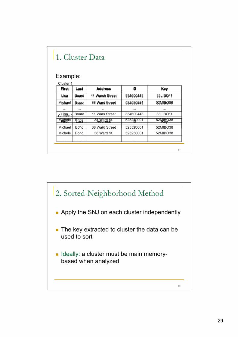
1. Cluster Data

Example:

First Last Address ID Key

Lisa Board 11 Warsh Street 334600443 33LIBO11

Michael Bond 38 Ward Street 525520001 52MIBO38 … … … … …

Lisa Board 11 Wars Street 334600443 33LIBO11 Michele Bond 38 Ward St. 525250001 52MIBO38 … … … … …

Cluster 2 First Last Address ID Key

Michael Bond 38 Ward Street 525520001 52MIBO38 Michele Bond 38 Ward St. 525250001 52MIBO38 … … … … …

Cluster 1 First Last Address ID Key

Lisa Board 11 Warsh Street 334600443 33LIBO11

Lisa Board 11 Wars Street 334600443 33LIBO11 … … … … …

57

2. Sorted-Neighborhood Method

n  Apply the SNJ on each cluster independently

n  The key extracted to cluster the data can be used to sort

n  Ideally: a cluster must be main memory-based when analyzed

58

30

Another SNM variant: Incremental Merge/Purge

n  Lists of records are concatenated for first time processing

n  Concatenating new data records before reapplying the merge/purge process may be very expensive in both time and space

n  An incremental merge/purge approach is needed: Prime Representatives method

59

Prime-Representative (PR)

n  Prime-Representative: set of records extracted from each cluster of records to represent the information in that cluster

n  Initially, no Prime-Representative exists n  After the execution of the first merge/purge,

clusters of similar records are created n  Correct selection of PR from cluster impacts

accuracy of results

60

31

Some strategies for choosing PR

n  Random Sample q  Select a sample of records at random from each

cluster n  N-Latest

q  Most recent elements entered in DB n  Syntactic

q  Choose the largest or more complete record

61

Outline

n  Matching approaches q  Rule-based matching q  Learning-based matching

n  Scaling up data matching q  Sorting: Sorted Neighborhood Method (SNM) q  Incremental Merge/Purge

Ø  Measures and data sets q  Recall, precision, F-measure

62

32

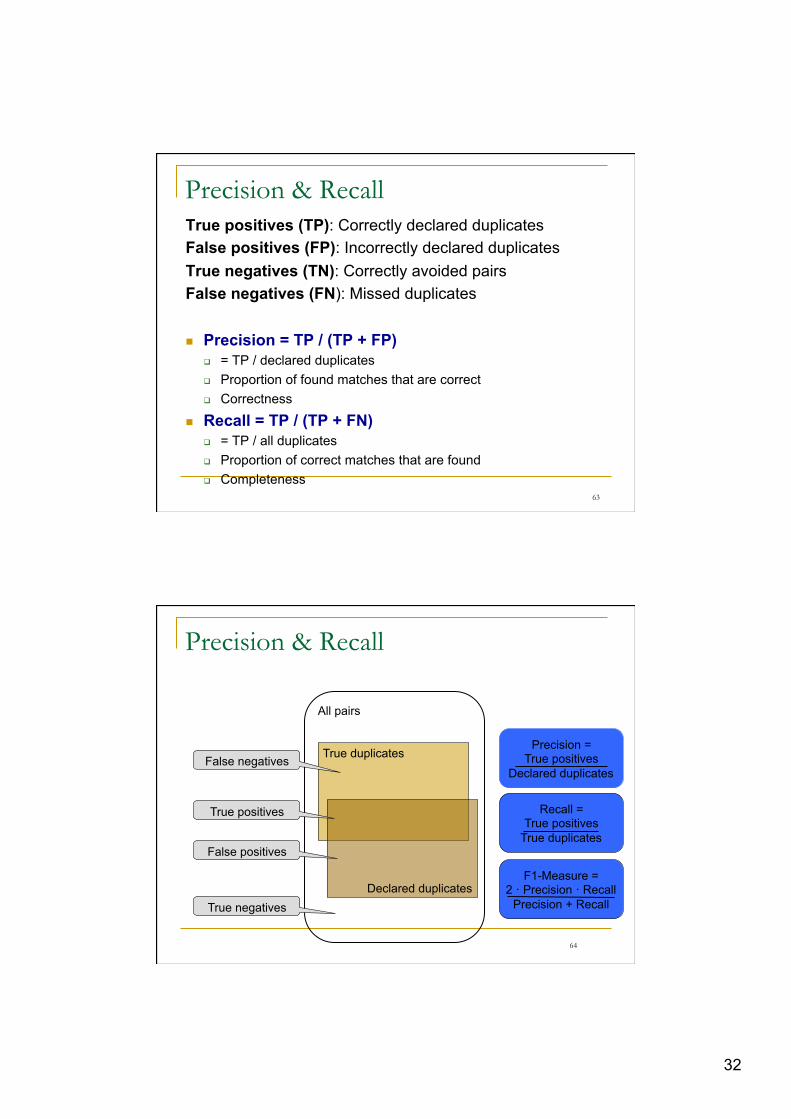
Precision & Recall True positives (TP): Correctly declared duplicates False positives (FP): Incorrectly declared duplicates True negatives (TN): Correctly avoided pairs False negatives (FN): Missed duplicates

n  Precision = TP / (TP + FP) q  = TP / declared duplicates q  Proportion of found matches that are correct q  Correctness

n  Recall = TP / (TP + FN) q  = TP / all duplicates q  Proportion of correct matches that are found q  Completeness

63

Precision & Recall

64

All pairs

True duplicates

Declared duplicates

False negatives

True negatives

False positives

True positives

Precision = True positives

Declared duplicates

Recall = True positives

True duplicates

F1-Measure = 2 · Precision · Recall

Precision + Recall

33

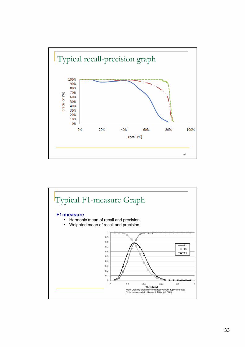
Typical recall-precision graph

65

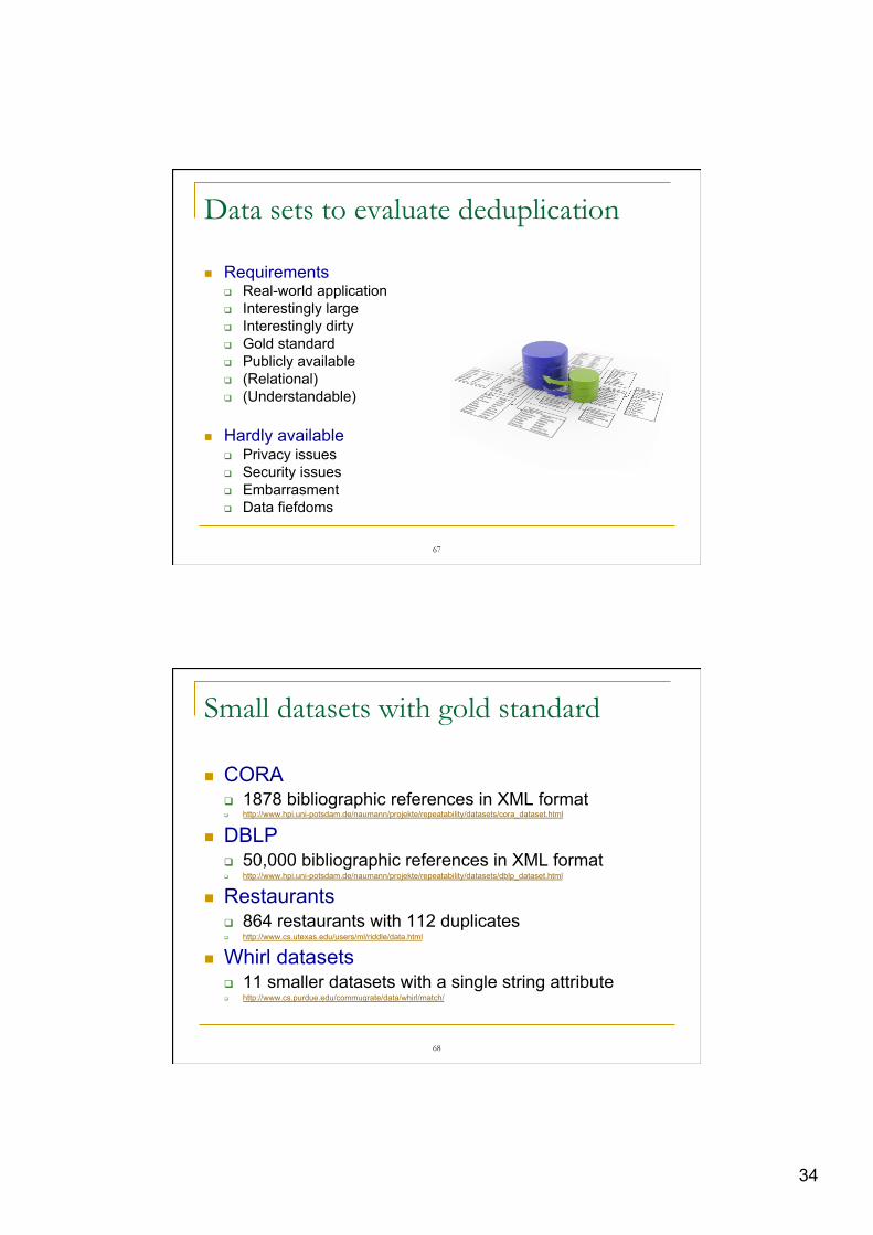
From Creating probabilistic databases from duplicated data Oktie Hassanzadeh · Renée J. Miller (VLDBJ)

Typical F1-measure Graph

F1-measure •  Harmonic mean of recall and precision •  Weighted mean of recall and precision

34

Data sets to evaluate deduplication

n  Requirements q  Real-world application q  Interestingly large q  Interestingly dirty q  Gold standard q  Publicly available q  (Relational) q  (Understandable)

n  Hardly available q  Privacy issues q  Security issues q  Embarrasment q  Data fiefdoms

67

Small datasets with gold standard

n  CORA q  1878 bibliographic references in XML format q  http://www.hpi.uni-potsdam.de/naumann/projekte/repeatability/datasets/cora_dataset.html

n  DBLP q  50,000 bibliographic references in XML format q  http://www.hpi.uni-potsdam.de/naumann/projekte/repeatability/datasets/dblp_dataset.html

n  Restaurants q  864 restaurants with 112 duplicates q  http://www.cs.utexas.edu/users/ml/riddle/data.html

n  Whirl datasets q  11 smaller datasets with a single string attribute q  http://www.cs.purdue.edu/commugrate/data/whirl/match/

68

35

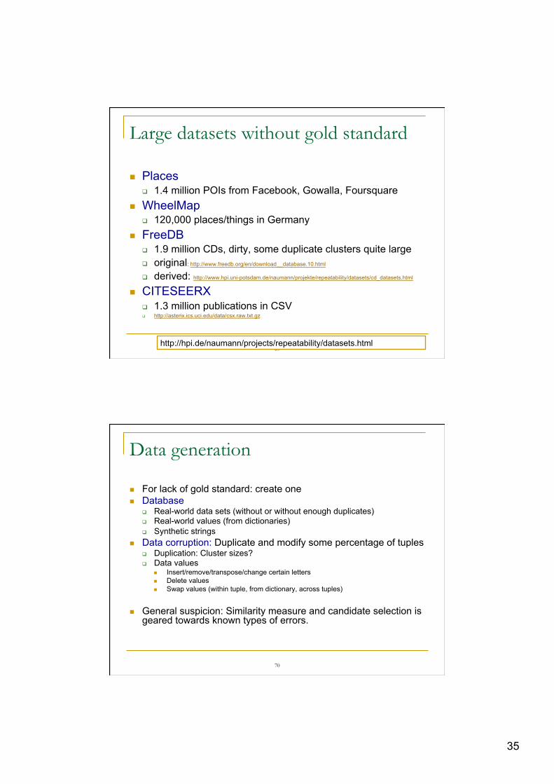
Large datasets without gold standard

n  Places q  1.4 million POIs from Facebook, Gowalla, Foursquare

n  WheelMap q  120,000 places/things in Germany

n  FreeDB q  1.9 million CDs, dirty, some duplicate clusters quite large q  original: http://www.freedb.org/en/download__database.10.html

q  derived: http://www.hpi.uni-potsdam.de/naumann/projekte/repeatability/datasets/cd_datasets.html

n  CITESEERX q  1.3 million publications in CSV q  http://asterix.ics.uci.edu/data/csx.raw.txt.gz

69 http://hpi.de/naumann/projects/repeatability/datasets.html

Data generation

n  For lack of gold standard: create one n  Database

q  Real-world data sets (without or without enough duplicates) q  Real-world values (from dictionaries) q  Synthetic strings

n  Data corruption: Duplicate and modify some percentage of tuples q  Duplication: Cluster sizes? q  Data values

n  Insert/remove/transpose/change certain letters n  Delete values n  Swap values (within tuple, from dictionary, across tuples)

n  General suspicion: Similarity measure and candidate selection is geared towards known types of errors.

70

36

Data generators

n  UIS Database Generator q  Generates a list of randomly perturbed names and US mailing

addresses. q  Written by Mauricio Hernández. q  http://www.cs.utexas.edu/users/ml/riddle/data/dbgen.tar.gz

n  FEBRL-Generator q  Part of a cleansing suite q  Dictionaries with frequencies q  http://sourceforge.net/projects/febrl/

n  Dirty XML Generator q  http://www.hpi.uni-potsdam.de/naumann/projekte/

completed_projects/dirtyxml.html

71

Next Lecture

n  Data Fusion