Embed Size (px)
Citation preview
1
Deep learning tackles single-cell analysis – A survey of deep learning for scRNA-seq analysis Mario Flores1§, Zhentao Liu1, Tinghe Zhang1, Md Musaddaqui Hasib1, Yu-Chiao Chiu2, Zhenqing Ye2,3, Karla Paniagua1, Sumin Jo1, Jianqiu Zhang1, Shou-Jiang Gao4,6, Yu-Fang Jin1, Yidong Chen2,3§, and Yufei Huang5,6§
1Department of Electrical and Computer Engineering, the University of Texas at San Antonio, San
Antonio, TX 78249, USA
2Greehey Children’s Cancer Research Institute, University of Texas Health San Antonio, San
Antonio, TX 78229, USA
3Department of Population Health Sciences, University of Texas Health San Antonio, San
Antonio, TX 78229, USA
4Department of Microbiology and Molecular Genetics, University of Pittsburgh, Pittsburgh,
Pennsylvania, PA 15232, USA
5Department of Medicine, School of Medicine, University of Pittsburgh, PA 15232, USA
6UPMC Hillman Cancer Center, University of Pittsburgh, PA 15232, USA
§Correspondence should be addressed to Mario Flores ([email protected]);
Yidong Chen ([email protected]); Yufei Huan ([email protected])
Running title: Deep learning for single-cell RNA-seq analysis
Mario Flores, Ph.D., is an Assistant Professor in the Department of Electrical and Computer
Engineering at the University of Texas at San Antonio, His research focuses on DNA and RNA
2
sequence methods, transcriptomics analysis (including scRNA-Seq), epigenetics, comparative
genomics, and deep learning to study mechanisms of gene regulation.
Zhentao Liu is a Ph.D. student in the Department of Electrical and Computer Engineering, the
University of Texas at San Antonio. His research focuses on deep learning for cancer genomics
and drug response prediction.
Tinghe Zhang is a Ph.D. student in the Department of Electrical and Computer Engineering, the
University of Texas at San Antonio. His research focuses on deep learning for cancer genomics
and drug response prediction.
Md Musaddaqui Hasib is a Ph.D. student in the Department of Electrical and Computer
Engineering, the University of Texas at San Antonio. His research focuses on interpretable deep
learning for cancer genomics.
Zhenqing Ye Ph.D., is an Assistant Professor in the Department of Population Health Sciences
and the director of Computational Biology and Bioinformatics at Greehey Children’s Cancer
Research Institute at the University of Texas Health San Antonio. His research focuses on
computational methods on next-generation sequencing and single-cell RNA-seq data analysis.
Sumin Jo is a Ph.D. student in the Department of Electrical and Computer Engineering, the
University of Texas at San Antonio. Her research focuses on m6A mRNA methylation and deep
learning for biomedical applications.
Karla Paniagua is a Ph.D. student in the Department of Electrical and Computer Engineering,
the University of Texas at San Antonio. Her research focuses on applications of deep learning
algorithms.
Yu-Chiao Chiu. Ph.D., is a Postdoctoral Fellow at the Greehey Children’s Cancer Research
Institute at the University of Texas Health San Antonio. His postdoctoral research is focused on
developing deep learning models for pharmacogenomic studies.

3
Jianqiu Zhang, PhD, is an Associate Professor in the Department of Electrical and Computer
Engineering at the University of Texas at San Antonio. Her current research focuses on deep
learning for biomedical applications such as m6A mRNA methylation.
Shou-Jiang Gao, Ph.D., is a Professor in UPMC Hillman Cancer Center and Department of
Microbiology and Molecular Genetics, University of Pittsburgh. His current research interests
include Kaposi’s sarcoma-associate herpesvirus (KSHV), AIDS-related malignancies,
translational and cancer therapeutics, and systems biology.
Yu-Fang Jin, Ph.D., is a Professor in the Department of Electrical and Computer Engineering at
the University of Texas at San Antonio. Her research focuses on mathematical modeling of
cellular responses in immune systems, data-driven modeling and analysis of macrophage
activations, and deep learning applications.
Yidong Chen, Ph.D., is a Professor in the Department of Population Health Sciences and the
director of Computational Biology and Bioinformatics at Greehey Children’s Cancer Research
Institute at the University of Texas Health San Antonio. His research interests include
bioinformatics methods in next-generation sequencing technologies, integrative genomic data
analysis, genetic data visualization and management, and machine learning in translational
cancer research
Yufei Huang, Ph.D., is a Professor in UPMC Hillman Cancer Center and Department of
Medicine, University of Pittsburgh School of Medicine. His current research interests include
uncovering the functions of m6A mRNA methylation, cancer virology, and medical AI & deep
learning.

4
Abstract Since its selection as the method of the year in 2013, single-cell technologies have
become mature enough to provide answers to complex research questions. With the
growth of single-cell profiling technologies, there has also been a significant increase in
data collected from single-cell profilings, resulting in computational challenges to process
these massive and complicated datasets. To address these challenges, deep learning
(DL) is positioning as a competitive alternative for single-cell analyses besides the
traditional machine learning approaches. Here we present a processing pipeline of single-
cell RNA-seq data, survey a total of 25 DL algorithms and their applicability for a specific
step in the processing pipeline. Specifically, we establish a unified mathematical
representation of all variational autoencoder, autoencoder, and generative adversarial
network models, compare the training strategies and loss functions for these models, and
relate the loss functions of these models to specific objectives of the data processing step.
Such presentation will allow readers to choose suitable algorithms for their particular
objective at each step in the pipeline. We envision that this survey will serve as an
important information portal for learning the application of DL for scRNA-seq analysis and
inspire innovative use of DL to address a broader range of new challenges in emerging
multi-omics and spatial single-cell sequencing.

5
Key points:
• Single cell RNA sequencing technology generates a large collection of transcriptomic
profiles of up to millions of cells, enabling biological investigation of hidden expression
functional structures or cell types, predicting their effects or responses to treatment more
precisely, or utilizing subpopulations to address unanswered hypotheses.
• Current deep learning-based analysis approaches for single cell RNA seq data are
systematically reviewed in this paper according to the challenge they address and their
roles in the analysis pipeline.
• A unified mathematical description of the surveyed DL models is presented and the
specific model features were discussed when reviewing each approach.
• A comprehensive summary of the evaluation metrics, comparison algorithms, and
datasets by each approach is presented.
Keywords: deep learning; single-cell RNA-seq; imputation; dimention reduction; clustering;
batch correction; cell type identification; functional prediction; visualization

6
1. Introduction Single cell sequencing technology has been a rapidly developing area to study genomics,
transcriptomics, proteomics, metabolomics, and cellular interactions at the single cell
level for cell-type identification, tissue composition, and reprogramming [1, 2].
Specifically, sequencing of the transcriptome of single cells, or single-cell RNA-
sequencing (scRNA-seq), has become the dominant technology in many frontier research
areas such as disease progression and drug discovery [3, 4]. One particular area where
scRNA-seq has made a tangible impact is cancer, where scRNA-seq is becoming a
powerful tool for understanding invasion, intratumor heterogeneity, metastasis, epigenetic
alterations, detecting rare cancer stem cells, and therapeutic response [5, 6]. Currently,
scRNA-seq is applied to develop personalized therapeutic strategies that are potentially
useful in cancer diagnosis, therapy resistance during cancer progression, and the survival
of patients [5, 7]. The scRNA-seq has also been adopted to combat COVID-19 to
elucidate how the innate and adaptive host immune system miscommunicates resulting
in worsening the immunopathology produced during this viral infection [8, 9].
These studies have led to a massive amount of scRNA-seq data deposited to public
databases such as 10X Single-cell gene expression dataset, Human Cell Atlas, and
Mouse Cell Atlas. Expressions of millions of cells from 18 species have been collected
and deposited, waiting for further analysis. On the other hand, due to biological and
technical factors, scRNA-seq data presents several analytical challenges related to its
complex characteristics like missing expression values, high technical and biological
variance, noise and sparse gene coverage, and elusive cell identities [1]. These

7
characteristics make it difficult to directly apply commonly used bulk RNA-seq data
analysis techniques and have called for novel statistical approaches for scRNA-seq data
cleaning and computational algorithms for data analysis and interpretation. To this end,
specialized scRNA-seq analysis pipelines such as Seurat [10] and Scanpy [11], along
with a large collection of task-specific tools, have been developed to address the intricate
technical and biological complexity of scRNA-seq data.
Recently, deep learning has demonstrated its significant advantages in natural language
processing and speech and facial recognition with massive data [12-14]. Such
advantages have initiated the application of DL in scRNA-seq data analysis as a
competitive alternative to conventional machine learning approaches for uncovering cell
clustering [15, 16], cell type identification [15, 17], gene imputation [18-20], and batch
correction [21] in scRNA-seq analysis. Compared to conventional machine learning (ML)
approaches, DL is more powerful in capturing complex features of high-dimensional
scRNA-seq data. It is also more versatile, where a single model can be trained to address
multiple tasks or adapted and transferred to different tasks. Moreover, the DL training
scales more favorably with the number of cells in scRNA-seq data size, making it
particularly attractive for handling the ever-increasing volume of single cell data. Indeed,
the growing body of DL-based tools has demonstrated DL’s exciting potential as a
learning paradigm to significantly advance the tools we use to interrogate scRNA-seq
data.
8
In this paper, we present a comprehensive review of the recent advances of DL methods
for solving the present challenges in scRNA-seq data analysis (Table 1) from the quality
control, normalization/batch effect reduction, dimension reduction, visualization, feature
selection, and data interpretation by surveying deep learning papers published up to April
2021. In order to maintain high quality for this review, we choose not to include any
(bio)archival papers, although a proportion of these manuscripts contain important new
findings that would be published after completing their peer-reviewed process. Previous
efforts to review the recent advances in machine learning methods focused on efficient
integration of single cell data [22, 23]. A recent review of DL applications on single cell
data has summarized 21 DL algorithms that might be deployed in single cell studies [24].
It also evaluated the clustering and data correction effect of these DL algorithms using 11
datasets.
In this review, we focus more on the DL algorithms with a much detailed explanation and
comparison. Further, to better understand the relationship of each surveyed DL model
with the overall scRNA-seq analysis pipeline, we organize the surveys according to the
challenge they address and discuss these DL models following the analysis pipeline. A
unified mathematical description of the surveyed DL models is presented and the specific
model features are discussed when reviewing each method. This will also shed light on
the modeling connections among the surveyed DL methods and the recognization of the
uniqueness of each model. Besides the models, we also summarize the evaluation
matrics used by these DL algorithms and methods that each DL algorithm was compared
with. The online location of the code, the development platform, the used datasets for

9
each method are also cataloged to facilitate their utilization and additional effort to
improve them. Finally, we also created a companion online version of the paper at
https://huang-ai4medicine-lab.github.io/survey-of-DL-for-scRNA-seq-
analysis/gitbook/_book, which includes expanded discussion as well as a survey of
additional methods. We envision that this survey will serve as an important information
portal for learning the application of DL for scRNA-seq analysis and inspire innovative
use of DL to address a broader range of new challenges in emerging multi-omics and
spatial single-cell sequencing.
2. Overview of the scRNA-seq processing pipeline Various scRNA-seq techniques (like SMART-seq, Drop-seq, and 10X genomics
sequencing [25, 26] are available nowadays with their sets of advantages and
disadvantages. Despite the differences in the scRNA-seq techniques, the data content
Figure 1. Single cell data analysis steps for both conventional ML methods (bottom) and DL methods (top). Depending on the input data and analysis objectives, major scRNA-seq analysis steps are illustrated in the the center flow chart (color boxes) with convential ML approaches along with optional analysis modules below each analysis step. Deep learning approaches are categorized as Deep Neural Network, Generalive Adversarial Network, Variational Autoencoder, and Autoencoder. For each DL approach, optional algorithms are listed on top of each step.
10
and processing steps of scRNA-seq data are quite standard and conventional. A typical
scRNA-seq dataset consists of three files: genes quantified (gene IDs), cells quantified
(cellular barcode), and a count matrix (number of cells x number of genes), irrespective
of the technology or pipeline used. A series of essential steps in scRNA-seq data
processing pipeline and optional tools for each step with both ML and DL approaches are
illustrated in Fig. 1.
With the advantage of identifying each cell and unique molecular identifiers (UMIs) for
expressions of each gene in a single cell, scRNA-seq data are embedded with increased
technical noise and biases [27]. Quality control (QC) is the first and the key step to filter
out dead cells, double-cells, or cells with failed chemistry or other technical artifacts. The
most commonly adopted three QC covariates include the number of counts (count depth)
per barcode identifying each cell, the number of genes per barcode, and the fraction of
counts from mitochondrial genes per barcode [28].
Normalization is designed to eliminate imbalanced sampling, cell differentiation, viability,
and many other factors. Approaches tailored for scRNA-seq have been developed
including the Bayesian-based method coupled with spike-in, or BASiCS [29],
deconvolution approach, scran [30], and sctransfrom in Seurat where regularized
Negative Binomial Regression was proposed [31]. Two important steps, batch correction
and imputation, will be carried out if required by the analysis.
• Batch Correction is a common source of technical variation in high-throughput sequencing
experiments due to variant experimental conditions such as technicians and experimental time,
imposing a major challenge in scRNA-seq data analysis. Batch effect correction algorithms
11
include detection of mutual nearest neighbors (MNNs) [32], canonical correlation analysis
(CCA) with Seurat [33], and Harmony algorithm through cell-type representation [34].
• Imputation step is necessary to handle high sparsity data matrix, due to missing value or
dropout in scRNA-seq data analysis. Several tools have been developed to “impute” zero
values in scRNA-seq data, such as SCRABBLE [35], SAVER [36], and scImpute [37].
Dimensionality reduction and visualization are essential steps to represent biological
meaningful variations and high dimensionality with significantly reduced computational
cost. Dimensionality reduction methods, such as PCA, are widely used in scRNA-seq
data analysis to achieve that purpose. More advanced nonlinear approaches that
preserve the topological structure and avoid overcrowding in lower dimension
representation, such as LLE [38] (used in SLICER [39]), tSNE [40], and UMAP [41], have
also been developed and adopted as a standard in single-cell data visualization.
Clustering analysis is a key step to identify cell subpopulations or distinct cell types to
unravel the extent of heterogeneity and their associated cell-type-specific markers.
Unsupervised clustering is frequently used here to categorize cells into clusters by their
similarity often taken the aforementioned dimensionality-reduced representations as
input, such as community detection algorithm Louvain [42] and Leiden [43], or data-driven
dimensionality reduction followed with k-Means cluster by SIMLR [44].
Feature selection is another important step in single-cell RNA-seq analysis to select a
subset of genes, or features, for cell-type identification and functional enrichment of each
cluster. This step is achieved by differential expression analysis designed for scRNA-seq,
such as MAST that used linear model fitting and likelihood ratio testing [45]; SCDE that
12
adopted a Bayesian approach with a Negative Binomial model for gene expression and
Poisson process for dropouts [46], or DEsingle that utilized a Zero-Inflated Negative
Binomial model to estimate the dropouts [47].
Besides these key steps, downstream analysis can include cell type identification,
coexpression analysis, prediction of perturbation response, where DL has also been
applied. Other advanced analyses including trajectory inference and velocity and
pseudotime analysis are not discussed here because most of the approaches on these
topics are non-DL based.
3. Overview of common unsupervised deep learning models for
scRNA-seq analysis As batch correction, dimension reduction, imputation, and clustering are unsupervised
learning tasks, we start our review by introducing the general formulations of variational
autoencoder (VAE), the autoencoder (AE), or generative adversarial networks (GAN) for
scRNA-seq together with their training strategies. We will focus on the different features
of each method and bring attention to their uniqueness and novelty applications for
scRNA-seq data in Section 4.
3.1. Variational Autoencoder
Let !! represent a " × 1 vector of gene expression (UMI counts or normalized, log-
transformed expression) of " genes in cell % , where '()"!*+"!, -"!. follows some
distribution(e.g., zero-inflated negative binomial (ZINB) or Gaussian), where +"!and -"!
are distribution parameters (e.g., mean, variance, or dispersion) (Fig. 2A). We consider
13
+"! to be of particular interest (e.g., the mean counts) and is thus further modeled by a
decoder neural network /# (Fig. 2A) as
0! = /#(3!, 4!) (1)
where the 6 th element of 0! is +"! and 7 is a vector of decoder weights, 3! ∈ ℝ$
represents a latent representation of gene expression and is used for visualization and
clustering and 4! is an observed variable (e.g., the batch ID). For VAE, 3! is commonly
assumed to follow a multivariate standard normal prior, i.e., '(3!) = :(0, <$) with <$
being a = × = identity matrix. Further, -"! of '()"!*+"!, -"!. is a nuisance parameter,
which has a prior distribution '(-"!. and can be either estimated or marginalized in
variational inference. Now define > = ?7, -!"∀%, 6A . Then, '()"!*+"!, -"!. and (1)
together define the likelihood '(!!|3!, 4!, >).
The goal of training is to compute the maximum likelihood estimate of >
>C%& = argmax' ∑ log '(!!|4!, >) ≈ argmax' ∑ ℒ(>)(!)*
(!)* , (2)
where ℒ(>) is the evidence lower bound (ELBO),
ℒ(>) = E+,3!-!!, 4!, >.[log '(!!|3!, 4!, >)] − //&[R(3!|!!, 4!, >)‖'(3!)], (3)
14
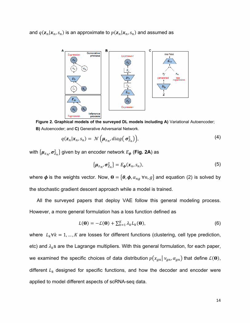
and R(3!|!!, 4!) is an approximate to '(3!|!!, 4!) and assumed as
R(3!|!!, 4!) = : TU0!, =VW6(X1!2 .Y, (4)
with ?U0!, X1!2 A given by an encoder network Z3 (Fig. 2A) as
?U0!, X1!2 A = Z3(!!, 4!), (5)
where [is the weights vector. Now, > = ?7,[, -!"∀%, 6A and equation (2) is solved by
the stochastic gradient descent approach while a model is trained.
All the surveyed papers that deploy VAE follow this general modeling process.
However, a more general formulation has a loss function defined as
\(>) = −ℒ(>) + ∑ ^4\4(>)/4)* , (6)
where \4∀_ = 1,… , a are losses for different functions (clustering, cell type prediction,
etc) and ^4s are the Lagrange multipliers. With this general formulation, for each paper,
we examined the specific choices of data distribution '()"!*+"!, -"!. that define ℒ(>),
different \4 designed for specific functions, and how the decoder and encoder were
applied to model different aspects of scRNA-seq data.
Figure 2. Graphical models of the surveyed DL models including A) Variational Autoencoder; B) Autoencoder; and C) Generative Adversarial Network.
15
3.2. Autoencoders
AEs learn the low dimensional latent representation 3! ∈ ℝ$ of expression !!. The AE
includes an encoder Z3 and a decoder /# (Fig. 2B) such that
3! = Z3(!!); !b! =/#(3!), (7)
where > = {7,[} are encoder and decoder weight parameters and !b! defines the
parameters (e.g. mean) of the likelihood '(!!|>) (Fig. 2B) and is often considered as
imputed and denoised expressions. Additional design can be included in the AE model
for batch correction, clustering, and other objectives.
The training of the AE is generally carried out by stochastic gradient descent
algorithms to minimize the loss similar to Eq. (6) except ℒ(>) = − log '(!!|>). When
'(!!|>) is the Gaussian, ℒ(>) becomes the mean square error (MSE) loss
ℒ(>) = ∑ ‖!! − !b!‖22(
!)* . (8)
Because different AE models differ in their AE architectures and the loss functions, we
will discuss the specific architecture and the loss functions for each reviewed DL model
in Section 4.
3.3. Generative adversarial networks
GANs have been used for imputation, data generation, and augmentation of the scRNA-
seq analysis. Without loss of generality, the GAN, when applied to scRNA-seq, is designed
to learn how to generate gene expression profiles from '5 , the distribution of !! . The
vanilla GAN consists of two deep neural networks [48]. The first network is the
generator"#(3!, e!) with parameter 7, a noise vector 3! from the distribution '0 and a
class label e (e.g. cell type) and is trained to generate !6, a "fake" gene expression (Fig.
16
2C). The second network is the discriminator network /3" with parameters [7, trained to
distinguish the "real" ! from fake !6 (Fig. 2C). Both networks, "# and /3" are trained to
outplay each other, resulting in a minimax game, in which "# is forced by /3" to produce
better samples, which, when converge, can fool the discriminator /3" , thus becoming
samples from '5 . The vanilla GAN suffers heavily from training instability and mode
collapsing[49]. To that end, Wasserstein GAN (WGAN) [49] was developed with the
WGAN loss [50]:
\(7) = maxø"
∑ /ø"(!!)(!)* − ∑ /ø"("9(3!, e!).
(!)* . (9)
Additional terms can also be added to equation (9) to constrain the functions of the
generator. Training based on the WGAN loss in Eq. (9) amounts to a min-max
optimization, which iterates between the discriminator and generator, where each
optimization is achieved by a stochastic gradient descent algorithm through
backpropagation. The WGAN requires/3" to be K-Lipschitz continuous [50], which can
be satisfied by adding the gradient penalty to the WGAN loss [49]. Once the training is
done, the generator "ø# can be used to generate gene expression profiles of new cells.
4. Survey of deep learning models for scRNA-seq analysis In this section, we survey applications of DL models for scRNA-seq analysis. To better
understand the relationship between the problems that each surveyed work addresses
and the key challenges in the general scRNA-seq processing pipeline, we divide the
survey into sections according to steps in the scRNA-seq processing pipeline illustrated
in Fig. 1. For each DL model, we present the model details under the general model

17
framework introduced in Section 3 and discuss the specific loss functions. We also survey
the evaluation metrics and summarize the evaluation results. To facilitate cross-
references of the information, we summarized all algorithms reviewed in this section in
Table 1 and tabulate the datasets and evaluation metrics used in each paper in Tables
2 & 3. We also listed all other algorithms that each surveyed method evaluated against
in Fig. 3, highlighting the extensiveness these algorithms were assessed for their
performance.
4.1. Imputation
4.1.1. DCA: deep count autoencoder
DCA [18] is an AE for imputation (Figs. 2B, 4B) and has been integrated into the Scanpy
framework.
Model. DCA models UMI counts with missing values using the ZINB distribution
'()"!|>. = f"!g(0) + (1 − f"!.hi(+"!, -"!., for 6 = 1,…"; % = 1,…h, (10)
where g(⋅) is a Dirac delta function,hi(⋅,⋅) denotes the negative binomial distribution,
and f"!, +"!, -"! , representing dropout rate, mean, and dispersion, respectively, are
functions of the output (!b!) of the decoder in the DCA as follows,
k! = 4V6lmV=(n:!b!);p! = exp(n;!b!) ; s! = exp(n<!b!), (11)
where n:, n;, and n< are additional weights to be estimated. The DCA encoder and
decoder follow the general AE formulation as in Eq. (7) but the encoder takes the
normalized, log-transformed expression as input. To train the model, DCA uses a
constrained log-likelihood as the loss function

18
\(>) = ∑ ∑ (−tm6'()"!|>. + ^f"!2 .=")*
(!)* , (12)
with > = {7,[,n: ,n;,n<}. Once the DCA is trained, the mean counts p! are used as
the denoised and imputed counts for cell %.
Results. For evaluation, DCA was compared to other methods using simulated data
(using Splatter R package), and real bulk transcriptomics data from a developmental C.
elegans time-course experiment was used with added simulating single-cell specific
noise. Gene expression was measured from 206 developmentally synchronized young
adults over a twelve-hour period (C. elegans). Single-cell specific noise was added in
silico by genewise subtracting values drawn from the exponential distribution such that
80% of values were zeros. The paper analyzed the Bulk contains less noise than single-
cell transcriptomics data and can thus aid in evaluating single-cell denoising methods by
providing a good ground truth model. The authors also did a comparison of other methods
including SAVER [36], scImpute [37], and MAGIC[51]. DCA denoising recovered original
time-course gene expression pattern while removing single-cell specific noise. Overall,
DCA demonstrated the strongest recovery of the top 500 genes most strongly associated
with development in the original data without noise; DCA was shown to outperform other
existing methods in capturing cell population structure in real data using PBMC, CITE-
seq, runtime scales linearly with the number of cells.
4.1.2. SAVER-X: single-cell analysis via expression recovery harnessing external data
SAVER-X [52] is an AE model (Figs. 2B, 4B) developed to denoise and impute scRNA-
seq data with transfer learning from other data resources.
19
Model. SAVER-X decomposes the variation in the observed counts !! with missing
values into three components: i) predictable structured component representing the
shared variation across genes, ii) unpredictable cell-level biological variation and gene-
specific dispersions, and iii) technical noise. Specifically, )"! is modeled as a Poisson-
Gamma hierarchical model,
'()"!|>. = umV44m%(t!)"!> ., '()"!> *+"!, -". = "WllW(+"!, -"+"!2 ., (13)
where t! is the sequencing depth of cell n, +"! is the mean, and -" is the dispersion. This
Poisson-Gamma mixture is an equivalent expression to the NB distribution and thus, the
ZINB distribution as Eq. (10) is adopted to model missing values.
The loss is similar to Eq. (12). However, +"! is initially learned by an AE pre-trained
using external datasets from an identical or similar tissue and then transferred to !! to be
denoised. Such transfer learning can be applied to data between species (e.g., human
and mouse in the study), cell types, batches, and single-cell profiling technologies. After
+"! is inferred, SAVER-X generates the final denoised data )v"! by an empirical Bayesian
shrinkage.
Results. SAVER-X was applied to multiple human single-cell datasets of different
scenarios: i) T-cell subtypes, ii) a cell type (CD4+ regulatory T cells) that was absent from
the pretraining dataset, iii) gene-protein correlations of CITE-seq data, and iv) immune
cells of primary breast cancer samples with a pretraining on normal immune cells.
SAVER-X with pretraining on HCA and/or PBMCs outperformed the same model without
pretraining and other denoising methods, including DCA [28], scVI[17], scImpute [37], and
MAGIC [51]. The model achieved promising results even for genes with very low UMI
counts. SAVER-X was also applied for a cross-species study in which the model was pre-
20
trained on a human or mouse dataset and transferred to denoise another. The results
demonstrated the merit of transferring public data resources to denoise in-house scRNA-
seq data even when the study species, cell types, or single-cell profiling technologies are
different.
4.1.3. DeepImpute: Deep neural network Imputation
DeepImpute [20] imputes genes in a divide-and-conquer approach, using a bank of DNN
models (Fig. 4A) with 512 output, each to predict gene expression levels of a cell.
Model. For each dataset, DeepImpute selects to impute a list of genes or highly variable
genes (variance over mean ratio, default = 0.5). Each sub-neural network aims to
understand the relationship between the input genes and a subset of target genes. Genes
are first divided into h random subsets of 512 target genes. For each subset, a two-layer
DNN is trained where the input includes genes that are among the top 5 best-correlated
genes to target genes but not part of the target genes in the subset. The loss is defined
as the weighted MSE
ℒ(>) = ∑!!(!! − !b!)2, (14)
which gives higher weights to genes with higher expression values.
Result. DeepImpute had the highest overall accuracy and offered shorter computation
time with less demand on computer memory than other methods like MAGIC, DrImpute,
ScImpute, SAVER, VIPER, and DCA. Using simulated and experimental datasets (Table
2), DeepImpute showed benefits in improving clustering results and identifying
significantly differentially expressed genes. DeepImpute and DCA, show overall
advantages over other methods and between which DeepImpute performs even better.
The properties of DeepImpute contribute to its superior performance include 1) a divide-
21
and-conquer approach which contrary to an autoencoder as implemented in DCA,
resulting in a lower complexity in each sub-model and stabilizing neural networks, and 2)
the subnetworks are trained without using the target genes as the input which reduces
overfitting while enforcing the network to understand true relationships between genes.
4.1.4. LATE: Learning with AuToEncoder
LATE [53] is an AE (Figs. 2B, 4B) whose encoder takes the log-transformed expression
as input.
Model. LATE sets zeros for all missing values and generates the imputed expressions.
LATE minimizes the MSE loss as Eq. (8). One issue is that some zeros could be real and
reflect the actual lack of expressions.
Result. Using synthetic data generated from pre-imputed data followed by random
dropout selection at different degrees, LATE outperforms other existing methods like
MAGIC, SAVER, DCA, scVI, particularly when the ground truth contains only a few or no
zeros. However, when the data contain many zero expression values, DCA achieved a
lower MSE than LATE, although LATE still has a smaller MSE than scVI. This result
suggests that DCA likely does a better job identifying true zero expressions, partly
because LATE does not make assumptions on the statistical distributions of the single-
cell data that potentially have inflated zero counts.
4.1.5. scGMAI
Technically, scGMAI [54] is a model for clustering but it includes an AE (Figs. 2B, 4B) in
the first step to combat dropout.
22
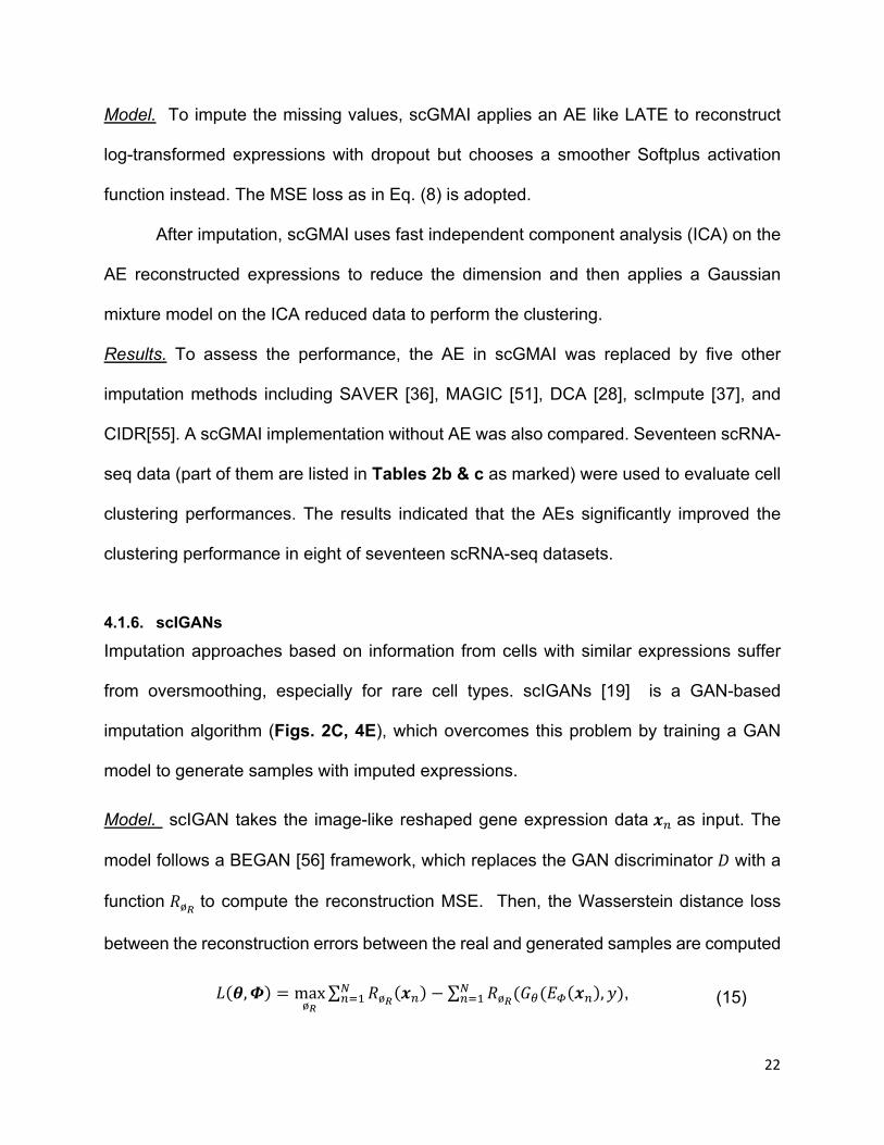
Model. To impute the missing values, scGMAI applies an AE like LATE to reconstruct
log-transformed expressions with dropout but chooses a smoother Softplus activation
function instead. The MSE loss as in Eq. (8) is adopted.
After imputation, scGMAI uses fast independent component analysis (ICA) on the
AE reconstructed expressions to reduce the dimension and then applies a Gaussian
mixture model on the ICA reduced data to perform the clustering.
Results. To assess the performance, the AE in scGMAI was replaced by five other
imputation methods including SAVER [36], MAGIC [51], DCA [28], scImpute [37], and
CIDR[55]. A scGMAI implementation without AE was also compared. Seventeen scRNA-
seq data (part of them are listed in Tables 2b & c as marked) were used to evaluate cell
clustering performances. The results indicated that the AEs significantly improved the
clustering performance in eight of seventeen scRNA-seq datasets.
4.1.6. scIGANs
Imputation approaches based on information from cells with similar expressions suffer
from oversmoothing, especially for rare cell types. scIGANs [19] is a GAN-based
imputation algorithm (Figs. 2C, 4E), which overcomes this problem by training a GAN
model to generate samples with imputed expressions.
Model. scIGAN takes the image-like reshaped gene expression data !! as input. The
model follows a BEGAN [56] framework, which replaces the GAN discriminator / with a
function wø$ to compute the reconstruction MSE. Then, the Wasserstein distance loss
between the reconstruction errors between the real and generated samples are computed
\(7,x) = maxø$
∑ wø$(!!)(!)* −∑ wø$("9(Z?(!!), e)
(!)* , (15)
23
This framework forces the model to meet two computing objectives, i.e. reconstructing the
real samples and discriminating between real and generated samples. Proportional
Control Theory was applied to balance these two goals during the training [57].
After training, the decoder "9 is used to generate new samples of a specific cell
type. Then, the k-nearest neighbors (KNN) approach is applied to the real and generated
samples to impute the real samples’ missing expressions.
Results. scIGANs was first tested on simulated samples with different dropout rates.
Performance of rescuing the correct clusters was compared with 11 existing imputation
approaches including DCA, DeepImpute, SAVER, scImpute, MAGIC, etc. scIGANs
reported the best performance for all metrics. scIGAN was next evaluated for its ability to
correctly cluster cell types on the Human brain scRNA-seq data, which showed superior
performance than existing methods again. scIGANs was then evaluated for identifying
cell-cycle states using scRNA-seq datasets from mouse embryonic stem cells. The
results showed that scIGANs outperformed competing existing approaches for recovering
subcellular states of cell cycle dynamics. scIGANs were further shown to improve the
identification of differentially expressed genes and enhance the inference of cellular
trajectory using time-course scRNA-seq data from the differentiation from H1 ESC to
definitive endoderm cells (DEC). Finally, scIGAN was also shown to scale to scRNA-seq
methods and data sizes.
4.2. Batch effect correction
4.2.1. BERMUDA: Batch Effect ReMoval Using Deep Autoencoders

24
BERMUDA [58] deploys a transfer-learning method (Figs. 2B, 4B) to remove the batch
effect. It performs correction to the shared cell clusters among batches and therefore
preserves batch-specific cell populations.
Model. BERMUDA is an AE that takes normalized, log-transformed expression as input.
Its consists of two parts as
\(>) = ℒ(>) + ^\%%@(>), (16)
where ℒ(>) is the MSE loss and \%%@ is the maximum mean discrepancy (MMD) [59]
loss that measures the differences in distributions between pairs of similar cell clusters
shared among batches as:
\%%@(>) = ∑ yA%,C%,A&,C&A%,A&,C%,C& yy/(3A%,C% , 3A&,C&), (17)
where 3A,C is the latent variable of !A,C, the input expression of a cell from cluster z of batch
V, yA%,C%,A&,C& is 1 if cluster VE of batch zE and cluster VF of batch zF are determined to be
similar by MetaNeighbor [60] and 0 , otherwise. The yy/ equals zero when the
underlying distributions of the observed samples are the same.
Results. BERMUDA was shown to outperform other methods like mnnCorrect [32],
BBKNN[61], Seurat [10], and scVI [17] in removing batch effects on simulated and human
pancreas data while preserving batch-specific biological signals. BERMUDA provides
several improvements compared to existing methods: 1) capable of removing batch
effects even when the cell population compositions across different batches are vastly
different; and 2) preserving batch-specific biological signals through transfer-learning
which enables discovering new information that might be hard to extract by analyzing
each batch individually.

25
4.2.2. DESC: batch correction based on clustering
DESC [62] is an AE model (Figs. 2B, 4B) that removes batch effect through clustering
with the hypothesis that batch differences in expressions are smaller than true biological
variations between cell types, and, therefore, properly performing clustering on cells
across multiple batches can remove batch effects without the need to define batches
explicitly.
Model. DESC has a conventional AE architecture. Its encoder takes normalized, log-
transformed expression and uses decoder output, !b! as the reconstructed gene
expression, which is equivalent to a Gaussian data distribution with !b! being the mean.
The loss function is similar to Eq. (16) and except that the second loss \G is the clustering
loss that regularizes the learned feature representations to form clusters as in the deep
embedded clustering [63]. The model is first trained to minimize ℒ(>) only to obtain the
initial weights before minimizing the combined loss. After the training, each cell is
assigned with a cluster ID.
Results. DESC was applied to the macaque retina dataset, which includes animal level,
region level, and sample-level batch effects. The results showed that DESC is effective
in removing the batch effect, whereas CCA [33], MNN [32], Seurat 3.0 [10], scVI [17],
BERMUDA [58], and scanorama [64] were all sensitive to batch definitions. DESC was
then applied to human pancreas datasets to test its ability to remove batch effects from
multiple scRNA-seq platforms and yielded the highest ARI among the comparing
approaches mentioned above. When applied to human PBMC data with interferon-beta
stimulation, where biological variations are compounded by batch effect, DESC was
shown to be the best in removing batch effect while preserving biological variations.

26
DESC was also shown to remove batch effect for the monocytes and mouse bone marrow
data and DESC was shown to preserve the pseudotemporal structure. Finally, DESC
scales linearly with the number of cells, and its running time is not affected by the
increasing number of batches.
4.2.3. iMAP: Integration of Multiple single-cell datasets by Adversarial Paired-style
transfer networks
iMAP [65] combines AE (Figs. 2B, 4B) and GAN (Figs. 2C, 4E) for batch effect removal.
It is designed to remove batch biases while preserving dataset-specific biological
variations.
Model. iMAP consists of two processing stages, each including a separate DL model. In
the first stage, a special AE, whose decoder combines the output of two separate
decoders /#'and /#(, is trained such that
3! = Z3(!!); !b! = /#(3!, 4!) = w{\|(/#'(4!) + /#((3!, 4!)), (18)
where 4! is the one-hot encoded batch number of cell %. /#' can be understood as
decoding the batch noise, whereas /#( reconstructs batch-removed expression from the
latent variable 3!. The training minimizes the loss in Eq. (16) except the 2nd loss is the
content loss
\H(>) = ∑ }3! − Z3(/#(3!, 4̃!).}22(
!)* , (19)
where 4̃! is a random batch number. Minimizing \H(>) further ensures the reconstructed
expression !b! would be batch agnostic and has the same content as !!.
However, due to the limitation of AE, this step is still insufficient for batch removal.
Therefore, a second stage is included to apply a GAN model to make expression
distributions of the shared cell type across different baches indistinguishable. To identified

27
the shared cell types, a mutual nearest neighbors (MNN) strategy adapted from [32] was
developed to identify MNN pairs across batches using batch effect independent 3! as
opposed to !!. Then, a mapping generator "## is trained using MNN pairs based on GAN
such that !!(J) = "##T!!
(L)Y, where !!(M) and !!
(J) are the MNN pairs from batch � and an
anchor batch Ä. The WGAN-GP loss as in Eq. (9) was adopted for the GAN training. After
training, "## is applied to all cells of a batch to generate batch-corrected expression.
Results: iMAP was first tested on benchmark datasets from human dendritic cells and
Jurkat and 293T cell lines and then human pancreas datasets from five different
platforms. All the datasets contain both batch-specific cells and batch-shared cell types.
iMAP was shown to separate the batch-specific cell types but mix batch shared cell types
and outperformed 9 other existing batch correction methods including Harmony, scVI,
fastMNN, Seurat, etc. iMAP was then applied to the large-scale Tabula Muris datasets
containing over 100K cells sequenced from two platforms. iMAP could not only reliably
integrate cells from the same tissues but identify cells from platform-specific tissues.
Finally, iMAP was applied to datasets of tumor-infiltrating immune cells and shown to
reduce the dropout ratio and the percentage of ribosomal genes and non-coding RNAs,
thus improving detection of rare cell types and ligand-receptor interactions. iMAP scales
with the number of cells, showing minimal time cost increase after the number of cells
exceeds thousands. Its performance is also robust against model hyperparameters.
4.3. Dimension reduction, latent representation, clustering, and data augmentation
4.3.1. Dimension reduction by AEs with gene-interaction constrained architecture
28
This study [66] considers AEs (Figs. 2B, 4B) for learning the low-dimensional
representation and specifically explores the benefit of incorporating prior biological
knowledge of gene-gene interactions to regularize the AE network architecture.
Model. Several AE models with single or two hidden layers that incorporate gene
interactions reflecting transcription factor (TF) regulations and protein-protein interactions
(PPIs) are implemented. The models take normalized, log-transformed expressions and
follow the general AE structure, including dimension-reducing and reconstructing layers,
but the network architectures are not symmetrical. Specifically, gene interactions are
incorporated such that each node of the first hidden layer represented a TF or a protein
in the PPI; only genes that are targeted by TFs or involved in the PPI were connected to
the node. Thus, the corresponding weights of Z3 and /# are set to be trainable and
otherwise fixed at zero throughout the training process. Both unsupervised (AE-like) and
supervised (cell-type label) learning were studied.
Results. Regularizing encoder connections with TF and PPI information considerably
reduced the model complexity by almost 90% (7.5-7.6M to 1.0-1.1M). The clusters formed
on the data representations learned from the models with or without TF and PPI
information were compared to those from PCA, NMF, independent component analysis
(ICA), t-SNE, and SIMLR [44]. The model with TF/PPI information and 2 hidden layers
achieved the best performance by five of the six measures and the best average
performance. In terms of the cell-type retrieval of single cells, the encoder models with
and without TF/PPI information achieved the best performance in 4 and 3 cell types,
respectively. PCA yielded the best performance in only 2 cell types. The DNN model with
TF/PPI information and 2 hidden layers again achieved the best average performance
29
across all cell types. In summary, this study demonstrated a biologically meaningful way
to regularize AEs by the prior biological knowledge for learning the representation of
scRNA-seq data for cell clustering and retrieval.
4.3.2. Dhaka: a VAE-based dimension reduction model.
Dhaka [67] was proposed to reduce the dimension of scRNA-seq data for efficient
stratification of tumor subpopulations.
Model. Dhaka adopts a general VAE formulation (Figs. 2A, 4C). It takes the normalized,
log-transformed expressions of a cell as input and outputs the low-dimensional
representation.
Result. Dhaka was first tested on the simulated dataset. The simulated dataset contains
500 cells, each including 3K genes, clustered into 5 different clusters with 100 cells each.
The clustering performance was compared with other methods including t-SNE, PCA,
SIMLR, NMF, an autoencoder, MAGIC, and scVI. Dhaka was shown to have an ARI
higher than most other comparing methods. Dhaka was then applied to the
Oligodendroglioma data and could separate malignant cells from non-malignant
microglia/macrophage cells. It also uncovered the shared glial lineage and differentially
expressed genes for the lineages. Dhaka was also applied to the Glioblastoma data and
revealed an evolutionary trajectory of the malignant cells where cells gradually evolve
from a stemlike state to a more differentiated state. In contrast, other methods failed to
capture this underlying structure. Dhaka was next applied to the Melanoma cancer
dataset [68] and uncovered two distinct clusters that showed the intra-tumor
heterogeneity of the Melanoma samples. Dhaka was finally applied to copy number
30
variation data [69] and shown to identify one major and one minor cell clusters, of which
other methods could not find.
4.3.3. scvis: a VAE for capturing low-dimensional structures
scvis [70] is a VAE network (Figs. 2A, 4C) that learns the low-dimensional
representations capture both local and global neighboring structures in scRNA-seq data.
Model: scvis adopts the generic VAE formulation described in section 3.1.However, it has
a unique loss function defined as
\(>) = −ℒ(>) + ^\H(>), (20)
where ℒ(>) is ELBO as in Eq. (3) and \H is a regularizer using non-symmetrized t-SNE
objective function [70], which is defined as
\H(>) = ∑ ∑ 'C|A logO)|++)|+
(C)*,CPA
(A)* , (21)
where V and z are two different cells, 'A|C measures the local cell relationship in the data
space, and RC|A measures such relationship in the latent space. Because t-SNE algorithm
preserves the local structure of high dimensional space, \H learns local structures of cells.
Results. scvis was tested on the simulated data and outperformed t-SNE in a nine-
dimensional space task. scvis preserved both local structure and global structure. The
relative positions of all clusters were well kept but outliers were scattered around clusters.
Using simulated data and comparing to t-SNE, scvis generally produced consistent and
better patterns among different runs while t-SNE could not. scvis also presented good
results on adding new data to an existing embedding, with median accuracy on new data
at 98.1% for K= 5 and 94.8% for K= 65, when train K cluster on original data then test the
classifier on new generated sample points. The scvis was subsequently tested on four
31
real datasets including metastatic melanoma, oligodendroglioma, mouse bipolar and
mouse retina datasets. In each dataset, scvis was showed to preserve both the global
and local structure of the data.
4.3.4. scVAE: VAE for single-cell gene expression data
scVAE [71] includes multiple VAE models (Figs. 2A, 4C) for denoising gene expression
levels and learning the low-dimensional latent representation of cells. It investigates
different choices of the likelihood functions in the VAE model to model different data sets.
Model. scVAE is a conventional fully connected network. However, different distributions
have been discussed for '()"!*+"!, -"!. to model different data behaviors. Specifically,
scVAE considers Poisson, constrained Poisson, and negative binomial distributions for
count data, piece-wise categorical Poisson for data including both high and low counts,
and zero-inflated version of these distributions to model missing values. To model
multiple modes in cell expressions, a Gaussian mixture is also considered for
R(3!|!!, 4!), resulting a GMVAE. The inference process still follows that of a VAE as
discussed in section 3.1.
Results. scVAEs were evaluated on the PBMC data and compared with factor analysis
(FA) models. The results showed that GMVAE with negative binomial distribution
achieved the highest lower bound and ARI. Zero-inflated Poisson distribution performed
the second best. All scVAE models outperformed the baseline linear factor analysis
model, which suggested that a non-linear model is needed to capture single-cell genomic
features. GMVAE was also compared with Seurat and shown to perform better using the
withheld data. However, scVAE performed no better than scVI [17] or scvis [70], both are
VAE models.
32
4.3.5. VASC: VAE for scRNA-seq
VASC [72] is another VAE (Figs. 2A, 4C) for dimension reduction and latent
representation but it models dropout.
Model: VASC’s input is the log-transformed expression but rescaled in the range [0,1]. A
dropout layer (dropout rate of 0.5) is added after the input layer to force subsequent layers
to learn to avoid dropout noise. The encoder network has three layers fully connected
and the first layer uses linear activation, which acts like an embedded PCA
transformation. The next two layers use the ReLU activation, which ensures a sparse and
stable output. This model's novelty is the zero-inflation layer (ZI layer), which is added
after the decoder to model scRNA-seq dropout events. The probability of dropout event
is defined as {Q5R(
where )v is the recovered expression value obtained by the decoder
network. Since backpropagation cannot deal with a stochastic network with categorical
variables, a Gumbel-softmax distribution [73] is introduced to address the difficulty of the
ZI layer. The loss function of the model takes the form \ = ℒ(>) + ^\/&(>), where ℒ is
the binary entropy because the input is scaled to [0 1], and\/& a loss performed using KL
divergence on the latent variables. After the model is trained, the latent code can be used
as the dimension-reduced feature for downstream tasks and visualization.
Results. VASC was compared with PCA, t-SNE, ZIFA, and SIMLR on 20 datasets. In the
study of embryonic development from zygote to blast cells, all methods roughly re-
established the development stages of different cell types in the dimension-reduced
space. However, VASC showed better performance to model embryo developmental
progression. In the Goolam, Biase and Yan datasets, scRNA-seq data were generated
through embryonic development stages from zygote to blast, VASC re-established
33
development stage from 1, 2, 4, 8, 16 to blast, while other methods failed. In the Pollen,
Kolodziejczyk, and Baron dataset, VASC formed an appropriate cluster, either with
homogeneous cell type, preserved proper relative positions, or minimal batch influence.
Interestingly, when tested on the PBMC dataset, VASC was showed to identify the major
global structure (B cells, CD4+, CD8+ T cells, NK cells, Dendritic cells), and detect subtle
differences within monocytes (FCGR3A+ vs CD14+ monocytes), indicating the capability
of VASC handling a large number of cells or cell types. Quantitative clustering
performance in NMI, ARI, homogeneity and completeness was also performed. VASC
always ranked top two in all the datasets. In terms of NMI and ARI, VASC best performed
on 15 and 17 out of 20 datasets, respectively.
4.3.6. scDeepCluster
scDeepCluster [74] is an AE network (Figs. 2B, 4B) that simultaneously learns feature
representation and performs clustering via explicit modeling of cell clusters as in DESC.
Model: Similar to DCA, scDeepCluster adopts a ZINB distribution for !!as in Eq. (10)
and (12).The loss is similar toEq. (16) but with the first being the negative log-likelihood
of the ZINB data distribution as defined in Eq. (12) and the second \G being a clustering
loss performed using KL divergence as in DESC algorithm. Compared to csvis,
scDeepcluster focuses more on clustering assignment due to the KL divergence.
Results. scDeepCluster was first tested on the simulation data and compared with other
seven methods including DCA [18], two multi-kernel spectral clustering methods MPSSC
[75] and SIMLR [44], CIDR [55], PCA + k-mean, scvis [70] and DEC[76]. In different
dropout rate simulations, scDeepCluster significantly outperformed the other methods
consistently. In signal strength, imbalanced sample size, and scalability simulations,

34
scDeepcluster outperformed all other algorithms and scDeepCluster and most notably
advantages for weak signals, robust against different data imbalance levels and scaled
linearly with the number of cells. scDeepCluster was then tested on four real datasets
(10X PBMC, Mouse ES cells, Mouse bladder cells, Worm neuron cells) and shown to
outperform all other comparing algorithms. Particularly, MPSSC and SIMLR failed to
process the full datasets due to quadratic complexity.
4.3.7. cscGAN: Conditional single-cell generative adversarial neural networks
cscGAN [77] is a GAN model (Figs. 2C, 4E) designed to augment the existing scRNA-
seq samples by generating expression profiles of specific cell types or subpopulations.
Model. Two models, csGAN and cscGAN, were developed following the general
formulation of WGAN described in section 3.3. The difference between the two models
is that cscGAN is a conditional GAN such that the input to the generator also includes a
class label e or cell type, i.e. [=(3, e) . The projection-based conditioning (PCGAN)
method [78] was adopted to obtain the conditional GAN. For both models, the generator
(three layers of 1024, 512, and 256 neurons) and discriminator (three layers of 256, 512,
and 1024 neurons) are fully connected DNNs.
Results: The performance of scGAN was first evaluated using PBMC data. The generated
samples were shown to capture the desired clusters and the real data's regulons.
Additionally, the AUC performance for classifying real from generated samples by a
Random Forest classifier only reached 0.65, performance close to 0.5. Finally, scGAN's
generated samples had a smaller MMD than those of Splatter, a state-of-the-art scRNA-
seq data simulator [79]. Even though a large MMD was observed for scGAN when
compared with that of SUGAR, another scRNA-seq simulator, SUGAR [80] was noted

35
for prohibitively high runtime and memory. scGAN was further trained and assessed on
the bigger mouse brain data and shown to model the expression dynamics across tissues.
Then, the performance of cscGAN for generating cell-type-specific samples was
evaluated using the PBMC data. cscGAN was shown to generate high-quality scRAN-
seq data for specific cell types. Finally, the real PBMC samples were augmented with the
generated samples. This augmentation improved the identification of rare cell types and
the ability to capture transitional cell states from trajectory analysis.
4.4. Multi-functional models
Given the versatility of AE and VAE in addressing different scRAN-seq analysis
challenges, DL models possessing multiple analysis functions have been developed. We
survey these models in this section.
4.4.1. scVI: single-cell variational inference
scVI [17] is designed to address a range of fundamental analysis tasks, including batch
correction, visualization, clustering, and differential expression.
Model. scVI is a VAE (Figs. 2A, 4C) that models the counts of each cell from different
batches. scVI adopts a ZINB distribution for )"!
'()"!*f"!, \!, +"!, -. = f"!g(0) + (1 − f"!.hi(\!+"!, -"., (22)
which is defined similarly as Eq (11) in DCA, except that \! denotes the scaling factor for
cell %, which follows a log-Normal (tm6:) prior as '(\!) = tm6:(Ç&! , É&!2 ., therefore, Ñ"!
represents the mean counts normalized by \!. Now, let 4! ∈ {0,1}S be the batch ID of cell
% with i being the total number of batches. Then, +"! and f" are further modeled as
36
functions of the =-dimension latent variable 3! ∈ ℝ$ and the batch ID 4! by the decoder
networks /#, and /#- as
0! = /#,(3!, 4!), k! = /#-(3!, 4!), (23)
where the 6th element of 0! and k! are +"!and f", respectively, and 7T , and 7: are the
decoder weights. Note that the lower layers of the two decoders are shared. For inference,
both 3! and \! are considered as latent variables and therefore R()!, 4!) =
R(3!|!!, 4!)R(\!|!!, 4!) is a mean-field approximate to the intractable posterior
distribution '(3!, \!|!!, 4!) and
R(3!|!!, 4!) = : TU0!, =VW6(X1!2 .Y,
R(\!|!!, 4!) = tm6: TU&!, =VW6(X&!2 .Y,
(24)
whose means and variances ?U0!, X1!2 A and ?U&!, X&!
2 A are defined by the encoder
networks Z1 and Z& applied to !! and 4! as
?U0!, X1!2 A = Z3.(!!, 4!),
?U&!, X&!2 A = Z3/(3!, 4!)
(25)
where [0 , and [& are the encoder weights. Note that, like the decoders, the lower layers
of the two encoders are also shared. Overall, the model parameters to be estimated by
the variational optimization is > = ?7T , 7: , [0 , [& , -"A. After inference, 3! are used for
visualization and clustering. +"! provides a batch-corrected, size-factor normalized
estimate of gene expression for each gene 6 in each cell %. An added advantage of the
probabilistic representation by scVI is that it provides a natural probabilistic treatment of
the subsequent differential analysis, resulting in lower variance in the adopted hypothesis
tests.
37
Results: scVI was evaluated for its scalability, the performance of imputation. For
scalability, ScVI was shown to be faster than most nonDL algorithms and scalable to
handle twice as many cells as nonDL algorithms with a fixed memory. For imputation,
ScVI, together with other ZINB-based models, performed better than methods using
alternative distributions. However, it underperformed for the dataset (HEMATO) with
fewer cells. For the latent space, scVI was shown to provide a comparable stratification
of cells into previously annotated cell types. Although scVI failed to ravel SIMLR, it is
among the best in capturing biological structures (hierarchical structure, dynamics, etc.)
and recognizing noise in data. For batch correction, it outperforms ComBat. For
normalizing sequencing depth, the size factor inferred by scVI was shown to be strongly
correlated with the sequencing depth. Interestingly, the negative binomial distribution in
the ZINB was found to explain the proportions of zero expressions in the cells, whereas
the zero probability f"! is found to be more correlated with alignment errors. For
differential expression analysis, scVI was shown to be among the best.
4.4.2. LDVAE: linearly decoded variational autoencoder
LDVAE [81] is an adaption of scVI to improve the model interpretability but it still benefits
from the scalability and efficiency of scVI. Also, this formulation applies to general VAE
models and thus is not restricted to scRNA-seq analysis.
Model. LDVAE follows scVI’s formulation but replaces the decoder /#, in Eq. (23) by a
linear model
0! = n3!, (26)
38
where n ∈ ℝ$×= is the weight matrix. Being the linear decoder provides interpretability in
the sense that the relationship between latent representation 3! and gene expression 0!
can be readily identified. LDVAE still follows the same loss and non-linear inference
scheme as scVI.
Results. LDVAE’s latent variable 3! could be used for clustering of cells with similar
accuracy as a VAE. Although LDVAE had a higher reconstruction error than VAE, due
to the linear decoder, the variations along the different axes of 3! establish direct linear
relationships with input genes. As an example from analyzing mouse embryo scRNA-seq,
Ö*,! , the second element of 3! , is shown to relate to simultaneous variations in the
expression of gene um|5á1 and à=6á1 . In contrast, such interpretability would be
intractable without approximation for a VAE. LDVAE was also shown to induce fewer
correlations between latent variables and to improve the grouping of the regulatory
programs. LDVAE is capable to scale to a large dataset with ~2M cells.
4.4.3. SAUCIE
SAUCIE [15] is an AE (Figs. 2B, 4B) designed to perform multiple functions, including
clustering, batch correlation, imputation, and visualization. SAUCIE is applied to the
normalized data instead of count data.
Model. SAUCIE includes multiple model components designed for different functions.
1. Clustering: SAUCIE first introduced a "digital" binary encoding layer âG ∈ {0,1}V in the
decoder / that functions to encode the cluster ID. To learn this encoding, an entropy
loss is introduced
\@ = ∑ '4 log '4/4)* , (27)

39
where '4 is the probability (proportion) of activation on neuron _ by the previous layer.
Minimizing this entropy loss promotes sparse neurons, thus forcing a binary encoding.
To encourage clustering behavior, SAUCIE also introduced an intracluster loss as
\W = ä }!bA − !bC}2
A,C:Y+0)Y)
0,
(28)
which computes the distance \W between the expressions of a pair of cells (!bA , !bC)
that have the same cluster ID (ℎAG = ℎC
G).
2. Batch correction: To correct the batch effect, an MMD loss is introduced to measure
the differences in terms of the distribution between batches in the latent space
\S = ∑ yy/(3Z[6 ,S\)*,\PZ[6 3\), (29)
where i is the total number of batches and 3Z[6 is the latent variable of an arbitrarily
chosen reference batch.
3. Imputation and visualization: The output of the decoder is taken by SAUCIE as an
imputed version of the input gene expression. To visualize the data without performing
an additional dimension reduction directly, the dimension of the latent variable 3! is
forced to 2.
Training the model includes two sequential runs. In the first run, an autoencoder is trained
to minimize the loss \] + ^S\S with \] being the MSE reconstruction loss defined in (9)
so that a batch-corrected, imputed input !å can be obtained at the output of the decoder.
In the second run, the bottleneck layer of the encoder from the first run is replaced by a
2-D latent code for visualization and a digital encoding layer is also introduced. This model
takes the cleaned !å as the input and is trained for clustering by minimizing the loss \] +
40
^@\@ + ^W\W . After the model is trained, )ç is the imputed, batch-corrected gene
expression. The 2-D latent code is used for visualization and the binary encoder encodes
the cluster ID.
Results. SAUCIE was evaluated for clustering, batch correction, imputation, and
visualization on both simulated and real scRNA-seq and scCyToF datasets. The
performance was compared to minibatch kmeans, Phenograph [82] and 22 for clustering;
MNN [32] and canonical correlation analysis (CCA) [33] for batch correction; PCA,
Monocle2 [83], diffusion maps, UMAP [84], tSNE [85] and PHATE [86] for visualization;
MAGIC [51], scImpute [37] and nearest neighbors completion (NN completion) for
imputation. Results showed that SAUCIE had a better or comparable performance with
other approaches. Also, SAUCIE has better scalability and faster runtimes than any of
the other models. SAUCIE's results on the scCyToF dengue dataset were further
analyzed in greater detail. SAUCIE was able to identify subtypes of the T cell populations
and demonstrated distinct cell manifold between acute and healthy subjects.
4.4.4. scScope:
scScope [87] is an AE (Figs. 2B, 4D) with recurrent steps designed for imputation and
batch correction.
Model. scScope has the following model design for batch correction and imputation.
1. Batch correction: A batch correction layer is applied to the input expression as
!!G = w{\|(!! − éèG), (30)
where and w{\ê is the ReLu activation function, é ∈ ℝ=×/ is the batch correction
matrix, èG ∈ {0,1}/×^is an indicator vector with entry 1 indicates the batch of the input,
and a is the total number of batches.
41
2. Recursive imputation: Instead of using the reconstructed expression !b!as the imputed
expression like in SAUCIE, scScope adds an imputer to !b! to recursively improve the
imputation result. The imputer is a single-layer autoencoder, whose decoder performs
the imputation as
!bC! = u_ë/_(3ví!.ì, (31)
where 3ví! is the output of the imputer encoder, /_ is the imputer decoder, and u_ is a
masking function that set the elements in !bC! that correspond to the non-missing
values to zero. Then, !bC! will be fed back to fill the missing value in the batch corrected
input as !!G + !bC!, which will be passed on to the main autoencoder. This recursive
imputation can iterate multiple cycles as selected.
The loss function is defined as
ℒ(>) =ä ä‖u_Q[!!G − !b!H ]‖
2
`
H)*
(
!)* (32)
where à is the total number of recursion, !b!H is the reconstructed expression at î th
recursion, u_Q is another masking function that forces the loss to compute only the non-
missing values in !!G .
Results. scScope was evaluated for its scalability, clustering, imputation, and batch
correction. It was compared with PCA, MAGIC, ZINB-WaVE, SIMLR, AE, scVI, and DCA.
For scalability and training speed, scScope was shown to offer scalability (for >100K cells)
with high efficiency (faster than most of the approaches). For clustering results, scScope
was shown to outperform most of the algorithms on small simulated datasets but offer
similar performance on large simulated datasets. For batch correction, scScope
performed comparably with other approaches but with faster runtime. For imputation,
42
scScope produced smaller errors consistently across a different range of expression.
scScope was further shown to be able to identify rear cell populations from a large mix of
cells.
4.5. Automated cell type identification
scRNA-seq is able to catalog cell types in complex tissues under different conditions.
However, the commonly adopted manual cell typing approach based on known markers
is time-consuming and less reproducible. We survey deep learning models of automated
cell type identification.
4.5.1. DigitalDLSorter
DigitalDLSorter [88] was proposed to identify and quantify the immune cells infiltrated in
tumors captured in bulk RNA-seq, utilizing single-cell RNA-seq data.
Model. DigitalDLSorter is a 4-layer DNN (Fig. 4A) (2 hidden layers of 200 neurons each
and an output of 10 cell types). The DigitalDLSorter is trained with two single-cell
datasets: breast cancers [89] and colorectal cancers [90]. For each cell, it is determined
to be tumor cell or non-tumor cell using RNA-seq based CNV method [89], followed by
using xCell algorithm [91] to determine immune cell types for non-tumor cells. Different
pseudo bulk (from 100 cells) RNA-seq datasets were prepared with known mixture
proportions to train the DNN. The output of DigitalDLSorter is the predicted proportions
of cell types in the input bulk sample.
Result. DigitalDLSorter was first tested on simulated bulk RNA-seq samples.
DigitalDLSorter achieved excellent agreement (linear correlation of 0.99 for colorectal
cancer, and good agreement in quadratic relationship for breast cancer) at predicting cell
43
types proportion. The proportion of immune and nonimmune cell subtypes of test bulk
TCGA samples was predicted by DigitalDLSorter and the results showed a very good
correlation to other deconvolution tools including TIMER [89], ESTIMATE [92], EPIC [93]
and MCPCounter [94]. Using DigitalDLSorter predicted CD8+ (good prognosis for overall
and disease-free survival) and Monocytes-Macrophages (MM, indicator for protumoral
activity) proportions, it is found that patients with higher CD8+/MM ratio had better survival
for both cancer types than those with lower CD8+/MM ratio. Both EPIC and MCPCounter
yielded non-significant survival associations using their cell proportion estimate.
4.5.2. scCapsNet
scCapsNet [95] is an interpretable capsule network designed for cell type prediction. The
paper showed that the trained network could be interpreted to inform marker genes and
regulatory modules of cell types.
Model. The two-layer architecture of scCapsNet takes log-transformed, normalized
expressions as input to form a feature extraction network (consists of \ parallel single-
layer neural networks) followed by a capsule network for cell-type classification (type
capsules). For each L parallel feature extraction layer, it generates a primary capsule è\ ∈
ℝ$1 as
è\ = w{\ê(na,\!!.∀t = 1,… , \ (33)
where na,\ ∈ ℝ$1×= is the weight matrix. Then, the primary capsules are fed into the
capsule network to compute a type capsules p4 ∈ ℝ$2, one for each cell type, as
p4 = 4R|W4ℎ ïäñ4\n4\è\
&
\
ó∀_ = 1,… , a (34)

44
where 4R|W4ℎ is the squashing function [96] to normalize the magnitude of its input vector
to be less than one, n4\ is another trainable weight matrix, and ñ4\ ∀t = 1,… , \ are the
coupling coefficients that represent the probability distribution of each primary capsule’s
impact on the prediction of cell type _ . ñ4\ is not trained but computed through the
dynamic routing process proposed in the original capsule networks [95]. The magnitude
of each type of capsule p4 represents the probability of a single cell !! belonging to cell
type _, which will be used for cell-type classification.
The training of the network minimizes the cross-entropy loss by the back-
propagation algorithm. Once trained, the interpretation of marker genes and regulatory
modules can be achieved by determining first the important primary capsules for each
cell type and then the most significant genes for each important primary capsule
(identified based on ñ4\ directly). To determine the genes that are important for an
important primary capsule t, genes are ranked base on the scores of the first principal
component computed from the columns of na,\ and then the markers are obtained by a
greedy search along with the ranked list for the best classification performance.
Results. scCapsNet’s performance was evaluated on human PBMCs [97] and mouse
retinal bipolar cells [98] datasets and shown to have comparable accuracies (99% and
97% respectively) with DNN and other popular ML algorithms (SVM, random forest, LDA
and nearest neighbor). However, the interpretability of scCapsNet was demonstrated
extensively. First, examining the coupling coefficients for each cell type showed that only
a few primary capsules have high values and thus are effective. Subsequently, a set of
core genes were identified for each effective capsule using the greedy search on the PC-
score ranked gene list. GO enrichment analysis showed that these core genes were
45
enriched in cell-type-related biological functions. Mapping the expression data into space
spanned by PCs of the columns of na,\ corresponding to all core genes uncovered
regulatory modules that would be missed by the T-SNE of gene expressions, which
demonstrated the effectiveness of the embeddings learned by scCapsNet in capturing
the functionally important features.
4.5.3. netAE: network-enhanced autoencoder
netAE [99] is a VAE-based semi-supervised cell type prediction model (Figs. 2A, 4C) that
deals with scenarios of having a small number of labeled cells.
Model. netAE works with UMI counts and assumes a ZINB distribution for )"! as in Eq.
(22) in scVI. However, netAE adopts the general VAE loss as in Eq. (6) with two function-
specific loss as
\(>) = −ℒ(>) + ^* ∑ ò(3!)!∈M + ^2∑ tm6á(e!|3!)!∈M/ , (35)
where � is a set of indices for all cells and �&is a subset of � for only cells with cell type
labels, ò is modified Newman and Girvan modularity [100] that quantifies cluster strength
using 3!, á is the softmax function, and e! is the cell type label. The second loss in Eq.
(34) functions as a clustering constraint and the last term is the cross-entropy loss that
constrains the cell type classification.
Results: netAE was compared with popular dimension reduction methods including scVI,
ZIFA, PCA and AE as well as a semi-supervised method scANVI [101]. For different
dimension reduction methods, cell type classification from latent features of cells was
carried out using KNN and logistic regression. The effect of different labeled samples
sizes on classification performance was also investigated, where the sample size varied
from as few as 10 cells to 70% of all cells. Among 3 test datasets (mouse brain cortex,
46
human embryo development, and mouse hematopoietic stem and progenitor cells),
netAE outperformed most of the baseline methods. Latent features were visualized using
t-SNE and cell clusters by netAE were tighter than those by other embedding spaces.
netAE also showed consistency of better cell-type classification with improved cell type
clustering. This suggested that the latent spaces learned with added modularity constraint
in the loss helped identify clusters of similar cells. Ablation study by removing each of the
three loss terms in Eq. (35) showed a drop of cell-type classification accuracy, suggesting
all three were necessary for the optimal performance.
4.5.4. scDGN - supervised adversarial alignment of single-cell RNA-seq data
scDGN [102], or Single Cell Domain Generalization Network (Fig. 4G), is an domain
adversarial network that aims to accurately assign cell types of single cells while
performing batch removal (domain adaptation) at the same time. It benefits from the
superior ability of domain adversarial learning to learn representations that are invariant
to technical confounders.
Model. scDGN takes the log-transformed, normalized expression as the input and has
three main modules: i) an encoder (Z3(!!)) for dimension reduction of scRNA-seq data,
ii) cell-type classifier, ô33 TZ3(!!)Y with parameters [W , and iii) domain (batch)
discriminator, /3" TZ3(!!)Y. The model has a Siamese design and the training takes a
pair of cells (!*, !2), each from the same or different batches. The encoder network
contains two hidden layers with 1146 and 100 neurons. ô33 classifies the cell type and
/3" predicts whether !* and !2 are from the same batch or not. The overall loss is
denoted by

47
\([,[W , [7) = \W öô33 TZ3(!*)Yõ − ^\@ ö/3" TZ3(!*)Y , /3" TZ3(!2)Yõ, (36)
where \W is the cross-entropy loss, \@ is a contrastive loss as described in [103]. Notice
that (46) has an adversarial formulation and minimizing this loss maximizes the
misclassification of cells from different batches, thus making them indistinguishable.
Similar to GAN training, scDGN is trained to iteratively solve: [C@ = argmin34\([C,[CW , [7.
and ([C,[CW. = argmin3,33\([,[W , [C@..
Results. scDGN was tested for classifying cell types and aligning batches ranging in size
from 10 to 39 cell types and from 4 to 155 batches. The performance was compared to a
series of deep learning and traditional machine learning methods, including Lin et al. DNN
[66], CaSTLe [104], MNN [32], scVI [17], and Seurat [10]. scDGN outperformed all other
methods in the classification accuracy on a subset of scQuery datasets (0.29), PBMC
(0.87), and 4 of the six Seurat pancreatic datasets (0.86-0.95). PCA visualization of the
learned data representations demonstrated that scDGN overcame the batch differences
and clearly separated cell clusters based on cell types, while other methods were
vulnerable to batch effects. In summary, scDGN is a supervised adversarial alignment
method to eliminate the batch effect of scRNA-seq data and create cleaner
representations of cell types.
4.6. Biological function prediction
Predicting biological function and response to treatment at single cell level or cell types
is critical to understand cellular system functioning and potent responses to stimulations.
DL models are capable of capture gene-gene relationship and their property in the latent
48
space. Several models we reviewed below provide exciting approaches to learn complex
biological functions and outcomes.
4.6.1. CNNC: convolutional neural network for coexpression
CNNC [105] is proposed to infer causal interactions between genes from scRNA-seq
data.
Model. CNNC is a Convolutional Neural Network (CNN) (Fig. 4F), the most popular DL
model. CNNC takes expression levels of two genes from many cells and transforms them
into a 32 x 32 image-like normalized empirical probability function (NEPDF), which
measures the probabilities of observing different coexpression levels between the two
genes. CNNC includes 6 convolutional layers, 3 max-pooling layers, 1 flatten layer, and
one output layer. All convolution layers have 32 kernels of size 3x3. Depending on the
application, the output layer can be designed to predict the state of interaction (Yes/No)
between the genes or the causal interaction between the input genes (no interaction,
gene A regulates gene B, or gene B regulates gene A).
Result. CNNC was trained to predict transcription factor (TF)-Gene interactions using the
mESC data from scQuery [106], where the ground truth interactions were obtained from
the ChIP-seq dataset from the GTRD database [107]. The performance was compared
with DNN, count statistics [108], and mutual information-based approach [109]. CNNC
was shown to have more than 20% higher AUPRC than other methods and reported
almost no false-negative for the top 5% predictions. CNNC was also trained to predict the
pathway regulator-target gene pairs. The positive regulator-gene pairs were obtained
from KEGG [110], Reactome [111], and negative samples were genes pairs that
appeared in pathways but not interacted. CNNC was shown to have better performance
49
of predicting regulator-gene pairs on both KEGG and Reactome pathways than other
methods including Pearson correlation, count statistics, GENIE3 [112], Mutual
information, Bayesian directed network (BDN), and DREMI [109]. CNNC was also
applied for causality prediction between two genes, that is if two genes regulate each
other and if they do, which gene is the regulator. The ground truth causal relationships
were also obtained from the KEGG and Reactome datasets. Again, CNNC reported better
performance than BDN, the common method developed to learn casual relationships from
gene expression data. CNNC was finally trained to assign 3 essential cell functions (cell
cycle, circadian rhythm, and immune system) to genes. This is achieved by training
CNNC to predict pairs of genes from the same function (e.g. Cell Cycle defined by
mSigDB from gene set enrichment analysis (GSEA) [113]) as 1 and all other pairs as 0.
The performance was compared with “guilt by association” and DNN, and CNNC was
shown to have more than 4% higher AUROC and reported all positives for the top 10%
predictions.
4.6.2. scGen, a generative model to predict perturbation response of single cells
across cell types
scGen [114] is designed to learn cell response to certain perturbation (drug treatment,
gene knockout, etc) from single cell expression data and predict the response to the same
perturbation for a new sample or a new cell type. The novelty of scGen is that it learns
the response in the latent space instead of the expression data space.
Model. ScGen follows the general VAE (Figs. 2A, 4C) for scRNA-seq data but uses the
“latent space arithmetics” to learn perturbations' response. Given scRNA-seq samples of
perturbed (denoted as p) and unperturbed cells (denoted as unp), a VAE model is trained.
50
Then, the latent space representation 3O and 3c!Oare obtained for the perturbed and
unperturbed cells. Following the notion that VAE could map nonlinear operations (e.g.,
perturbation) in the data space to linear operations in the latent space, ScGen estimate
the response in the latent space as û = 3üO − 3üc!O, where 3ü⋅ is the average representation
of samples from the same cell type or different cell types. Then, given the latent
representation 3>c!O of an unperturbed cell for a new sample from the same or different
cell type, the latent representation of the corresponding perturbed cell can be predicted
as 3>O=3>c!O + û. The expression of the perturbed cell can also be estimated by feeding
3>O into the VAE decoder. The scGen can also be expanded to samples and treatment
across two species (using orthologues between species). When scGen is trained for
species 1, or s1, with both perturbed and unperturbed cells but species 2, s2, with only
unperturbed cells, then the latent code for the perturbed cells from s2 can be predicted as
3L(,O =*
2(ÖL',O + ÖL(,c!O + gL + gO. where ûO = ÖL',c!O − ÖL',O captures the response of
perturbation and ûL = ÖL' − ÖL( represents the difference between species.
Result. scGen was applied to predict perturbation of out-of-samples response in human
PBMCs data, and scGen showed a higher average correlation (R2= 0.948) between
predicted and real data for six cell types. Comparing with other methods including CVAE
[115], style transfer GAN [116], linear approaches based on vector arithmetics(VA) [114]
and PCA+VA, scGen predicted full distribution of ISG15 gene (strongest regulated gene
by IFN-b) response to IFN- b [117], while others might predict mean (CAVE and style
transfer GAN) but failed to produce the full distribution. scGen was also tested on
predicting the intestinal epithelial cells’ response to infection[118]. For early transit-
amplifying cells, scGen showed good prediction (R2=0.98) for both H. poly and

51
Salmonella infection. Finally, scGen was evaluated for perturbation across species using
scRNA-seq data set by Hagai et al [119], which comprises bone marrow-derived
mononuclear phagocytes from mice, rats, rabbits, and pigs perturbed with
lipopolysaccharide (LPS). scGen’s predictions of LPS perturbation responses were
shown to be highly correlated (R2 = 0.91) with the real responses.
5. Conclusions
We systematically survey 25 DL models according to the challenges they address. Unlike
other surveys, we categorize major DL model statements into VAE, AE, and GAN with a
unified mathematic formulation in Section 3 (graphic model representation in Fig. 2),
which will guide readers to focus on the DL model selection, training strategies, and loss
functions in each algorithm. Specifically, the differences in loss functions are highlighted
in each DL model’s applications to meet specific objectives. DL/ML models that 25
surveyed models are evaluated against are presented in Fig. 3, providing a
straightforward way for readers to pick up the most suitable DL model at a specific step
for their own scRNA-seq data analysis. All evaluation methods are listed in Table 3, as
as we foresee to be an easy recipe book for researchers to establish their scRNA-seq
pipeline. In addition, a summary of all the 25 DL models concerning their DL models,
evaluation metrics, implementation environment, and downloadable source codes is
presented in Table 1. Taking together, this survey will provide a rich resource for DL
method selection for proper research applications, and we expect to inspire new DL
model development for scRNA-seq analysis.
52
In this review, we focus our survey on common DL models, such as AE, VAE, and
GAN, and their model variations or combinations to address single-cell data analysis
challenges. With the advancement of multi-omics single-cell technologies, such as cyTOF
(such as SAUCIE [15]), spatial transcriptome using DNN [120], and CITE-seq that
simultaneously generates read counts for surface protein expression along with gene
expression [121, 122]. Other than 3 most common DL models, we also include network
frameworks such as Capsule NN (such as scCapsNet [95]), Convolution NN (such as
CNNC [105]) and domain adaption learning (such as scDGN [102]). It is expected that
more DL models will be developed and implemented for the most challenging step for
scRNA-seq data, including but not limited to, data interpretation. For example, integrating
protein-protein interaction graphs into DL models has been shown for its advantages of
biological knowledge and nonlinear interactions embedded in the graphs [123-125].
Indeed, a recently published scRNA-seq analysis pipeline, scGNN [126], incorporates 3
iterative autoencoders (including one graph autoencoder) and successfully demonstrated
Alzheimer’s disease-related neural development and differentiation mechanism. We
expect that our careful organization of this review paper will provide a basic understanding
of DL models for scRNA-seq and a list of critical elements to be considered for future
developments in DLs.
Funding
This article's publication costs were supported partially by the National Institutes of Health
(CTSA 1UL1RR025767-01 to YC, R01GM113245 to YH, NCI Cancer Center Shared
Resources P30CA54174 to YC, and K99CA248944 to YCC); National Science
53
Foundation (2051113 to YFJ); Cancer Prevention and Research Institute of Texas
(RP160732 to YC, RP190346 to YC and YH); and the Fund for Innovation in Cancer
Informatics (ICI Fund to YCC and YC). The funding sources had no role in the design of
the study; collection, analysis, and interpretation of data; or in writing the manuscript.
Authors’ contributions
YH, YC, MF and YFJ conceived the study. MF, ZL, TZ, MMH, YCC, ZY, KP, SJ, JZ, SJG,
YFJ, YC and YH summarized resources, wrote, and approved the final version of paper.
References
1. Lahnemann D, Koster J, Szczurek E, McCarthy DJ, Hicks SC, Robinson MD, Vallejos CA,
Campbell KR, Beerenwinkel N, Mahfouz A et al: Eleven grand challenges in single-cell data
science. Genome Biol 2020, 21(1):31.
2. Vitak SA, Torkenczy KA, Rosenkrantz JL, Fields AJ, Christiansen L, Wong MH, Carbone L,
Steemers FJ, Adey A: Sequencing thousands of single-cell genomes with combinatorial
indexing. Nat Methods 2017, 14(3):302-308.
3. Wu H, Wang C, Wu S: Single-Cell Sequencing for Drug Discovery and Drug Development.
Curr Top Med Chem 2017, 17(15):1769-1777.
4. Kinker GS, Greenwald AC, Tal R, Orlova Z, Cuoco MS, McFarland JM, Warren A, Rodman
C, Roth JA, Bender SA et al: Pan-cancer single-cell RNA-seq identifies recurring programs
of cellular heterogeneity. Nat Genet 2020, 52(11):1208-1218.
5. Navin NE: The first five years of single-cell cancer genomics and beyond. Genome Res 2015, 25(10):1499-1507.
6. Suva ML, Tirosh I: Single-Cell RNA Sequencing in Cancer: Lessons Learned and Emerging
Challenges. Mol Cell 2019, 75(1):7-12.
7. Mannarapu M, Dariya B, Bandapalli OR: Application of single-cell sequencing technologies
in pancreatic cancer. Mol Cell Biochem 2021, 476(6):2429-2437.
8. Wauters E, Van Mol P, Garg AD, Jansen S, Van Herck Y, Vanderbeke L, Bassez A, Boeckx
B, Malengier-Devlies B, Timmerman A et al: Discriminating mild from critical COVID-19 by
innate and adaptive immune single-cell profiling of bronchoalveolar lavages. Cell Res 2021,
31(3):272-290.
9. Bost P, Giladi A, Liu Y, Bendjelal Y, Xu G, David E, Blecher-Gonen R, Cohen M, Medaglia
C, Li H et al: Host-Viral Infection Maps Reveal Signatures of Severe COVID-19 Patients.
Cell 2020, 181(7):1475-1488 e1412.
54
10. Stuart T, Butler A, Hoffman P, Hafemeister C, Papalexi E, Mauck WM, 3rd, Hao Y, Stoeckius
M, Smibert P, Satija R: Comprehensive Integration of Single-Cell Data. Cell 2019,
177(7):1888-1902 e1821.
11. Wolf FA, Angerer P, Theis FJ: SCANPY: large-scale single-cell gene expression data
analysis. Genome Biol 2018, 19(1):15.
12. Vaswani A, Shazeer N, Parmar N, Uszkoreit J, Jones L, Gomez AN, Kaiser Ł, Polosukhin I:
Attention is all you need. In: Advances in neural information processing systems: 2017.
5998-6008.
13. Karpathy A, Toderici G, Shetty S, Leung T, Sukthankar R, Fei-Fei L: Large-scale video
classification with convolutional neural networks. In: Proceedings of the IEEE conference on Computer Vision and Pattern Recognition: 2014. 1725-1732.
14. Deng L, Liu Y: Deep learning in natural language processing: Springer; 2018.
15. Amodio M, van Dijk D, Srinivasan K, Chen WS, Mohsen H, Moon KR, Campbell A, Zhao Y,
Wang X, Venkataswamy M et al: Exploring single-cell data with deep multitasking neural
networks. Nat Methods 2019, 16(11):1139-1145.
16. Srinivasan S, Leshchyk A, Johnson NT, Korkin D: A hybrid deep clustering approach for
robust cell type profiling using single-cell RNA-seq data. RNA 2020, 26(10):1303-1319.
17. Lopez R, Regier J, Cole MB, Jordan MI, Yosef N: Deep generative modeling for single-cell
transcriptomics. Nat Methods 2018, 15(12):1053-1058.
18. Eraslan G, Simon LM, Mircea M, Mueller NS, Theis FJ: Single-cell RNA-seq denoising using
a deep count autoencoder. Nat Commun 2019, 10(1):390.
19. Xu Y, Zhang Z, You L, Liu J, Fan Z, Zhou X: scIGANs: single-cell RNA-seq imputation using
generative adversarial networks. Nucleic Acids Res 2020, 48(15):e85.
20. Arisdakessian C, Poirion O, Yunits B, Zhu X, Garmire LX: DeepImpute: an accurate, fast,
and scalable deep neural network method to impute single-cell RNA-seq data. Genome Biol 2019, 20(1):211.
21. Tran HTN, Ang KS, Chevrier M, Zhang X, Lee NYS, Goh M, Chen J: A benchmark of batch-
effect correction methods for single-cell RNA sequencing data. Genome Biol 2020, 21(1):12.
22. Petegrosso R, Li Z, Kuang R: Machine learning and statistical methods for clustering single-
cell RNA-sequencing data. Brief Bioinform 2020, 21(4):1209-1223.
23. Abdelaal T, Michielsen L, Cats D, Hoogduin D, Mei H, Reinders MJT, Mahfouz A: A
comparison of automatic cell identification methods for single-cell RNA sequencing data.
Genome Biol 2019, 20(1):194.
24. Wang J, Zou Q, Lin C: A comparison of deep learning-based pre-processing and clustering
approaches for single-cell RNA sequencing data. Briefings in Bioinformatics 2021.
25. Picelli S, Bjorklund AK, Faridani OR, Sagasser S, Winberg G, Sandberg R: Smart-seq2 for
sensitive full-length transcriptome profiling in single cells. Nat Methods 2013, 10(11):1096-
1098.
26. Macosko EZ, Basu A, Satija R, Nemesh J, Shekhar K, Goldman M, Tirosh I, Bialas AR,
Kamitaki N, Martersteck EM et al: Highly Parallel Genome-wide Expression Profiling of
Individual Cells Using Nanoliter Droplets. Cell 2015, 161(5):1202-1214.
27. Eisenstein M: Single-cell RNA-seq analysis software providers scramble to offer solutions.
Nat Biotechnol 2020, 38(3):254-257.
55
28. Chen G, Ning B, Shi T: Single-Cell RNA-Seq Technologies and Related Computational Data
Analysis. Front Genet 2019, 10:317.
29. Vallejos CA, Marioni JC, Richardson S: BASiCS: Bayesian Analysis of Single-Cell
Sequencing Data. PLoS Comput Biol 2015, 11(6):e1004333.
30. Lun AT, Bach K, Marioni JC: Pooling across cells to normalize single-cell RNA sequencing
data with many zero counts. Genome Biol 2016, 17:75.
31. Hafemeister C, Satija R: Normalization and variance stabilization of single-cell RNA-seq
data using regularized negative binomial regression. Genome Biol 2019, 20(1):296.
32. Haghverdi L, Lun ATL, Morgan MD, Marioni JC: Batch effects in single-cell RNA-sequencing
data are corrected by matching mutual nearest neighbors. Nat Biotechnol 2018, 36(5):421-
427.
33. Butler A, Hoffman P, Smibert P, Papalexi E, Satija R: Integrating single-cell transcriptomic
data across different conditions, technologies, and species. Nat Biotechnol 2018, 36(5):411-
420.
34. Korsunsky I, Millard N, Fan J, Slowikowski K, Zhang F, Wei K, Baglaenko Y, Brenner M,
Loh PR, Raychaudhuri S: Fast, sensitive and accurate integration of single-cell data with
Harmony. Nat Methods 2019, 16(12):1289-1296.
35. Peng T, Zhu Q, Yin P, Tan K: SCRABBLE: single-cell RNA-seq imputation constrained by
bulk RNA-seq data. Genome Biol 2019, 20(1):88.
36. Huang M, Wang J, Torre E, Dueck H, Shaffer S, Bonasio R, Murray JI, Raj A, Li M, Zhang
NR: SAVER: gene expression recovery for single-cell RNA sequencing. Nat Methods 2018,
15(7):539-542.
37. Li WV, Li JJ: An accurate and robust imputation method scImpute for single-cell RNA-seq
data. Nat Commun 2018, 9(1):997.
38. Roweis ST, Saul LK: Nonlinear dimensionality reduction by locally linear embedding.
Science 2000, 290(5500):2323-2326.
39. Welch JD, Hartemink AJ, Prins JF: SLICER: inferring branched, nonlinear cellular
trajectories from single cell RNA-seq data. Genome Biol 2016, 17(1):106.
40. Linderman GC, Rachh M, Hoskins JG, Steinerberger S, Kluger Y: Fast interpolation-based
t-SNE for improved visualization of single-cell RNA-seq data. Nat Methods 2019, 16(3):243-
245.
41. Becht E, McInnes L, Healy J, Dutertre CA, Kwok IWH, Ng LG, Ginhoux F, Newell EW:
Dimensionality reduction for visualizing single-cell data using UMAP. Nat Biotechnol 2018.
42. Subelj L, Bajec M: Unfolding communities in large complex networks: combining defensive
and offensive label propagation for core extraction. Phys Rev E Stat Nonlin Soft Matter Phys 2011, 83(3 Pt 2):036103.
43. Traag VA, Waltman L, van Eck NJ: From Louvain to Leiden: guaranteeing well-connected
communities. Sci Rep 2019, 9(1):5233.
44. Wang B, Zhu J, Pierson E, Ramazzotti D, Batzoglou S: Visualization and analysis of single-
cell RNA-seq data by kernel-based similarity learning. Nat Methods 2017, 14(4):414-416.
45. Finak G, McDavid A, Yajima M, Deng J, Gersuk V, Shalek AK, Slichter CK, Miller HW,
McElrath MJ, Prlic M et al: MAST: a flexible statistical framework for assessing
56
transcriptional changes and characterizing heterogeneity in single-cell RNA sequencing
data. Genome Biol 2015, 16:278.
46. Kharchenko PV, Silberstein L, Scadden DT: Bayesian approach to single-cell differential
expression analysis. Nat Methods 2014, 11(7):740-742.
47. Miao Z, Deng K, Wang X, Zhang X: DEsingle for detecting three types of differential
expression in single-cell RNA-seq data. Bioinformatics 2018, 34(18):3223-3224.
48. Goodfellow I, Pouget-Abadie J, Mirza M, Xu B, Warde-Farley D, Ozair S, Courville A, Bengio
Y: Generative adversarial networks. Communications of the ACM 2020, 63(11):139-144.
49. Gulrajani I, Ahmed F, Arjovsky M, Dumoulin V, Courville A: Improved training of wasserstein
gans. arXiv preprint arXiv:170400028 2017.
50. Arjovsky M, Chintala S, Bottou L: Wasserstein gan. arXiv 2017. arXiv preprint arXiv:170107875 2017, 30.
51. van Dijk D, Sharma R, Nainys J, Yim K, Kathail P, Carr AJ, Burdziak C, Moon KR, Chaffer
CL, Pattabiraman D et al: Recovering Gene Interactions from Single-Cell Data Using Data
Diffusion. Cell 2018, 174(3):716-729 e727.
52. Wang J, Agarwal D, Huang M, Hu G, Zhou Z, Ye C, Zhang NR: Data denoising with transfer
learning in single-cell transcriptomics. Nat Methods 2019, 16(9):875-878.
53. Badsha MB, Li R, Liu B, Li YI, Xian M, Banovich NE, Fu AQ: Imputation of single-cell gene
expression with an autoencoder neural network. Quant Biol 2020, 8(1):78-94.
54. Yu B, Chen C, Qi R, Zheng R, Skillman-Lawrence PJ, Wang X, Ma A, Gu H: scGMAI: a
Gaussian mixture model for clustering single-cell RNA-Seq data based on deep
autoencoder. Brief Bioinform 2020.
55. Lin P, Troup M, Ho JW: CIDR: Ultrafast and accurate clustering through imputation for
single-cell RNA-seq data. Genome Biol 2017, 18(1):59.
56. Berthelot D, Schumm, T. and Metz, L.: BEGAN: Boundary Equilibrium Generative
Adversarial Networks. arXiv 2017.
57. Berthelot D, Schumm T, Metz L: Began: Boundary equilibrium generative adversarial
networks. arXiv preprint arXiv:170310717 2017.
58. Wang T, Johnson TS, Shao W, Lu Z, Helm BR, Zhang J, Huang K: BERMUDA: a novel
deep transfer learning method for single-cell RNA sequencing batch correction reveals
hidden high-resolution cellular subtypes. Genome Biol 2019, 20(1):165.
59. Borgwardt KM, Gretton A, Rasch MJ, Kriegel HP, Scholkopf B, Smola AJ: Integrating
structured biological data by Kernel Maximum Mean Discrepancy. Bioinformatics 2006,
22(14):e49-57.
60. Crow M, Paul A, Ballouz S, Huang ZJ, Gillis J: Characterizing the replicability of cell types
defined by single cell RNA-sequencing data using MetaNeighbor. Nat Commun 2018,
9(1):884.
61. Polanski K, Young MD, Miao Z, Meyer KB, Teichmann SA, Park JE: BBKNN: fast batch
alignment of single cell transcriptomes. Bioinformatics 2020, 36(3):964-965.
62. Li X, Wang K, Lyu Y, Pan H, Zhang J, Stambolian D, Susztak K, Reilly MP, Hu G, Li M:
Deep learning enables accurate clustering with batch effect removal in single-cell RNA-seq
analysis. Nat Commun 2020, 11(1):2338.

57
63. Guo X, Gao, L., Liu, X., and Yin, J.: Improved deep embedded clustering with local structure
preservation. Proc 26th International Joint Conference on Artificial Integlligence 2017:1753-
1759.
64. Hie B, Bryson B, Berger B: Efficient integration of heterogeneous single-cell transcriptomes
using Scanorama. Nat Biotechnol 2019, 37(6):685-691.
65. Wang D, Hou S, Zhang L, Wang X, Liu B, Zhang Z: iMAP: integration of multiple single-cell
datasets by adversarial paired transfer networks. Genome Biol 2021, 22(1):63.
66. Lin C, Jain S, Kim H, Bar-Joseph Z: Using neural networks for reducing the dimensions of
single-cell RNA-Seq data. Nucleic Acids Res 2017, 45(17):e156.
67. Rashid S, Shah S, Bar-Joseph Z, Pandya R: Dhaka: Variational Autoencoder for Unmasking
Tumor Heterogeneity from Single Cell Genomic Data. Bioinformatics 2019.
68. Tirosh I, Izar B, Prakadan SM, Wadsworth MH, 2nd, Treacy D, Trombetta JJ, Rotem A,
Rodman C, Lian C, Murphy G et al: Dissecting the multicellular ecosystem of metastatic
melanoma by single-cell RNA-seq. Science 2016, 352(6282):189-196.
69. Zahn H, Steif A, Laks E, Eirew P, VanInsberghe M, Shah SP, Aparicio S, Hansen CL:
Scalable whole-genome single-cell library preparation without preamplification. Nature Methods 2017, 14(2):167-173.
70. Ding J, Condon A, Shah SP: Interpretable dimensionality reduction of single cell
transcriptome data with deep generative models. Nat Commun 2018, 9(1):2002.
71. Gronbech CH, Vording MF, Timshel PN, Sonderby CK, Pers TH, Winther O: scVAE:
variational auto-encoders for single-cell gene expression data. Bioinformatics 2020,
36(16):4415-4422.
72. Wang D, Gu J: VASC: Dimension Reduction and Visualization of Single-cell RNA-seq Data
by Deep Variational Autoencoder. Genomics Proteomics Bioinformatics 2018, 16(5):320-
331.
73. Jang E. GSaPB: Categorical reparameterization with gumbel-softmax. arXiv 2016.
74. Tian T, Wan, J., Song, Q. et al.: Clustering single-cell RNA-seq data with a model-based
deep learning approach. Nat Mach Intell 2019, 1.
75. Regev A, Teichmann SA, Lander ES, Amit I, Benoist C, Birney E, Bodenmiller B, Campbell
P, Carninci P, Clatworthy M et al: The Human Cell Atlas. Elife 2017, 6.
76. Xie J, Girshick R, Farhadi A: Unsupervised deep embedding for clustering analysis. In:
International conference on machine learning: 2016. PMLR: 478-487.
77. Marouf M, Machart P, Bansal V, Kilian C, Magruder DS, Krebs CF, Bonn S: Realistic in silico
generation and augmentation of single-cell RNA-seq data using generative adversarial
networks. Nat Commun 2020, 11(1):166.
78. Miyato TaK, M: cGANs with projection discriminator. Preprint 2018.
79. Zappia L, Phipson B, Oshlack A: Splatter: simulation of single-cell RNA sequencing data.
Genome Biol 2017, 18(1):174.
80. Lindenbaum O, Stanley, J. S., Wolf, G. and Krishnaswamy, S. : Geometry-based data
generation. Advances in Neural Information Processing Systems 2018.
81. Svensson V, Gayoso A, Yosef N, Pachter L: Interpretable factor models of single-cell RNA-
seq via variational autoencoders. Bioinformatics 2020, 36(11):3418-3421.
58
82. Levine JH, Simonds EF, Bendall SC, Davis KL, Amir el AD, Tadmor MD, Litvin O, Fienberg
HG, Jager A, Zunder ER et al: Data-Driven Phenotypic Dissection of AML Reveals
Progenitor-like Cells that Correlate with Prognosis. Cell 2015, 162(1):184-197.
83. Qiu X, Mao Q, Tang Y, Wang L, Chawla R, Pliner HA, Trapnell C: Reversed graph
embedding resolves complex single-cell trajectories. Nat Methods 2017, 14(10):979-982.
84. McInnes L, Healy, J. & Melville, J.: Umap: uniform manifold approximation and projection
for dimension reduction. ArXiv 2018.
85. van der Maaten LH, G.: Visualizing data using t-SNE. J Mach Learn 2008, 9:2579-2605.
86. Moon KRea: PHATE: a dimensionality reduction method for visualizing trajectory structures
in high-dimensional biological data. bioRxiv 2017.
87. Deng Y, Bao F, Dai Q, Wu LF, Altschuler SJ: Scalable analysis of cell-type composition from
single-cell transcriptomics using deep recurrent learning. Nat Methods 2019, 16(4):311-314.
88. Torroja C, Sanchez-Cabo F: Digitaldlsorter: Deep-Learning on scRNA-Seq to Deconvolute
Gene Expression Data. Front Genet 2019, 10:978.
89. Chung W, Eum HH, Lee HO, Lee KM, Lee HB, Kim KT, Ryu HS, Kim S, Lee JE, Park YH et al: Single-cell RNA-seq enables comprehensive tumour and immune cell profiling in
primary breast cancer. Nat Commun 2017, 8:15081.
90. Li H, Courtois ET, Sengupta D, Tan Y, Chen KH, Goh JJL, Kong SL, Chua C, Hon LK, Tan
WS et al: Reference component analysis of single-cell transcriptomes elucidates cellular
heterogeneity in human colorectal tumors. Nat Genet 2017, 49(5):708-718.
91. Aran D, Hu Z, Butte AJ: xCell: digitally portraying the tissue cellular heterogeneity landscape.
Genome Biol 2017, 18(1):220.
92. Yoshihara K, Shahmoradgoli M, Martinez E, Vegesna R, Kim H, Torres-Garcia W, Trevino
V, Shen H, Laird PW, Levine DA et al: Inferring tumour purity and stromal and immune cell
admixture from expression data. Nat Commun 2013, 4:2612.
93. Racle J, de Jonge K, Baumgaertner P, Speiser DE, Gfeller D: Simultaneous enumeration of
cancer and immune cell types from bulk tumor gene expression data. Elife 2017, 6.
94. Becht E, Giraldo NA, Lacroix L, Buttard B, Elarouci N, Petitprez F, Selves J, Laurent-Puig
P, Sautes-Fridman C, Fridman WH et al: Estimating the population abundance of tissue-
infiltrating immune and stromal cell populations using gene expression. Genome Biol 2016,
17(1):218.
95. Wang L, Nie, R., Yu, Z. et al.: An interpretable deep-learning architecture of capsule
networks for identifying cell-type gene expression programs from single-cell RNA-
sequencing data. Nat Mach Intell 2020, 2:693-703.
96. Patel ND, Nguang SK, Coghill GG: Neural network implementation using bit streams. IEEE Trans Neural Netw 2007, 18(5):1488-1504.
97. Zheng GX, Terry JM, Belgrader P, Ryvkin P, Bent ZW, Wilson R, Ziraldo SB, Wheeler TD,
McDermott GP, Zhu J et al: Massively parallel digital transcriptional profiling of single cells.
Nat Commun 2017, 8:14049.
98. Shekhar K, Lapan SW, Whitney IE, Tran NM, Macosko EZ, Kowalczyk M, Adiconis X, Levin
JZ, Nemesh J, Goldman M et al: Comprehensive Classification of Retinal Bipolar Neurons
by Single-Cell Transcriptomics. Cell 2016, 166(5):1308-1323 e1330.
59
99. Dong Z, Alterovitz G: netAE: semi-supervised dimensionality reduction of single-cell RNA
sequencing to facilitate cell labeling. Bioinformatics 2021, 37(1):43-49.
100. Newman ME: Modularity and community structure in networks. Proc Natl Acad Sci U S A 2006, 103(23):8577-8582.
101. Xu C, Lopez R, Mehlman E, Regier J, Jordan MI, Yosef N: Probabilistic harmonization and
annotation of single-cell transcriptomics data with deep generative models. Mol Syst Biol 2021, 17(1):e9620.
102. Ge S, Wang H, Alavi A, Xing E, Bar-Joseph Z: Supervised Adversarial Alignment of Single-
Cell RNA-seq Data. J Comput Biol 2021, 28(5):501-513.
103. Hadsell R, Chopra S, LeCun Y: Dimensionality reduction by learning an invariant mapping.
In: 2006 IEEE Computer Society Conference on Computer Vision and Pattern Recognition (CVPR'06): 2006. IEEE: 1735-1742.
104. Lieberman Y, Rokach L, Shay T: CaSTLe–classification of single cells by transfer learning:
harnessing the power of publicly available single cell RNA sequencing experiments to
annotate new experiments. PloS one 2018, 13(10):e0205499.
105. Yuan Y, Bar-Joseph Z: Deep learning for inferring gene relationships from single-cell
expression data. Proc Natl Acad Sci U S A 2019.
106. Alavi A, Ruffalo M, Parvangada A, Huang Z, Bar-Joseph Z: A web server for comparative
analysis of single-cell RNA-seq data. Nat Commun 2018, 9(1):4768.
107. Yevshin I, Sharipov R, Valeev T, Kel A, Kolpakov F: GTRD: a database of transcription
factor binding sites identified by ChIP-seq experiments. Nucleic Acids Research 2016,
45(D1):D61-D67.
108. Wang YXR, Waterman MS, Huang HY: Gene coexpression measures in large
heterogeneous samples using count statistics. P Natl Acad Sci USA 2014, 111(46):16371-
16376.
109. Krishnaswamy S, Spitzer MH, Mingueneau M, Bendall SC, Litvin O, Stone E, Pe'er D, Nolan
GP: Systems biology. Conditional density-based analysis of T cell signaling in single-cell
data. Science 2014, 346(6213):1250689.
110. Kanehisa M, Furumichi M, Tanabe M, Sato Y, Morishima K: KEGG: new perspectives on
genomes, pathways, diseases and drugs. Nucleic Acids Res 2017, 45(D1):D353-D361.
111. Fabregat A, Jupe S, Matthews L, Sidiropoulos K, Gillespie M, Garapati P, Haw R, Jassal B,
Korninger F, May B et al: The Reactome Pathway Knowledgebase. Nucleic Acids Res 2018,
46(D1):D649-D655.
112. Huynh-Thu VA, Irrthum A, Wehenkel L, Geurts P: Inferring regulatory networks from
expression data using tree-based methods. PloS one 2010, 5(9):e12776.
113. Subramanian A, Tamayo P, Mootha VK, Mukherjee S, Ebert BL, Gillette MA, Paulovich A,
Pomeroy SL, Golub TR, Lander ES et al: Gene set enrichment analysis: a knowledge-based
approach for interpreting genome-wide expression profiles. Proc Natl Acad Sci U S A 2005,
102(43):15545-15550.
114. Lotfollahi M, Wolf FA, Theis FJ: scGen predicts single-cell perturbation responses. Nat Methods 2019, 16(8):715-721.

60
115. Duvenaud D, Maclaurin D, Iparraguirre J, Bombarell R, Hirzel T, Aspuru-Guzik A, Adams R:
Advances in Neural Information Processing Systems 28. Cortes C, Lawrence ND, Lee DD, Sugiyama M, Garnett R, Eds 2015:2224-2232.
116. Amodio M, Krishnaswamy S: MAGAN: Aligning biological manifolds. In: International Conference on Machine Learning: 2018. PMLR: 215-223.
117. Kang HM, Subramaniam M, Targ S, Nguyen M, Maliskova L, McCarthy E, Wan E, Wong S,
Byrnes L, Lanata CM et al: Multiplexed droplet single-cell RNA-sequencing using natural
genetic variation. Nat Biotechnol 2018, 36(1):89-94.
118. Haber AL, Biton M, Rogel N, Herbst RH, Shekhar K, Smillie C, Burgin G, Delorey TM, Howitt
MR, Katz Y et al: A single-cell survey of the small intestinal epithelium. Nature 2017,
551(7680):333-339.
119. Hagai T, Chen X, Miragaia RJ, Rostom R, Gomes T, Kunowska N, Henriksson J, Park JE,
Proserpio V, Donati G et al: Gene expression variability across cells and species shapes
innate immunity. Nature 2018, 563(7730):197-202.
120. Maseda F, Cang Z, Nie Q: DEEPsc: A Deep Learning-Based Map Connecting Single-Cell
Transcriptomics and Spatial Imaging Data. Front Genet 2021, 12:636743.
121. Musu Y, Liang C, Deng M: Clustering single cell CITE-seq data with a canonical correlation
based deep learning method. bioRxiv 2021.
122. Zhou Z, Ye C, Wang J, Zhang NR: Surface protein imputation from single cell transcriptomes
by deep neural networks. Nat Commun 2020, 11(1):651.
123. Ramirez R, Chiu Y-C, Hererra A, Mostavi M, Ramirez J, Chen Y, Huang Y, Jin Y-F:
Classification of Cancer Types Using Graph Convolutional Neural Networks. Frontiers in Physics 2020, 8(203).
124. Ramirez R, Chiu YC, Zhang S, Ramirez J, Chen Y, Huang Y, Jin YF: Prediction and
interpretation of cancer survival using graph convolution neural networks. Methods 2021,
192:120-130.
125. Battaglia PW, Hamrick JB, Bapst V, Sanchez-Gonzalez A, Zambaldi V, Malinowski M,
Tacchetti A, Raposo D, Santoro A, Faulkner R: Relational inductive biases, deep learning,
and graph networks. arXiv preprint arXiv:180601261 2018.
126. Wang J, Ma A, Chang Y, Gong J, Jiang Y, Qi R, Wang C, Fu H, Ma Q, Xu D: scGNN is a
novel graph neural network framework for single-cell RNA-Seq analyses. Nat Commun 2021,
12(1):1882.
127. Peng Y, Baulier E, Ke Y, Young A, Ahmedli NB, Schwartz SD, Farber DB: Human embryonic
stem cells extracellular vesicles and their effects on immortalized human retinal Muller cells.
PLoS One 2018, 13(3):e0194004.
128. Stoeckius M, Hafemeister C, Stephenson W, Houck-Loomis B, Chattopadhyay PK,
Swerdlow H, Satija R, Smibert P: Simultaneous epitope and transcriptome measurement in
single cells. Nat Methods 2017, 14(9):865-868.
129. La Manno G, Gyllborg D, Codeluppi S, Nishimura K, Salto C, Zeisel A, Borm LE, Stott SRW,
Toledo EM, Villaescusa JC et al: Molecular Diversity of Midbrain Development in Mouse,
Human, and Stem Cells. Cell 2016, 167(2):566-580 e519.
130. Azizi E, Carr AJ, Plitas G, Cornish AE, Konopacki C, Prabhakaran S, Nainys J, Wu K,
Kiseliovas V, Setty M et al: Single-Cell Map of Diverse Immune Phenotypes in the Breast
Tumor Microenvironment. Cell 2018, 174(5):1293-1308 e1236.
61
131. Chu LF, Leng N, Zhang J, Hou Z, Mamott D, Vereide DT, Choi J, Kendziorski C, Stewart R,
Thomson JA: Single-cell RNA-seq reveals novel regulators of human embryonic stem cell
differentiation to definitive endoderm. Genome Biol 2016, 17(1):173.
132. Baron M, Veres A, Wolock SL, Faust AL, Gaujoux R, Vetere A, Ryu JH, Wagner BK, Shen-
Orr SS, Klein AM et al: A Single-Cell Transcriptomic Map of the Human and Mouse
Pancreas Reveals Inter- and Intra-cell Population Structure. Cell Syst 2016, 3(4):346-360
e344.
133. Camp JG, Sekine K, Gerber T, Loeffler-Wirth H, Binder H, Gac M, Kanton S, Kageyama J,
Damm G, Seehofer D et al: Multilineage communication regulates human liver bud
development from pluripotency. Nature 2017, 546(7659):533-538.
134. Muraro MJ, Dharmadhikari G, Grun D, Groen N, Dielen T, Jansen E, van Gurp L, Engelse
MA, Carlotti F, de Koning EJ et al: A Single-Cell Transcriptome Atlas of the Human Pancreas.
Cell Syst 2016, 3(4):385-394 e383.
135. Darmanis S, Sloan SA, Zhang Y, Enge M, Caneda C, Shuer LM, Hayden Gephart MG,
Barres BA, Quake SR: A survey of human brain transcriptome diversity at the single cell
level. Proc Natl Acad Sci U S A 2015, 112(23):7285-7290.
136. Tirosh I, Venteicher AS, Hebert C, Escalante LE, Patel AP, Yizhak K, Fisher JM, Rodman
C, Mount C, Filbin MG et al: Single-cell RNA-seq supports a developmental hierarchy in
human oligodendroglioma. Nature 2016, 539(7628):309-313.
137. Patel AP, Tirosh I, Trombetta JJ, Shalek AK, Gillespie SM, Wakimoto H, Cahill DP, Nahed
BV, Curry WT, Martuza RL et al: Single-cell RNA-seq highlights intratumoral heterogeneity
in primary glioblastoma. Science 2014, 344(6190):1396-1401.
138. Zahn H, Steif A, Laks E, Eirew P, VanInsberghe M, Shah SP, Aparicio S, Hansen CL:
Scalable whole-genome single-cell library preparation without preamplification. Nat Methods 2017, 14(2):167-173.
139. Pollen AA, Nowakowski TJ, Shuga J, Wang X, Leyrat AA, Lui JH, Li N, Szpankowski L,
Fowler B, Chen P et al: Low-coverage single-cell mRNA sequencing reveals cellular
heterogeneity and activated signaling pathways in developing cerebral cortex. Nat Biotechnol 2014, 32(10):1053-1058.
140. Xin Y, Kim J, Okamoto H, Ni M, Wei Y, Adler C, Murphy AJ, Yancopoulos GD, Lin C,
Gromada J: RNA Sequencing of Single Human Islet Cells Reveals Type 2 Diabetes Genes.
Cell Metab 2016, 24(4):608-615.
141. Yan L, Yang M, Guo H, Yang L, Wu J, Li R, Liu P, Lian Y, Zheng X, Yan J et al: Single-cell
RNA-Seq profiling of human preimplantation embryos and embryonic stem cells. Nat Struct Mol Biol 2013, 20(9):1131-1139.
142. Chevrier S, Levine JH, Zanotelli VRT, Silina K, Schulz D, Bacac M, Ries CH, Ailles L, Jewett
MAS, Moch H et al: An Immune Atlas of Clear Cell Renal Cell Carcinoma. Cell 2017,
169(4):736-749 e718.
143. Han X, Wang R, Zhou Y, Fei L, Sun H, Lai S, Saadatpour A, Zhou Z, Chen H, Ye F et al: Mapping the Mouse Cell Atlas by Microwell-Seq. Cell 2018, 172(5):1091-1107 e1017.
144. Hrvatin S, Hochbaum DR, Nagy MA, Cicconet M, Robertson K, Cheadle L, Zilionis R, Ratner
A, Borges-Monroy R, Klein AM et al: Single-cell analysis of experience-dependent
transcriptomic states in the mouse visual cortex. Nat Neurosci 2018, 21(1):120-129.
62
145. Joost S, Zeisel A, Jacob T, Sun X, La Manno G, Lonnerberg P, Linnarsson S, Kasper M:
Single-Cell Transcriptomics Reveals that Differentiation and Spatial Signatures Shape
Epidermal and Hair Follicle Heterogeneity. Cell Syst 2016, 3(3):221-237 e229.
146. Paul F, Arkin Y, Giladi A, Jaitin DA, Kenigsberg E, Keren-Shaul H, Winter D, Lara-Astiaso
D, Gury M, Weiner A et al: Transcriptional Heterogeneity and Lineage Commitment in
Myeloid Progenitors. Cell 2015, 163(7):1663-1677.
147. Buettner F, Natarajan KN, Casale FP, Proserpio V, Scialdone A, Theis FJ, Teichmann SA,
Marioni JC, Stegle O: Computational analysis of cell-to-cell heterogeneity in single-cell RNA-
sequencing data reveals hidden subpopulations of cells. Nat Biotechnol 2015, 33(2):155-
160.
148. Biase FH, Cao X, Zhong S: Cell fate inclination within 2-cell and 4-cell mouse embryos
revealed by single-cell RNA sequencing. Genome Res 2014, 24(11):1787-1796.
149. Deng Q, Ramskold D, Reinius B, Sandberg R: Single-cell RNA-seq reveals dynamic,
random monoallelic gene expression in mammalian cells. Science 2014, 343(6167):193-
196.
150. Klein AM, Mazutis L, Akartuna I, Tallapragada N, Veres A, Li V, Peshkin L, Weitz DA,
Kirschner MW: Droplet barcoding for single-cell transcriptomics applied to embryonic stem
cells. Cell 2015, 161(5):1187-1201.
151. Goolam M, Scialdone A, Graham SJL, Macaulay IC, Jedrusik A, Hupalowska A, Voet T,
Marioni JC, Zernicka-Goetz M: Heterogeneity in Oct4 and Sox2 Targets Biases Cell Fate in
4-Cell Mouse Embryos. Cell 2016, 165(1):61-74.
152. Kim JK, Kolodziejczyk AA, Ilicic T, Teichmann SA, Marioni JC: Characterizing noise
structure in single-cell RNA-seq distinguishes genuine from technical stochastic allelic
expression. Nat Commun 2015, 6:8687.
153. Usoskin D, Furlan A, Islam S, Abdo H, Lonnerberg P, Lou D, Hjerling-Leffler J, Haeggstrom
J, Kharchenko O, Kharchenko PV et al: Unbiased classification of sensory neuron types by
large-scale single-cell RNA sequencing. Nat Neurosci 2015, 18(1):145-153.
154. Zeisel A, Munoz-Manchado AB, Codeluppi S, Lonnerberg P, La Manno G, Jureus A,
Marques S, Munguba H, He L, Betsholtz C et al: Brain structure. Cell types in the mouse
cortex and hippocampus revealed by single-cell RNA-seq. Science 2015, 347(6226):1138-
1142.
155. Yu Z, Liao J, Chen Y, Zou C, Zhang H, Cheng J, Liu D, Li T, Zhang Q, Li J et al: Single-Cell
Transcriptomic Map of the Human and Mouse Bladders. J Am Soc Nephrol 2019,
30(11):2159-2176.
156. Tusi BK, Wolock SL, Weinreb C, Hwang Y, Hidalgo D, Zilionis R, Waisman A, Huh JR, Klein
AM, Socolovsky M: Population snapshots predict early haematopoietic and erythroid
hierarchies. Nature 2018, 555(7694):54-60.
157. Pijuan-Sala B, Griffiths JA, Guibentif C, Hiscock TW, Jawaid W, Calero-Nieto FJ, Mulas C,
Ibarra-Soria X, Tyser RCV, Ho DLL et al: A single-cell molecular map of mouse gastrulation
and early organogenesis. Nature 2019, 566(7745):490-495.
158. Cao J, Spielmann M, Qiu X, Huang X, Ibrahim DM, Hill AJ, Zhang F, Mundlos S,
Christiansen L, Steemers FJ et al: The single-cell transcriptional landscape of mammalian
organogenesis. Nature 2019, 566(7745):496-502.

63
159. Setty M, Tadmor MD, Reich-Zeliger S, Angel O, Salame TM, Kathail P, Choi K, Bendall S,
Friedman N, Pe'er D: Wishbone identifies bifurcating developmental trajectories from single-
cell data. Nat Biotechnol 2016, 34(6):637-645.
160. Nestorowa S, Hamey FK, Pijuan Sala B, Diamanti E, Shepherd M, Laurenti E, Wilson NK,
Kent DG, Gottgens B: A single-cell resolution map of mouse hematopoietic stem and
progenitor cell differentiation. Blood 2016, 128(8):e20-31.
161. Cao J, Packer JS, Ramani V, Cusanovich DA, Huynh C, Daza R, Qiu X, Lee C, Furlan SN,
Steemers FJ et al: Comprehensive single-cell transcriptional profiling of a multicellular
organism. Science 2017, 357(6352):661-667.
162. Strehland AaG, J.: Cluster ensembles---a knowledge reuse framework for combining
multiple partitions. J Mach Learn Res 2002, 3:583-617.
163. McDaid AF, Greene D, Hurley N: Normalized mutual information to evaluate overlapping
community finding algorithms. arXiv preprint arXiv:11102515 2011.
164. MacKay DJ, Mac Kay DJ: Information theory, inference and learning algorithms: Cambridge
university press; 2003.
165. Hubert LaA, P.: Comparing Partitions. Journal of Classification 1985, 2:193-218.
166. Buttner M, Miao Z, Wolf FA, Teichmann SA, Theis FJ: A test metric for assessing single-cell
RNA-seq batch correction. Nat Methods 2019, 16(1):43-49.
167. Rosenberg A, Hirschberg J: V-measure: A conditional entropy-based external cluster
evaluation measure. In: Proceedings of the 2007 joint conference on empirical methods in natural language processing and computational natural language learning (EMNLP-CoNLL): 2007. 410-420.

64
Figure Captions 1
Figure 1. Single cell data analysis steps for both conventional ML methods 2
(bottom) and DL methods (top). Depending on the input data and analysis objectives, 3
major scRNA-seq analysis steps are illustrated in the the center flow chart (color boxes) 4
with convential ML approaches along with optional analysis modules below each analysis 5
step. Deep learning approaches are categorized as Deep Neural Network, Generalive 6
Adversarial Network, Variational Autoencoder, and Autoencoder. For each DL approach, 7
optional algorithms are listed on top of each step. 8
9
Figure 2. Graphical models of the major surveyed DL models including A) 10
Variational Autoencoder B) Autoencoder; and C) Generative Adversarial Network 11
12
Figure 3. Algorithm comparison grid. DL methods surveyed in the paper are listed in 13
the left-hand side, and some in the column. Algorithms selected to compare in each DL 14
method are marked by “n” at each cross-point. 15
16
Figure 4. DL model network illustration. A) Deep neural network, B) Autoencoder, C) 17
Variational autoencoder, D) Autoencoder with recursive imputer, E) Generative 18
adversarial network, F) Convolutional neural network, and G) Domain adversarial neural 19
network. 20
21
22
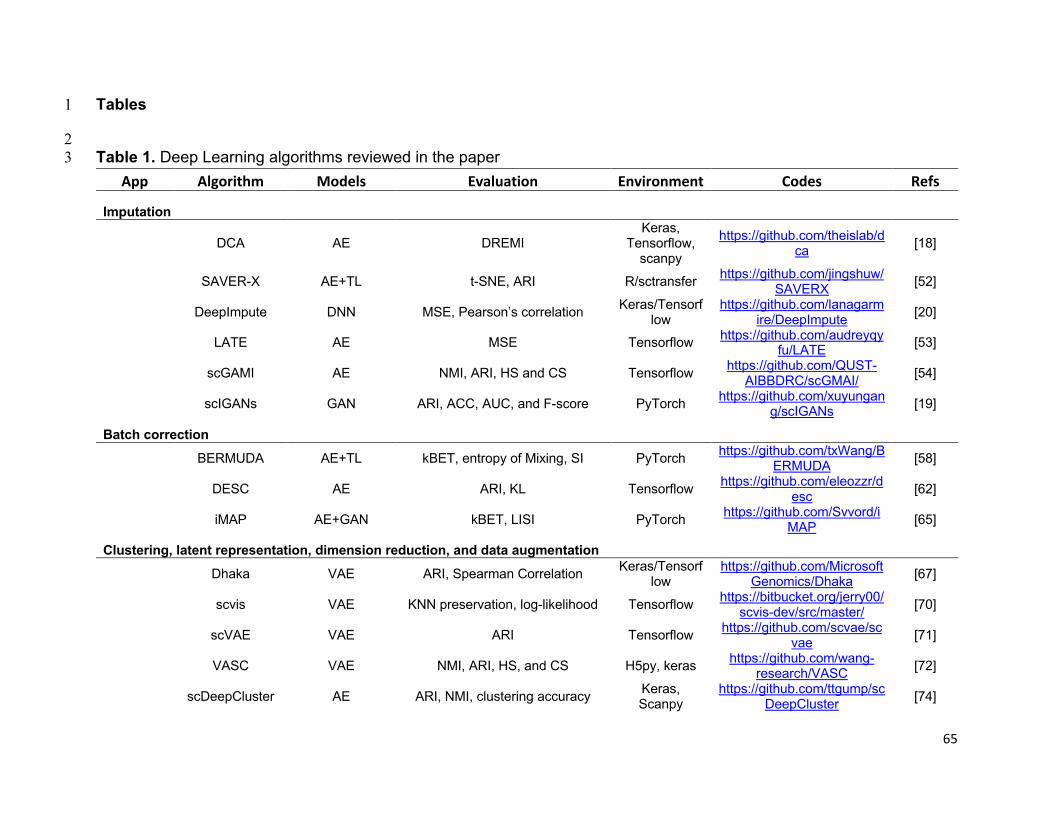
65
Tables 1
2 Table 1. Deep Learning algorithms reviewed in the paper 3
App Algorithm Models Evaluation Environment Codes Refs
Imputation
DCA AE DREMI Keras,
Tensorflow, scanpy
https://github.com/theislab/dca [18]
SAVER-X AE+TL t-SNE, ARI R/sctransfer https://github.com/jingshuw/SAVERX [52]
DeepImpute DNN MSE, Pearson’s correlation Keras/Tensorflow
https://github.com/lanagarmire/DeepImpute [20]
LATE AE MSE Tensorflow https://github.com/audreyqyfu/LATE [53]
scGAMI AE NMI, ARI, HS and CS Tensorflow https://github.com/QUST-AIBBDRC/scGMAI/ [54]
scIGANs GAN ARI, ACC, AUC, and F-score PyTorch https://github.com/xuyungang/scIGANs [19]
Batch correction BERMUDA AE+TL kBET, entropy of Mixing, SI PyTorch https://github.com/txWang/B
ERMUDA [58]
DESC AE ARI, KL Tensorflow https://github.com/eleozzr/desc [62]
iMAP AE+GAN kBET, LISI PyTorch https://github.com/Svvord/iMAP [65]
Clustering, latent representation, dimension reduction, and data augmentation
Dhaka VAE ARI, Spearman Correlation Keras/Tensorflow
https://github.com/MicrosoftGenomics/Dhaka [67]
scvis VAE KNN preservation, log-likelihood Tensorflow https://bitbucket.org/jerry00/scvis-dev/src/master/ [70]
scVAE VAE ARI Tensorflow https://github.com/scvae/scvae [71]
VASC VAE NMI, ARI, HS, and CS H5py, keras https://github.com/wang-research/VASC [72]
scDeepCluster AE ARI, NMI, clustering accuracy Keras, Scanpy
https://github.com/ttgump/scDeepCluster [74]

66
cscGAN GAN t-SNE, marker genes, MMD, AUC Scipy, Tensorflow
https://github.com/imsb-uke/scGAN [77]
Multi-functional models (IM: imputation, BC: batch correction, CL: clustering)
scVI VAE IM: L1 distance; CL: ARI, NMI, SI;
BC: Entropy of Mixing PyTorch, Anndata
https://github.com/YosefLab/scvi-tools [17]
LDVAE VAE Reconstruction errors Part of scVI https://github.com/YosefLab/scvi-tools [81]
SAUCIE AE IM: R2 statistics; CL: SI;
BC: modified kBET; Visualization: Precision/Recall
Tensorflow https://github.com/KrishnaswamyLab/SAUCIE/ [15]
scScope AE IM:Reconstruction errors;
BC: Entropy of mixing; CL: ARI Tensorflow, Scikit-learn
https://github.com/AltschulerWu-Lab/scScope [87]
Cell type Identification DigitalDLSorter DNN Pearson correlation R/Python/Ke
ras https://github.com/cartof/digit
alDLSorter [88]
scCapsNet CapsNet Cell-type Prediction accuracy Keras, Tensorflow
https://github.com/wanglf19/scCaps [95]
netAE VAE Cell-type Prediction accuracy, t-
SNE for visualization pyTorch https://github.com/LeoZDong/netAE [99]
scDGN DANN Prediciton accuracy pyTorch https://github.com/SongweiGe/scDGN [102]
Function analysis CNNC CNN AUROC, AUPRC, and accuracy Keras,
Tensorflow https://github.com/xiaoyeye/
CNNC [105]
scGen VAE Correlation, visualization Tensorflow https://github.com/theislab/scgen [114]
DL Model keywords: AE: autoencoder, AE+TL: autoencoder with transfer learning, AE: variational autoencoder, GAN: Generative adversarial 1 network, CNN: convolutional neural network, DNN: deep neural network, DANN: domain adversarial neural network, CapsNet: capsule neural 2 network 3 4
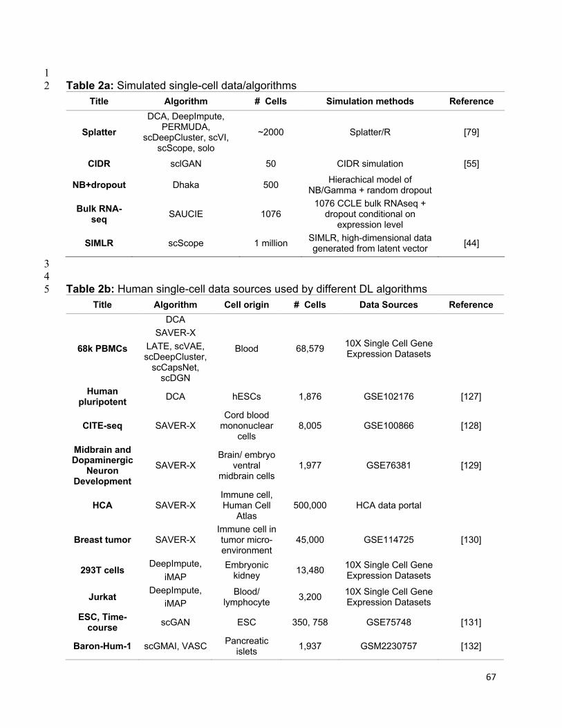
67
1 Table 2a: Simulated single-cell data/algorithms 2
Title Algorithm # Cells Simulation methods Reference
Splatter DCA, DeepImpute,
PERMUDA, scDeepCluster, scVI,
scScope, solo
~2000 Splatter/R [79]
CIDR sclGAN 50 CIDR simulation [55]
NB+dropout Dhaka 500 Hierachical model of NB/Gamma + random dropout
Bulk RNA-seq SAUCIE 1076
1076 CCLE bulk RNAseq + dropout conditional on
expression level
SIMLR scScope 1 million SIMLR, high-dimensional data generated from latent vector [44]
3 4 Table 2b: Human single-cell data sources used by different DL algorithms 5
Title Algorithm Cell origin # Cells Data Sources Reference
68k PBMCs
DCA SAVER-X
LATE, scVAE, scDeepCluster,
scCapsNet, scDGN
Blood 68,579 10X Single Cell Gene Expression Datasets
Human pluripotent DCA hESCs 1,876 GSE102176 [127]
CITE-seq SAVER-X Cord blood
mononuclear cells
8,005 GSE100866 [128]
Midbrain and Dopaminergic
Neuron Development
SAVER-X Brain/ embryo
ventral midbrain cells
1,977 GSE76381 [129]
HCA SAVER-X Immune cell, Human Cell
Atlas 500,000 HCA data portal
Breast tumor SAVER-X Immune cell in tumor micro-environment
45,000 GSE114725 [130]
293T cells DeepImpute, iMAP
Embryonic kidney 13,480 10X Single Cell Gene
Expression Datasets
Jurkat DeepImpute, iMAP
Blood/ lymphocyte 3,200 10X Single Cell Gene
Expression Datasets
ESC, Time-course scGAN ESC 350, 758 GSE75748 [131]
Baron-Hum-1 scGMAI, VASC Pancreatic islets 1,937 GSM2230757 [132]
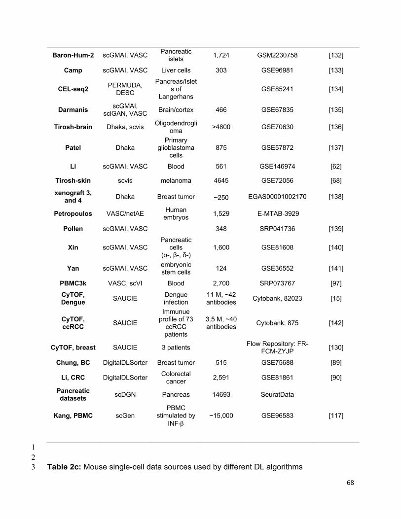
68
Baron-Hum-2 scGMAI, VASC Pancreatic islets 1,724 GSM2230758 [132]
Camp scGMAI, VASC Liver cells 303 GSE96981 [133]
CEL-seq2 PERMUDA, DESC
Pancreas/Islets of
Langerhans GSE85241 [134]
Darmanis scGMAI, sclGAN, VASC Brain/cortex 466 GSE67835 [135]
Tirosh-brain Dhaka, scvis Oligodendroglioma >4800 GSE70630 [136]
Patel Dhaka Primary
glioblastoma cells
875 GSE57872 [137]
Li scGMAI, VASC Blood 561 GSE146974 [62]
Tirosh-skin scvis melanoma 4645 GSE72056 [68]
xenograft 3, and 4 Dhaka Breast tumor ~250 EGAS00001002170 [138]
Petropoulos VASC/netAE Human embryos 1,529 E-MTAB-3929
Pollen scGMAI, VASC 348 SRP041736 [139]
Xin scGMAI, VASC Pancreatic
cells (α-, β-, δ-)
1,600 GSE81608 [140]
Yan scGMAI, VASC embryonic stem cells 124 GSE36552 [141]
PBMC3k VASC, scVI Blood 2,700 SRP073767 [97]
CyTOF, Dengue SAUCIE Dengue
infection 11 M, ~42 antibodies Cytobank, 82023 [15]
CyTOF, ccRCC SAUCIE
Immunue profile of 73
ccRCC patients
3.5 M, ~40 antibodies Cytobank: 875 [142]
CyTOF, breast SAUCIE 3 patients Flow Repository: FR-FCM-ZYJP [130]
Chung, BC DigitalDLSorter Breast tumor 515 GSE75688 [89]
Li, CRC DigitalDLSorter Colorectal cancer 2,591 GSE81861 [90]
Pancreatic datasets scDGN Pancreas 14693 SeuratData
Kang, PBMC scGen PBMC
stimulated by INF-b
~15,000 GSE96583 [117]
1 2 Table 2c: Mouse single-cell data sources used by different DL algorithms 3
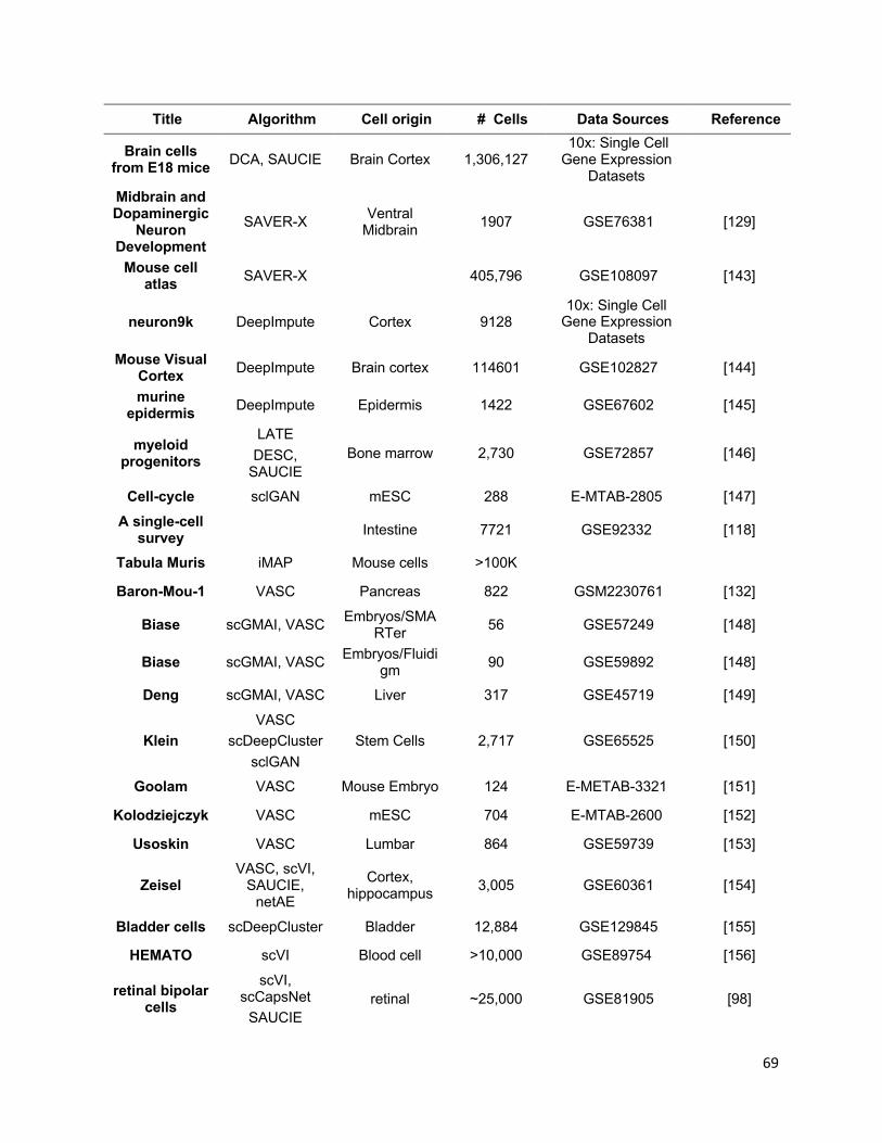
69
Title Algorithm Cell origin # Cells Data Sources Reference
Brain cells from E18 mice DCA, SAUCIE Brain Cortex 1,306,127
10x: Single Cell Gene Expression
Datasets
Midbrain and Dopaminergic
Neuron Development
SAVER-X Ventral Midbrain 1907 GSE76381 [129]
Mouse cell atlas SAVER-X 405,796 GSE108097 [143]
neuron9k DeepImpute Cortex 9128 10x: Single Cell
Gene Expression Datasets
Mouse Visual Cortex DeepImpute Brain cortex 114601 GSE102827 [144]
murine epidermis DeepImpute Epidermis 1422 GSE67602 [145]
myeloid progenitors
LATE DESC,
SAUCIE Bone marrow 2,730 GSE72857 [146]
Cell-cycle sclGAN mESC 288 E-MTAB-2805 [147]
A single-cell survey Intestine 7721 GSE92332 [118]
Tabula Muris iMAP Mouse cells >100K
Baron-Mou-1 VASC Pancreas 822 GSM2230761 [132]
Biase scGMAI, VASC Embryos/SMARTer 56 GSE57249 [148]
Biase scGMAI, VASC Embryos/Fluidigm 90 GSE59892 [148]
Deng scGMAI, VASC Liver 317 GSE45719 [149]
Klein VASC
scDeepCluster sclGAN
Stem Cells 2,717 GSE65525 [150]
Goolam VASC Mouse Embryo 124 E-METAB-3321 [151]
Kolodziejczyk VASC mESC 704 E-MTAB-2600 [152]
Usoskin VASC Lumbar 864 GSE59739 [153]
Zeisel VASC, scVI,
SAUCIE, netAE
Cortex, hippocampus 3,005 GSE60361 [154]
Bladder cells scDeepCluster Bladder 12,884 GSE129845 [155]
HEMATO scVI Blood cell >10,000 GSE89754 [156]
retinal bipolar cells
scVI, scCapsNet
SAUCIE retinal ~25,000 GSE81905 [98]
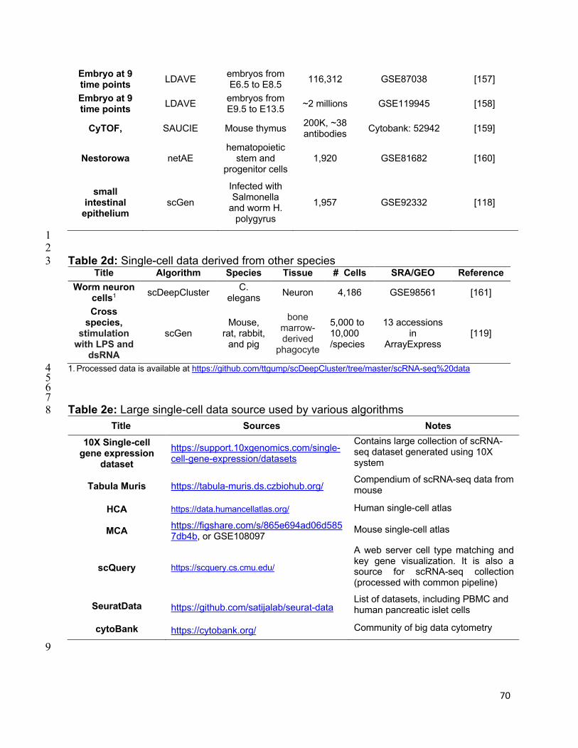
70
Embryo at 9 time points LDAVE embryos from
E6.5 to E8.5 116,312 GSE87038 [157]
Embryo at 9 time points LDAVE embryos from
E9.5 to E13.5 ~2 millions GSE119945 [158]
CyTOF, SAUCIE Mouse thymus 200K, ~38 antibodies Cytobank: 52942 [159]
Nestorowa netAE hematopoietic
stem and progenitor cells
1,920 GSE81682 [160]
small intestinal
epithelium scGen
Infected with Salmonella
and worm H. polygyrus
1,957 GSE92332 [118]
1 2 Table 2d: Single-cell data derived from other species 3
Title Algorithm Species Tissue # Cells SRA/GEO Reference Worm neuron
cells1 scDeepCluster C. elegans Neuron 4,186 GSE98561 [161]
Cross species,
stimulation with LPS and
dsRNA
scGen Mouse,
rat, rabbit, and pig
bone marrow-derived
phagocyte
5,000 to 10,000 /species
13 accessions in
ArrayExpress [119]
1. Processed data is available at https://github.com/ttgump/scDeepCluster/tree/master/scRNA-seq%20data 4 5 6 7 Table 2e: Large single-cell data source used by various algorithms 8
Title Sources Notes
10X Single-cell gene expression
dataset https://support.10xgenomics.com/single-cell-gene-expression/datasets
Contains large collection of scRNA-seq dataset generated using 10X system
Tabula Muris https://tabula-muris.ds.czbiohub.org/ Compendium of scRNA-seq data from mouse
HCA https://data.humancellatlas.org/ Human single-cell atlas
MCA https://figshare.com/s/865e694ad06d5857db4b, or GSE108097
Mouse single-cell atlas
scQuery https://scquery.cs.cmu.edu/
A web server cell type matching and key gene visualization. It is also a source for scRNA-seq collection (processed with common pipeline)
SeuratData https://github.com/satijalab/seurat-data List of datasets, including PBMC and human pancreatic islet cells
cytoBank https://cytobank.org/ Community of big data cytometry
9

71
Table 3. Evaluation metrics used in surveyed DL algorithms Evaluation Method Equations Explanation
Pseudobulk RNA-seq
Average of normalized (log2-transformed) scRNA-seq counts across cells is calculated and then correlation coefficient between the pseudobulk and the actual bulk RNA-seq profile of the same cell type is evaluated.
Mean squared error (MSE) !"# =
1&'()! − )+!)"#
!$%
MSE assesses the quality of a predictor, or an estimator, from a collection of observed data x, with )+ being the predicted values.
Pearson correlation -&,( =/01(2, 4)5&5(
where cov() is the covariance, sX and sY are the standard deviation of X and Y, respectively.
Spearman correlation -) = -*!,*" =/01(6&, 6()5*!5*"
The Spearman correlation coefficient is defined as the Pearson correlation coefficient between the rank variables, where rX is the rank of X.
Entropy of accuracy, Hacc [21] 7+,, = −
1!''8!9)-: log >8!9)-:?
.#
-$%
/
!$%
Measures the diversity of the ground-truth labels within each predicted cluster group. pi(xj) (or qi(xj)) are the proportions of cells in the jth ground-truth cluster (or predicted cluster) relative to the total number of cells in the ith predicted cluster (or ground-truth clusters), respectively.
Entropy of purity, Hpur [21] 701* = −1@''A!9)-: log >A!9)-:?
/#
-$%
.
!$%
Measures the diversity of the predicted cluster labels within each ground-truth group
Entropy of mixing [32] # ='8! log(8!)2
!$%
This metric evaluates the mixing of cells from different batches in the neighborhood of each cell. C is the number of batches, and 8! is the proportion of cells from batch B among N nearest cells.
Mutual Information (MI) [162] !C(D, E) =''F34(B, G) log H
F34(B, G)F3(B)F4(G)
I
|4|
-$%
|3|
!$%
where F3(B) =|3#|. and F4(G) =
64$6. . Also, define the joint
distribution probability is F34(B, G) =63#∩4$6
. . The MI is a measure of mutual dependency between two cluster assignments U and V.
Normalized Mutual Information (NMI) [163] @!C(D, E) =
2 ×!C(D, E)[7(D) + 7(E)]
where 7(D) = ∑F3(B) log9F3(B): , 7(E) = ∑F4(B) log9F4(B):. The NMI is a normalization of the MI score between 0 and 1.
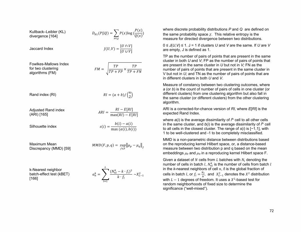
72
Kullback–Leibler (KL) divergence [164]
P89(F||R) ='F())log(F())R())
):∈<
where discrete probability distributions P and Q are defined on the same probability space c. This relative entropy is the measure for directed divergence between two distributions.
Jaccard Index S(D, E) =⌊D ∩ E⌋⌊D ∪ E⌋
0 ≤ J(U,V) ≤ 1. J = 1 if clusters U and V are the same. If U are V are empty, J is defined as 1.
Fowlkes-Mallows Index for two clustering algorithms (FM)
X! =YZF
ZF + XF×
ZFZF + X@
TP as the number of pairs of points that are present in the same cluster in both U and V; FP as the number of pairs of points that are present in the same cluster in U but not in V; FN as the number of pairs of points that are present in the same cluster in V but not in U; and TN as the number of pairs of points that are in different clusters in both U and V.
Rand index (RI) [C = (\ + ])/ >&2?
Measure of constancy between two clustering outcomes, where a (or b) is the count of number of pairs of cells in one cluster (or different clusters) from one clustering algorithm but also fall in the same cluster (or different clusters) from the other clustering algorithm.
Adjusted Rand index (ARI) [165] _[C =
[C − #[[C]max([C) − #[[C]
ARI is a corrected-for-chance version of RI, where E[RI] is the expected Rand Index.
Silhouette index c(B) =](B) − \(B)
max(\(B), ](B))
where a(i) is the average dissimilarity of ith cell to all other cells in the same cluster, and b(i) is the average dissimilarity of ith cell to all cells in the closest cluster. The range of s(i) is [−1,1], with 1 to be well-clustered and -1 to be completely misclassified.
Maximum Mean Discrepancy (MMD) [59]
!!P(X, 8, A) = cd8=∈>
ef0 − f?e= MMD is a non-parametric distance between distributions based on the reproducing kernel Hilbert space, or, a distance-based measure between two distribution p and q based on the mean embeddings µp and µq in a reproducing kernel Hilbert space F.
k-Nearest neighbor batch-effect test (kBET) [166]
\#@ =g(@#A
@ − h ∙ jA)"
h ∙ jA
9
A$%
~29B%"
Given a dataset of @ cells from l batches with @A denoting the number of cells in batch m, @#A@ is the number of cells from batch m in the k-nearest neighbors of cell &, fl is the global fraction of cells in batch m, or jA =
.%
. , and 29B%" denotes the 2" distribution with l − 1 degrees of freedom. It uses a 2"-based test for random neighborhoods of fixed size to determine the significance (“well-mixed”).
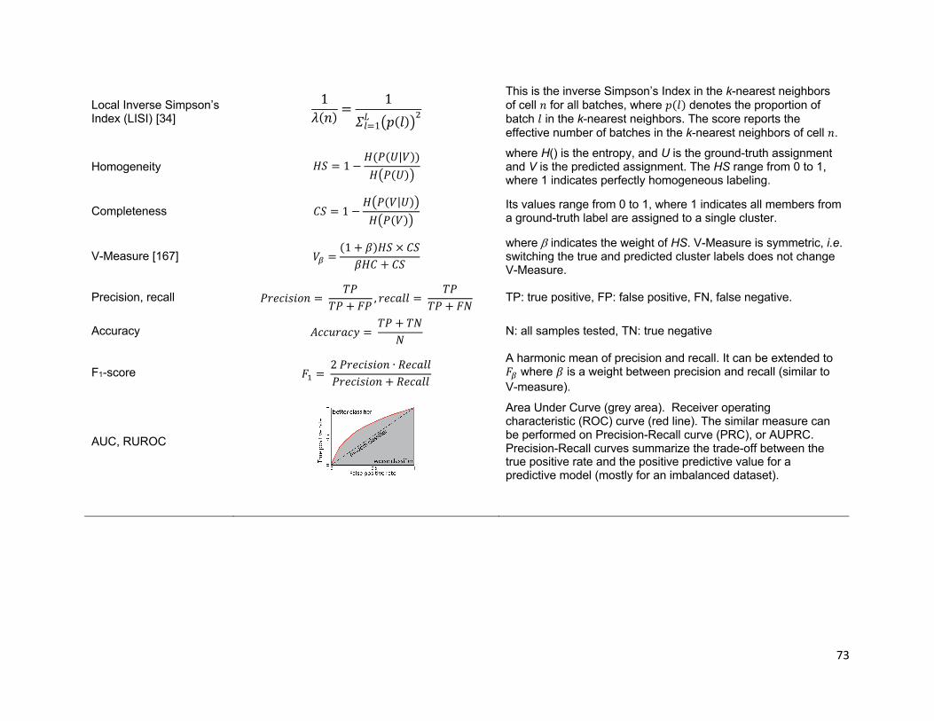
73
Local Inverse Simpson’s Index (LISI) [34]
1"(#) =
1%!=1$ #&(')$!
This is the inverse Simpson’s Index in the k-nearest neighbors of cell & for all batches, where 8(m) denotes the proportion of batch m in the k-nearest neighbors. The score reports the effective number of batches in the k-nearest neighbors of cell &.
Homogeneity 7" = 1 −7(F(D|E))
79F(D):
where H() is the entropy, and U is the ground-truth assignment and V is the predicted assignment. The HS range from 0 to 1, where 1 indicates perfectly homogeneous labeling.
Completeness n" = 1 −79F(E|D):
79F(E): Its values range from 0 to 1, where 1 indicates all members from
a ground-truth label are assigned to a single cluster.
V-Measure [167] EC =(1 + o)7" × n"o7n + n"
where b indicates the weight of HS. V-Measure is symmetric, i.e. switching the true and predicted cluster labels does not change V-Measure.
Precision, recall F6p/BcB0& = ZF
ZF + XF, 6p/\mm =
ZFZF + X@
TP: true positive, FP: false positive, FN, false negative.
Accuracy _//d6\/q = ZF + Z@
@ N: all samples tested, TN: true negative
F1-score X% =2F6p/BcB0& ∙ [p/\mmF6p/BcB0& + [p/\mm
A harmonic mean of precision and recall. It can be extended to XC where o is a weight between precision and recall (similar to V-measure).
AUC, RUROC
Area Under Curve (grey area). Receiver operating characteristic (ROC) curve (red line). The similar measure can be performed on Precision-Recall curve (PRC), or AUPRC. Precision-Recall curves summarize the trade-off between the true positive rate and the positive predictive value for a predictive model (mostly for an imbalanced dataset).

74


![Deep Learning for Multiple-Image Super-ResolutionB. Deep learning for single-image super-resolution Inspired by earlier approaches based on sparse coding [3], Dong et al. proposed](https://img.pdfslide.tips/doc/110x75/5f9dc05f67486a66304e7690/deep-learning-for-multiple-image-super-resolution-b-deep-learning-for-single-image.jpg)