Embed Size (px)
Citation preview

Prof. Dr. Barbara Wohlmuth
Lehrstuhl fur Numerische Mathematik
Definition A-stabil
Wir betrachen das Modellproblem:
y′(t) = λy(t)
y(0) = 1fur λ ∈ C, mit Re(λ) < 0
• Ein Verfahren heißt absolut stabil, falls limi→∞ |yi| = 0.
• Sei yi+1 = R(z)yi, z = hλ, dann die R(z) heißt Stabilitatsfunktion.
• Das Stabilitatsgebiet A ist definiert als
A :=
hλ ∈ C : limi→∞
|yi| = 0,
=
z ∈ C : |R(z)| < 1
,
d.h. die approximative und analytische Losungen haben gleiche asymptotischeEigenschaften.
• Ein Verfahren heißt A-stabil, falls C− ⊂ A
– Typeset by FoilTEX – 1
Prof. Dr. Barbara Wohlmuth
Lehrstuhl fur Numerische Mathematik
Stabilitatsgebiete A
-3 -2 -1 0 1 2 3
x
-3
-2
-1
0
1
2
3
yExplicit Euler
-3 -2 -1 0 1 2 3
x
-3
-2
-1
0
1
2
3
y
Heun
-3 -2 -1 0 1 2 3
x
-3
-2
-1
0
1
2
3
y
Implicit Euler
-3 -2 -1 0 1 2 3
x
-3
-2
-1
0
1
2
3
y
Crank-Nicolson
– Typeset by FoilTEX – 2

Prof. Dr. Barbara Wohlmuth
Lehrstuhl fur Numerische Mathematik
Stabilitatsgebiete A
-3 -2 -1 0 1 2 3
x
-3
-2
-1
0
1
2
3
yRK3
-3 -2 -1 0 1 2 3
x
-3
-2
-1
0
1
2
3
y
RK4
-15 -10 -5 0 5 10
x
-10
-8
-6
-4
-2
0
2
4
6
8
10
y
Hammer & Hollingsworth 4
-15 -10 -5 0 5 10
x
-10
-8
-6
-4
-2
0
2
4
6
8
10
y
Radau 2
– Typeset by FoilTEX – 3

Prof. Dr. Barbara Wohlmuth
Lehrstuhl fur Numerische Mathematik
RLC-Glied
Aufgabe: Beschreibe den zeitlichen Verlauf der Spannung u(t)am Kondensator C, nachdem der Schalter geschlossen wurde.
Nach dem Ohm’schen Gesetz und der Kirchhoff’schen Maschenregel gilt furdie Spannung u(t):
u = U −Ri1 − Li′1
i1 = i2 + i3, wobei i2 =u
Rund i3 = Cu′,
wo i1(t), i2(t) und i3(t) die Strome, wie im Bild oben angedeutet, sind.
– Typeset by FoilTEX – 4

Prof. Dr. Barbara Wohlmuth
Lehrstuhl fur Numerische Mathematik
RLC-Glied: die approximative Losung
Das Gleichungsystem lautet:(u′1
u′2
)
=
(0 1
− 2LC
− 1LC
(RC + RC)
)
︸ ︷︷ ︸=A
(u1
u2
)
+
(0ULC
)
0 0.02 0.04 0.06 0.08 0.10
1
2
3
4
5potential drop u(t): Explicit Euler
h=0.01h=0.005h=0.001h=0.0005
0 0.02 0.04 0.06 0.08 0.10
0.5
1
1.5
2
2.5
3potential drop u(t): Implizit Euler
h=0.01h=0.005h=0.001h=0.0005
Parametherwahl: L = 0.1, C = 10−3, R = 10, U = 5, u(0) = 0, u′(0) = 0.
Die Matrix A besitzt dann die Eigenwerte λ1,2 = 100 ± 100i, damit folgt diebedingt-Stabilitat fur das expliziten Euler Verfahren fur h < 2
max(|λi|)= 0.01.
– Typeset by FoilTEX – 5

Prof. Dr. Barbara Wohlmuth
Lehrstuhl fur Numerische Mathematik
Definition L-stabil
Obwohl das Verfahren A-stabil ist, konnen lokale Oszilationen in der approximativenLosung auftreten.
Ein RKV heißt L-stabil, falls es A-stabil ist und zusatzlich gilt:
lim|z|→∞
R(z) = 0.
Bemerkung:
Explizite RKV konnen dann auch nicht L-stabil sein.Fur implizite RKV mit R(z) = P (z)
Q(z) muss gelten: deg(P ) < deg(Q).
– Typeset by FoilTEX – 6
Prof. Dr. Barbara Wohlmuth
Lehrstuhl fur Numerische Mathematik
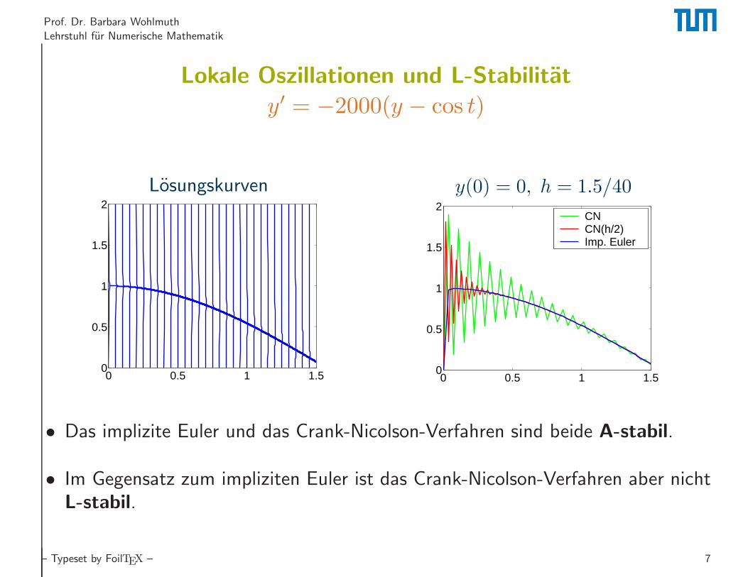
Lokale Oszillationen und L-Stabilitat
y′ = −2000(y − cos t)
Losungskurven
0 0.5 1 1.50
0.5
1
1.5
2y(0) = 0, h = 1.5/40
0 0.5 1 1.50
0.5
1
1.5
2CNCN(h/2)Imp. Euler
• Das implizite Euler und das Crank-Nicolson-Verfahren sind beide A-stabil.
• Im Gegensatz zum impliziten Euler ist das Crank-Nicolson-Verfahren aber nichtL-stabil.
– Typeset by FoilTEX – 7

Prof. Dr. Barbara Wohlmuth
Lehrstuhl fur Numerische Mathematik
Zwischen Crank–Nicolson und implizitem Euler
yi+1 = yi + h ((1− α)fi + αfi+1)
0 0.5 1 1.50
0.5
1
1.5
2alpha = 0.5
0 0.5 1 1.50
0.5
1
1.5
2alpha = 0.6
0 0.5 1 1.50
0.5
1
1.5
2alpha = 0.7
0 0.5 1 1.50
0.5
1
1.5
2alpha = 0.8
0 0.5 1 1.50
0.5
1
1.5
2alpha = 0.9
0 0.5 1 1.50
0.5
1
1.5
2alpha = 1.0
– Typeset by FoilTEX – 8

Prof. Dr. Barbara Wohlmuth
Lehrstuhl fur Numerische Mathematik
Definition B-stabil
• Sei f : Ω → Rd, Ω ⊂ R
d, f heißt streng dissipativ, falls
〈f(y)− f(y), y − y〉 < 0, ∀y, y ∈ Ω.
• Wendet man ein RKV auf ein AWP mit dissipativer rechter Seite an, so heißtdieses RKV B-stabil, falls fur h > 0 folgt:
‖y1 − y1‖ 6 ‖y0 − y0‖ ,
wobei y1 := y0 + hΦ(t0, h, y0, y1) und y1 := y0 + hΦ(t0, h, y0, y1) und Φ dieVerfahrensfunktion des RKV ist.
Bemerkung: B-stabile Verfahren sind auch A-stabil.Bei dissipativen Systemen nimmt also der Einfluß einer kleinen Storung in den ABnicht mit der Zeit zu.
– Typeset by FoilTEX – 9

Prof. Dr. Barbara Wohlmuth
Lehrstuhl fur Numerische Mathematik
Beispiel: B-Stabilitat
Sei y′ = f(y), wobei f (streng) dissipativ ist:
f(y) =
y2, falls y 6 0
−y2, falls y > 0
y(0) = 0, y(0) = −2 ⇒ |y0 − y0| = 2.
|yi−
yi|
0 10 20 300
0.5
1
1.5
2
time
Implizites−Euler−Verfahren
|yi−
yi|
0 10 20 300
1
2
3
4
time
Crank−Nicolson−Verfahren
Das implizite Euler erhalt im Gegensatz zum Crank-Nicolson-Verfahrendie Dissipativitat der approximativen Losung.
– Typeset by FoilTEX – 10

Prof. Dr. Barbara Wohlmuth
Lehrstuhl fur Numerische Mathematik
Steifes Problem
y′ = −1000y + 3000− 2000e−t, y(0) = 0
Exakte Losung: y = −0.998e−1000t︸ ︷︷ ︸
schnell abklingender Term
+ 3− 2.002e−t︸ ︷︷ ︸
langsamer abklingender Term
0 5 10-1
-0.8
-0.6
-0.4
-0.2
0fast term y
1 = -0.998 e-1000 t
0 5 10-2.5
-2
-1.5
-1
-0.5
0slow term y
2 = - 2.002 e-t
0 5 100
0.5
1
1.5
2
2.5
3
exact solution yex
= 3 + y1 + y
2
– Typeset by FoilTEX – 11

Prof. Dr. Barbara Wohlmuth
Lehrstuhl fur Numerische Mathematik
Steifes Problem
y′ = −1000y + 3000− 2000e−t, y(0) = 0
0 5 1010-100
10 -50
10 0
10 50
10 100explicit Euler, h = 0.5
0 5 100
1
2
3
4implicit Euler, h = 0.5
0 5 100
1
2
3
4Crank-Nicolson, h = 0.5
0 5 1010-200
10-100
10 0
10 100
10 200explicit Euler, h = 0.1
0 5 100
1
2
3
4implicit Euler, h = 0.1
0 5 100
1
2
3
4Crank-Nicolson, h = 0.1
– Typeset by FoilTEX – 12
Prof. Dr. Barbara Wohlmuth
Lehrstuhl fur Numerische Mathematik
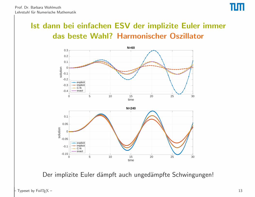
Ist dann bei einfachen ESV der implizite Euler immer
das beste Wahl? Harmonischer Oszillator
0 5 10 15 20 25 30time
-0.4
-0.3
-0.2
-0.1
0
0.1
0.2
0.3
solu
tion
N=60
explicitimplicitC-Nexact
0 5 10 15 20 25 30time
-0.15
-0.1
-0.05
0
0.05
0.1
solu
tion
N=240
explicitimplicitC-Nexact
Der implizite Euler dampft auch ungedampfte Schwingungen!
– Typeset by FoilTEX – 13