Embed Size (px)
Citation preview
7/21/2019 Dept Fall2013
http://slidepdf.com/reader/full/dept-fall2013 1/57
Viscoelastic Fluids Mathematical Models of Viscoelastic Flows Numerical Methods of Viscoelastic Flow Simulations Preliminary Results
Mathematical Models and Computational Methodsfor Viscoelastic Fluids
Olabanji Y. ShonibareAdvisors: Prof. Kathleen Feigl & Prof. Franz Tanner
February 16, 2015
7/21/2019 Dept Fall2013
http://slidepdf.com/reader/full/dept-fall2013 2/57
Viscoelastic Fluids Mathematical Models of Viscoelastic Flows Numerical Methods of Viscoelastic Flow Simulations Preliminary Results
Contents
1 Viscoelastic Fluids
Introduction
Flow Behaviour of Viscoelastic Fluids Vs Newtonian Fluids
2 Mathematical Models of Viscoelastic Flows
Conservation Equation of Continuum MechanicsRheology and Constitutive Equations
Memory Fluids
3 Numerical Methods of Viscoelastic Flow Simulations
Governing EquationsDiscretization of the Transport Equation
Iterative Solution Algorithm
4 Preliminary Results
7/21/2019 Dept Fall2013
http://slidepdf.com/reader/full/dept-fall2013 3/57
Viscoelastic Fluids Mathematical Models of Viscoelastic Flows Numerical Methods of Viscoelastic Flow Simulations Preliminary Results
Introduction
Viscoelastic Fluids
They are fluids that possess both viscous and “elastic” properties. Theyexhibit flow phenomena that cannot be explained by the Newtonian
Viscous law e.g. Weissenberg effect . Hence, they are also referred tonon-Newtonian fluids .
Examples of non-Newtonian fluids are Polymeric fluids used to makeplastic articles, dough used to make bread and pasta, biological fluidssuch as synovial fluids found in joints and blood.
7/21/2019 Dept Fall2013
http://slidepdf.com/reader/full/dept-fall2013 4/57
Viscoelastic Fluids Mathematical Models of Viscoelastic Flows Numerical Methods of Viscoelastic Flow Simulations Preliminary Results
Flow Behaviour of Viscoelastic Fluids Vs Newtonian Fluids
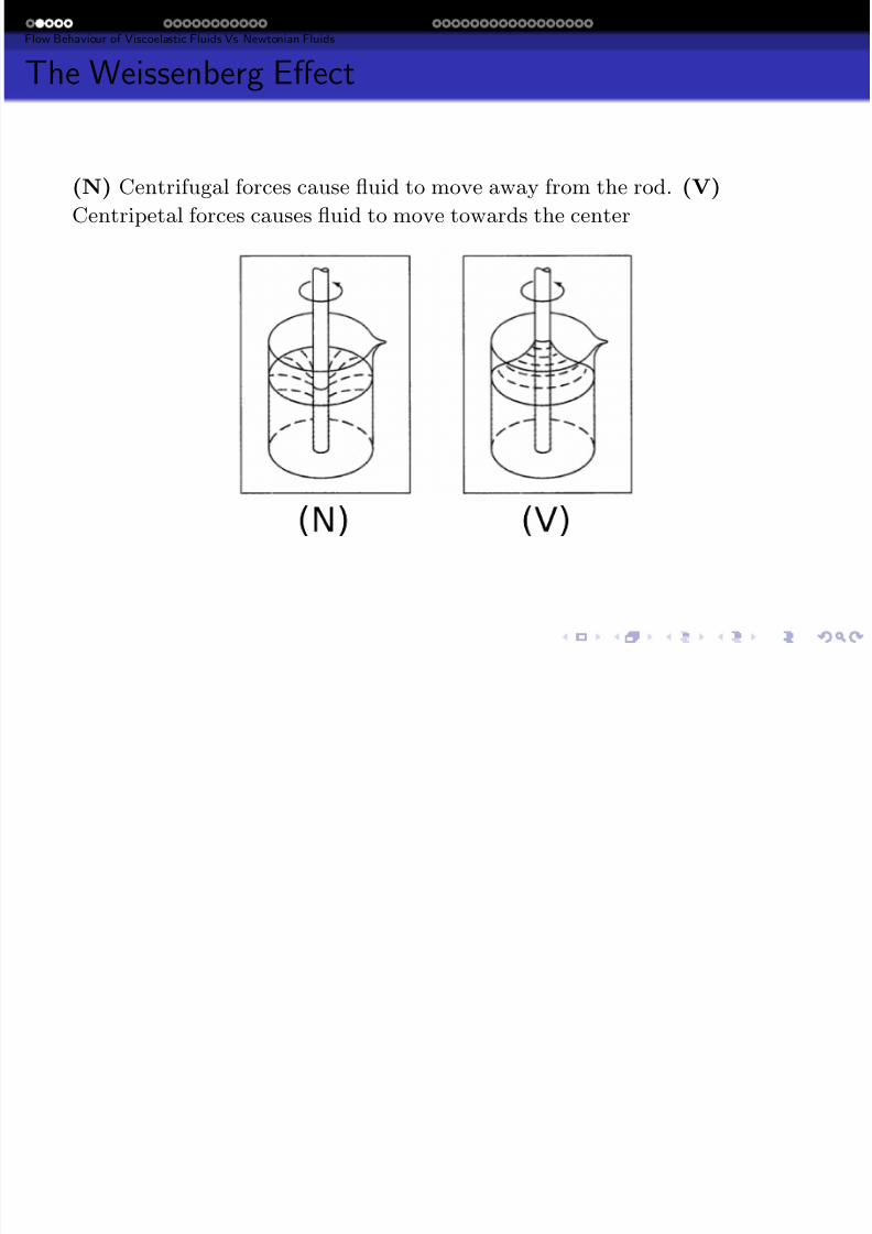
The Weissenberg Effect
(N) Centrifugal forces cause fluid to move away from the rod. (V)
Centripetal forces causes fluid to move towards the center
Vi l i Fl id M h i l M d l f Vi l i Fl N i l M h d f Vi l i Fl Si l i P li i R l
7/21/2019 Dept Fall2013
http://slidepdf.com/reader/full/dept-fall2013 5/57
Viscoelastic Fluids Mathematical Models of Viscoelastic Flows Numerical Methods of Viscoelastic Flow Simulations Preliminary Results
Flow Behaviour of Viscoelastic Fluids Vs Newtonian Fluids
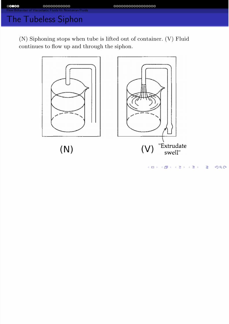
The Tubeless Siphon
(N) Siphoning stops when tube is lifted out of container. (V) Fluidcontinues to flow up and through the siphon.
Viscoelastic Fl ids Mathematical Models of Viscoelastic Flo s N merical Methods of Viscoelastic Flo Sim lations Preliminar Res lts
7/21/2019 Dept Fall2013
http://slidepdf.com/reader/full/dept-fall2013 6/57
Viscoelastic Fluids Mathematical Models of Viscoelastic Flows Numerical Methods of Viscoelastic Flow Simulations Preliminary Results
Flow Behaviour of Viscoelastic Fluids Vs Newtonian Fluids
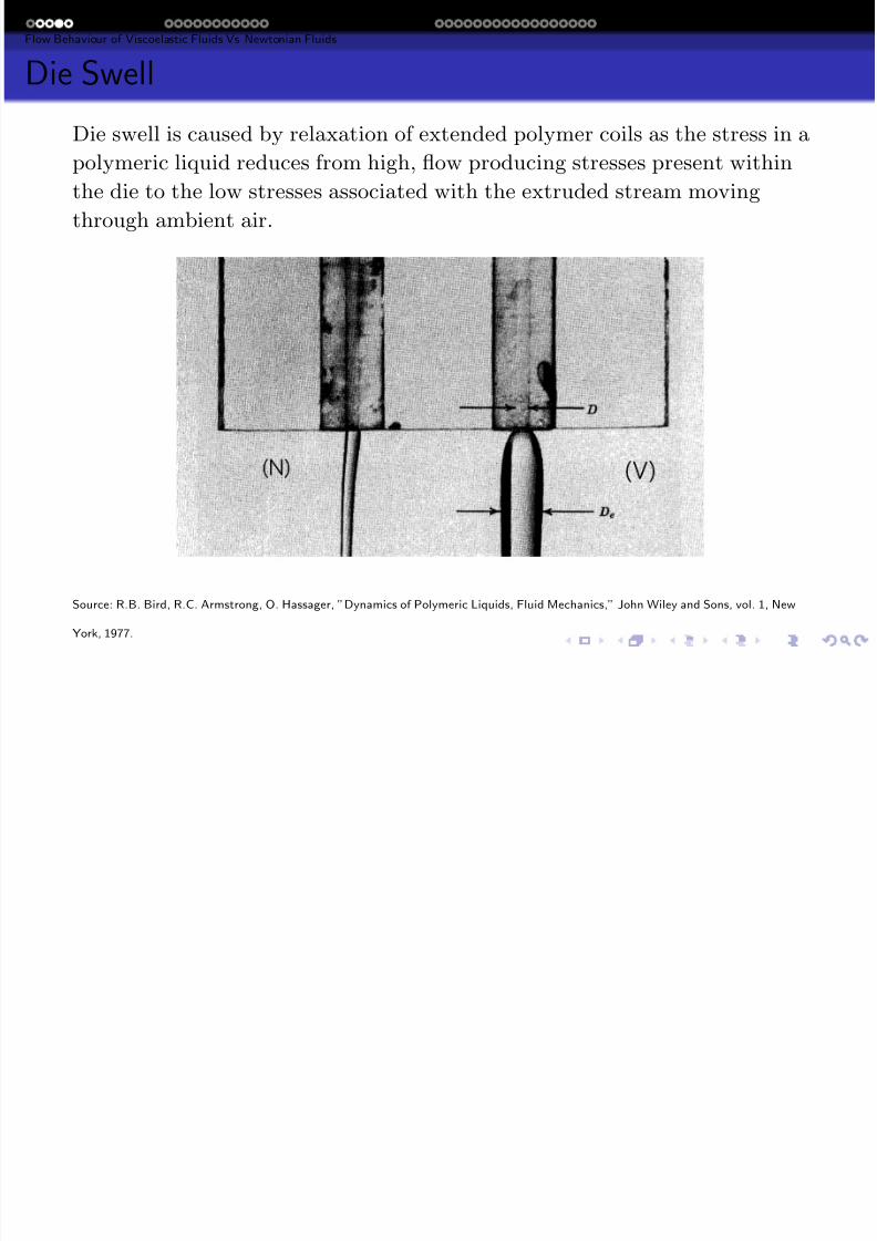
Die Swell
Die swell is caused by relaxation of extended polymer coils as the stress in a
polymeric liquid reduces from high, flow producing stresses present within
the die to the low stresses associated with the extruded stream moving
through ambient air.
Source: R.B. Bird, R.C. Armstrong, O. Hassager, ”Dynamics of Polymeric Liquids, Fluid Mechanics,” John Wiley and Sons, vol. 1, New
York, 1977.
Viscoelastic Fluids Mathematical Models of Viscoelastic Flows Numerical Methods of Viscoelastic Flow Simulations Preliminary Results
7/21/2019 Dept Fall2013
http://slidepdf.com/reader/full/dept-fall2013 7/57
Viscoelastic Fluids Mathematical Models of Viscoelastic Flows Numerical Methods of Viscoelastic Flow Simulations Preliminary Results
Flow Behaviour of Viscoelastic Fluids Vs Newtonian Fluids
Dimensionless Groups
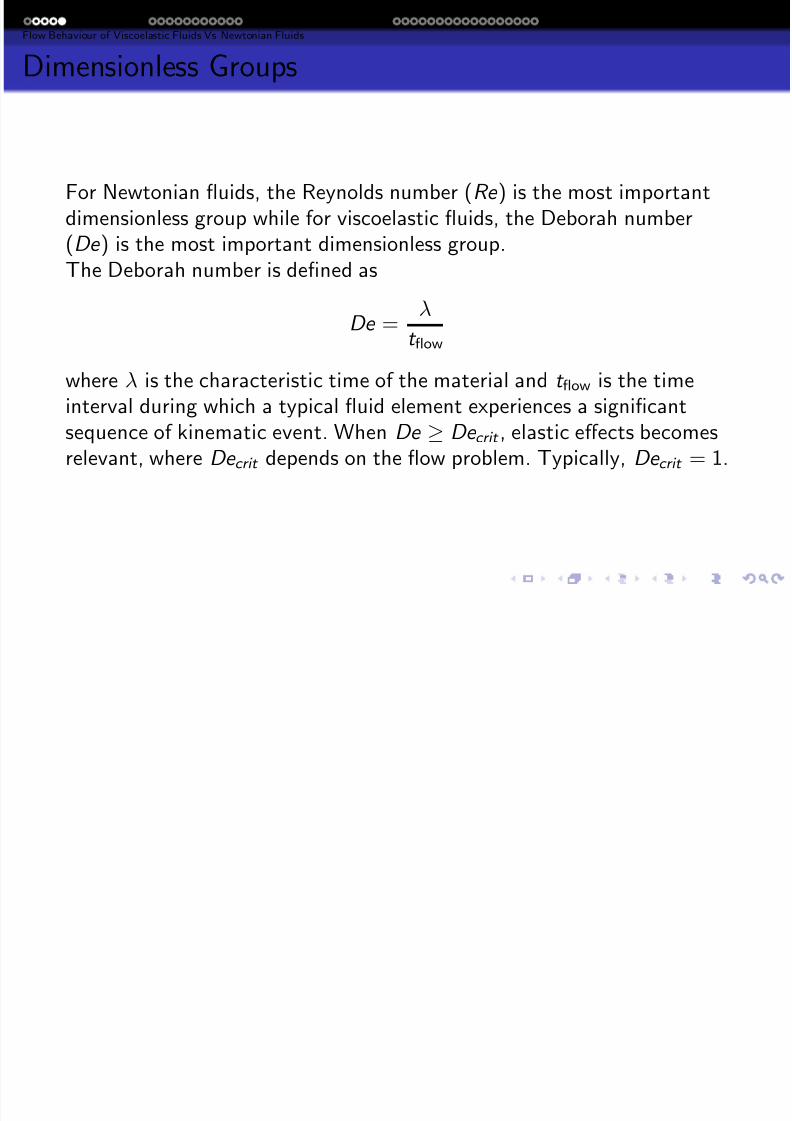
For Newtonian fluids, the Reynolds number (Re ) is the most importantdimensionless group while for viscoelastic fluids, the Deborah number(De ) is the most important dimensionless group.
The Deborah number is defined as
De = λ
t flow
where λ is the characteristic time of the material and t flow is the time
interval during which a typical fluid element experiences a significantsequence of kinematic event. When De ≥ De crit , elastic effects becomesrelevant, where De crit depends on the flow problem. Typically, De crit = 1.
Viscoelastic Fluids Mathematical Models of Viscoelastic Flows Numerical Methods of Viscoelastic Flow Simulations Preliminary Results
7/21/2019 Dept Fall2013
http://slidepdf.com/reader/full/dept-fall2013 8/57
Viscoelastic Fluids Mathematical Models of Viscoelastic Flows Numerical Methods of Viscoelastic Flow Simulations Preliminary Results
Contents
1 Viscoelastic Fluids
Introduction
Flow Behaviour of Viscoelastic Fluids Vs Newtonian Fluids
2 Mathematical Models of Viscoelastic Flows
Conservation Equation of Continuum MechanicsRheology and Constitutive Equations
Memory Fluids
3 Numerical Methods of Viscoelastic Flow Simulations
Governing Equations
Discretization of the Transport Equation
Iterative Solution Algorithm
4 Preliminary Results
Viscoelastic Fluids Mathematical Models of Viscoelastic Flows Numerical Methods of Viscoelastic Flow Simulations Preliminary Results
7/21/2019 Dept Fall2013
http://slidepdf.com/reader/full/dept-fall2013 9/57
Viscoelastic Fluids Mathematical Models of Viscoelastic Flows Numerical Methods of Viscoelastic Flow Simulations Preliminary Results
Conservation Equation of Continuum Mechanics
Conservation Equation
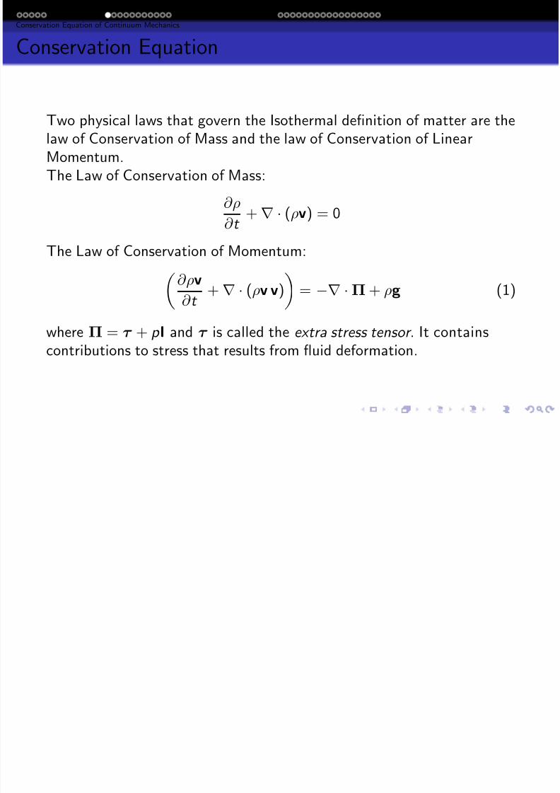
Two physical laws that govern the Isothermal definition of matter are thelaw of Conservation of Mass and the law of Conservation of LinearMomentum.The Law of Conservation of Mass:
∂ρ
∂ t + ∇ · (ρv) = 0
The Law of Conservation of Momentum:
∂ρv
∂ t + ∇ · (ρv v)
= −∇ ·Π + ρg (1)
where Π = τ + p I and τ is called the extra stress tensor . It containscontributions to stress that results from fluid deformation.
Viscoelastic Fluids Mathematical Models of Viscoelastic Flows Numerical Methods of Viscoelastic Flow Simulations Preliminary Results
7/21/2019 Dept Fall2013
http://slidepdf.com/reader/full/dept-fall2013 10/57
y
Rheology and Constitutive Equations
Constitutive Equation
A Constitutive equation is an equation that expresses the molecularstresses generated in the flow in terms of kinetic variables such asvelocities, derivatives of velocities and strain.
Viscoelastic Fluids Mathematical Models of Viscoelastic Flows Numerical Methods of Viscoelastic Flow Simulations Preliminary Results
7/21/2019 Dept Fall2013
http://slidepdf.com/reader/full/dept-fall2013 11/57
y
Rheology and Constitutive Equations
Newtonian Fluids
The Constitutive Equation for an Incompressible Newtonian Fluid is givenby
τ = −µγ̇ (2)
where γ̇ , the rate of strain tensor is given by
γ̇ = ∇v + (∇v)T
Viscoelastic Fluids Mathematical Models of Viscoelastic Flows Numerical Methods of Viscoelastic Flow Simulations Preliminary Results
7/21/2019 Dept Fall2013
http://slidepdf.com/reader/full/dept-fall2013 12/57
Memory Fluids
Memory Fluids
For Generalized Newtonian Constitutive Equation,
τ (t ) = −η(γ̇ )γ̇ (t ).
Since γ̇ (t ) represents only the instantaneous deformation, there can beno effect of the history of the deformation on the stress in these models.
To construct a Constitutive equation with memory, we must includeterms that involve expressions such as γ̇ (t − t o ), the value of γ̇ at a time
t o seconds in the past.
Viscoelastic Fluids Mathematical Models of Viscoelastic Flows Numerical Methods of Viscoelastic Flow Simulations Preliminary Results
7/21/2019 Dept Fall2013
http://slidepdf.com/reader/full/dept-fall2013 13/57
Memory Fluids
Maxwell Model
The Maxwell fluid Constitutive Model (differential form),
τ + λ∂ τ
∂ t = −ηo γ̇
Viscoelastic Fluids Mathematical Models of Viscoelastic Flows Numerical Methods of Viscoelastic Flow Simulations Preliminary Results
7/21/2019 Dept Fall2013
http://slidepdf.com/reader/full/dept-fall2013 14/57
Memory Fluids
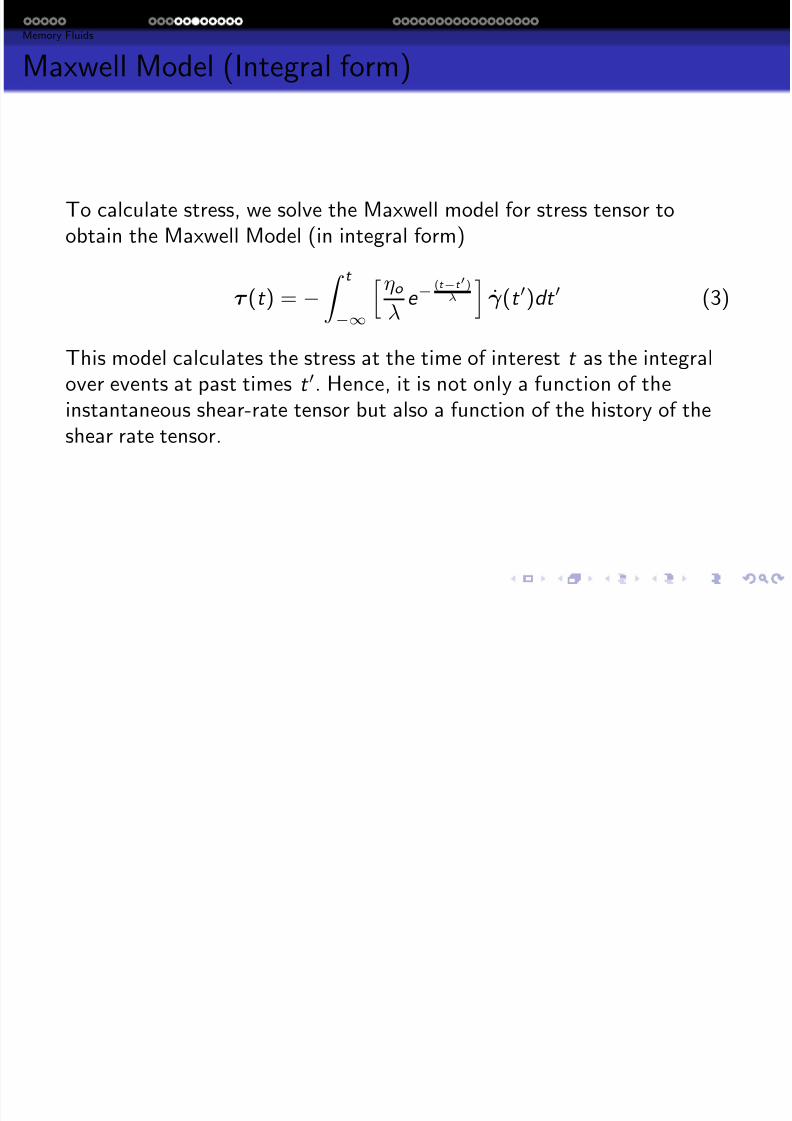
Maxwell Model (Integral form)
To calculate stress, we solve the Maxwell model for stress tensor toobtain the Maxwell Model (in integral form)
τ (t ) = −
t
−∞
ηo
λ e −
(t −t )λ
γ̇ (t )dt (3)
This model calculates the stress at the time of interest t as the integralover events at past times t . Hence, it is not only a function of the
instantaneous shear-rate tensor but also a function of the history of theshear rate tensor.
Viscoelastic Fluids Mathematical Models of Viscoelastic Flows Numerical Methods of Viscoelastic Flow Simulations Preliminary Results
7/21/2019 Dept Fall2013
http://slidepdf.com/reader/full/dept-fall2013 15/57
Memory Fluids
What Next?
During Modeling of any process, it is always prudent to begin with thesimplest models (i.e. linear models like the previous ones) and to move tomore complex, non-linear equations only if the linear equations areinadequate.
Viscoelastic Fluids Mathematical Models of Viscoelastic Flows Numerical Methods of Viscoelastic Flow Simulations Preliminary Results
7/21/2019 Dept Fall2013
http://slidepdf.com/reader/full/dept-fall2013 16/57
Memory Fluids
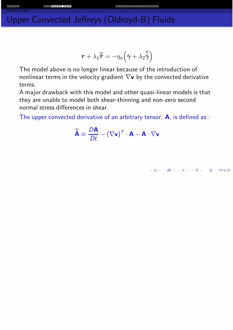
Upper Convected Jeffreys (Oldroyd-B) Fluids
τ + λ1∇
τ = −ηo
γ̇ + λ2
∇
γ̇
The model above is no longer linear because of the introduction of nonlinear terms in the velocity gradient ∇v by the convected derivative
terms.A major drawback with this model and other quasi-linear models is thatthey are unable to model both shear-thinning and non-zero secondnormal stress differences in shear.
The upper convected derivative of an arbitrary tensor, A, is defined as :
∇
A ≡ D A
Dt − (∇v)T · A − A · ∇v
Viscoelastic Fluids Mathematical Models of Viscoelastic Flows Numerical Methods of Viscoelastic Flow Simulations Preliminary Results
7/21/2019 Dept Fall2013
http://slidepdf.com/reader/full/dept-fall2013 17/57
Memory Fluids
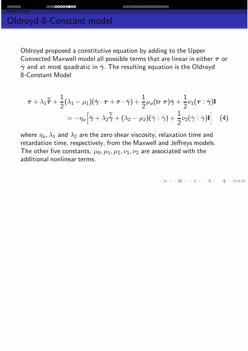
Oldroyd 8-Constant model
Oldroyd proposed a constitutive equation by adding to the UpperConvected Maxwell model all possible terms that are linear in either τ orγ̇ and at most quadratic in γ̇ . The resulting equation is the Oldroyd8-Constant Model
τ + λ1∇
τ + 1
2(λ1 − µ1)(γ̇ · τ + τ · γ̇ ) +
1
2µo (tr τ )γ̇ +
1
2ν 1(τ : γ̇ )I
= −ηo
γ̇ + λ2
∇
γ̇ + (λ2 − µ2)(γ̇ : γ̇ ) + 1
2ν 2(γ̇ : γ̇ )I
(4)
where ηo , λ1 and λ2 are the zero shear viscosity, relaxation time andretardation time, respectively, from the Maxwell and Jeffreys models.The other five constants, µ0, µ1, µ2, ν 1, ν 2 are associated with theadditional nonlinear terms.
Viscoelastic Fluids Mathematical Models of Viscoelastic Flows Numerical Methods of Viscoelastic Flow Simulations Preliminary Results
7/21/2019 Dept Fall2013
http://slidepdf.com/reader/full/dept-fall2013 18/57
Memory Fluids
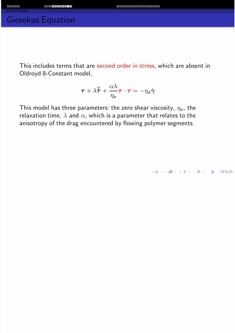
Giesekus Equation
This includes terms that are second order in stress, which are absent inOldroyd 8-Constant model,
τ + λ∇
τ + αλ
ηo
τ · τ = −ηo γ̇
This model has three parameters: the zero shear viscosity, ηo , therelaxation time, λ and α, which is a parameter that relates to the
anisotropy of the drag encountered by flowing polymer segments.
Viscoelastic Fluids Mathematical Models of Viscoelastic Flows Numerical Methods of Viscoelastic Flow Simulations Preliminary Results
7/21/2019 Dept Fall2013
http://slidepdf.com/reader/full/dept-fall2013 19/57
Memory Fluids
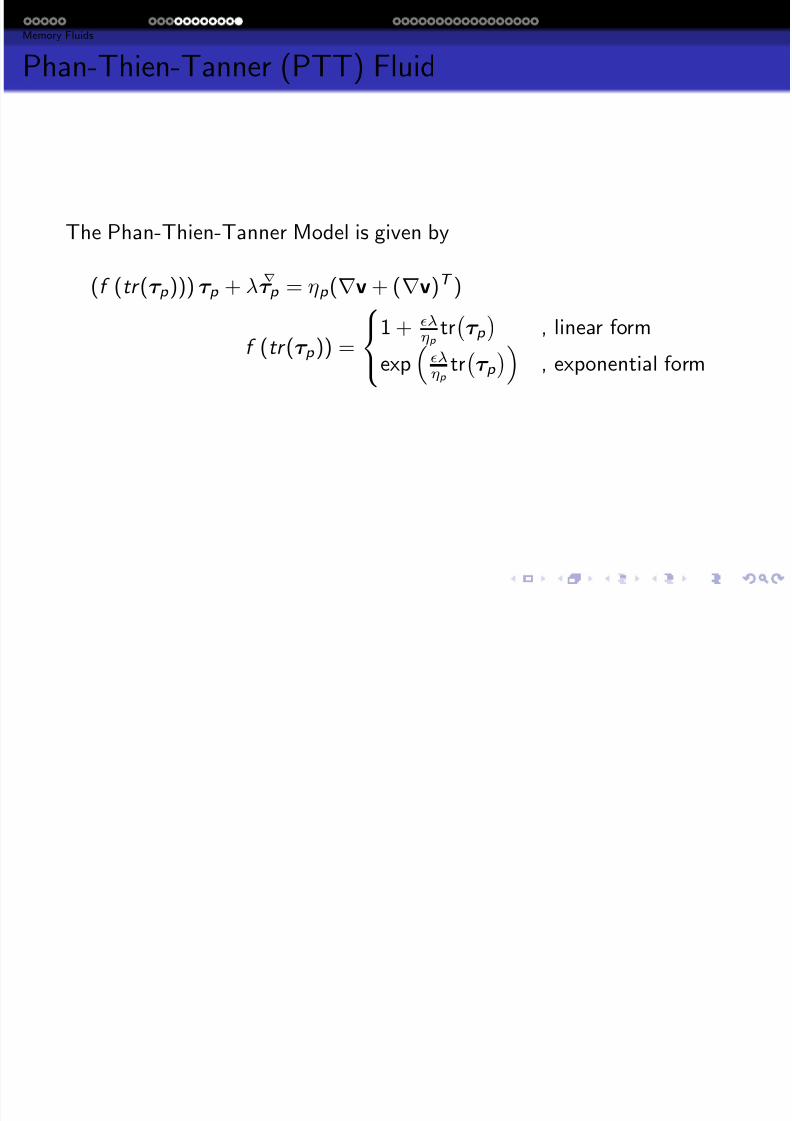
Phan-Thien-Tanner (PTT) Fluid
The Phan-Thien-Tanner Model is given by
(f (tr (τ p ))) τ p + λ∇
τ p = ηp (∇v + (∇v)T )
f (tr (τ p )) =
1 + ληp
trτ p
, linear form
exp
ληp
trτ p
, exponential form
Viscoelastic Fluids Mathematical Models of Viscoelastic Flows Numerical Methods of Viscoelastic Flow Simulations Preliminary Results
7/21/2019 Dept Fall2013
http://slidepdf.com/reader/full/dept-fall2013 20/57
Contents
1 Viscoelastic Fluids
Introduction
Flow Behaviour of Viscoelastic Fluids Vs Newtonian Fluids
2 Mathematical Models of Viscoelastic Flows
Conservation Equation of Continuum MechanicsRheology and Constitutive Equations
Memory Fluids
3 Numerical Methods of Viscoelastic Flow Simulations
Governing Equations
Discretization of the Transport Equation
Iterative Solution Algorithm
4 Preliminary Results
Viscoelastic Fluids Mathematical Models of Viscoelastic Flows Numerical Methods of Viscoelastic Flow Simulations Preliminary Results
7/21/2019 Dept Fall2013
http://slidepdf.com/reader/full/dept-fall2013 21/57
Governing Equations
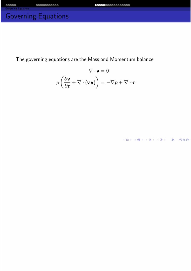
Governing Equations
The governing equations are the Mass and Momentum balance
∇ · v = 0
ρ
∂ v
∂ t + ∇ · (v v)
= −∇p + ∇ · τ
Viscoelastic Fluids Mathematical Models of Viscoelastic Flows Numerical Methods of Viscoelastic Flow Simulations Preliminary Results
7/21/2019 Dept Fall2013
http://slidepdf.com/reader/full/dept-fall2013 22/57
Governing Equations
Governing Equations
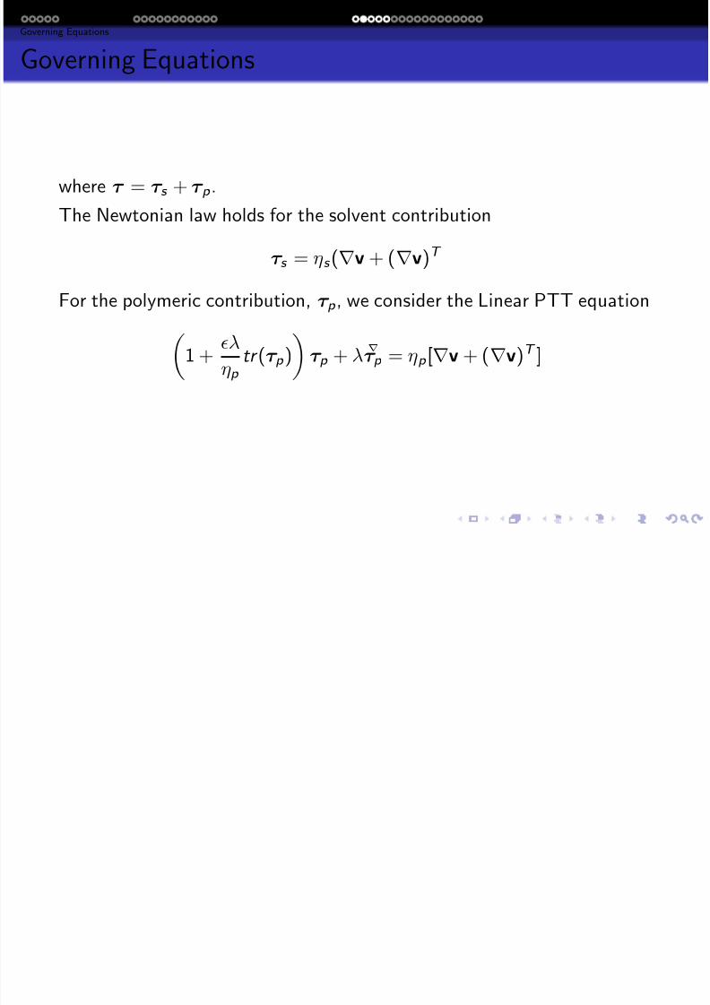
where τ = τ s + τ p .
The Newtonian law holds for the solvent contribution
τ s = ηs (∇v + (∇v)T
For the polymeric contribution, τ p , we consider the Linear PTT equation
1 + λ
ηp
tr (τ p ) τ p + λ∇
τ p = ηp [∇v + (∇v)T ]
Viscoelastic Fluids Mathematical Models of Viscoelastic Flows Numerical Methods of Viscoelastic Flow Simulations Preliminary Results
G
7/21/2019 Dept Fall2013
http://slidepdf.com/reader/full/dept-fall2013 23/57
Governing Equations
High Weissenberg Number Problem (HWNP)
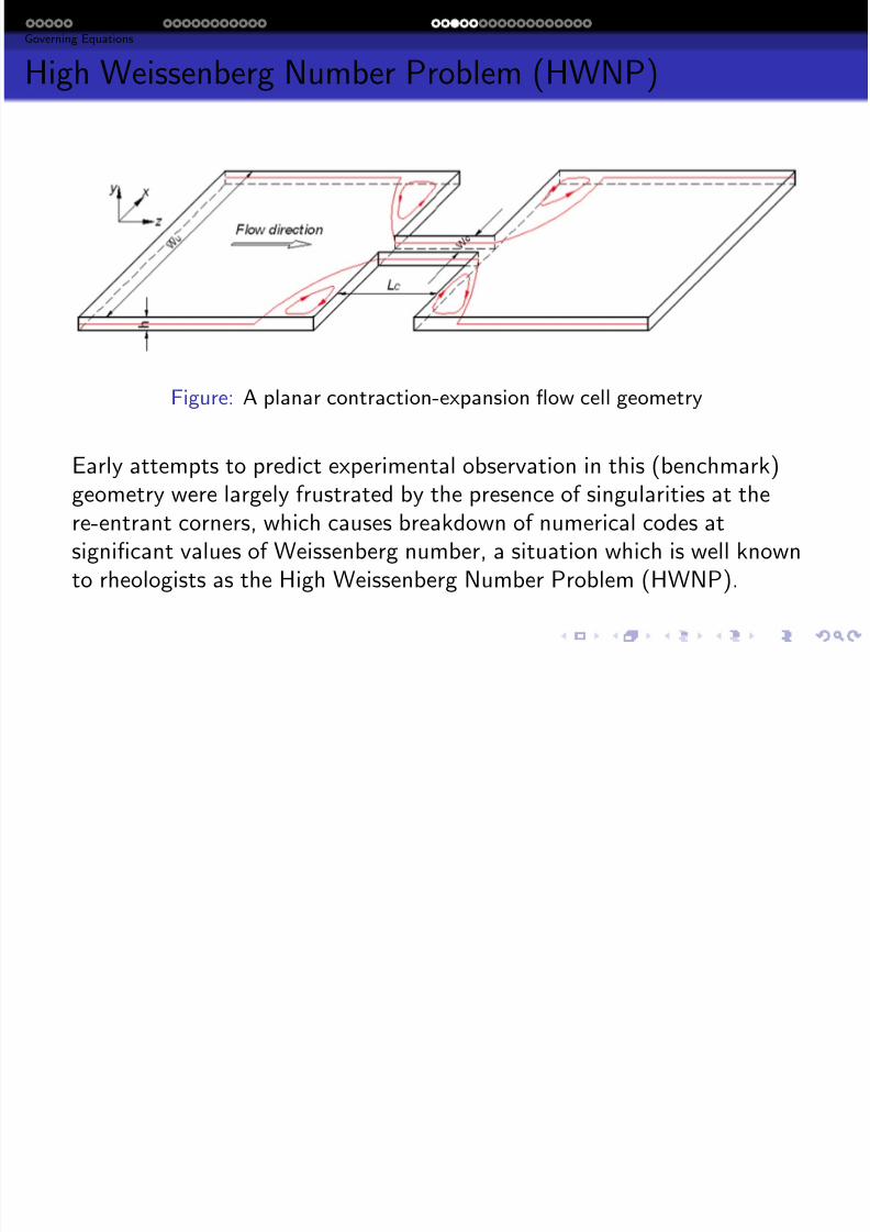
Figure: A planar contraction-expansion flow cell geometry
Early attempts to predict experimental observation in this (benchmark)geometry were largely frustrated by the presence of singularities at there-entrant corners, which causes breakdown of numerical codes atsignificant values of Weissenberg number, a situation which is well knownto rheologists as the High Weissenberg Number Problem (HWNP).
Viscoelastic Fluids Mathematical Models of Viscoelastic Flows Numerical Methods of Viscoelastic Flow Simulations Preliminary Results
G i E ti
7/21/2019 Dept Fall2013
http://slidepdf.com/reader/full/dept-fall2013 24/57
Governing Equations
Stabilization technique (DEVSS)
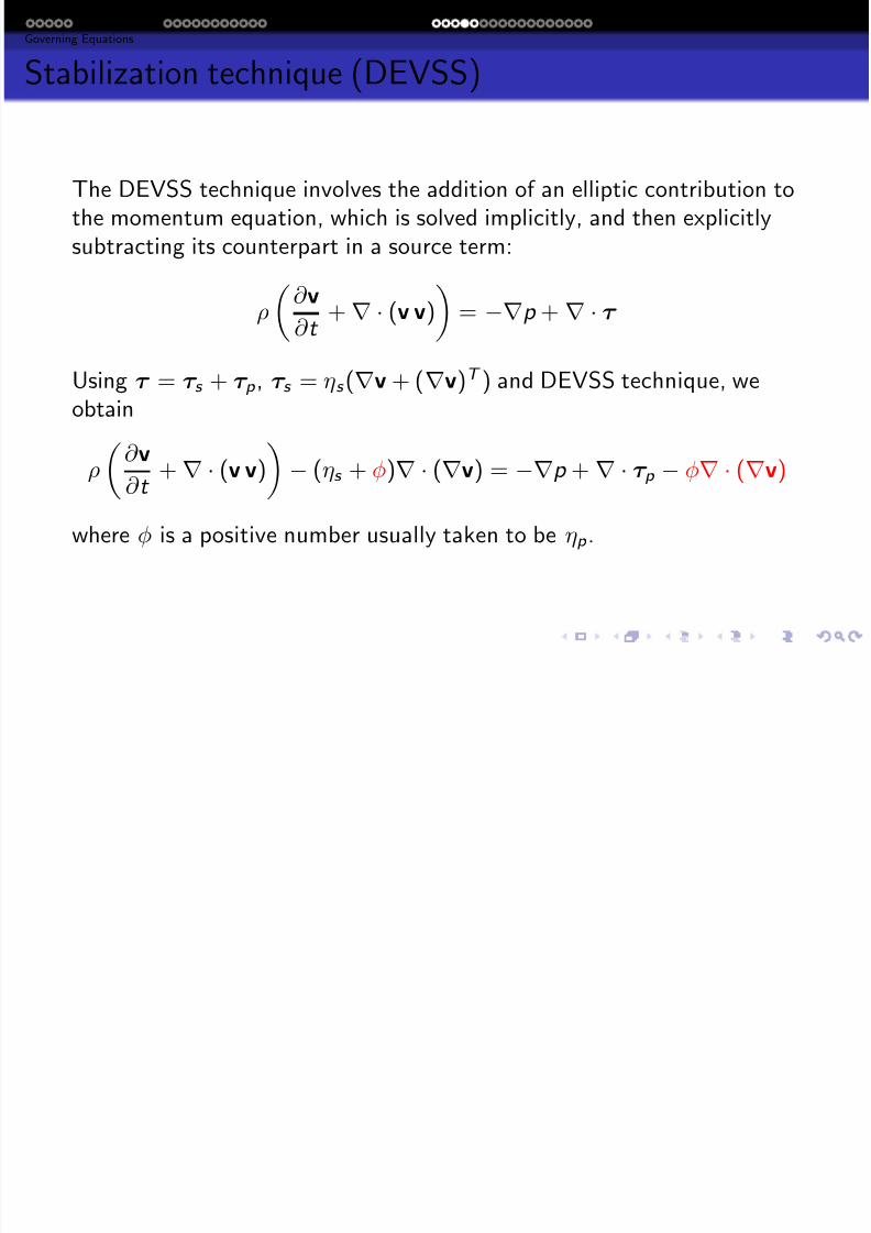
The DEVSS technique involves the addition of an elliptic contribution tothe momentum equation, which is solved implicitly, and then explicitlysubtracting its counterpart in a source term:
ρ∂ v
∂ t + ∇ · (v v)
= −∇p + ∇ · τ
Using τ = τ s + τ p , τ s = ηs (∇v + (∇v)T ) and DEVSS technique, weobtain
ρ
∂ v∂ t + ∇ · (v v)
− (ηs + φ)∇ · (∇v) = −∇p + ∇ · τ p − φ∇ · (∇v)
where φ is a positive number usually taken to be ηp .
Viscoelastic Fluids Mathematical Models of Viscoelastic Flows Numerical Methods of Viscoelastic Flow Simulations Preliminary Results
Governing Equations
7/21/2019 Dept Fall2013
http://slidepdf.com/reader/full/dept-fall2013 25/57
Governing Equations
Stabilization technique (DEVSS)
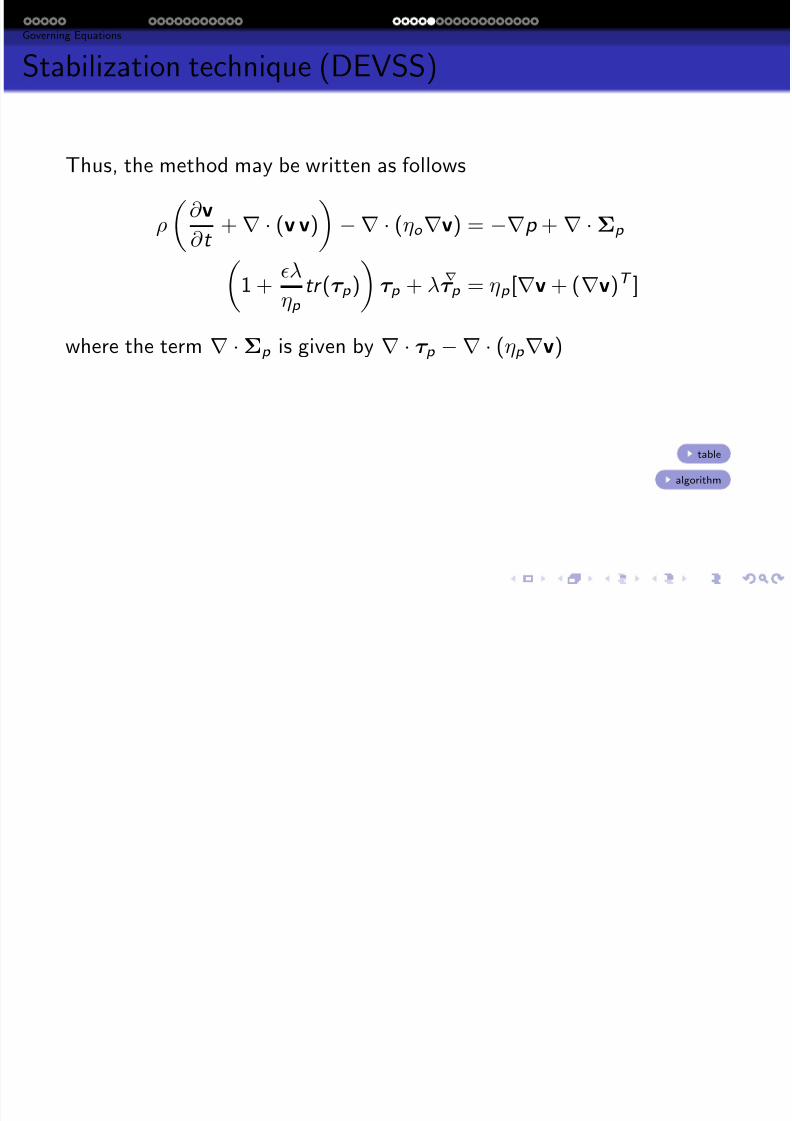
Thus, the method may be written as follows
ρ
∂ v
∂ t + ∇ · (v v)
−∇ · (ηo ∇v) = −∇p + ∇ ·Σp
1 +
λ
ηp tr (τ p )
τ p + λ
∇
τ p = ηp [∇v + (∇v)T ]
where the term ∇ ·Σp is given by ∇ · τ p −∇ · (ηp ∇v)
table
algorithm
Viscoelastic Fluids Mathematical Models of Viscoelastic Flows Numerical Methods of Viscoelastic Flow Simulations Preliminary Results
Discretization of the Transport Equation
7/21/2019 Dept Fall2013
http://slidepdf.com/reader/full/dept-fall2013 26/57
Discretization of the Transport Equation
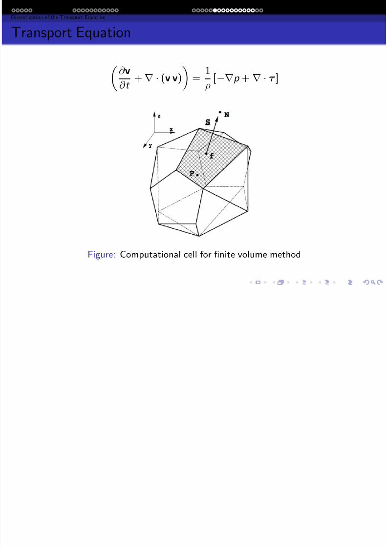
Transport Equation
∂ v∂ t
+ ∇ · (v v)
= 1ρ
[−∇p + ∇ · τ ]
Figure: Computational cell for finite volume method
Viscoelastic Fluids Mathematical Models of Viscoelastic Flows Numerical Methods of Viscoelastic Flow Simulations Preliminary Results
Discretization of the Transport Equation
7/21/2019 Dept Fall2013
http://slidepdf.com/reader/full/dept-fall2013 27/57
Discretization of the Transport Equation
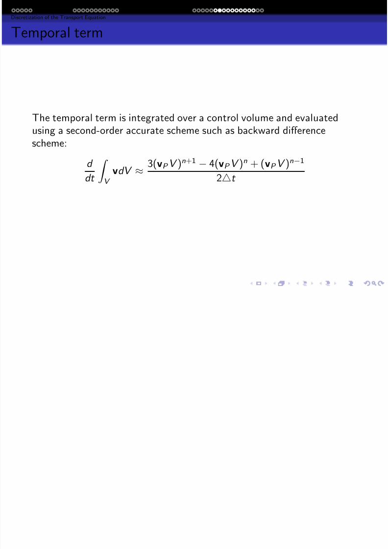
Temporal term
The temporal term is integrated over a control volume and evaluatedusing a second-order accurate scheme such as backward difference
scheme:
d
dt
V
vdV ≈ 3(vP V )n+1 − 4(vP V )n + (vP V )n−1
2t
Viscoelastic Fluids Mathematical Models of Viscoelastic Flows Numerical Methods of Viscoelastic Flow Simulations Preliminary Results
Discretization of the Transport Equation
7/21/2019 Dept Fall2013
http://slidepdf.com/reader/full/dept-fall2013 28/57
Discretization of the Transport Equation
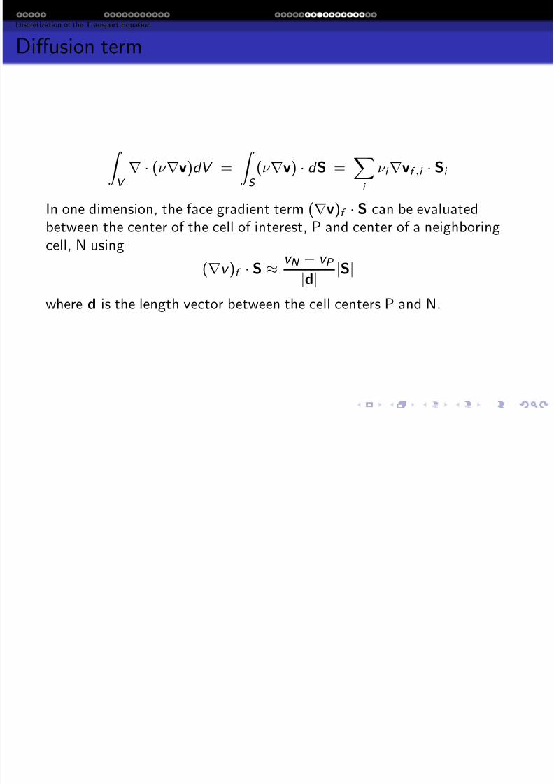
Diffusion term
V
∇ · (ν ∇v)dV =
S
(ν ∇v) · d S =
i ν i ∇vf ,i · Si
In one dimension, the face gradient term (∇v)f · S can be evaluatedbetween the center of the cell of interest, P and center of a neighboringcell, N using
(∇v )f · S ≈ v N − v P
|d| |S|
where d is the length vector between the cell centers P and N.
Viscoelastic Fluids Mathematical Models of Viscoelastic Flows Numerical Methods of Viscoelastic Flow Simulations Preliminary Results
Discretization of the Transport Equation
7/21/2019 Dept Fall2013
http://slidepdf.com/reader/full/dept-fall2013 29/57
p q
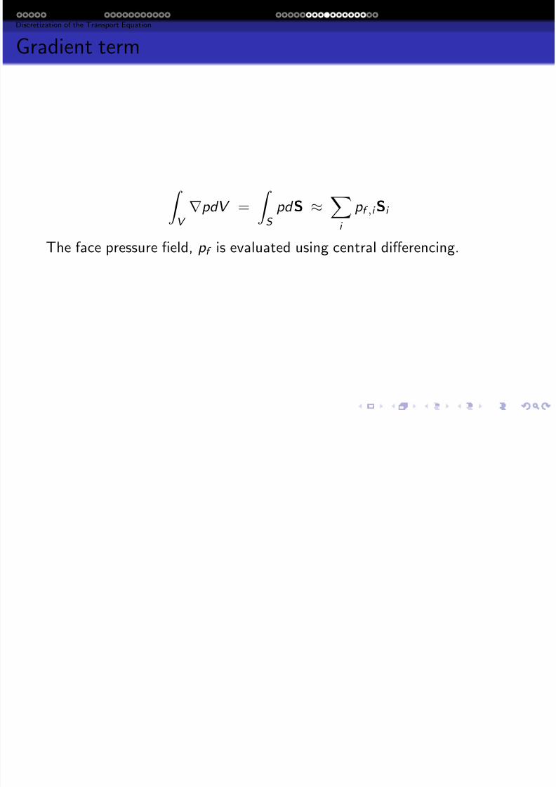
Gradient term
V
∇pdV = S
pd S ≈i
p f ,i Si
The face pressure field, p f is evaluated using central differencing.
Viscoelastic Fluids Mathematical Models of Viscoelastic Flows Numerical Methods of Viscoelastic Flow Simulations Preliminary Results
Discretization of the Transport Equation
7/21/2019 Dept Fall2013
http://slidepdf.com/reader/full/dept-fall2013 30/57
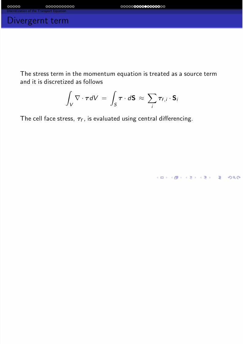
Divergernt term
The stress term in the momentum equation is treated as a source termand it is discretized as follows
V
∇ · τ dV =
S
τ · d S ≈i
τ f ,i · Si
The cell face stress, τ f , is evaluated using central differencing.
Viscoelastic Fluids Mathematical Models of Viscoelastic Flows Numerical Methods of Viscoelastic Flow Simulations Preliminary Results
Discretization of the Transport Equation
7/21/2019 Dept Fall2013
http://slidepdf.com/reader/full/dept-fall2013 31/57
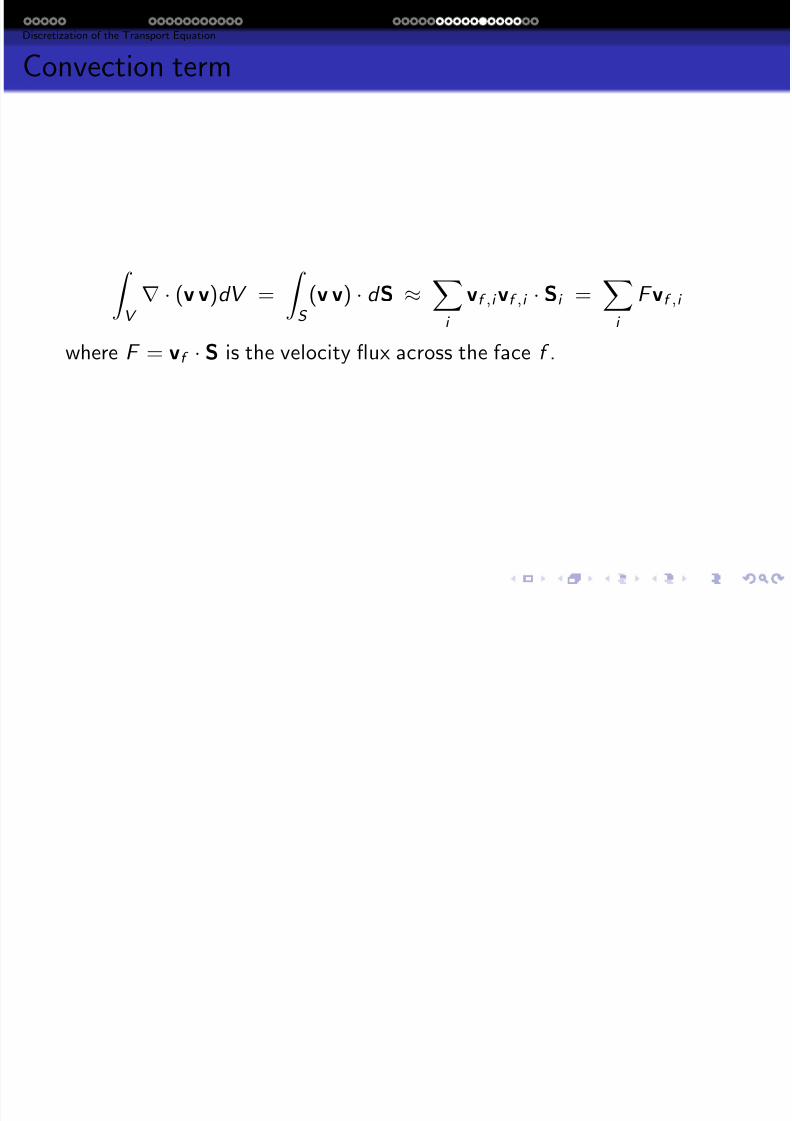
Convection term
V
∇ · (v v)dV = S
(v v) · d S ≈i
vf ,i vf ,i · Si =i
F vf ,i
where F = vf · S is the velocity flux across the face f .
Viscoelastic Fluids Mathematical Models of Viscoelastic Flows Numerical Methods of Viscoelastic Flow Simulations Preliminary Results
Discretization of the Transport Equation
7/21/2019 Dept Fall2013
http://slidepdf.com/reader/full/dept-fall2013 32/57
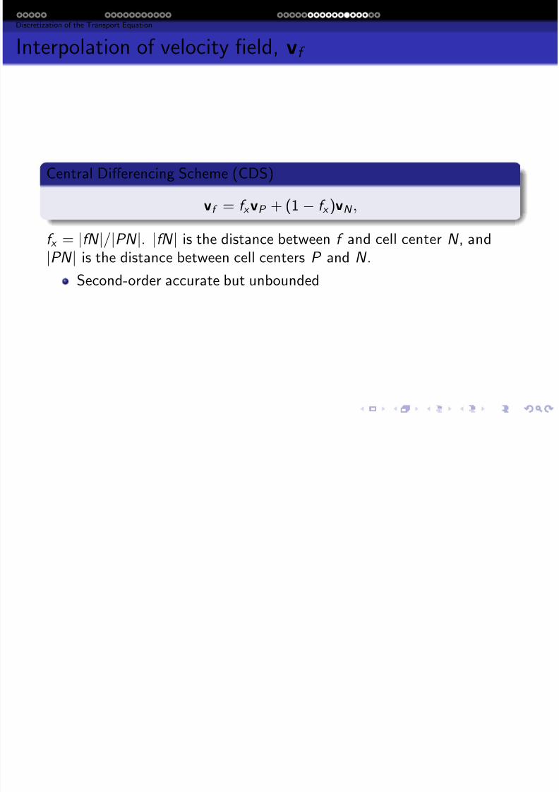
Interpolation of velocity field, vf
Central Differencing Scheme (CDS)
vf = f x vP + (1 − f x )vN ,
f x = |fN |/|PN |. |fN | is the distance between f and cell center N , and|PN | is the distance between cell centers P and N .
Second-order accurate but unbounded
Viscoelastic Fluids Mathematical Models of Viscoelastic Flows Numerical Methods of Viscoelastic Flow Simulations Preliminary Results
Discretization of the Transport Equation
7/21/2019 Dept Fall2013
http://slidepdf.com/reader/full/dept-fall2013 33/57
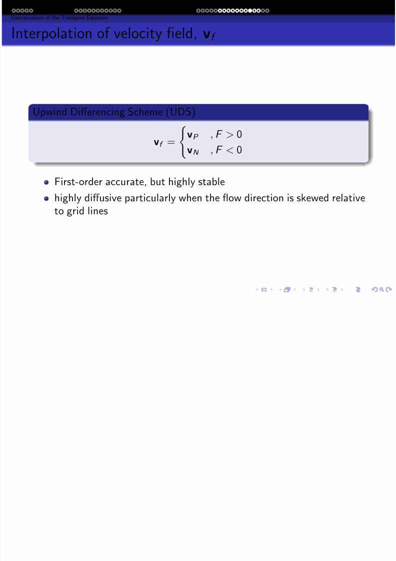
Interpolation of velocity field, vf
Upwind Differencing Scheme (UDS)
vf =vP , F > 0
vN , F < 0
First-order accurate, but highly stable
highly diffusive particularly when the flow direction is skewed relative
to grid lines
Viscoelastic Fluids Mathematical Models of Viscoelastic Flows Numerical Methods of Viscoelastic Flow Simulations Preliminary Results
Discretization of the Transport Equation
7/21/2019 Dept Fall2013
http://slidepdf.com/reader/full/dept-fall2013 34/57
Minmod Scheme (Roe (1985))
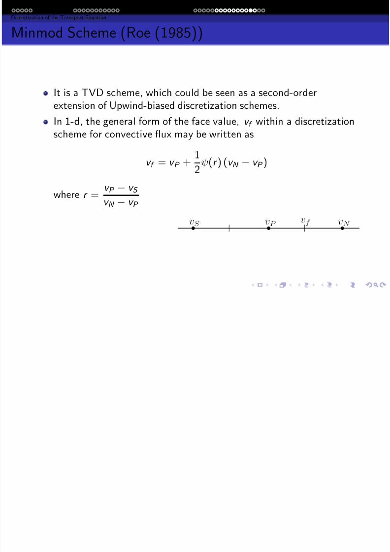
It is a TVD scheme, which could be seen as a second-orderextension of Upwind-biased discretization schemes.
In 1-d, the general form of the face value, v f within a discretizationscheme for convective flux may be written as
v f = v P + 1
2ψ(r ) (v N − v P )
where r = v P − v S
v N − v P
Viscoelastic Fluids Mathematical Models of Viscoelastic Flows Numerical Methods of Viscoelastic Flow Simulations Preliminary Results
Discretization of the Transport Equation
7/21/2019 Dept Fall2013
http://slidepdf.com/reader/full/dept-fall2013 35/57
Minmod Scheme (Roe (1985))
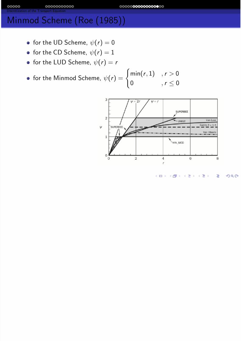
for the UD Scheme, ψ(r ) = 0for the CD Scheme, ψ(r ) = 1
for the LUD Scheme, ψ(r ) = r
for the Minmod Scheme, ψ(r ) = min(r , 1) , r > 0
0 , r ≤ 0
Viscoelastic Fluids Mathematical Models of Viscoelastic Flows Numerical Methods of Viscoelastic Flow Simulations Preliminary Results
Iterative Solution Algorithm
7/21/2019 Dept Fall2013
http://slidepdf.com/reader/full/dept-fall2013 36/57
Iterative Solution Algorithm
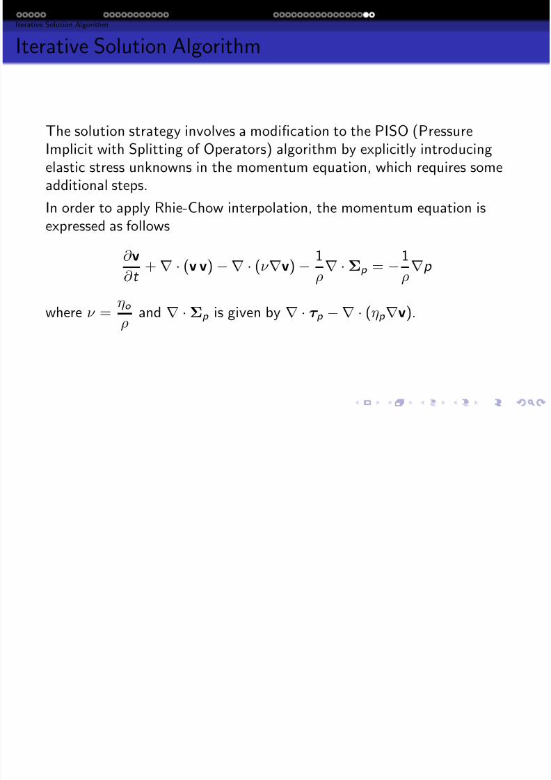
The solution strategy involves a modification to the PISO (PressureImplicit with Splitting of Operators) algorithm by explicitly introducingelastic stress unknowns in the momentum equation, which requires someadditional steps.
In order to apply Rhie-Chow interpolation, the momentum equation isexpressed as follows
∂ v
∂ t + ∇ · (v v) −∇ · (ν ∇v) −
1
ρ∇ ·Σp = −
1
ρ∇p
where ν = ηo
ρ and ∇ ·Σp is given by ∇ · τ p −∇ · (ηp ∇v).
Viscoelastic Fluids Mathematical Models of Viscoelastic Flows Numerical Methods of Viscoelastic Flow Simulations Preliminary Results
Iterative Solution Algorithm
7/21/2019 Dept Fall2013
http://slidepdf.com/reader/full/dept-fall2013 37/57
Iterative Solution Algorithm
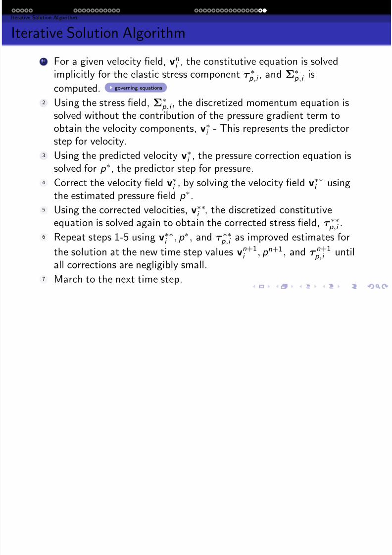
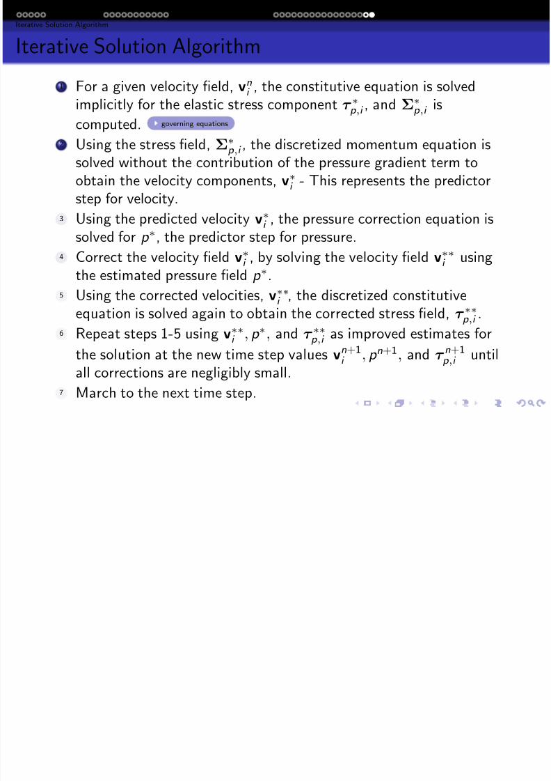
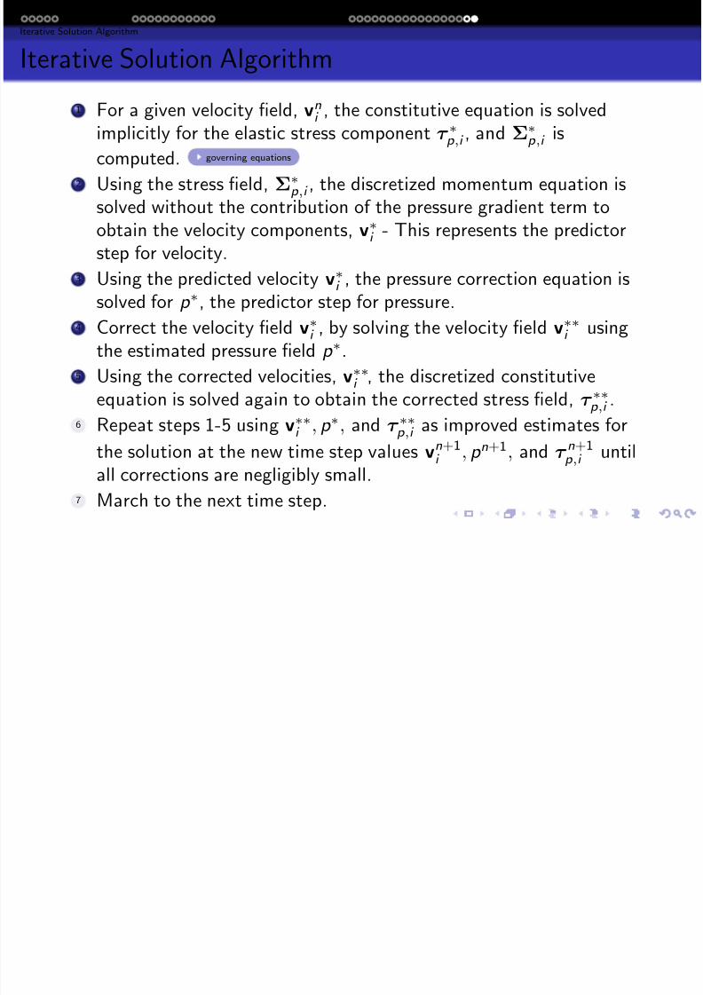
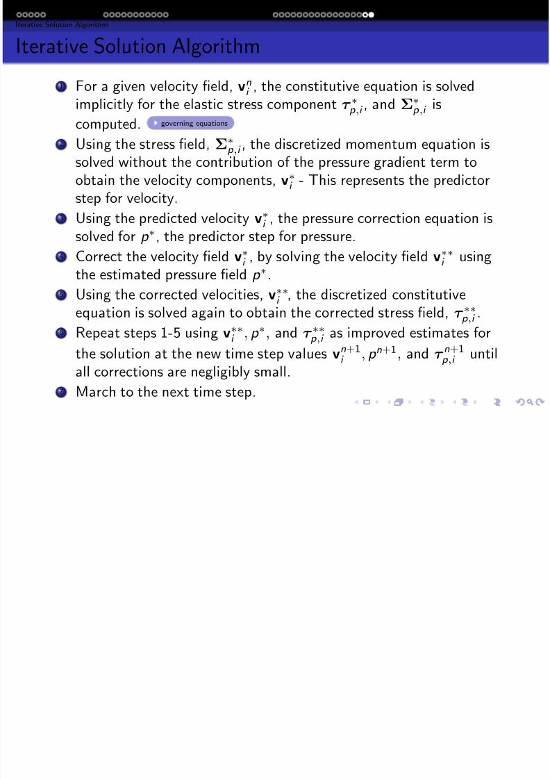
1 For a given velocity field, vni , the constitutive equation is solved
implicitly for the elastic stress component τ ∗
p ,i , and Σ∗
p ,i iscomputed. governing equations
2 Using the stress field, Σ∗
p ,i , the discretized momentum equation issolved without the contribution of the pressure gradient term toobtain the velocity components, v∗i - This represents the predictor
step for velocity.3 Using the predicted velocity v∗i , the pressure correction equation is
solved for p ∗, the predictor step for pressure.4 Correct the velocity field v∗i , by solving the velocity field v∗∗i using
the estimated pressure field p ∗.
5 Using the corrected velocities, v∗∗
i , the discretized constitutiveequation is solved again to obtain the corrected stress field, τ ∗∗p ,i .
6 Repeat steps 1-5 using v∗∗i , p ∗, and τ ∗∗
p ,i as improved estimates for
the solution at the new time step values vn+1i , p n+1, and τ
n+1p ,i until
all corrections are negligibly small.
7 March to the next time step.
Viscoelastic Fluids Mathematical Models of Viscoelastic Flows Numerical Methods of Viscoelastic Flow Simulations Preliminary Results
Iterative Solution Algorithm
7/21/2019 Dept Fall2013
http://slidepdf.com/reader/full/dept-fall2013 38/57
Iterative Solution Algorithm
1 For a given velocity field, vni , the constitutive equation is solved
implicitly for the elastic stress component τ ∗
p ,i , and Σ∗
p ,i iscomputed. governing equations
2 Using the stress field, Σ∗
p ,i , the discretized momentum equation issolved without the contribution of the pressure gradient term toobtain the velocity components, v∗i - This represents the predictor
step for velocity.3 Using the predicted velocity v∗i , the pressure correction equation is
solved for p ∗, the predictor step for pressure.4 Correct the velocity field v∗i , by solving the velocity field v∗∗i using
the estimated pressure field p ∗.
5 Using the corrected velocities, v∗∗
i , the discretized constitutiveequation is solved again to obtain the corrected stress field, τ ∗∗p ,i .
6 Repeat steps 1-5 using v∗∗i , p ∗, and τ ∗∗
p ,i as improved estimates for
the solution at the new time step values vn+1i , p n+1, and τ
n+1p ,i until
all corrections are negligibly small.
7 March to the next time step.
Viscoelastic Fluids Mathematical Models of Viscoelastic Flows Numerical Methods of Viscoelastic Flow Simulations Preliminary Results
Iterative Solution Algorithm
I S l Al h

7/21/2019 Dept Fall2013
http://slidepdf.com/reader/full/dept-fall2013 39/57
Iterative Solution Algorithm
1 For a given velocity field, vni , the constitutive equation is solved
implicitly for the elastic stress component τ ∗
p ,i , and Σ∗
p ,i iscomputed. governing equations
2 Using the stress field, Σ∗
p ,i , the discretized momentum equation issolved without the contribution of the pressure gradient term toobtain the velocity components, v∗i - This represents the predictor
step for velocity.3 Using the predicted velocity v∗i , the pressure correction equation is
solved for p ∗, the predictor step for pressure.4 Correct the velocity field v∗i , by solving the velocity field v∗∗i using
the estimated pressure field p ∗.
5 Using the corrected velocities, v∗∗
i , the discretized constitutiveequation is solved again to obtain the corrected stress field, τ ∗∗p ,i .
6 Repeat steps 1-5 using v∗∗i , p ∗, and τ ∗∗
p ,i as improved estimates for
the solution at the new time step values vn+1i , p n+1, and τ
n+1p ,i until
all corrections are negligibly small.
7 March to the next time step.
Viscoelastic Fluids Mathematical Models of Viscoelastic Flows Numerical Methods of Viscoelastic Flow Simulations Preliminary Results
Iterative Solution Algorithm
I i S l i Al i h

7/21/2019 Dept Fall2013
http://slidepdf.com/reader/full/dept-fall2013 40/57
Iterative Solution Algorithm
1 For a given velocity field, vni , the constitutive equation is solved
implicitly for the elastic stress component τ ∗
p ,i , and Σ∗
p ,i iscomputed. governing equations
2 Using the stress field, Σ∗
p ,i , the discretized momentum equation issolved without the contribution of the pressure gradient term toobtain the velocity components, v∗i - This represents the predictor
step for velocity.3 Using the predicted velocity v∗i , the pressure correction equation is
solved for p ∗, the predictor step for pressure.4 Correct the velocity field v∗i , by solving the velocity field v∗∗i using
the estimated pressure field p ∗.
5 Using the corrected velocities, v∗∗
i , the discretized constitutiveequation is solved again to obtain the corrected stress field, τ ∗∗p ,i .
6 Repeat steps 1-5 using v∗∗i , p ∗, and τ ∗∗
p ,i as improved estimates for
the solution at the new time step values vn+1i , p n+1, and τ
n+1p ,i until
all corrections are negligibly small.
7 March to the next time step.
Viscoelastic Fluids Mathematical Models of Viscoelastic Flows Numerical Methods of Viscoelastic Flow Simulations Preliminary Results
Iterative Solution Algorithm
I i S l i Al i h
7/21/2019 Dept Fall2013
http://slidepdf.com/reader/full/dept-fall2013 41/57
Iterative Solution Algorithm
1 For a given velocity field, vni , the constitutive equation is solved
implicitly for the elastic stress component τ ∗
p ,i , and Σ∗
p ,i iscomputed. governing equations
2 Using the stress field, Σ∗
p ,i , the discretized momentum equation issolved without the contribution of the pressure gradient term toobtain the velocity components, v∗i - This represents the predictor
step for velocity.3 Using the predicted velocity v∗i , the pressure correction equation is
solved for p ∗, the predictor step for pressure.4 Correct the velocity field v∗i , by solving the velocity field v∗∗i using
the estimated pressure field p ∗.
5 Using the corrected velocities, v∗∗
i , the discretized constitutiveequation is solved again to obtain the corrected stress field, τ ∗∗p ,i .
6 Repeat steps 1-5 using v∗∗i , p ∗, and τ ∗∗
p ,i as improved estimates for
the solution at the new time step values vn+1i , p n+1, and τ
n+1p ,i until
all corrections are negligibly small.
7 March to the next time step.
Viscoelastic Fluids Mathematical Models of Viscoelastic Flows Numerical Methods of Viscoelastic Flow Simulations Preliminary Results
Iterative Solution Algorithm
It ti S l ti Al ith
7/21/2019 Dept Fall2013
http://slidepdf.com/reader/full/dept-fall2013 42/57
Iterative Solution Algorithm
1 For a given velocity field, vni , the constitutive equation is solved
implicitly for the elastic stress component τ ∗
p ,i , and Σ∗
p ,i iscomputed. governing equations
2 Using the stress field, Σ∗
p ,i , the discretized momentum equation issolved without the contribution of the pressure gradient term toobtain the velocity components, v∗i - This represents the predictor
step for velocity.3 Using the predicted velocity v∗i , the pressure correction equation is
solved for p ∗, the predictor step for pressure.4 Correct the velocity field v∗i , by solving the velocity field v∗∗i using
the estimated pressure field p ∗.
5 Using the corrected velocities, v∗∗
i , the discretized constitutiveequation is solved again to obtain the corrected stress field, τ ∗∗p ,i .
6 Repeat steps 1-5 using v∗∗i , p ∗, and τ ∗∗
p ,i as improved estimates for
the solution at the new time step values vn+1i , p n+1, and τ
n+1p ,i until
all corrections are negligibly small.
7 March to the next time step.
Viscoelastic Fluids Mathematical Models of Viscoelastic Flows Numerical Methods of Viscoelastic Flow Simulations Preliminary Results
C t t
7/21/2019 Dept Fall2013
http://slidepdf.com/reader/full/dept-fall2013 43/57
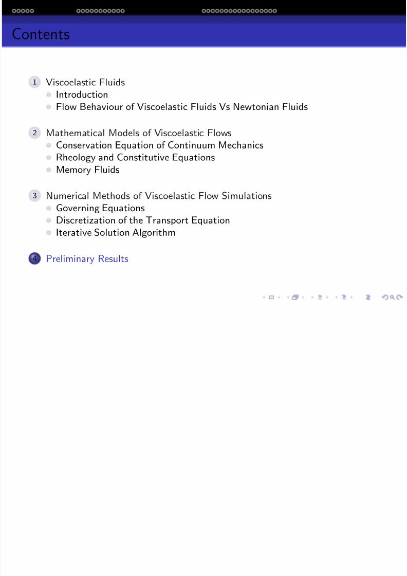
Contents
1 Viscoelastic Fluids
Introduction
Flow Behaviour of Viscoelastic Fluids Vs Newtonian Fluids
2 Mathematical Models of Viscoelastic Flows
Conservation Equation of Continuum MechanicsRheology and Constitutive Equations
Memory Fluids
3 Numerical Methods of Viscoelastic Flow Simulations
Governing Equations
Discretization of the Transport EquationIterative Solution Algorithm
4 Preliminary Results
Viscoelastic Fluids Mathematical Models of Viscoelastic Flows Numerical Methods of Viscoelastic Flow Simulations Preliminary Results
Test Geometry
7/21/2019 Dept Fall2013
http://slidepdf.com/reader/full/dept-fall2013 44/57
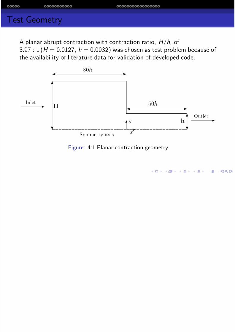
Test Geometry
A planar abrupt contraction with contraction ratio, H /h, of 3.97 : 1 (H = 0.0127, h = 0.0032) was chosen as test problem because of the availability of literature data for validation of developed code.
Figure: 4:1 Planar contraction geometry
Viscoelastic Fluids Mathematical Models of Viscoelastic Flows Numerical Methods of Viscoelastic Flow Simulations Preliminary Results
Flow Properties and Model Parameters
7/21/2019 Dept Fall2013
http://slidepdf.com/reader/full/dept-fall2013 45/57
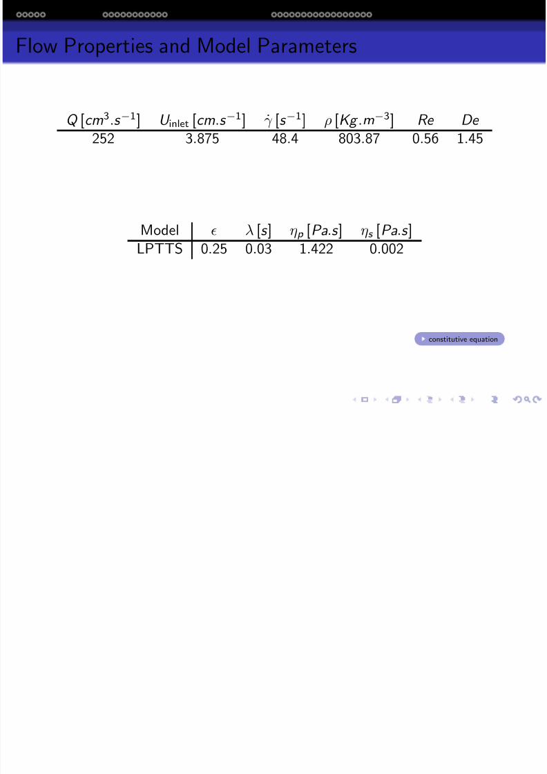
Flow Properties and Model Parameters
Q [cm3.s −1] U inlet [cm.s −1] γ̇ [s −1] ρ [Kg .m−3] Re De
252 3.875 48.4 803.87 0.56 1.45
Model λ [s ] ηp [Pa.s ] ηs [Pa.s ]LPTTS 0.25 0.03 1.422 0.002
constitutive equation
Viscoelastic Fluids Mathematical Models of Viscoelastic Flows Numerical Methods of Viscoelastic Flow Simulations Preliminary Results
Mesh Properties
7/21/2019 Dept Fall2013
http://slidepdf.com/reader/full/dept-fall2013 46/57
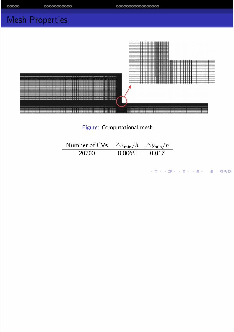
Mesh Properties
Figure: Computational mesh
Number of CVs x min/h y min/h
20700 0.0065 0.017
Viscoelastic Fluids Mathematical Models of Viscoelastic Flows Numerical Methods of Viscoelastic Flow Simulations Preliminary Results
Color Plot of U
7/21/2019 Dept Fall2013
http://slidepdf.com/reader/full/dept-fall2013 47/57
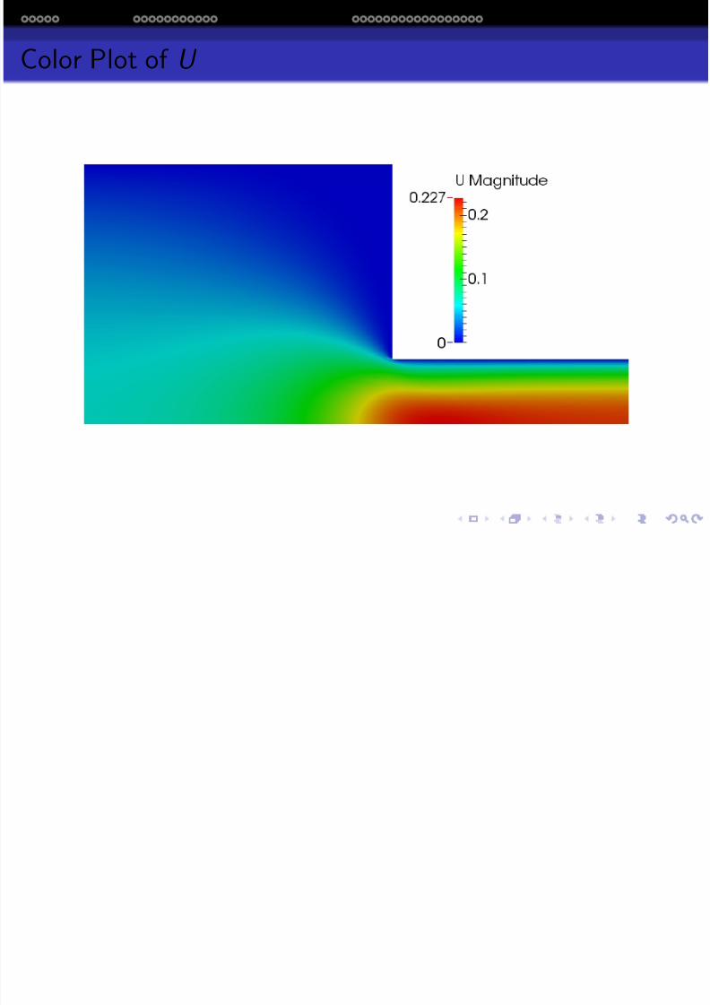
Color Plot of U
Viscoelastic Fluids Mathematical Models of Viscoelastic Flows Numerical Methods of Viscoelastic Flow Simulations Preliminary Results
Streamlines
7/21/2019 Dept Fall2013
http://slidepdf.com/reader/full/dept-fall2013 48/57
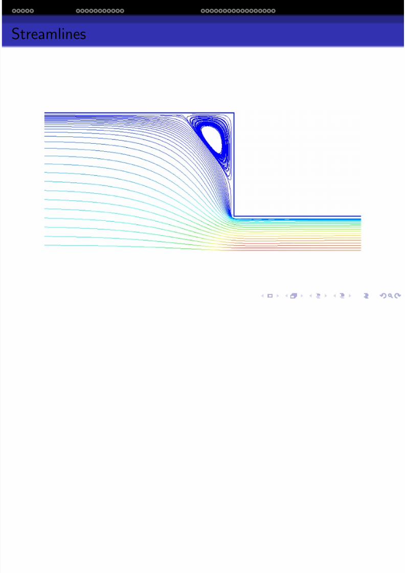
Streamlines
Viscoelastic Fluids Mathematical Models of Viscoelastic Flows Numerical Methods of Viscoelastic Flow Simulations Preliminary Results
Color Plot of τ
7/21/2019 Dept Fall2013
http://slidepdf.com/reader/full/dept-fall2013 49/57
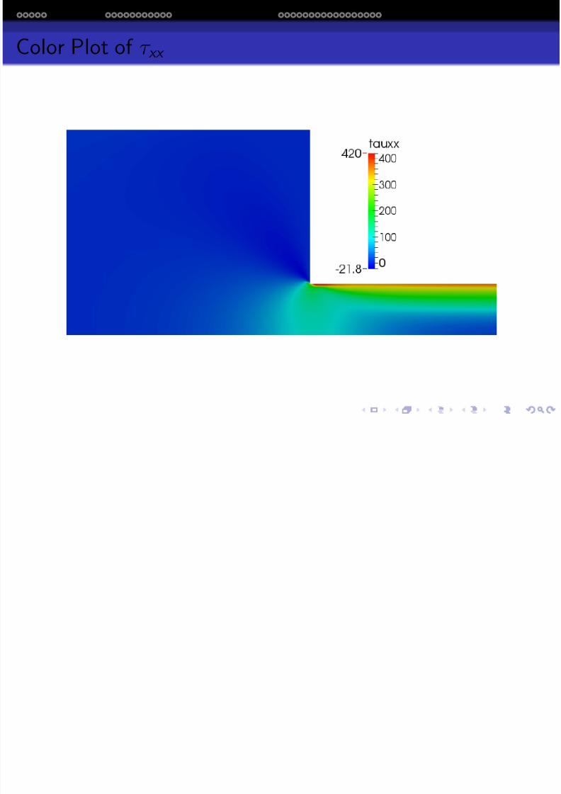
Color Plot of τ xx
Viscoelastic Fluids Mathematical Models of Viscoelastic Flows Numerical Methods of Viscoelastic Flow Simulations Preliminary Results
Velocity profile along centerline for Wi = 1 45
7/21/2019 Dept Fall2013
http://slidepdf.com/reader/full/dept-fall2013 50/57
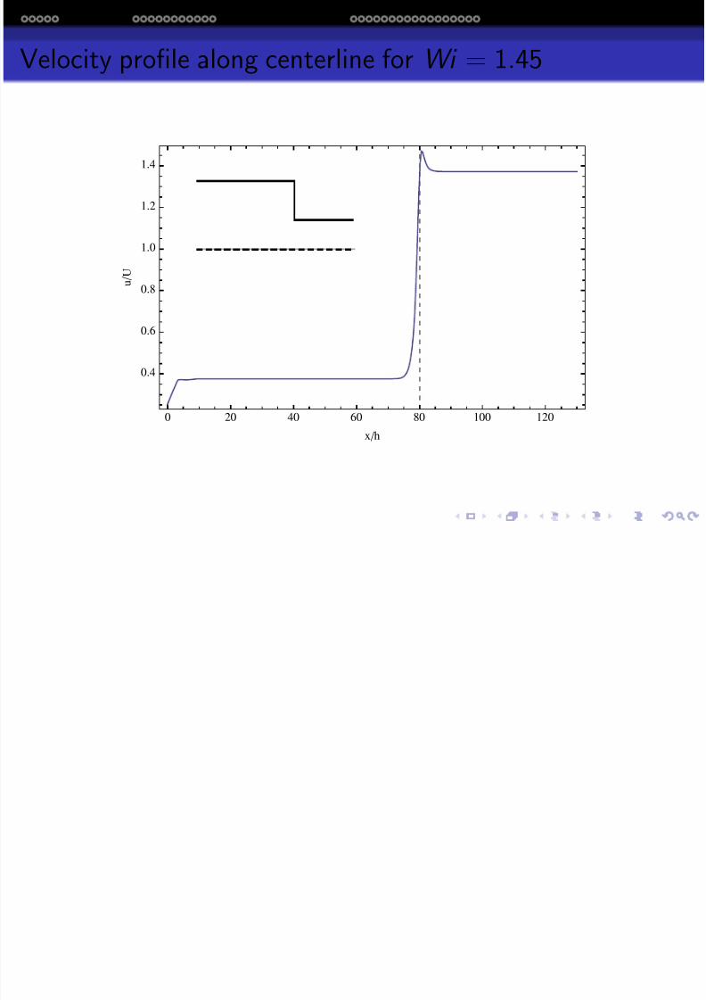
Velocity profile along centerline for Wi = 1.45
0 20 40 60 80 100 120
0.4
0.6
0.8
1.0
1.2
1.4
xh
u U
Viscoelastic Fluids Mathematical Models of Viscoelastic Flows Numerical Methods of Viscoelastic Flow Simulations Preliminary Results
Velocity profiles along centerline for
7/21/2019 Dept Fall2013
http://slidepdf.com/reader/full/dept-fall2013 51/57
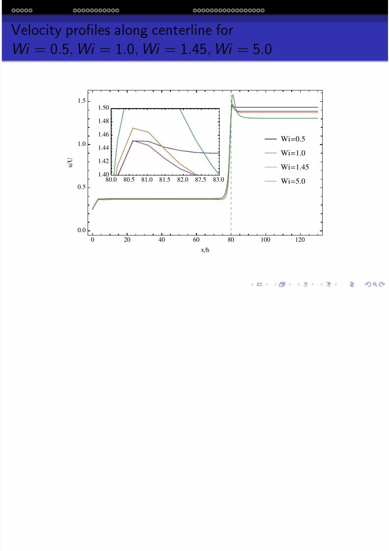
y p gWi = 0.5,Wi = 1.0,Wi = 1.45,Wi = 5.0
Wi0.5
Wi1.0
Wi1.45
Wi5.0
0 20 40 60 80 100 120
0.0
0.5
1.0
1.5
xh
u U
80.0 80.5 81.0 81.5 82.0 82.5 83.01.40
1.42
1.44
1.46
1.48
1.50
Viscoelastic Fluids Mathematical Models of Viscoelastic Flows Numerical Methods of Viscoelastic Flow Simulations Preliminary Results
Velocity profiles on vertical lines in the downstream section
7/21/2019 Dept Fall2013
http://slidepdf.com/reader/full/dept-fall2013 52/57
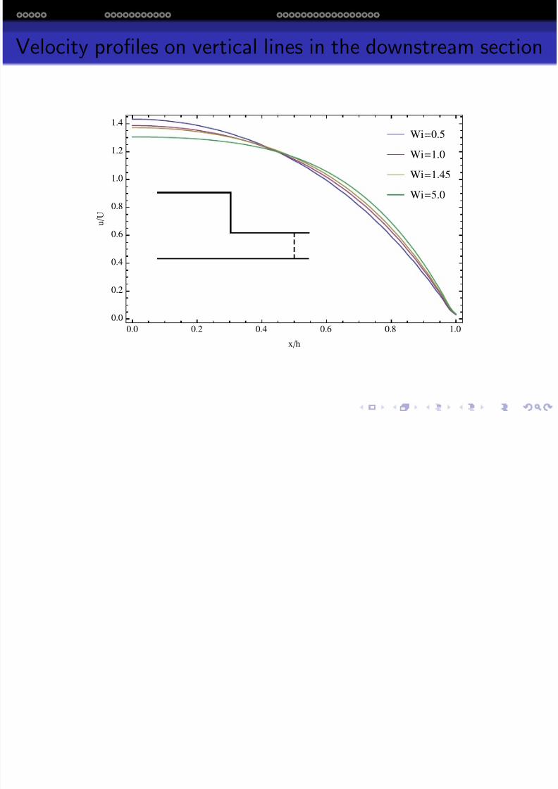
Velocity profiles on vertical lines in the downstream section
Wi0.5
Wi1.0
Wi1.45
Wi5.0
0.0 0.2 0.4 0.6 0.8 1.0
0.0
0.2
0.4
0.6
0.8
1.0
1.2
1.4
xh
u U
Viscoelastic Fluids Mathematical Models of Viscoelastic Flows Numerical Methods of Viscoelastic Flow Simulations Preliminary Results
Conclusion
7/21/2019 Dept Fall2013
http://slidepdf.com/reader/full/dept-fall2013 53/57
Conclusion
The governing equations are discretized using a Collocated finite volumemethod, which has been implemented in the OpenFOAM library:
The convection term of the governing equations is treated usinghigh resolution schemes (e.g. TVD schemes) which provides better
numerical stability and accuracy for hyperbolic PDEs.Further stability was achieved through stress-splitting techniquessuch as DEVSS method, which enhances the elliptic character of thegoverning equations.
The iterative solution strategy is based on the PISO
predictor-corrector algorithm and Rhie-Chow interpolation scheme,which has been modified for Viscoelastic flow calculations.
Viscoelastic Fluids Mathematical Models of Viscoelastic Flows Numerical Methods of Viscoelastic Flow Simulations Preliminary Results
Future Work
7/21/2019 Dept Fall2013
http://slidepdf.com/reader/full/dept-fall2013 54/57
Numerical Simulation of Segmented Two-phase Flows inMicrochannels using Volume of Fluid/ Level Set Method.
Viscoelastic Fluids Mathematical Models of Viscoelastic Flows Numerical Methods of Viscoelastic Flow Simulations Preliminary Results
7/21/2019 Dept Fall2013
http://slidepdf.com/reader/full/dept-fall2013 55/57
Thank You!
Questions, please.
Viscoelastic Fluids Mathematical Models of Viscoelastic Flows Numerical Methods of Viscoelastic Flow Simulations Preliminary Results
Acknowledgements
7/21/2019 Dept Fall2013
http://slidepdf.com/reader/full/dept-fall2013 56/57
g
Viscoelastic Fluids Mathematical Models of Viscoelastic Flows Numerical Methods of Viscoelastic Flow Simulations Preliminary Results
Acknowledgements
7/21/2019 Dept Fall2013
http://slidepdf.com/reader/full/dept-fall2013 57/57
g
Special thanks to the following professors: Dr. Allan Struthers, Dr.
Alexander Labovsky, Dr. Jiguang Sun, Dr. Tamara Olson, Dr.
Zhengfu Xu, Dr. Iosif Pinelis, Dr. Franz Tanner, Dr. Kathleen
Feigl.The great lectures i have been opportuned to take with you havecontributed immensely to this work and would also serve as an impetusfor future projects.The constructive advices given by Prof. Mark Gockenbach has been
invaluable.