Embed Size (px)
Citation preview
Igor Sokolov, Humboldt-Universität zu Berlin
Diffusion in crowded environments:Models, properties, instruments
25th Smoluchowski symposium, Cracow 2012
Igor Sokolov, Humboldt-Universität zu Berlin
Diffusion in crowded environments:Models, properties, instruments
Different stories to tell:
• Normal diffusion• Subdiffusion: Experiments, models, and
mathematical instruments– CTRW– Percolation– Slow modes of multiparticle models
• Aging• Case study 1: REM • Case study 2: “The twins”: exactly solvable examples• Conclusions
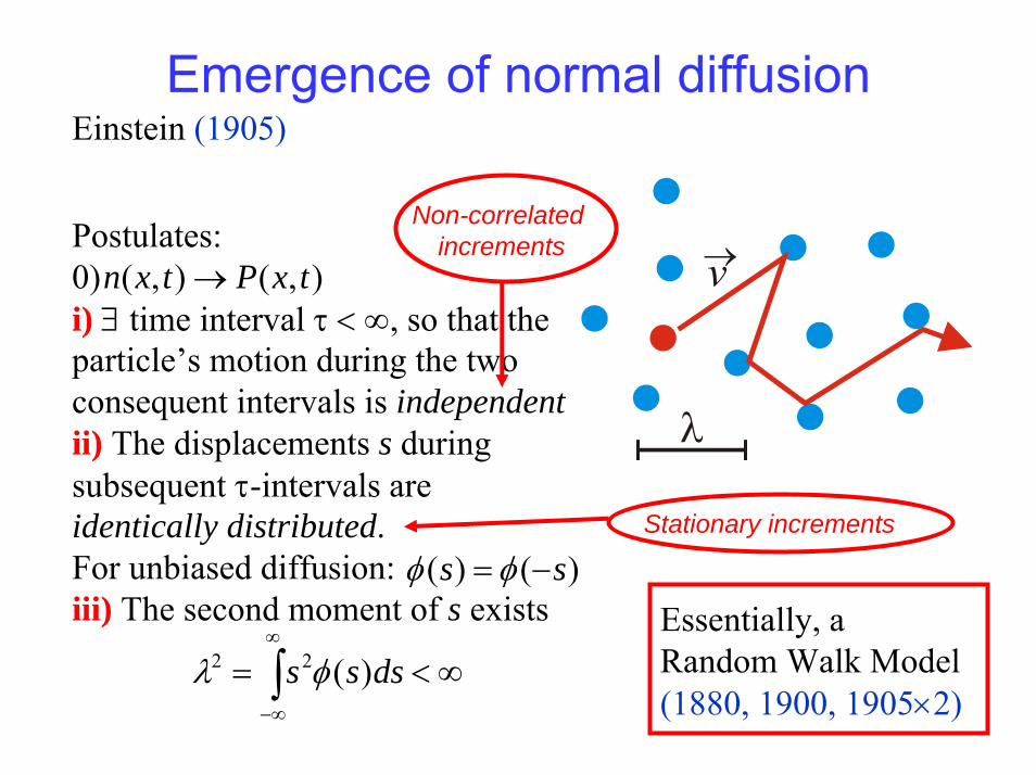
Emergence of normal diffusionEinstein (1905)
Postulates:0)i) ∃ time interval τ < ∞, so that theparticle’s motion during the two consequent intervals is independentii) The displacements s during subsequent τ-intervals are identically distributed. For unbiased diffusion:iii) The second moment of s exists
∞<= ∫∞
∞−
dsss )(22 φλ
)()( ss −= φφ
),(),( txPtxn →
Essentially, a Random Walk Model(1880, 1900, 1905×2)
Stationary increments
Non-correlated increments
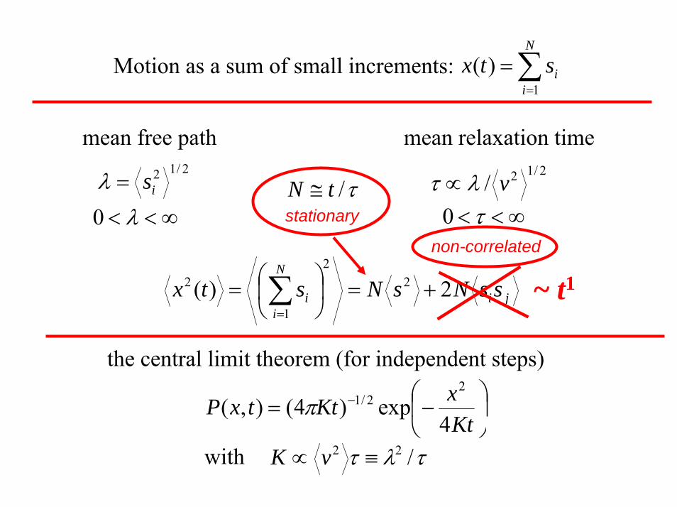
∑=
=N
iistx
1)(Motion as a sum of small increments:
mean relaxation timemean free path2/12
is=λ∞<< λ0
2/12/ vλτ ∝∞<< τ0
τ/tN ≅
ji
N
ii ssNsNstx 2)( 2
2
1
2 +=⎟⎠⎞
⎜⎝⎛= ∑
=~ t1
non-correlated
stationary
the central limit theorem (for independent steps)
⎟⎠
⎞⎜⎝
⎛−= −
KtxKttxP
4exp)4(),(
22/1π
τλτ /22 ≡∝ vKwith
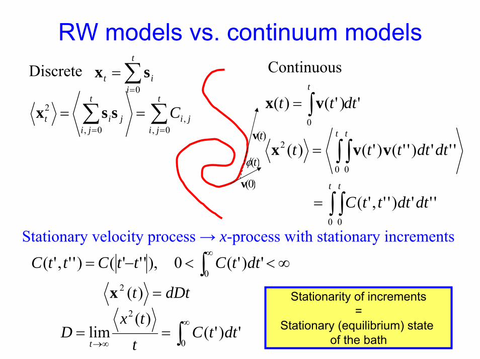
RW models vs. continuum models
∫∞
∞→==
0
2
')'()(
lim dttCttx
Dt
∑∑==
==t
jiji
t
jijit C
0,,
0,
2 ssx
∑=
=t
iit
0sx
')'()(0
dtttt
∫= vx
∫ ∫
∫ ∫
=
=
t t
t t
dtdtttC
dtdtttt
0 0
0 0
2
''')'','(
''')''()'()( vvx
Continuous
Stationary velocity process → x-process with stationary increments
Discrete
∞<<−= ∫∞
0')'(0),'''()'','( dttCttCttC
dDtt =)(2x Stationarity of increments=
Stationary (equilibrium) state of the bath
)(tφ
)(tv
)0(v
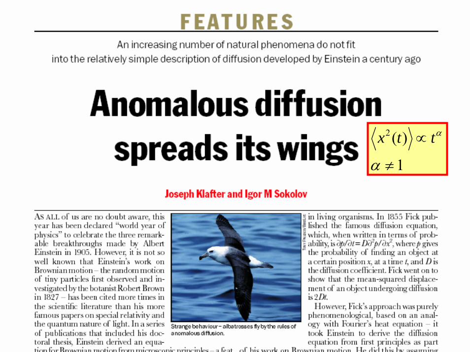
1
)(2
≠
∝
α
αttx
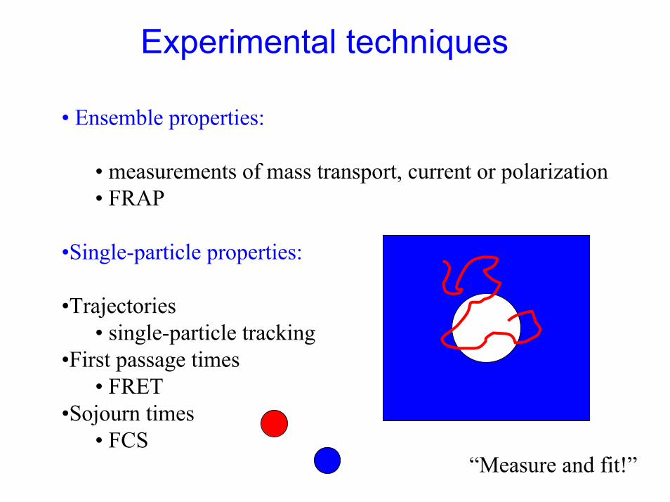
Experimental techniques
• Ensemble properties:
• measurements of mass transport, current or polarization• FRAP
•Single-particle properties:
•Trajectories• single-particle tracking
•First passage times• FRET
•Sojourn times• FCS
“Measure and fit!”
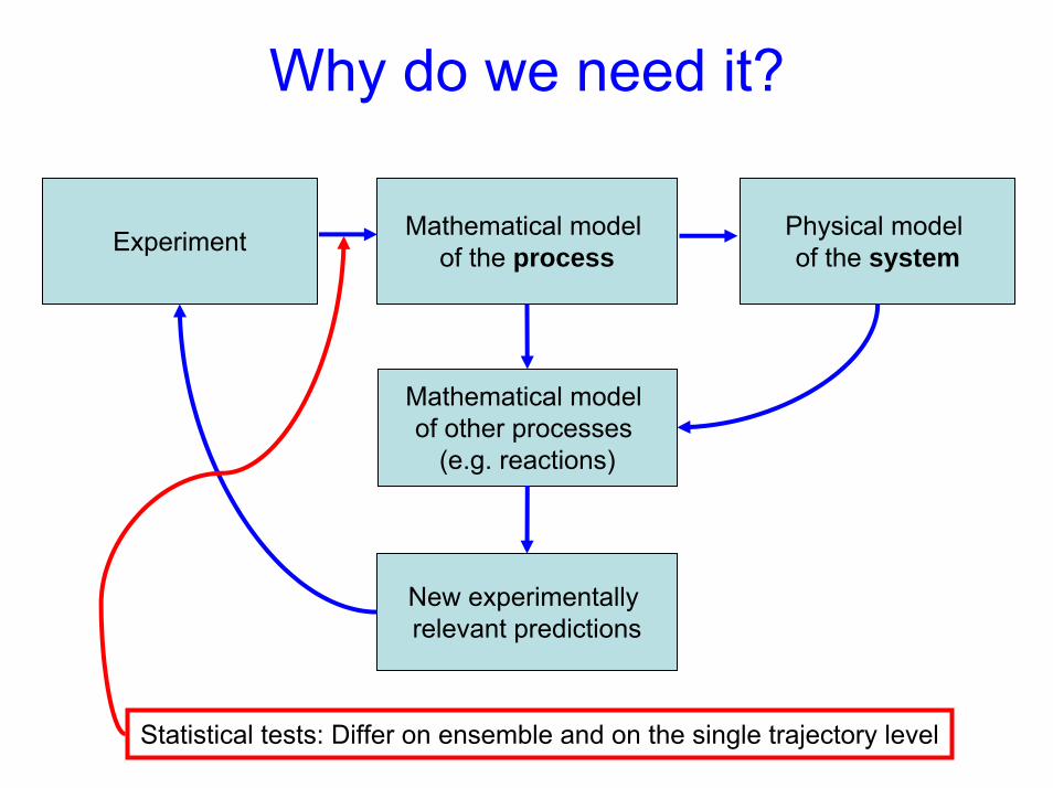
Why do we need it?
Experiment Mathematical model of the process
Physical model of the system
Mathematical model of other processes
(e.g. reactions)
New experimentally relevant predictions
Statistical tests: Differ on ensemble and on the single trajectory level
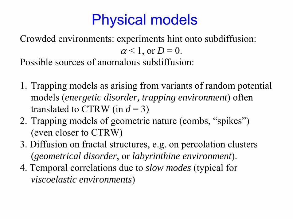
Physical modelsCrowded environments: experiments hint onto subdiffusion:
α < 1, or D = 0.Possible sources of anomalous subdiffusion:
1. Trapping models as arising from variants of random potential models (energetic disorder, trapping environment) often translated to CTRW (in d = 3)
2. Trapping models of geometric nature (combs, “spikes”)(even closer to CTRW)
3. Diffusion on fractal structures, e.g. on percolation clusters(geometrical disorder, or labyrinthine environment).
4. Temporal correlations due to slow modes (typical forviscoelastic environments)
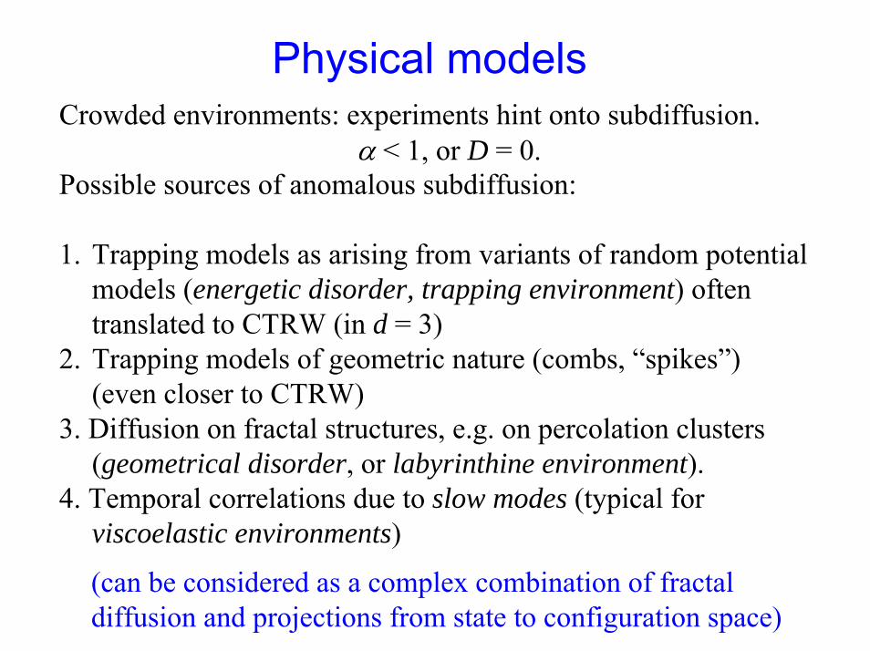
Physical modelsCrowded environments: experiments hint onto subdiffusion.
α < 1, or D = 0.Possible sources of anomalous subdiffusion:
1. Trapping models as arising from variants of random potential models (energetic disorder, trapping environment) often translated to CTRW (in d = 3)
2. Trapping models of geometric nature (combs, “spikes”)(even closer to CTRW)
3. Diffusion on fractal structures, e.g. on percolation clusters(geometrical disorder, or labyrinthine environment).
4. Temporal correlations due to slow modes (typical forviscoelastic environments)
(can be considered as a complex combination of fractal diffusion and projections from state to configuration space)
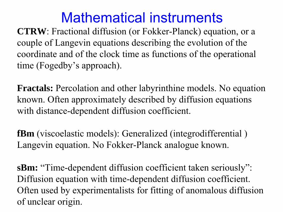
CTRW: Fractional diffusion (or Fokker-Planck) equation, or a couple of Langevin equations describing the evolution of the coordinate and of the clock time as functions of the operationaltime (Fogedby’s approach).
Fractals: Percolation and other labyrinthine models. No equation known. Often approximately described by diffusion equations with distance-dependent diffusion coefficient.
fBm (viscoelastic models): Generalized (integrodifferential ) Langevin equation. No Fokker-Planck analogue known.
sBm: “Time-dependent diffusion coefficient taken seriously”: Diffusion equation with time-dependent diffusion coefficient. Often used by experimentalists for fitting of anomalous diffusion of unclear origin.
Mathematical instruments
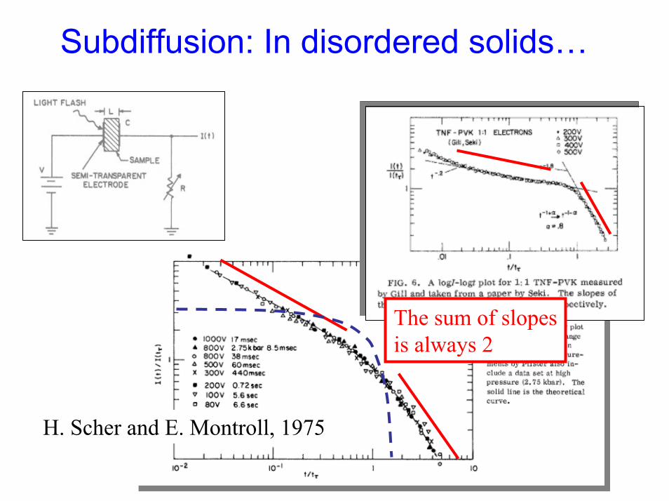
Subdiffusion: In disordered solids…
The sum of slopesis always 2
H. Scher and E. Montroll, 1975
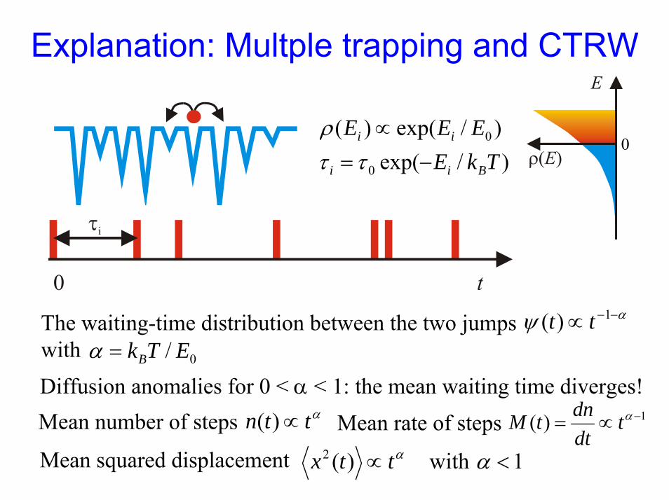
Explanation: Multple trapping and CTRW
)/exp()/exp()(
0
0
TkEEEE
Bii
ii
−=∝
ττρ
0
αψ −−∝ 1)( ttThe waiting-time distribution between the two jumpswith 0/ ETkB=αDiffusion anomalies for 0 < α < 1: the mean waiting time diverges!
Mean squared displacement 1with)(2 <∝ ααttx
Mean rate of steps 1)( −∝= αtdtdntMMean number of steps αttn ∝)(
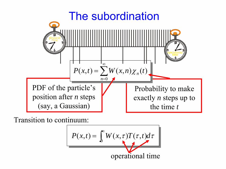
The subordination
PDF of the particle’sposition after n steps
(say, a Gaussian)
Probability to makeexactly n steps up to
the time t
∑∞
=
=0
)(),(),(n
n tnxWtxP χ
Transition to continuum:
τττ dtTxWtxP ∫∞
=0
),(),(),(
operational time
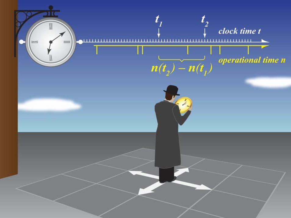
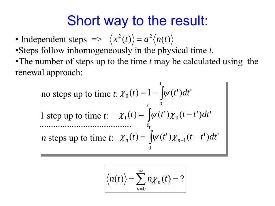
Short way to the result:• Independent steps => •Steps follow inhomogeneously in the physical time t.•The number of steps up to the time t may be calculated using the renewal approach:
∫−=t
dttt0
0 ')'(1)( ψχ
∫ −=t
dttttt0
01 ')'()'()( χψχ........................................
∫ −= −
t
nn dttttt0
1 ')'()'()( χψχ
no steps up to time t:
1 step up to time t:
n steps up to time t:
)()( 22 tnatx =
?)()(0
== ∑∞
=nn tntn χ
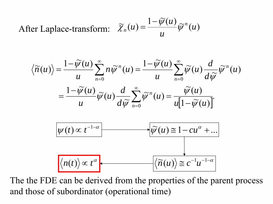
)(~)(~1)(~ uu
uu nn ψψχ −
=After Laplace-transform:
[ ].)(~1)(~
)(~~)(~)(~1
)(~~)(~)(~1)(~)(~1)(~
0
00
∑
∑∑∞
=
∞
=
∞
=
−=
−=
−=
−=
n
n
n
n
n
n
uuuu
ddu
uu
uddu
uuun
uuun
ψψψ
ψψψ
ψψ
ψψψψ
αψ −−∝ 1)( tt ...1)(~ +−≅ αψ cuu
α−−−≅ 11)(~ ucunαttn ∝)(
The the FDE can be derived from the properties of the parent process and those of subordinator (operational time)
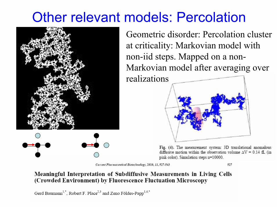
Other relevant models: PercolationGeometric disorder: Percolation cluster at criticality: Markovian model with non-iid steps. Mapped on a non-Markovian model after averaging over realizations
slope 1/2
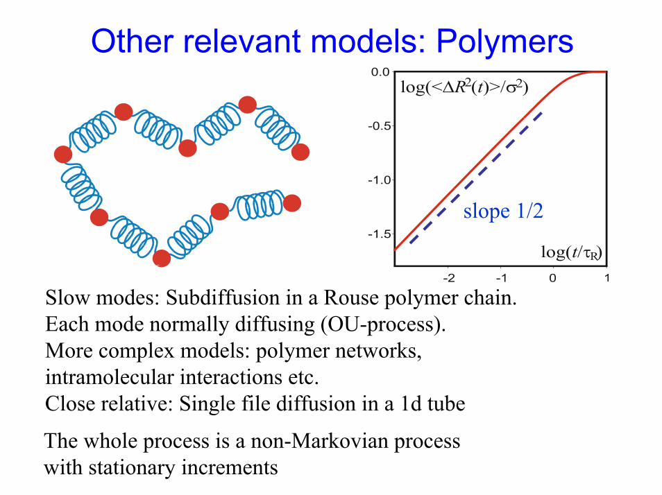
Slow modes: Subdiffusion in a Rouse polymer chain.Each mode normally diffusing (OU-process).More complex models: polymer networks, intramolecular interactions etc. Close relative: Single file diffusion in a 1d tube
Other relevant models: Polymers
The whole process is a non-Markovian process with stationary increments
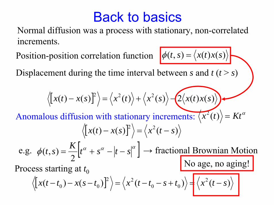
Back to basics
)()(),( sxtxst =φ
[ ] )()(2)()()()( 222 sxtxsxtxsxtx −+=−
Displacement during the time interval between s and t (t > s)
Anomalous diffusion with stationary increments:[ ] )()()( 22 stxsxtx −=−
Process starting at t0
[ ]αααφ ststKst −−+=2
),(
αKttx =)(2
e.g. → fractional Brownian Motion
[ ] )()()()( 200
2200 stxtsttxtsxttx −=+−−=−−−
No age, no aging!
Normal diffusion was a process with stationary, non-correlated increments.Position-position correlation function
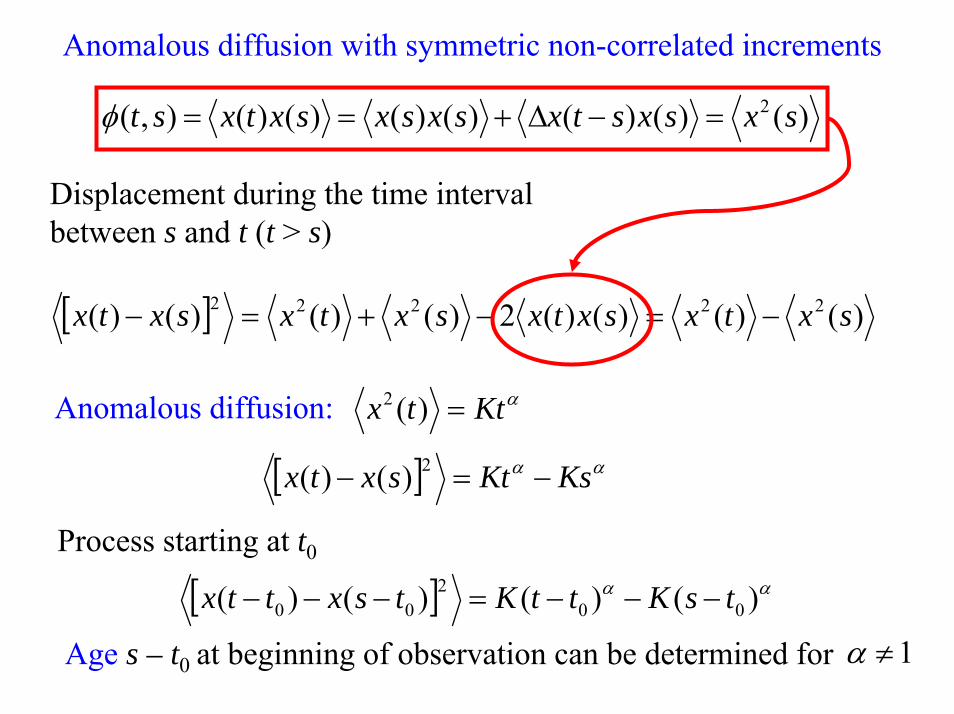
Anomalous diffusion with symmetric non-correlated increments
)()()()()()()(),( 2 sxsxstxsxsxsxtxst =−∆+==φ
[ ] )()()()(2)()()()( 22222 sxtxsxtxsxtxsxtx −=−+=−
Displacement during the time interval between s and t (t > s)
Anomalous diffusion: αKttx =)(2
[ ] αα KsKtsxtx −=− 2)()(
Process starting at t0
[ ] αα )()()()( 002
00 tsKttKtsxttx −−−=−−−
Age s – t0 at beginning of observation can be determined for 1≠α
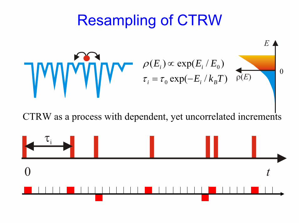
Resampling of CTRW
)/exp()/exp()(
0
0
TkEEEE
Bii
ii
−=∝
ττρ
CTRW as a process with dependent, yet uncorrelated increments
0
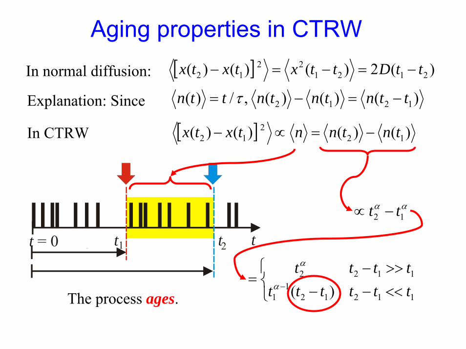
Aging properties in CTRW[ ] )(2)()()( 2121
2212 ttDttxtxtx −=−=−In normal diffusion:
)()()(,/)( 1212 ttntntnttn −=−= τExplanation: Since
t = 0 ttN t1 1 2
The process ages.
[ ] )()()()( 122
12 tntnntxtx −=∝−
⎩⎨⎧
<<−−>>−
=−
112121
1
1122
)( tttttttttt
α
α
αα12 tt −∝
In CTRW
αAttn ≅ens
)(
[ ] [ ]ens1ens2
2
ens
212 )()()()( tntnatxtx −=−
[ ] [ ]∫∫ −+=−+=TT
Tdtttt
TAadttnttn
Tatx
0
2
0ensens
2
ens
2 '')'(')'()'(1)( αα
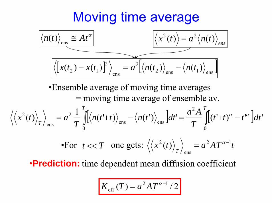
Moving time average
•Ensemble average of moving time averages = moving time average of ensemble av.
enstnatx )()( 22 =
tATatxT
12
ens
2 )( −= αone gets:•For Tt <<
•Prediction: time dependent mean diffusion coefficient
2/)( 12eff
−= αATaTK
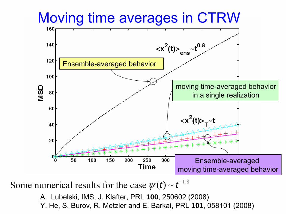
Ensemble-averaged moving time-averaged behavior
Ensemble-averaged behavior
moving time-averaged behaviorin a single realization
Moving time averages in CTRW
8.1~)( −ttψSome numerical results for the caseA. Lubelski, IMS, J. Klafter, PRL 100, 250602 (2008)Y. He, S. Burov, R. Metzler and E. Barkai, PRL 101, 058101 (2008)
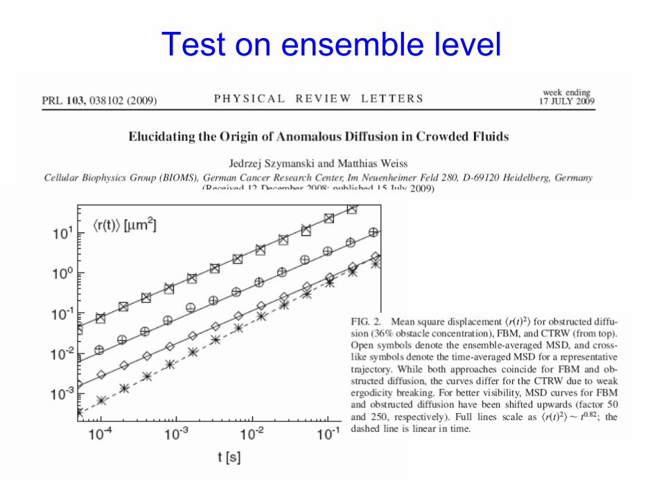
Test on ensemble level
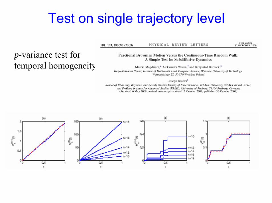
Test on single trajectory level
p-variance test for temporal homogeneity
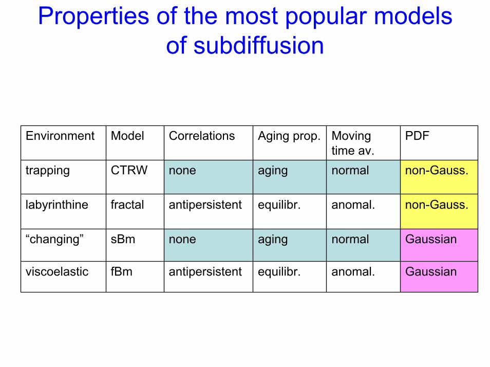
Properties of the most popular models of subdiffusion
Environment Model Correlations Aging prop. Moving time av.
trapping CTRW none aging normal non-Gauss.
labyrinthine fractal antipersistent equilibr. anomal. non-Gauss.
“changing” sBm none aging normal Gaussian
viscoelastic fBm antipersistent equilibr. anomal. Gaussian
• Anomalous is normal
• Happy families are all alike; every unhappy family is unhappy in its own way
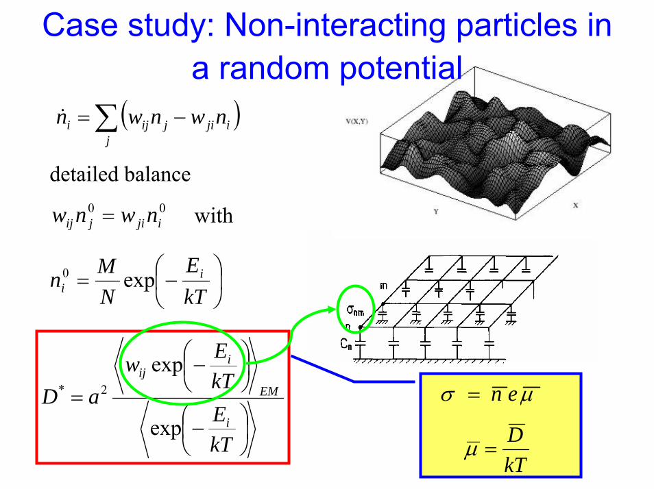
Case study: Non-interacting particles in a random potential
( )∑ −=j
ijijiji nwnwn&
detailed balance00ijijij nwnw = with
⎟⎠⎞
⎜⎝⎛−=
kTE
NMn i
i exp0
⎟⎠⎞
⎜⎝⎛−
⎟⎠⎞
⎜⎝⎛−
=
kTEkTEw
aDi
EM
iij
exp
exp2* µσ en=
kTD
=µ
⎟⎠⎞
⎜⎝⎛−
⎟⎠⎞
⎜⎝⎛−
=
kTEkTEw
aDi
EM
iij
exp
exp2*
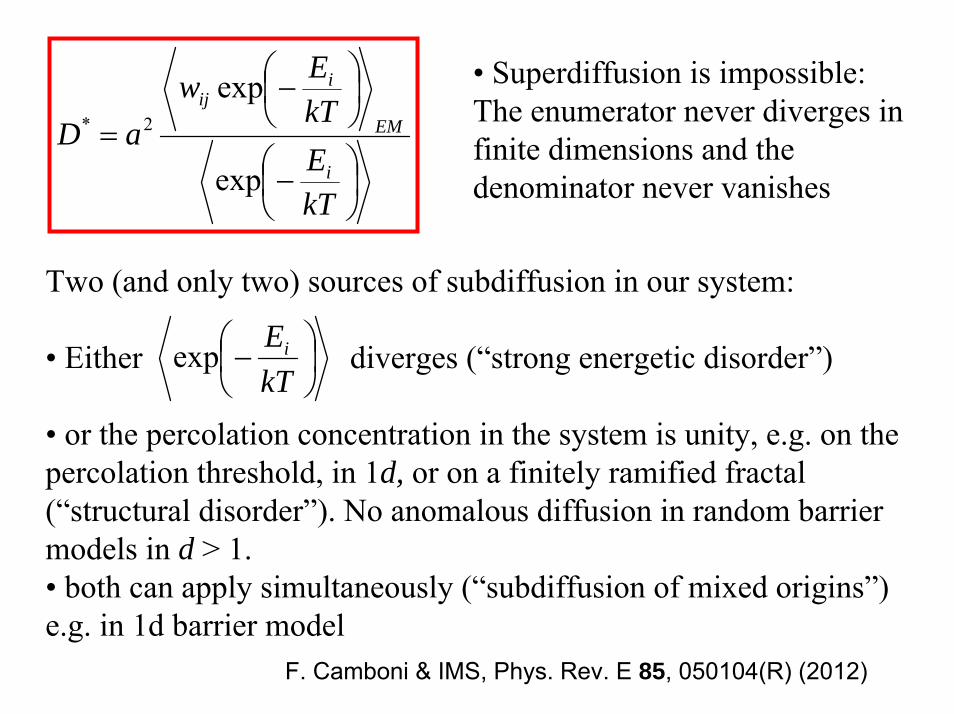
• Superdiffusion is impossible: The enumerator never diverges in finite dimensions and the denominator never vanishes
Two (and only two) sources of subdiffusion in our system:
• Either diverges (“strong energetic disorder”)
• or the percolation concentration in the system is unity, e.g. on the percolation threshold, in 1d, or on a finitely ramified fractal (“structural disorder”). No anomalous diffusion in random barrier models in d > 1.• both can apply simultaneously (“subdiffusion of mixed origins”)e.g. in 1d barrier model
⎟⎠⎞
⎜⎝⎛−
kTEiexp
F. Camboni & IMS, Phys. Rev. E 85, 050104(R) (2012)
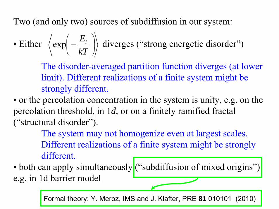
Two (and only two) sources of subdiffusion in our system:
• Either diverges (“strong energetic disorder”)
The disorder-averaged partition function diverges (at lower limit). Different realizations of a finite system might be strongly different.
• or the percolation concentration in the system is unity, e.g. on the percolation threshold, in 1d, or on a finitely ramified fractal (“structural disorder”).
The system may not homogenize even at largest scales. Different realizations of a finite system might be strongly different.
• both can apply simultaneously (“subdiffusion of mixed origins”)e.g. in 1d barrier model
⎟⎠⎞
⎜⎝⎛−
kTEiexp
Formal theory: Y. Meroz, IMS and J. Klafter, PRE 81 010101 (2010)
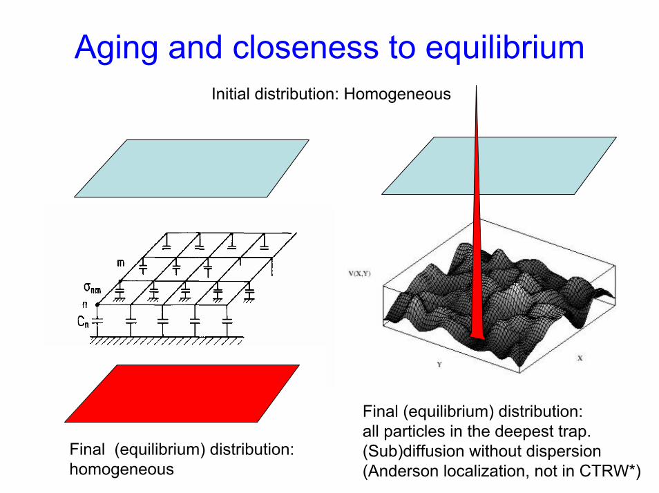
Aging and closeness to equilibriumInitial distribution: Homogeneous
Final (equilibrium) distribution: all particles in the deepest trap.(Sub)diffusion without dispersion(Anderson localization, not in CTRW*)
Final (equilibrium) distribution: homogeneous

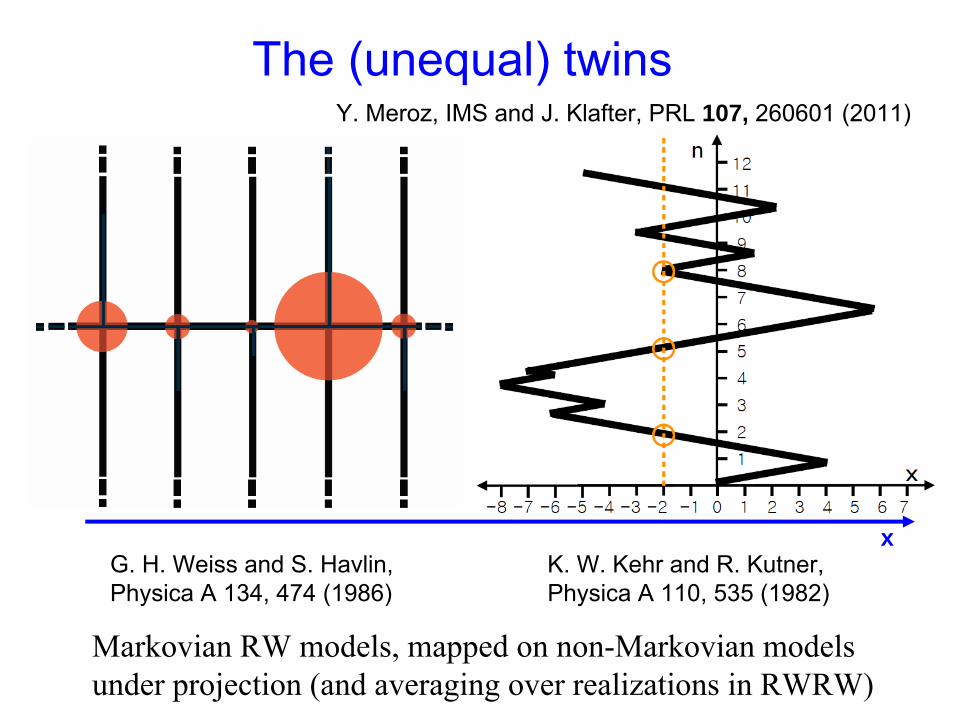
The (unequal) twins
G. H. Weiss and S. Havlin, Physica A 134, 474 (1986)
K. W. Kehr and R. Kutner, Physica A 110, 535 (1982)
x
Y. Meroz, IMS and J. Klafter, PRL 107, 260601 (2011)
Markovian RW models, mapped on non-Markovian models under projection (and averaging over realizations in RWRW)
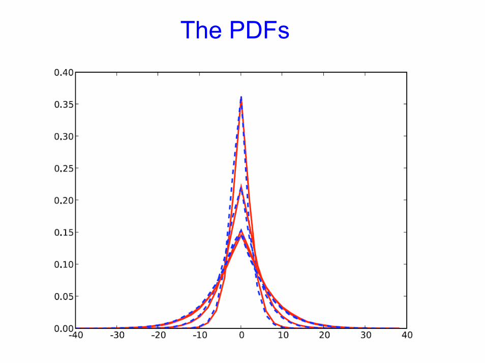
The PDFs
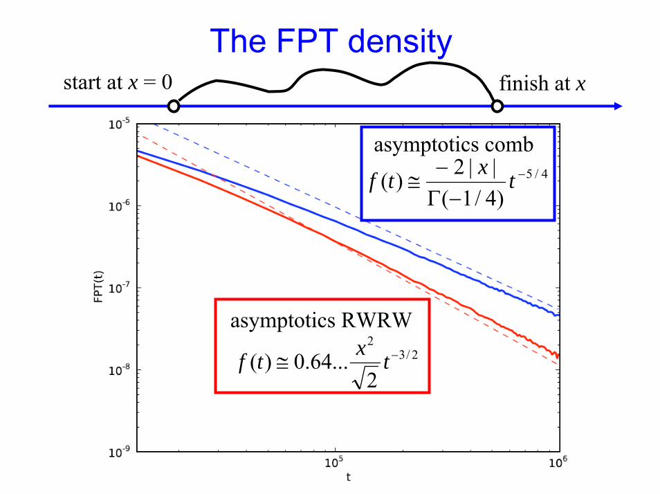
The FPT densitystart at x = 0
4/5
)4/1(||2)( −
−Γ−
≅ txtf
asymptotics comb
2/32
2...64.0)( −≅ txtf
asymptotics RWRW
finish at x

Aging properties
There are three curves here!
ta=0
ta=1000
ta=3000
ta> 0
[ ]22 )()(|)( aat txttxtxa
−+=
stationary
non-stationary
The (unequal) twins
G. H. Weiss and S. Havlin, Physica A 134, 474 (1986)
K. W. Kehr and R. Kutner, Physica A 110, 535 (1982)
x
Y. Meroz, IMS and J. Klafter, PRL 107, 260601 (2011)
Markovian RW models, mapped on non-Markovian models under projection (and averaging over realizations in RWRW)
Take home messages• Anomalous is normal• Happy families are all alike; every unhappy family
is unhappy in its own way• Knowledge of the PDF as a function of time (and
even of an equation for this function) is not too much
• The most important distinction has to be made between models with stationary increments and models with uncorrelated increments.
• Models of mixed origin make the situation even more complex