Univerzita Karlova v PrazeMatematicko-fyzikalnı fakulta

DIPLOMOVA PRACE

Evelina Gabasova

Vstupnı data a jejich vyznam pro vrstevnateneuronove sıte

(Input data and their significance formulti-layered feed-forward neural networks)

Katedra softwaroveho inzenyrstvı

Vedoucı diplomove prace: doc. RNDr. Iveta Mrazova, CSc.,Katedra teoreticke informatiky a matematicke logiky

Studijnı program: Informatika, obor Teoreticka informatika

2010

I would like to

Prohlasuji, ze jsem svou diplomovou praci napsala samostatne a vyhradne s pouzitımcitovanych pramenu. Souhlasım se zapujcovanım prace.

V Praze dne Evelina Gabasova

2

Contents

1 Introduction 6

2 Multi-layered feed-forward neural networks 82.1 Formal neuron . . . . . . . . . . . . . . . . . . . . . . . . . . . . . . . 82.2 Multi-layered feed-forward neural networks . . . . . . . . . . . . . . . 10

3 Training of multi-layered neural networks 133.1 Training of neural networks . . . . . . . . . . . . . . . . . . . . . . . 133.2 Backpropagation algorithm . . . . . . . . . . . . . . . . . . . . . . . . 153.3 Variants of the backpropagation algorithm . . . . . . . . . . . . . . . 173.4 Scaled conjugate gradients . . . . . . . . . . . . . . . . . . . . . . . . 18

4 Techiques to improve generalization 234.1 Generalization and overfitting . . . . . . . . . . . . . . . . . . . . . . 234.2 Regularization . . . . . . . . . . . . . . . . . . . . . . . . . . . . . . . 234.3 Weight decay . . . . . . . . . . . . . . . . . . . . . . . . . . . . . . . 244.4 Early stopping . . . . . . . . . . . . . . . . . . . . . . . . . . . . . . . 244.5 Pruning . . . . . . . . . . . . . . . . . . . . . . . . . . . . . . . . . . 264.6 Enforced internal representation . . . . . . . . . . . . . . . . . . . . . 27

4.6.1 Learning condensed internal representation . . . . . . . . . . . 284.6.2 Learning unambiguous internal representation . . . . . . . . . 30

4.7 Enforced internal representations - mixture of Gaussians . . . . . . . 314.8 Enforced internal representations - minimal entropy . . . . . . . . . . 354.9 Analysis of internal representations produced by the minimal entropy

regularizer . . . . . . . . . . . . . . . . . . . . . . . . . . . . . . . . . 40

5 Experiments 445.1 Toy problem: binary addition . . . . . . . . . . . . . . . . . . . . . . 445.2 Data from the UCI Machine Learning repository . . . . . . . . . . . . 59

5.2.1 Iris Data Set . . . . . . . . . . . . . . . . . . . . . . . . . . . 595.2.2 Contraceptive Method Choice Data Set . . . . . . . . . . . . . 655.2.3 Pima Indians Diabetes Data Set . . . . . . . . . . . . . . . . . 72

5.3 World Development Indicators . . . . . . . . . . . . . . . . . . . . . . 79

3

5.3.1 Preprocessing . . . . . . . . . . . . . . . . . . . . . . . . . . . 795.3.2 Experimental results . . . . . . . . . . . . . . . . . . . . . . . 81

6 Conclusion 89

Bibliography 91

A World development indicators 92

B Countries 99

4

Nazev prace: Vstupnı data a jejich vyznam pro vrstevnate neuronove sıteAutor: Evelina GabasovaKatedra (ustav): Katedra softwaroveho inzenyrstvıVedoucı diplomove prace: doc. RNDr. Iveta Mrazova, CSc.e-mail vedoucıho: Iveta.Mrazova@mff.cuni.cz

Abstrakt: Neuronove sıte stale zustavajı konkurenceschopnym modelem v nekterychoblastech strojoveho ucenı. Jednou z jejich nevyhod je vsak jejich tendence k preucenı,ktera muze vazne omezit jejich schopnost zobecnovat. V predlozene praci studu-jeme ruzne regularizacnı techniky zalozene na vynucovanı internıch reprezentacı vneuronovych sıtıch. Internı reprezentace jsou analyzovany na zaklade noveho teo-retickeho modelu zalozeneho na teorii informace, ze ktereho nasledne vychazı regu-larizator minimalizujıcı entropii internıch reprezentacı. Tento regularizator zalozenyna minimalizaci entropie je vypocetne narocny a z tohoto duvodu je v praci pouzitpredevsım jako teoreticka motivace. Z duvodu potreby efektivnejsı a flexibilnejsıregularizace byl navrhnut novy regularizator zalozeny na Gaussovskem smesovemmodelu aktivacı neuronu. Tento model je srovnan s existujıcımi metodami vynu-covanı internıch reprezentacı v experimentalnı casti prace. Vysledky navrhnutehomodelu jsou lepsı predevsım na klasifikacnıch ulohach.Klıcova slova: regularizace, internı reprezentace, Gaussovsky smesovy model, en-tropie

Title: Input data and their significance for multi-layered feed-forward neural net-worksAuthor: Evelina GabasovaDepartment: Department of Software EngineeringSupervisor: doc. RNDr. Iveta Mrazova, CSc.Supervisor’s e-mail address: Iveta.Mrazova@mff.cuni.cz

Abstract: In the present work we study In some areas, artificial feed forward neuralnetworks are still a competitive machine learning model. Unfortunately they tend tooverfit the training data, which limits their ability to generalize. We study methodsfor regularization based on enforcing internal structure of the network. We analyzeinternal representations using a theoretical model based on information theory. Basedon this study, we propose a regularizer that minimizes the overall entropy of internalrepresentations. The entropy-based regularizer is computationally demanding andwe use it primarily as a theoretical motivation. To develop an efficient and flexibleimplementation, we design a Gaussian mixture model of activations. In the experi-mental part, we compare our model with the existing work based on enforcement ofinternal representations. The presented Gaussian mixture model regularizer yieldsbetter results especially for classification tasks.Keywords: regularization, internal representations, Gaussian mixture model, entropy

5

Chapter 1

Introduction

Artificial feed forward neural networks represent a successful model for statisticalpattern recognition and machine learning. They are widely used in practice and theystand even in competition with some more recent methods, such as the supportvector machines used for classification or Gaussian processes for regression. Somereasons for their success are in the relative simplicity of their use as they do notrequire construction of complex statistical or probabilistic models.

They proved to be effective also on problems with large dimensionality whicharise frequently in many application areas, for example in bioinformatics. A compar-ison study on supervised learning algorithms on high dimensional tasks [?] showedthat neural networks work surprisingly well for such problems as their performanceremains steadily good across many different types of tasks. Other learning algorithmsoften show better performance for some specific types of problems whereas they per-form poor in others. The main advantage of neural networks lies in their universalityand wide applicability.

One of the main problems with learning artificial neural networks lies in theirtendency to overfit to the training data easily. This significantly limits their abilityto generalize. Therefore some generalization technique is usually used to limit net-works’ complexity. Enforced internal representations [24] are one of the successfulregularization schemes. By forcing the hidden units in neural networks to produceonly certain values of activations, neural networks form smoother functions, whichare connected to better generalization capabilities.

The work in this thesis explores the performance of networks with enforced con-densed internal representations on various tasks. It also proposes a new method ofenforcing a particular form of internal representations on hidden units in neuralnetworks, based on Gaussian mixture model. This form of regularizer provides anefficient and flexible method to enforce wide range of different schemes of internalrepresentations.

Another novel algorithm for enforcing internal representations based on the infor-mation theory is proposed in this work. It serves as a theoretical tool for analysis ofinternal representations which are naturally formed in neural networks. This regular-

6

izer minimizes the overall entropy of internal representations formed during trainingof neural networks. This way, it finds the minimal description of the input patternsin terms of the internal representations that preserves the maximum information toapproximate a given target function. The main advantage of entropy is that it doesnot assume any particular form of internal representation. However, the entropy-based regularizer is very computationally demanding and therefore it is proposed toserve as a basic framework which allows analysis of minimal entropy internal rep-resentations. More efficient techniques may be afterwards constructed based on theanalysis. In this work, a Gaussian mixture model of neural activations is constructedusing the information from the minimal entropy configuration.

The experimental part presents a comparison of the algorithm proposed in [24] forenforcing internal representations with the regularizers proposed in this work. Theevaluation of the discussed algorithms is performed both on classification and regres-sion tasks and the formed internal representations are visualised in a novel form withself-organizing maps. This presents a new viewpoint on the formed internal repre-sentations and a platform for assessing the relation between internal representationsand the performance of trained networks.

The rest of this work is organized as follows: Chapter2 gives a brief overview ofthe neural network model which is used in this work. Chapter 3 overviews the opti-mization algorithms which are used to efficiently train neural networks - namely thethe stochastic gradient descent optimization (backpropagation algorithm), gradientdescent with momentum and scaled conjugate gradients. Chapter 4 discusses variousregularization methods used in training neural networks, especially the methods forenforcing internal representations. Chapter 5 presents the evaluation of the gradientdescent algorithm, gradient descent with momentum and scaled conjugate gradientsboth with and without enforced internal representations on several different tasks. Adetailed analysis of the internal representations is also given in this chapter. Finally,Chapter 6 concludes the work with a summary and evaluation of achieved results.

The results presented in this work were implemented in the F# programminglanguage and in Matlab.

7

Chapter 2

Multi-layered feed-forward neuralnetworks

This chapter overviews the basic model of formal neuron and multi-layered artificialneural network which will be used throughout this work.

2.1 Formal neuron

Formal neuron represents the basic processing unit of an artificial neural network.This section gives a brief overview of this concept and its use in the neural networkmodels.

The inspiration for the formal neuron originated from biological neurons. Fol-lowing the natural parallel, the artificial neuron consists of a set of connections(dendrites) which provide the input into the neuron, a body where the activation(excitation) level of the neuron is determined and finally one output connection(axon) which propagates the activation to other neurons. The body computes aweighted sum of its inputs as its so-called potential which is then compared with theneuron’s bias. Finally, the inner potential of the neuron is transformed by a speci-fied activation function (transfer function), which determines the neuron’s activationlevel.

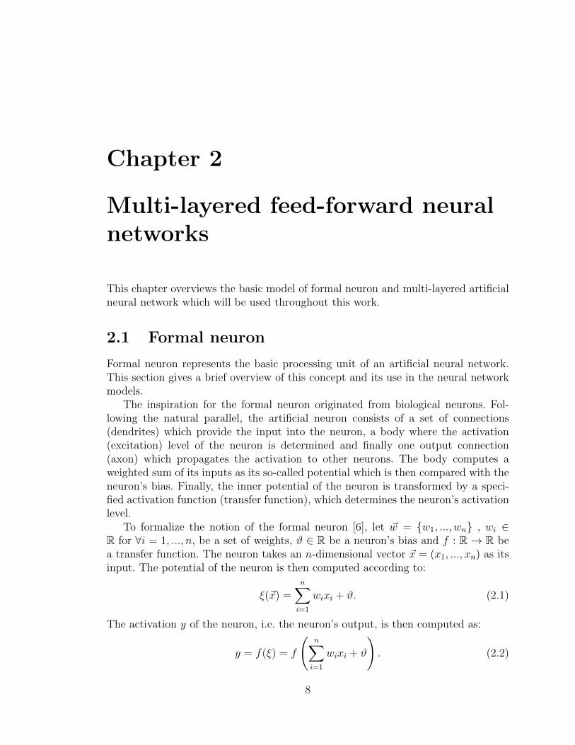
To formalize the notion of the formal neuron [6], let ~w = {w1, ..., wn} , wi ∈R for ∀i = 1, ..., n, be a set of weights, ϑ ∈ R be a neuron’s bias and f : R → R bea transfer function. The neuron takes an n-dimensional vector ~x = (x1, ..., xn) as itsinput. The potential of the neuron is then computed according to:

ξ(~x) =n∑i=1

wixi + ϑ. (2.1)

The activation y of the neuron, i.e. the neuron’s output, is then computed as:

y = f(ξ) = f

(n∑i=1

wixi + ϑ

). (2.2)

8

Figure 2.1: The model of a formal neuron; x1, ..., xn represent the neuron’s inputs,x0 denotes the fictive input for the neuron’s bias w0 = ϑ, x0 = 1, w1, ..., wn are theneuron’s weights, ξ(~x) is the neuron’s potential (Equations 2.1 and 2.2), y is theneuron’s output computed according to Equation 2.3.

for a specified transfer function f . To simplify the notation, the bias ϑ is treated asan extra weight w0 = ϑ from a fictive input x0 = 1, which is formally added to theinput vector. Using this convention, the output of the neuron is computed as

y = f

(n∑i=0

wixi

)(2.3)

where f is the transfer function. This model of a neuron is schematically shown inFigure 2.1.

Various functions are applicable as transfer functions. The use of neurons asadaptive units in multi-layered neural networks with optimization by a gradientdescent-based algorithm sets a condition on the transfer function to be differentiable(as discussed in Chapter 3). Throughout this work, the logistic sigmoid function andthe hyperbolic tangent will be employed as the transfer functions.

The logistic sigmoid f : R→ (0, 1) is defined as:

f(ξ) =1

1 + e−λξ, (2.4)

where λ is the parameter which controls the slope of the sigmoid and ξ is the neuron’spotential (Equation 2.2). If not stated otherwise, λ = 1. This function is shown inFigure 2.2.

The hyperbolic tangent transfer function f : R→ (−1, 1) is defined as:

f(ξ) =eξ − e−ξ

eξ + e−ξ, (2.5)

9

−5 0 5

−1

−0.5

0

0.5

1

ξ

activ

atio

n

Logistic sigmoid

−5 0 5

−1

−0.5

0

0.5

1

ξ

activ

atio

n

Hyperbolic tangent

Figure 2.2: Transfer functions: the logistic sigmoid and hyperbolic tangent

where ξ represents the neuron’s potential (Equation 2.2). This function is againshown in Figure 2.2.

Let us also introduce the classification for states of neurons adopted from [24]. Ifwe consider the logistic sigmoid activation function, a neuron is called active if itsoutput is in the vicinity of 1.0, passive if its activation is close to 0.0 and silent ifthe output is around 0.5. Similarly for the hyperbolic tangent, active state of neuroncorresponds to the output close to 1.0, passive to −1.0 and silent to 0.0.

2.2 Multi-layered feed-forward neural networks

A multi-layered feed-forward neural network (backpropagation network, BP-network)[6] represents a general mapping from a set of input patterns onto a set of outputpatterns. This model gained a great popularity as a versatile non-linear approxima-tor for various tasks. This section gives a brief summary of the general model of aBP-network.

The network consists of individual neurons (Eq. 2.1) organized into layers. Theneurons are connected in such a way, that the connections exists only between neu-rons from different layers. They are also oriented and acyclic in case of the feed-forward neural networks. We shall consider the basic model, where the neurons inconsecutive layers are fully connected. In general some of the connections can beremoved.

The first and last layer are called the input and output layer, respectively. Theother layers between the input and output layers are so-called hidden layers. Thearchitecture of a network is described by numbers of neurons in each of its layers, e.g.2-5-3 is an architecture which corresponds to a network with three layers of neurons,with 2 neurons in the input layer, 5 neurons in the hidden layer and 3 in the outputlayer. The number of neurons in the input layer matches the dimensionality of theinput data.

10

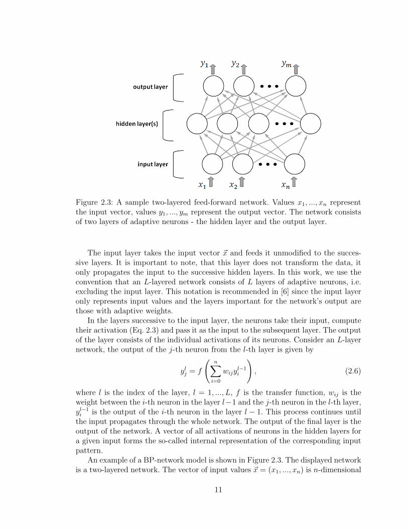
Figure 2.3: A sample two-layered feed-forward network. Values x1, ..., xn representthe input vector, values y1, ..., ym represent the output vector. The network consistsof two layers of adaptive neurons - the hidden layer and the output layer.

The input layer takes the input vector ~x and feeds it unmodified to the succes-sive layers. It is important to note, that this layer does not transform the data, itonly propagates the input to the successive hidden layers. In this work, we use theconvention that an L-layered network consists of L layers of adaptive neurons, i.e.excluding the input layer. This notation is recommended in [6] since the input layeronly represents input values and the layers important for the network’s output arethose with adaptive weights.

In the layers successive to the input layer, the neurons take their input, computetheir activation (Eq. 2.3) and pass it as the input to the subsequent layer. The outputof the layer consists of the individual activations of its neurons. Consider an L-layernetwork, the output of the j-th neuron from the l-th layer is given by

ylj = f

(n∑i=0

wijyl−1i

), (2.6)

where l is the index of the layer, l = 1, ..., L, f is the transfer function, wij is theweight between the i-th neuron in the layer l−1 and the j-th neuron in the l-th layer,yl−1i is the output of the i-th neuron in the layer l − 1. This process continues until

the input propagates through the whole network. The output of the final layer is theoutput of the network. A vector of all activations of neurons in the hidden layers fora given input forms the so-called internal representation of the corresponding inputpattern.

An example of a BP-network model is shown in Figure 2.3. The displayed networkis a two-layered network. The vector of input values ~x = (x1, ..., xn) is n-dimensional

11

and therefore also the input layer has n neurons. The network has a single hiddenlayer. The output layer contains m neurons, which produce the network’s output~y = (y1, ..., ym).

The BP-networks provide a functional mapping from a specified input to anoutput value. Depending on the transfer function, the mapping is usually non-linear.Therefore, they represent a universal powerful tool for function approximation, bothfor classification and regression tasks. The training of BP-networks is discussed inthe following Chapter 3.

12

Chapter 3

Training of multi-layered neuralnetworks

In the previous chapter, the general model of a BP-network was described. In thischapter we continue with a basic overview the basic algorithms to train a network. Inparticular we overview the fundamental backpropagation algorithm and some othergradient descent-based methods.

3.1 Training of neural networks

Machine learning methods can be divided into supervised and unsupervised tech-niques. Unsupervised learning uses only unlabelled data and attempts to organizethem and thus reveal a possible underlying structure in the data. An example of thisapproach is clustering, where the data are partitioned into groups according to somesimilarity criterion. On the other hand, training of a BP-network is an example ofsupervised learning. This method is used to learn a target function which is specifiedby a set of desired outputs.

The training data T consist of a set of pairs

T = {(~xi, ~ti)|~xi ∈ Rn, ~ti ∈ Rm}, (3.1)

where for the i-th training pattern, ~xi is the input vector and ~ti is its desired targetvector.

This training data is used to determine the weights and biases of the networkduring the process of training. The trained network is afterwards used to approximatethe outputs for some input values, for which the target values are unknown.

As has been noted in Section 2.2, BP-networks are used to solve both regressionand classification tasks. In case of a regression problem, networks are used to approx-imate a continuous function. The modelled function then determines the dimensionsof the input and output vectors.

In a classification problem, the task is to sort the inputs into several classes.The classes represent a categorical output, which cannot be directly used as a target

13

function. Therefore, the classes should be encoded in some way. Usually, the binaryor bipolar 1-of-c coding is applied in case of a multi-class task:

ti =

{1 if the input pattern belongs to the i-th class

0 (−1 in case of bipolar coding ) otherwise

(3.2)According to this scheme, the output of a trained network is ~t = (t1, ..., tm) and theinput pattern is classified to a class c according to

c = arg maxi

ti. (3.3)

This allows a classification task to be presented to a BP-network.Neural networks are trained to approximate a given target function by adapting

their weights. This is a task of a multi-variate non-linear optimization. Given theset of training data in the form specified in Eq.3.1, the goal is to find network’sweights that minimize the difference between the desired target values and the actualnetwork’s outputs. The difference is measured by an error function ET (also called theobjective function) on the training set. A frequently used error function is the sum-of-squares error, which measures the squared difference between the actual outputof a network and the demanded target value:

ET =1

2

N∑p=1

m∑j=1

(y(p)j − t

(p)j )2, (3.4)

where ET is the error with respect to the training set, N is the number of trainingpatterns, m is the number of neurons in the output layer, y

(p)j is the activation of the

j-th neuron in the output layer for the p-th training pattern and t(p)j is the desired

target value for the j-th output and p-th training pattern.The task is to minimize the value of the objective function ET . If both the

objective function and the transfer function f 2.3 are differentiable, it is possibleto optimize the parameters of a BP-network by the gradient descent algorithm.The error function is treated as a multivariate function of weights in the network,ET : RW → R, where W is the number of weights and biases in the whole network.The optimization method then attempts to minimize the value of the error functionin the weight space RW .

A general strategy of iterative gradient descent (GD) based algorithms consists ofseveral steps. The optimization in step t starts from a weight vector ~wt (a point in the

weight space). From this point a search direction ~dt is specified with use of the localgradient of the error function at this point. The optimization procedure continuesby selecting a step size, which determines how far to move the weight vector in thechosen direction. The weight vector is updated by moving it in the specified directionby the specified distance. The adaptation step can be written as

~wt+1 = ~wt + α~dt, (3.5)

14

where dt is the search direction determined in the step t and α regulates the stepsize. This process is iterated until the minimum of the objective function is reached.

The crucial steps in this process are choosing the search direction and determiningthe step size. All training algorithms discussed in this work use the described scheme,however they differ in the way they deal with these points in the optimization process.

An interesting result (as discussed in many papers, e.g. [20]) is the so calleduniversal approximation property of BP-networks. A two-layer network with a sig-moidal transfer function is capable of approximating every continuous function to anarbitrary accuracy. However, this is a theoretical result and the important practicalissue lies in training of such networks, which is discussed in the following sections.

3.2 Backpropagation algorithm

Gradient descent method forms the base of the backpropagation (BP) algorithm [?],which is described below. In the algorithm, the BP-network is first presented withan input pattern, which is propagated forward through the network. The error iscomputed in the final layer of the network and it is propagated backwards to thefirst hidden layer while the weights in the network are adapted to new values. It usesthe gradient descent (steepest descent) method of optimizing the parameters of aBP-network.

A formal description of the backpropagation algorithm is provided for the sum-of-squares error function (Eq. 3.4). For simplicity, we omit the index of the trainingpattern p and the index of the network’s layers l in the algorithm description. Theindex j will correspond to neurons in the currently processed layer, the indexes i andk will correspond to the preceding layer and the successive layer respectively.

To minimize the error function in time step t, each weight wij is adjusted in thedirection opposite to the gradient in the weight space, the derivative of the trainingerror function ET with respect to this weight is computed using the chain rule:

−∂ET∂wij

= −∂ET∂yj· dyjdξj· ∂ξj∂wij

. (3.6)

This term represents the direction, in which the weights are adjusted. The derivativesare evaluated for both the output layer and hidden layers according to:

−∂ET∂wij

= δjyi (3.7)

where (3.8)

δj =

{(tj − yj)dyjdξj

for the neuron j in an output layerdyjdξj

∑k δkwjk for the neuron j in a hidden layer

(3.9)

The termdyjdξj

depends on the activation function which is used:

15

Logistic sigmoiddyjdξj

= yj(1− yj)

Hyperbolic tangentdyjdξj

= 1− y2j

The derivative of the error function is used to adapt the weights in the network:

wij(t+ 1) = wij(t) + α∂ET∂wij

= wij(t) + αGDδjyi, (3.10)

where αGD is the learning rate for the gradient descent algorithm. The learning ratedetermines the size of the step, which is taken in the direction of negative gradient.

Algorithm 1 gives a schematic description of the backpropagation algorithm.

Algorithm 1 The backpropagation algorithm

1: Randomly initialize weights in the network.2: Present a pattern (~x,~t), ~x = (x1, ..., xn), ~t = (t1, ..., tm) to the network, compute

the activations of neurons in the network in the forward pass and compute itsoutput ~y = (y1, ..., ym) for this pattern

3: Compute the value of the objective function ET according to Eq. 3.44: Adapt the weights according to the following rules (3.9):

wij(t+ 1) = wij(t) + αGDδjyi

δj =

{(tj − yj)dyjdξj

for a neuron in an output layerdyjdξj

∑k δkwjk for a neuron in a hidden layer

where wij(t) is the weight between the neurons i and j in the step t and αGD > 0is the learning rate.

5: If a specified stopping criterion is met, stop training, otherwise go to step 2.

The weights and biases of a BP-network are initialized to random values in thebeginning of the training process. Then the training proceeds in epochs, duringone epoch the whole set of training patterns is presented in successive steps to thenetwork. The process is repeated until some specified stopping criterion is met. Theformulation of the backpropagation algorithm (Alg. 1) is a case of stochastic gradientdescent (on-line gradient descent), where the weights are adapted after presentationof each training pattern. Batch (off-line) gradient descent adapts the weights onlyafter all training patterns (or their subset) are presented. In case of batch gradientdescent, there is a larger risk of overtraining than it is for the stochastic variant [?].

In the ideal case, the training should be stopped when the global minimum ofthe error function is reached. However in practice, it is difficult to reach such a pointbecause of highly non-linear nature of the error function. Therefore there exists a widechoice of possible stopping criterions. For example, the training can be stopped whenthe error of the network on the set of training patterns decreased to some predefined

16

Gradient descent

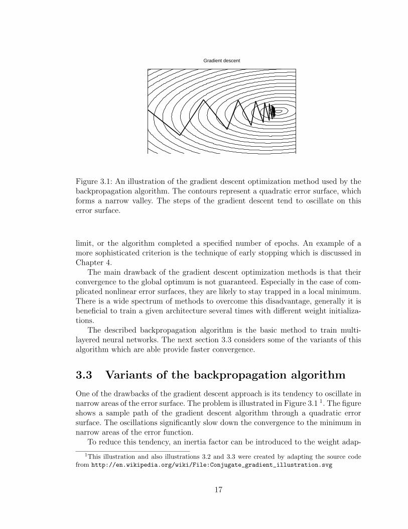
Figure 3.1: An illustration of the gradient descent optimization method used by thebackpropagation algorithm. The contours represent a quadratic error surface, whichforms a narrow valley. The steps of the gradient descent tend to oscillate on thiserror surface.

limit, or the algorithm completed a specified number of epochs. An example of amore sophisticated criterion is the technique of early stopping which is discussed inChapter 4.

The main drawback of the gradient descent optimization methods is that theirconvergence to the global optimum is not guaranteed. Especially in the case of com-plicated nonlinear error surfaces, they are likely to stay trapped in a local minimum.There is a wide spectrum of methods to overcome this disadvantage, generally it isbeneficial to train a given architecture several times with different weight initializa-tions.

The described backpropagation algorithm is the basic method to train multi-layered neural networks. The next section 3.3 considers some of the variants of thisalgorithm which are able provide faster convergence.

3.3 Variants of the backpropagation algorithm

One of the drawbacks of the gradient descent approach is its tendency to oscillate innarrow areas of the error surface. The problem is illustrated in Figure 3.1 1. The figureshows a sample path of the gradient descent algorithm through a quadratic errorsurface. The oscillations significantly slow down the convergence to the minimum innarrow areas of the error function.

To reduce this tendency, an inertia factor can be introduced to the weight adap-

1This illustration and also illustrations 3.2 and 3.3 were created by adapting the source codefrom http://en.wikipedia.org/wiki/File:Conjugate_gradient_illustration.svg

17

Gradient descent with momentum

Figure 3.2: An illustration of the gradient descent optimization method with mo-mentum. The contours represent a quadratic error surface, which forms a narrowvalley. The oscillations of the steps of the backpropagation algorithm are smoothedout and the algorithm converges faster to the minimum.

tation procedure 3.9. Adding a momentum term partly smooths out the oscillations.When the weights are adapted, the momentum term takes previous search directions(previous values of weights) into account:

wij(t+ 1) = wij(t) + αGDδjyi + αMom(wij(t)− wij(t− 1)). (3.11)

In the above formula, (t − 1), (t), (t + 1) represent the successive steps during thetraining process, wij(t) represents a weight between neurons i and j in the step (t)and αMom stands for the momentum rate, 0 ≤ αMom ≤ 1.

The momentum rate αMom is a parameter which value has to be chosen exper-imentally with respect to the actual dataset. It might be difficult to determine itsoptimal value. Larger values of this parameter may lead to even more oscillationsduring the learning process. On the other hand, smaller values may increase a chanceto end in a sub-optimal local minimum. However, when the value of αMom is chosencarefully, it speeds up the convergence. An illustration of improved performance ofthe gradient descent algorithm when the momentum term is introduced is given inFigure 3.2.

3.4 Scaled conjugate gradients

The conjugate gradient (CG) method [?] is a general optimization method for solvingsparse systems of linear equations based on the gradient descent principle. In contextof neural networks, it converges significantly faster than the simple steepest descentalgorithm because of use of second order information and different choice of thesearch direction (Section 3.1).

18

The aim of selecting a more sophisticated choice of the search direction is toprevent oscillations in the weight space during the optimization. The gradient descentmethod often takes steps in directions similar to previously taken steps, even inthe case of a quadratic error function with unique minimum (see Figure 3.1). Theconjugate gradient algorithm solves this problem by selecting directions that areso-called mutually conjugate.

We say that two vectors ~x and ~y are conjugate with respect to a square matrixA (or A-orthogonal) if the following condition holds:

~xTA~y = 0. (3.12)

In our optimization task, we require the successive search directions d0, ...dk to beconjugate with respect to the Hessian matrix H = E ′′(~w):

~diTH~dj = 0; i 6= j; i, j = 0, 1, .., k (3.13)

A detailed reasoning can be found for example in [?] or [6].It is possible to determine these successive search directions iteratively during

the learning process. At the initial weight point, the direction ~d0 is set equal to thenegative gradient ~g0 = −E ′T ( ~w0). Successive directions ~dt, t = 1, ..., k are chosen to

be conjugate with all previous search directions ~ds, s = 0, ..., s − 1. Schematically,the conjugate directions are computed according to:

~dt+1 = ~gt+1 + βt~dt, (3.14)

where ~gt+1 is the value of the negative gradient in step t+1, ~dt is the previous searchdirection and βt is a parameter. The values of βt are determined by applying theconjugacy condition (3.13) on dt+1 and dt:

βt =~gt+1

THdtdTt Hdt

. (3.15)

Since the formula for βt requires computationally demanding calculation of Hessian,approximations are used in practice - common approximation formulas are Hestenes-Stiefel [?], Polak-Ribiere [?] or Fletcher-Reeves [?].

By the requirement of mutual conjugacy of the search directions dt, previouslyperformed steps are not partially annulated, as in the case of simple gradient descent(Figure 3.1). The algorithm is guaranteed to find the minimum of a quadratic errorfunction in at most W steps, where W is the dimension of the error space [?]. Fora detailed analysis, see for example [6], [?]. An illustration of this process is givenin Figure 3.3. There, the quadratic error surface is 2-dimensional and the algorithmfinds the minimum in two steps.

The algorithm in its original form did not deal with nonlinear objective functions.In its application on such tasks, the directions gradually lose their conjugacy and

19

Conjugate gradients

Figure 3.3: An illustration of the conjugate gradient optimization method. The con-tours represent a 2-dimensional quadratic error surface. ForW -dimensional quadraticerror functions, the algorithm converges in at most W steps. In this case, it finds theminimum of the error function in two steps.

therefore the algorithm must be restarted at least every W -th iteration [?]. In therestart, the search direction is simply reset to the current local negative gradient.

Choosing the search direction is only the first important aspect of the algorithm.Apart from this, the step size for time step t αt (from 3.5) must be determined toupdate weights in the specified direction. An exact formula for αt can be derivedhowever it is not used for nonlinear problems as it again involves costly computationof the full Hessian matrix. Instead, the conjugate gradients algorithm computes thestep size usually by some line search technique. Such methods search along theselected direction for a (local) minimum based on some approximation of the errorfunction. This method is less demanding than the computation of the Hessian as itcorresponds to a search for minimum in only one selected dimension in the weightspace. However, it usually requires several evaluations of the objective function, whichstill makes this process very time consuming [22].

The scaled conjugate gradients algorithm (SCG) [22] does not perform the linesearch, instead it uses a simple and efficient approximation of the Hessian (step 2 inAlgorithm 2). The approximation is possible due to the fact that the Hessian figuresin the formulas for αt and βt only in the form of a product with dt.

Another issue in nonlinear optimization with conjugate gradients is a require-ment on the Hessian to be positive definite. This condition holds for quadratic errorfunctions but rarely for nonlinear objective functions. This often prevents the al-gorithm from finding any local minima of the error function. The SCG algorithmuses a standard optimization method of model trust region (an approach used inthe Levenberg-Marquardt algorithm, [6]) to compensate for the indefiniteness of theHessian. For this purpose, an additional adaptive parameter λj (step 4 is introduced.

20

However, the indefiniteness is regulated only locally and therefore the model can betrusted only in the local region of the current point.

The full SCG algorithm is stated in Algorithm 2.

Algorithm 2 Scaled conjugate gradients

1: Choose weight vector ~w(0) and scalars σ, λ0, λ0 such that0 < σ ≤ 10−4, 0 < λ0 ≤ 10−4, λ0 = 0.

Set ~d0 = ~g0 = −E ′( ~w(0)) and t = 0; success = true.2: If success = true, then calculate second order information:

σt = σ

‖~dt‖,

~st = E′(~w(t)+σt ~dt)−E′(~w(t))σt

,

δt = ~dTt ~st.3: Scale δt : δt = δt + (λt − λt)‖dt‖2.4: If δt ≤ 0 then make the Hessian matrix positive definite:

λt = 2(λt − δt‖dt‖2 ),

δt = −δt + λt‖dt‖2,λt = λt.

5: Calculate step size: αt =~dt

T~gt

δt.

6: Calculate the comparison parameter: ∆t = 2δt(E(~w(t)−E(~w(t)+α~dt))

(~dtT~gt)2

.

7: If ∆t ≥ 0 then a successful reduction in error can be made:~w(t+ 1) = ~w(t) + αt~dt,~gt+1 = −E ′(~wt+1),λt = 0, success = true.If t mod W = 0 then restart algorithm: ~dt+1 = ~gt+1,

else βt =‖~gt+1‖2−~gTt+1~gt

~dtT~gt

,

~dt+1 = ~gt+1 + βt~dt.If ∆t ≥ 0.75 then reduce the scale parameter:λt = 1

4λt,

else λt = λt,success = false.

8: If ∆t < 0.25 then increase the scale parameter:λt = λt + δt(1−∆t)

‖~dt‖2.

9: If the steepest descent direction ~gt 6= ~0,then increment t = t+ 1 and go to 2,

else terminate and return ~w(t+ 1) as the minimum.

Among the main variables used in the algorithm, ~w(t) is the weight vector in thetime step t, λt compensates for the indefiniteness of the Hessian matrix H, dt is thesearch vector in time t, gt is the negative gradient in time t. Detailed description of thealgorithm can be found in [22]. The results indicate that this algorithm converges

21

significantly faster than the backpropagation algorithm and than the traditionalconjugate gradients [22].

22

Chapter 4

Techiques to improvegeneralization

4.1 Generalization and overfitting

The goal in training BP-networks is to capture important underlying features, whichare crucial for correct regression/classification of the data. A well trained networkis able to process previously unseen or noisy patterns correctly, i.e. it is able togeneralize the information acquired from the training data set.

One of the main factors that hinder the capability to generalize is noise whichis present in the training data. BP-networks tend to learn the exact image of thethe input-target mapping, including the noise. Therefore, their error on previouslyunseen data deteriorates and their error on such data is significantly larger than theerror on the training set. The networks, which are not able to generalize well fromthe training patterns, are called overfitted.

The problem of overfitting frequently arises when the network is unnecessarillycomplex and has excess capacity which allows it to fit also the noise in the data.The overfitted mapping provided by such a network is often characterized by highcurvature. Another factor that contributes to overfitting is limited amount of data.In such situation, it is particularly hard for the network to identify the underlyingmapping from the noise and capture important features.

There exists a wide variaty of techniques to deal with overfitting and enhancegeneralization ability of BP-networks, some of which are discussed in the followingsections.

4.2 Regularization

Regularization is a general approach to control and limit the complexity of a BP-network. Regularization techniques allow a complex model to be trained on a limitedamount of data with smaller risk of overfitting [6]. Most of these techniques force the

23

network to form smoother mappings by adding a penalty term to the error function:

E = ET + αRER, (4.1)

where ET is the error on the training set 3.4 αT , ER is the complexity penalizationterm and αR is a parameter, which regulates the extend of the effect of the penaltyterm. A large value of αR would lead to over-smoothing of the network’s mappingand poor performance. On the other hand, small values minimize the smoothingeffect and allow high curvature mappings to form. The merit of this method dependson an appropriate choice of this parameter.

The additional term ER may have many forms, but it is mostly constructedto penalize models with higher curvature, as they are frequently connected withdeteriorated performance in generalization [6]. The augmented objective function Ethen favours smooth functions to form during training.

4.3 Weight decay

Weight decay [6] is a simple regularization method which penalizes high curvaturesof network’s mapping. This problem is often associated with relatively large weightsin the network which cause excessively high variance in the output of the network[?].

The weight decay term, which is added to the standard error function 3.4, penal-izes large weights:

1

2

∑i

w2i , (4.2)

where i runs over all weights and biases of the network. The sum of squared weightsand biases is added to the error function and thus penalizes large weights, unlessthey are strongly supported by the data.

The value of the modified objective function is computed by the following formula(based on ??):

EWD = ET + αWD

(1

2

∑i

w2i

), (4.3)

where ET is a standard error function of the network (Eq. 3.4), αWD the a parameterwhich regulates the importance of the weight decay term. As a result, the weights aredriven to zero if they are not crucial for the performance of a BP-network. However,the quality of results strongly depends upon good choice of the coefficient αWD.

4.4 Early stopping

Another widely used form of regularization is the technique of early stopping. Thismethod effectively controls complexity of the network by stopping the training pro-cess at some point before the network overfits.

24

epochs

erro

r

trainingvalidation

Figure 4.1: Error curves for the training set and the test set during a training session(idealized model). The training should be stopped in the point of the minimum ofthe validation error.

During training of a BP-network, the error of the whole network with respect toa training set typically decreases. However, at some point in the training process, thenetwork starts to overfit to the training data. To prevent the overfitting, an additionalsubset of the data is used as the so-called validation set which is disjoint with theoriginal training data set. The validation set acts as an independent measure of thequality of training and simulates the perfomance of the network on a previouslyunseen data. Therefore, the validation set should be representative with respect topossible input data.

During a typical training session, the error on the training set decreases gradually.However, the error with respect to the validation set decreases up to some point whereit starts to increase as the network overfits. The basic intuition says that the trainingshould be stopped in the point of the minimum of the validation error to preventoverfitting in the following epochs of training. An illustration of this process is givenin Figure 4.1.

In real-world situations, the validation error typically does not have only a singleminimum, but several different local minima before the point where the networkstarts to severely overfit [26]. Therefore the optimal stopping point must be deter-mined in some heuristic fashion. An empirical evaluation of various early stoppingcriteria is given in [26] and [?].

The early stopping criterion used in this work is based on the recommendationin [26] for the situations when the aim is to maximize average quality of solutionswhen the networks have tendency to overfit. This criterion uses the notion of trainingstrips which are sequences of consecutive epochs during training of a specified length(usually five epochs). The validation error is measured only at the end of each strip.

25

The training is stopped if the validation error increased in s consecutive strips. Thisis a strong indication of more serious overfitting. In the end, the best performingnetwork is returned as the solution.

4.5 Pruning

When training a neural network on a specific task, it is necessary to set the archi-tecture of the network sufficiently large to capture the complexity of the task. Onthe other hand the architecture is desired to be small because the networks withlimited complexity do not overfit easily. To approximate an optimal architecture isnot an easy task and also the training of such architectures can be more difficultthan training of larger networks with extra free capacity.

Pruning is a method which restricts the architecture of an already trained net-work. This technique removes redundant neurons which are not essential for thenetwork’s performance. Usually, redundant neurons do not contribute enough to theoutput of the network and therefore may be eliminated without changing the overallmapping produced by the network.

Some techniques concern only removal of individual redundant weights. For ex-ample, the weight decay penalization (Section 4.3) drives the weights towards zeroduring training, unless they are supported by the data. After training, the weightsclose to zero can be removed without altering the output of the network signifi-cantly. Therefore training with weight decay can be viewed as a form of pruning. Inthe following text, only the pruning techniques which operate with removal of wholeneurons will be discussed.

A pruning method proposed by Sietsma and Dow [27] discriminates between twotypes of non-contributing neurons. The fist type of neuron produces approximatelyconstant activation for all input patterns in the training set. The second type ofneuron produces similar outputs as some other neuron in the same layer. Both typesof neurons can be removed without the risk of changing the output of the trainednetwork. We will briefly overview the methods to remove the described types ofneurons. Detailed reasoning is given in [27].

A neuron with approximately constant activation across all training patterns ef-fectively serves only as an additional bias for neurons in the successive layer. There-fore, it is possible to incorporate the constant activation of this neuron as an ad-ditional bias to already present biases of neurons in the next layer, which receiveoutputs of the redundant neuron.

Consider a neuron i which has approximately the same output across the wholetraining set. Let yi be the average activation of this neuron. To remove this neuron,we have to adapt biases ϑj of neurons j which receive the outputs from the deletedneuron according to the following equation:

ϑ′j = ϑj + wij yi, (4.4)

26

where wij is the weight between neurons i and j. The output of neuron i is there-fore redistributed and the overall output of the network remains approximately un-changed.

The second type of neuron mimics activations of some other neuron from the samelayer. First let us consider two neurons i and k which produce approximately identicalactivations across the whole training set, i. e. yi ≈ yk for all training patterns. Oneof these neurons can be removed provided that the weights of the remaining neuronare doubled to preserve output of the whole network. Consider removal of the neuroni. The altered weights between the neuron k (which is to remain) and neurons j inthe successive layer are then given by:

w′kj = wkj + wij, (4.5)

where wkj is the original weight between neurons k and j and wij is the originalweight between the discarded neuron i and j.

Another similar case is when two neurons i and k always produce exactly oppositeoutputs, i. e. for the logistic sigmoid as activation function: yi ≈ 1−yk, yi, yk ∈ (0, 1).It is again possible to remove one of these neurons, e. g. neuron i, by applying thefollowing:

ϑ′j = ϑj + wij (4.6)

w′kj = wkj − wij. (4.7)

The index j again signifies the index of a neuron in the consecutive layer, ϑj repre-sents its bias, wij is the weight between the discarded neuroon i and neuron j andfinally wkj is the weight of the remaining neuron k.

By pruning a BP-network using the described technique, the output should stayapproximately unchanged. The crucial point in this approach is identifying the neu-rons which may be discarded without deterioration of performance. A transpar-ent internal representation (Section 2.2) may be beneficial in selecting such non-contributing neurons. The following sections consider some variants of enforcingtransparent internal representations on BP-networks which encourage a network toform transparent structure and simplify the identification of redundant neurons.

4.6 Enforced internal representation

As has been noted in the previous section, it is beneficial when BP-networks formtransparent internal representation (Section 2.2). It represents an advantage not onlyfor pruning of such networks but also for the generalization. Standard BP-networksmay form internal representations which are non-transparent and scattered over thewhole interval of possible activations. Therefore it is difficult to determine significanceof individual hidden neurons to the overall network’s output. Also the network maybecome trained to use only small differences in activations to discriminate between

27

some patterns which leads to deteriorated generalization. The method of enforcedinternal representation proposed in [24], [25], forces the network to form a transparentinternal representation during training.

Transparent internal representations are enforced using the regularization tech-nique by introducing an additional penalization parameter to the error function(Eq:4.1). Let us first introduce some definitions. An internal representation is calledcondensed, if the hidden neuron’s activations are grouped around the values 0, 0.5and 1 for sigmoid transfer function, or −1, 0 and 1 for the hyperbolic tangent. Thesevalues correspond respectively to so-called passive, silent and active states of a neu-ron. When a BP-network generates condensed internal representations, it’s internalstructure is transparent and significance of roles of individual neurons is easier todetermine. Therefore, it can be successfully used to prune the network.

Another advantageous property for a BP-network is when the internal representa-tions are as different as possible for significantly different outputs. Such requirementprevents networks to distinguish patterns with different targets only by some smallchange in activations. Otherwise only a small change in the input pattern may causea significant change in the output. Internal representations which pass this require-ment are called unambiguous.

The method of enforced internal representations [?] aims to force a BP-network toform both condensed and unambiguous internal representations. These requirementsare incorporated into the learning process by including an additional terms in theobjective function used to train a network. The penalty terms are discussed in moredetail in the following two sections.

4.6.1 Learning condensed internal representation

Training of BP-networks while enforcing condensed internal representation is per-formed according to a standard regularization technique of an additional term in theobjective function. In this case, the term should force activations of hidden neuronsto group around their passive, silent and active states. The values of states differ fordifferent transfer functions, for the logistic sigmoid passive state corresponds to theactivation 0, silent to 0.5 and active to 1; for the hyperbolic tangent the values are−1, 0 and 1 respectively.

The method presented in [24] uses a polynomial penalty term which has minimain the desired values of activations. For a given single activation y the regularizationterm takes the following form:

ECIR(y) = (1− y)sys(y − 0.5)2, (4.8)

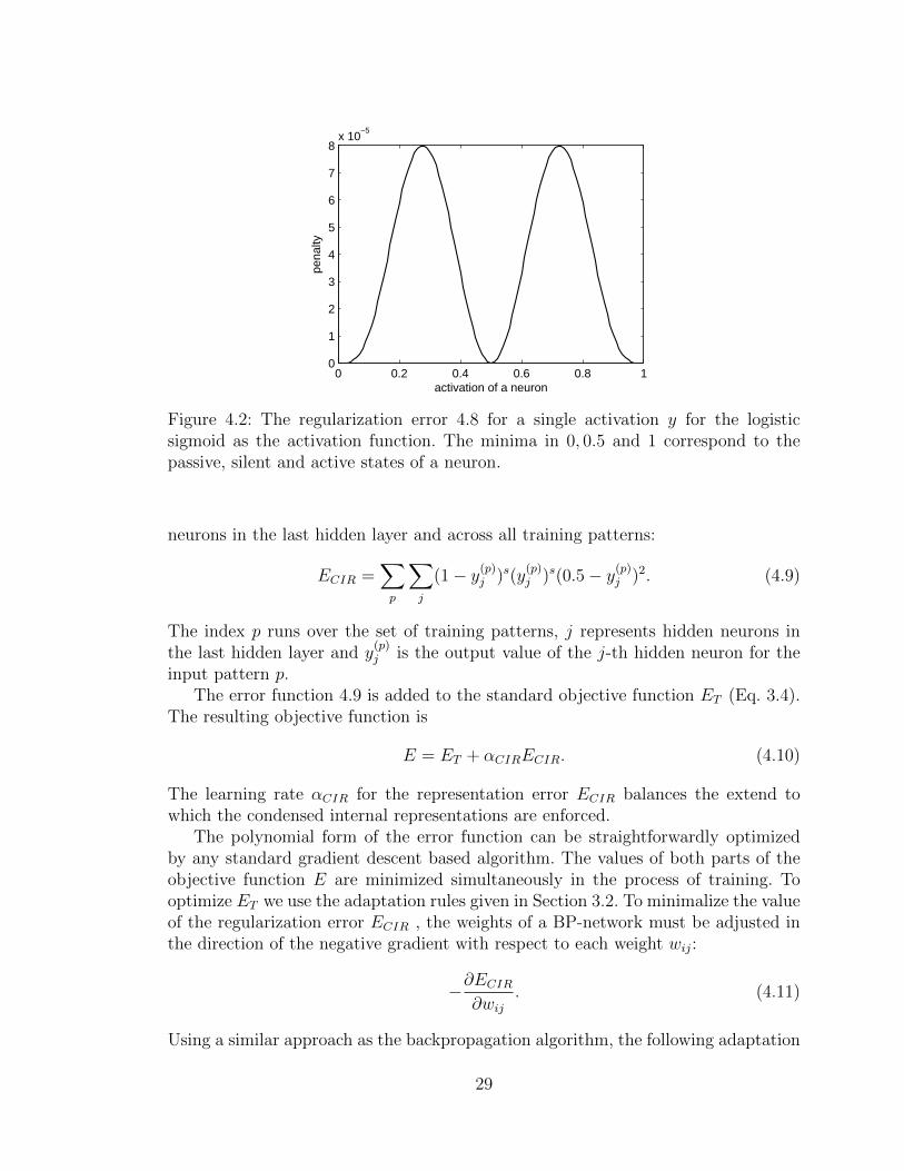
where the exponent s > 1. The value of s recommended in [24] is s = 4. Figure 4.2displays the plot of this regularization term for a single activation y.

The full objective function for logistic sigmoid transfer function for enforcingcondensed internal representations is the sum of the individual errors 4.8 across all

28

0 0.2 0.4 0.6 0.8 10

1

2

3

4

5

6

7

8x 10

−5

activation of a neuron

pena

lty

Figure 4.2: The regularization error 4.8 for a single activation y for the logisticsigmoid as the activation function. The minima in 0, 0.5 and 1 correspond to thepassive, silent and active states of a neuron.

neurons in the last hidden layer and across all training patterns:

ECIR =∑p

∑j

(1− y(p)j )s(y

(p)j )s(0.5− y(p)

j )2. (4.9)

The index p runs over the set of training patterns, j represents hidden neurons inthe last hidden layer and y

(p)j is the output value of the j-th hidden neuron for the

input pattern p.The error function 4.9 is added to the standard objective function ET (Eq. 3.4).

The resulting objective function is

E = ET + αCIRECIR. (4.10)

The learning rate αCIR for the representation error ECIR balances the extend towhich the condensed internal representations are enforced.

The polynomial form of the error function can be straightforwardly optimizedby any standard gradient descent based algorithm. The values of both parts of theobjective function E are minimized simultaneously in the process of training. Tooptimize ET we use the adaptation rules given in Section 3.2. To minimalize the valueof the regularization error ECIR , the weights of a BP-network must be adjusted inthe direction of the negative gradient with respect to each weight wij:

−∂ECIR∂wij

. (4.11)

Using a similar approach as the backpropagation algorithm, the following adaptation

29

rules are derived (a detailed reasoning can be found in [24]):

wij(t+ 1) = wij(t) + αGDδjyi + αCIR%jyi (4.12)

where

%j =

0 for output neurons

−[2(s+ 1)yj(1− yj)− s2]ysj (1− ysj )(yj − 0.5)

for neurons from the last hidden layer

yj(1− yj)∑

k ρkwjk for other neurons

(4.13)

where wij(t) is the weight between neurons i and j in the step t, yi and yj areoutputs of neurons i and j respectively, δj is defined the same way as in the standardbackpropagation algorithm (Equation 3.9), αGD > 0 is the learning rate from thebackpropagation algorithm. In addition, αCIR > 0 is the learning rate for the internalrepresentation error.

The adaptation rules apply to a BP-network with the logistic sigmoid transferfunction. The rules for the hyperbolic tangent can be derived by adapting the valuesof passive, silent and active states and by incorporating the corresponding derivativeof the transfer function.

4.6.2 Learning unambiguous internal representation

Unambiguous internal representations are enforced in a similar manner as the con-densed internal representations. In this case, the cost function is designed to favourinternal representations which differ from each other as much as possible for verydifferent target patterns [24]. In other words, it only punishes a network for creatingsimilar internal representations when the desired outputs are different.

In [24], the objective function EUIR for enforcing unambiguous internal represen-tations is constructed to yield large negative values when large differences betweentarget values are bounded with dissimilar internal representations. For distinct tar-gets accompanied with similar internal representations, EUIR would yield values closeto 0. It has to be noted, that different internal representations connected with similartarget values should not be penalized, because they may contribute to the network’sability to learn the task.

Function EUIR as proposed in [24] has the following form:

EUIR = −1

2

∑p

∑q 6=p

∑j

∑o

(t(p)o − t(q)o )2(y(p)j − y

(q)j )2, (4.14)

where the indices p and q represent training patterns, j is an index of individualneurons in the last hidden layer and the index o runs over neurons in an outputlayer. Variable y represents actual output of a neuron for a given training patternand t is the desired target value for the particular pattern.

30

The objective function EUIR is added to the network’s general objective functionas a regularizer (Eq. 4.1). Both the condensed and unambiguous internal represen-tations can also be enforced simultaneously:

E = ET + αCIRECIR + αUIREUIR, (4.15)

where the parameters αCIR and αUIR regulate the trade-off between individual ob-jective functions, ET is the standard training error function for backpropagation(Eq. 3.4), ECIR and EUIR are the errors for condensed and unambiguous internalrepresentations.

Similarly as for the condensed internal representations, the unambiguous repre-sentations are enforced using a gradient descent approach. Each weight wij in thenetwork is moved in the direction opposite to the local gradient:

−∂EUIR∂wij

. (4.16)

This leads to the following adaptation rules, as derived and presented in [24]:

wij(t+ 1) = wij(t) + αGDδjyi + αCIR%jyi + αUIRτjyi (4.17)

where

τj =

0 for output neurons∑

q 6=p Tq(yj − y(q)j )yj(1− yj) for neurons from the last hidden layer

yj(1− yj)∑

k τkwjk for other neurons

(4.18)

where Tq =∑o

(t(p)o − t(q)o )2. (4.19)

where p is the actually processed training pattern and other parameters are thesame as in Equation 4.13. To maintain consistent notation with previously statedadaptation rules, the index of the pattern p was omitted.

The time and space complexity of the whole training task increases with addingthe above stated unambiguous term. To evaluate contribution of this term to theadaptation rules, it is necessary to go through the whole training set for each of thetraining patterns. Especially for large training sets, this can increase the complexitysignificantly. This algorithm is not included in the experimental part of this work.

4.7 Enforced internal representations - mixture of

Gaussians

Another method of enforcing condensed internal representation proposed in this workuses a probabilistic mixture model for the internal representations. In our case, we

31

−1 −0.5 0 0.5 10

0.2

0.4

0.6

0.8

1

1.2

1.4

1.6

1.8

σ2 = 0.01

σ2 = 0.03

σ2 = 0.05

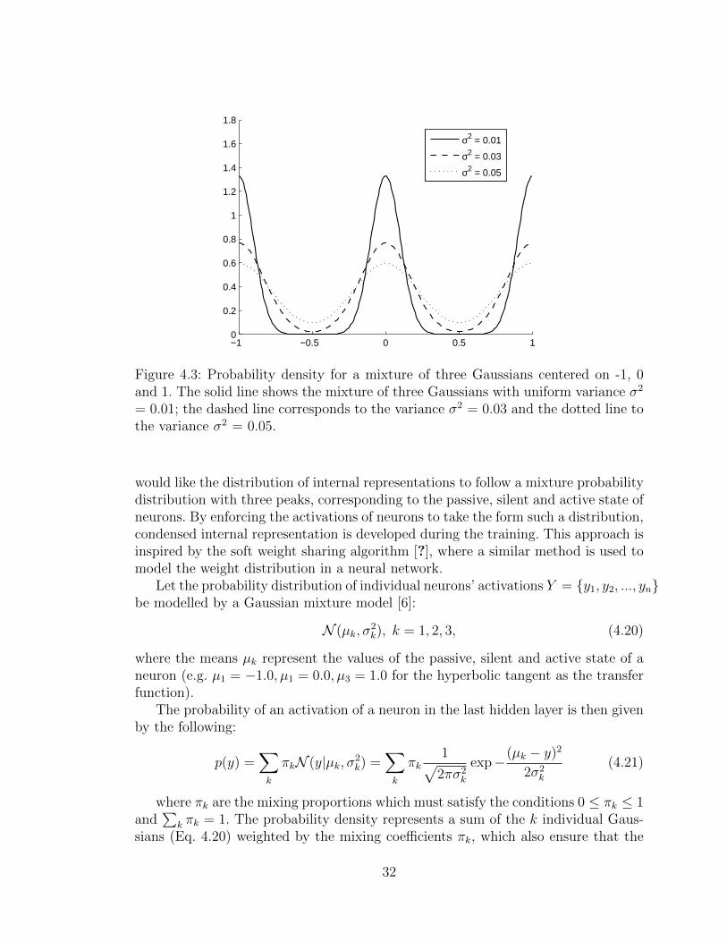
Figure 4.3: Probability density for a mixture of three Gaussians centered on -1, 0and 1. The solid line shows the mixture of three Gaussians with uniform variance σ2

= 0.01; the dashed line corresponds to the variance σ2 = 0.03 and the dotted line tothe variance σ2 = 0.05.

would like the distribution of internal representations to follow a mixture probabilitydistribution with three peaks, corresponding to the passive, silent and active state ofneurons. By enforcing the activations of neurons to take the form such a distribution,condensed internal representation is developed during the training. This approach isinspired by the soft weight sharing algorithm [?], where a similar method is used tomodel the weight distribution in a neural network.

Let the probability distribution of individual neurons’ activations Y = {y1, y2, ..., yn}be modelled by a Gaussian mixture model [6]:

N (µk, σ2k), k = 1, 2, 3, (4.20)

where the means µk represent the values of the passive, silent and active state of aneuron (e.g. µ1 = −1.0, µ1 = 0.0, µ3 = 1.0 for the hyperbolic tangent as the transferfunction).

The probability of an activation of a neuron in the last hidden layer is then givenby the following:

p(y) =∑k

πkN (y|µk, σ2k) =

∑k

πk1√

2πσ2k

exp−(µk − y)2

2σ2k

(4.21)

where πk are the mixing proportions which must satisfy the conditions 0 ≤ πk ≤ 1and

∑k πk = 1. The probability density represents a sum of the k individual Gaus-

sians (Eq. 4.20) weighted by the mixing coefficients πk, which also ensure that the

32

−1 −0.8 −0.6 −0.4 −0.2 0 0.2 0.4 0.6 0.8 1−2

0

2

4

6

8

10

12

14

σ2 = 0.01

σ2 = 0.03

σ2 = 0.05

Figure 4.4: Cost functions for a mixture of three Gaussians centered on -1, 0 and 1.The solid line corresponds the mixture of three Gaussians with uniform variance σ2

= 0.01; the dashed line corresponds to the variance σ2 = 0.03 and the dotted line tothe variance σ2 = 0.05.

result is a valid probability density. Examples of a Gaussian mixture models for neu-ron activations are shown in Figure 4.3, they represent models for condensed internalrepresentations for the hyperbolic tangent transfer function, i.e. for the activationsgrouped around the values −1, 0 and 1. The figure displays three different densities,each with uniform variance σ2 = 0.01, 0.03 and 0.05 respectively.

To enforce the presented probability model 4.21 on the activations of hiddenneurons, we specify the following objective function EGM , which is added to thestandard error function ET :

EGM = −∑j

ln

(∑k

πkpk(yj)

), (4.22)

where j runs over neurons in the last hidden layer. The objective function is definedas the weighted sum of probabilities of an activation to belong to a specific componentof the mixture model. The terms are transformed by the natural logarithm for easiermanipulation of the exponential in the Gaussians.

Figure 4.4 shows the plot of the cost functions corresponding to the probabilitydistributions in Figure 4.3. Compare this plot with Figure 4.2 which shows the costfunction for polynomial-enforced internal representations.

To optimize the cost function 4.22 via a gradient method, the derivative of thecost function with respect to the individual weights in the BP-network is computed

33

as follows:∂EGM∂wij

= −

(∑k

rk(yj)µk − yjσ2k

)∂yj∂wij

(4.23)

where

rk(yj) =πkpk(yj)∑l πlpl(yj)

(4.24)

and

pk(yj) =1√

2πσ2k

exp−(µk − yj)2

2σ2k

. (4.25)

In the above equations, wij is the weight between neurons i and j in a neural net-work, yj is the activation of the j-th neuron and pk(yj) is the probability of a givenactivation yj under the k-th Gaussian. The term rk(yj) is interpreted the respon-sibility of the k-th Gaussian in the mixture for explaining the activation yj in thecontext of Gaussian mixture models [6].

The general adaptation rules for weights in a BP-network has the following form:

wij(t+ 1) = wij(t) + αGDδjyi + αGMγjyi (4.26)

where

γj =

0 for the output layerdyjdξj

∑k

rk(yj)µk − yjσ2k

for the last hidden layer

dyjdξj

∑l

γlwjl for other hidden layers

(4.27)

The term αGM is the learning rate for the Gaussian mixture model regularizer andthe derivative

dyjdξj

depends on transfer function.

Gaussian mixture models have the advantage of increased flexibility in terms ofthe shape of the objective function. It is possible to define a mixture model withnon-uniform variances (heteroscedastic model), where each of the Gaussian has dif-ferent variance. This way the internal representations may be controlled in a moreadvanced way. Figure 4.5a shows the probability density of a mixture model, wherethe Gaussians centered on -1 and 1 have variances 0.1, the Gaussian centered on0 has variance 0.3. Figure ?? shows the corresponding objective function for thismixture with non-uniform variances. This objective function enforces bipolar inter-nal representations (activations -1 and 1) while allowing the activations to take thevalues in between occasionally.

34

−1 −0.5 0 0.5 10.2

0.25

0.3

0.35

0.4

0.45

0.5

(a) Gaussian mixture density

−1 −0.5 0 0.5 10.7

0.8

0.9

1

1.1

1.2

1.3

1.4

1.5

(b) Objective function

Figure 4.5: Probability density and cost function for a mixture of three Gaussianscentered on -1, 0 and 1 with non-uniform variances σ2

1 = σ23 = 0.1, σ2

2 = 0.3.

4.8 Enforced internal representations - minimal

entropy

The two methods of enforcing internal representations described in Sections 4.6 and4.7 both operate with some predefined values of activations, which form the con-densed internal representation. The method which proposed in this section does notuse any fixed set of values for activations. Instead, the method uses the informationtheory approach to minimize the entropy [?] of internal representations which areformed during training.

This method follows the approach of general information bottleneck technique[?], which is used to find the best trade-off between accuracy and complexity ofa model. It finds the minimal description of the input patterns in terms of theinternal representations that preserves the maximum information to still predict thetarget. The main advantage of entropy is that it does not assume any particular formof internal representation. Therefore the minimal-entropy configuration of internalrepresentations can show what form is optimal for the neural network to both fit thedata and regularize the complexity of the network.

To optimize the entropy of internal representations by gradient descent-basedalgorithm, a general method of constructing differentiable estimate of entropy from[?] was used. The following sections give a brief overview of this method, details andderivation of the presented results can be found in [?] and [?].

Differentiable estimate of probability density The entropy of a randomvariable is defined using probability density, therefore it is necessary to first get adifferentiable estimate of the density. For this purpose, the kernel density estimation(Parzen window, [?]) provides a nonparametric smooth and differentiable solution.

35

Let Y be a random variable representing vectors of internal representations. LetT = {~y(1), ~y(2), ...~y(n)} be a sample from this random variable, i.e. a set of internalrepresentations for the set of inputs {~x(1), ~x(2), ...~x(n)}. Then the empirical kernelestimate of the probability density p(~y) for a given internal representation ~y is givenby

p(~y) =1

|T |∑~y(p)∈T

K(~y − ~y(p)), (4.28)

where K is the kernel function and ~y(p) is the internal representation which corre-sponds to the p-th input pattern ~x(p). The density estimate represents the averageof kernel functions centered on each of the internal representations from the randomsample T . The multivariate Gaussian kernel is used as the kernel function:

K(~z) = N (~0,Σ) =1

(2π)d2 |Σ| 12

exp(−1

2~zTΣ−1~z), (4.29)

where Σ is the covariance matrix and d is the dimensionality of ~z.The covariance matrix Σ acts as a form of regularizer for the density estimate.

When the covariances (kernel widths) between internal representations are large,the estimate is excessively smoothed and does not model the data. On the otherhand, when the covariances have very small values, the estimate overly depends onindividual data points and forms series of narrow bumps, each centered on a singleinternal representation.

Therefore it is necessary to choose the values of Σ carefully. It is possible tooptimize the kernel widths automatically by maximum likelihood (ML). We willoptimize the empirical log-likelihood:

L = ln∏~y(p)∈S

p(~y(p)) =∑~y(p)∈S

ln∑~y(q)∈T

K(~y(p) − ~y(q))− |S| ln |T |. (4.30)

In this equation, S is a sample from the random variable Y independent of thefirst sample T . The second sample is introduced because the maximum likelihoodestimation is constructed to make the sample S most likely under the density p(~y)estimated from the sample T .

The maximum likelihood estimate can be distorted by quantization of the datasamples by limited floating point precision. For example, when the data values aregiven with three significant digits, they fall into bins of width b = 0.001 (they arequantized into the bins). To compensate for this quantization, a quantization noiseis added to 4.29 and the kernel function takes the following form:

K(~z) =1

(2π)d2 |Σ| 12

exp(−1

2(~zTΣ−1~z + κ(~bTΣ−1~b)), (4.31)

where ~b are the quantization bin widths and κ is a constant. In [?], κ is set to1/6.

36

Another problem with the maximum likelihood kernel is the need of an indepen-dent sample of the internal representations S apart from the sample T . The suggestedapproach in [?] for the situation with limited amount data available is to for each~y(p) ∈ S use T = S\{~y(p). This approach is similar to that used in the leave-one-outcross-validation.

To maximize the likelihood and get the maximum likelihood kernel, a gradientascent method is used in [?]. For computational reasons, the situation is restricted to

diagonal covariance matrices, which can be represented by a vector ~σ: Σ = diag( ~σ2),σk will denote the k-th element in this vector, i.e. k-th kernel width. The gradientof the likelihood with respect to the covariances is

∂L

∂σk=∑~y(p)∈S

∑~y(q)∈T

((y

(p)k − y

(q)k )2 + κb2

k

σ3k

− 1

σk

)πpq, (4.32)

where

πpq =K(~y(p) − ~y(q))∑

~y(r)∈T K(~y(p) − ~y(r)). (4.33)

The values πpq represent a proximity measure which shows, how the vectors of inter-nal representations ~y(p) and ~y(q) are close to each other given the distances betweenall other internal representations in the sample T .

The covariances are optimized in the log-space, where it is easier to reach steadyconvergence because of the shape of the log-likelihood (detailed reasoning is given in[?]):

ln~σ(t+ 1) = ln~σ(t) + η∂L

∂ ln~σ, (4.34)

where ~σ(t) is the covariance vector in the time step t and η is the learning rate.Exponentiation of this equation leads to the exponentiated gradient learning rule[?]:

~σ(t+ 1) = ~σ(t) · exp(η~g(t) · ~σ(t)). (4.35)

In this equation, ~g(t) denotes the gradient of the likelihood function for the ~σ eval-uated in the step t:

~g(t) =∂L

∂~σ

∣∣∣~σ(t)

. (4.36)

Fro numerical and computational reasons, an approximation of the exponential isused exp(x) ≈ max(1

2, 1 + x). This gives us the following adaptation rule:

~σ(t+ 1) = ~σ(t) ·max[1

2, 1 + η~g(t) · ~σ(t)]. (4.37)

In [?], the general learning rate η is replaced by individual learning rates ηk foreach element of the covariance vector (kernel width) σk to speed up the convergence

37

of the maximum likelihood estimate. These learning rates are adapted independentlyfor each kernel width using the adaptation rule:

ηk(t+ 1) =

{ψηk(t) if gk(t)gk(t− 1) > 0

ηk(t)/ψ otherwise.(4.38)

The parameter ψ is set to 1.5 according to [?].The previous reasoning applied to the situation where all the kernels have the

same variance (homoscedastic kernels). However, individual shapes of kernels mayapproximate the probability density more accurately, especially in situations withdiscontinuities. The given equations can be generalized to this heteroscedastic modelby having a separate covariance matrix Σp for each individual kernel function Kp

centered on the p-th internal representation y(p).After this modification, the kernel density estimate 4.28 takes the following form:

p(~y) =1

|T |∑~y(p)∈T

Kp(~y − ~y(p)). (4.39)

The proximity measure πpq (Equation 4.33) is modified accordingly:

πpq =Kq(~y(p) − ~y(q))∑

~y(r)∈T Kr(~y(p) − ~y(r))

. (4.40)

Also the learning rates ηp are individually adjusted for each kernel function Kp

and the gradient ~gp for the p-th kernel is modified from 4.32 to the following:

∂L

∂σqk=∑~y(p)∈S

((y

(p)k − y

(q)k )2 + κb2

k

(σqk)3

− 1

σqk

)πpq. (4.41)

This forms the nonparametric density estimation with maximum likelihood kernelshapes that is fully differentiable.

Optimizing the entropy by gradient descent The derived estimation ofprobability density is used to optimize the estimate of the entropy of a set of internalrepresentations in a BP-network. The entropy [?] of a continuous random variableY is defined as:

H(Y ) = −∫p(~y) ln p(~y)d~y. (4.42)

This theoretical entropy is then approximated from the available empirical sampleof internal representations S = {y(1), y(2), ..., y(|S|)} from the random variable Y :

H(Y ) = − 1

|S|∑~y(p)∈S

ln p( ~y(p)) = − 1

|S|∑~y(p)∈S

ln∑~y(q)∈T

Kj(~y(p) − ~y(q)) + ln |T |. (4.43)

38

The entropy estimate acts as the cost function for the neural network. To optimizethe cost function by the means of gradient descent, the derivative of this functionwith respect to the set of weights ~w in the network is computed as follows:

∂

∂ ~wH(Y ) =

1

|S|∑~y(p)∈S

∑~y(q)∈T

πpq

(∂~y(p)

∂ ~w− ∂~y(q)

∂ ~w

)(Σq)−1(~y(p) − ~y(q)), (4.44)

where πpq is the proximity measure defined in 4.40. It is important to note, thatthe set of weights ~w consists of the weights, which lead to hidden layers that formthe internal representations. It does not include the weights between the last hiddenlayer and the output layer.

This gradient of the entropy estimate is used in optimization of the objectivefunction for the neurons in the hidden layers, that constitute the internal represen-tation. The optimization process follows the general technique (Eq.4.1) of includingan additional objective function to the standard error function ET (Eq.3.4) . Theadaptation rule for weight updates of these neurons takes the following form:

wij(t+ 1) = wij(t) + αGDδjyi + αEεij (4.45)

where εij =∑~y(q)∈T

πpq

(∂y

(p)j

∂wij−∂y

(q)j

∂wij

)· 1

(σ2j )q· (y(p)

j − y(q)j ) (4.46)

=∑~y(q)∈T

πpq

(dy

(p)j

dξ(p)j

y(p)i −

dy(q)j

dξ(q)j

y(q)i

)· 1

(σ2j )q· (y(p)

j − y(q)j ) (4.47)

where p is the index of the pattern, that is processed at the moment, αGD and δjare defined the same way as in Algorithm 1, αE is the learning rate for the entropyregularizer; wij is the weight from neuron i to neuron j, y

(p)j is the activation of

the j-th neuron after presenting the p-th input pattern x(p) to the neural network;(σ2

j )q is the j-th element of the variance vector (kernel width) of the kernel function

corresponding to the q-th internal representation y(q); ξ(p)j is defined in 2.3 as the

weighted sum of the inputs into the neuron j, the derivative dy(p)j /dξ

(p)j depends on

the transfer function that is used in the network.To give a summary, the general adaptation rule for weights in the BP-network

39

with entropy-enforced internal representation is

wij(t+ 1) = wij(t) + αδjyi + αEεij (4.48)

where

εij =

0 for neurons in the output layer∑~y(q)∈T πpq

(dy

(p)j

dξ(p)j

y(p)i −

dy(q)j

dξ(q)j

y(q)i

)· 1

(σ2j )q · (y

(p)j − y

(q)j )

for neurons in the last hidden layer

dy(p)j

dξ(p)j

y(p)i

∑k

εjkwjk for other hidden layers

(4.49)

The term αE is the learning rate for the entropy-based regularizer. Simultaneouslywith the weights, the kernel covariances for each of the training patterns are alsoadapted according to the exponentiated gradient adaptation rule 4.37.

4.9 Analysis of internal representations produced

by the minimal entropy regularizer

The method of enforcing minimal-entropy configuration on the internal representa-tions is more computationally demanding than the other two discussed methods. Itrequires a pass through the whole data set for every iteration and also the compu-tation of gradient for adaptation of kernel covariances. It is very computationallydemanding to use this method on larger data sets. Therefore, this method was in-tended more as a theoretical tool to analyse the internal representations which arenaturally formed in a neural network. Both the previously presented regularizers forenforcing internal representations work with some predefined desired values of ac-tivations and enforce these values during training. The minimal entropy regularizerpresents a way to explore the naturally formed internal representations, which maybe afterwards used as a basis for the other regularizers.

An experimental training was performed on some of the data sets from the UCImachine learning repository, which are described in detail in the following Chapter5. Here, an analysis of minimal-entropy internal representations is presented for thewell-known iris data set, which is also introduced in more detail in Section 5.2.1.Briefly, the data set consists of four measurements of sepal and petal width andlength for three species of the iris plant - iris setosa, iris virginica and iris versicolor.The whole data set contains 150 patterns, each species of the iris flower is representedby 50 patterns. The goal of this task is to predict the class label (iris setosa, irisvirginica or iris versicolor) based on the four measured attribute values.

BP-networks with the architecture 4 - 5 - 3 with logistic sigmoid transfer functionwere trained on this task in 10-fold cross-validation. The networks were trained bygradient descent GD with enforced minimal-entropy internal representations GD-E

40

Table 4.1: Training results for the minimal-entropy regularizer on the iris data setfor the gradient descent optimization algorithm.

AlgorithmRegularizerlearningrate

Training: MSE Training:Correct (%) Test:Correct (%)

GD 0.026 ± 0.012 98.7 ± 0.7 96.0 ± 3.4GD-E 0.1 0.250 ± 0.031 81.3 ± 4.1 86.0 ± 9.1GD-E 0.01 0.260 ± 0.059 81.0 ± 6.0 83.3 ± 10.1GD-E 1.0e-6 0.239 ± 0.043 84.9 ± 5.0 82.0 ± 10.9GD-E 1.0e-10 0.058 ± 0.018 96.8 ± 1.3 94.7 ± 5.3

for various values of the entropy learning rate αE, each for 500 epochs which wasenough for the networks to converge. The value of the learning rate for gradientdescent was experimentally set to αGD = 0.08. It was difficult to balance the rate ofenforcing internal representations with learning the task. Therefore, the average per-formance of the regularizer was mostly worse than the performance of the standardgradient descent algorithm. Nevertheless, the results provide an interesting insightinto the naturally formed internal representations.

Some of the training results are presented in Table 4.1. The values of the meansquared error on the training and test sets and the percentage of correctly learnedpatterns is compared. The standard gradient GD descent yielded the best results. Toexplain the results, the formed internal representations were analysed in more detail.

Figure 4.6 shows the internal representations formed in one of the networkstrained by gradient descent, which reached 100 % correctness on the test set. Therows represent vectors of individual internal representations and and the activationlevel is presented on greyscale. The colours that surround the vectors signify theclass of the corresponding input. As we can see, the internal representations for irissetosa are very similar to each other and well condensed. The other two classes ofthe iris plant have less differentiate internal representations.

The internal representations formed with enforced minimal entropy for two ofthe values of entropy learning rate are displayed in Figure 4.7. The lower value ofαE (Figure 4.7a) produced a not very condensed representation, as a lot of unitshave their activation somewhere on the greyscale. However, the activation patternsshow lower entropy compared to the internal representations produced by standardgradient descent, as they approximately follow a simple pattern for each of the classes.

The next figure 4.7b shows the internal representations of a network trained withenforced minimal entropy with αE = 0.1. Now the representation is perfectly bipolar,all the hidden neurons are either fully active or fully passive for every input pattern.This is also the reason of worse performance of the networks trained with enforcedminimal entropy - the networks soon became too rigid to fit the data well.

41

passive silent active

Activations

Iris setosa

Iris versicolor

Iris virginica

Figure 4.6: Internal representations formed in a BP-network with 4 - 5 - 3 topologytrained by gradient descent GD on the iris data set. White color represents activeneurons (with activation 1), black color corresponds to silent networks (activation0), other values of activations are displayed on greyscale. The colours that surroundeach internal representation specify the class of the corresponding input.

Figure 4.8 shows a histrogram of activations from Figure 4.7a. The most of theactivations are grouped around the passive (0) and active (1) states. In between, thedistribution of activations is approximately uniform. Similar results were achievedalso with other networks trained in the same way. This result forms the foundation ofthe Gaussian mixture model regularizer with non-uniform variances, which is illus-trated in Figure 4.5. This regularizer mimics the distribution of activations producedby the minimal-entropy regularizer, such that the activations are encouraged to beeither fully active or fully passive but they are not penalized for not being silent(activation equal to 0.5). The objective function is almost constant for the values inthe middle of the interval of possible activations.

The performance of Gaussian mixture regularizer with non-uniform variances iscompared to the performance of the other discussed algorithms for enforcing con-densed internal representations in the following chapter.

42

passive silent active

Activations

Iris setosa

Iris versicolor

Iris virginica

(a) αE = 1.0e-10 (b) αE= 0.1

Figure 4.7: Internal representations formed in a BP-network with 4 - 5 - 3 topologytrained by gradient descent with enforced minimal-entropy internal representationsGD-E on the iris data set. White color represents active neurons (with activation 1),black color corresponds to silent networks (activation 0), other values of activationsare displayed on greyscale. The colours that surround each internal representationspecify the class of the corresponding input.

0 0.2 0.4 0.6 0.8 10

50

100

150

200

250

300

350

activation

Figure 4.8: Histrogram of values of activations for a BP-network trained by gradientdescent with enforced minimal-entropy internal representations, αE = 1.0e-10

43

Chapter 5

Experiments

5.1 Toy problem: binary addition

The first set of experiments deals with training BP-networks on addition of binarynumbers. The presented algorithms on enforcing internal representations were usedto train BP-networks and their performance was evaluated with respect to noisy datato asses generalization capabilities of the trained networks.

The task of binary addition is an artificially designed problem. The training setof patterns consists of combinations of two 4-bit binary numbers, the sum of thetwo numbers represents the desired target. Therefore, the inputs are binary vectorsof total length 8 and the targets are binary vectors of length 5. The training set isformed by all 256 possible patterns. The inputs and targets from the training setare displayed in Figure 5.1 and Figure 5.2. The figures display the input and targetvectors in a visual form as vectors of squares, where the black squares represent 0and the white squares represent 1. As an illustration, number of carry bits neededto compute the sum of two binary numbers in input vectors is displayed by a colournext to each vector.

The discussed algorithms were tested on a set of 100 networks with weights ran-domly initialized from the interval [-1.0, 1.0]. All networks used the logistic sigmoidas their transfer functions. Several topologies were tested with 8 to 20 hidden units.The results are presented for the topologies with 8 and 10 hidden neurons, as they areable to reveal the most about the nature of the task and illustrate the performanceof each algorithm.

The tested algorithms are listed in Table 5.1. The following notation is used: αGDis the learning rate for gradient descent (backpropagation), αMom is the momentumrate and Variances represent the variances of individual components in the Gaussianmixture model (Section 4.7). The abbreviations which are given in the table will beused through the whole experimental chapter.

For the standard backpropagation algorithm (GD, stochastic gradient descentoptimization), the value of the learning rate αGD was experimentally optimized;starting from αGD = 1.0, the value was repeatedly reduced by a factor of 10 and

44

Number of carry bits

0

1

2

3

4

Figure 5.1: Inputs for the task of binary addition. The input patterns are binary vec-tors of length 8 and represent two 4-bit numbers. The binary values are representedby black (0) and white (1) squares. The colours that surround each vector representthe number of carry bits needed during the computation of the binary sum of twonumbers.

trained networks were compared. The value of αGD for the binary addition taskwas set to the value corresponding to the best performing networks, αGD = 0.1.The same procedure was performed to optimize the momentum rate αMom, the bestperformance was achieved for αMom = 0.1. Learning rates for the regularizers werealso tested in a similar way, however the results of the regularized networks are shownfor several of the parameters to better asses their capabilities and their sensitivity tothe values of their parameters. The values of these learning rates are specified in theindividual tables with training results. Among the tested algorithms, the gradientdescent, gradient descent with momentum and scaled conjugate gradients were usedas the baseline for evaluation of the performance of each of the regularizers.

The networks were trained using the whole data set until sufficient performancewas reached - mean squared error (MSE) less or equal to 0.01, or until a maximalnumber of epochs was reached. The maximum was set to 5000 epochs as most of thenetworks were able to train sufficiently well before reaching this threshold. No testset was used to estimate the performance of trained networks, as the whole data setwas used for training. Instead the generalization ability was analysed on a data withartificially added noise.

45

Number of carry bits

0

1

2

3

4

Figure 5.2: Target vectors for the task of binary addition. The target patterns arebinary vectors of length 5 and represent the sum of two 4-bit numbers. The binaryvalues are represented by black (0) and white (1) squares. The colours that surroundeach vector represent the number of carry bits needed during the computation of thebinary sum of two numbers.

Training binary addition with the topology 8 - 8 - 5 First, we shall lookat the results for the architecture with 8 hidden neurons. The results are presented inTables 5.2, 5.3 and 5.4. The tables use the following notation: Epochs is the averagenumber of epochs used to train the network (until the sufficient performance or themaximal number of epochs was reached); Training MSE shows the average meansquared error of the trained networks on the training set and Correct gives theaverage fraction of patterns, which were learned correctly (in percent).

For the gradient descent algorithm (Table 5.2), the best performing method wasthe pure gradient descent, closely followed by gradient descent with polynomial-enforced internal representations GD-CIR. The number of epochs needed to trainthe networks remained approximately similar. In training with gradient descent withmomentum (Table ??), the best performing algorithms GD-Mom, GD-Mom-CIR andGD-Mom-GMnuv showed the same ratio of correctly trained patterns. The robustnessof these results will be further analysed on noisy data.

The task of binary addition was most difficult for the scaled conjugate gradients(Table 5.4). The number of epochs necessary to train the networks was approximatelysimilar to the number of epochs needed for gradient descent. Usually, scaled conjugategradients converge significantly faster than the other methods. Also the correctnessof the trained networks was lower than for the other tested algorithms. However inthis case, the enforced internal representations helped the algorithm to reach better

46

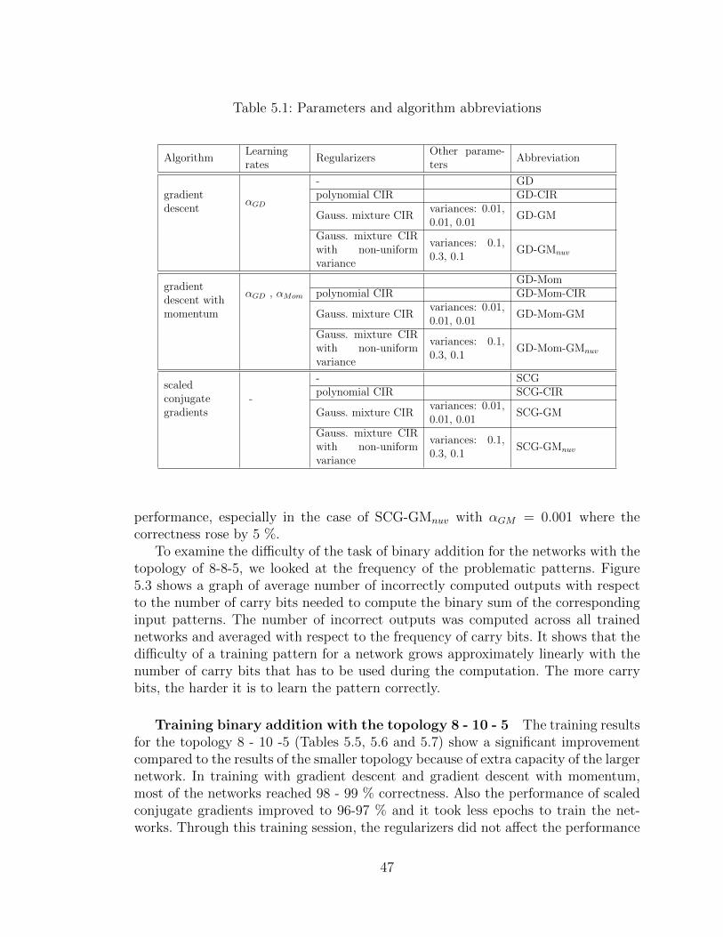
Table 5.1: Parameters and algorithm abbreviations

AlgorithmLearningrates

RegularizersOther parame-ters

Abbreviation

gradientdescent

αGD

- GDpolynomial CIR GD-CIR

Gauss. mixture CIRvariances: 0.01,0.01, 0.01

GD-GM

Gauss. mixture CIRwith non-uniformvariance

variances: 0.1,0.3, 0.1

GD-GMnuv

gradientdescent withmomentum

αGD , αMom

GD-Mompolynomial CIR GD-Mom-CIR

Gauss. mixture CIRvariances: 0.01,0.01, 0.01

GD-Mom-GM

Gauss. mixture CIRwith non-uniformvariance

variances: 0.1,0.3, 0.1

GD-Mom-GMnuv

scaledconjugategradients

-

- SCGpolynomial CIR SCG-CIR

Gauss. mixture CIRvariances: 0.01,0.01, 0.01

SCG-GM

Gauss. mixture CIRwith non-uniformvariance

variances: 0.1,0.3, 0.1

SCG-GMnuv

performance, especially in the case of SCG-GMnuv with αGM = 0.001 where thecorrectness rose by 5 %.

To examine the difficulty of the task of binary addition for the networks with thetopology of 8-8-5, we looked at the frequency of the problematic patterns. Figure5.3 shows a graph of average number of incorrectly computed outputs with respectto the number of carry bits needed to compute the binary sum of the correspondinginput patterns. The number of incorrect outputs was computed across all trainednetworks and averaged with respect to the frequency of carry bits. It shows that thedifficulty of a training pattern for a network grows approximately linearly with thenumber of carry bits that has to be used during the computation. The more carrybits, the harder it is to learn the pattern correctly.

Training binary addition with the topology 8 - 10 - 5 The training resultsfor the topology 8 - 10 -5 (Tables 5.5, 5.6 and 5.7) show a significant improvementcompared to the results of the smaller topology because of extra capacity of the largernetwork. In training with gradient descent and gradient descent with momentum,most of the networks reached 98 - 99 % correctness. Also the performance of scaledconjugate gradients improved to 96-97 % and it took less epochs to train the net-works. Through this training session, the regularizers did not affect the performance

47

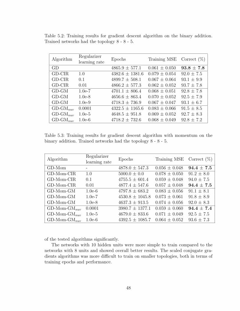
Table 5.2: Training results for gradient descent algorithm on the binary addition.Trained networks had the topology 8 - 8 - 5.

AlgorithmRegularizerlearning rate

Epochs Training MSE Correct (%)

GD 4865.9 ± 577.1 0.061 ± 0.050 93.8 ± 7.8GD-CIR 1.0 4382.6 ± 1381.6 0.079 ± 0.054 92.0 ± 7.5GD-CIR 0.1 4899.7 ± 508.1 0.067 ± 0.064 93.1 ± 9.9GD-CIR 0.01 4866.2 ± 577.3 0.062 ± 0.052 93.7 ± 7.8GD-GM 1.0e-7 4701.1 ± 806.4 0.068 ± 0.051 92.8 ± 7.8GD-GM 1.0e-8 4656.6 ± 863.4 0.070 ± 0.052 92.5 ± 7.9GD-GM 1.0e-9 4718.3 ± 736.9 0.067 ± 0.047 93.1 ± 6.7GD-GMnuv 0.0001 4322.5 ± 1165.6 0.083 ± 0.066 91.5 ± 8.5GD-GMnuv 1.0e-5 4648.5 ± 951.8 0.069 ± 0.052 92.7 ± 8.3GD-GMnuv 1.0e-6 4718.2 ± 732.6 0.068 ± 0.049 92.8 ± 7.2

Table 5.3: Training results for gradient descent algorithm with momentum on thebinary addition. Trained networks had the topology 8 - 8 - 5.

AlgorithmRegularizerlearning rate

Epochs Training MSE Correct (%)

GD-Mom - 4878.0 ± 547.3 0.056 ± 0.048 94.4 ± 7.5GD-Mom-CIR 1.0 5000.0 ± 0.0 0.078 ± 0.050 91.2 ± 8.0GD-Mom-CIR 0.1 4755.5 ± 601.4 0.059 ± 0.048 94.0 ± 7.5GD-Mom-CIR 0.01 4877.4 ± 547.6 0.057 ± 0.048 94.4 ± 7.5GD-Mom-GM 1.0e-6 4797.8 ± 683.2 0.083 ± 0.056 91.1 ± 8.1GD-Mom-GM 1.0e-7 4530.8 ± 1045.8 0.073 ± 0.061 91.8 ± 8.9GD-Mom-GM 1.0e-8 4637.3 ± 913.5 0.074 ± 0.056 92.0 ± 8.3GD-Mom-GMnuv 0.0001 3980.7 ± 1377.1 0.059 ± 0.060 94.4 ± 7.4GD-Mom-GMnuv 1.0e-5 4679.0 ± 833.6 0.071 ± 0.049 92.5 ± 7.5GD-Mom-GMnuv 1.0e-6 4392.5 ± 1085.7 0.064 ± 0.052 93.6 ± 7.3

of the tested algorithms significantly.The networks with 10 hidden units were more simple to train compared to the

networks with 8 units and showed overall better results. The scaled conjugate gra-dients algorithms was more difficult to train on smaller topologies, both in terms oftraining epochs and performance.

48

Table 5.4: Training results for scaled conjugate gradients algorithm on the binaryaddition. Trained networks had the topology 8 - 8 - 5.

AlgorithmRegularizerlearning rate

Epochs Training MSE Correct (%)

SCG 4583.4 ± 1257.1 0.099 ± 0.050 90.7 ± 4.9SCG-CIR 0.1 3694.2 ± 1961.5 0.086 ± 0.078 91.6 ± 9.1SCG-CIR 0.01 4133.3 ± 1648.5 0.079 ± 0.048 92.4 ± 5.4SCG-CIR 0.001 4326.7 ± 1552.0 0.093 ± 0.067 90.7 ± 8.5SCG-GM 1.0e-5 4266.3 ± 1630.0 0.084 ± 0.051 91.9 ± 5.8SCG-GM 1.0e-6 4561.2 ± 1270.1 0.103 ± 0.068 89.0 ± 8.4SCG-GM 1.0e-7 4271.6 ± 1618.1 0.079 ± 0.046 92.2 ± 5.5SCG-GMnuv 0.001 3469.0 ± 2099.9 0.060 ± 0.057 95.1 ± 5.7SCG-GMnuv 0.0001 4225.3 ± 1549.0 0.068 ± 0.040 93.2 ± 5.8SCG-GMnuv 1.0e-5 4478.8 ± 1360.8 0.085 ± 0.044 92.0 ± 4.4

0 1 2 3 40

100

200

300

400

500

600

Number of carry bits

Ave

rage

num

ber

of in

corr

ect r

esul

ts

Figure 5.3: Average number of incorrect results for input patterns with respect tothe number of carry bits in the pattern for binary addition.

Performance on noisy data To estimate the robustness of networks trainedby each of the tested algorithm, their performance was measured on sets of noisy data.Tables 5.8 and 5.9 show the results for both presented network’s architectures. Theperformance was measured with respect to the data with artificially added uniformlydistributed noise with magnitude of 5 and 10 %.

49

Table 5.5: Training results for gradient descent algorithm on the binary addition.Trained networks had the topology 8 - 10 - 5.

AlgorithmRegularizerlearning rate

Epochs Training MSE Correct (%)

GD 3096.8 ± 1666.7 0.019 ± 0.019 98.9 ± 2.2GD-CIR 0.1 2829.5 ± 1668.5 0.015 ± 0.013 99.3 ± 1.7GD-CIR 0.01 3028.1 ± 1651.4 0.017 ± 0.018 99.1 ± 2.0GD-GM 1.0e-7 3154.0 ± 1785.0 0.024 ± 0.022 98.3 ± 2.5GD-GM 1.0e-8 2903.7 ± 1748.7 0.022 ± 0.023 98.6 ± 2.5GD-GMnuv 0.0001 2598.1 ± 1373.3 0.017 ± 0.019 99.1 ± 2.2GD-GMnuv 1.0e-5 3319.9 ± 1722.4 0.023 ± 0.021 98.4 ± 2.4

Table 5.6: Training results for gradient descent algorithm with momentum on thebinary addition. Trained networks had the topology 8 - 10 - 5.

AlgorithmRegularizerlearning rate

Epochs Training MSE Correct (%)

GD-Mom 2756.2 ± 1708.2 0.017 ± 0.017 99.0 ± 2.2GD-Mom-CIR 0.1 2811.7 ± 1668.5 0.019 ± 0.019 98.8 ± 2.2GD-Mom-CIR 0.01 2734.5 ± 1722.5 0.016 ± 0.015 99.1 ± 1.8GD-Mom-GM 0.0001 5000.0 ± 0.0 0.367 ± 0.104 55.5 ± 12.4GD-Mom-GM 1.0e-5 4282.0 ± 1428.9 0.040 ± 0.025 96.7 ± 2.6GD-Mom-GMnuv 0.0001 2728.5 ± 1621.1 0.023 ± 0.024 98.5 ± 2.7GD-Mom-GMnuv 1.0e-5 2695.0 ± 1767.9 0.021 ± 0.023 98.8 ± 2.5

The first Table 5.8 shows the results for the 8-8-5 architecture. During training,the best performance was achieved by training with standard gradient descent andgradient descent with momentum. However, these results deteriorated quickly onthe noisy data. In both cases, the algorithms with internal representations enforcedby the Gaussian mixture model with non-uniform variance GMnuv exhibited thebest robustness against noisy data. Also in case of scaled conjugate gradients, thisalgorithm performed the best.

A similar trend can be seen from the results from the 8 - 10 - 5 architecture 5.9.The performance on the original data set was approximately similar for all the testedalgorithms. On the noisy data, again the algorithms with GMnuv regularizer reachedthe best performance.

50

Table 5.7: Training results for scaled conjugate gradients algorithm on the binaryaddition. Trained networks had the topology 8 - 10 - 5.

AlgorithmRegularizerlearning rate

Epochs Training MSE Correct (%)

SCG 2611.6 ± 2058.9 0.028 ± 0.029 97.6 ± 3.1SCG-CIR 0.1 2914.9 ± 2098.6 0.031 ± 0.027 97.3 ± 3.0SCG-CIR 0.01 3203.4 ± 2113.4 0.034 ± 0.031 96.8 ± 3.3SCG-GM 0.0001 4424.8 ± 1498.7 0.098 ± 0.170 90.3 ± 13.5SCG-GM 1.0e-5 3506.3 ± 2024.2 0.040 ± 0.032 96.3 ± 3.4SCG-GMnuv 0.001 2834.0 ± 2232.4 0.032 ± 0.030 97.6 ± 3.3SCG-GMnuv 0.0001 2948.2 ± 2171.1 0.038 ± 0.040 96.7 ± 4.1

Analysis of formed internal representations - gradient descent The BP-networks with enforced internal representations showed generally better performanceand generalization capabilities, especially on noisy data. To examine, how the con-densed internal representations contribute to the performance of the networks, weshall now analyse internal representations formed in some of the successfully trainednetworks.

This section closely analyses internal representations of networks with 8 hiddenneurons that were trained by the GD algorithm, either with enforced internal repre-sentation or without it. These networks were selected for analysis because both theresults in the training and performance on noisy data showed the largest differencebetween the networks trained by standard GD and GD with GMnuv-enforced internalrepresentations.

Figure 5.4 shows the internal representations of the training set formed by theGD algorithm in a visual form, the rows represent individual internal representationsand the squares in each row represent the activation of a neuron in the hiddenlayer on a scale from black (passive state) to white (active state). The internalrepresentations are sorted according to their similarity (as measured by Euclideandistance between vectors of internal representations). The colours that surround eachinternal representation represent the number of carry bits in the computation of sumof two numbers.

As we can see, the activations do not show large variability, however there are noredundant neurons in the terms specified in Section 4.5. The similarity of internalrepresentations does not follow the distribution of carry bits. Only the patterns with0 carry bits are partially grouped together (blue regions on the left).

Compare the figure for GD with Figure 5.5, where the internal representationsformed by GD-GMnuv are displayed. Again, the internal representations are sortedaccording to their similarity. This time, the regions of patterns with the same numberof carry bits are more separated from each other and less discontinuous.

51

Table 5.8: Performance of networks trained with the tested algorithms on noisy data.The networks had the topology 8 - 8 - 5 and were trained on binary addition.

AlgorithmRegularizerlearning rate

Average num-ber of correctadditions(originaldata)

Average num-ber of correctadditions - 5% noise

Average num-ber of correctadditions - 10% noise

GD 93.8 ± 7.8 88.0 ± 8.5 75.4 ± 8.3GD-CIR 1.0 92.0 ± 7.5 87.7 ± 9.0 76.9 ± 10.2GD-CIR 0.1 93.1 ± 9.9 87.1 ± 10.6 74.7 ± 9.7GD-CIR 0.01 93.7 ± 7.8 88.0 ± 8.5 75.4 ± 8.2GD-GM 1.0e-7 92.8 ± 7.8 88.2 ± 8.7 76.5 ± 9.1GD-GM 1.0e-8 92.5 ± 7.9 88.0 ± 8.8 76.3 ± 9.0GD-GM 1.0e-9 93.1 ± 6.7 88.5 ± 7.8 76.9 ± 8.1GD-GMnuv 0.0001 91.5 ± 8.5 87.8 ± 9.2 80.2 ± 9.7GD-GMnuv 1.0e-5 92.7 ± 8.3 88.5 ± 9.2 78.1 ± 9.2GD-GMnuv 1.0e-6 92.8 ± 7.2 88.6 ± 8.2 76.8 ± 8.9

GD-Mom 94.4 ± 7.5 89.6 ± 8.6 75.3 ± 8.0GD-Mom-CIR 1.0 91.2 ± 8.0 86.6 ± 9.3 74.3 ± 9.1GD-Mom-CIR 0.1 94.0 ± 7.5 89.1 ± 8.7 75.5 ± 8.2GD-Mom-CIR 0.01 94.4 ± 7.5 89.6 ± 8.7 75.3 ± 8.1GD-Mom-GM 1.0e-6 91.1 ± 8.1 86.4 ± 8.7 75.3 ± 8.5GD-Mom-GM 1.0e-7 91.8 ± 8.9 86.8 ± 10.3 75.6 ± 10.5GD-Mom-GM 1.0e-8 92.0 ± 8.3 87.1 ± 9.5 76.0 ± 9.2GD-Mom-GMnuv 0.0001 94.4 ± 7.4 90.7 ± 8.5 83.0 ± 9.1GD-Mom-GMnuv 1.0e-5 92.5 ± 7.5 87.6 ± 8.6 76.4 ± 8.8GD-Mom-GMnuv 1.0e-6 93.6 ± 7.3 88.8 ± 8.7 77.0 ± 8.8

SCG 90.7 ± 4.9 80.4 ± 9.3 69.3 ± 9.1SCG-CIR 0.1 91.6 ± 9.1 81.2 ± 13.7 69.3 ± 12.7SCG-CIR 0.01 92.4 ± 5.4 82.1 ± 8.5 69.8 ± 9.3SCG-CIR 0.001 90.7 ± 8.5 78.6 ± 12.5 67.8 ± 11.2SCG-GM 1.0e-5 91.9 ± 5.8 81.3 ± 7.0 70.1 ± 8.5SCG-GM 1.0e-6 89.0 ± 8.4 77.7 ± 12.3 66.9 ± 12.3SCG-GM 1.0e-7 92.2 ± 5.5 83.1 ± 7.1 71.6 ± 8.9SCG-GMnuv 0.001 95.1 ± 5.7 89.1 ± 5.9 81.3 ± 6.4SCG-GMnuv 0.0001 93.2 ± 5.8 85.7 ± 7.1 73.8 ± 7.7SCG-GMnuv 1.0e-5 92.0 ± 4.4 82.3 ± 7.4 70.6 ± 7.9

52

Table 5.9: Performance of networks trained with the tested algorithms on noisy data.The networks had the topology 8 - 10 - 5 and were trained on binary addition.

AlgorithmRegularizerlearningrate

Average num-ber of correctadditions(original data)

Average num-ber of correctadditions - 5% noise

Average num-ber of correctadditions - 10% noise

GD 98.9 ± 2.2 96.1 ± 3.9 87.8 ± 6.1GD-CIR 0.1 99.3 ± 1.7 96.1 ± 4.2 87.8 ± 6.5GD-CIR 0.01 99.1 ± 2.0 96.2 ± 4.0 88.0 ± 6.0GD-GM 1.0e-7 98.3 ± 2.5 95.3 ± 4.0 86.4 ± 6.2GD-GM 1.0e-8 98.6 ± 2.5 95.8 ± 4.0 88.0 ± 5.5GD-GMnuv 0.000 99.1 ± 2.2 96.7 ± 3.1 90.5 ± 3.9GD-GMnuv 0.000 98.4 ± 2.4 95.2 ± 3.9 87.0 ± 5.2

GD-Mom 99.0 ± 2.2 95.7 ± 4.3 87.4 ± 6.5GD-Mom-CIR 0.1 98.8 ± 2.2 95.4 ± 4.0 87.4 ± 5.5GD-Mom-CIR 0.01 99.1 ± 1.8 95.9 ± 4.0 87.5 ± 6.2GD-Mom-GM 0.0001 55.5 ± 12.4 50.3 ± 11.6 44.5 ± 10.6GD-Mom-GM 1.0e-5 96.7 ± 2.6 91.9 ± 4.6 81.1 ± 6.2GD-Mom-GMnuv 0.0001 98.5 ± 2.7 96.2 ± 3.8 90.2 ± 4.6GD-Mom-GMnuv 1.0e-5 98.8 ± 2.5 95.8 ± 3.6 87.8 ± 5.4

SCG 97.6 ± 3.1 90.1 ± 4.5 78.3 ± 7.5SCG-CIR 0.1 97.3 ± 3.0 89.9 ± 4.6 79.6 ± 7.4SCG-CIR 0.01 96.8 ± 3.3 89.8 ± 4.0 79.6 ± 6.7SCG-GM 0.0001 90.3 ± 13.5 81.0 ± 13.2 70.8 ± 12.1SCG-GM 1.0e-5 96.3 ± 3.4 88.5 ± 4.4 77.6 ± 6.7SCG-GMnuv 0.001 97.6 ± 3.3 92.4 ± 3.9 84.0 ± 5.3SCG-GMnuv 0.0001 96.7 ± 4.1 91.2 ± 3.7 81.7 ± 5.2

To further analyse the groups which are formed by similar internal representa-tions, self-organizing maps (SOM) were trained on the internal representations shownin the previous figures. Self-organizing maps had 7 × 7 units organized in hexag-onal topology. The map trained on the internal representations formed by the GDalgorithm is displayed in Figures 5.6 and 5.7. The first figure shows the distancesof adjacent units in the SOM, light colours represent small distances, darker colourslarger distances. There are some regions of units relatively close to each other whichdefine clusters.

The Figure 5.7 shows the mapping of internal representations into the trainedSOM. Each hexagon represent a unit in the map, the number inside the hexagonspecifies the number of internal representations that were mapped into the unit. Thecolor is determined by the number of carry bits of the patterns mapped into the

53

passive silent active

Activations

Number of carry bits

0

1

2

3

4

Figure 5.4: Internal representations formed in a BP-network with 8-8-5 topologytrained by gradient descent GD on the binary addition task. The internal represen-tations are sorted according to their similarity. White color represents active neurons(with activation 1), black color corresponds to silent networks (activation 0), othervalues of activations are displayed on grayscale. The colours that surround each in-ternal representation specify the number of carry bits in the computation of sum oftwo numbers.

same unit. The colours are also scaled with respect to the ratio of different numbersof carry bits mapped into the unit. When different numbers of carry bits are mappedonto the same unit uniformly, the unit has grey colour.

For the network trained by gradient descent (GD), the mapping into the SOM5.6 shows groups of blue units in the left part. The other parts of the map are mostlygreyish which means that patterns with different numbers of carry bits were mappedinto the same units. The clusters formed in the SOM by neighbour distances do notcorrespond well to these groups.

By comparison with the internal representations from Figure 5.4, indeed the re-gions are more continuous than other regions, i. e. internal representations of patternswith no carry bits were similar. This means that the network trained by GD wasable to identify the patterns with no carry bits, other patterns shared mostly similarinternal representations and this lead to deteriorated performance on noisy data.

Figures 5.8 and 5.9 shows the SOM trained on internal representations formed

54

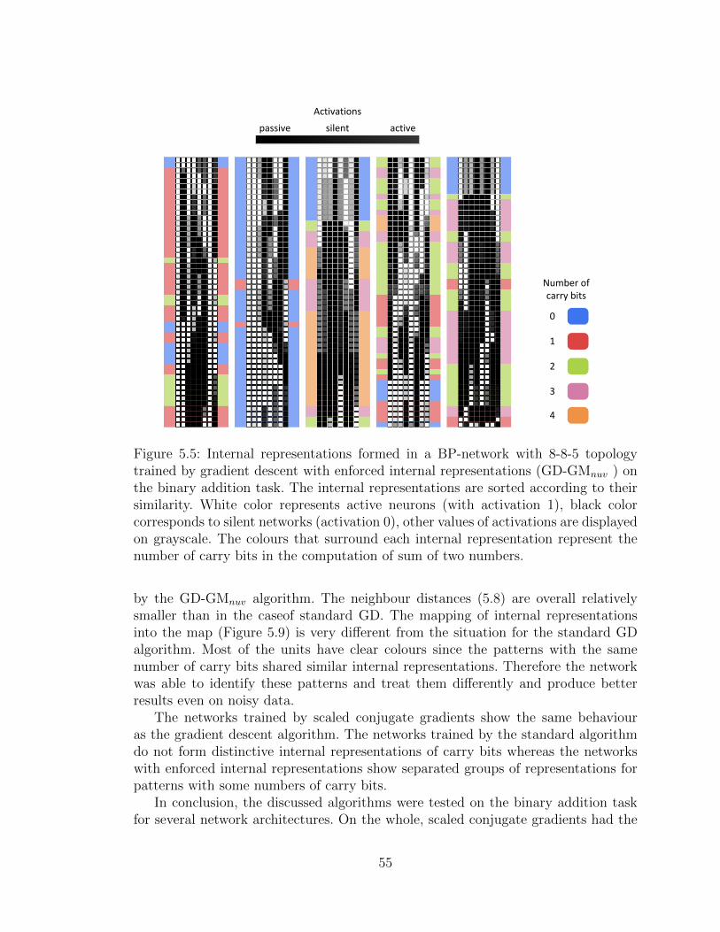
passive silent active

Activations

Number of carry bits

0

1

2

3

4

Figure 5.5: Internal representations formed in a BP-network with 8-8-5 topologytrained by gradient descent with enforced internal representations (GD-GMnuv ) onthe binary addition task. The internal representations are sorted according to theirsimilarity. White color represents active neurons (with activation 1), black colorcorresponds to silent networks (activation 0), other values of activations are displayedon grayscale. The colours that surround each internal representation represent thenumber of carry bits in the computation of sum of two numbers.

by the GD-GMnuv algorithm. The neighbour distances (5.8) are overall relativelysmaller than in the caseof standard GD. The mapping of internal representationsinto the map (Figure 5.9) is very different from the situation for the standard GDalgorithm. Most of the units have clear colours since the patterns with the samenumber of carry bits shared similar internal representations. Therefore the networkwas able to identify these patterns and treat them differently and produce betterresults even on noisy data.

The networks trained by scaled conjugate gradients show the same behaviouras the gradient descent algorithm. The networks trained by the standard algorithmdo not form distinctive internal representations of carry bits whereas the networkswith enforced internal representations show separated groups of representations forpatterns with some numbers of carry bits.

In conclusion, the discussed algorithms were tested on the binary addition taskfor several network architectures. On the whole, scaled conjugate gradients had the

55

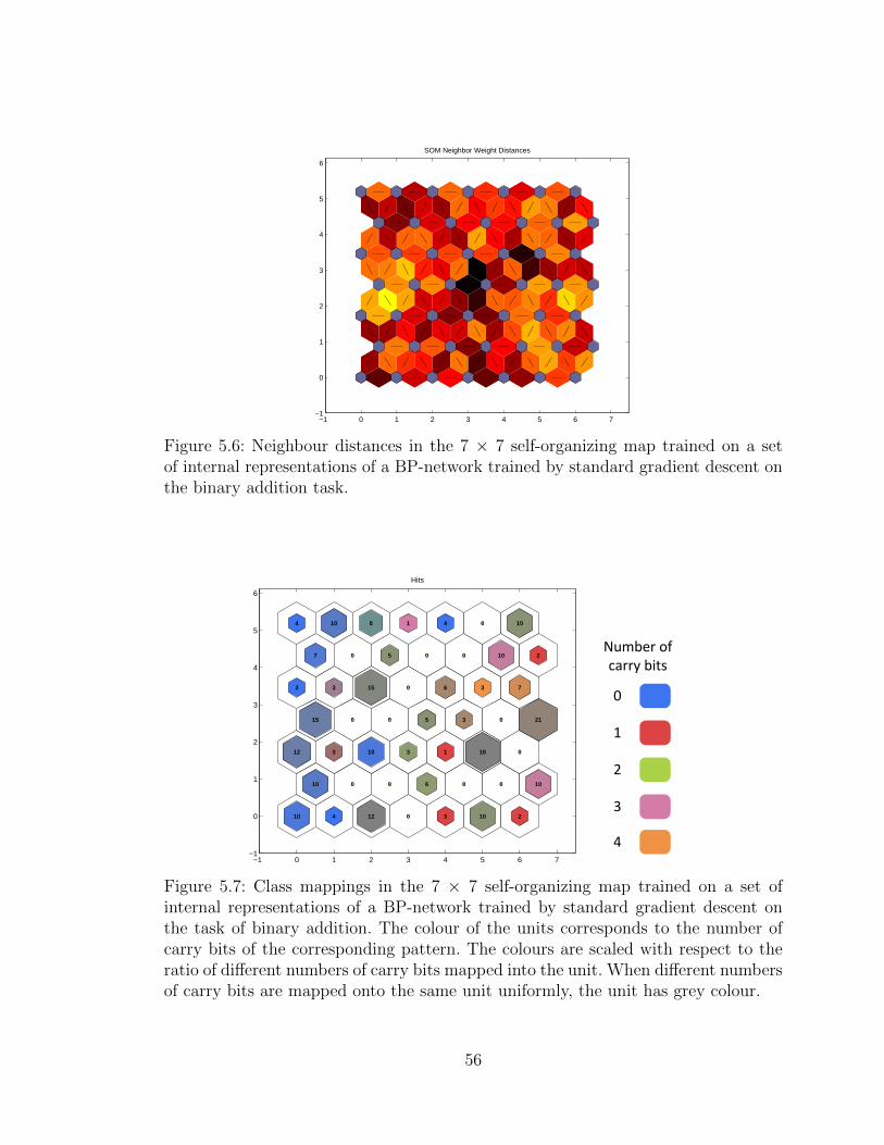
−1 0 1 2 3 4 5 6 7−1

0

1

2

3

4

5

6

SOM Neighbor Weight Distances

Figure 5.6: Neighbour distances in the 7 × 7 self-organizing map trained on a setof internal representations of a BP-network trained by standard gradient descent onthe binary addition task.

−1 0 1 2 3 4 5 6 7−1

0

1

2

3

4

5

6

10 4 12 0 3 10 2

10 0 0 6 0 0 10

12 3 10 3 1 18 0

15 0 0 5 3 0 21

3 3 15 0 6 3 7

7 0 5 0 0 10 2

4 10 8 1 4 0 10

Hits

Number of carry bits

0

1

2

3

4

Figure 5.7: Class mappings in the 7 × 7 self-organizing map trained on a set ofinternal representations of a BP-network trained by standard gradient descent onthe task of binary addition. The colour of the units corresponds to the number ofcarry bits of the corresponding pattern. The colours are scaled with respect to theratio of different numbers of carry bits mapped into the unit. When different numbersof carry bits are mapped onto the same unit uniformly, the unit has grey colour.

56

−1 0 1 2 3 4 5 6 7−1

0

1

2

3

4

5

6

SOM Neighbor Weight Distances

Figure 5.8: Neighbour distances in the 7 × 7 self-organizing map trained on a set ofinternal representations of a BP-network trained by gradient descent with enforcedinternal representations GD-GMnuv on the binary addition task.

−1 0 1 2 3 4 5 6 7−1

0

1

2

3

4

5

6

5 6 6 4 8 6 4

8 4 4 4 8 5 8

8 0 1 4 2 4 4

4 7 8 4 6 2 2

12 2 1 4 4 4 8

8 3 4 4 8 8 2

8 8 1 8 8 5 10

Hits

Number of carry bits

0

1

2

3

4

Figure 5.9: Class mappings in the 7 × 7 self-organizing map trained on a set ofinternal representations of a BP-network trained by gradient descent with enforcedinternal representations GD-GMnuv on the binary addition task. The colour of theunits corresponds to the number of carry bits of the corresponding pattern. Thecolours are scaled with respect to the ratio of different numbers of carry bits mappedinto the unit. When different numbers of carry bits are mapped onto the same unituniformly, the unit has grey colour.

57

largest difficulty with learning the task, gradient descent and gradient descent withmomentum achieved very good performance. Among the tested algorithms, the bestresults with respect to noisy data were achieved by training with internal repre-sentation enforced by the Gaussian mixture model (Section 4.7) with non-uniformvariances.

An analysis of internal representations formed during training showed that moresuccessful networks were able to identify and treat different types of the input pat-terns - depending on the number of carry bits needed to perform the addition ofbinary numbers.

58

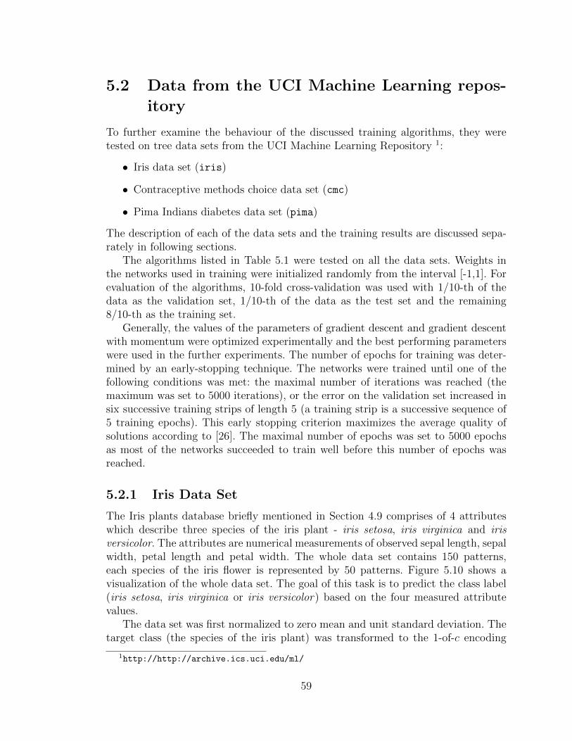
5.2 Data from the UCI Machine Learning repos-

itory

To further examine the behaviour of the discussed training algorithms, they weretested on tree data sets from the UCI Machine Learning Repository 1:

• Iris data set (iris)

• Contraceptive methods choice data set (cmc)

• Pima Indians diabetes data set (pima)

The description of each of the data sets and the training results are discussed sepa-rately in following sections.

The algorithms listed in Table 5.1 were tested on all the data sets. Weights inthe networks used in training were initialized randomly from the interval [-1,1]. Forevaluation of the algorithms, 10-fold cross-validation was used with 1/10-th of thedata as the validation set, 1/10-th of the data as the test set and the remaining8/10-th as the training set.

Generally, the values of the parameters of gradient descent and gradient descentwith momentum were optimized experimentally and the best performing parameterswere used in the further experiments. The number of epochs for training was deter-mined by an early-stopping technique. The networks were trained until one of thefollowing conditions was met: the maximal number of iterations was reached (themaximum was set to 5000 iterations), or the error on the validation set increased insix successive training strips of length 5 (a training strip is a successive sequence of5 training epochs). This early stopping criterion maximizes the average quality ofsolutions according to [26]. The maximal number of epochs was set to 5000 epochsas most of the networks succeeded to train well before this number of epochs wasreached.

5.2.1 Iris Data Set

The Iris plants database briefly mentioned in Section 4.9 comprises of 4 attributeswhich describe three species of the iris plant - iris setosa, iris virginica and irisversicolor. The attributes are numerical measurements of observed sepal length, sepalwidth, petal length and petal width. The whole data set contains 150 patterns,each species of the iris flower is represented by 50 patterns. Figure 5.10 shows avisualization of the whole data set. The goal of this task is to predict the class label(iris setosa, iris virginica or iris versicolor) based on the four measured attributevalues.

The data set was first normalized to zero mean and unit standard deviation. Thetarget class (the species of the iris plant) was transformed to the 1-of-c encoding

1http://http://archive.ics.uci.edu/ml/

59

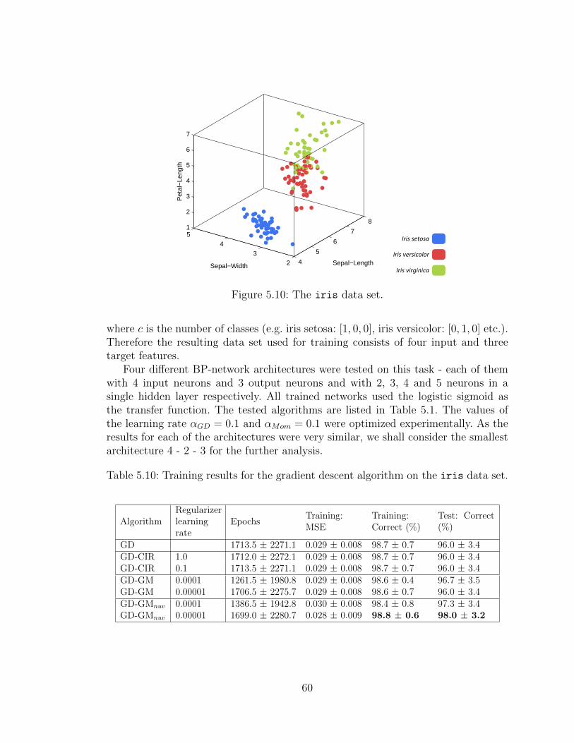
4

5

6

7

8

23

451

2

3

4

5

6

7

Sepal−LengthSepal−Width

Pet

al−

Leng

th

Iris setosa

Iris versicolor

Iris virginica

Figure 5.10: The iris data set.

where c is the number of classes (e.g. iris setosa: [1, 0, 0], iris versicolor: [0, 1, 0] etc.).Therefore the resulting data set used for training consists of four input and threetarget features.

Four different BP-network architectures were tested on this task - each of themwith 4 input neurons and 3 output neurons and with 2, 3, 4 and 5 neurons in asingle hidden layer respectively. All trained networks used the logistic sigmoid asthe transfer function. The tested algorithms are listed in Table 5.1. The values ofthe learning rate αGD = 0.1 and αMom = 0.1 were optimized experimentally. As theresults for each of the architectures were very similar, we shall consider the smallestarchitecture 4 - 2 - 3 for the further analysis.

Table 5.10: Training results for the gradient descent algorithm on the iris data set.

AlgorithmRegularizerlearningrate

EpochsTraining:MSE

Training:Correct (%)

Test: Correct(%)

GD 1713.5 ± 2271.1 0.029 ± 0.008 98.7 ± 0.7 96.0 ± 3.4

GD-CIR 1.0 1712.0 ± 2272.1 0.029 ± 0.008 98.7 ± 0.7 96.0 ± 3.4GD-CIR 0.1 1713.5 ± 2271.1 0.029 ± 0.008 98.7 ± 0.7 96.0 ± 3.4

GD-GM 0.0001 1261.5 ± 1980.8 0.029 ± 0.008 98.6 ± 0.4 96.7 ± 3.5GD-GM 0.00001 1706.5 ± 2275.7 0.029 ± 0.008 98.6 ± 0.7 96.0 ± 3.4

GD-GMnuv 0.0001 1386.5 ± 1942.8 0.030 ± 0.008 98.4 ± 0.8 97.3 ± 3.4GD-GMnuv 0.00001 1699.0 ± 2280.7 0.028 ± 0.009 98.8 ± 0.6 98.0 ± 3.2

60

Table 5.11: Training results for the gradient descent algorithm with momentum onthe iris data set.

AlgorithmRegularizerlearningrate

EpochsTraining:MSE

Training:Correct (%)

Test: Correct(%)

GD-Mom 1696.0 ± 2282.8 0.029 ± 0.008 98.6 ± 0.7 96.0 ± 3.4

GD-Mom-CIR 1.0 1695.0 ± 2283.5 0.029 ± 0.008 98.6 ± 0.7 96.0 ± 3.4GD-Mom-CIR 0.1 1696.0 ± 2282.8 0.029 ± 0.008 98.6 ± 0.7 96.0 ± 3.4

GD-Mom-GM 0.0001 1244.5 ± 1988.9 0.029 ± 0.008 98.6 ± 0.7 96.7 ± 3.5GD-Mom-GM 0.00001 1689.5 ± 2287.1 0.029 ± 0.008 98.7 ± 0.7 96.0 ± 3.4

GD-Mom-GMnuv 0.0001 1699.0 ± 2280.1 0.030 ± 0.008 98.8 ± 0.6 97.3 ± 3.4GD-Mom-GMnuv 0.00001 1673.0 ± 2297.2 0.028 ± 0.009 98.6 ± 0.6 96.7 ± 3.5

Table 5.12: Training results for the scaled conjugate gradients algorithm on the irisdata

AlgorithmRegularizerlearningrate

EpochsTraining:MSE

Training:Correct (%)

Test: Correct(%)

SCG 572.0 ± 742.4 0.042 ± 0.100 96.3 ± 9.9 92.7 ± 10.2

SCG-CIR 1.0 309.5 ± 373.1 0.043 ± 0.099 96.3 ± 9.8 92.7 ± 10.6SCG-CIR 0.1 156.5 ± 111.3 0.044 ± 0.100 96.3 ± 9.8 92.0 ± 10.3

SCG-GM 0.0001 119.5 ± 85.2 0.044 ± 0.099 96.3 ± 9.9 92.7 ± 10.2SCG-GM 0.00001 153.5 ± 116.0 0.046 ± 0.104 96.3 ± 9.8 92.0 ± 10.3

SCG-GMnuv 0.0001 131.0 ± 84.0 0.045 ± 0.099 96.3 ± 9.8 92.7 ± 10.6SCG-GMnuv 0.00001 114.5 ± 62.0 0.047 ± 0.109 96.3 ± 9.8 92.0 ± 10.3

Experimental results An overview of the training results for BP-networkswith two neurons in the hidden layer is given in Tables 5.10, 5.11 and 5.12. Thecolumn Algorithm represents the abbreviations of training algorithms presented inTable 5.1, Epochs show the average number of training epochs together with standarddeviation, the column Training: MSE represents the mean squared error reached dur-ing training and the remaining columns show the average correctness of classificationfor the training and test sets, respectively. The results of other tested architectureswere very similar.

The performance of gradient descent (GD, Table 5.10) and gradient descent withmomentum (GD-Mom,Table 5.11) was very similar, regardless of the usage of en-forced internal representations. Scaled conjugate gradients (SCG, Table 5.12) showedslightly worse performance, their correctness on the test set was approximately 4 %lower than GD and GD-Mom. Again, the performance stayed approximately thesame regardless of the method used.

61

−1 0 1 2 3 4 5−1

−0.5

0

0.5

1

1.5

2

2.5

3

3.5

4

SOM Neighbor Weight Distances

Figure 5.11: Neighbour distances in the 5 × 5 self-organizing map trained on a setof internal representations of a BP-network trained by standard gradient descent onthe iris data set

The only exception which showed better performance are the networks with in-ternal representations enforced by the Gaussian mixture model with non-uniformvariance. In case of the gradient descent optimization 5.10, the correctness on thetest set was 2 % higher than the standard gradient descent. Similarly for the gradi-ent descent with momentum 5.11, the correctness on the test set was 1.3 % higherthan the standard algorithm and 0.6 % higher than other results. Only for the scaledconjugate gradients, the performance of all the algorithms was approximately thesame.

Analysis of internal representations To further examine the internal repre-sentations formed during training and their relevance to the performance, the internalrepresentations formed in the standard gradient descent (GD) and in the gradientdescent with internal representations enforced by the mixture of Gaussians with non-uniform variance (GD-GMnuv) were compared. These two algorithms were selectedbecause they showed the largest difference in performance (Table5.10). One networktrained by each of the two algorithm was selected for the analysis, the network wastrained on the same set of training patterns during the cross-validation to ensurecomparability of the results. The internal representations formed during the cross-validation were extracted for both algorithms.

A self-organizing map (SOM) was trained on these internal representations toidentify potential clusters. Figures 5.11 and 5.13 show the the distances betweenneighbouring neurons in the trained self-organizing map with 5 × 5 units in a hexag-onal topology. Lighter colour represent small distances, the darker the colour is, the

62

−1 0 1 2 3 4 5−1

−0.5

0

0.5

1

1.5

2

2.5

3

3.5

4

32 3 1 6 28

14 0 0 1 2

0 0 0 2 1

38 3 1 1 2

7 0 2 3 3

Hits

Iris setosa

Iris versicolor

Iris virginica

Figure 5.12: Class mappings in the 5 × 5 self-organizing map trained on a set ofinternal representations of a BP-network trained by standard gradient descent onthe iris data set. The colour of the units corresponds to the class attribute withrespect to the ratio of classes mapped into the unit. When different classes aremapped onto the same unit uniformly, the unit has grey colour.

−1 0 1 2 3 4 5−1

−0.5

0

0.5

1

1.5

2

2.5

3

3.5

4

SOM Neighbor Weight Distances

Figure 5.13: Neighbour distances in the 5 × 5 self-organizing map trained on a set ofinternal representations of a BP-network trained by gradient descent with internalrepresentations enforced by a Gaussian mixture model with non-uniform variance onthe iris data set

63

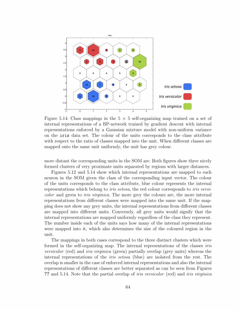
−1 0 1 2 3 4 5−1

−0.5

0

0.5

1

1.5

2

2.5

3

3.5

4

5 22 2 0 0

13 7 1 0 3

0 0 0 0 8

4 8 3 2 33

9 24 1 3 2

Hits

Iris setosa

Iris versicolor

Iris virginica

Figure 5.14: Class mappings in the 5 × 5 self-organizing map trained on a set ofinternal representations of a BP-network trained by gradient descent with internalrepresentations enforced by a Gaussian mixture model with non-uniform varianceon the iris data set. The colour of the units corresponds to the class attributewith respect to the ratio of classes mapped into the unit. When different classes aremapped onto the same unit uniformly, the unit has grey colour.

more distant the corresponding units in the SOM are. Both figures show three nicelyformed clusters of very proximate units separated by regions with larger distances.

Figures 5.12 and 5.14 show which internal representations are mapped to eachneuron in the SOM given the class of the corresponding input vector. The colourof the units corresponds to the class attribute, blue colour represents the internalrepresentations which belong to iris setosa, the red colour corresponds to iris versi-color and green to iris virginica. The more grey the colours are, the more internalrepresentations from different classes were mapped into the same unit. If the map-ping does not show any grey units, the internal representations from different classesare mapped into different units. Conversely, all grey units would signify that theinternal representations are mapped uniformly regardless of the class they represent.The number inside each of the units says how many of the internal representationswere mapped into it, which also determines the size of the coloured region in theunit.

The mappings in both cases correspond to the three distinct clusters which wereformed in the self-organizing map. The internal representations of the classes irisversicolor (red) and iris virginica (green) partially overlap (grey units) whereas theinternal representations of the iris setosa (blue) are isolated from the rest. Theoverlap is smaller in the case of enforced internal representations and also the internalrepresentations of different classes are better separated as can be seen from Figures?? and 5.14. Note that the partial overlap of iris versicolor (red) and iris virginica

64

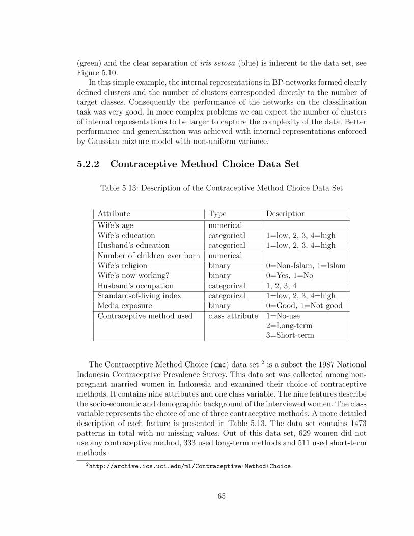
(green) and the clear separation of iris setosa (blue) is inherent to the data set, seeFigure 5.10.

In this simple example, the internal representations in BP-networks formed clearlydefined clusters and the number of clusters corresponded directly to the number oftarget classes. Consequently the performance of the networks on the classificationtask was very good. In more complex problems we can expect the number of clustersof internal representations to be larger to capture the complexity of the data. Betterperformance and generalization was achieved with internal representations enforcedby Gaussian mixture model with non-uniform variance.

5.2.2 Contraceptive Method Choice Data Set

Table 5.13: Description of the Contraceptive Method Choice Data Set

Attribute Type Description

Wife’s age numericalWife’s education categorical 1=low, 2, 3, 4=highHusband’s education categorical 1=low, 2, 3, 4=highNumber of children ever born numericalWife’s religion binary 0=Non-Islam, 1=IslamWife’s now working? binary 0=Yes, 1=NoHusband’s occupation categorical 1, 2, 3, 4Standard-of-living index categorical 1=low, 2, 3, 4=highMedia exposure binary 0=Good, 1=Not goodContraceptive method used class attribute 1=No-use

2=Long-term3=Short-term

The Contraceptive Method Choice (cmc) data set 2 is a subset the 1987 NationalIndonesia Contraceptive Prevalence Survey. This data set was collected among non-pregnant married women in Indonesia and examined their choice of contraceptivemethods. It contains nine attributes and one class variable. The nine features describethe socio-economic and demographic background of the interviewed women. The classvariable represents the choice of one of three contraceptive methods. A more detaileddescription of each feature is presented in Table 5.13. The data set contains 1473patterns in total with no missing values. Out of this data set, 629 women did notuse any contraceptive method, 333 used long-term methods and 511 used short-termmethods.

2http://archive.ics.uci.edu/ml/Contraceptive+Method+Choice

65

During preprocessing, numerical attributes were normalized to zero mean andunit standard deviation. Categorical and class attributes were encoded in the bipolar1-of-c encoding where c is the number of categories (classes) and the binary attributes(0 and 1) were transformed to bipolar values (-1 and 1). Therefore the resulting dataset consisted of 21 input and 3 target features.

Similarly to the previous data set, tested algorithms are listed in Table 5.1 wherevalues of the learning rate αGD = 0.08 and momentum rate αMom = 0.1 were exper-imentally optimized. Architectures with 5 to 25 hidden neurons were tested and thebest results were achieved for BP-networks with 10 hidden units.

Table 5.14: Training results for the gradient descent algorithm on the cmc data set.

AlgorithmRegularizerlearningrate

EpochsTraining:MSE

Training:Correct (%)

Test: Correct(%)

GD 1309.0 ± 1568.4 3.502 ± 0.580 51.4 ± 6.6 45.5 ± 5.0

GD-CIR 0.1 2281.0 ± 1806.5 3.620 ± 0.270 38.0 ± 5.3 38.9 ± 5.9GD-CIR 0.01 1184.5 ± 1129.2 3.467 ± 0.269 51.6 ± 3.4 47.1 ± 4.4GD-CIR 0.001 2666.0 ± 1814.6 3.435 ± 0.199 53.1 ± 2.9 45.6 ± 3.0

GD-GM 0.001 998.5 ± 1705.1 5.023 ± 0.059 34.9 ± 0.6 34.8 ± 3.9GD-GM 0.0001 376.5 ± 166.6 4.328 ± 0.335 42.7 ± 4.5 39.8 ± 5.1GD-GM 0.00001 666.0 ± 418.2 3.420 ± 0.381 52.6 ± 4.6 46.6 ± 5.7

GD-GMnuv 0.001 540.5 ± 440.6 2.538 ± 0.113 58.7 ± 2.8 53.8 ± 4.1GD-GMnuv 0.0001 761.5 ± 775.2 2.578 ± 0.077 56.3 ± 4.0 50.3 ± 3.8GD-GMnuv 0.00001 386.5 ± 451.0 2.583 ± 0.100 57.2 ± 3.4 51.5 ± 5.2

Table 5.15: Training results for the gradient descent algorithm with momentum onthe cmc data set.

AlgorithmRegularizerlearningrate

EpochsTraining:MSE

Training:Correct (%)

Test: Correct(%)

GD-Mom 2346.5 ± 1210.3 3.321 ± 0.291 54.2 ± 3.6 47.5 ± 4.6

GD-Mom-CIR 0.1 2435.0 ± 2005.2 3.730 ± 0.361 37.1 ± 3.8 37.4 ± 4.5GD-Mom-CIR 0.01 2486.0 ± 1568.8 3.435 ± 0.231 50.9 ± 7.7 47.2 ± 6.5GD-Mom-CIR 0.001 954.5 ± 757.9 3.376 ± 0.331 53.6 ± 3.4 46.6 ± 5.4

GD-Mom-GM 0.001 926.5 ± 1779.4 5.052 ± 0.050 34.9 ± 0.6 34.9 ± 4.1GD-Mom-GM 0.0001 393.0 ± 320.4 4.325 ± 0.361 43.4 ± 5.0 41.3 ± 6.9GD-Mom-GM 0.00001 511.0 ± 356.2 3.442 ± 0.378 52.0 ± 4.8 45.8 ± 6.8

GD-Mom-GMnuv 0.001 459.5 ± 421.3 2.679 ± 0.128 56.6 ± 3.2 51.2 ± 3.1GD-Mom-GMnuv 0.0001 598.5 ± 611.0 2.627 ± 0.110 57.7 ± 2.1 52.5 ± 3.8GD-Mom-GMnuv 0.00001 389.5 ± 437.4 2.681 ± 0.190 56.9 ± 5.5 51.1 ± 2.8

66

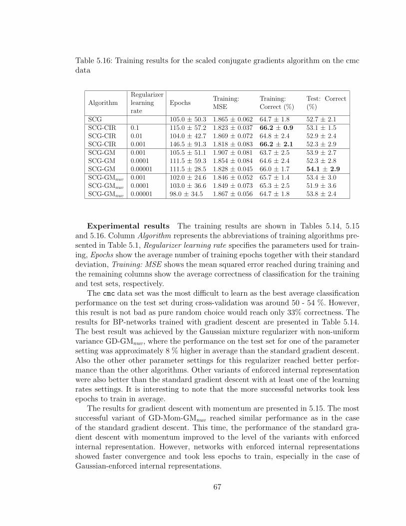
Table 5.16: Training results for the scaled conjugate gradients algorithm on the cmcdata

AlgorithmRegularizerlearningrate

EpochsTraining:MSE

Training:Correct (%)

Test: Correct(%)

SCG 105.0 ± 50.3 1.865 ± 0.062 64.7 ± 1.8 52.7 ± 2.1

SCG-CIR 0.1 115.0 ± 57.2 1.823 ± 0.037 66.2 ± 0.9 53.1 ± 1.5SCG-CIR 0.01 104.0 ± 42.7 1.869 ± 0.072 64.8 ± 2.4 52.9 ± 2.4SCG-CIR 0.001 146.5 ± 91.3 1.818 ± 0.083 66.2 ± 2.1 52.3 ± 2.9

SCG-GM 0.001 105.5 ± 51.1 1.907 ± 0.081 63.7 ± 2.5 53.9 ± 2.7SCG-GM 0.0001 111.5 ± 59.3 1.854 ± 0.084 64.6 ± 2.4 52.3 ± 2.8SCG-GM 0.00001 111.5 ± 28.5 1.828 ± 0.045 66.0 ± 1.7 54.1 ± 2.9

SCG-GMnuv 0.001 102.0 ± 24.6 1.846 ± 0.052 65.7 ± 1.4 53.4 ± 3.0SCG-GMnuv 0.0001 103.0 ± 36.6 1.849 ± 0.073 65.3 ± 2.5 51.9 ± 3.6SCG-GMnuv 0.00001 98.0 ± 34.5 1.867 ± 0.056 64.7 ± 1.8 53.8 ± 2.4

Experimental results The training results are shown in Tables 5.14, 5.15and 5.16. Column Algorithm represents the abbreviations of training algorithms pre-sented in Table 5.1, Regularizer learning rate specifies the parameters used for train-ing, Epochs show the average number of training epochs together with their standarddeviation, Training: MSE shows the mean squared error reached during training andthe remaining columns show the average correctness of classification for the trainingand test sets, respectively.

The cmc data set was the most difficult to learn as the best average classificationperformance on the test set during cross-validation was around 50 - 54 %. However,this result is not bad as pure random choice would reach only 33% correctness. Theresults for BP-networks trained with gradient descent are presented in Table 5.14.The best result was achieved by the Gaussian mixture regularizer with non-uniformvariance GD-GMnuv, where the performance on the test set for one of the parametersetting was approximately 8 % higher in average than the standard gradient descent.Also the other other parameter settings for this regularizer reached better perfor-mance than the other algorithms. Other variants of enforced internal representationwere also better than the standard gradient descent with at least one of the learningrates settings. It is interesting to note that the more successful networks took lessepochs to train in average.

The results for gradient descent with momentum are presented in 5.15. The mostsuccessful variant of GD-Mom-GMnuv reached similar performance as in the caseof the standard gradient descent. This time, the performance of the standard gra-dient descent with momentum improved to the level of the variants with enforcedinternal representation. However, networks with enforced internal representationsshowed faster convergence and took less epochs to train, especially in the case ofGaussian-enforced internal representations.

67

40

45

50

55

60

0.00

05

0.00

07

0.00

09

0.00

1

0.00

11

0.00

13

0.00

15

Regularizer learning rate

Cor

rect

ness

(%

)

GD−GIRnuv

40

45

50

55

60

5e−

005

7e−

005

9e−

005

0.00

01

0.00

011

0.00

013

0.00

015

Regularizer learning rate

Cor

rect

ness

(%

)

GD−Mom−GIRnuv

40

45

50

55

605e

−00

6

7e−

006

9e−

006

1e−

005

1.1e

−00

5

1.3e

−00

5

1.5e

−00

5Regularizer learning rate

Cor

rect

ness

(%

)

SCG−GIR

Figure 5.15: Robustness of the GD-GMnuv, GD-Mom-GMnuv and SCG-GM algo-rithms with respect to their learning rates on the cmc data set.

Scaled conjugate gradients 5.16 showed overall the best performance. The bestperforming algorithm was SCG-GM with average correctness around 54 % for two ofthe learning rates, followed by SCG-GMnuv. The number of epochs needed to trainthe networks was approximately the same for all the tested algorithms.

Overall, the best results were achieved with GMnuv and GM regularizers. To testthe robustness of these algorithms with respect to values of their regularizer learningrates, additional cross-validation tests were made for the best performing algorithms,namely for GD-GMnuv with αGM = 0.001, GD-Mom-GMnuv with αGM = 0.0001 andfor SCG-GM with αGM = 0.00001. Each of the learning rates was altered by 10 to 50% and used in cross-validation. The results are presented in Figure 5.15 in the formof boxplots. The SCG-GM algorithm showed the most consistent performance acrossall cases. On the other hand, GD-Mom-GMnuv had the most varying performance.

Analysis of internal representations Similarly as with the iris data set,we shall analyse the internal representations formed during training . The internalrepresentations formed in the standard gradient descent (GD) and in the gradientdescent with internal representations enforced by the mixture of Gaussians with

68

0 2 4 6 8 10−1

0

1

2

3

4

5

6

7

8

SOM Neighbor Weight Distances

Figure 5.16: Neighbour distances in the 10 × 10 self-organizing map trained on a setof internal representations of a BP-network trained by standard gradient descent onthe cmc data set.

non-uniform variance (GD-GMnuv) were compared. These two algorithms were againselected because they showed the largest difference in performance in cross-validation,over 8 % (Table 5.14) for αGM = 0.001. One network trained by each of the twoalgorithm was selected for the analysis, the network was trained on the same set oftraining patterns during the cross-validation to ensure comparability of the results.The internal representations formed during the cross-validation were extracted forboth algorithms.

The internal representations were used as input patterns for a self-organizing map(SOM) with 10 × 10 units in hexagonal topology. Figures 5.16 and 5.18 show the dis-tances between neighbouring units for one networks trained by GD and GD-GMnuv

respectively. Figures 5.17 and 5.19 show the mappings of internal representation ontothe units in the trained SOM with respect to their corresponding target class. Thecolour of the units corresponds to the class attribute, i.e. the choice of contraceptivemethod. Red colour represents no-use, blue colour corresponds to long-term contra-ceptive methods and green colour to short-term methods. When different classes aremapped onto the same unit with equal proportions, the unit has grey colour.

The neighbour distances for the gradient descent algorithm GD (Figure 5.16)show a few regions of close units and a few regions with larger distance from theneighbouring units. When we look at the mappings produced by the self-organizingmap, we can see that the clusters formed in the SOM do not correspond to the targetclasses, as they did for the iris data set 5.12. Only the red units (no-use) are partiallyclustered together in the lower part of the SOM, which signifies that they form similarinternal representations. This also positively affects the performance of the network

69

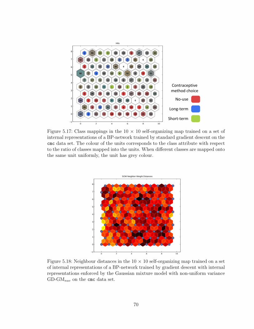
0 2 4 6 8 10−1

0

1

2

3

4

5

6

7

8

44 2 21 4 10 15 16 18 29 11

35 5 6 31 3 4 10 1 4 25

33 1 13 7 9 28 10 0 17 6

1 26 4 10 13 1 27 20 22 13

8 2 12 9 1 13 2 4 25 19

7 17 5 4 18 6 27 6 4 21

92 7 1 12 11 6 52 6 2 51

1 12 6 8 40 0 13 24 23 13

42 15 5 2 19 3 7 21 0 15

1 55 23 9 10 10 6 47 8 30

Hits

No-use

Long-term

Short-term

Contraceptive method choice

Figure 5.17: Class mappings in the 10 × 10 self-organizing map trained on a set ofinternal representations of a BP-network trained by standard gradient descent on thecmc data set. The colour of the units corresponds to the class attribute with respectto the ratio of classes mapped into the units. When different classes are mapped ontothe same unit uniformly, the unit has grey colour.

0 2 4 6 8 10−1

0

1

2

3

4

5

6

7

8

SOM Neighbor Weight Distances

Figure 5.18: Neighbour distances in the 10 × 10 self-organizing map trained on a setof internal representations of a BP-network trained by gradient descent with internalrepresentations enforced by the Gaussian mixture model with non-uniform varianceGD-GMnuv on the cmc data set.

70

0 2 4 6 8 10−1

0

1

2

3

4

5

6

7

8

22 33 8 19 7 7 9 15 23 13

16 21 14 12 8 11 18 12 13 29

22 7 13 13 17 20 15 8 9 28

28 9 7 13 21 5 12 10 3 35

10 1 18 8 12 5 10 10 35 12

28 10 9 7 19 13 8 8 16 30

13 5 23 17 16 6 12 23 15 8

18 9 19 21 19 12 10 9 27 12

7 4 15 15 7 21 15 13 18 12

27 23 15 24 20 18 8 22 5 16

Hits

No-use

Long-term

Short-term

Contraceptive method choice

Figure 5.19: Class mappings in the 10 × 10 self-organizing map trained on a set ofinternal representations of a BP-network trained by gradient descent with internalrepresentations enforced by the Gaussian mixture model with non-uniform varianceGD-GMnuv on the cmc data set. The colour of the units corresponds to the classattribute with respect to the ratio of classes mapped into the units. When differentclasses are mapped onto the same unit uniformly, the unit has grey colour.

with respect to this particular class. If we modify the cmc classification task to asimpler problem of distinguishing no-use versus use of some method (regardless ofthe type, long-term and short-term), the networks trained by GD reach 65,03 %correctness. On the other hand, when the networks have to distinguish either of theother two contraceptive methods from the rest, the performance stays around 50 %.

The gradient descent with internal representations enforced by the Gaussian mix-ture model with non-uniform variance GD-GMnuv showed significantly better per-formance 5.14. The neighbour distances for this algorithm are displayed in Figure5.18. Overall, there are no large regions of close units. Most of the units are farfrom their neighbours compared to the distances for the GD algorithm 5.16. Thissituation indicates that the GD-GMnuv algorithm formed a large number of smallclusters of internal representations. This is confirmed by the next Figure 5.19, wherethe numbers of internal representations mapped onto each unit are well distributedover the whole map. The red units are mostly grouped together, similarly to theprevious case. Also the performance in distinguishing the class of ’no-use’ from theother classes reached 67,21 % correctness. In this case, also the green units (short-term) are clustered together and separated from the grey units. When the task is toclassify the short-term contraceptive methods versus the rest, the correctness reaches65.7 % whereas GD achieved only 50.1 % correctness. Therefore well-formed clustersof similar internal representations help to improve the accuracy of classification. Onthe other hand, difficult tasks demand larger number of different clusters of internal

71

representations.

5.2.3 Pima Indians Diabetes Data Set

Table 5.17: Description of the Pima Indians Diabetes Data Set

Attribute Type Description

Number of times pregnant numericalPlasma glucose concentration numericalafter 2 hours in an oralglucose tolerance testDiastolic blood pressure numerical mmHgTriceps skin fold thickness numerical mm2-Hour serum insulin numerical mU/mlBody mass index numerical weight in kg/(height in m)2

Diabetes pedigree function numericalAge (years) numericalClass variable binary 1 = tested positive

class attribute for diabetes

The Pima Indians Diabetes 3 data set is a subset of a medical survey on popula-tion of Pima Indian origin. The prevalence of diabetes was studied on female patientsliving near Phoenix, Arizona. The data set contains eight attributes and one targetclass which shows whether the patient suffered from diabetes. A more detailed de-scription of the attributes is displayed in Table 5.17. The data set consists of 768patterns and contains no missing values. Out of the 768 patterns there are 268 casesof positive tests for diabetes and 500 negative cases.

The numerical attributes were again normalized to zero mean and unit standarddeviation. The target class was transformed to bipolar 1-of-c encoding for c = 2.Therefore, the data set used for training consisted of 8 numerical inputs and 2 targetfeatures. Again, the tested algorithms are listed in Table 5.1, values of the learningrate αGD = 0.1 and momentum rate αMom = 0.1 were experimentally optimized.Architectures with 5 to 25 hidden neurons with hyperbolic tangent were tested, thebest results were achieved for BP-networks with 10 hidden units.

Experimental results The training results are shown in Tables 5.18, 5.19and 5.20. Column Algorithm represents the abbreviations of training algorithms pre-sented in Table 5.1, Regularizer learning rate specifies the parameters used for train-ing, Epochs show the average number of training epochs together with their standard

3http://archive.ics.uci.edu/ml/datasets/Pima+Indians+Diabetes

72

Table 5.18: Training results for the gradient descent algorithm on the pima data set.

AlgorithmRegularizerlearningrate

EpochsTraining:MSE

Training:Correct (%)

Test: Correct(%)

GD 399.0 ± 265.9 1.315 ± 0.197 80.3 ± 4.4 75.1 ± 7.5

GD-CIR 0.1 1618.5 ± 895.0 1.542 ± 0.108 77.7 ± 2.9 74.6 ± 5.6GD-CIR 0.01 1204.5 ± 1554.1 1.380 ± 0.056 76.9 ± 2.3 74.1 ± 5.6GD-CIR 0.001 441.5 ± 200.7 1.361 ± 0.121 79.0 ± 3.0 73.6 ± 4.8

GD-GM 0.001 161.5 ± 101.6 1.427 ± 0.121 79.4 ± 2.4 77.7 ± 6.1GD-GM 0.0001 222.0 ± 106.5 1.296 ± 0.264 80.8 ± 5.2 75.3 ± 6.4GD-GM 0.00001 256.0 ± 169.9 1.352 ± 0.157 79.6 ± 3.6 75.4 ± 7.2

GD-GMnuv 0.001 429.0 ± 181.5 1.345 ± 0.198 81.4 ± 3.5 74.9 ± 5.9GD-GMnuv 0.0001 281.0 ± 134.2 1.289 ± 0.162 81.4 ± 3.5 73.7 ± 8.6GD-GMnuv 0.00001 223.0 ± 137.7 1.391 ± 0.178 79.2 ± 3.5 75.5 ± 6.7

Table 5.19: Training results for the gradient descent algorithm with momentum onthe pima data set.

AlgorithmRegularizerlearningrate

EpochsTraining:MSE

Training:Correct (%)

Test: Correct(%)

GD-Mom 410.5 ± 186.8 1.380 ± 0.171 80.0 ± 3.4 74.6 ± 8.4

GD-Mom-CIR 0.1 1500.0 ± 1312.8 1.580 ± 0.153 78.3 ± 3.0 76.2 ± 6.9GD-Mom-CIR 0.01 2762.0 ± 1913.3 1.374 ± 0.086 76.4 ± 2.2 73.2 ± 5.4GD-Mom-CIR 0.001 568.0 ± 628.1 1.415 ± 0.145 79.1 ± 2.7 73.4 ± 6.0

GD-Mom-GM 0.001 193.0 ± 96.2 1.382 ± 0.137 80.8 ± 2.4 73.7 ± 8.3GD-Mom-GM 0.0001 175.0 ± 133.4 1.436 ± 0.098 79.5 ± 2.1 75.9 ± 6.4GD-Mom-GM 0.00001 201.5 ± 158.0 1.396 ± 0.132 79.7 ± 2.6 73.7 ± 7.2

GD-Mom-GMnuv 0.001 494.5 ± 537.2 1.361 ± 0.131 81.5 ± 2.1 75.2 ± 6.7GD-Mom-GMnuv 0.0001 293.5 ± 225.6 1.295 ± 0.253 81.8 ± 4.6 74.9 ± 7.6GD-Mom-GMnuv 0.00001 200.0 ± 125.1 1.390 ± 0.201 79.7 ± 4.1 72.9 ± 7.8

deviation, Training: MSE shows the mean squared error reached during training andthe remaining columns show the average correctness of classification for the trainingand test sets, respectively.

In training with gradient descent algorithm (Table5.18), the best performingnetworks were trained with internal representations enforced by the Gaussian mixturemodel with uniform variance GD-GM. Their results were better than the standardgradient descent for all the displayed values of the regularizer learning rates, in oneof the cases the result was 2.6 % better. Other variants of the algorithm performedworse or the same as the standard variant.

The results for gradient descent with momentum are displayed in Table 5.19 . In

73

Table 5.20: Training results for the scaled conjugate gradients algorithm on the pimadata

AlgorithmRegularizerlearningrate

EpochsTraining:MSE

Training:Correct (%)

Test: Correct(%)

SCG 77.0 ± 39.1 0.758 ± 0.109 89.2 ± 2.5 72.1 ± 6.9

SCG-CIR 0.1 89.0 ± 5.7 1.199 ± 0.056 78.4 ± 1.5 76.0 ± 7.7SCG-CIR 0.01 82.5 ± 45.1 0.824 ± 0.146 87.3 ± 3.5 73.3 ± 5.3SCG-CIR 0.001 65.0 ± 39.1 0.815 ± 0.124 88.2 ± 3.0 71.6 ± 4.6

SCG-GM 0.001 89.5 ± 118.3 0.871 ± 0.170 86.4 ± 3.7 70.1 ± 5.4SCG-GM 0.0001 64.5 ± 31.5 0.807 ± 0.171 87.9 ± 3.4 73.7 ± 6.3SCG-GM 0.00001 63.0 ± 38.0 0.831 ± 0.152 87.7 ± 3.4 73.8 ± 6.4

SCG-GMnuv 0.001 53.5 ± 14.9 0.856 ± 0.080 87.1 ± 2.0 72.0 ± 7.2SCG-GMnuv 0.0001 66.0 ± 47.3 0.830 ± 0.133 87.7 ± 2.8 71.4 ± 7.4SCG-GMnuv 0.00001 83.5 ± 77.5 0.812 ± 0.159 88.0 ± 3.3 72.0 ± 6.6

this case, the best performance was achieved by networks trained with GD-Mom-CIR, where the internal representations were enforced by the polynomial objectivefunction (Section4.6.1). On the other hand, the number of epochs needed to trainthese networks was almost three times higher than for the standard gradient descentwith momentum. Other variants of enforced internal representations also performedbetter than the standard algorithm in most of cases.

Finally, the results for scaled conjugate gradients are presented in Table 5.20.Again, CIR regularizer had the best performance on the test set. The results showa clear tendency of SCG algorithm to overfit, as the performance on the test setdeteriorated significantly compared to the performance on the training set. The onlyexception is the SCG-CIR with learning rate αCIR = 0.1 where the regularizer pre-vented overfitting and the correctness on the training and test set remained almostthe same.

Overall, the best results were achieved with enforced internal representations,either with GM or CIR regularizers. To test the robustness of these algorithms withrespect to values of their regularizer learning rates, additional cross-validation testswere made for the best performing algorithms, namely for GD-GM with αGM =0.001, GD-Mom-CIR with αCIR = 0.1 and for SCG-CIR with αCIR = 1.0. Each ofthe learning rates was altered by 10% to 50 % and used in cross-validation. Theresults are presented in Figrue 5.20 in the form of boxplots. The consistency of thealgorithms varies quite significantly, especially in the case of GD-Mom-CIR, wherethe correctness ranges from 60 % to 90 %.

Analysis of internal representations Standard scaled conjugate gradientsSCG and scaled conjugate gradients with polynomial-enforced internal representa-tions SCG-CIR showed the largest difference in performance on the pima data set.

74

50

60

70

80

90

100

0.00

05

0.00

07

0.00

09

0.00

1

0.00

11

0.00

13

0.00

15

Regularizer learning rate

Cor

rect

ness

(%

)

GD−GIR

50

60

70

80

90

100

0.05

0.07

0.09

0.1

0.11

0.13

0.15

Regularizer learning rate

Cor

rect

ness

(%

)

GD−Mom−CIR

50

60

70

80

90

100

0.5

0.7

0.9

1 1.1

1.3

1.5

Regularizer learning rate

Cor

rect

ness

(%

)SCG−CIR

Figure 5.20: Robustness of the GD-GM, GD-Mom-CIR and SCG-CIR algorithmswith respect to their learning rates on the pima data set.

The correctness of SCG-CIR for αCIR = 0.1 was 4 % higher than the SCG. There-fore these two algorithms were selected for the analysis of internal representations,which they form during training. Self-organizing map with 7 × 7 units in hexagonaltopology was trained on the internal representations of a network trained by bothalgorithms.

The distances between neighbouring units trained on the internal representationsfrom a network trained by SCG are shown in Figure 5.21. There are two clearlyformed clusters of units with small distances between them. Figure 5.22 shows themapping of internal representations with respect to their target class. Green colourcorresponds to negative result of diabetes test and red colour to positive test. Fromthis figure, we can see that the two well-formed clusters in 5.21 both correspond tothe same target class, i. e. negative test for diabetes. The red units are mostly greyishas the internal representations mapped into them do not belong all to the same class.Therefore we can suppose that the network may have problems with identifying thepositive tests.

The results of the self-organizing map trained on the internal representationsproduced by the SCG-CIR algorithm are displayed in Figures 5.23 and 5.24. The

75

−1 0 1 2 3 4 5 6 7−1

0

1

2

3

4

5

6

SOM Neighbor Weight Distances

Figure 5.21: Neighbour distances in the 10 × 10 self-organizing map trained on aset of internal representations of a BP-network trained by standard scaled conjugategradients on the pima data set.

distances between units in the trained SOM in 5.23 show three clusters. By lookingon the next figure 5.24, two of the clusters correspond again to the negative diabetestest (the clusters in the lower part of the map). On the other hand, the cluster inthe top left corner of the map corresponds mostly to the red units - positive diabetestest. Also the other red units are better separated from the green units. This maybe the reason of the better performance of SCG-CIR.

76

−1 0 1 2 3 4 5 6 7−1

0

1

2

3

4

5

6

29 9 12 19 19 14 9

19 23 16 10 15 18 14

35 9 13 10 10 22 12

15 12 10 11 16 15 21

11 14 13 11 13 17 38

26 19 8 10 15 6 39

22 5 7 13 7 24 13

Hits

Positive

Negative

Diabetes test

Figure 5.22: Class mappings in the 10 × 10 self-organizing map trained on a setof internal representations of a BP-network trained by standard scaled conjugategradients on the pima data set. The colour of the units corresponds to the classattribute with respect to the ratio of classes mapped into the units. When differentclasses are mapped onto the same unit uniformly, the unit has grey colour.

−1 0 1 2 3 4 5 6 7−1

0

1

2

3

4

5

6

SOM Neighbor Weight Distances

Figure 5.23: Neighbour distances in the 10 × 10 self-organizing map trained on aset of internal representations of a BP-network trained by scaled conjugate gradientswith internal representations enforced by the polynomial regularizer SCG-CIR onthe pima data set.

77

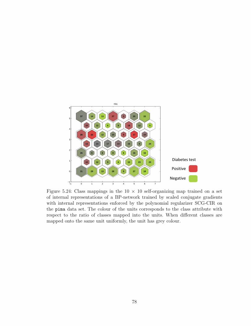
−1 0 1 2 3 4 5 6 7−1

0

1

2

3

4

5

6

31 29 13 28 9 27 18

10 12 9 6 15 23 23

26 5 6 8 6 16 16

13 14 17 14 16 8 24

26 23 12 10 9 17 10

10 12 6 9 18 12 5

37 14 13 27 3 20 33

Hits

Positive

Negative

Diabetes test

Figure 5.24: Class mappings in the 10 × 10 self-organizing map trained on a setof internal representations of a BP-network trained by scaled conjugate gradientswith internal representations enforced by the polynomial regularizer SCG-CIR onthe pima data set. The colour of the units corresponds to the class attribute withrespect to the ratio of classes mapped into the units. When different classes aremapped onto the same unit uniformly, the unit has grey colour.

78

5.3 World Development Indicators

For additional evaluation of the discussed algorithms on a real-world example, WorldDevelopment Indicators (WDI) issued annually by the World Bank. The World De-velopment Indicators comprise of various indicators which are used to measure theprogress of development of countries. Each year, a set of more than 800 indicators inaverage is published for world economies 4. For our experiments, the data from years1999-2008 were used. The indicators were used to construct a task of estimating thegross domestic product from the values of indicators selected during preprocessing.

5.3.1 Preprocessing

The original dataset comprised of 869 indicators for 209 countries. However, the WDIdata are very sparse as some indicators are difficult to obtain especially from devel-oping countries and from countries with unstable political situation. Some indicatorsare also not assessed every year (e.g. data from national censuses). Therefore somemethod for dealing with missing values had to be employed.

Missing values As a first step, some of the indicators and countries with ex-cessively large number of missing values have to be excluded from further processing.The indicators where the number of missing values exceeded 40% across all countriesand years were removed. This left approximately 70% of the indicators. The coun-tries with more than 40% of missing values across all indicators and years were alsodiscarded. After this procedure approximately 83% of the countries remained.

The published indicators are given in various units, e.g. US dollar, percentage oras indices without units. Some indicators are given also in the local currency unit(LCU). These values are not directly comparable between countries and thereforethey were removed. After this removal, 173 countries and 384 indicators were left forfurther processing.

Next, a method for completion (imputation) of missing data was used. Thereare many methods developed for imputation of missing values. Some methods weredeveloped specifically for cross-sectional time series data, such as the World Devel-opment Indicators, see Honaker and King [17]. Their method relies on creating aprobabilistic generative model for the data. Unfortunately, it yields reliable resultsonly for data with small number of missing values or for sufficiently large datasets.Therefore a method suitable for imputation on smaller and sparser datasets had tobe used.

Data imputation by clustering has proven to be useful in many large-dimensionalapplications, such as in bioinformatics, see [16], [?]. For imputation of the WDI data,the 1-nearest neighbour method (1-nn) was used. This method replaces the missingvalues for a given country and a given indicator by the values of the same indicator

4http://data.worldbank.org/indicator

79

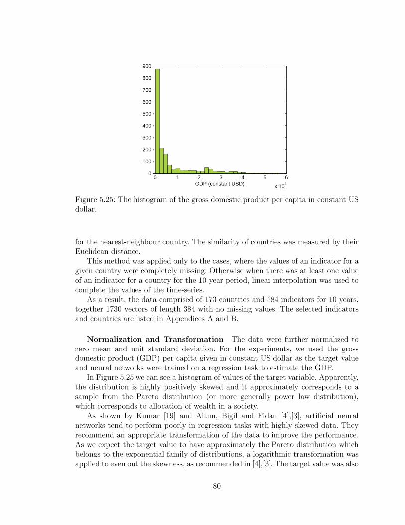
0 1 2 3 4 5 6

x 104

0

100

200

300

400

500

600

700

800

900

GDP (constant USD)

Figure 5.25: The histogram of the gross domestic product per capita in constant USdollar.

for the nearest-neighbour country. The similarity of countries was measured by theirEuclidean distance.

This method was applied only to the cases, where the values of an indicator for agiven country were completely missing. Otherwise when there was at least one valueof an indicator for a country for the 10-year period, linear interpolation was used tocomplete the values of the time-series.

As a result, the data comprised of 173 countries and 384 indicators for 10 years,together 1730 vectors of length 384 with no missing values. The selected indicatorsand countries are listed in Appendices A and B.

Normalization and Transformation The data were further normalized tozero mean and unit standard deviation. For the experiments, we used the grossdomestic product (GDP) per capita given in constant US dollar as the target valueand neural networks were trained on a regression task to estimate the GDP.

In Figure 5.25 we can see a histogram of values of the target variable. Apparently,the distribution is highly positively skewed and it approximately corresponds to asample from the Pareto distribution (or more generally power law distribution),which corresponds to allocation of wealth in a society.

As shown by Kumar [19] and Altun, Bigil and Fidan [4],[3], artificial neuralnetworks tend to perform poorly in regression tasks with highly skewed data. Theyrecommend an appropriate transformation of the data to improve the performance.As we expect the target value to have approximately the Pareto distribution whichbelongs to the exponential family of distributions, a logarithmic transformation wasapplied to even out the skewness, as recommended in [4],[3]. The target value was also

80

−1 −0.5 0 0.5 10

20

40

60

80

100

120

140

160

GDP

Figure 5.26: The histogram of the gross domestic product per capita in constant USdollar after the logarithmic transformation and normalization to zero mean and unitstandard deviation.

transformed by a sigmoid function to move the values further from the borders of theoutput interval [−1, 1]. The histogram of the GDP values after the transformationand normalization is shown in Figure ??.

5.3.2 Experimental results

Unlike the previously presented training tasks, the task of estimating the gross do-mestic product from the World Development Indicators is a regression task. Similarlyto the previous data sets, the algorithms listed in Table 5.1 were tested on this taskwith various parameter settings. The learning rates of gradient descent αGD andmomentum rates αMom were optimized experimentally and the values, which exhib-ited the best results were used as the baseline for further experiments with enforcedinternal representations. The optimized parameters were set to the following values:αGD = 0.1 and αMom = 0.05.

The values of learning rates for the regularizers CIR, GM and GMnuv were op-timized experimentally in the following way: the initial value was set to 1.0 anddecreased by a factor of 10 until the performance stopped improving. For each of theregularizers, the results are presented for two values of parameters which yielded thebest results.

Several architectures of BP-networks with one hidden layer were tested, with384 input neurons, 1 output neuron and 5 to 50 hidden neurons. The results whichare presented further cover the networks with 10 hidden units, as the performancestayed mostly the same even with more hidden neurons. Only the larger networks

81

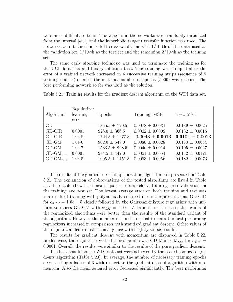
were more difficult to train. The weights in the networks were randomly initializedfrom the interval [-1,1] and the hyperbolic tangent transfer function was used. Thenetworks were trained in 10-fold cross-validation with 1/10-th of the data used asthe validation set, 1/10-th as the test set and the remaining 2/10-th as the trainingset.

The same early stopping technique was used to terminate the training as forthe UCI data sets and binary addition task. The training was stopped after theerror of a trained network increased in 6 successive training strips (sequence of 5training epochs) or after the maximal number of epochs (5000) was reached. Thebest performing network so far was used as the solution.

Table 5.21: Training results for the gradient descent algorithm on the WDI data set.

AlgorithmRegularizerlearningrate

Epochs Training: MSE Test: MSE

GD 1365.5 ± 720.5 0.0078 ± 0.0031 0.0139 ± 0.0025GD-CIR 0.0001 928.0 ± 366.5 0.0062 ± 0.0009 0.0132 ± 0.0016GD-CIR 1.0e-5 1724.5 ± 1277.8 0.0043 ± 0.0013 0.0104 ± 0.0013GD-GM 1.0e-6 902.0 ± 547.0 0.0086 ± 0.0028 0.0133 ± 0.0034GD-GM 1.0e-7 1533.5 ± 998.5 0.0046 ± 0.0014 0.0105 ± 0.0027GD-GMnuv 0.0001 984.5 ± 442.0 0.0061 ± 0.0054 0.0112 ± 0.0121GD-GMnuv 1.0e-5 1005.5 ± 1451.3 0.0063 ± 0.0056 0.0182 ± 0.0073

The results of the gradient descent optimization algorithm are presented in Table5.21. The explanation of abbreviations of the tested algorithms are listed in Table5.1. The table shows the mean squared errors achieved during cross-validation onthe training and test set. The lowest average error on both training and test setsis a result of training with polynomially enforced internal representations GD-CIRfor αCIR = 1.0e − 5 closely followed by the Gaussian-mixture regularizer with uni-form variances GD-GM with αGM = 1.0e − 7. In most of the cases, the results ofthe regularized algorithms were better than the results of the standard variant ofthe algorithm. However, the number of epochs needed to train the best-performingregularizers increased in comparison with standard gradient descent. Other values ofthe regularizers led to faster convergence with slightly worse results.

The results for gradient descent with momentum are displayed in Table 5.22.In this case, the regularizer with the best results was GD-Mom-GMnuv for αGM =0.0001. Overall, the results were similar to the results of the pure gradient descent.

The best results on the WDI data set were achieved by the scaled conjugate gra-dients algorithm (Table 5.23). In average, the number of necessary training epochsdecreased by a factor of 3 with respect to the gradient descent algorithm with mo-mentum. Also the mean squared error decreased significantly. The best performing

82

Table 5.22: Training results for gradient descent with momentum on the WDI dataset.

AlgorithmRegularizerlearningrate

Epochs Training: MSE Test: MSE

GD-Mom 1387.5 ± 829.4 0.0044 ± 0.0018 0.0110 ± 0.0020GD-Mom-CIR 0.0001 1152.5 ± 677.6 0.0060 ± 0.0027 0.0130 ± 0.0027GD-Mom-CIR 1.0e-5 1383.0 ± 1008.3 0.0046 ± 0.0016 0.0113 ± 0.0020GD-Mom-GM 1.0e-6 1480.0 ± 700.6 0.0071 ± 0.0011 0.0119 ± 0.0019GD-Mom-GM 1.0e-7 1341.5 ± 1046.2 0.0054 ± 0.0032 0.0109 ± 0.0026GD-Mom-GMnuv 0.0001 1388.0 ± 620.2 0.0043 ± 0.0002 0.0077 ± 0.0027GD-Mom-GMnuv 1.0e-5 1113.5 ± 1340.7 0.0047 ± 0.0036 0.0160 ± 0.0069

regularizers were SCG-CIR with αCIR = 0.001 and SCG-GM with αGM = 1.0e− 5.However, the regularizers did not bring a significant improvement compared to stan-dard SCG.

Table 5.23: Training results for the scaled conjugate gradients algorithm on the WDIdata set.

AlgorithmRegularizerlearningrate

Epochs Training: MSE Test: MSE

SCG 340.0 ± 104.4 0.0029 ± 0.0007 0.0067 ± 0.0010SCG-CIR 0.01 495.0 ± 485.1 0.0034 ± 0.0009 0.0079 ± 0.0010SCG-CIR 0.001 409.0 ± 141.5 0.0025 ± 0.0006 0.0063 ± 0.0009SCG-GM 0.0001 367.0 ± 146.0 0.0057 ± 0.0011 0.0093 ± 0.0019SCG-GM 1.0e-5 464.0 ± 215.2 0.0026 ± 0.0013 0.0063 ± 0.0019SCG-GMnuv 0.001 1905.6 ± 2227.8 0.0055 ± 0.0052 0.0142 ± 0.0037SCG-GMnuv 0.0001 288.0 ± 90.9 0.0025 ± 0.0012 0.0067 ± 0.0013

Analysis of formed internal representations Similarly to the previoustasks, we shall analyze the formed internal representations in the networks trained bythe discussed algorithms. To better visualize the distribution of internal representa-tions with respect to the data set, a class was assigned to each internal representationdepending on the income group of the country corresponding to the network’s in-put. The income groups are a part of classification of world countries used by WorldBank. The income groups consist of the following categories:

83

• High income: OECD (28 countries in the data set)

• High income: nonOECD (19 countries in the data set)

• Low income (36 countries in the data set)

• Lower middle income (49 countries in the data set)

• Upper middle income (41 countries in the data set).

Self-organizing maps (SOM) were trained on internal representations formed bygradient descent (GD) and scaled conjugate gradients (SCG) with and without thepresented regularizers. The maps had 7 × 7 units organized in hexagonal topology.

Figure 5.27 shows the SOM trained on internal representations of one of thenetworks trained by gradient descent. Figure 5.27a shows the distances betweenneighbouring units. Lighter colours correspond to smaller distances, darker coloursto larger distances. There are several clusters of closely adjacent units in the leftand right parts of the map. The next figure 5.27b shows the mapping of internalrepresentations into the individual units in the map. The colours of units correspondto the class of majority of internal representations mapped into it, the more greyishthe colour of unit is, the less the unit is class specific. The size of the coloured regionin each unit represents the fraction of internal representations which was mappedinto it.

The clusters formed in 5.27a correspond nicely to the groups in 5.27b. The clusterin the top left corner groups together the internal representations of high incomeOECD countries (mixed with high income nonOECD countries) whereas the clusteron the right side of the figure groupes the low income countries. Other groups areless well-defined.

Similar trends can be seen in Figures 5.28 and 5.29 for the networks trainedwith CIR and GMnuv regularizers. Again, the high income OECD countries and thelow income countries are mostly grouped together and on the opposite sides of thetrained SOMs. The maps are very similar to each other which may be caused bysimilar quality of the training results (Table ??). No algorithm showed significantlydifferent performance.

The SOMs corresponding to the networks trained by scaled conjugate gradients5.30, 5.31 and ?? show again similar trends. Two main clusters are formed in thenetwork, one corresponds to the high income countries and the second to the lowincome countries. The other income groups do not form any clear clusters and theyare scattered between the two main groups. However, the internal representationsformed by scaled conjugate gradients are less diverse than the representations formedby gradient descent, i. e. almost all representations which belong to high income orlow income groups are mapped into the same units in the map. Also the otherincome groups are separated better than in the case of gradient descent, althoughtheir borders are mostly blurred together. The performance of both the regularizersSCG-CIR an SCG-GMnuv yielded very similar results as the standard variant of the

84

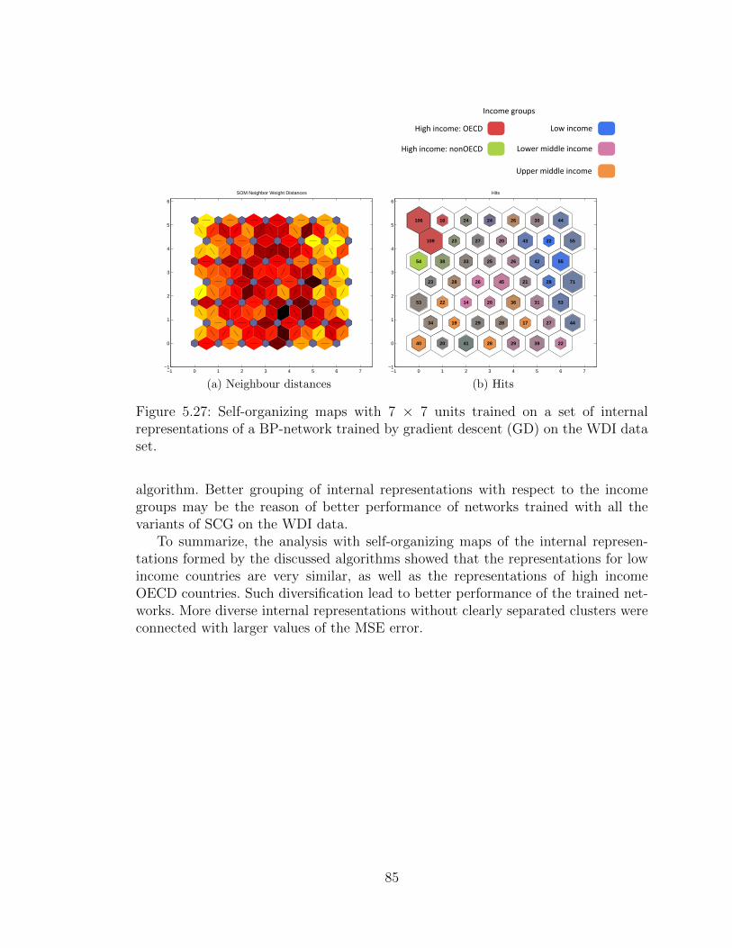
Income groups

High income: OECD

High income: nonOECD

Low income

Lower middle income

Upper middle income

−1 0 1 2 3 4 5 6 7−1

0

1

2

3

4

5

6

SOM Neighbor Weight Distances

(a) Neighbour distances

−1 0 1 2 3 4 5 6 7−1

0

1

2

3

4

5

6

40 20 41 28 29 39 22

34 19 29 28 17 27 44

53 22 14 20 36 31 53

23 28 26 45 21 28 71

54 38 33 25 26 42 55

109 23 27 20 43 22 55

106 16 24 24 26 30 44

Hits

(b) Hits

Figure 5.27: Self-organizing maps with 7 × 7 units trained on a set of internalrepresentations of a BP-network trained by gradient descent (GD) on the WDI dataset.

algorithm. Better grouping of internal representations with respect to the incomegroups may be the reason of better performance of networks trained with all thevariants of SCG on the WDI data.

To summarize, the analysis with self-organizing maps of the internal represen-tations formed by the discussed algorithms showed that the representations for lowincome countries are very similar, as well as the representations of high incomeOECD countries. Such diversification lead to better performance of the trained net-works. More diverse internal representations without clearly separated clusters wereconnected with larger values of the MSE error.

85

Income groups

High income: OECD

High income: nonOECD

Low income

Lower middle income

Upper middle income

−1 0 1 2 3 4 5 6 7−1

0

1

2

3

4

5

6

SOM Neighbor Weight Distances

(a) Neighbour distances

−1 0 1 2 3 4 5 6 7−1

0

1

2

3

4

5

6

84 31 56 34 43 35 28

59 27 21 30 29 39 56

43 27 29 19 36 24 54

18 13 16 14 22 15 48

48 14 20 27 26 32 47

38 48 33 10 36 24 39

90 23 12 32 44 70 67

Hits

(b) Hits

Figure 5.28: Self-organizing maps with 7 × 7 units trained on a set of internal rep-resentations of a BP-network trained by gradient descent with polynomial-enforcedinternal representations (GD-CIR) on the WDI data set.

Income groups

High income: OECD

High income: nonOECD

Low income

Lower middle income

Upper middle income

−1 0 1 2 3 4 5 6 7−1

0

1

2

3

4

5

6

SOM Neighbor Weight Distances

(a) Neighbour distances

−1 0 1 2 3 4 5 6 7−1

0

1

2

3

4

5

6

51 28 50 27 45 46 49

35 44 54 34 42 37 39

47 25 14 26 17 28 24

30 38 32 23 42 24 56

35 33 11 30 38 37 36

34 30 33 30 28 40 49

43 21 46 50 34 27 38

Hits

(b) Hits

Figure 5.29: Self-organizing maps with 7 × 7 units trained on a set of internal repre-sentations of a BP-network trained by gradient descent with internal representationsenforced by the Gaussian mixture model with non-uniform variance (GD-GMnuv) onthe WDI data set.

86

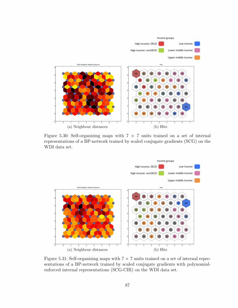
Income groups

High income: OECD

High income: nonOECD

Low income

Lower middle income

Upper middle income

−1 0 1 2 3 4 5 6 7−1

0

1

2

3

4

5

6

SOM Neighbor Weight Distances

(a) Neighbour distances

−1 0 1 2 3 4 5 6 7−1

0

1

2

3

4

5

6

43 28 43 33 36 28 18

38 27 32 5 41 34 263

48 12 11 28 10 31 16

11 22 37 14 14 41 29

43 16 35 7 14 17 45

12 28 18 14 4 11 40

250 22 27 25 42 22 45

Hits

(b) Hits

Figure 5.30: Self-organizing maps with 7 × 7 units trained on a set of internalrepresentations of a BP-network trained by scaled conjugate gradients (SCG) on theWDI data set.

Income groups

High income: OECD

High income: nonOECD

Low income

Lower middle income

Upper middle income

−1 0 1 2 3 4 5 6 7−1

0

1

2

3

4

5

6

SOM Neighbor Weight Distances

(a) Neighbour distances

−1 0 1 2 3 4 5 6 7−1

0

1

2

3

4

5

6

22 15 32 27 28 26 27

28 34 39 10 26 17 28

39 20 21 19 34 13 23

20 29 13 28 28 38 55

48 21 19 15 29 19 30

7 25 10 10 41 27 254

250 15 47 23 26 34 41

Hits

(b) Hits

Figure 5.31: Self-organizing maps with 7 × 7 units trained on a set of internal repre-sentations of a BP-network trained by scaled conjugate gradients with polynomial-enforced internal representations (SCG-CIR) on the WDI data set.

87

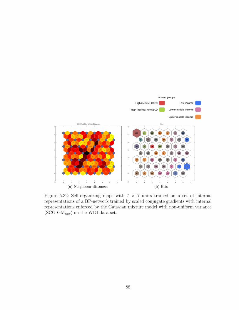
Income groups

High income: OECD

High income: nonOECD

Low income

Lower middle income

Upper middle income

−1 0 1 2 3 4 5 6 7−1

0

1

2

3

4

5

6

SOM Neighbor Weight Distances

(a) Neighbour distances

−1 0 1 2 3 4 5 6 7−1

0

1

2

3

4

5

6

52 30 20 29 28 53 35

18 21 11 25 18 27 122

33 23 23 33 27 27 36

26 25 15 9 35 38 38

64 26 28 23 25 37 40

21 61 23 29 18 44 64

207 26 29 14 17 34 23

Hits

(b) Hits

Figure 5.32: Self-organizing maps with 7 × 7 units trained on a set of internalrepresentations of a BP-network trained by scaled conjugate gradients with internalrepresentations enforced by the Gaussian mixture model with non-uniform variance(SCG-GMnuv) on the WDI data set.

88

Chapter 6

Conclusion

Artificial neural networks are a very successful model used to solve various types ofartificial intelligence problems in many domains. One of their main disadvantage isthat they are easily overfitted to a training data set which drastically limits theirgeneralization abilities. There exists a wide range of various methods to regularize thenetwork and thus limit its complexity and hinder the overfitting. This work exploresin detail one type of such regularizer, which forces internal representations in atrained network to take some predefined form. Enforced internal representations notonly effectively regularize neural networks but also provide a transparent structureof internal representations which are formed in trained networks.

This work explored the performance of BP-networks trained with different typesof enforced internal representations. The performance was evaluated on several dif-ferent tasks, both classification and regression. Two new regularizers were proposedto enforce internal representations in BP-network. The first regularizer is based onprobabilistic Gaussian mixture model and enforces a particular form of internal rep-resentations by modelling the probability density of internal representations by aproposed mixture model. It allows easy and flexible modelling of different types of in-ternal representations depending on the desired properties. Two of the possible formsof the Gaussian mixture regularizer, with uniform variance (homoscedastic model)and with non-uniform variance (heteroscedastic model), were extensively tested andcompared to the regularizer proposed in [?] and to the standard algorithms withoutenforced internal representations.

The second proposed regularizer uses the information theory to minimize theentropy of vectors of internal representations. The entropy of vectors is estimatedby nonparametric kernel density estimator (Parzen window), which is fully differen-tiable and therefore it also allows optimization by gradient descent based algorithms.The main advantage of the minimal entropy regularizer lies in the fact that it doesnot impose any particular form of internal representations and it leaves the internalrepresentations to take some form natural to a given training task. It only forcesnetworks to form as few different internal representations as possible. The perfor-mance of this regularizer was presented for the iris data set for the gradient descent

89

algorithm and the shape of internal representation it created were used as a basisof the Gaussian mixture model regularizer with non-uniform variance. Due to com-putational limitations, the minimal entropy regularizer was not studied on largerdata sets and it is left for further study. It would be also interesting to explorethe minimal-entropy configuration of internal representations formed by the scaledconjugate gradients algorithm.

Three of the presented regularizers, the condensed internal representations regu-larizer [?], the Gaussian mixture regularizer with uniform variances and the Gaussianmixture regularizer with non-uniform variance ,were tested on several different tasks.Their performance was compared both in terms of the performance on the trainingtasks and with respect to the formed internal representations. The data sets used forthe experiments comprised of an artificial problem of addition of binary numbers,three data sets from the UCI Machine Learning Repository and on real-world datafrom World Bank, the World Development Indicators.

In majority of the presented tasks, the networks with enforced internal representa-tions showed better performance than the standard optimization algorithms withoutregularization. The least difference in performance appeared for the regression taskon the World Bank data set. Generally, more significant difference was reached forthe presented classification tasks from the UCI repository.

The proposed Gaussian mixture regularizer with uniform variance showed mostlysimilar results as the condensed internal representations regularizer with polynomialcost function [?]. Slight variations appeared due to different shapes of their costfunctions, however they did not appear in a systematic way and depended on a givenparticular task. Both regularizer enforced the same form of internal representations.

The third proposed regularizer, Gaussian mixture model of internal represen-tations with non-uniform variance favoured the internal representations where themajority of activations were bipolar but the neurons were not strongly penalizedfor producing also activations with any different values. This regularizer showedvery good performance in most of the tasks, especially in combination with gradi-ent descent of gradient descent with momentum. It also helped the scaled conjugategradients algorithm to improve significantly in the artificial problem of binary ad-dition. It allowed networks to form more flexible mappings in the cases where theywere necessary. This regularizer was based on the activation patterns produced bythe minimal entropy regularizer. However, this regularizer does not produce as con-densed internal representations as the two other tested regularizers and thereforecannot serve as a basis for pruning algorithms.

New visualization methods were used to analyse the internal representation pat-terns formed by the discussed algorithms. This visualization was based on the self-organizing maps and allowed to explore the clusters of similar internal representationswith respect to target classes. This visualization method showed that well trainednetworks with good performance on a given data set are characterized by internalrepresentations clustered such that the clusters correspond to target classes/values.Similar classes were often clustered together of formed neighbouring clusters in the

90

self-organizing map.For the binary addition task, successful networks were able to form clusters of

internal representations such that they corresponded to the number of carry bitsneeded to compute the sum of binary numbers. The ability to deal with carry bitswas generally very difficult to learn.

For simple classification problems, such as the iris data set, internal represen-tations corresponded straightly to the target classes and mimicked the distributionof the input data in the feature space. For more complicated problems, the formedpatterns of internal representations were more diverse but again, the successful net-works were able to form distinctive internal representations for each of the targetclasses. For example, in the World Bank regression task, the networks distinguishedvery effectively the low income countries with low gross domestic product from thehigh income OECD countries. Also the distribution of internal representations in theself-organizing map corresponded to the relations in the data.

Generally, the clusters of formed internal representation allow to estimate thequality of prediction of the corresponding neural network. Especially for the classi-fication tasks, the clusters of internal representations formed by the networks withenforced internal representations were better defined and separated.

To conlude, the networks with enforced internal representations were more suc-cessful on the classification tasks than the unregularized networks. The reason of theirbetter performance lies in their ability to produce internal representations that areclustered into several groups for each of the target classes and mimic the distributionof the input data. This allows the networks to form robust functional mappings. Thenon-uniform Gaussian mixture regularizer, which was proposed in this work, showedbetter performance than other regularizers on most of the classification tasks. How-ever, the performance of the regularized networks on the studied regression task didnot differ significantly from the performance of the standard algorithms, which maybe also a result of effective preprocessing technique.

91

Appendix A

World development indicators

World development indicators CodeAdjusted net savings, excluding particulate emission damage (% ofGNI)

NY.ADJ.SVNX.GN.ZS

Adjusted net savings, including particulate emission damage (% ofGNI)

NY.ADJ.SVNG.GN.ZS

Adjusted savings: carbon dioxide damage (% of GNI) NY.ADJ.DCO2.GN.ZSAdjusted savings: consumption of fixed capital (% of GNI) NY.ADJ.DKAP.GN.ZSAdjusted savings: education expenditure (% of GNI) NY.ADJ.AEDU.GN.ZSAdjusted savings: energy depletion (% of GNI) NY.ADJ.DNGY.GN.ZSAdjusted savings: gross savings (% of GNI) NY.ADJ.ICTR.GN.ZSAdjusted savings: mineral depletion (% of GNI) NY.ADJ.DMIN.GN.ZSAdjusted savings: net forest depletion (% of GNI) NY.ADJ.DFOR.GN.ZSAdjusted savings: net national savings (% of GNI) NY.ADJ.NNAT.GN.ZSAdjusted savings: particulate emission damage (% of GNI) NY.ADJ.DPEM.GN.ZSAdolescent fertility rate (births per 1,000 women ages 15-19) SP.ADO.TFRTAge dependency ratio (% of working-age population) SP.POP.DPNDAge dependency ratio, old (% of working-age population) SP.POP.DPND.OLAge dependency ratio, young (% of working-age population) SP.POP.DPND.YGAgricultural employment (FAO) EN.AGR.EMPLAgricultural land (% of land area) AG.LND.AGRI.ZSAgricultural machinery, tractors per 100 sq. km of arable land AG.LND.TRAC.ZSAgricultural methane emissions (% of total) EN.ATM.METH.AG.ZSAgricultural nitrous oxide emissions (% of total) EN.ATM.NOXE.AG.ZSAgricultural raw materials exports (% of merchandise exports) TX.VAL.AGRI.ZS.UNAgricultural raw materials imports (% of merchandise imports) TM.VAL.AGRI.ZS.UNAgriculture value added per worker (constant 2000 US$) EA.PRD.AGRI.KDAgriculture, value added (% of GDP) NV.AGR.TOTL.ZSAgriculture, value added (annual % growth) NV.AGR.TOTL.KD.ZGAgriculture, value added (constant 2000 US$) NV.AGR.TOTL.KDAgriculture, value added (current US$) NV.AGR.TOTL.CDAir transport, freight (million ton-km) IS.AIR.GOOD.MT.K1Air transport, passengers carried IS.AIR.PSGRAir transport, registered carrier departures worldwide IS.AIR.DPRTAnimal species, threatened EN.ANM.THRD.NOAnnual freshwater withdrawals, agriculture (% of total freshwaterwithdrawal)

ER.H2O.FWAG.ZS

Annual freshwater withdrawals, domestic (% of total freshwater with-drawal)

ER.H2O.FWDM.ZS

Annual freshwater withdrawals, industry (% of total freshwater with-drawal)

ER.H2O.FWIN.ZS

Arable land (% of land area) AG.LND.ARBL.ZSArable land (hectares per person) AG.LND.ARBL.HA.PCArmed forces personnel (% of total labor force) MS.MIL.TOTL.TF.ZSArmed forces personnel, total MS.MIL.TOTL.P1Bank liquid reserves to bank assets ratio (%) FD.RES.LIQU.AS.ZS

92

Bird species, threatened EN.BIR.THRD.NOBird species, total known EN.BIR.TOTL.NOBirth rate, crude (per 1,000 people) SP.DYN.CBRT.INBusiness extent of disclosure index (0=less disclosure to 10=more dis-closure)

IC.BUS.DISC.XQ

Cereal yield (kg per hectare) AG.YLD.CREL.KGChanges in inventories (current US$) NE.GDI.STKB.CDChanges in net reserves (BoP, current US$) BN.RES.INCL.CDChildren out of school, primary SE.PRM.UNERChildren out of school, primary, female SE.PRM.UNER.FEChildren out of school, primary, male SE.PRM.UNER.MAClaims on governments and other public entities (current LCU) FM.AST.GOVT.CNClean energy production (% of total energy use) EG.USE.COMM.CL.ZSCO2 emissions (kg per 2000 US$ of GDP) EN.ATM.CO2E.KD.GDCO2 emissions (kg per 2005 PPP $ of GDP) EN.ATM.CO2E.PP.GD.KDCO2 emissions (kg per PPP $ of GDP) EN.ATM.CO2E.PP.GDCO2 emissions (metric tons per capita) EN.ATM.CO2E.PCCO2 emissions from solid fuel consumption (% of total) EN.ATM.CO2E.SF.ZSCO2 intensity (kg per kg of oil equivalent energy use) EN.ATM.CO2E.EG.ZSCombustible renewables and waste (% of total energy) EG.USE.CRNW.ZSCombustible renewables and waste (metric tons of oil equivalent) EG.USE.CRNW.KT.OECommercial service exports (current US$) TX.VAL.SERV.CD.WTCommercial service imports (current US$) TM.VAL.SERV.CD.WTComputer, communications and other services (% of commercial ser-vice exports)

TX.VAL.OTHR.ZS.WT

Computer, communications and other services (% of commercial ser-vice imports)

TM.VAL.OTHR.ZS.WT

Consumer price index (2005 = 100) FP.CPI.TOTLCost of business start-up procedures (% of GNI per capita) IC.REG.COST.PC.ZSCredit depth of information index (0=low to 6=high) IC.CRD.INFO.XQCrop production index (1999-2001 = 100) AG.PRD.CROP.XDCurrent account balance (% of GDP) BN.CAB.XOKA.GD.ZSCurrent account balance (BoP, current US$) BN.CAB.XOKA.CDCurrent transfers, receipts (BoP, current US$) BX.TRF.CURR.CDDeath rate, crude (per 1,000 people) SP.DYN.CDRT.INDeposit interest rate (%) FR.INR.DPSTDomestic credit provided by banking sector (% of GDP) FS.AST.DOMS.GD.ZSDomestic credit to private sector (% of GDP) FS.AST.PRVT.GD.ZSEase of doing business index (1=most business-friendly regulations) IC.BUS.EASE.XQElectric power consumption (kWh per capita) EG.USE.ELEC.KH.PCElectric power transmission and distribution losses (% of output) EG.ELC.LOSS.ZSElectricity production from coal sources (% of total) EG.ELC.COAL.ZSElectricity production from hydroelectric sources (% of total) EG.ELC.HYRO.ZSElectricity production from natural gas sources (% of total) EG.ELC.NGAS.ZSElectricity production from nuclear sources (% of total) EG.ELC.NUCL.ZSElectricity production from oil sources (% of total) EG.ELC.PETR.ZSEmigration rate of tertiary educated (% of total tertiary educatedpopulation)

SM.EMI.TERT.ZS

Employment to population ratio, ages 15-24, female (%) SL.EMP.1524.SP.FE.ZSEmployment to population ratio, ages 15-24, male (%) SL.EMP.1524.SP.MA.ZSEmployment to population ratio, ages 15-24, total (%) SL.EMP.1524.SP.ZSEnergy imports, net (% of energy use) EG.IMP.CONS.ZSEnergy use (kg of oil equivalent per capita) EG.USE.PCAP.KG.OEExports of goods and services (% of GDP) NE.EXP.GNFS.ZSExports of goods and services (annual % growth) NE.EXP.GNFS.KD.ZGExports of goods and services (BoP, current US$) BX.GSR.GNFS.CDExports of goods and services (constant 2000 US$) NE.EXP.GNFS.KDExports of goods and services (current US$) NE.EXP.GNFS.CDExports of goods, services and income (BoP, current US$) BX.GSR.TOTL.CDExternal balance on goods and services (% of GDP) NE.RSB.GNFS.ZSExternal balance on goods and services (current US$) NE.RSB.GNFS.CDExternal resources for health (% of total expenditure on health) SH.XPD.EXTR.ZSFemale adults with HIV (% of population ages 15+ with HIV) SH.DYN.AIDS.FE.ZSFertility rate, total (births per woman) SP.DYN.TFRT.IN

93

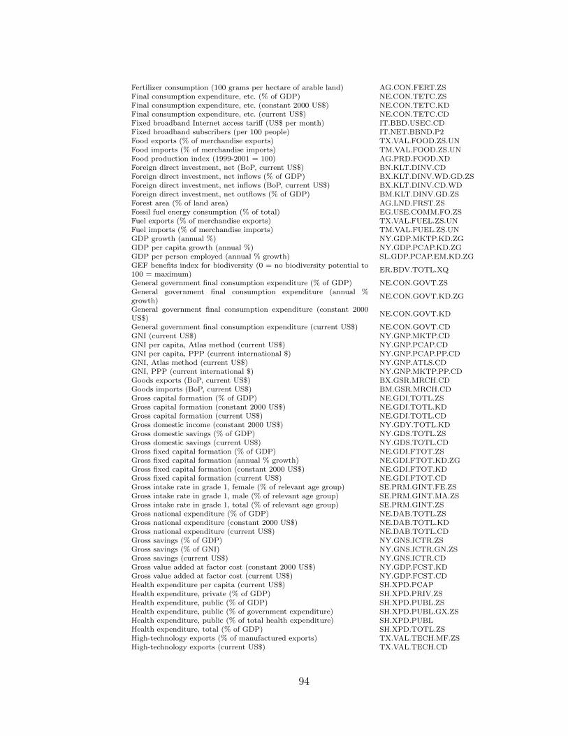
Fertilizer consumption (100 grams per hectare of arable land) AG.CON.FERT.ZSFinal consumption expenditure, etc. (% of GDP) NE.CON.TETC.ZSFinal consumption expenditure, etc. (constant 2000 US$) NE.CON.TETC.KDFinal consumption expenditure, etc. (current US$) NE.CON.TETC.CDFixed broadband Internet access tariff (US$ per month) IT.BBD.USEC.CDFixed broadband subscribers (per 100 people) IT.NET.BBND.P2Food exports (% of merchandise exports) TX.VAL.FOOD.ZS.UNFood imports (% of merchandise imports) TM.VAL.FOOD.ZS.UNFood production index (1999-2001 = 100) AG.PRD.FOOD.XDForeign direct investment, net (BoP, current US$) BN.KLT.DINV.CDForeign direct investment, net inflows (% of GDP) BX.KLT.DINV.WD.GD.ZSForeign direct investment, net inflows (BoP, current US$) BX.KLT.DINV.CD.WDForeign direct investment, net outflows (% of GDP) BM.KLT.DINV.GD.ZSForest area (% of land area) AG.LND.FRST.ZSFossil fuel energy consumption (% of total) EG.USE.COMM.FO.ZSFuel exports (% of merchandise exports) TX.VAL.FUEL.ZS.UNFuel imports (% of merchandise imports) TM.VAL.FUEL.ZS.UNGDP growth (annual %) NY.GDP.MKTP.KD.ZGGDP per capita growth (annual %) NY.GDP.PCAP.KD.ZGGDP per person employed (annual % growth) SL.GDP.PCAP.EM.KD.ZGGEF benefits index for biodiversity (0 = no biodiversity potential to100 = maximum)

ER.BDV.TOTL.XQ

General government final consumption expenditure (% of GDP) NE.CON.GOVT.ZSGeneral government final consumption expenditure (annual %growth)

NE.CON.GOVT.KD.ZG

General government final consumption expenditure (constant 2000US$)

NE.CON.GOVT.KD

General government final consumption expenditure (current US$) NE.CON.GOVT.CDGNI (current US$) NY.GNP.MKTP.CDGNI per capita, Atlas method (current US$) NY.GNP.PCAP.CDGNI per capita, PPP (current international $) NY.GNP.PCAP.PP.CDGNI, Atlas method (current US$) NY.GNP.ATLS.CDGNI, PPP (current international $) NY.GNP.MKTP.PP.CDGoods exports (BoP, current US$) BX.GSR.MRCH.CDGoods imports (BoP, current US$) BM.GSR.MRCH.CDGross capital formation (% of GDP) NE.GDI.TOTL.ZSGross capital formation (constant 2000 US$) NE.GDI.TOTL.KDGross capital formation (current US$) NE.GDI.TOTL.CDGross domestic income (constant 2000 US$) NY.GDY.TOTL.KDGross domestic savings (% of GDP) NY.GDS.TOTL.ZSGross domestic savings (current US$) NY.GDS.TOTL.CDGross fixed capital formation (% of GDP) NE.GDI.FTOT.ZSGross fixed capital formation (annual % growth) NE.GDI.FTOT.KD.ZGGross fixed capital formation (constant 2000 US$) NE.GDI.FTOT.KDGross fixed capital formation (current US$) NE.GDI.FTOT.CDGross intake rate in grade 1, female (% of relevant age group) SE.PRM.GINT.FE.ZSGross intake rate in grade 1, male (% of relevant age group) SE.PRM.GINT.MA.ZSGross intake rate in grade 1, total (% of relevant age group) SE.PRM.GINT.ZSGross national expenditure (% of GDP) NE.DAB.TOTL.ZSGross national expenditure (constant 2000 US$) NE.DAB.TOTL.KDGross national expenditure (current US$) NE.DAB.TOTL.CDGross savings (% of GDP) NY.GNS.ICTR.ZSGross savings (% of GNI) NY.GNS.ICTR.GN.ZSGross savings (current US$) NY.GNS.ICTR.CDGross value added at factor cost (constant 2000 US$) NY.GDP.FCST.KDGross value added at factor cost (current US$) NY.GDP.FCST.CDHealth expenditure per capita (current US$) SH.XPD.PCAPHealth expenditure, private (% of GDP) SH.XPD.PRIV.ZSHealth expenditure, public (% of GDP) SH.XPD.PUBL.ZSHealth expenditure, public (% of government expenditure) SH.XPD.PUBL.GX.ZSHealth expenditure, public (% of total health expenditure) SH.XPD.PUBLHealth expenditure, total (% of GDP) SH.XPD.TOTL.ZSHigh-technology exports (% of manufactured exports) TX.VAL.TECH.MF.ZSHigh-technology exports (current US$) TX.VAL.TECH.CD

94

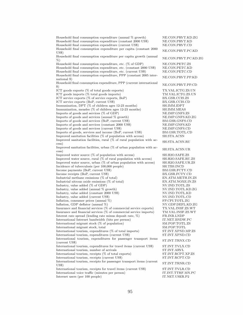
Household final consumption expenditure (annual % growth) NE.CON.PRVT.KD.ZGHousehold final consumption expenditure (constant 2000 US$) NE.CON.PRVT.KDHousehold final consumption expenditure (current US$) NE.CON.PRVT.CDHousehold final consumption expenditure per capita (constant 2000US$)

NE.CON.PRVT.PC.KD

Household final consumption expenditure per capita growth (annual%)

NE.CON.PRVT.PC.KD.ZG

Household final consumption expenditure, etc. (% of GDP) NE.CON.PETC.ZSHousehold final consumption expenditure, etc. (constant 2000 US$) NE.CON.PETC.KDHousehold final consumption expenditure, etc. (current US$) NE.CON.PETC.CDHousehold final consumption expenditure, PPP (constant 2005 inter-national $)

NE.CON.PRVT.PP.KD

Household final consumption expenditure, PPP (current international$)

NE.CON.PRVT.PP.CD

ICT goods exports (% of total goods exports) TX.VAL.ICTG.ZS.UNICT goods imports (% total goods imports) TM.VAL.ICTG.ZS.UNICT service exports (% of service exports, BoP) BX.GSR.CCIS.ZSICT service exports (BoP, current US$) BX.GSR.CCIS.CDImmunization, DPT (% of children ages 12-23 months) SH.IMM.IDPTImmunization, measles (% of children ages 12-23 months) SH.IMM.MEASImports of goods and services (% of GDP) NE.IMP.GNFS.ZSImports of goods and services (annual % growth) NE.IMP.GNFS.KD.ZGImports of goods and services (BoP, current US$) BM.GSR.GNFS.CDImports of goods and services (constant 2000 US$) NE.IMP.GNFS.KDImports of goods and services (current US$) NE.IMP.GNFS.CDImports of goods, services and income (BoP, current US$) BM.GSR.TOTL.CDImproved sanitation facilities (% of population with access) SH.STA.ACSNImproved sanitation facilities, rural (% of rural population with ac-cess)

SH.STA.ACSN.RU

Improved sanitation facilities, urban (% of urban population with ac-cess)

SH.STA.ACSN.UR

Improved water source (% of population with access) SH.H2O.SAFE.ZSImproved water source, rural (% of rural population with access) SH.H2O.SAFE.RU.ZSImproved water source, urban (% of urban population with access) SH.H2O.SAFE.UR.ZSIncidence of tuberculosis (per 100,000 people) SH.TBS.INCDIncome payments (BoP, current US$) BM.GSR.FCTY.CDIncome receipts (BoP, current US$) BX.GSR.FCTY.CDIndustrial methane emissions (% of total) EN.ATM.METH.IN.ZSIndustrial nitrous oxide emissions (% of total) EN.ATM.NOXE.IN.ZSIndustry, value added (% of GDP) NV.IND.TOTL.ZSIndustry, value added (annual % growth) NV.IND.TOTL.KD.ZGIndustry, value added (constant 2000 US$) NV.IND.TOTL.KDIndustry, value added (current US$) NV.IND.TOTL.CDInflation, consumer prices (annual %) FP.CPI.TOTL.ZGInflation, GDP deflator (annual %) NY.GDP.DEFL.KD.ZGInsurance and financial services (% of commercial service exports) TX.VAL.INSF.ZS.WTInsurance and financial services (% of commercial service imports) TM.VAL.INSF.ZS.WTInterest rate spread (lending rate minus deposit rate, %) FR.INR.LNDPInternational Internet bandwidth (bits per person) IT.NET.BNDW.PCInternational migrant stock (% of population) SM.POP.TOTL.ZSInternational migrant stock, total SM.POP.TOTLInternational tourism, expenditures (% of total imports) ST.INT.XPND.MP.ZSInternational tourism, expenditures (current US$) ST.INT.XPND.CDInternational tourism, expenditures for passenger transport items(current US$)

ST.INT.TRNX.CD

International tourism, expenditures for travel items (current US$) ST.INT.TVLX.CDInternational tourism, number of arrivals ST.INT.ARVLInternational tourism, receipts (% of total exports) ST.INT.RCPT.XP.ZSInternational tourism, receipts (current US$) ST.INT.RCPT.CDInternational tourism, receipts for passenger transport items (currentUS$)

ST.INT.TRNR.CD

International tourism, receipts for travel items (current US$) ST.INT.TVLR.CDInternational voice traffic (minutes per person) IT.INT.TTRF.MN.PCInternet users (per 100 people) IT.NET.USER.P2

95

Irrigated land (% of cropland) AG.LND.IRIG.ZSLabor force, female (% of total labor force) SL.TLF.TOTL.FE.ZSLabor participation rate, female (% of female population ages 15+) SL.TLF.CACT.FE.ZSLabor participation rate, male (a% of male population ages 15+) SL.TLF.CACT.MA.ZSLabor participation rate, total (% of total population ages 15+) SL.TLF.CACT.ZSLand under cereal production (hectares) AG.LND.CREL.HALending interest rate (%) FR.INR.LENDLife expectancy at birth, female (years) SP.DYN.LE00.FE.INLife expectancy at birth, male (years) SP.DYN.LE00.MA.INLife expectancy at birth, total (years) SP.DYN.LE00.INLifetime risk of maternal death (1 in: rate varies by country) SH.MMR.RISKLivestock production index (1999-2001 = 100) AG.PRD.LVSK.XDManufactures exports (% of merchandise exports) TX.VAL.MANF.ZS.UNManufactures imports (% of merchandise imports) TM.VAL.MANF.ZS.UNManufacturing, value added (% of GDP) NV.IND.MANF.ZSManufacturing, value added (annual % growth) NV.IND.MANF.KD.ZGManufacturing, value added (constant 2000 US$) NV.IND.MANF.KDManufacturing, value added (current US$) NV.IND.MANF.CDMaternal mortality ratio (modeled estimate, per 100,000 live births) SH.STA.MMRTMerchandise exports (current US$) TX.VAL.MRCH.CD.WTMerchandise imports (current US$) TM.VAL.MRCH.CD.WTMerchandise trade (% of GDP) TG.VAL.TOTL.GD.ZSMilitary expenditure (% of GDP) MS.MIL.XPND.GD.ZSMobile and fixed-line telephone subscribers (per 100 people) IT.TEL.TOTL.P2Mobile and fixed-line telephone subscribers per employee IT.TEL.TOTL.EMMobile cellular prepaid tariff (US$ per month) IT.MBL.USEC.CDMobile cellular subscriptions (per 100 people) IT.CEL.SETS.P2Mortality rate, adult, female (per 1,000 female adults) SP.DYN.AMRT.FEMortality rate, adult, male (per 1,000 male adults) SP.DYN.AMRT.MAMortality rate, infant (per 1,000 live births) SP.DYN.IMRT.INMortality rate, under-5 (per 1,000) SH.DYN.MORTNationally protected areas (% of total land area) ER.LND.PTLD.ZSNet capital account (BoP, current US$) BN.TRF.KOGT.CDNet current transfers (BoP, current US$) BN.TRF.CURR.CDNet current transfers from abroad (current US$) NY.TRF.NCTR.CDNet errors and omissions, adjusted (BoP, current US$) BN.KAC.EOMS.CDNet income (BoP, current US$) BN.GSR.FCTY.CDNet income from abroad (current US$) NY.GSR.NFCY.CDNet migration SM.POP.NETMNet taxes on products (current US$) NY.TAX.NIND.CDNet trade in goods (BoP, current US$) BN.GSR.MRCH.CDNet trade in goods and services (BoP, current US$) BN.GSR.GNFS.CDNitrous oxide emissions (thousand metric tons of CO2 equivalent) EN.ATM.NOXE.KT.CEOres and metals exports (% of merchandise exports) TX.VAL.MMTL.ZS.UNOres and metals imports (% of merchandise imports) TM.VAL.MMTL.ZS.UNOut-of-pocket health expenditure (% of private expenditure on health) SH.XPD.OOPC.ZSPermanent cropland (% of land area) AG.LND.CROP.ZSPersonal computers (per 100 people) IT.CMP.PCMP.P2Plant species (higher), threatened EN.HPT.THRD.NOPlant species (higher), total known EN.HPT.TOTL.NOPM10, country level (micrograms per cubic meter) EN.ATM.PM10.MC.M3Population ages 0-14 (% of total) SP.POP.0014.TO.ZSPopulation ages 15-64 (% of total) SP.POP.1564.TO.ZSPopulation ages 65 and above (% of total) SP.POP.65UP.TO.ZSPopulation covered by mobile cellular network (%) IT.CEL.COVR.ZSPopulation density (people per sq. km) EN.POP.DNSTPopulation growth (annual %) SP.POP.GROWPopulation, female (% of total) SP.POP.TOTL.FE.ZSPortfolio investment, equity (DRS, current US$) BX.PEF.TOTL.CD.DTPortfolio investment, excluding LCFAR (BoP, current US$) BN.KLT.PTXL.CDPrevalence of HIV, female (% ages 15-24) SH.HIV.1524.FE.ZSPrevalence of HIV, male (% ages 15-24) SH.HIV.1524.MA.ZSPrevalence of HIV, total (% of population ages 15-49) SH.DYN.AIDS.ZSPrevalence of undernourishment (% of population) SN.ITK.DEFC.ZS

96

Primary completion rate, female (% of relevant age group) SE.PRM.CMPT.FE.ZSPrimary completion rate, male (% of relevant age group) SE.PRM.CMPT.MA.ZSPrimary completion rate, total (% of relevant age group) SE.PRM.CMPT.ZSPrimary education, duration (years) SE.PRM.DURSPrimary education, pupils (% female) SE.PRM.ENRL.FE.ZSPrimary education, teachers (% female) SE.PRM.TCHR.FE.ZSPrimary school starting age (years) SE.PRM.AGESPrivate credit bureau coverage (% of adults) IC.CRD.PRVT.ZSProcedures to build a warehouse (number) IC.WRH.PROCProcedures to enforce a contract (number) IC.LGL.PROCProcedures to register property (number) IC.PRP.PROCProportion of seats held by women in national parliaments (%) SG.GEN.PARL.ZSPublic credit registry coverage (% of adults) IC.CRD.PUBL.ZSPublic spending on education, total (% of GDP) SE.XPD.TOTL.GD.ZSPump price for diesel fuel (US$ per liter) EP.PMP.DESL.CDPump price for gasoline (US$ per liter) EP.PMP.SGAS.CDPupil-teacher ratio, primary SE.PRM.ENRL.TC.ZSPupil-teacher ratio, secondary SE.SEC.ENRL.TC.ZSRatio of female to male enrollments in tertiary education SE.ENR.TERT.FM.ZSRatio of female to male primary enrollment SE.ENR.PRIM.FM.ZSRatio of female to male secondary enrollment SE.ENR.SECO.FM.ZSRatio of girls to boys in primary and secondary education (%) SE.ENR.PRSC.FM.ZSReal interest rate (%) FR.INR.RINRRenewable internal freshwater resources per capita (cubic meters) ER.H2O.INTR.PCRepetition rate, primary (% of total enrollment) SE.PRM.REPT.ZSRepetition rate, primary, female (% of total enrollment) SE.PRM.REPT.FE.ZSRepetition rate, primary, male (% of total enrollment) SE.PRM.REPT.MA.ZSResidential fixed line telephone tariff (US$ per month) IT.RES.USEC.CDRigidity of employment index (0=less rigid to 100=more rigid) IC.LGL.EMPL.XQRoad sector fuel consumption (% of total consumption) IS.ROD.ENGY.ZSRoad sector fuel consumption per capita (liters) IS.ROD.ENGY.PCRoyalty and license fees, payments (BoP, current US$) BM.GSR.ROYL.CDRural population (% of total population) SP.RUR.TOTL.ZSRural population density (rural population per sq. km of arable land) EN.RUR.DNSTRural population growth (annual %) SP.RUR.TOTL.ZGSchool enrollment, preprimary (% gross) SE.PRE.ENRRSchool enrollment, preprimary, female (% gross) SE.PRE.ENRR.FESchool enrollment, preprimary, male (% gross) SE.PRE.ENRR.MASchool enrollment, primary (% gross) SE.PRM.ENRRSchool enrollment, primary (% net) SE.PRM.NENRSchool enrollment, primary, female (% gross) SE.PRM.ENRR.FESchool enrollment, primary, female (% net) SE.PRM.NENR.FESchool enrollment, primary, male (% gross) SE.PRM.ENRR.MASchool enrollment, primary, male (% net) SE.PRM.NENR.MASchool enrollment, primary, private (% of total primary) SE.PRM.PRIV.ZSSchool enrollment, secondary (% gross) SE.SEC.ENRRSchool enrollment, secondary, female (% gross) SE.SEC.ENRR.FESchool enrollment, secondary, male (% gross) SE.SEC.ENRR.MASchool enrollment, secondary, private (% of total secondary) SE.SEC.PRIV.ZSSchool enrollment, tertiary (% gross) SE.TER.ENRRSchool enrollment, tertiary, female (% gross) SE.TER.ENRR.FESchool enrollment, tertiary, male (% gross) SE.TER.ENRR.MASecondary education, duration (years) SE.SEC.DURSSecondary education, general pupils (% female) SE.SEC.ENRL.GC.FE.ZSSecondary education, pupils (% female) SE.SEC.ENRL.FE.ZSSecondary education, teachers (% female) SE.SEC.TCHR.FE.ZSSecondary education, vocational pupils (% female) SE.SEC.ENRL.VO.FE.ZSSecondary school starting age (years) SE.SEC.AGESSecure Internet servers (per 1 million people) IT.NET.SECR.P6Service exports (BoP, current US$) BX.GSR.NFSV.CDService imports (BoP, current US$) BM.GSR.NFSV.CDServices, etc., value added (% of GDP) NV.SRV.TETC.ZSServices, etc., value added (annual % growth) NV.SRV.TETC.KD.ZGServices, etc., value added (constant 2000 US$) NV.SRV.TETC.KD

97

Services, etc., value added (current US$) NV.SRV.TETC.CDSmoking prevalence, females (% of adults) SH.PRV.SMOK.FESmoking prevalence, males (% of adults) SH.PRV.SMOK.MAStart-up procedures to register a business (number) IC.REG.PROCStrength of legal rights index (0=weak to 10=strong) IC.LGL.CRED.XQSurface area (sq. km) AG.SRF.TOTL.K2Survival to age 65, female (% of cohort) SP.DYN.TO65.FE.ZSSurvival to age 65, male (% of cohort) SP.DYN.TO65.MA.ZSTelecommunications investment (% of revenue) IT.TEL.INVS.RV.ZSTelecommunications revenue (% GDP) IT.TEL.REVN.GD.ZSTelephone lines (per 100 people) IT.MLT.MAIN.P2Time required to build a warehouse (days) IC.WRH.DURSTime required to enforce a contract (days) IC.LGL.DURSTime required to register property (days) IC.PRP.DURSTime required to start a business (days) IC.REG.DURSTime to prepare and pay taxes (hours) IC.TAX.DURSTime to resolve insolvency (years) IC.ISV.DURSTotal enrollment, primary (% net) SE.PRM.TENRTotal enrollment, primary, female (% net) SE.PRM.TENR.FETotal enrollment, primary, male (% net) SE.PRM.TENR.MATotal reserves (includes gold, current US$) FI.RES.TOTL.CDTotal reserves in months of imports FI.RES.TOTL.MOTotal reserves minus gold (current US$) FI.RES.XGLD.CDTotal tax rate (% of profit) IC.TAX.TOTL.CP.ZSTrade (% of GDP) NE.TRD.GNFS.ZSTrade in services (% of GDP) BG.GSR.NFSV.GD.ZSTransport sector diesel fuel consumption per capita (liters) IS.ROD.DESL.PCTransport sector gasoline fuel consumption per capita (liters) IS.ROD.SGAS.PCTransport services (% of commercial service exports) TX.VAL.TRAN.ZS.WTTransport services (% of commercial service imports) TM.VAL.TRAN.ZS.WTTravel services (% of commercial service exports) TX.VAL.TRVL.ZS.WTTravel services (% of commercial service imports) TM.VAL.TRVL.ZS.WTTuberculosis cases detected under DOTS (%) SH.TBS.DOTSTuberculosis treatment success rate (% of registered cases) SH.TBS.CURE.ZSUrban population (% of total) SP.URB.TOTL.IN.ZSUrban population growth (annual %) SP.URB.GROWWorkers’ remittances and compensation of employees, paid (currentUS$)

BM.TRF.PWKR.CD.DT

Workers’ remittances and compensation of employees, received (% ofGDP)

BX.TRF.PWKR.DT.GD.ZS

Workers’ remittances and compensation of employees, received (cur-rent US$)

BX.TRF.PWKR.CD.DT

Workers’ remittances, receipts (BoP, current US$) BX.TRF.PWKR.CD

98

Appendix B

Countries

Country Code Income group

Albania ALB Upper middle incomeAlgeria DZA Upper middle incomeAngola AGO Lower middle incomeArgentina ARG Upper middle incomeArmenia ARM Lower middle incomeAustralia AUS High income: OECDAustria AUT High income: OECDAzerbaijan AZE Upper middle incomeBahamas, The BHS High income: nonOECDBahrain BHR High income: nonOECDBangladesh BGD Low incomeBarbados BRB High income: nonOECDBelarus BLR Upper middle incomeBelgium BEL High income: OECDBelize BLZ Lower middle incomeBenin BEN Low incomeBhutan BTN Lower middle incomeBolivia BOL Lower middle incomeBosnia and Herzegovina BIH Upper middle incomeBotswana BWA Upper middle incomeBrazil BRA Upper middle incomeBrunei Darussalam BRN High income: nonOECDBulgaria BGR Upper middle incomeBurkina Faso BFA Low incomeBurundi BDI Low incomeCambodia KHM Low incomeCameroon CMR Lower middle incomeCanada CAN High income: OECDCape Verde CPV Lower middle incomeCentral African Repub-lic

CAF Low income

99

Colombia COL Upper middle incomeComoros COM Low incomeCongo, Dem. Rep. ZAR Low incomeCongo, Rep. COG Lower middle incomeCosta Rica CRI Upper middle incomeCote d’Ivoire CIV Lower middle incomeCroatia HRV High income: nonOECDCyprus CYP High income: nonOECDCzech Republic CZE High income: OECDDenmark DNK High income: OECDDjibouti DJI Lower middle incomeDominica DMA Upper middle incomeDominican Republic DOM Upper middle incomeEcuador ECU Lower middle incomeEgypt, Arab Rep. EGY Lower middle incomeEl Salvador SLV Lower middle incomeEritrea ERI Low incomeEstonia EST High income: nonOECDEthiopia ETH Low incomeFiji FJI Upper middle incomeFinland FIN High income: OECDFrance FRA High income: OECDGabon GAB Upper middle incomeGambia, The GMB Low incomeGeorgia GEO Lower middle incomeGermany DEU High income: OECDGhana GHA Low incomeGreece GRC High income: OECDGrenada GRD Upper middle incomeGuatemala GTM Lower middle incomeGuinea GIN Low incomeGuinea-Bissau GNB Low incomeGuyana GUY Lower middle incomeHaiti HTI Low incomeHonduras HND Lower middle incomeHong Kong, China HKG High income: nonOECDHungary HUN High income: OECDChad TCD Low incomeChile CHL Upper middle incomeChina CHN Lower middle incomeIceland ISL High income: OECDIndia IND Lower middle incomeIndonesia IDN Lower middle incomeIran, Islamic Rep. IRN Upper middle incomeIreland IRL High income: OECD

100

Israel ISR High income: nonOECDItaly ITA High income: OECDJamaica JAM Upper middle incomeJapan JPN High income: OECDJordan JOR Lower middle incomeKazakhstan KAZ Upper middle incomeKenya KEN Low incomeKorea, Rep. KOR High income: OECDKuwait KWT High income: nonOECDKyrgyz Republic KGZ Low incomeLao PDR LAO Low incomeLatvia LVA High income: nonOECDLebanon LBN Upper middle incomeLesotho LSO Lower middle incomeLithuania LTU Upper middle incomeLuxembourg LUX High income: OECDMacao, China MAC High income: nonOECDMacedonia, FYR MKD Upper middle incomeMadagascar MDG Low incomeMalawi MWI Low incomeMalaysia MYS Upper middle incomeMaldives MDV Lower middle incomeMali MLI Low incomeMalta MLT High income: nonOECDMauritania MRT Low incomeMauritius MUS Upper middle incomeMexico MEX Upper middle incomeMoldova MDA Lower middle incomeMongolia MNG Lower middle incomeMorocco MAR Lower middle incomeMozambique MOZ Low incomeMyanmar MMR Low incomeNamibia NAM Upper middle incomeNepal NPL Low incomeNetherlands NLD High income: OECDNew Zealand NZL High income: OECDNicaragua NIC Lower middle incomeNiger NER Low incomeNigeria NGA Lower middle incomeNorway NOR High income: OECDOman OMN High income: nonOECDPakistan PAK Lower middle incomePanama PAN Upper middle incomePapua New Guinea PNG Lower middle incomeParaguay PRY Lower middle income

101

Peru PER Upper middle incomePhilippines PHL Lower middle incomePoland POL High income: OECDPortugal PRT High income: OECDRomania ROM Upper middle incomeRussian Federation RUS Upper middle incomeRwanda RWA Low incomeSamoa WSM Lower middle incomeSao Tome and Principe STP Lower middle incomeSaudi Arabia SAU High income: nonOECDSenegal SEN Lower middle incomeSerbia SRB Upper middle incomeSeychelles SYC Upper middle incomeSierra Leone SLE Low incomeSingapore SGP High income: nonOECDSlovak Republic SVK High income: OECDSlovenia SVN High income: nonOECDSolomon Islands SLB Low incomeSouth Africa ZAF Upper middle incomeSpain ESP High income: OECDSri Lanka LKA Lower middle incomeSt. Kitts and Nevis KNA Upper middle incomeSt. Lucia LCA Upper middle incomeSt. Vincent and theGrenadines

VCT Upper middle income

Sudan SDN Lower middle incomeSuriname SUR Upper middle incomeSwaziland SWZ Lower middle incomeSweden SWE High income: OECDSwitzerland CHE High income: OECDSyrian Arab Republic SYR Lower middle incomeTajikistan TJK Low incomeTanzania TZA Low incomeThailand THA Lower middle incomeTogo TGO Low incomeTonga TON Lower middle incomeTrinidad and Tobago TTO High income: nonOECDTunisia TUN Lower middle incomeTurkey TUR Upper middle incomeTurkmenistan TKM Lower middle incomeUganda UGA Low incomeUkraine UKR Lower middle incomeUnited Arab Emirates ARE High income: nonOECDUnited Kingdom GBR High income: OECDUnited States USA High income: OECD

102

Uruguay URY Upper middle incomeUzbekistan UZB Lower middle incomeVanuatu VUT Lower middle incomeVenezuela, RB VEN Upper middle incomeVietnam VNM Lower middle incomeWest Bank and Gaza WBG Lower middle incomeYemen, Rep. YEM Lower middle incomeZambia ZMB Low incomeZimbabwe ZWE Low income

103

Bibliography

[1] Y. S. Abu-Mostafa. Learning from hints. Journal of Complexity, 10(1):165–178, 1994.

[2] Y. S. Abu-Mostafa. Hints. Neural Computation, 7(4):639–671, 1995.

[3] H. Altun, A. Bilgil, and B. C. Fidan. Treatment of multi-dimensional data to enhance neural network estimatorsin regression problems. Expert Syst. Appl., 32(2):599–605, 2007.

[4] H. Altun, A. Bilgil, and B. C. Fidan. Treatment of skewed multi-dimensional training data to facilitate thetask of engineering neural models. Expert Syst. Appl., 33(4):978–983, 2007.

[5] B. Baesens, S. Viaene, J. Vanthienen, and G. Dedene. Wrapped feature selection by means of guided neuralnetwork optimization. In ICPR, pages 2113–2116, 2000.

[6] C. M. Bishop. Neural networks for pattern recognition. Oxford University Press, 1996.

[7] A. L. Blum and P. Langley. Selection of relevant features and examples in machine learning. Artificial Intelli-gence, 97:245–271, 1997.

[8] Y. L. Cun, J. S. Denker, and S. A. Solla. Optimal brain damage. In Advances in Neural Information ProcessingSystems, pages 598–605, 1990.

[9] A. Engelbrecht. A new pruning heuristic based on variance analysis of sensitivity information. IEEE Transac-tions on Neural Networks, 12:1386–1399, 2001.

[10] A. Engelbrecht and I. Cloete. A sensitivity analysis algorithm for pruning feedforward neural networks. InIEEE International Conference in Neural Networks, pages 1274–1277, 1996.

[11] A. P. Engelbrecht, L. Fletcher, and I. Cloete. Variance analysis of sensitivity information for pruning multilayerfeedforward neural networks. In Proceedings of IEEE IJCNN, volume 3, pages 1829–1833, 1999.

[12] O. Gallmo and J. Carlstrom. Some experiments using extra output learning to hint multi layer perceptrons. InCurrent Trends in Connectionism, pages 179–190, 1995.

[13] I. Guyon and A. Elisseeff. An introduction to variable and feature selection. Journal of Machine LearningResearch, 3:1157–1182, 2003.

[14] I. Guyon, S. Gunn, A. Ben-Hur, and G. Dror. Result analysis of the nips 2003 feature selection challenge. InAdvances in Neural Information Processing Systems 17, pages 545–552. MIT Press, Cambridge, MA, 2005.

[15] B. Hassibi, D. Stork, and G. Wolff. Optimal brain surgeon and general network pruning. In IEEE InternationalConference on Neural Networks, pages 293 – 299, 1993.

[16] T. Hastie, R. Tibshirani, G. Sherlock, M. Eisen, P. Brown, and D. Botstein. Imputing missing data for geneexpression arrays. Technical report, Division of Biostatistics, Stanford University, 1999.

[17] J. Honaker and G. King. What to do about missing values in time series cross-section data, 2006.

[18] R. Kohavi and G. H. John. Wrappers for feature subset selection. Artificial Intelligence, 97:273–324, 1997.

[19] U. A. Kumar. Comparison of neural networks and regression analysis: A new insight. Expert Syst. Appl.,29(2):424–430, 2005.

104

[20] M. Leshno, V. Y. Lin, A. Pinkus, and S. Schocken. Multilayer feedforward networks with a nonpolynomialactivation function can approximate any function. Neural Networks, 6:861–867, 1993.

[21] T. Mitchell. Machine Learning. McGraw-Hill Education (ISE Editions), 1997.

[22] M. F. Moller. A scaled conjugate gradient algorithm for fast supervised learning. Neural Networks, 6:525–533,1993.

[23] J. J. Montano and A. Palmer. Numeric sensitivity analysis applied to feedforward neural networks. NeuralComputing and Applications, 12:119–125, 2003.

[24] I. Mrazova and D. Wang. Improved generalization of neural classifiers with enforced internal representation.Neurocomputing, 70:2940–2952, 2007.

[25] I. Mrazova and Z. Reitermanova. Enforced knowledge extraction with bp-networks. In Intelligent EngineeringSystems through Artificial Neural Network, volume 17, pages 285–290, 2007.

[26] L. Prechelt. Automatic early stopping using cross validation: Quantifying the criteria. Neural Networks, 11:761–767, 1997.

[27] J. Sietsma and R. J. F. Dow. Creating artificial neural networks that generalize. Neural Networks, 4:67–79,1991.

[28] S. C. Suddarth and Y. L. Kergosien. Rule-injection hints as a means of improving network performance andlearning time. In Proceedings of the EURASIP Workshop 1990 on Neural Networks, pages 120–129, 1990.

[29] T. Tchaban, M. Taylor, and J. Griffin. Establishing impacts of the inputs in a feedforward neural network.Neural Computing and Applications, 7:309–317, 1998.

[30] W. Wang, P. Jones, and D. Partridge. Assessing the impact of input features in a feedforward neural network.Neural Computing and Applications, 9:101–112, 2000.

[31] J. M. Zurada, A. Malinowski, and I. Cloete. Sensitivity analysis for minimization of input data dimensionforfeedforward neural network. IEEE International Symposium on Circuits and Systems, 6:447–450, 1994.

105