Discussion Papers In Economics And Business

Graduate School of Economics and Osaka School of International Public Policy (OSIPP)

Osaka University, Toyonaka, Osaka 560-0043, JAPAN

Aging, Pensions, and Growth

Tetsuo Ono

Discussion Paper 14-17-Rev.2

June 2016

Graduate School of Economics and Osaka School of International Public Policy (OSIPP)

Osaka University, Toyonaka, Osaka 560-0043, JAPAN

Aging, Pensions, and Growth

Tetsuo Ono

Discussion Paper 14-17-Rev.2

Aging, Pensions, and Growth∗

Tetsuo Ono†

Osaka University

Abstract

This study presents an endogenous growth, overlapping-generations model fea-turing probabilistic voting over public pensions. The analysis shows that (i) thepension–GDP ratio increases as life expectancy increases in the presence of an an-nuity market, while it may show a hump-shaped pattern in its absence; (ii) thegrowth rate is higher in the presence of the annuity market than its absence, butthe presence implies an intergenerational trade-off in terms of utility.

Keywords: Economic Growth; Population Aging; Probabilistic Voting; PublicPensions; Annuity Market

JEL Classification: D70, E24, H55

∗This paper is a substantially revised version of an earlier paper entitled “Economic Growth and thePolitics of Intergenerational Redistribution.” This work was supported in part by a Grant-in-Aid forScientific Research (C) from the Ministry of Education, Science and Culture of Japan No. 15K03509.The author would like to thank Yuki Uchida for his research assistance.

†Graduate School of Economics, Osaka University, 1-7, Machikaneyama, Toyonaka, Osaka 560-0043,Japan. Tel.: +81-6-6850-6111; Fax: +81-6-6850-5256. E-mail: tono@econ.osaka-u.ac.jp

1 Introduction

Many Organisation for Economic Co-operation and Development (OECD) countries have

experienced declining population growth rates and increasing life expectancy over the past

decades (OECD, 2011). This demographic change raises the share of the elderly in the

population, which is expected to strengthen their political power in voting. Therefore,

government spending for the elderly, such as on public pensions and long-term care, is

likely to increase. One of the expected side effects of this trend is an increase in the tax

burden on the young, which may result in a declining growth rate over time.

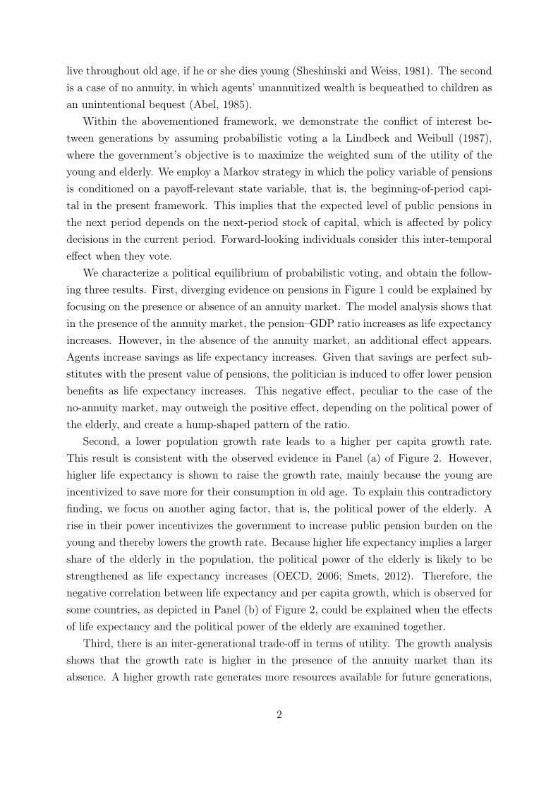
The prediction about the effect of population decline on pensions is in line with ob-

servations in OECD countries. Panel (a) of Figure 1 suggests that the public pension

spending–GDP ratio is positively correlated to the declining population growth rate. On

the other hand, the aforementioned prediction on the effect of increasing life expectancy is

not likely to fit the observation. In Panel (b) of Figure 1, the pension–GDP ratio shows a

weak positive correlation with increasing life expectancy. However, France and Italy show

more than five times higher ratios than Iceland, Israel, and Mexico, although they all

share similar life expectancy. Therefore, the empirical evidence seems to be mixed. The

first aim of this study is to present a political economy theory that explains the diverging

evidence observed in Figure 1.

[Figure 1 here.]

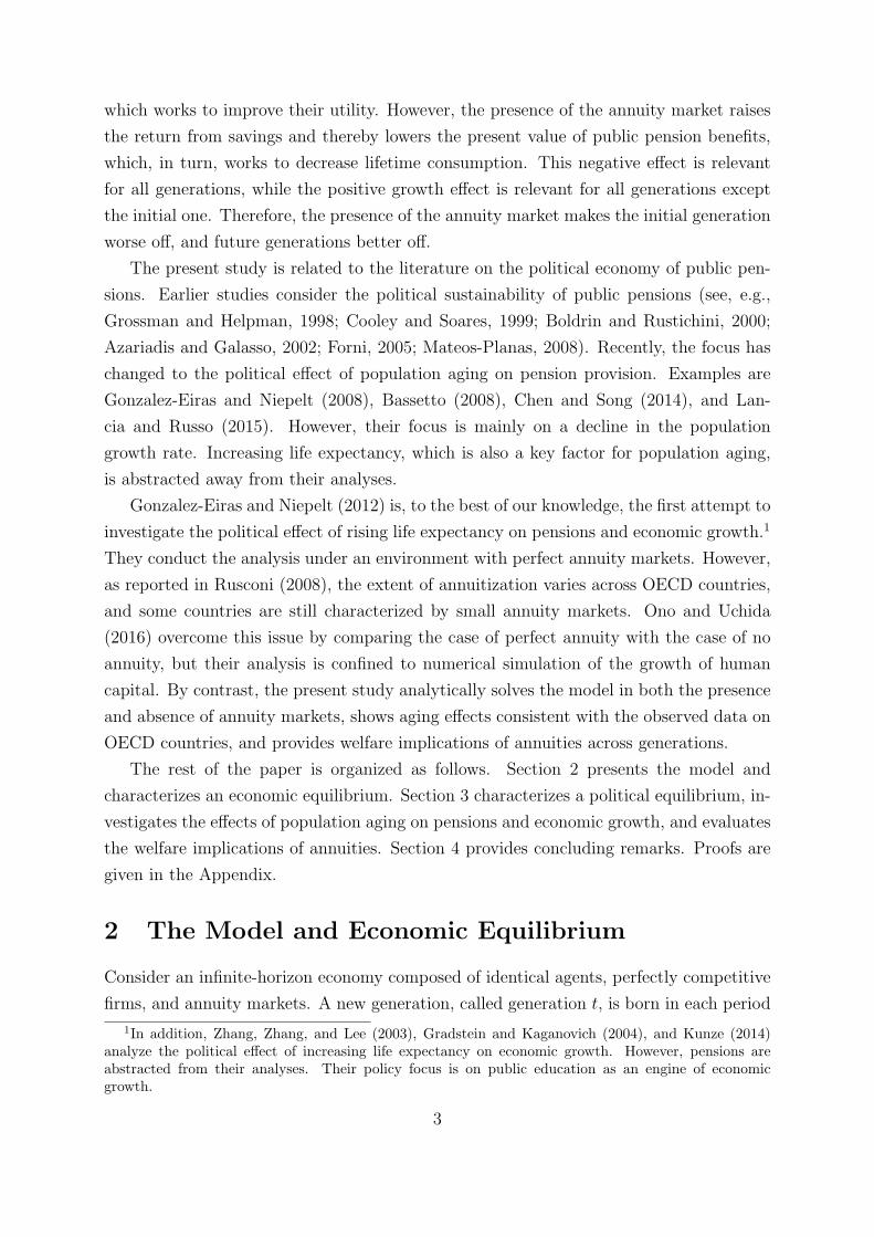
The second aim is to provide a theory that fits the evidence on aging and economic

growth. The aforementioned argument suggests that lower population growth has a neg-

ative effect on economic growth because of increasing pension burden. However, the

evidence in Panel (a) of Figure 2 shows that lower population growth is associated with

higher per capita GDP growth. In addition, increasing life expectancy is associated with

lower per capita GDP growth, as depicted in Panel (b) of Figure 2. The two aging factors

have opposite implications for economic growth. The present study demonstrates a model

that explains these contradictory results.

[Figure 2 here.]

For the aims of this study, we develop an overlapping-generations model with individ-

uals who live for a maximum of two periods, youth and old age, and competitive firms

endowed with AK technology, as in Romer (1986). Government spending financed by a

tax on the young includes public pensions that benefit the elderly. Within this frame-

work, we consider and compare the following two cases. The first is a perfect annuity

case in which an agent’s wealth is annuitized and transferred to the other agents, who

1

live throughout old age, if he or she dies young (Sheshinski and Weiss, 1981). The second

is a case of no annuity, in which agents’ unannuitized wealth is bequeathed to children as

an unintentional bequest (Abel, 1985).

Within the abovementioned framework, we demonstrate the conflict of interest be-

tween generations by assuming probabilistic voting a la Lindbeck and Weibull (1987),

where the government’s objective is to maximize the weighted sum of the utility of the

young and elderly. We employ a Markov strategy in which the policy variable of pensions

is conditioned on a payoff-relevant state variable, that is, the beginning-of-period capi-

tal in the present framework. This implies that the expected level of public pensions in

the next period depends on the next-period stock of capital, which is affected by policy

decisions in the current period. Forward-looking individuals consider this inter-temporal

effect when they vote.

We characterize a political equilibrium of probabilistic voting, and obtain the follow-

ing three results. First, diverging evidence on pensions in Figure 1 could be explained by

focusing on the presence or absence of an annuity market. The model analysis shows that

in the presence of the annuity market, the pension–GDP ratio increases as life expectancy

increases. However, in the absence of the annuity market, an additional effect appears.

Agents increase savings as life expectancy increases. Given that savings are perfect sub-

stitutes with the present value of pensions, the politician is induced to offer lower pension

benefits as life expectancy increases. This negative effect, peculiar to the case of the

no-annuity market, may outweigh the positive effect, depending on the political power of

the elderly, and create a hump-shaped pattern of the ratio.

Second, a lower population growth rate leads to a higher per capita growth rate.

This result is consistent with the observed evidence in Panel (a) of Figure 2. However,

higher life expectancy is shown to raise the growth rate, mainly because the young are

incentivized to save more for their consumption in old age. To explain this contradictory

finding, we focus on another aging factor, that is, the political power of the elderly. A

rise in their power incentivizes the government to increase public pension burden on the

young and thereby lowers the growth rate. Because higher life expectancy implies a larger

share of the elderly in the population, the political power of the elderly is likely to be

strengthened as life expectancy increases (OECD, 2006; Smets, 2012). Therefore, the

negative correlation between life expectancy and per capita growth, which is observed for

some countries, as depicted in Panel (b) of Figure 2, could be explained when the effects

of life expectancy and the political power of the elderly are examined together.

Third, there is an inter-generational trade-off in terms of utility. The growth analysis

shows that the growth rate is higher in the presence of the annuity market than its

absence. A higher growth rate generates more resources available for future generations,

2

which works to improve their utility. However, the presence of the annuity market raises

the return from savings and thereby lowers the present value of public pension benefits,

which, in turn, works to decrease lifetime consumption. This negative effect is relevant

for all generations, while the positive growth effect is relevant for all generations except

the initial one. Therefore, the presence of the annuity market makes the initial generation

worse off, and future generations better off.

The present study is related to the literature on the political economy of public pen-

sions. Earlier studies consider the political sustainability of public pensions (see, e.g.,

Grossman and Helpman, 1998; Cooley and Soares, 1999; Boldrin and Rustichini, 2000;

Azariadis and Galasso, 2002; Forni, 2005; Mateos-Planas, 2008). Recently, the focus has

changed to the political effect of population aging on pension provision. Examples are

Gonzalez-Eiras and Niepelt (2008), Bassetto (2008), Chen and Song (2014), and Lan-

cia and Russo (2015). However, their focus is mainly on a decline in the population

growth rate. Increasing life expectancy, which is also a key factor for population aging,

is abstracted away from their analyses.

Gonzalez-Eiras and Niepelt (2012) is, to the best of our knowledge, the first attempt to

investigate the political effect of rising life expectancy on pensions and economic growth.1

They conduct the analysis under an environment with perfect annuity markets. However,

as reported in Rusconi (2008), the extent of annuitization varies across OECD countries,

and some countries are still characterized by small annuity markets. Ono and Uchida

(2016) overcome this issue by comparing the case of perfect annuity with the case of no

annuity, but their analysis is confined to numerical simulation of the growth of human

capital. By contrast, the present study analytically solves the model in both the presence

and absence of annuity markets, shows aging effects consistent with the observed data on

OECD countries, and provides welfare implications of annuities across generations.

The rest of the paper is organized as follows. Section 2 presents the model and

characterizes an economic equilibrium. Section 3 characterizes a political equilibrium, in-

vestigates the effects of population aging on pensions and economic growth, and evaluates

the welfare implications of annuities. Section 4 provides concluding remarks. Proofs are

given in the Appendix.

2 The Model and Economic Equilibrium

Consider an infinite-horizon economy composed of identical agents, perfectly competitive

firms, and annuity markets. A new generation, called generation t, is born in each period

1In addition, Zhang, Zhang, and Lee (2003), Gradstein and Kaganovich (2004), and Kunze (2014)analyze the political effect of increasing life expectancy on economic growth. However, pensions areabstracted from their analyses. Their policy focus is on public education as an engine of economicgrowth.

3

t = 0, 1, 2, .... Generation t is composed of a continuum of Nt > 0 identical agents. We

assume that Nt = (1 + n)Nt−1, that is, the net rate of population growth is n > −1.

2.1 Preferences and Utility Maximization

Agents live for a maximum of two periods, youth and old age. An agent dies at the end

of youth with probability of p ∈ (0, 1). The probability p represents life expectancy or

longevity, both of which are used interchangeably in the following sections. If an agent dies

young, his or her annuitized wealth is transferred to the other agents, who live throughout

old age, and his or her unannuitized wealth is bequeathed to children as unintentional

bequests.

In youth, each agent is endowed with one unit of labor, which is supplied inelastically

to firms, and each agent obtains wages. An agent in generation t divides his/her wage

wt between his/her own current consumption cyt ; savings held as an annuity and invested

into physical capital for consumption in old age, st; and tax payments as a proportion of

his or her wage, τtwt, where τt is the period-t pension contribution rate. Thus, the budget

constraint for a young agent in period t is

cyt + st ≤ (1− τt)wt + ut,

where ut is the per capita unintentional bequest from generation t− 1 to generation t.

If an agent is alive in old age, he/she consumes the returns from savings plus the

public pension benefit. The budget constraint for generation t in old age is

cot+1 ≤ (Rt+1 + αt+1) st + bt+1,

where cot+1 is consumption in old age and bt+1 is the public pension benefit. The return

on savings is stated as the sum of the return of direct holdings of capital, Rt+1, and the

return from annuity, αt+1.

Let γ ∈ 0, 1 denote the degree of annuitization in the economy. In particular, γ = 0

(γ = 1) implies the absence (presence) of annuity markets. If γ = 0, the unannuitized

portion of agent’s wealth is distributed to his or her heirs as unintentional bequests.

However, if γ = 1, the annuitized wealth is transferred via annuity markets to the agents

who live throughout old age. Therefore, ut+1 satisfies Nt+1ut+1 = Nt(1− γ)(1− p)Rt+1st,

or

ut+1 =

(1− p)Rt+1st/(1 + n) if γ = 0,

0 if γ = 1.(1)

The return from annuity, αt+1, satisfies pαt+1st = γ(1− p)Rt+1st, where the left-hand

side denotes the aggregate payments to the agents who are alive in old age, while the

right-hand side denotes return from annuity. Thus, αt+1 is given by

αt+1 =

0 if γ = 0,

Rt+1

pif γ = 1.

(2)

4

We focus on the two extreme cases, γ = 0 and 1, to demonstrate the role of annuity

markets in a tractable way.

Agents consume private goods. We assume additively separable logarithmic prefer-

ences to obtain a closed-form solution. The utility of a young agent in period t is written

as ln cyt + pβ ln cot+1, where β ∈ (0, 1) is a discount factor. Thus, the expected utility-

maximization problem for a period-t young agent can be written as:

maxcyt ,cot+1

ln cyt + pβ · ln cot+1

s.t. cyt + st ≤ (1− τt)wt + ut,

cot+1 ≤ (Rt+1 + αt+1) st + bt+1

given τt, wt, bt+1 αt+1, and Rt+1.

Solving the problem leads to the following consumption and saving functions:

cyt =1

1 + pβ

[(1− τt)wt + ut +

bt+1

Rt+1 + αt+1

],

cot+1 =pβ (Rt+1 + αt+1)

1 + pβ

[(1− τt)wt + ut +

bt+1

Rt+1 + αt+1

],

st =pβ

1 + pβ

[(1− τt)wt + ut −

bt+1

pβ (Rt+1 + αt+1)

].

In period 0, there are young agents in generation 0 and initial elderly agents in gener-

ation −1. Each agent in generation −1 is endowed with s−1 units of goods, earns return

R0s−1 plus pension benefit b0, and consumes them. The initial elderly agents’ measure is

pN−1. The utility of an agent in generation −1 is (1− θ) ln co0 + θ ln g0.

2.2 Technology and Profit Maximization

There is a continuum of identical, perfectly competitive, profit-maximizing firms that

produce output with a constant-returns-to-scale Cobb–Douglas production function, Yt =

At(Kt)α(Nt)

1−α, where Yt is aggregate output, At is the productivity parameter, Kt is

aggregate capital, Nt is aggregate labor, and α ∈ (0, 1) is a constant parameter repre-

senting capital share. The productivity parameter is assumed to be proportional to the

aggregate capital per labor unit in the overall economy, that is, At = A(Kt/Nt)1−α. Cap-

ital investment, thus, involves a type of technological externality often used in theories of

endogenous growth (see, e.g., Romer, 1986). Capital is assumed to fully depreciate within

a period.

In each period t, a firm chooses capital and labor to maximize its profits, Πt =

At(Kt)α(Nt)

1−α − RtKt − wtNt, where Rt is the rental price of capital and wt is the

wage rate. The firm takes these prices as given. The first-order conditions for profit

5

maximization are given by

Kt : Rt = αAt(Kt)α−1(Nt)

1−α,

Nt : wt = (1− α)At(Kt)α(Nt)

−α.

2.3 Government Budget Constraints

The government budget for pensions is assumed balanced in each period. Fiscal policy

is determined through elections. A period-t budget constraint on pensions is Ntτtwt =

pNt−1bt. Dividing both sides of the constraint by Nt, we obtain the per capita form of

the government budget constraint:

τtwt =p

1 + nbt.

2.4 Economic Equilibrium

The market-clearing condition for capital is Kt+1 = Ntst, which expresses the equality

of total savings by young agents in generation t, Ntst, to the stock of aggregate physical

capital. Dividing both sides by Nt leads to

(1 + n)kt+1 = st,

where kt ≡ Kt/Nt is per capita capital.

Definition 1. An economic equilibrium is a sequence of prices, wt, Rt, αt∞t=0, allo-

cations, cyt , cot , st, ut∞t=0, capital stock kt∞t=0 with the initial condition k0(> 0),

and policies τt, bt∞t=0, such that: (i) utility is maximized with the budget con-

straints in youth and old age; (ii) profit is maximized; (iii) the government budget

is constrained; and (iv) the annuity and capital markets clear.

Assuming productive externality, At = A(Kt/Nt)1−α, the first-order conditions for

profit maximization are

Rt = R ≡ αA and wt = (1− α)Akt.

Using the saving function and the first-order conditions for profit maximization, we rewrite

the capital market-clearing condition as:

(1+n)kt+1 =pβ

1 + pβ·

(1− α)Akt −p

1 + nbt + (1− γ)(1− p)Rkt −

bt+1

pβ(1 + γ(1−p)

p

)R

,

(3)

where γ = 1(= 0) if the annuity market is present (absent).

6

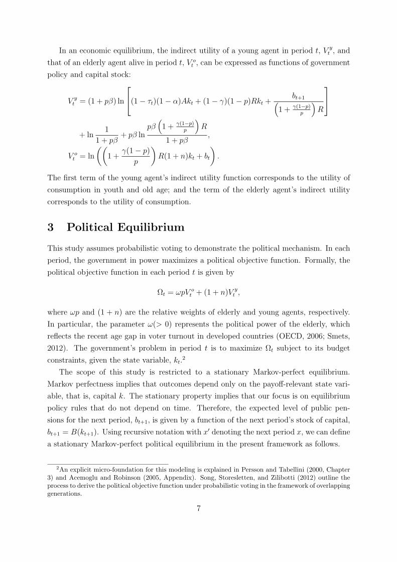
In an economic equilibrium, the indirect utility of a young agent in period t, V yt , and

that of an elderly agent alive in period t, V ot , can be expressed as functions of government

policy and capital stock:

V yt = (1 + pβ) ln

(1− τt)(1− α)Akt + (1− γ)(1− p)Rkt +bt+1(

1 + γ(1−p)p

)R

+ ln

1

1 + pβ+ pβ ln

pβ(1 + γ(1−p)

p

)R

1 + pβ,

V ot = ln

((1 +

γ(1− p)

p

)R(1 + n)kt + bt

).

The first term of the young agent’s indirect utility function corresponds to the utility of

consumption in youth and old age; and the term of the elderly agent’s indirect utility

corresponds to the utility of consumption.

3 Political Equilibrium

This study assumes probabilistic voting to demonstrate the political mechanism. In each

period, the government in power maximizes a political objective function. Formally, the

political objective function in each period t is given by

Ωt = ωpV ot + (1 + n)V y

t ,

where ωp and (1 + n) are the relative weights of elderly and young agents, respectively.

In particular, the parameter ω(> 0) represents the political power of the elderly, which

reflects the recent age gap in voter turnout in developed countries (OECD, 2006; Smets,

2012). The government’s problem in period t is to maximize Ωt subject to its budget

constraints, given the state variable, kt.2

The scope of this study is restricted to a stationary Markov-perfect equilibrium.

Markov perfectness implies that outcomes depend only on the payoff-relevant state vari-

able, that is, capital k. The stationary property implies that our focus is on equilibrium

policy rules that do not depend on time. Therefore, the expected level of public pen-

sions for the next period, bt+1, is given by a function of the next period’s stock of capital,

bt+1 = B(kt+1). Using recursive notation with x′ denoting the next period x, we can define

a stationary Markov-perfect political equilibrium in the present framework as follows.

2An explicit micro-foundation for this modeling is explained in Persson and Tabellini (2000, Chapter3) and Acemoglu and Robinson (2005, Appendix). Song, Storesletten, and Zilibotti (2012) outline theprocess to derive the political objective function under probabilistic voting in the framework of overlappinggenerations.

7

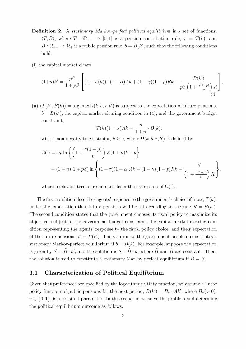
Definition 2. A stationary Markov-perfect political equilibrium is a set of functions,

⟨T,B⟩, where T : ℜ++ → [0, 1] is a pension contribution rule, τ = T (k), and

B : ℜ++ → ℜ+ is a public pension rule, b = B(k), such that the following conditions

hold:

(i) the capital market clears

(1+n)k′ =pβ

1 + pβ·

(1− T (k)) · (1− α)Ak + (1− γ)(1− p)Rk − B(k′)

pβ(1 + γ(1−p)

p

)R

,

(4)

(ii) ⟨T (k), B(k)⟩ = argmaxΩ(k, b, τ, b′) is subject to the expectation of future pensions,

b = B(k′), the capital market-clearing condition in (4), and the government budget

constraint,

T (k)(1− α)Ak =p

1 + n·B(k),

with a non-negativity constraint, b ≥ 0, where Ω(k, b, τ, b′) is defined by

Ω(·) ≡ ωp ln

(1 +

γ(1− p)

p

)R(1 + n)k + b

+ (1 + n)(1 + pβ) ln

(1− τ)(1− α)Ak + (1− γ)(1− p)Rk +b′(

1 + γ(1−p)p

)R

,

where irrelevant terms are omitted from the expression of Ω(·).

The first condition describes agents’ response to the government’s choice of a tax, T (k),

under the expectation that future pensions will be set according to the rule, b′ = B(k′).

The second condition states that the government chooses its fiscal policy to maximize its

objective, subject to the government budget constraint, the capital market-clearing con-

dition representing the agents’ response to the fiscal policy choice, and their expectation

of the future pensions, b′ = B(k′). The solution to the government problem constitutes a

stationary Markov-perfect equilibrium if b = B(k). For example, suppose the expectation

is given by b′ = B · k′, and the solution is b = B · k, where B and B are constant. Then,

the solution is said to constitute a stationary Markov-perfect equilibrium if B = B.

3.1 Characterization of Political Equilibrium

Given that preferences are specified by the logarithmic utility function, we assume a linear

policy function of public pensions for the next period, B(k′) = Bγ · Ak′, where Bγ(> 0),

γ ∈ 0, 1, is a constant parameter. In this scenario, we solve the problem and determine

the political equilibrium outcome as follows.

8

Proposition 1. There is a stationary Markov-perfect political equilibrium with b > 0 if

γ = 1 and α <1

1 + (1 + pβ)(1 + n)/ωp,

or

γ = 0 and α <1

p+ (1 + pβ)(1 + n)/ω.

For the case of b > 0 the policy function of public pensions is

BγAk =

B1Ak if γ = 1,B0Ak if γ = 0,

where

B1 ≡ω(1− α)− (1 + pβ)α

p(1 + n)

(1 + pβ) + ωp1+n

,

B0 ≡ω (1− α) + (1− p)α − (1 + pβ)α(1 + n)

(1 + pβ) + ωp1+n

(> B1) .

Proof. See Appendix A.1.

The result in Proposition 1 implies that for both cases of γ = 1 and 0, public pensions

are more likely to be provided in the political equilibrium if the political power of the

elderly (ω) is larger and/or the population growth rate (n) is lower. Greater political

power of the elderly attaches a larger weight to the utility of the elderly in the political

objective function. This incentivizes the politician to provide higher pension benefits to

the elderly. A smaller population growth rate implies lower savings per head for given

capital stock, and thus, a lower consumption level of the elderly. To maintain their

consumption level, the politician offers a larger pension benefit to the elderly.

The effects of longevity (p) on the provision of public pensions differ between the two

cases. In the presence of annuity markets (γ = 1), greater longevity has two opposing ef-

fects on pension provision. First, greater longevity leads to a lower rate of return from an-

nuity and thus, a lower consumption level in old age. To compensate for this loss of old-age

consumption, the politician offers a larger pension benefit to the elderly. This is a positive

effect on the public pension represented by the term α/p in the numerator of B1. Second,

greater longevity attaches a larger weight to the lifetime utility of the young. To improve

their utility, the politician cuts the tax burden on the young by reducing public pension

provisions for the elderly. This is a negative effect on the public pension represented

by the term pβ on the numerator of B1. The condition α < [1 + (1 + pβ)(1 + n)/ωp]−1

implies that the former positive effect outweighs the latter negative effect when γ = 1.

In the absence of annuity markets (γ = 0), the negative effect remains, but the positive

effect through the annuity returns disappears. Instead, there is an additional negative

effect through the accidental bequest represented by the term (1− p)α in the numerator

9

of B0. That is, an increase in longevity decreases the accidental bequests and thereby

creates a negative income effect on the young. This negative effect, accompanied with the

negative effect that remains in the absence of annuity markets, incentivizes the politician

to cut the tax burden on the young and thereby to reduce the pension benefit to the

elderly. Therefore, in the absence of annuity markets, public pensions are less likely to be

provided if longevity is higher.

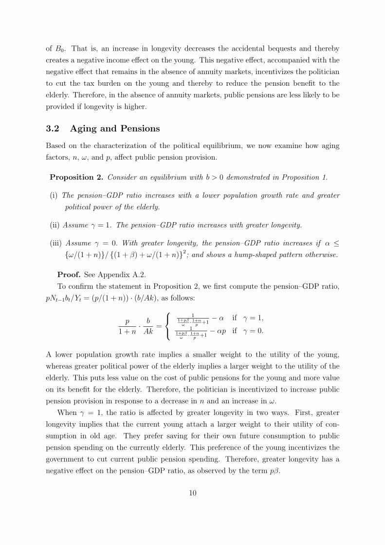
3.2 Aging and Pensions

Based on the characterization of the political equilibrium, we now examine how aging

factors, n, ω, and p, affect public pension provision.

Proposition 2. Consider an equilibrium with b > 0 demonstrated in Proposition 1.

(i) The pension–GDP ratio increases with a lower population growth rate and greater

political power of the elderly.

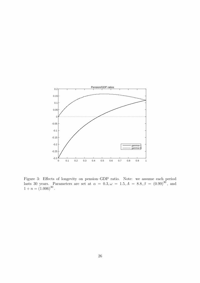
(ii) Assume γ = 1. The pension–GDP ratio increases with greater longevity.

(iii) Assume γ = 0. With greater longevity, the pension–GDP ratio increases if α ≤ω/(1 + n)/ (1 + β) + ω/(1 + n)2; and shows a hump-shaped pattern otherwise.

Proof. See Appendix A.2.

To confirm the statement in Proposition 2, we first compute the pension–GDP ratio,

pNt−1bt/Yt = (p/(1 + n)) · (b/Ak), as follows:

p

1 + n· b

Ak=

1

1+pβω

· 1+np

+1− α if γ = 1,

11+pβ

ω· 1+n

p+1

− αp if γ = 0.

A lower population growth rate implies a smaller weight to the utility of the young,

whereas greater political power of the elderly implies a larger weight to the utility of the

elderly. This puts less value on the cost of public pensions for the young and more value

on its benefit for the elderly. Therefore, the politician is incentivized to increase public

pension provision in response to a decrease in n and an increase in ω.

When γ = 1, the ratio is affected by greater longevity in two ways. First, greater

longevity implies that the current young attach a larger weight to their utility of con-

sumption in old age. They prefer saving for their own future consumption to public

pension spending on the currently elderly. This preference of the young incentivizes the

government to cut current public pension spending. Therefore, greater longevity has a

negative effect on the pension–GDP ratio, as observed by the term pβ.

10

Second, greater longevity leads to a higher dependency ratio, and thereby a higher

pension–GDP ratio. This positive effect is observed by the term (1 + n)/p. Therefore,

greater longevity has two opposing effects on the ratio, but the result in Proposition

1(ii) shows that the latter always outweighs the former in the political equilibrium if

γ = 1. This result is consistent with the prediction of Gonzalez-Eiras and Niepelt’s

(2008) model using a neoclassical growth framework. The present analysis indicates that

their prediction also holds in an endogenous growth model with AK technology. The solid

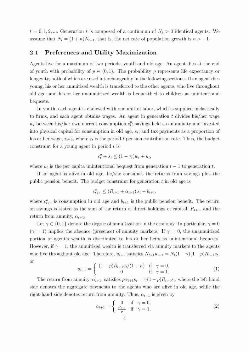
curve in Figure 3 illustrates a numerical example of the ratio when γ = 1.

[Figure 3 here.]

When γ = 0, there is an additional negative effect represented by the term αp. Greater

longevity implies that more weight is attached to the return from savings; agents increase

savings as longevity increases. The politician takes account of this economic behavior in

policy decision making, and given that savings are perfectly substitutable with pensions,

he or she offers lower pension benefits as longevity increases. When γ = 1, this negative

effect on pension is offset by the decrease in the return from annuity, R = R/p. However,

there is no such cancellation effect when γ = 0.

The term αp, representing the aforementioned negative effect, becomes larger as the

interest rate, R = αA, increases. In particular, if α is small, such that α ≤ ω/(1 +

n)/ (1 + β) + ω/(1 + n)2, the sum of the negative effects is outweighed by the positive

effect; greater longevity leads to a higher pension–GDP ratio. However, if α is above the

critical value, an increase in longevity produces an initial increase followed by a decrease

in the ratio. The dotted curve in Figure 3 illustrates a numerical example of the hump-

shaped pattern of the ratio when γ = 0.

To recap, the pension–GDP ratio increases as longevity rises in the presence of an

annuity market. In its absence, the ratio increases or exhibits a hump-shaped pattern as

longevity rises. These different effects of longevity could be ascribed to the presence (or

absence) of annuities. Therefore, the extent of annuitization may be an important feature

in providing an explanation for the mixed evidence on the pension–GDP ratio observed

for high-longevity countries in Figure 1.

3.3 Aging and Economic Growth

The result in Proposition 1 enables us to derive the growth rate of per capita capital, k′/k,

and to investigate how the growth rate is affected by population aging. The following

proposition summarizes the result.

Proposition 3. Consider an equilibrium with b > 0.

11

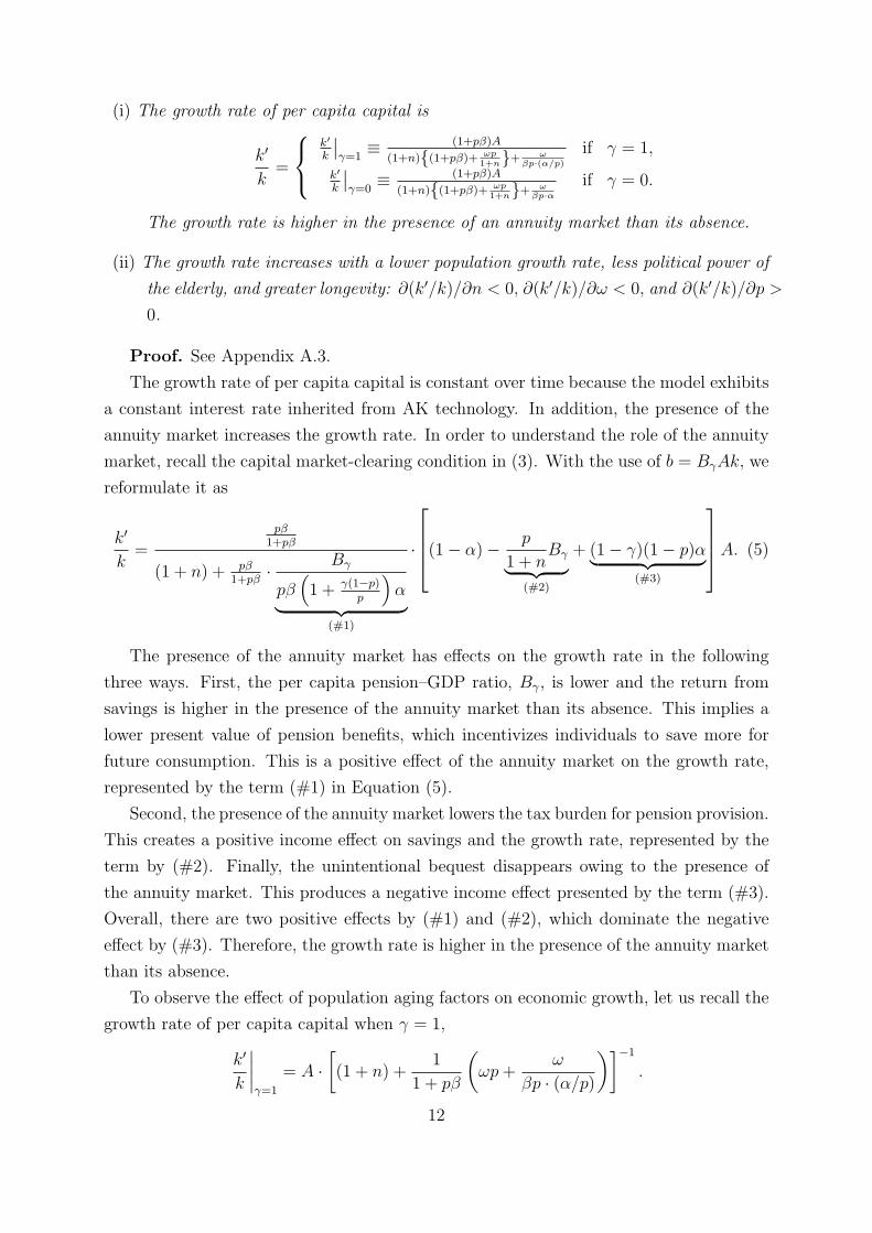
(i) The growth rate of per capita capital is

k′

k=

k′

k

∣∣γ=1

≡ (1+pβ)A

(1+n)(1+pβ)+ ωp1+n+ ω

βp·(α/p)

if γ = 1,

k′

k

∣∣γ=0

≡ (1+pβ)A

(1+n)(1+pβ)+ ωp1+n+ ω

βp·αif γ = 0.

The growth rate is higher in the presence of an annuity market than its absence.

(ii) The growth rate increases with a lower population growth rate, less political power of

the elderly, and greater longevity: ∂(k′/k)/∂n < 0, ∂(k′/k)/∂ω < 0, and ∂(k′/k)/∂p >

0.

Proof. See Appendix A.3.

The growth rate of per capita capital is constant over time because the model exhibits

a constant interest rate inherited from AK technology. In addition, the presence of the

annuity market increases the growth rate. In order to understand the role of the annuity

market, recall the capital market-clearing condition in (3). With the use of b = BγAk, we

reformulate it as

k′

k=

pβ1+pβ

(1 + n) + pβ1+pβ

· Bγ

pβ(1 + γ(1−p)

p

)α︸ ︷︷ ︸

(#1)

·

(1− α)− p

1 + nBγ︸ ︷︷ ︸

(#2)

+ (1− γ)(1− p)α︸ ︷︷ ︸(#3)

A. (5)

The presence of the annuity market has effects on the growth rate in the following

three ways. First, the per capita pension–GDP ratio, Bγ, is lower and the return from

savings is higher in the presence of the annuity market than its absence. This implies a

lower present value of pension benefits, which incentivizes individuals to save more for

future consumption. This is a positive effect of the annuity market on the growth rate,

represented by the term (#1) in Equation (5).

Second, the presence of the annuity market lowers the tax burden for pension provision.

This creates a positive income effect on savings and the growth rate, represented by the

term by (#2). Finally, the unintentional bequest disappears owing to the presence of

the annuity market. This produces a negative income effect presented by the term (#3).

Overall, there are two positive effects by (#1) and (#2), which dominate the negative

effect by (#3). Therefore, the growth rate is higher in the presence of the annuity market

than its absence.

To observe the effect of population aging factors on economic growth, let us recall the

growth rate of per capita capital when γ = 1,

k′

k

∣∣∣∣γ=1

= A ·[(1 + n) +

1

1 + pβ

(ωp+

ω

βp · (α/p)

)]−1

.

12

Thus, the growth rate is affected by population aging via the terms, (1 + n), 1 + pβ, ωp,

and ω/ (βp · (α/p)). When γ = 0, the term ω/ (βp · (α/p)) is replaced by ω/ (βpα).

Population growth, the political power of the old, and longevity have the following

implications for economic growth via these terms. First, a lower population growth rate

increases per capita capital equipment in the economy. This effect, which is observed

by the term (1 + n), accelerates capital accumulation and economic growth. Second,

greater political power of the elderly attaches a larger weight to the utility of the current

elderly. This incentivizes the government to increase the public pension expenditure,

thereby resulting in a greater tax burden on the young. This effect, which is observed

by the terms ωp and ω/ (βp · (α/p)), discourages saving of the young and thus, impedes

economic growth.

Greater longevity has the following effects on the growth rate via the terms 1 + pβ,

ωp, and ω/ (βp · (α/p)) when γ = 1. First, greater longevity attaches a larger weight to

the lifetime utility of the young as represented by the term pβ. The young save more

for their consumption in old age in response to an increase in longevity. This creates a

positive effect on economic growth. Second, greater longevity attaches a larger weight to

the utility of the elderly, too. As described earlier in this subsection, this increases the

tax burden on the young and thus, has a negative effect on economic growth.

Third, greater longevity lowers the rate of return from annuity, R = R/p, and thus,

increases the present value of public pension benefits. In response to this increase, individ-

uals save less because pension benefits are perfect substitutes for savings. This negative

effect on economic growth is observed in the term ω/ (βp · (α/p)) and is peculiar to the

case of γ = 1. Thus far, the three effects imply that longevity has mixed growth effects,

but the net effect is positive when γ = 1. The result is qualitatively unchanged when

γ = 0 because the last negative effect disappears.

The model prediction regarding population growth is consistent with the observation

in Panel (a) of Figure 2, but the prediction regarding longevity is inconsistent with the

observation in Panel (b); the evidence shows that higher life expectancy results in a

lower growth rate. This inconsistency is resolved when we focus on another aging factor,

that is, the political power of the elderly. Greater longevity implies a larger share of

the elderly in the population, which might, in turn, lead to larger political power of the

elderly (OECD, 2006; Smets, 2012). Given the negative effect of the power on economic

growth, we might argue that the negative correlation between life expectancy and per

capita economic growth observed in Panel (b) of Figure 2 could be explained when the

effects of longevity and the political power of the elderly are examined together.

13

3.4 Welfare Analysis

The previous subsection shows that the growth rate is higher in the presence of the annuity

market than in its absence. A higher growth rate generates more resources available

for future generations. This implies that future generations are made better off by the

presence of the annuity market. However, the presence of the annuity market increases

the rate of return from saving and thus, lowers the present value of public pensions. This

works to decrease the present value of lifetime income and consumption. Hence, it may

be possible that the present generation is made worse off by the presence of the annuity

market compared to its absence.

In order to investigate such a possibility, we compare the indirect utility functions

when γ = 1 and γ = 0 for a given k as follows:

V y|γ=1 ≷ V y|γ=0

⇔ pβ ln(1/p) + (1 + pβ) ln p+ (1 + pβ) ln(k′/k|γ=1

)t

≷ (1 + pβ) ln(k′/k|γ=0

)t

.

(6)

From this condition, we obtain the following result.

Proposition 4. Consider an equilibrium with b > 0.

(i) For generation 0, the expected utility of the young is higher in the absence of the

annuity market than its presence.

(ii) Along the equilibrium path with k′/k > 1, there is some T (> 1) such that the expected

utility of generation t(≥ T ) is higher in the presence of the annuity market than its

absence.

Proof. See Appendix A.4.

To understand the argument in Proposition 4, let us look at the condition in (6). The

first term on the left-hand side, pβ ln(1/p), shows a positive effect of the annuity market.

The presence of the annuity market increases the return from saving, which works to

increase the old-age consumption. However, an increase in the interest rate lowers the

present value of public pension benefits. This works to decrease lifetime consumption

and thereby creates a negative effect on utility. This negative effect is represented by the

second term on the left-hand side, denoted by (1 + pβ) ln p. The net effect of these two

opposing effects through the interest rate is negative.

The third term on the left-hand side, (1+pβ) ln(k′/k|γ=1

)t

, and the term on the right-

hand side, (1 + pβ) ln(k′/k|γ=0

)t

, show the lifetime income (i.e., lifetime consumption)

that is affected by the growth rate. Given the result in Proposition 3, we find that the

14

lifetime income when γ = 1 is larger than that when γ = 0. The growth effect works

from generation 1 onward, and the difference in the lifetime income becomes larger as

time passes.

Overall, the presence of the annuity market creates a negative effect through the

interest rate and a positive effect through the growth rate. For generation 0, the growth

effect is irrelevant, and thus, it is made better off in the absence of the annuity market

compared to its absence. However, from generation 1 onward, the positive growth effect

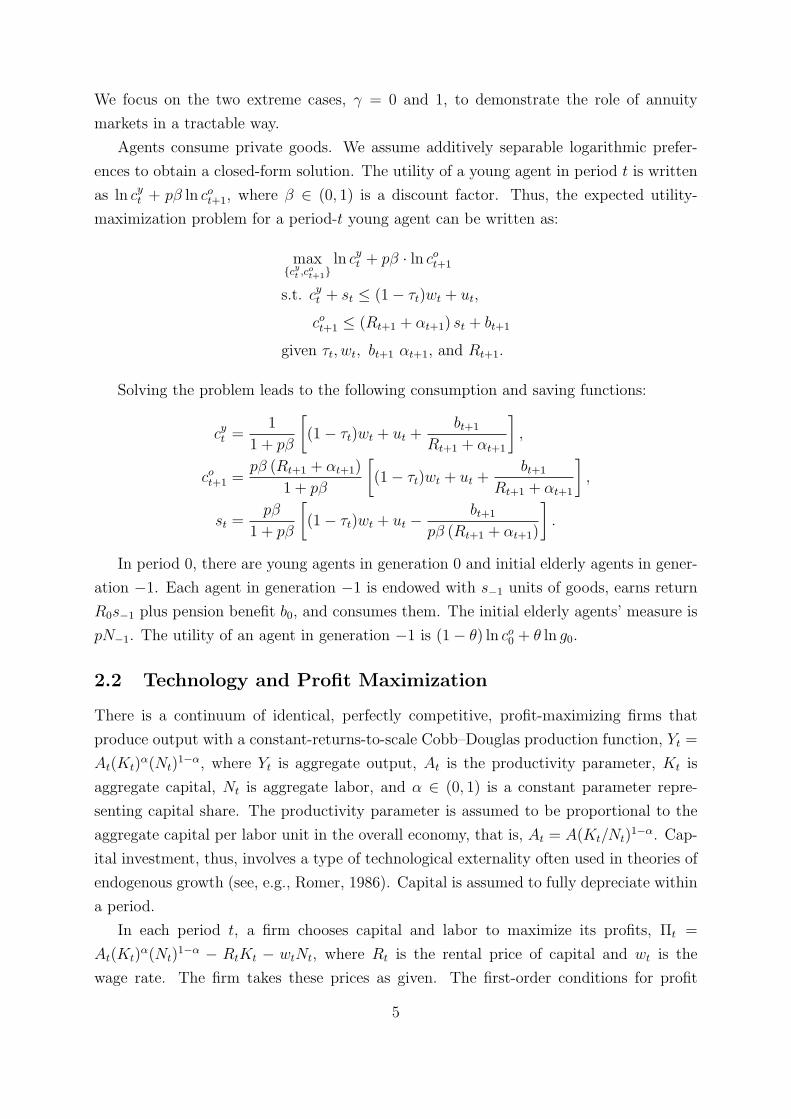
is relevant, and this effect becomes larger as time passes. Therefore, there is some T (> 0)

such that the expected utility of generation t(≥ T ) is higher in the presence of the annuity

market than its absence. A numerical example is demonstrated in Figure 4.

[Figure 4 here.]

3.5 Alternative Production Function

In previous subsections, we conduct the analysis by assuming AK technology that exhibits

a constant interest rate. Within this assumption, we show that the pension–GDP ratio

increases with longevity in the presence of an annuity market, while it may show a hump-

shaped pattern in the absence of the market. In other words, greater longevity is less

likely to increase the pension–GDP ratio in the absence of the annuity market compared

to in the presence of the annuity market.

In order to investigate whether this result still holds when the interest rate is endoge-

nous, we here undertake a brief analysis by alternatively assuming a neoclassical produc-

tion function, yt = A (kt)α. The interest rate and wage are given by Rt = αA (kt)

α−1 and

wt = (1− α)A (kt)α , respectively. The interest rate is now decreasing in capital.

The indirect utility function of the young is

V y = (1 + pβ) ln

(1− α)A (k)α + (1− γ)(1− p)αA (k)α +b′(

1 + γ(1−p)p

)αA (k′)α−1

+ pβ ln

(1/ (k′)

1−α),

where the second term on the right-hand side, representing the utility of the return from

saving, indicates that the choice of public pension affects the lifetime utility of the young

through the interest rate. This effect is not included in the model with AK technology.

Following the procedure in Subsection 3.1, we guess that the future public pension is

given by b′ = B0 ·A (k′)α . Given this guess and the capital market-clearing condition, the

term pβ ln(1/ (k′)1−α) is reformulated as

pβ ln(1/ (k′)

1−α)= pβ ln

[1

(1− α) + (1− γ)(1− p)α− p1+n

· bA(k)α

].

15

The expression suggests that a higher pension–GDP ratio, (p/(1 + n)) · (b/A (k)α), is

associated with lower capital in the next period and thereby a higher interest rate.

The expression shows that longevity has two additional effects on the pension–GDP

ratio, (p/(1 + n)) · (b/A (k)α), through the terms pβ and (1− γ)(1− p)α. First, the term

pβ indicates that greater longevity attaches a larger weight to the utility of the interest

rate and thereby works to increase the pension–GDP ratio. This positive effect appears

for both cases. Second, the term (1 − γ)(1 − p)α shows that greater longevity reduces

the unintentional bequests. To compensate for this loss of bequests, the government may

attempt to lower the pension–GDP ratio. This negative effect, peculiar to the case of no

annuity market, implies that greater longevity is less likely to increase the pension–GDP

ratio in the absence of the annuity market compared to its presence. This property is

qualitatively equivalent to that in the model with AK technology.

4 Concluding Remarks

This study attempted to examine how an aging population affects voting on pension

expenditure, and how this expenditure in turn affects economic growth. To address these

issues, we used an endogenous growth, overlapping-generation model in which pension

expenditure is financed by tax on the working young. The expenditure is determined via

probabilistic voting that captures the intergenerational conflict caused by the three factors

of population aging—a decline in the population growth rate, a rise in life expectancy,

and an increase in the political power of the elderly.

We considered two alternative cases, in which an annuity market is either present

or absent, and showed the following. First, the pension–GDP ratio increases as life ex-

pectancy increases in the presence of the annuity market. However, the ratio may show

a hump-shaped pattern in the absence of the annuity market. Second, the growth rate is

increased by a lower population growth rate, less political power of the elderly, and greater

longevity. However, when the longevity and political power of the elderly are examined

together, greater longevity could be associated with a lower growth rate. These results

are consistent with the observed evidence in OECD countries.

To evaluate the role of the annuity market, we compared the two cases, the presence

and absence of the annuity market, in terms of growth and welfare. We showed that (i)

the growth rate is higher in the presence of the annuity market than its absence; and (ii)

due to this growth effect, future generations are made better off by the presence of the

annuity market, but the current generation cannot benefit from future growth. These

results suggest that the development of annuity markets is beneficial from the viewpoint

of economic growth, but implies an intergenerational trade-off in terms of utility.

16

A Proofs

A.1 Proof of Proposition 1

Suppose that public pensions are provided in equilibrium in the next period, b′ > 0.

Assume a linear policy function of public pensions for the next period, B(k′) = BγAk′,

where Bγ(> 0) is a constant parameter. Given this assumption and the government

budget constraint, the capital market-clearing condition in Definition 2 becomes

(1+n)k′ =pβ

1 + pβ·

(1− α)Ak − p

1 + nB(k) + (1− γ)(1− p)Rk − BγAk

′

pβ(1 + γ(1−p)

p

)R

,

which is rewritten as

k′ =

pβ1+pβ

(1 + n) + pβ1+pβ

· BγA

pβ(1+ γ(1−p)p )R

·[(1− α)Ak − p

1 + nB(k) + (1− γ)(1− p)Rk

]. (7)

Using (7) and the assumption B(k′) = BAk′, we write the present value of lifetime

income as

(1− α)Ak − p

1 + nB(k) + (1− γ)(1− p)Rk +

BγA(1 + γ(1−p)

p

)Rk′

=

1 + BγA(1 + γ(1−p)

p

)R

·pβ

1+pβ

(1 + n) + pβ1+pβ

· BγA

pβ(1+ γ(1−p)p )R

×[(1− α)Ak − p

1 + nB(k) + (1− γ)(1− p)Rk

]. (8)

Equations (7) and (8) enable us to write the political objective function as follows:

Ω = ωp ln

((1 +

γ(1− p)

p

)R(1 + n)k +B(k)

)+ (1 + n) (1 + pβ) ln

[(1− α)Ak − p

1 + nB(k) + (1− γ)(1− p)Rk

],

where the terms unrelated to political decisions are omitted from the expression.

The first-order condition with respect to B(k) is given by

B(k) :ωp(

1 + γ(1−p)p

)R(1 + n)k +B(k)

=(1 + n)(1 + pβ) p

1+n

(1− α)Ak − p1+n

B(k) + (1− γ)(1− p)Rk.

Recalling that R = αA, this expression is reduced to

B(k) =ω (1− α) + (1− γ)(1− p)α − (1 + pβ)

(1 + γ(1−p)

p

)α(1 + n)

(1 + pβ) + ωp1+n

· Ak,

17

or,

B(k) =

Bγ=1Ak if γ = 1,Bγ=0Ak if γ = 0,

where Bγ=1 and Bγ=0 are defined by

Bγ=1 ≡ω(1− α)− (1 + pβ)α

p(1 + n)

(1 + pβ) + ωp1+n

,

Bγ=0 ≡ω (1− α) + (1− p)α − (1 + pβ)α(1 + n)

(1 + pβ) + ωp1+n

.

Therefore, we obtain b > 0 if

Bγ=1 > 0 ⇔ ω >α(1 + pβ)(1 + n)

(1− α)pwhen γ = 1,

Bγ=0 > 0 ⇔ ω >α(1 + pβ)(1 + n)

(1− α) + (1− p)αwhen γ = 0.

A.2 Proof of Proposition 2

Using the policy function B(·) in Proposition 1, the pension–GDP ratio, pNt−1bt/Yt =

(p/(1 + n)) · (b/Ak), is computed as follows:

p

1 + n· b

Ak=

p

1+n· ω−αω+(1+pβ)(1+n)/p

(1+pβ)+ωp/(1+n)if γ = 1,

p1+n

· ω−αpω+(1+pβ)(1+n)(1+pβ)+ωp/(1+n)

if γ = 0.

That is,

p

1 + n· b

Ak=

1

(1+pβ)(1+n)ωp

+1− α if γ = 1,

1(1+pβ)(1+n)

ωp+1

− αp if γ = 0.

This expression shows that the ratio is decreasing in n and increasing in ω. In addition,

the ratio is increasing in p if γ = 1.

To determine the effect of p when γ = 0, we take the first- and second-order differen-

tiations with respect to p and obtain

∂

[p

1 + n· b

Ak

∣∣∣∣γ=0

]/∂p =

ω(1 + n)

[(1 + pβ)(1 + n) + ωp]2− α,

∂2

[p

1 + n· b

Ak

∣∣∣∣γ=0

]/∂p2 < 0.

The ratio is strictly concave in p with

∂

[p

1 + n· b

Ak

∣∣∣∣γ=0

]/∂p

∣∣∣∣∣p=0

=ω

1 + n− α,

∂

[p

1 + n· b

Ak

∣∣∣∣γ=0

]/∂p

∣∣∣∣∣p=1

=ω/(1 + n)

(1 + β) + ω/(1 + n)2− α.

18

The result suggests that there are two threshold values of α, ω/(1 + n) and ω/(1 +

n) (1 + β) + ω/(1 + n)2, such that

∂

[p

1 + n· b

Ak

∣∣∣∣γ=0

]/∂p < 0∀p ∈ (0, 1) if

ω

1 + n≤ α,

∂

[p

1 + n· b

Ak

∣∣∣∣γ=0

]/∂p > 0∀p ∈ (0, 1) if

ω/(1 + n)

(1 + β) + ω/(1 + n)2≥ α.

Recall that when γ = 0, b > 0 holds if α < [p+ (1 + pβ)(1 + n)/ω]−1 (Proposition 1).

After some manipulation, we find that the following relation holds:

ω/(1 + n)

(1 + β) + ω/(1 + n)2<

1

p+ (1 + pβ)(1 + n)/ω<

ω

1 + n.

This relation indicates that the threshold value ω/(1+n) is irrelevant for the current case.

Therefore, we can conclude that

∂

[p

1 + n· b

Ak

∣∣∣∣γ=0

]/∂p > 0∀p ∈ (0, 1) if α ≤ ω/(1 + n)

(1 + β) + ω/(1 + n)2,

∂

[p

1 + n· b

Ak

∣∣∣∣γ=0

]/∂p

∣∣∣∣∣p=0

> 0 and ∂

[p

1 + n· b

Ak

∣∣∣∣γ=0

]/∂p

∣∣∣∣∣p=1

< 0

ifω/(1 + n)

(1 + β) + ω/(1 + n)2< α <

1

p+ (1 + pβ)(1 + n)/ω.

A.3 Proof of Proposition 3

(i) Recall the capital market-clearing condition in Definition 1. With the use of the

government budget constraint, τ(1−α)Ak = pb/(1+ n), the condition is reformulated as

k′ =

pβ1+pβ

(1 + n) + pβ1+pβ

· Bγ

pβ(1+ γ(1−p)p )α

·[(1− α)Ak − p

1 + nB(k) + (1− γ)(1− p)αAk

].

Substituting the policy function derived in Proposition 1, we reformulate the above ex-

pression as presented in Proposition 3(i). Direct comparison leads to k′/k|γ=1 > k′/k|γ=0.

(ii) The expressions in Proposition 3(i) indicate that

∂ k′/k|γ=1 /∂ω < 0, ∂ k′/k|γ=1 /∂n < 0,

∂ k′/k|γ=0 /∂ω < 0, ∂ k′/k|γ=0 /∂n < 0.

19

To find the effect of p, we first reformulate the expressions as

k′

k

∣∣∣∣γ=1

= A ·[(1 + n) +

ω

1 + pβ

(p+

1

βα

)]−1

, (9)

k′

k

∣∣∣∣γ=1

= A ·[(1 + n) +

ω

1 + pβ

(p+

1

pβα

)]−1

. (10)

The differentiation of the term ω1+pβ

(p+ 1

βα

)in (9) with respect to p is

∂

ω

1 + pβ

(p+

1

βα

)/∂p =

1

(1 + pβ)2

(1− p(1− β)− 1

βα

)< 0.

The differentiation of the term ω1+pβ

(p+ 1

pβα

)in (10) with respect to p is

∂

ω

1 + pβ

(p+

1

pβα

)/∂p =

1

(1 + pβ)2

(1− 1

βαp2− 2

αp

)< 0.

Therefore, ∂ k′/k|γ /∂p > 0 holds for both cases.

A.4 Proof of Proposition 4

Let V y|γ=1 and V y|γ=0 denote the lifetime utility functions of the young when γ = 1 and

γ = 0, respectively. For a given k, the functions are

V y|γ=1 = (1 + pβ) ln

[(1− α)Ak − p

1 + nBγ=1Ak

]+ (1 + pβ) ln

Bγ=1

α/p·

pβ1+pβ

(1 + n) + pβ1+pβ

· Bγ=1

pβα/p

+ ln1

1 + pβ+ pβ ln

pβ

1 + pβ· αpA,

V y|γ=0 = (1 + pβ) ln

[(1− α)Ak − p

1 + nBγ=0Ak + (1− p)αAk

]+

(1 + pβ) lnBγ=0

α·

pβ1+pβ

(1 + n) + pβ1+pβ

· Bγ=0

pβα

+ ln1

1 + pβ+ pβ ln

pβ

1 + pβ· αA.

We first reformulate the first term in each expression as follows:

(1 + pβ) ln

[(1− α)Ak − p

1 + nBγ=1Ak

]= (1 + pβ) ln

1 + pβ

(1 + pβ) + ωp1+n

A(k′/k|γ=1

)t

k0,

(1 + pβ) ln

[(1− α)Ak − p

1 + nBγ=0Ak + (1− p)αAk

]= (1 + pβ) ln

1 + pβ

(1 + pβ) + ωp1+n

A(k′/k|γ=0

)t

k0.

Second, we compare the second term in each expression and obtain

(1 + pβ) lnBγ=1

α/p·

pβ1+pβ

(1 + n) + pβ1+pβ

· Bγ=1

pβα/p

≷ (1 + pβ) lnBγ=0

α·

pβ1+pβ

(1 + n) + pβ1+pβ

· Bγ=0

pβα

⇔ (1 + pβ) ln p ≷ (1 + pβ) ln 1 = 0.

20

Given the result thus far, we obtain

V y|γ=1 ≷ V y|γ=0 ⇔ (1 + pβ) ln(k′/k|γ=1

)t

+ pβ ln(1/p) + (1 + pβ) ln p ≷ (1 + pβ) ln(k′/k|γ=0

)t

⇔ (1 + pβ) ln(k′/k|γ=1

)t

+ ln p ≷ (1 + pβ) ln(k′/k|γ=0

)t

.

If t = 0, then we obtain V y|γ=1 < V y|γ=0 because ln p < 0. For t ≥ 1, k′/k|γ=1 > k′/k|γ=0

holds, as demonstrated in Proposition 3. Therefore, there is some T (> 1) such that

V y|γ=1 > V y|γ=0 for t ≥ T .

21

References[1] Abel, A.B., 1985. Precautionary saving and accidental bequests. American Economic Re-

view 75, 777–791.

[2] Acemoglu, D., and Robinson, J.A., 2005. Economic Origins of Dictatorship and Democracy,Cambridge University Press.

[3] Azariadis, C., and Galasso, V., 2002. Fiscal constitutions. Journal of Economic Theory 103,255–281.

[4] Bassetto, M., 2008. Political economy of taxation in an overlapping-generations economy.Review of Economic Dynamics 11, 18–43.

[5] Boldrin, M., and Rustichini, A., 2000. Political equilibria with social security. Review ofEconomic Dynamics 3, 41–78.

[6] Chen, K., and Song, Z., 2014. Markovian social security in unequal societies. ScandinavianJournal of Economics 116, 982–1011.

[7] Cooley, T.F., and Soares, J., 1999. A positive theory of social security based on reputation.Journal of Political Economy 107, 135–160.

[8] Forni, L., 2005. Social security as Markov equilibrium in OLG models. Review of EconomicDynamics 8, 178–194.

[9] Gonzalez-Eiras, M., and Niepelt, D., 2008. The future of social security. Journal of MonetaryEconomics 55, 197–218.

[10] Gonzalez-Eiras, M., and Niepelt, D., 2012. Ageing, government budgets, retirement, andgrowth. European Economic Review 56, 97–115.

[11] Gradstein, M., and Kaganovich, M., 2004. Aging population and education finance. Journalof Public Economics 88, 2469–2485.

[12] Grossman, G., and Helpman, E., 1998. Intergenerational redistribution with short-livedgovernments. Economic Journal 108, 1299–1329.

[13] Kunze, L., 2014. Life expectancy and economic growth. Journal of Macroeconomics 39,Part A, 54–65.

[14] Lancia, F., and Russo, A., 2015. Public education and pensions in democracy:a political economic theory. http://www.sv.uio.no/econ/english/research/unpublished-works/working-papers/pdf-files/2015/memo-01-2015.pdf (August 25, 2015).

[15] Lindbeck, A., and Weibull, J., 1987. Balanced budget redistribution and the outcome ofpolitical competition. Public Choice 52, 273–297.

[16] Mateos-Planas, X., 2008. A quantitative theory of social security without commitment.Journal of Public Economics 92, 652–671.

[17] OECD, 2006. Society at a Glance: OECD Social Indicators-2006 Edition. OECD Publish-ing.

[18] OECD, 2011. OECD Factbook 2011-2012: Economic, Environmental and Social Statistics.OECD Publishing.

[19] Ono, T., and Uchida, Y., 2016. Pensions, education, and growth: a positive analysis. Journalof Macroeconomics 48, 127–143.

[20] Persson, T., and Tabellini, G., 2000. Political Economics: Explaining Economic Policy.MIT Press.

22

[21] Romer, Paul M., 1986. Increasing returns and long run growth. Journal of Political Economy94, 1002–1037.

[22] Rusconi, R., 2008. National annuity markets; features and implications. OECD WorkingPapers on Insurance and Private Pensions, No. 24. OECD Publishing.

[23] Sheshinski, E., and Weiss, Y., 1981. Uncertainty and optimal social security systems. Quar-terly Journal of Economics 96, 189–206.

[24] Smets, K., 2012. A widening generational divide? The age gap in voter turnout throughtime and space. Journal of Elections, Public Opinion and Parties 22, 407–430.

[25] Song, Z., Storesletten, K., and Zilibotti, F., 2012. Rotten parents and disciplined children:a politico-economic theory of public expenditure and debt. Econometrica 80, 2785–2803.

[26] Zhang, J., Zhang, J., and Lee, R., 2003. Rising longevity, education, savings, and growth.Journal of Development Economics 70, 83–101.

23

AUS

AUT

BEL

CANCHL

CZE

DNKEST

FIN

FRA

DEUGRC

HUN

ISLIRL

ISR

ITA

JPN

KOR

LUX

MEX

NLDNZLNOR

POL

PRT

SVK

SVNESP

SWECHE

TUR

GBR

USA

0

2

4

6

8

10

12

-2 -1 0 1 2 3 4

pe

nsi

on

-GD

P r

a!

o a

ve

rag

e 2

00

1-2

01

0

popula!on growth rate average 1991-2000

popula!on growth and pension-GDP ra!o

(a)

AUS

AUT

BEL

CANCHL

CZE

DNKEST

FIN

FRA

DEUGRC

HUN

ISLIRL

ISR

ITA

JPN

KOR

LUX

MEX

NLDNZLNOR

POL

PRT

SVK

SVNESP

SWECHE

TUR

GBR

USA

0

2

4

6

8

10

12

14 15 16 17 18 19 20 21

pe

nsi

on

-GD

P r

a!

o a

ve

rag

e 2

00

1-2

01

0

males' life expectancy at 60 averagea 1991-2000

life expectancy and pension-GDP ra!o

(b)

Figure 1: Panel (a): The relationship between average pension–GDP ratio, 2001–2010, and average population growth rate, 1991–2000, for OECD countries. Panel(b): The relationship between average pension–GDP ratio, 2001–2010, and averagemale life expectancy at 60 years, 1991–2000, for OECD countries. Source: OECD.Stat(http://stats.oecd.org/).

24

AUSAUTBEL CAN

CHLCZE

DNK

EST

FIN

FRA

DEUGRC

HUN

ISLIRL ISR

ITA

JPN

KOR

LUX

MEXNLD

NZL

NOR

POL

PRT

SVK

SVN

ESP

SWE

CHE

TUR

GBRUSA

-1

0

1

2

3

4

5

6

-2 -1 0 1 2 3 4

pe

r ca

pit

a G

DP

gro

wth

ave

rag

e 1

99

1-

20

00

popula!on growth average 1991-2000

popula!on growth and per capita GDP growth

(a)

AUSAUTBELCAN

CHLCZE

DNK

EST

FIN

FRA

DEUGRC

HUN

ISLIRL ISR

ITA

JPN

KOR

LUX

MEXNLD

NZL

NOR

POL

PRT

SVK

SVN

ESP

SWE

CHE

TUR

GBRUSA

-1

0

1

2

3

4

5

6

14 15 16 17 18 19 20 21

pe

r ca

pit

a g

row

th a

ve

rag

e 2

00

1-2

01

0

males life expectancy at 60 average 1991-2000

life expectancy and per capita growth

(b)

Figure 2: Panel (a): The relationship between average per capita growth, 2001–2010, andaverage population growth rate, 1991–2000, for OECD countries. Panel (b): The relation-ship between average per capita growth, 2001–2010, and average male life expectancy at60 years, 1991–2000, for OECD countries. Source: OECD.Stat (http://stats.oecd.org/).

25

0 0.1 0.2 0.3 0.4 0.5 0.6 0.7 0.8 0.9 1-0.3

-0.25

-0.2

-0.15

-0.1

-0.05

0

0.05

0.1

0.15

0.2Pension/GDP ratios

gamma=1gamma=0

Figure 3: Effects of longevity on pension–GDP ratio. Note: we assume each periodlasts 30 years. Parameters are set at α = 0.3, ω = 1.5, A = 8.8, β = (0.99)30 , and1 + n = (1.006)30 .

26

0 0.5 1 1.5 2 2.5 3 3.5 4 4.5 5-2

-1.5

-1

-0.5

0

0.5

1

1.5

2expected utility of the young, from generation 0 to generation 5

gamma=1gamma=0

Figure 4: Expected lifetime utility of the young from generation 0 to generation 5. Note:parameters are set at α = 0.3, ω = 1.5, A = 8.8, p = 0.7, β = (0.99)30 , and 1 + n =(1.006)30 . The initial condition is k0 = 1.

27