Embed Size (px)
Citation preview

DISSERATATION
Titel der DissertationMerging GW with DMFT
VerfasserMag. Merzuk Kaltak
angestrebter akademischer GradDoktor der Naturwissenschaften (Dr. rer. nat.)
Wien, 2015
Sudienkennzahl lt. Studienblatt: A 791 411Dissertationsgebiet lt. Studienblatt: PhysikBetreuerin / Betreuer: Univ.-Prof. Dipl.-Ing. Dr. Georg Kresse


Vorwort
Die vorliegende Arbeit besteht aus zwei Teilen. Der erste Teil deckt im
wesentlichen Literatur von Vielelektronensystemen in kondensierter Materie
ab und fasst alle theoretischen Grundlagen zusammen, die notwendig sind um
die GW -Naherung der Schwinger-Dyson-Gleichungen mit der Dynamischen
Molekularfeldtheorie (DMFT) zu kombinieren. Die Vereinigung von GW mit
DMFT (besprochen in Kapitel 4) ist theoretisch anspruchsvoll und benotigt
eine detailierte Einfuhrung in die diagramatische Storungstheorie (Kapitel 2
und 3) , um eine konsistente Therminologie fur das Verstandnis des zweiten
Teils der vorliegenden Disseratation aufzubauen.
Der zweite Teil der vorliegenden Arbeit beinhaltet zwei Kapitel die aus
einer Kollektion von kurzlich publizierten Arbeiten bestehen. Darin werden
methodologische Entwicklungen fur das Ausfuhren von praktischen GW+
DMFT-Rechnungen vorgestellt beginnend mit einem effizienten Algorithmus
fur die Berechnung der elektronischen Korrelationsenergie in der Random-
Phase-Approximation (RPA) in Kapitel 5. Da die GW -Naherung mit der
RPA eng verwandt ist, kann der prasentierte RPA-Algorithmus als der erste
Schritt zu einem effizienten GW -Algorithmus betrachtet werden. In Kapi-
tel 6 wird ein vereinfachter GW+DMFT-Zugang vorgestellt. Das beinhaltet
die Ableitung einer beschrankten RPA-Methode (CRPA), welche die Berech-
nung der effektiven Wechselwirkung im korrelierten Unterraum, der durch
die DMFT akkurat beschrieben wird, erlaubt. Um die Spektralfunktion von
SrVO3 zu berechnen, werden im letzten Teil die Quasi-Teilchen-GW - mit
der DMFT-Naherung kombiniert. Das Resultat dieser Kombination fuhrt zu
einer guten Ubereinstimmung mit dem Experiment.
i

ii

Preface
The present thesis is divided into two parts. The first part covers basic text-
book knowledge about the electronic problem of condensed matter physics
and introduces the theoretical background to merge the GW approxima-
tion of the Schwinger-Dyson equations with dynamical mean field theory
(DMFT). The combination of GW with DMFT (discussed in chapter 4) is
a rather complex topic and the absence of textbooks with a main focus on
this subject requires a detailed introduction into diagramatic perturbation
theory (covered by chapter 2 and 3) to build a consistent terminology for the
second part of the following thesis.
The second part presents recently developed methods to carry out GW+
DMFT calculations from first principles. Emphasize is put on the random
phase approximation (RPA) in chapter 5, where a low scaling algorithm for
the determination of the RPA correlation energy is discussed. Due to the
strong relation between the GW and the random phase approximation, this
algorithm should be seen as a first step towards the improvement and accel-
eration of the commonly applied quasi particle (qp) GW approximation of
Kotani and Schilfgaarde. In chapter 6 a simplified GW+DMFT algorithm is
presented based on the qpGW approximation including a derivation of a con-
strained RPA scheme for the ab initio determination of effective interaction
parameters for DMFT Hamiltonians. The resulting qpGW+DMFT scheme
is applied to SrVO3 finding good agreement with experimentally measured
spectral functions.
iii

iv

Contents
I Theoretical Background 1
1 Introduction: Mean Field Methods 3
1.1 The electronic problem . . . . . . . . . . . . . . . . . . . . . . . . . . . . . 4
1.2 The Hartree-Fock Approximation . . . . . . . . . . . . . . . . . . . . . . . 5
1.3 Density Functional Theory . . . . . . . . . . . . . . . . . . . . . . . . . . 8
1.3.1 Kohn-Sham Equations . . . . . . . . . . . . . . . . . . . . . . . . . 10
1.3.2 Approximations to the exchange-correlation kernel . . . . . . . . . 12
1.3.2.1 Local Density Approximation . . . . . . . . . . . . . . . . 12
1.3.2.2 Generalized Gradient Approximation . . . . . . . . . . . 14
2 Quantum Field Theory for Condensed Matter 17
2.1 Second Quantization . . . . . . . . . . . . . . . . . . . . . . . . . . . . . . 18
2.2 Groundstate Energy and Normal Ordering . . . . . . . . . . . . . . . . . . 22
2.3 Particle-Hole Transformation . . . . . . . . . . . . . . . . . . . . . . . . . 23
2.4 Feynman Propagator . . . . . . . . . . . . . . . . . . . . . . . . . . . . . . 24
2.4.1 Analytic Properties of non-interacting Green’s functions . . . . . . 26
2.5 Interaction Picture and Time Evolution . . . . . . . . . . . . . . . . . . . 29
2.6 Interacting Quantum Fields and Gell-Mann and Low Theorem . . . . . . 31
2.7 Imaginary Time and Statistical Physics . . . . . . . . . . . . . . . . . . . 34
2.7.1 Finite-Temperature Feynman Propagator . . . . . . . . . . . . . . 36
2.7.2 Statistical Physics and Imaginary Time . . . . . . . . . . . . . . . 39
3 Many-Body Perturbation Theory 43
3.1 Perturbation Series of the Grand Canonical Potential . . . . . . . . . . . . 43
3.1.1 The Wick Theorem . . . . . . . . . . . . . . . . . . . . . . . . . . . 44
v

CONTENTS
3.2 Feynman Diagrams . . . . . . . . . . . . . . . . . . . . . . . . . . . . . . . 47
3.3 Random Phase Approximation . . . . . . . . . . . . . . . . . . . . . . . . 52
4 Spectral Properties 57
4.1 Schwinger-Dyson Equations . . . . . . . . . . . . . . . . . . . . . . . . . . 57
4.1.1 Interacting Green’s Function and Self-energy . . . . . . . . . . . . 57
4.1.2 Effective Interaction and Polarizability . . . . . . . . . . . . . . . . 61
4.1.3 Vertex and Bethe-Salpeter Equation . . . . . . . . . . . . . . . . . 64
4.2 Hedin Equations and Self-Consistency Limit . . . . . . . . . . . . . . . . . 68
4.2.1 The GW Approximation in Practice . . . . . . . . . . . . . . . . . 69
4.3 The Path Integral . . . . . . . . . . . . . . . . . . . . . . . . . . . . . . . 73
4.3.1 Path Integral for Quantum Fields . . . . . . . . . . . . . . . . . . . 75
4.4 Effective Hamiltonians . . . . . . . . . . . . . . . . . . . . . . . . . . . . . 77
4.4.1 The Many-Body problem in the Wannier Basis . . . . . . . . . . . 77
4.5 Local effective Hamiltonians . . . . . . . . . . . . . . . . . . . . . . . . . . 78
4.5.1 Dynamical Mean Field Theory . . . . . . . . . . . . . . . . . . . . 83
II Methodological Developments 87
5 Low Scaling Algorithm for the Random Phase Approximations 89
5.1 Computational Scheme . . . . . . . . . . . . . . . . . . . . . . . . . . . . . 89
5.2 Imaginary Time and Frequency Grids . . . . . . . . . . . . . . . . . . . . 90
5.2.1 The Fitting Problem . . . . . . . . . . . . . . . . . . . . . . . . . . 91
5.2.2 Integral Quadrature Formulas for RPA and Direct MP Energies . 93
5.2.3 Non-uniform Cosine Transformation . . . . . . . . . . . . . . . . . 97
5.2.4 Technical Details . . . . . . . . . . . . . . . . . . . . . . . . . . . . 100
5.2.5 Grid Convergence for ZnO and Si . . . . . . . . . . . . . . . . . . . 102
5.2.6 Grid Convergence for Al and Nb atom . . . . . . . . . . . . . . . . 105
5.2.7 Conclusion . . . . . . . . . . . . . . . . . . . . . . . . . . . . . . . 107
5.3 Fast Fourier Transforms within supercells . . . . . . . . . . . . . . . . . . 109
5.4 Forming G(τ)G(−τ) in the PAW Basis . . . . . . . . . . . . . . . . . . . . 113
5.5 Symmetry . . . . . . . . . . . . . . . . . . . . . . . . . . . . . . . . . . . . 117
5.6 Technical details . . . . . . . . . . . . . . . . . . . . . . . . . . . . . . . . 117
vi

CONTENTS
5.7 Application to Si Defect Energies . . . . . . . . . . . . . . . . . . . . . . 118
5.7.1 Bulk properties . . . . . . . . . . . . . . . . . . . . . . . . . . . . . 118
5.7.2 Time complexity for large supercells . . . . . . . . . . . . . . . . . 119
5.7.3 Interstitial and vacancy . . . . . . . . . . . . . . . . . . . . . . . . 121
5.7.3.1 Considered structures and k-points sampling . . . . . . . 121
5.7.3.2 Energetics of point defects . . . . . . . . . . . . . . . . . 122
5.7.3.3 Diffusion barrier of interstitial . . . . . . . . . . . . . . . 126
5.7.3.4 Small unit cells . . . . . . . . . . . . . . . . . . . . . . . . 127
5.8 Discussion and Conclusions . . . . . . . . . . . . . . . . . . . . . . . . . . 127
6 Merging GW with DMFT 131
6.1 Constrained Random Phase Approximation . . . . . . . . . . . . . . . . . 134
6.1.1 Terminology . . . . . . . . . . . . . . . . . . . . . . . . . . . . . . 134
6.1.2 Correlated Subspaces and Wannier Representation . . . . . . . . . 139
6.1.3 CRPA in the Kubo formalism . . . . . . . . . . . . . . . . . . . . . 141
6.1.3.1 Technical details . . . . . . . . . . . . . . . . . . . . . . . 146
6.1.4 Computational details . . . . . . . . . . . . . . . . . . . . . . . . . 147
6.1.5 Wannier basis . . . . . . . . . . . . . . . . . . . . . . . . . . . . . . 149
6.1.6 Transition metals . . . . . . . . . . . . . . . . . . . . . . . . . . . . 151
6.1.6.1 Bare Coulomb interaction . . . . . . . . . . . . . . . . . . 151
6.1.6.2 Fully screened RPA interaction . . . . . . . . . . . . . . . 152
6.1.6.3 Effective Coulomb interaction . . . . . . . . . . . . . . . 154
6.1.7 La2CuO4 . . . . . . . . . . . . . . . . . . . . . . . . . . . . . . . . 156
6.2 Unscreening Method for Isolated Target States . . . . . . . . . . . . . . . 158
6.2.1 Implementation Details . . . . . . . . . . . . . . . . . . . . . . . . 159
6.2.2 Application to SrVO3 . . . . . . . . . . . . . . . . . . . . . . . . . 159
6.2.3 Comparison with CRPA . . . . . . . . . . . . . . . . . . . . . . . . 160
6.3 Quasi Particle GW+DMFT . . . . . . . . . . . . . . . . . . . . . . . . . . 162
6.3.1 Comparing qpGW+DMFT and LDA+DMFT for SrVO3 . . . . . 162
6.3.2 Results . . . . . . . . . . . . . . . . . . . . . . . . . . . . . . . . . 165
6.3.3 Comparison to Photoemission Spectroscopy . . . . . . . . . . . . . 168
7 Conclusion 171
vii

CONTENTS
Appendices 175
A From QED to the Many-Body Problem 177
B Non-Interacting Lehman Amplitudes 183
C Functional Integral Identities 185
C.1 Grassmann Algebra . . . . . . . . . . . . . . . . . . . . . . . . . . . . . . 185
C.2 Hubbard-Strotonovich Transformation . . . . . . . . . . . . . . . . . . . . 187
D Analytic Continuation of Spectral Functions 189
E Interaction Matrices for La2CuO4 and the 3d TM series 191
List of Figures 193
List of Tables 199
References 201
Acronyms 209
Glossary 211
viii

Part I
Theoretical Background
1


1
Introduction: Mean Field
Methods
This thesis is dedicated to the many-body problem of condensed matter physics. This
problem can be simply stated as finding the solution of the Schrodinger equation of N
interacting valence electrons in the presence of an attractive periodic Coulomb potential.
The resulting equation is presented in the following section and can be derived from the
Lagrangian of quantum electrodynamics, see appendix A.
There are basically two different routes to the electronic problem. On the one side,
there are mean-field methods based on the first quantization formalism of quantum
physics, such as Hartree-Fock or density functional theory. These methods use a one-
electron picture and assume that the many-body wavefunction can be written as product
of one-electron wavefunctions. The current first chapter serves, apart from a general
introduction to the electronic problem, as an introduction to these mean-field methods.
On the other side, quantum field theory methods, such as GW or dynamical mean
field theory, tackle the problem from an alternative point of view. Here the propagator
functions of the electrons and the photons are in the center of attention, and one tries
to solve a set of three coupled Schwinger-Dyson equations instead. The main route of
this thesis follows this approach and is discussed in chapters 2 to 6.
3

1. INTRODUCTION: MEAN FIELD METHODS
1.1 The electronic problem
We consider Na non-interacting atomic nuclei in the primitive cell ordered on a periodic
lattice forming an external attractive potential
ϕ(rl) = −1
2
Na∑i=1
Zi|r−Ri|
(1.1)
for an electron located at rl. It is assumed that the motion of electrons close to the core
is frozen and can be absorbed in the definition of the potential ϕ. Hence, only valence
electrons are considered and, furthermore, it is assumed that relativistic effects, such as
pair creation or spin-orbit coupling, can be safely disregarded.
The kinetic energy of N of these valence electrons is then described by the non-
relativistic term
T = −1
2
N∑l=1
∆l, (1.2)
whereas the interaction between the considered valence electrons is given by the Coulomb
term
Vee =1
2
N∑l=1
N∑n6=l
1
|rn − rl|. (1.3)
The last three Eqs. describe the total Hamiltonian
H = T +
N∑l=1
ϕ(rl) + Vee (1.4)
of the electronic problem one seeks the solution of following many-body Schrodinger
equation
H |Ωµ〉 = Ωµ |Ωµ〉 . (1.5)
Here, Ωµ is the eigenenergy of the total wavefunction |Ωµ〉 with µ being a superindex of
quantum numbers describing N interacting electrons at positions r1, · · · , rNIt is well-known that equation (1.5) can be solved analytically for one electron and
one proton, i.e. the hydrogen atom. In this case, the Schrodinger equation is effectively
a two-body problem due to the absence of the electron-electron interaction (1.3). For
more than one electron this term is present and a solution cannot be found exactly, so
that one has to rely on approximations. In the following, we focus ourselves on the
approximate determination of the interacting eigenstates |Ωµ〉 and their energies Ωµ.
4

1.2 The Hartree-Fock Approximation
We consider two different methods to solve Eq. (1.5) approximately, starting with the
Hartree-Fock approximation, which goes back to the early 1930s.
1.2 The Hartree-Fock Approximation
One way to find an approximate estimate for the the many-body wavefunction is to
assume that Ωµ can be written in terms of one-electron orbital functions φα, where α
stands for a set of quantum numbers, like angular momentum lα, magnetic quantum
number mα, energy quantum number nα and spin polarization σα. Furthermore, to
take the Pauli principle into account, the wavefunction must vanish if two electrons have
the same configuration. This is fulfilled for the Slater determinant∣∣∣Ψ(N)
µ
⟩, see Ref. 1,
defined as
Ψ(N)µ (r1 · · · rN ) =
[ε(µ)
]α1···αNφα1(r1) · · ·φαN (rN ), (1.6)
where the Levi-Civita symbol can be written as, see Ref. 2,
[ε(µ)
]α1···αN =
1√N !
∣∣∣∣∣∣∣δ1α1 . . . δ1αN
.... . .
...δNα1 . . . δNαN
∣∣∣∣∣∣∣ , α1, · · · , αN ∈ I(N)µ (1.7)
and I(N)µ is a set of configurations describing the Slater determinant
∣∣∣Ψ(N)µ
⟩. For in-
stance, in the ground state∣∣∣Ψ(N)
0
⟩, the corresponding index set I
(N)0 contains only the
indices of the N lowest energy states, whereas higher excited states∣∣∣Ψ(N)
µ>1
⟩are obtained
by replacing occupied indices α = i by unoccupied (or virtual) indices α = a. In the fol-
lowing we stick to this notation and use Latin indices starting with i, j, · · · for occupied,
respectively starting with a, b, · · · for unoccupied states, whereas Greek indices indicate
arbitrary states.
For the time being, we consider a non-interacting system of N electrons and assume
that the one-electron orbitals φα are solutions of the one-electron Schrodinger equation
hlφα(rl) = εαφα(rl), (1.8)
where
hl = −∆l
2+ ϕ(rl) (1.9)
5

1. INTRODUCTION: MEAN FIELD METHODS
is the non-interacting Hamiltonian for an electron at rl. Furthermore, we assume or-
thogonality of the orbitals
〈φα|φβ〉 = δαβ, (1.10)
which can be achieved always using the orthogonalization method of Lowdin, see Ref. 3
for more details. These properties imply the completeness relation
1 =∞∑µ=0
∣∣∣Ψ(N)µ
⟩⟨Ψ(N)µ
∣∣∣ (1.11)
and the fact that the Slater determinants are an eigensystem of the non-interacting
many-body Schrodinger equation
H0︸︷︷︸N∑l=1
hl
∣∣∣Ψ(N)µ
⟩= E(N)
µ︸ ︷︷ ︸∑α∈I(N)
µ
εα
∣∣∣Ψ(N)µ
⟩. (1.12)
In traditional Hartree-Fock (HF) theory, one assumes that the Slater determinant
ansatz (1.6) is valid also in the presence of an interaction term Vee. In fact, one can
show that the ansatz
ΩHFµ (r1 · · · rN ) =
[ε(µ)
]α1···αNψα1(r1) · · ·ψαN (rN ), (1.13)
satisfies ⟨ΩHFµ
∣∣ H ∣∣ΩHFµ
⟩= ΩHF
µ , (1.14)
where ΩHFµ is the so-called Hartree-Fock energy of the Slater determinant
∣∣ΩHFµ
⟩. Using
the explicit form of the Hamiltonian (1.5) and the ansatz (1.13), the Schrodinger equation
(1.14) becomes effectively an one-electron equation[h+ Vh − Vx
]|ψα〉 = eα |ψα〉 (1.15)
for the one-electron HF-orbitals |ψα〉 and energies eα, see Ref. 4. Here, we have intro-
duced the common definition of the Hartree potential
Vh(r) =∑β∈Iµ
∫dr′|ψβ(r′)|2|r′ − r| (1.16)
and the exchange potential
Vx(r) |ψα〉 = −∑β∈Iµ
∫dr′
ψ∗β(r′)ψα(r′)
|r′ − r| |ψβ〉 . (1.17)
6

1.2 The Hartree-Fock Approximation
The Hartree potential is a local quantity and describes the repulsive, classical electro-
static interaction of all electrons, whereas the non-local exchange part can be attractive
or repulsive for an electron at r and is a result of the Pauli principle.
The last two expressions reveal that Eq. (1.15) is as set of N coupled non-linear dif-
ferential equations for the HF one-electron orbitals ψα1 , · · · , ψαN . This set is typically
called the HF equations and must be solved self-consistently. Usually one is interested
in the groundstate∣∣ΩHF
0
⟩only and one starts with a first guess for the one-electron
orbitals, for instance the non-interacting solution of Eq. (1.8), i.e. the non-interacting
groundstate Slater-determinant∣∣∣Ψ(N)
0
⟩. In the first step, one determines the corre-
sponding Hartree and exchange contributions V(0)
h and V(0)
x using the non-interacting
one-electron orbitals of∣∣∣Ψ(N)
0
⟩. Using these potentials, the Hartree-Fock equations (1.9)
are solved successively, obtaining a new set of solutions e(1)i , ψ
(1)i i∈I(N)
0
, followed by
an update of the mean-field potentials obtaining V(1)
h , V(1)
x and so on. The procedure
is iterated until a convergence criterion is reached, for instance the variation of the to-
tal energy∑
i∈I(N)0
|e(k+1)i − e
(k)i | → 0. The final solution of this procedure gives the
HF orbitals ψi, eii∈I(N)0
and the corresponding HF eigensystem (1.14) for µ = 0. It
is important to mention, that due to the non-linearity of the HF equations (1.15), the
solution∣∣ΩHF
0
⟩is non-unique. This means that, in general, there might be more than
one set of orbitals ψi, eii∈I(N)0
giving the same groundstate Hartree-Fock energy ΩHF0 .1
This energy is in general larger than the true groundstate energy Ω0 of the system.
The remaining piece is called the electronic correlation energy E(N)c and is defined as
E(N)c = ΩHF
0 − Ω(N)0 . (1.18)
This part is in general unknown and its accurate determination is the true demanding
part of condensed matter physics and quantum chemistry. The reason for this is, that
the true interacting groundstate |Ω0〉 cannot be described by a single Slater determinant∣∣ΩHF0
⟩, as it is done in the Hartree-Fock approximation. It is fairly obvious that the
complete many electron Hilbert space is spanned by all Slater determinants∣∣ΩHF
µ
⟩. Thus,
the true groundstate wavefunction |Ω0〉 must be a linear combination of all possible HF
Slater determinants
|Ω0〉 =
∞∑µ=1
t(0)µ
∣∣ΩHFµ
⟩, t(0)
µ ∈ C (1.19)
1However, degeneracies are seldom in practice. More often, one might get ’stuck’ in local minima.
7

1. INTRODUCTION: MEAN FIELD METHODS
This implies that |Ω0〉 contains also contributions of excited Slater-determinants and
thus also originally unoccupied one-electron states |ψa〉.
The expansion coefficients t(0)µ can be determined with the so-called configuration
interaction (CI) method. In small molecules, it is sufficient to restrict the considered
basis functions∣∣ΩHF
µ
⟩to singly, doubly or triply excited determinants, i.e. where one, two
respectively three occupied states in∣∣ΩHF
0
⟩are replaced by one (singles), two (doubles)
respectively three (triples) excited states. However, the drawback of CI is the large
computation cost of the method scaling exponentially with the system size N and that
it is not size consistent if truncated at finite order, see Ref. 5. This is problematic
for solids, because the correlation energy converges to zero, if the CI expansion (1.19)
truncated and the system size is increased.
A computationally cheaper, but in principle exact method, is density functional
theory and is discussed in the following section.
1.3 Density Functional Theory
Density functional theory (DFT) relies on two theorems, found by Hohenberg and Kohn
published in [6] in the 1960s and are formulated as follows.
Theorem 1.3.1 (Hohenberg-Kohn I) There is exactly one functional F : C∞(R3)→R, ρ′(r) 7→ F[ρ′(r)] with ϕ = F[ρ(r)] + α, α ∈ R, where ρ(r) = 〈Ω0| r〉 〈r|Ω0〉 is the
groundstate density of the interacting Hamiltonian H = T +∑N
l=1 ϕ(rl) + Vee.
Proof The proof for this theorem is indirect. We assume that two external potentials
ϕ and ϕ′ with corresponding Hamiltonians H and H ′ have the same ground state en-
ergy, but differ by a non-constant term. Assume |Ω0〉 and |Ω′0〉 are the correspond-
ing groundstate wavefunctions of H and H ′. Since H 6= H ′ ⇒ |Ω0〉 6= |Ω′0〉 but
〈Ω0| r〉 〈r|Ω0〉 = ρ(r) = 〈Ω′0| r〉 〈r|Ω′0〉. If follows for the groundstate energies, that
Ω0 = 〈Ω0| H |Ω0〉 < 〈Ω′0| H |Ω′0〉 = Ω′0. Strict inequality holds only if the groundstate is
non-degenerate, however, it is not mandatory to assume this, see Ref. 7 for more details.
8

1.3 Density Functional Theory
Furthermore, from rewriting
⟨Ω′0∣∣ H ∣∣Ω′0⟩ = Ω′0 +
⟨Ω′0∣∣ H − H ′ ∣∣Ω′0⟩
= Ω′0 +⟨Ω′0∣∣ ϕ− ϕ′ ∣∣Ω′0⟩
= Ω′0 +
∫dr[ϕ(r)− ϕ′(r)
]ρ(r)
⇒ Ω0 < Ω′0 +
∫dr[ϕ(r)− ϕ′(r)
]ρ(r).
Analogously, we obtain
Ω′0 < Ω0 +
∫dr[ϕ′(r)− ϕ(r)
]ρ(r)
and adding both inequalities yields the contradiction
Ω0 + Ω′0 < Ω′0 + Ω0.
Thus two different potentials ϕ,ϕ′ yielding the same groundstate density ρ do not exist,
as assumed above. Therefore ρ is uniquely defined by the external potential ϕ.
Theorem 1.3.2 (Hohenberg-Kohn II) There is exactly one functional E : C∞(R)→R, ρ′(r) 7→ E[ρ′(r)], where Ω0 = E[ρ(r)] is the groundstate energy and the groundstate
density ρ(r) = 〈Ω0| r〉 〈r|Ω0〉 satisfies δE[ρ]δρ′
∣∣∣ρ′=ρ
= 0.
Proof From theorem 1.3.1 follows, that the groundstate density ρ determines ϕ. Since
ϕ determines the full Hamiltonian H, the corresponding wavefunction |Ω0[ρ]〉 depends
on the density. Therefore the energy functional EHK : C∞(R3)→ R defined as
EHK[ρ′] =⟨Ω0[ρ′]
∣∣ T + Vee
∣∣Ω0[ρ′]⟩
+
∫drϕ(r)ρ′(r), ρ′ ∈ C∞(R3) (1.20)
satisfies
EHK[ρ′] = Ω0, (1.21)
where Ω0 is the groundstate energy of the interacting groundstate electron density ρ(r).
From this equation it also follows, that
EHK[ρ′] > Ω0, ∀ρ′ 6= ρ.
Hence ρ is the global minimum of the functional EHK[ρ′] and the theorem is proven.
9
1. INTRODUCTION: MEAN FIELD METHODS
These two theorems provide the mathematical basis for density functional theory.
They guarantee the existence of an universal energy functional. Its minimum yields
the interacting groundstate density. For this purpose one needs the explicit form of the
energy functional (1.20), which we want discuss in the following. One usually subdi-
vides the electron-electron interaction functional into a Hartree term Eh and a so-called
exchange-correlation part Exc
〈Ω0[ρ]| Vee |Ω0[ρ]〉 = Eh[ρ] + Exc[ρ]. (1.22)
The Hartree term is exactly known from Hartree-Fock theory [compare to Eq. (1.16)]
Eh[ρ] =1
2
∫dr′dr
ρ(r′)ρ(r)
|r− r′| (1.23)
and describes the classical electrostatic energy.
The second part Exc contains two contributions
Exc[ρ] = Ex[ρ] + Ec[ρ]. (1.24)
The Fock-exchange functional Ex[ρ], corresponding to the potential (1.17), is well-known
from Hartree-Fock theory and can be determined exactly. However, in practice one
usually approximates this part together with the remaining contribution, the unknown
correlation functional Ec[ρ], that describes all electronic interactions beyond the Hartree-
Fock approximation.
The big success of density functional theory relies on the fact that the complicated
electronic interaction (1.22) is separated into three terms of decreasing importance, where
the Hartree energy is the largest and the correlation energy the smallest contribution.
This allows for approximations to the exchange-correlation functional and we discuss
two of them in section 1.3.2.
1.3.1 Kohn-Sham Equations
The Hohenberg-Kohn theorems presented in the previous section particularly useful as
they stand, since Ec is entirely unknown. Furthermore, they do not tell us how the
functional of the kinetic energy, by far the largest contribution to the total energy, looks
10

1.3 Density Functional Theory
like. The problem hereby is that the kinetic functional T[ρ], is related to the Laplacian
of the many-body wavefunction |Ω0〉
T =⟨
Ω0
∣∣∣− 1
2
N∑i=1
∆i
∣∣∣Ω0
⟩(1.25)
rather than its density ρ. Kohn and Sham assumed the existence of a non-interacting
system of electrons with the same density as the interacting system, see Ref. 8. In the
following we call this system, the Kohn-Sham (KS) system and write φi, εi for the
one-electron orbitals and energies. Using the occupancies fi, the KS ansatz is
ρ(r) =
∞∑i=1
fi
∣∣∣φi(r)∣∣∣2 , (1.26)
where the ground state density ρ integrates to the total number of electrons∫drρ(r) =
∞∑i=1
fi = N. (1.27)
The exact groundstate wavefunction of the KS system is therefore explicitly known and
is given by the Slater determinant of the Kohn-Sham orbitals φi. Consequently the
kinetic functional of the non-interacting system can be written as
TKS[ρ] = −1
2
∞∑i=1
fi
⟨φi
∣∣∣∆ ∣∣∣φi⟩ . (1.28)
Inserting this expression and Eq. (1.26) into the Hohenberg-Kohn functional (1.20), we
end up with the Kohn-Sham energy functional
EKS[ρ] = TKS[ρ] + Eh[ρ] +
∫drρ(r)ϕ(r) + Exc[ρ], ρ ∈ C∞(R3). (1.29)
This functional can be varied w.r.t. the density, under the constraint (1.27),i.e.
δ
δρ(r)
[EKS[ρ]− λ
(∫drρ(r)−N
)= 0
], λ ∈ R. (1.30)
Here λ is a Lagrangian multiplicator and a priori unknown. By using the chain rule for
the functional derivative
δ
δρ(r)=
(δρ(r)
δφ∗j (r)
)−1δ
δφ∗j (r)(1.31)
11

1. INTRODUCTION: MEAN FIELD METHODS
the factor λ can be identified with the KS energy εj of the orbital φj and we obtain
fjφj(r)
[−1
2∆ + ϕ(r) +
∫dr′
ρ(r′)
|r− r′|
]φj(r) +
δExc[ρ]
δφ∗j (r)
= fjφj(r)εjφj(r) (1.32)
for Eq. (1.30). Dividing Eq. (1.32) by fjφj(r) yields the Kohn-Sham equations[−1
2∆ + ϕ(r) +
∫dr′
ρ(r′)
|r− r′| +δExc[ρ]
δρ(r)
]φj(r) = εjφj(r). (1.33)
This is a set of one-electron Schrodinger equations for a system of N non-interacting
electrons. Because the density ρ depends on the orbitals, the solution εj , φj appears
on both sides of these equations and therefore has to be solved self-consistently, similar
to Hartree-Fock theory.
Before we discuss approximations to the exchange-correlation functional Exc, we make
some remarks on the physical meaning of the KS equations. It is important to recall
that the KS orbitals are constructed, such that the non-interacting density (1.26) coin-
cides with the ground-state density of the interacting system. Their physical meaning
is questionable and still a debate in the solid state community, only the energy differ-
ences εa− εj , can be considered as well-defined approximations for excitation energies.[9]
Nevertheless it is common to consider the Kohn-Sham eigensystem φi, εi, because,
undoubtedly, it provides a good basis set to study more enhanced methods.
1.3.2 Approximations to the exchange-correlation kernel
In order to solve the Kohn-Sham equations (1.33) in practice, one has to approximate
the exchange-correlation functional Exc. Today, various functionals are known. Here we
mention only the two most important ones, on which most of the functionals rely on. This
is the local density approximation (LDA) and the generalized gradient approximation
(GGA). For a comprehensive review of different density functionals the reader is referred
to Ref. 4.
1.3.2.1 Local Density Approximation
The local density approximation of Exc was proposed by Kohn and Sham in their seminal
paper and relies on ideas used in Thomas-Fermi theory of the homogeneous electronic
gas, see Ref. 8. They assumed that the energy density of a general system can be
12

1.3 Density Functional Theory
approximated locally by the density of the homogenous electron gas (HEG), referred as
εHEGxc in the following. This gives rise to the following ansatz of the LDA
εLDAxc [ρ(r)] =
∫drρ(r)εHEG
xc [ρ(r)]. (1.34)
It is customary to separate the energy density into an exchange and correlation term[10]
εHEGxc = εHEG
x + εHEGc (1.35)
and to use the result of Dirac for the former, derived in Ref. 11
εHEGx = −3
4
(3ρ(r)
π
) 13
. (1.36)
The general expression for the correlation part εHEGc is unknown, except for the high
and low density limit.
The high density limit can be obtained using diagrammatic techniques and the so-
called random phase approximation (RPA), discussed in chapter 3 in more detail, and
reads (in units of eV)
εRPAc = 0.846 ln rs − 1.306 + O(rs), rs =
1
a0
(3
4πρ
) 13
. (1.37)
Here a0 = ~2/me2 is the Bohr radius (= 1 in atomic units) and ρ is the electron density
or the inverse volume per electron, so that the Wigner-Seitz radius rs measures roughly
the average distance between electrons in a HEG. The result (1.37) can be obtained
by an infinite summation of specific diagramatic contributions following Gell-Mann and
Brueckner in Ref. 12 and is valid for rs ≈ 0.
In the low density limit rs 1 the kinetic energy of the electrons vanishes as r−2s
and the remaining positive charge distribution, which goes with r−1s , forces the electrons
to form a stable lattice. This was shown first by Wigner, see Ref. 13, who proved that
in general the low-density limit can be expanded in terms of r− 1
2s as
εLOWc =
g0
rs+g1
r32s
+g2
r2s
+ O(r− 5
2s ), g0, g1, g2 ∈ R. (1.38)
Here g0, g1 and g2 are constants and depend on the considered lattice of the low density
limit. For a collection of different limits, i.e. lattices, the interested reader is referred to
Refs. 14, 15, 16.
13

1. INTRODUCTION: MEAN FIELD METHODS
In the intermediate regime 0 rs ∞ only numerical estimates of εHEGc are known
and were first computed by Ceperley and Alder by means of quantum Monte Carlo
simulations, see Ref. 17. These results have been used by Vosko, Wilk and Nusair in
order to find an analytic expression for the correlation energy density, which interpolates
the high (1.37) and low density limit (1.38). The resulting expression assumes the
form[18]
εHEGc (rs) =
A
2
ln
x2
X(x)+
2b√4c− b2
arctan
√4c− b22x+ b
− bx0
X(x0)
[ln
(x− x0)2
X(x)+
2(b+ 2x0)√4c− b2
arctan
√4c− b22x+ b
](1.39)
with the auxiliary functions
x =√rs and X(x) = x2 + bx+ c (1.40)
and the constants A = 0.062, x0 = −0.409, b = 13.072, c = 42.720 for the paramagnetic
case. For the spin-polarized case the interested reader is referred to Ref. 10.
Today the LDA is still used, especially for many uniform systems, like bulk metals,
some semiconductors or ionic crystals. Nevertheless, LDA is far from being perfect and
often fails if inhomogenities play an important role in the considered system. This gives
rise to a further approximation of the exchange-correlation functional.
1.3.2.2 Generalized Gradient Approximation
Real systems are typically far away from the HEG picture and contain typically inho-
mogenities, which LDA neglects completely. One way to describe these inhomogenities
is to consider a more general expression than the LDA ansatz (1.34) and to take also
the gradient of the electronic density ∇ρ into account.
However, a naive decomposition of the exchange-correlation functional in terms of
the density and its derivatives fails. The reason is due to the fact that the corresponding
series is not monotonically decreasing and expansions in terms of the density gradient
∇ρ have to be performed very carefully, as discussed in Ref. 4. This gives rise to the
so-called GGA and in the past thirty years many different GGAs have been developed.
Here we mention only the Perdew-Burke-Ernzerhof (PBE) functional, which is widely
used in the community. A good summary of alternative GGAs can be found in Ref. 4.
14

1.3 Density Functional Theory
The PBE functional separates the exchange-correlation functional Exc into a correla-
tion and an exchange part analogously to the LDA. However, the exchange part is given
by
EPBEx [ρ] =
∫drεHEG
x (rs)Fx(s) (1.41)
and includes the dimensionless gradient
s =|∇ρ(r)|
2kF(r)ρ(r)(1.42)
with the local Fermi vector
kF(r) =[3π2ρ(r)
] 13 . (1.43)
An appropriate function Fx was suggested by Perdew Burke and Ernzerhof by imposing
four conditions on the exchange functional (1.41). These conditions are found in Ref.
19 and are fulfilled for the following expression
Fx(s) = 1 +κµs2
κ+ µs2(1.44)
with κ = 0.804 and µ = 0.2195.
For the correlation part the PBE ansatz reads
EPBEc [ρ] =
∫drρ(r)
[εHEG
c (rs) +H(rs, t)]
(1.45)
with the function H given by
H(rs, t) = γ ln
(1 +
βt2
γ
1 + t2A(rs)
1 + t2A(rs) + t4|A(rs)|2). (1.46)
Here the dimensionless gradient t = |∇ρ|/(2kTFρ) depends on the Thomas-Fermi screen-
ing wavevector
kTF =√rs
(16
3π2
) 13
, (1.47)
rather than the Fermi vector and the auxiliary function A is
A(rs) =β
γ
[exp
(−ε
HEGc (rs)
γ
)+ 1
]−1
(1.48)
with the dimensionless constants β = 0.0667, γ = 0.0311. Spin-polarized expressions are
found in Ref. 19, whereas optimized parameters for solids are found in Ref. 20. In this
work we exclusively use the latter functional.
15

1. INTRODUCTION: MEAN FIELD METHODS
DFT provides access only to the groundstate density and the corresponding energy
and there is no denying that LDA and GGA is far from being perfect. These approx-
imations often fail for systems, where effects of excited states play an important role
and cannot be neglected. A way to describe these systems within DFT is to use Hybrid
or Meta hybrid functionals, where the exchange-correlation potential is constructed by
using the exact form of the Hartree-Fock exchange energy (1.17) in combination with
an attenuated Coulomb kernel. These methods often introduce additional parameters,
which are fitted to the experiment, so that the true ab-initio spirit of DFT is lost, see
Refs. 4, 7 for an overview.
An alternative approach, being more versatile, is discussed in the next chapter and
uses methods from high-energy physics.
16

2
Quantum Field Theory for
Condensed Matter
Quantum field theory (QFT) was developed during the 1930s and 1940s in order to
understand the physics of highly relativistic electrons interacting with each other. The
underlying equation is the Dirac equation and soon it became clear that a consistent
interpretation of this equation is possible only in terms of a many-particle theory, where
the one-particle picture has to be disregarded. The resulting theory is called quantum
electrodynamics (QED) and is by far the most successful theory we have, in the sense
that the Lande factor of the electron is verified experimentally with an accuracy of
10−11.[21]
The big success of QED relies mostly on its robust formulation in terms of quantized
fields (describing electrons and photons), propagators (describing their motion) and the
concept of renormalization of charge. The latter allows for the perturbative treatment of
interacting systems in terms of a diagrammatic language and was mainly pushed forward
by Schwinger, Feynman, Tomonaga and Dyson in the 1940s. The achievements of QED
were soon recognized by the condensed matter community and physicists started using
the same concepts successfully for the description of liquids, crystals and other non-
relativistic systems. Here, the pioneers of the 1950s, such as Pines, Hubbard, Salam,
Galitskii and Migdal, have to be mentioned followed by Hedin, Baym, Kadanoff and
others, see Ref. 22 for a good overview of these early years.
The aim of this chapter is to give an introductory summary covering the basic con-
cepts of QFT found in these years. This includes the quantization of the free Schrodinger
17

2. QUANTUM FIELD THEORY FOR CONDENSED MATTER
field, discussed in section 2.1, the introduction of the free Feynman propagator in sec-
tion 2.4 and the corresponding interacting field theory, presented in section 2.6. We end
this chapter with the imaginary time formalism in section 2.7.1 to bridge the gap to
statistical physics.
2.1 Second Quantization
In appendix A we recall the Lagrangian field theory of QED and derive from the Dirac
equation the non-relativistic Schrodinger field equation using very basic concepts. The
final field Hamiltonian
H = H0(t) + V (t) (2.1)
is actually time-independent, see Eq. (A.6), and contains a non-interacting term
H0(t) =
∫d3rψ∗(r, t)
(−1
2∆ + qϕ(r)
)ψ(r, t) (2.2)
and an interacting part
V (t) =q2
2
∫d3rd3r′
ψ∗(r, t)ψ(r, t)ψ∗(r′, t)ψ(r′, t)
|r− r′| . (2.3)
In the following the quantization of the free field theory described by the free Hamil-
tonian (2.2) is discussed. Using the equation of motion (A.14) one ends up with the free
Schrodinger equation
i∂ψs(r, t)
∂t= hψs(r, t) (2.4)
for the Schrodinger field ψs with the one-electron Hamiltonian h given in Eq. (1.9). To
avoid confusion, the Schrodinger picture is indicated with the subscript s in the following.
As a first step, one solves the Schrodinger equation (2.4) for the static case for one
particle
hφα(r) = εαφα(r), (2.5)
obtaining the eigensystem εα, φα, where α is a set of quantum numbers characterizing
the solution φα. It is assumed that the one-electron orbitals are orthonormalized w.r.t.
the scalar product ⟨φα
∣∣∣ φβ⟩ =
∫d3rφ∗α(r)φβ(r) = δαβ, (2.6)
18

2.1 Second Quantization
so that also ∑α
φ∗α(r)φα(r) = (2π)3δ(r− r′) (2.7)
holds.1 This allows to decompose the static solutions ψ(r) = ψs(r, 0) of Eq. (2.4) into
field modes
ψ(r) =∑α
cαφα(r), cα ∈ C. (2.8)
The time-dependent solution of the Schrodinger picture is obtained from
ψs(r, t) = e−ihtψ(r). (2.9)
In order to treat electrons and holes on the same footing, as it is done in relativistic
QFT, we allow the one-particle energies εα of Eq. (2.5) to take positive and negative
values. In the following we will use the same notation as in section 1.2, where indices a, b
indicate quantum numbers with energy εa > 0, indices i, j describe states with negative
energy εi < 0, whereas εα denote arbitrary energies.
With this notation the fields ψs(r, t) and ψ∗s (r, t) can be decomposed in positive and
negative energy modes [see Ref. 23, 24]
ψs(r, t) =∑a
aaφa(r)e−iεat +∑i
b∗iφi(r)eiεi t (2.10)
ψ∗s (r, t) =∑i
biφ∗i (r)e−iεi t +
∑a
a∗aφ∗a(r)eiεat, aa, bi ∈ C. (2.11)
These representations emphasize the Feynman-Stuckelberg interpretation of QFT, where
ψs(r, t) describes simultaneously particles with positive energies εa moving forward in
time and antiparticles with negative energies εi moving backward in time. This inter-
pretation, although originally proposed for the Dirac and the Klein-Gordon equation,
see Ref. 25, is a consequence of the charge-parity-time inversion (CPT) theorem and
also valid for non-relativistic theories.2 The exponential factors, highlighting the particle
(positive energy) and anti-particle (negative energy) contributions to the field, appear
explicitly only in the Schrodginer picture.
However, it is advantageous to perform the second quantization in the Heisenberg
picture, where the corresponding field ψ(r) is time-independent and coincide with the
1 If this is not the case one replaces φα(r)→ φα(r)√⟨φα
∣∣∣φα⟩ .
2Feynman and Stuckelberg proposed this interpretation to understand the Klein-Paradox[26], where
in the one-particle picture the tunneling of a particle is more probable with increasing potential barriers.
19

2. QUANTUM FIELD THEORY FOR CONDENSED MATTER
Schrodinger picture ψs(r, t) at t = 0. In the forthcoming, we therefore use only the field
decompositions at zero time
ψ(r) =∑a
aaφa(r) +∑i
b∗iφi(r) (2.12)
ψ∗(r) =∑i
biφ∗i (r) +
∑a
a∗aφ∗a(r) (2.13)
with their inverse transformations
aa =∫
d3rφ∗a(r)ψ(r), bi =
∫d3rφ∗i (r)ψ(r) (2.14)
a∗a =∫
d3rφa(r)ψ∗(r), b∗i =
∫d3rφi (r)ψ∗(r). (2.15)
Under second quantization one understands the promotion of the expansion coeffi-
cients aa, bi , a∗a, b∗i to operators, aa, bi , a
†a, b†i . These operators act on states
∣∣∣φ1, φ2, · · ·⟩
in the Fock space F defined as the direct sum
F =
∞⊕N=1
∧NH (2.16)
of antisymmetrized many-particle Hilbert spaces[27]
∧NH = span∣∣∣Ψ(N)
µ
⟩µ∈I(N)
µ
. (2.17)
Here∣∣∣Ψ(N)
µ
⟩is a specific Slater-determinant of N particles and was defined in Eq. (1.6).
Considered as an ordinary vector space, the Fock space F contains a null element. This
element is called the vacuum state |0〉 and is defined as[23]
aa |0 〉 = bi |0 〉 = 0, ∀a, i. (2.18)
The operators aa, bi are called annihilation operators and annihilate electrons (εa > 0)
and holes (εi < 0) respectively. In contrast, the creation operators a†a, b†i create electrons
|φa〉 and holes |φi〉 from the vacuum |0 〉
a†a |0 〉 = |φa〉 , b†i |0 〉 = |φi〉 . (2.19)
General N particle states can be created via∣∣∣Ω(N)⟩
=
∞∑k=1
∞∑l=1
(a†bk
)nk (b†il
)nl |0 〉 , nk, nl ∈ N, (2.20)
20

2.1 Second Quantization
with∑∞
k=1 nk +∑∞
l=1 nl = N . This includes the non-interacting Slater determinants∣∣∣Ψ(N)µ
⟩by choosing the occupancies nk and nl in agreement with the index sets I
(N)µ .
One postulates the canonical anticommutation rulesaa, a
†b
= δab
bi , b
†j
= δij (2.21)
aa, b†i
= 0
bi , a
†a
= 0 (2.22)
with the anticommutator given byA, B
= AB + BA. (2.23)
From these relations follows that the occupation number ni of a state |φi〉 is either 1 or
0. Furthermore, exchanging two states∣∣∣φiφj⟩ = b†i b†j |0 〉 = −b†j b
†i |0 〉 = −
∣∣∣φjφi⟩ , i 6= j, (2.24)
introduces a minus sign. Similar arguments hold for unoccupied states, implying that
Fock states containing two one-particle states with identical quantum numbers are zero.
This is the essence of the Pauli principle and guarantees that the particles described
by the creation and annihilation operators, introduced above, obey the Fermi-Dirac
statistics.[28]
Promoting the Fourier modes aa and bi to operators implies the promotion of the
field ψ(r) to an field operator ψ(r). This field operator acts onto arbitrary N particle
states∣∣Ω(N)
⟩, obtained from Eq. (2.20) by removing a particle located at r and yielding
an N − 1 particle state∣∣∣ψ(r)Ω(N)
⟩. For instance, the action onto the non-interacting
Slater determinants∣∣∣Ψ(N)
µ
⟩can be written in position space as[29]
⟨r2, · · · , rN
∣∣∣ψ(r)Ψ(N)µ
⟩=√N
∫dr1δ(r− r1)Ψ(N)
µ (r1, · · · , rN ) (2.25)
and reveals, that the field operator ψ acts similar to the annihilation operators aa and
bi. In fact, the field operator and its conjugate satisfyψ(r), ψ†(r′)
= iδ(r− r′), (2.26)
which can be shown straightforwardly using the anticommutation rules (2.21).
21

2. QUANTUM FIELD THEORY FOR CONDENSED MATTER
2.2 Groundstate Energy and Normal Ordering
Within the second quantization formalism, one is able to express the non-interacting field
Hamiltonian (2.2), in terms of creation and annihilation operators. Inserting the field
representations (2.12)-(2.15) into the field Hamiltonian (2.2) and using the one-particle
eigenvalue Eq. (2.5) with Eq. (2.9) gives
H0(t) =∑ia
e−i(εi+εa)tεabi aa
⟨φi
∣∣∣ φa⟩+∑ab
ei(εa−εb)tεba†aab
⟨φa
∣∣∣ φb⟩+
∑ij
e−i(εi−εj)tεj bi b†j
⟨φi
∣∣∣ φj⟩+∑ij
ei(εa+εj)tεj aab†j
⟨φa
∣∣∣ φj⟩=
∑a
εaa†aaa +
∑i
εi bi b†i︸︷︷︸
1−b†i bi
=∑a
εaa†aaa −
∑i
εi b†i bi +
∑i
εi , (2.27)
where in the last step the anticommutation relation (2.21) was used.
This expression shows that H0 is indeed time-independent and consistent with the
Schrodinger picture, but has a major deficiency. Due to the presence of the last term one
can reach arbitrary low energies by multiple actions of H0 on the vacuum |0〉 yielding
ultimately an unstable theory. Fortunately, in physical experiments only energy differ-
ences are measurable, and since the last term in Eq. (2.27) is just a constant one may
replace the naive expression above by the difference H0 −∑iεi .
The same effect can be achieved in a more elegant way, by introducing the normal
ordering operator : · :. This operator, replaces a product of creation and annihilation
operators by the ordered product, where all annihilation operators are to the right of
the creation operators. For instance
: bi b†j := −b†j bi , (2.28)
where the minus sign comes from the fact that the r.h.s. follows from an odd number
of interchanges of operators from the l.h.s. Consequently, one obtains for the normal
ordered Hamiltonian in the vacuum state
〈0| : H0 : |0 〉 =∑a
εa 〈0| a†aaa |0 〉 −∑i
εi 〈0| b†i bi |0 〉 = 0. (2.29)
This expression is well defined and represents the energy operator, but for a constant
shift. We shall, henceforth, use only normal-ordered Hamiltonians. However, in order to
keep notation simple the normal-ordering symbol : · : is suppressed in the forthcoming.
22

2.3 Particle-Hole Transformation
2.3 Particle-Hole Transformation
Instead of decomposing ψ into positive and negative field modes (2.12)-(2.13), one may
decompose the fields ψ, ψ† into
ψ(r) =∑α
cαφα(r) (2.30)
ψ†(r) =∑α
c†αφα(r) (2.31)
and relate the operators cα, c†α to the creation and annihilation operators a†a, b
†i , aa, bi by
a Bogoliubov transformation of the form[30]
cα =∑a
Θ(εα)δαaaa +∑i
Θ(−εα)δαib†i . (2.32)
Here Θ is the step function. This transformation on the other hand implies the anti-
commutation rules c†α, cβ
= δαβ and
cα, cβ
= 0, (2.33)
which follow easily from (2.21).
However, the corresponding vacuum∣∣0 ⟩, defined by cα
∣∣0 ⟩ = 0, differs from |0〉,since
cα |0 〉 = 0 +∑i
Θ(−εα)δαi |φi〉 = Θ(−εα)∣∣∣φα⟩ 6= 0. (2.34)
Hence repeated action of occupied annihilation operators on the vacuum yields
N∏k=1
cαk |0 〉 = Θ(−εα1) · · ·Θ(−εαN )∣∣∣φα1
, · · · , φαN⟩
=∣∣∣Ψ(N)
0
⟩, (2.35)
where∣∣∣Ψ(N)
0
⟩is the non-interacting groundstate of N electrons given in Eq. (1.6).
On the other hand,
ab
∣∣∣Ψ(N)0
⟩= 0 =
⟨Ψ
(N)0
∣∣∣ a†b, ∀εb > 0 (2.36)
holds, so that the Fock-vector∣∣∣Ψ(N)
0
⟩can be seen as a redefined vacuum state and is
therefore often named Fermi vacuum, see Ref. 31. The Fermi vacuum∣∣∣Ψ(N)
0
⟩is the
state containing no electrons above, respectively no holes below the Fermi level µ = 0.
This requires a redefinition of the hole operators bi by postulating
bi
∣∣∣Ψ(N)0
⟩= 0 =
⟨Ψ
(N)0
∣∣∣ b†i , ∀εi < 0, (2.37)
23

2. QUANTUM FIELD THEORY FOR CONDENSED MATTER
in order to be consistent with the terminology introduced in section 2.1.1
To exploit both properties, Eq. (2.36) and Eq. (2.37), in real space, it is convenient
to perform the particle-hole transformations by splitting the fields (2.12) and (2.13) into
a particle and hole part
ψ(r) = ψ>(r) + ψ†<(r) (2.38)
ψ†(r) = ψ†>(r) + ψ<(r) (2.39)
Here, the electron and hole field operators are given by
ψ>(r) =∑α
Θ(εα)φα(r)cα =∑a
φa(r)aa (2.40)
ψ<(r) =∑α
Θ(−εα)φ∗α(r)c†α =∑i
φ∗i (r)bi , (2.41)
where ψ†> (ψ>) creates (annihilates) electrons above, whereas ψ†< (ψ<) creates (annihi-
lates) holes below the Fermi level µ = 0.
Consequently,
ψ>(r)∣∣∣Ψ(N)
0
⟩= 0 =
⟨Ψ
(N)0
∣∣∣ ψ†>(r) (2.42)
ψ<(r)∣∣∣Ψ(N)
0
⟩= 0 =
⟨Ψ
(N)0
∣∣∣ ψ†<(r) (2.43)
holds, which turn out to be useful properties for perturbation theory, in particular for
the Wick’s theorem, see Refs. 31, 32. We discuss this in more detail in chapter 3.
2.4 Feynman Propagator
We apply the developed formalism of the previous sections, in order to evaluate the
non-interacting Feynman propagator[33, 34]
G0(r′, r, t) = −iΘ(t)⟨
Ψ(N)0
∣∣∣ ψ(r, t)ψ†(r′)∣∣∣Ψ(N)
0
⟩+ iΘ(−t)
⟨Ψ
(N)0
∣∣∣ ψ†(r′)ψ(r, t)∣∣∣Ψ(N)
0
⟩,
(2.44)
where ψ(r, t) indicates the Heisenberg notation
ψ(r, t) = eiH0tψ(r)e−iH0t. (2.45)
1We emphasize that for the redefined operators bi |0〉 6= 0 holds, because they annihilate holes w.r.t.
the Fermi vacuum∣∣∣Ψ(N)
0
⟩rather than the true vacuum |0〉.
24

2.4 Feynman Propagator
The propagator is an important function in many-body perturbation theory and we
discuss it in more detail in the following.
The first term on the r.h.s. of Eq. (2.44) describes the undisturbed propagation
of an electron with positive energy forward in time from the spacetime point (r′, 0) to
(r, t), whereas the second term describes the propagation of the corresponding hole with
negative energy from (r, t) to (r′, 0). This becomes evident, when inserting the electron-
hole transformations (2.38), (2.39) in Eq. (2.44) and using the Fermi vacuum identities
(2.42) and (2.43) resulting in
G0(r′, r, t) = Θ(t)G0>(r′, r, t)−Θ(−t)G0
<(r′, r, t). (2.46)
with the greater and lesser functions defined as
G0>(r′, r, t) = −i
⟨Ψ
(N)0
∣∣∣ ψ>(r, t)ψ†>(r′)∣∣∣Ψ(N)
0
⟩(2.47)
G0<(r′, r, t) = −i
⟨Ψ
(N)0
∣∣∣ ψ<(r′)ψ†<(r, t)∣∣∣Ψ(N)
0
⟩(2.48)
For the time being, we concentrate ourselves on the lesser part. Inserting the the com-
pleteness relation of all Slater-determinants (1.11) for N ′ particles into Eq. (2.48) and
using the eigenvalue equation 1.12 yields
G0<(r′, r, t) = −i
∞∑ν=0
e−i(E
(N)0 −E(N′)
ν
)t ⟨
Ψ(N)0
∣∣∣ ψ<(r′)∣∣∣Ψ(N ′)
ν
⟩⟨Ψ(N ′)ν
∣∣∣ ψ†<(r)∣∣∣Ψ(N)
0
⟩.
(2.49)
When the field operator ψ†<(r) acts on∣∣∣Ψ(N)
0
⟩it creates a hole at r, i.e. removes an occu-
pied state from∣∣∣Ψ(N)
0
⟩and yields effectively an N −1 singly excited Slater-determinant.
Thus, only for N ′ = N − 1 and singly excited Slater-determinants∣∣∣Ψ(N−1)
ν
⟩the ex-
pression above is non-zero. The matrix elements on the r.h.s. of Eq. (2.49) are called
Lehmann amplitudes and are expressible in terms of one-particle orbitals φβ(r)φ∗β(r′),
see appendix (B). For N non-interacting electrons, considered here, the exponent in Eq.
(2.49) may be rewritten in terms of occupied one-particle energies[35]
E(N)0 − E(N−1)
ν = εβ < 0. (2.50)
Consequently, the lesser part contains only occupied states with energies εj < 0 and
reads
G0<(r′, r, t) = −i
∑j
e−iεjtφj(r)φ∗j (r′), εj < 0. (2.51)
25

2. QUANTUM FIELD THEORY FOR CONDENSED MATTER
Analogously, the greater part contains only unoccupied states with positive energies
G0>(r′, r, t) = i
∑a
e−iεatφa(r)φ∗a(r′), εa > 0 (2.52)
so that the Feynman propagator (2.44) assumes the orbital form
G0(r′, r, t) = −i∑β
φβ(r)φ∗β(r′)e−iεβt [Θ(t)Θ(εβ)−Θ(−t)Θ(−εβ)] . (2.53)
We emphasize that for non-vanishing Fermi energy µ 6= 0 the correct representations is
G0(r′, r, t) = −i∑β
φβ(r)φ∗β(r′)e−i(εβ−µ)t [Θ(t)Θ(εβ − µ)−Θ(−t)Θ(µ− εβ)] . (2.54)
The Feynman propagator is also often called Green’s function (of the non-interacting
system). The reason for this name is examined in the following section.
2.4.1 Analytic Properties of non-interacting Green’s functions
To investigate the analytic behavior of the Feynman propagator, one notes that G0 is
the inverse of the free Schrodinger equation (2.4)(i∂
∂t− h0(r)
)G0(r′, r, t− t′) = δ(t− t′)δ(r− r′) (2.55)
and satisfies the boundary conditions
G0(r′, r, t) ≈ −ie−iεat, t > 0, εa > 0 (2.56)
G0(r′, r, t) ≈ +ie−iεit, t < 0, εi < 0. (2.57)
This follows trivially from the identity
dΘ(t)
dt= δ(t), (2.58)
Eq. (2.53) and the one-electron eigenvalue equation (2.5). The propagator is therefore
also named non-interacting Green’s function in analogy to the theory of partial differ-
ential equations. We examine the Green’s function and its analytic properties in more
detail in the following.
From the mathematical point of view, G0 should be seen as a special boundary value
of a distribution f , see for instance Refs. 36, 37. This distribution is found from the
principal solution of the Fourier representation of the equation (2.55)[ω − h0(r)
]f(r′, r, ω) = 1 (2.59)
26

2.4 Feynman Propagator
and reads
f(r′, r, ω) =∑α
φα(r)φ∗α(r′)
ω − εα. (2.60)
Allowing for complex arguments ω → z yields a multivalued function on the real axis.
The reason for this is, that one can always add terms of the form
λαδ(z − εα)φα(r)φ∗α(r′), λα ∈ C (2.61)
to Eq. (2.60), because they result in zeros when inserted in Eq. (2.59), due to the
identity zδ(z) = 0. Thus the most general solution of Eq. 2.59 is
f(r′, r, z) =∑α
φα(r)φ∗α(r′)
[P
1
z − εα+ λαδ(εα − z)
], λα,∈ C (2.62)
where the P symbol indicates that the corresponding term in the inverse Fourier trans-
formation
f(r′, r, t) =
∫dz
2πf(r′, r, z)e−izt (2.63)
is treated as principle value integral. This integral can be evaluated straightforwardly
and reads
f(r′, r, t) =∑α
φα(r)φ∗α(r′)
[i
2e−iεαtsgn(−t) +
λα2πe−iεαt
]. (2.64)
To satisfy the boundary conditions (2.56) and (2.57) for instance, the complex constants
λα must read
λα = Θ(−εα)iπ −Θ(εα)iπ, (2.65)
whereas different boundary conditions, yield different coefficients.
One can include all possible boundary conditions in the following contour integral
f(r′, r, t) =
∮C
dz
2πe−izt
∑α
φα(r)φ∗α(r′)
z − εα(2.66)
by choosing the contour of integration C appropriately, see Ref. 36. Specifically, the
Feynman boundary conditions (2.56), (2.57) are fulfilled, for the contour shown in Fig.
2.1.
Representation (2.66) shows, that the general solution of the differential equation
(including the special one in Eq. (2.59)) has a branch cut along the real axis, where
different Riemannian sheets of the function f(r′, r, z) are glued together. Thereby each
sheet corresponds to specific boundary values imposed on the general solution. Crossing
27

2. QUANTUM FIELD THEORY FOR CONDENSED MATTER
CF t > 0
t < 0
µ
Figure 2.1: Complex frequency plane for f(z) defined in (2.66) with branch cut (dashed
line). Blue line: Feynman contour CF for the complex frequency plane. Red line: Contour
for the retarded propagator (2.67). Contours are closed for negative (positive) times and
occupied (unoccupied) energies εµ < 0 in upper (lower) half-plane.
the branch cut means changing the branch of the function f and therefore using different
boundary conditions. This gives rise to different choices for the integration contour in
Eq. (2.66) to reach different branches of the function f . For instance, the physically
relevant retarded solution
G0r(r′, r, t) = −iΘ(t)
⟨Ψ
(N)0
∣∣∣ ψ(rt), ψ†(r′) ∣∣∣Ψ(N)
0
⟩(2.67)
can be obtained with the red contour in Fig. 2.1, whereas the time-ordered solution, i.e.
the Feynman propagator G0 is obtained with the blue contour.
In practice, the chosen contour is indicated by adding an infinitesimal η in the denom-
inators of f(r′, r, z) and it is understood that the limit η → 0 is taken after the Fourier
transformation into time domain (2.63) is performed. For example for the Feynman
propagator the correct prescription is
G0(r′, r, z) =∑α
φα(r)φ∗α(r′)
z − εα − iηsgn(εα), (2.68)
whereas for the retarded propagator one writes
G0r(r′, r, z) =
∑α
φα(r)φ∗α(r′)
z − εα − iη. (2.69)
These representations are known as Lehman representations and are useful to indicate
the considered branch of the distribution f(r′, r, z). We emphasize that the positions
of the poles of the retarded, the Feynman and all other propagators are located always
along the real line at z = εα, because the infinitesimal η in the denominators (2.68) and
28

2.5 Interaction Picture and Time Evolution
(2.69) contains only the information about the chosen contour and is not ’shifting’ the
poles away.
So far we have considered the second quantization for the non-interacting field theory
only. In order to extend this formalism to interacting quantum fields we introduce the
convenient interaction picture in the following section.
2.5 Interaction Picture and Time Evolution
The second quantization of the free field theory induces (together with the normal-
ordering prescription from section 2.2) following representation for the Coulomb operator
defined in Eq. (2.3)
V =q2
2
∫d3rd3r′
ψ†(r)ψ†(r′)ψ(r′)ψ(r)
|r− r′| (2.70)
and the full Hamiltonian (2.1) in second quantization formalism reads
H = H0 + V . (2.71)
In order to study interacting quantum fields, especially their time evolution, it is
convenient to work in the interaction picture. We summarize the basic concepts of this
picture, going back to Dirac, in the following.
One makes the observation that the coupling constant q of the electromagnetic in-
teraction appears quadratically in the interaction part V of the many-body Hamilto-
nian (2.70) and linearly in the non-interacting part H0. Therefore, one often considers
the interaction V as a perturbation to the non-interacting system and separates the
time-dependence of the non-interacting part (described by H0) from the Schrodinger
eigenstates∣∣∣Ω(s)
µ
⟩.
For this purpose the state vector |Ωµ(t)〉 in the interaction picture is defined by
|Ωµ(t)〉 = eiH0t∣∣∣Ω(s)
µ (t)⟩
(2.72)
with∣∣∣Ω(s)
µ (t)⟩
satisfying the Schrodinger equation
i∂∣∣∣Ω(s)
µ (t)⟩
∂t= H
∣∣∣Ω(s)µ (t)
⟩=[H0 + V
] ∣∣∣Ω(s)µ (t)
⟩. (2.73)
29

2. QUANTUM FIELD THEORY FOR CONDENSED MATTER
Differentiating Eq. (2.72) w.r.t. time and comparing with the time-dependent Schrodinger
equation (2.73) one obtains[34]
i∂ |Ωµ(t)〉
∂t= eiH0tV e−iH0t︸ ︷︷ ︸
=V (t)
|Ωµ(t)〉 (2.74)
and concludes, that in the interaction picture both, the states as well as the operators
depend on the time.
Next, one seeks the time-evolution operator S defined implicitly via
|Ωµ(t)〉 = S(t, t0) |Ωµ(t0)〉 . (2.75)
The operator in question can be found quickly, by rewriting Eq. (2.72) into
|Ωµ(t)〉 = eiH0t∣∣∣Ω(s)
µ (t)⟩
︸ ︷︷ ︸eiH(t−t0)
∣∣∣Ω(s)µ (t0)
⟩︸ ︷︷ ︸
e−iH0t0 |Ωµ(t0)〉
(2.76)
and comparing with Eq. (2.75) yields the explicit form of the evolution operator
S(t, t0) = eiH0te−iH(t−t0)e−iH0t0 . (2.77)
One emphasizes that V and H0 do not commute, so that the correct order of the operators
H and H0 in Eq. (2.77) must be taken care of.
The time-evolution operator S satisfies the group properties[34]
S(t, t) = 1 (2.78)
S(t, t0) = S(t, t1)S(t1, t0) (2.79)
S†(t, t0) = S−1(t, t0) (2.80)
and the differential equation
i∂S(t, t0)
∂t= V (t)S(t, t0). (2.81)
The latter follows from Eq. (2.75) and (2.74) and can be integrated to yield
S(t, t0) = 1− it∫
t0
dt1V (t1)S(t1, t0). (2.82)
30

2.6 Interacting Quantum Fields and Gell-Mann and Low Theorem
This is a Fredholm equation of the second kind and has as unique solution in terms of
the Liouville-Neumann series[38]
S(t, t0) = 1 +∞∑n=1
(−i)n In(t, t0) (2.83)
In(t, t0) =
t∫t0
dt1V (t1)
t1∫t0
dt2V (t2) · · ·tn−1∫t0
dtnV (tn). (2.84)
In practice one rewrites the resolvent In in terms of the time-ordering operator T , defined
by[39]
T[O1(t1) · · · On(tn)
]=∑σ∈Sn
sgn(σ)n−1∏l=1
Θ[tσ(l+1) − tσ(l)
]Oσ(l)(tσ(l))Oσ(n)(tσ(n)) (2.85)
with sgn(σ) = 1 for bosonic operators, such as V , whereas for fermionic operators, like
ψ, sgn(σ) = 1 for even and sgn(σ) = −1 for odd permutations σ of the permutation
group Sn. Consequently, one obtains[34]
In(t, t0) =1
n!
t∫t0
dt1dt2 · · · dtnT[V (t1)V (t2) · · · V (tn)
](2.86)
and in combination with Eq. (2.83), the evolution operator assumes the form
S(t, t0) = T e−i
t∫t0
dt′V (t′)
. (2.87)
We will use this operator in the next section to relate interacting to non-interacting
eigenstates of the the Hamiltonian.
2.6 Interacting Quantum Fields and Gell-Mann and Low
Theorem
Basically one knows everything about the non-interacting system, described by H0, in-
cluding groundstate energy and the corresponding one-particle eigensystem∣∣∣Ψ(N)
µ
⟩, E
(N)µ
,
see section 2.1. In contrast, the more interesting eigensystem∣∣∣Ω(N)
µ
⟩,Ω
(N)µ
in the
presence of the interaction V is unknown (we drop the superscript (N) for the time be-
ing to keep the notation simple). In this section we follow Gell-Mann and Low in order
31
2. QUANTUM FIELD THEORY FOR CONDENSED MATTER
to develop the mathematical framework to represent the eigenstates of the interacting
theory in terms of the non-interacting eigensystem.[40]
One replaces the coupling constant q in the interaction term
V (t) =q2
2eiH0t
∫d3rd3r′
ψ†(r)ψ†(r′)ψ(r′)ψ(r)
|r− r′| e−iH0t. (2.88)
by a time-dependent charge
q → q(t) = qe−ηt2, η → 0 (2.89)
and denotes the corresponding interaction term by Vη(t). Let us consider following set
of problems [H0 + Vη(t)
] ∣∣Ωηµ(t)
⟩= Ωη
µ(t)∣∣Ωη
µ(t)⟩, (2.90)
with the properties ∣∣Ωηµ(±∞)
⟩= |Ψµ〉 and Ωµ(±∞) = Eµ (2.91)∣∣Ωη
µ(0)⟩
= |Ωµ〉 and Ωµ(0) = Ωµ (2.92)
This means that the system for t → ±∞ is described by the known eigenstates of the
non-interacting Hamiltonian H0, whereas for t = 0 (where the interaction is at its full
strength) the solution of Eq. (2.90) is the unknown interacting eigensystem.
Consider the time evolution operator Sη(t, t0) satisfying the analogue of Eq. (2.81)
i∂Sη(t, t0)
∂t= Vη(t)Sη(t, t0) (2.93)
and implying
|Ωη0〉 = Sη(0,±∞) |Ψ0〉 . (2.94)
This relation is mathematically well-defined for η > 0, provided the time evolution
operator Sη satisfies the boundary condition Sη(t0, t0) = 1.1 However, in the interesting
limit η → 0, the expression above is ill-defined, and one considers the limit
|Ω0〉〈Ψ0|Ω0〉
= limη→0
Sη(0,±∞) |Ψ0〉〈Ψ0| Sη(0,±∞) |Ψ0〉
(2.95)
instead.[34, 40] The Gell-Mann and Low theorem can be formulated as follows.
1The Liouville-Neumann series (2.83) is well-defined for all times, see Ref. 38, so this is fulfilled.
32

2.6 Interacting Quantum Fields and Gell-Mann and Low Theorem
Theorem 2.6.1 (Gell-Mann and Low) If the limit, defined in Eq.(2.95), exists to
infinite order in perturbation theory and the non-interacting groundstate |Ψ0〉 is not
degenerate, it is an eigenvector of the interacting many-body Hamiltonian H0 + V .
The proof of this theorem can be found in Refs. 34, 40, 41 and will not be repeated here.
In contrast we rather emphasize that 2.6.1 does not imply that |Ω0〉 is necessarily the
interacting groundstate. In addition, non-degeneracy of the non-interacting groundstate
|Ψ0〉 is demanded.1 In this thesis, however, we assume adiabaticity of the non-interacting
eigenstates, as well as non-degeneracy of |Ψ0〉, so that |Ω0〉 in Eq. (2.95) is the interacting
groundstate.
This implies that the state vectors
|Ωµ〉〈Ψµ|Ωµ〉
=S(0,−∞) |Ψµ〉〈Ψµ|Ωµ〉
(2.96)
are eigenvectors of the interacting many-body Hamiltonian
H|Ωµ〉〈Ψµ|Ωµ〉
= Ωµ|Ωµ〉〈Ψµ|Ωµ〉
(2.97)
with ordered energies Ω0 < Ω1 < Ω2 · · · . In general the states |Ωµ〉 differ from |Ωµ〉 / 〈Ψµ|Ωµ〉by a phase, see Ref. 34, however it is convenient (and sufficient) to assume the normal-
ization condition
〈Ωµ|( |Ωµ〉〈Ψµ|Ωµ〉
)= 1 (2.98)
Together with Eq. (2.97) this implies for the interacting energy eigenstates
Ωµ =〈Ωµ| H |Ωµ〉〈Ωµ|Ωµ〉
. (2.99)
a representation in terms of non-interacting eigenstates
Ωµ =〈Ψµ| S(∞, 0)HS(0,−∞) |Ψµ〉〈Ψµ| S(∞,−∞) |Ψµ〉
. (2.100)
It is possible to exchange the evolution operator S(∞, 0) with the Hamiltonian in the
numerator, see Ref. 34, such that one obtains
Ωµ =〈Ψµ| HS(∞,−∞) |Ψµ〉〈Ψµ| S(∞,−∞) |Ψµ〉
. (2.101)
1In fact, recent calculations for a 2×2 dimensional toy model with a degenerate groundstate demon-
strate the breakdown of the Gell-Mann and Low theorem.[42]
33

2. QUANTUM FIELD THEORY FOR CONDENSED MATTER
Expanding the time-evolution operators in the nominator and denominator provides the
starting point for a perturbative approximation of the interacting groundstate energy at
zero temperature in terms of the non-interacting system.
Considered from a statistical point of view, however, Eq. (2.101) looks similar to
the ensemble average of the Hamiltonian, where the density operator is replaced by
S(∞,−∞). In the following section we consider this expression in imaginary time to
make this connection manifest.
2.7 Imaginary Time and Statistical Physics
It is possible to establish an intriguing relationship between the inverse temperature
β= T−1 and the imaginary time τ of a system. To see this, one generalizes the adiabatic
charge function Eq. (2.89), to a meromorphic function
q(z) = qe−η|z|2
(2.102)
and allows for complex times z in the time evolution. Then the integration over the real
axis in the time-evolution operator S may be written as
−i∞∫−∞
dtVη(t) = −i∫C+
dzVη(z), (2.103)
where z is the complex time and the complex path t ∈ C+ is the positive real line
depicted in Fig. 2.2. The index η indicates a finite infinitesimal. Closing the contour as
shown in the same figure, the overall integral vanishes∮C
dzVη(z) = 0, (2.104)
as well as the integration over the quarter circle paths C−∞,C∞. Thus, the integral over
the real line might be rewritten as an integral over the imaginary time axis
−i∫C+
dzVη(z) = i
∫Ci
dzVη(z) = (−i)2 limβ→∞
β2∫
−β2
dτ Vη(iτ) = − limβ→∞
β2∫
−β2
dτ Vη(−iτ).
(2.105)
In the next step one shifts the imaginary time integration by τ → τ + β2 to the interval
34
2.7 Imaginary Time and Statistical Physics
β2
C+
Ci
C−∞
C∞
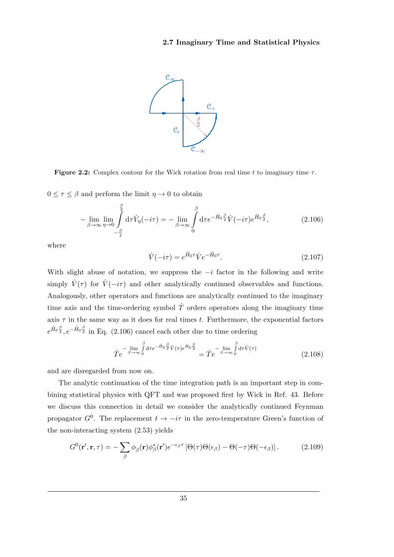
Figure 2.2: Complex contour for the Wick rotation from real time t to imaginary time τ .
0 ≤ τ ≤ β and perform the limit η → 0 to obtain
− limβ→∞
limη→0
β2∫
−β2
dτ Vη(−iτ) = − limβ→∞
β∫0
dτe−H0β2 V (−iτ)eH0
β2 , (2.106)
where
V (−iτ) = eH0τ V e−H0τ . (2.107)
With slight abuse of notation, we suppress the −i factor in the following and write
simply V (τ) for V (−iτ) and other analytically continued observables and functions.
Analogously, other operators and functions are analytically continued to the imaginary
time axis and the time-ordering symbol T orders operators along the imaginary time
axis τ in the same way as it does for real times t. Furthermore, the exponential factors
eH0β2 , e−H0
β2 in Eq. (2.106) cancel each other due to time ordering
T e− limβ→∞
β∫0
dτe−H0β2 V (τ)eH0
β2
= T e− limβ→∞
β∫0
dτV (τ)(2.108)
and are disregarded from now on.
The analytic continuation of the time integration path is an important step in com-
bining statistical physics with QFT and was proposed first by Wick in Ref. 43. Before
we discuss this connection in detail we consider the analytically continued Feynman
propagator G0. The replacement t → −iτ in the zero-temperature Green’s function of
the non-interacting system (2.53) yields
G0(r′, r, τ) = −∑β
φβ(r)φ∗β(r′)e−εβτ [Θ(τ)Θ(εβ)−Θ(−τ)Θ(−εβ)] . (2.109)
35

2. QUANTUM FIELD THEORY FOR CONDENSED MATTER
Thus, in contrast to real time, the Feynman propagator is a decaying and non-oscillating
function in imaginary time τ . This is a favorable property for practical calculations
allowing for accurate representations of G0 on coarse imaginary time grids. We exploit
this property in chapter 5 extensively.
2.7.1 Finite-Temperature Feynman Propagator
To bridge the gap to statistical physics we follow Ref. 44 and introduce the density
matrix of N non-interacting electrons
ρ0 =e−βH0
Z0(β), Z0(β) =
∞∑µ=0
〈Ψµ| e−βH0 |Ψµ〉 . (2.110)
with the zero-temperature limit β →∞ given by
limβ→∞
ρ0 = |Ψ0〉 〈Ψ0| . (2.111)
For further reference the notation 〈·〉β is introduced to indicate ensemble averages w.r.t.
the non-interacting system
⟨O(τ)
⟩β
=∞∑µ=0
〈Ψµ| ρ0O(τ) |Ψµ〉 = Trρ0O(τ)
(2.112)
for an operator O. Then (2.109) is the zero-temperature limit β → ∞ of the non-
interacting finite-temperature Green’s function
G0(r′, r, τ) = −⟨T ψ(r, τ)ψ†(r′, 0)
⟩β. (2.113)
We use the same symbol G0 for both, the zero and finite-temperature Green’s function,
because the former can always be recovered from the latter by taking the limit β →∞.
Considering the finite-temperature case has the advantage of exploiting the property,
see Ref. 30, 45,
G0(r′, r, τ + β) = −G0(r′, r, τ), (2.114)
36

2.7 Imaginary Time and Statistical Physics
which follows from the antiperiodicity of the trace1
⟨ψ(r, τ + β)ψ†(r′)
⟩β
=1
Z0(β)Tre−βH0e(β+τ)H0ψ(r)e−(β+τ)H0ψ†(r′)
=
1
Z0(β)TreτH0ψ(r)e−τH0e−βH0ψ†(r′)
=
1
Z0(β)Tre−βH0ψ†(r′)eτH0ψ(r)e−τH0
=⟨ψ†(r′)ψ(r, τ)
⟩β
= −⟨T ψ(r, τ)ψ†(r′)
⟩β, τ < 0.
(2.115)
It can be shown, see Ref. 45, that the orbital representation of the finite temperature
Green’s function is given by
G0(r′, r, τ) = −∑α
φα(r)φ∗α(r′)e−εατ [Θ(τ)(1− fβ(εα))−Θ(−τ)fβ(εα)] , (2.116)
where fβ is the Fermi occupancy function
fβ(ε) =1
eβε + 1. (2.117)
The convergence of the finite-temperature Green’s function G0 is guaranteed only for
the interval −β ≤ τ ≤ β. One, therefore, continues G0(τ) antiperiodically onto the
complete real line, so that the function can be decomposed into a Fourier series
G0(r′, r, τ) =1
β
∞∑n=−∞
e−iωnτG0(r′, r, iπn
β), (2.118)
with coefficients
G0(r′, r, iπn
β) =
1
2
∫ β
−βdτe
iπnβτG0(r′, r, τ), n ∈ Z (2.119)
In the zero-temperature limit β →∞, the Fourier spectrum becomes continuous iπnβ →iω and take arbitrary values on the imaginary frequency axis iω. Consequently, in
agreement with Fourier analysis, the series representation (2.118) becomes a Fourier
integral
G0(r′, r, τ) =1
2π
∞∫−∞
dωe−iωτG0(r′, r, iω), β →∞. (2.120)
1The same follows for τ > 0.
37

2. QUANTUM FIELD THEORY FOR CONDENSED MATTER
We emphasize that on the imaginary frequency axis the Green’s function is well-behaved,
due to
G0(r′, r, iω) =∑α
φα(r)φ∗α(r′)
iω − εα, (2.121)
and no branch cut is crossed when approaching ω → εα as in the case for real frequencies,
see section 2.4.1. Hence, the imaginary frequency integration in Eq. (2.120) can be
carried out straightforwardly and a deformation of the integration contour, as in (2.68),
is not necessary.
-1
-0.5
0
0.5
1
−β −β2 0 β
2 β
G0(τ
)
τ
Figure 2.3: Typical imaginary time-dependence of the non-interacting propagator G0 il-
lustrating the anti-periodicity property (2.114). Here a two-state model with one occupied
state with energy ε1 = −1.5 eV and an unoccupied state with energy ε2 = 2.3 eV for a
inverse temperature of β = 10 eV−1 is shown.
For finite temperatures, however, it is sufficient to restrict the imaginary time interval
either to 0 ≤ τ ≤ β or to −β2 ≤ τ ≤
β2 , as shown in Fig. 2.3. In this work we exclusively
use the former interval 0 ≤ τ ≤ β, where the representations (2.118) and (2.119) read
G0(r′, r, τ) =1
β
∞∑n=−∞
e−iωnτG0(r′, r, iωn) (2.122)
G0(r′, r, iωn) =
∫ β
0dτeiωnτG0(r′, r, τ), n ∈ Z (2.123)
38

2.7 Imaginary Time and Statistical Physics
and the discrete Fourier spectrum iωn is restricted to the fermionic Matsubara frequencies
ωn =(2n− 1)π
β, n ∈ Z. (2.124)
This follows from Eqs. (2.118) and (2.119) by shifting the integration variable on the
interval [−β, 0] in Eq. (2.119) to τ → τ + β and using property (2.114), see Ref. 45.
2.7.2 Statistical Physics and Imaginary Time
One introduces the interacting partition function Z(β) and the corresponding density
operator ρ of the system
Z(β) = Tre−βH
, ρ =
exp(−βH)
Z(β)(2.125)
where the trace is evaluated w.r.t. the interacting eigenstates |Ωµ〉. This partition
function can be used to compute the ensemble average TrρOH(τ)
of an arbitrary
Heisenberg-operator
OH(τ) = eβHOe−βH . (2.126)
With the help of the Gell-Mann and Low theorem and the property
e−βH = e−βH0 S(−iβ, 0)︸ ︷︷ ︸=S(β)
= Z0(β)ρ0S(β), (2.127)
see Refs. 45, 46,1 the trace w.r.t. interacting eigenstates |Ωµ〉 can be rewritten into
a trace w.r.t. to the non-interacting eigenstates∣∣∣Ψ(N)
µ
⟩. For instance, the partition
function Z(β) can be expressed as
Z(β) = Z0(β)Trρ0(β)S(β)
= Z0(β)
⟨S(β)
⟩β
(2.128)
to separate the grand partition function into
Z(β) = Z0(β)Zv(β) (2.129)
with the interacting part Zv(β) given by
Zv(β) =⟨S(β)
⟩β. (2.130)
1 Eq. (2.127) follows from analytic continuation of (2.77) using t→ −iβ.
39

2. QUANTUM FIELD THEORY FOR CONDENSED MATTER
Alternatively, the grand canonical potential Φ of the system can be written as
Φ = − 1
βlnZ(β) = − 1
β[lnZ0(β) + lnZv(β)] = Φ0 + Φv (2.131)
or the internal energy E of the system can be computed via
E = − ∂
∂βlnZ(β) = − ∂
∂β[lnZ0(β) + lnZv(β)] =
⟨H0
⟩β
+Z0(β)
Zv(β)
⟨S(β)V
⟩β. (2.132)
In particular, one obtains for the zero-temperature limit β →∞, a representation of the
interacting groundstate energy
Ω0 = limβ→∞
E = 〈Ψ0| H0 |Ψ0〉︸ ︷︷ ︸E0
+〈Ψ0| T e−
∫∞0 dτV (τ)V |Ψ0〉
〈Ψ0| T e−∫∞0 dτV (τ) |Ψ0〉
. (2.133)
It is interesting to compare this expression with the Gell-Mann and Low expression for
the interacting eigenenergies (2.101). It is not difficult to show, see [44, 46], that in
general thermal averages of Heisenberg-operators (2.126) can be expressed as
TrρOH(τ)
=
∞∑µ=0
〈Ωµ| ρOH(τ) |Ωµ〉 =
⟨S(β)T O(τ)
⟩β⟨
S(β)⟩β
. (2.134)
In general, all observables are expressible in terms of field and conjugate field opera-
tors ψ, ψ†.1 Therefore, it is convenient to introduce the generating functional of QFT,
following Refs. 39, 47,
W[j, j∗] = ln
⟨S(β)T e
−β∫0
dτ∫
dr(j†(r,τ)ψ(r,τ)+ψ(r,τ)j∗(r,τ))⟩β
(2.135)
from which arbitrary expectation values of the interacting system can be calculated
as functional derivatives w.r.t. source fields j, j∗. Specifically, the interacting finite-
temperature propagator G, discussed in detail in chapter 4.1.1, can be written as
G(r′, r, τ) =
∞∑µ=0
〈Ωµ| ρT ψH(r, τ)ψ†H(r′) |Ωµ〉 (2.136)
= − δ2W[j, j∗]
δj∗(r′)δj(r, τ)
∣∣∣∣j,j∗=0
(2.137)
= −
⟨S(β)T ψ(r, τ)ψ†(r′)
⟩β⟨
S(β)⟩β
. (2.138)
1Similarly in classical Hamiltonian mechanics, every observable is expressible in terms of conjugate
variables q, p.
40

2.7 Imaginary Time and Statistical Physics
All expressions so far are exact. However, in practice one has to evaluate the in-
teracting expectation values (2.134) perturbatively. For this purpose the diagrammatic
method is introduced in the following section.
41

2. QUANTUM FIELD THEORY FOR CONDENSED MATTER
42

3
Many-Body Perturbation Theory
3.1 Perturbation Series of the Grand Canonical Potential
Due to the complex structure of Eq. (2.128) it is hopeless to evaluate the grand canonical
potential Φ with Eq. (2.131) exactly. The same holds true for the zero-temperature case1
Ω0 = limβ→∞
Φ, (3.1)
so that one has to rely on approximations. Fortunately, the expressions for the parti-
tion function and canonical potential, presented in the previous section, provide a good
starting point.
For this purpose one expands the exponential in the interacting partition function
Zv(β), defined in Eq. (2.130), into a series
Zv(β) =⟨S(β)
⟩β
=
⟨T e−β∫0
dτV (τ)⟩β
(3.2)
allows for a perturbative treatment of the interacting degrees of freedom. In particular,
1This identity holds true, due to our convention µ = 0.
43
3. MANY-BODY PERTURBATION THEORY
the zeroth, first and second order terms read
Z(0)v = 〈1〉β = 1 (3.3)
Z(1)v = −
β∫0
dτ⟨T V (τ)
⟩β
(3.4)
Z(2)v =
1
2
β∫0
dτ1dτ2
⟨T V (τ1)V (τ2)
⟩β
(3.5)
and the n order term is
Z(n)v =
(−1)n
n!
β∫0
dτ1 · · · dτn⟨T V (τ1) · · · V (τn)
⟩β
(3.6)
Inserting this expansion into Eq. (2.131) one obtains an approximative formula for the
interacting part Φv of the grand canonical potential
Φv = − 1
βlnZv(β) = − 1
βln(
1 + Z(1)v + Z(2)
v · · ·). (3.7)
In summary, the perturbation series of the grand canonical potential reduces to the
evaluation of time-ordered matrix elements of products of Coulomb operators V . In the
following section, we discuss the evaluation of these expectation values in detail.
3.1.1 The Wick Theorem
The Coulomb operator can be written in terms of two-particle integrals
V αβγδ = q2
∫drdr′
φ∗α(r)φ∗β(r′)φγ(r′)φδ(r)
|r− r′| = 〈φα, φβ| V |φδ, φγ〉 , (3.8)
and the creation and annihilation operators
V (τ) =1
2V αβγδ c†α(τ)c†β(τ)cγ(τ)cδ(τ). (3.9)
This follows from the normal-ordered operator (2.70) and the transformation rules (2.30)
and (2.31). As in the last expression we adopt the Einstein summation convention in the
following. Within this convention, the first order term of the partition function (3.4) is
Z(1)v = −
β∫0
dτ⟨T V (τ)
⟩β
= −1
2V αβγδ
β∫0
dτ⟨T c†α(τ)c†β(τ)cγ(τ)cδ(τ)
⟩β. (3.10)
44

3.1 Perturbation Series of the Grand Canonical Potential
Suppressing the imaginary time dependence τi for the operators c†αi , · · · cδi for the time
being, the nth order term (3.6) of the partition function reads
Z(n)v (β) =
(−1)n
n!
V α1β1γ1δ1 · · ·V αnβnγnδn
2n
β∫0
dτ1 · · · dτn⟨T c†α1
· · · cδn⟩β. (3.11)
Let us consider the zero-temperature limit β → ∞ of this expression for a moment. In
this limit the ensemble operator ρ0 reduces to the groundstate projector (2.111) and⟨T c†α1
· · · cδn⟩∞
= 〈Ψ0| T c†α1· · · cδn |Ψ0〉 , 0 < τ1, · · · , τn <∞ (3.12)
holds. To evaluate the r.h.s. one needs the Wick theorem, which uses the contraction of
two operators. This contraction is defined as
O(τ1)O(τ2) = T O(τ1)O(τ2)− : O(τ1)O(τ2) :, (3.13)
where the normal ordering operator : · : was introduced in Eq. (2.28). Specifically, for
the contraction of an annihilation and creation operator one obtains when applied to
the groundstate
〈Ψ0| cα(τ1)c†β(τ2) |Ψ0〉 = 〈Ψ0| T cα(τ1)c†β(τ2)− : cα(τ1)c†β(τ2) : |Ψ0〉
= 〈Ψ0| T cα(τ1)c†β(τ2) |Ψ0〉︸ ︷︷ ︸=−G0
βα(τ1−τ2)
−0, (3.14)
since the normal ordered product vanishes when acting on the Fermi vacuum, see Eqs.
(2.36) and (2.37). Here the object on the r.h.s. of Eq. (3.14) is the well-known non-
interacting Feynman propagator G0 in the one-particle basis
G0βα(τ1 − τ2) =
∫d3rd3r′φα(r′)G0(r′, r, τ1 − τ2)φ∗β(r), (3.15)
where it is diagonal
G0αβ(τ) = −δαβe−εατ [Θ(τ)Θ(εα)−Θ(−τ)Θ(−εα)] ≡ δαβG0
α(τ). (3.16)
With this definitions the Wick theorem can be formulated in the following way, see
Refs. 34, 46.
45

3. MANY-BODY PERTURBATION THEORY
Theorem 3.1.1 (Wick Theorem) A time-ordered product of operators Oi = O(ti) in
the interaction picture, can be decomposed into a normal-ordered sum of all possible
contractions, i.e.
T (O1O2 · · · On) = : O1O2O3 · · · On : + : O1O2O3O4 · · · On :
+ : O1O2O3O4 · · · On : + · · · (3.17)
The proof of this statement can be found in every good book about QFT, for instance
Refs. 34, 46, and will not be given here.
The Wick theorem is a powerful utility when applied to the r.h.s. of Eq. (3.12). On
the one side, only contractions between creation and annihilation operators remain, due
to the orthogonality of the Slater determinants⟨Ψ(N)µ
∣∣∣ Ψ(M)ν
⟩= δNMδµν . (3.18)
On the other side, only fully contracted terms survive, because terms like
: c†αc†β cγ cδ := − : c†αcγ c
†β cδ := − c†αcγ : c†β cδ : (3.19)
vanish when evaluated for the groundstate
〈Ψ0| − c†αcγ : c†β cδ : |Ψ0〉 = 0. (3.20)
Evidently, all orders of the interacting energy Ω0 at zero-temperature in Eq. (3.1) are
expressible in terms of the non-interacting Green’s function G0α and the Coulomb matrix
elements Vαβγδ.
This conclusion relies on the Fermi vacuum properties (2.36) and (2.37), implying Eq.
(3.14), and is not valid a priori for finite-temperatures β <∞. This is due to the presence
of excited Slater determinants∣∣∣Ψ(N)
µ
⟩in the thermal averages 〈· · ·〉β. However, one can
show that all normal-ordered thermal averages⟨
: cαc†β :⟩β
vanish in the thermodynamic
limit, see Ref. 46, and consequently Eq. (3.14) is ultimately valid also for finite β.
Equipped with this knowledge, we evaluate the first two orders of the partition
function Zv(β) given in Eqs. (3.3)-(3.5) in the next section using the diagrammatic
method.
46

3.2 Feynman Diagrams
δ
α
β
γ
Figure 3.1: Labeled diagram for the interaction matrix element G0αG
0βV
αβγδG0γG
0δ .
3.2 Feynman Diagrams
We start with the first order term Z(1)v given in Eq. (3.4). Using the Wick theorem 3.17
and suppressing the τ -dependence in the notation, the corresponding interaction matrix
elements (3.10) can be written as⟨T c†αc
†β cγ cδ
⟩β
= −⟨T cγ c
†α
⟩β︸ ︷︷ ︸
−G0αγ(0)
⟨T cδ c
†β
⟩β︸ ︷︷ ︸
−G0βδ(0)
+⟨T cδ c
†α
⟩β︸ ︷︷ ︸
−G0αδ(0)
⟨T cβ c
†γ
⟩β︸ ︷︷ ︸
−G0βγ(0)
. (3.21)
Hence the first order term of the partition function reads
Z(1)v = −β
2
(G0α(0)G0
β(0)V αβαβ −G0α(0)G0
β(0)V αββα). (3.22)
Here, we note that the quantity G0α(0) is always evaluated as lim
τ0G0α(τ) and corresponds
to the density matrix.
It is convenient to visualize specific contractions, including those above, with the
help of diagrams, originally proposed by Feynman to evaluate matrix elements in QED,
see Ref. 48. This method is adopted as follows. Green’s functions G0α are represented
by directed linesα
and interaction matrix elements V αβγδ by wiggly lines .
Particle lines attach to interaction lines at vertices, represented by dots , as shown
in Fig. 3.1. Typically, the horizontal direction represents time, whereas the vertical
direction stands for spatial coordinates. However, as one shall see in a moment, only the
topology of the diagrams is important, so that in the end it does not matter weather the
diagrams are drawn vertically or horizontally.
Using these prescriptions the two terms in Eq. (3.22) can be visualized as shown in
Fig. 3.2 and are called Hartree and Fock diagrams. These names come from the facts
that, the two terms in Eq. (3.22) assume the of form of the Fock-exchange 〈φαφβ| |r −r′|−1 |φβφα〉 and the Hartree energy 〈φαφβ| |r− r′|−1 |φαφβ〉 [compare to section 1.1].
To gain more insight, one proceeds with the evaluation of higher order terms of the
partition function, however, this must be done carefully. The naive application of the
47

3. MANY-BODY PERTURBATION THEORY
β
α
α β
Figure 3.2: Hartree (right) and Fock diagram (left).
β αδ γ δ α γβ
Figure 3.3: Ladder (left) and bubble (right) contraction as labeled diagrams.
Wick theorem to each term of the perturbation series (3.11) is problematic, since the
number of non-zero contractions increases exponentially with order n. For instance in
second order, there are 24 non-trivial contributions, two of them are shown in Fig. 3.3.
For n = 3 one has 6 × 5 × 4 × 3 × 2 = 720 possible contributions and in general for
order n there are in total (2n)! labeled diagrams, see Ref. 32, 39. To deal with this large
number of different contractions we follow Negele and Orland and consider two different
symmetries.
On the one side, one can exploit the symmetry of the interaction matrix elements
V αβγδ = V βαδγ , (3.23)
which follows from the change of the spatial integration variable in Eq. (3.8). This prop-
erty implies that two labeled diagrams are equivalent, if the exchange of two incoming
and outgoing particle lines at one vertex yields topologically the same diagram. In total
there are 2n possible exchanges for a diagram with n interaction lines. On the other side,
one obtains the same contribution if two permutations σ, σ′ ∈ Sn of the time integration
variables τσ(1), · · · , τσ(n) and τσ′(1), · · · , τσ′(n) yield the same diagram. For n interactions
this yields n! possible permutations. In the following, these symmetries are considered
from a more general point of view to deduce a simple summation rule for diagrams.
A general transformation θ from one diagram γ to another diagram θγ = γ′ is a
combination of (3.23) and permutations in τ1 · · · τn. The set of all possible transforma-
tions θ yields a group Γ and has 2nn! elements in total. We call two transformations
θ, θ′ ∈ Γ equivalent θ ' θ′, if they transform topologically into the same graph, that is
48

3.2 Feynman Diagrams
Figure 3.4: Disconnected unlabeled diagrams in second order. The symmetry factors (from
left to right) are 8, 4 and 8.
Figure 3.5: Second order irreducible, connected diagrams. With symmetry factors
4, 4, 2, 2, 1 (from left to right).
θγ, θ′γ and γ yield the same contribution to the partition function Z(β). This defines
equivalence classes Hγ , and Sγ denotes the number of elements in Hγ ,i.e. the number of
topologically equivalent diagrams contained in Hγ . Because Hγ is a subgroup of Γ, Sγ
must be a divisor of 2nn! and 2nn!/Sγ ∈ N. Then the diagram γ appears 2nn!/Sγ times
for order n, resulting in an effective 1/Sγ symmetry factor in the partition function Z(β)
for the equivalence class of γ. The diagram γ defining the equivalence class Hγ is called
irreducible and is represented by an unlabeled diagram, where the indices α, β · · · of the
wiggly and particle lines are suppressed.
In practice, one, therefore, translates only the irreducible diagrams for a given order
into integrals and multiplies the result by the corresponding symmetry factor 1/Sγ . As
an consistency check, one may use the following sum rule, valid for each order∑γ
1
Sγ=
(2n)!
n!2n= (2n− 1)(2n− 3)(2n− 5) · · · = (2n− 1)!!, (3.24)
where the sum on the r.h.s. is over all irreducible (topologically equivalent) diagrams
for order n.
As an example we show in Figs. 3.5 and 3.4 all irreducible graphs for the second
order with the corresponding symmetry factors. For instance the symmetry property
of Eq. (3.23) yields 2 × 2 = 4 identical contributions for the first diagram in Fig. 3.4
and for each contribution there are only 2 possible rearrangements of the integration
variables τ1, τ2 yielding topologically the same diagram, so that in total a symmetry
49

3. MANY-BODY PERTURBATION THEORY
A B C DFigure 3.6: Illustration of the symmetry factor of diagram A. Diagram B is obtained from
A using Eq. (3.23) for the upper interaction line, whereas diagram C follows from B using
the same identity for the lower one and diagram D is obtained from C after exchanging
τ1 ↔ τ2. Only diagram A and D belong to the same equivalence class with symmetry factor
Sγ = 2, because they are topologically the same directed graph.
factor of Sγ = 23 = 8 is obtained. The forth diagram in Fig. 3.5 has a symmetry
factor of Sγ = 2, because there is only one symmetry operation giving the same result:
The exchange of both horizontal vertices (using Eq. (3.23)) combined with a change
of the integration variables τ1 ↔ τ2. This symmetry operation is illustrated in Fig.
3.6. Analogously, the symmetry factors of other diagrams are obtained, see Ref. 39
for a comprehensive discussion. In summary, the 24 labeled diagrams for n = 2 can be
grouped into 8 equivalence classes Hγ and the sum over all inverse symmetry factors
1/Sγ , see caption of Figs. 3.5 and 3.4, yields 3 and satisfies Eq. (3.24).
One can reduce the relevant number of diagrams even further using the so-called
linked cluster theorem. This theorem was published by Goldstone in Ref. 49 and proved
for the groundstate energy at zero temperature. However, it can be shown that a similar
theorem holds for finite temperatures, see Ref. 46. Here we present the linked cluster
theorem as formulated by Abrikosov et al.
Theorem 3.2.1 (Linked Cluster Theorem) The perturbation series of lnZβ con-
tains only connected diagrams.
Diagrams as in Fig. 3.4, which separate into smaller order subdiagrams, are called
disconnected, whereas those in Fig. 3.5, are named connected. Hence, only connected,
topologically distinct contractions need to be determined for the perturbative analysis
of the grand canonical potential Φ.
We summarize the results of this section by formulating following Feynman rules
for the diagrammatic expansion of the grand canonical potential. Similar rules for the
Fourier domain can be found elsewhere, see for instance Refs. 34, 39, 46, and are not
discussed here.
50

3.2 Feynman Diagrams
Feynman rules in one-particle basis
f1 Draw all connected, topologically distinct diagrams for each order n.
f2 Assign an imaginary time τ and an one-particle index α to each particle line and
include the factor G0α(τ).
f3 For each interaction line include the factor V αβγδ.
f4 Multiply the result by the factor (−1)n(−1)l
Sγ, where l is the number of closed particle
loops and Sγ the symmetry factor of the graph.1
f5 Integrate over imaginary times in [0, β] and sum over all one-particle indices.
In analogy to the one-particle basis, similar Feynman rules can be formulated in position
space and imaginary time.
Feynman rules for spacetime domain
F1 Draw all connected, topologically distinct diagrams for each order n.
F2 Assign a spacetime point x = (r, τ) to each vertex.
F3 For each wiggly line starting at x′ = (r′, τ ′) and ending in x = (r, τ) assign a
factor δ(τ−τ ′)|r−r′| . Analogously, assign a factor G0(r′, r, τ − τ ′) to each particle line
originating in x′ and ending in x.
F4 Multiply the result by the factor (−1)n(−1)l
Sγ, where l is the number of closed particle
loops and Sγ the symmetry factor of the graph.
F5 Integrate over spacetime points x in the domain [0, β] × C, where C is the unit
cell.
Both sets of rules hold for the zero-temperature case as well, with the difference that
finite-temperature propagators are replaced by their zero-temperature limit and integra-
tion is performed over [0,∞).
Nevertheless, the number of distinct, irreducible and connected diagrams becomes
huge and intractable with increasing order. Even worse, often diagrams, such as the
1The reason for the loop contribution can be found in Ref. 39.
51

3. MANY-BODY PERTURBATION THEORY
+ ++ + + · · ·
Figure 3.7: Random Phase Approximation for the grand canonical potential.
bubble graphs in Fig. 3.3 diverge for each order in perturbation theory for prototypical
systems such as the HEG, see Ref. 33. However, Gell-Mann and Brueckner showed that
evaluating the infinite sum of all bubble diagrams yields a finite result, see Ref. 12.
This technique, that is summation over all orders of specific equivalence classes, is the
true power of the diagrammatic method. In the following the rules F1-F5 are applied to
the subset of all bubble graphs and an approximation for the interacting grand canonical
potential is obtained.
3.3 Random Phase Approximation
Restricting the perturbation series of the grand-canonical potential to the subset of all
bubble diagrams, see Fig. 3.7, one obtains the so-called random phase approximation
(RPA). The RPA is widely used in condensed matter physics today, due to two reasons.
First, the RPA yields accurate estimates for the grand canonical potential Φ, respectively
the interacting groundstate energy Ω0, and becomes exact for the HEG in the asymptotic
limit rs ≈ 0 yielding an energy density given by Eq. (1.37). Second, the RPA can be
calculated with a decent computational effort. The latter is due to its simple expression,
which is derived in the following with the methods learned from the previous section.
As a first step, one observes, that the symmetry factor Sγ for each diagram beyond the
first order is twice the number of cyclic permutations of τσ(1) · · · τσ(n), so simply 2n.[39]
Second, it is useful to work with the independent-particle polarizability χ0, defined by
χ0(r′, r, τ − τ ′) = (−1)× x′x
= −G0(r′, r, τ − τ ′)G0(r, r′, τ ′− τ). (3.25)
With this definition and the Feynman rules F1-F5 from previous section, the second
52

3.3 Random Phase Approximation
and third order diagram can be written as
Φ(2) = − 1
β
(−1)2(−1)2
4
β∫0
dτ1dτ2Tr
[χ0(r2, r1, τ2 − τ1)χ0(r4, r3, τ1 − τ2)
|r1 − r4||r2 − r3|
](3.26)
Φ(3) = − 1
β
(−1)3(−1)3
6
β∫0
dτ1dτ2dτ3
× Tr
[χ0(r2, r1, τ2 − τ1)χ0(r4, r3, τ4 − τ2)χ0(r5, r6, τ4 − τ1)
|r1 − r6||r2 − r3||r4 − r5|
]. (3.27)
Here Tr indicates spatial integration over all coordinates r1, r2, · · · . Higher order terms
contain higher order convolutions in imaginary time.
These expressions can be further simplified by exploiting the periodic property
χ0(r′, r, τ + β) = χ0(r′, r, τ), (3.28)
which follows from the antiperiodicity of the non-interacting propagator (2.114) and is
illustrated in Fig. 3.8 using the same model for G0 as in Fig. 2.3. This allows to
decompose the independent-particle polarizability χ0 into a Fourier series
χ0(r′, r, τ) =1
β
∞∑m=−∞
e−iνmτχ0(r′, r, iνm) (3.29)
with coefficients
χ0(r′, r, iνm) =
∫ β
0dτeiνmτχ0(r′, r, τ), m ∈ Z. (3.30)
Here, the bosonic Matsubara frequencies
νn =2mπ
β, m ∈ Z (3.31)
are used in Eqs. (3.29) and (3.30) rather than their fermionic counterparts ωn. Inserting
Eq. (3.29) into Eq. (3.26) and using the completeness relation∫dτe−iτ(νm−νm′ ) = βδmm′ , (3.32)
the imaginary-time integrals in Eq. (3.26) reduce to a simple Matsubara sum
Φ(2) = − 1
4β
∞∑n=−∞
Tr
[χ0(r2, r1, iνn)χ0(r4, r3, iνn)
|r1 − r4||r2 − r3|
]︸ ︷︷ ︸
Tr[χ0(iνn)V ]2
. (3.33)
53

3. MANY-BODY PERTURBATION THEORY
-1
-0.5
0
0.5
1
−β −β2 0 β
2 β
χ0(τ
)
τ
Figure 3.8: Typical imaginary time-dependence of the independent-particle polarizability
χ0 illustrating the periodic property (3.28). Here a two-state model with one occupied state
with energy ε1 = −1.5 eV and an unoccupied state with energy ε2 = 2.3 eV for a inverse
temperature of β = 10 eV−1 is shown.
The same holds true for arbitrary order
Φ(n) = −(−1)2n
2β
∞∑m=−∞
Tr[χ0(iνm)V
]nn
. (3.34)
Finally, using the power series of the logarithm
ln(1− x) = −∞∑n=1
xn
n, (3.35)
one obtains for the sum of all bubble diagrams
ΦRPAc =
1
2β
∞∑m=−∞
Tr
ln[1− χ0(iνm)V
]+ χ0(iνm)V
. (3.36)
Specifically, for the zero-temperature limit β → ∞, this yields ERPAc , the correlation
energy of the RPA
ERPAc =
1
4π
∞∫−∞
dνTr
ln[1− χ0(iν)V
]+ χ0(iν)V
, (3.37)
54
3.3 Random Phase Approximation
with the zero-temperature polarizability on the imaginary frequency axis having the
form
limβ→∞
χ0(r′, r, iν) =∑ia
φi (r′)φ∗i (r)φa(r)φ∗a(r
′)2ξai
ξ2ai + ν2
, ξai = εa − εi > 0. (3.38)
Here i indicates an occupied and a an unoccupied one-particle index, see section 1.2.
The last expression follows straightforwardly from the general contraction formula (3.25),
the orbital representation of the Feynman propagator (2.109) and an additional Fourier
transformation to Matsubara space. Expression (3.37) follows also from the so-called
adiabatic connection fluctuation dissipation theorem (ACFDT), so that Eq. (3.37) is
sometimes called the ACFDT formula. The reader is referred to Ref. 50 for more
details.
In practical calculations, one determines the Fourier representation χ0q(g,g′, iν) of
Eq. 3.38 and calculates the RPA correlation energy as
ERPAc =
1
4π
n∑k=1
γk1
Nq
∑gg′q
[ln(1− χ0V
)]q
(g,g′, iνk) + χ0q(g,g′, iνk)Vq(g,g′)
,
(3.39)
where g,g′ represent reciprocal lattice vectors, q a point in the first Brillouin zone,
γk, νknk=1 a frequency integral quadrature and
Vq(g,g′) =δgg′
|q + g|2(3.40)
the Coulomb potential in reciprocal space. It is common to calculate the Fourier repre-
sentation χ0q(g,g′, iνk) directly from the Adler and Wiser formula[51, 52]
χ0qg,g′, iν) =
1
Nk
∑nn′k
2ξaiξ2ai + ν2
〈φi| ei(g+q)r |φa〉 〈φa| e−i(g′+q)r′ |φi〉 , (3.41)
with i = (n,k) denoting the occupied and a = (n′,k + q) the unoccupied Bloch index.
This approach is widely used in the community, although the unfavorable scaling of Eq.
3.41 (roughly with O(N4)) bears an obstacle to compute RPA energies for large systems.
In principle, one is able to evaluate χ0 with O(N3) scaling using the imaginary
time Green’s functions G0(r, r′, τ) and equation (3.25). This approach was discussed by
Rojas et al.[53] and was recently implemented for molecules by Foerster et al.[54] and
by Moussa[55], but a cubic-scaling RPA algorithm for periodic systems has not been
implemented. In chapter 5 we develop an efficient zero-temperature RPA algorithm,
55

3. MANY-BODY PERTURBATION THEORY
based on the considerations from this section and apply the method to calculate Si-
defect energies for large unit cells.
So far only the grand potential, respectively total energies have been considered.
In the following chapter we discuss how to determine spectral properties of many-body
systems using a set of coupled equations.
56

4
Spectral Properties
In chapter 3 a diagrammatic perturbation series for the interacting grand canonical
potential was derived, respectively the correlation energy at zero-temperature. This
chapter is dedicated to spectral properties, which can be described by the interacting
propagator G as the solution of the Schwinger-Dyson equations. To solve these equations
approximately, in the following two complementary approaches are considered, known
as the GW [see section 4.2.1] and the dynamical mean field approximation [see section
4.5.1].
4.1 Schwinger-Dyson Equations
In this section the diagramatic technique is extended in order to find a set of self-
consistent equations, that describes the spectral properties of the system in terms of
three quantities, the propagator G, the effective interaction W and the vertex function
Γ. The resulting three equations are known as Schwinger-Dyson equations and are
discussed in sections 4.1.1, 4.1.2 and 4.1.3 separately. Fairly heuristic arguments are
used to derive these equations, since the only purpose of this section is to give the basic
idea of this approach. The reader is referred to the literature for a mathematically
rigorous derivation.[44, 56, 57]
4.1.1 Interacting Green’s Function and Self-energy
We start with the interacting Feynman propagator G. This function describes the propa-
gation of an interacting electron (respectively hole) from one spacetime point to another
57

4. SPECTRAL PROPERTIES
and was already defined in Eq. (2.138). In analogy to the partition function Z(β), see
section 3.1, the expansion of the S-matrix into a power series yields a perturbation series
for the interacting propagator
G(r′, r, τ) = −∞∑n=0
(−1)n
n!
β∫0
dτ1 · · · dτn
⟨T V (τ1) · · · V (τn)ψ(r, τ)ψ†(r′)
⟩β
Z(n)v (β)
, (4.1)
where Z(n)v (β) is the interacting partition function given in Eq. (3.6). The matrix
elements in the denominator and numerator can be evaluated using Wick’s theorem
(3.17) and the resulting contractions can be visualized with Feynman diagrams. Here,
in contrast to the grand canonical potential, each diagram differs topologically, so that
the symmetry factor of each diagram is 1, see Ref. 39 for more details.
However, it can be shown that the denominator in Eq. (4.1) cancels all disconnected
diagrams of the numerator.1 Consequently, as in the case of the grand canonical potential
Φ, the perturbation series (4.1) contains only connected diagrams. We, therefore, neglect
the denominator in the series above and rewrite the expression into
G(r′, r, τ) = −∞∑n=0
(−1)n
n!
β∫0
dτ1 · · · dτn⟨T V (τ1) · · · V (τn)ψ(r, τ)ψ†(r′)
⟩c
β, (4.2)
where the superscript c indicates, that only topologically connected diagrams are taken
into account.
The zero order term of Eq. (4.2) reduces to the non-interacting Green’s function G0,
defined in Eq. (2.113), whereas higher order terms can be evaluated with the Feynman
rules F1-F5 or f1-f5 of section 3.2. For instance the first order terms translate to integrals
as follows
x′ x = −∫
dx1dx2G0(x′, x1)G0(x1, x)
δ(τ1 − τ2)
|r1 − r2|G0(x2, x2) (4.3)
x′ x = −∫
dx1dx2G0(x′, x1)G0(x1, x2)
δ(τ1 − τ2)
|r1 − r2|G0(x2, x), (4.4)
1This follows from the Linked Cluster Theorem 3.2.1 and the fact that the propagator G can be
written as the derivative of lnZ, see Ref. 39.
58

4.1 Schwinger-Dyson Equations
where we have introduced the abbreviation∫
dx =∫
d3r∫ β
0 dτ for convenience. Anal-
ogously, higher order, for instance the second order terms shown in Fig. 4.1, can be
translated to integrals. Looking at this figure (or Eqs. (4.3), (4.4)), one clearly sees that
Figure 4.1: Second order contributions to the interacting Feynman propagator.
all diagrams have an incoming and an outgoing non-interacting Green’s function ’leg’.
The infinite number of terms between the incoming and outgoing Green’s function de-
fines the self-energy Σ, so that the interacting Green’s function satisfies the equation[34]
G(x′, x) = G0(x′, x) +
∫dx1
∫dx2G
0(x′, x1)Σ(x1, x2)G0(x2, x), x = (r, τ) (4.5)
The two-point quantity
Σ = + + + + + · · ·(4.6)
contains repeated insets of diagrams (third and forth diagram) and is therefore called
the reducible self-energy. These terms separate into irreducible self-energy diagrams,
if by cutting and removing a particle line, two disconnected self-energy diagrams are
obtained. For instance the third diagram in Eq. (4.6) contains two diagrams of the
first term, whereas the forth term contains the first and second diagram connected by a
propagator G0.
One takes advantage of this fact and defines the irreducible self-energy Σ, containing
only irreducible diagrams. With this, we obtain the first Schwinger-Dyson equation[33,
58]
G(x′, x) = G0(x′, x) +
∫dx1
∫dx2G
0(x′, x1)Σ(x1, x2)G(x2, x), (4.7)
which reads diagrammatically
= +Σ
(4.8)
59

4. SPECTRAL PROPERTIES
where the irreducible self-energy Σ is given by
Σ = + + + + · · ·(4.9)
and we used thick particle lines in Eq. (4.8) to indicate interacting Green’s functions G.
We emphasize that Σ and Σ obey a Dyson equation of the type
Σ(x′, x) = Σ(x′, x) +
∫dx1
∫dx2Σ(x′, x1)G0(x1, x2)Σ(x2, x), (4.10)
which follows trivially from comparison of Eqs. (4.5) and (4.7).[34]
The first term in the irreducible self-energy (4.9)
Σ(1)(x′, x) = −δ(x− x′)∫
dx3δ(τ3 − τ ′)|r3 − r′| G
0(x3, x3) (4.11)
is the time-independent Hartree term and is often absorbed in the non-interacting
Green’s function yielding the Hartree-dressed Green’s function G(1), indicated by a dou-
ble line in the following. The latter is obtained from the truncation of (4.9) after the
first term and solving the corresponding Dyson equation[33]
= + (4.12)
The Dyson equation for the full Green’s function, then reads
G(x′, x) = G(1)(x′, x) +
∫dx1dx2G
(1)(x′, x1)Σ(>1)(x1, x2)G(x2, x) (4.13)
respectively
= +Σ(>1)
(4.14)
with Σ(>1) being the exchange-correlation part Σ−Σ(1) of the irreducible self-energy[56]
Σ(>1) = + + + · · ·(4.15)
We note, that the exchange-correlation part Σ(>1) is expressed in terms of the Hartree
Green’s function G(1) rather than the non-interacting propagator G0. This procedure
above is, however, not restricted necessarily to the Hartree term. Instead, one can include
60

4.1 Schwinger-Dyson Equations
more terms in the irreducible self-energy and solve the corresponding Dyson equation
for the interacting Green’s function.
The general procedure is called renormalization and describes the inclusion of ir-
reducible (for instance the first n) self-energy terms in the skeleton (’non-interacting’
Green’s function G0). The resulting Green’s function G(n) is called dressed propagator
and describes physically the propagation of a renormalized quasi-electron (or quasi-hole).
These quasi-particles can be seen as bare electrons (holes) surrounded by a cloud of par-
ticles with heavier effective mass than their undressed counterparts. Due to the latter,
it can be expected that quasi-particles interact via an effective interaction W . This
interaction, also named screened interaction, is usually weaker than the bare interaction
V , so that one can expect that a perturbation series for the self-energy in terms of W
converges faster than Eq. (4.15).[33] As we shall see in a moment, the effective interac-
tion can be obtained by a similar renormalization procedure for the Coulomb interaction
V .
4.1.2 Effective Interaction and Polarizability
The instantaneous Coulomb interaction
V (x, x′) =δ(τ − τ ′)|r− r′| , x = (r, τ) (4.16)
can be seen as the (0, 0) component of the undressed electromagnetic Feynman-propagator
D0µν(x, x′) = −
⟨T Aµ(x)Aν(x′)
⟩β
(4.17)
in the Coulomb gauge, where Aµ is the field operator of the electromagnetic field. For
more information we refer the reader to Refs. 59, 60. Dyson showed (see Ref. 58), that
the corresponding interacting propagator Dµν satisfies an equation of the same kind as
the Dyson equation for the Green’s function (4.7). However, we are mostly interested
in the the (0, 0) components of this equation and write W (x, x′) = D00(x, x′) for the
dressed and V (x, x′) = δ(τ−τ ′)|r−r′| = D0
00(x, x′) for the bare propagator. Furthermore, we
do not assume that any spatial components of the bare and dressed photon-propagator
mix with the time components, so that W is a functional of V and G only.
61

4. SPECTRAL PROPERTIES
With these assumptions and the considerations from the previous section Eq. (4.5),
the following ansatz is obvious
W (x′, x) = V (x′, x) +
∫dx1
∫dx2V (x′, x1)χ(x1, x2)V (x2, x) (4.18)
Here χ is called the reducible polarizability and was introduced by Hubbard in Ref. 32. It
describes all possible polarization effects between two interaction lines, like for instance
the bubble polarization appearing in the second term of the self-energy
(4.15). An explicit expression of χ in terms of the density operator is given in section
4.2, here we indicate only the diagrammatic expansion
χ = + + + · · · .(4.19)
Comparing to (4.6), one sees that χ plays the same role for the screened interaction W
as the self-energy Σ for the Green’s function G. Thus, the validity of the analogue of
Eq. (4.10) can be assumed for the reducible polarizability
χ(x′, x) = χ(x′, x) +
∫dx1
∫dx2χ(x′, x1)V (x1, x2)χ(x′, x), (4.20)
in terms of the irreducible polarizability χ. In analogy to the irreducible self-energy, the
irreducible polarizability χ is defined by those subsets of the polarizability χ, that can
not be separated into more polarizability diagrams by cutting and removing a Coulomb
line V . For instance, the first and third diagram in Eq. (4.19) are irreducible, whereas
the second diagram is reducible.[33, 34]
Diagrams representing the expansion of χ were given first by Hedin in Ref. 56 and
are shown below
χ = + + + + + · · · .(4.21)
In analogy to the first Schwinger-Dyson equation (4.7), the second Schwinger-Dyson
equation for the screened interaction reads[56]
W (x′, x) = V (x′, x) +
∫dx1
∫dx2V (x′, x1)χ(x1, x2)W (x2, x). (4.22)
If indicates W in diagrams, the last expression translates to
= + χ. (4.23)
62

4.1 Schwinger-Dyson Equations
The introduction of the irreducible polarizability χ has two main advantages. First, χ
contains lesser terms than the reducible polarizability χ. Second, and more important,
it allows for a partial renormalization of the bare interaction V , i.e. an approximative
determination of the screened interaction W .[56]
One important approximation is obtained by truncating the series (4.21) after the
first term, that is approximating the independent particle polarizability by[34]
χ(x′, x) ≈ χ(1)(x′, x) = −G(n)(x′, x)G(n)(x, x′). (4.24)
Here the superscript n stands either for non-interacting, Hartree Green’s function G(1)
or any other dressed propagator. The RPA-type approximation (4.24) gives rise to the
screened interaction in the RPA
W (1)(x′, x) = V (x′, x) +
∫dx1
∫dx2V (x′, x1)χ(1)(x1, x2)W (1)(x2, x) (4.25)
translating to diagrams as
= +. (4.26)
The advantage of using dressed propagators G(n), respectively screened interactions W (n)
instead of skeleton propagators G0 and bare interactions V becomes evident already for
the first order approximations of Eq. (4.15) and Eq. (4.19). For instance, inserting the
RPA interaction W (1) of Eq. (4.26) for the bare interaction line in the first term of the
self-energy (4.15) generates a whole class of skeleton diagrams
= + + + · · ·. (4.27)
Higher order terms of the self-energy are then given by
Σ(>1) = + + + · · ·, (4.28)
where we indicated only one of six different third order terms, see Ref. 56.
Similarly, more terms in the irreducible polarizability can be taken into account
giving rise to other, more accurate, partially screened interactions W (n). Specifically for
W (1), the RPA interaction of (4.26), the screening Eq. (4.22) reads
W (x′, x) = W (1)(x′, x) +
∫dx1
∫dx2W
(1)(x′, x1)χ(>1)(x1, x2)W (x2, x). (4.29)
63
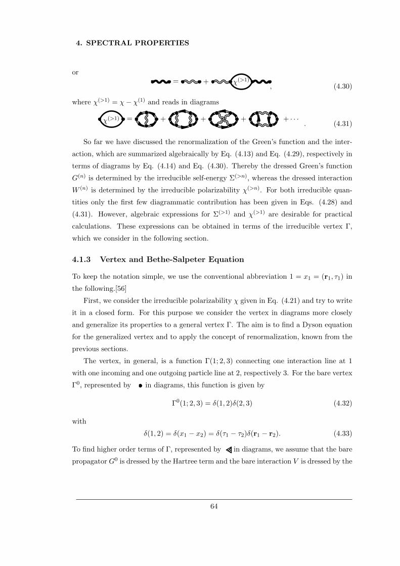
4. SPECTRAL PROPERTIES
or= + χ(>1)
, (4.30)
where χ(>1) = χ− χ(1) and reads in diagrams
χ(>1) = + + + + · · ·. (4.31)
So far we have discussed the renormalization of the Green’s function and the inter-
action, which are summarized algebraically by Eq. (4.13) and Eq. (4.29), respectively in
terms of diagrams by Eq. (4.14) and Eq. (4.30). Thereby the dressed Green’s function
G(n) is determined by the irreducible self-energy Σ(>n), whereas the dressed interaction
W (n) is determined by the irreducible polarizability χ(>n). For both irreducible quan-
tities only the first few diagrammatic contribution has been given in Eqs. (4.28) and
(4.31). However, algebraic expressions for Σ(>1) and χ(>1) are desirable for practical
calculations. These expressions can be obtained in terms of the irreducible vertex Γ,
which we consider in the following section.
4.1.3 Vertex and Bethe-Salpeter Equation
To keep the notation simple, we use the conventional abbreviation 1 = x1 = (r1, τ1) in
the following.[56]
First, we consider the irreducible polarizability χ given in Eq. (4.21) and try to write
it in a closed form. For this purpose we consider the vertex in diagrams more closely
and generalize its properties to a general vertex Γ. The aim is to find a Dyson equation
for the generalized vertex and to apply the concept of renormalization, known from the
previous sections.
The vertex, in general, is a function Γ(1; 2, 3) connecting one interaction line at 1
with one incoming and one outgoing particle line at 2, respectively 3. For the bare vertex
Γ0, represented by in diagrams, this function is given by
Γ0(1; 2, 3) = δ(1, 2)δ(2, 3) (4.32)
with
δ(1, 2) = δ(x1 − x2) = δ(τ1 − τ2)δ(r1 − r2). (4.33)
To find higher order terms of Γ, represented by in diagrams, we assume that the bare
propagator G0 is dressed by the Hartree term and the bare interaction V is dressed by the
64

4.1 Schwinger-Dyson Equations
RPA polarizability χ(1) and choose the following ansatz for the irreducible polarizability
χ =. (4.34)
This relation reads explicitly in terms of integrals
χ(1, 2) = −∫
d(1′)d(2′)Γ(1; 1′, 2′)G(1)(2, 1′)G(1)(2′, 2). (4.35)
The idea is to compare the r.h.s. of Eq. (4.34) with the diagrammatic expansion of χ
from Eq. (4.21), respectively Eq. (4.31), to determine the vertex function Γ. This is
straight forward for the first terms and we identify them as
= + + + + + · · ·
(4.36)
Next, we focus on the diagrammatic expansion of the irreducible self-energy Σ. Look-
ing at the diagrammatic expansion (4.28) it seems that the first three terms can be
summarized in following diagram
Σ(>1) =(4.37)
This relationship can be written explicitly as
Σ(>1)(1, 2) =
∫d(1′)d(2′)G(1)(1′, 2)W (1)(2′, 2)Γ(2′; 1, 1′) (4.38)
and was proven by Hedin in the 1960s.[56]
With Eqs. (4.38) and Eqs. (4.35) the irreducible self-energy and polarizability in the
Schwinger-Dyson equations for the Green’s function (4.7) respectively for the screened
interaction (4.22) can be eliminated, leaving only three unknown quantities G, W and
Γ. What remains is to find the equation for the irreducible vertex function.
For this reason one takes a close look at the diagrammatic series Eq. (4.36) and
’open’ the left vertex in each graph on the r.h.s. introducing the four-point irreducible
vertex Γ(1, 2; 3, 4) function. This quantity is indicated by
Γ(1, 2; 3, 4) =2
1
4
3
(4.39)
65

4. SPECTRAL PROPERTIES
in diagrams in the following and satisfies
Γ(1, 1; 3, 4) = Γ(1; 3, 4) =1
4
3
(4.40)
so that 2, 3 are incoming and 1, 4 are outgoing legs in Eq. (4.39). Similarly indicates
the bare four-vertex function
Γ0(1, 2; 3, 4) = δ(1, 3)δ(2, 4), (4.41)
as a generalization of the three-point quantity of Eq. (4.32).
Then the diagrammatic series (4.36) can be redrawn in a closed Schwinger-Dyson
form[44]
= + I(4.42)
translating to integrals as
Γ(1, 2; 3, 4) = Γ0(1, 2; 3, 4) +
∫d(1′) · · · d(6′)
× Γ0(1, 2; 3′, 4′)I(3′, 4′; 5′, 6′)G(1)(1′, 5′)G(1)(6′, 2′)Γ(1′, 2′; 3, 4).(4.43)
This equation is also known as the Bethe-Salpeter equation,[56, 61] where IGG is the
kernel of the equation. This kernel is the analogue of the Σ and χ for the Dyson equations
of the Green’s function (4.7) and the effective potential (4.22). The four-point object I is
called irreducible scattering amplitude and describes all necessary interactions between
particles and holes.[34, 44] To avoid double counting of diagrammatic contributions,
the amplitude contains only terms, irreducible in the particle-hole channel. That is,
diagrams of I do not separate into smaller order diagrams when ’cutting’ vertically
through a particle and a hole line. For instance the following scattering diagrams are
irreducible
and the following are reducible in the particle hole channel
66

4.1 Schwinger-Dyson Equations
An explicit expression for the scattering amplitude can be obtained from
I(n)(1, 2; 3, 4) =δΣ(n)(1, 2)
δG(n−1)(4, 3)(4.44)
for each order in perturbation theory.[62]
The three Schwinger-Dyson equations (4.43), (4.7) and (4.22) provide an alternative
view on a system of interacting electrons and allow for higher order approximations
beyond the HF or DFT method.[24, 34, 63] Here the approximation degree is determined
by the number of diagrams considered in the scattering amplitude I. For a comprehensive
overview of different approximations the reader is referred to Ref. 57.
67

4. SPECTRAL PROPERTIES
4.2 Hedin Equations and Self-Consistency Limit
The three Schwinger-Dyson equations (4.43), (4.7), (4.22) and the equations for the self-
energy (4.38) and polarizability (4.35) are known as Hedin equations among condensed
matter physicists.[56, 62, 64] The reason for this is mainly due to practical calculations,
where one has to solve the set of equations for Γ, χ, W , Σ and G self-consistently by
means of the scheme depicted in Fig. 4.2. This figure illustrates the iterative algorithm
to solve the Hedin equations
Σ(n) = G(n−1)W (n−1)Γ(n−1) (4.45)
G(n) = G(n−1) +G(n−1)Σ(n)G(n) (4.46)
I(n) =δΣ(n)
δG(n−1)(4.47)
Γ(n) = Γ(n−1) + Γ(n−1)I(n)G(n)G(n)Γ(n) (4.48)
χ(n) = −G(n)G(n)Γ(n) (4.49)
W (n) = W (n−1) +W (n−1)χ(n)W (n) (4.50)
with W (0) = V using following prescription[62]
Hedin Algorithm
H1 Calculate the self-energy Σ(n) with Eq. (4.45).
H2 Solve Eq. (4.46) for the dressed propagator G(n).
H3 Determine scattering amplitude from Eq. (4.47) (skip this step for n = 1).
H4 Solve Eq. (4.48) for the dressed vertex Γ(n).
H5 Compute the polarizability χ(n) with Eq. (4.49).
H6 Solve Eq. (4.50) for the dressed interaction W (n).
H7 Iterate H1-H6 until convergence is found.
Each iteration n of H1-H6 dresses the propagator G(n), interaction W (n) and vertex
function Γ(n) with more and more irreducible diagrams, so that in the self-consistency
limit n→∞ the iterative procedure converges to
G(n) → G, W (n) →W, Γ(n) → Γ, χ(n) → χ, Σ(n) → Σ, n→∞. (4.51)
68
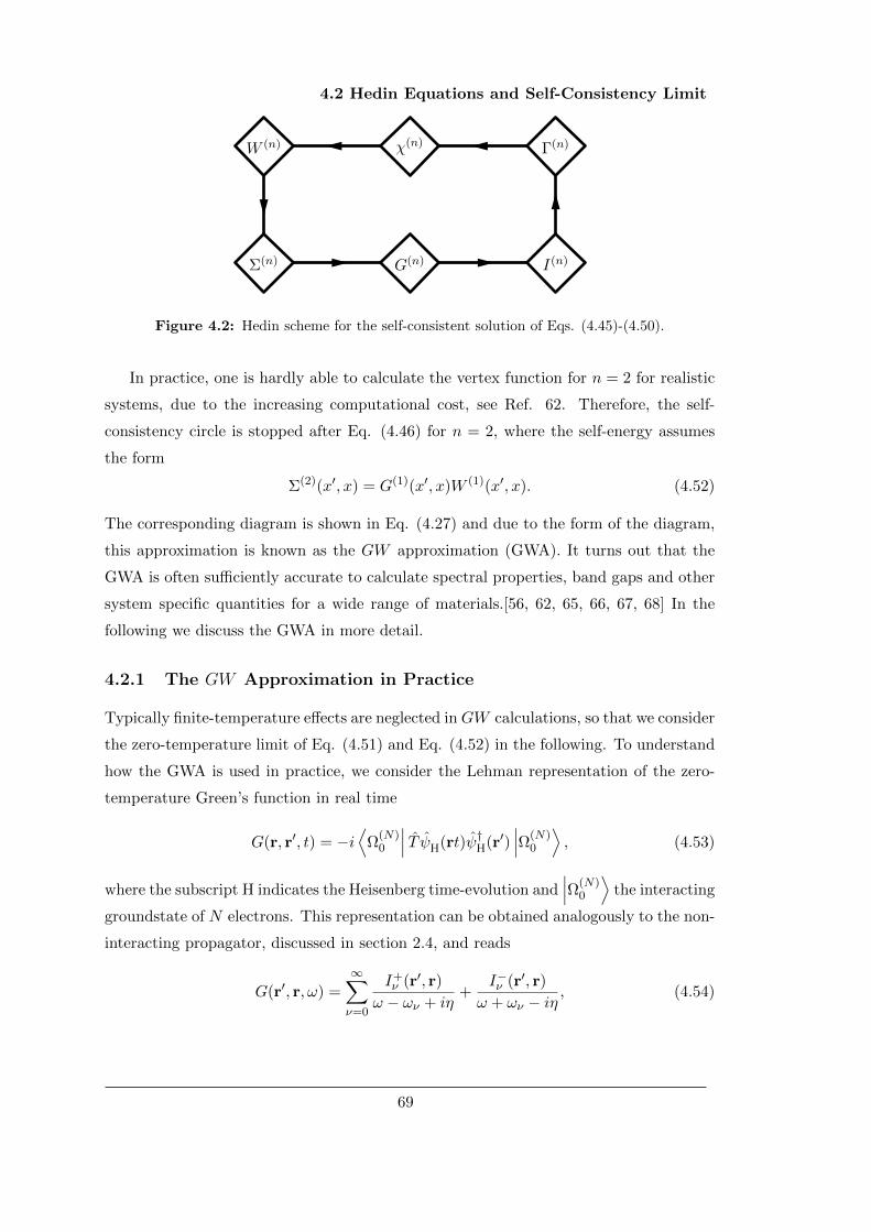
4.2 Hedin Equations and Self-Consistency Limit
Σ(n)
W (n)
I(n)
Γ(n)χ(n)
G(n)
Figure 4.2: Hedin scheme for the self-consistent solution of Eqs. (4.45)-(4.50).
In practice, one is hardly able to calculate the vertex function for n = 2 for realistic
systems, due to the increasing computational cost, see Ref. 62. Therefore, the self-
consistency circle is stopped after Eq. (4.46) for n = 2, where the self-energy assumes
the form
Σ(2)(x′, x) = G(1)(x′, x)W (1)(x′, x). (4.52)
The corresponding diagram is shown in Eq. (4.27) and due to the form of the diagram,
this approximation is known as the GW approximation (GWA). It turns out that the
GWA is often sufficiently accurate to calculate spectral properties, band gaps and other
system specific quantities for a wide range of materials.[56, 62, 65, 66, 67, 68] In the
following we discuss the GWA in more detail.
4.2.1 The GW Approximation in Practice
Typically finite-temperature effects are neglected inGW calculations, so that we consider
the zero-temperature limit of Eq. (4.51) and Eq. (4.52) in the following. To understand
how the GWA is used in practice, we consider the Lehman representation of the zero-
temperature Green’s function in real time
G(r, r′, t) = −i⟨
Ω(N)0
∣∣∣ T ψH(rt)ψ†H(r′)∣∣∣Ω(N)
0
⟩, (4.53)
where the subscript H indicates the Heisenberg time-evolution and∣∣∣Ω(N)
0
⟩the interacting
groundstate of N electrons. This representation can be obtained analogously to the non-
interacting propagator, discussed in section 2.4, and reads
G(r′, r, ω) =∞∑ν=0
I+ν (r′, r)
ω − ων + iη+
I−ν (r′, r)
ω + ων − iη, (4.54)
69

4. SPECTRAL PROPERTIES
with the interacting Lehman amplitudes
I+ν (r′, r) = Θ(ων)
⟨Ω
(N)0
∣∣∣ ψ(r)∣∣∣Ω(N+1)
ν
⟩⟨Ω(N+1)ν
∣∣∣ ψ†(r′) ∣∣∣Ω(N)0
⟩(4.55)
I−ν (r′, r) = Θ(−ων)⟨
Ω(N)0
∣∣∣ ψ†(r′) ∣∣∣Ω(N−1)ν
⟩⟨Ω(N−1)ν
∣∣∣ ψ(r)∣∣∣Ω(N)
0
⟩. (4.56)
and excitation energies given by[35]
ων =
Ω
(N−1)ν − Ω
(N)0 , ων < 0
Ω(N+1)ν − Ω
(N)0 , ων > 0
. (4.57)
It is convenient to introduce the spectral densities
A±(r′, r, ω) =∞∑ν=0
I±ν (r′, r)δ(ω ∓ ων) (4.58)
and to rewrite Eq. (4.54) into
G(r′, r, ω) =
∞∫−∞
dω′[A+(r′, r, ω′)
ω − ω′ + iη+A−(r′, r, ω)
ω − ω′ − iη
], (4.59)
Then the first term of the Lehman representation (4.59) describes the effect of adding
an electron at r′ to a system of N interacting electrons in the groundstate and removing
an electron at r, whereas the second term describes the inverse propagation for a hole.
The same equation shows that the poles of the interacting propagator are all located
along the real axis, so that G has a similar analytic behavior as the non-interacting
propagator G0. In contrast to G0, the Lehman amplitudes cannot be written in terms
of one-electron orbitals φν , i.e.
I+ν (r′, r) 6= φν(r)φ∗ν(r′) 6= I−ν (r′, r). (4.60)
This is because in general the interacting groundstate∣∣∣Ω(N)
0
⟩is not exactly a single
Slater-determinant of the orbitals φν , but rather a linear combination of all possible
determinants, see end of section 1.2. However, often the interacting groundstate of many
systems can be approximated sufficiently accurate by one single Slater-determinant. For
these systems the GWA, as discuss below, is a good approximation.
The first calculations in the GWA have been done by Hybertsen and Louie for semi-
conductors in the 1980s by solving the eigenvalue problem[64]⟨φµ
∣∣∣ h0 + Vh + Σ(2)(εν)∣∣∣φν⟩ = εν
⟨φµ
∣∣∣ φν⟩ (4.61)
70

4.2 Hedin Equations and Self-Consistency Limit
for the quasi particle (qp) one-particle eigensystem∣∣∣φν⟩ , εν. Here h0 is the one-
electron Hamiltonian (2.4), Vh the operator of the Hartree energy (1.16) and Σ(2) the
self-energy operator in the GW approximation with spacetime representation given in
Eq. (4.52). Since the eigensystem of Eq. (4.61) is unknown a priori, Hybertsen and
Louie evaluated the operators h0, Vh, Σ(2) w.r.t. to a DFT one-orbital basis set φν , εν.
Furthermore, they linearized the self-energy w.r.t. to the KS energies εν
Σ(2)(εν) = Σ(2)(εν) +dΣ(2)(ω)
dω
∣∣∣∣∣ω=εν︸ ︷︷ ︸
=Σ′(2)(εν)
(εν − εν) + O((εν − εν)2
), (4.62)
and observed that off-diagonal matrix elements of Eq. (4.61) are negligibly small com-
pared to the diagonal ones, so that they effectively solved⟨φν
∣∣∣h0 + Vh + Σ(2)(εν)− ενΣ′(2)(εν)
∣∣∣φν⟩ = ενZ−1ν (4.63)
for the quasi-particle energies εν . Here the renormalization factor
Zν =1⟨
φν
∣∣∣1− Σ′(2)(εν)∣∣∣φν⟩ (4.64)
typically increases the band gap of the KS system.
It turns out that this scheme, today known as G0W0 approximation, yields often
very good band gap estimates of semiconductors, see Ref. 64. A success of the G0W0
approach motivated researchers to improve the scheme and allow for self-consistent GW
(scGW) calculations. Specifically, the self-consistent scheme of Kotani and Schilfgaarde,
respectively the slightly reformulated approach of Shishkin et al. should be mentioned
at this point, see Refs. 67, 68. In the latter, the eigenvalue equation[h0 + Vh + Σ(2)
(ε(n)ν
)− ε(n)
ν Σ′(2)(ε(n)ν
)] ∣∣∣φ(n+1)ν
⟩= ε(n+1)
ν
[1− Σ
′(2)(ε(n)ν
)] ∣∣∣φ(n+1)ν
⟩(4.65)
is solved iteratively for the one-electron orbitals φ(n)ν and quasi-particle energies ε
(n)ν until
convergence is found. The advantage of this approach is that the resulting self-consistent
solution φν , εν is independent from the initial KS basis φν , εν. This approach is
advantageous for other many-body calculations, where the KS basis does not provide a
good starting point.
71

4. SPECTRAL PROPERTIES
Typically, GW implementations have an O(N4) scaling and, thus, are limited to
rather small systems, see Ref. 67, 68. The bottleneck for these implementations is the
computation of the independent-particle polarizability (4.24) for which the Adler and
Wiser expression of Eq. (3.41) is employed, as for conventional RPA algorithms. The
computational cost of this step can be reduced to O(N3) provided Hedin’s equations
on the imaginary time respectively imaginary frequency axis are used. This approach is
known as the space-time GW approach and was proposed first by Rojas et al. in Ref. 53
and further developed by Steinbeck et al. in Ref. 69 and Ren et al. in Ref. 70. All these
GW approaches, however, face the same storage problem as discussed in section 5.2 for
the RPA algorithm. As a consequence, conventional space-time GW codes avoid solving
the Dyson equation for the propagator (4.46) by assuming implicitly the non-interacting
orbital form of Eq. (2.109) for the propagator in all computation steps.
Using the imaginary time and frequency grids, presented in chapter 5, the storage
problem can be solved and a true O(N3) scaling GW algorithm can be implemented.
This approach has the advantage that the Dyson equation for the propagator can be
solved self-consistently on the GWA level. The corresponding algorithm is currently
investigated and will be presented in a future work.
Nevertheless, the GWA often breaks down for systems with partially filled narrow
bands, for instance transition metal oxides. For these systems an alternative view on the
many-body problem is helpful. For this purpose we introduce the path integral concept
in the following.
72

4.3 The Path Integral
4.3 The Path Integral
The path integral (PI) was introduced by Dirac in the 1930s and extensively developed
by Feynman in the 1940s and is a powerful tool for QFT. It connects the classical prin-
ciple of least action, known from Hamiltonian mechanics, with quantum mechanics and
statistical mechanics. The interested reader is referred to Ref. 71, 72 for a histori-
cal overview, respectively more details about the PI. Here we introduce only the basic
concepts of the PI following closely Negele and Orland, see Ref. 39.
We consider a single particle described by the wavefunction ψ and the Hamiltonian
h(r, p) =p2
2+ ϕ(r), (4.66)
where r denotes the position and p the momentum operator. In the Schrodinger picture
the imaginary time evolution of the corresponding wavefunction ψs from τ = 0 to τ = β
is given by
ψs(r, β) =
∫dr′ 〈r| e−βh(r′,p)
∣∣r′⟩ψ(r′). (4.67)
We slice the time path from 0 to β into M equidistant pieces according to
δτ =β
M, τi = iδτ, i = 0, · · · ,M (4.68)
and introduce the notation
ri = r(τi), r0 = r′, rM = r (4.69)
with the eigenvalue equation for the position operator
r |ri〉 = ri |ri〉 (4.70)
Applying this subdivision to Eq. (4.67) and inserting the closure relation
1 =
∫dri |ri〉 〈ri| , (4.71)
one ends up with
ψs(r, β) =
∫ M∏i=0
dri 〈r| e−δτh(rM−1,p) |rM−1〉 · · · 〈r1| e−δτh(r0,p)∣∣r′⟩ψ(r′) (4.72)
73

4. SPECTRAL PROPERTIES
Any expectation value on the r.h.s. can be rewritten as follows
〈ri+1| e−δτh(ri,p) |ri〉 = 〈ri+1| ri〉︸ ︷︷ ︸δ(ri+1−ri)
e−δτh(ri,pi)
=
∫d3pi(2π)3
eδτ(pi
ri+1−ri−iδτ −h(ri,pi)
), (4.73)
where in the first step we used the real-space representation pi = −i∇i and the integral
representation for the Dirac delta distribution.
Defining the limits r(τi) = limδτ→0
ri+1−ri−iδτ , the abbreviation
∫τ =
∫ β0 dτ and the PI
measure
D[r(t),p(t)] = limM→∞
M∏i=0
d3rid3pi
(2π)3, (4.74)
one obtains for Eq. (4.72) in the limit M →∞
ψs(r, β) =
r(β)=r∫r(0)=r′
D[r(t),p(t)]e∫τ [p(τ)r(τ)−h(r(τ),p(τ))]ψ(r). (4.75)
This expression 4.75 is known as the Hamiltonian form of the path integral.[39, 47] If
the Gaussian integral formula (C.2) is used to carry out the integration over momenta
pi, one ends up with the corresponding Lagrangian form[39]
ψs(r, β) =
r(β)=r∫r(0)=r′
D[r(t)]eSclass[r(τ),r(τ)]ψ(r), (4.76)
where the classical action
Sclass[r(τ), r(τ)] =
∫τ
r2(τ)
2− ϕ [r(τ)]
(4.77)
appears in the exponent of Eq. (4.76).
The last two expressions are intriguing, since they show that the propagation of
a quantum particle from state ψs(r′, 0) to ψs(r, β) is determined by the sum over all
classical paths between the spacetime points (r′, 0) and (r, β). Furthermore, the path
integral allows to bridge the gap to statistical physics, since the partition function of the
system can be written elegantly as
z(β) =
∫d3r 〈r| e−βh |r〉 =
∫r(0)=r(β)
D[r(τ),p(τ)]e∫τ [p(τ)r(τ)−h(r(τ),p(τ))]. (4.78)
74
4.3 The Path Integral
Here, we emphasize that only periodic paths r(0) = r(β) in the phase space contribute
to z(β).
One can show, see Ref. 39, that the path integral carries the time-ordering sym-
bol T intrinsically in its definition, so that thermal expectation values of time-ordered
observables O(r(τ)) are given by
TrTO1(r, τ1)O2(r, τ2)e−βh
Tre−βh
=
∫D[r(τ)]O1(r(τ1))O2(r(τ2))eS[r(τ),r(τ)]∫
D[r(τ)]eS[r(τ),r(τ)](4.79)
Here the trace on the l.h.s. indicates a sum over the position eigenstates.
4.3.1 Path Integral for Quantum Fields
So far we have considered a single particle. In the following, we concentrate ourselves to
quantum fields, starting with bosonic fields φ, which satisfy the canonical commutation
relations [φ†(r, τ), φ(r′, τ)
]= iδ(r− r′). (4.80)
In this case, the path integral (4.75) is generalized straightforwardly by applying the
rules of first quantization
p(τ)→ iφ∗(τ), r(τ)→ φ(τ), r =∂r
∂t→ i
∂φ
∂τ(4.81)
in Eq. (4.75) obtaining the grand canonical partition function of bosonic QFT[39]
Zb(β) =
∫φ(0)=φ(β)
D[φ(τ), φ∗(τ)]e−∫τ [φ∗(τ)( ∂∂τ )φ(τ)+H(φ∗(τ),φ(τ))]. (4.82)
Here H(φ(τ), φ∗(τ)) is the corresponding Hamiltonian of the considered bosonic QFT
and the notation φ(τ) =∫
d3rφ(r, τ) is used.
However, we are interested in the fermionic case, where the electronic field operators
ψ, ψ†, satisfy anticommutation rules (2.26) rather than Eq. (4.80). As a consequence, the
fermionic analogue of (4.82) has to be defined, such that the antiperiodicity of the trace,
see Eq. 2.115, is taken into account. This is achieved by introducing Grassmann fields
ψ(τ), ψ∗(τ) with antiperiodic boundary conditions ψ(0) = −ψ(β). A short introduction
of the Grassmann algebra is given in appendix C.1 and more details can be found in
Refs. 39, 47.
75

4. SPECTRAL PROPERTIES
Within this algebra the electronic path integral assumes the same form as for bosons,
with the difference that the PI variables φ, φ∗ are replaced by ψ,ψ∗ and reads
Z(β) =
∫ψ(0)=−ψ(β)
D[ψ(τ), ψ∗(τ)]e−∫τ [ψ∗(τ)( ∂∂τ +h)ψ(τ)+V (ψ∗(τ),ψ(τ))]. (4.83)
Here, H = H0 + V was used in combination with the field representation of the non-
interacting and interacting Hamiltonians (2.2) and (2.3).
In analogy to chapter 3, the expansion of the factor e−∫τ V into a series generates the
perturbation series of the partition function and the same diagramatic tools as in chapter
3 can be used within the PI formalism. For this purpose, we introduce the notation⟨⟨O(r′, τ ′)
⟩⟩β
=1
Z0(β)
∫D[ψ(τ), ψ∗(τ)]O(r′, τ ′)e−
∫τ ψ∗(τ)( ∂∂τ +h)ψ(τ) (4.84)
to indicate thermal averaging in terms w.r.t. to the non-interacting system, such that
Z(β) =⟨⟨e−∫τ V⟩⟩
β(4.85)
holds. This notation should be contrasted to the conventional notation 〈·〉β defined in
Eq. (2.112).
Following the discussion in section 2.7.2, the generating functional W[j, j∗], defined
in Eq. (2.135), can be written in the PI formalism as
W[j, j∗] = ln
⟨⟨e−∫τ [V (τ)+j∗(τ)ψ(τ)+ψ∗(τ)j(τ)]
⟩⟩β
. (4.86)
Here j, j∗ indicate Grassman source fields, which are set to zero after differentiation. For
instance the interacting Green’s function G reads
G(x1, x2) = − δ2W[j∗, j]
δj(x1)δj∗(x2)
∣∣∣∣j∗,j=0
, xi = (ri, τi) (4.87)
whereas more general correlation functions can be obtained from
G(x1 · · · , xn, x′1, · · · , x′n) = (−1)nδ2nW[j∗, j]
δj(x1) · · · δj(xn)δj∗(x′1) · · · j∗(x′n)
∣∣∣∣j∗,j=0
. (4.88)
In the following we use the PI to gain an alternative perspective on the many-body
problem in terms of effective Hamiltonians, which describe only a small subset of the full
Fock space F. The corresponding effective Hamiltonian can be obtained after specific
degrees freedom of the system are integrated out. For instance integrating out all non-
local degrees yields a purely local effective Hamiltonian, which describes only a small set
of states localized on specific atoms. This is the topic of the following section. For this
purpose it is convenient to consider the many-body Hamiltonian in a localized basis set.
76

4.4 Effective Hamiltonians
4.4 Effective Hamiltonians
In this section we consider the many-body problem from a localized point of view. Our
aim is to derive an effective interaction Seff , where all degrees of freedom are integrated
out, except those at R = 0. For this purpose we closely follow Ayral et al.[73] and use
the cavity method described in Ref. 74.
4.4.1 The Many-Body problem in the Wannier Basis
As a starting point, we consider a localized basis set |wα〉 containing a site index α and
a real lattice vector index Rα by bold Greek indices α = (α,Rα), i.e.
〈r |wα〉 = wα(r−Rα) (4.89)
Similarly α = (α,Rα = 0) denotes local and α = (α,Rα 6= 0) non-local states, that
is states not centered at Rα = 0. The states |wα〉, known as Wannier states and
are obtained from the Bloch states |φnk〉 by an unitary transformation T(k)nα with an
additional discrete Fourier transformation[75]
|wα〉 =1
Nk
∑nk
eikRαT (k)nα |φnk〉 . (4.90)
Here Nk represents the number of k-points in the first Brillouin zone. We discuss the
construction of Wannier states in section 6.1 in more detail. Here, we only use the
fact, that field operators can be decomposed into Wannier states (Einstein summation
convention)
ψ(r) = wα(r)dα, dα =
∫drw∗α(r)ψ(r), (4.91)
using the annihilation operator in the Wannier basis
dα =1
Nk
∑nk
eikRαT (k)nα cnk. (4.92)
Within this notation and the definitions of the hopping and the Coulomb interaction
matrix
tαβ = 〈wα| h |wβ〉 (4.93)
Vαβγδ = 〈wα, wβ| V |wδ, wγ〉 , (4.94)
77

4. SPECTRAL PROPERTIES
the normal-ordered many-body Hamiltonian H in the interaction picture reads
H(τ) = tαβd†α(τ)dβ(τ) +1
2V αβγδd†α(τ)d†β(τ)dγ(τ)dδ(τ). (4.95)
In the following we assume that the Wannier states are sufficiently localized in real space,
such that
Vαβγδ ∝ δ(Rα −Rδ)δ(Rβ −Rγ) (4.96)
is a reasonable approximation.
It is convenient to use the anticommutation rules1
d†α, dβ
= δαβ, (4.97)
to rewrite the Wannier Hamiltonian (4.95) into the density form
H(τ) = kαβnαβ(τ) +1
2V αβγδnαδ(τ)nβγ(τ) (4.98)
by absorbing the exchange term −12V
αγβγ into the hopping matrix
kαβ = tαβ − 1
2V αγβγ (4.99)
and using the number (or density) operator in the Wannier representation
nαδ = d†αdδ. (4.100)
We emphasize, that there is a variety of different rearrangements of the operators in the
interaction term. For instance, one can absorb the Hartree term V αβ δβ in the hopping
matrix instead, see Ref. 39. However, for reasons that will become clear later on and to
be compatible with the assumption made in Eq. (4.96), we choose the rearrangement
defined in Eqs. (4.98) and (4.99).
4.5 Local effective Hamiltonians
The Wannier representation (4.98) of the Hamiltonian H defines a path integral
Z(β) =
∫D [d, d∗] e−S[d,d∗], (4.101)
1 This is a consequence from Eq. (4.92) being a unitary transformation and the canonical anticom-
mutation rules Eq. (2.26).
78

4.5 Local effective Hamiltonians
with antiperiodic Grassmann variables dα(τ + β) = −dα(τ). Here, the full many-body
action S = S0 + Sv is divided into a non-interacting S0 and interacting action Sv, given
by
S0[d, d∗] =
∫τd∗α(τ)
[G−1
x (τ)]αβ
dβ(τ) (4.102)
Sv[d, d∗] =
1
2
∫τd∗α(τ)dδ(τ)V αβγδd∗β(τ)dγ(τ). (4.103)
For future reference, the exchange Green’s function is introduced
[G−1
x (τ)]αβ
=[δαβ∂τ − kαβ
](4.104)
in analogy to the non-interacting propagator G0, see section 2.4.
To integrate over all non-local Grassman fields d∗α, dβ, we use the bosonic variables
nαβ = d∗αdβ with periodic boundary conditions nαβ(τ + β) = nαβ(τ). The latter prop-
erty allows for a Hubbard-Stratonovich transformation of the kind (C.15) to decouple
the interaction term e−Sv in Eq. (4.101), to obtain
Z(β) ∝∫
D [d, d∗, φ] e−S[d,d∗,φ] (4.105)
with
S[d, d∗, φ] =
∫τd∗α(τ)
[G−1
x (τ)]αβ
dβ(τ)
+1
2
∫τφαδ(τ)
[V −1
]αβγδφβγ(τ) + i
∫τφαβ(τ)nαβ(τ). (4.106)
using the auxiliary real-valued bosonic fields φαβ(τ).[76]
In the next step, one splits this action into three parts, a local
Sloc[d, d∗, φ] =
∫τd∗α(τ)
[G−1
x (τ)]αβ
dβ(τ)
+1
2
∫τφαδ(τ)
[V −1
]αβγδφβγ(τ) + i
∫τφαβ(τ)nαβ(τ), (4.107)
a non-local
Snloc[d, d∗, φ] =
∫τd∗α(τ)
[G−1
x (τ)]αβ
dβ(τ)
+1
2
∫τφαδ(τ)
[V −1
]αβγδφβγ(τ) + i
∫τφαβ(τ)nαβ(τ), (4.108)
79

4. SPECTRAL PROPERTIES
and a mixed term
Smix[d, d∗, φ] = −∫τtαβ[d∗α(τ)dβ(τ) + d∗β(τ)dα(τ)
]+
∫τφαδ(τ)
[V −1
]αβγδφβγ(τ) (4.109)
by appropriately restricting the summation over Wannier statesα into local α = (α,Rα 6=0) and non-local states α = (α,Rα = 0) respectively. In arriving at Eqs. (4.107)-(4.109)
Eq. (4.96) was used, which implies both, kαβ = tαβ and φβγnβγ = 0, and reveals the
reason of the rearrangement in the Hamiltonian (4.98). Furthermore, the last term of
Eq. (4.109) was obtained using the relation
1
2φαδ(τ)
[V −1]αβγδ
+[V −1
]βαδγ︸ ︷︷ ︸[V −1]αβγδ
φβγ(τ) = φαδ(τ)[V −1
]αβγδφβγ(τ). (4.110)
Now the auxiliary fermionic and bosonic field variables
ηβ(τ) = tαβdα(τ) (4.111)
ζ βγ(τ) = φαδ(τ)[V −1
]αβγδ(4.112)
are introduced and the mixed term (4.109) is rewritten into
Smix[d, d∗, φ, η∗, η, ζ] = −∫τ
[η∗β(τ)dβ(τ) + d∗β(τ)ηβ(τ)
]+
∫τζ βγ(τ)φβγ(τ). (4.113)
This expression reveals, that Smix contains all fermionic and bosonic source fields for a
system with a cavity at R = 0. Hence, in analogy to Eq. (4.88) and Eq. (4.86) the
corresponding generating functional W[η∗, η, ζ] for all connected fermionic and bosonic
Green’s functions of the system (with a cavity) is given by
W[η∗, η, ζ] = ln
∫D [d∗, d, φ]|R6=0 e
−Snloc[d∗,d,φ]−Smix[d∗,d,φ,η∗,η,ζ] (4.114)
and the corresponding interacting correlation functions are obtained as derivatives
Gα1···βn(τ1, · · · , τ ′n) = (−1)nδ2nW[η∗, η, 0]
δη∗α1(τ1) · · · δη∗αn(τ ′n)δηβn(τ ′n) · · · δηβ1
(τ ′1)
∣∣∣∣∣η,η∗=0
(4.115)
W α1···βn(τ1, · · · , τ ′n) =1
2nδ2nW[0, 0, ζ]
δζα1δ1(τ1) · · · δζαnδn(τ ′n)δζβnγn(τ ′n) · · · δζβ1γ1
(τ ′1)
∣∣∣∣∣ζ=0
.(4.116)
80

4.5 Local effective Hamiltonians
We emphasize that G and W is the propagator, respectively the effective interaction, of
a system with removed primitive cell at R = 0. Alternatively, one obtains G and W via
the PIs
Gα1···βn(τ1, · · · , τ ′n) =
∫D[d∗, d]|R6=0dα1(τ1) · · · d∗
βn(τ ′n)e−Snloc−Smix∫
D[d∗, d]|R6=0e−Snloc−Smix(4.117)
W α1···βn(τ1, · · · , τ ′n) =1
2n
∫D[φ]|R6=0φα1δ1
(τ1) · · ·φβnγn(τ ′n)e−Snloc−Smix∫D[φ]|R6=0e−Snloc−Smix
(4.118)
These correlation functions must not be confused with the correlation functions G,W
of the full system.[74]
On the one side, Eqs. (4.115) and (4.116) imply an explicit expression for the cavity
functional (4.114) in terms of correlation functions
W[η, η∗, ζ] =
∞∑n=1
(−1)n∫τ1
· · ·∫τ ′n
η∗α1(τ1) · · ·Gα1,···βn(τ1, · · · , τ ′n)ηβ1
(τ ′1) · · ·
+∞∑n=1
1
2n
∫τ1
· · ·∫τ ′n
ζα1δ1(τ1) · · ·W α1β1,···γnδn(τ1, · · · , τ ′n)ζβ1γ1
(τ ′1) · · · .
(4.119)
On the other side, Eqs. (4.111), (4.112) show that W[η, η∗, ζ] depends only on local
variables dα, d∗β and φαβ, so that the integration over all non-local states in the partition
function (4.105) can be carried out and yields an factor eW[η,η∗,ζ] in the same path
integral.
The resulting expression has only local terms, so that the partition function of the
complete system reads
Z(β) ∝∫
D[d, d∗, φ]|R=0 e−Seff [d,d∗,φ,η,η∗,ζ] (4.120)
and contains the effective local action Seff , we are looking for
Seff [d, d∗, φ, η, η∗, ζ] = Sloc[d, d∗, φ]−W[η, η∗, ζ]. (4.121)
Finally the φ-integration can be evaluated with the inverse Hubbard-Stratonovich trans-
formation (C.15) and one obtains for the partition function
Z(β) =
∫D[d, d∗]|R=0 e
−Seff [d,d∗]. (4.122)
81
4. SPECTRAL PROPERTIES
Here the effective action
Seff [d, d∗] =
∫τ1
∫τ ′1
d∗α(τ1)[G−1
]αβ(τ1 − τ ′1)dβ(τ ′1)
+1
2
∫τ1
∫τ ′1
nαδ(τ1)Uαβγδ(τ1 − τ ′1)nβγ(τ ′1) (4.123)
contains the correlation functions[G−1
]αβ(τ1 − τ ′1) =
[G−1
x (τ1 − τ ′1)]αβ
− tαµ1[Gµ1ν1(τ1 − τ ′1) + · · ·
]tβν1 (4.124)[
U−1]αβγδ
(τ1 − τ ′1) =[V −1
]αβγδδ(τ1 − τ ′1)
−[V −1
]αµ1ν1δ
[W
µ1β1γ1ν1(τ1 − τ ′1) + · · ·] [V −1
]β1βγγ1
,(4.125)
where the dots indicate terms of Eq. (4.119) with n > 1.
Expression (4.123) has the form of an impurity model, where the impurity cell is
located at R = 0 and interacts with an effective, surrounding medium. This medium
is described by the cavity correlation functions G and W , appearing on the r.h.s. of
Eqs. (4.124) and (4.125). These cavity functions correct the local exchange Green’s
function Gαβx and the local bare Coulomb interaction Vαβγδ of the lattice, yielding the
non-interacting impurity propagator Gαβ(τ), respectively the bare impurity interaction
Uαβγδ(τ). The latter describes the interaction between impurity states, whereas the
former can be seen as an undressed propagation from site β to site α. The corresponding
dressed propagation,i.e. the interacting Green’s function of the impurity can be obtained
as a path integral
[Gimp]αβ(τ) =⟨⟨dα(τ)d∗β
⟩⟩= −
∫D[d, d∗]|R=0 dα(τ)d∗βe
−Seff [d,d∗]∫D[d, d∗]|R=0 e
−Seff [d,d∗]. (4.126)
We emphasize that [Gimp]αβ is both, the interacting Green’s function of the impurity
model (4.123), as well as the interacting Feynman propagator Gαβ of the full many-body
Hamiltonian (4.98) restricted to the unit cell R = 0. Similar arguments hold for the
dressed impurity interaction Wimp and W , see Ref. 73, so that, we deduce effective
Dyson equations for the impurity model (4.123)
Gαβ(iωn) = Gαβ(iωn) + Gαγ(iωn)Σγδimp(iωn)Gδβ(iωn) (4.127)
Wαβγδ(iνn) = Uαβγδ(iνn) + Uαµνδ(iνn)χνµρσimp (iνn)Wρβγσ(iνn). (4.128)
82

4.5 Local effective Hamiltonians
Here Σimp is the effective, irreducible self-energy and χimp the corresponding bosonic
counterpart (irreducible polarizability) of the impurity model. Since the former is a
fermionic and the latter a bosonic quantity, ωn represents fermionic and νn bosonic
Matsubara frequencies.[73] The fermionic and bosonic self-energies Σimp and χimp differ
from the lattice self-energies Σ and χ, because the non-interacting fermionic and bosonic
propagators G and U of the impurity model differ from G0, respectively V [see (4.124),
(4.125)].
However, one can show that in the limit of infinite dimensions d → ∞, the self-
energies of the impurity coincide with the local self-energies of the full many-body
Hamiltonian H
limd→∞
[Σimp]αβ = Σαβ (4.129)
limd→∞
[χimp]αβγδ = χαβγδ. (4.130)
The first limit is the starting point of dynamical mean field theory (DMFT), whereas
the inclusion of the second limit is used in extended DMFT (eDMFT). In the following
we concentrate ourselves on DMFT, more about eDMFT can be found in Ref. 73.
4.5.1 Dynamical Mean Field Theory
We consider standard DMFT in this section, which is traditionally formulated for the
Hubbard model. Within this model the hopping matrix tαβ is restricted to nearest
neighbors, which we indicate by the symbol t<αβ> in the following. Originally, the
Hubbard model takes only static interactions between opposite spins on the same site
into account, see Ref. 77. However, we allow for additional interactions and consider
the following model
Hmod = t<αβ>d†αdβ +1
2V αββαnααnββ, (4.131)
where the interactions are restricted to the unit cell.
Despite of its simplicity, it turns out that the Hubbard model has a rich phase diagram
and describes a vast number of physical phenomena, including Mott-Hubbard transitions,
the Kondo effect and many kinds of magnetism, see Ref. 78 for an introduction with
selected results. These phenomena stem mostly from partially filled narrow bands around
the Fermi surface, which demand an accurate description of correlation effects beyond
83
4. SPECTRAL PROPERTIES
the mean-field (DFT or HF) or even the GWA level. Therefore, one characterizes these
systems as strongly correlated and often tries to describe them by applying a model of
the Hubbard form (4.131).
However, the attempt to solve (4.131) (or similar models) for d = 3 dimensions often
fails, due to the high dimension of the corresponding Hilbert space. In fact, today only
for d = 1 and one single Wannier state the Hubbard model can be solved analytically, see
Refs. 79, 80. Metzner and Vollhardt tackled this problem not from the low-dimensional,
but from the high-dimensional limit, see Ref. 81. They considered the Hubbard model
for d → ∞ dimensions and showed that a non-trivial limit of Eq. (4.131) is obtained if
the hopping amplitude is scaled simultaneously according to
tαβ →1√zdtαβ, (4.132)
where zd ∈ O(d) is the coordination number of the lattice in d dimensions and tαβ finite
for d→∞.1 In the case of our model, defined in Eq. (4.131), the second term has to be
scaled as well
V αββγ → 1
zdV αββγ (4.133)
(with finite V ) to yield a non-trivial limit for d→∞, see Ref. 82.
Simple power counting arguments can be used, see Ref. 82, to show that only the first
term in the [·]-brackets of Eqs. (4.124) and (4.125) survive for d → ∞. Consequently,
the effective action Seff of Eq. (4.123) for the model (4.131) in the limit d→∞ assumes
the form
S∞[d, d∗] = limd→∞
Seff [d, d∗]
=−∫τ
[∫τ ′d∗α(τ)
[G−1
]αβ(τ − τ ′)dβ(τ ′) +
1
2nαδ(τ)Uαβγδnαδ(τ)
] (4.134)
with the Weiss field (4.124) given by
[G−1
]αβ(τ − τ ′) = δ(τ − τ ′)δαβ∂τ − tαµ Gµν(τ − τ ′)tβν , (4.135)
This result follows from t<αβ> = 0 and the fact that the Hubbard model (4.131) already
has the density form of (4.98).
1 This scaling relation follows from the fact that the density of states for V = 0 and d→∞ is finite,
see Ref. 81.
84

4.5 Local effective Hamiltonians
This expression simplifies on the Matsubara axis iωn,[G−1
]αβ(iωn) = δαβiωn − tαµ Gµν(iωn)tβν (4.136)
Furthermore, using simple power counting arguments, see Ref. 74, the cavity Green’s
function can be related to the local lattice propagator G via
Gµν = Gµν(iωn)−Gµγ(iωn)[G−1(iωn)
]γδGδν(iωn), (4.137)
which finally results after rewriting Eq. (4.136), see Ref. 73, in[G−1(iωn)
]αβ
=[G−1(iωn)
]αβ
+ Σαβ(iωn). (4.138)
This expression reveals the connection between a fictitious impurity model located at
R = 0 (and determined by G and U) and the Hubbard model determined by the renor-
malized Feynman propagator G and its self-energy Σ. This relationship is exact only
in the limit of infinite dimensions. However, it turns out that the identification of the
interacting Green’s function of the impurity with the local interacting Green’s function
of the lattice is an excellent approximation for strongly correlated systems in finite di-
mensions, like d = 3.[81] Therefore, Eq. (4.138) is exploited in practice to solve the
Hubbard model in finite dimensions by determining the Weiss field G in Eq. (4.138)
self-consistently. This can be done using following algorithm
DMFT Algorithm
D1 Start with some initial guess for the Weiss field G and choose a fixed impurity
interaction U.
D2 Compute the impurity propagator Gimp with Eq. (4.126) for the action (4.134)
and extract its self-energy with Σimp = G−1−G−1imp. This self-energy approximates
the local self-energy of the Hubbard model.
D3 Compute the interacting propagator G of the lattice with G−1 = Σ +G−10 , where
G0 is the non-interacting Green’s function of the Hubbard model.
D4 The resulting propagator of D3 is used to determine a new estimate for the Weiss
field via G−1 = Σimp +G−1.
D5 Iterate D2-D4 until∣∣G(n+1) − G(n)
∣∣→ 0.
85

4. SPECTRAL PROPERTIES
This algorithm yields a good estimate for the interacting Green’s function of the Hubbard
model. However, the Hubbard model cannot describe the physics of real materials in any
detail. Heuristically speaking, DMFT describes only local correlation effects and fails
in general to capture non-local many-body effects. Realistic approaches, on the other
hand, have to take into account both, local and non-local correlations.
For this purpose the LDA+DMFT method was developed, see Ref. 83 for a com-
prehensive overview. Within LDA+DMFT the interacting Green’s function G (used in
step D3) is computed from the KS hopping matrix
t(k)αβ = T (k)
αn εnkT(k)βn . (4.139)
via [G−1(iωn)
]αβ
=1
Nk
∑k
[(iωn + µ)δαβ − t(k)
αβ − Σαβ(iωn) + (tdc)(k)αβ
]. (4.140)
Here Σαβ(iωn) is the local self-energy of the impurity given on the Matsubara axis ωn,
µ the chemical potential and (tdc) the double-counting correction.[84] The last term is
present, due to the fact that the LDA (or any other KS) hopping matrix t(k)αβ contains local
correlation terms, which are also included in the local self-energy Σαβ(iωn). In the ideal
case, these terms are described by (tdc)(k)αβ , however, in practice this term is unknown,
because of the non-diagrammatic nature of DFT. This issue is known as double counting
problem and is typically treated by approximating (tdc)(k)αβ = µdcδαβ and absorbing the
term into the chemical potential. More about the (ambiguous) computation of µdc is
found in Refs. 85, 86 and will not be considered here.
In the following, we follow a more promising route, the combination of the GW with
the DMFT approximation. The reason for this is that in GW+DMFT, studied first
by Biermann et al. in their seminal paper [87], both approaches can be formulated in
the diagrammatic language. This has the advantage that, on the one side, the double
counting terms can be identified in principle unambiguously within GW+DMFT. On
the other side, the GW formalism can be used to determine the effective interaction
matrix U of the impurity model (4.134) and is discussed in detail in section 6.1.3.
86
Part II
Methodological Developments
87


5
Low Scaling Algorithm for the
Random Phase Approximations
The following chapter presents an efficient zero-temperature RPA algorithm, which scales
cubicly with the number of electrons N in the system. To keep the notation simple in
this chapter, we write G instead of G0 for the non-interacting Green’s function, χ for the
independent-particle polarizability χ0 and suppress the imaginary unit i in the frequency
arguments of χ. Furthermore, to avoid confusion we use χ to indicate the imaginary
time polarizabilities.
The following chapter was published in Refs. 88 and 89.
5.1 Computational Scheme
We have implemented an RPA algorithm for periodic systems at zero-temperature,1
which is summarized by the flow diagram shown in Fig. 5.1. This figure shows that the
ACFDT formula Eq. (3.37) is only the last step in the calculation of the RPA correlation
energy ERPAc . The evaluation of this step was presented in Ref. 90 and will not be dis-
cussed in this thesis. Here, we concentrate on the preceding steps, which are technically
more demanding. We discuss each step of Fig. 5.1 in detail in reverse order starting
with the cosine transformation (CT) of χ from imaginary time to imaginary frequency
1Finite-temperature effects are not considered here, but can be included easily by using finite-
temperature Green’s functions.
89

5. LOW SCALING ALGORITHM FOR THE RANDOM PHASEAPPROXIMATIONS
FFT
CT
FFT
GG
ACFDTERPA
c
Gk(g,g′, τ)
χk(g,g′, τ)
χ(r, r′, τ)G(r, r′, τ)
χk(g,g′, ν)
Figure 5.1: Calculation scheme for the RPA correlation energy ERPAc adopted in this paper.
The first and third step is a spatial fast fourier transformation (FFT) described in Sec. 5.3.
The second step is the contraction of two Green’s functions in the space-time domain (GG)
giving the independent-particle polarizability χ (see Sec. 5.4). The cosine transformation
(CT) in the fourth step is described in Sec. 5.2.3. The ACFDT is formulated in Eq. (3.37).
in section 5.2. The fast fourier transformation (FFT) of χ from real to reciprocal space
is discussed in section 5.3 followed by the contraction step (GG) in section 5.4.
5.2 Imaginary Time and Frequency Grids
The following section was published in Ref. 88.
The forth step of the RPA algorithm, denoted as CT, is the transformation of the
polarizability χ0k(g,g′, τ) to the imaginary frequency domain χ0
k(g,g′, ν). For an accu-
rate discrete Fourier transformation, an equally spaced grid for the time and frequency
domain necessitates a few hundred grid points, see Ref. 69. This makes the calculations
rather expensive, so that the break even point between the traditional O(N4) algorithm
and the lower scaling O(N3) algorithm is reached only for very large systems. Such large
systems are then also difficult to handle, since the storage demands for the polarizability
at many frequency points can easily exceed the available memory even on modern large
scale computers. This implies that the approach can be applied to large systems only if
the number of grid points τi, νk, which are needed for an accurate representation of the
functions χ0k(g,g′, τ) and χ0
k(g,g′, ν), as well as their Fourier transformation, is kept as
small as possible.
90

5.2 Imaginary Time and Frequency Grids
In this section, we first determine tailor-made quadratures for the direct second or-
der Møller-Plesset (MP2) energy in the imaginary frequency domain (as opposed to
the usual imaginary time domain used in the Laplace-transformed MP2 (LT-MP2)
method.[91]). Apart from comparing the Minimax and least square quadratures for
the LT-MP2 method, we show that our frequency grid is also able to integrate the RPA
correlation energy accurately using ≈ 16 quadrature points. In addition, approximat-
ing the Fourier integral of the polarizability by means of a quadrature formula, we find
an elegant method to switch from imaginary time to imaginary frequency polarizabili-
ties (and vice versa) without using an interpolation technique or significantly increasing
the number of grid points. This allows to evaluate RPA energies with well-controlled
approximations (time and frequency grids) with O(N3) scaling.
The section is organized as follows. In section 5.2.1 and 5.2.2 we review the necessary
mathematical background for tailor-made quadrature formulas. In section 5.2.3, we
present a method for the accurate determination of the cosine integral of χ in terms of
the imaginary time counterpart χ. In section 5.2.5 and 5.2.6 we compare the convergence
behavior of the Minimax and least square quadratures for MP2 and RPA calculations.
In addition, results for RPA and direct MP2 energies using the non-uniform cosine
transformation established in 5.2.3 are given in section 5.2.5 and 5.2.6.
5.2.1 The Fitting Problem
Given a function f : I = [1, R] → R with R > 1 and a model function y : R × I → R,
the fitting problem is stated as follows: find the set of coefficients α = (α1, · · · , αn),β =
(β1, · · · , βn) ∈ Rn such that the error function
η(α,β, ξ) = f(ξ)−n∑i=1
βiy(αi, ξ) (5.1)
is minimal with respect to one of the following norms
‖η‖2 =
∫ R
1dξ |η(α,β, ξ)|2 (5.2)
‖η‖∞ = max |η(α,β, ξ)| ∈ R : ξ ∈ I . (5.3)
Minimization w.r.t. ‖ · ‖2 gives the least square (LS) coefficients α0 and β0. The corre-
sponding fit minimizes the average or mean error, but results in an uneven distribution
of the error in the interval I, with errors depending on the distribution of the points ξ.
91

5. LOW SCALING ALGORITHM FOR THE RANDOM PHASEAPPROXIMATIONS
A possible way of computing α0 and β0 for non-linear fitting problems is the Levenberg-
Marquardt algorithm, see Ref. 92, or the variable projection algorithm of Golub and
Pereyra.[93] In this work we use exclusively the latter method.
On the other side, minimizing η w.r.t. ‖ · ‖∞ gives the so called Minimax (MM)
solution α∗,β∗.[94] This means that the maximum error is minimized and the error
is consequently equally distributed inside the interval I. Usually this is desired if the
distribution of the ξ points is unknown. Note that throughout this paper we will always
use an asterisk, α∗i , β∗i , when referring to grids and weights corresponding to Minimax
solutions, whereas the conventional least square grids will carry the superscript 0.
Implementations calculating α∗,β∗ use typically the Remez algorithm, which re-
lies on Chebyshev’s alternation theorem.[95] This theorem states that in the Minimax
approximation the error function satisfies
η(α∗,β∗, ξj) = (−1)jε, ∀j = 1, · · · , 2N + 1, ε > 0 (5.4)
where the points ξj are the local extrema of η. In total there are 2N + 1 minima and
maxima leading to 2N + 1 linear independent equations (5.4): 2N equations for the
coefficients α,β and one for the minimized error extremum ε.
Assuming we have a starting guess (say α0 and β0) for the coefficients, we can apply
the Remez algorithm:
R1 Find all extrema ξj2N+1j=1 of η.
R2 Solve (5.4) for α,β and ε at the determined extrema ξj .
R3 Update coefficients and error α,β and ε.
R4 Iterate R1-R4 until convergence.
The solution of the fitting problem can be used in order to find optimal quadrature
formulas for the numerical evaluation of integrals. In the following, we discuss the
application for integrals appearing in RPA and MP2.
92

5.2 Imaginary Time and Frequency Grids
5.2.2 Integral Quadrature Formulas for RPA and Direct MP Energies
We are interested primarily in the numerical evaluation of the RPA correlation energy
at zero-temperature given in Eq. (3.37). To keep notation simple we write χ for χ0 and
focus ourselves only on the frequency, respectively the time dependence of the indepen-
dent particle polarizability. Furthermore the trace symbol in (3.37) will be suppressed
in this chapter.
The lowest contribution (n = 2) to the RPA is the direct MP2 correlation energy
and reads[96, 97]
E(2)c =
1
8π
∞∫−∞
dν χ(ν)V 2 . (5.5)
Instead of evaluating this integral in the imaginary frequency domain, we can insert the
Fourier transformation
χ(ν) =
∫ ∞−∞
dτ χ(τ)eiντ (5.6)
into Eq. (5.5) and use∫
dνe±iν(τ+τ ′) = 2πδ(τ + τ ′) in order to obtain the corresponding
imaginary time representation
E(2)c =
1
4
∫ ∞−∞
dτχ(τ)V 2. (5.7)
This expression is the Laplace transformed direct MP2 energy used by Haser and Almlof,
see Ref. 91 for more details.
In obtaining Eq. (5.7), we used the fact that both representations of the polarizability
χ and χ are even functions in their arguments ν, respectively τ as shown in Fig. 3.8.
This implies that the Fourier transformation becomes essentially a cosine transformation
χ(ν) = 2
∫ ∞0
dτ χ(τ) cos(τν) (5.8)
χ(τ) =1
π
∫ ∞0
dνχ(ν) cos(τν). (5.9)
For the evaluation of the integrals (5.5) and (5.7) only the frequency and time dependence
of the polarizability is relevant. The former is given in (3.38). In the following we rewrite
this expression into
χ(ν) =∑µ
χµy(ν, ξµ) (5.10)
χ(τ) =∑µ
χµy(τ, ξµ), (5.11)
93

5. LOW SCALING ALGORITHM FOR THE RANDOM PHASEAPPROXIMATIONS
where the introduced auxiliary functions
y(ν, ξ) =2ξ
ξ2 + ν2(5.12)
y(τ, ξ) = e−ξ|τ | (5.13)
describe the frequency, respectively the time dependence. In addition, we have adopted
the following notation in Eqs. (5.10) and (5.11):
• µ stands for the compound index (i, a), where i goes over occupied and a over
unoccupied states,
• ξµ = εa− εi > 0 is the transition energy between unoccupied a and occupied states
i,
• and χµ = 〈i | eigr | a〉〈a | e−ig′r′ | i〉, stands for a matrix χµ with the dimension
given by the number of reciprocal lattice vectors |g|2~/(2m) ≤ Ecut, compare to
Eq. (3.41).
We remind the reader that εmin ≤ ξµ ≤ εmax with εmin being the band gap and εmax the
maximally considered transition energy.
Inserting either expression (5.11) into (5.7), or (5.10) into (5.5), the resulting integrals
can be carried out analytically yielding an exact expression for the direct MP2 energy
E(2)c that is often used by quantum chemists:[91, 96, 98]
E(2)c =
1
2
∑µµ′
χµV χµ′V1
ξµ + ξµ′. (5.14)
Although this expression avoids a frequency respectively time integration, the scaling is
not favorable, because it involves a summation over quadruples (µ, µ′) = (i, a, i′, a′).
If one evaluates the integrals (5.5) and (5.7) numerically by using an appropriate
quadrature
E(2)c ≈ 1
8π
n∑k=1
γkχ(νk)V 2 (5.15)
E(2)c ≈ 1
4
n∑i=1
σiχ(τi)V 2, (5.16)
one can avoid the computationally expensive summation over pairs (µ, µ′). In order to
keep the necessary quadrature points n as small as possible, the error stemming from
94

5.2 Imaginary Time and Frequency Grids
the discretization of the frequency, respectively time domain, needs to be investigated.
For this purpose we subtract Eq. (5.14) from Eq. (5.15) and substitute χ(ν) by (5.10)
obtaining:
1
2
∑µµ′
χµV χµ′V
1
ξµ + ξµ′− 1
4π
n∑k=1
γky(νk, ξµ)y(νk, ξµ′)
. (5.17)
The terms in the curly braces can be considered to be the error made when approximating
the integral (5.5) by a discrete sum (5.15). This means the error for each pair (ξ, ξ′) ∈[εmin, εmax]× [εmin, εmax] (where (ξ, ξ′) are representatives of a pair (ξµ, ξµ′)) is described
by the function
E(γ,ν, ξ, ξ′) =1
ξ + ξ′− 1
4π
n∑k=1
γky(νk, ξ)y(νk, ξ′). (5.18)
Analogously, subtracting Eq. (5.14) from (5.16), one can define an error function E for
the time domain, which reads
E(σ, τ , ξ + ξ′) =1
ξ + ξ′− 1
2
n∑i=1
σi y(τi, ξ)y(τi, ξ′)︸ ︷︷ ︸
e−(ξ+ξ′)τi
. (5.19)
The quadrature (γ,ν) (respectively (σ, τ )) is accurate, if the error E (respectively E)
for each pair (ξ, ξ′) ∈ [εmin, εmax]× [εmin, εmax] is small. For Eq. (5.19) the error function
depends on ξ + ξ′ and is consequently one-dimensional. Therefore, one can find the
desired quadrature (σ, τ ) by solving the corresponding fitting problem for f(ξ + ξ′) =
(ξ + ξ′)−1 (compare Sec. 5.2.1).[99]
However, the error function in the frequency domain (5.18) depends on two linearly
independent variables ξ and ξ′, so that a two-dimensional fitting problem needs to be
solved. The corresponding least square solution (i.e. minimum of ‖E‖2) can be found
relatively easily by means of the Levenberg-Marquardt algorithm, which works for arbi-
trary dimensions. On the contrary, the Minimax solution is much harder to determine.
In fact, a generalization of the Remez algorithm to two (or even higher) dimensions does
not exist to our knowledge.
Fortunately, the largest errors of E are on the diagonal ξ = ξ′ as can be seen in Fig.
5.2. Therefore, it is a good approximation to consider the one-dimensional problems
95

5. LOW SCALING ALGORITHM FOR THE RANDOM PHASEAPPROXIMATIONS
1 2 3 4 5 6 7 8 9 10
transition energy ξ [eV]
1
2
3
4
5
6
7
8
9
10
tran
siti
onen
ergy
ξ′[e
V]
0
2.0E-4
4.0E-4
6.0E-4
8.0E-4
1.0E-3
1.2E-3
1.4E-3
1.6E-3
1.8E-3
Ab
solu
teer
ror
[1/e
V]
Figure 5.2: Least square error surface E(γ0,ν0, ξ, ξ′) measured in [eV−1] for εmin =
1, εmax = 10 and n = 3. The largest errors are located along the diagonal ξ = ξ′.
with the following error and model functions:
η(γ,ν, ξ) =1
ξ− 1
2π
n∑k=1
γky2(νk, ξ) (5.20)
η(σ, τ , ξ) =1
ξ−
n∑i=1
σiy2(τi, ξ). (5.21)
At this point, we note that the scaling relations of the coefficients between the cases
ξ ∈ [εmin, εmax] and ξ ∈ I = [1, R] with R = εmax/εmin are trivial (primed coefficients
correspond to ξ ∈ [1, R] ):
γ′k = εminγk, ν ′k = εminνk (5.22)
σ′i = σi/2εmin, τ ′i = τi/2εmin. (5.23)
Hence, we can rely on the considerations of the previous section and minimize η and
η w.r.t. either ‖ · ‖2 or ‖ · ‖∞. This yields least square (γ0k , ν
0k), (σ0
i , τ0i ) and Minimax
(γ∗k , ν∗k), (σ∗i , τ
∗i ) quadratures for the frequency and time domain.
96

5.2 Imaginary Time and Frequency Grids
It is not entirely obvious, which integration method is preferable, but since the exact
matrix elements χµ as well as the density of the transition energies ξ are not known a
priori, a rigorous mathematical analysis suggests that the Minimax grid is superior.[100]
If the distribution of the transition energies in the interval [1, R] is taken into account,
least square algorithms can become competitive to the Minimax algorithm.[101] In this
thesis we have chosen an exponentially decaying distribution of the transition energies
centered around ξ = 1. This has the advantage of reducing the error for small ξ, i.e.
the dominating contribution to the polarizability χ. A direct comparison between both
methods for the time as well as the frequency domain can be found in section 5.2.5 and
5.2.6.
At the end of previous chapter we showed that the direct MP2 energy E(2)c , with the
exact representations (5.5), (5.7) and (5.14), can be seen as the first contribution to the
RPA correlation energy ERPAc defined in Eq. (3.37). Now if |E(n)
c | < |E(2)c | for n > 2,
the same must be true for the corresponding errors. In this case, we can expect that
the quadrature error of Eq. (3.37) using least square or Minimax coefficients for the
frequency domain is of the same order as for Eq. (5.15). Indeed this is shown in section
5.2.5 and 5.2.6.
5.2.3 Non-uniform Cosine Transformation
In this section we consider the duality of a given time and frequency grid for the polar-
izability. Assume we have given the polarizability χ on a time grid, say τ∗i . Is it possible
to compute the corresponding Fourier transformed polarizability χ at frequency ν∗k accu-
rately without using an interpolation technique or increasing the number of quadrature
points n significantly?
In order to answer this question, we first observe that the Fourier transform in our
case reduces to a cosine transformation [cf. Eqs. (5.8) and (5.9)]. Second, we note
that in general the Minimax grid points ν∗k , τ∗i are non-equally distributed.1 Thus the
vector χ∗knk=1 cannot be written as a Z-transform of the vector χini=1 (as for fast
Fourier transforms) and evaluation of the cosine transform in n ln(n) steps is not straight
forward, see Ref. 102 for more details. However, since for our applications the number
of grid points is small (n ≤ 20, cf. Sec. 5.2.5 and 5.2.6), a computational cost of n2
1The same holds true for the least square points (ν0k , τ
0i ).
97

5. LOW SCALING ALGORITHM FOR THE RANDOM PHASEAPPROXIMATIONS
is not prohibitive, and we can evaluate the cosine integral directly. Therefore, we may
reformulate our problem as follows: we seek a transformation matrix αki relating the
vectors χi, χk by
χk =
n∑i=1
αkiχi, ∀k = 1, · · · , n (5.24)
and due to (5.8) we choose the following ansatz for the coefficients
αki = γki cos(ν∗kτ∗i ). (5.25)
Analogously to section 5.2.2, the coefficients γki are determined only by the time and
frequency dependence of χ and χ. After inserting expressions for the polarizability in
imaginary frequency (5.10) and time (5.11) into (5.24), we end up with the following
error function at each frequency point ν∗k for a specific energy difference ξ ∈ [εmin, εmax]:
ηc(γk, ξ) =y(ν∗k , ξ)−n∑i=1
γki cos(ν∗kτ∗i )y(τ∗i , ξ) (5.26)
In contrast to section 5.2.1, now only the coefficients γki are variational and the abscissas
τ∗i are kept fixed.
On the one hand, we found that ηc has more than n + 1 extrema ξj . This means
that the system of equations (5.4) is over-determined, which implies that the Remez
algorithm from 5.2.1 can not be used.
On the other hand, the fitting problem is linear in γki. Consequently, we can find the
least square solution in a stable way by using the singular value decomposition of the
design matrix D(k)ij = cos(ν∗kτ
∗i )y(τ∗i , ξj). Hence we may use the following sloppy Remez
algorithm, originally proposed for rational approximations in Ref. 92:
S1 Choose one frequency point ν∗k .
S2 Find all extrema ξj of ηc.
S3 Tabulate the deviations rj from the median absolute deviation (MAD) r for each
ξj .
S4 Solve the over-determined linear system of equations ηc(γk, ξj) + sgn(rj)r = 0 for
γk in the least-square sense, i.e. find the minimum of
‖ηc(γk, ξ) + sgn(r − ξ)r‖2
98

5.2 Imaginary Time and Frequency Grids
on the discrete set ξ ∈ ξj.
S5 Repeat S1-S4 until convergence is found.
This yields a set of coefficients γ∗ki for i = 1, · · · , n for a specific point ν∗k .
Alternatively, one can use simply the LS cosine transformation coefficients γ0ki ob-
tained from finding the minimum of ‖ηc(γk, ξ)‖2 in the minimization interval [1, R]. We
found that the sloppy MM coefficients γ∗ki tend to increase the error for small transition
energies in order to minimize the overall MAD, whereas the LS solution|ηc(γ0k, ξ)‖2 has
typically smaller errors close to ξ = 1. The latter comes from the choice of the sampling
points (5.28), discussed in the next subsection, and implies that LS cosine coefficients
yield effectively more accurate cosine transformations than the MM ones. We, therefore
use exclusively the LS solutions γ0ki in the forthcoming
The reader may have noticed that the procedure described above is applicable to
any, arbitrary frequency point ν ∈ R. In principle the set of coefficients γ0knk=1 can
be considered to be a vector-valued function γ : R → Rn, ν 7→ γ(ν) with the property
that γ(ν∗k) = γ0k. Hence, we can actually seek the LS solution min‖ηc(ν)‖2 and vary
the frequency ν continuously. We have done this for various Minimax time grids, i.e.
for different values of R and n. In all cases, we found that the error ‖ηc(ν)‖2 has a
frequency dependence as shown in Fig. 5.3. That is, for a time grid τ∗i , the minima of
‖ηc(ν)‖2 are exactly at the Minimax frequency points ν = ν∗k .
Conversely, the transformation from the frequency grid to the time grid possesses a
similar behavior: for a chosen Minimax frequency grid ν∗k , the optimal time points of
the inverse cosine error function
ηc(σ(τ), ξ) = y(τ, ξ)−n∑k=1
σk(τ) cos(ν∗kτ)y(ν∗k , ξ) (5.27)
are exactly at the Minimax time points τ∗i , as shown in Fig. 5.3 (b). Analogously,
if the least square time grid τ0i is chosen, one finds that ν0
k are the minima of the
function min‖ηc(ν)‖2, and the converse holds for the back transformation. Therefore we
can make the statement that the two grid pairs ν∗knk=1,τ∗i ni=1 and ν0knk=1,τ0
i ni=1
are dual w.r.t. the cosine transformation. A rigorous mathematical proof is presently,
however, not known to us.
99

5. LOW SCALING ALGORITHM FOR THE RANDOM PHASEAPPROXIMATIONS
0.002
0.004
0.006
0.008
0.010
-20 -15 -10 -5 0 5 5 15 20
Ab
solu
teer
ror
of
CT
[1/eV
]
frequency ν [eV]
(a)MM points ν∗k
0 0.3 0.6 0.9 1.2 1.5 1.8
0.002
0.004
0.006
0.008
0.010
time τ [1/eV]
MM points τ∗i (b)
Figure 5.3: (a) Cosine transformation (CT) error min ‖ηc‖2 as a function of the frequency
ν for a MM time grid τ∗i Ni=1 with transition energy ratio R = 100 and 5 grid points. (b)
transformation error in the time domain min ‖ηc‖2 for the corresponding MM frequency
grid. The error is minimal at the MM points ν∗k in (a) and τ∗i in (b) (red dots).
In the following sections, we show the convergence behavior of the Minimax and least
square grids for MP2 as well as the RPA correlation energy and investigate the accuracy
of the non-uniform cosine transformation.
5.2.4 Technical Details
We have implemented the required code to calculate the least square and Minimax grids
for both the imaginary frequency and time domain in VASP.[103, 104]
For the calculation of the least square grid, the nonlinear fitting problem (discussed
in section 5.2.1) is solved using the variable projection method presented in Refs. 93
and 105 with uniform starting guesses for (γ0,ν0), (σ0, τ 0). This is done for R =
εmax/εmin. The resulting coefficients are then scaled for the proper interval [εmin, εmax]
using the relations (5.22). Furthermore, in order to reduce the error for small transition
energies (dominating contributions in the polarizability), the minimization interval [1, R]
is sampled with points ξi corresponding to an exponentially decaying distribution with
maximum density towards ξ = 1. More precisely, we have chosen the following sampling
points
ξj = elnR+cos
[2(2M−j)+1
4Mπ]
lnR, j = 1, · · · ,M (5.28)
100

5.2 Imaginary Time and Frequency Grids
-2.0E-4
-1.5E-4
-1.0E-4
-5.0E-5
0
5.0E-5
1.0E-4
1.5E-4
2.0E-4
1 5000 10000 15000 20000 25000
Min
imax
erro
r[1
/eV
]
transition energy ξ [eV]
freq. domaintime domain
Figure 5.4: Minimax error functions for the time η (blue line) and frequency η (red line)
domain for R7 = 28387 and n = 7. Both functions decay strictly for ξ > R7.
where M represents the total number of points.
The LS coefficients are used as starting values for the setup of the correspond-
ing error function. To optimize the error function obtaining Minimax quadratures
(γ∗,ν∗), (σ∗, τ ∗), we have implemented a Remez algorithm. This algorithm determines
the absolute maximum ε of η (respectively η) in [1, R] and the ξj (set of all local ex-
trema including the boundaries 1 and R in [1, R]). In the next step the non-linear set of
equations (5.4) is solved using a standard damped Newton-Raphson algorithm. Finally,
the procedure is iterated until convergence is reached.
We note that for any given n, an upper bound Rn exists, so that the corresponding
error functions η(ξ), η(ξ) decay strictly for all ξ > Rn. Fig. 5.4 shows an example of
this case. If for a given n, the transition energy ratio R is larger than Rn, the error
is minimized in the interval [1, Rn] instead of [1, R], because the total error for both
intervals coincide (see Ref. 100 for more details).
The convergence behavior of the cosine transform (5.24) is tested by first calculat-
ing the polarizability on an imaginary time grid and then performing the cosine trans-
form. The code first determines the coefficients γ0ki by minimizing the error function
‖ηc(γk, ξ)‖2 using a singular value decomposition (cf. section 5.2.3). In the next step
the polarizability χ is evaluated at the Minimax time grid τ∗i and the cosine transform is
101

5. LOW SCALING ALGORITHM FOR THE RANDOM PHASEAPPROXIMATIONS
1.0E-12
1.0E-10
1.0E-08
1.0E-06
1.0E-04
1.0E-02
6 8 10 12 14 16 18 20 22 24
Ab
solu
teer
ror
[eV
]
quadrature points n
ZnO
MM timeLS timeMM freqLS freq
Figure 5.5: Convergence of direct MP2 energy E(2)c for the least square (LS) and Minimax
(MM) quadratures for ZnO.
calculated using Eq. (5.24) with αki = γ0ki cos(ν∗kτ
∗i ). In the final step, the RPA correla-
tion energy ERPAc is calculated with (3.37) using the Minimax quadrature ν∗k , γ∗k for the
frequency integral in Eq. (3.37). For the evaluation of ln(1−χV ) the method described
in Ref. 90 is applied. The same procedure is tested for the least square quadrature
ν0k , γ
0k as well.
5.2.5 Grid Convergence for ZnO and Si
We have calculated the RPA and direct MP2 energies of zinc-blende ZnO and fcc Si
using lattice constants of a = 4.58 A and a = 5.43 A, respectively. The Brillouin zone
was sampled with 4× 4× 4 k-points (including the Γ-point) and the sum over g-vectors
and bands in the polarizability were restricted to an energy cutoff of 250 eV and 256
bands respectively.
These two examples are representative of cases, where the number of valence- con-
duction band pairs is of the order of several millions, so that standard MP2 algorithms
are already exceedingly expensive and (at least with our code) hardly doable. However,
the single particle gap is sizable in both cases, and does not pose a significant challenge
to the numerical quadrature.
102

5.2 Imaginary Time and Frequency Grids
-1.0E-04
-7.5E-05
-5.0E-05
-2.5E-05
0
2.5E-05
5.0E-05
7.5E-05
1.0E-04
1 25 50 75 100 125 150
tim
eer
ror
[1/e
V]
transition energy ξ [eV]
(a)
(a)
1 10 20 30 40 50-2.0E-04
-1.5E-04
-1.0E-04
-5.0E-05
0
5.0E-05
1.0E-04
1.5E-04
2.0E-04
freq
uen
cyer
ror
[1/eV
]
transition energy ξ [eV]
(b)
MM error
LS error
MM error
LS error
Figure 5.6: Minimax (blue line) and least square error (red line) functions for R = 500
and n = 7 in the time (a) and frequency domain (b). For small ξ (dominating terms in χ
and χ) the least square solution is more accurate.
Fig. 5.5 shows the absolute integration error for the direct MP2 energy E(2)c of ZnO
calculated using an imaginary time (squares) and imaginary frequency grid (circles).
Here, the polarizabilities were calculated directly on the imaginary time and imaginary
frequency axis, respectively (not applying cosine transformations). We found that for
both, the least square as well the Minimax grid, the direct MP2 contribution can be
evaluated with an accuracy of 1 meV with only 9 quadrature points. Note that these
calculations were performed using density functional theory orbitals and one-electrons
energies (as opposed to the conventionally used Hartree-Fock orbitals). The imaginary
time integration converges slightly faster than the frequency integration. This is related
to larger errors in the frequency domain as one can see from Fig. 5.6 (a) and (b).
From a direct comparison of the Minimax (MM) with the least square (LS) grid
(filled and empty points in Fig. 5.5) one clearly sees that the convergence of the least
square grid is competitive with the Minimax quadrature for the direct MP2 energies of
ZnO. The situation is similar for the RPA correlation energy shown in Fig. 5.7 (filled
and empty circles) and little difference between the MM and LS error for ZnO and Si is
observed. Here, and in the MP2 case, µeV accuracy is reached with approximately 13
points using both grids (filled and empty circles in Figs. 5.5 and 5.7). This is mainly due
to the fact that we have chosen an exponentially decaying distribution for the transition
103

5. LOW SCALING ALGORITHM FOR THE RANDOM PHASEAPPROXIMATIONS
1.0E-12
1.0E-10
1.0E-08
1.0E-06
1.0E-04
1.0E-02
8 12 16 20 24
quadrature points n
ZnO
8 12 16 20 241.0E-12
1.0E-10
1.0E-08
1.0E-06
1.0E-04
1.0E-02
Ab
solu
teer
ror
[eV
]quadrature points n
Si
MMLSMM (CT)LS (CT)
MMLSMM (CT)LS (CT)
Figure 5.7: Convergence of RPA correlation energy ERPAc for ZnO and Si w.r.t. the number
of grid points n for the LS (red line) and MM (blue line) quadratures. If polarizabilities
are determined by cosine transformations (CT) from the time to the frequency axis, larger
errors are obtained (purple and green line).
energies ξ, see Eq. (5.28), leading to smaller LS errors for small transition energies and
vice versa for large energies. This behavior of the LS solution is depicted by the red
lines in Figs. 5.6.
We have also investigated the accuracy of the non-uniform cosine transform described
in section 5.2.3. The results for the RPA correlation energy for the Minimax and least
square grids are given by the filled and empty squares in Fig. 5.7. One sees clearly
that the cosine transformation CT of χ(τi) can be carried out without loss of accuracy,
i.e. convergence of ERPAc within 1 meV (1 µeV) is achieved for 9 (12) grid points.1
This is a remarkable result, since it shows the duality of the MM/LS time and frequency
grids. Furthermore, when the polarizability is calculated via a cosine transformation and
the ACFDT formula is integrated with the MM weights γ∗k , both grids show the same
convergence. This comes from the aforementioned similarity of the two error functions
in both domains as shown in Fig. 5.6.
A final remark is in place here. For Si the 3s and 3p states and for ZnO the Zn-3d
1The grid convergence is deteriorated using the ’sloppy’ MM coefficients γ∗ki and about 30 − 40 %
more points for the same accuracy as presented in Figs. 5.7 (a) and (b) are needed, see Ref. 88.
104

5.2 Imaginary Time and Frequency Grids
and O-2s and O-2p are treated as valence electrons yielding a minimization interval of
[1, 525] for the former and [1, 470] for the latter. This results in the good grid convergence
shown in Figs. 5.5 and 5.7. In the presence of shallow core electrons the minimization
intervals will increase slightly, since the core electrons lie typically 100 to 200 eV lower
in the energy than the valence electrons. This will not deteriorate the grid convergence
considerably, because the presented integration method converges exponentially with the
number of grid points.
5.2.6 Grid Convergence for Al and Nb atom
From the previous discussion, it is clear that the convergence of RPA energies for systems
with small gaps is harder to achieve, since a small gap will necessarily increase the width
of the interval onto which we map [1,R]. For vanishing or zero gap, the direct MP energies
tend to diverge E(n)c →∞, whereas the RPA energy ERPA
c =∑∞
n=0E(n)c usually remains
finite.[33] Hence we consider only the RPA correlation energy in this section.
We have studied the convergence of the Minimax grid and the corresponding non-
uniform cosine transformation for atomic Al and Nb. Both atoms are characterized
by a tiny one-electron gap in density functional theory when the PBE functional is
used.[19, 106] For Al, for instance a symmetry broken solution is found where the three
(degenerate) p-orbitals split into one occupied and two unoccupied states separated by
an energy difference of 80 meV. Analogously, for Nb the one electron Kohn-Sham gap
is about 15 meV, so that we can consider both, the Al and Nb atom as particularly
challenging model systems for small gap systems. Note that the exact magnitude of the
one-electron gap might vary between different implementations and box sizes, but this
is irrelevant for the present case, since we only want to demonstrate that reasonably
accurate answers can be obtained even in such problematic cases.
The calculations of the RPA correlation energies were done at the Γ-point only in
a 7 × 8 × 9 A3 cell. An energy cutoff of 250 eV for Al and 286 eV for Nb was chosen.
The sum over bands for the polarizability was restricted to 8000 for Al and to 5760 for
Nb respectively. The convergence of the Minimax frequency quadrature and the cosine
transformation are shown in Fig. 5.8.
One clearly recognizes that the accuracy for the Al and Nb atom is poor compared
to ZnO and Si. In order to obtain results with similar accuracy, we need for Al about
30 % more grid points (n = 12) as for the semiconductors and for Nb even a denser
105

5. LOW SCALING ALGORITHM FOR THE RANDOM PHASEAPPROXIMATIONS
1.0E-12
1.0E-10
1.0E-08
1.0E-06
1.0E-04
1.0E-02
1.0E-00
8 10 12 14 16 18 20 22 24 26 28 30
Ab
solu
teer
ror
[eV
]
quadrature points n
AlAl (CT)NbNb (CT)
Figure 5.8: Convergence of RPA correlation energy ERPAc for Al and Nb w.r.t. the number
of grid points n for the LS (red line) and MM (blue line) quadratures. If polarizabilities
are determined by cosine transformations (CT) from the time to the frequency axis similar
errors are obtained (purple and green line).
grid is necessary (n = 15). Still at least for Al µeV precision can be reached with about
n ≈ 18 frequency points. The reason for this behavior is the required large minimization
interval (R = 38218 for Nb and R = 5390 for Al) in order to capture also very small
energy transitions in the polarizability. This is also indicated by the slightly better
convergence of Al due to a smaller value of R compared to Nb.
Although the necessity of dense grids for small gap systems is not surprising, we
believe that grids of the order n ≈ 20 for accurate RPA energies of systems with gaps
between 10 and 100 meV are acceptable.
When the response function is calculated first in imaginary time and then cosine
transformed, as in the case of the semiconductors, we observe no loss of accuracy. This
demonstrates, once again, the strict duality between the non-linear time and frequency
grids.
106

5.2 Imaginary Time and Frequency Grids
5.2.7 Conclusion
In this section, we have discussed the construction of optimized imaginary time and
frequency grids for the independent particle polarizability χ and the corresponding co-
sine transformation. The cosine transformation between imaginary time and imaginary
frequency polarizabilities is used in the forth step of the low-scaling RPA algorithm pre-
sented in Fig. 5.1. In section 5.2, we have pointed out, that this algorithm will benefit
from optimized imaginary time and frequency grids that keep the number of grid points
small.
In order to achieve this goal, we have used non-equally spaced grids based on quadra-
tures for the RPA integral (3.37) and its lowest order contribution, the direct MP2 energy
E(2)c . Since the latter can be evaluated efficiently on the imaginary time as well, as the
imaginary frequency axis, we have first focused our attention on the MP2 integral rep-
resentations in imaginary time (5.7) and imaginary frequency (5.5).
The construction of imaginary time quadratures is a well studied problem and ap-
pears in Laplace transformed Møller-Plesset perturbation theory. Here we have com-
pared Minimax and weighted least square quadratures, finding that the latter is com-
petitive with the former for the materials considered here (see section 5.2.5).
To evaluate the RPA correlation energy using Eq. (3.37) an imaginary frequency
quadrature is needed. In order to obtain accurate frequency grids, we have proceeded
analogously to the construction of the time grid, i.e. we have minimized the quadrature
error of the imaginary frequency representation (5.5) of the direct MP2 energy. In
section 5.2.5, we have shown that the resulting frequency quadratures can be used for
an accurate frequency integration of the MP2 and RPA energies. For gapped systems,
such as ZnO and Si, both quadratures (the Minimax and weighted least square) reach
µeV accuracy of E(2)c and ERPA
c around 13 frequency points (see Figs. 5.7 and 5.5).
Furthermore, in section 5.2.6, we have briefly explained the challenge of determining
ERPAc for small-gap systems. Due to the existence of tiny transition energies in the
independent particle polarizability χ(iν) more grid points are necessary for an accurate
frequency integration. We have seen that for systems with band gaps of a few 10 meV
(atomic Al and Nb), meV accuracy of ERPAc is only attained around 14 grid points.
The main achievement of the present section is the numerical cosine transformation
of the polarizability from the imaginary time to the imaginary frequency axis presented
107

5. LOW SCALING ALGORITHM FOR THE RANDOM PHASEAPPROXIMATIONS
in section 5.2.3. We have approximated the cosine integral (5.8) by a discrete sum and
subsequently minimized the corresponding error (5.26). This gives rise to a non-uniform
cosine transformation allowing for an accurate switching between imaginary time and
frequency polarizabilities without using an interpolation technique or increasing the
number of grid points n. Since the computational time, as well as the working memory
depend linearly on n, an optimized frequency and time grid helps to reduce the storage
and the computational cost of the low scaling RPA algorithm illustrated in Fig. (5.1).
Remarkably, we observe a strict ”duality” between the Minimax time and frequency
grids: for a given Minimax time grid, errors due to the cosine transform are minimal
at the Minimax frequency points, and vice versa. This duality is at first sight maybe
somewhat unexpected. For instance, the small frequencies present on the frequency grid
imply rapid oscillations as a function of time, and one might then ask, why coarse grids
at large imaginary time are sufficient and optimal to represent such oscillations. We
have no formal mathematical justification for that observation. However, one should
keep in mind that in imaginary time τ a transition, at the energy ξ on the real axis
results in an exponentially decaying function exp(−τξ). The corresponding functions in
imaginary frequency ν are decaying rational functions of the form ξ/(ξ2 + ν2). None
of these functions are oscillatory: they are smooth and decay towards zero at infinite
(imaginary) time and frequency. The spacing of the time and frequency grids are most
likely optimal to represent such functions.
We have investigated the convergence of the cosine transform with respect to the
number of time and frequency grid points in section 5.2.5. For Si and ZnO, the trans-
formation of χ(iτi)→ χ(iνk) and subsequent calculation of the RPA correlation energy
can be performed with meV (µeV) accuracy with 10 (14) grid points. An accuracy of
about 1 meV for systems with a tiny one electron gap, such as the Al and Nb atom,
is reached around 14 grid points, and with 18 grid points, the error approaches about
10 µeV. This should be adequate for most materials and is small compared to errors
incurred by the random phase approximation itself. To achieve the same accuracy, the
cosine transformation based algorithm requires approximately the same number of time
and frequency points, than a direct calculation of the polarizability on the frequency
grid.
In the following section we discuss the remaining steps of our RPA algorithm.
108
5.3 Fast Fourier Transforms within supercells
5.3 Fast Fourier Transforms within supercells
The remaining part of this chapter was published in [89].
This section is dedicated to the spatial FFTs in step one and three in Fig. 5.1. Using
supercells allows to achieve linear scaling with respect to the number of k-points in the
contraction step GG [discussed in 5.4]. Before continuing, we review a few basic relations
between real and reciprocal space and introduce a concise terminology.
Given a unit cell C, the corresponding first Brillouin zone will be denoted by C∗. We
call the set of all translation vectors of the unit cell Lc, and vice versa, L∗c indicates the
set of all translation vectors vectors of C∗. The vectors g ∈ L∗c are the usual reciprocal
lattice vectors (large dots in Fig. 5.9). If the unit cell C is replicated N times along
each direction, a supercell S containing N3 copies of the original unit cell C is obtained.
Then the corresponding Brillouin zone S∗ is a subset of C∗. Their origins, the Γ-point,
coincide (cf. Fig. 5.9).[7] Analogously to the unit cell, we write Ls and L∗s for the
translational vector sets of the supercell S. It follows immediately that[7, 107]
L∗c ⊆ L∗s. (5.29)
The reciprocal superlattice vectors G build a uniform N×N×N lattice Kc∗ containing
Nk vectors k in the first Brillouin zone of the original unit cell C∗. These are the k-points
(see Fig. 5.9) used to sample the Brillouin zone in the original primitive computational
cell. In the following, we will distinguish between reciprocal superlattice vectors G ∈ L∗s
and the k-points k ∈ K∗c .
Quantities, such as the response function χ or the Green’s function G are periodic
in space
G(r + a, r′ + a) = G(r, r′), ∀a ∈ Lc. (5.30)
This implies that the Fourier representation of G can be written as[108]
G(r, r′) =1
Nk
∑k∈K∗c
Gk(r, r′), (5.31)
where
Gk(r, r′) =∑
gg′∈L∗c
e−i(k+g)rGk(g,g′)ei(k+g′)r′ (5.32)
109

5. LOW SCALING ALGORITHM FOR THE RANDOM PHASEAPPROXIMATIONS
k
k + g G g
C*
S*
g ’
Figure 5.9: Illustration of relation between reciprocal cell C∗ (dark gray cell), k-point grid
K∗c (red dots in dark gray square) and reciprocal supercell S∗ (small light gray square) for
a two dimensional cubic cell with S = (2× 2)C. The vector g is a reciprocal lattice vector
of C∗ and G is a reciprocal lattice vector of S∗. The set of all reciprocal lattice vectors L∗cis represented by big dots and is a subset of L∗s, the set of all reciprocal superlattice vectors
(small and big dots). The k-point k coincides with the reciprocal superlattice vector G′ and
every vector k + g can be represented by a reciprocal superlattice vector G.
110

5.3 Fast Fourier Transforms within supercells
and Nk = N3 denotes the number of k-points in the first Brillouin zone of the unit cell.
In the last expression the notation
Gk(g,g′) = G(k + g,k + g′), ∀k ∈ K∗c ,g ∈ L∗c (5.33)
was used, which indicates that for each k ∈ K∗c a different set of points in the reciprocal
space k + g,k + g′ form a matrix Gk with indices g,g′ ∈ L∗c . We note that for each k,
the set k + gg∈L∗c covers a different subset of L∗s, so that
L∗s =⋃
k∈K∗c
k + gg∈L∗c (5.34)
holds. This implies that G = k + g is a reciprocal lattice vector of the supercell (dashed
vector in Fig. 5.9) and that the Fourier transform (5.31) alternatively can be written as
G(r, r′) =∑
GG′∈L∗s
e−iGrG(G,G′)eiG′r′ . (5.35)
The notation G(G,G′) indicates a single huge matrix with indices G,G′ ∈ L∗s. However,
one has to keep in mind that this matrix is essentially block diagonal. That is, for two
reciprocal lattice vectors G = k + g and G′ = k′ + g′, the matrix reads
G(G,G′) = δkk′Gk(g,g′). (5.36)
Therefore, the two representations (5.35) and (5.31) have the same complexity.
In analogy, using inverse arguments for the polarizability, one obtains the two real
space Fourier representations
χk(g,g′) =∑
rr′∈Cei(k+g)rχ(r, r′)e−i(k+g′)r′ (5.37)
χ(G,G′) =∑
RR′∈SeiGRχ(R,R′)e−iG
′R′ . (5.38)
We summarize the most important result of this subsection so far. The relations
(5.31) and (5.35) imply that the Fourier transformation can be evaluated in two different
ways. In Eq. (5.31) the Fourier transformation Gk(g,g′) is a set of N×N×N individual
matrices ”centered” at k ∈ K∗c with reciprocal lattice vectors of the unit cell g ∈ L∗c .
Alternatively, the Green’s function (5.35) can be considered to be a single huge block
diagonal matrix G(G,G′) with matrix indices G,G′ of the reciprocal lattice of the
supercell L∗s. We note that Steinbeck et al. used similar strategies [see Ref. 69], but with
111

5. LOW SCALING ALGORITHM FOR THE RANDOM PHASEAPPROXIMATIONS
one crucial difference: in their work an auxiliary supercell Green’s function is defined
without the Bloch phase factors e−ik(r−r′). Although elegant, we found no way to extend
this prescription to the projector augmented wave (PAW) methodology discussed below.
The present strategy is equally efficient, but exploits the translational symmetry relations
G(r− a, r′) = G(r, r′ + a) (5.39)
G(r, r′) = G∗(r′, r) (5.40)
instead.
These relations follow trivially from the orbital representation of the Green’s function
(2.109) and imply the symmetry of the matrix G(R,R′) illustrated in Fig. 5.10 with the
irreducible stripe G(r,R′) depicted by the thick rectangle. This stripe is obtained from
the primitive block Gk(r, r′) using
Gk(r,R′ = r′ + a) = e−ikaGk(r, r′) (5.41)
with (5.31) and contains all necessary data in order to determine the remaining matrix
elements of the super matrix G(R,R′).
In practice, we exploit these symmetries and evaluate the Fourier transformation of
the Green’s function in two steps:
G(r,k + g′) =∑
g∈L∗cGk(g,g′)ei(k+g)r, (5.42)
G(r,R′) =∑
G′∈L∗se−iG
′R′G(r,G′). (5.43)
The first spatial index of the Green’s function G is determined by an FFT using the
unit cell C, and the second spatial index by an FFT with respect to the supercell S.
In the second FFT, G′ is in the union of k + g′ as specified in Eq. (5.34). Hence, the
first spatial index of G is restricted to the unit cell, whereas the second extends over the
entire supercell building the irreducible stripe G(r,R′).
Analogously, the FFT of the RPA polarizability from real space to reciprocal space
is determined by
χ(r,G′) =∑
R′∈Sχ(r,R′)eiG
′R′ (5.44)
χk(g,g′) =∑r∈C
e−i(k+g)rχ(r,k + g′). (5.45)
112

5.4 Forming G(τ)G(−τ) in the PAW Basis
r′ + a3r′ + a2r′ + a1R′ =
R=
r+a1
r+a2
r+a3
r′
r
Figure 5.10: Symmetry of the Green’s function matrix in real space G(R,R′) for a S =
(2× 2)C supercell with the irreducible stripe G(r,R′) (thick rectangle). Due to Eq. (5.40)
the blocks below the diagonal are complex conjugated.
Because of |L∗s| = Nk|L∗c | = NkNb (with Nb being the total number of considered basis
vectors g) the time complexity for all steps (5.42)-(5.45) is of the order
ln(N2bNk)N
2bNk ≈ ln(N2Nk)N
2Nk, (5.46)
i.e. roughly linear in Nk and quadratic in the system size N .
A final remark concerning the first FFT in Fig. 5.1 is in place here. In principle, the
FFT step for the Green’s functions from reciprocal to real space can be avoided by eval-
uating the Green’s function directly on the real space grid. However, this would require
considerably more storage for the Green’s function and would increase the compute cost,
since the number of real space points is at least twice but often up to 8 times larger than
the number of plane wave coefficients.
5.4 Forming G(τ)G(−τ) in the PAW Basis
In analogy to the previous section, here and in the following small bold letters indicate
vectors of the unit cell, whereas capital letters represent vectors in the super cell.
113

5. LOW SCALING ALGORITHM FOR THE RANDOM PHASEAPPROXIMATIONS
In this section we discuss step two of Fig. 5.1, the contraction of two Green’s functions
in the space-time domain (3.25) yielding the independent-particle polarizability [53, 69]
χ(r,R′, τ) = −G∗(r,R′, τ)︸ ︷︷ ︸=G(R′,r,τ)
G(r,R′,−τ). (5.47)
For the PAW basis, this is a rather involved step and requires careful consideration. We
start with a short review of the PAW method.
Within the PAW approach, the all-electron orbital φi is represented by the corre-
sponding pseudo orbital φi via the linear transformation[104, 109]
|φi〉 =∣∣∣φi⟩+
∑µ
(|ψµ〉 −
∣∣∣ψµ⟩) 〈pµ| φi〉. (5.48)
Here the second term acts only within the augmentation sphere ΩR enclosing the atoms.
The index µ = (Rµ, nµ, lµ,mµ) is an abbreviation for the atomic site Rµ, the energy
quantum number nµ and angular momentum numbers (lµ,mµ) characterizing the solu-
tion ψµ of the Schrodinger equation for a reference atom. The pseudo counterparts ψµ
are smooth functions coinciding with ψµ outside ΩR. They are dual to the projectors pµ
within ΩR
〈pµ| ψν〉 = δµν . (5.49)
For further information about the chosen projectors pµ and pseudo partial waves ψµ we
refer the reader to the literature.[104, 109]
Representing the all-electron orbitals φi by pseudo orbitals φi using Eq. (5.48),
additional contributions to χ appear. These contributions stem from the evaluation of
the all-electron matrix elements[104, 110]
〈φi| ei(k+g)r |φa〉 =⟨φi
∣∣∣ ei(k+g)r∣∣∣φa⟩+
∑µν,r∈C
ei(k+g)r〈φi | pµ〉Qµν(r)〈pµ | φa〉 (5.50)
and can be identified with the help of Eq. (3.41). Here
Qµν(r) = ψ∗µ(r)ψν(r)− ψ∗µ(r)ψν(r) (5.51)
describes the difference between the charge density of the pseudo and all electron partial
waves. Typically, this function is oscillatory in the augmentation sphere ΩR, so that in
practice further approximations to Qµν are applied. In the present code, the function
is expanded in an orthogonal set of functions, and the rapid spatial oscillations are
114

5.4 Forming G(τ)G(−τ) in the PAW Basis
neglected beyond a certain plane wave energy cutoff. More details about this topic can
be found in Refs. 104, 111.
Using Eqs. (5.50) and Fourier transforming the RPA response function (3.41) to real
space and imaginary time iτ , the resulting expression for χ(r,R′, τ) contains four terms
χ(r,R′, τ) =
4∑j=1
χ(j)(r,R′, τ). (5.52)
Each contribution χ(j) is characterized as follows: χ(1) contains a summation of pseudo
terms only
χ(1)(r,R′, τ) ∝ y(τ, ξia)φi(r)φ∗i (R′)φ∗a(r)φa(R
′) (5.53)
and is represented on a plane wave grid. The function y was defined in Eq. (5.13) and
ξia indicates the transition energy and appeared in Eq. (3.38) for the first time. The
second χ(2) and third contribution χ(3) contain terms from one augmentation sphere
χ(2)(r,R′, τ) ∝ y(τ, ξia)φi(r)φ∗a(r)∑αβ
〈φi | pα〉Qαβ(R′)〈pβ | φa〉 (5.54)
χ(3)(r,R′, τ) ∝ y(τ, ξia)φ∗i (R
′)φa(R′)∑µν
〈φa | pµ〉Qµν(r)〈pν | φi〉. (5.55)
The fourth term contains only augmentation terms
χ(4)(r,R′, τ) ∝ y(τ, ξia)∑µναβ
〈φa | pµ〉Qµν(r)〈pν | φi〉〈φi | pα〉Qαβ(R′)〈pβ | φa〉. (5.56)
All terms need to be accounted for when computing the RPA polarizability from Green’s
functions using the contraction formula (5.47). For this purpose, we define the following
auxiliary functions
G(1)k (g,G′, τ) =
∑n
〈φnk | g〉〈G′ | φnk〉e−εnkτ (5.57)
G(2)k (µ,G′, τ) =
∑n
〈φnk | pµ〉〈G′ | φnk〉e−εnkτ (5.58)
G(3)k (g, α, τ) =
∑n
〈φnk | g〉〈pα | φnk〉e−εnkτ (5.59)
G(4)k (µ, α, τ) =
∑n
〈φnk | pµ〉〈pα | φnk〉e−εnkτ (5.60)
115

5. LOW SCALING ALGORITHM FOR THE RANDOM PHASEAPPROXIMATIONS
where the notation
〈φnk | g〉 =∑r∈C
φ∗nk(r)eigr (5.61)
〈φnk | G〉 =∑
R′∈Sφ∗nk(R′)eiGR′ (5.62)
was used, the Fermi energy was set to µ = 0 and G = k + g is assumed for Eqs.
(5.57)-(5.59). For each function G(j) two representatives G(j)< , G
(j)> , for occupied and
unoccupied states, are stored. They should be seen as lesser and greater parts of the
Feynman propagator, see section 2.4 and Eq. (2.46). Lesser Green’s functions (εi < 0)
are thereby evaluated on the negative, greater functions (εi > 0) on the positive time
axis τ only. In this way, the resulting Green’s functions G(j) are linear combinations of
decaying exponentials and bounded in time.
The computational cost for each term G(j) is
NωNkN3b ≈ NωNkN
3, (5.63)
where Nω is the number of imaginary time/frequency points. Using the FFTs (5.42)
and (5.43) from the previous section, the real-space Green’s functions are contracted as
follows:
χ(r,R′, τ) = G(1)> (r,R′, τ)G
∗(1)< (r,R′,−τ)
+∑µν
G(2)> (µ,R′, τ)G
∗(2)< (ν,R′,−τ)Qµν(r)
+∑αβ
G(3)> (r, α, τ)G
∗(3)< (r, β,−τ)Qαβ(R′)
+∑µναβ
G(4)> (µ, α, τ)G
∗(4)< (ν, β,−τ)Qµν(r)Qαβ(R′), τ > 0 (5.64)
Here, the atom positions Rµ,Rν are restricted to the unit cell C, whilst Rα,Rβ take
values within the supercell S (cf. Sec. 5.3).[69] From χ(r,R′, τ), χk(g,g′) is finally
determined at individual k-points using Eqs. (5.44) and (5.45). After a successive cosine
transformation, discussed in the previous section, the correlation energy in the random
phase approximation is then determined in the usual manner at each k-point.[90]
Considering the computational time for each step (5.64), (5.63), (5.46) and (5.24)
for the evaluation of ERPAc shows that the present algorithm determines the RPA energy
with a computational cost of ≈ NkN3b . This reduces the time complexity by a factor
≈ NkNb compared to previous implementations.
116
5.5 Symmetry
5.5 Symmetry
The present code allows to use symmetry partially. For instance, the density functional
theory calculations are performed using only the irreducible wedge of the Brillouin zone,
and furthermore the RPA correlation energy is only calculated for the irreducible k-
points k using χk(g,g′) [compare Eq. (5.45)]. The Green’s function Gk(g,g′) could
be also constructed in the irreducible wedge, however, presently we first use symmetry
to construct the orbitals at all k-points and then construct the Green’s function for all
k-points in the full Brillouin zone.
Currently we disregard any symmetry, whenever a supercell index G or R is involved.
This implies that all quadratically scaling steps fail to benefit from symmetry, whereas
the cubically scaling steps (except the construction of Gk(g,g′)) exploit symmetry. This
seems to be a reasonable compromise between the implementation effort and the compute
cost.
5.6 Technical details
In the present work, all calculations were performed with the Vienna Ab initio Simulation
Package (VASP) using the projector augmented wave method of Blochl in the implemen-
tation of Kresse and Joubert.[104, 109] The Si potential was constructed to conserve
the scattering properties of the atoms well up to about 15 Ry above the vacuum level.
This was achieved by using additional projectors above the vacuum level. Core radii
of 1.90 a.u. were used. Specifically, the Si GW potential released with vasp.5.2 was
employed.
All plane waves with the kinetic energy Ecut lower then 250 eV are used in the DFT
calculations, and the DFT calculations are performed using the PBE functional.[19] The
exact exchange (EXX)+RPA@PBE calculations are performed at the same plane wave
cutoff. When summations over unoccupied Kohn-Sham states are required (virtual or-
bitals), all orbitals spanned by the basis set are determined by exact diagonalization of
the Kohn-Sham Hamiltonian. The correlation energy in the random phase approxima-
tion ERPAc is then calculated as discussed in the previous section.
The response function itself is also expanded in a plane wave basis set. The plane
wave cutoff for this basis set is set to 120-166 eV (smaller than the basis set for the
117
5. LOW SCALING ALGORITHM FOR THE RANDOM PHASEAPPROXIMATIONS
orbitals), and the correlation energy is extrapolated to the infinite basis set limit as-
suming that the basis set error falls off like the inverse of the number of plane waves
included in the basis set for the response function.[90] In the VASP code, this requires a
single calculation, as the response function is truncated at different cutoffs after calcu-
lation at the largest basis set of 166 eV. The extrapolation is performed automatically
by the code, requiring a minimum of extra computation time. The structures used for
the calculations were determined by relaxing all internal degrees of freedom at the PBE
level (keeping the cell shape and volume fixed). In the subsequent RPA calculations, the
PBE structures were used, since forces and the stress-tensor are presently not available.
Similar strategies are also routinely adopted in diffusion Monte-Carlo simulations and
most quantum chemistry, e.g. coupled cluster, calculations.
5.7 Application to Si Defect Energies
5.7.1 Bulk properties
With the present PAW potentials the volume per atom is 20.46 A3 and 15.35 A3 for
cubic diamond and β-Sn for PBE. As a first test, we calculated the volume per atom for
the RPA for these two phases. Using 6 × 6 × 6 k-points and 10 × 10 × 10 k-points for
diamond and β-Sn respectively, the predicted atomic volumes are 20.0 A3 and 15.25 A3,
slightly smaller than the PBE volumes. Per atom, the RPA energy difference between
the two phases is 380 meV. A similar energy difference of 390 meV using the same PAW
potentials was also calculated by Xiao et al. in Ref. 112.
This is 100 meV larger than the energy difference predicted by the PBE functional
(280 meV). Using diffusion Monte Carlo (DMC) Batista et al., Alfe et al. and Henning
et al. predicted values of 480±50 meV,[113] 475±10 meV,[114] and 424±20 meV,[115]
respectively (the latter two values are including core polarization contributions). In this
case, the DMC does not seem to be suitable to gauge the quality of the RPA, since
the transition pressure from diamond to the β-Sn phase predicted from the DMC data
is about 16.5 GPa[113] and 14.0 ± 1.0 GPa,[115] respectively, which is larger than the
experimental estimates of 10.3-12.5 GPa.[114] The energy difference predicted by the
RPA (380 meV), however, corresponds to a transition pressure of about 13.5 GPa in
reasonable agreement with the experimental estimates. The origin of the error of the
DMC is not known, but we believe it could be related to the fixed node approximation,
118

5.7 Application to Si Defect Energies
or insufficient convergence of the sampling of the Brillouin zone for the metallic β-Sn
phase.
Including the 2s and 2p electrons in the valence for the RPA calculations has a neg-
ligible effect on the predicted volumes.[116] However, it still lowers the energy difference
between the two phases to 340 meV. A similar reduction from core polarization was
also predicted in DMC calculations.[114] This lowers the predicted transition pressure
to 12 GPa, now in excellent agreement with the experimental estimates. Overall, these
results support the quality of the RPA predictions. For a more detailed discussion of
RPA results obtained with the same code, for instance inclusion of zero point vibration
effects, we refer to Xiao et al.[112]
5.7.2 Time complexity for large supercells
0 5 10 15 20 25 30number of k-points
0
100
200
300
400
wa
ll clo
ck t
ime
(m
inu
tes)
64 atoms128 atoms216 atoms
Figure 5.11: Computational time for 64, 128 and 216 atoms as a function of the number
of k-points (in the full Brillouin zone). The total (wall clock) time is shown for 64, 128
and 224 cores. The computational demand increases linearly in the number of k-points and
cubically in the number of atoms. The deviation from linearity is related to the need to
double the number of cores for 3 × 3 × 3 k-points (64 atoms) and 2 × 2 × 2 k-points (128
atoms), and the non perfect scaling with the number of cores. The corresponding reported
compute time has been doubled.
The results for the Si self interstitials and Si vacancies will be discussed in the next
section. Here we briefly elaborate on the required computation time. The present cal-
119

5. LOW SCALING ALGORITHM FOR THE RANDOM PHASEAPPROXIMATIONS
culations were performed for 64, 128 and 216 atom supercells (and 256 for the vacancy).
The RPA corrections were determined for various k-point grids starting with the Γ-point.
For the smallest cell, we could perform RPA calculations for up to 3× 3× 3 k-points in
less than 4 hours on 128 cores, a very modest computational effort. Calculations with
more k-points are difficult, since the memory requirements would force us to increase
the number of cores, but the parallel efficiency of the present code version is not yet
very good making such calculations rather inefficient. The loss of efficiency is already
witnessed for 3×3×3 k-points, where we had to increase the number of cores from 64 to
128, gaining only little speedup from the additional 64 cores (compare Fig. 5.11). This is
the reason why the reported computation time for 64 atoms and 3×3×3 k-points (scaled
back to 64 nodes) deviates from the straight line behavior. For 128 atoms we performed
Γ-only calculations and calculations using 2 × 2 × 2 k-points. Again calculations using
2 × 2 × 2 k-points required an increase in the number of cores, here from 128 to about
200. A k-point sampling with 4 k-points was also realized by using only every second
k-point of the 2 × 2 × 2 grid, corresponding to an fcc sub-grid of the full simple cubic
grid. For 216 atoms, the calculations were performed with a single k-point and two and
four k-points. The second k-point corresponds to the coordinates (1/4, 1/4, 1/4) 2π/a
or a bcc sub-grid of a 2× 2× 2 mesh.
In order to investigate the scaling with system size in more detail, we performed
RPA calculations for 54, 128 and 250 bcc unit cells using the Γ point, see Tab. 5.1. The
timings reported in Tab. 5.1 and Fig. 5.11 clearly confirm that the present code scales
linear in the number of k-points, and roughly cubically with the number of atoms as
discussed at the end of Sec. 5.4.
A few final comments are in place here. First, the reported timings were obtained
using a complex code version. At the Γ-point, however, the response function is real
valued, which allows to reduce the computational time by a factor two compared to
the reported values. The corresponding calculations take 6 minutes for 64 atoms on
64 cores, or about 1 hour for 216 atoms on 224 cores. The scaling is very close to the
expected scaling. We can also compare the computational time to our previous code
version that scales quadratically with the number of k-points and with the fourth power
of the number of atoms. For 64 atoms and the real Γ-point version, the old version
required a reasonable 30 minutes (only a factor 5 slower than the new version), however,
for 4 k-points the calculations are already a factor 10 slower, and for 3× 3× 3 k-points
120

5.7 Application to Si Defect Energies
we expect the factor to be around 100. Considering common run time constraints on
supercomputers, this would make the calculations almost impossible using the previous
RPA implementation.[90]
Table 5.1: Timings in minutes for an RPA calculation for different bulk Si bcc cells. The
calculations are done for the Γ point only and the number of cores is increased with system
size. Since one of the computational steps scales only quadratically with system size, the
total scaling is better than cubic.
atoms cores time time×cores/atoms3 × 103
54 32 14.3 2.91
128 64 83.2 2.54
250 128 299.9 2.45
5.7.3 Interstitial and vacancy
5.7.3.1 Considered structures and k-points sampling
We start with a brief discussion of the various self interstitials. The energetically most
stable self-interstitial is the so called dumbbell configuration (X), in which two Si atoms
reside at the position originally occupied by a single Si atom. The “dimer” is placed
symmetrically in this position and oriented parallel to the [110] direction. The second
most favorable position is the hexagonal hollow (H), where the Si interstitial is coordi-
nated to six Si atoms forming a hexagonal ring. In PBE, this position is unstable, and
the central Si atom tends to move slightly away from the central position in a direction
orthogonal to the hexagonal ring.[117] As for instance done by Rinke et al., we denote
this lower symmetry 6 fold coordinated position as C3v (corresponding to the symmetry
of this configuration).[118] Somewhat higher in energy than the other interstitial sites
is the tetragonal site (T), in which the additional Si atom is coordinated to 4 nearest
Si neighbors, so that the local coordination of the interstitial is identical to the other
Si atoms. This position is unique insofar that the highest occupied orbital is three fold
degenerate (t2 symmetry) but only occupied by 2 electrons. This would suggest that
the position is susceptible to a Jahn-Teller distortion, but at least in PBE and for 64
atoms, a calculation of all vibrational modes does not show any instabilities. Likewise
the vacancy (V) is characterized by a three fold degenerate t2 highest orbital that is
121

5. LOW SCALING ALGORITHM FOR THE RANDOM PHASEAPPROXIMATIONS
also occupied by 2 electrons. This configuration is known to undergo a Jahn-Teller dis-
tortion to a D2d symmetry with slow supercell convergence.[119] In PBE, we observe
the distortion from the 216 atom cell on, with the distortion fully developed only for a
256 atom cell; e.g. the magnitude of the structural distortion is about 25 % smaller in
the 216 atom cell than in the 256 atom cell. For the smaller cells, the distortion only
occurs if the k-point mesh is chosen artificially coarse (e.g. 2× 2× 2 for 64 atoms), and
we have used such k-point sets to prepare the symmetry reduced Jahn-Teller distorted
vacancy (VJT) configuration. The energy difference to the undistorted configuration is,
however, small and only of the order of 20 meV and can be safely disregarded for the
present purpose.
The DFT calculations were carefully converged. In agreement with other studies we
found that 4×4×4 k-points are usually sufficient for 64 atom cells, and 2×2×2 k-points
for 216 atom cells.[119, 120] The only exception is the metallic T configuration, which
in our calculations only converged to meV accuracy using slightly more k-points. The
final PBE values reported in Tab. 5.2 were obtained using 8× 8× 8, 6× 6× 6, 4× 4× 4
and 3×3×3 k-points for 16, 64, 128 and 216 atoms. For the Si vacancy also a 256 atom
cell with 3 × 3 × 3 k-points was used. With these settings the values are converged to
within a few meV. Except for a constant offset the present PBE values agree well with
the values reported by Gao et al.[120] It is gratifying that two very different codes can
obtain some 10 meV agreement for tiny relative energy differences, when the setups are
carefully converged.
5.7.3.2 Energetics of point defects
The results for Si self interstitials and Si vacancies are summarized in Tab. 5.2. The RPA
energies were evaluated using 16 frequency points. For 64 atoms, increasing the number
of frequency points from 16 to 20 changed the results by less than 0.5 meV supporting the
previous claim that few µeV accuracy per atom can be attained (the changes are largest
for the defects with very small or even vanishing Kohn-Sham one electron gaps). Here we
adopted the strategy to evaluate the difference between RPA+EXX and PBE at various
k-point set. This strategy seems to work quite well: even though the PBE energies are
wrong by more than 1.2 eV using the Γ-point only (see lines marked X(PBE)), the error
in the difference between RPA+EXX and PBE is at most 150 meV at the Γ-point for
64 atoms. First useful corrections to DFT can hence be obtained already with a rather
122

5.7 Application to Si Defect Energies
Table 5.2: The second, third and fourth columns report the difference between RPA
and PBE formation energies for different defect configurations, k-points and supercells,
with the k-point set indicated in the first row (all values in eV). The second row in each
set reports the k-point convergence of the PBE formation energies. The columns PBE and
RPA report the final converged formation energies. The RPA value was calculated by adding
the most accurate corrections to the k-point converged PBE values. The range separated
range separated RPA (rsRPA) values are from Ref. 121, and the values for Heyd-Scuseria-
Ernzerhof (HSE)+van der Waals (vdW) are from Ref. 120.
16 atoms 23 33 43 PBE RPA
X(PBE) 2.525 3.481 3.541 3.561
X 0.824 0.706 0.711 3.561 4.27
C3v 0.855 0.800 0.745 3.644 4.39
H 0.830 0.750 0.707 3.740 4.45
T 0.930 0.882 0.868 3.659 4.53
V 0.426 0.444 0.446 3.023 3.47
X→H 0.862 0.809 0.760 3.783 4.54
64 atom Γ 23 33 PBE RPA rsRPA
X(PBE) 2.440 3.616 3.611 3.614
X 0.818 0.659 0.654 3.614 4.27 4.50
C3v 0.849 0.788 0.745 3.651 4.40
H 0.820 0.753 0.708 3.658 4.37 4.65
T 1.025 1.080 1.046 3.790 4.84
VJT 0.851 0.813 0.781 3.642 4.42 4.24
X→H 0.789 0.770 0.698 3.924 4.62 4.99
128 atom Γ 4 23 PBE RPA
X(PBE) 2.662 3.603 3.571 3.610
X 0.814 0.670 0.683 3.610 4.29
C3v 0.843 0.839 0.817 3.647 4.46
H 0.832 0.775 0.755 3.654 4.41
T 1.153 1.078 1.112 3.766 4.88
VJT 0.855 0.795 0.829 3.636 4.47
216 atom Γ 2 4 PBE RPA vdW+HSE
X(PBE) 3.256 3.341 3.571 3.566
X 0.724 0.710 0.632 3.566 4.20 4.41
C3v 0.820 0.812 0.743 3.619 4.36 4.40
H 0.789 0.779 0.707 3.626 4.33
T 1.105 1.144 1.139 3.791 4.93 4.51
VJT 0.789 0.755 0.742 3.646 4.39 4.38
256 atom Γ 2 PBE RPA
VJT(PBE) 3.272 3.518 3.589
VJT 0.839 0.745 3.589 4.33
123
5. LOW SCALING ALGORITHM FOR THE RANDOM PHASEAPPROXIMATIONS
coarse sampling. With 2 × 2 × 2 k-points the errors in the RPA correction are below
50 meV, which is most likely acceptable for many purposes. For 128 atoms, the difference
between 4 k-points (the fcc grid) and 8 k-points is a rather modest 20 meV. As a general
rule of thumb, it seems that the k-point errors in the RPA corrections are about 1/3
of the k-point errors of the PBE energies. This also suggests that 4 and 2 k-points will
yield only errors of about 10-20 meV for the calculation of the RPA correction for the
216 and 256 atom cell, respectively.
Considering the Γ-point only, the errors in the DFT energies and the RPA corrections
are 300 meV and 100 meV, respectively, for the largest cells (216 and 256 atoms). This
confirms the observation of many previous studies that calculations at the Γ-point should
be considered with caution. Furthermore, we note that the convergence with the number
of atoms of both, the DFT energies and the corrections is not monotonic but shows some
residual fluctuations. This might be expected, since the cell shape – simple cubic for
64 and 216 atoms, but fcc for 128 atoms – influences the electronic dispersion, the long
range electrostatic, as well as elastic interactions between the defects.[119, 122] For the
present case, the k-point converged RPA formation energies vary by at most 100 meV
between different super cells.
We start with a comparison with the most accurate theoretical values presently
available, DMC data. Our results yield consistently lower formation energies than all
DMC calculations, although the agreement with the latest DMC data is overall very
good, in particular, for relative energies. Parker et al. predicted values of 4.4(1), 5.1(1),
and 4.7(1) for X, T and H using DMC,[123] compared to our values of 4.20, 4.93 and 4.33
(largest supercell). We tend to believe that the residual underestimation by 200 meV
is an error of the RPA, since the DMC values are so consistently higher in energy.[113,
123, 124] However, one should also keep in mind that most DMC calculations were
performed with fairly small 16-atom supercells [113] with extrapolation to the dilute
limit based on DFT energies. Likewise the k-point sampling in the DMC calculations
was always limited to a single k-point, which might affect the predicted energies. In
most DMC calculations, however, many-electron k-point errors due to the discretization
of the momentum transfer between two k-points are estimated using the structure factor
method, a method we could but have not applied in our RPA calculations.[123, 125] This
implies that the k-point errors that we observe in the RPA are not transferable to well
124

5.7 Application to Si Defect Energies
extrapolated DMC calculations, where many electron k-point errors are expected to be
much smaller.
The present formation energies are also very well within the range of experimental
values and, furthermore, agree reasonably well with the HSE calculations of Gao et
al.,[120] and to a lesser extend with the vdW+HSE calculations by the same authors.
Specifically, the most stable structure is the dumbbell configuration X, followed by the
interstitial in the hexagonal hole H, which is about 100 meV higher in energy, in excellent
agreement with HSE calculations. The main discrepancy to the results of Gao is our
instability of the tetragonal site.[120] In our calculations, this site is 600 meV above
the dumbbell configuration X (in agreement with DMC data). In HSE, the difference is
only 300 meV, and in vdW+HSE it is just 100 meV. In vdW-DFT this configuration is
lowered compared to HSE by an increase of the polarization at the four nearest neighbor
sites in the vdW+HSE calculations. In agreement with this observation, our negative
correlation energy is largest for this metallic configuration, almost 2 eV lower than for
the other interstitial sites. However, the unfavorable EXX energy of this configuration
more than makes up for this increase in the correlation energy. The origin for the
unfavorable EXX energy is the “metal” like behavior of this specific configuration with
three degenerate partially occupied p orbitals at the Fermi-level: As for any metallic
configuration, exact exchange penalizes this configuration, here by more than 2 eV. This
is also the reason why this configuration is less favorable in hybrid functionals. We
believe that the present seamless approach should give a better description than an
introduction of vdW corrections on top of a hybrid functional with an ad hoc mixture
between exact exchange and semi-local exchange. After all, vdW-DFT is derived from
the RPA correlation energy expression considering the interaction between two coupled
quantum harmonic oscillators.[126] However, one also needs to concede that the accuracy
of the RPA for configurations with symmetry degenerate states at the Fermi-level is
certainly not yet fully established and this issue might require further studies. Before
continuing, we finally note that the RPA does predict the hexagonal hole to be lower in
energy than the symmetry broken C3v configuration. This is consistently observed for
all supercell sizes. In this case, RPA clearly does not favor a symmetry broken solution,
whereas PBE does.
125

5. LOW SCALING ALGORITHM FOR THE RANDOM PHASEAPPROXIMATIONS
5.7.3.3 Diffusion barrier of interstitial
The final quantity we consider is the diffusion barrier of the interstitial Si atom. In all
recent publications, including rsRPA and vdW corrected HSE, it was agreed that the
lowest activation barrier for diffusion is encountered for the diffusion of one atom from
the dumbbell configuration X to the hexagonal hole H.[120, 121] We first tested this
conjecture by performing finite temperature molecular dynamics at 800 K for the 64
atom cell, the PBE functional and a 3 × 3 × 3 k-point mesh. Indeed, Si diffuses fairly
rapidly with all diffusion events occurring from the dumbbell configuration X to the
hollow site H, followed by a rapid jump from H to another site X’.
In the RPA calculations, the estimated activation enthalpy for interstitial diffusion
is 4.62 eV (64 atom cell), in very good agreement with estimates of 4.69 eV,[127] but
smaller than the estimates of Bracht et al. (4.95±0.03 eV).[128] The diffusion barrier
from X to H is calculated to be 350 meV, only slightly larger than the recent value
predicted from HSE+vdW (290 meV).[120] Both values are in reasonable, but certainly
not great, agreement with the best experimental estimates of 200 meV measured at
cryogenic temperatures (from −273 to −150 C).[129] The remaining difference between
RPA and HSE+vdW could be related to the fact that we have used PBE geometries
throughout this work, whereas Gao et al. performed the calculations consistently using
geometries determined by HSE+vdW.
Our present estimate for the diffusion barrier differs from the value of 490 meV
obtained using rsRPA by Bruneval.[121] Furthermore, whereas the vacancy formation
energy of 4.33 eV is identical to rsRPA, our interstitial formation energies are about 200-
300 meV lower than those predicted using rsRPA.[121] Since the technical parameters
of the calculations of Bruneval are similar to our setups, this is either a consequence of
different pseudopotentials or range separation. Although range separation is an approach
that allows to reduce the number of occupied orbitals with little impact on accuracy,
the results, to some extend, always depend on the range separation parameter, and the
optimal choice varies between systems with small lattice constants (large Fermi-vector)
and systems with large lattice constants (small Fermi-vector). Also, range separation
spoils the basis set extrapolation: For standard RPA the extrapolation with the basis
set size of the response function strictly follows a one over basis set size behavior for all
systems we have yet considered. This is not the case, when range separation is used,
126

5.8 Discussion and Conclusions
so that residual errors are difficult to control and estimate. In general, we hence prefer,
whenever computable, the standard RPA to an approximate method.
5.7.3.4 Small unit cells
Finally, we would like to comment on the smallest 16 atom unit cell, since most high level
DMC calculations are performed for such a small unit cell. Except for the tetragonal
site and vacancy, the results are in reasonable agreement with the larger unit cells, both
on the level of the PBE, as well as, on the level of the RPA. Furthermore, the calculated
energy correction PBE-RPA are accurate to about 50 meV, except again for the vacancy
and tetragonal site. We recall that these are the two configurations resulting in partially
filled states. Obviously aggregation of such defects reduces their formation energy. This
effect is most pronounced and only relevant for the vacancy, which is predicted to be
much more stable in the 16 atom unit cell than in the larger unit cells. In fact, our
results imply that, configuration entropy disregarded, vacancies should cluster. This is
in agreement with Ref. 130, where diffusion of vacancies in Si has been investigated.
5.8 Discussion and Conclusions
In this chapter we have discussed a cubic scaling algorithm for the calculation of the RPA
correlation energy and have shown practical applications of the algorithm to supercells
containing up to 256 atoms.
The main strategy of the cubic scaling algorithm is to determine the Green’s function
for positive and negative imaginary time and, concomitantly, occupied and unoccupied
states. This step scales like Norbitals ×Nb ×Nb, where Nb specifies the basis set size for
the orbitals [see Eq. (5.63)].
The independent particle polarizability is then trivially given by the point wise con-
traction in real-space of these two Green’s functions at any considered time point [cf.
Eq. (5.47)]. The contraction is formally only a step scaling like Nreal × Nreal, where
Nreal is the number of grid points in real space. In practice, this step is fairly involved
in the PAW method, so that the computational time of this step is often similar to the
calculation of the Green’s functions itself [see Eq. (5.64) in Sec. 5.4].
The final step is the Fourier transformation from imaginary time to imaginary fre-
quency. This step is discussed in detail in section 5.2 also elaborating on the issue
127

5. LOW SCALING ALGORITHM FOR THE RANDOM PHASEAPPROXIMATIONS
of optimal time and frequency grids and their duality. We, however, stress here that
an accuracy of few µeV/atom can be attained using about 16 imaginary time and fre-
quency points. After the Fourier transformation to imaginary frequency, the calculations
proceed in the same manner as standard RPA calculations, by diagonalization of the po-
larizability using the plasmon formula for the correlation energy [cf. Eq. (3.37)].
As demonstrated here, calculations for 64 Si atoms and 3 × 3 × 3 k-points can be
performed in about 5 hours on 128 cores. About the same time is required for 216 Si
atoms and 2 k-points. Because the polarizability is real valued at the Γ-point, the Γ-point
only calculations are much cheaper, requiring about 6 minutes for 64 atoms on 64 cores,
or one hour for 216 atoms on 224 cores. To put the effort for all the RPA calculations into
perspective: the computation time for calculating all occupied and unoccupied orbitals
spanned by the basis set using an efficient parallel scaLAPACK routine– a prerequisite for
RPA calculations –requires about one third to one half of the computational time of the
final RPA step. We hope that this high efficiency, makes RPA calculations sufficiently
cheap, to perform them routinely a posteriori for any system of interest.
The main physical objective of the present work was a study of the Si interstitial and
Si mono-vacancy energies at the level of the RPA. The most stable interstitial defect is
the dumbbell configuration with a formation energy of 4.20 eV. The activation energy for
diffusion from the dumbbell configuration to the hollow site is predicted to be 350 meV.
These values are in reasonable agreement with very recent HSE calculations including
semi-empirical van der Waals corrections (dumbbell energy 4.41 eV and migration barrier
290 meV, respectively). The vacancy formation energy is calculated to be 4.38 eV, also
in excellent agreement with the HSE+vdW calculations (4.41 eV). We, however, observe
that metallic configurations such as the tetragonal interstitial site are significantly higher
in energy than predicted with HSE and HSE+vdW, and generally the energy landscape
is not as ’washed’ out and featureless as in the HSE+vdW prescription. All in all, our
result are closer to the straight HSE calculations than the HSE+vdW results, except for
the diffusion barrier agreeing well with the HSE+vdW results.
Comparison of the present values with, in principle, highly accurate DMC values is
also very gratifying. In general, all predicted interstitial energies are roughly 0.2 eV
lower than in DMC. The origin of this small shift might be related to cell size issues in
the DMC or an error of the RPA. Finally, we have reported that the RPA yields a very
good prediction for the transition pressure between diamond Si and β-Si of about 12
128

5.8 Discussion and Conclusions
GPa (when 2s and 2p electrons are included in the valence). Compared to experiment
(10-12 GPa), this is slightly better than the best DMC estimates of about 14 GPa. In
general, the present work again confirms that the RPA is a promising and quite accurate
method to estimate correlation energies. With the present cubically scaling algorithm,
defect calculations and the calculation of adsorption energies on surfaces should become
a routine task.
129

5. LOW SCALING ALGORITHM FOR THE RANDOM PHASEAPPROXIMATIONS
130

6
Merging GW with DMFT
In this chapter we discuss how to merge the GW approximation with DMFT. As ex-
plained at the end of previous chapter, using the GW method instead of LDA allows, in
principle, to avoid a double counting of perturbation terms as well as the determination
of the effective interaction matrix U. The general recipe for GW+DMFT calculations is
well known, see Ref. [87], and was derived in section (4.5). In summary the two Dyson
equations Eq. (4.127) and (4.128) for the propagator G and screened interaction W
need to be solved self-consistently in the limit d → ∞ with the constraints (4.129) and
(4.130). That is, the following (local) equations need to be solved self-consistently for
the undressed impurity propagator G and undressed impurity interaction U[G−1(iωn)
]αβ
=[G−1(iωn)
]αβ
+ Σαβ(iωn) (6.1)[U−1(iνn)
]αβγδ
=[W−1(iνn)
]αβγδ
+ χαβγδ(iνn), (6.2)
where G is the dressed propagator, W the screened interaction, Σ and χ the local self-
energy and the local polarizability of the considered system, respectively.
Following Ref. [131], a self-consistent GW+DMFT algorithm can be formulated as
follows
GW+DMFT Algorithm
GWD1 Obtain the fermionic and bosonic propagators GGW and WGW in the GW approx-
imation as solutions of
G−1GW = G−1
0 − ΣGW (6.3)
W−1GW = V −1 − χGW (6.4)
131

6. MERGING GW WITH DMFT
In the first iteration use ΣGW = G0W and χGW = G0G0.
GWD2 Undress local (i.e. k-integrated) contributions of ΣGW and χGW in the fermionic
and bosonic propagators G and W to obtain the undressed impurity correlation
functions
G−1 = G−1GW + Σloc
GW (6.5)
U−1 = W−1GW + χloc
GW (6.6)
GWD3 Compute the dressed impurity propagators Gimp and χimp with the eDMFT action
S∞[d, d∗] = −∫τ
∫τ ′
[d∗α(τ)
[G−1(τ − τ ′)
]αβdβ(τ ′)
+1
2nαδ(τ)Uαβγδ(τ − τ ′)nαδ(τ ′)
] (6.7)
using G and U from previous step.
GWD4 Extract the fermionic and bosonic impurity self-energies
Σimp = G−1 −G−1imp (6.8)
χimp = U−1 −W−1imp (6.9)
GWD5 Replace local contributions in the GW self-energies ΣGW and χGW by impurity
self-energies
ΣnewGW = ΣGW − Σloc
GW + Σloc (6.10)
χnewGW = χGW − χloc
GW + χloc (6.11)
GWD6 If the convergence criteria |ΣnewGW − ΣGW | → 0 and |χnew
GW − χGW | → 0 are fulfilled
the calculation is finished, otherwise go back to GWD1 and solve Eq. (6.3) and
(6.4) with updated self-energies.
First GW+DMFT results using this algorithm were presented only recently in Refs.
[131], however, only for a single-band Hubbard model. Application of this algorithm
to realistic systems is missing so far. This is mainly due to the heavy computational
effort of the algorithm, originating in taking the frequency-dependence of the impurity
interaction U into account as well as the frequency-dependence of the GW self-energy.
In this work, we follow an alternative route, based on the following approximations:
132
• A static impurity interaction
Uαβγδ = limν→0
Uαβγδ(iν) (6.12)
is considered and Eq. (6.9) is neglected (DMFT instead of eDMFT).
• The G0W0 scheme, as described in section 4.2.1 with the linearized frequency-
dependence of ΣGW is used.
• The double counting correction of Eq. (6.5) is treated on the LDA+DMFT level,
see Eq. (4.140).
• A single iteration is computed, that is step GWD5 is neglected.
These simplifications reduce the computational cost remarkably, and the resulting algo-
rithm, named qpGW+DMFT in the following, can be applied to realistic systems, see
section 6.3.
However, we emphasize that the calculation of the static interaction Uαβγδ is still
controversially discussed in the literature, especially if states described by the Hub-
bard Hamiltonian are strongly entangled with the environment. The reason for this
is explained in the following section and a general method to compute effective model
interactions U from first principles is given.
133

6. MERGING GW WITH DMFT
6.1 Constrained Random Phase Approximation
The following section was submitted to Physical Review B in June 2015.
6.1.1 Terminology
In this section, we focus our attention on the determination of the effective impurity
interaction matrix Uαβγδ for the real lattice vector R = 0. This term describes the effec-
tive interaction between two electron-hole pairs (wα, wδ), (wβ, wγ) and can be written as
the expectation value of an effectively screened Coulomb kernel U via Eq. (6.12). This
was first pointed out by Aryasetiawan et al., see Ref. 132, and the method is named
constrained random phase approximation (CRPA).
Following Aryasetiawan, we separate the Fockspace into two subspaces
F = D⊕ D, (6.13)
where states within D are described by the impurity model, i.e. on the DMFT level.
This space is named correlated or target subspace in the following and it is assumed
that D contains only a few strongly localized states ND around the Fermi level. The
complement D is described by the GWA (or alternatively DFT) and contains a large
number of (usually delocalized) states.
It is convenient to average over the specific matrix elements of the static interactions
Uαβγδ and to introduce the so-called Hubbard-Kanamori parameters[132]
U =1
ND
ND∑α=1
Uαααα (6.14)
U ′ =1
ND(ND − 1)
ND∑α 6=β=1
Uαββα (6.15)
J =1
ND(ND − 1)
ND∑α 6=β=1
Uαβαβ . (6.16)
For cubic symmetry, there are in fact only three linearly independent parameters.[133]
Additionally, it will be interesting to consider the bare and fully screened Coulomb
134
6.1 Constrained Random Phase Approximation
interaction averages in the same basis
V =1
ND
ND∑α=1
Vαααα (6.17)
W =1
ND
ND∑α=1
Wαααα. (6.18)
The corresponding matrix elements are obtained analogously to (6.12) by replacing the
impurity interaction U with the bare Coulomb kernel V (r, r′) = |r−r′|−1 or the solution
of the Dyson equation
W (iν) = V + V χ(iν)W (iν). (6.19)
Due to the nature of the GW approximation, here χ is the independent particle polariz-
ability χ0, describing all polarization effects on the RPA level, see chapter 4 and section
4.2.1 or Refs. 12, 16, 134, 135, 136.
In the CRPA the effective kernel U is obtained formally from the effective polariz-
ability
χr(iν) = χ0(iν)− χd(iν) (6.20)
and the bare Coulomb interaction V by
U(iν) = V + V χr(iν)U(iν). (6.21)
The effective polarizability χr contains all polarization effects, except those within the
correlated space D. These contributions are described by the correlated part χd, see
Ref. 137. The last expression is consistent with the DMFT limit (6.2), which in our
terminology translates into
W−1(iν) = V −1 − χ0(iν)
= V −1 − χr(iν)︸ ︷︷ ︸U−1(iν)
−χd(iν) (6.22)
This equation may be rewritten into
W (iν) = U(iν) + U(iν)χd(iν)W (iν) (6.23)
meaning, that in the ideal case χd represents only local polarization effects on the RPA
level. This case is studied in section (6.2).
135
6. MERGING GW WITH DMFT
Here we assume that D contains also non-local states |wα〉 with lattice vectors Rα
not necessarily restricted to the unit cell at Rα = 0. This on the other hand implies
that the separation (6.13) is trivial in the Bloch domain, only if the correlated space
D forms an isolated set of bands. In this case, it is namely always possible to find a
minimal Wannier basis without including itinerant states such as s- or p-states from D,
see Ref. 138. For these systems, the effective polarizability takes the constrained form
of the Adler and Wiser expression (3.41)
χdq(g,g′, iν) =1
Nk
∑k,n,n′∈D
y(ν, ξai) 〈φi| ei(g+q)r |φa〉 〈φa| e−i(g′+q)r′ |φi〉 , (6.24)
where |φi=nk〉 is an occupied,∣∣φa=n′k+q
⟩an unoccupied Bloch state and the function y
with the shorthand ξai = εa − εi was defined in Eq. (5.12):
y(ν, ξ) =2ξ
ξ2 + ν2(6.25)
However, isolated target bands are rare and more often d- and f-states are entangled
with other non-correlated s- and/or p-states. Consequently the separation of the sub-
space D described by the impurity model in DMFT can be defined unambiguously only
in the localized Wannier basis. In general, Wannier states are related to Bloch states
by a unitary rotation T(k)nα combined with a discrete Fourier transformation w.r.t. the
k-points, see Eq. (4.90) or Ref. 75.
At this point the arbitrariness of the unitary matrices T(k)nα has to be mentioned and
was first studied by Kohn in Ref. 75.1 It was proposed to use the maximally localized
Wannier scheme of Marzari and Vanderbilt, see Refs. 140, 141, where a spread functional
is minimized yielding maximally localized Wannier functions (MLWFs). However, in
practice one often uses the so-called first guess, as presented in Ref. 142, for the rotation
in Eq.(4.90)
T (k)nα = 〈φnk | Yα〉, (6.26)
where |Yα〉 indicates eigenfunctions of the hydrogen atom. This is due to the fact, that
Eq. (6.26) yields Wannier functions resembling atomic orbitals, whereas MLWF often
have different symmetry. In this section, we use Wannier functions obtained from (6.26)
exclusively and consider MLWF only in section 6.2 and 6.3.
1 A good review about Wannier functions can be found in Ref. 139.
136

6.1 Constrained Random Phase Approximation
We emphasize that, in general, the existence of exponentially localized Wannier func-
tions is guaranteed only, if a complete composite Bloch band, that is the Bloch bands are
isolated and do not cross other bands, is transformed into the Wannier domain.1 This is
the case for instance in SrVO3 or La2CuO4 shown in Fig. 6.9 and Fig. 6.1 respectively.
Only in this case equation (4.90) can be seen as a well-defined transformation between
the Bloch and Wannier domain. In section 6.1.3 we show that in this context a consis-
tent CRPA framework can be defined, even if the target space D is smaller than space
spanned by the Wannier basis.
If the considered Bloch bands are entangled, i.e. no composite Bloch band can be
defined, Wannier functions cannot be obtained straightforwardly. For instance this is the
case for the 3d transition metal series, investigated in section 6.1.6. For these systems the
Wannier states have to be obtained as a projection from Bloch states using an energy
window in combination with a disentanglement scheme, for instance the approach of
Souza et al. [see Ref. 143 for more details]. In principle there are two projections possi-
ble. Either one projects the Bloch bands onto a minimal Wannier basis set, which forms
the correlated subspace D, or one includes additional functions in order to reproduce the
original Bloch band structure as well as possible.
To our knowledge there are currently two different CRPA schemes, associated with
the two Wannier projection schemes:
(i) Disentangling method introduced in Ref. 144.
(ii) Weighted method proposed in Refs. 145 and 146.
The disentanglement scheme of Miyake and coworkers projects the Bloch states onto
a minimal basis set spanning only the correlated space D. In the second step, the
Hamiltonian of the system is diagonalized separately in D and the remaining Fock space,
so that a disentangled Kohn-Sham eigensystem φnk, εnk for the states around the
Fermi level is obtained. If the full polarizability is determined w.r.t. this disentangled
eigensystem, giving χ, one can use Eq. (6.24) to remove the correlated polarizability
χd. The approach seems quite elegant, but suffers from the deficiency, that the minimal
basis set (and therefore the effective interactions) depends strongly on the chosen energy
window.[147]
1The interested reader is referred to the excellent article [138] for more details.
137

6. MERGING GW WITH DMFT
This dependency is weakened in the weighted scheme by including non-correlated
delocalized s- and/or p-states in the Wannier projection and using the weighted CRPA
formula[145, 146]
χdq(g,g′, iν) =1
Nk
∑k,n,n′
Υ(ν, ξai)y(ν, ξai) 〈φi| ei(g+q)r |φa〉 〈φa| e−i(g′+q)r′ |φi〉 (6.27)
with
Υ(ν, ξai) = γi,ay(ν, ξai), i = nk, a = n′k + q (6.28)
instead. This expression seems reasonable, because the weights
γia =∑α∈D
∣∣∣T (k)αn
∣∣∣2∑β∈D
∣∣∣T (k+q)βn′
∣∣∣2 (6.29)
account for the correlated character of every (occupied-unoccupied) Bloch pair (i =
nk,a = n′k + q). It was claimed that expression (6.27) follows from the general Kubo-
Nakano formula for the fluctuation response of the correlated subspace[145]
χd(r, r′, τ) = 〈Ψ0|T[δnd(r, τ)δnd(r
′)]|Ψ0〉 , (6.30)
where δnd(r, τ) is the correlated fluctuation density operator in imaginary time t = −iτ .
The latter counts the number of particles in the correlated subspace D relative to the
groundstate and is defined in Eq. (6.45) of following section. We show in section 6.1.3,
that this claim is incorrect and that expression (6.30) yields a different result involving
the correlated projectors
P (k)nm =
∑α∈D
T ∗(k)αn T (k)
αm (6.31)
with the correlated Bloch functions
∣∣φnk⟩ =∑m
P (k)nm |φmk〉 (6.32)
rather than the probabilities (6.29). The derivation provides the basis for a consistent
CRPA framework.
138

6.1 Constrained Random Phase Approximation
6.1.2 Correlated Subspaces and Wannier Representation
To keep the notation as simple as possible, we use bold Latin indices n,m, · · · to indicate
Bloch states n = (n,kn) and Greek indices to indicate Wannier states. Here, bold indices
α stand for the composite index (α,Rα), whereas α indicates the site index at Rα = 0.
The index s will be used to denote an arbitrary Slater determinant |Ψs〉, defined in
Eq.(1.6), with corresponding eigenenergies
Es =∑n∈Is
εn. (6.33)
Each determinant |Ψs〉 contains a specific set of occupied and unoccupied states indicated
by the index set Is. The set |Ψs〉 , Es∞s=1 forms a complete eigenset for the non-
interacting many-body Hamiltonian (2.2) and is naturally given in the Bloch domain, see
section 1.2. A transformation to the Wannier basis is easily performed by a replacement
of[ε(s)
]in Eq. (1.6) by the weighted Levi-Civita tensor[
τ(s)
]α1···αN =[ε(s)
]n1···nN Tα1n1· · ·TαNnN . (6.34)
Here and in the following we adopt the Einstein convention and use the abbreviation
Tαn = eiknRαTαn, (6.35)
such that the Wannier-Bloch transformation pair reads
|wα〉 = T nα |φn〉 (6.36)
|φn〉 = T ∗αn |wα〉 . (6.37)
The Fock space of the non-interacting and interacting system is spanned by single,
double and higher excited Slater determinants |Ψs〉. For instance singly excited states
are obtained by replacing one occupied state φi in the groundstate |Ψ0〉 by an unoccupied
state φa and defining the index set Is appropriately.
We focus on the field operators ψ(r) and its conjugate ψ†(r) for a moment. Con-
venient representations of the field operators are the Bloch and Wannier representation
and their inverses
ψ(r) = φn(r)cn, cn =
∫drφ∗n(r)ψ(r) (6.38)
ψ(r) = wα(r)dα, dα =
∫drw∗α(r)ψ(r). (6.39)
139

6. MERGING GW WITH DMFT
The product of both operators gives the density operator
n(r) = ψ†(r)ψ(r), (6.40)
which is diagonal in real-space and identified as the number operator. The insertion of
Eqs. (6.38) and (6.39) into Eq. (6.40) yields the Bloch and Wannier representations
n(r) = φ∗n(r)φm(r)c†ncm (6.41)
n(r) = w∗α(r)wβ(r)d†αdβ. (6.42)
The corresponding fluctuation operator δn(r) is given by
δn(r) = n(r)− 〈Ψ0| n(r) |Ψ0〉 (6.43)
and measures the fluctuation of the density w.r.t. the groundstate |Ψ0〉, see Ref. 34.
Kubo and Nakano showed that the expectation value of δn(r, τ)δn(r′) in the ground-
state describes the density fluctuation at (r, τ) to linear order, which is induced by a
density change at (r′, 0). This is the essence of linear response theory and it can be
shown that
χ0(r, r′, τ) = 〈Ψ0| T[δn(r, τ)δn(r′)
]|Ψ0〉 (6.44)
holds, see for instance Ref. 34.
However, we are mainly interested in Eq. (6.30), so that we restrict the sum in Eq.
(6.42) to correlated states only, i.e. the subspace D and obtain the correlated density
operator
nd(r) =∑αβ∈D
w∗α(r)wβ(r)d†αdβ. (6.45)
Writing nr(r) for the remaining terms in (6.42) induces the simple separation for the
full particle number operator
n(r) = nd(r) + nr(r). (6.46)
The fluctuation operator δnd(r) measures the density fluctuation in the correlated sub-
space and is obtained analogously to Eq. (6.45) by
δnd(r) = nd(r)− 〈Ψ0| nd(r) |Ψ0〉 . (6.47)
We are now ready to derive an explicit expression for the correlated Kubo response
function (6.30).
140
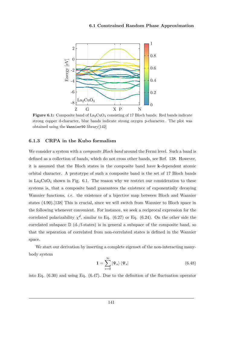
6.1 Constrained Random Phase Approximation
Z G X P N
-8
-6
-4
-2
0
2
La2CuO4
En
ergy
[eV
]
0
0.2
0.4
0.6
0.8
1
Figure 6.1: Composite band of La2CuO4 consisting of 17 Bloch bands. Red bands indicate
strong copper d-character, blue bands indicate strong oxygen p-character. The plot was
obtained using the Wannier90 library[142]
6.1.3 CRPA in the Kubo formalism
We consider a system with a composite Bloch band around the Fermi level. Such a band is
defined as a collection of bands, which do not cross other bands, see Ref. 138. However,
it is assumed that the Bloch states in the composite band have k-dependent atomic
orbital character. A prototype of such a composite band is the set of 17 Bloch bands
in La2CuO4 shown in Fig. 6.1. The reason why we restrict our consideration to these
systems is, that a composite band guarantees the existence of exponentially decaying
Wannier functions, i.e. the existence of a bijective map between Bloch and Wannier
states (4.90).[138] This is crucial, since we will switch from Wannier to Bloch space in
the following whenever convenient. For instance, we seek a reciprocal expression for the
correlated polarizability χd, similar to Eq. (6.27) or Eq. (6.24). On the other side the
correlated subspace D (d-/f-states) is in general a subspace of the composite band, so
that the separation of correlated from non-correlated states is defined in the Wannier
space.
We start our derivation by inserting a complete eigenset of the non-interacting many-
body system
1 =
∞∑s=0
|Ψs〉 〈Ψs| (6.48)
into Eq. (6.30) and using Eq. (6.47). Due to the definition of the fluctuation operator
141

6. MERGING GW WITH DMFT
(6.47) the s = 0 contributions drops out and we obtain
χd(r, r′, τ) = Θ(+τ)∞∑s=1
e(E0−Es)τ 〈Ψ0| nd(r) |Ψs〉 〈Ψs| nd(r′) |Ψ0〉
+ Θ(−τ)
∞∑s=1
e(Es−E0)τ 〈Ψ0| nd(r′) |Ψs〉 〈Ψs| nd(r) |Ψ0〉 . (6.49)
Here we used the Heisenberg relation nd(r, τ) = eH0τ nd(r)e−H0τ and the fact that |Ψs〉is an eigenvector of the non-interacting Hamiltonian H0 of the complete Fock space F,
defined in Eq. (2.2), with corresponding eigenenergy Es.
From Eq. (6.49) the desired expression can obtained in two steps. Both steps are
explained in detail in the following.
Step One: Matrix elements in Wannier Representation
Here the matrix elements 〈Ψ0| nd(r) |Ψs〉 of Eq. (6.49) are evaluated. This is achieved
by using expression (6.45) for the correlated fluctuation operator in combination with
the inverse representation of Eq. (6.39) and yields
〈Ψ0| nd(r) |Ψs〉 =∑αβ∈D
w∗α(r)wβ(r)
∫dr1dr2wα(r1)w∗β(r2) 〈Ψ0| ψ†(r1)ψ(r2) |Ψs〉
(6.50)
Now we focus on the evaluation of the expectation value on the r.h.s. For a Slater
determinant |Ψs〉 the action of the field operator ψ(r2) onto the N electron state
Ψs(r′1, · · · , r′N ) is given by Eq. (2.25), together with the adjoint relation we obtain:
〈Ψ0| ψ†(r1)ψ(r2) |Ψs〉 = N
∫dr′2 · · · dr′NΨ∗0(r1, r
′2, · · · , r′N )Ψs(r2, r
′2, · · · , r′N )
= N[τ∗(0)
]α1α2···αN [τ(s)
]β1
α2···αNw∗α1
(r1)wβ1(r2)
(6.51)
The contraction of the τ tensors in the last line can be evaluated using the identity[47]
[ε(0)
]n1n2···nN [ε(s)
]m1
n2···nN=
(N − 1)!
N !δn1
i(s)δm1
a(s), (6.52)
where i(s) is the occupied state (contained in I0) and is replaced by the unoccupied
state a(s) in the index set Is, and with Eq. (6.34) obtaining[τ∗(0)
]α1α2···αN [τ(s)
]β1
α2···αN=
(N − 1)!
N !T ∗α1
i(s)Tβ1
a(s). (6.53)
142

6.1 Constrained Random Phase Approximation
Therefore, only singly excited Slater determinants |Ψs〉 contribute to the matrix element
(6.50), which may be written as
〈Ψ0| nd(r) |Ψs〉 =∑αβ∈D
w∗α(r)wβ(r)T ∗α1
i(s)Tβ1
a(s) 〈wα1|wα〉︸ ︷︷ ︸
δα
α1
〈wβ∣∣wβ1
⟩︸ ︷︷ ︸δ
ββ1
(6.54)
and results in
〈Ψ0| nd(r) |Ψs〉 =∑αβ∈D
T ∗αi(s)w∗α(r)wβ(r)Tβa(s). (6.55)
Consequently, the Kubo formula (6.49) yields after a Fourier transformation to frequency
domain
χd(r, r′, iν) =∑
αβγδ∈D
∞∑s=1
[Ξ(s)(iν)
]αβγδw∗α(r)wβ(r)w∗γ(r′)wδ(r
′) (6.56)
with the tensor
[Ξ(s)(iν)
]αβγδ=T ∗αi(s)T
βa(s)T
∗γa(s)T
δi(s)
Es − E0 + iν+T ∗αa(s)T
βi(s)T
∗γi(s)T
δa(s)
Es − E0 − iν(6.57)
The sum over singly excited Slater determinants∑
s can be rewritten into a double sum
of Bloch indices i = (n,k),a = (n′,k′) using occupancy functions fi = f(εi) as follows
∞∑s=1
[Ξ(s)(iν)
]αβγδ=
1
N2k
∑nn′kk′
fi(1− fa)
×(T ∗αiT
βaT∗γaT
δi
εa − εi + iν+T ∗αaT
βiT∗γiTδa
εa − εi − iν
)
=1
N2k
∑nn′kk′
fi(1− fa)− fa(1− fi)εa − εi + iν
T ∗αiTβaT∗γaT
δi (6.58)
In the second term on the r.h.s. the indices (i,a) ↔ (a, i) have been swapped. Conse-
quently, Eq. (6.56) can be rewritten into
χd(r, r′, iν) =∑
αβγδ∈D
1
N2k
∑nn′kk′
fi − faεa − εi + iν
T ∗αiTβaT∗γaT
δiw∗α(r)wβ(r)w∗γ(r′)wδ(r
′).
(6.59)
Before continuing with step two, we make two short remarks: Firstly, Eq. (6.59) is the
Wannier representation for the independent particle polarizability (derived by Hanke
143

6. MERGING GW WITH DMFT
and Sham in Refs. 148 and 149), but restricted to the target space D. Secondly, Eq.
(6.59) can be rewritten into1
χd(r, r′, iν) =∑
αβγδ∈D
1
N2k
∑nn′kk′
y(ν, ξai)T∗αiTβaT∗γaT
δiw∗α(r)wβ(r)w∗γ(r′)wδ(r
′),
(6.60)
where i and a are strictly restricted to occupied and unoccupied Bloch indices respec-
tively. Looking at the Bloch representation (6.24), reveals that χd is a contracted four-
point propagator and needs to be transformed to the Bloch domain as a four-point rather
than a two-point tensor. This is done in the next step, where we show that Eq. (6.60)
picks up four additional Wannier transformation matrices Tnα proving that the weighted
expression (6.27) of the target polarizability (containing the diagonal of only four T−matrices) does not follow from the Kubo formula (6.30).
Step Two: Fourier Transformation
In the second step, the Fourier transformation is performed to reciprocal space. The
general prescription for this procedure is described in Ref. 108 and given by:
χdq(g,g′, iν) =
∫dr
∫dr′ei(g+q)rχd(r, r′, iν)e−i(g
′+q)r′ . (6.61)
Decomposing the Wannier functions into Bloch functions and using n1 = (n1,k1) as in
Eq. (6.37) we obtain
χdq(g,g′, iν) =1
N2k
∑nn′kk′
1
N4k
∑n1n2n3n4
∑αβγδ∈D
y(ν, ξia)
T ∗(k)αn T (k1)
αn1〈φn1 | ei(g+q)r |φn2〉T
∗(k2)βn2
T(k′)βm
T ∗(k′)
γm T (k3)γn3〈φn3 | e−i(g
′+q)r′ |φn4〉T∗(k4)δn4
T(k)δn∑
Rα
eiRα(k1−k)∑Rβ
e−iRβ(k2−k′)∑Rγ
eiRγ(k3−k′)∑Rδ
e−iRδ(k4−k)
(6.62)
1 To see this, first one decomposes the factor (ξai+ iν)−1 into a symmetric and antisymmetric tensor
in a, i. That is1
ξai + iν=
ξaiξ2ai + ν2︸ ︷︷ ︸
12y(ν,ξai)
−i ν
ξ2ai + ν2
.
In the next step, one uses the fact that both, the factor (fi − fa) as well as the first term on the r.h.s.
are odd tensors in i,a and therefore are non-zero, whereas the second term is an even tensor in i,a and
vanishes.
144

6.1 Constrained Random Phase Approximation
The sum over lattice vectors R can be carried out using the simple identity[108]∑R
eikR =∑g
δkg. (6.63)
and restricts the k-vectors
k1 = k + g1, k2 = k′ + g2, k3 = k′ + g3, k4 = k + g4, (6.64)
where g1 · · ·g4 are reciprocal lattice vectors. Furthermore, the periodicity condition[139]
T (k)nα = T (k+g)
nα (6.65)
allows to carry out the sum over lattice sites α · · · δ resulting in four projectors defined
in Eq. (6.31). Hence, the sum over reciprocal lattice vectors g1, · · · ,g4 yields four times
the same contribution, namely
χdq(g,g′, iν) =1
N2k
∑nn′kk′
y(ν, ξai)⟨φi∣∣ ei(g+q)r
∣∣φa⟩ ⟨φa∣∣ e−i(g′+q)r′∣∣φi⟩ , (6.66)
where the definition of the correlated Bloch functions (6.32) have been used with the
short hands i = (n,k) and a = (n′,k′). Pointing out, that the matrix elements on the
r.h.s. of Eq. (6.66) are invariant under the transformations r→ r + R and r′ → r′ −R
reveals the restriction on the primed k-point
k′ = k + q. (6.67)
This removes an additional factor N−1k and we obtain the main result of this section
χdq(g,g′, iν) =1
Nk
∑nn′k
y(ν, ξai)⟨φi∣∣ ei(g+q)r
∣∣φa⟩ ⟨φa∣∣ e−i(g′+q)r′∣∣φi⟩ , (6.68)
with i = (n,k) representing the occupied and a = (n′,k + q) the unoccupied indices.
If the composite band consists only of target states, i.e. the target space D forms an
isolated set of Bloch bands, the projectors (6.31) become diagonal and expression (6.68)
reduces to the constrained Adler and Wiser form (6.24). The weighted expression of
Sasıoglu et al. (respectively and Shih and coworkers) Eq. (6.27) follows only from the
replacement ∣∣φnk⟩→√P
(k)nn |φnk〉 (6.69)
in Eq. (6.68), which seems, to be an unjustifiable ad-hoc step.
145

6. MERGING GW WITH DMFT
6.1.3.1 Technical details
In this section we discuss technical details of our CRPA implementation. The derivation
of Eq. (6.68) holds strictly for an isolated set of Bloch bands (composite Bloch band)
that can be represented by the localized Wannier functions
|wαk〉 =∑n
T (k)αn |φnk〉 . (6.70)
For systems, where such a set of bands is absent (for instance the 3d transition metals
series Sc-Ni), expression (6.68) is not uniquely defined. From the practical point of view,
this is due to the ill-conditioned ”inverse projection” of Eq. (4.90). However, we found
that one can use the regularized projectors
P (k)nm = Θ(k)
m P (k)nm (6.71)
instead. Here the window function Θ(k)m is either 0 (for a null-vector) or 1 (for a rank-
vector) and is obtained from the Jacobi diagonalization of the original projector P(k)nm .[92,
150]
To illustrate this regularization procedure, we consider the case where Bloch bands
are projected onto Wannier states via the projector
T (k)nα =
,
with and indicating a non-zero and zero entry respectively. In this specific example
the Bloch bands φ2, · · · , φ5 are projected onto the Wannier states w1, w2 and w3. The
corresponding correlated projector P(k)nm assumes the form
P (k)nm =
146

6.1 Constrained Random Phase Approximation
and the resulting (N − ND) × (N − ND) non-zero sub-block (here N − ND = 4) has
rank ND. For instance, if the Jacobi diagonalization of P(k)nm yields diag(1, 1, 0, 1) for this
sub-block, the regularized projector P(k)nm is
P (k)nm = Θ(k)
m P (k)nm =
and has ultimately the same number of rows and columns as T
(k)nm .
Once the correlated polarizability (6.68) is determined, we subtract it from the full
polarizability (3.41), yielding the effective polarizability χr. In the next step the screen-
ing equation (6.21) is solved for the effective kernel Ugg′(q, iν) for every k-point q in
the irreducible wedge of the Brillouin zone. In the final step the interaction matrix is
evaluated via
Uαβγδ =1
N2k
∑qk
∑gg′
Ugg′(q, 0) 〈wαk| ei(q+g)r |wδk+q〉 〈wβk+q| e−i(q+g′)r′ |wγk〉 , (6.72)
with the mixed basis representations (6.70).
We emphasize that our approach, i.e. the correlated polarizability (6.68) and effec-
tively the matrix elements (6.72), differ from the disentanglement method of Miyake and
coworkers, since in contrast to Ref. 145 we do not change the original band structure.
6.1.4 Computational details
We have considered the high temperature superconductor La2CuO4 and the 3d transition
metal series Sc up to Ni. The lattice constants for the latter are obtained by minimizing
the PBE density functional[106] and are summarized in Tab. 6.1. For the cuprate the
lattice constant a = 3.86 A and a ratio of c/a = 3.41 for the bct unit cell was used
with the positions given in Tab. 6.2. Convergence of the effective interaction matrix
(6.72) w.r.t. the plane wave basis set is reached using the same method as described
in Ref. 151. First, the effective matrix elements (6.72) are determined using a rather
low energy cutoff Ecut for the CRPA polarizability χr on a plane wave grid. This result
is corrected by the difference of the bare Coulomb interaction Vαβγδ obtained with the
147

6. MERGING GW WITH DMFT
Table 6.1: Used structures for the transition metal (TM) series. Lattice constants are
given in A and obtained from PBE.
Sc Ti V Cr Mn Fe Co Ni
fcc fcc bcc bcc bcc bcc fcc fcc
4.64 4.13 2.99 2.85 2.78 2.77 3.47 3.52
Table 6.2: Atomic positions in La2CuO4 in direct coordinates
Atom Position
x y z
La 0.64 0.64 0.00
La 0.36 0.36 0.00
Cu 0.00 0.00 0.00
O 0.00 0.50 0.50
O 0.50 0.00 0.50
O 0.19 0.19 0.00
O 0.81 0.81 0.00
148

6.1 Constrained Random Phase Approximation
same cutoff on the same grid and Vαβγδ obtained using the exact all-electron method
described in Ref. 96 with a higher cutoff Ecut. This is justified, since the high energy
contributions to the polarizability χr vanish and the screening becomes ineffective for
large g vectors.[151]
In all calculations we included 128 bands and plane wave contributions up to a cutoff
of Ecut = 400 eV in the calculation of the CRPA polarizability. For the high cutoff Ecut
700 eV and for the PAW basis set a cutoff of 500 eV was chosen. In order to obtain
a well-converged groundstate, a dense k-point grid of 16 × 16 × 16 points was used in
combination with the tetrahedron method of Blochl et al.[152] with a smearing factor of
σ = 0.2 eV−1.
6.1.5 Wannier basis
The quality of the Wannier basis is a crucial point for all CRPA methods. Therefore,
we discuss here in detail, how the localized basis is obtained.
We start with the superconductor La2CuO4, which possesses an isolated composite
band of 17 Bloch bands. These states correspond to the 12 p-states centered at the four
oxygen atoms and the five d-states centered at the copper atom in the unit cell. We,
therefore, transform these bands to 17 Wannier states and call this the dp basis in the
following. The quality of the Wannier transformation is investigated by diagonalizing
the corresponding Wannier Hamiltonian and comparing with the original PBE band
structure. The comparison is given in Fig. 6.1 and shows that the match is perfect
already at a rather coarse k-point mesh of 8 × 8 × 8 points. We have used this k-point
setting for both, the Wannier transformation as well as the CRPA calculations.
In contrast to the cuprate, the 3d transition metals do not possess an isolated set
of bands. However, a one to one correspondence between six Wannier states and six
bands around the Fermi level, five narrow bands (mainly of d-character) and a crossing
s-like band, can be achieved. Thereby the location of the s-state was chosen at the
reciprocal coordinates (0.25, 0.25, 0.25) for the fcc and at (0.5, 0.5, 0.5) for the bcc unit
cells, whereas the d-states are centered at the TM. We call this basis set the ds basis in
the following and show in Fig. 6.2 (a) a comparison between the original PBE bands
of Ni and the eigenvalues of the Hamiltonian in the ds basis. One clearly sees that
the ds basis reproduces most symmetry lines accurately, but has difficulties to represent
the symmetry points W and K of the s-state. This is due to the fact, that these
149

6. MERGING GW WITH DMFT
G X W L G K
-8
-6
-4
-2
0
2
4
6
8
(a)
En
ergy
[eV
]
0
0.2
0.4
0.6
0.8
1
-8
-6
-4
-2
0
2
4
6
8
G X W L G K
En
ergy
[eV
]
(b)
Figure 6.2: Bands of fcc Ni with d-character resolution obtained from Wannier90. Red
bands indicate strong d-character, blue bands indicate strong s-character. (a) d-character
resolution in ds basis. (b) Comparison of disentangled system (red and blue bands) with
original system (gray bands) in d basis.
Table 6.3: Used energy windows in [eV] for the construction of the d basis in the 3d series.
The Fermi level is set to 0 eV.
Sc Ti V Cr Mn Fe Co Ni
Emin −3.0 −4.0 −4.5 −4.5 −6.0 −6.0 −6.5 −7.5
Emax +5.0 +5.0 +5.5 +5.5 +5.0 +5.0 +4.0 +3.5
points are crossing points with higher energy states and since the Wannier basis is
lacking this information, the eigenvalues of the Wannier Hamiltonian start to oscillate.
Consequently, the representability of the ds basis is never perfect, as it is in the case of
the aforementioned dp basis for La2CuO4. To compensate this defect, we have decided
to use a very dense 16× 16× 16 k-point grid for the Wannier projection.
In addition to the ds basis, we considered a third basis set. The d basis contains
only five d-states and is obtained as a projection of the same six Bloch bands using the
energy windows given in Tab. 6.3 for the method of Souza.[143] For Ni we show in Fig.
6.2 (b) the eigenvalues of the Hamiltonian in this basis (red bands). The same figure
shows, in addition, the original PBE bands and the disentangled s-band (blue band),
which was obtained by applying the method of Miyake et al.[147]
Last but not least, we have compared the spatial spread of the two basis sets, given
in Fig.6.3. It can be seen that the inclusion of the s-state tends to yield more localized
150

6.1 Constrained Random Phase Approximation
0
0.5
1
1.5
2
2.5
3
Sc Ti V Cr Mn Fe Co Ni
Sp
read
[A2]
d†ds
Figure 6.3: Average spread of Wannier d-functions of the TM series in the d (squares) and
ds (points) basis. For comparison data of Ref. 153 (†) is given for the d basis.
(delocalized) Wannier functions in the fcc (bcc) unit cells. The general decreasing spread
towards the right in the series is evident and expected.
6.1.6 Transition metals
In the following subsection, we discuss our results for the bare V , fully screened W
and effective interaction averages U , defined in Eqs. (6.17), (6.18) and (6.14) for the
transition metal series Sc-Ni. For the CRPA calculations we have considered three
distinct models, summarized in Tab. 6.4. Model (i) corresponds to the disentanglement
method of Ref. 147, model (ii) is the the weighting method in the ds basis of Refs. 145
and 146, whereas model (iii) is the CRPA approach derived in section 6.1.3.
Table 6.4: Used models.
model basis applied to χd
(i) d TMs Eq.(6.24)
(ii) ds/dp TMs/La2CuO4 Eq.(6.27)
(iii) ds/dp TMs/La2CuO4 Eq.(6.68)
6.1.6.1 Bare Coulomb interaction
As a starting point of our investigation we have evaluated the bare Hubbard-Kanamori
interaction V for both basis sets d and ds. For the latter we have averaged only over the
d-states of the TMs. The results in the d basis are shown in Fig. 6.4 (a) (red points)
151

6. MERGING GW WITH DMFT
together with published values. We see good agreement with Shih et al.1 and for the
early transition metals Sc, Ti, and V with an increasing discrepancy for the later TMs,
reaching the largest difference of 2.76 eV for Ni. This can be related to the second
energy window used in Ref. 154 yielding ultimately a different basis than in the present
work. If the same Wannier settings are chosen (compare to Ref. 153) one obtains almost
identical interactions.
10
15
20
25
30
Sc Ti V Cr Mn Fe Co Ni
(a)
]†present
10
15
20
25
30
Sc Ti V Cr Mn Fe Co Ni
(b)
]‡§present
Figure 6.4: Bare Coulomb repulsion V in [eV] of 3d TMs series in d (a) and ds basis (b).
For comparison Ref.]146, Ref.†153, Ref.§145 and Ref.‡155 are given
The inclusion of the s-state in the localized basis set (basis ds) tends to yield more
localized d-states in the fcc unit cells. The consequence is that the bare interaction in
the ds basis is larger than in the d basis, as can be seen in Fig. 6.4 (b), for Sc, Ti, Co and
Ni. Despite the fact, that the spread of the d-states in the ds basis is slightly larger (see
Fig. 6.3), the bare interaction is still slightly larger in the ds basis than in the minimal
basis set. For instance the difference to the d basis for bcc Cr is around 1.7 eV. Hence,
we conclude that the presence of the additional s-state compensates the larger spread
in the ds basis. Compared to literature, we obtain excellent agreement with Sasıoglu et
al.[145, 155] and Shih et al.[154].
6.1.6.2 Fully screened RPA interaction
Next, we investigated the fully screened interaction W on the random phase approxima-
tion level in both basis sets d and ds. In contrast to the ds basis, the minimal d basis
allows for two different calculations.[147] On the one side, the original PBE eigensystem
[gray bands in Fig. 6.2 (b)] can be used for the determination of the RPA polarizability
1See Ref. 146 and references therein.
152

6.1 Constrained Random Phase Approximation
0
0.5
1
1.5
2
2.5
3
Sc Ti V Cr Mn Fe Co Ni
(a)
dis♦
orig♦
disorig
0
0.5
1
1.5
2
2.5
3
Sc Ti V Cr Mn Fe Co Ni
(b)
§‡present
Figure 6.5: (a) On-site fully screened d-Coulomb repulsion measured in [eV] in d basis of
disentangled (squares) and original Kohn-Sham system (circles). (b) Full RPA interaction
of original system in ds basis. For comparison Ref.♦ 147, Ref.§ 145 and Ref.‡ 155 are shown.
in Eq. (6.19). On the other side, the latter can be computed using the disentangled
system [blue and red bands in 6.2 (b)]. In both cases the resulting interaction kernel
WGG′(q, ω) is evaluated in the d basis [red bands in Fig. 6.2 (b)].
The results for the TMs with the original Kohn-Sham system are given by the red
points in Fig. 6.5 (a), whereas the filled squares show W obtained from disentanglement.
Comparing the latter with the red points in Fig. 6.5 (a) shows that the disentanglement
effect can be safely disregarded. The same figure shows, in addition, previously published
data of Ref. 147 (circles and empty squares). All in all, the agreement is good, except
for Mn and Fe, where we obtain considerably larger interactions. Most probably, as
discussed below, this can be related to the pseudo potentials, even tough we used slightly
different energy windows in our calculations (see previous section).
The fully screened interaction in the ds basis is shown in Fig. 6.5 (b) (filled circles).
Comparing to the minimal d basis, the interactions are again slightly larger due to the
stronger localization of the d-states [compare dots in Fig. 6.5 (a) and (b)]. The same
figure shows in addition published data of Sasıoglu et al. in 2011 (empty squares) and
2013 (empty circles) respectively.[145, 155] Here we observe excellent agreement for early
metals up to bcc Cr with small deviations starting at bcc Mn and increasing towards
Ni. We mainly make the used pseudo potentials responsible for the discrepancies to the
literature.
153
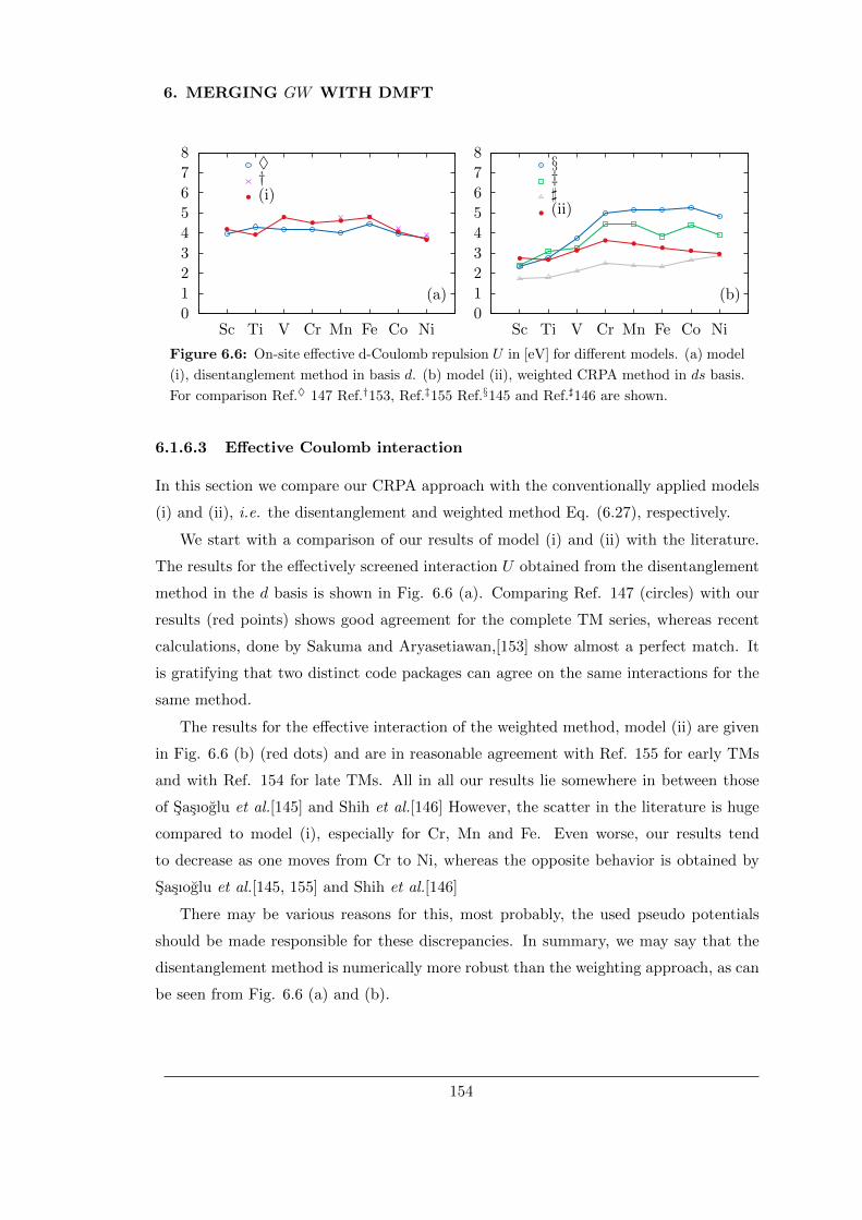
6. MERGING GW WITH DMFT
0
1
2
3
4
5
6
7
8
Sc Ti V Cr Mn Fe Co Ni
(a)
♦†(i)
0
1
2
3
4
5
6
7
8
Sc Ti V Cr Mn Fe Co Ni
(b)
§‡](ii)
Figure 6.6: On-site effective d-Coulomb repulsion U in [eV] for different models. (a) model
(i), disentanglement method in basis d. (b) model (ii), weighted CRPA method in ds basis.
For comparison Ref.♦ 147 Ref.†153, Ref.‡155 Ref.§145 and Ref.]146 are shown.
6.1.6.3 Effective Coulomb interaction
In this section we compare our CRPA approach with the conventionally applied models
(i) and (ii), i.e. the disentanglement and weighted method Eq. (6.27), respectively.
We start with a comparison of our results of model (i) and (ii) with the literature.
The results for the effectively screened interaction U obtained from the disentanglement
method in the d basis is shown in Fig. 6.6 (a). Comparing Ref. 147 (circles) with our
results (red points) shows good agreement for the complete TM series, whereas recent
calculations, done by Sakuma and Aryasetiawan,[153] show almost a perfect match. It
is gratifying that two distinct code packages can agree on the same interactions for the
same method.
The results for the effective interaction of the weighted method, model (ii) are given
in Fig. 6.6 (b) (red dots) and are in reasonable agreement with Ref. 155 for early TMs
and with Ref. 154 for late TMs. All in all our results lie somewhere in between those
of Sasıoglu et al.[145] and Shih et al.[146] However, the scatter in the literature is huge
compared to model (i), especially for Cr, Mn and Fe. Even worse, our results tend
to decrease as one moves from Cr to Ni, whereas the opposite behavior is obtained by
Sasıoglu et al.[145, 155] and Shih et al.[146]
There may be various reasons for this, most probably, the used pseudo potentials
should be made responsible for these discrepancies. In summary, we may say that the
disentanglement method is numerically more robust than the weighting approach, as can
be seen from Fig. 6.6 (a) and (b).
154

6.1 Constrained Random Phase Approximation
0
1
2
3
4
5
6
7
8
Sc Ti V Cr Mn Fe Co Ni
U[e
V]
(i)(ii)(iii)
Figure 6.7: Comparison of present CRPA approach, model (iii) (red points), with disen-
tangling (i) and weighted method (ii).
We complete this subsection with the discussion of results obtained with our ap-
proach, i.e. model (iii). A comparison with model (i) and (ii) is given in Fig. 6.7. First,
we observe that the overall trend of model (ii) (squares) and (iii) (points) is similar and
differs from model (i) (circles). This might be related to the disentanglement used in
model (i). Second, comparing model (ii) with (iii) one sees that our approach yields in
general larger interactions than (ii). This comes from the fact, that Eq. (6.68) removes
more screening effects than the weighted formula (6.27), since also off-diagonal terms of
the projectors (6.31) are taken into account in the correlated polarizability. The result-
ing effective polarizability is smaller, the corresponding screening is less effective and
shifts the effective interaction U of model (iii) towards the values of model (i). However,
the shift is not constant and varies from system to system. In general, we observe a
smaller shift for the fcc than for the bcc structures.
Last but not least we have investigated the low frequency dependence of model (i)-
(iii) for fcc Ni and bcc Cr. The frequency regime shown in Fig. 6.8 might be of interest
for frequency dependent DMFT calculations. The solid red line represents model (iii),
the dashed green curve model (ii) and the dashed blue curve stands for model (i). One
observes a rather flat low frequency behavior for model (i) in Ni and Cr. However,
model (ii) and (iii) show more structure. Whereas the difference between the weighted
and our CRPA approach is negligible for fcc Ni, the difference in bcc Cr is clearly visible
around 3 eV and approaches the analytically continued data of Sasıoglu et al. for higher
frequencies. This implies that the conventionally chosen static approximation (6.12) of
the CRPA might be problematic and needs to be further investigated.
155

6. MERGING GW WITH DMFT
0
2
4
6
8
10
12
14
0 2 4 6 8 10Frequency [eV]
Cr
0 2 4 6 8 100
2
4
6
8
10
12
Frequency [eV]
Ni
(i)(ii)(iii)
(i)(ii)
(iii)
Figure 6.8: Frequency dependence of effectively screened interaction for fcc Ni and bcc
Cr in model (i) (blue), model (ii) (green) and model (iii) (solid line). The gray line shows
analytically continued data of model (ii) published in Ref. 155.
6.1.7 La2CuO4
La2CuO4 is the prototype of a high temperature superconductor and has been heavily
studied in the condensed-matter community since the 1980s. In the following, we want
to sketch only the most important aspects of this compound, which are necessary for the
computation of the effective interaction in the one-band and five-band Hubbard model.
The interested reader is referred to literature.[156, 157, 158, 159]
PBE yields the band structure given in Fig. 6.1. The single band crossing the Fermi
surface makes this compound interesting for single-band DMFT studies. This band is
often referred to as the dx2−y2 state of Cu, however, Fig. 6.1 shows that it is strongly
entangled with the surrounding oxygen p-states. Therefore the dp basis mentioned in
section 6.1.5 is a good choice to study the interactions of this compound.
As for the TM series, we first determined the bare and fully screened interactions
V and W . The complete interaction matrices Vααββ , Vαβαβ ,Wααββ and Wαβαβ of the
d-submanifold are given in the appendix E. It can be seen that the dx2−y2-dx2−y2 matrix
element has the largest value, 28.7 eV for the bare and 2.6 eV for the fully screened
interaction.
Next we have considered the effective interaction of the one-band model. Here only
the intra dx2−y2-dx2−y2 screening effects are removed. Using the CRPA method devel-
oped in this paper we obtain an effective interaction of U = 3.0. This is only 0.1 eV larger
156

6.1 Constrained Random Phase Approximation
than in the weighting approach of model (ii) and both models are in reasonable agree-
ment with the chosen U in recent one-band DMFT studies of this compound.[160, 161]
If, however, the complete d-manifold is considered as target space in the CRPA
the difference between the weighting and our model becomes evident. For model (ii) we
obtain an averaged interaction of U = 3.7, whereas model (iii) yields U = 5.7 eV. Recent
multi-orbital LDA+DMFT calculations used interaction parameters between 4 and 10
eV.[162] The complete Hubbard matrices Uααββ and Uαβαβ of model (iii) are given in
Tab. 6.5.
Table 6.5: Effective Hubbard interaction matrices Uααββ and Uαβαβ for La2CuO4 obtained
with model (iii).
dxy dxz dyz dx2−y2 dz2 dxy dxz dyz dx2−y2 dz2
dxy 5.8 4.4 4.4 3.5 3.5 5.4 0.7 0.7 1.1 1.1
dzy 4.4 5.7 3.9 3.7 3.7 0.7 5.3 0.9 1.0 0.9
dyz 4.4 3.9 5.7 3.7 3.7 0.7 0.9 5.3 1.0 0.9
dx2−y2 3.5 3.7 3.7 5.6 4.4 1.1 1.0 1.0 5.2 0.6
dz2 3.5 3.7 3.7 4.4 5.5 1.1 0.9 0.9 0.6 5.1
157

6. MERGING GW WITH DMFT
6.2 Unscreening Method for Isolated Target States
Large parts of the following section have been published in Ref. 151.
In this section we consider the special case, where the correlated subspace D is
restricted to the target states located the impurity cell R = 0. This means that only
local excitations are neglected in the RPA screening process. We shall see in moment
that this approach is applicable only for isolated target bands, where a minimal Wannier
basis can be found. The method relies on the general recipe given already in Eq. (6.2)
and requires the knowledge of both, the on-site fully screened interaction Wαβγδ as well
as the independent particle polarizability χ0αβγδ in the Wannier basis at R = 0. One
can say that the effective matrix elements Uαβγδ are obtained from unscreening the fully
screened interaction using the impurity polarization.
Eq. (6.2) can be rewritten into the common Dyson form
Wαβγδ = Uαβγδ + Uαρτδχ0ρµντW
µβγν . (6.73)
In the previous sections we have determined the on-site fully screened interaction matrix
Wαβγδ. What remains, to solve the equation above for the matrix elements Uαβγδ, is to
determine the correlated polarizability tensor χ0αβγδ. Fortunately, this follows trivially
from Hanke’s expression, derived in (6.59), by renaming δ → γ, β → δ, γ → β and
restricting the lattice vectors Rα −Rδ to the impurity cell R = 0. One then obtains
χαβγδ0 (iν) =1
N2k
∑ia
y(ν, ξai)T∗αiT
βaT∗γaT
δi, (6.74)
with i = (nk) denoting the occupied and a = (n′k + q) the unoccupied Bloch index.
We introduce the composite indices (α, δ), (β, γ), (ρ, τ), (µ, ν) to represent the cor-
responding matrix elements in Eq. (6.73) by conventional matrices U ,χ0,W . This
allows us to rewrite the equation into the computationally convenient matrix form
U = W · (1 + χ0 ·W )−1. (6.75)
However, a closer look to Eq. (6.73) reveals a problem if the target space is smaller
than the space spanned by the Wannier states, like for instance for the systems investi-
gated in the previous section. In this case the correct unscreening equation is
Wαβγδ = Uαβγδ +∑
ρµντ∈DUαρτδχ0
ρµντWµβγν (6.76)
158
6.2 Unscreening Method for Isolated Target States
and is ill-defined, because the corresponding matrix equation (6.75) contains matrices of
different dimensions, see Ref. 163 for a similar discussion. To our knowledge there is no
unambiguous regularization scheme for such equations, so that the unscreening method
described above is ultimately restricted to a small class of materials. One example for
such a system is SrVO3 and is discussed in section 6.2.2.
6.2.1 Implementation Details
We have implemented this method into VASP using the same technique as in section
section 6.1.3.1, with one noteworthy difference. We impose an energy cutoff of 1000 eV−1
on the polarizability tensor χ0 to be consistent with metallic screening, Wq→0(0,0, 0)→0. We found that this approach improves remarkably the stability of the unscreening
method.
6.2.2 Application to SrVO3
We have compared the unscreening method with the CRPA approach, derived in section
(6.1.3) for the test bet material SrVO3. This material is a d1 metal and one of the
most benchmarked systems within LDA+DMFT.[83] We have considered the the ideal
perovskite structure, shown in Fig. 6.9 with a lattice constant of a = 3.78 A. The
perovskite is characterized by Sr atoms located between octahedral crystal fields (red
octahedra) build by six oxygen atoms with a V atom (not visible) in the center. The
octahedral crystal field splits the five-fold energetically degenerate atomic d-states of V
into two subgroups, the t2g- and eg-states consisting of three, respectively two states
with same energy. More precisely, the eg-group contains the dz2- and dx2−y2-states and
lies higher in energy than the t2g-group consisting of the dxy-, dxz- and dyz-state. This
becomes evident by considering the band structure of the system shown in Fig. 6.9,
where the two blue bands above Fermi level (at µ = 0 eV) are mainly of eg character
and the the three bands crossing the Fermi surface are the t2g-states.
These properties have two advantages. First, considering the t2g-states as target
space for DMFT is computationally convenient, due to the presence of only three cor-
related states. Second, the t2g manifold is topologically separated from the remaining
Fock space and forms a composite Bloch band.[138] We, therefore, are able to compare
the unscreening method, presented above, with the CRPA approach of section 6.1.3.
159

6. MERGING GW WITH DMFT
-6
-4
-2
0
2
4
6
R Γ X M Γ
[eV
]Figure 6.9: Left: Crystal structure of SrVO3. Sr atoms (green) are located between the
oxygen crystal fields indicated by red octahedra with a V atom in the center. Right: Band
structure of SrVO3. The three t2g-states of V cross the chemical potential chosen at µ = 0
eV.
6.2.3 Comparison with CRPA
We have chosen maximally localized Wannier states as basis for our calculations. [140]
These states were obtained from the Wannier90 library by excluding all, except the
three t2g-bands of V, in the projection.[142] The plane wave cutoff energies for the
orbitals and the CRPA-polarizability have been set to 414 eV and 350 eV respectively.
Extrapolation to a high energy cutoff of 500 eV was performed as described in section
6.1.4 and a Methfessel-Paxton smearing function was chosen for the Fermi occupancies
with σ = 0.1.[164]
Due to the ideal perovskite structure any interaction matrix of SrVO3, including
the effective matrix Uαβγδ are determined by the three Hubbard-Kanamori parameters
(6.14)-(6.16). They are given in Tab. 6.6 for the unscreening U and the CRPA method,
denoted by UCRPA. The same table shows, in addition, the Hubbard-Kanamori parame-
ter for the bare Coulomb and fully screened interaction. The bare Coulomb interactions
(∼ 16 eV) are largely screened by the high-energy bands to give UCRPA ∼ 3 eV. In the
present case of SrVO3, the unscreened U turns out to have a value similar to UCRPA.
It can be shown that the unscreened U and U ′ depend strongly on the filling of the
system, which is mainly due to an oscillatory antiscreening effect induced by non-local
160

6.2 Unscreening Method for Isolated Target States
Table 6.6: On-site bare (V ), fully screened RPA (W ), constrained RPA UCRPA and
unscreening interaction (U).
V W UCRPA U
U 16.0 1.12 3.36 3.46
U ′ 14.8 0.30 2.35 2.47
J 0.55 0.39 0.49 0.47
polarizations. This effect is absent in the CRPA method, because here on-, as well as
off-center terms are removed completely in screening and consequently the screening
oscillations are ’flatten out’. The small difference of 0.1 eV between U and UCRPA is
just a consequence of an accidental cancellation of the antiscreening by the non-local
polarizations with the screening by the long-range interaction. More details about this
effect can be found in Ref. 151.
However, we found that apart form the limited applicability of the unscreening
method, the additional antiscreening effect can cause serious issues for other systems.
This effect is not present for the method presented in previous section and it seems
that CRPA is much more reliable than the unscreening scheme. We, therefore, suggest
to apply the CRPA approach whenever possible to determine effective interactions for
model Hamiltonians.
161

6. MERGING GW WITH DMFT
6.3 Quasi Particle GW+DMFT
In this section we apply the qpGW+DMFT algorithm to the test bed material SrVO3.
In addition, a comparison with conventional LDA+DMFT calculations are given.
The following subsection were published in Ref. 165.
6.3.1 Comparing qpGW+DMFT and LDA+DMFT for SrVO3
The starting point of our calculation is the GW implementation within VASP. Specifically,
we first performed Kohn-Sham density functional theory calculations within the settings
mentioned in section 6.2.2 to obtain one-electron orbitals φnk and one-electron energies
εnk. The position of the GW quasi particle peaks εnk were calculated by solving the
linearized Eq. (4.65) for the diagonal
εnk = εnk + ZnkRe[〈φnk| T + ϕ+ Vh + Σ(k, εnk) |φnk〉 − εnk
], (6.77)
where Σ is the G0W0 self-energy and Znk the renormalization factor
Znk =1
1− Re 〈φnk| ∂Σ(k,ω∂ω
∣∣∣ω=εnk
|φnk〉. (6.78)
The original Kohn-Sham orbitals are maintained at this step and expressed in the pro-
jector augmented wave basis. Using Wannier90 these orbitals are projected onto the
minimal t2g Wannier basis, presented in section 6.2.2. To construct an effective low-
energy Hamiltonian for the vanadium t2g orbitals, we follow Faleev, van Schilfgaarde,
and Kotani and approximate the frequency dependent G0W0 self-energy by an hermitian
operator
Σnm,k =1
2〈φnk| Σ†(εnk) + Σ(εnk) |φmk〉 . (6.79)
This qp approximation is commonly used in GW calculations, in particular for self-
consistent calculations, since fully frequency dependent calculations are computationally
very demanding, see section 4.2.1 for more details.
In practice, for the present calculations, we have applied the slightly more involved
procedure to derive an hermitian approximation outlined in Ref. 65, although this yields
essentially an almost identical hermitian operator Σnmk. Furthermore, the off-diagonal
components are found to be negligibly small, and henceforth disregarded. The final
hermitian and k-point dependent operator is transformed to the Wannier basis and
162

6.3 Quasi Particle GW+DMFT
passed on to the DMFT code, where it is used to construct the k-dependent self-energy
by adding the local DMFT self-energy.
This qpGW+DMFT procedure allows us to maintain the structure and outline of the
common DFT+DMFT scheme and can be easily adopted in any DMFT code. Instead
of the LDA one-electron matrix elements, the qpGW ones are passed to the DMFT.
This procedure neglects lifetime broadening and any frequency dependence of the GW
self-energy beyond its linear part. Subtracting the local part of this qpGW hermitian
operator (to avoid a double counting) does not yield a constant shift for the degenerate
t2g orbitals, see for instance Tomczak et al.[166]. However, due to an implementation
error, the calculations have been performed, such that the removal of the local self-energy
terms results in a constant shift of the G0W0 energies. Our approach is, therefore, similar
to LDA+DMFT, but with renormalized band structure. Let us also note that hitherto
we did not perform self-consistency on the GW part.
-8
-6
-4
-2
0
2
4
R Γ X M Γ-2
-1.5
-1
-0.5
0
0.5
1
1.5
2
2.5
R Γ X M Γ
Figure 6.10: (Color online) Left panel: G0W0 quasi particle bands (red) in comparison to
LDA (gray). The Fermi level sets our zero of energy and is marked as a line. Right panel:
Wannier projected t2g band structure from G0W0 (red) and LDA (gray). The t2g target
bands bandwidth is reduced by ∼ 0.7 eV in GW .
Figure 6.10 shows the obtained G0W0 band structure, which for the t2g vanadium
target bands is about 0.7 eV narrower than for the LDA. The oxygen p band (below −2
eV) is shifted downwards by 0.5 eV compared to the LDA, whereas the vanadium eg
bands (located about 1.5 eV above the Fermi level) are slightly shifted upwards by 0.2
eV. In the LDA, the top most vanadium t2g band at the M point is slightly above the
163

6. MERGING GW WITH DMFT
lowest eg band at the Γ point, whereas the G0W0 correction opens a gap between the
t2g and eg states.
Within this Wannier basis, we use an interaction value of Unl = 3.4 eV, as obtained
from the unscreening method described in section 6.2. It can be expected, that the
CRPA interaction of UCRPA = 3.3 eV will yield similar results, however, this might not
be the case for other materials and doping levels. We carefully compare qpGW+DMFT
with LDA+DMFT calculations and experiment. In both cases, we use (frequency-
independent) interaction. The Kanamori interaction parameters as derived from the
locally unscreened RPA are listed in Tab. 6.6 and are almost identical to the CRPA. In
constrained LDA (CLDA), on the other hand, somewhat larger interaction parameters
were obtained and are employed by us for the corresponding calculations UCLDA = 5.05
eV, U ′CLDA = 3.55 eV and JCLDA = 0.75 eV.1[167]
For the subsequent DMFT calculation we employ the Wurzburg-Wien w2dynamics
code,[168] based on the hybridization-expansion variant [169] of the continuous-time
quantum Monte Carlo (CT-QMC) method.[170] This algorithm is particularly fast since
it employs additional quantum numbers for a rotationally invariant Kanamori interaction.[171]
The maximum entropy method is employed for the analytic continuation of the imagi-
nary time and (Matsubara) frequency CT-QMC data to real frequencies, see Ref. 172
for more details.
All our calculations are without self-consistency, which is to some extent justi-
fied for SrVO3. Since the three t2g bands of SrVO3 are degenerate, DMFT does not
change the charge density of the low-energy t2g manifold and hence self-consistency
effects are expected to be small for LDA+DMFT. This is, in principle, different for
qpGW+DMFT. Here the frequency dependence of the DMFT self-energy might yield
some feedback already for a simplified Faleev, van Schilfgaarde and Kotani quasi par-
ticle self-consistency.[173, 174] Finally, we also test the ZB-factor renormalized GW
bandwidth with ZB = 0.7 obtained in Ref. 175 for mimicking the frequency dependence
of the CRPA interaction.
1Note that CLDA tends to overestimate the Hund’s exchange, see Ref. 83 so that in subsequent
LDA+DMFT calculations smaller values of have been employed. For the system SrVO3 this smaller
value of mainly influences the upper Hubbard band.
164

6.3 Quasi Particle GW+DMFT
6.3.2 Results
For analyzing the differences between qpGW+DMFT and LDA+DMFT we analyze and
compare five different calculations in the following:
(1) LDA+DMFT@U′cLDA(conventional LDA+DMFT calculation with the CLDA in-
teraction U′CLDA = 3.55 eV).
(2) LDA+DMFT@U′nl(LDA+DMFT calculation but with the locally unscreened RPA
interaction U′nl = 2.49 eV).
(3) qpGW+DMFT@U′nl(qpGW+DMFT calculation with U
′nl = 2.49 eV).
(4) qpGW+DMFT@U′cLDA(qpGW+DMFT calculation with U
′CLDA = 3.55 eV).
(5) qpGW+DMFT@U′nl,ZB = 0.7 (as 3 but with a Bose renormalization factor ZB).
Let us first turn to the imaginary part of the local self-energy which is shown as
a function of (Matsubara) frequency in Fig. 6.11. The self-energy yields a first im-
pression of how strong the electronic correlations are in the various calculations. The
LDA+DMFT@U′nl self-energy is the least correlated one, somewhat less correlated
than LDA+DMFT@U′CLDA due to the smaller locally unscreened Coulomb interaction
(U′nl = 2.49 < 3.55 eV= U
′CLDA). For the same reason also the qpGW+DMFT@U′nl
self-energy is less correlated than that of a qpGW+DMFT@U′CLDA calculation.
If we compare LDA+DMFT and qpGW+DMFT on the other hand, the LDA+DMFT
self-energy is less correlated than the qpGW+DMFT one, if the Coulomb interaction is
kept the same. This is due to the 0.7 eV smaller GW t2g bandwidth in comparison to
LDA. This observation also reflects in the DMFT quasi particle renormalization factor
Z, which were obtained from a forth-order fit to the lowest for Matsubara frequencies, see
Tab. 6.7. Also there is an additional GW renormalization factor reducing the bandwidth
in comparison to LDA.
However, the effect of the smaller GW bandwidth partially compensates with the
smaller U′nl interaction strength. Altogether this yields rather similar self-energies of
the standard approaches: LDA+DMFT@U′cLDAand qpGW+DMFT@U
′nl, see lower
panel of Fig. 6.12. This also reflects in very similar renormalization factors in Table 6.7,
165

6. MERGING GW WITH DMFT
Figure 6.11: Comparison of the imaginary part of the DMFT t2g self-energies Σ vs (Mat-
subara) frequency ω for SrVO3 at inverse temperature β = 40 eV1 as computed in five
different ways: employing qpGW and LDA Wannier bands, the locally unscreened RPA
interaction U′nl = 2.49 eV and the CLDA U
′CLDA = 3.55 eV, as well as the ZB = 0.7
renormalization.[175].
Z = 0.51 vs. Z = 0.57, which both agree well with experimental estimates of 0.5− 0.6.1
[167, 176]
Since one important difference is the strength of the interaction, it is worthwhile
recalling that U′nl is defined as the local interaction strength at low frequencies. While
this value is almost constant within the range of the t2g bandwidth, it approaches the bare
Coulomb interaction at larger energies, exceeding 10 eV. It has been recently argued and
shown in model calculations, see Ref. 175, that the stronger frequency dependence of the
screened Coulomb interaction at high energies is of relevance and can be mimicked by a
ZB renormalization of the GW bandwidth. The latter has been determined as ZB = 0.7
for SrVO3. We have tried to take this into account in the qpGW+DMFT@U′nl,ZB =
0.7 calculation. Due to he additional bandwidth renormalization, this calculation is
very different from all others and yields the largest quasi particle renormalization,i.e.
Z = 0.36 is smallest.
This too small quasi particle weight can be understood as follows: The ZB factor
mimics the frequency dependence of CRPA screened Coulomb interaction, which is much
1Note that due to the presence of kinks there are actually two such renormalization factors: A Fermi
liquid for the renormalization at the lowest energies and a second for higher energies. The latter also
corresponds to the overall weight of the central peak. With the energy resolution in Fig. 6.12 being
limited by the discrete Matsubara frequencies the of Table 6.7 still rather corresponds to as do the
experimental values of Refs. 167 and 176.
166

6.3 Quasi Particle GW+DMFT
Table 6.7: DMFT quasi particle renormalization factors Z from the five different calcula-
tions at inverse temperature β = 40 eV−1. Also shown are the pairwise double occupations
within the same orbital dintra and between different orbitals with the same d↑↑inter and oppo-
site spin d↑↓inter. The ’standard’ LDA+DMFT@U′CLDA and qpGW+DMFT@U
′nl calcula-
tions are similarly correlated and agree well with experiment. Using the CLDA interaction
U′CLDA for qpGW+DMFT or the locally unscreened RPA U
′nl for LDA+DMFT yields a
too strongly and too weakly correlated solution in comparison to experiment, respectively.
Note that qpGW+DMFT becomes even more strongly correlated if the Bose renormalization
factor is included.
Scheme Z dintra d↑↑inter d↑↓inter
LDA+DMFT@U′CLDA 0.51 0.004 0.013 0.009
LDA+DMFT@U′nl 0.67 0.007 0.016 0.013
qpGW+DMFT@U′nl 0.57 0.005 0.014 0.010
qpGW+DMFT@U′CLDA 0.39 0.003 0.010 0.007
qpGW+DMFT@U′nl,ZB = 0.7 0.36 0.003 0.009 0.006
Experiment ∼ 0.5− 0.6
larger at high frequencies. In a fully frequency dependent GW calculation, this is prop-
erly matched by a correspondingly large GW self-energy at large frequencies. However,
within the quasi particle treatment of the GW self-energy (which represents a linear
approximation to its frequency dependence, see section 4.2.1) such high frequency con-
tributions of the GW self-energy are not included. As our results show, in this case,
it is hence more consistent not to include the frequency dependence for the Coulomb
interaction only, which the ZB factor emulates.
Next, we compare the k-integrated spectrum in Fig. 6.13. At low frequency we find
the same trends as for the self-energy results: the qpGW+DMFT@U′nland LDA+DMFT
at U′nl and U
′CLDA, respectively, yield a rather similar spectrum. In particular, the quasi
particle peak has a similar weight and shape. However, a difference is found at larger
frequencies: The qpGW+DMFT@U′nlHubbard bands are closer to the Fermi level in
comparison to LDA+DMFT (see Sec. 6.3.3). If we perform qpGW+DMFT@U′nland
LDA+DMFT at the ’wrong’ interaction strength (i.e., U′CLDA and U
′nl, respectively),
we obtain a noticeably stronger and weaker correlated solution, respectively. This trend
is also reflected in the double occupations presented in Table 6.7. Finally, as in the case
167

6. MERGING GW WITH DMFT
Figure 6.12: Spectral function for SrVO3 ( t2g orbitals only) computed in five different
ways as in Fig. 6.11. At lower temperatures the central peak gets only slightly sharper and
higher, although the temperature effects from β = 25 to 40 eV−1 are small.
of the self-energy, the qpGW+DMFT@U′nl, ZB = 0.7 solution is much more strongly
correlated, with Hubbard side bands at much lower energies.
6.3.3 Comparison to Photoemission Spectroscopy
An obvious question is whether LDA+DMFT or qpGW+DMFT yields ’better’ results.
This question is difficult to answer and for the time being we resort to a comparison
with experimental photoemission spectroscopy (PES).[167] However, one should be well
aware of the limitations of such a comparison. On the theory side, the involved approx-
imations common to the calculations, as, e.g., neglecting non-local correlations beyond
the DMFT and GW level, or further effects, such as the electron-phonon coupling or
the photoemission matrix elements, might bias the theoretical result in one way or the
other. On the experimental side, care is in place, as well, although the PES results have
considerably improved in the last years due to better photon sources. Furthermore, in
Ref. 167 an oxygen p background has been subtracted, which by a construction removes
168

6.3 Quasi Particle GW+DMFT
all spectral weight below the region identified as the lower Hubbard band.
Figure 6.13 compares the proposed LDA+DMFT and qpGW+DMFT (with and
without Bose renormalization) with PES experiment. To this end, the theoretical results
have been multiplied with the Fermi function at the experimental temperature of 20 K
and broadened by the experimental resolution of 0.1 eV. The height of the PES spectrum
has been fixed so that its integral yields 1,i.e., accommodates one t2g electron, as in
theory.
Figure 6.13: Comparison of LDA+DMFT@U′CLDA, qpGW+DMFT@U
′nl(without and
with Bose renormalization ZB = 0.7), and experiment. The position of the lower Hub-
bard band is better reproduced in qpGW+DMFT, whereas the central peak is similar in
LDA+DMFT and qpGW+DMFT. The Bose renormalization qpGW+DMFT differs con-
siderably (photoemission spectra reproduced from Ref. 167).
The qpGW+DMFT@U′nland LDA+DMFT@U
′cLDAhave a quite similar quasi par-
ticle peak, which also well agrees with experiment, as it was already indicated by the
quasi particle renormalization factor. A noteworthy difference is the position of the
lower Hubbard band which is at −2 eV for LDA+DMFT@U′cLDAand ∼ −1.6 eV for
qpGW+DMFT@U′nl. The latter is in agreement with experiment and a result of the re-
duced GW bandwidth. Let us note that the sharpness and height of the lower Hubbard
band very much depends on the maximum entropy method, which tends to overestimate
the broadening of the high-energy spectral features. Hence, only the position and weight
is a reliable result of the calculation.
169

6. MERGING GW WITH DMFT
As we have already seen, the Bose-factor renormalized qpGW+DMFT@U′nl, ZB =
0.7 calculation is distinct from both qpGW+DMFT@U′nland LDA+DMFT@U
′cLDA.
It is also different from experiment with a much more narrow quasi particle peak and a
lower Hubbard band much closer to the Fermi level. A similar difference between static
U on the one side and frequency dependent U was reported in Ref. 177. A difference of
this magnitude is hence to be expected. Recently we became aware of Ref. 178, in which
Tomczak et al. report a qpGW+DMFT calculation with the full frequency dependence
of the CRPA interaction for SrVO3 obtaining good agreement with experiment as well.
170

7
Conclusion
The aim of this thesis was to develop algorithms and approximate techniques to solve the
electronic problem of condensed matter. In general, there are two possible approaches
to solve a system of interacting electrons.
On the one hand, there are the mean-field methods such as Hartree-Fock and density
functional theory, which are summarized in chapter 1. Both approaches allow for an
accurate determination of the groundstate energy of N interacting electrons with a
rather low computational cost, provided the groundstate wavefunction of the system is
described well by one Slater determinant (1.6). However, often this is an inaccurate
approximation and one has to either include additional Slater determinants, see Eq.
(1.19) or use more advanced density functionals to solve the Kohn-Sham equations (1.33).
In this thesis we used a different route to the electronic structure problem based
on the second quantization formalism of QFT and diagrammatic perturbation theory.
For this purpose we have introduced the necessary framework in the chapters 2 and 3.
We have discussed three different approaches including the RPA, GW approximation
and DMFT. While the former, RPA, yields a post-mean-field estimate for the correla-
tion energy of the interacting system [see section 3.3], GW and DMFT provide access
to spectral properties of the materials in terms of interacting electron and effectively
screened photon propagator functions [see chapter 4 and 4.5.1].
We have seen that GW and RPA are strongly related with each other, since both
approximations restrict the polarizability of the system to the independent particle bub-
ble of Eq. (3.25) resulting in the well-known GW diagram of the self-energy (4.27). To
be able to compute RPA correlation energies of large systems we have implemented a
171

7. CONCLUSION
low scaling RPA algorithm in VASP, which is based on the discovery of dual non-uniform
imaginary time and frequency grids for the polarizability [see chapter 3.3]. Using this
algorithm we have calculated the RPA energy of Si for supercells of up to 256 atoms and
obtained defect formation energies in excellent agreement with recent DMC calculations.
This shows that RPA and GW describes accurately weakly correlated systems, where
delocalized correlation effects are dominating.
In contrast, DMFT provides access to the full, but local self-energy diagrams of a
system by mapping the many-body Hamiltonian to an auxiliary impurity problem [see
section 4.5.1]. We have seen that the mapping to the impurity model is exact only in
infinite dimensions, but gives an excellent description of the local correlation effects of
partially filled narrow bands. However, the solution of the impurity problem is typically
found using quantum Monte Carlo methods making DMFT calculations ultimately very
expensive, so that one effectively has to downfold the full many-body Hamiltonian onto
a small low energy model. To describe realistic systems this downfolded model Hamilto-
nian has to include non-local correlation effects as well. In section 4.5.1 we have shown
how commonly non-local correlation effects are incorporated in the DMFT approach
using LDA. We have seen that every LDA+DMFT scheme suffers necessarily from the
double counting problem, due to the fact that DFT is not a diagrammatic theory.
In contrast to the commonly used LDA+DMFT scheme, both theories, GW and
DMFT, can be formulated in a diagrammatic language [see 4.2.1 and 4.5.1], so that
the double counting problem of LDA+DMFT can be avoided. For this purpose we
elaborated on the combination of the GW approximation with DMFT by introducing
the PI formalism in section 4.3 and integrating out all, but local degrees of freedom using
the cavity method in section 4.5. This results in the general Dyson equations (4.127)
for the propagator and the effective interaction (4.128) and shows that formally, in a
true GW+DMFT framework, both propagators must be determined self-consistently
[see GW+DMFT algorithm in chapter 6].
This requires a true first-principles downfolding method of the full many-body Hamil-
tonian on a low energy model including the ab initio computation of the effective inter-
action of the model. To find such a prescription we have investigated the constrained
CRPA in detail in section 6.1, where screening effects within the DMFT target space
are neglected. We have shown that the CRPA approach is well-defined only in the
case of isolated target states, such as the t2g states of V in SrVO3, with ambiguities
172

appearing for entangled target bands. For entangled target states, there are two differ-
ent CRPA approaches known, both suffering from deficiencies and not derivable from
first-principles [see 6.1.1]. To obtain a well-defined CRPA prescription we have used
the Kubo-Nakano formula (6.30) for the correlated subspace and derived an expression
for the target polarizability obtaining a similar expression to the Adler and Wiser for-
mula [see Eq. (6.68)]. We have applied our CRPA method to the 3d TMs series Sc-Ni,
where these functions are absent, obtaining effective interactions lying in between the
two known CRPA approaches [see Fig. 6.7]. Similar results have been obtained for the
superconductor La2CuO4 and shown in section 6.1.7.
In section 6.3, we have presented a simple GW+DMFT algorithm based on the qp
approximation of the GW self-energy [see section 4.2.1] and applied our qpGW+DMFT
scheme to the test material SrVO3. Using our qpGW+DMFT approach, which can
be seen as an LDA+DMFT scheme where G0W0 quasi-particle energies replace the KS
energies, we have obtained excellent agreement for the spectral function with experi-
mental data measured using PES [see Fig. 6.13]. We have seen that our qpGW+DMFT
method outperforms conventional LDA+DMFT calculations, that clearly underestimate
the lower Hubbard band.
These results show that combining GW with DMFT is a promissing route to go and
to investigate in future. Here, additional questions about the correct treatment of the
double counting terms in a qp or fully frequency dependent GW picture are raised, side
by side with the question how to include the effective potential in the self-consistency
GW+DMFT cycle. This will be investigated in future work.
173

7. CONCLUSION
174

Appendices
175


Appendix A
From QED to the Many-Body
Problem
In this appendix the many-body Hamiltonian of QFT from the QED Lagrangian is
derived. For this purpose, the Einstein summation convention is employed and the
Minkowski metric ηµν with signature (+ − −−) is used, where Latin indices i = 1, 2, 3
indicate space indices and Greek indices µ = 0, · · · , 3 arbitrary indices with µ = 0
representing the time index. Within this notation the QED Lagrangian in units of
~ = 1 = c reads (see for instance Bjorken and Drell[25])
L = Ψ (iγµ∂µ −m− qγµV µ
ext) Ψ + qΨγµΨAµ − 1
16πFµνF
µν , (A.1)
where Fµν is the electromagnetic field tensor. Here, γµ is the four-vector of the 4 × 4-
matrices
γ0 =
(1 00 −1
), γi =
(0 σi
−σi 0
), (A.2)
with σi representing the Pauli spin matrices. This implies that the field spinor Ψ is a
vector with four entries, see Ref. 24.
We are interested primarily in the conserved energy of the Lagrangian (A.1), i.e. a
scalar that is invariant under time shifts. This is obtained by Noether’s theorem, which
tells us that the energy-momentum density tensor[60]
Tµν = ∂νAα∂L
∂(∂µAα)+ ∂νΨ
∂L
∂(∂µΨ)− ηµνL, (A.3)
obeys the four conservation laws
∂µTµν = 0. (A.4)
177

A. FROM QED TO THE MANY-BODY PROBLEM
Integrating this expression over the full space, and using the divergence theorem of Gauss
∫d3r∂iT
iν = 0, (A.5)
one finds for ν = 0 that
∂0
∫d3rT00 = 0. (A.6)
This is the conservation law for the energy and one therefore associates the T00 with the
Hamiltonian density H. The latter is obtained from Eq. (A.3)
H =∂L
∂∂0Aα︸ ︷︷ ︸=Πµ
∂0Aα +∂L
∂∂0Ψ︸ ︷︷ ︸=Π
∂0Ψ− L (A.7)
and yields, when integrated, the Hamilton function1
H(t) =
∫d3rH. (A.8)
Now, one looks for an explicit expression of the Hamilton function H(t).
For the Lagrangian of Eq. (A.1), the conjugate field momenta of the Dirac Π and
Maxwell field Πµ are
Π = iΨγ0 = iΨ† (A.9)
Πµ =1
4π
(0,−F 0i
)=
1
4π
(0, Ei
)(A.10)
Where the definition of the electric field
F 0i = ∂0Ai − ∂iA0 = −Ei (A.11)
in the last step of Eq. (A.10) was used. Combining these momenta with the result for
the kinetic Maxwell term
FµνFµν =
(BiBi − EiEi
)(A.12)
and the electron four-current jµ = ΨγµΨ one obtains the Hamiltonian density
H = Ψ†(iαi∂i +m
)Ψ + qjµV ext
µ − 1
8π
(BiBi + EiEi
)+
1
4πEi∂iA0 − qjµAµ. (A.13)
Here the Dirac matrices αi = γ0γi have been used. From the density (A.13) and the
Hamiltonian equation of motion
∂Ψ
∂t=∂H
∂Π, (A.14)
1We emphasize that Eq. (A.7) is the Legendre transformation of the Lagrangian (A.1).
178

follows the Dirac equation in the Hamilton form[25]
i∂Ψ
∂t=[iαi∂i +m+ qγµ(V ext
µ −Aµ)]
Ψ. (A.15)
So far no specific gauge condition on the electromagnetic field or any reference frame
was assumed. For our considerations it s advantageous to choose the rest frame of the
nuclei as the reference frame. Assuming fixed locations of the nuclei in space, this implies
that the external potential can be written as
V µext = (ϕ, 0, 0, 0). (A.16)
Customary gauges are the Lorentz gauge ∂µAµ = 0 and the Coulomb (or radiation)
gauge condition
∂iAi = 0. (A.17)
The former is suitable for maintaining co-variance, whereas the latter is useful if the
radiating part of the electromagnetic field should be separated, see Ref. 59 for more
details. Electromagnetic radiation will not be considered in this thesis, since in most
cases it can be neglected for condensed matter. Therefore Eq. (A.17) is chosen as gauge
condition for the electromagnetic field in the following.
To achieve this, the co-variance notation is dropped in the forthcoming and one
concentrates on the last two terms of the Hamiltonian density (A.13). It is convenient
to split the electric field ~E into its normal
~E⊥ = −∂~A
∂t(A.18)
and parallel components[179]
~E‖ = −~∇φ. (A.19)
Integrating the density H one obtains for the last three terms of the Hamilton function
H(t) (A.13)
1
8π
∫d3r
(~B2 + ~E2
⊥
)+
1
4π
∫d3r ~E⊥ · ~E‖ +
1
8π
∫d3r ~E2
‖
+1
4π
∫d3r ~E · ~∇φ− q
∫d3rρφ+ q
∫d3r~j · ~A, (A.20)
where jµ = (ρ,~j) was used.
179

A. FROM QED TO THE MANY-BODY PROBLEM
The second term vanishes, which follows from partial integration and the fact that
~∇ · ~E⊥ = 0 holds within the Coulomb gauge. Partial integration of the forth term with
additional usage of the Maxwell equation
~∇ · ~E = 4πqρ (A.21)
cancels term five. Furthermore, the third contribution in (A.20) can be rewritten into
1
8π
∫d3r ~E2
‖ =1
8π
∫d3r~∇ ·
(φ~∇φ
)︸ ︷︷ ︸
=0
− 1
8π
∫d3rφ ∆φ︸︷︷︸
−4πqρ
(A.22)
by using the Maxwell equation in the Coulomb gauge
−∆φ = 4πqρ. (A.23)
The general solution of this equation is the well-known Poisson integral
ρ(r, t) = q
∫d3r′
ρ(r′, t)
|r− r′| (A.24)
and can be inserted into the last term of Eq. (A.22) as well as into Eq. (A.20). Collecting
all terms of the Hamiltonian (A.13) and using ρ = Ψ†Ψ yields finally
H(t) =
∫d3rΨ†
(~α · ~∇+m+ qβϕ
)Ψ
+e2
2
∫d3rd3r′
Ψ†(r, t)Ψ(r, t)Ψ†(r′, t)Ψ(r′, t)
|r− r′|
+1
8π
∫d3r
(~∇× ~A)2
+
(∂ ~A
∂t
)2
+ q~j · ~A
(A.25)
In the second line of this expression the instantaneous Coulomb interaction of two charge
distributions ρ at different positions appears. The third term describes the energy of the
electromagnetic field and explains how an electron current interacts with the magnetic
field.
Finding solutions of the corresponding field equations for the Hamiltonian (A.25)
is not feasible for any but the simplest systems.[180] So, before one continues with the
quantization of the field theory, it is time to make three assumption.
Firstly, we are mostly interested in the physics of condensed matter and the inter-
actions of bound valence electrons in solid matter. For this purpose a static external
potential ϕ(r, t) = ϕ(r) is an sufficiently accurate approximation for our considerations.
180

Secondly, electrostatic systems, where the electronic current ~j is small compared to
the Coulomb interaction between the charges ρ are considered only. Hence the last term
in (A.25) is neglected.
Lastly, valence electrons have typically small energies compared to its rest mass m,
so that the non-relativistic limit of the first term in Eq. (A.25) is appropriate. For this
purpose, we reintroduced the constants ~ and c and consider the corresponding Dirac
equation of the first term in Eq. (A.25), which reads
i~∂Ψ
∂t=
c~α ·−i~~∇︸ ︷︷ ︸
=~p
−qc~A
+ βmc2 + qβϕ
Ψ. (A.26)
Following Bjorken and Drell[25], one inserts the two-component ansatz Ψ = e−imc2
~ t(ψ, χ)
for the Dirac spinor Ψ into Eq. (A.26) and obtains
i~∂
∂t
(ψχ
)= c~σ · ~π
(χψ
)− 2mc2
(0χ
)+ qϕ
(ψχ
), ~π = ~p− q
c~A. (A.27)
In the next step, small energies and field interactions of the positron
i~∂χ
∂t≈ 0 ≈ qϕχ (A.28)
are assumed and the identity1
(~σ · ~π)2 = ~π · ~π − q~c~σ · ~B (A.29)
is used to derive the Pauli equation for the following Schrodinger field spinor
i~∂ψ
∂t=
[1
2m(~π · ~π)2 − q~
2mc~σ · ~B + qϕ
]ψ. (A.30)
This equation can be further simplified for constant and weak magnetic fields ~B0 with
corresponding vector potential ~A = 12~B0 × ~r to end up with the Schrodinger equation
i~∂ψ
∂t=
[1
2m~p2 − q~
2mc
(~L+ 2~S
)· ~B0 + qϕ
]ψ. (A.31)
Here the second term on the r.h.s. contains the angular momentum ~L = ~r × ~p and
spin operator ~S = ~/2~σ and can be safely disregarded for the systems considered in this
thesis, i.e. by performing the limit c → ∞. Then Eq. (A.31) assumes the form of the
non-interacting Schrodinger equation with the Hamiltonian given in Eq. (2.2).
1This follows from the commutation relations of the Pauli spin matrices [σi, σj ] = 2iεijkσk, see Ref.
25 for more details.
181

A. FROM QED TO THE MANY-BODY PROBLEM
182

Appendix B
Non-Interacting Lehman
Amplitudes
In this appendix the Lehman amplitudes
A(∗)±<(>)(r) =
⟨Ψ(N±1)ν
∣∣∣ ψ(†)<(>)(r)
∣∣∣Ψ(N)0
⟩(B.1)
appearing in the expression of the lesser part of the non-interacting propagator (2.49)
are evaluated. We focus our attention on the special case
A∗−< (r) =⟨
Ψ(N−1)ν
∣∣∣ ψ†<(r)∣∣∣Ψ(N)
0
⟩, (B.2)
since, as one shall see in a moment, the result can be generalized easily to all amplitudes
of the form (B.1).
In the first step, the completeness relation
1 =
∫dr2 · · · drN |r2 · · · rN 〉 〈r2 · · · rN | (B.3)
is inserted into Eq. (B.2) and Eq. 2.25 is used to obtain
A∗−< (r) =⟨
Ψ(N−1)ν
∣∣∣ ψ†<(r)× 1∣∣∣Ψ(N)
0
⟩=√N
∫dr2 · · · drNΨ∗(N−1)
ν (r2, · · · , rN )Ψ(N)0 (r, r2, · · · , rN ). (B.4)
Next, the explicit form of the Slater determinants (1.6) is used to derive
A∗−< (r) =√N[ε(ν)
]α2···αN [ε(0)
]i1···iN φi1(r) 〈φα2 | φi2〉 · · · 〈φαN | φiN 〉 , (B.5)
183

B. NON-INTERACTING LEHMAN AMPLITUDES
where the indices α2, · · · , αN and i1, · · · , iN are restricted to the sets
α2, · · · , αN ∈ I(N−1)ν and i2, · · · , iN ∈ I(N)
0 . (B.6)
The orthogonality of the Bloch functions (1.10) implies that Eq. (B.5) reduces to
A∗−1< (r) =
√N[ε(ν)
]α2···αN [ε(0)
]i1α2···αN
φi1(r). (B.7)
The contraction of the Levi-Civita tensors can be determined by writing explicitly[ε(0)
]i1α2···αN
=∑j∈I(N)
0
δ i1j
[ε(0)
]jα2···αN
(B.8)
and using the saturated contraction formula (see Ref. 47)[ε(ν)
]α1···αN [ε(ν)
]α1···αN
= N ! (B.9)
for each term in (B.8). This results in
[ε(ν)
]α2···αN [ε(0)
]i1α2···αN
=(−1)1+|i1|√N
δ i1ν , i1 ∈ I(N)
0 , ν ∈ I(N)0 \ i1, (B.10)
where |i1| denotes the position of the index i1 in the set I(N)0 . The restriction on the
indices in combination with Eq. (B.7) shows that
A∗−< (r) = (−1)1+|ν|φν(r)Θ(−εν), ν ∈ I(N)0 ∩ I(N−1)
ν (B.11)
This result is generalized straightforwardly to other matrix elements (B.1), such as
A∗+> (r) =⟨
Ψ(N+1)ν
∣∣∣ ψ>(r)∣∣∣Ψ(N)
0
⟩∗= (−1)1+|ν|φ∗ν(r)Θ(εν), ν ∈ I(N)
0 ∩ I(N+1)ν (B.12)
A last remark is in place here. The factor (−1)1+|ν| always drops out in the Lehman rep-
resentation of the Green’s function (2.49), because only absolute values of the amplitudes
(B.1) contribute.
184

Appendix C
Functional Integral Identities
The Gaussian integral formula
∞∫−∞
dp
2πe−λp
2=
1√2πλ
, λ ∈ R (C.1)
can be generalized to
∞∫−∞
dnp
(2π)ne−
12p·V·p+j·p =
e12j·V−1·j√|V|(2π)n
, j ∈ Rn (C.2)
where V is a real matrix with non-zero determinant |V| of dimension n× n. Similarly,
one has for complex variables[47]∫dnz∗
(2πi)n2
dnz
(2πi)n2
e−z∗·H·z+j∗·z+z∗·j =
ej∗·H·j
|H| , (C.3)
where H is a non-singular hermitian matrix of dimension n× n.
C.1 Grassmann Algebra
Grassman numbers are defined by
ψ1ψ2 = −ψ2ψ1, (C.4)
so that
ψ2 = 0. (C.5)
185

C. FUNCTIONAL INTEGRAL IDENTITIES
Due to this property the power series of an analytic functions f in ψ contains only two
terms
f(ψ) = f(0) + f ′(0)ψ, (C.6)
respectively four terms for a function in ψ and ψ∗
A(ψ∗, ψ) = A(0, 0) + ∂1A(0, ψ)ψ∗ + ∂2A(ψ∗, 0)ψ + ∂1∂2A(0, 0)ψ∗ψ∗. (C.7)
Here one defines the derivative as
∂
∂ψ∗(ψ∗ψ) = ψ (C.8)
implying that following identities hold
∂
∂ψ(ψ∗ψ) = −∂
∂ψ(ψψ∗) = −ψ∗ (C.9)
∂2
∂ψ2= −∂
2
∂ψ2= 0. (C.10)
The integration is defined as the inverse of the derivative as∫dψψ = 1,
∫dψ = 0, (C.11)
which yields for Eqs. (C.6) and (C.7)∫dψf(ψ) = f ′(0),
∫dψA(ψ∗, ψ) = ∂2A− ∂1∂2ψ
∗. (C.12)
Gaussian integrals of Grassman variables are evaluated trivially by∫dψ∗dψe−ψ
∗λψ =
∫dψ∗dψ(1− ψ∗λψ) = λ (C.13)
and the generalization of this result to vectors yields[39, 47]∫dψ∗dψe−ψ
∗·H·ψ+j∗·ψ+j·ψ∗ = |H|ej·H−1·j, (C.14)
where R is a matrix with determinant |R| and j, j∗ arbitrary Grassmann vectors.
186

C.2 Hubbard-Strotonovich Transformation
C.2 Hubbard-Strotonovich Transformation
Replacing j→ ±iρ, V → V−1 and writing φ instead of p in Eq. (C.2) yields the useful
identity
e−12ρ·V·ρ =
1√|V|(2π)n
∞∫−∞
dnφe−12φ·V−1·φ±iρ·φ, ρ ∈ Rn (C.15)
where ρ = (ρ1, · · · , ρn) is an n dimensional vector. This identity is known as Hubbard-
Strotonovich transformation[76] and allows to decouple the Coulomb interaction term
in partition functions by means of introducing additional degrees of freedom, described
by φ.
187

C. FUNCTIONAL INTEGRAL IDENTITIES
188

Appendix D
Analytic Continuation of Spectral
Functions
In section 2.4.1, we have seen that the retarded propagator (2.69) and the Feynman
propagator (2.68) of the non-interacting system are only different branches of a more
general function f . Looking at the Lehman representation (4.59), it becomes evident
that the analyticity holds true for the interacting case as well.[35] That is, the inter-
acting Feynman and retarded propagators G(r′, r, ω), Gr(r′, r, ω) correspond to specific
branches of a more general function F (r′, r, z).
Consequently, by analytic continuation of the Feynman or retarded propagator to
complex frequencies z one obtains all branches of the function F (r′, r, z), where the
branch cut of the function F is located at z ∈ R. This is insofar of interest, because only
the retarded Green’s function Gr is measurable. More precisely, the spectral density
function Ar of the retarded propagator Gr, defined implicitly by the Hilbert transform
Gr(r′, r, z) =
∫dω′
π
Ar(r′, r, ω′)
z − ω′ − iη , z ∈ C, η → 0 (D.1)
can be measured only for real frequencies ω′, e.g. using the angle resolved photoemission
spectroscopy (ARPES) method, see Refs. 181, 182 for more details about the measuring
principle.
In contrast DMFT or the GWA provides access to the time-ordered propagator G
only. A comparison of theoretical with experimental data is, therefore, only possible for
real frequencies. This is problematic if DMFT (or GW ) calculations are performed on the
imaginary frequency line yielding G(iωn)Nωn=1 for a finite set of imaginary frequency (or
189

D. ANALYTIC CONTINUATION OF SPECTRAL FUNCTIONS
time) points. The reason for this is, that mathematically the extraction of the spectral
density function Ar(ω) on the real frequency axis from a finite set of points G(iωn)Nωn=1
can be formulated as the inversion of a Laplace transform.[183] The latter is known to be
an ill-posed problem, implying that the reconstruction of the spectral density function
cannot be done unambiguously for the complete real frequency line.
Fortunately, in the neighborhood of the chemical potential z = µ (which in our case
is chosen to be 0) the spectral density function can be recast sufficiently accurate with
various methods. At this point, the interested reader is referred to the literature, e.g.
Refs. 172, 183, 184, 185.
190

Appendix E
Interaction Matrices for La2CuO4
and the 3d TM series
This appendix list additional effective interactions for the TM series Sc-Ni and the
superconductor La2CuO4.
Table E.1: Bare, fully and effectively screened exchange interaction J in [eV] for transition
metals in model (iii).
Sc Ti V Cr Mn Fe Co Ni
0.5 0.6 0.6 0.7 0.7 0.8 0.8 0.8
0.3 0.4 0.4 0.4 0.5 0.5 0.5 0.6
0.4 0.4 0.6 0.6 0.6 0.6 0.7 0.7
191

E. INTERACTION MATRICES FOR LA2CUO4 AND THE 3D TMSERIES
Table E.2: Bare interaction matrices Vααββ and Vαβαβ in La2Cu04.
dxy dxz dyz dx2−y2 dz2 dxy dxz dyz dx2−y2 dz2
dxy 27.1 25.7 25.7 25.5 24.9 27.1 0.7 0.7 1.2 1.1
dzy 25.7 27.0 25.0 25.8 25.2 0.7 27.0 1.0 1.0 1.0
dyz 25.7 25.0 27.0 25.8 25.2 0.7 1.0 27.0 1.0 1.0
dx2−y2 25.5 25.8 25.8 28.7 27.0 1.2 1.0 1.0 28.7 0.6
dz2 24.9 25.2 25.2 27.0 27.5 1.1 1.0 1.0 0.6 27.5
Table E.3: Fully screened interaction matrices Wααββ and Wαβαβ in La2CuO4.
dxy dxz dyz dx2−y2 dz2 dxy dxz dyz dx2−y2 dz2
dxy 3.8 2.4 2.4 1.1 1.3 3.8 0.7 0.7 0.9 1.1
dzy 2.4 3.5 1.8 1.3 1.4 0.7 3.5 0.9 0.9 0.9
dyz 2.4 1.8 3.5 1.3 1.4 0.7 0.9 3.5 0.9 0.9
dx2−y2 1.1 1.3 1.3 2.6 1.7 0.9 0.9 0.9 2.6 0.5
dz2 1.3 1.4 1.4 1.7 2.9 1.1 0.9 0.9 0.5 2.9
192

List of Figures
2.1 Complex frequency plane for f(z) defined in (2.66) with branch cut (dashed
line). Blue line: Feynman contour CF for the complex frequency plane.
Red line: Contour for the retarded propagator (2.67). Contours are closed
for negative (positive) times and occupied (unoccupied) energies εµ < 0
in upper (lower) half-plane. . . . . . . . . . . . . . . . . . . . . . . . . . . 28
2.2 Complex contour for the Wick rotation from real time t to imaginary time
τ . . . . . . . . . . . . . . . . . . . . . . . . . . . . . . . . . . . . . . . . . 35
2.3 Typical imaginary time-dependence of the non-interacting propagator G0
illustrating the anti-periodicity property (2.114). Here a two-state model
with one occupied state with energy ε1 = −1.5 eV and an unoccupied
state with energy ε2 = 2.3 eV for a inverse temperature of β = 10 eV−1
is shown. . . . . . . . . . . . . . . . . . . . . . . . . . . . . . . . . . . . . 38
3.1 Labeled diagram for the interaction matrix element G0αG
0βV
αβγδG0γG
0δ . . . 47
3.2 Hartree (right) and Fock diagram (left). . . . . . . . . . . . . . . . . . . . 48
3.3 Ladder (left) and bubble (right) contraction as labeled diagrams. . . . . . 48
3.4 Disconnected unlabeled diagrams in second order. The symmetry factors
(from left to right) are 8, 4 and 8. . . . . . . . . . . . . . . . . . . . . . . 49
3.5 Second order irreducible, connected diagrams. With symmetry factors
4, 4, 2, 2, 1 (from left to right). . . . . . . . . . . . . . . . . . . . . . . . . . 49
193

LIST OF FIGURES
3.6 Illustration of the symmetry factor of diagram A. Diagram B is obtained
from A using Eq. (3.23) for the upper interaction line, whereas diagram
C follows from B using the same identity for the lower one and diagram
D is obtained from C after exchanging τ1 ↔ τ2. Only diagram A and
D belong to the same equivalence class with symmetry factor Sγ = 2,
because they are topologically the same directed graph. . . . . . . . . . . 50
3.7 Random Phase Approximation for the grand canonical potential. . . . . . 52
3.8 Typical imaginary time-dependence of the independent-particle polariz-
ability χ0 illustrating the periodic property (3.28). Here a two-state model
with one occupied state with energy ε1 = −1.5 eV and an unoccupied state
with energy ε2 = 2.3 eV for a inverse temperature of β = 10 eV−1 is shown. 54
4.1 Second order contributions to the interacting Feynman propagator. . . . 59
4.2 Hedin scheme for the self-consistent solution of Eqs. (4.45)-(4.50). . . . . 69
5.1 Calculation scheme for the RPA correlation energy ERPAc adopted in this
paper. The first and third step is a spatial FFT described in Sec. 5.3. The
second step is the contraction of two Green’s functions in the space-time
domain (GG) giving the independent-particle polarizability χ (see Sec.
5.4). The CT in the fourth step is described in Sec. 5.2.3. The ACFDT
is formulated in Eq. (3.37). . . . . . . . . . . . . . . . . . . . . . . . . . . 90
5.2 Least square error surface E(γ0,ν0, ξ, ξ′) measured in [eV−1] for εmin =
1, εmax = 10 and n = 3. The largest errors are located along the diagonal
ξ = ξ′. . . . . . . . . . . . . . . . . . . . . . . . . . . . . . . . . . . . . . . 96
5.3 (a) Cosine transformation (CT) error min ‖ηc‖2 as a function of the fre-
quency ν for a MM time grid τ∗i Ni=1 with transition energy ratio R = 100
and 5 grid points. (b) transformation error in the time domain min ‖ηc‖2for the corresponding MM frequency grid. The error is minimal at the
MM points ν∗k in (a) and τ∗i in (b) (red dots). . . . . . . . . . . . . . . . . 100
5.4 Minimax error functions for the time η (blue line) and frequency η (red
line) domain for R7 = 28387 and n = 7. Both functions decay strictly for
ξ > R7. . . . . . . . . . . . . . . . . . . . . . . . . . . . . . . . . . . . . . 101
5.5 Convergence of direct MP2 energy E(2)c for the LS and MM quadratures
for ZnO. . . . . . . . . . . . . . . . . . . . . . . . . . . . . . . . . . . . . 102
194

LIST OF FIGURES
5.6 Minimax (blue line) and least square error (red line) functions for R =
500 and n = 7 in the time (a) and frequency domain (b). For small ξ
(dominating terms in χ and χ) the least square solution is more accurate. 103
5.7 Convergence of RPA correlation energy ERPAc for ZnO and Si w.r.t. the
number of grid points n for the LS (red line) and MM (blue line) quadra-
tures. If polarizabilities are determined by cosine transformations (CT)
from the time to the frequency axis, larger errors are obtained (purple
and green line). . . . . . . . . . . . . . . . . . . . . . . . . . . . . . . . . 104
5.8 Convergence of RPA correlation energy ERPAc for Al and Nb w.r.t. the
number of grid points n for the LS (red line) and MM (blue line) quadra-
tures. If polarizabilities are determined by cosine transformations (CT)
from the time to the frequency axis similar errors are obtained (purple
and green line). . . . . . . . . . . . . . . . . . . . . . . . . . . . . . . . . 106
5.9 Illustration of relation between reciprocal cell C∗ (dark gray cell), k-point
grid K∗c (red dots in dark gray square) and reciprocal supercell S∗ (small
light gray square) for a two dimensional cubic cell with S = (2×2)C. The
vector g is a reciprocal lattice vector of C∗ and G is a reciprocal lattice
vector of S∗. The set of all reciprocal lattice vectors L∗c is represented
by big dots and is a subset of L∗s, the set of all reciprocal superlattice
vectors (small and big dots). The k-point k coincides with the reciprocal
superlattice vector G′ and every vector k + g can be represented by a
reciprocal superlattice vector G. . . . . . . . . . . . . . . . . . . . . . . . 110
5.10 Symmetry of the Green’s function matrix in real space G(R,R′) for a S =
(2 × 2)C supercell with the irreducible stripe G(r,R′) (thick rectangle).
Due to Eq. (5.40) the blocks below the diagonal are complex conjugated. 113
5.11 Computational time for 64, 128 and 216 atoms as a function of the number
of k-points (in the full Brillouin zone). The total (wall clock) time is shown
for 64, 128 and 224 cores. The computational demand increases linearly
in the number of k-points and cubically in the number of atoms. The
deviation from linearity is related to the need to double the number of
cores for 3×3×3 k-points (64 atoms) and 2×2×2 k-points (128 atoms),
and the non perfect scaling with the number of cores. The corresponding
reported compute time has been doubled. . . . . . . . . . . . . . . . . . . 119
195
LIST OF FIGURES
6.1 Composite band of La2CuO4 consisting of 17 Bloch bands. Red bands
indicate strong copper d-character, blue bands indicate strong oxygen p-
character. The plot was obtained using the Wannier90 library[142] . . . . 141
6.2 Bands of fcc Ni with d-character resolution obtained from Wannier90.
Red bands indicate strong d-character, blue bands indicate strong s-
character. (a) d-character resolution in ds basis. (b) Comparison of dis-
entangled system (red and blue bands) with original system (gray bands)
in d basis. . . . . . . . . . . . . . . . . . . . . . . . . . . . . . . . . . . . 150
6.3 Average spread of Wannier d-functions of the TM series in the d (squares)
and ds (points) basis. For comparison data of Ref. 153 (†) is given for
the d basis. . . . . . . . . . . . . . . . . . . . . . . . . . . . . . . . . . . . 151
6.4 Bare Coulomb repulsion V in [eV] of 3d TMs series in d (a) and ds basis
(b). For comparison Ref.]146, Ref.†153, Ref.§145 and Ref.‡155 are given . 152
6.5 (a) On-site fully screened d-Coulomb repulsion measured in [eV] in d basis
of disentangled (squares) and original Kohn-Sham system (circles). (b)
Full RPA interaction of original system in ds basis. For comparison Ref.♦
147, Ref.§ 145 and Ref.‡ 155 are shown. . . . . . . . . . . . . . . . . . . . 153
6.6 On-site effective d-Coulomb repulsion U in [eV] for different models. (a)
model (i), disentanglement method in basis d. (b) model (ii), weighted
CRPA method in ds basis. For comparison Ref.♦ 147 Ref.†153, Ref.‡155
Ref.§145 and Ref.]146 are shown. . . . . . . . . . . . . . . . . . . . . . . 154
6.7 Comparison of present CRPA approach, model (iii) (red points), with
disentangling (i) and weighted method (ii). . . . . . . . . . . . . . . . . . 155
6.8 Frequency dependence of effectively screened interaction for fcc Ni and
bcc Cr in model (i) (blue), model (ii) (green) and model (iii) (solid line).
The gray line shows analytically continued data of model (ii) published
in Ref. 155. . . . . . . . . . . . . . . . . . . . . . . . . . . . . . . . . . . . 156
6.9 Left: Crystal structure of SrVO3. Sr atoms (green) are located between
the oxygen crystal fields indicated by red octahedra with a V atom in the
center. Right: Band structure of SrVO3. The three t2g-states of V cross
the chemical potential chosen at µ = 0 eV. . . . . . . . . . . . . . . . . . 160
196
LIST OF FIGURES
6.10 (Color online) Left panel: G0W0 quasi particle bands (red) in comparison
to LDA (gray). The Fermi level sets our zero of energy and is marked as a
line. Right panel: Wannier projected t2g band structure from G0W0 (red)
and LDA (gray). The t2g target bands bandwidth is reduced by ∼ 0.7 eV
in GW . . . . . . . . . . . . . . . . . . . . . . . . . . . . . . . . . . . . . . 163
6.11 Comparison of the imaginary part of the DMFT t2g self-energies Σ vs
(Matsubara) frequency ω for SrVO3 at inverse temperature β = 40 eV1
as computed in five different ways: employing qpGW and LDA Wannier
bands, the locally unscreened RPA interaction U′nl = 2.49 eV and the
CLDA U′CLDA = 3.55 eV, as well as the ZB = 0.7 renormalization.[175]. . 166
6.12 Spectral function for SrVO3 ( t2g orbitals only) computed in five different
ways as in Fig. 6.11. At lower temperatures the central peak gets only
slightly sharper and higher, although the temperature effects from β = 25
to 40 eV−1 are small. . . . . . . . . . . . . . . . . . . . . . . . . . . . . . 168
6.13 Comparison of LDA+DMFT@U′CLDA, qpGW+DMFT@U
′nl(without and
with Bose renormalization ZB = 0.7), and experiment. The position of
the lower Hubbard band is better reproduced in qpGW+DMFT, whereas
the central peak is similar in LDA+DMFT and qpGW+DMFT. The Bose
renormalization qpGW+DMFT differs considerably (photoemission spec-
tra reproduced from Ref. 167). . . . . . . . . . . . . . . . . . . . . . . . . 169
197

LIST OF FIGURES
198

List of Tables
5.1 Timings in minutes for an RPA calculation for different bulk Si bcc cells.
The calculations are done for the Γ point only and the number of cores
is increased with system size. Since one of the computational steps scales
only quadratically with system size, the total scaling is better than cubic. 121
5.2 The second, third and fourth columns report the difference between RPA
and PBE formation energies for different defect configurations, k-points
and supercells, with the k-point set indicated in the first row (all values
in eV). The second row in each set reports the k-point convergence of
the PBE formation energies. The columns PBE and RPA report the
final converged formation energies. The RPA value was calculated by
adding the most accurate corrections to the k-point converged PBE values.
The range separated rsRPA values are from Ref. 121, and the values for
HSE+vdW are from Ref. 120. . . . . . . . . . . . . . . . . . . . . . . . . 123
6.1 Used structures for the TM series. Lattice constants are given in A and
obtained from PBE. . . . . . . . . . . . . . . . . . . . . . . . . . . . . . . 148
6.2 Atomic positions in La2CuO4 in direct coordinates . . . . . . . . . . . . . 148
6.3 Used energy windows in [eV] for the construction of the d basis in the 3d
series. The Fermi level is set to 0 eV. . . . . . . . . . . . . . . . . . . . . 150
6.4 Used models. . . . . . . . . . . . . . . . . . . . . . . . . . . . . . . . . . . 151
6.5 Effective Hubbard interaction matrices Uααββ and Uαβαβ for La2CuO4
obtained with model (iii). . . . . . . . . . . . . . . . . . . . . . . . . . . . 157
6.6 On-site bare (V ), fully screened RPA (W ), constrained RPA UCRPA and
unscreening interaction (U). . . . . . . . . . . . . . . . . . . . . . . . . . 161
199

LIST OF TABLES
6.7 DMFT quasi particle renormalization factors Z from the five different
calculations at inverse temperature β = 40 eV−1. Also shown are the
pairwise double occupations within the same orbital dintra and between
different orbitals with the same d↑↑inter and opposite spin d↑↓inter. The ’stan-
dard’ LDA+DMFT@U′CLDA and qpGW+DMFT@U
′nl calculations are
similarly correlated and agree well with experiment. Using the CLDA in-
teraction U′CLDA for qpGW+DMFT or the locally unscreened RPA U
′nl
for LDA+DMFT yields a too strongly and too weakly correlated solution
in comparison to experiment, respectively. Note that qpGW+DMFT be-
comes even more strongly correlated if the Bose renormalization factor is
included. . . . . . . . . . . . . . . . . . . . . . . . . . . . . . . . . . . . . 167
E.1 Bare, fully and effectively screened exchange interaction J in [eV] for
transition metals in model (iii). . . . . . . . . . . . . . . . . . . . . . . . 191
E.2 Bare interaction matrices Vααββ and Vαβαβ in La2Cu04. . . . . . . . . . . 192
E.3 Fully screened interaction matrices Wααββ and Wαβαβ in La2CuO4. . . . . 192
200

References
[1] J. C. Slater. The Theory of Complex Spectra. Phys.
Rev., 34:1293–1322, 1929. 5
[2] C.B. Lang and N. Pucker. Mathematische Methoden in der
Physik. Spektrum Akademischer Verlag, 2005. 5
[3] P. Lowdin. On the NonOrthogonality Problem
Connected with the Use of Atomic Wave Func-
tions in the Theory of Molecules and Crystals. J.
Chem. Phys., 18:365–375, 1950. 6
[4] J. Kohanoff. Electronic structure calculations for solids
and molecules. Cambridge University Press, 2006. 6, 12,
14, 16
[5] A. Szabo and N.S. Ostlund. Modern Quantum Chem-
istry: Introduction to Advanced Electronic Structure The-
ory. Dover Publications, 1996. 8
[6] P. Hohenberg and W. Kohn. Inhomogeneous electron
gas. Phys. Rev., 136:B864–B871, 1964. 8
[7] R.M. Martin. Electronic Structure: Basic Theory and
Practical Methods. Cambridge University Press, 2004.
8, 16, 109
[8] W. Kohn and L.J. Sham. Self-consistent equations in-
cluding exchange and correlation effects. Phys.
Rev., 140:A1133–A1138, 1965. 11, 12
[9] A. Gorling. Density-functional theory for excited
states. Phys. Rev. A, 54:3912–3915, 1996. 12
[10] R. G. Parr and R. G. P. W. Yang. Density-Functional The-
ory of Atoms and Molecules. Oxford University Press,
USA, 1989. 13, 14
[11] P. A. M. Dirac. Note on Exchange Phenomena in
the Thomas Atom. Mathematical Proceedings of the
Cambridge Philosophical Society, 26:376–385, 1930. 13
[12] M. Gell-Mann and K. A. Brueckner. Correlation En-
ergy of an Electron Gas at High Density. Phys.
Rev., 106:364–368, 1957. 13, 52, 135
[13] F. Seitz and D. Turnbull. Solid State Physics. Academic
Press, New York, 1955. 13
[14] E. Wigner. Effects of the electron interaction on
the energy levels of electrons. Trans. Faraday Soc.,
34:678–685, 1938. 13
[15] W. J. Carr. Energy, Specific Heat, and Magnetic
Properties of the Low-Density Electron Gas. Phys.
Rev., 122:1437–1446, 1961. 13
[16] P. Nozieres and D. Pines. Correlation Energy of a
Free Electron Gas. Phys. Rev., 111:442–454, 1958.
13, 135
[17] D. M. Ceperley and B. J. Alder. Ground State of the
Electron Gas by a Stochastic Method. Phys. Rev.
Lett., 45:566–569, 1980. 14
[18] S. H. Vosko, L. Wilk, and M. Nusair. Accurate spin-
dependent electron liquid correlation energies for
local spin density calculations: a critical analysis.
Canadian Journal of Physics, 58:1200–1211, 1980. 14
[19] J. P. Perdew, K. Burke, and M. Ernzerhof. Generalized
Gradient Approximation Made Simple. Phys. Rev.
Lett., 77:3865–3868, 1996. 15, 105, 117
[20] J. P. Perdew, A. Ruzsinszky, G. I. Csonka, O. A. Vy-
drov, G. E. Scuseria, L. A. Constantin, X. Zhou, and
K. Burke. Restoring the Density-Gradient Expan-
sion for Exchange in Solids and Surfaces. Phys.
Rev. Lett., 100:136406, 2008. 15
[21] D. Hanneke, S. Fogwell, and G. Gabrielse. New Mea-
surement of the Electron Magnetic Moment and
the Fine Structure Constant. Phys. Rev. Lett.,
100:120801, 2008. 17
[22] D. Pines. The many-body problem: a lecture note and
reprint volume. Frontiers in physics. W. A. Benjamin,
1962. 17
[23] L. Parker and D. Toms. Quantum Field Theory in Curved
Spacetime: Quantized Fields and Gravity. Cambridge
Monographs on Mathematical Physics. Cambridge Uni-
versity Press, 2009. 19, 20
[24] M. E. Peskin and D. V. Schroeder. An Introduction
to Quantum Field Theory. Advanced book classics.
Addison-Wesley Publishing Company, 1995. 19, 67, 177
[25] J. D. Bjorken and S. D. Drell. Relativistic quantum me-
chanics. International series in pure and applied physics.
McGraw-Hill, 1964. 19, 177, 179, 181
[26] O. Klein. Die Reflexion von Elektronen an einem
Potentialsprung nach der relativistischen Dy-
namik von Dirac. Zeitschrift fur Physik, 53:157–165,
1929. 19
[27] M. Reed and B. Simon. Methods of Modern Mathematical
Physics: Functional analysis. Number Bd. 1 in Meth-
ods of Modern Mathematical Physics. Academic Press,
1980. 20
[28] W. Pauli. The Connection Between Spin and
Statistics. Phys. Rev., 58:716–722, 1940. 21
[29] K. Fredenhagen. Quantum field theory. Lecture Notes,
2009. 21
[30] N. D. Birrell and P. C. W. Davies. Quantum Fields in
Curved Space. Cambridge Monographs on Mathematical
Physics. Cambridge University Press, 1984. 23, 36
[31] A. Salam. The Field Theory of Superconductivity.
Progress of Theoretical Physics, 9:550–554, 1953. 23, 24
201

REFERENCES
[32] J. Hubbard. The Description of Collective Motions
in Terms of Many-Body Pertubation Theory. Pro-
ceedings of the Royal Society of London A: Mathematical,
Physical and Engineering Sciences, 240:539–560, 1957.
24, 48, 62
[33] R. D. Mattuck. A Guide to Feynman Diagrams in the
Many-body Problem. Dover Books on Physics Series.
Dover Publications, 1976. 24, 52, 59, 60, 61, 62, 105
[34] A. L. Fetter and J. D. Walecka. Quantum Theory of
Many-particle Systems. Dover Books on Physics. Dover
Publications, 2003. 24, 30, 31, 32, 33, 45, 46, 50, 59, 60,
62, 63, 66, 67, 140
[35] V. M. Galitskii and A. B. Migdal. Application of Quan-
tum Field Theory methods to the Many Body
Problem. J. Exptl. Theoret. Phys. (U.S.S.R.), 34:139–
150, 1958. 25, 70, 189
[36] C. M. DeWitt and B. S. DeWitt. Dynamical theory of
groups and fields. Documents on modern physics. Gor-
don and Breach, 1965. 26, 27
[37] V. Mukhanov and S. Winitzki. Introduction to Quantum
Effects in Gravity. Cambridge University Press, 2007. 26
[38] A. D. Polyanin and A. V. Manzhirov. Handbook of Integral
Equations: Second Edition. Handbooks of mathematical
equations. CRC Press, 2012. 31, 32
[39] J. W. Negele and H. Orland. Quantum Many-particle Sys-
tems. Advanced Books Classics. Westview Press, 2008.
31, 40, 48, 50, 51, 52, 58, 73, 74, 75, 78, 186
[40] M. Gell-Mann and F. Low. Bound States in Quantum
Field Theory. Phys. Rev., 84:350–354, 1951. 32, 33
[41] L. G. Molinari. Another proof of Gell-Mann and
Lows theorem. Journal of Mathematical Physics,
48:052113, 2007. 33
[42] C. Brouder, G. Stoltz, and G. Panati. Adiabatic ap-
proximation, Gell-Mann and Low theorem, and
degeneracies: A pedagogical example. Phys. Rev.
A, 78:042102, 2008. 33
[43] G. Wick. Properties of Bethe-Salpeter Wave Func-
tions. Phys. Rev., 96:1124–1134, 1954. 35
[44] G. Stefanucci and R. van Leeuwen. Nonequilibrium Many-
Body Theory of Quantum Systems: A Modern Introduc-
tion. Cambridge University Press, 2013. 36, 40, 57, 66
[45] H. Bruus and K. Flensberg. Many-Body Quantum The-
ory in Condensed Matter Physics: An Introduction. OUP
Oxford, 2004. 36, 37, 39
[46] A. A. Abrikosov, L. P. Gorkov, and I. E. Dzyaloshinski.
Methods of Quantum Field Theory in Statistical Physics.
Dover Books on Physics Series. Dover Publications,
1975. 39, 40, 45, 46, 50
[47] R. A. Bertlmann. Anomalies in Quantum Field Theory.
Clarendon Press, 2000. 40, 74, 75, 142, 184, 185, 186
[48] R. Feynman. The Theory of Positrons. Phys. Rev.,
76:749–759, 1949. 47
[49] J. Goldstone. Derivation of the Brueckner Many-
Body Theory. Proceedings of the Royal Society of Lon-
don A: Mathematical, Physical and Engineering Sciences,
239:267–279, 1957. 50
[50] D. C. Langreth and J. P. Perdew. Exchange-
correlation energy of a metallic surface: Wave-
vector analysis. Phys. Rev. B, 15:2884–2901, 1977. 55
[51] S. Adler. Quantum Theory of the Dielectric Con-
stant in Real Solids. Phys. Rev., 126:413–420, 1962.
55
[52] N. Wiser. Dielectric Constant with Local Field Ef-
fects Included. Phys. Rev., 129:62–69, 1963. 55
[53] H. N. Rojas, R. W. Godby, and R. J. Needs. Space-Time
Method for Ab Initio Calculations of Self-Energies
and Dielectric Response Functions of Solids. Phys.
Rev. Lett., 74:1827–1830, 1995. 55, 72, 114
[54] D. Foerster, P. Koval, and D. Sanchez-Portal. An
O(N3) implementation of Hedin’s GW approxi-
mation for molecules. J. Chem. Phys., 135:074105,
2011. 55
[55] J. E. Moussa. Cubic-scaling algorithm and self-
consistent field for the random-phase approxi-
mation with second-order screened exchange. J.
Chem. Phys., 140:014107, 2014. 55
[56] L. Hedin. New Method for Calculating the One-
Particle Green’s Function with Application to the
Electron-Gas Problem. Phys. Rev., 139:A796–A823,
1965. 57, 60, 62, 63, 64, 65, 66, 68, 69
[57] R. Starke and G. Kresse. Self-consistent Green func-
tion equations and the hierarchy of approxima-
tions for the four-point propagator. Phys. Rev. B,
85:075119, 2012. 57, 67
[58] F. J. Dyson. The S Matrix in Quantum Electrody-
namics. Phys. Rev., 75:1736–1755, 1949. 59, 61
[59] V. B. Berestetskii, L. P. Pitaevskii, and E. M. Lifshitz.
Quantum Electrodynamics. Number 4 in Course of The-
oretical Physics. Elsevier Science, 2012. 61, 179
[60] F. Scheck. Quantisierte Felder. Von den Symmetrien
zur Quantenelektrodynamik. Number 4 in Theoretische
Physik. Springer London, Limited, 2007. 61, 177
[61] E. E. Salpeter and H. A. Bethe. A Relativistic
Equation for Bound-State Problems. Phys. Rev.,
84:1232–1242, 1951. 66
[62] G. Onida, L. Reining, and A. Rubio. Electronic ex-
citations: density-functional versus many-body
Green’s-function approaches. Rev. Mod. Phys.,
74:601–659, 2002. 67, 68, 69
[63] F. J. Dyson. The Radiation Theories of Tomonaga,
Schwinger, and Feynman. Phys. Rev., 75:486–502,
1949. 67
[64] M. S. Hybertsen and S. G. Louie. Electron correlation
in semiconductors and insulators: Band gaps and
quasiparticle energies. Phys. Rev. B, 34:5390–5413,
1986. 68, 70, 71
202

REFERENCES
[65] M. Shishkin, M. Marsman, and G. Kresse. Accurate
Quasiparticle Spectra from Self-Consistent GW
Calculations with Vertex Corrections. Phys. Rev.
Lett., 99:246403, 2007. 69, 162
[66] F. Aryasetiawan and O. Gunnarsson. The GW method.
Reports on Progress in Physics, 61:237, 1998. 69
[67] O. Pulci, G. Onida, R. Del Sole, and L. Reining. Ab Ini-
tio Calculation of Self-Energy Effects on Optical
Properties of GaAs(110). Phys. Rev. Lett., 81:5374–
5377, 1998. 69, 71, 72
[68] M. Strange, C. Rostgaard, H. Hakkinen, and K. S. Thyge-
sen. Self-consistent GW calculations of electronic
transport in thiol- and amine-linked molecular
junctions. Phys. Rev. B, 83:115108, 2011. 69, 71, 72
[69] L. Steinbeck, A. Rubio, L. Reining, M. Torrent, I. D.
White, and R. W. Godby. Enhancements to the GW
space-time method. Computer Physics Communica-
tions, 125:105 – 118, 2000. 72, 90, 111, 114, 116
[70] X. Ren, P. Rinke, V. Blum, J. Wieferink, A. Tkatchenko,
A. Sanfilippo, K. Reuter, and M. Scheffler. Resolution-
of-identity approach to Hartree-Fock, hybrid den-
sity functionals, RPA, MP2 and GW with nu-
meric atom-centered orbital basis functions. New
J. Phys., 14:053020, 2012. 72
[71] J. Schwinger. Selected Papers on Quantum Electrodynam-
ics. Dover Publications, 1958. 73
[72] R. P. Feynman. Space-Time Approach to Non-
Relativistic Quantum Mechanics. Rev. Mod. Phys.,
20:367–387, 1948. 73
[73] T. Ayral, S. Biermann, and P. Werner. Screening and
nonlocal correlations in the extended Hubbard
model from self-consistent combined GW and dy-
namical mean field theory. Phys. Rev. B, 87:125149,
2013. 77, 82, 83, 85
[74] A. Georges, G. Kotliar, W. Krauth, and M. J. Rozenberg.
Dynamical mean-field theory of strongly corre-
lated fermion systems and the limit of infinite di-
mensions. Rev. Mod. Phys., 68:13–125, 1996. 77, 81,
85
[75] W. Kohn. Construction of Wannier Functions
and Applications to Energy Bands. Phys. Rev. B,
7:4388–4398, 1973. 77, 136
[76] J. Hubbard. Calculation of Partition Functions.
Phys. Rev. Lett., 3:77–78, 1959. 79, 187
[77] J. Hubbard. Electron Correlations in Narrow En-
ergy Bands. Royal Society of London Proceedings Series
A, 276:238–257, 1963. 83
[78] H. Tasaki. The Hubbard model - an introduction
and selected rigorous results. Journal of Physics:
Condensed Matter, 10(20):4353, 1998. 83
[79] N. Andrei. Diagonalization of the Kondo Hamilto-
nian. Phys. Rev. Lett., 45:379–382, 1980. 84
[80] H. Bethe. Zur Theorie der Metalle. Zeitschrift fr
Physik, 71:205–226, 1931. 84
[81] W. Metzner and D. Vollhardt. Correlated Lattice
Fermions in d = ∞ Dimensions. Phys. Rev. Lett.,
62:324–327, 1989. 84, 85
[82] E. Pavarini, E. Koch, D. Vollhardt, and A. Lichtenstein.
DMFT at 25: Infinite Dimensions. Modeling and Simula-
tion. Forschungszentrum Julich Zentralbibliothek, Ver-
lag, 2014. 84
[83] K. Held. Electronic structure calculations using
dynamical mean field theory. Advances in Physics,
56:829–926, 2008. 86, 159, 164
[84] E. Pavarini, E. Koch, D. Vollhardt, and A. Lichtenstein.
The LDA+DMFT approach to strongly correlated materi-
als. Forschungszentrum, Zentralbibliothek, 2011. 86
[85] K. Held, I. A. Nekrasov, G. Keller, V. Eyert, N. Blumer,
A. K. McMahan, R. T. Scalettar, T. Pruschke, V. I. Anisi-
mov, and D. Vollhardt. Realistic investigations of
correlated electron systems with LDA + DMFT.
Physica Status Solidi (b), 243:2599–2631, 2006. 86
[86] M. Karolak, G. Ulm, T. Wehling, V. Mazurenko,
A. Poteryaev, and A. Lichtenstein. Double counting
in LDA+DMFT - The example of NiO. Journal of
Electron Spectroscopy and Related Phenomena, 181:11 –
15, 2010. 86
[87] S. Biermann, F. Aryasetiawan, and A. Georges. First-
Principles Approach to the Electronic Structure
of Strongly Correlated Systems: Combining the
GW Approximation and Dynamical Mean-Field
Theory. Phys. Rev. Lett., 90:086402, 2003. 86, 131
[88] M. Kaltak, J. Klimes, and G. Kresse. Low Scaling
Algorithms for the Random Phase Approxima-
tion: Imaginary Time and Laplace Transforma-
tions. Journal of Chemical Theory and Computation,
10:2498–2507, 2014. 89, 90, 104
[89] M. Kaltak, J. Klimes, and G. Kresse. Cubic scaling
algorithm for the random phase approximation:
Self-interstitials and vacancies in Si. Phys. Rev. B,
90:054115, 2014. 89, 109
[90] J. Harl and G. Kresse. Cohesive energy curves for
noble gas solids calculated by adiabatic connec-
tion fluctuation-dissipation theory. Phys. Rev. B,
77:045136, 2008. 89, 102, 116, 118, 121
[91] M. Haser and J. Almlof. Laplace transform tech-
niques in MøllerPlesset perturbation theory. J.
Chem. Phys., 96:489–494, 1992. 91, 93, 94
[92] W. H. Press, S. A. Teukolsky, W. T. Vetterling, and B. P.
Flannery. Numerical Recipes 3rd Edition: The Art of Sci-
entific Computing. Cambridge University Press, 2007.
92, 98, 146
[93] G. Golub and V. Pereyra. Separable nonlinear least
squares: the variable projection method and its
applications. Inverse Problems, 19:R1, 2003. 92, 100
[94] D. Braess. Nonlinear Approximation Theory. Springer
Series in Computational Mathematics. Springer, 2011.
92
203

REFERENCES
[95] E. I. A. Remez. General computational methods of Cheby-
shev approximation: The problems with linear real param-
eters. U. S. Atomic Energy Commission, Division of
Technical Information, 1962. 92
[96] M. Marsman, A. Gruneis, J. Paier, and G. Kresse. Second-
order Mølller-Plesset perturbation theory applied
to extended systems. I. Within the projector-
augmented-wave formalism using a plane wave
basis set. J. Chem. Phys., 130:184103, 2009. 93, 94,
149
[97] H. Eshuis, J. Yarkony, and F. Furche. Fast computa-
tion of molecular random phase approximation
correlation energies using resolution of the iden-
tity and imaginary frequency integration. J. Chem.
Phys., 132:234114, 2010. 93
[98] C. Møller and M. S. Plesset. Note on an Approxima-
tion Treatment for Many-Electron Systems. Phys.
Rev., 46:618–622, 1934. 94
[99] A. K. Wilson and J. Almlof. Møller-Plesset corre-
lation energies in a localized orbital basis using
a Laplace transform technique. Theoretica chimica
acta, 95:49–62, 1997. 95
[100] D. Braess and W. Hackbusch. Approximation of 1/x
by exponential sums in [1,∞). IMA Journal of Nu-
merical Analysis, 25:685–697, 2005. 97, 101
[101] D. Kats, D. Usvyat, S. Loibl, T. Merz, and M. Schutz.
Comment on ”Minimax approximation for the de-
composition of energy denominators in Laplace-
transformed MøllerPlesset perturbation theo-
ries”. J. Chem. Phys., 130:127101, 2009. 97
[102] A. Dutt and V. Rokhlin. Fast Fourier Transforms
for Nonequispaced Data. SIAM Journal on Scientific
Computing, 14:1368–1393, 1993. 97
[103] G. Kresse and J. Hafner. Ab initio molecular dynam-
ics for liquid metals. Phys. Rev. B, 47:558–561, 1993.
100
[104] G. Kresse and D. Joubert. From ultrasoft pseu-
dopotentials to the projector augmented-wave
method. Phys. Rev. B, 59:1758–1775, 1999. 100, 114,
115, 117
[105] VARPRO. http://jblevins.org/mirror/amiller/. Alan
Miller’s Fortran Software. 100
[106] J. P. Perdew, M. Ernzerhof, and K. Burke. Ratio-
nale for mixing exact exchange with density func-
tional approximations. J. Chem. Phys., 105:9982–
9985, 1996. 105, 147
[107] C. Kittel. Introduction to Solid State Physics. Wiley,
2004. 109
[108] G. Czycholl. Theoretische Festkorperphysik: Von Den
Klassischen Modellen Zu Modernen Forschungsthemen.
Springer, 2004. 109, 144, 145
[109] P. E. Blochl. Projector augmented-wave method.
Phys. Rev. B, 50:17953–17979, 1994. 114, 117
[110] M. Shishkin and G. Kresse. Implementation and
performance of the frequency-dependent GW
method within the PAW framework. Phys. Rev.
B, 74:035101, 2006. 114
[111] M. Gajdos, K. Hummer, G. Kresse, J. Furthmuller, and
F. Bechstedt. Linear optical properties in the
projector-augmented wave methodology. Phys.
Rev. B, 73:045112, 2006. 115
[112] B. Xiao, J. Sun, A. Ruzsinszky, J. Feng, and J. P. Perdew.
Structural phase transitions in Si and SiO crys-
tals via the random phase approximation. Phys.
Rev. B, 86:094109, 2012. 118, 119
[113] E. R. Batista, J. Heyd, R. G. Hennig, B. P. Uberuaga, R. L.
Martin, G. E. Scuseria, C. J. Umrigar, and J. W. Wilkins.
Comparison of screened hybrid density functional
theory to diffusion Monte Carlo in calculations of
total energies of silicon phases and defects. Phys.
Rev. B, 74:121102, 2006. 118, 124
[114] D. Alfe, M. J. Gillan, M. D. Towler, and R. J. Needs.
Diamond and ¡span β-tin structures of Si studied
with quantum Monte Carlo calculations. Phys. Rev.
B, 70:214102, 2004. 118, 119
[115] R. G. Hennig, A. Wadehra, K. P. Driver, W. D. Parker,
C. J. Umrigar, and J. W. Wilkins. Phase transforma-
tion in Si from semiconducting diamond to metal-
lic β phase in QMC and DFT under hydrostatic
and anisotropic stress. Phys. Rev. B, 82:014101, 2010.
118
[116] J. Harl, L. Schimka, and G. Kresse. Assessing the qual-
ity of the random phase approximation for lattice
constants and atomization energies of solids. Phys.
Rev. B, 81:115126, 2010. 119
[117] O. K. Al-Mushadani and R. J. Needs. Free-energy cal-
culations of intrinsic point defects in silicon. Phys.
Rev. B, 68:235205, 2003. 121
[118] P. Rinke, A. Janotti, M. Scheffler, and C. G. Van de
Walle. Defect Formation Energies without
the Band-Gap Problem: Combining Density-
Functional Theory and the GW Approach for the
Silicon Self-Interstitial. Phys. Rev. Lett., 102:026402,
2009. 121
[119] F. Corsetti and A. A. Mostofi. System-size conver-
gence of point defect properties: The case of the
silicon vacancy. Phys. Rev. B, 84:035209, 2011. 122,
124
[120] W. Gao and A. Tkatchenko. Electronic Structure
and van der Waals Interactions in the Stability
and Mobility of Point Defects in Semiconductors.
Phys. Rev. Lett., 111:045501, 2013. 122, 123, 125, 126,
199
[121] F. Bruneval. Range-Separated Approach to the
RPA Correlation Applied to the van der Waals
Bond and to Diffusion of Defects. Phys. Rev. Lett.,
108:256403, 2012. 123, 126, 199
[122] M. I. J. Probert and M. C. Payne. Improving the con-
vergence of defect calculations in supercells: An
ab initio study of the neutral silicon vacancy. Phys.
Rev. B, 67:075204, 2003. 124
204

REFERENCES
[123] W. D. Parker, J. W. Wilins, and R. G. Hennig. Accuracy
of quantum Monte Carlo methods for point de-
fects in solids. Phys. Status Solidi B, 248:267, 2011.
124
[124] W.-K. Leung, R. J. Needs, G. Rajagopal, S. Itoh, and
S. Ihara. Calculations of Silicon Self-Interstitial
Defects. Phys. Rev. Lett., 83:2351–2354, 1999. 124
[125] S. Chiesa, D. M. Ceperley, R. M. Martin, and M. Holz-
mann. Finite-Size Error in Many-Body Simula-
tions with Long-Range Interactions. Phys. Rev.
Lett., 97:076404, 2006. 124
[126] A. Tkatchenko, R. A. DiStasio, R. Car, and M. Schef-
fler. Accurate and Efficient Method for Many-
Body van der Waals Interactions. Phys. Rev. Lett.,
108:236402, 2012. 125
[127] Ant Ural, P. B. Griffin, and J. D. Plummer. Self-
Diffusion in Silicon: Similarity between the Prop-
erties of Native Point Defects. Phys. Rev. Lett.,
83:3454–3457, 1999. 126
[128] H. Bracht, N. A. Stolwijk, and H. Mehrer. Properties
of intrinsic point defects in silicon determined by
zinc diffusion experiments under nonequilibrium
conditions. Phys. Rev. B, 52:16542–16560, 1995. 126
[129] G. D. Watkins. ECS Proc., 99-1:38, 1999. 126
[130] D. Caliste and P. Pochet. Vacancy-Assisted Diffusion
in Silicon: A Three-Temperature-Regime Model.
Phys. Rev. Lett., 97:135901, 2006. 127
[131] L. Huang, T. Ayral, S. Biermann, and P. Werner. Ex-
tended dynamical mean-field study of the Hub-
bard model with long-range interactions. Phys.
Rev. B, 90:195114, 2014. 131, 132
[132] H. Jiang L. Vaugier and S. Biermann. Hubbard U
and Hund exchange J in transition metal ox-
ides: Screening versus localization trends from
constrained random phase approximation. Phys.
Rev. B, 86:165105, 2012. 134
[133] T. Ribic, E. Assmann, A. Toth, and K. Held. Cubic inter-
action parameters for t2g Wannier orbitals. Phys.
Rev. B, 90:165105, 2014. 134
[134] D. Bohm and D. Pines. A Collective Description of
Electron Interactions. I. Magnetic Interactions.
Phys. Rev., 82:625–634, 1951. 135
[135] D. Pines and D. Bohm. A Collective Description of
Electron Interactions: II. Collective vs Individual
Particle Aspects of the Interactions. Phys. Rev.,
85:338–353, 1952. 135
[136] D. Bohm and D. Pines. A Collective Description of
Electron Interactions: III. Coulomb Interactions
in a Degenerate Electron Gas. Phys. Rev., 92:609–
625, 1953. 135
[137] F. Aryasetiawan, M. Imada, A. Georges, G. Kotliar,
S. Biermann, and A. I. Lichtenstein. Frequency-
dependent local interactions and low-energy ef-
fective models from electronic structure calcula-
tions. Phys. Rev. B, 70:195104, 2004. 135
[138] C. Brouder, G. Panati, M. Calandra, C. Mourougane, and
N. Marzari. Exponential Localization of Wannier
Functions in Insulators. Phys. Rev. Lett., 98:046402,
2007. 136, 137, 141, 159
[139] N. Marzari, A. A. Mostofi, J. R. Yates, I. Souza, and
D. Vanderbilt. Maximally localized Wannier func-
tions: Theory and applications. Rev. Mod. Phys.,
84:1419–1475, 2012. 136, 145
[140] N. Marzari and D. Vanderbilt. Maximally localized
generalized Wannier functions for composite en-
ergy bands. Phys. Rev. B, 56:12847–12865, 1997. 136,
160
[141] E. Sasıoglu, A. Schindlmayr, C. Friedrich, F. Freimuth,
and S. Blugel. Wannier-function approach to spin
excitations in solids. Phys. Rev. B, 81:054434, 2010.
136
[142] A. A. Mostofi, J. R. Yates, Y.-S. Lee, I. Souza, D. Van-
derbilt, and Marzari N. wannier90: A tool for obtain-
ing maximally-localised Wannier functions. Comp.
Phys. Comm., 178:685–699, 2008. 136, 141, 160, 196
[143] I. Souza, N. Marzari, and D. Vanderbilt. Maximally lo-
calized Wannier functions for entangled energy
bands. Phys. Rev. B, 65:035109, 2001. 137, 150
[144] T. Miyake and F. Aryasetiawan. Screened Coulomb in-
teraction in the maximally localized Wannier ba-
sis. Phys. Rev. B, 77:085122, 2008. 137
[145] E. Sasıoglu, C. Friedrich, and S. Blugel. Effective
Coulomb interaction in transition metals from
constrained random-phase approximation. Phys.
Rev. B, 83:121101, 2011. 137, 138, 147, 151, 152, 153,
154, 196
[146] B.-C. Shih, Y. Zhang, W. Zhang, and P. Zhang. Screened
Coulomb interaction of localized electrons in
solids from first principles. Phys. Rev. B, 85:045132,
2012. 137, 138, 151, 152, 154, 196
[147] T. Miyake, F. Aryasetiawan, and M. Imada. Ab initio pro-
cedure for constructing effective models of cor-
related materials with entangled band structure.
Phys. Rev. B, 80:155134, 2009. 137, 150, 151, 152, 153,
154, 196
[148] W. R. Hanke. Microscopic Theory of Dielectric
Screening and Lattice Dynamics in the Wannier
Representation. I. Theory. Phys. Rev. B, 8:4585–
4590, 1973. 144
[149] W. Hanke and L. J. Sham. Many-particle effects in the
optical spectrum of a semiconductor. Phys. Rev. B,
21:4656–4673, 1980. 144
[150] J.-F. Cardoso and A. Souloumiac. Jacobi angles for
simultaneous diagonalization. SIAM J. Mat. Anal.
Appl., 17:161–164, 1996. 146
[151] Y. Nomura, M. Kaltak, K. Nakamura, C. Taranto,
S. Sakai, A. Toschi, R. Arita, K. Held, G. Kresse, and
M. Imada. Effective on-site interaction for dynami-
cal mean-field theory. Phys. Rev. B, 86:085117, 2012.
147, 149, 158, 161
205

REFERENCES
[152] P. E. Blochl, O. Jepsen, and O. K. Andersen. Improved
tetrahedron method for Brillouin-zone integra-
tions. Phys. Rev. B, 49:16223–16233, 1994. 149
[153] R. Sakuma and F. Aryasetiawan. First-principles cal-
culations of dynamical screened interactions for
the transition metal oxides MO (Mn, Fe, Co, Ni).
Phys. Rev. B, 87:165118, 2013. 151, 152, 154, 196
[154] B.-C. Shih, A. Tesfaye, X. Yuan, W. Zhang, and P. Zhang.
Screened Coulomb interactions of localized elec-
trons in transition metals and transition-metal
oxides. Phys. Rev. B, 86:165124, 2012. 152, 154
[155] E. Sasıoglu, C. Friedrich, and S. Blugel. Strength of
the Effective Coulomb Interaction at Metal and
Insulator Surfaces. Phys. Rev. Lett., 109:146401,
2012. 152, 153, 154, 156, 196
[156] P. W. Anderson. The Resonating Valence Bond
State in La2CuO4 and Superconductivity. Science,
235:1196–1198, 1987. 156
[157] M. S. Hybertsen, M. Schluter, and N. E. Chris-
tensen. Calculation of Coulomb-interaction pa-
rameters for La2CuO4 using a constrained-
density-functional approach. Phys. Rev. B, 39:9028–
9041, 1989. 156
[158] P. A. Lee, N. Nagaosa, and X.-G. Wen. Doping a Mott
insulator: Physics of high-temperature supercon-
ductivity. Rev. Mod. Phys., 78:17–85, 2006. 156
[159] D. N. Basov and T. Timusk. Electrodynamics of high-
Tc superconductors. Rev. Mod. Phys., 77:721–779,
2005. 156
[160] A. Comanac, L. de Medici, M. Capone, and A. J. Millis.
Optical conductivity and the correlation strength
of high-temperature copper-oxide superconduc-
tors. Nat. Phys., 4:287, 2008. 157
[161] A. Toschi, M. Capone, M. Ortolani, P. Calvani, S. Lupi,
and C. Castellani. Temperature Dependence of the
Optical Spectral Weight in the Cuprates: Role of
Electron Correlations. Phys. Rev. Lett., 95:097002,
2005. 157
[162] X. Wang, M. J. Han, L. de Medici, H. Park, C. A. Mari-
anetti, and A. J. Millis. Covalency, double-counting,
and the metal-insulator phase diagram in tran-
sition metal oxides. Phys. Rev. B, 86:195136, 2012.
157
[163] L. X. Benedict. Screening in the exchange term
of the electron-hole interaction of the Bethe-
Salpeter equation. Phys. Rev. B, 66:193105, 2002. 159
[164] M. Methfessel and A. T. Paxton. High-precision sam-
pling for Brillouin-zone integration in metals.
Phys. Rev. B, 40:3616–3621, 1989. 160
[165] C. Taranto, M. Kaltak, N. Parragh, G. Sangiovanni,
G. Kresse, A. Toschi, and K. Held. Comparing quasi-
particle GW+DMFT and LDA+DMFT for the
test bed material SrVO3. Phys. Rev. B, 88:165119,
2013. 162
[166] J. M. Tomczak, M. Casula, T. Miyake, and S. Bier-
mann. Asymmetry in band widening and quasi-
particle lifetimes in SrVO3: Competition between
screened exchange and local correlations from
combined GW and dynamical mean-field theory
GW + DMFT. Phys. Rev. B, 90:165138, 2014. 163
[167] A. Sekiyama, H. Fujiwara, S. Imada, S. Suga, H. Eisaki,
S. I. Uchida, K. Takegahara, H. Harima, Y. Saitoh, I. A.
Nekrasov, G. Keller, D. E. Kondakov, A. V. Kozhevnikov,
Th. Pruschke, K. Held, D. Vollhardt, and V. I. Anisimov.
Mutual Experimental and Theoretical Validation
of Bulk Photoemission Spectra of Sr1−xCaxVO3.
Phys. Rev. Lett., 93:156402, 2004. 164, 166, 168, 169,
197
[168] P. Wissgott, J. Kunes, A. Toschi, and K. Held. Dipole
matrix element approach versus Peierls approx-
imation for optical conductivity. Phys. Rev. B,
85:205133, 2012. 164
[169] P. Werner, A. Comanac, L. de Medici, M. Troyer, and A. J.
Millis. Continuous-Time Solver for Quantum Im-
purity Models. Phys. Rev. Lett., 97:076405, 2006. 164
[170] A. N. Rubtsov and A. I. Lichtenstein. Continuous-time
quantum Monte Carlo method for fermions: Be-
yond auxiliary field framework. Journal of Experi-
mental and Theoretical Physics Letters, 80:61–65, 2004.
164
[171] N. Parragh, A. Toschi, K. Held, and G. Sangiovanni. Con-
served quantities of SU(2)-invariant interactions
for correlated fermions and the advantages for
quantum Monte Carlo simulations. Phys. Rev. B,
86:155158, 2012. 164
[172] M. Jarrell and J. E. Gubernatis. Bayesian infer-
ence and the analytic continuation of imaginary-
time quantum Monte Carlo data. Physics Reports,
269(3):133 – 195, 1996. 164, 190
[173] S. V. Faleev, M. van Schilfgaarde, and T. Kotani.
All-Electron Self-Consistent GW Approximation:
Application to Si, MnO, and NiO. Phys. Rev. Lett.,
93:126406, 2004. 164
[174] A. N. Chantis, M. van Schilfgaarde, and T. Kotani. Ab Ini-
tio Prediction of Conduction Band Spin Splitting
in Zinc Blende Semiconductors. Phys. Rev. Lett.,
96:086405, 2006. 164
[175] M. Casula, P. Werner, L. Vaugier, F. Aryasetiawan,
T. Miyake, A. J. Millis, and S. Biermann. Low-Energy
Models for Correlated Materials: Bandwidth
Renormalization from Coulombic Screening. Phys.
Rev. Lett., 109:126408, 2012. 164, 166, 197
[176] K. Maiti, U. Manju, S. Ray, P. Mahadevan, I. H. Inoue,
C. Carbone, and D. D. Sarma. Understanding the bulk
electronic structure of Ca1−xSrxVO3. Phys. Rev. B,
73:052508, 2006. 166
[177] M. Casula, A. Rubtsov, and S. Biermann. Dynamical
screening effects in correlated materials: Plas-
mon satellites and spectral weight transfers from
a Green’s function ansatz to extended dynamical
mean field theory. Phys. Rev. B, 85:035115, 2012. 170
206

REFERENCES
[178] J. M. Tomczak, M. Casula, T. Miyake, F. Aryasetiawan,
and S. Biermann. Combined GW and dynamical
mean-field theory: Dynamical screening effects in
transition metal oxides. EPL (Europhysics Letters),
100:67001, 2012. 170
[179] J. D. Jackson, C. Witte, and K. Muller. Klassische Elek-
trodynamik. Bod Third Party Titles, 2006. 179
[180] M. Ruggenthaler, J. Flick, C. Pellegrini, H. Appel, I. V.
Tokatly, and A. Rubio. Quantum-electrodynamical
density-functional theory: Bridging quantum op-
tics and electronic-structure theory. Phys. Rev. A,
90:012508, 2014. 180
[181] Z.-X. Shen and D. S. Dessau. Electronic structure and
photoemission studies of late transition-metal ox-
ides Mott insulators and high-temperature su-
perconductors. Physics Reports, 253(13):1 – 162, 1995.
189
[182] A. Damascelli, Z. Hussain, and Z.-X. Shen. Angle-
resolved photoemission studies of the cuprate su-
perconductors. Rev. Mod. Phys., 75:473–541, 2003.
189
[183] H. B. Schuttler and D. J. Scalapino. Monte Carlo stud-
ies of the dynamical response of quantum many-
body systems. Phys. Rev. B, 34:4744–4756, 1986. 190
[184] C. E. Creffield, E. G. Klepfish, E. R. Pike, and Sarben
Sarkar. Spectral Weight Function for the Half-
Filled Hubbard Model: A Singular Value De-
composition Approach. Phys. Rev. Lett., 75:517–520,
1995. 190
[185] A. W. Sandvik. Stochastic method for analytic con-
tinuation of quantum Monte Carlo data. Phys. Rev.
B, 57:10287–10290, 1998. 190
207

REFERENCES
208

Acronyms
ACFDT adiabatic connection fluctuation dissipation theorem. 55, 89, 90, 104,194
ARPES angle resolved photoemission spectroscopy. 189
CI configuration interaction. 8CLDA constrained LDA. 164–167, 197, 200CPT charge-parity-time inversion. 19CRPA constrained random phase approximation. 134, 135, 137, 138, 146, 147,
149, 151, 154–157, 159–161, 164, 166, 170, 172, 173, 196CT cosine transformation. 89, 90, 104, 194CT-QMC continuous-time quantum Monte Carlo. 164
DFT density functional theory. 8, 16, 67, 71, 84, 86, 117, 122, 124, 125, 134,163, 172
DMC diffusion Monte Carlo. 118, 119, 124, 125, 127–129, 172DMFT dynamical mean field theory. 83, 85, 86, 131–136, 155–157, 159,
162–169, 171–173, 189, 197, 200
eDMFT extended DMFT. 83, 132, 133EXX exact exchange. 117, 122, 125
FFT fast fourier transformation. 90, 109, 112, 113, 116, 194
GGA generalized gradient approximation. 12, 14, 16GWA GW approximation. 69, 70, 72, 84, 134, 189
HEG homogenous electron gas. 13, 14, 52HF Hartree-Fock. 6, 7, 67, 84HSE Heyd-Scuseria-Ernzerhof. 123, 125, 126, 128, 199
KS Kohn-Sham. 11, 12, 71, 86, 173
209

Acronyms
LDA local density approximation. 12–16, 86, 131, 133, 157, 159, 162–164,167–169, 172, 173, 197
LS least square. 91, 99, 101–104, 106, 194, 195LT-MP2 Laplace-transformed MP2. 91
MAD median absolute deviation. 98, 99MLWF maximally localized Wannier function. 136MM Minimax. 92, 99, 100, 102–104, 106, 194, 195MP2 second order Møller-Plesset. 91–94, 97, 100, 102, 103, 107, 194
PAW projector augmented wave. 112, 114, 118, 127PBE Perdew-Burke-Ernzerhof. 14, 15, 105, 117, 118, 121–127, 147–150, 152,
156, 199PES photoemission spectroscopy. 168, 169, 173PI path integral. 73, 74, 76, 81, 172
QED quantum electrodynamics. 17, 18, 47, 177QFT quantum field theory. 17, 19, 35, 40, 46, 73, 75, 171, 177qp quasi particle. 71, 133, 162, 164, 173
RPA random phase approximation. 13, 52, 54, 55, 63, 65, 72, 89–93, 97, 100,102–108, 112, 115–129, 135, 152, 153, 158, 171, 172, 194–196, 199
rsRPA range separated RPA. 123, 126, 199
scGW self-consistent GW . 71
TM transition metal. 148, 149, 151–154, 156, 173, 191, 196, 199
vdW van der Waals. 123, 125, 126, 128, 199VJT Jahn-Teller distorted vacancy. 122, 123
210

Glossary
ϕ Coulomb potential of all nuclei. 4
Vee Coulomb interaction between all electrons. 4
Vx Exchange potential. 6
Vh Hartree potential. 6, 71
T Kinetic energy of all electrons. 4
µ Chemical potential, usually set to 0. 86, 159q Coupling constant or electronic charge. 29, 32
Exc Exchange-correlation energy functional. 10, 12εHEG
xc Energy density of the exchange-correlation potential for the HEG. 13rs Wigner-Seitz radius of HEG. 13, 52
Ωµ Energy eigenvalue of interacting system. 4ΩHFµ Hartree-Fock energy of the Hartree-Fock solution
∣∣ΩHFµ
⟩. 6
E(N)µ Non-interacting total energy of N electrons. 6
ERPAc Correlation energy in the random phase approximation. 54, 55, 89, 90,
97, 102, 104–107, 116, 117, 194, 195
ψ(r) Electron-hole field operator, annihilates (creates) particles withpositive (negative) energy. 21, 24, 139
ψ>(r) Electron field operator, annihilates particles with positive energy. 24
ψ<(r) Hole field operator, annihilates particles with negative energy. 24
ψ†(r) Electron-hole field operator, creates (annihilates) particles withpositive (negative) energy. 24, 139
W[j, j∗] Generating functional of QFT. 40, 76
Z(β) Total partition function of the interacting system. 39, 49, 58, 76, 79, 81Zv(β) Interacting part of total partition function Z(β). 39, 43Z0(β) Partition function of non-interacting system. 36Φ Grand canonical potential. 40, 50, 52, 58Φv Interacting part of the grand canonical potential. 44
211

Glossary
ΦRPAc Correlation part of grand potential in the random phase
approximation. 54β Inverse temperature of the system. 34x Spacetime index x = (r, τ). 51, 59, 61τ Imaginary time of the system, typically restricted to 0 ≤ τ ≤ β. 34∣∣ΩHF
µ
⟩Hartree-Fock solution of intercting electrons. 6
|Ωµ〉 Eigenstate of interacting system. 4, 39∣∣∣Ψ(N)µ
⟩Slater determinant of N non-interacting electrons. 5, 20, 21, 39
|0〉 Vacuum state, respectively the null vector of the Fock space F. 20, 22,23
νn Bosonic Matsubara frequencies. 53ωn Fermionic Matsubara frequencies. 39, 53, 86Θ Heaviside step function. 23, 31fβ Fermi occupancy function. 37
ρ Density operator of interacting system. 39ρ0 Density operator of non-interacting system. 36
T Dyson time ordering operator. 31
H Hamitonian of N interacting electrons. 4, 29, 30, 78, 83
H0 Non-interacting Hamitonian for N electrons. 6, 29, 30
V Interacting part of the Hamitonian for N electrons. 29–31, 44n(r) Density operator at space point r, respectively number operator in
real-space representation. 140δn(r) Density fluctuation operator at space point r. 140
hl One-electron Hamitonian acting on electron at rl. 5
S Time-evolution operator. 30, 31
G Interacting Feynman propagator. 40, 57–62, 65, 68–70, 76, 85, 86, 131,132
G0 Non-interacting Feynman propagator. 24–26, 28, 35–38, 45, 53, 58, 60,61, 64, 70, 79, 83, 85, 89, 193
G0> Greater non-interacting Green’s function. 25, 26
G0< Lesser non-interacting Green’s function. 25
χd Correlated part of independent particle polarizability describingscreening with target space D. 135, 136, 138, 141–145
χr Effective independent particle polarizability of constrained randomphase approximation. 135
χ0 Indepentent particle polarizability. 52–55, 89, 135, 140, 194χ Irreducible polarizability. 62–66, 68, 83, 131, 135
212

Glossary
W Screened interaction in Schwinger-Dyson equations. 57, 61–63, 65, 68,82, 131, 132, 135
Σ Irreducible self-energy of interacting Feynman propagator. 59, 60, 65,66, 68, 83, 85, 131
Γ Irreducible vertex function. 57, 64–66, 68
Seff Effective action for local degrees of freedom. 77, 81, 82, 84S Full many-body action of the system. 79Sv Interacting part of the many-body action. 79S0 Non-interacting part of the many-body action. 79V On-site bare Hubbard-Kanamori interaction. 135, 151, 156W On-site fully RPA-screened Hubbard-Kanamori interaction. 135,
151–153, 156U Effective on-site Hubbard-Kanamori interaction. 133, 134, 151,
154–157, 164, 196J Effective Hund interaction. 134U Retarted interaction of auxillary impurity model or bare impurity
interaction. 82, 83, 85, 86, 131, 132, 134, 135χimp Irreducible polarizability (bosonic self-energy) of impurity model. 83,
132Gimp Fully dressed (fermionic) propagator of impurity model. 82, 85, 132Wimp Fully dressed interaction (bosonic propagator) of impurity model. 82Σimp Irreducible (fermionic) self-energy of impurity model. 83, 85, 132G Weiss field of auxillary impurity model or non-interacting impurity
propagator. 82–85, 131, 132
D Correlated subspace described by model Hamiltonian solved withDMFT. 134–138, 140, 141, 144, 145, 158
ND Number of states in the correlated subspace D. 134N System size, i.e. total number of electrons considered. 3, 4, 7, 8, 12, 20,
21, 23, 25, 55, 69, 70, 72, 89–91, 113, 142, 171F Fock space of the many-body problem. 20, 76, 134, 142∧NH Antisymmetrized Hilbert space H of N particles. 20
C Set of complex numbers. 7
I(N)µ Index set of N quantum numbers defining the µth non-interacting
eigenstate∣∣∣Ψ(N)
µ
⟩. 5, 21
Z Set of all integer numbers. 37–39, 53N Set of natural numbers (positive integers). 20R Set of real numbers. 8C∞(R3) Set of all smooth functions defined on R3. 8, 9[ε(µ)
]Levi-Civita tensor with indices are restricted to the index set I
(N)µ . 5,
6, 139
213

Glossary
A Length unit Anstrom, 1 [A] = 10−10 [m]. 102
α Bold greek indices indicate general Wannier indices α = (α,Rα). 77α Greek indices with indicate local indices α = (α,0). 77α Greek indices with a bar indicate non-local indices α = (α,Rα 6= 0). 77|wα〉 General one-particle Wannier state with α = (α,Rα). 77
T(k)nα Unitary transformation matrix between Bloch and Wannier states. 77,
136, 145, 146
214

Zusammenfassung
Der erste Teil der vorliegenden Arbeit deckt grundlegende Literatur zum
Thema Vielelektronensysteme in kondensierter Materie ab. Dies beinhaltet
die zugehorige Schrodingergleichung sowie die beiden Naherungsverfahren
Hartree-Fock- und Dichtefunktionaltheorie. Dieser Abschnitt sollte als eine
kurze Einleitung zum Thema betrachtet werden, da der Hauptfokus der vor-
legenden Arbeit auf quantenfeldtheoretischen Zugangen liegt. Aus diesem
Grund wird in Kapitel 2 die Zweite Quantisierung des Schrodingerfeldes be-
sprochen, um anschließend (in Kapitel 3) Feynman-Regeln fur die Storungsreihe
des Großkanonischen Potentials abzuleiten. Das Beschranken der Reihe auf
sogenannte Ringdiagramme ergibt die bekannte Random-Phase-Approximation
(RPA) des Großkanonischen Potentials bzw. die elektronische Korrelation-
senergie am absoluten Nullpunkt.
Um die Vereinigung der GW - mit der Dynamischen Molekularfeldtheorie-
(DMFT) Naherung des Elektronenpropagators zu untersuchen, werden die
Schwinger-Dyson-Gleichungen und das Konzept des Pfadintegrals in Kapi-
tel 4 eingefuhrt. Die GW -Naherung wird uber die Dysongleichung fur den
Elektronenpropagator hergeleitet indem die Selbstenergiebeitrage auf Ring-
diagramme beschrankt werden. Im Gegensatz dazu erhalt man die DMFT-
Naherung durch das Ausintegrieren von nicht-lokalen Feldvariablen in der
großkanonischen Zustandssumme im Grenzwert von unendlich vielen Di-
mensionen. Daraus folgt, dass die DMFT- eine akkuratere Bestimmung
aller lokalen Selbstenergiediagramme des Elektronenpropagators als die GW -
Approximation erlaubt. Anschließend wird der Wechselwirkungsterm des
Hamiltonoperators mit einer Hubbard-Stratonovich-Transformation entkop-
pelt, um zu zeigen, dass eine konsistente Kombination von GW - und DMFT-
215
Glossary
Naherung nur dann moglich ist, wenn sowohl die fermionische als auch die
bosonische Dysongleichung selbst-konsistent gelost wird.
Der zweite Teil der vorliegenden Arbeit beinhaltet zwei Kapitel die aus
einer Kollektion von kurzlich publizierten Arbeiten bestehen. Darin werden
methodologische Entwicklungen fur das Ausfuhren von praktischenGW+DMFT-
Rechnungen vorgestellt beginnend mit einem effizienten RPA-Algorithmus
in Kapitel 5. Dieser Algorithmus basiert auf optimierten imaginaren Zeit-
und Frequenzgittern fur die Møller-Plesset-Storungstheorie und erlaubt eine
genaue Bestimmung der RPA-Korrelationsenergie mit einem Rechenaufwand,
der kubisch mit der Systemgroße skaliert. Die Algorithmuseffizienz wird
durch das Berechnen der Defektformationsenergien von Si mit Superzellen
von bis zu 256 Atomen demonstriert. Da die GW -Naherung mit der RPA
eng verwandt ist, kann der prasentierte RPA-Algorithmus als der erste Schritt
zu einem effizienten GW -Algorithmus betrachtet werden.
In Kapitel 6 wird ein vereinfachter GW+DMFT-Zugang vorgestellt. Das
beinhaltet die Ableitung einer beschrankten RPA-Methode (CRPA), die auf
der Kubo-Formel fur die Dichte-Dichte-Antwortfunktion basiert. Die so
hergeleitete CRPA erlaubt die Berechnung der effektiven Wechselwirkung
in korrelierten Unterraum, der durch die DMFT akkurat beschrieben wird.
Um die Spektralfunktion von SrVO3 zu berechnen, wird im letzten Teil die
Quasi-Teilchen-GW - in Kombination mit der DMFT-Naherung verwendet.
Es wird gezeigt, dass das Resultat zu einer guten Ubereinstimmung mit dem
Experiment fuhrt.
216

Abstract
Part one of the present thesis covers basic textbook knowledge about the
many-body problem of condensed matter physics introduced in chapter 1
by means of Hartree-Fock and density functional theory. The main part of
this work, however, is focused on quantum field theory methods to solve the
many-body problem. For this purpose the second quantization technique for
the many-body Hamiltonian is used to derive Feynman rules for the per-
turbation expansion of the grand canonical potential in terms of Feynman
diagrams. Restricting the series to ring diagrams the random phase approx-
imation (RPA) of the grand potential, respectively the correlation energy at
zero-temperature is obtained.
To investigate the combination of the GW and dynamical mean field theory
(DMFT) approximation of the electron propagator, the Schwinger-Dyson
equations as well as the path integral formalism of condensed matter physics
are introduced. The GW approximation is explained using the Dyson equa-
tion for the electron propagator and showing that it is obtained by restricting
the self-energy to RPA bubble diagrams. In contrast we derive the DMFT
approximation of the propagator by integrating out all non-local field vari-
ables and using the infinite dimensional limit. This reveals, that DMFT
allows for an accurate determination of all local self-energy diagrams of the
electron propagator.
To merge GW with DMFT, we decouple the interaction term of the Hamilto-
nian using a Hubbard-Stratonovich transformation to show that a consistent
GW+DMFT approach is possible only if the Dyson equation for the fermionic
as well as for the bosonic propagator is solved self-consistently. The latter in-
cludes the effective, purely local interaction between DMFT target states and
has to be determined from first principles by downfolding the full many-body
Hamiltonian onto a small localized basis set.
Part two of this thesis is covered by chapter 5 and 6 and consists of a collec-
tion of recently published papers, presenting methodological developments to
carry out practicalGW+DMFT calculations from first principles. Emphasize
is put on a low scaling RPA algorithm, presented in chapter 5. This algorithm
is based on optimized imaginary time and frequency grids for Møller-Plesset
perturbation theory and allows for an accurate determination of the RPA
correlation energy with a computational effort scaling cubicly with the sys-
tem size. The performance of the algorithm is demonstrated by computing
RPA defect formation energies for Si using supercells with up to 256 atoms.
Due to the strong relation of the GW with the random phase approxima-
tion, the presented RPA algorithm should be seen as a first step towards the
improvement and acceleration of quasi particle (qp) GW calculations.
In chapter 6 a simplified qpGW+DMFT algorithm is presented and applied
to SrVO3. This includes a derivation of a constrained RPA (CRPA) scheme
based on the Kubo formula of the density-density response function, which
is used to determine effective interaction parameter for DMFT Hamiltonians
from first principles. In contrast to conventionally applied CRPA methods,
our approach does not change the original band structure and follows from
basic principles without additional ad-hoc steps. In the next step the quasi
particle GW approximation is combined with DMFT to a qpGW+DMFT
scheme and the algorithm is applied to SrVO3 finding good agreement with
experimentally measured data.

Acknowledgements
First of all, I thank my family, my parents Mevla and Juso, who have al-
ways supported my studies, as well as my sisters Azra and Edina and my
girlfriend’s parents Imi and Hansi.
Special thanks I owe Georg Kresse, who did an impressive job as my su-
pervisor by introducing me into the many-body problem and computational
material physics. I always enjoyed the time with him discussing new ideas
and perspectives in front of a whiteboard or computer.
Likewise, the working atmosphere in the group was always friendly and pro-
fessional. This is definitely due to my cooperative group members Jiri Klimes,
Leif-Eric Hintzsche, Andreas Gruneis, Doris Vogtenhuber, Cesare Franchini,
Tobias Sander, Felix Hummel, Kerstin Hummer, Gerald Jordan, Emanuele
Maggio, Menno Bokdam, Lubomir Benko, Laurids Schimka, Ronald Starke,
Michael Poltl, Doris Hecht-Aichholzer and Katharina Simma. It was a plea-
sure discussing physics and other topics with them. Especially, I would like
to thank Martijn Marsman, who always had time for me and helped me a
lot to understand the source code of VASP.
Last but most important, I thank Tamara, the love of my life, for her un-
conditional support in all circumstances. Without you this work would not
have been possible.
Publications and Presentations
1. M. Kaltak, M. Marsman and G. Kresse. Constrained Random Phase
Approximation: Effective Interactions from First Principles. In prepara-
tion.
2. J. Klimes, M. Kaltak, E. Maggio and G. Kresse. Singles correlation
energy contributions in solids. submitted to Journal of Chemical Physics,
2015.
3. M. Kaltak, J. Klimes and G. Kresse. Cubic scaling algorithm for the
random phase approximation: Self-interstitials and vacancies in Si. Phys.
Rev. B, 90:054115, 2014.
4. J. Klimes, M. Kaltak and G. Kresse. Predictive GW calculations using
plane waves and pseudopotentials. Phys. Rev. B, 90:075125, 2014.
5. M. Setvin, C. Franchini, X. Hao, M. Schmid, A. Janotti, M. Kaltak,
C. G. Van de Walle, G. Kresse and U. Diebold. Direct View at Excess
Electrons in TiO2 Rutile and Anatase. Phys. Rev. Lett., 113:086402, 2014.
6. M. Kaltak, J. Klimes and G. Kresse. Low Scaling Algorithms for the
Random Phase Approximation: Imaginary Time and Laplace Transfor-
mations. Journal of Chemical Theory and Computation, 10:2498–2507, 2014.
7. C. Taranto, M. Kaltak, N. Parragh, G. Sangiovanni, G. Kresse, A. Toschi,
and K. Held. Comparing quasiparticle GW+DMFT and LDA+DMFT
for the test bed material SrVO3. Phys. Rev. B, 88:165119, 2013.
8. Y. Nomura, M. Kaltak, K. Nakamura, C. Taranto, S. Sakai, A. Toschi,
R. Arita, K. Held, G. Kresse, and M. Imada. Effective on-site interac-
tion for dynamical mean-field theory. Phys. Rev. B, 86:085117, 2012.

Mag. Merzuk Kaltak
mail [email protected]
Education02/2011 - present Doctoral Program in Physics,
University of Vienna, Faculty of Physics and Center forComputational Materials ScienceThesis title: ”Merging GW with DMFT”Adviser: Prof. Georg Kresse
• Optimized integral quadratures for RPA and GWcalculations.
• Low scaling algorithms for the random phase and GWapproximation.
• Interaction parameters for DMFT.
• Realistic approach to combine GW and DMFT.
09/2004 - 01/2011 Master Program in PhysicsUniversity of Vienna, Faculty of Physics, GravitationalPhysics
Graduation (Master of Science) with highest distinctionThesis title: ”Particle creation via tunneling effect”Adviser: Prof. Helmut Rumpf
• Investigation of Quantum Field Theory in rotatingreference frames.
• Particle creation as tunneling effect in acceleratedreference frames.
01/2004 - 09/2004 Basic Military ServiceKhevenhuller Kaserne, Klagenfurt, Austria
06/2004 High school graduationAlpen-Adria-Gynmasium, Volkermarkt


![Lengua española. Gramáticaimagenes.mailxmail.com/cursos/pdf/9/lengua-espanola-gramatica-38099.pdf · Lengua española. Gramática Autor: Carlos Michelena [Ver curso online] Descubre](https://img.pdfslide.tips/doc/110x75/5e18bf7435cd1b38092efdd3/lengua-espaola-gram-lengua-espaola-gramtica-autor-carlos-michelena-ver.jpg)