Embed Size (px)
Citation preview
DISSERTAÇÃO
Mestrado em Engenharia Eletrotécnica - Eletrónica e Telemocmunicações
Simulation framework for multigigabitapplications at 60 GHz
PEDRO ALEXANDRE SEABRA PIRES
Leiria, março de 2017

MASTER DISSERTATION
Electrical Engineering - Electronics and Telecommunications
Simulation framework for multigigabitapplications at 60 GHz
PEDRO ALEXANDRE SEABRA PIRES
Master dissertation performed under the guidance of Professor Rafael Ferreira da Silva
Caldeirinha of Escola Superior de Tecnologia e Gestão of Instituto Politécnico de Leriria and
Rodolfo Vitorino Gomes of University of South Wales, UK.
Leiria, March 2017


Acknowledgments
I would like to thank to everyone that help during this work, and that make it
possible to accomplish.
I would like to express my gratitude to my advisers Professor Rafael Ferreira da
Silva Caldeirinha and Rodolfo Vitorino Gomes, that guided me in this project. I am
thankful for their guidance and availability that were essential for the conduct of this
work. I also would like to thank to the research group of Antennas and Propagation
from the Instituto de Telecomunicações de Leiria for sharing their knowledge that help
this research work.
I want to thank the opportunity of working as researcher in this project that had
an important role in my professional an personal progress, and to thank Instituto de
Telecomunicações and Escola Superior de Tecnologia e Gestão of IPL, for the laboratory
facilities, that gave me conditions to accomplish this work.
Finally, I also want to express my gratitude to my parents, Arlindo and Maria,
and brothers Diogo, Alexandre and sister Sara to whom I owe all that I have become.
Thank you for being there, without you all my accomplishments would not be possible.
III

IV
Abstract
This dissertation describes the implementation of a OFDM-based simulation frame-
work for multigigabit applications at 60 GHz band over indoor multipath fading chan-
nels. The main goal of the framework is to provide a modular simulation tool designed
for high data rate application in order to be easily adapted to a specic standard or
technology, such as 5G. The performance of OFDM using mmWave signals is severely
aected by non-linearities of the RF front-ends. This work analyses the impact of RF
impairments in an OFDM system over multipath fading channels at 60 GHz using the
proposed simulation framework. The impact of those impairments is evaluated through
the metrics of BER, CFR, operation range and PSNR for residential and kiosk scenar-
ios, suggested by the standard for LOS and NLOS. The presented framework allows
the employment of 16 QAM or 64 QAM modulation scheme, and the length of the
cyclic prex extension is also congurable. In order to simulate a realistic multipath
fading channel, the proposed framework allows the insertion of a channel impulse re-
sponse dened by the user. The channel estimation can be performed either using
pilot subcarriers or Golay sequence as channel estimation sequences. Independently of
the channel estimation technique selected, frequency domain equalization is available
through ZF approach or MMSE. The simulation framework also allows channel coding
techniques in order to provide a more robustness transmission and to improve the link
budget.
Keywords: multigigabit, 60 GHz, OFDM, mmWave, simulation framework, mul-
tipath fading channels.
V

VI
List of Figures
2.1 Argos massive MIMO testbed [29]. . . . . . . . . . . . . . . . . . . . . 6
2.2 Lund University 100-antenna testbed [32]. . . . . . . . . . . . . . . . . 7
2.3 University of Bristol: massive MIMO testbed [37]. . . . . . . . . . . . 7
2.4 IEEE 802.11ad packet structure. . . . . . . . . . . . . . . . . . . . . . 9
2.5 Block structure for IEEE 802.15.3c PHY layers [2]. . . . . . . . . . . . 11
2.6 Reed Solomon encoder [2]. . . . . . . . . . . . . . . . . . . . . . . . . 12
2.7 Subcarrier frequency allocation according to IEEE 802.15.3c standard
[2]. . . . . . . . . . . . . . . . . . . . . . . . . . . . . . . . . . . . . . 16
2.8 Subcarriers allocation in IFFT block, based on IEEE 802.15.3c standard. 17
3.1 Single-carrier baseband communication system [43]. . . . . . . . . . . 19
3.2 Multicarrier baseband communication system [43]. . . . . . . . . . . . 21
3.3 Comparison between FDM and OFDM in terms of spectral eciency.
[42] . . . . . . . . . . . . . . . . . . . . . . . . . . . . . . . . . . . . . 21
3.4 QPSK constellation. . . . . . . . . . . . . . . . . . . . . . . . . . . . . 23
3.5 16 QAM constellation. . . . . . . . . . . . . . . . . . . . . . . . . . . . 23
3.6 Transceiver structure of an OFDM system . . . . . . . . . . . . . . . . 25
VII
3.7 Principle of the cyclic prex. . . . . . . . . . . . . . . . . . . . . . . . 25
3.8 Transceiver structure of an OFDM system considering CP insertion. . 25
3.9 Types of fading channels [47], [45]. . . . . . . . . . . . . . . . . . . . . 27
3.10 Large-scale fading vs. small-scale fading [43]. . . . . . . . . . . . . . . 27
3.11 Illustration of Doppler eect [49]. . . . . . . . . . . . . . . . . . . . . . 30
3.12 Saleh-Valenzuela channel model [51]. . . . . . . . . . . . . . . . . . . . 32
3.13 Graphical representation of the CIR as function of ToA and AoA [22]. 34
3.14 Errors due to deep fading [43]. . . . . . . . . . . . . . . . . . . . . . . 35
3.15 Convolutional encoder. [53] . . . . . . . . . . . . . . . . . . . . . . . . 37
3.16 Concatenated coding scheme. [53] . . . . . . . . . . . . . . . . . . . . 38
3.17 Block type pilot arrangement [43] . . . . . . . . . . . . . . . . . . . . . 40
3.18 Comb type pilot arrangement [43] . . . . . . . . . . . . . . . . . . . . 41
3.19 Lattice type pilot arrangement [43] . . . . . . . . . . . . . . . . . . . . 41
3.20 Recursive complementary sequence generator [60]. . . . . . . . . . . . 45
3.21 CES based on Golay complementary sequences. [9] . . . . . . . . . . . 45
3.22 Ecient Golay correlator [60]. . . . . . . . . . . . . . . . . . . . . . . 46
3.23 Auto-correlation of (a) sequence a and (b) b and (c) their sum auto-
correlation [7]. . . . . . . . . . . . . . . . . . . . . . . . . . . . . . . . 47
3.24 Noise enhancement in: a) ZF equalizer b) MMSE equalizer. . . . . . . . 48
4.1 OFDM multigigabit framework block diagram. . . . . . . . . . . . . . 52
VIII
4.2 Data source block diagram. . . . . . . . . . . . . . . . . . . . . . . . . 53
4.3 Frame sequence. . . . . . . . . . . . . . . . . . . . . . . . . . . . . . . 53
4.4 Bernoulli Generator block. . . . . . . . . . . . . . . . . . . . . . . . . 54
4.5 Video frame conversion. . . . . . . . . . . . . . . . . . . . . . . . . . . 55
4.6 Concatenated encoder block diagram. . . . . . . . . . . . . . . . . . . 55
4.7 Integer-Input RS encoder. . . . . . . . . . . . . . . . . . . . . . . . . . 56
4.8 Convolutional encoder. . . . . . . . . . . . . . . . . . . . . . . . . . . 56
4.9 LDPC encoder Simulink block. . . . . . . . . . . . . . . . . . . . . . . 56
4.10 Digital modulation block diagram. . . . . . . . . . . . . . . . . . . . . 57
4.11 Rectangular QAM Modulator. . . . . . . . . . . . . . . . . . . . . . . 57
4.12 OFDM modulator block diagram. . . . . . . . . . . . . . . . . . . . . 58
4.13 Cyclic prex implementation. . . . . . . . . . . . . . . . . . . . . . . . 59
4.14 OFDM frequency spectrum in the transmitter side. . . . . . . . . . . . 60
4.15 Multipath fading channel operations. . . . . . . . . . . . . . . . . . . . 60
4.16 Multipath channel block diagram. . . . . . . . . . . . . . . . . . . . . 61
4.17 OFDM demodulator block diagram. . . . . . . . . . . . . . . . . . . . 61
4.18 Pilot-based channel estimator block diagram. . . . . . . . . . . . . . . 62
4.19 Implementation of Golay-based channel estimator. . . . . . . . . . . . 63
4.20 Implementation of Golay correlator. . . . . . . . . . . . . . . . . . . . 63
4.21 Implementation of SNR estimation block. . . . . . . . . . . . . . . . . 64
IX
4.22 Simulink implementation of a) ZF-FDE and b) MMSE-FDE . . . . . . 65
4.23 Digital demodulation block diagram. . . . . . . . . . . . . . . . . . . . 66
4.24 Rectangular QAM demodulator. . . . . . . . . . . . . . . . . . . . . . 67
4.25 Received QAM constellation for a) 16 QAM and b) 64 QAM. . . . . . . 68
4.26 Reed-Solomon Decoder block diagram. . . . . . . . . . . . . . . . . . . 68
4.27 Error rate calculator. . . . . . . . . . . . . . . . . . . . . . . . . . . . 69
4.28 Real CFR vs. estimated CFR. . . . . . . . . . . . . . . . . . . . . . . 70
4.29 Comparison of the theoretical and simulated Eb/No results for uncoded
OFDM, using 16 and 64 QAM modulations, over an AWGN channel. . 73
4.30 CFR estimation results for a) 10 and b) 50 pilot subcarriers . . . . . . 74
4.31 CFR linear intepolation results for a) 10 and b) 50 pilot subcarriers . . 75
4.32 Estimated CFR using Golay complementary sequences. . . . . . . . . 76
4.33 BER performance under Rayleigh channel model: ZF equalizer vs. MMSE
equalizer. . . . . . . . . . . . . . . . . . . . . . . . . . . . . . . . . . . 77
4.34 Eye diagram of the received signal (a) before and (b) after FDE process. 78
4.35 BER performance for coded OFDM: (a) 16 QAM (b) 64QAM. . . . . . 79
5.1 Residential LOS channel model measurements setup [70]. . . . . . . . 83
5.2 Oce LOS channel model measurements setup [73]. . . . . . . . . . . 84
5.3 Oce NLOS channel model measurements setup [74]. . . . . . . . . . 84
5.4 Kiosk LOS channel model measurements setup [75]. . . . . . . . . . . 85
X
5.5 PDP for the channel models: a) CM1, b) CM2, c) CM3, d) CM4 and e)
CM9 for a EIRP of 40 dBm. . . . . . . . . . . . . . . . . . . . . . . . . 87
5.6 PDP for the channel models: a) CM1, b) CM2 and c) CM3 for a EIRP
of 20 dBm. . . . . . . . . . . . . . . . . . . . . . . . . . . . . . . . . . . 88
5.7 Coherence bandwidth for the channel models: a) CM1, b) CM2, c) CM3,
d) CM4 and e) CM9. . . . . . . . . . . . . . . . . . . . . . . . . . . . . 89
5.8 Path loss in function of distance for each channel model. . . . . . . . . 91
5.9 CFR estimation for: a) CM1 and b) CM9 considering ideal estimation. 93
5.10 BER performance considering ideal estimation. . . . . . . . . . . . . . . 94
5.11 Eect of TCP in BER performance for: a) CM1, b) CM2, c) CM3, d)
CM4 and e) CM9 for 16 QAM modulation and EIRP of 40 dBm. . . . 97
5.12 BER results of TCP for a) 16 QAM and b) 64 QAM. . . . . . . . . . . 98
5.13 BER performance for CM1, CM2, CM3, CM4 and CM9 considering pilot
estimation according to IEEE 802.15.3c. . . . . . . . . . . . . . . . . . 100
5.14 CFR estimation for: a) CM1 and b) CM9 considering pilot arrangement
according to IEEE 802.15.3c. . . . . . . . . . . . . . . . . . . . . . . . . 101
5.15 BER performance for CM1, CM2 and CM9 for both power regimes con-
sidering pilot allocation according to [15] and [19]. . . . . . . . . . . . . 103
5.16 Pilot allocation eect on BER performance for: a) CM1, b) CM2 and
c) CM9. . . . . . . . . . . . . . . . . . . . . . . . . . . . . . . . . . . . 104
5.17 BER performance using pilot subcarriers in block type arrangement for
(a) 16 QAM and (b) 64 QAM. . . . . . . . . . . . . . . . . . . . . . . . 105
5.18 Channel estimation sequence structure. . . . . . . . . . . . . . . . . . . 106
5.19 BER performance using CES-based channel estimation. . . . . . . . . . 107
XI
5.20 BER performance using FEC codes: a) LDPC(336,672), b) LDPC(504,672)
and c) concatenated codes. . . . . . . . . . . . . . . . . . . . . . . . . . 108
5.21 BER results for LOS residential channel mode CM1, considering EIRP
= 20 dBm for (a) 16 QAM and (b) 64 QAM. . . . . . . . . . . . . . . . 110
5.22 BER results for LOS residential channel mode CM1, considering EIRP
= 40 dBm for (a) 16 QAM and (b) 64 QAM. . . . . . . . . . . . . . . . 112
5.23 BER results for NLOS residential channel mode CM2, considering EIRP
= 20 dBm for (a) 16 QAM and (b) 64 QAM. . . . . . . . . . . . . . . . 114
5.24 BER results for NLOS residential channel mode CM2, considering EIRP
= 40 dBm for (a) 16 QAM and (b) 64 QAM. . . . . . . . . . . . . . . . 116
5.25 BER results for LOS kiosk channel mode CM9, considering EIRP = 40
dBm for (a) 16 QAM and (b) 64 QAM. . . . . . . . . . . . . . . . . . . 118
5.26 Reference frame from the Full HD Cactus.yuv video sequence for the
PSNR calculation. . . . . . . . . . . . . . . . . . . . . . . . . . . . . . 120
5.27 Estimated maximum operating range for uncoded OFDM versus Eb/No
for each channel model: (a) and (b) without human shadowing; (c) and
(d) with human blockage. . . . . . . . . . . . . . . . . . . . . . . . . . 121
5.28 Video quality performance of the received frame transmitted: a) subject
video frame quality at PSNR of 14.01 dB b) objective video frame quality
vs Eb/No. . . . . . . . . . . . . . . . . . . . . . . . . . . . . . . . . . . 122
5.29 Estimated maximum operating range for uncoded OFDM versus Eb/No
for each channel model: (a) and (b) without human shadowing; (c) and
(d) with human blockage. . . . . . . . . . . . . . . . . . . . . . . . . . 123
6.1 2× 2 MIMO mmWave wireless radio system prototype for multigigabit
applications. . . . . . . . . . . . . . . . . . . . . . . . . . . . . . . . . 128
A.1 MCS dependent parameters of SC PHY [2]. . . . . . . . . . . . . . . . 137
XII
A.2 Timing-related parameters of SC PHY [2]. . . . . . . . . . . . . . . . . 138
A.3 Frame-related parameters of SC PHY [2]. . . . . . . . . . . . . . . . . 139
A.4 Matrix permutation indexes of parity check matrix for LDPC(336,672)
[2]. . . . . . . . . . . . . . . . . . . . . . . . . . . . . . . . . . . . . . . 140
A.5 Matrix permutation indexes of parity check matrix for LDPC(504,672)
[2]. . . . . . . . . . . . . . . . . . . . . . . . . . . . . . . . . . . . . . . 140
A.6 Matrix permutation indexes of parity check matrix for LDPC(588,672)
[2]. . . . . . . . . . . . . . . . . . . . . . . . . . . . . . . . . . . . . . . 140
B.1 HRP data rates and coding [2]. . . . . . . . . . . . . . . . . . . . . . . 141
B.2 HRP modulation parameters [2]. . . . . . . . . . . . . . . . . . . . . . . 142
B.3 LRP modulation parameters [2]. . . . . . . . . . . . . . . . . . . . . . . 142
C.1 HSI PHY MCS dependent parameters [2]. . . . . . . . . . . . . . . . . 143
C.2 Timing-related parameters of HSI PHY [2]. . . . . . . . . . . . . . . . 144
C.3 Frame-related parameters of HSI PHY [2]. . . . . . . . . . . . . . . . . 145
C.4 Matrix permutation indexes of parity check matrix for LDPC(420,672)
[2]. . . . . . . . . . . . . . . . . . . . . . . . . . . . . . . . . . . . . . . 145
C.5 Constellation bit encoding for HSI PHY layer [2]. . . . . . . . . . . . . 146
XIII

XIV
List of Tables
2.1 Main characteristics of prototype massive MIMO testbeds towards 5G
communications. . . . . . . . . . . . . . . . . . . . . . . . . . . . . . . 8
2.2 Typical device congurations for IEEE 802.11ad [3]. . . . . . . . . . . . 9
2.3 Comparison of the PHY modes provided by the standard. . . . . . . . . 10
2.4 Normalization factor of digital modulation [2]. . . . . . . . . . . . . . . 15
2.5 Summary of the main parameters of HSI PHY. . . . . . . . . . . . . . 15
2.6 IEEE 802.15.3c subcarrier allocation in frequency spectrum domain. . . 16
4.1 Code rates of the considered OFDM FEC schemes. . . . . . . . . . . . 77
5.1 Mapping of environment to channel model and scenario [22]. . . . . . . 83
5.2 Parameters from channel model measurement analysis. [22] . . . . . . 85
5.3 Statistical parameters for each multipath channel environment. . . . . . 90
5.4 Typical values of n, PL0|dB and Xσ|dB for dierent environments and
scenarios [1]. . . . . . . . . . . . . . . . . . . . . . . . . . . . . . . . . 91
5.5 TCP study results. . . . . . . . . . . . . . . . . . . . . . . . . . . . . . . 96
5.6 MSE of the channel estimation process according to the suggested in
IEEE 802.15.3c standard. . . . . . . . . . . . . . . . . . . . . . . . . . 102
5.7 Pilot subcarriers density, according to [15] and [19]. . . . . . . . . . . . 103
XV
5.8 Simulation results for LOS residential channel mode CM1 for EIRP =
20 dBm. . . . . . . . . . . . . . . . . . . . . . . . . . . . . . . . . . . . 111
5.9 Simulation results for LOS residential channel mode CM1 for EIRP =
40 dBm. . . . . . . . . . . . . . . . . . . . . . . . . . . . . . . . . . . . 113
5.10 Simulation results for NLOS residential channel mode CM2 for EIRP =
20 dBm. . . . . . . . . . . . . . . . . . . . . . . . . . . . . . . . . . . . 115
5.11 Simulation results for NLOS residential channel mode CM2 for EIRP =
40 dBm. . . . . . . . . . . . . . . . . . . . . . . . . . . . . . . . . . . . 117
5.12 Simulation results for LOS kiosk channel mode CM9 for EIRP = 40 dBm.119
5.13 Relation between subjective and objective quality indicators. . . . . . . 120
5.14 Summary of the OFDM FEC schemes. . . . . . . . . . . . . . . . . . . 123
XVI
List of Abbreviations
mmWave millimeter wave
5G 5th Generation
ITU International Telecommunications Union
MIMO Multiple-Input Multiple-Output
MU-MIMO Muliple-User MIMO
SDR Software Dened Radio
OFDM Orthogonal Frequency Division Multiplexing
PHY Physical layer
LDPC Low-Density Parity-check codes
RS Reed-Solomon codes
UM Usage Model
SC Single-Carrier
MCS Modulation and Coding Schemes
PAPR Peak-to-Average Power Ratio
QAM Quadrature Amplitude Modulation
PSK Phase Shift Keying
QPSK Quadrature Phase Shift Keying
OOK On-O Keying
ISI Inter-symbol Interference
ICI Inter-carrier Interference
FDM Frequency Division Multiplexing
PL Path Loss
PDP Power Delay Prole
RMS Root Mean Square
SNR Signal-to-Noise Ratio
BER Bit Error Rate
FEC Forward Error Correction codes
CFR Channel Frequency Response
CIR Channel Impulse Response
AWGN Additive white Gaussian Noise
XVII
CP Cyclic Prex
MSE Mean Squared Error
PSNR Peak Signal-to-Noise Ratio
WPAN Wireless Personal Area Network
LOS Line of Sight
NLOS Non Line of Sight
EIRP Equivalent Isotropically Radiated Power
MMSE Minimum Mean Square Error
ZF Zero-Forcing
LS Least-Square
CES Channel Estimation Sequence
GCS Golay Complementary Sequences
TX Transmitter
RX Receiver
XVIII
Contents
Acknowledgments III
Abstract V
List of Figures XIII
List of Tables XVI
List of Abbreviations XVII
1 Introduction 11.1 Motivation . . . . . . . . . . . . . . . . . . . . . . . . . . . . . . . . . . 11.2 Aims and Objectives . . . . . . . . . . . . . . . . . . . . . . . . . . . . 21.3 Structure of the document . . . . . . . . . . . . . . . . . . . . . . . . . 31.4 Main contributions . . . . . . . . . . . . . . . . . . . . . . . . . . . . . 4
2 Review of the state-of-the-art 52.1 Introduction . . . . . . . . . . . . . . . . . . . . . . . . . . . . . . . . . 52.2 5G prototyping systems . . . . . . . . . . . . . . . . . . . . . . . . . . 62.3 Overview of 60 GHz standards . . . . . . . . . . . . . . . . . . . . . . . 8
2.3.1 IEEE 802.11ad . . . . . . . . . . . . . . . . . . . . . . . . . . . 82.3.2 IEEE 802.15.3c . . . . . . . . . . . . . . . . . . . . . . . . . . . 9
2.4 Summary . . . . . . . . . . . . . . . . . . . . . . . . . . . . . . . . . . 17
3 Theoretical Fundamentals 193.1 Introduction to OFDM . . . . . . . . . . . . . . . . . . . . . . . . . . . 19
3.1.1 Single-carrier vs. multicarrier systems . . . . . . . . . . . . . . . 193.1.2 Orthogonal Frequency Division Multiplexing . . . . . . . . . . . 20
3.2 Mobile wireless multipath fading channels . . . . . . . . . . . . . . . . 263.2.1 Large-scale channel fading . . . . . . . . . . . . . . . . . . . . . 273.2.2 Small-scale channel fading and multipath . . . . . . . . . . . . . 29
3.3 Channel coding . . . . . . . . . . . . . . . . . . . . . . . . . . . . . . . 343.3.1 Reed-Solomon (RS) codes . . . . . . . . . . . . . . . . . . . . . 343.3.2 Low-density parity-check (LDPC) codes . . . . . . . . . . . . . 353.3.3 Convolutional codes . . . . . . . . . . . . . . . . . . . . . . . . 373.3.4 Concatenated codes . . . . . . . . . . . . . . . . . . . . . . . . . 38
3.4 Channel Estimation and Frequency Domain Equalization . . . . . . . . 393.4.1 Pilot-based channel estimation . . . . . . . . . . . . . . . . . . . 393.4.2 Golay Complementary Sequences . . . . . . . . . . . . . . . . . 443.4.3 Frequency Domain Equalization . . . . . . . . . . . . . . . . . . 46
3.5 Summary . . . . . . . . . . . . . . . . . . . . . . . . . . . . . . . . . . 49
4 Proposed OFDM-based simulation framework at 60 GHz 51
XIX
4.1 Introduction . . . . . . . . . . . . . . . . . . . . . . . . . . . . . . . . . 514.2 General overview of the proposed framework . . . . . . . . . . . . . . . 514.3 Data source . . . . . . . . . . . . . . . . . . . . . . . . . . . . . . . . . 52
4.3.1 Binary data generator . . . . . . . . . . . . . . . . . . . . . . . 534.3.2 Channel coding . . . . . . . . . . . . . . . . . . . . . . . . . . . 55
4.4 Digital modulation . . . . . . . . . . . . . . . . . . . . . . . . . . . . . 564.5 OFDM modulator . . . . . . . . . . . . . . . . . . . . . . . . . . . . . . 574.6 Channel . . . . . . . . . . . . . . . . . . . . . . . . . . . . . . . . . . . 604.7 OFDM demodulator . . . . . . . . . . . . . . . . . . . . . . . . . . . . 61
4.7.1 Channel estimation . . . . . . . . . . . . . . . . . . . . . . . . . 624.8 Frequency domain equalizer (FDE) . . . . . . . . . . . . . . . . . . . . 644.9 Digital demodulation and data recovery . . . . . . . . . . . . . . . . . . 654.10 Performance evaluation metrics . . . . . . . . . . . . . . . . . . . . . . 67
4.10.1 Bit Error Rate (BER) . . . . . . . . . . . . . . . . . . . . . . . 674.10.2 Channel Frequency Response (CFR) . . . . . . . . . . . . . . . 694.10.3 Peak Singal-to-Noise Ratio (PSNR) . . . . . . . . . . . . . . . . 704.10.4 Throughput and Spectral Eciency . . . . . . . . . . . . . . . . 71
4.11 Framework validation . . . . . . . . . . . . . . . . . . . . . . . . . . . . 724.11.1 BER performance . . . . . . . . . . . . . . . . . . . . . . . . . . 724.11.2 Channel estimation . . . . . . . . . . . . . . . . . . . . . . . . . 734.11.3 Frequency domain equalizer (FDE) . . . . . . . . . . . . . . . . 764.11.4 Channel coding . . . . . . . . . . . . . . . . . . . . . . . . . . . 77
4.12 Summary . . . . . . . . . . . . . . . . . . . . . . . . . . . . . . . . . . 80
5 Performance evaluation of 60 GHz OFDM framework over indoormultipath fading channels 815.1 Introduction . . . . . . . . . . . . . . . . . . . . . . . . . . . . . . . . . 815.2 Study scenarios . . . . . . . . . . . . . . . . . . . . . . . . . . . . . . . 82
5.2.1 Indoor environments . . . . . . . . . . . . . . . . . . . . . . . . 825.2.2 Link budget . . . . . . . . . . . . . . . . . . . . . . . . . . . . . 905.2.3 Mobility . . . . . . . . . . . . . . . . . . . . . . . . . . . . . . . 92
5.3 Uncoded OFDM system Assessment . . . . . . . . . . . . . . . . . . . . 925.3.1 Cyclic prex length: parametric study . . . . . . . . . . . . . . 955.3.2 Pilot-based channel estimation . . . . . . . . . . . . . . . . . . . 985.3.3 CES-based channel estimation . . . . . . . . . . . . . . . . . . . 106
5.4 Coded OFDM system results . . . . . . . . . . . . . . . . . . . . . . . . 1075.5 Comparative analysis . . . . . . . . . . . . . . . . . . . . . . . . . . . . 1095.6 Uncompressed video transmission . . . . . . . . . . . . . . . . . . . . . 119
5.6.1 Uncoded transmission . . . . . . . . . . . . . . . . . . . . . . . 1205.6.2 Coded transmission . . . . . . . . . . . . . . . . . . . . . . . . . 122
5.7 Summary . . . . . . . . . . . . . . . . . . . . . . . . . . . . . . . . . . 124
6 Conclusions 1256.1 Summary . . . . . . . . . . . . . . . . . . . . . . . . . . . . . . . . . . 1256.2 Main conclusions . . . . . . . . . . . . . . . . . . . . . . . . . . . . . . 1266.3 Further work . . . . . . . . . . . . . . . . . . . . . . . . . . . . . . . . 127
References 129
XX
Appendix A IEEE 802.15.3c: SC PHY parameters 137A.1 MCS dependent parameters . . . . . . . . . . . . . . . . . . . . . . . . 137A.2 Timing-related parameters . . . . . . . . . . . . . . . . . . . . . . . . . 138A.3 Frame-related parameters . . . . . . . . . . . . . . . . . . . . . . . . . 139A.4 LDPC code matrix permutation indexes . . . . . . . . . . . . . . . . . 140
Appendix B IEEE 802.15.3c: AV PHY parameters 141B.1 HRP data rate . . . . . . . . . . . . . . . . . . . . . . . . . . . . . . . 141B.2 AV PHY layer modulation parameters . . . . . . . . . . . . . . . . . . 142
Appendix C IEEE 802.15.3c: HSI PHY parameters 143C.1 MCS dependent parameters . . . . . . . . . . . . . . . . . . . . . . . . 143C.2 Timing-related parameters . . . . . . . . . . . . . . . . . . . . . . . . . 144C.3 Frame-related parameters . . . . . . . . . . . . . . . . . . . . . . . . . 145C.4 LDPC code matrix permutation indexes . . . . . . . . . . . . . . . . . 145C.5 Constellation mapping . . . . . . . . . . . . . . . . . . . . . . . . . . . 146
XXI

XXII
Chapter 1
Introduction
1.1 Motivation
The growth in the number of mobile subscribers and the need for higher transmission
data rates systems has led to the interest of using the unlicensed millimeter wave
(mmWave) spectrum (especially the 60 GHz band) [1]. Although radio communication
systems at 60 GHz can enable multigigabit transmission rates, they are characterized
by high free space losses. Thus, such wireless communication systems aim to cover less
distance range in comparison with the ones operating at lower frequencies, making a
mmWave system more appropriate for short range applications, i.e., indoor scenarios
communications. The interest in 60 GHz band led to the establishment of several
standards, e.g. IEEE 802.15.3c [2] and IEEE 802.11ad [3]. The IEEE 802.15.3c was
the rst standard addressing multigigabit short-range applications [1], targeting kiosk,
residential, desktop and oce as propagation environments.
Recently, mmWave spectrum has been appointed as a strong candidate to support
5G technologies for high data rate transmission in short-range applications [4, 5]. Sev-
eral research projects addressing multigigabit data rates employing new waveforms,
multicarrier modulation schemes, high-order modulations, Multiple-Input Multiple-
Output (MIMO) techniques and adaptive channel estimation or equalisation, are being
frequently published. It leads to the need of a simulation environment where these tech-
niques can be tested and validated, in order to assess their viability for implementation
on a future 5G wireless communication system.
To provide gigabit data rates it is mandatory the use of spectrally ecient tech-
niques. OFDM is a well-known multicarrier communication technique adopted by most
1
of the newly wireless communication standards [1], due to its capability of converting
a frequency selective channel into several at-fading subchannels [6]. Accordingly, this
OFDM feature allows the utilization of simple one-tap equalization methods, which
consequently reduces the receiver complexity. However, OFDM is eective only when
the receiver is capable to estimate the Channel Frequency Response (CFR). Despite
the existence of a large number of published articles addressing channel estimation
techniques at 60 GHz, to the authors' knowledge, none of them present a detailed
performance comparison of those techniques using CES and pilot subcarriers for both
coded an uncoded system transmission. For example, references [7, 8, 9, 10, 11, 12]
focus their study only in Golay channel estimation sequences (CES) at 60 GHz with-
out performing a comparison with other channel estimation techniques. Pilot allo-
cation schemes in OFDM systems have been also studied in the last years in or-
der to improve the channel estimation performance on behalf of a reduced overhead
[13, 14, 15, 16, 17, 18, 19, 20, 21]. However none of the publications considers an pi-
lot allocation scheme optimization base in the multipath channels proposed by TG3c
group [22].
1.2 Aims and Objectives
This dissertation presents the implementation, validation and performance evaluation
of a OFDM-based simulation framework for multigigabit applications at 60 GHz band.
The simulation framework aims to be modular and scalable in order to meet easily
with dierent requirements and techniques. Thus, it can be easily adapted to work
with future standard requirements as 5G or other communication systems designed for
mmWave transmission. Next, the main objectives of the dissertation are described.
• Identication of the stat-of-the-art in terms of multigigabit prototyping platforms
and the requirements for further 5G mobile communication systems;
• Implementation of a simulation framework based on OFDMmodulation for multi-
gigabit applications at mmWave frequencies;
• Test and validation of the simulation framework;
• Study of the impact of wireless multipath fading channels in a mmWave-based
system;
• Study of the impact of cyclic prex extension in the system's performance;
2
• Assessment of the impact of channel estimation techniques and forward error
correction codes in the performance of the communication system.
1.3 Structure of the document
This document contains six chapters and they are organized as follows. The current
chapter introduces the work by presenting its context, motivation and objectives. It
is also presented the main contributions that have resulted from the work described
further.
The second chapter review the state-of-the-art related to the implementation of
multigigabit prototype systems addressing dierent MIMO techniques, in order to con-
tribute for a future 5G wireless communication system. After being presented, the
dierent prototyping systems are compared in terms of spectral eciency. This chap-
ter also presents the main standards available for 60 GHz band and their PHY layer
design modes.
Chapter 3 aims to provide all the theoretical fundamentals needed for the imple-
mentation of the multigigabit framework.
In chapter 4 the implementation of each block of the framework is presented and
detailed. The validation of the framework is shown in the end of the chapter, where
the simulation results are compared with the theoretical ones.
Chapter 5 presents the performance results of the simulation framework based on
the IEEE 802.15.3c standard specications. The simulation results are discussed in the
end of the chapter and several consideration are duly justied.
Finally, chapter 6 concludes this dissertation and presents some suggestions for
future work.
1.4 Main contributions
The work presented in this dissertation contributed for the publication of the following
paper.
3
R. Gomes, R. Caldeirinha, A. H. Hammoudeh and P. Pires, Performance Evaluation
of 60 GHz OFDM Communications under Channel Impairments over Multipath Fading
Channels at 60 GHz, Sensors & Transducers, vol. 204, pp. 29-38, Sept. 2016.
4
Chapter 2
Review of the state-of-the-art
2.1 Introduction
The constant growth of internet, wireless communication technologies and the user
requirements lead to new consumer oriented high data rate applications [23]. The
telecommunication industry is converging on a common set of 5G requirements which
includes network speed as high as 10 Gbps, cell edge rate greater than 100 Mbps and
latency of less than 1 ms [24]. The implementation of such wireless communication
systems requires the availability of large bandwidths.
Recently, the International Telecommunication Union (ITU) has dened the key
requirements related to the minimum technical performance of IMT-2020 (commonly
related to 5G) candidate radio interface technologies [24]. The ITU report denes a
minimum peak data rate for a single mobile station of 20 Gbps for downlink and 10
Gbps for uplink applications. The required peak spectral eciency for downlink is 30
bit/s/Hz and for uplink it is expected a maximum of 10 bit/s/Hz. These values were
dened assuming 8×4 MIMO. According to ITU, a latency of 1 ms must be achieved
and communications at up to 500 km/h should be guaranteed. To this extent, the
development of technology capable of providing such applications, is timely and topi-
cal. In this context, many advanced communication techniques are under investigation.
However, the proposed new communication techniques are often studied and analysed
at the algorithmic level considering mainly the quality of the communication link, i.e.
quality of service. Although this remains as one of the main Key Performance In-
dicators (KPI), the related hardware and energy eciencies are becoming increasing
crucial requirements for future mobile terminals and networks [25]. Thus, the avail-
ability of new rapid design, validation ows and related prototyping experiences are of
5
high interest for performance validation and proof of concept of the diverse proposed
communication.
2.2 5G prototyping systems
The future 5G at mmWave will require MIMO operation to support multiple indepen-
dent data streams and enhance spectral eciency [26]. New hybrid MIMO architec-
tures are being studied in [27] as an alternative for fully digital precoding, aiming at
the possible reduction in the number of RF chains and ADCs/DACs [28]. Many pro-
totyping testbed approaching massive MIMO technologies have been published in the
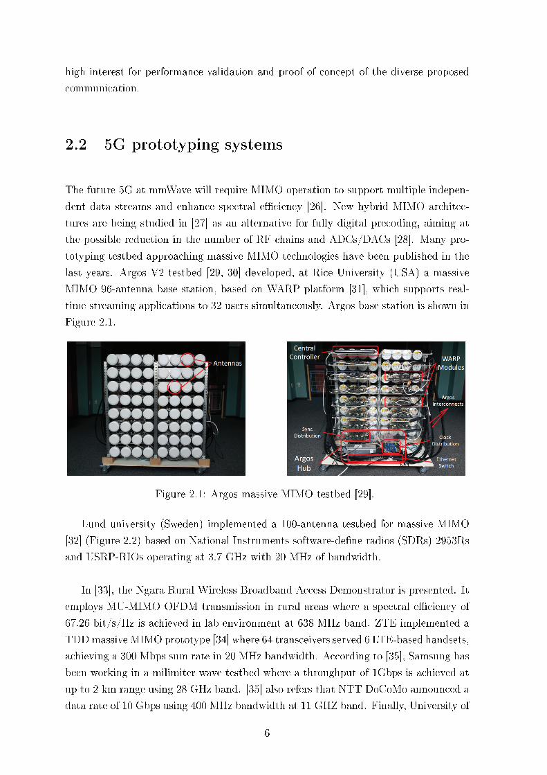
last years. Argos V2 testbed [29, 30] developed, at Rice University (USA) a massive
MIMO 96-antenna base station, based on WARP platform [31], which supports real-
time streaming applications to 32 users simultaneously. Argos base station is shown in
Figure 2.1.
Figure 2.1: Argos massive MIMO testbed [29].
Lund university (Sweden) implemented a 100-antenna testbed for massive MIMO
[32] (Figure 2.2) based on National Instruments software-dene radios (SDRs) 2953Rs
and USRP-RIOs operating at 3.7 GHz with 20 MHz of bandwidth.
In [33], the Ngara Rural Wireless Broadband Access Demonstrator is presented. It
employs MU-MIMO OFDM transmission in rural areas where a spectral eciency of
67.26 bit/s/Hz is achieved in lab environment at 638 MHz band. ZTE implemented a
TDDmassive MIMO prototype [34] where 64 transceivers served 6 LTE-based handsets,
achieving a 300 Mbps sum rate in 20 MHz bandwidth. According to [35], Samsung has
been working in a milimiter wave testbed where a throughput of 1Gbps is achieved at
up to 2 km range using 28 GHz band. [35] also refers that NTT DoCoMo announced a
data rate of 10 Gbps using 400 MHz bandwidth at 11 GHZ band. Finally, University of
6
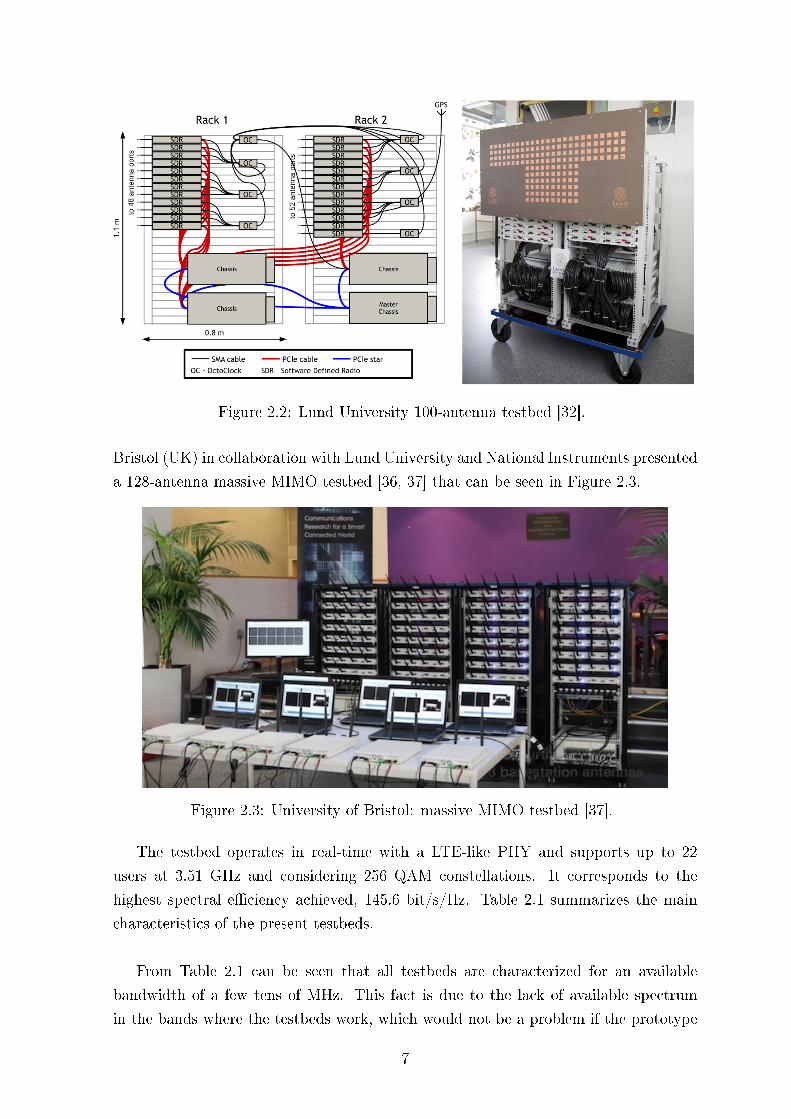
Figure 2.2: Lund University 100-antenna testbed [32].
Bristol (UK) in collaboration with Lund University and National Instruments presented
a 128-antenna massive MIMO testbed [36, 37] that can be seen in Figure 2.3.
Figure 2.3: University of Bristol: massive MIMO testbed [37].
The testbed operates in real-time with a LTE-like PHY and supports up to 22
users at 3.51 GHz and considering 256 QAM constellations. It corresponds to the
highest spectral eciency achieved, 145.6 bit/s/Hz. Table 2.1 summarizes the main
characteristics of the present testbeds.
From Table 2.1 can be seen that all testbeds are characterized for an available
bandwidth of a few tens of MHz. This fact is due to the lack of available spectrum
in the bands where the testbeds work, which would not be a problem if the prototype
7
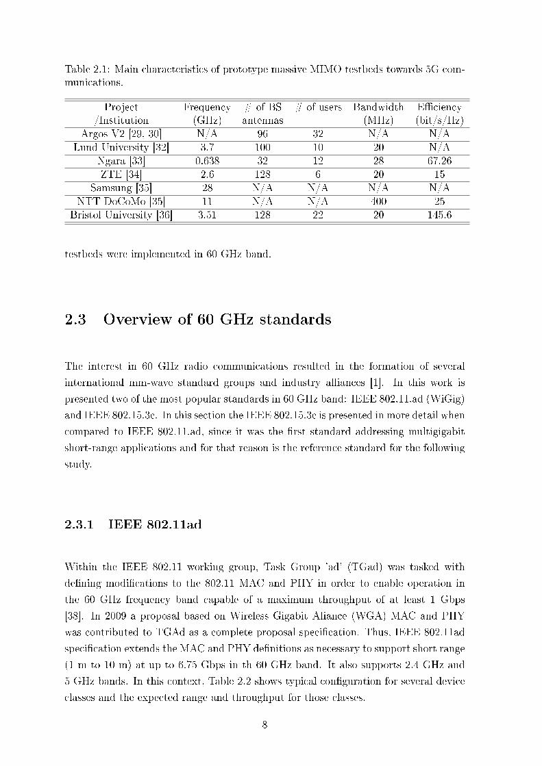
Table 2.1: Main characteristics of prototype massive MIMO testbeds towards 5G com-munications.
Project Frequency # of BS # of users Bandwidth Eciency/Institution (GHz) antennas (MHz) (bit/s/Hz)
Argos V2 [29, 30] N/A 96 32 N/A N/ALund University [32] 3.7 100 10 20 N/A
Ngara [33] 0.638 32 12 28 67.26ZTE [34] 2.6 128 6 20 15
Samsung [35] 28 N/A N/A N/A N/ANTT DoCoMo [35] 11 N/A N/A 400 25
Bristol University [36] 3.51 128 22 20 145.6
testbeds were implemented in 60 GHz band.
2.3 Overview of 60 GHz standards
The interest in 60 GHz radio communications resulted in the formation of several
international mm-wave standard groups and industry alliances [1]. In this work is
presented two of the most popular standards in 60 GHz band: IEEE 802.11.ad (WiGig)
and IEEE 802.15.3c. In this section the IEEE 802.15.3c is presented in more detail when
compared to IEEE 802.11.ad, since it was the rst standard addressing multigigabit
short-range applications and for that reason is the reference standard for the following
study.
2.3.1 IEEE 802.11ad
Within the IEEE 802.11 working group, Task Group 'ad' (TGad) was tasked with
dening modications to the 802.11 MAC and PHY in order to enable operation in
the 60 GHz frequency band capable of a maximum throughput of at least 1 Gbps
[38]. In 2009 a proposal based on Wireless Gigabit Aliance (WGA) MAC and PHY
was contributed to TGAd as a complete proposal specication. Thus, IEEE 802.11ad
specication extends the MAC and PHY denitions as necessary to support short range
(1 m to 10 m) at up to 6.75 Gbps in th 60 GHz band. It also supports 2.4 GHz and
5 GHz bands. In this context, Table 2.2 shows typical conguration for several device
classes and the expected range and throughput for those classes.
8
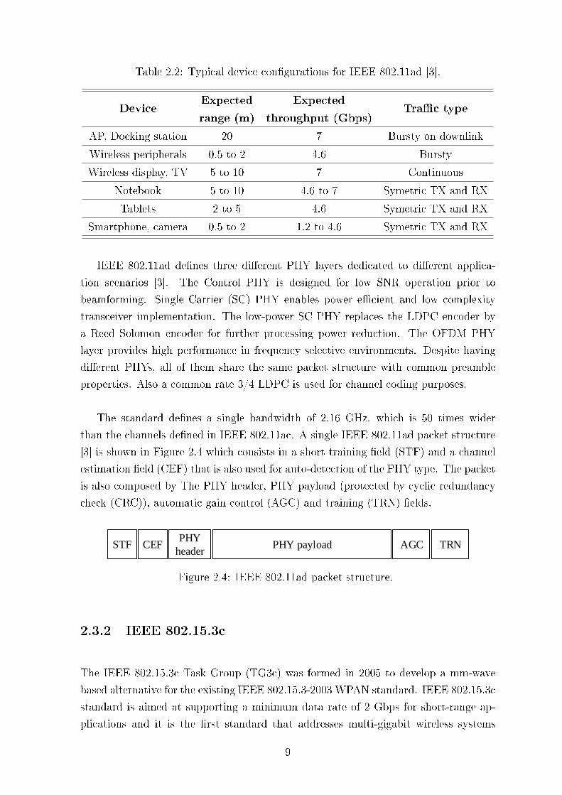
Table 2.2: Typical device congurations for IEEE 802.11ad [3].
DeviceExpected Expected
Trac typerange (m) throughput (Gbps)
AP, Docking station 20 7 Bursty on downlink
Wireless peripherals 0.5 to 2 4.6 Bursty
Wireless display, TV 5 to 10 7 Continuous
Notebook 5 to 10 4.6 to 7 Symetric TX and RX
Tablets 2 to 5 4.6 Symetric TX and RX
Smartphone, camera 0.5 to 2 1.2 to 4.6 Symetric TX and RX
IEEE 802.11ad denes three dierent PHY layers dedicated to dierent applica-
tion scenarios [3]. The Control PHY is designed for low SNR operation prior to
beamforming. Single Carrier (SC) PHY enables power ecient and low complexity
transceiver implementation. The low-power SC PHY replaces the LDPC encoder by
a Reed Solomon encoder for further processing power reduction. The OFDM PHY
layer provides high performance in frequency selective environments. Despite having
dierent PHYs, all of them share the same packet structure with common preamble
properties. Also a common rate 3/4 LDPC is used for channel coding purposes.
The standard denes a single bandwidth of 2.16 GHz, which is 50 times wider
than the channels dened in IEEE 802.11ac. A single IEEE 802.11ad packet structure
[3] is shown in Figure 2.4 which consists in a short training eld (STF) and a channel
estimation eld (CEF) that is also used for auto-detection of the PHY type. The packet
is also composed by The PHY header, PHY payload (protected by cyclic redundancy
check (CRC)), automatic gain control (AGC) and training (TRN) elds.
STF CEFPHY
headerPHY payload AGC TRN
Figure 2.4: IEEE 802.11ad packet structure.
2.3.2 IEEE 802.15.3c
The IEEE 802.15.3c Task Group (TG3c) was formed in 2005 to develop a mm-wave
based alternative for the existing IEEE 802.15.3-2003 WPAN standard. IEEE 802.15.3c
standard is aimed at supporting a minimum data rate of 2 Gbps for short-range ap-
plications and it is the rst standard that addresses multi-gigabit wireless systems
9
[1]. The 802.15.3c Task Group presents ve usage models (UMs) related to the possi-
ble consumer applications in the 60 GHz band [39]: UM 1) Uncompressed video
streaming: The bandwidth available in the 60 GHz band enables sending HDTV sig-
nals without the needing for video cables. It is expected a data rate over 3.5 Gbps in a
10 m range with a pixel error rate below 10−9. UM 2) Uncompressed multivideo
streaming: The 802.15.3c system should be able to provide video signals for at least
two 0.62 Gbps streams. UM 3) Oce desktop: This UM enables the communica-
tion between a personal computer and other external peripherals, including printers
and hard drives. UM 4) Conference and hadoc: This UM considers a scenario
where several computers are communicating between each other using one 802.15.3c
network. UM 5) kiosk le downloading: TG3c group assumed electronic kiosks
that enables, for example downloading video and music les at 1.5 Gbps at 1 m range.
The IEEE 802.15.3c channel modelling subcommittee has dened a new channel
model in regard of the Saleh-Valenzuela (S-V) model previously used in IEEE 802.11.
The new model combines a line-of-sight (LOS) component using a two-path model with
de NLOS reective clusters of the S-V model [40].
The target applications of the standard have dierent requirements and for that
reason 802.15.3c Task Group has developed three dierent PHY modes: Single Carrier
mode (SC PHY), High-Speed Interface mode (HSI PHY) and Audio-Visual mode (AV
PHY). The SC PHY is most suitable for oce desktop (UM3) and kiosk le down-
loading (UM5) usage models. The HSI PHY mode is designed for bidirectional, NLOS,
low-latency communication scenarios, which is the case of the conference and hadoc us-
age model (UM4). The AV PHY is designed to provide high throughput video streams
(usage models 1 and 2). A comparison of this three PHY modes is given in Table 2.3
[41].
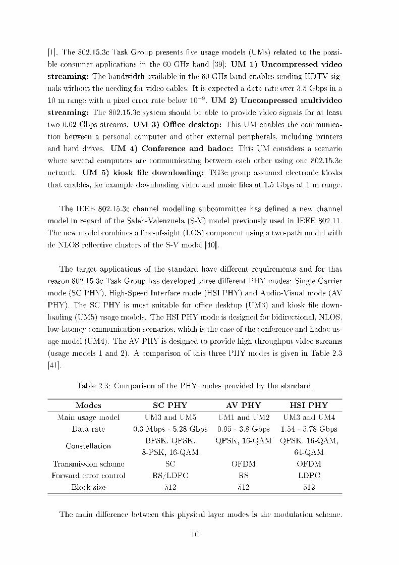
Table 2.3: Comparison of the PHY modes provided by the standard.
Modes SC PHY AV PHY HSI PHY
Main usage model UM3 and UM5 UM1 and UM2 UM3 and UM4
Data rate 0.3 Mbps - 5.28 Gbps 0.95 - 3.8 Gbps 1.54 - 5.78 Gbps
ConstellationBPSK, QPSK, QPSK, 16-QAM QPSK, 16-QAM,
8-PSK, 16-QAM 64-QAM
Transmission scheme SC OFDM OFDM
Forward error control RS/LDPC RS LDPC
Block size 512 512 512
The main dierence between this physical layer modes is the modulation scheme.
10
While SC PHY uses single carrier (SC) modulation, AV PHY and HSI PHY uses
OFDM. SC modulation allows lower complexity and low power operation, whereas
OFDM is more appropriated in high spectral eciency and NLOS channel conditions.
Further the three PHY layers are explained in detail according to [41] and [2].
2.3.2.1 Single Carrier PHY
SC PHY provides three classes of modulation and coding schemes (MCSs) focusing on
dierent wireless connectivity applications. Class 1 addresses kiosk le downloading
and low-power mobile market with data rates of up to 1.5 Gbps. Class 2 aims to
achieve data rates up to 3 Gbps and is dened for oce desktop. Class 3 is specied for
supporting high-performance applications with data rates exceeding 3 Gbps. The MCs
dependent parameters for SC PHY is shown in Appendix A. In SC PHY the support
of π/2-shifted binary phase shift keying (π/2 BPSK) is mandatory for all devices since
it improves the peak-to-average power ratio. Other supported modulation schemes are
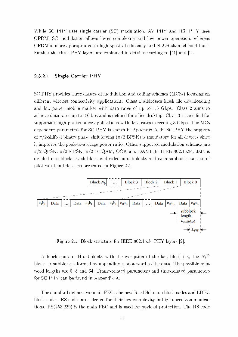
π/2 QPSK, π/2 8-PSK, π/2 16 QAM, OOK and DAMI. In IEEE 802.15.3c, data is
divided into blocks, each block is divided in subblocks and each subblock consists of
pilot word and data, as presented in Figure 2.5.
Figure 2.5: Block structure for IEEE 802.15.3c PHY layers [2].
A block contain 64 subblocks with the exception of the last block i.e., the Nbth
block. A subblock is formed by appending a pilot word to the data. The possible pilot
word lengths are 0, 8 and 64. Frame-related parameters and time-related parameters
for SC PHY can be found in Appendix A.
The standard denes two main FEC schemes: Reed Solomon block codes and LDPC
block codes. RS codes are selected for their low complexity in high-speed communica-
tions. RS(255,239) is the main FEC and is used for payload protection. The RS code
11
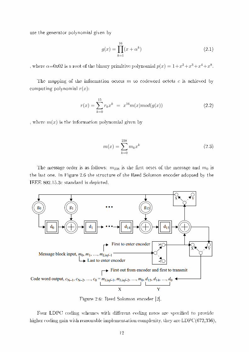
use the generator polynomial given by
g(x) =16∏k=1
(x+ αk) (2.1)
, where α=0x02 is a root of the binary primitive polynomial p(x) = 1+x2 +x3 +x4 +x8.
The mapping of the information octets m to codeword octets c is achieved by
computing polynomial r(x):
r(x) =15∑k=0
rkxk = x16m(x)mod(g(x)) (2.2)
, where m(x) is the information polynomial given by
m(x) =238∑k=0
mkxk (2.3)
The message order is as follows: m238 is the rst octet of the message and m0 is
the last one. In Figure 2.6 the structure of the Reed Solomon encoder adopted by the
IEEE 802.15.3c standard is depicted.
Figure 2.6: Reed Solomon encoder [2].
Four LDPC coding schemes with dierent coding rates are specied to provide
higher coding gain with reasonable implementation complexity, they are LDPC(672,336),
12
LDPC(672,504), LDPC(672,588) and LDPC (1440,1344). The LDPC encoder is sys-
tematic, i.e., it encodes an information block of size k, i = (i0, i1, ..., ik−1) into a code-
word c of size n, where c = (i0, i1, ..., ik−1, p0, p1, ..., pk−1), by adding n − k parity bits
obtained so that HcT = 0, where H is an (n− k)× n parity check matrix.
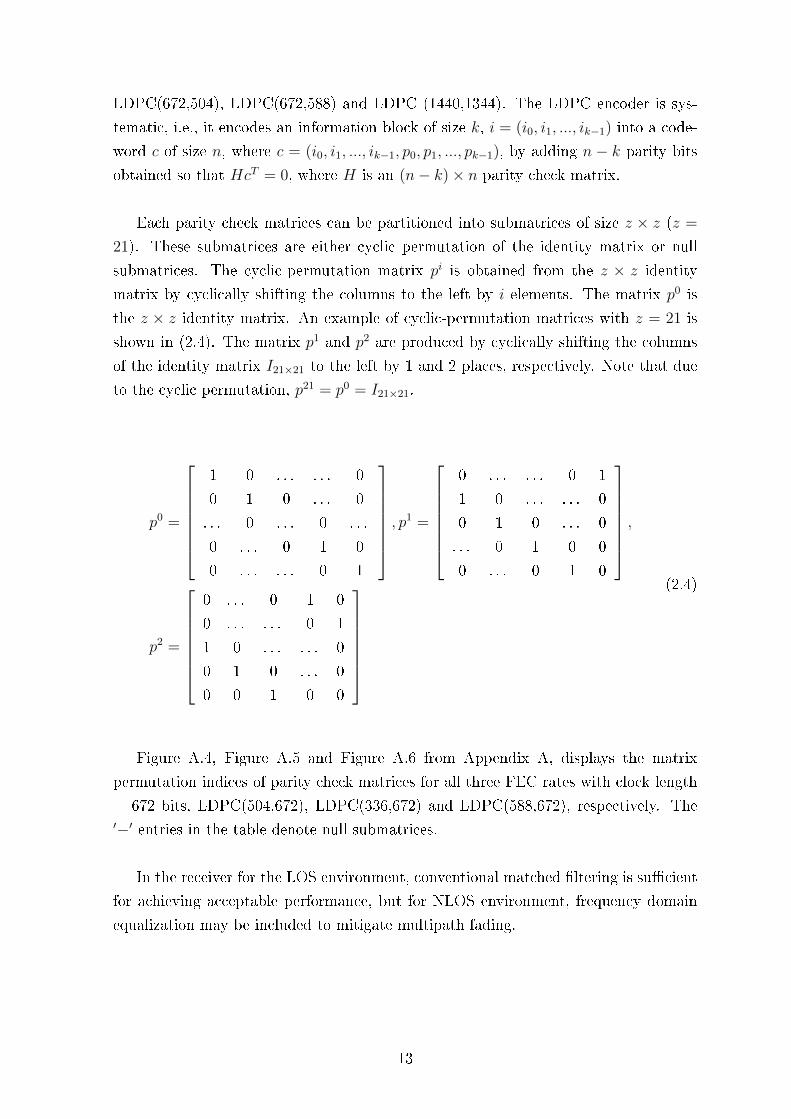
Each parity check matrices can be partitioned into submatrices of size z × z (z =
21). These submatrices are either cyclic permutation of the identity matrix or null
submatrices. The cyclic-permutation matrix pi is obtained from the z × z identity
matrix by cyclically shifting the columns to the left by i elements. The matrix p0 is
the z × z identity matrix. An example of cyclic-permutation matrices with z = 21 is
shown in (2.4). The matrix p1 and p2 are produced by cyclically shifting the columns
of the identity matrix I21×21 to the left by 1 and 2 places, respectively. Note that due
to the cyclic permutation, p21 = p0 = I21×21.
p0 =
1 0 . . . . . . 0
0 1 0 . . . 0
. . . 0 . . . 0 . . .
0 . . . 0 1 0
0 . . . . . . 0 1
, p1 =
0 . . . . . . 0 1
1 0 . . . . . . 0
0 1 0 . . . 0
. . . 0 1 0 0
0 . . . 0 1 0
,
p2 =
0 . . . 0 1 0
0 . . . . . . 0 1
1 0 . . . . . . 0
0 1 0 . . . 0
0 0 1 0 0
(2.4)
Figure A.4, Figure A.5 and Figure A.6 from Appendix A, displays the matrix
permutation indices of parity check matrices for all three FEC rates with clock length
= 672 bits, LDPC(504,672), LDPC(336,672) and LDPC(588,672), respectively. The′−′ entries in the table denote null submatrices.
In the receiver for the LOS environment, conventional matched ltering is sucient
for achieving acceptable performance, but for NLOS environment, frequency domain
equalization may be included to mitigate multipath fading.
13
2.3.2.2 Audio/Visual PHY
Within AV PHY two dierent sub-PHY modes are considered: high-rate PHY (HRP)
for video transmission and low-rate PHY (LRP) for the control signal. Both sub-
PHY use OFDM. The HRP mode has an FFT length of 512 and uses all the channel
bandwidth available, delivering data rates of 0.952, 1.904 and 3.807 Gbps as can be seen
in Appendix B.1. On the other hand, the LRP mode occupies only 98 MHz bandwidth
and three LRPs are arranged per HRP channel. This allocation aims to accommodate
three dierent networks in one channel.
The AV PHY uses RS codes as the outer code and convolutional coding as the inner
code in HRP mode. Only convolutional coding is used in LRP mode. The convolutional
encoder considered in this PHY layer use length K = 7, delay memory 6, generator
polyonmial g0 = 133o, g1 = 171o, g2 = 165o and code rate 1/3.
Modulation schemes used are limited to QPSK and 16 QAM and the corresponding
modulation parameter are presented in Appendix B.2.
2.3.2.3 High-Speed Interface PHY
As stated before, the HSI PHY is designed mainly for computer peripherals that require
low-latency bidirectional data, focusing on the conference hadoc UM, and uses OFDM,
where the FFT size is 512.
As OFDM modulation has an inherent complexity due to the IFFT and FFT op-
erations, only the LDPC coding scheme is used in the HSI PHY. Four FEC rates are
obtained using LDPC(336,672), LDPC(504,672), LDPC(588,672) and LDPC(420,672)
codes which allows code rates of 1/2, 5/8, 7/8 and 3/4, receptively. The LDPC en-
coding process for HSI PHY is the same as explained in Section 2.3.2.1 where the rst
three matrix permutation of the block codes for HSI were introduced. The matrix per-
mutation indices of the parity check matrix for LDPC(420,672) is depicted in Appendix
C.4.
In terms of modulation, three modulation schemes are selected: QPSK, 16 QAM
and 64 QAM, which allow data rates up to 5.775 Gbps, as can be seen in detail in
Appendix C.1. The standard suggests that the conversion from binary data to complex
symbols shall be performed according to Gray-coded constellation mapping as shown
14
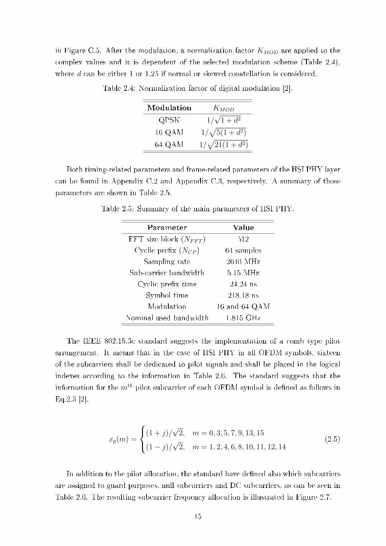
in Figure C.5. After the modulation, a normalization factor KMOD are applied to the
complex values and it is dependent of the selected modulation scheme (Table 2.4),
where d can be either 1 or 1.25 if normal or skewed constellation is considered.
Table 2.4: Normalization factor of digital modulation [2].
Modulation KMOD
QPSK 1/√
1 + d2
16 QAM 1/√
5(1 + d2)
64 QAM 1/√
21(1 + d2)
Both timing-related parameters and frame-related parameters of the HSI PHY layer
can be found in Appendix C.2 and Appendix C.3, respectively. A summary of those
parameters are shown in Table 2.5.
Table 2.5: Summary of the main parameters of HSI PHY.
Parameter Value
FFT size block (NFFT ) 512
Cyclic prex (NCP ) 64 samples
Sampling rate 2640 MHz
Sub-carrier bandwidth 5.15 MHz
Cyclic prex time 24.24 ns
Symbol time 218.18 ns
Modulation 16 and 64 QAM
Nominal used bandwidth 1.815 GHz
The IEEE 802.15.3c standard suggests the implementation of a comb type pilot
arrangement. It means that in the case of HSI PHY in all OFDM symbols, sixteen
of the subcarriers shall be dedicated to pilot signals and shall be placed in the logical
indexes according to the information in Table 2.6. The standard suggests that the
information for the mth pilot subcarrier of each OFDM symbol is dened as follows in
Eq.2.5 [2].
xp(m) =
(1 + j)/√
2, m = 0, 3, 5, 7, 9, 13, 15
(1− j)/√
2, m = 1, 2, 4, 6, 8, 10, 11, 12, 14(2.5)
In addition to the pilot allocation, the standard have dened also which subcarriers
are assigned to guard purposes, null subcarriers and DC subcarriers, as can be seen in
Table 2.6. The resulting subcarrier frequency allocation is illustrated in Figure 2.7.
15
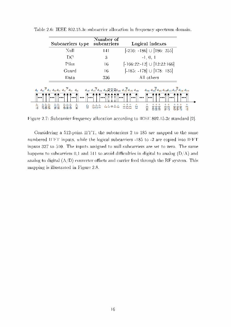
Table 2.6: IEEE 802.15.3c subcarrier allocation in frequency spectrum domain.
Subcarriers typeNumber ofsubcarriers Logical indexes
Null 141 [-256: -186] ∪ [186: 255]
DC 3 -1, 0, 1
Pilot 16 [-166:22:-12] ∪ [12:22:166]
Guard 16 [-185: -178] ∪ [178: 185]
Data 336 All others
Figure 2.7: Subcarrier frequency allocation according to IEEE 802.15.3c standard [2].
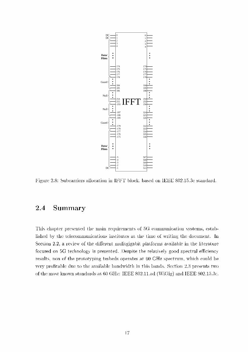
Considering a 512-point IFFT, the subcarriers 2 to 185 are mapped to the same
numbered IFFT inputs, while the logical subcarriers -185 to -2 are copied into IFFT
inputs 327 to 510. The inputs assigned to null subcarriers are set to zero. The same
happens to subcarriers 0,1 and 511 to avoid diculties in digital to analog (D/A) and
analog to digital (A/D) converter osets and carrier feed through the RF system. This
mapping is illustrated in Figure 2.8.
16
IFFT
DCDC
Data/
Pilots
Guard
Null
Null
Guard
Data/
Pilots
DC
0
1
2
3
4
177
178
185
186
255
254
184
176
175
174
-255
-187
-186
-185
-178
-179
-1
-2
-3
-4
-5
-177
-176
-175
0
1
2
3
4
324
325
326
333
332
511
510
509
508
507
334
335
336
177
178
185
186
255
254
184
176
175
174
256
Figure 2.8: Subcarriers allocation in IFFT block, based on IEEE 802.15.3c standard.
2.4 Summary
This chapter presented the main requirements of 5G communication systems, estab-
lished by the telecommunications institutes at the time of writing the document. In
Section 2.2, a review of the dierent mulitgigabit platforms available in the literature
focused on 5G technology is presented. Despite the relatively good spectral eciency
results, non of the prototyping tesbeds operates at 60 GHz spectrum, which could be
very protable due to the available bandwidth in this bands. Section 2.3 presents two
of the most known standards at 60 GHz: IEEE 802.11.ad (WiGig) and IEEE 802.15.3c.
17

18

Chapter 3
Theoretical Fundamentals
3.1 Introduction to OFDM
Orthogonal Frequency Division Multiplexing (OFDM) is a modulation scheme that is
widely used for high data rate transmission in delay dispersive environments, since it
split a frequency-selective channel bandwidth into several at sub-bands [42]. High
data rate transmission schemes usually employs single-carrier or multicarrier systems.
Since in this work, a multicarrier approach is explored (OFDM), a comparison between
those approaches is described next.
3.1.1 Single-carrier vs. multicarrier systems
In a single-carrier system, the transmitted symbol an are pulse-shaped by a transmit
lter gT (t) in the transmitter. The period of each symbol is T seconds, which is
translated in a data rate of R = 1/T . Consider a band-limited channel h(t) with
an available bandwidth W . After receiving the symbols through the channel they
are processed in the received lter, as shown in Figure 3.1. Let gT (t), gR(t), and
h−1(t) denote the impulse response of the transmit lter, receive lter and equalizer,
respectively.
Figure 3.1: Single-carrier baseband communication system [43].
19
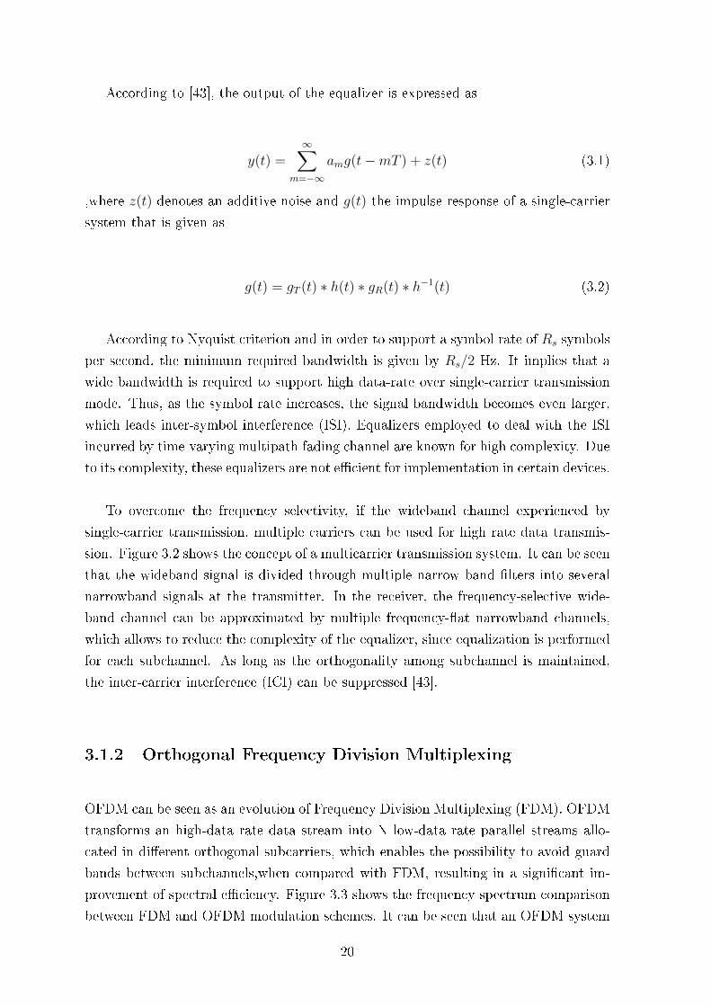
According to [43], the output of the equalizer is expressed as
y(t) =∞∑
m=−∞
amg(t−mT ) + z(t) (3.1)
,where z(t) denotes an additive noise and g(t) the impulse response of a single-carrier
system that is given as
g(t) = gT (t) ∗ h(t) ∗ gR(t) ∗ h−1(t) (3.2)
According to Nyquist criterion and in order to support a symbol rate of Rs symbols
per second, the minimum required bandwidth is given by Rs/2 Hz. It implies that a
wide bandwidth is required to support high data-rate over single-carrier transmission
mode. Thus, as the symbol rate increases, the signal bandwidth becomes even larger,
which leads inter-symbol interference (ISI). Equalizers employed to deal with the ISI
incurred by time-varying multipath fading channel are known for high complexity. Due
to its complexity, these equalizers are not ecient for implementation in certain devices.
To overcome the frequency selectivity, if the wideband channel experienced by
single-carrier transmission, multiple carriers can be used for high rate data transmis-
sion. Figure 3.2 shows the concept of a multicarrier transmission system. It can be seen
that the wideband signal is divided through multiple narrow band lters into several
narrowband signals at the transmitter. In the receiver, the frequency-selective wide-
band channel can be approximated by multiple frequency-at narrowband channels,
which allows to reduce the complexity of the equalizer, since equalization is performed
for each subchannel. As long as the orthogonality among subchannel is maintained,
the inter-carrier interference (ICI) can be suppressed [43].
3.1.2 Orthogonal Frequency Division Multiplexing
OFDM can be seen as an evolution of Frequency Division Multiplexing (FDM). OFDM
transforms an high-data rate data stream into N low-data rate parallel streams allo-
cated in dierent orthogonal subcarriers, which enables the possibility to avoid guard
bands between subchannels,when compared with FDM, resulting in a signicant im-
provement of spectral eciency. Figure 3.3 shows the frequency spectrum comparison
between FDM and OFDM modulation schemes. It can be seen that an OFDM system
20
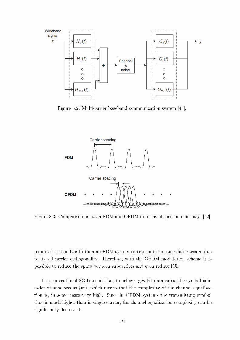
Figure 3.2: Multicarrier baseband communication system [43].
Figure 3.3: Comparison between FDM and OFDM in terms of spectral eciency. [42]
requires less bandwidth than an FDM system to transmit the same data stream, due
to its subcarrier orthogonality. Therefore, with the OFDM modulation scheme it is
possible to reduce the space between subcarriers and even reduce ICI.
In a conventional SC transmission, to achieve gigabit data rates, the symbol is in
order of nano-secons (ns), which means that the complexity of the channel equaliza-
tion is, in some cases very high. Since in OFDM systems the transmitting symbol
time is much higher than in single carrier, the channel equalization complexity can be
signicantly decreased.
21
3.1.2.1 M-ary Digital Modulation
Digital modulation is the mapping of data bits into signal waveforms that can be
transmitted over a channel [42]. At the transmitter (TX) the digital modulator has to
convert the digital source data into analog waveforms, while at the receiver (RX), the
demodulator recovers the bits from the received waveform.
An analog waveform can represent either one bit or a group of bits, depending of
the modulation typology. Generally, a group of K bits can be encoded in to a symbol,
which is mapped into one out of a set of M = 2K waveforms. Typically, the waveform
corresponding to one symbol is time limited to a time TS. Therefore, the bit rate is K
times the transmission symbol rate.
A typical example of two digital modulation methods are QPSK and QAM. QPSK
is a characterized for four (M = 4) dierent waveforms, which result in two (K = 2)
bits per symbol. Thus the modulated signal is function of the carrier phase and is
given by Eq.3.3.
si(t) =
√2EsTs
cos(2πfc + (2n− 1)π
4), n = 1, 2, 3, 4 (3.3)
,where√Es is the energy per symbol and fc is the carrier frequency.
This yield the four phases π4, 3π
4, 5π
4and 7π
4and can be represented in a two-
dimensional signal space as in Eq.3.4 and Eq.3.5.
φ1(t) =
√2
Tscos(2πfct) (3.4)
φ1(t) =
√2
Tssin(2πfct) (3.5)
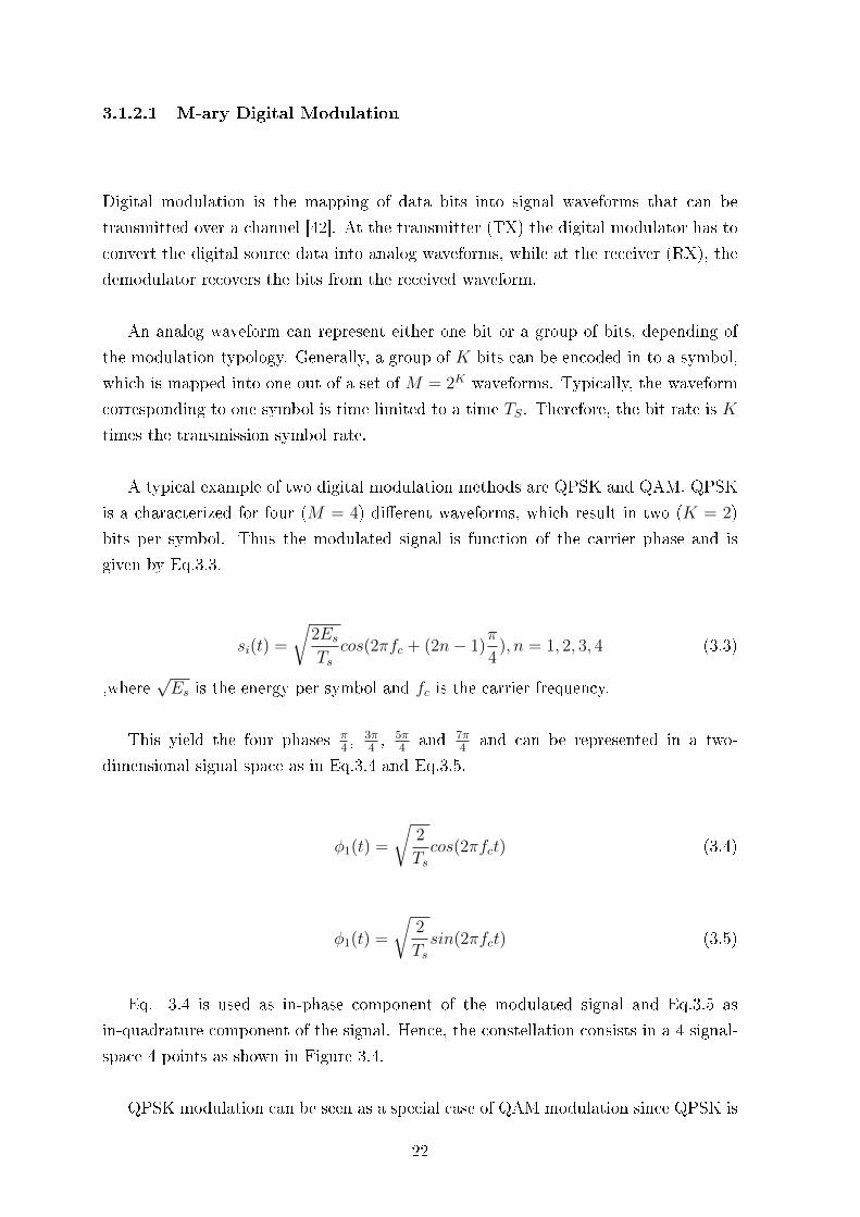
Eq. 3.4 is used as in-phase component of the modulated signal and Eq.3.5 as
in-quadrature component of the signal. Hence, the constellation consists in a 4 signal-
space 4 points as shown in Figure 3.4.
QPSK modulation can be seen as a special case of QAM modulation since QPSK is
22
I
Q
1101
00 10
Figure 3.4: QPSK constellation.
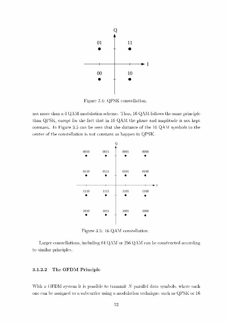
not more than a 4 QAM modulation scheme. Thus, 16 QAM follows the same principle
than QPSK, except for the fact that in 16 QAM the phase and amplitude is not kept
constant. In Figure 3.5 can be seen that the distance of the 16 QAM symbols to the
center of the constellation is not constant as happen in QPSK.
I
Q
0010
0110
0011 0001 0000
010001010111
1110 1111 1101 1100
1010 1011 1001 1000
Figure 3.5: 16 QAM constellation.
Larger constellations, including 64 QAM or 256 QAM can be constructed according
to similar principles.
3.1.2.2 The OFDM Principle
With a OFDM system it is possible to transmit N parallel data symbols, where each
one can be assigned to a subcarrier using a modulation technique, such as QPSK or 16
23
QAM. The data rate per subcarrier is as slower as the number of subcarriers available in
the system, increasing the transmission symbol time in each subcarrier. This fact leads
to a lower complexity in the receiver since the consequences of a frequency selective
channel are mitigated.
Let Xn, n = 0, 1, ..., N − 1, be the N data symbols to be transmitted over N
subcarriers, where Xn is represented as a complex point in a QAM modulation, for
example and fn be the frequency for the nth subcarrier. The transmitted waveform in
time-domain can be written as [1]
x(t) =N−1∑n=0
Xnej2πfnt (3.6)
and the corresponding digitally sampled version is given by
x(mTs) =N−1∑n=0
Xnej2πfnmTs (3.7)
, where t = mTs represents the sampling points and Ts the sampling period. Consid-
ering that the N subcarriers are equally spaced in frequency domain that fn = nfo ,
Eq. 3.8 becomes
x(mTs) =N−1∑n=0
Xnej2πnfomTs (3.8)
, where fo = 1/NTs is the minimum frequency separation to ensure subcarrier orthog-
onality. Thus, the time-domain samples can be written as
x(mTs) =N−1∑n=0
Xnej2πmn/N (3.9)
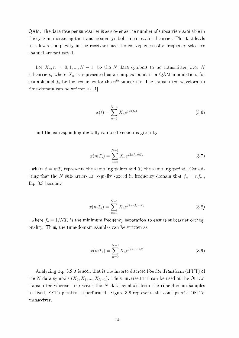
Analyzing Eq. 3.9 it is seen that is the Inverse discrete Fourier Transform (IFFT) of
the N data symbols (X0, X1, ..., XN−1). Thus, inverse FFT can be used at the OFDM
transmitter whereas to recover the N data symbols from the time-domain samples
received, FFT operation is performed. Figure 3.6 represents the concept of a OFDM
transceiver.
24
Data
source
Serial to
ParallelIFFT
Parallel
to SerialH
Serial to
ParallelFFT
Parallel
to SerialData sink
Transmitter ReceiverChannel
0
1
2
N-2
N-1
0
1
2
N-2
N-1
Figure 3.6: Transceiver structure of an OFDM system
CPOFDM symbol OFDM symbolCP CP
TCP TS TCP TS
TOFDM TOFDM
Figure 3.7: Principle of the cyclic prex.
3.1.2.3 Cyclic Prex
As already discussed, an OFDM system aims to reduce the negative eects of an high
data rate transmission over frequency selective channels, by increasing the symbol time
in each subcarrier. However, the eect of delayed OFDM symbols can lead to the loss of
orthogonality among subcarriers, increasing ISI and consequently increasing Bit Error
Rate (BER).
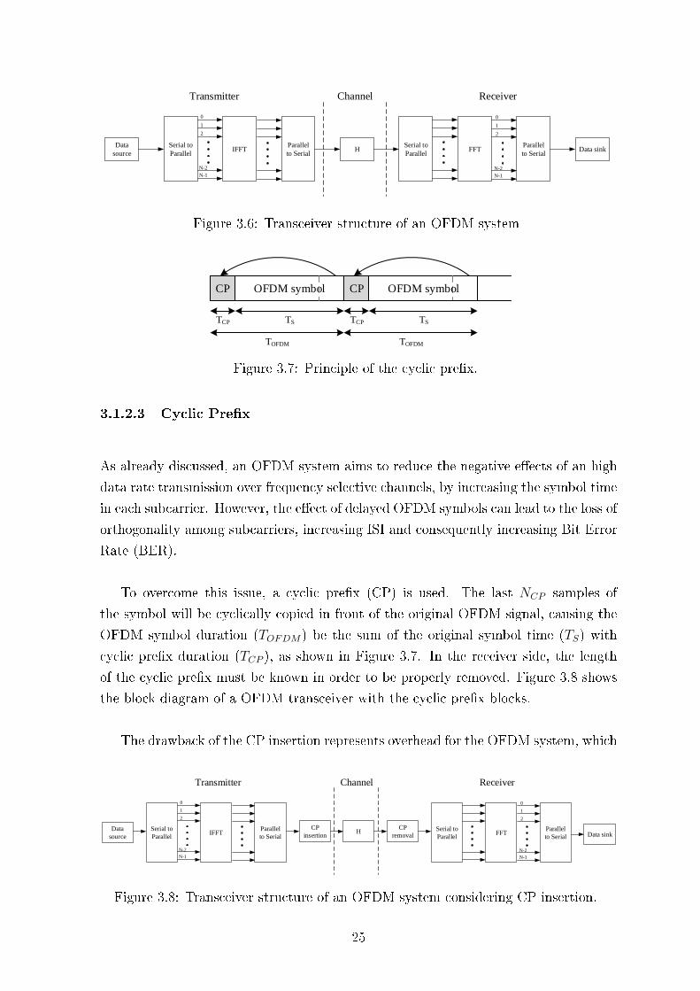
To overcome this issue, a cyclic prex (CP) is used. The last NCP samples of
the symbol will be cyclically copied in front of the original OFDM signal, causing the
OFDM symbol duration (TOFDM) be the sum of the original symbol time (TS) with
cyclic prex duration (TCP ), as shown in Figure 3.7. In the receiver side, the length
of the cyclic prex must be known in order to be properly removed. Figure 3.8 shows
the block diagram of a OFDM transceiver with the cyclic prex blocks.
The drawback of the CP insertion represents overhead for the OFDM system, which
Data
source
Serial to
ParallelIFFT
Parallel
to SerialH Serial to
ParallelFFT
Parallel
to Serial Data sink
Transmitter ReceiverChannel
0
1
2
N-2
N-1
0
1
2
N-2
N-1
CP
removal
CP
insertion
Figure 3.8: Transceiver structure of an OFDM system considering CP insertion.
25
results in loss of energy (Eq. 3.10) eciency and system throughput that must be
considered [44]. This loss of energy ecient is due to fact that redundant information
is being transmitted, increasing the overhead of the system.
LCP = 10log10(TOFDMTS
) [dB] (3.10)
3.2 Mobile wireless multipath fading channels
The performance of mobile wireless communication systems is strongly dependent by
the wireless channel environment. As opposed to the typically static and predictable
characteristics of a wired channel, the wireless channel is dynamic and unpredictable,
which makes an exact analysis of the wireless system often dicult [43].
In wireless communications, radio waves are mainly aected by three dierent
modes of physical phenomena: reection, diraction and scattering [45], [46]. Re-
ection occurs when propagating wave impinges upon an object with large dimensions
compared to the wavelength, for example, surface of earth or a building. Diraction
occurs when the radio path between transmitter and the receiver is obstructed by a
surface with sharp irregularities or small openings. Scattering is the phenomena that
forces the radiation of an electromagnetic wave to deviate from a straight path by one
or more obstacles, with small dimensions compared to the wavelength. Those obstacles
such as street signs or lamp posts are referred to as the scatters.
One of the main source of signal degradation in a wireless channel is a phenomenon
called fading, the variation of the signal amplitude over time and frequency domains.
Fading may either due to multipath propagation, or to shadowing from obstacles that
aect the propagation of a radio wave. the fading phenomenon can be classied into
two dierent types: large-scale fading and small-scale fading. Large-scale fading occurs
as the mobile moves through a large distance. It is caused by path loss of signal as a
function of distance and shadowing by large objects. Small-scale fading refers to rapid
variation of signal levels due to the interference of multiple signal paths (multi-paths)
when the mobile station moves short distances.
The frequency selectivity of a channel is characterized (e.g., by frequency-selective
or frequency at) for small-scale fading. Meanwhile, depending on the time variation
in a channel due to mobile speed (characterized by Doppler spread) short-term fading
26
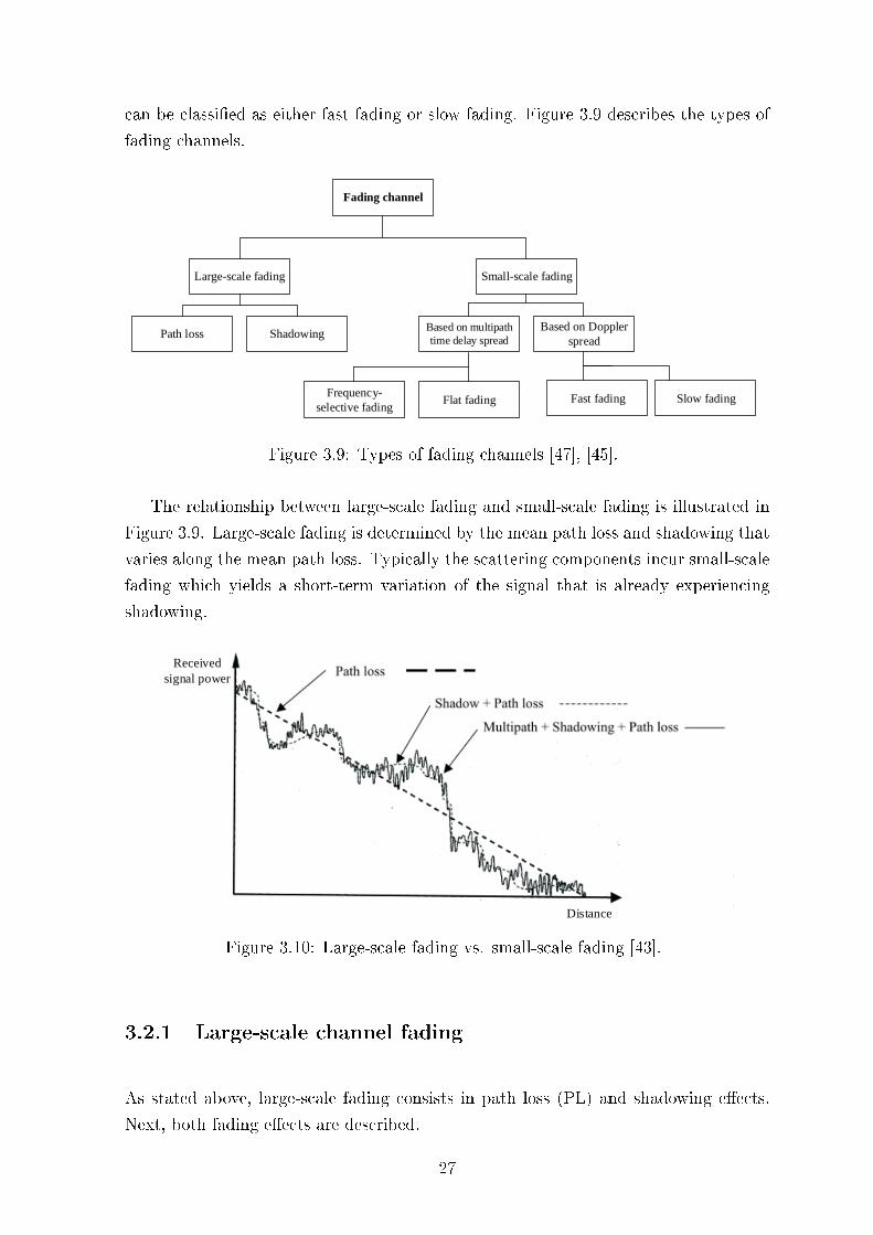
can be classied as either fast fading or slow fading. Figure 3.9 describes the types of
fading channels.
Fading channel
Large-scale fading Small-scale fading
Path loss ShadowingBased on multipath
time delay spread
Based on Doppler
spread
Frequency-
selective fadingFlat fading Fast fading Slow fading
Figure 3.9: Types of fading channels [47], [45].
The relationship between large-scale fading and small-scale fading is illustrated in
Figure 3.9. Large-scale fading is determined by the mean path loss and shadowing that
varies along the mean path loss. Typically the scattering components incur small-scale
fading which yields a short-term variation of the signal that is already experiencing
shadowing.
Distance
Received
signal power
Figure 3.10: Large-scale fading vs. small-scale fading [43].
3.2.1 Large-scale channel fading
As stated above, large-scale fading consists in path loss (PL) and shadowing eects.
Next, both fading eects are described.
27
3.2.1.1 Path loss
The path loss is dened as the ratio of the received signal power to the transmit signal
power, which describes the attenuation of the mean power as function of distance
between transmitter and receiver. In particular, at mmWave frequencies, the PL is
much more severe than at lower frequencies since the free space, for example at 60
GHz, PL increases approximately 22 dB compared to 5 GHz band [1]. Additionally,
the path loss at 60 GHz is subjected to additional losses due to oxygen absorption and
rain attenuation. This conditions makes 60 GHz bandwidth a promising candidate for
multi-gigabit wireless transmission for indoor rather than outdoor applications.
According to [1] and ignoring the PL frequency dependency, the PL as function of
distance, d can be given by
PL(d) = PL(d) +Xσ [dB], (3.11)
, where PL(d) denotes the average PL and Xσ represents the shadowing fading. In
general, PL(d) is expressed as
PL(d) = PL(d0) + 10nlog10(d
d0
) +
Q∑q=1
Xq [dB], for d ≥ d0, (3.12)
, where d0 and n denote the reference distance and PL exponent, respectively. Typically,
d0 = 1 m is used as the reference. The term Xq account for the additional attenuation
due to specic obstruction by objects.
3.2.1.2 Shadowing
Shadowing eect describes the average signal power receiver over a large area (a few
tens of wavelengths) due to the dynamic evolution of propagation paths, whereby new
paths arise and old paths disappear [1]. Due to the variation in the environment, the
received signal power will be dierent from the mean value for a given distance, which
causes the PL variation about the mean of PL value, as shown in 3.12.
Several measurements have shown that the shadowing fading is log-normally dis-
tributed, thus Xq denotes a zero-mean Gaussian random variable with standard devi-
28
ation σS [48]. The value of σS is always referred to a specic environment.
3.2.2 Small-scale channel fading and multipath
Small-scale fading is caused by the multipath signals that arrive at the receiver with
random phases that add constructively or destructively. It causes rapid changes in
signal strength over a small travel distance or time interval, it causes random frequency
modulation due to the varying Doppler shifts on dierent multipath signals, and nally
it can cause time dispersion (echoes) caused by multipath propagation delays.
There are many physical factors in radio propagation channels that inuence small-
scale fading of which stands out the multipath propagation, speed of the mobile and
the surrounding objects and the transmission bandwidth of the signal [45].
Next, several parameters that helps to characterize a small-scale channel fading and
the multipath phenomenon are described.
3.2.2.1 Doppler shift
Due to the relative motion between a mobile and a base station, each multipath wave
experiences a shift in frequency. This shift in received signal frequency is called Doppler
shift and it is directly proportional to the velocity and direction of motion of the mobile
relatively to the direction of arrival of the received multipath wave.
Considering a mobile moving at a constant velocity v and angle between the direc-
tion of the mobile's motion and the direction of arrival of the wave θ (Figure 3.11), the
Doppler shift fd is given by (3.13)
fd =v
λcos(θ) (3.13)
,where λ denotes the wavelength which is
λ =c
fc(3.14)
,where c is the velocity of the light and fc represents the transmitter operating frequency
29
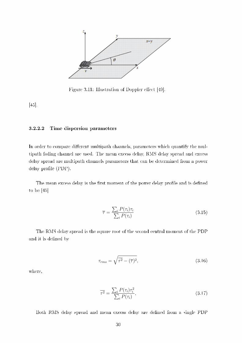
Figure 3.11: Illustration of Doppler eect [49].
[45].
3.2.2.2 Time dispersion parameters
In order to compare dierent multipath channels, parameters which quantify the mul-
tipath fading channel are used. The mean excess delay, RMS delay spread and excess
delay spread are multipath channels parameters that can be determined from a power
delay prole (PDP).
The mean excess delay is the rst moment of the power delay prole and is dened
to be [45]
τ =
∑i P (τi)τi∑i P (τi)
(3.15)
The RMS delay spread is the square root of the second central moment of the PDP
and it is dened by
τrms =
√τ 2 − (τ)2, (3.16)
where,
τ 2 =
∑i P (τi)τ
2i∑
i P (τi), (3.17)
Both RMS delay spread and mean excess delay are dened from a single PDP
30
which is the temporal or spatial average of consecutive impulse response measurements
collected and averaged over a local area.
The maximum excess delay (τmax) of the PDP is dened to be the time delay during
which multipath energy is x dB below the strongest arriving multipath signal.
3.2.2.3 Coherence bandwidth
The Bc is a key metric involved in expressing the performance of any digital wireless
system over a fading channel, since if the system requires a bandwidth larger than Bc
of the channel, amplitude and phase distortion of the signal will occur. In this case, the
fading channel is considered as a frequency-selective fading, making the digitally mod-
ulated data experience ISI. Coherence bandwidth is normally dened as the maximum
frequency dierence at which two signals are highly correlated and a correlation of 0.9
(Bc0.9) is most commonly used. It can be calculated by (3.18), which is the Frequency
Correlation Function (FCF).
ρ(n) =N−h−1∑n=0
H(n)H∗(n+ h) (3.18)
where, H(n) is the complex transfer function of the channel, h represents the fre-
quency shift, ∗ denotes the complex conjugate and N is the number of channel realiza-
tions.
According to [45], the coherence bandwidth can also be related with the RMS delay
spread as
Bc0.9 =1
50τrms(3.19)
3.2.2.4 Doppler spread and coherence time
Doppler spread and coherence time are parameters used to describe the time varying
nature of the channel in a small-scale region. Doppler spread BD is dened as a range
of frequencies over which the received Doppler spectrum is non-zero. If the baseband
31
signal bandwidth is much greater than BD the eects of Doppler spread are negligible
at the receiver, which means a slow fading channel. Coherence time is the time domain
dual of Doppler spread and is used to characterize the time varying nature of the
frequency dispersiveness of the channel in time domain. In other words, coherence
time measures the time duration over which the channel impulse response is considered
invariant. According to [45] and [50] the coherence time (Tcoh) can be approximated to
Tcoh ≈1
2fd(3.20)
, where fd denotes the Doppler shift.
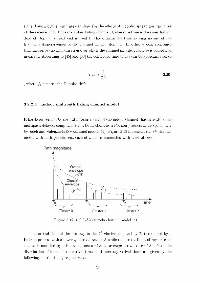
3.2.2.5 Indoor multipath fading channel model
It has been veried by several measurements of the indoor channel that arrivals of the
multipath-delayed components can be modeled as a Poisson process, more specically
by Saleh and Valenzuela (SV)channel model [51]. Figure 3.12 illustrates the SV channel
model with multiple clusters, each of which is associated with a set of rays.
Figure 3.12: Saleh-Valenzuela channel model [51].
The arrival time of the rst ray in the lth cluster, denoted by Tl is modeled by a
Poisson process with an average arrival rate of Λ while the arrival times of rays in each
cluster is modeled by a Poisson process with an average arrival rate of λ. Thus, the
distribution of inter-cluster arrival times and inter-ray arrival times are given by the
following distributions, respectively:
32
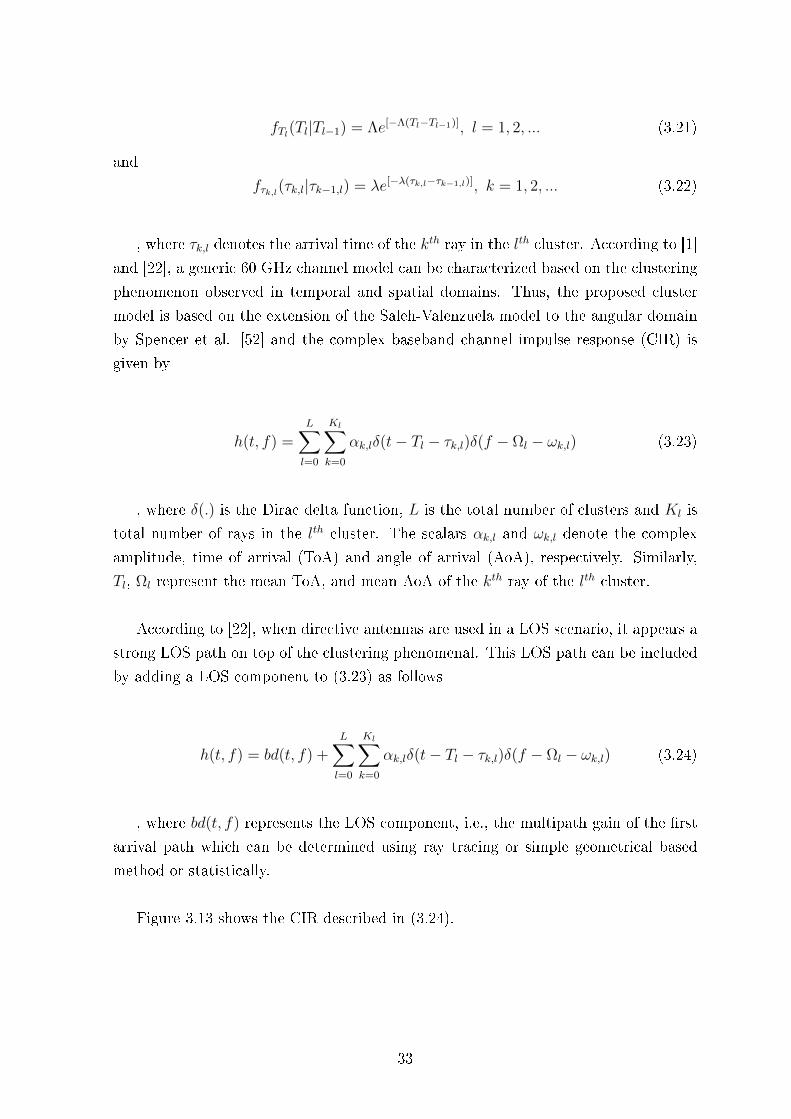
fTl(Tl|Tl−1) = Λe[−Λ(Tl−Tl−1)], l = 1, 2, ... (3.21)
and
fτk,l(τk,l|τk−1,l) = λe[−λ(τk,l−τk−1,l)], k = 1, 2, ... (3.22)
, where τk,l denotes the arrival time of the kth ray in the lth cluster. According to [1]
and [22], a generic 60 GHz channel model can be characterized based on the clustering
phenomenon observed in temporal and spatial domains. Thus, the proposed cluster
model is based on the extension of the Saleh-Valenzuela model to the angular domain
by Spencer et al. [52] and the complex baseband channel impulse response (CIR) is
given by
h(t, f) =L∑l=0
Kl∑k=0
αk,lδ(t− Tl − τk,l)δ(f − Ωl − ωk,l) (3.23)
, where δ(.) is the Dirac delta function, L is the total number of clusters and Kl is
total number of rays in the lth cluster. The scalars αk,l and ωk,l denote the complex
amplitude, time of arrival (ToA) and angle of arrival (AoA), respectively. Similarly,
Tl, Ωl represent the mean ToA, and mean AoA of the kth ray of the lth cluster.
According to [22], when directive antennas are used in a LOS scenario, it appears a
strong LOS path on top of the clustering phenomenal. This LOS path can be included
by adding a LOS component to (3.23) as follows
h(t, f) = bd(t, f) +L∑l=0
Kl∑k=0
αk,lδ(t− Tl − τk,l)δ(f − Ωl − ωk,l) (3.24)
, where bd(t, f) represents the LOS component, i.e., the multipath gain of the rst
arrival path which can be determined using ray tracing or simple geometrical based
method or statistically.
Figure 3.13 shows the CIR described in (3.24).
33
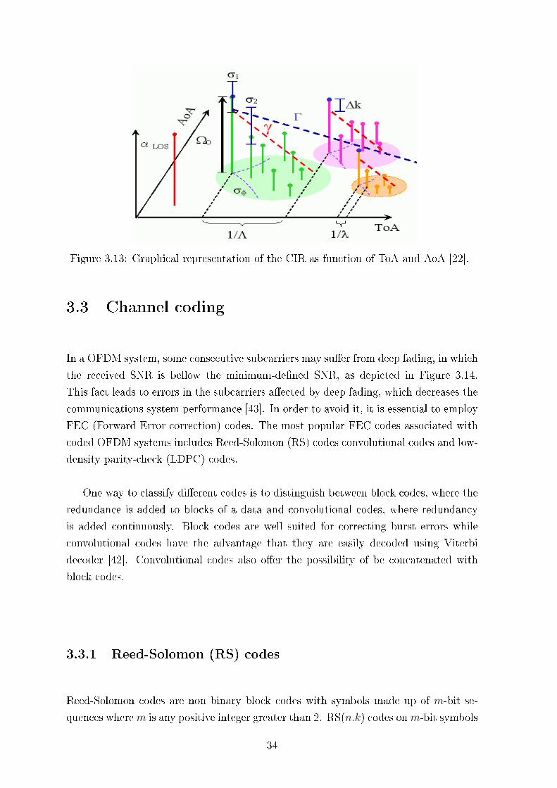
Figure 3.13: Graphical representation of the CIR as function of ToA and AoA [22].
3.3 Channel coding
In a OFDM system, some consecutive subcarriers may suer from deep fading, in which
the received SNR is bellow the minimum-dened SNR, as depicted in Figure 3.14.
This fact leads to errors in the subcarriers aected by deep fading, which decreases the
communications system performance [43]. In order to avoid it, it is essential to employ
FEC (Forward Error correction) codes. The most popular FEC codes associated with
coded OFDM systems includes Reed-Solomon (RS) codes convolutional codes and low-
density parity-check (LDPC) codes.
One way to classify dierent codes is to distinguish between block codes, where the
redundance is added to blocks of a data and convolutional codes, where redundancy
is added continuously. Block codes are well suited for correcting burst errors while
convolutional codes have the advantage that they are easily decoded using Viterbi
decoder [42]. Convolutional codes also oer the possibility of be concatenated with
block codes.
3.3.1 Reed-Solomon (RS) codes
Reed-Solomon codes are non binary block codes with symbols made up of m-bit se-
quences wherem is any positive integer greater than 2. RS(n,k) codes onm-bit symbols
34
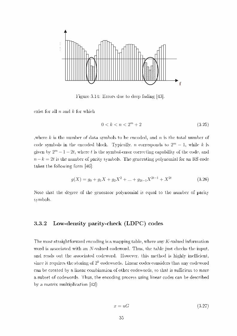
Figure 3.14: Errors due to deep fading [43].
exist for all n and k for which
0 < k < n < 2m + 2 (3.25)
,where k is the number of data symbols to be encoded, and n is the total number of
code symbols in the encoded block. Typically, n corresponds to 2m − 1, while k is
given by 2m− 1− 2t, where t is the symbol-error correcting capability of the code, and
n−k = 2t is the number of parity symbols. The generating polynomial for an RS code
takes the following form [46]:
g(X) = g0 + g1X + g2X2 + ...+ g2t−1X
2t−1 +X2t (3.26)
Note that the degree of the generator polynomial is equal to the number of parity
symbols.
3.3.2 Low-density parity-check (LDPC) codes
The most straightforward encoding is a mapping table, where anyK-valued information
word is associated with an N -valued codeword. Thus, the table just checks the input,
and reads out the associated codeword. However, this method is highly inecient,
since it requires the storing of 2k codewords. Linear codes considers that any codeword
can be created by a linear combination of other codewords, so that is sucient to store
a subset of codewords. Thus, the encoding process using linear codes can be described
by a matrix multiplication [42]:
x = uG (3.27)
35
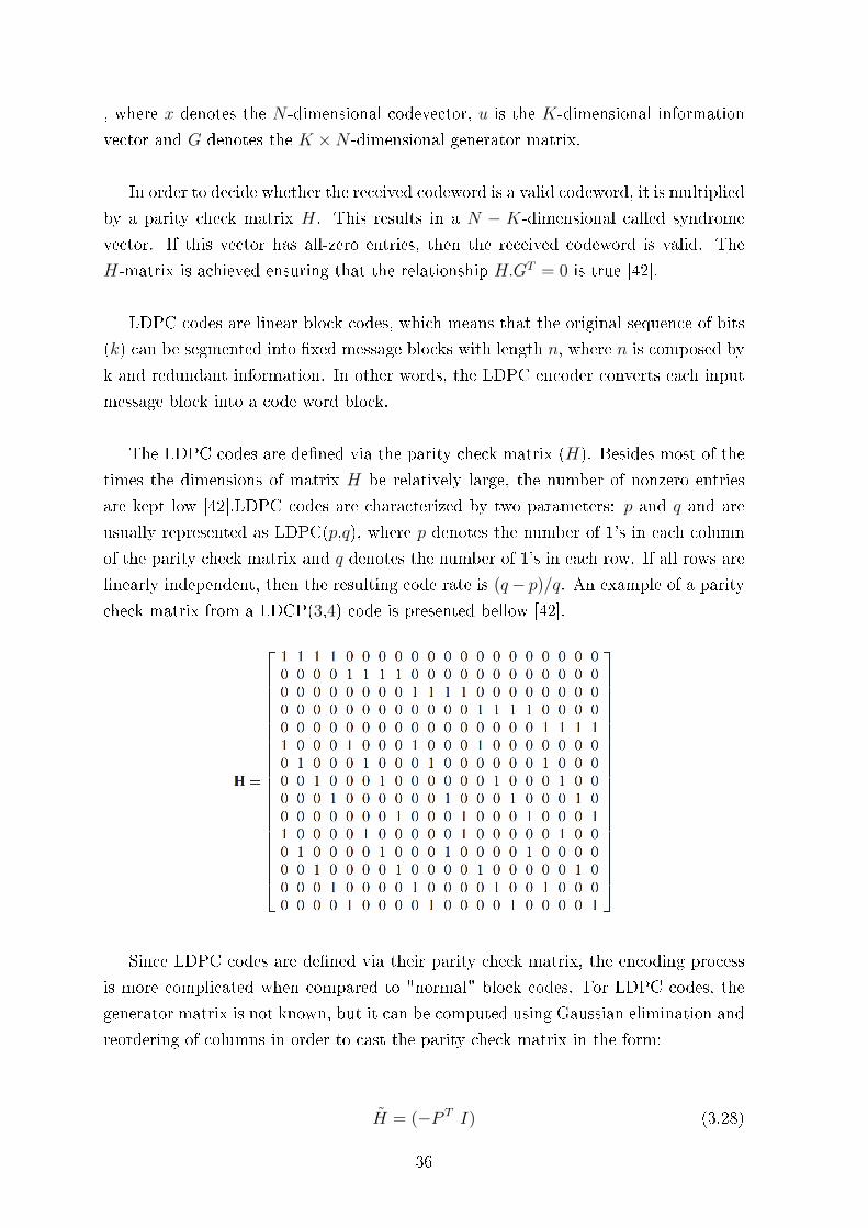
, where x denotes the N -dimensional codevector, u is the K-dimensional information
vector and G denotes the K ×N -dimensional generator matrix.
In order to decide whether the received codeword is a valid codeword, it is multiplied
by a parity check matrix H. This results in a N − K-dimensional called syndrome
vector. If this vector has all-zero entries, then the received codeword is valid. The
H-matrix is achieved ensuring that the relationship H.GT = 0 is true [42].
LDPC codes are linear block codes, which means that the original sequence of bits
(k) can be segmented into xed message blocks with length n, where n is composed by
k and redundant information. In other words, the LDPC encoder converts each input
message block into a code word block.
The LDPC codes are dened via the parity check matrix (H). Besides most of the
times the dimensions of matrix H be relatively large, the number of nonzero entries
are kept low [42].LDPC codes are characterized by two parameters: p and q and are
usually represented as LDPC(p,q), where p denotes the number of 1's in each column
of the parity check matrix and q denotes the number of 1's in each row. If all rows are
linearly independent, then the resulting code rate is (q− p)/q. An example of a parity
check matrix from a LDCP(3,4) code is presented bellow [42].
Since LDPC codes are dened via their parity check matrix, the encoding process
is more complicated when compared to "normal" block codes. For LDPC codes, the
generator matrix is not known, but it can be computed using Gaussian elimination and
reordering of columns in order to cast the parity check matrix in the form:
H = (−P T I) (3.28)
36
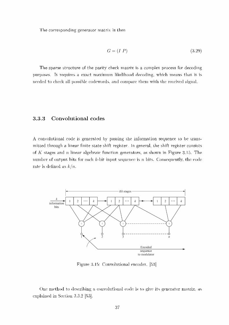
The corresponding generator matrix is then
G = (I P ) (3.29)
The sparse structure of the parity check matrix is a complex process for decoding
purposes. It requires a exact maximum likelihood decoding, which means that it is
needed to check all possible codewords, and compare them with the received signal.
3.3.3 Convolutional codes
A convolutional code is generated by passing the information sequence to be trans-
mitted through a linear nite-state shift register. In general, the shift register consists
of K stages and n linear algebraic function generators, as shown in Figure 3.15. The
number of output bits for each k-bit input sequence is n bits. Consequently, the code
rate is dened as k/n.
Figure 3.15: Convolutional encoder. [53]
One method to describing a convolutional code is to give its generator matrix, as
explained in Section 3.3.2 [53].
37
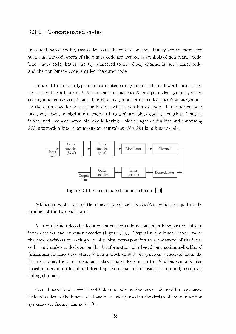
3.3.4 Concatenated codes
In concatenated coding two codes, one binary and one non binary are concatenated
such that the codewords of the binary code are treated as symbols of non binary code.
The binary code that is directly connected to the binary channel is called inner code,
and the non binary code is called the outer code.
Figure 3.16 shows a typical concatenated cdingscheme. The codewords are formed
by subdividing a block of k K information bits into K groups, called symbols, where
each symbol consists of k bits. The K k-bit symbols are encoded into N k-bit symbols
by the outer encoder, as is usually done with a non binary code. The inner encoder
takes each k-bit symbol and encodes it into a binary block code of length n. Thus, it
is obtained a concatenated block code having a block length of Nn bits and containing
kK information bits. that means an equivalent (Nn, kk) long binary code.
Figure 3.16: Concatenated coding scheme. [53]
Additionally, the rate of the concatenated code is Kk/Nn, which is equal to the
product of the two code rates.
A hard decision decoder for a concatenated code is conveniently separated into an
inner decoder and an outer decoder (Figure 3.16). Typically, the inner decoder takes
the hard decisions on each group of n bits, corresponding to a codeword of the inner
code, and makes a decision on the k information bits based on maximum-likelihood
(minimum distance) decoding. When a block of N k-bit symbols is received from the
inner decoder, the outer decoder makes a hard decision on the K k-bit symbols, also
based on maximum-likelihood decoding. Note that soft decision is commonly used over
fading channels.
Concatenated codes with Reed-Solomon codes as the outer code and binary convo-
lutional codes as the inner code have been widely used in the design of communication
systems over fading channels [53].
38
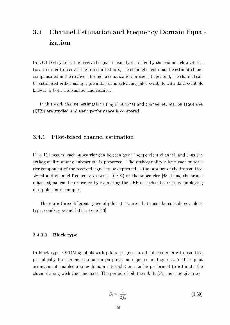
3.4 Channel Estimation and Frequency Domain Equal-
ization
In a OFDM system, the received signal is usually distorted by the channel characteris-
tics. In order to recover the transmitted bits, the channel eect must be estimated and
compensated in the receiver through a equalization process. In general, the channel can
be estimated either using a preamble or interleaving pilot symbols with data symbols
known to both transmitter and receiver.
In this work channel estimation using pilot tones and channel estimation sequences
(CES) are studied and their performance is compared.
3.4.1 Pilot-based channel estimation
If no ICI occurs, each subcarrier can be seen as an independent channel, and thus the
orthogonality among subcarriers is preserved. The orthogonality allows each subcar-
rier component of the received signal to be expressed as the product of the transmitted
signal and channel frequency response (CFR) at the subcarrier [43].Thus, the trans-
mitted signal can be recovered by estimating the CFR at each subcarrier by employing
interpolation techniques.
There are three dierent types of pilot structures that must be considered: block
type, comb type and lattice type [43].
3.4.1.1 Block type
In block type, OFDM symbols with pilots assigned at all subcarriers are transmitted
periodically for channel estimation purposes, as depicted in Figure 3.17 .This pilot
arrangement enables a time-domain interpolation can be performed to estimate the
channel along with the time axis. The period of pilot symbols (St) must be given by
St ≤1
2fd(3.30)
39
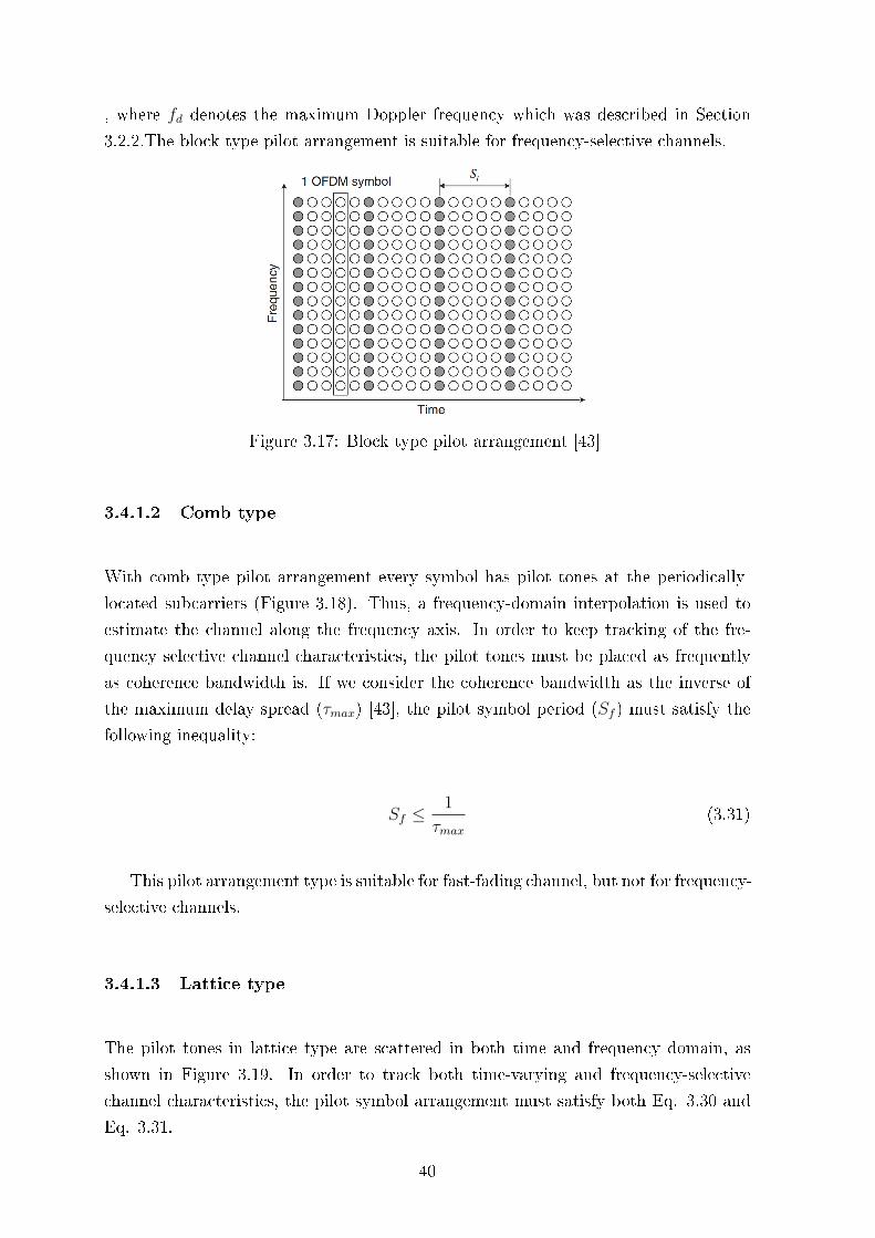
, where fd denotes the maximum Doppler frequency which was described in Section
3.2.2.The block type pilot arrangement is suitable for frequency-selective channels.
Figure 3.17: Block type pilot arrangement [43]
3.4.1.2 Comb type
With comb type pilot arrangement every symbol has pilot tones at the periodically-
located subcarriers (Figure 3.18). Thus, a frequency-domain interpolation is used to
estimate the channel along the frequency axis. In order to keep tracking of the fre-
quency selective channel characteristics, the pilot tones must be placed as frequently
as coherence bandwidth is. If we consider the coherence bandwidth as the inverse of
the maximum delay spread (τmax) [43], the pilot symbol period (Sf ) must satisfy the
following inequality:
Sf ≤1
τmax(3.31)
This pilot arrangement type is suitable for fast-fading channel, but not for frequency-
selective channels.
3.4.1.3 Lattice type
The pilot tones in lattice type are scattered in both time and frequency domain, as
shown in Figure 3.19. In order to track both time-varying and frequency-selective
channel characteristics, the pilot symbol arrangement must satisfy both Eq. 3.30 and
Eq. 3.31.
40
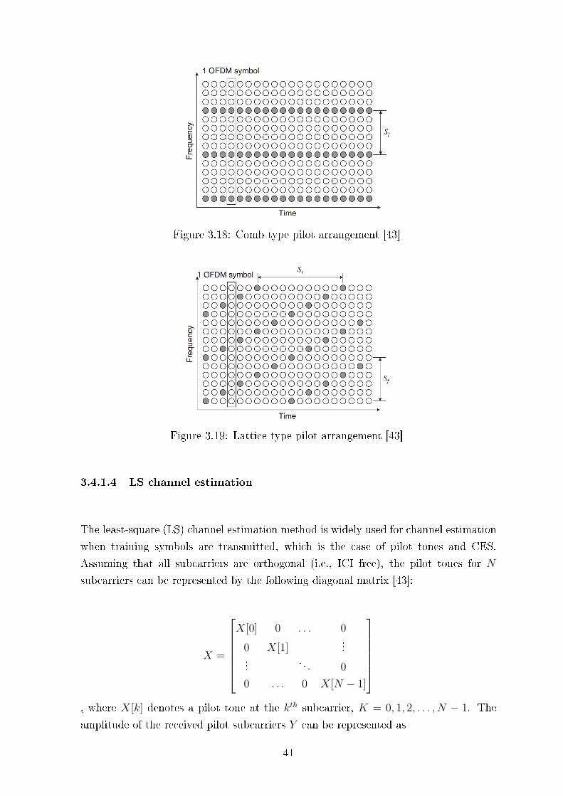
Figure 3.18: Comb type pilot arrangement [43]
Figure 3.19: Lattice type pilot arrangement [43]
3.4.1.4 LS channel estimation
The least-square (LS) channel estimation method is widely used for channel estimation
when training symbols are transmitted, which is the case of pilot tones and CES.
Assuming that all subcarriers are orthogonal (i.e., ICI free), the pilot tones for N
subcarriers can be represented by the following diagonal matrix [43]:
X =
X[0] 0 . . . 0
0 X[1]...
.... . . 0
0 . . . 0 X[N − 1]
, where X[k] denotes a pilot tone at the kth subcarrier, K = 0, 1, 2, . . . , N − 1. The
amplitude of the received pilot subcarriers Y can be represented as
41
Y = XH + Z ⇔
⇔
Y [0]
Y [1]...
Y [N − 1]
=
X[0] 0 . . . 0
0 X[1]...
.... . . 0
0 . . . 0 X[N − 1]
H[0]
H[1]...
H[N − 1]
+
Z[0]
Z[1]...
Z[N − 1]
(3.32)
, where H is the channel vector, and Z represents the noise vector.
The LS estimator nds the channel estimate H in a way that the cost function
(3.33) is minimized as shown in (3.34)
J(H) = ||Y −XH||2
= (Y −XH)∗(Y −XH)
= Y ∗Y − Y ∗XH − H∗X∗Y + H∗X∗XH
(3.33)
, where ∗ denote the complex conjugate.
∂(J(H))
∂(H)= 0 (3.34)
From (3.34) it is obtained the following equality:
X∗XH = X∗Y (3.35)
which gives the solution for the LS channel estimation as stated in [43], [54]
HLS = (X∗X)−1X∗Y = X−1Y (3.36)
This channel estimation technique is a more appropriated approach in terms of low
computational requirements, compared with other methods [55] [56].
42
3.4.1.5 Interpolation techniques
In comb-type pilot-based channel estimation the amplitude of data symbols between
pilot subcarriers must be estimated in order to have a fully estimated frequency re-
sponse of a transmission channel. For that, interpolation techniques are applied to the
estimated pilot subcarriers. Popular interpolation methods include linear interpolation,
second order interpolation, and cubic spline interpolation [43].
According to [57] ,the channel estimation at the data subcarrier k using linear
interpolation is given by Eq.3.37.
H(k) = H(mL+ n)
= [HLS(m+ 1)− HLS(m)]n
L+ HLS(m)
(3.37)
where mL < k < (m+ 1)L and 0 ≤ n < L and m = 0, 1, . . . , Np− 1, where Np denotes
the number of pilot subcarriers. Note that in this equation only two pilots are used for
channel estimation at the data subcarriers.
Second order interpolation performs better than the linear interpolation, since the
channel estimation at the data subcarriers is calculated by using a linear combination
of three adjacent pilots [58]. The channel estimation of second order interpolation is
given by
H(k) = H(mL+ n)
= c1HLS(m− 1) + c0HLS(m) + c−1HLS(m+ 1)(3.38)
,where
c1 = α(α−1)2
,
c0 = −(α− 1)(α + 1),
c−1 = α(α+1)2
,
α = lN
(3.39)
Cubic spline interpolation method allows a smooth and continuous polynomial tted
[58] which is given by:
43
H(k) = H(mL+ n)
= α1HLS(m+ 1) + α0HLS(m) + Lα1H ′LS(m+ 1)− Lα0H ′LS(m)(3.40)
, where H ′LS(m) is the rst order derivative of HLS(m), and
α1 = 3(L−l)2L2 − 2(L−l)3
L3 ,
α0 = 3l2
L2 − 2l3
L3
(3.41)
3.4.2 Golay Complementary Sequences
Golay complementary sequences (GCS) are widely used in the preamble of OFDM and
SC systems for synchronization and as channel estimation sequences (CES) for channel
estimation purposes [7]. Golay sequences are pair of sequences which has an attractive
property that the sum of their auto-correlations has maximum peak with zero side-
lobes [59, 7], which allows to remove ISI in order to improve the accuracy of channel
estimation. Let aN and bN be the pairs of Golay sequences of length equal to N = 2M
(M natural number) and [Ra, Rb] the auto-correlation of each pair respectively, where
the sum both auto-correlations is dened by
Rab(i) = Ra(i) +Rb(i) = 2Nδ(i) (3.42)
Ra(i) =N−i−1∑n=0
aN(n+ i)× a∗N(n) (3.43)
Rb(i) =N−i−1∑n=0
bN(n+ i)× b∗N(n) (3.44)
,where i ∈ [0, ..., N − 1] and δ(i) denotes the Kronecker delta function.
Golay sequences are generated by delay and weigth vectors and a recursive algo-
rithm, as shown in Figure 3.20
44
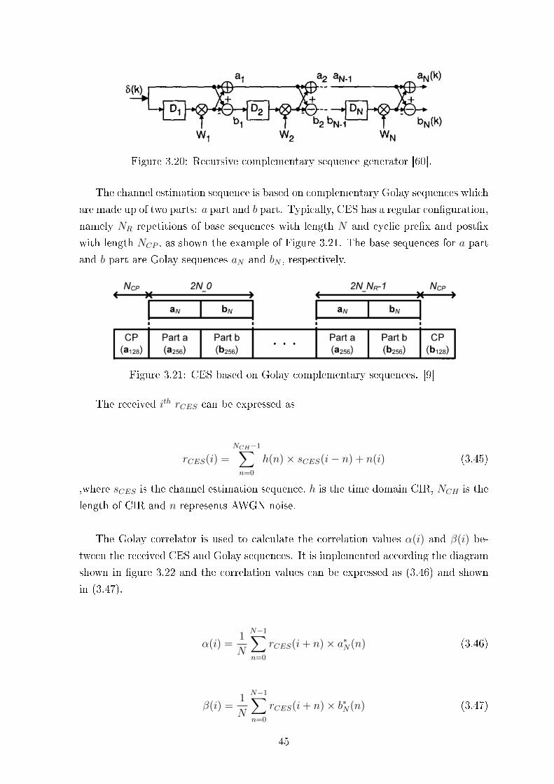
Figure 3.20: Recursive complementary sequence generator [60].
The channel estimation sequence is based on complementary Golay sequences which
are made up of two parts: a part and b part. Typically, CES has a regular conguration,
namely NR repetitions of base sequences with length N and cyclic prex and postx
with length NCP , as shown the example of Figure 3.21. The base sequences for a part
and b part are Golay sequences aN and bN , respectively.
Figure 3.21: CES based on Golay complementary sequences. [9]
The received ith rCES can be expressed as
rCES(i) =
NCH−1∑n=0
h(n)× sCES(i− n) + n(i) (3.45)
,where sCES is the channel estimation sequence, h is the time domain CIR, NCH is the
length of CIR and n represents AWGN noise.
The Golay correlator is used to calculate the correlation values α(i) and β(i) be-
tween the received CES and Golay sequences. It is implemented according the diagram
shown in gure 3.22 and the correlation values can be expressed as (3.46) and shown
in (3.47).
α(i) =1
N
N−1∑n=0
rCES(i+ n)× a∗N(n) (3.46)
β(i) =1
N
N−1∑n=0
rCES(i+ n)× b∗N(n) (3.47)
45
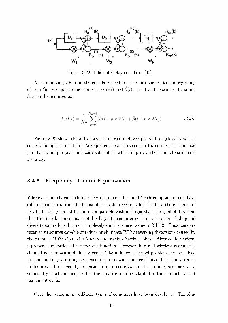
Figure 3.22: Ecient Golay correlator [60].
After removing CP from the correlation values, they are aligned to the beginning
of each Golay sequence and denoted as α(i) and β(i). Finally, the estimated channel
hest can be acquired as
hest(i) =1
NR
NR−1∑p=0
(α(i+ p× 2N) + β(i+ p× 2N)) (3.48)
Figure 3.23 shows the auto correlation results of two parts of length 256 and the
corresponding sum result [7]. As expected, it can be seen that the sum of the sequences
pair has a unique peak and zero side lobes, which improves the channel estimation
accuracy.
3.4.3 Frequency Domain Equalization
Wireless channels can exhibit delay dispersion, i.e. multipath components can have
dierent runtimes from the transmitter to the receiver which leads to the existence of
ISI. If the delay spread becomes comparable with or larger than the symbol duration,
then the BER becomes unacceptably large if no countermeasures are taken. Coding and
diversity can reduce, but not completely eliminate, errors due to ISI [42]. Equalizers are
receiver structures capable of reduce or eliminate ISI by reversing distortions caused by
the channel. If the channel is known and static a hardware-based lter could perform
a proper equalization of the transfer function. However, in a real wireless system, the
channel is unknown and time variant. The unknown channel problem can be solved
by transmitting a training sequence, i.e. a known sequence of bits. The time variance
problem can be solved by repeating the transmission of the training sequence at a
suciently short cadence, so that the equalizer can be adapted to the channel state at
regular intervals.
Over the years, many dierent types of equalizers have been developed. The sim-
46
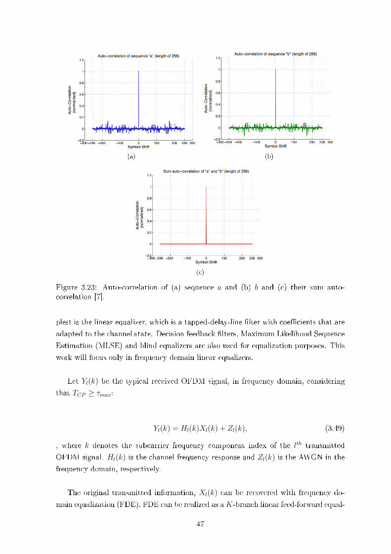
(a) (b)
(c)
Figure 3.23: Auto-correlation of (a) sequence a and (b) b and (c) their sum auto-correlation [7].
plest is the linear equalizer, which is a tapped-delay-line lter with coecients that are
adapted to the channel state. Decision feedback lters, Maximum Likelihood Sequence
Estimation (MLSE) and blind equalizers are also used for equalization purposes. This
work will focus only in frequency domain linear equalizers.
Let Yl(k) be the typical received OFDM signal, in frequency domain, considering
that TCP ≥ τmax:
Yl(k) = Hl(k)Xl(k) + Zl(k), (3.49)
, where k denotes the subcarrier frequency component index of the lth transmitted
OFDM signal. Hl(k) is the channel frequency response and Zl(k) is the AWGN in the
frequency domain, respectively.
The original transmitted information, Xl(k) can be recovered with frequency do-
main equalization (FDE). FDE can be realized as aK-branch linear feed-forward equal-
47
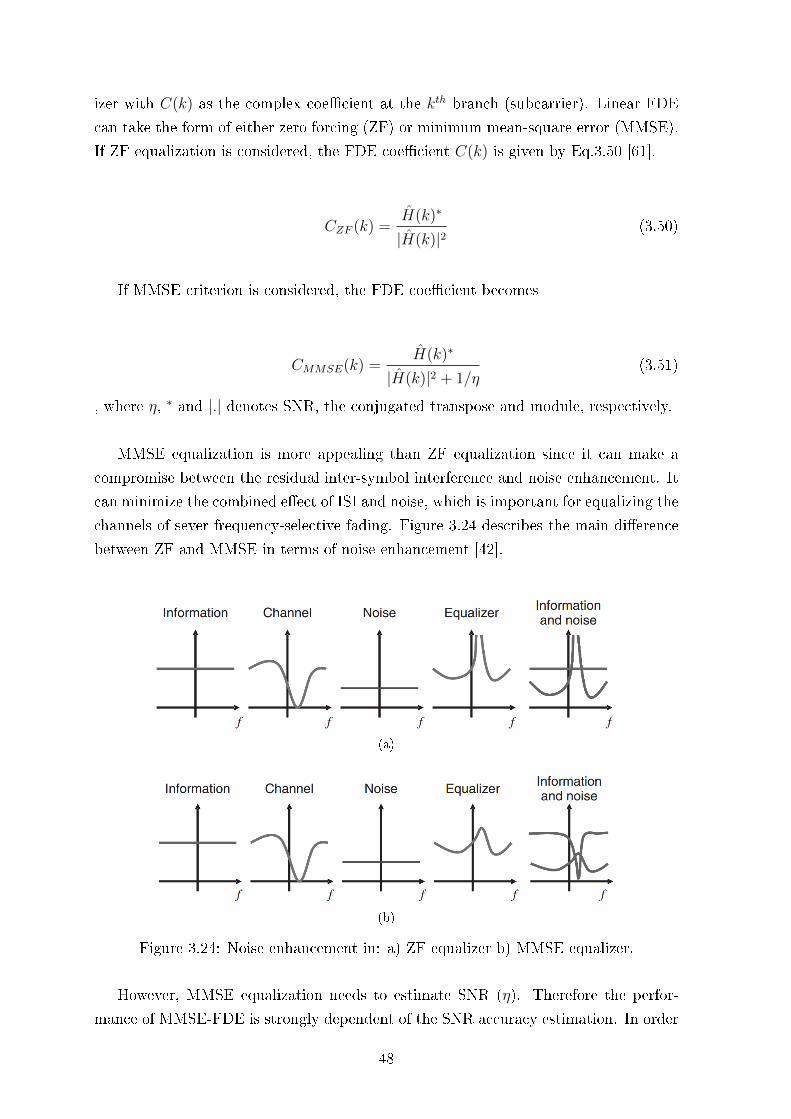
izer with C(k) as the complex coecient at the kth branch (subcarrier). Linear FDE
can take the form of either zero forcing (ZF) or minimum mean-square error (MMSE).
If ZF equalization is considered, the FDE coecient C(k) is given by Eq.3.50 [61].
CZF (k) =H(k)∗
|H(k)|2(3.50)
If MMSE criterion is considered, the FDE coecient becomes
CMMSE(k) =H(k)∗
|H(k)|2 + 1/η(3.51)
, where η, ∗ and |.| denotes SNR, the conjugated transpose and module, respectively.
MMSE equalization is more appealing than ZF equalization since it can make a
compromise between the residual inter-symbol interference and noise enhancement. It
can minimize the combined eect of ISI and noise, which is important for equalizing the
channels of sever frequency-selective fading. Figure 3.24 describes the main dierence
between ZF and MMSE in terms of noise enhancement [42].
(a)
(b)
Figure 3.24: Noise enhancement in: a) ZF equalizer b) MMSE equalizer.
However, MMSE equalization needs to estimate SNR (η). Therefore the perfor-
mance of MMSE-FDE is strongly dependent of the SNR accuracy estimation. In order
48
to estimate SNR, both signal power and noise power must be estimated. According to
[61] the signal power can be estimated as
Ps =1
MK
M∑m=1
|H(k)|2 (3.52)
and the noise power can estimated as
Pn =1
MK
M∑m=1
K∑k=1
|W (m, k)|2 (3.53)
,where W (m, k) = H(k)− H(m, k), m is the index of the channel estimation sequence
received and K is the FFT length.
Finally, the estimated SNR becomes
η =PsPn
(3.54)
Substituting η into (3.51), MMSE FDE coecients results in the following equation:
CMMSE(k) =H(k)∗
|H(k)|2 + 1/η(3.55)
3.5 Summary
Chapter 3 presented an overview of the theoretical fundamentals considered for the
presented work. The rst section gives a short description of OFDM concepts as a
multicarrier scheme for high data rate applications. Section 3.2 introduces the concepts
related to multipath fading channels. The fading channel is subdivided in large-scale
fading eects and small-scale fading eects and the parameters used to characterize
this two categories of fading channel response are detailed. In Section 3.3, the most
commonly used channel coding approaches are presented and the basic analytic expres-
sions are drawn. Finally, the theoretical aspects of channel estimation based on both
49

pilot subcarriers and Golay sequences and frequency domain equalization are discussed
in Section 3.4.
50
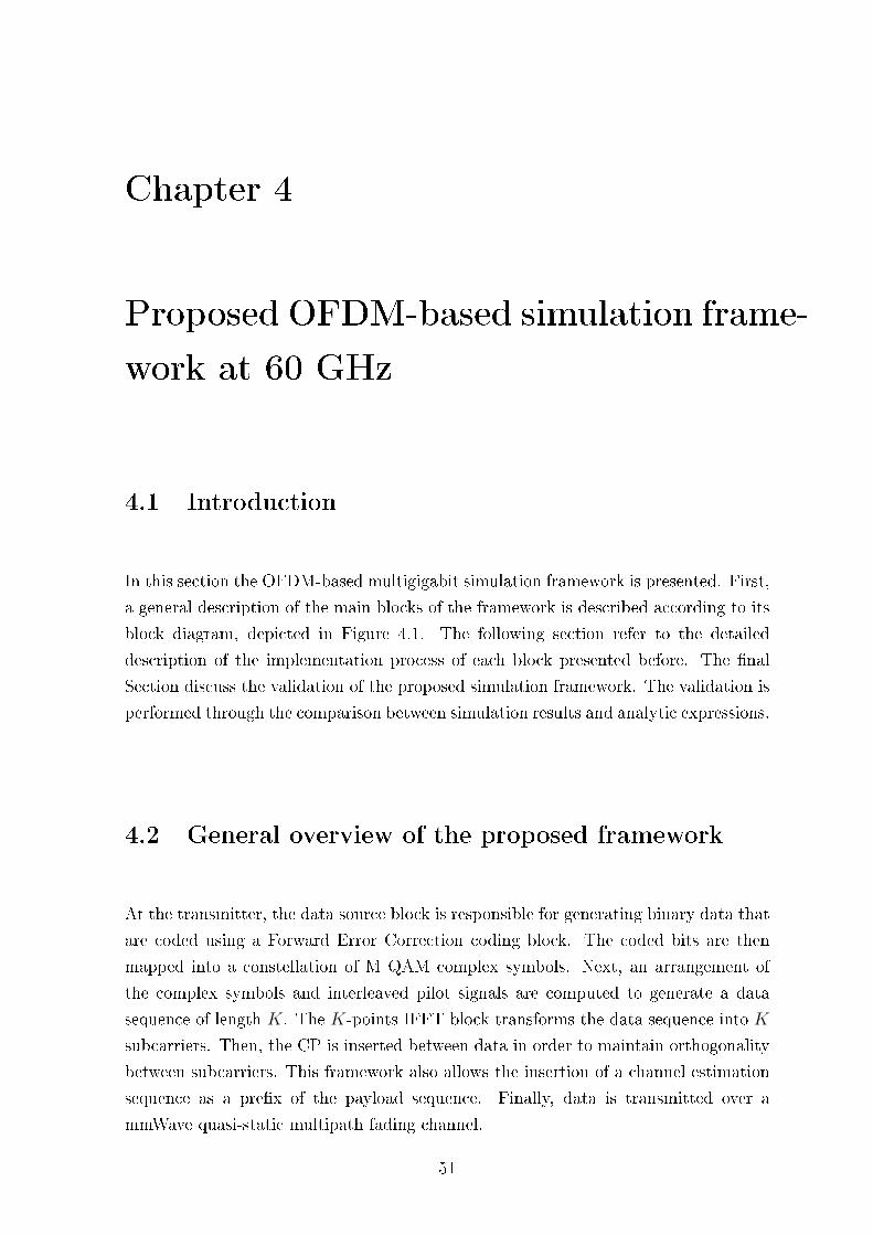
Chapter 4
Proposed OFDM-based simulation frame-
work at 60 GHz
4.1 Introduction
In this section the OFDM-based multigigabit simulation framework is presented. First,
a general description of the main blocks of the framework is described according to its
block diagram, depicted in Figure 4.1. The following section refer to the detailed
description of the implementation process of each block presented before. The nal
Section discuss the validation of the proposed simulation framework. The validation is
performed through the comparison between simulation results and analytic expressions.
4.2 General overview of the proposed framework
At the transmitter, the data source block is responsible for generating binary data that
are coded using a Forward Error Correction coding block. The coded bits are then
mapped into a constellation of M QAM complex symbols. Next, an arrangement of
the complex symbols and interleaved pilot signals are computed to generate a data
sequence of length K. The K-points IFFT block transforms the data sequence into K
subcarriers. Then, the CP is inserted between data in order to maintain orthogonality
between subcarriers. This framework also allows the insertion of a channel estimation
sequence as a prex of the payload sequence. Finally, data is transmitted over a
mmWave quasi-static multipath fading channel.
51
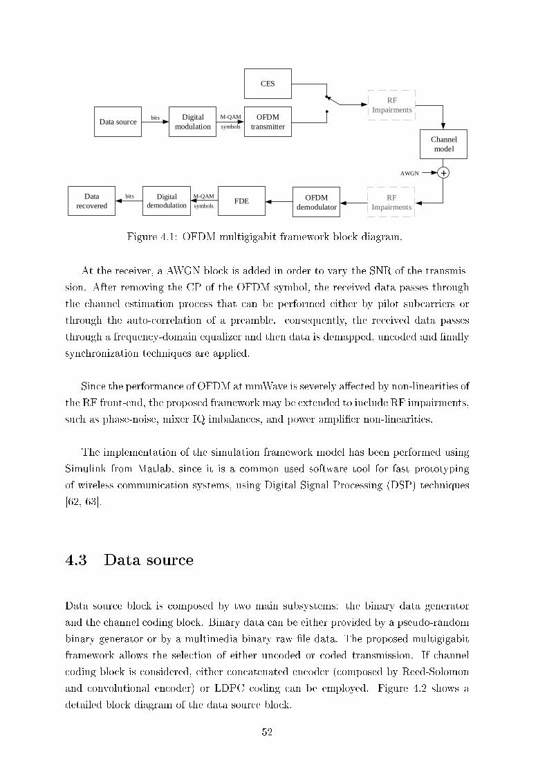
Data sourcebits Digital
modulation
OFDM
transmitter
Channel
model
OFDM
demodulatorFDE
Digital
demodulation
Data
recovered
bits M-QAM
symbols
M-QAM
symbols
AWGN
CES
RF
Impairments
RF
Impairments
+
Figure 4.1: OFDM multigigabit framework block diagram.
At the receiver, a AWGN block is added in order to vary the SNR of the transmis-
sion. After removing the CP of the OFDM symbol, the received data passes through
the channel estimation process that can be performed either by pilot subcarriers or
through the auto-correlation of a preamble. consequently, the received data passes
through a frequency-domain equalizer and then data is demapped, uncoded and nally
synchronization techniques are applied.
Since the performance of OFDM at mmWave is severely aected by non-linearities of
the RF front-end, the proposed framework may be extended to include RF impairments,
such as phase-noise, mixer IQ imbalances, and power amplier non-linearities.
The implementation of the simulation framework model has been performed using
Simulink from Matlab, since it is a common used software tool for fast prototyping
of wireless communication systems, using Digital Signal Processing (DSP) techniques
[62, 63].
4.3 Data source
Data source block is composed by two main subsystems: the binary data generator
and the channel coding block. Binary data can be either provided by a pseudo-random
binary generator or by a multimedia binary raw le data. The proposed multigigabit
framework allows the selection of either uncoded or coded transmission. If channel
coding block is considered, either concatenated encoder (composed by Reed-Solomon
and convolutional encoder) or LDPC coding can be employed. Figure 4.2 shows a
detailed block diagram of the data source block.
52
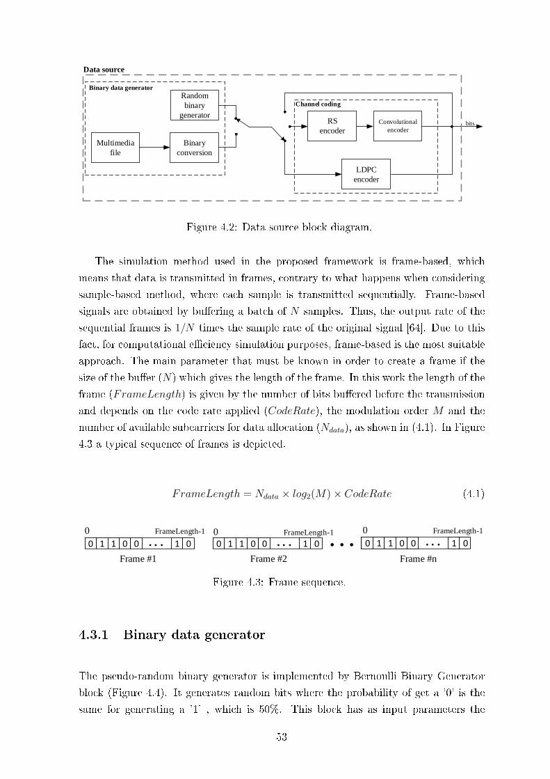
Random
binary
generator
Multimedia
file
Binary
conversion
RS
encoder
LDPC
encoder
bits
Data source
Convolutional
encoder
Channel coding
Binary data generator
Figure 4.2: Data source block diagram.
The simulation method used in the proposed framework is frame-based, which
means that data is transmitted in frames, contrary to what happens when considering
sample-based method, where each sample is transmitted sequentially. Frame-based
signals are obtained by buering a batch of N samples. Thus, the output rate of the
sequential frames is 1/N times the sample rate of the original signal [64]. Due to this
fact, for computational eciency simulation purposes, frame-based is the most suitable
approach. The main parameter that must be known in order to create a frame if the
size of the buer (N) which gives the length of the frame. In this work the length of the
frame (FrameLength) is given by the number of bits buered before the transmission
and depends on the code rate applied (CodeRate), the modulation order M and the
number of available subcarriers for data allocation (Ndata), as shown in (4.1). In Figure
4.3 a typical sequence of frames is depicted.
FrameLength = Ndata × log2(M)× CodeRate (4.1)
0 FrameLength-1
0 1 1 0 010 . . . . . .0 1 1 0 010 . . . 0 1 1 0 010 . . .
Frame #1 Frame #2 Frame #n
0 FrameLength-1 0 FrameLength-1
Figure 4.3: Frame sequence.
4.3.1 Binary data generator
The pseudo-random binary generator is implemented by Bernoulli Binary Generator
block (Figure 4.4). It generates random bits where the probability of get a '0' is the
same for generating a '1' , which is 50%. This block has as input parameters the
53
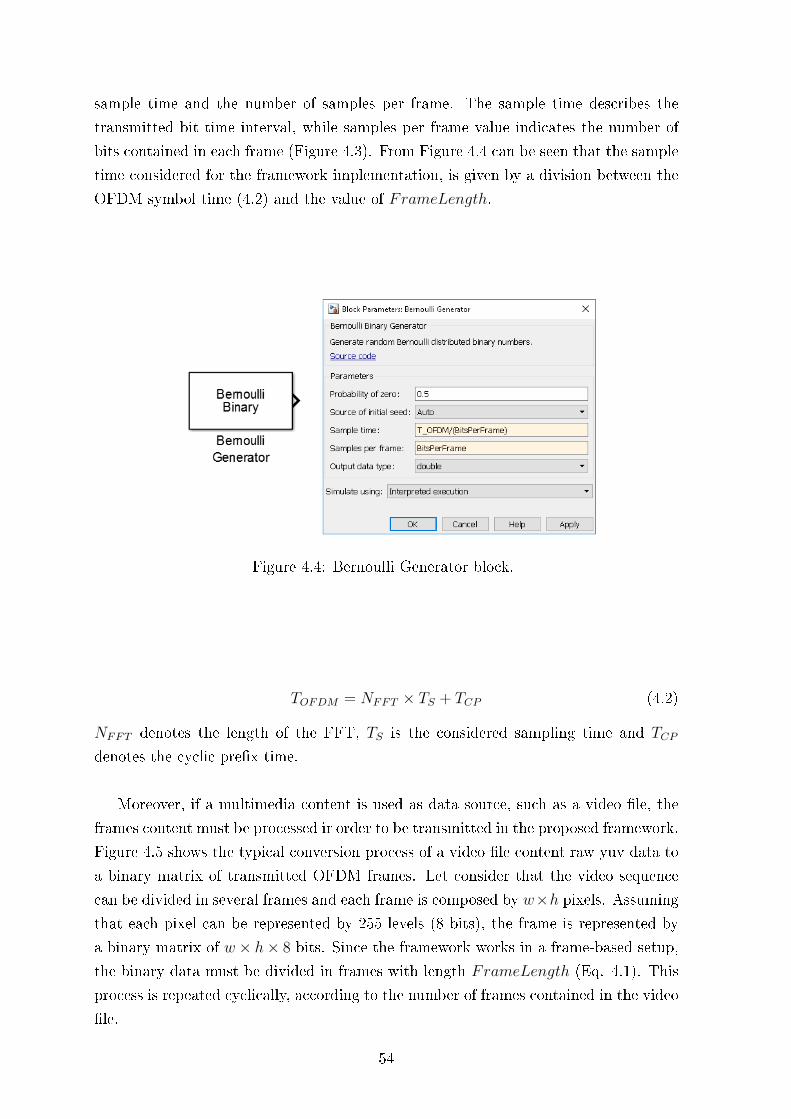
sample time and the number of samples per frame. The sample time describes the
transmitted bit time interval, while samples per frame value indicates the number of
bits contained in each frame (Figure 4.3). From Figure 4.4 can be seen that the sample
time considered for the framework implementation, is given by a division between the
OFDM symbol time (4.2) and the value of FrameLength.
Figure 4.4: Bernoulli Generator block.
TOFDM = NFFT × TS + TCP (4.2)
NFFT denotes the length of the FFT, TS is the considered sampling time and TCP
denotes the cyclic prex time.
Moreover, if a multimedia content is used as data source, such as a video le, the
frames content must be processed ir order to be transmitted in the proposed framework.
Figure 4.5 shows the typical conversion process of a video le content raw yuv data to
a binary matrix of transmitted OFDM frames. Let consider that the video sequence
can be divided in several frames and each frame is composed by w×h pixels. Assuming
that each pixel can be represented by 255 levels (8 bits), the frame is represented by
a binary matrix of w × h× 8 bits. Since the framework works in a frame-based setup,
the binary data must be divided in frames with length FrameLength (Eq. 4.1). This
process is repeated cyclically, according to the number of frames contained in the video
le.
54
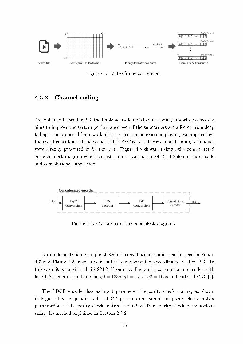
0 w-1
0 w x h x 8 -1
0 1 1 0 010 . . .
0
h-1
0 BitsPerFrame-1
0 1 1 0 010 . . .
0 BitsPerFrame-1
0 1 1 0 010 . . .
0 BitsPerFrame-1
0 1 1 0 010 . . .
. . .
Video file w x h pixeis video frame Binary-format video frame Frames to be transmitted
Figure 4.5: Video frame conversion.
4.3.2 Channel coding
As explained in Section 3.3, the implementation of channel coding in a wireless system
aims to improve the system performance even if the subcarriers are aected from deep
fading. The proposed framework allows coded transmission employing two approaches:
the use of concatenated codes and LDCP FEC codes. These channel coding techniques
were already presented in Section 3.3. Figure 4.6 shows in detail the concatenated
encoder block diagram which consists in a concatenation of Reed-Solomon outer code
and convolutional inner code.
bits
Concatenated encoder
Byte
conversion
RS
encoder
Bit
conversion
Convolutional
encoder
bits
Figure 4.6: Concatenated encoder block diagram.
An implementation example of RS and convolutional coding can be seen in Figure
4.7 and Figure 4.8, respectively and it is implemented according to Section 3.3. In
this case, it is considered RS(224,216) outer coding and a convolutional encoder with
length 7, generator polynomial g0 = 133o, g1 = 171o, g2 = 165o and code rate 2/3 [2].
The LDCP encoder has as input parameter the parity check matrix, as shown
in Figure 4.9. Appendix A.4 and C.4 presents an example of parity check matrix
permutations. The parity check matrix is obtained from parity check permutations
using the method explained in Section 2.3.2.
55
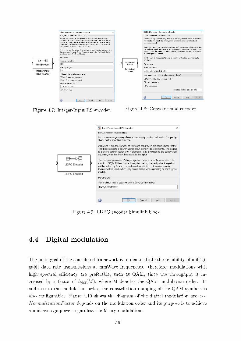
Figure 4.7: Integer-Input RS encoder. Figure 4.8: Convolutional encoder.
Figure 4.9: LDPC encoder Simulink block.
4.4 Digital modulation
The main goal of the considered framework is to demonstrate the reliability of miltigi-
gabit data rate transmissions at mmWave frequencies. therefore, modulations with
high spectral eciency are preferable, such as QAM, since the throughput is in-
creased by a factor of log2(M), where M denotes the QAM modulation order. In
addition to the modulation order, the constellation mapping of the QAM symbols is
also congurable. Figure 4.10 shows the diagram of the digital modulation process.
NormalizationFactor depends on the modulation order and its purpose is to achieve
a unit average power regardless the M-ary modulation.
56
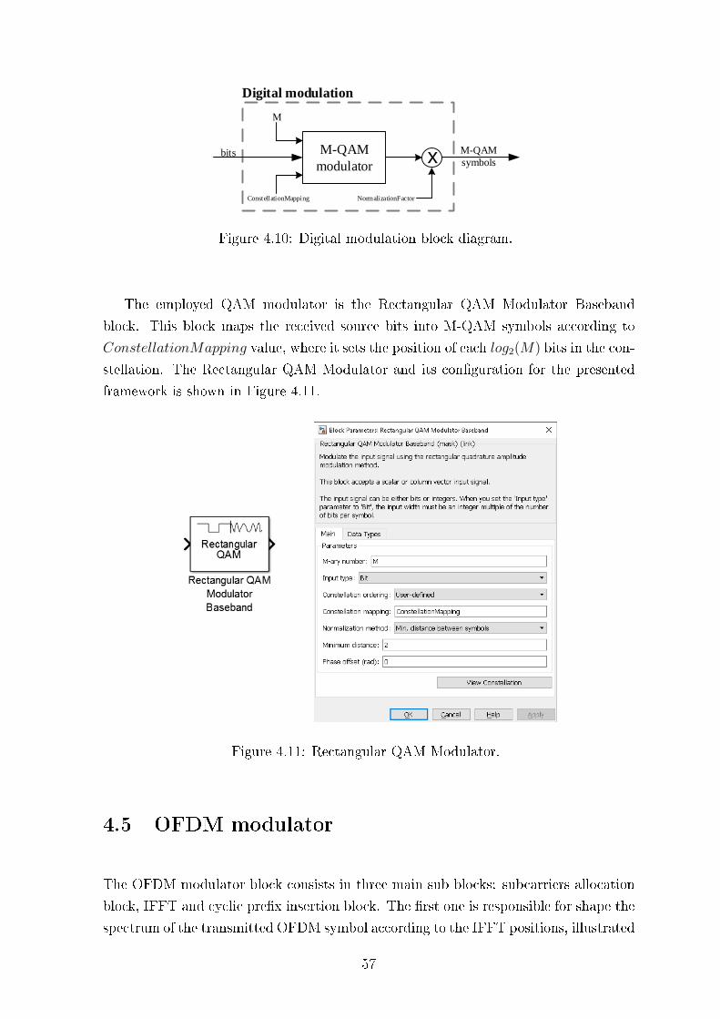
M-QAM
modulator
M-QAM
Digital modulation
symbols
M
ConstellationMapping
bits
NormalizationFactor
x
Figure 4.10: Digital modulation block diagram.
The employed QAM modulator is the Rectangular QAM Modulator Baseband
block. This block maps the received source bits into M-QAM symbols according to
ConstellationMapping value, where it sets the position of each log2(M) bits in the con-
stellation. The Rectangular QAM Modulator and its conguration for the presented
framework is shown in Figure 4.11.
Figure 4.11: Rectangular QAM Modulator.
4.5 OFDM modulator
The OFDM modulator block consists in three main sub blocks: subcarriers allocation
block, IFFT and cyclic prex insertion block. The rst one is responsible for shape the
spectrum of the transmitted OFDM symbol according to the IFFT positions, illustrated
57
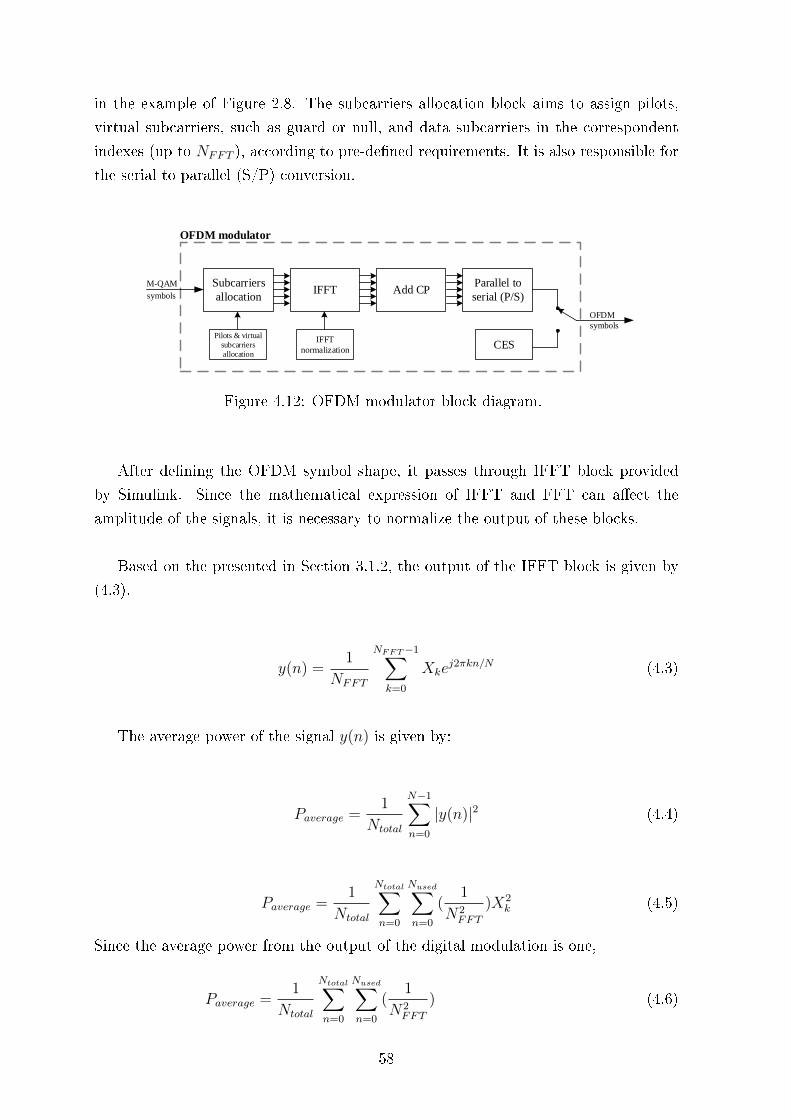
in the example of Figure 2.8. The subcarriers allocation block aims to assign pilots,
virtual subcarriers, such as guard or null, and data subcarriers in the correspondent
indexes (up to NFFT ), according to pre-dened requirements. It is also responsible for
the serial to parallel (S/P) conversion.
Subcarriers
allocation
OFDM modulator
M-QAMIFFT Add CP
Parallel to
serial (P/S)
CESIFFT
normalization
Pilots & virtual
subcarriers
allocation
symbols
OFDM
symbols
Figure 4.12: OFDM modulator block diagram.
After dening the OFDM symbol shape, it passes through IFFT block provided
by Simulink. Since the mathematical expression of IFFT and FFT can aect the
amplitude of the signals, it is necessary to normalize the output of these blocks.
Based on the presented in Section 3.1.2, the output of the IFFT block is given by
(4.3).
y(n) =1
NFFT
NFFT−1∑k=0
Xkej2πkn/N (4.3)
The average power of the signal y(n) is given by:
Paverage =1
Ntotal
N−1∑n=0
|y(n)|2 (4.4)
Paverage =1
Ntotal
Ntotal∑n=0
Nused∑n=0
(1
N2FFT
)X2k (4.5)
Since the average power from the output of the digital modulation is one,
Paverage =1
Ntotal
Ntotal∑n=0
Nused∑n=0
(1
N2FFT
) (4.6)
58
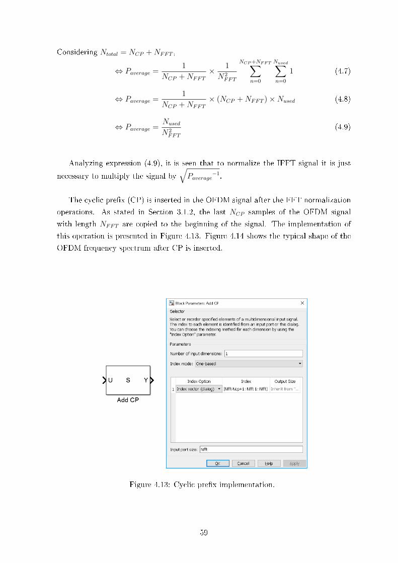
Considering Ntotal = NCP +NFFT ,
⇔ Paverage =1
NCP +NFFT
× 1
N2FFT
NCP +NFFT∑n=0
Nused∑n=0
1 (4.7)
⇔ Paverage =1
NCP +NFFT
× (NCP +NFFT )×Nused (4.8)
⇔ Paverage =Nused
N2FFT
(4.9)
Analyzing expression (4.9), it is seen that to normalize the IFFT signal it is just
necessary to multiply the signal by√Paverage
−1.
The cyclic prex (CP) is inserted in the OFDM signal after the FFT normalization
operations. As stated in Section 3.1.2, the last NCP samples of the OFDM signal
with length NFFT are copied to the beginning of the signal. The implementation of
this operation is presented in Figure 4.13. Figure 4.14 shows the typical shape of the
OFDM frequency spectrum after CP is inserted.
Figure 4.13: Cyclic prex implementation.
59
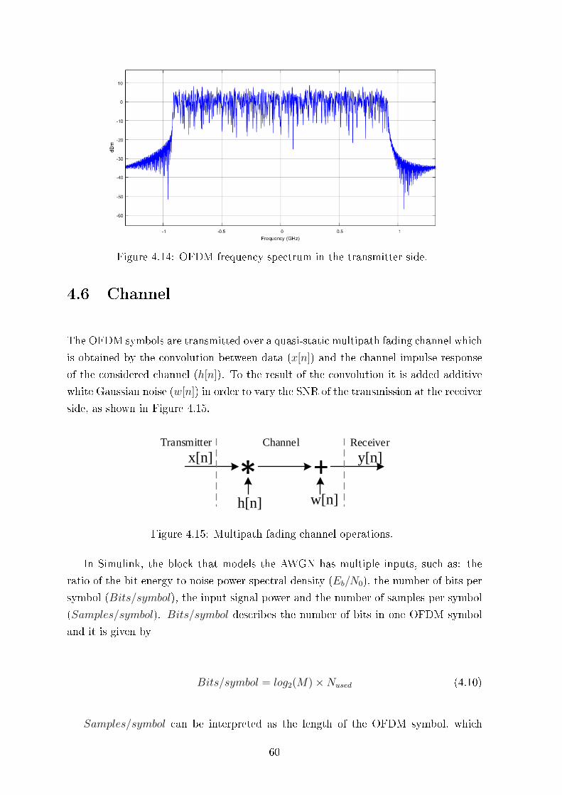
Figure 4.14: OFDM frequency spectrum in the transmitter side.
4.6 Channel
The OFDM symbols are transmitted over a quasi-static multipath fading channel which
is obtained by the convolution between data (x[n]) and the channel impulse response
of the considered channel (h[n]). To the result of the convolution it is added additive
white Gaussian noise (w[n]) in order to vary the SNR of the transmission at the receiver
side, as shown in Figure 4.15.
*x[n]
h[n]
+ y[n]ChannelTransmitter Receiver
w[n]
Figure 4.15: Multipath fading channel operations.
In Simulink, the block that models the AWGN has multiple inputs, such as: the
ratio of the bit energy to noise power spectral density (Eb/N0), the number of bits per
symbol (Bits/symbol), the input signal power and the number of samples per symbol
(Samples/symbol). Bits/symbol describes the number of bits in one OFDM symbol
and it is given by
Bits/symbol = log2(M)×Nused (4.10)
Samples/symbol can be interpreted as the length of the OFDM symbol, which
60
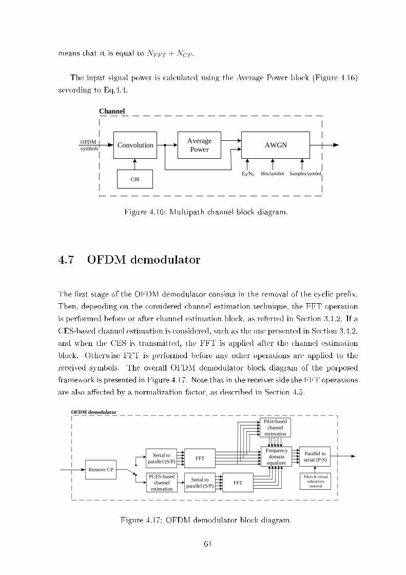
means that it is equal to NFFT +NCP .
The input signal power is calculated using the Average Power block (Figure 4.16)
according to Eq.4.4.
Convolution
Channel
Average
Power
CIR
OFDM
symbolsAWGN
Bits/symbolEb/N0 Samples/symbol
Figure 4.16: Multipath channel block diagram.
4.7 OFDM demodulator
The rst stage of the OFDM demodulator consists in the removal of the cyclic prex.
Then, depending on the considered channel estimation technique, the FFT operation
is performed before or after channel estimation block, as referred in Section 3.1.2. If a
CES-based channel estimation is considered, such as the one presented in Section 3.4.2,
and when the CES is transmitted, the FFT is applied after the channel estimation
block. Otherwise FFT is performed before any other operations are applied to the
received symbols. The overall OFDM demodulator block diagram of the porposed
framework is presented in Figure 4.17. Note that in the receiver side the FFT operations
are also aected by a normalization factor, as described in Section 4.5.
OFDM demodulator
Remove CP
Serial to
parallel (S/P)FFT
Frequency
domain
equalizer
Parallel to
serial (P/S)
Pilot-based
channel
estimation
PCES-based
channel
estimation
Serial to
parallel (S/P)FFT
Pilots & virtual
subcarriers
removal
Figure 4.17: OFDM demodulator block diagram.
61
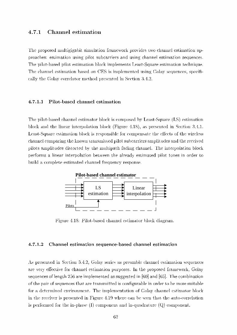
4.7.1 Channel estimation
The proposed multigigabit simulation framework provides two channel estimation ap-
proaches: estimation using pilot subcarriers and using channel estimation sequences.
The pilot-based pilot estimation block implements Least-Square estimation technique.
The channel estimation based on CES is implemented using Golay sequences, speci-
cally the Golay correlator method presented in Section 3.4.2.
4.7.1.1 Pilot-based channel estimation
The pilot-based channel estimator block is composed by Least-Square (LS) estimation
block and the linear interpolation block (Figure 4.18), as presented in Section 3.4.1.
Least-Square estimation block is responsible for compensate the eects of the wireless
channel comparing the known transmitted pilot subcarriers amplitudes and the received
pilots amplitudes distorted by the multipath fading channel. The interpolation block
performs a linear interpolation between the already estimated pilot tones in order to
build a complete estimated channel frequency response.
Pilot-based channel estimator
LS
estimation
Linear
interpolation
Pilots
Figure 4.18: Pilot-based channel estimator block diagram.
4.7.1.2 Channel estimation sequence-based channel estimation
As presented in Section 3.4.2, Golay series as preamble channel estimation sequences
are very eective for channel estimation purposes. In the proposed framework, Golay
sequences of length 256 are implemented as suggested in [60] and [65]. The combination
of the pair of sequences that are transmitted is congurable in order to be more suitable
for a determined environment. The implementation of Golay channel estimator block
in the receiver is presented in Figure 4.19 where can be seen that the auto-correlation
is performed for the in-phase (I) component and in-quadrature (Q) component.
62
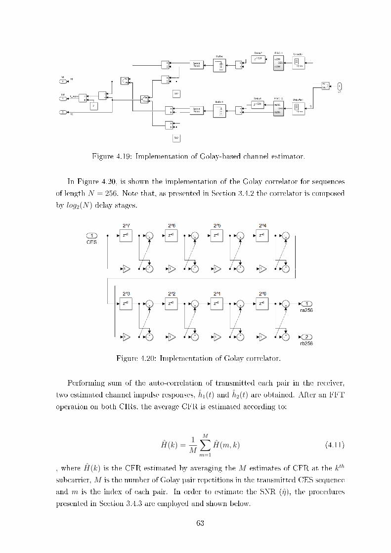
Figure 4.19: Implementation of Golay-based channel estimator.
In Figure 4.20, is shown the implementation of the Golay correlator for sequences
of length N = 256. Note that, as presented in Section 3.4.2 the correlator is composed
by log2(N) delay stages.
Figure 4.20: Implementation of Golay correlator.
Performing sum of the auto-correlation of transmitted each pair in the receiver,
two estimated channel impulse responses, h1(t) and h2(t) are obtained. After an FFT
operation on both CIRs, the average CFR is estimated according to:
H(k) =1
M
M∑m=1
H(m, k) (4.11)
, where H(k) is the CFR estimated by averaging the M estimates of CFR at the kth
subcarrier,M is the number of Golay pair repetitions in the transmitted CES sequence
and m is the index of each pair. In order to estimate the SNR (η), the procedures
presented in Section 3.4.3 are employed and shown below.
63
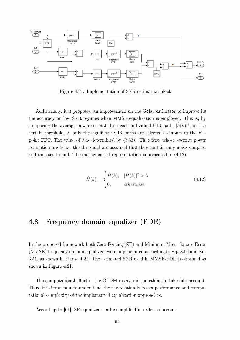
Figure 4.21: Implementation of SNR estimation block.
Additionally, it is proposed an improvement on the Golay estimator to improve its
the accuracy on low SNR regimes when MMSE equalization is employed. This is, by
comparing the average power estimated on each individual CIR path, |h(k)|2, with a
certain threshold, λ, only the signicant CIR paths are selected as inputs to the K -
point FFT. The value of λ is determined by (3.53). Therefore, whose average power
estimation are below the threshold are assumed that they contain only noise samples,
and thus set to null. The mathematical representation is presented in (4.12).
H(k) =
H(k), |H(k)|2 > λ
0, otherwise(4.12)
4.8 Frequency domain equalizer (FDE)
In the proposed framework both Zero Forcing (ZF) and Minimum Mean Square Error
(MMSE) frequency domain equalizers were implemented according to Eq. 3.50 and Eq.
3.51, as shown in Figure 4.22. The estimated SNR used in MMSE-FDE is obtained as
shown in Figure 4.21.
The computational eort in the OFDM receiver is something to take into account.
Thus, it is important to understand the the relation between performance and compu-
tational complexity of the implemented equalization approaches.
According to [61], ZF equalizer can be simplied in order to become
64
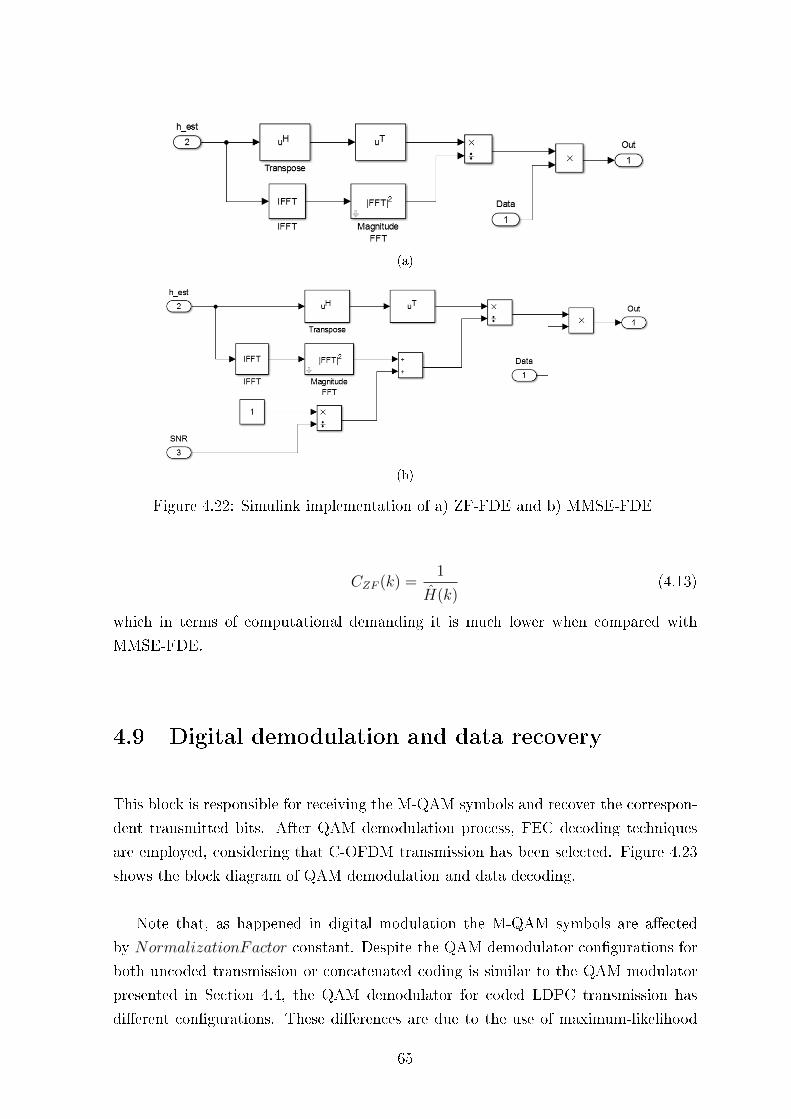
(a)
(b)
Figure 4.22: Simulink implementation of a) ZF-FDE and b) MMSE-FDE
CZF (k) =1
H(k)(4.13)
which in terms of computational demanding it is much lower when compared with
MMSE-FDE.
4.9 Digital demodulation and data recovery
This block is responsible for receiving the M-QAM symbols and recover the correspon-
dent transmitted bits. After QAM demodulation process, FEC decoding techniques
are employed, considering that C-OFDM transmission has been selected. Figure 4.23
shows the block diagram of QAM demodulation and data decoding.
Note that, as happened in digital modulation the M-QAM symbols are aected
by NormalizationFactor constant. Despite the QAM demodulator congurations for
both uncoded transmission or concatenated coding is similar to the QAM modulator
presented in Section 4.4, the QAM demodulator for coded LDPC transmission has
dierent congurations. These dierences are due to the use of maximum-likelihood
65
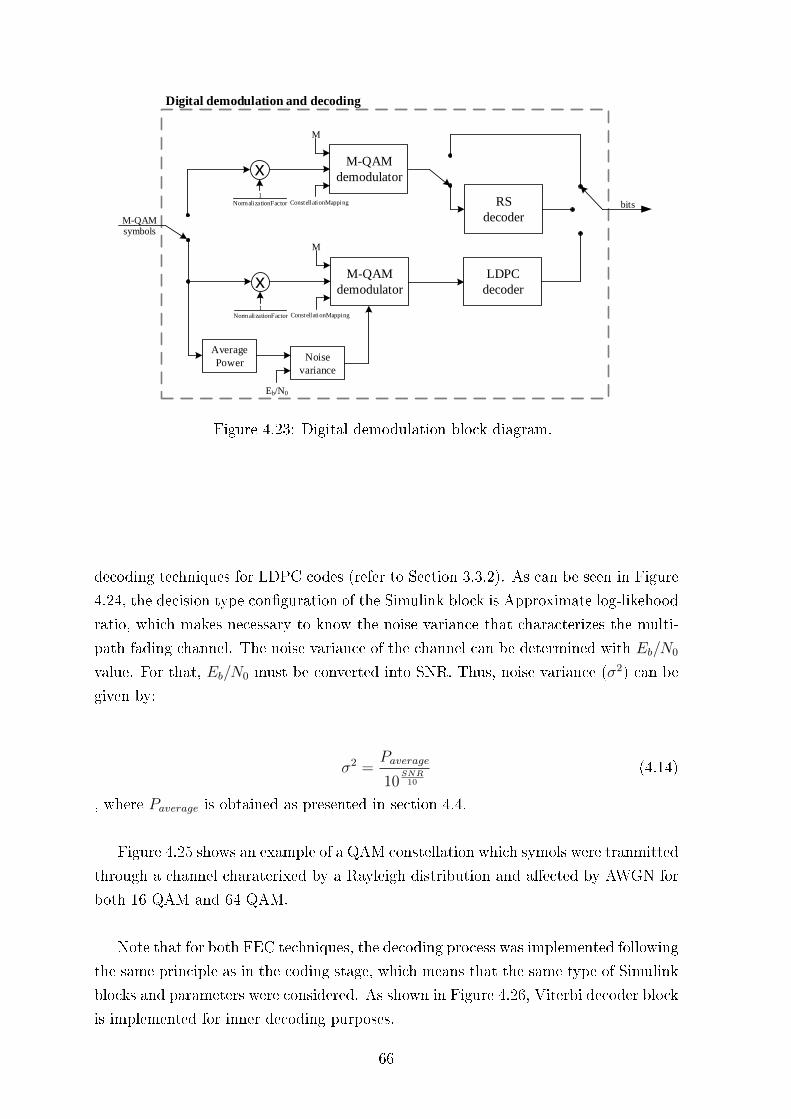
M-QAM
demodulator
Digital demodulation and decoding
M
ConstellationMapping bits1
NormalizationFactor
x
M-QAM
demodulator
M
ConstellationMapping
Eb/N0
1
NormalizationFactor
xLDPC
decoder
RS
decoder
Average
PowerNoise
variance
M-QAMsymbols
Figure 4.23: Digital demodulation block diagram.
decoding techniques for LDPC codes (refer to Section 3.3.2). As can be seen in Figure
4.24, the decision type conguration of the Simulink block is Approximate log-likehood
ratio, which makes necessary to know the noise variance that characterizes the multi-
path fading channel. The noise variance of the channel can be determined with Eb/N0
value. For that, Eb/N0 must be converted into SNR. Thus, noise variance (σ2) can be
given by:
σ2 =Paverage
10SNR10
(4.14)
, where Paverage is obtained as presented in section 4.4.
Figure 4.25 shows an example of a QAM constellation which symols were tranmitted
through a channel charaterixed by a Rayleigh distribution and aected by AWGN for
both 16 QAM and 64 QAM.
Note that for both FEC techniques, the decoding process was implemented following
the same principle as in the coding stage, which means that the same type of Simulink
blocks and parameters were considered. As shown in Figure 4.26, Viterbi decoder block
is implemented for inner decoding purposes.
66
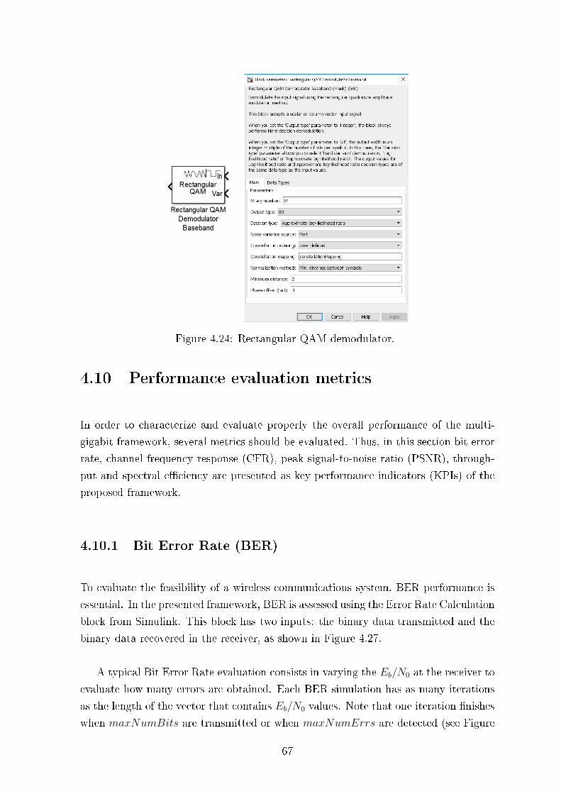
Figure 4.24: Rectangular QAM demodulator.
4.10 Performance evaluation metrics
In order to characterize and evaluate properly the overall performance of the multi-
gigabit framework, several metrics should be evaluated. Thus, in this section bit error
rate, channel frequency response (CFR), peak signal-to-noise ratio (PSNR), through-
put and spectral eciency are presented as key performance indicators (KPIs) of the
proposed framework.
4.10.1 Bit Error Rate (BER)
To evaluate the feasibility of a wireless communications system, BER performance is
essential. In the presented framework, BER is assessed using the Error Rate Calculation
block from Simulink. This block has two inputs: the binary data transmitted and the
binary data recovered in the receiver, as shown in Figure 4.27.
A typical Bit Error Rate evaluation consists in varying the Eb/N0 at the receiver to
evaluate how many errors are obtained. Each BER simulation has as many iterations
as the length of the vector that contains Eb/N0 values. Note that one iteration nishes
when maxNumBits are transmitted or when maxNumErrs are detected (see Figure
67
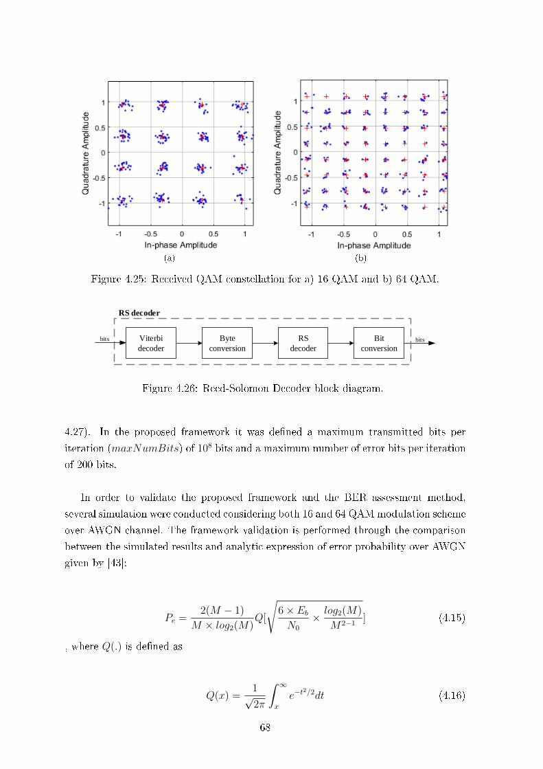
(a) (b)
Figure 4.25: Received QAM constellation for a) 16 QAM and b) 64 QAM.
bits
RS decoder
Byte
conversion
RS
decoder
Bit
conversion
Viterbi
decoder
bits
Figure 4.26: Reed-Solomon Decoder block diagram.
4.27). In the proposed framework it was dened a maximum transmitted bits per
iteration (maxNumBits) of 108 bits and a maximum number of error bits per iteration
of 200 bits.
In order to validate the proposed framework and the BER assessment method,
several simulation were conducted considering both 16 and 64 QAMmodulation scheme
over AWGN channel. The framework validation is performed through the comparison
between the simulated results and analytic expression of error probability over AWGN
given by [43]:
Pe =2(M − 1)
M × log2(M)Q[
√6× EbN0
× log2(M)
M2−1] (4.15)
, where Q(.) is dened as
Q(x) =1√2π
ˆ ∞x
e−t2/2dt (4.16)
68
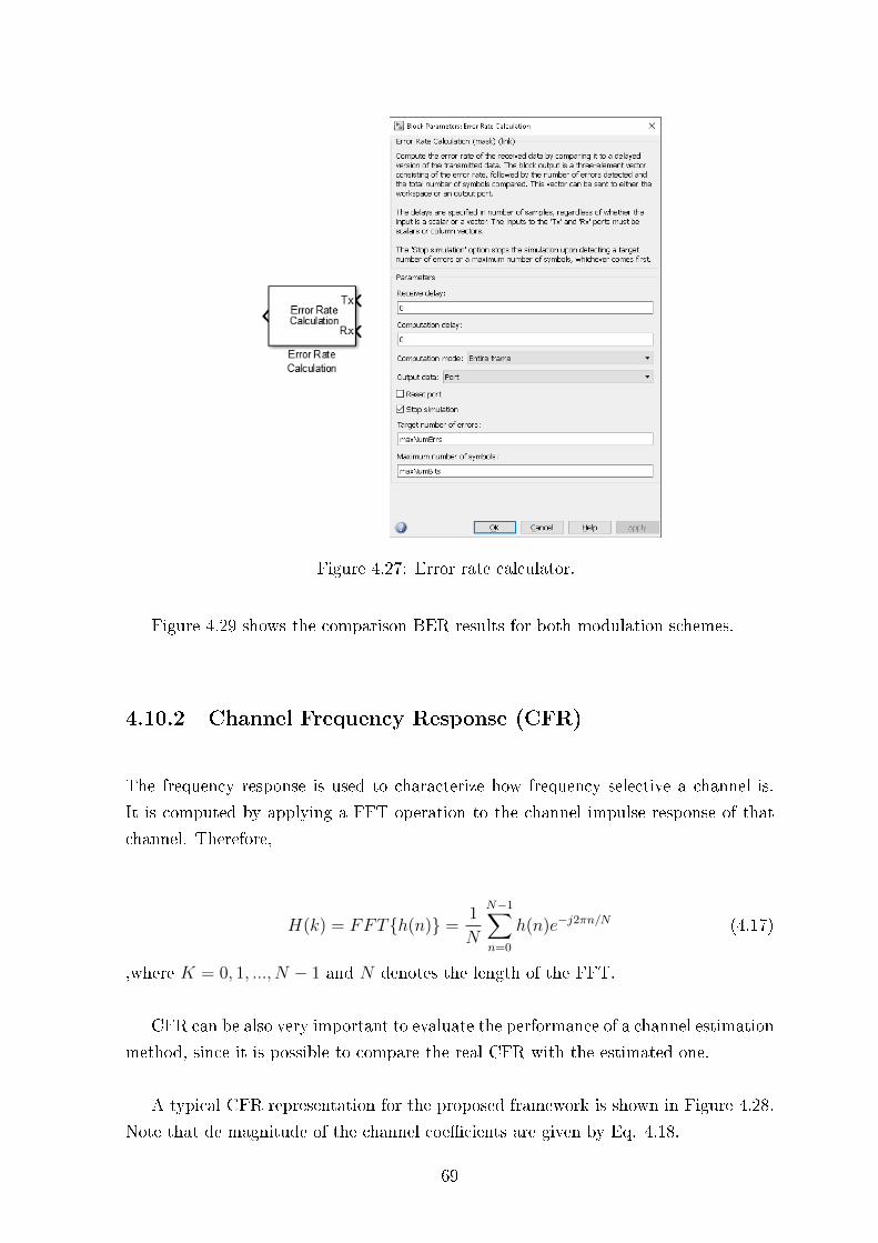
Figure 4.27: Error rate calculator.
Figure 4.29 shows the comparison BER results for both modulation schemes.
4.10.2 Channel Frequency Response (CFR)
The frequency response is used to characterize how frequency selective a channel is.
It is computed by applying a FFT operation to the channel impulse response of that
channel. Therefore,
H(k) = FFTh(n) =1
N
N−1∑n=0
h(n)e−j2πn/N (4.17)
,where K = 0, 1, ..., N − 1 and N denotes the length of the FFT.
CFR can be also very important to evaluate the performance of a channel estimation
method, since it is possible to compare the real CFR with the estimated one.
A typical CFR representation for the proposed framework is shown in Figure 4.28.
Note that de magnitude of the channel coecients are given by Eq. 4.18.
69
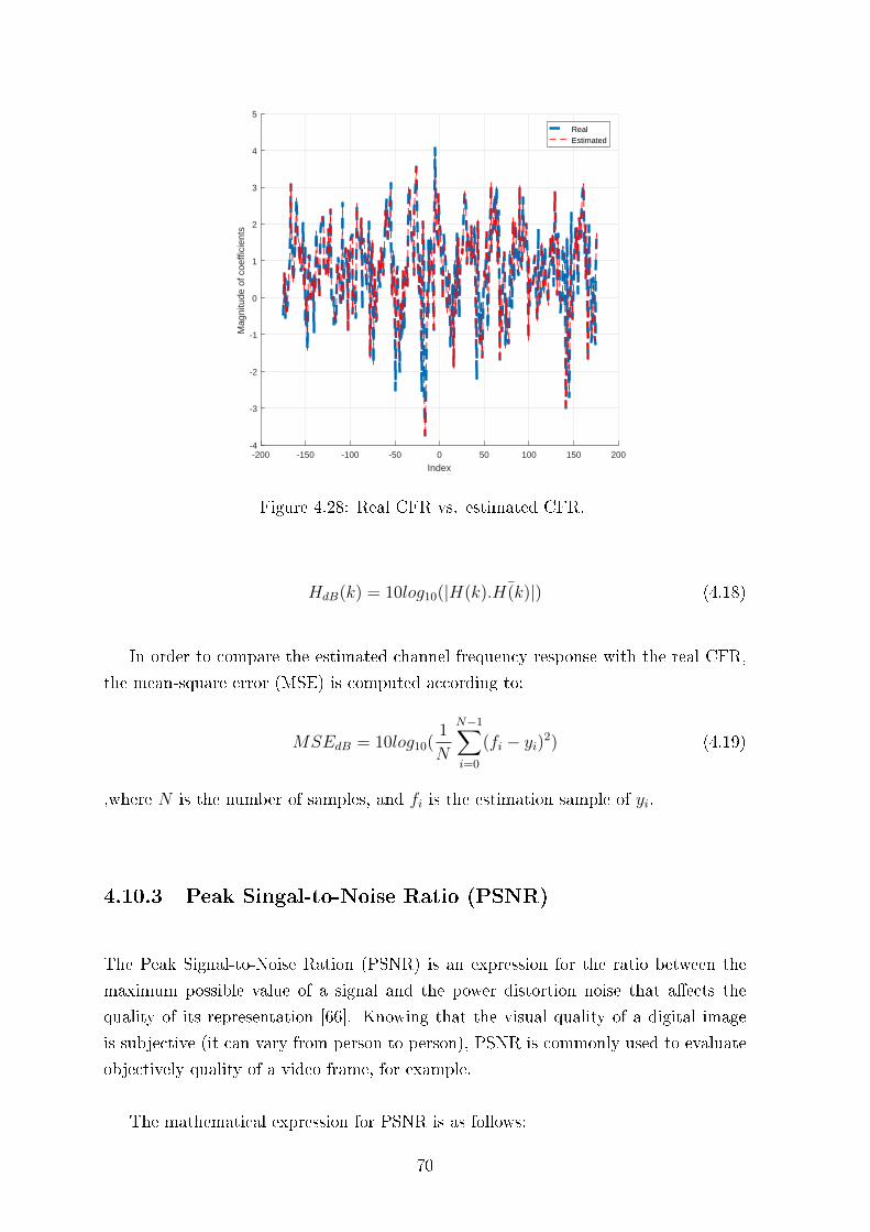
-200 -150 -100 -50 0 50 100 150 200
Index
-4
-3
-2
-1
0
1
2
3
4
5
Mag
nitu
de o
f coe
ffici
ents
RealEstimated
Figure 4.28: Real CFR vs. estimated CFR.
HdB(k) = 10log10(|H(k). ¯H(k)|) (4.18)
In order to compare the estimated channel frequency response with the real CFR,
the mean-square error (MSE) is computed according to:
MSEdB = 10log10(1
N
N−1∑i=0
(fi − yi)2) (4.19)
,where N is the number of samples, and fi is the estimation sample of yi.
4.10.3 Peak Singal-to-Noise Ratio (PSNR)
The Peak Signal-to-Noise Ration (PSNR) is an expression for the ratio between the
maximum possible value of a signal and the power distortion noise that aects the
quality of its representation [66]. Knowing that the visual quality of a digital image
is subjective (it can vary from person to person), PSNR is commonly used to evaluate
objectively quality of a video frame, for example.
The mathematical expression for PSNR is as follows:
70
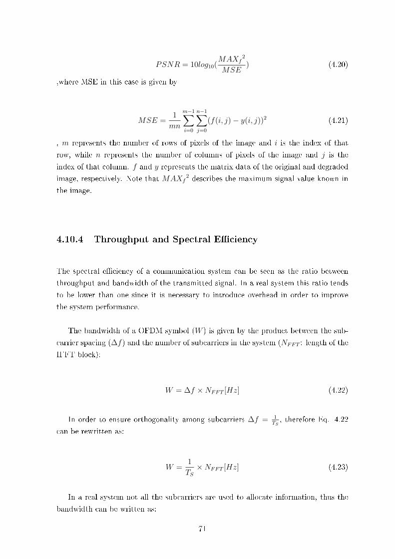
PSNR = 10log10(MAXf
2
MSE) (4.20)
,where MSE in this case is given by
MSE =1
mn
m−1∑i=0
n−1∑j=0
(f(i, j)− y(i, j))2 (4.21)
, m represents the number of rows of pixels of the image and i is the index of that
row, while n represents the number of columns of pixels of the image and j is the
index of that column. f and y represents the matrix data of the original and degraded
image, respectively. Note that MAXf2 describes the maximum signal value known in
the image.
4.10.4 Throughput and Spectral Eciency
The spectral eciency of a communication system can be seen as the ratio between
throughput and bandwidth of the transmitted signal. In a real system this ratio tends
to be lower than one since it is necessary to introduce overhead in order to improve
the system performance.
The bandwidth of a OFDM symbol (W ) is given by the product between the sub-
carrier spacing (∆f) and the number of subcarriers in the system (NFFT : length of the
IFFT block):
W = ∆f ×NFFT [Hz] (4.22)
In order to ensure orthogonality among subcarriers ∆f = 1TS, therefore Eq. 4.22
can be rewritten as:
W =1
TS×NFFT [Hz] (4.23)
In a real system not all the subcarriers are used to allocate information, thus the
bandwidth can be written as:
71
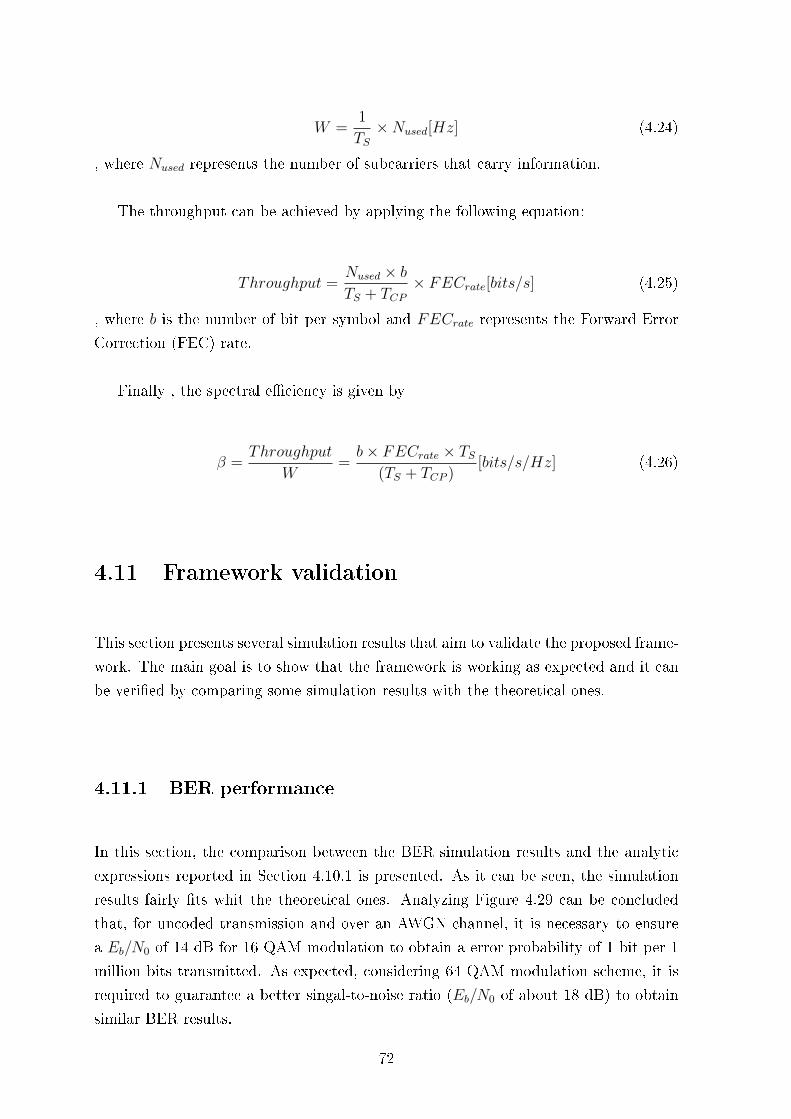
W =1
TS×Nused[Hz] (4.24)
, where Nused represents the number of subcarriers that carry information.
The throughput can be achieved by applying the following equation:
Throughput =Nused × bTS + TCP
× FECrate[bits/s] (4.25)
, where b is the number of bit per symbol and FECrate represents the Forward Error
Correction (FEC) rate.
Finally , the spectral eciency is given by
β =Throughput
W=b× FECrate × TS
(TS + TCP )[bits/s/Hz] (4.26)
4.11 Framework validation
This section presents several simulation results that aim to validate the proposed frame-
work. The main goal is to show that the framework is working as expected and it can
be veried by comparing some simulation results with the theoretical ones.
4.11.1 BER performance
In this section, the comparison between the BER simulation results and the analytic
expressions reported in Section 4.10.1 is presented. As it can be seen, the simulation
results fairly ts whit the theoretical ones. Analyzing Figure 4.29 can be concluded
that, for uncoded transmission and over an AWGN channel, it is necessary to ensure
a Eb/N0 of 14 dB for 16 QAM modulation to obtain a error probability of 1 bit per 1
million bits transmitted. As expected, considering 64 QAM modulation scheme, it is
required to guarantee a better singal-to-noise ratio (Eb/N0 of about 18 dB) to obtain
similar BER results.
72
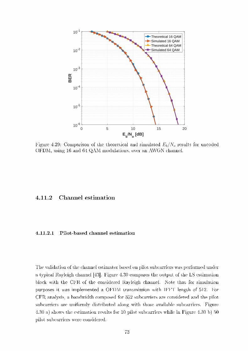
0 5 10 15 20
Eb/N
o [dB]
10-6
10-5
10-4
10-3
10-2
10-1
BE
R
Theoretical 16 QAMSimulated 16 QAMTheoretical 64 QAMSimulated 64 QAM
Figure 4.29: Comparison of the theoretical and simulated Eb/No results for uncodedOFDM, using 16 and 64 QAM modulations, over an AWGN channel.
4.11.2 Channel estimation
4.11.2.1 Pilot-based channel estimation
The validation of the channel estimator based on pilot subcarriers was performed under
a typical Rayleigh channel [43]. Figure 4.30 compares the output of the LS estimation
block with the CFR of the considered Rayleigh channel. Note that for simulation
purposes it was implemented a OFDM transmission with IFFT length of 512. For
CFR analysis, a bandwidth composed for 352 subcarriers are considered and the pilot
subcarriers are uniformly distributed along with those available subcarriers. Figure
4.30 a) shows the estimation results for 10 pilot subcarriers while in Figure 4.30 b) 50
pilot subcarriers were considered.
73
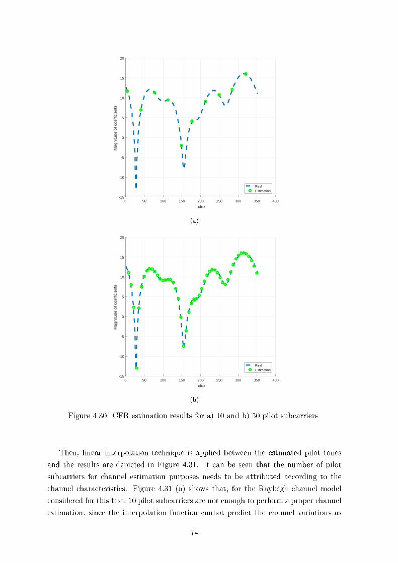
0 50 100 150 200 250 300 350 400
Index
-15
-10
-5
0
5
10
15
20
Mag
nitu
de o
f coe
ffici
ents
RealEstimation
(a)
0 50 100 150 200 250 300 350 400
Index
-15
-10
-5
0
5
10
15
20
Mag
nitu
de o
f coe
ffici
ents
RealEstimation
(b)
Figure 4.30: CFR estimation results for a) 10 and b) 50 pilot subcarriers
Then, linear interpolation technique is applied between the estimated pilot tones
and the results are depicted in Figure 4.31. It can be seen that the number of pilot
subcarriers for channel estimation purposes needs to be attributed according to the
channel characteristics. Figure 4.31 (a) shows that, for the Rayleigh channel model
considered for this test, 10 pilot subcarriers are not enough to perform a proper channel
estimation, since the interpolation function cannot predict the channel variations as
74
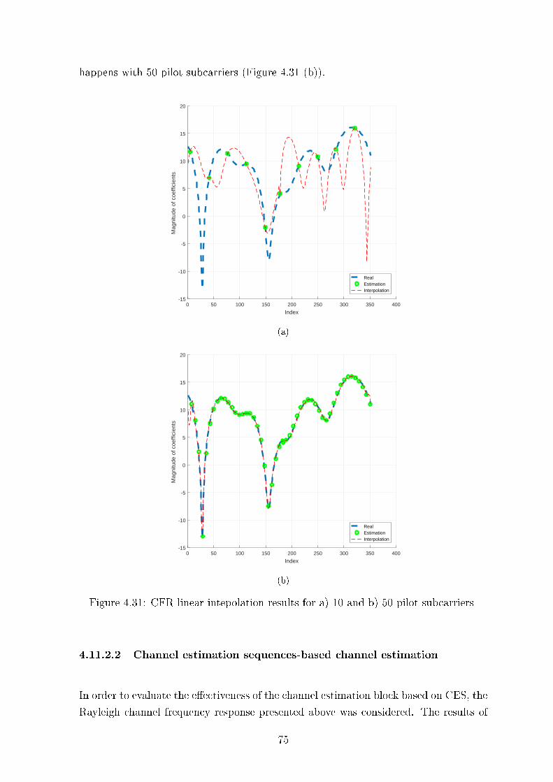
happens with 50 pilot subcarriers (Figure 4.31 (b)).
0 50 100 150 200 250 300 350 400
Index
-15
-10
-5
0
5
10
15
20
Mag
nitu
de o
f coe
ffici
ents
RealEstimationInterpolation
(a)
0 50 100 150 200 250 300 350 400
Index
-15
-10
-5
0
5
10
15
20
Mag
nitu
de o
f coe
ffici
ents
RealEstimationInterpolation
(b)
Figure 4.31: CFR linear intepolation results for a) 10 and b) 50 pilot subcarriers
4.11.2.2 Channel estimation sequences-based channel estimation
In order to evaluate the eectiveness of the channel estimation block based on CES, the
Rayleigh channel frequency response presented above was considered. The results of
75
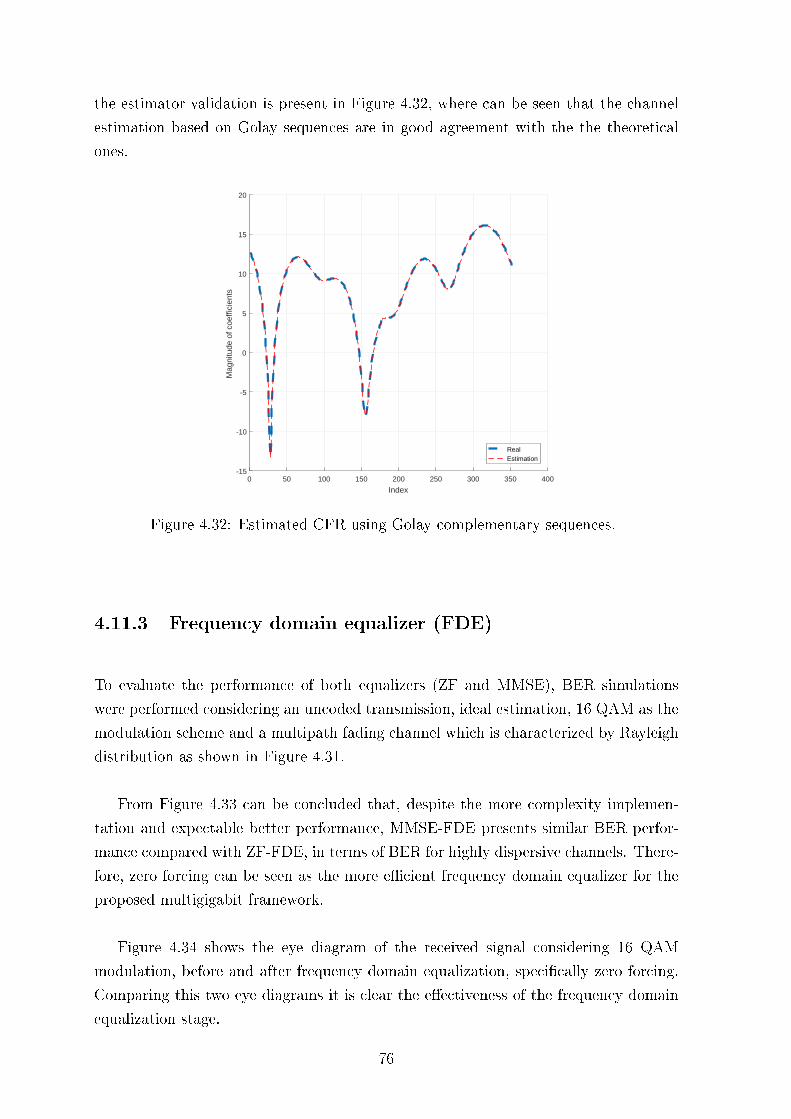
the estimator validation is present in Figure 4.32, where can be seen that the channel
estimation based on Golay sequences are in good agreement with the the theoretical
ones.
0 50 100 150 200 250 300 350 400
Index
-15
-10
-5
0
5
10
15
20
Mag
nitu
de o
f coe
ffici
ents
RealEstimation
Figure 4.32: Estimated CFR using Golay complementary sequences.
4.11.3 Frequency domain equalizer (FDE)
To evaluate the performance of both equalizers (ZF and MMSE), BER simulations
were performed considering an uncoded transmission, ideal estimation, 16 QAM as the
modulation scheme and a multipath fading channel which is characterized by Rayleigh
distribution as shown in Figure 4.31.
From Figure 4.33 can be concluded that, despite the more complexity implemen-
tation and expectable better performance, MMSE-FDE presents similar BER perfor-
mance compared with ZF-FDE, in terms of BER for highly dispersive channels. There-
fore, zero forcing can be seen as the more ecient frequency domain equalizer for the
proposed multigigabit framework.
Figure 4.34 shows the eye diagram of the received signal considering 16 QAM
modulation, before and after frequency domain equalization, specically zero forcing.
Comparing this two eye diagrams it is clear the eectiveness of the frequency domain
equalization stage.
76
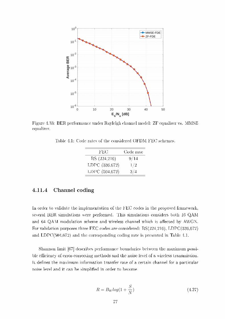
0 10 20 30 40 50
Eb/N
o [dB]
10-6
10-5
10-4
10-3
10-2
10-1
100
Ave
rag
e B
ER
MMSE-FDEZF-FDE
Figure 4.33: BER performance under Rayleigh channel model: ZF equalizer vs. MMSEequalizer.
Table 4.1: Code rates of the considered OFDM FEC schemes.
FEC Code rate
RS (224,216) 9/14
LDPC (336,672) 1/2
LDPC (504,672) 3/4
4.11.4 Channel coding
In order to validate the implementation of the FEC codes in the proposed framework,
several BER simulations were performed. This simulations considers both 16 QAM
and 64 QAM modulation scheme and wireless channel which is aected by AWGN.
For validation purposes three FEC codes are considered: RS(224,216), LDPC(336,672)
and LDPC(504,672) and the corresponding coding rate is presented in Table 4.1.
Shannon limit [67] describes performance boundaries between the maximum possi-
ble eciency of error-correcting methods and the noise level of a wireless transmission.
It denes the maximum information transfer rate of a certain channel for a particular
noise level and it can be simplied in order to become
R = BW log(1 +S
N) (4.27)
77
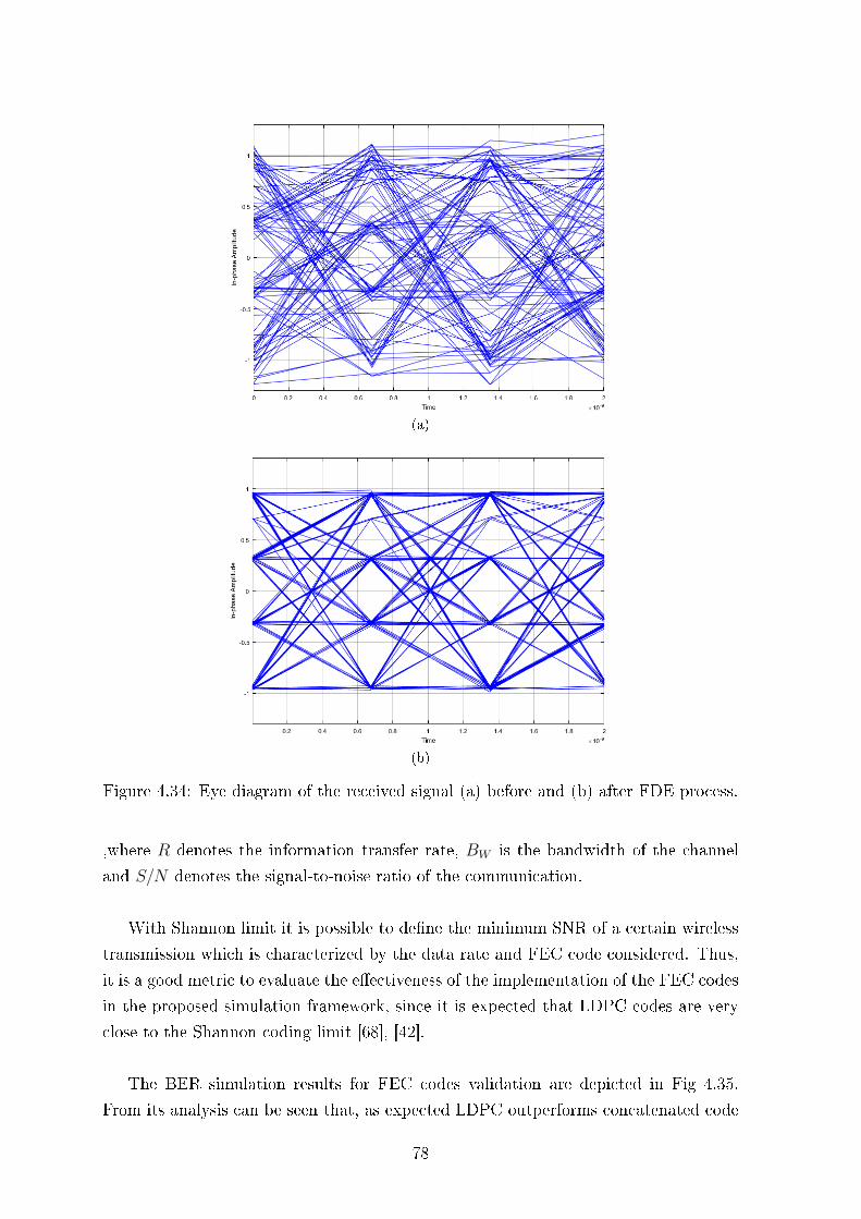
(a)
(b)
Figure 4.34: Eye diagram of the received signal (a) before and (b) after FDE process.
,where R denotes the information transfer rate, BW is the bandwidth of the channel
and S/N denotes the signal-to-noise ratio of the communication.
With Shannon limit it is possible to dene the minimum SNR of a certain wireless
transmission which is characterized by the data rate and FEC code considered. Thus,
it is a good metric to evaluate the eectiveness of the implementation of the FEC codes
in the proposed simulation framework, since it is expected that LDPC codes are very
close to the Shannon coding limit [68], [42].
The BER simulation results for FEC codes validation are depicted in Fig 4.35.
From its analysis can be seen that, as expected LDPC outperforms concatenated code
78
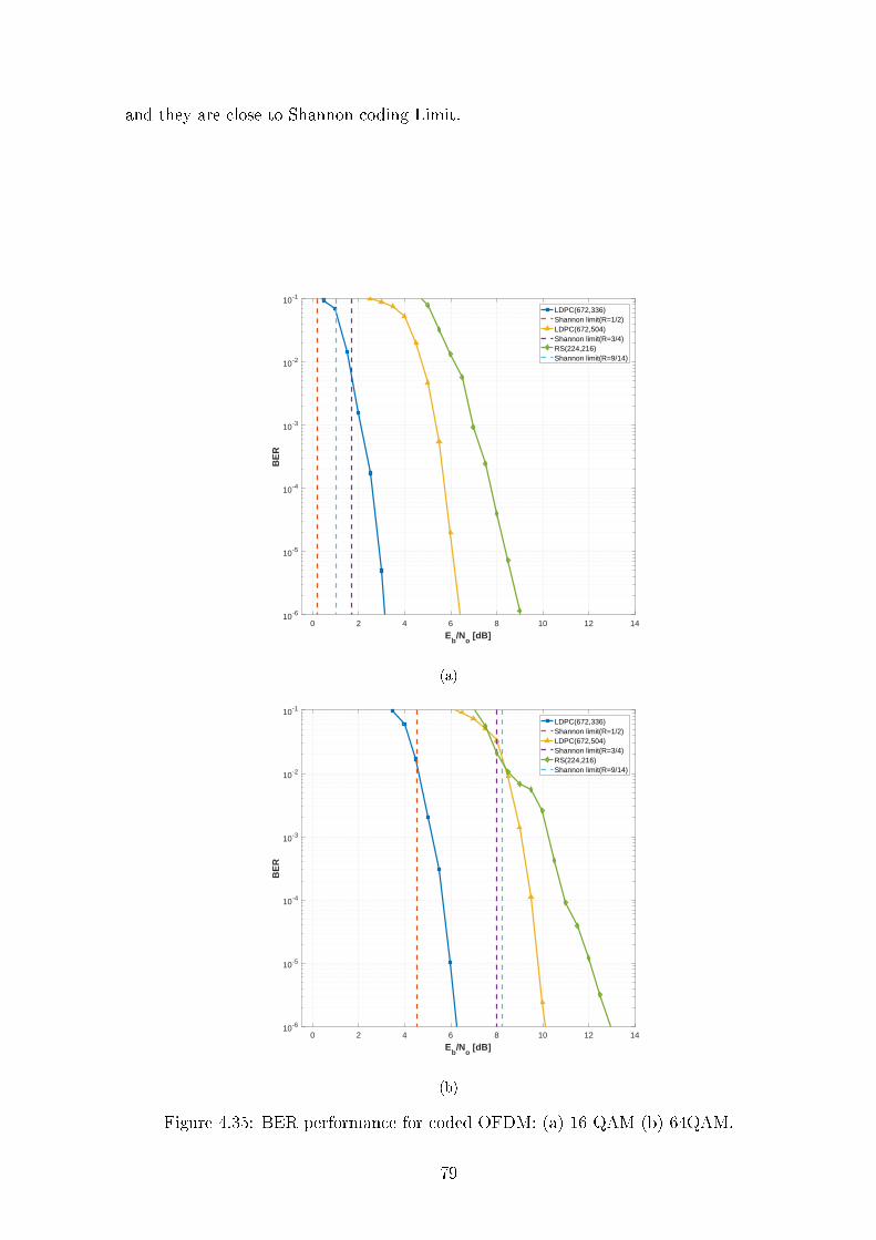
and they are close to Shannon coding Limit.
0 2 4 6 8 10 12 14
Eb/N
o [dB]
10-6
10-5
10-4
10-3
10-2
10-1
BE
R
LDPC(672,336)Shannon limit(R=1/2)LDPC(672,504)Shannon limit(R=3/4)RS(224,216)Shannon limit(R=9/14)
(a)
0 2 4 6 8 10 12 14
Eb/N
o [dB]
10-6
10-5
10-4
10-3
10-2
10-1
BE
R
LDPC(672,336)Shannon limit(R=1/2)LDPC(672,504)Shannon limit(R=3/4)RS(224,216)Shannon limit(R=9/14)
(b)
Figure 4.35: BER performance for coded OFDM: (a) 16 QAM (b) 64QAM.
79

4.12 Summary
Chapter 4 presented the implementation of the proposed simulation framework. First,
the general block diagram of the framework is shown and a quick description of the
overall operation is presented. Then, each block of general block diagram is detailed.
This Chapter also addresses the performance evaluation metric considered for the work
in order to characterize properly the framework performance. Finally, simulation re-
sults are conducted in order to validate the simulation tool.
80
Chapter 5
Performance evaluation of 60 GHz OFDM
framework over indoor multipath fad-
ing channels
5.1 Introduction
This section aims to present the results of the performance evaluation of the previously
presented multi-gigabit simulation framework at 60 GHz towards 5G communications.
The objective of this evaluation is to characterize the performance of the simulation
environment based on a realistic OFDM transmission at 60 GHz band. For that, the
key performance indicator presented in the previous Section are considered.
In order to present a more realistic performance results, the considered multipath
fading channels were extracted from real measurements for both LOS and NLOS envi-
ronments. The need of a quasi-realistic simulation led to consider a stable standard at
60 GHz band, the IEEE 802.15.3c standard which is specied for high rate wireless per-
sonal area networks (WPANs) (Section 2.3.2). Thus, in this section several simulation
parameters are obtained from the IEEE 50.15.3c standard.
Since the main goal of the proposed framework is to provide a high data rate
transmission at 60 GHz, the distance between transmitter and receiver is relatively
low. Thus, only indoor scenarios are considered for performance evaluation purposes.
Thus, in this section, rstly, the scenarios considered for the performance evaluation
are presented and the indoor environments are presented and characterized. Then,
the performance results of the uncoded and coded transmission are presented. After
81
that, a comparative analysis of both channel estimation techniques is shown. Finally,
uncompressed video is transmitted over the implemented framework and the results
are drawn.
5.2 Study scenarios
The considered indoor scenarios are based on real measurements at 60 GHz band for
both LOS and NLOS typologies. In this section the measurement results are shown,
as well as the link budget of the considered wireless transmission. It is also taken
into account the mobility eect due to the movement of persons in the interior of the
building.
5.2.1 Indoor environments
This section presents the channel modeling proposed by TG3c [22] at 60 GHz for the
indoor environments: residential, oce and kiosk. Each environment can be classied
as Line-Of-Sight (LOS) or Non-Line-Of-Sight (NLOS). For LOS, it is considered that
there are no objects that block the direct path between the transmitter (TX) and the
receiver (RX). In an LOS indoor scenario the multipath are mainly from reected or
scattered signals from furniture, the oor and the ceiling. For a NLOS scenario there
are no direct path between the transmitter and the receiver antenna.
The residential environment considers, for example, a typical home with multiple
rooms and furnished with furniture and TVs sets lounges. The size is comparable to a
small oce room and the wall is made of concrete or wood. There are also windows
and wooden door in dierent rooms.
Typical oce environment contains multiple chairs, desks, computers, and work
stations. The walls are made of metal or concrete covered by plasterboard or carpet.
This environment type is, typically linked by long corridors.
Kiosk describes a situation where a person is in front of the kiosk serve holding a
portable device. Usually, the portable device is pointed to the kiosk server.
For residential environment, both LOS and NLOS scenarios were considered, result-
82
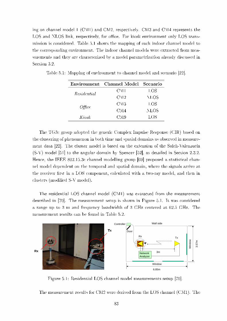
ing on channel model 1 (CM1) and CM2, respectively. CM3 and CM4 represents the
LOS and NLOS link, respectively, for oce. For kiosk environment only LOS trans-
mission is considered. Table 5.1 shows the mapping of each indoor channel model to
the corresponding environment. The indoor channel models were extracted from mea-
surements and they are characterized by a model parametrization already discussed in
Section 3.2.
Table 5.1: Mapping of environment to channel model and scenario [22].
Environment Channel Model Scenario
ResidentialCM1 LOS
CM2 NLOS
OceCM3 LOS
CM4 NLOS
Kiosk CM9 LOS
The TG3c group adopted the generic Complex Impulse Response (CIR) based on
the clustering of phenomenon in both time and spatial domains as observed in measure-
ment data [22]. The cluster model is based on the extension of the Saleh-Valenzuela
(S-V) model [51] to the angular domain by Spencer [52], as detailed in Section 2.3.2.
Hence, the IEEE 802.15.3c channel modelling group [69] proposed a statistical chan-
nel model dependent on the temporal and spatial domain, where the signals arrive at
the receiver rst in a LOS component, calculated with a two-ray model, and then in
clusters (modied S-V model).
The residential LOS channel model (CM1) was extracted from the measurement
described in [70]. The measurement setup is shown in Figure 5.1. It was considered
a range up to 3 m and frequency bandwidth of 3 GHz centered at 62.5 GHz. The
measurement results can be found in Table 5.2.
3m
Door
TxRx
Win
dow
Wall side
Window
Controller
6.85m
3.5
7m
Network
Analyzer
Tx
Rx
Figure 5.1: Residential LOS channel model measurements setup [70].
The measurement results for CM2 were derived from the LOS channel (CM1). The
83
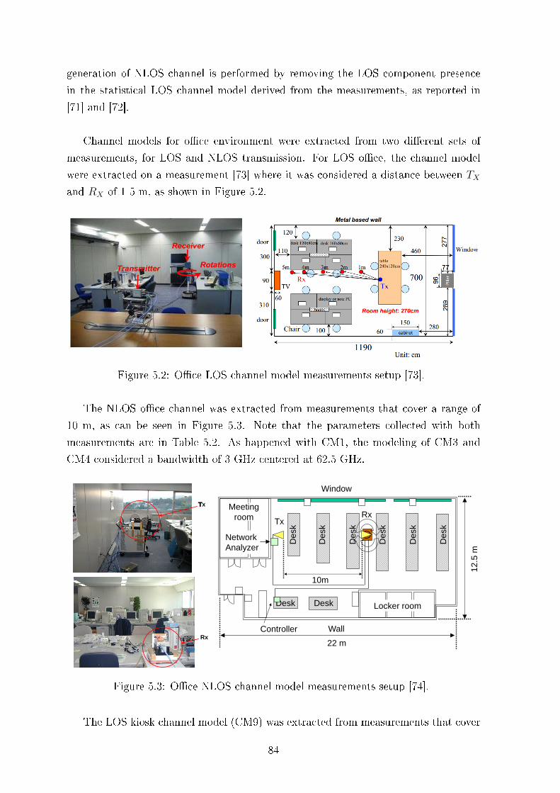
generation of NLOS channel is performed by removing the LOS component presence
in the statistical LOS channel model derived from the measurements, as reported in
[71] and [72].
Channel models for oce environment were extracted from two dierent sets of
measurements, for LOS and NLOS transmission. For LOS oce, the channel model
were extracted on a measurement [73] where it was considered a distance between TXand RX of 1-5 m, as shown in Figure 5.2.
Figure 5.2: Oce LOS channel model measurements setup [73].
The NLOS oce channel was extracted from measurements that cover a range of
10 m, as can be seen in Figure 5.3. Note that the parameters collected with both
measurements are in Table 5.2. As happened with CM1, the modeling of CM3 and
CM4 considered a bandwidth of 3 GHz centered at 62.5 GHz.
Wall
Window
De
sk
De
sk
Desk
Desk
Desk
De
sk
Desk Desk
Meeting
room
Locker room
TxRx
Controller
10m
22 m
12
.5 m
Network
Analyzer
Tx
Rx
Figure 5.3: Oce NLOS channel model measurements setup [74].
The LOS kiosk channel model (CM9) was extracted from measurements that cover
84
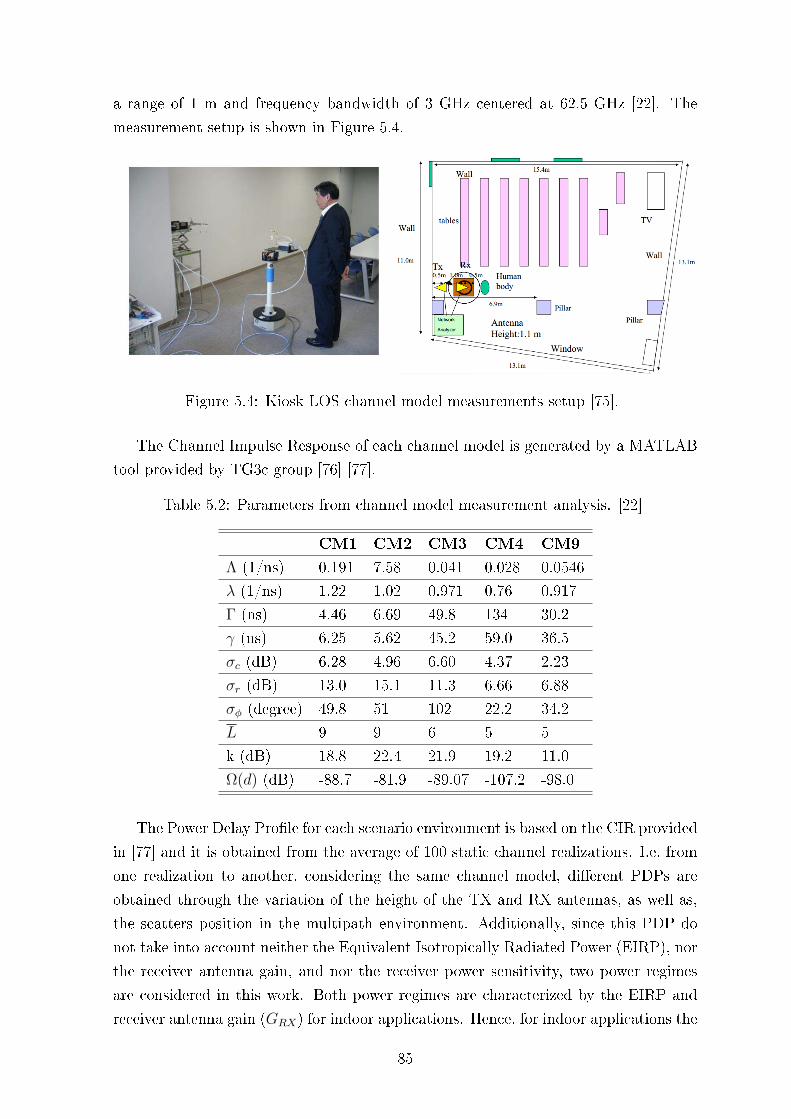
a range of 1 m and frequency bandwidth of 3 GHz centered at 62.5 GHz [22]. The
measurement setup is shown in Figure 5.4.
Figure 5.4: Kiosk LOS channel model measurements setup [75].
The Channel Impulse Response of each channel model is generated by a MATLAB
tool provided by TG3c group [76] [77].
Table 5.2: Parameters from channel model measurement analysis. [22]
CM1 CM2 CM3 CM4 CM9
Λ (1/ns) 0.191 7.58 0.041 0.028 0.0546
λ (1/ns) 1.22 1.02 0.971 0.76 0.917
Γ (ns) 4.46 6.69 49.8 134 30.2
γ (ns) 6.25 5.62 45.2 59.0 36.5
σc (dB) 6.28 4.96 6.60 4.37 2.23
σr (dB) 13.0 15.1 11.3 6.66 6.88
σφ (degree) 49.8 51 102 22.2 34.2
L 9 9 6 5 5
k (dB) 18.8 22.4 21.9 19.2 11.0
Ω(d) (dB) -88.7 -81.9 -89.07 -107.2 -98.0
The Power Delay Prole for each scenario environment is based on the CIR provided
in [77] and it is obtained from the average of 100 static channel realizations. I.e, from
one realization to another, considering the same channel model, dierent PDPs are
obtained through the variation of the height of the TX and RX antennas, as well as,
the scatters position in the multipath environment. Additionally, since this PDP do
not take into account neither the Equivalent Isotropically Radiated Power (EIRP), nor
the receiver antenna gain, and nor the receiver power sensitivity, two power regimes
are considered in this work. Both power regimes are characterized by the EIRP and
receiver antenna gain (GRX) for indoor applications. Hence, for indoor applications the
85
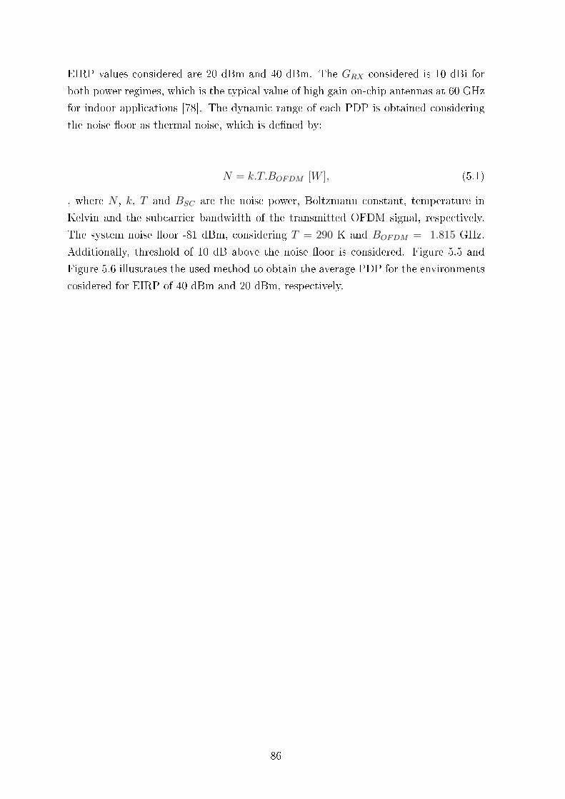
EIRP values considered are 20 dBm and 40 dBm. The GRX considered is 10 dBi for
both power regimes, which is the typical value of high gain on-chip antennas at 60 GHz
for indoor applications [78]. The dynamic range of each PDP is obtained considering
the noise oor as thermal noise, which is dened by:
N = k.T.BOFDM [W ], (5.1)
, where N , k, T and BSC are the noise power, Boltzmann constant, temperature in
Kelvin and the subcarrier bandwidth of the transmitted OFDM signal, respectively.
The system noise oor -81 dBm, considering T = 290 K and BOFDM = 1.815 GHz.
Additionally, threshold of 10 dB above the noise oor is considered. Figure 5.5 and
Figure 5.6 illustrates the used method to obtain the average PDP for the environments
cosidered for EIRP of 40 dBm and 20 dBm, respectively.
86
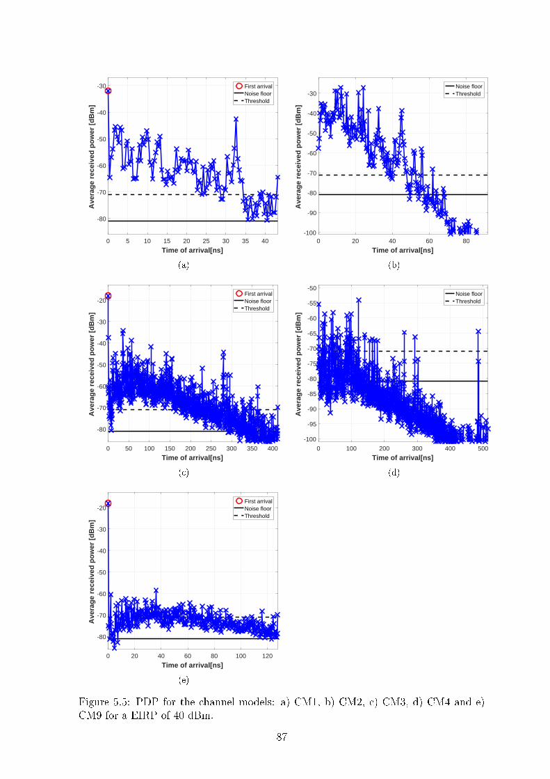
0 5 10 15 20 25 30 35 40
Time of arrival[ns]
-80
-70
-60
-50
-40
-30A
vera
ge
rece
ived
po
wer
[d
Bm
]First arrivalNoise floorThreshold
(a)
0 20 40 60 80
Time of arrival[ns]
-100
-90
-80
-70
-60
-50
-40
-30
Ave
rag
e re
ceiv
ed p
ow
er [
dB
m]
Noise floorThreshold
(b)
0 50 100 150 200 250 300 350 400
Time of arrival[ns]
-80
-70
-60
-50
-40
-30
-20
Ave
rag
e re
ceiv
ed p
ow
er [
dB
m]
First arrivalNoise floorThreshold
(c)
0 100 200 300 400 500
Time of arrival[ns]
-100
-95
-90
-85
-80
-75
-70
-65
-60
-55
-50
Ave
rag
e re
ceiv
ed p
ow
er [
dB
m]
Noise floorThreshold
(d)
0 20 40 60 80 100 120
Time of arrival[ns]
-80
-70
-60
-50
-40
-30
-20
Ave
rag
e re
ceiv
ed p
ow
er [
dB
m]
First arrivalNoise floorThreshold
(e)
Figure 5.5: PDP for the channel models: a) CM1, b) CM2, c) CM3, d) CM4 and e)CM9 for a EIRP of 40 dBm.
87
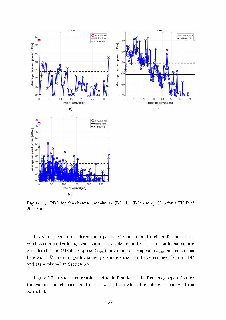
0 5 10 15 20 25 30
Time of arrival[ns]
-85
-80
-75
-70
-65
-60
-55
-50
Ave
rag
e re
ceiv
ed p
ow
er [
dB
m]
PDP
First arrivalNoise floorThreshold
(a)
0 10 20 30 40 50 60 70
Time of arrival[ns]
-100
-90
-80
-70
-60
-50
Ave
rag
e re
ceiv
ed p
ow
er [
dB
m]
PDP
Noise floorThreshold
(b)
0 50 100 150 200 250
Time of arrival[ns]
-85
-80
-75
-70
-65
-60
-55
-50
-45
-40
-35
Ave
rag
e re
ceiv
ed p
ow
er [
dB
m]
PDP
First arrivalNoise floorThreshold
(c)
Figure 5.6: PDP for the channel models: a) CM1, b) CM2 and c) CM3 for a EIRP of20 dBm.
In order to compare dierent multipath environments and their performance in a
wireless communication system, parameters which quantify the multipath channel are
considered. The RMS delay spread (τrms), maximum delay spread (τmax) and coherence
bandwidth Bc are multipath channel parameters that can be determined from a PDP
and are explained in Section 3.2.
Figure 5.7 shows the correlation factors in function of the frequency separation for
the channel models considered in this work, from which the coherence bandwidth is
extracted.
88
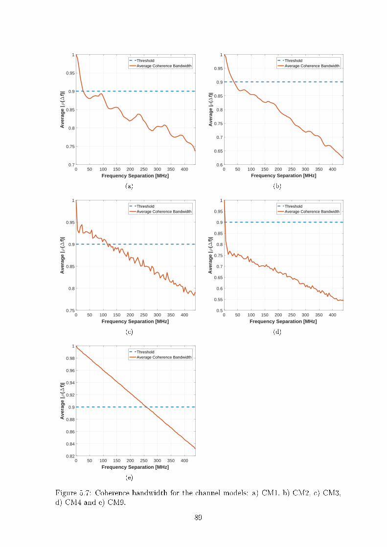
0 50 100 150 200 250 300 350 400
Frequency Separation [MHz]
0.7
0.75
0.8
0.85
0.9
0.95
1
Ave
rag
e |ρ
(∆f)
|ThresholdAverage Coherence Bandwidth
(a)
0 50 100 150 200 250 300 350 400
Frequency Separation [MHz]
0.6
0.65
0.7
0.75
0.8
0.85
0.9
0.95
1
Ave
rag
e |ρ
(∆f)
|
ThresholdAverage Coherence Bandwidth
(b)
0 50 100 150 200 250 300 350 400
Frequency Separation [MHz]
0.75
0.8
0.85
0.9
0.95
1
Ave
rag
e |ρ
(∆f)
|
ThresholdAverage Coherence Bandwidth
(c)
0 50 100 150 200 250 300 350 400
Frequency Separation [MHz]
0.5
0.55
0.6
0.65
0.7
0.75
0.8
0.85
0.9
0.95
1
Ave
rag
e |ρ
(∆f)
|ThresholdAverage Coherence Bandwidth
(d)
0 50 100 150 200 250 300 350 400
Frequency Separation [MHz]
0.82
0.84
0.86
0.88
0.9
0.92
0.94
0.96
0.98
1
Ave
rag
e |ρ
(∆f)
|
ThresholdAverage Coherence Bandwidth
(e)
Figure 5.7: Coherence bandwidth for the channel models: a) CM1, b) CM2, c) CM3,d) CM4 and e) CM9.
89
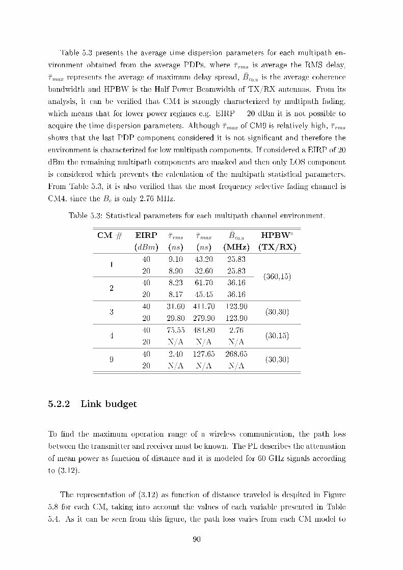
Table 5.3 presents the average time dispersion parameters for each multipath en-
vironment obtained from the average PDPs, where τ rms is average the RMS delay,
τmax represents the average of maximum delay spread, Bc0.9 is the average coherence
bandwidth and HPBW is the Half Power Beamwidth of TX/RX antennas. From its
analysis, it can be veried that CM4 is strongly characterized by multipath fading,
which means that for lower power regimes e.g. EIRP = 20 dBm it is not possible to
acquire the time dispersion parameters. Although τmax of CM9 is relatively high, τ rmsshows that the last PDP component considered it is not signicant and therefore the
environment is characterized for low multipath components. If considered a EIRP of 20
dBm the remaining multipath components are masked and then only LOS component
is considered which prevents the calculation of the multipath statistical parameters.
From Table 5.3, it is also veried that the most frequency selective fading channel is
CM4, since the Bc is only 2.76 MHz.
Table 5.3: Statistical parameters for each multipath channel environment.
CM # EIRP
(dBm)
τ rms
(ns)
τmax
(ns)
Bc0.9
(MHz)
HPBW
(TX/RX)
140 9.10 43.20 25.83
(360,15)20 8.90 32.60 25.83
240 8.23 61.70 36.16
20 8.17 45.45 36.16
340 31.60 411.70 123.90
(30,30)20 29.80 279.90 123.90
440 75.55 484.80 2.76
(30,15)20 N/A N/A N/A
940 2.40 127.65 268.65
(30,30)20 N/A N/A N/A
5.2.2 Link budget
To nd the maximum operation range of a wireless communication, the path loss
between the transmitter and receiver must be known. The PL describes the attenuation
of mean power as function of distance and it is modeled for 60 GHz signals according
to (3.12).
The representation of (3.12) as function of distance traveled is despited in Figure
5.8 for each CM, taking into account the values of each variable presented in Table
5.4. As it can be seen from this gure, the path loss varies from each CM model to
90
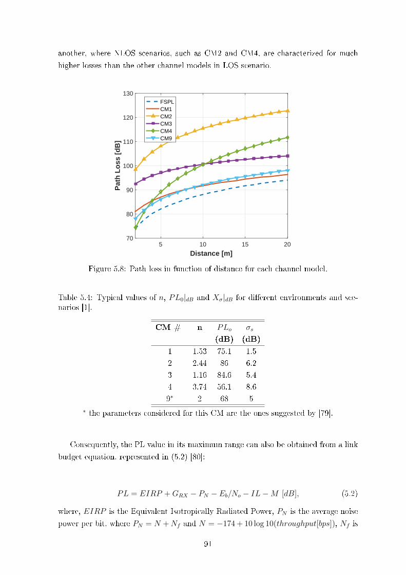
another, where NLOS scenarios, such as CM2 and CM4, are characterized for much
higher losses than the other channel models in LOS scenario.
Distance [m]5 10 15 20
Pat
h L
oss
[d
B]
70
80
90
100
110
120
130FSPLCM1CM2CM3CM4CM9
Figure 5.8: Path loss in function of distance for each channel model.
Table 5.4: Typical values of n, PL0|dB and Xσ|dB for dierent environments and sce-narios [1].
CM # n PLo
(dB)
σs
(dB)
1 1.53 75.1 1.5
2 2.44 86 6.2
3 1.16 84.6 5.4
4 3.74 56.1 8.6
9∗ 2 68 5∗ the parameters considered for this CM are the ones suggested by [79].
Consequently, the PL value in its maximum range can also be obtained from a link
budget equation, represented in (5.2) [80]:
PL = EIRP +GRX − PN − Eb/No − IL−M [dB], (5.2)
where, EIRP is the Equivalent Isotropically Radiated Power, PN is the average noise
power per bit, where PN = N +Nf and N = −174 + 10 log 10(throughput[bps]), Nf is
91
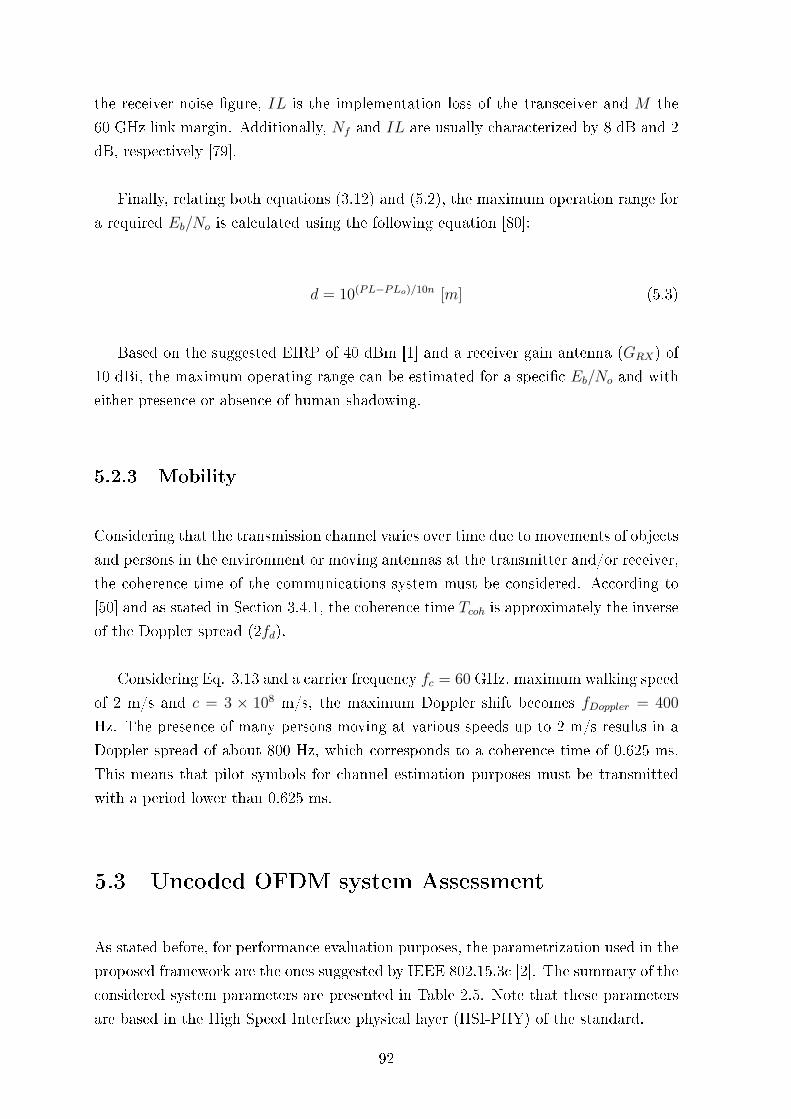
the receiver noise gure, IL is the implementation loss of the transceiver and M the
60 GHz link margin. Additionally, Nf and IL are usually characterized by 8 dB and 2
dB, respectively [79].
Finally, relating both equations (3.12) and (5.2), the maximum operation range for
a required Eb/No is calculated using the following equation [80]:
d = 10(PL−PLo)/10n [m] (5.3)
Based on the suggested EIRP of 40 dBm [1] and a receiver gain antenna (GRX) of
10 dBi, the maximum operating range can be estimated for a specic Eb/No and with
either presence or absence of human shadowing.
5.2.3 Mobility
Considering that the transmission channel varies over time due to movements of objects
and persons in the environment or moving antennas at the transmitter and/or receiver,
the coherence time of the communications system must be considered. According to
[50] and as stated in Section 3.4.1, the coherence time Tcoh is approximately the inverse
of the Doppler spread (2fd).
Considering Eq. 3.13 and a carrier frequency fc = 60 GHz, maximum walking speed
of 2 m/s and c = 3 × 10⁸ m/s, the maximum Doppler shift becomes fDoppler = 400
Hz. The presence of many persons moving at various speeds up to 2 m/s results in a
Doppler spread of about 800 Hz, which corresponds to a coherence time of 0.625 ms.
This means that pilot symbols for channel estimation purposes must be transmitted
with a period lower than 0.625 ms.
5.3 Uncoded OFDM system Assessment
As stated before, for performance evaluation purposes, the parametrization used in the
proposed framework are the ones suggested by IEEE 802.15.3c [2]. The summary of the
considered system parameters are presented in Table 2.5. Note that these parameters
are based in the High Speed Interface physical layer (HSI-PHY) of the standard.
92
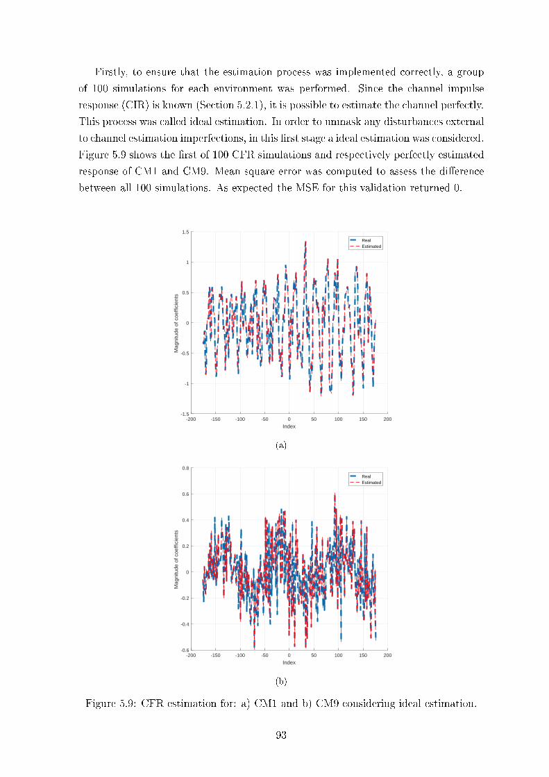
Firstly, to ensure that the estimation process was implemented correctly, a group
of 100 simulations for each environment was performed. Since the channel impulse
response (CIR) is known (Section 5.2.1), it is possible to estimate the channel perfectly.
This process was called ideal estimation. In order to unmask any disturbances external
to channel estimation imperfections, in this rst stage a ideal estimation was considered.
Figure 5.9 shows the rst of 100 CFR simulations and respectively perfectly estimated
response of CM1 and CM9. Mean square error was computed to assess the dierence
between all 100 simulations. As expected the MSE for this validation returned 0.
-200 -150 -100 -50 0 50 100 150 200
Index
-1.5
-1
-0.5
0
0.5
1
1.5
Mag
nitu
de o
f coe
ffici
ents
RealEstimated
(a)
-200 -150 -100 -50 0 50 100 150 200
Index
-0.6
-0.4
-0.2
0
0.2
0.4
0.6
0.8
Mag
nitu
de o
f coe
ffici
ents
RealEstimated
(b)
Figure 5.9: CFR estimation for: a) CM1 and b) CM9 considering ideal estimation.
93
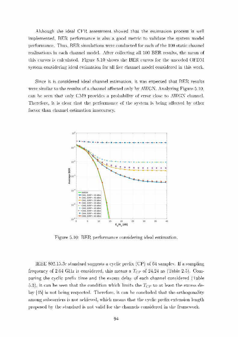
Although the ideal CFR assessment showed that the estimation process is well
implemented, BER performance is also a good metric to validate the system model
performance. Thus, BER simulations were conducted for each of the 100 static channel
realizations in each channel model. After collecting all 100 BER results, the mean of
this curves is calculated. Figure 5.10 shows the BER curves for the uncoded OFDM
system considering ideal estimation for all ve channel model considered in this work.
Since it is considered ideal channel estimation, it was expected that BER results
were similar to the results of a channel aected only by AWGN. Analyzing Figure 5.10,
can be seen that only CM9 provides a probability of error close to AWGN channel.
Therefore, it is clear that the performance of the system is being aected by other
factor than channel estimation inaccuracy.
0 5 10 15 20 25 30 35 40
Eb/N
o [dB]
10-6
10-5
10-4
10-3
10-2
10-1
100
Ave
rag
e B
ER
AWGNCM1, EIRP = 20 dBmCM1, EIRP = 40 dBmCM2, EIRP = 20 dBmCM2, EIRP = 40 dBmCM3, EIRP = 20 dBmCM3, EIRP = 40 dBmCM4, EIRP = 20 dBmCM4, EIRP = 40 dBmCM9, EIRP = 40 dBm
Figure 5.10: BER performance considering ideal estimation.
IEEE 802.15.3c standard suggests a cyclic prex (CP) of 64 samples. If a sampling
frequency of 2.64 GHz is considered, this means a TCP of 24.24 ns (Table 2.5). Com-
paring the cyclic prex time and the excess delay of each channel considered (Table
5.3), it can be seen that the condition which limits the TCP to at least the excess de-
lay [45] is not being respected. Therefore, it can be concluded that the orthogonality
among subcarriers is not achieved, which means that the cyclic prex extension length
proposed by the standard is not valid for the channels considered in the framework.
94
5.3.1 Cyclic prex length: parametric study
In order to improve the performance of the system, larger cyclic prexes must be
considered. Extending the CP leads to an increment of the system's overhead because
more redundant information is transmitted, which leads also to a decrement of spectral
eciency. Therefore is mandatory to nd a trade-o that ensures good performance
with the minimum introduced overhead.
First, is important to assess the impact of the TCP in the BER results for the channel
models considered. For that, several simulations varying the TCP were conducted and
the result of such simulations are drawn in Figure 5.11. Note that is considered uncoded
transmission, 16 QAM modulation, ZF equalization, ideal estimation and a EIRP of
40 dBm. Figure 5.11 shows the dierent BER results when changing only the CP
length. It can be seen that CP strongly aects the overall system performance and
needs to be dened based on the environment considered. From Figure 5.11 it is
also possible to conclude that, for CM3 and CM4, a CP with the same length as the
OFDM symbol is not enough to ensure good results. It means that only CP multiple
of the OFDM symbol length could, eventually improve the BER performance og these
channel models. Therefore, it would deteriorate signicantly the spectral eciency.
For that reason, simulation results referring CM3 and CM4 will not be analyzed in
this document. Note that, as expected, the uncoded performance for CM9 is not
signicantly aected by the length of CP, since for a TCP=24.24 ns (Figure 5.10) it
was already obtained good results.
Consider a TCP signicantly large comparing to the excess delay (τmax) of the chan-
nel may lead to a unnecessary overhead, which compromises the system's throughput.
Thus, a parametric study were conducted to nd the most suitable length of CP for
each environment. From this study it was concluded that consider TCP ' τmax is an
appropriate metric since it ensures good BER performance and does not reduce sig-
nicantly the throughput. The results of the TCP study are drawn in Table 5.5 where
can be seen the required EbN0 to ensure a BER of 10−6 for both 16 and 64 QAM
modulation.
95
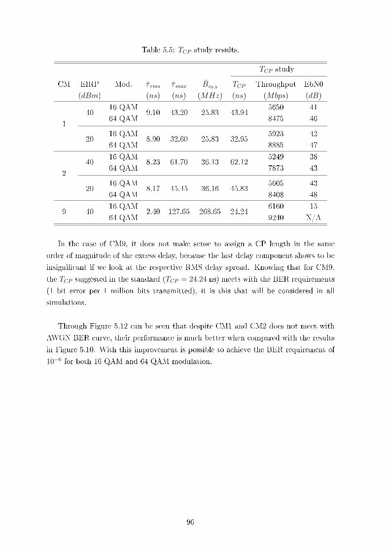
Table 5.5: TCP study results.
TCP study
CM EIRP Mod. τ rms τmax Bc0.9 TCP Throughput EbN0
(dBm) (ns) (ns) (MHz) (ns) (Mbps) (dB)
1
4016 QAM
9.10 43.20 25.83 43.945650 41
64 QAM 8475 46
2016 QAM
8.90 32.60 25.83 32.955923 42
64 QAM 8885 47
2
4016 QAM
8.23 61.70 36.13 62.125249 38
64 QAM 7873 43
2016 QAM
8.17 45.45 36.16 45.835605 43
64 QAM 8408 48
9 4016 QAM
2.40 127.65 268.65 24.246160 15
64 QAM 9240 N/A
In the case of CM9, it does not make sense to assign a CP length in the same
order of magnitude of the excess delay, because the last delay component shows to be
insignicant if we look at the respective RMS delay spread. Knowing that for CM9,
the TCP suggested in the standard (TCP = 24.24 ns) meets with the BER requirements
(1 bit error per 1 million bits transmitted), it is this that will be considered in all
simulations.
Through Figure 5.12 can be seen that despite CM1 and CM2 does not meet with
AWGN BER curve, their performance is much better when compared with the results
in Figure 5.10. With this improvement is possible to achieve the BER requirement of
10−6 for both 16 QAM and 64 QAM modulation.
96
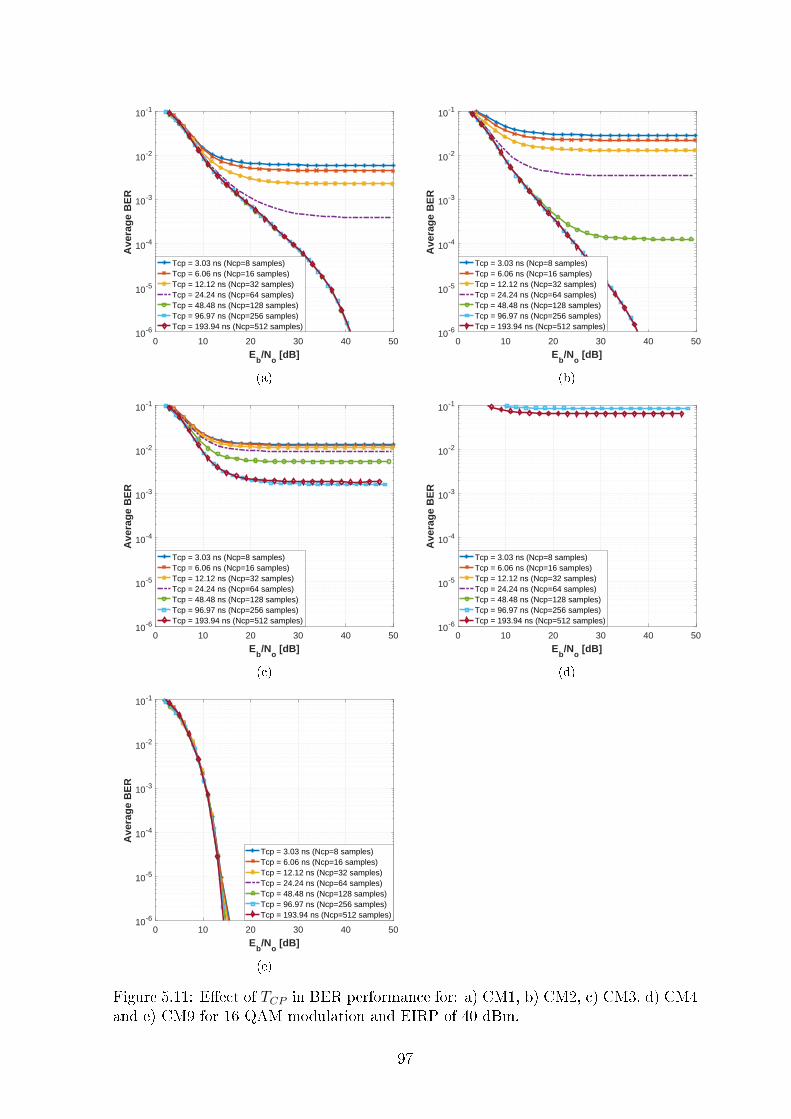
0 10 20 30 40 50
Eb/N
o [dB]
10-6
10-5
10-4
10-3
10-2
10-1
Ave
rag
e B
ER
Tcp = 3.03 ns (Ncp=8 samples)Tcp = 6.06 ns (Ncp=16 samples)Tcp = 12.12 ns (Ncp=32 samples)Tcp = 24.24 ns (Ncp=64 samples)Tcp = 48.48 ns (Ncp=128 samples)Tcp = 96.97 ns (Ncp=256 samples)Tcp = 193.94 ns (Ncp=512 samples)
(a)
0 10 20 30 40 50
Eb/N
o [dB]
10-6
10-5
10-4
10-3
10-2
10-1
Ave
rag
e B
ER
Tcp = 3.03 ns (Ncp=8 samples)Tcp = 6.06 ns (Ncp=16 samples)Tcp = 12.12 ns (Ncp=32 samples)Tcp = 24.24 ns (Ncp=64 samples)Tcp = 48.48 ns (Ncp=128 samples)Tcp = 96.97 ns (Ncp=256 samples)Tcp = 193.94 ns (Ncp=512 samples)
(b)
0 10 20 30 40 50
Eb/N
o [dB]
10-6
10-5
10-4
10-3
10-2
10-1
Ave
rag
e B
ER
Tcp = 3.03 ns (Ncp=8 samples)Tcp = 6.06 ns (Ncp=16 samples)Tcp = 12.12 ns (Ncp=32 samples)Tcp = 24.24 ns (Ncp=64 samples)Tcp = 48.48 ns (Ncp=128 samples)Tcp = 96.97 ns (Ncp=256 samples)Tcp = 193.94 ns (Ncp=512 samples)
(c)
0 10 20 30 40 50
Eb/N
o [dB]
10-6
10-5
10-4
10-3
10-2
10-1
Ave
rag
e B
ER
Tcp = 3.03 ns (Ncp=8 samples)Tcp = 6.06 ns (Ncp=16 samples)Tcp = 12.12 ns (Ncp=32 samples)Tcp = 24.24 ns (Ncp=64 samples)Tcp = 48.48 ns (Ncp=128 samples)Tcp = 96.97 ns (Ncp=256 samples)Tcp = 193.94 ns (Ncp=512 samples)
(d)
0 10 20 30 40 50
Eb/N
o [dB]
10-6
10-5
10-4
10-3
10-2
10-1
Ave
rag
e B
ER
Tcp = 3.03 ns (Ncp=8 samples)Tcp = 6.06 ns (Ncp=16 samples)Tcp = 12.12 ns (Ncp=32 samples)Tcp = 24.24 ns (Ncp=64 samples)Tcp = 48.48 ns (Ncp=128 samples)Tcp = 96.97 ns (Ncp=256 samples)Tcp = 193.94 ns (Ncp=512 samples)
(e)
Figure 5.11: Eect of TCP in BER performance for: a) CM1, b) CM2, c) CM3, d) CM4and e) CM9 for 16 QAM modulation and EIRP of 40 dBm.
97
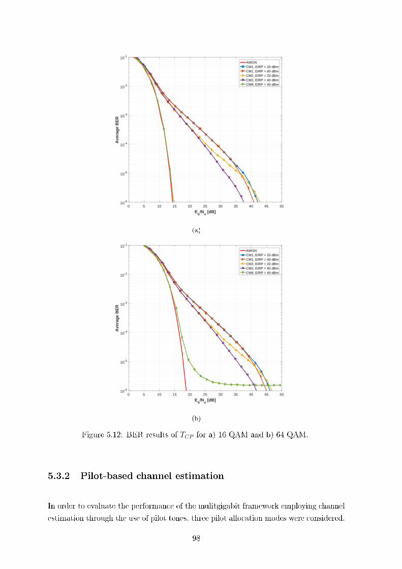
0 5 10 15 20 25 30 35 40 45 50
Eb/N
o [dB]
10-6
10-5
10-4
10-3
10-2
10-1
Ave
rag
e B
ER
AWGNCM1, EIRP = 20 dBmCM1, EIRP = 40 dBmCM2, EIRP = 20 dBmCM2, EIRP = 40 dBmCM9, EIRP = 40 dBm
(a)
0 5 10 15 20 25 30 35 40 45 50
Eb/N
o [dB]
10-6
10-5
10-4
10-3
10-2
10-1
Ave
rag
e B
ER
AWGNCM1, EIRP = 20 dBmCM1, EIRP = 40 dBmCM2, EIRP = 20 dBmCM2, EIRP = 40 dBmCM9, EIRP = 40 dBm
(b)
Figure 5.12: BER results of TCP for a) 16 QAM and b) 64 QAM.
5.3.2 Pilot-based channel estimation
In order to evaluate the performance of the mulitgigabit framework employing channel
estimation through the use of pilot tones, three pilot allocation modes were considered.
98
One of the pilot allocation modes is based on the IEEE 802.15.3c standard [2] suggestion
that implements a comb type pilot arrangement, as detailed in Section 2.3.2. The other
mode consists also in a comb type allocation, but considering pilot tones equally spaced
along with the OFDM symbol. Finally the performance of channel estimation block is
assessed applying a block type allocation method.
If pilot tones are inserted into the OFDM symbol according to an uniform distri-
bution, Xl(k) can be expressed by Eq. 5.4 [57].
Xl(k) = Xl(mL+ n) =
xp(m), n = 0
Data, n = 1, ...L− 1(5.4)
where L represents the number of subcarriers between pilots and xp(m) the value of
the mth pilot subcarrier.
Note that the number of subcarriers between pilots should be limited by the coher-
ence bandwidth of each fading channel model (Bc0.9) in order to avoid amplitude and
phase distortion [45].
If the third pilot estimation method is considered, all the subcarriers available for
data and pilots in the OFDM symbol are assigned with pilot signals, constituting a
pilot symbol. As dened in section 3.4.1, the pilot symbol must be transmitted with a
periodicity lower than the coherence time of the fading channel model (Tcoh).
Figure 5.13 and Figure 5.14 shows the multigigabit framework performance using
channel estimation based on the pilot allocation suggested in IEEE 802.15.3c standard.
In Figure 5.13 BER curves are drawn for both power regimes employing 16 QAM
modulation scheme for CM1, CM2, CM3, CM4 and CM9. It can be seen that none
of the channel models reaches de BER performance goal of 10−6, only CM9 presents
a reasonable performance. This poor results shows that the implemented channel
estimation block is not suitable for the environments considered, since the number of
pilot subcarriers proposed by IEEE 802.15.3c standard for channel estimation is not
enough to characterize the multipath channel model.
The other way to asses the poor channel estimation performance for the channel
models in this study, is to compare the estimated channel frequency response wit the
CFR known. Thus, Figure 5.14 presents the estimated CFR based on the 16 pilot
subcarriers inserted according to the standard. It is clear that the estimated CFR is
99
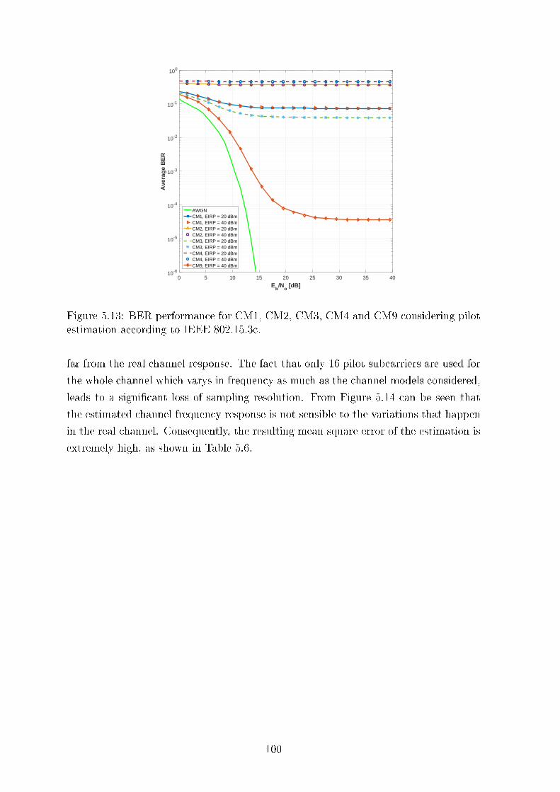
0 5 10 15 20 25 30 35 40
Eb/N
o [dB]
10-6
10-5
10-4
10-3
10-2
10-1
100
Ave
rag
e B
ER
AWGNCM1, EIRP = 20 dBmCM1, EIRP = 40 dBmCM2, EIRP = 20 dBmCM2, EIRP = 40 dBmCM3, EIRP = 20 dBmCM3, EIRP = 40 dBmCM4, EIRP = 20 dBmCM4, EIRP = 40 dBmCM9, EIRP = 40 dBm
Figure 5.13: BER performance for CM1, CM2, CM3, CM4 and CM9 considering pilotestimation according to IEEE 802.15.3c.
far from the real channel response. The fact that only 16 pilot subcarriers are used for
the whole channel which varys in frequency as much as the channel models considered,
leads to a signicant loss of sampling resolution. From Figure 5.14 can be seen that
the estimated channel frequency response is not sensible to the variations that happen
in the real channel. Consequently, the resulting mean square error of the estimation is
extremely high, as shown in Table 5.6.
100
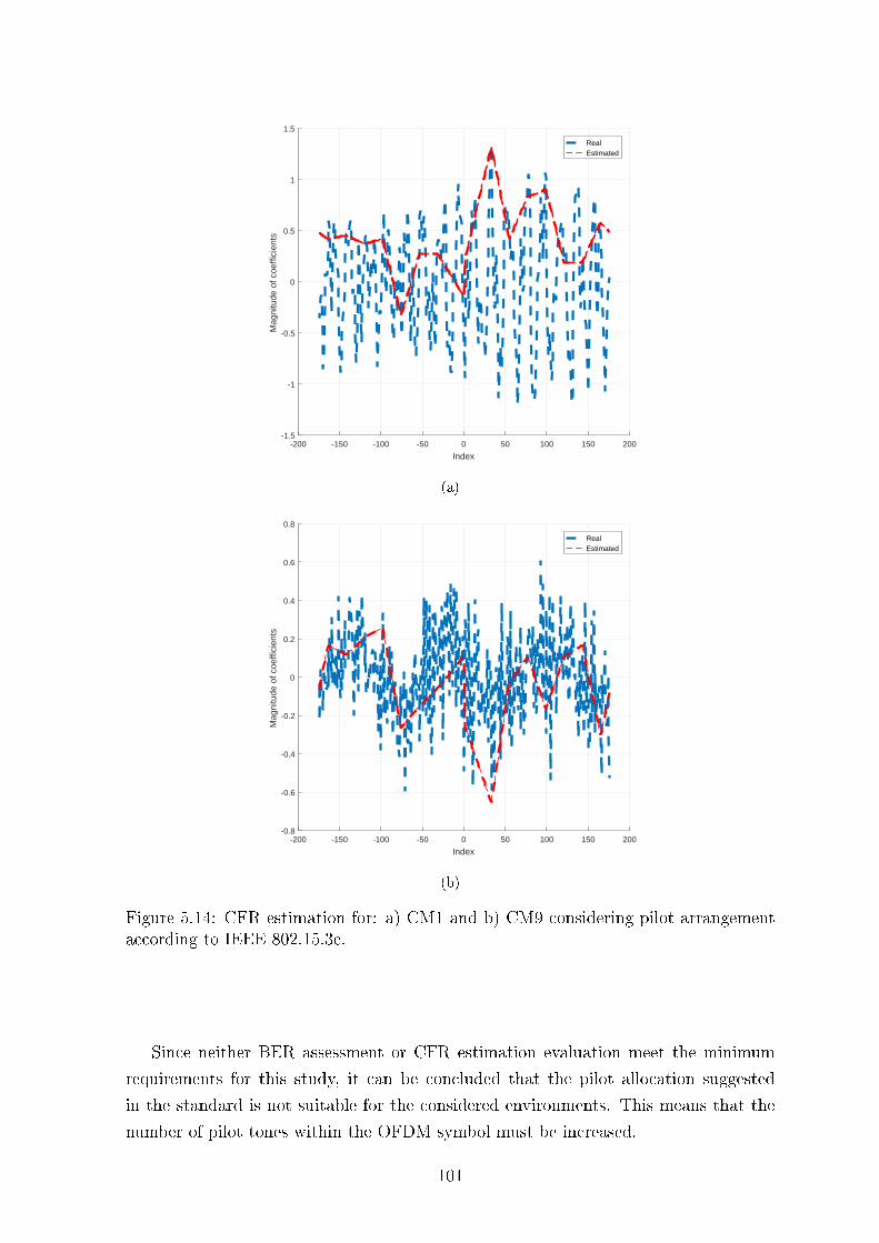
-200 -150 -100 -50 0 50 100 150 200
Index
-1.5
-1
-0.5
0
0.5
1
1.5
Mag
nitu
de o
f coe
ffici
ents
RealEstimated
(a)
-200 -150 -100 -50 0 50 100 150 200
Index
-0.8
-0.6
-0.4
-0.2
0
0.2
0.4
0.6
0.8
Mag
nitu
de o
f coe
ffici
ents
RealEstimated
(b)
Figure 5.14: CFR estimation for: a) CM1 and b) CM9 considering pilot arrangementaccording to IEEE 802.15.3c.
Since neither BER assessment or CFR estimation evaluation meet the minimum
requirements for this study, it can be concluded that the pilot allocation suggested
in the standard is not suitable for the considered environments. This means that the
number of pilot tones within the OFDM symbol must be increased.
101
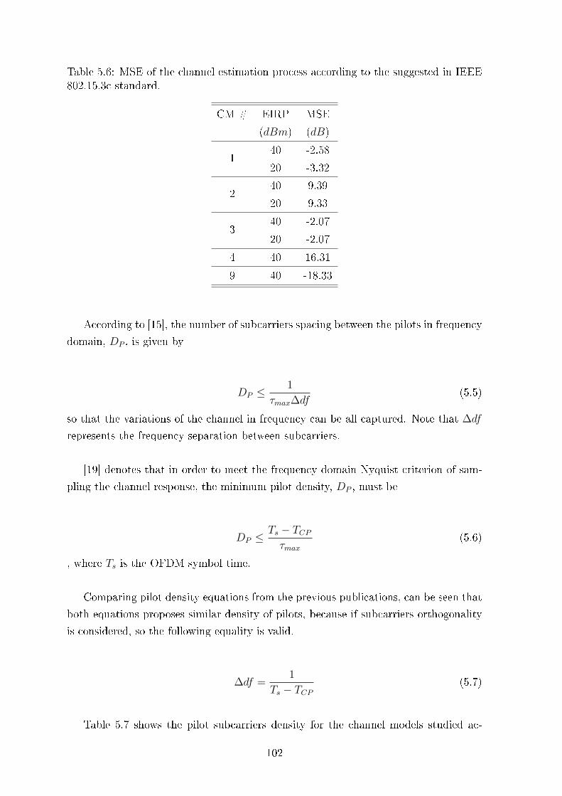
Table 5.6: MSE of the channel estimation process according to the suggested in IEEE802.15.3c standard.
CM # EIRP MSE
(dBm) (dB)
140 -2.58
20 -3.32
240 9.39
20 9.33
340 -2.07
20 -2.07
4 40 16.31
9 40 -18.33
According to [15], the number of subcarriers spacing between the pilots in frequency
domain, DP , is given by
DP ≤1
τmax∆df(5.5)
so that the variations of the channel in frequency can be all captured. Note that ∆df
represents the frequency separation between subcarriers.
[19] denotes that in order to meet the frequency domain Nyquist criterion of sam-
pling the channel response, the minimum pilot density, DP , must be
DP ≤Ts − TCPτmax
(5.6)
, where Ts is the OFDM symbol time.
Comparing pilot density equations from the previous publications, can be seen that
both equations proposes similar density of pilots, because if subcarriers orthogonality
is considered, so the following equality is valid.
∆df =1
Ts − TCP(5.7)
Table 5.7 shows the pilot subcarriers density for the channel models studied ac-
102
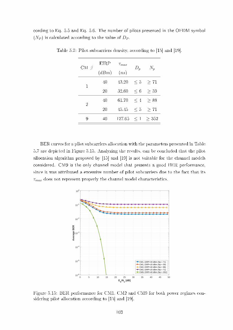
cording to Eq. 5.5 and Eq. 5.6. The number of pilots presented in the OFDM symbol
(NP ) is calculated according to the value of DP .
Table 5.7: Pilot subcarriers density, according to [15] and [19].
CM #EIRP τmax
Dp Np
(dBm) (ns)
140 43.20 ≤ 5 ≥ 71
20 32.60 ≤ 6 ≥ 59
240 61.70 ≤ 4 ≥ 88
20 45.45 ≤ 5 ≥ 71
9 40 127.65 ≤ 1 ≥ 352
BER curves for a pilot subcarriers allocation with the parameters presented in Table
5.7 are depicted in Figure 5.15. Analyzing the results, can be concluded that the pilot
allocation algorithm proposed by [15] and [19] is not suitable for the channel models
considered. CM9 is the only channel model that presents a good BER performance,
since it was attributed a excessive number of pilot subcarriers due to the fact that its
τmax does not represent properly the channel model characteristics.
0 5 10 15 20 25 30 35 40 45 50
Eb/N
o [dB]
10-6
10-5
10-4
10-3
10-2
10-1
100
Ave
rag
e B
ER
CM1, EIRP=40 dBm (Np = 71)CM1, EIRP=20 dBm (Np = 59)CM2, EIRP=40 dBm (Np = 88)CM2, EIRP=20 dBm (Np = 71)CM9, EIRP=40 dBm (Np = 352)
Figure 5.15: BER performance for CM1, CM2 and CM9 for both power regimes con-sidering pilot allocation according to [15] and [19].
103
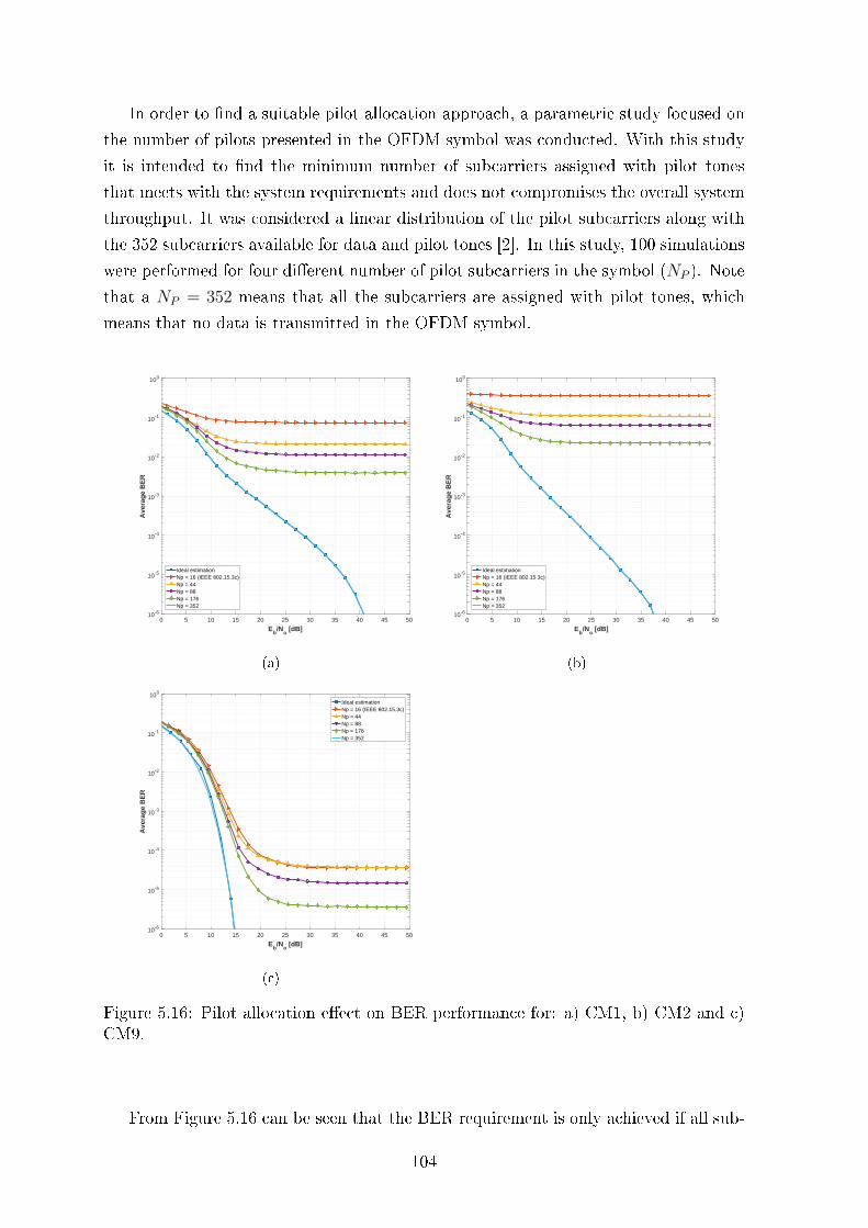
In order to nd a suitable pilot allocation approach, a parametric study focused on
the number of pilots presented in the OFDM symbol was conducted. With this study
it is intended to nd the minimum number of subcarriers assigned with pilot tones
that meets with the system requirements and does not compromises the overall system
throughput. It was considered a linear distribution of the pilot subcarriers along with
the 352 subcarriers available for data and pilot tones [2]. In this study, 100 simulations
were performed for four dierent number of pilot subcarriers in the symbol (NP ). Note
that a NP = 352 means that all the subcarriers are assigned with pilot tones, which
means that no data is transmitted in the OFDM symbol.
0 5 10 15 20 25 30 35 40 45 50
Eb/N
o [dB]
10-6
10-5
10-4
10-3
10-2
10-1
100
Ave
rag
e B
ER
Ideal estimationNp = 16 (IEEE 802.15.3c)Np = 44Np = 88Np = 176Np = 352
(a)
0 5 10 15 20 25 30 35 40 45 50
Eb/N
o [dB]
10-6
10-5
10-4
10-3
10-2
10-1
100
Ave
rag
e B
ER
Ideal estimationNp = 16 (IEEE 802.15.3c)Np = 44Np = 88Np = 176Np = 352
(b)
0 5 10 15 20 25 30 35 40 45 50
Eb/N
o [dB]
10-6
10-5
10-4
10-3
10-2
10-1
100
Ave
rag
e B
ER
Ideal estimationNp = 16 (IEEE 802.15.3c)Np = 44Np = 88Np = 176Np = 352
(c)
Figure 5.16: Pilot allocation eect on BER performance for: a) CM1, b) CM2 and c)CM9.
From Figure 5.16 can be seen that the BER requirement is only achieved if all sub-
104
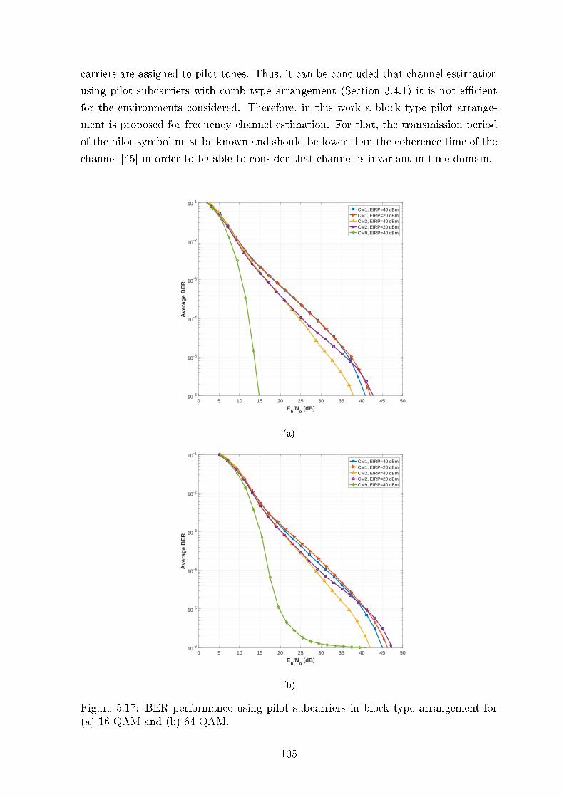
carriers are assigned to pilot tones. Thus, it can be concluded that channel estimation
using pilot subcarriers with comb type arrangement (Section 3.4.1) it is not ecient
for the environments considered. Therefore, in this work a block type pilot arrange-
ment is proposed for frequency channel estimation. For that, the transmission period
of the pilot symbol must be known and should be lower than the coherence time of the
channel [45] in order to be able to consider that channel is invariant in time-domain.
0 5 10 15 20 25 30 35 40 45 50
Eb/N
o [dB]
10-6
10-5
10-4
10-3
10-2
10-1
Ave
rag
e B
ER
CM1, EIRP=40 dBmCM1, EIRP=20 dBmCM2, EIRP=40 dBmCM2, EIRP=20 dBmCM9, EIRP=40 dBm
(a)
0 5 10 15 20 25 30 35 40 45 50
Eb/N
o [dB]
10-6
10-5
10-4
10-3
10-2
10-1
Ave
rag
e B
ER
CM1, EIRP=40 dBmCM1, EIRP=20 dBmCM2, EIRP=40 dBmCM2, EIRP=20 dBmCM9, EIRP=40 dBm
(b)
Figure 5.17: BER performance using pilot subcarriers in block type arrangement for(a) 16 QAM and (b) 64 QAM.
105
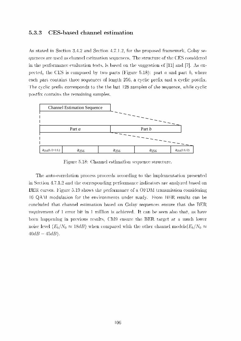
5.3.3 CES-based channel estimation
As stated in Section 3.4.2 and Section 4.7.1.2, for the proposed framework, Golay se-
quences are used as channel estimation sequences. The structure of the CES considered
in the performance evaluation tests, is based on the suggestion of [11] and [7]. As ex-
pected, the CES is composed by two parts (Figure 5.18): part a and part b, where
each part contains three sequences of length 256, a cyclic prex and a cyclic postx.
The cyclic prex corresponds to the the last 128 samples of the sequence, while cyclic
postx contains the remaining samples.
Channel Estimation Sequence
Part a Part b
a256(L/2+1:L) a256 a256 a256 a256(1:L/2)
Figure 5.18: Channel estimation sequence structure.
The auto-correlation process proceeds according to the implementation presented
in Section 4.7.1.2 and the corresponding performance indicators are analyzed based on
BER curves. Figure 5.19 shows the performance of a OFDM transmission considering
16 QAM modulation for the environments under study. From BER results can be
concluded that channel estimation based on Golay sequences ensure that the BER
requirement of 1 error bit in 1 million is achieved. It can be seen also that, as have
been happening in previous results, CM9 ensure the BER target at a much lower
noise level (Eb/N0 ≈ 18dB) when compared with the other channel models(Eb/N0 ≈40dB − 45dB).
106
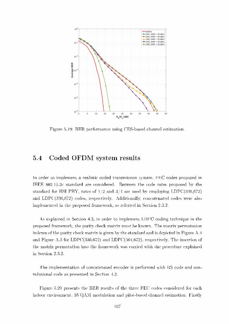
0 5 10 15 20 25 30 35 40 45 50
Eb/N
o [dB]
10-6
10-5
10-4
10-3
10-2
10-1
100
Ave
rag
e B
ER
AWGNCM1, EIRP = 20 dBmCM1, EIRP = 40 dBmCM2, EIRP = 20 dBmCM2, EIRP = 40 dBmCM9, EIRP = 40 dBm
Figure 5.19: BER performance using CES-based channel estimation.
5.4 Coded OFDM system results
In order to implement a realistic coded transmission system, FEC codes proposed in
IEEE 802.15.3c standard are considered. Between the code rates proposed by the
standard for HSI PHY, rates of 1/2 and 3/4 are used by employing LDPC(336,672)
and LDPC(336,672) codes, respectively. Additionally, concatenated codes were also
implemented in the proposed framework, as referred in Section 2.3.2.
As explained in Section 4.3, in order to implement LDPC coding technique in the
proposed framework, the parity check matrix must be known. The matrix permutation
indexes of the parity check matrix is given by the standard and is depicted in Figure A.4
and Figure A.5 for LDPC(336,672) and LDPC(504,672), respectively. The insertion of
the matrix permutation into the framework was carried with the procedure explained
in Section 2.3.2.
The implementation of concatenated encoder is performed with RS code and con-
volutional code as presented in Section 4.3.
Figure 5.20 presents the BER results of the three FEC codes considered for each
indoor environment, 16 QAM modulation and pilot-based channel estimation. Firstly
107
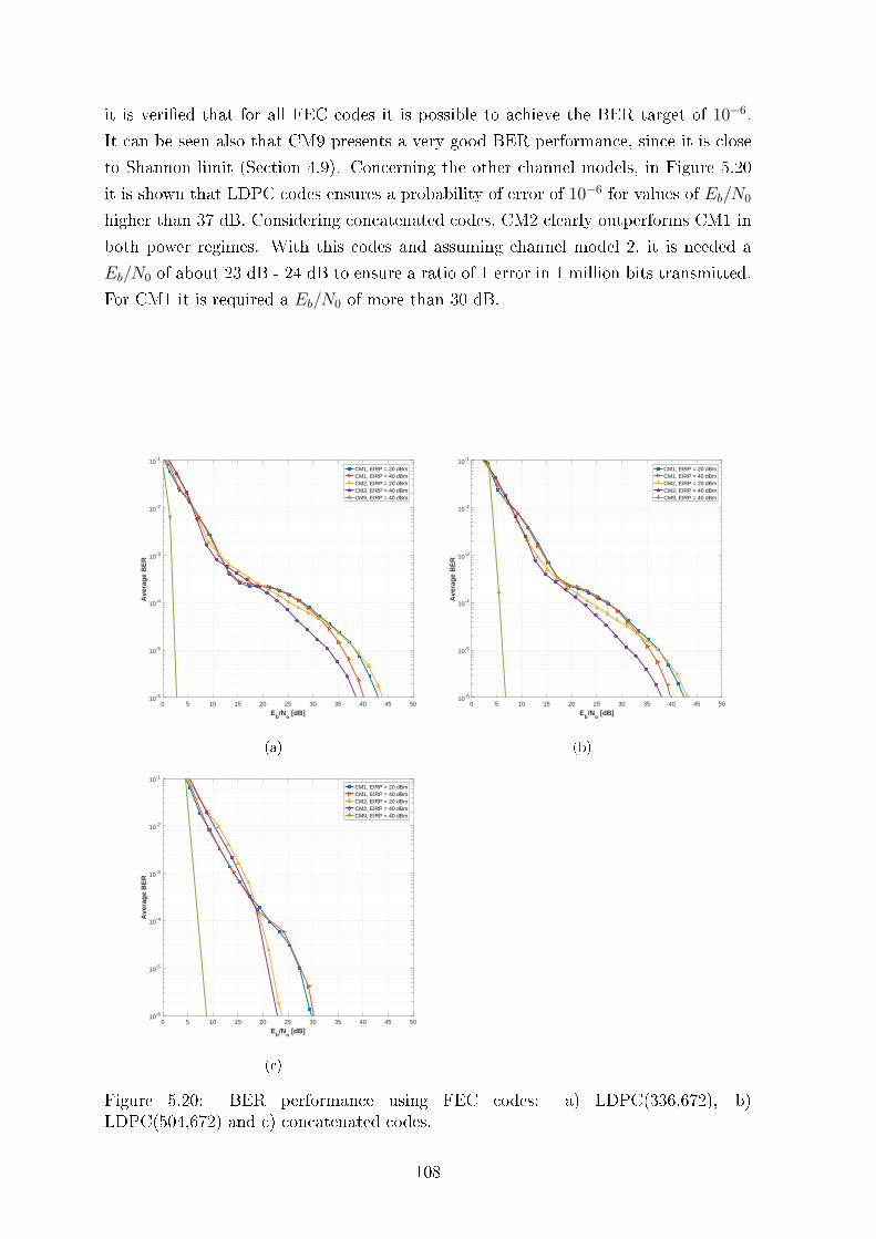
it is veried that for all FEC codes it is possible to achieve the BER target of 10−6.
It can be seen also that CM9 presents a very good BER performance, since it is close
to Shannon limit (Section 4.9). Concerning the other channel models, in Figure 5.20
it is shown that LDPC codes ensures a probability of error of 10−6 for values of Eb/N0
higher than 37 dB. Considering concatenated codes, CM2 clearly outperforms CM1 in
both power regimes. With this codes and assuming channel model 2, it is needed a
Eb/N0 of about 23 dB - 24 dB to ensure a ratio of 1 error in 1 million bits transmitted.
For CM1 it is required a Eb/N0 of more than 30 dB.
0 5 10 15 20 25 30 35 40 45 50
Eb/N
o [dB]
10-6
10-5
10-4
10-3
10-2
10-1
Ave
rag
e B
ER
CM1, EIRP = 20 dBmCM1, EIRP = 40 dBmCM2, EIRP = 20 dBmCM2, EIRP = 40 dBmCM9, EIRP = 40 dBm
(a)
0 5 10 15 20 25 30 35 40 45 50
Eb/N
o [dB]
10-6
10-5
10-4
10-3
10-2
10-1
Ave
rag
e B
ER
CM1, EIRP = 20 dBmCM1, EIRP = 40 dBmCM2, EIRP = 20 dBmCM2, EIRP = 40 dBmCM9, EIRP = 40 dBm
(b)
0 5 10 15 20 25 30 35 40 45 50
Eb/N
o [dB]
10-6
10-5
10-4
10-3
10-2
10-1
Ave
rag
e B
ER
CM1, EIRP = 20 dBmCM1, EIRP = 40 dBmCM2, EIRP = 20 dBmCM2, EIRP = 40 dBmCM9, EIRP = 40 dBm
(c)
Figure 5.20: BER performance using FEC codes: a) LDPC(336,672), b)LDPC(504,672) and c) concatenated codes.
108
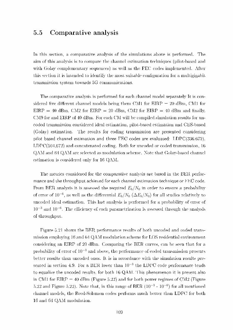
5.5 Comparative analysis
In this section, a comparative analysis of the simulations above is performed. The
aim of this analysis is to compare the channel estimation techniques (pilot-based and
with Golay complementary sequences) as well as the FEC codes implemented. After
this section it is intended to identify the most suitable conguration for a multigigabit
transmission system towards 5G communications.
The comparative analysis is performed for each channel model separately It is con-
sidered ve dierent channel models being them CM1 for EIRP = 20 dBm, CM1 for
EIRP = 40 dBm, CM2 for EIRP = 20 dBm, CM2 for EIRP = 40 dBm and nally,
CM9 for and EIRP of 40 dBm. For each CM will be compiled simulation results for un-
coded transmission considered ideal estimation, pilot-based estimation and CES-based
(Golay) estimation. The results for coding transmission are presented considering
pilot-based channel estimation and three FEC codes are evaluated: LDPC(336,672),
LDPC(504,672) and concatenated coding. Both for uncoded or coded transmission, 16
QAM and 64 QAM are selected as modulation scheme. Note that Golay-based channel
estimation is considered only for 16 QAM.
The metrics considered for the comparative analysis are based in the BER perfor-
mance and the throughput achieved for each channel estimation technique or FEC code.
From BER analysis it is assessed the required Eb/N0 in order to ensure a probability
of error of 10−6, as well as the dierential Eb/N0 (∆Eb/N0) for all studies relatively to
uncoded ideal estimation. This last analysis is performed for a probability of error of
10−3 and 10−6. The eciency of each parametrization is assessed through the analysis
of throughput.
Figure 5.21 shows the BER performance results of both uncoded and coded trans-
mission employing 16 and 64 QAM modulation scheme for LOS residential environment
considering an EIRP of 20 dBm. Comparing the BER curves, can be seen that for a
probability of error of 10−3 and above, the performance of coded transmission presents
better results than uncoded ones. It is in accordance with the simulation results pre-
sented in section 4.9. For a BER lower than 10−3 the LDPC code performance tends
to equalize the uncoded results, for both 16 QAM. This phenomenon it is present also
in CM1 for EIRP = 40 dBm (Figure 5.22) and for both power regimes of CM2 (Figure
5.22 and Figure 5.22). Note that, in this range of BER (10−3 - 10−6) for all mentioned
channel models, the Reed-Solomon codes performs much better than LDPC for both
16 and 64 QAM modulation.
109
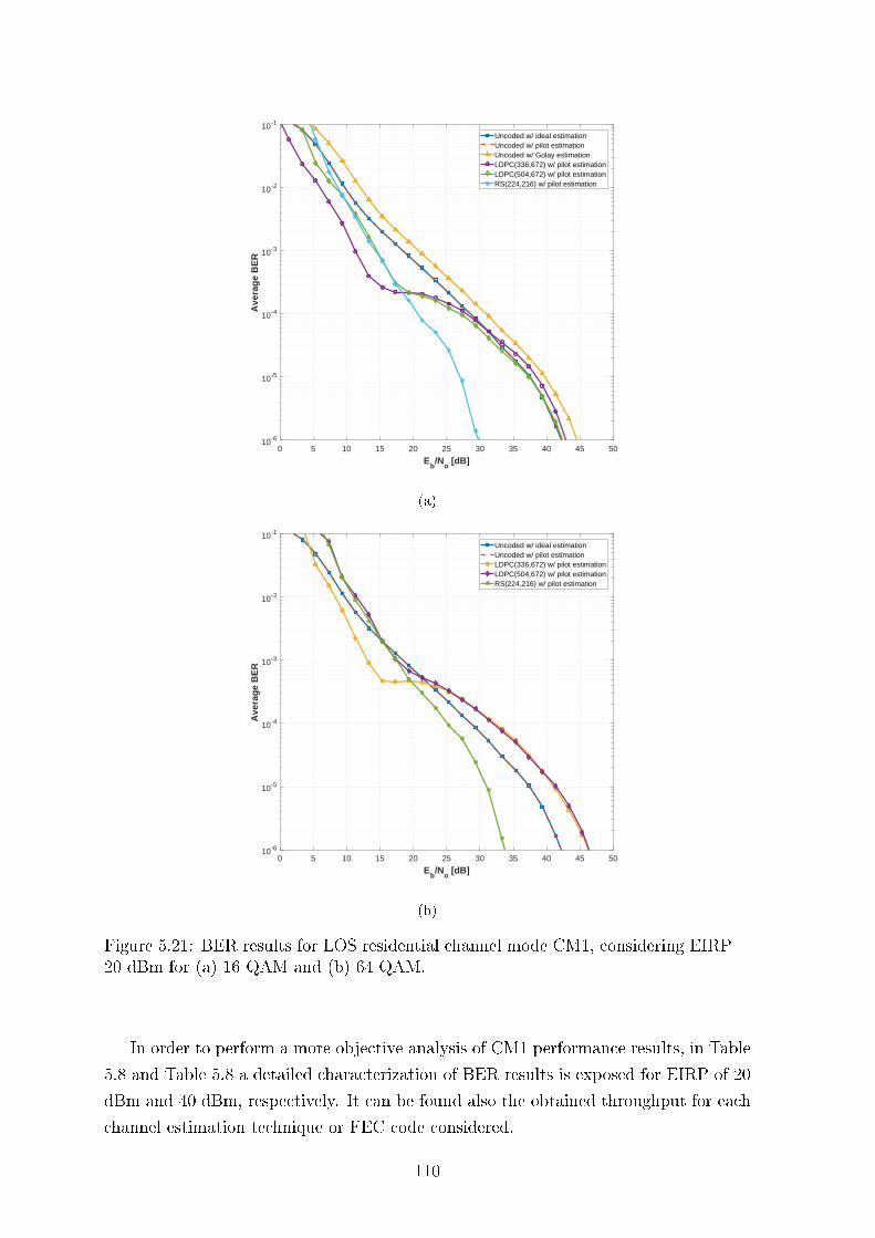
0 5 10 15 20 25 30 35 40 45 50
Eb/N
o [dB]
10-6
10-5
10-4
10-3
10-2
10-1
Ave
rag
e B
ER
Uncoded w/ ideal estimationUncoded w/ pilot estimationUncoded w/ Golay estimationLDPC(336,672) w/ pilot estimationLDPC(504,672) w/ pilot estimationRS(224,216) w/ pilot estimation
(a)
0 5 10 15 20 25 30 35 40 45 50
Eb/N
o [dB]
10-6
10-5
10-4
10-3
10-2
10-1
Ave
rag
e B
ER
Uncoded w/ ideal estimationUncoded w/ pilot estimationLDPC(336,672) w/ pilot estimationLDPC(504,672) w/ pilot estimationRS(224,216) w/ pilot estimation
(b)
Figure 5.21: BER results for LOS residential channel mode CM1, considering EIRP =20 dBm for (a) 16 QAM and (b) 64 QAM.
In order to perform a more objective analysis of CM1 performance results, in Table
5.8 and Table 5.8 a detailed characterization of BER results is exposed for EIRP of 20
dBm and 40 dBm, respectively. It can be found also the obtained throughput for each
channel estimation technique or FEC code considered.
110
Table 5.8: Simulation results for LOS residential channel mode CM1 for EIRP = 20dBm.
Modulation Parametrization Eb/N0 ∆Eb/N0 (dB) Throughput
(dB) @BER=10−3 @BER=10−6 (Mbps)
16 QAM
Uncoded Ideal 42 N/A N/A 6205
Uncoded Pilot 42 0 0 6186
Uncoded Golay 45 2.0 3 6129
LDPC(336,672) 43 -6.0 1 3093
LDPC(504,672) 42.5 -4.0 0.5 4639
RS(224,216) 29 -4.2 -12 3976
64 QAM
Uncoded Ideal 42 N/A N/A 12411
Uncoded Pilot 42 0 0 12373
LDPC(336,672) 46.5 -5.5 4.5 6186
LDPC(504,672) 46.5 -1 4.5 9279
RS(224,216) 34 -1 -8 7953
Analyzing both table results, it is clear the change on BER performance before and
after a probability of error of 10−3. The ∆Eb/N0 parameter shows that, considering a
BER of 1 in 1 million, only Reed-Solomon stands out in terms of performance when
compared with uncoded transmission. On the other hand, if it is admitted a higher
BER in the wireless system, then LDPC(336,672) codes outperforms RS.
111
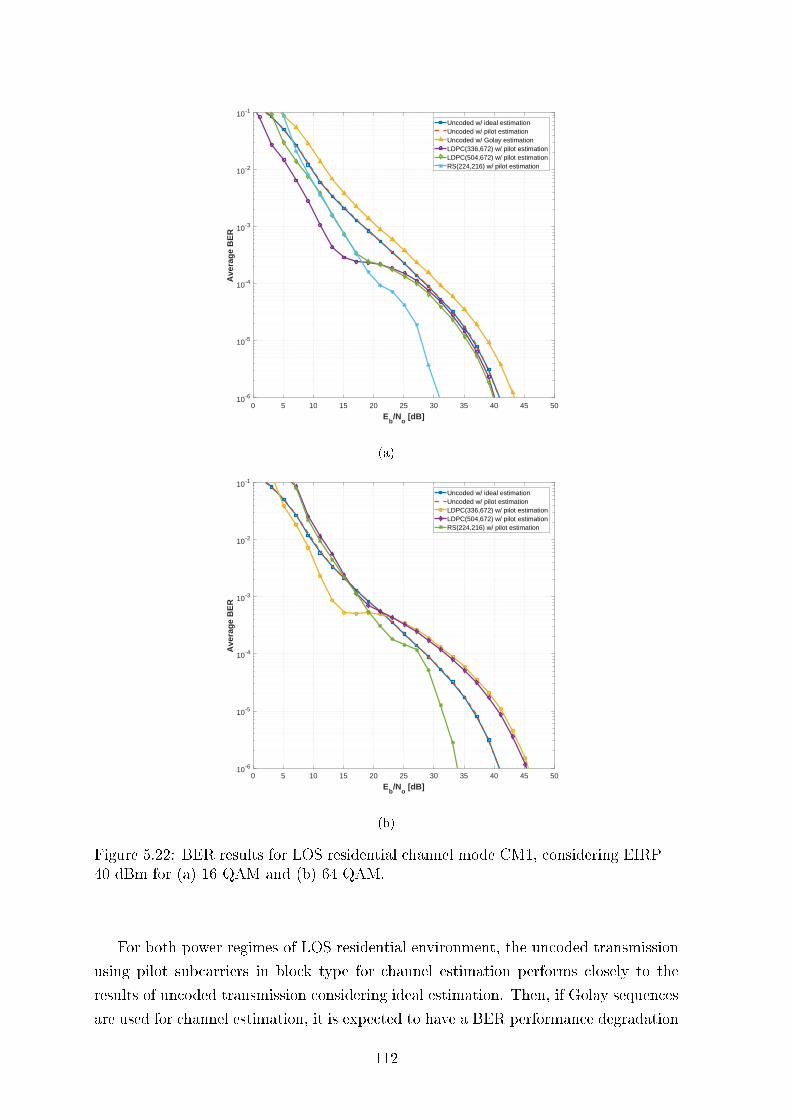
0 5 10 15 20 25 30 35 40 45 50
Eb/N
o [dB]
10-6
10-5
10-4
10-3
10-2
10-1
Ave
rag
e B
ER
Uncoded w/ ideal estimationUncoded w/ pilot estimationUncoded w/ Golay estimationLDPC(336,672) w/ pilot estimationLDPC(504,672) w/ pilot estimationRS(224,216) w/ pilot estimation
(a)
0 5 10 15 20 25 30 35 40 45 50
Eb/N
o [dB]
10-6
10-5
10-4
10-3
10-2
10-1
Ave
rag
e B
ER
Uncoded w/ ideal estimationUncoded w/ pilot estimationLDPC(336,672) w/ pilot estimationLDPC(504,672) w/ pilot estimationRS(224,216) w/ pilot estimation
(b)
Figure 5.22: BER results for LOS residential channel mode CM1, considering EIRP =40 dBm for (a) 16 QAM and (b) 64 QAM.
For both power regimes of LOS residential environment, the uncoded transmission
using pilot subcarriers in block type for channel estimation performs closely to the
results of uncoded transmission considering ideal estimation. Then, if Golay sequences
are used for channel estimation, it is expected to have a BER performance degradation
112
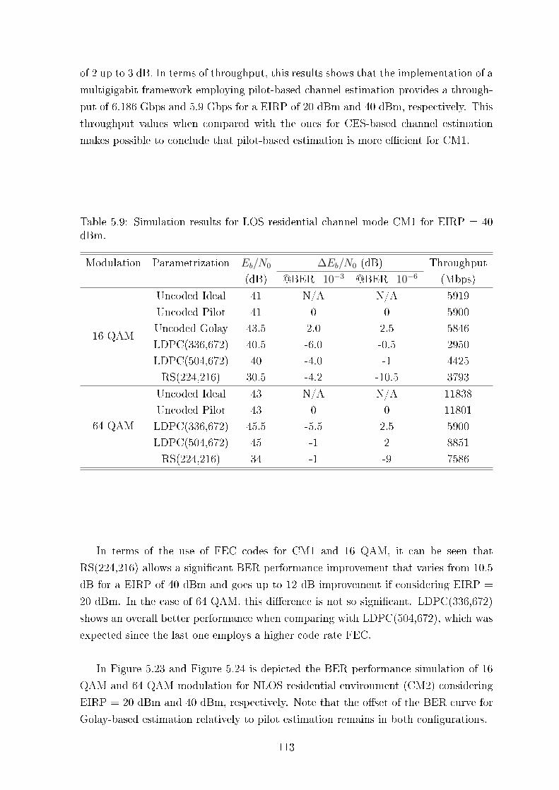
of 2 up to 3 dB. In terms of throughput, this results shows that the implementation of a
multigigabit framework employing pilot-based channel estimation provides a through-
put of 6.186 Gbps and 5.9 Gbps for a EIRP of 20 dBm and 40 dBm, respectively. This
throughput values when compared with the ones for CES-based channel estimation
makes possible to conclude that pilot-based estimation is more ecient for CM1.
Table 5.9: Simulation results for LOS residential channel mode CM1 for EIRP = 40dBm.
Modulation Parametrization Eb/N0 ∆Eb/N0 (dB) Throughput
(dB) @BER=10−3 @BER=10−6 (Mbps)
16 QAM
Uncoded Ideal 41 N/A N/A 5919
Uncoded Pilot 41 0 0 5900
Uncoded Golay 43.5 2.0 2.5 5846
LDPC(336,672) 40.5 -6.0 -0.5 2950
LDPC(504,672) 40 -4.0 -1 4425
RS(224,216) 30.5 -4.2 -10.5 3793
64 QAM
Uncoded Ideal 43 N/A N/A 11838
Uncoded Pilot 43 0 0 11801
LDPC(336,672) 45.5 -5.5 2.5 5900
LDPC(504,672) 45 -1 2 8851
RS(224,216) 34 -1 -9 7586
In terms of the use of FEC codes for CM1 and 16 QAM, it can be seen that
RS(224,216) allows a signicant BER performance improvement that varies from 10.5
dB for a EIRP of 40 dBm and goes up to 12 dB improvement if considering EIRP =
20 dBm. In the case of 64 QAM. this dierence is not so signicant. LDPC(336,672)
shows an overall better performance when comparing with LDPC(504,672), which was
expected since the last one employs a higher code rate FEC.
In Figure 5.23 and Figure 5.24 is depicted the BER performance simulation of 16
QAM and 64 QAM modulation for NLOS residential environment (CM2) considering
EIRP = 20 dBm and 40 dBm, respectively. Note that the oset of the BER curve for
Golay-based estimation relatively to pilot estimation remains in both congurations.
113
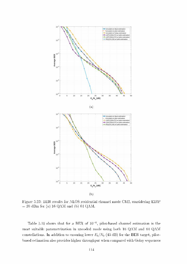
0 5 10 15 20 25 30 35 40 45 50
Eb/N
o [dB]
10-6
10-5
10-4
10-3
10-2
10-1
Ave
rag
e B
ER
Uncoded w/ ideal estimationUncoded w/ pilot estimationUncoded w/ Golay estimationLDPC(336,672) w/ pilot estimationLDPC(504,672) w/ pilot estimationRS(224,216) w/ pilot estimation
(a)
0 5 10 15 20 25 30 35 40 45 50
Eb/N
o [dB]
10-6
10-5
10-4
10-3
10-2
10-1
Ave
rag
e B
ER
Uncoded w/ ideal estimationUncoded w/ pilot estimationLDPC(336,672) w/ pilot estimationLDPC(504,672) w/ pilot estimationRS(224,216) w/ pilot estimation
(b)
Figure 5.23: BER results for NLOS residential channel mode CM2, considering EIRP= 20 dBm for (a) 16 QAM and (b) 64 QAM.
Table 5.10 shows that for a BER of 10−6, pilot-based channel estimation is the
most suitable parametrization in uncoded mode using both 16 QAM and 64 QAM
constellations. In addition to ensuring lower Eb/N0 (43 dB) for the BER target, pilot-
based estimation also provides higher throughput when compared with Golay sequences
114
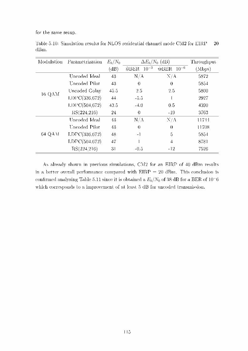
for the same setup.
Table 5.10: Simulation results for NLOS residential channel mode CM2 for EIRP = 20dBm.
Modulation Parametrization Eb/N0 ∆Eb/N0 (dB) Throughput
(dB) @BER=10−3 @BER=10−6 (Mbps)
16 QAM
Uncoded Ideal 43 N/A N/A 5872
Uncoded Pilot 43 0 0 5854
Uncoded Golay 45.5 2.5 2.5 5800
LDPC(336,672) 44 -5.5 1 2927
LDPC(504,672) 43.5 -4.0 0.5 4390
RS(224,216) 24 0 -19 3763
64 QAM
Uncoded Ideal 43 N/A N/A 11744
Uncoded Pilot 43 0 0 11708
LDPC(336,672) 48 -1 5 5854
LDPC(504,672) 47 1 4 8781
RS(224,216) 31 -0.5 -12 7526
As already shown in previous simulations, CM2 for an EIRP of 40 dBm results
in a better overall performance compared with EIRP = 20 dBm. This conclusion is
conrmed analyzing Table 5.11 since it is obtained a Eb/N0 of 38 dB for a BER of 10−6
which corresponds to a improvement of at least 5 dB for uncoded transmission.
115
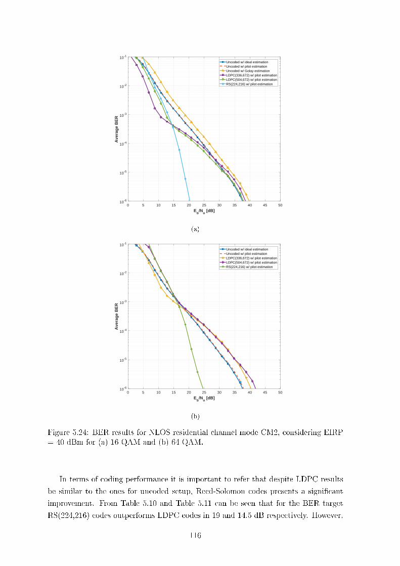
0 5 10 15 20 25 30 35 40 45 50
Eb/N
o [dB]
10-6
10-5
10-4
10-3
10-2
10-1
Ave
rag
e B
ER
Uncoded w/ ideal estimationUncoded w/ pilot estimationUncoded w/ Golay estimationLDPC(336,672) w/ pilot estimationLDPC(504,672) w/ pilot estimationRS(224,216) w/ pilot estimation
(a)
0 5 10 15 20 25 30 35 40 45 50
Eb/N
o [dB]
10-6
10-5
10-4
10-3
10-2
10-1
Ave
rag
e B
ER
Uncoded w/ ideal estimationUncoded w/ pilot estimationLDPC(336,672) w/ pilot estimationLDPC(504,672) w/ pilot estimationRS(224,216) w/ pilot estimation
(b)
Figure 5.24: BER results for NLOS residential channel mode CM2, considering EIRP= 40 dBm for (a) 16 QAM and (b) 64 QAM.
In terms of coding performance it is important to refer that despite LDPC results
be similar to the ones for uncoded setup, Reed-Solomon codes presents a signicant
improvement. From Table 5.10 and Table 5.11 can be seen that for the BER target
RS(224,216) codes outperforms LDPC codes in 19 and 14.5 dB respectively. However,
116
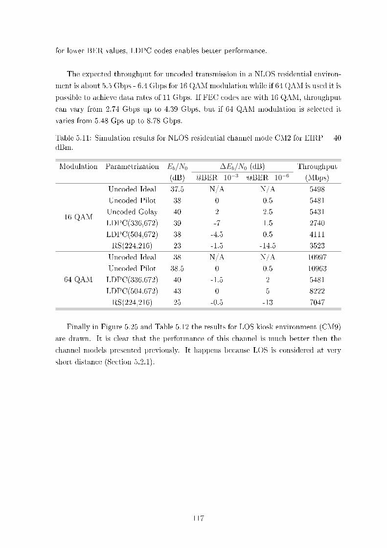
for lower BER values, LDPC codes enables better performance.
The expected throughput for uncoded transmission in a NLOS residential environ-
ment is about 5.5 Gbps - 6.4 Gbps for 16 QAM modulation while if 64 QAM is used it is
possible to achieve data rates of 11 Gbps. If FEC codes are with 16 QAM, throughput
can vary from 2.74 Gbps up to 4.39 Gbps, but if 64 QAM modulation is selected it
varies from 5.48 Gps up to 8.78 Gbps.
Table 5.11: Simulation results for NLOS residential channel mode CM2 for EIRP = 40dBm.
Modulation Parametrization Eb/N0 ∆Eb/N0 (dB) Throughput
(dB) @BER=10−3 @BER=10−6 (Mbps)
16 QAM
Uncoded Ideal 37.5 N/A N/A 5498
Uncoded Pilot 38 0 0.5 5481
Uncoded Golay 40 2 2.5 5431
LDPC(336,672) 39 -7 1.5 2740
LDPC(504,672) 38 -4.5 0.5 4111
RS(224,216) 23 -1.5 -14.5 3523
64 QAM
Uncoded Ideal 38 N/A N/A 10997
Uncoded Pilot 38.5 0 0.5 10963
LDPC(336,672) 40 -1.5 2 5481
LDPC(504,672) 43 0 5 8222
RS(224,216) 25 -0.5 -13 7047
Finally in Figure 5.25 and Table 5.12 the results for LOS kiosk environment (CM9)
are drawn. It is clear that the performance of this channel is much better then the
channel models presented previously. It happens because LOS is considered at very
short distance (Section 5.2.1).
117
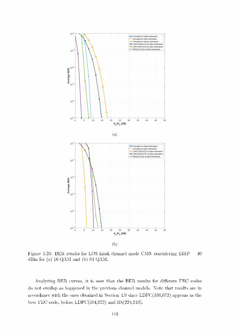
0 5 10 15 20 25 30 35 40 45 50
Eb/N
o [dB]
10-6
10-5
10-4
10-3
10-2
10-1
Ave
rag
e B
ER
Uncoded w/ ideal estimationUncoded w/ pilot estimationUncoded w/ Golay estimationLDPC(336,672) w/ pilot estimationLDPC(504,672) w/ pilot estimationRS(224,216) w/ pilot estimation
(a)
0 5 10 15 20 25 30 35 40 45 50
Eb/N
o [dB]
10-6
10-5
10-4
10-3
10-2
10-1
Ave
rag
e B
ER
Uncoded w/ ideal estimationUncoded w/ pilot estimationLDPC(336,672) w/ pilot estimationLDPC(504,672) w/ pilot estimationRS(224,216) w/ pilot estimation
(b)
Figure 5.25: BER results for LOS kiosk channel mode CM9, considering EIRP = 40dBm for (a) 16 QAM and (b) 64 QAM.
Analyzing BER curves, it is seen that the BER results for dierent FEC codes
do not overlap as happened in the previous channel models. Note that results are in
accordance with the ones obtained in Section 4.9 since LDPC(336,672) appears as the
best FEC code, before LDPC(504,672) and RS(224,216).
118
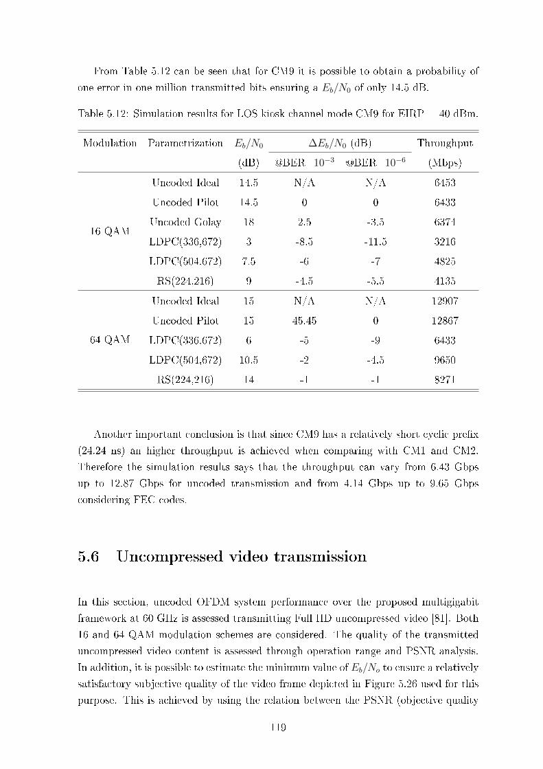
From Table 5.12 can be seen that for CM9 it is possible to obtain a probability of
one error in one million transmitted bits ensuring a Eb/N0 of only 14.5 dB.
Table 5.12: Simulation results for LOS kiosk channel mode CM9 for EIRP = 40 dBm.
Modulation Parametrization Eb/N0 ∆Eb/N0 (dB) Throughput
(dB) @BER=10−3 @BER=10−6 (Mbps)
16 QAM
Uncoded Ideal 14.5 N/A N/A 6453
Uncoded Pilot 14.5 0 0 6433
Uncoded Golay 18 2.5 -3.5 6374
LDPC(336,672) 3 -8.5 -11.5 3216
LDPC(504,672) 7.5 -6 -7 4825
RS(224,216) 9 -4.5 -5.5 4135
64 QAM
Uncoded Ideal 15 N/A N/A 12907
Uncoded Pilot 15 45.45 0 12867
LDPC(336,672) 6 -5 -9 6433
LDPC(504,672) 10.5 -2 -4.5 9650
RS(224,216) 14 -1 -1 8271
Another important conclusion is that since CM9 has a relatively short cyclic prex
(24.24 ns) an higher throughput is achieved when comparing with CM1 and CM2.
Therefore the simulation results says that the throughput can vary from 6.43 Gbps
up to 12.87 Gbps for uncoded transmission and from 4.14 Gbps up to 9.65 Gbps
considering FEC codes.
5.6 Uncompressed video transmission
In this section, uncoded OFDM system performance over the proposed multigigabit
framework at 60 GHz is assessed transmitting Full HD uncompressed video [81]. Both
16 and 64 QAM modulation schemes are considered. The quality of the transmitted
uncompressed video content is assessed through operation range and PSNR analysis.
In addition, it is possible to estimate the minimum value of Eb/No to ensure a relatively
satisfactory subjective quality of the video frame depicted in Figure 5.26 used for this
purpose. This is achieved by using the relation between the PSNR (objective quality
119
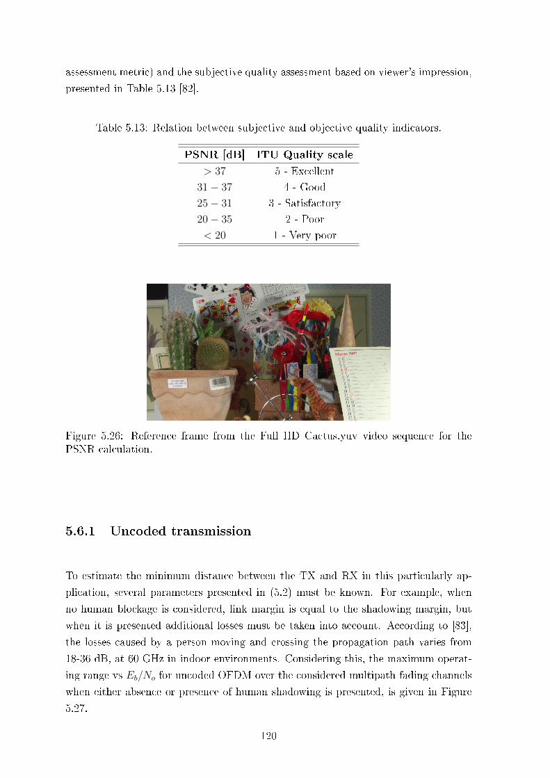
assessment metric) and the subjective quality assessment based on viewer's impression,
presented in Table 5.13 [82].
Table 5.13: Relation between subjective and objective quality indicators.
PSNR [dB] ITU Quality scale
> 37 5 - Excellent
31− 37 4 - Good
25− 31 3 - Satisfactory
20− 35 2 - Poor
< 20 1 - Very poor
Figure 5.26: Reference frame from the Full HD Cactus.yuv video sequence for thePSNR calculation.
5.6.1 Uncoded transmission
To estimate the minimum distance between the TX and RX in this particularly ap-
plication, several parameters presented in (5.2) must be known. For example, when
no human blockage is considered, link margin is equal to the shadowing margin, but
when it is presented additional losses must be taken into account. According to [83],
the losses caused by a person moving and crossing the propagation path varies from
18-36 dB, at 60 GHz in indoor environments. Considering this, the maximum operat-
ing range vs Eb/No for uncoded OFDM over the considered multipath fading channels
when either absence or presence of human shadowing is presented, is given in Figure
5.27.
120
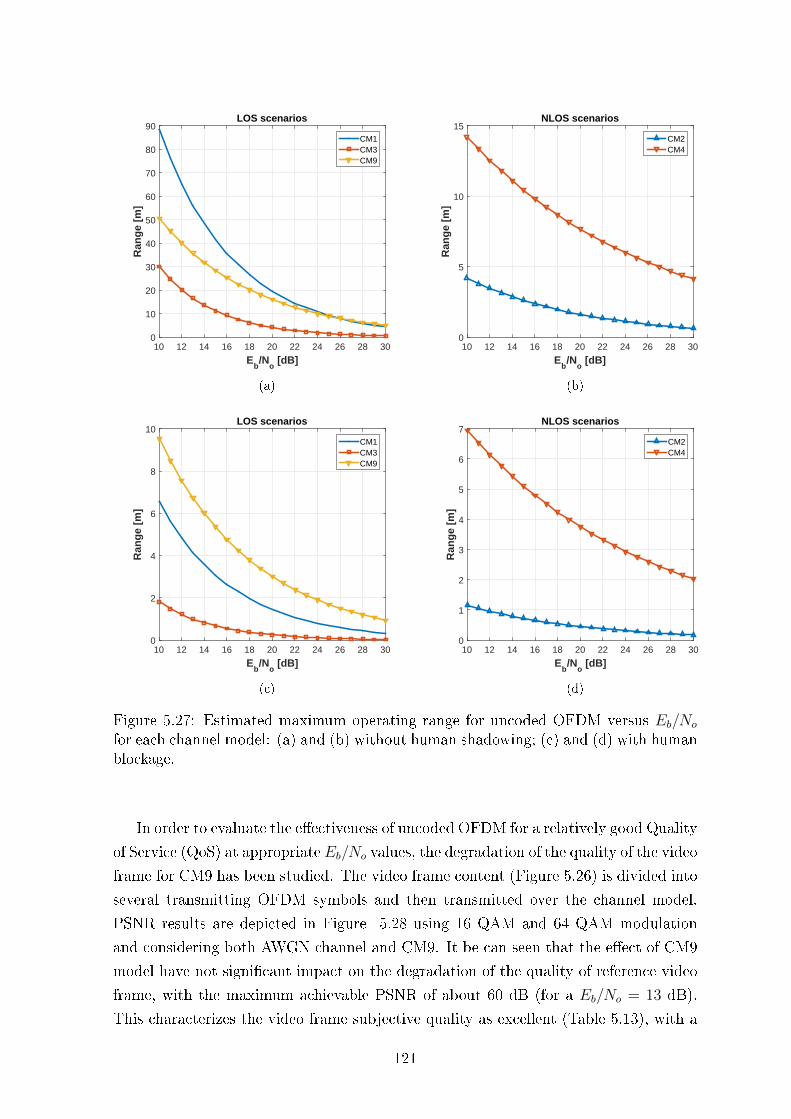
Eb/N
o [dB]
10 12 14 16 18 20 22 24 26 28 30
Ran
ge
[m]
0
10
20
30
40
50
60
70
80
90LOS scenarios
CM1CM3CM9
(a)
Eb/N
o [dB]
10 12 14 16 18 20 22 24 26 28 30
Ran
ge
[m]
0
5
10
15NLOS scenarios
CM2CM4
(b)
Eb/N
o [dB]
10 12 14 16 18 20 22 24 26 28 30
Ran
ge
[m]
0
2
4
6
8
10LOS scenarios
CM1CM3CM9
(c)
Eb/N
o [dB]
10 12 14 16 18 20 22 24 26 28 30
Ran
ge
[m]
0
1
2
3
4
5
6
7NLOS scenarios
CM2CM4
(d)
Figure 5.27: Estimated maximum operating range for uncoded OFDM versus Eb/No
for each channel model: (a) and (b) without human shadowing; (c) and (d) with humanblockage.
In order to evaluate the eectiveness of uncoded OFDM for a relatively good Quality
of Service (QoS) at appropriate Eb/No values, the degradation of the quality of the video
frame for CM9 has been studied. The video frame content (Figure 5.26) is divided into
several transmitting OFDM symbols and then transmitted over the channel model.
PSNR results are depicted in Figure 5.28 using 16 QAM and 64 QAM modulation
and considering both AWGN channel and CM9. It be can seen that the eect of CM9
model have not signicant impact on the degradation of the quality of reference video
frame, with the maximum achievable PSNR of about 60 dB (for a Eb/No = 13 dB).
This characterizes the video frame subjective quality as excellent (Table 5.13), with a
121
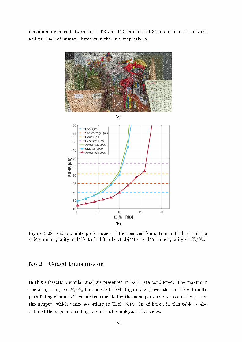
maximum distance between both TX and RX antennas of 34 m and 7 m, for absence
and presence of human obstacles in the link, respectively.
(a)
0 5 10 15 20
Eb/N
o [dB]
10
15
20
25
30
35
40
45
50
55
60
PS
NR
[d
B]
Poor QoSSatisfactory QoSGood QosExcellent QosAWGN 16 QAMCM9 16 QAMAWGN 64 QAM
(b)
Figure 5.28: Video quality performance of the received frame transmitted: a) subjectvideo frame quality at PSNR of 14.01 dB b) objective video frame quality vs Eb/No.
5.6.2 Coded transmission
In this subsection, similar analysis presented in 5.6.1, are conducted. The maximum
operating range vs Eb/No for coded OFDM (Figure 5.29) over the considered multi-
path fading channels is calculated considering the same parameters, except the system
throughput, which varies according to Table 5.14. In addition, in this table is also
detailed the type and coding rate of each employed FEC codes.
122
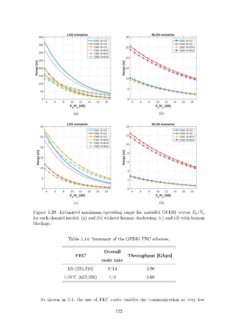
Eb/N
o [dB]
4 6 8 10 12 14 16 18
Ran
ge
[m]
0
50
100
150
200
250
300
350
400LOS scenarios
CM1, R=1/2CM3, R=1/2CM9, R=1/2CM1, R=9/14CM3, R=9/14CM9, R=9/14
(a)
Eb/N
o [dB]
4 6 8 10 12 14 16 18
Ran
ge
[m]
0
5
10
15
20
25
30NLOS scenarios
CM2, R=1/2CM4, R=1/2CM2, R=9/14CM4, R=9/14
(b)
Eb/N
o [dB]
4 6 8 10 12 14 16 18
Ran
ge
[m]
0
5
10
15
20
25
30LOS scenarios
CM1, R=1/2CM3, R=1/2CM9, R=1/2CM1, R=9/14CM3, R=9/14CM9, R=9/14
(c)
Eb/N
o [dB]
4 6 8 10 12 14 16 18
Ran
ge
[m]
0
2
4
6
8
10
12
14NLOS scenarios
CM2, R=1/2CM4, R=1/2CM2, R=9/14CM4, R=9/14
(d)
Figure 5.29: Estimated maximum operating range for uncoded OFDM versus Eb/No
for each channel model: (a) and (b) without human shadowing; (c) and (d) with humanblockage.
Table 5.14: Summary of the OFDM FEC schemes.
FECOverall
code rateThroughput [Gbps]
RS (224,216) 9/14 3.96
LDPC (672,336) 1/2 3.08
As shown in 5.4, the use of FEC codes enables the communication at very low
123

Signal-to-Noise Ratios (SNRs). BER target is achieved for Eb/No values of 10 dB
and 3.6 dB for RS and LDPC coding, respectively. This allows the TX and RX to
be antennas to be apart of 150 m and 28.2 m (this one in the presence of human
shadowing) considering a coding rate of 1/2. Similarly, when a coding rate of 9/14 is
used, both distances are 133.2 m and 25 m, which means that channel coding make the
system more robust against noise and thus its operating range is signicantly increased.
For example, when LDPC coding is employed this distance increases 121.5 m and 22.8
m, for absence and presence of disturbances in the transmission medium, relatively to
the uncoded OFDM system.
5.7 Summary
The fth chapter reports the performance evaluation of the proposed framework over
indoor multipath fading channels and considering the IEEE 802.15.3c standard as ref-
erence. First, the study scenarios for the performance assessment are presented. It is
considered the indoor environments suggested by TG3c group and the corresponding
link budget and mobility considerations. The performance assessment is divided in two
main groups: uncoded OFDM system assessment and coded OFDM system assessment.
In the rst group, a parametric study is reported in order to nd the most suitable
cyclic prex length for each channel model. Then, the performance results based on
channel estimation using pilot subcarriers and Golay sequences are presented. The sec-
ond group shows the simulation results of a transmission employing FEC codes. The
chapter ends with a comparative analysis of the main results obtained previously.
124
Chapter 6
Conclusions
6.1 Summary
Chapter 2 presented a review of the main contributions in the literature referring multi-
gigabit prototyping testbeds addressed to 5 G requirements. After a quick description of
each project, Table 2.1 compiles the main characteristics of each testbed. the high spec-
tral eciency is transversal to almost every project since MIMO techniques are used.
Among with the presented testbeds, spectral eciencies of 67.26 and 145.6 bit/s/Hz
can be obtained. Despite the good performance in terms of spectral eciency, non of
the projects is implemented in 60 GHz band, which could be even more protable, due
to high bandwidth available. In this Chapter, a overview of two standards operating
at 60 GHz is conducted, IEEE 802.11ad and IEEE 802.15.3c. These standards dene
several PHY layer modes in order to meet with dierent requirements. Since IEEE
802.15.3c was the rst standard addressing multigigabit data rates at 60 GHz, it is the
standard taken as reference in the work.
In Chapter 3, the theoretical fundamentals for the work are presented. First, a de-
tailed description of a OFDM system is conducted, as well as the analytic expressions
related to it. Next, the concepts related to multipath fading channels are introduced.
The fading channel is subdivided in large-scale fading eects and small-scale fading
eects and the parameters used to characterize these two categories of fading channel
response are detailed. In this Chapter the most commonly used channel coding ap-
proaches are presented and the theoretical aspects of channel estimation based on both
pilot subcarriers and Golay sequences and frequency domain equalization are discussed.
Chapter 4 aims to present the proposed simulation framework for multigigabit ap-
125
plications. Initially, the general block diagram of the framework is shown and the
overall operation is discussed. Then, each block of general block diagram is detailed.
This Chapter also addresses the performance evaluation metric considered for the work.
Finally, simulation results are conducted in order to validate the simulation framework.
Chapter 5 refers to performance evaluation of 60 GHz OFDM framework over indoor
multipath fading channels. The indoor multipath fading channels are obtained and
characterized according to the suggestions of TG3c group. After dening the channel
models considered for the performance evaluation, the framework is loaded with the
parameters of IEEE 802.15.3c. The performance assessment is divided in two main
groups: uncoded OFDM system assessment and coded OFDM system assessment.
The chapter ends with a comparative analysis of the main results obtained previously
from both uncoded and coded OFDM system assessments.
6.2 Main conclusions
This work presents a simulation framework for multigigabit applications based on
OFDM modulation at mmWave frequencies. The main goal of the framework is to
provide a modular simulation tool designed for high data rate application in order to
be easily adapted to a specic standard or technology, such as 5G. The presented frame-
work allows the employment of 16 QAM or 64 QAMmodulation scheme, and the length
of the cyclic prex extension is also congurable. In order to simulate a realistic multi-
path fading channel, the proposed framework allows the insertion of a channel impulse
response dened by the user. The channel estimation can be performed either using
pilot subcarriers or Golay sequence as channel estimation sequences. Independently of
the channel estimation technique selected, frequency domain equalization is available
through ZF approach or MMSE. The simulation framework also allows channel coding
techniques in order to provide a more robustness transmission and to improve the link
budget.
The performance assessment of the framework is based on IEEE 802.15.3c. From
the analysis of the performance indicators returned from the simulation framework, it
was concluded that the transmitted symbols were being aected by ISI, which means
that the cyclic prex suggested by the standard is not suitable for the channel models
considered. Thus, a parametric study was conducted in order to nd the CP length
that reduce ISI eect but does not compromise the spectral eciency of the system.
It was dened that a TCP = τmax is a good approach. Therefore, further simulations
126
considers the TCP proposed in the parametric study. Other simulations showed that
the pilot arrangement suggested by IEEE 802.15.3c does not provide the desired per-
formance since the channel models considered are highly frequency selective. Thus, it
was suggested the implementation of a block type pilot arrangement where the pilot
symbol transmission period is dependent on the coherence time of the channel.
In terms of comparative analysis of the dierent channel estimation approaches,
it is seen that pilot-based channel estimation in block type arrangement outperforms
Golay sequences transmission in terms of BER performance and throughput. It can
also be concluded that concatenated codes outperforms LDPC codes for high BER
levels, which does not happen for BER values of approximately 10−3. From these
analysis it is concluded that for uncoded transmissions, pilot-based is the most suitable
approach for channel estimation purposes and for coded transmissions, concatenated
codes, composed by Reed Solomon and convolutional codes, are suggested.
6.3 Further work
In this work, the implementation of a simulation framework for multigigabit applica-
tions at mmWave frequencies is proposed and described. Nevertheless, there are still
some topics that require further investigation work. Next, those topics are described
• Extension of the simulation framework in order to include RF impair-
ments. As refereed in Section 4.2, the performance of OFDM at mmWave is
severely aected by non-linearities of RF front-end. Thus, in order to compen-
sate these non-linearities, RF impairments, such as phase-noise, mixer IQ imbal-
ances, and power amplier non-linearities must be considered in the simulation
framework.
• Integration of the 5G PHY layer requirements in the framework. Due
to the scalability of the framework, once dened the standard responsible for
supporting 5G mobile communications, it will be possible to integrate the PHY
layer requirements in the proposed framework. It will be possible then, to rapidly
test and validate new techniques and/or methods.
• Hardware Prototyping of end-to-end multigigabit OFDM based for 5G
communications. Having a simulation platform able to test and evaluate new
techniques for the development of 5G communications, the implementation of a
127
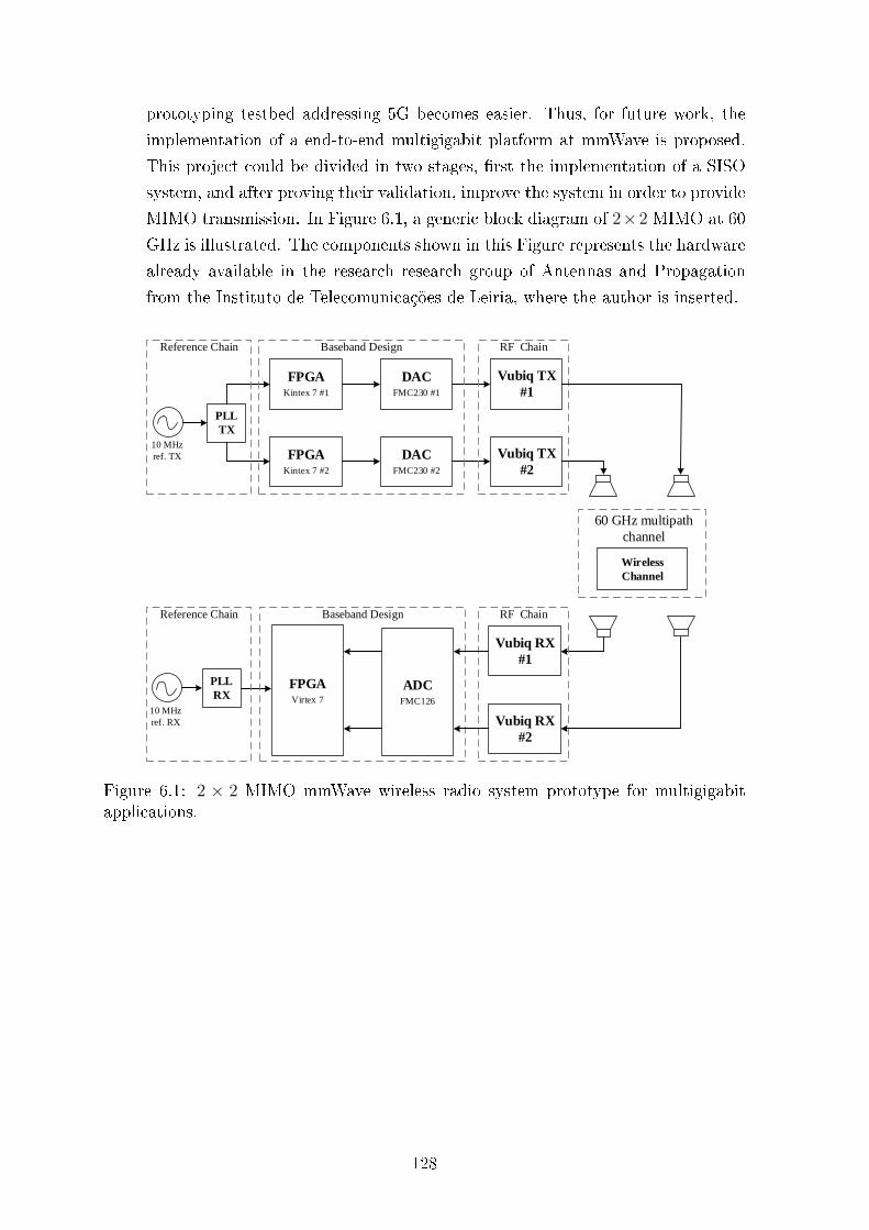
prototyping testbed addressing 5G becomes easier. Thus, for future work, the
implementation of a end-to-end multigigabit platform at mmWave is proposed.
This project could be divided in two stages, rst the implementation of a SISO
system, and after proving their validation, improve the system in order to provide
MIMO transmission. In Figure 6.1, a generic block diagram of 2×2 MIMO at 60
GHz is illustrated. The components shown in this Figure represents the hardware
already available in the research research group of Antennas and Propagation
from the Instituto de Telecomunicações de Leiria, where the author is inserted.
PLL
TX
FPGA Kintex 7 #1
FPGA Kintex 7 #2
DACFMC230 #1
DACFMC230 #2
Vubiq TX
#1
Vubiq TX
#2
10 MHz
ref. TX
Reference Chain Baseband Design RF Chain
Vubiq RX
#1
Vubiq RX
#2
RF Chain
Wireless
Channel
60 GHz multipath
channel
ADCFMC126
FPGA Virtex 7
Baseband Design
PLL
RX
Reference Chain
10 MHz
ref. RX
Figure 6.1: 2 × 2 MIMO mmWave wireless radio system prototype for multigigabitapplications.
128
Bibliography
[1] S.-K. Yong, P. Xia, and A. Valdes-Garcia, 60 GHz TECHNOLOGY FOR GBPS
WLAN AND WPAN. WILEY, 2011.
[2] 802.15.3c-2009 - Physical Layer (PHY) Specications for High Rate Wireless Per-
sonal Area Networks (WPANs) (IEEE 802.15.3c).
[3] T. Nitsche, C. Cordeiro, A. B. Flores, E. W. Knightly, E. Perahia, and J. C. Wid-
mer, IEEE 802.11ad: directional 60 GHz communication for multi-Gigabit-per-
second Wi-Fi [Invited Paper], IEEE Communications Magazine, vol. 52, pp. 132
141, December 2014.
[4] A. Younis, N. Abuzgaia, R. Mesleh, and H. Haas, Quadrature Spatial Modula-
tion for 5G Outdoor Millimeter-Wave Communications: Capacity Analysis, IEEE
Transactions on Wireless Communications, vol. PP, no. 99, pp. 11, 2017.
[5] A. S. Marcano and H. L. Christiansen, Performance of Non-Orthogonal Multi-
ple Access (NOMA) in mmWave wireless communications for 5G networks, in
2017 International Conference on Computing, Networking and Communications
(ICNC), pp. 969974, Jan 2017.
[6] R. V. Nee and R. Prasad, OFDM for Wireless Communications. Artech House
Publishers, 1999.
[7] M. Lei and Y. Huang, CFR and SNR Estimation Based on Complementary Golay
Sequences for Single-Carrier Block Transmission in 60-GHz WPAN, in IEEE
Wireless Communications and Networking Conference, 2009. WCNC 2009, pp. 1
5, Apr. 2009.
[8] P. Kumari, N. Gonzalez-Prelcic, and R. W. Heath, Investigating the IEEE
802.11ad Standard for Millimeter Wave Automotive Radar, in Vehicular Tech-
nology Conference (VTC Fall), 2015 IEEE 82nd, pp. 15, Sept 2015.
[9] W. C. Liu, F. C. Yeh, T. C. Wei, C. D. Chan, and S. J. Jou, A Digital Golay-
MPIC Time Domain Equalizer for SC/OFDM Dual-Modes at 60 GHz Band,
IEEE Transactions on Circuits and Systems I: Regular Papers, vol. 60, pp. 2730
2739, Oct 2013.
129
[10] W. C. Liu, T. C. Wei, Y. S. Huang, C. D. Chan, and S. J. Jou, All-Digital
Synchronization for SC/OFDM Mode of IEEE 802.15.3c and IEEE 802.11ad,
IEEE Transactions on Circuits and Systems I: Regular Papers, vol. 62, pp. 545
553, Feb 2015.
[11] C. F. Wu, W. C. Liu, C. C. Tsui, C. Y. Liu, M. S. Sie, and S. J. Jou, Golay-
Correlator Window-Based Noise Cancellation Equalization Technique for 60-GHz
Wireless OFDM/SC Receiver, IEEE Transactions on Very Large Scale Integra-
tion (VLSI) Systems, vol. PP, no. 99, pp. 111, 2016.
[12] L. Chen, G. Yue, X. Cheng, and S. Li, Time-domain frequency-dependent I/Q
imbalance compensation based on golay sequence, in 2014 IEEE 11th Consumer
Communications and Networking Conference (CCNC), pp. 531536, Jan 2014.
[13] A. E. Assaf, N. Kandil, N. Hakem, S. Aes, and P. Fortier, A study of 60 GHz
channel estimation techniques using pilot carriers in OFDM systems in a conned
area, in Wireless Communications in Unusual and Conned Areas (ICWCUCA),
2012 International Conference on, pp. 16, Aug 2012.
[14] B. Ye and Z. Zhang, Improved pilot design and channel estimation for 60GHz
OFDM based on IEEE 802.11.ad, in 2013 IEEE Wireless Communications and
Networking Conference (WCNC), pp. 41294133, April 2013.
[15] M. K. Ozdemir and H. Arslan, Channel Estimation for Wireless OFDM Systems,
IEEE Communications Surveys Tutorials, vol. 9, pp. 1848, Second 2007.
[16] L. Li, R. C. de Lamare, and A. G. Burr, Dynamic pilot allocation with channel
estimation in closed-loop multi-input-multi-output orthogonal frequency division
multiplexing systems, IET Communications, vol. 8, pp. 20172025, July 2014.
[17] P. Pakrooh, A. Amini, and F. Marvasti, OFDM pilot allocation for sparse channel
estimation, CoRR, vol. abs/1106.4507, 2011.
[18] W. S. H. Z. X. W. J. W. H. Zhang, Research on Channel Estimation Algorithm in
60GHz System Based on 802.15.3c Standard, Journal of Communications, vol. 9,
2014.
[19] J. C. Guey and A. Osseiran, Adaptive Pilot Allocation in Downlink OFDM, in
2008 IEEE Wireless Communications and Networking Conference, pp. 840845,
March 2008.
[20] L. U. Khan, S. A. Mahmud, G. M. Khan, M. H. Zafar, and M. Ashraf, Chan-
nel estimation based on Non-Equally Spaced Pilot allocation in OFDM system,
130
in Computer Science and Electronic Engineering Conference (CEEC), 2014 6th,
pp. 139143, Sept 2014.
[21] B. Rajarshi Banerjee and T. Rao, Pilot Design based Channel Estimation for
IEEE 802.11ad Wireless Communications at 60 GHz, in International Confer-
ence on Signal Processing, Embedded System and Communication Technologies
and their applications for Sustainable and Renewable Energy (ICSECSRE), 2014,
pp. 385391, April 2014.
[22] Su-Khiong Yong, TG3c Channel Modeling Sub-committee Final Report. Samsung
Advanced Institute of Technology, Mar. 2007.
[23] 5GNOW, 5GNOW: 5th Generation Non-Orthogonal Waveforms for Asyn-
chronous Signalling.
[24] I. T. U. (ITU), Minimum requirements related to technical performance for IMT-
2020 radio interface(s).
[25] M. Schellmann, Z. Zhao, H. Lin, P. Siohan, N. Rajatheva, V. Luecken, and
A. Ishaque, FBMC-based air interface for 5G mobile: Challenges and proposed so-
lutions, in 2014 9th International Conference on Cognitive Radio Oriented Wire-
less Networks and Communications (CROWNCOM), pp. 102107, June 2014.
[26] P. Guan, D. Wu, T. Tian, J. Zhou, X. Zhang, L. Gu, A. Benjebbour, M. Iwabuchi,
and Y. Kishiyama, 5G Field Trials - OFDM-based Waveforms and Mixed Nu-
merologies, IEEE Journal on Selected Areas in Communications, vol. PP, no. 99,
pp. 11, 2017.
[27] R. Mà c©ndez-Rial, C. Rusu, N. Gonzýlez-Prelcic, A. Alkhateeb, and R. W.
Heath, Hybrid MIMO Architectures for Millimeter Wave Communications: Phase
Shifters or Switches?, IEEE Access, vol. 4, pp. 247267, 2016.
[28] T. E. Bogale and L. B. Le, Beamforming for multiuser massive MIMO systems:
Digital versus hybrid analog-digital, in 2014 IEEE Global Communications Con-
ference, pp. 40664071, Dec 2014.
[29] C. Shepard, H. Yu, N. Anand, L. E. Li, T. Marzetta, R. Yang, and L. Zhong,
Argos: Practical Many-Antenna Base Stations, in MobiCom 12, Aug 2012.
[30] H. Y. Clayton Shepard and L. Zhong, ArgosV2: A Flexible Many-Antenna Re-
search Platform, in MobiCom 13, Sept 2013.
[31] WARP, WARP: Wireless Open Access Research Platform.
131
[32] J. Vieira, S. Malkowsky, K. Nieman, Z. Miers, N. Kundargi, L. Liu, I. Wong,
V. Owall, O. Edfors, and F. Tufvesson, A exible 100-antenna testbed for Massive
MIMO, in 2014 IEEE Globecom Workshops (GC Wkshps), pp. 287293, Dec 2014.
[33] H. Suzuki, R. Kendall, K. Anderson, A. Grancea, D. Humphrey, J. Pathikulangara,
K. Bengston, J. Matthews, and C. Russell, Highly spectrally ecient Ngara Rural
Wireless Broadband Access Demonstrator, in 2012 International Symposium on
Communications and Information Technologies (ISCIT), pp. 914919, Oct 2012.
[34] W. Zhang, J. Xiang, Y. N. R. Li, Y. Wang, Y. Chen, P. Geng, and Z. Lu, Field
trial and future enhancements for TDD massive MIMO networks, in 2015 IEEE
26th Annual International Symposium on Personal, Indoor, and Mobile Radio
Communications (PIMRC), pp. 23392343, Aug 2015.
[35] Samsung, Samsung takes rst 5g steps with advanced antenna.
[36] P. Harris, W. B. Hasan, S. Malkowsky, J. Vieira, S. Zhang, M. Beach, L. Liu,
E. Mellios, A. Nix, S. Armour, A. Doufexi, K. Nieman, and N. Kundargi, Serving
22 Users in Real-Time with a 128-Antenna Massive MIMO Testbed, in 2016
IEEE International Workshop on Signal Processing Systems (SiPS), pp. 266272,
Oct 2016.
[37] University of Bristol, Communication Systems and Networks Research Group.
[38] A. Tecnhologies, Wireless LAN at 60 GHz - IEEE 802.11ad Explained, IEEE
Communications Magazine, May 2013.
[39] A. Sadri, Summary of the Usage Models for 802.15.3c. IEEE 802.15-06-0369-09-
003c, 2006.
[40] S.-K. Yong, TG3c Channel Modeling Sub-committee Final Report. IEEE 802.15-
07-0584-01-003c, 2007.
[41] Z. L. J. W. M. A. R. Tuncer Baykas, Chin-Sean Sum and H. Harada, IEEE
802.15.3c: The First IEEE Wireless Standard for Data Rates over 1 Gb/s. IEEE
Communications Magazine, 2011.
[42] A. F.Molisch, Wireless Communications. WILEY, 2011.
[43] W. Yong Soo Cho, Jaekwon Kim and Chung G. Kang, MIMO-OFDM Wireless
Communications with MATLAB. Wiley.
[44] C. L. Henrik Schulze, Theory and Applications of OFDM and CDMA. WILEY.
132
[45] T. S. Rappaport, Wireless Communications: Principles and Practice. Prentice
Hall, 2 edition ed., Jan. 2002.
[46] B. Sklar, Digital Communications: Fundamentaals and Applications. Prentice
Hall, 2 edition ed., 2002.
[47] H. Abdulkarim, Comparison of Proposals for the Future Aeronautical Communi-
cation System LDACS.
[48] C. Anderson and T. Rapapport, In-building wideband partition loss measure-
ments at 2.5 and 60 GHz, IEEE transactions on Wireless Communications, vol. 3,
pp. 922928, 2004.
[49] H. Harada, R. Funada, H. Sawada, and S. Kato, CM MATLAB Release Support
Document. Mar. 2007.
[50] P. F. M. Smulders, Statistical Characterization of 60-GHz Indoor Radio Chan-
nels, 2009.
[51] A. Saleh and R. Valenzuela, A Statistical Model for Indoor Multipath Propaga-
tion, IEEE Journal on Selected Areas in Communications, vol. 5, pp. 128137,
Feb. 1987.
[52] Q. Spencer, B. Jes, M. Jensen, and A. Swindlehurst, Modeling the statistical
time and angle of arrival characteristics of an indoor multipath channel, IEEE
Journal on Selected Areas in Communications, vol. 18, pp. 347360, Mar. 2000.
[53] J. G. Proakis and M. Salehi, Digital Communications. McGraw-Hill, 5 edition ed.,
2008.
[54] A. Khli and R. Bouallegue, Performance Analysis of LS and LMMSE Channel
Estimation Techniques for LTE Downlink Systems, vol. 58, no. 5, pp. 141149,
2011.
[55] B. Ye and Z. Zhang, Improved pilot design and channel estimation for 60GHz
OFDM based on IEEE 802.11.ad, in 2013 IEEE Wireless Communications and
Networking Conference (WCNC), pp. 41294133, April 2013.
[56] L. Kewen and XingKe, Research of MMSE and LS channel estimation in OFDM
systems, in The 2nd International Conference on Information Science and Engi-
neering, pp. 23082311, Dec 2010.
[57] S. Coleri, M. Ergen, A. Puri, and A. Bahai, Channel estimation techniques based
on pilot arrangement in OFDM systems, IEEE Transactions on Broadcasting,
vol. 48, pp. 223229, Sep 2002.
133
[58] F. Wang, Pilot-based channel estimation in OFDM system.
[59] M. Golay, Complementary series, IRE Transactions on Information Theory,
vol. 7, pp. 8287, April 1961.
[60] B. M. Popovic, Ecient Golay correlator, IEE Electron. Lett, vol. 35, pp. 1427
1428, Aug 1999.
[61] M. Lei, I. Lakkis, H. Harada, and S. Kato, MMSE-FDE Based on Estimated
SNR for Single-Carrier Block Transmission (SCBT) in Multi-Gbps WPAN (IEEE
802.15.3c), in IEEE International Conference on Communications Workshops,
2008. ICC Workshops '08, pp. 5256, May 2008.
[62] MathWorks, Simulink.
[63] MathWorks, DSP System Toolbox.
[64] MathWorks, Sample- and Frame-Based Concepts.
[65] R. Kimura, R. Funada, Y. Nishiguchi, M. Lei, T. Baykas, C. S. Sum, J. Wang,
A. Rahman, Y. Shoji, H. Harada, and S. Kato, Golay sequence aided channel
estimation for millimeter-wave WPAN systems, in 2008 IEEE 19th International
Symposium on Personal, Indoor and Mobile Radio Communications, pp. 15, Sept
2008.
[66] N. Instruments, Peak Signal-to-Noise Ratio as an Image Quality Metric.
[67] C. Shannon, A mathematical theory of communication, Bell System Technical
Journal, The, vol. 27, pp. 379423, July 1948.
[68] N. Bonello, S. Chen, and L. Hanzo, Design of low-density parity-check codes: An
overview, IEEE VechicularTechnology Magazine, vol. 6, pp. 1623, Dec. 2011.
[69] H. Harada, R. Funada, H. Sawada, and S. Kato, CM MATLAB Release Support
Document. Mar. 2007.
[70] NICT Propagation Data, (Hawaii, USA), 2006.
[71] . P. F. M. Smulders, Broadband Wireless LANs: A Feasibility Study, Ph.D.
Thesis, Eindhoven University, 1995.
[72] K. K. J. B. J. HÃ14bner, S. Zeisberg and A. Finger, Simple Channel Model for 60
GHz Indoor Wireless LAN Design Based on Complex Wideband Measurements,
IEEE VTC 05, vol. 2, pp. 10041008, 1997.
[73] LOS oce channel model based on TSV model, (Melbourne, Australia), 2006.
134
[74] Oce 60 GHz Channel Measurements and Model, (San Diego, USA), 2006.
[75] A new LOS kiosk channel model based on TSV model, (Orlando, USA), 2007.
[76] CM MATLAB Release 1.1 Support Document, (London, UK), 2007.
[77] Channel Model Matlab Code Release, (Orlando, USA), 2007.
[78] R. Daniels, J. Murdock, T. Rappaport, and R. Heath, 60 GHz Wireless: Up Close
and Personal, IEEE Microwave Magazine, vol. 11, pp. 4450, Dec. 2010.
[79] S. Alireza and Philips, TG3C Selection Criteria. Jan. 2007.
[80] T. Baykas, M. Lei, C.-S. Sum, R. Funada, Y. Nishiguchi, and R. Kimura, Op-
eration Range Estimation of Reed-Solomon Coded SC-FDE System in 60-GHz
WPANs, in 10th International Conference on Advanced Communication Tech-
nology, 2008. ICACT 2008, vol. 1, pp. 167170, Feb. 2008.
[81] A. H. Rodolfo Gomes, Rafael Caldeirinha and P. Pires, Performance Evaluation
of 60 GHz OFDM Communications under Channel Impairments over Multipath
Fading Channels at 60 GHz , Sensors & Transducers, vol. 204, pp. 2938, Sept.
2016.
[82] H. K. Kim, S.-I. Ao, and B. B. Rieger, IAENG Transactions on Engineering
Technologies: Special Edition of the World Congress on Engineering and Computer
Science 2011. Springer Science & Business Media, Sept. 2012.
[83] P. Gallo, S. Loi, and P. Priotti, Transmission Range Analysis of IEEE 802.15.3c
Technology in Residential Environments, in Telecommunications: The Infrastruc-
ture for the 21st Century (WTC), 2010, pp. 16, Sept. 2010.
135

136
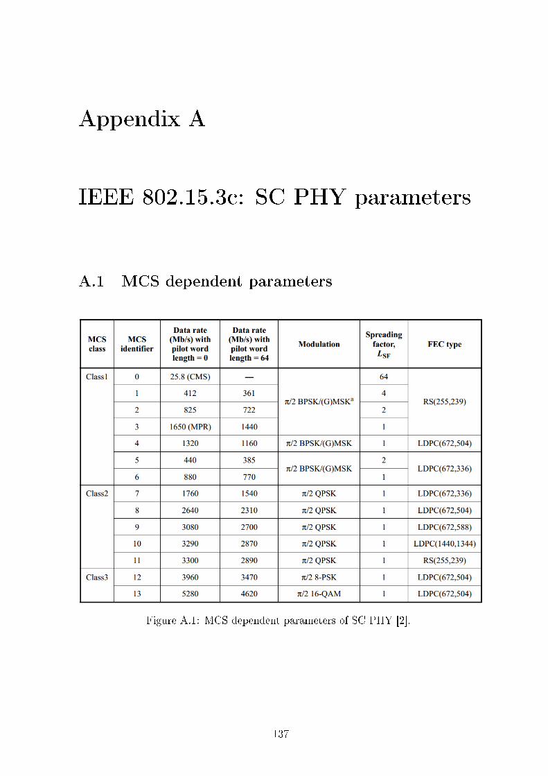
Appendix A
IEEE 802.15.3c: SC PHY parameters
A.1 MCS dependent parameters
Figure A.1: MCS dependent parameters of SC PHY [2].
137
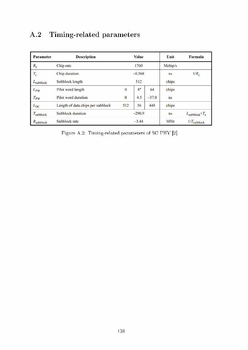
A.2 Timing-related parameters
Figure A.2: Timing-related parameters of SC PHY [2].
138
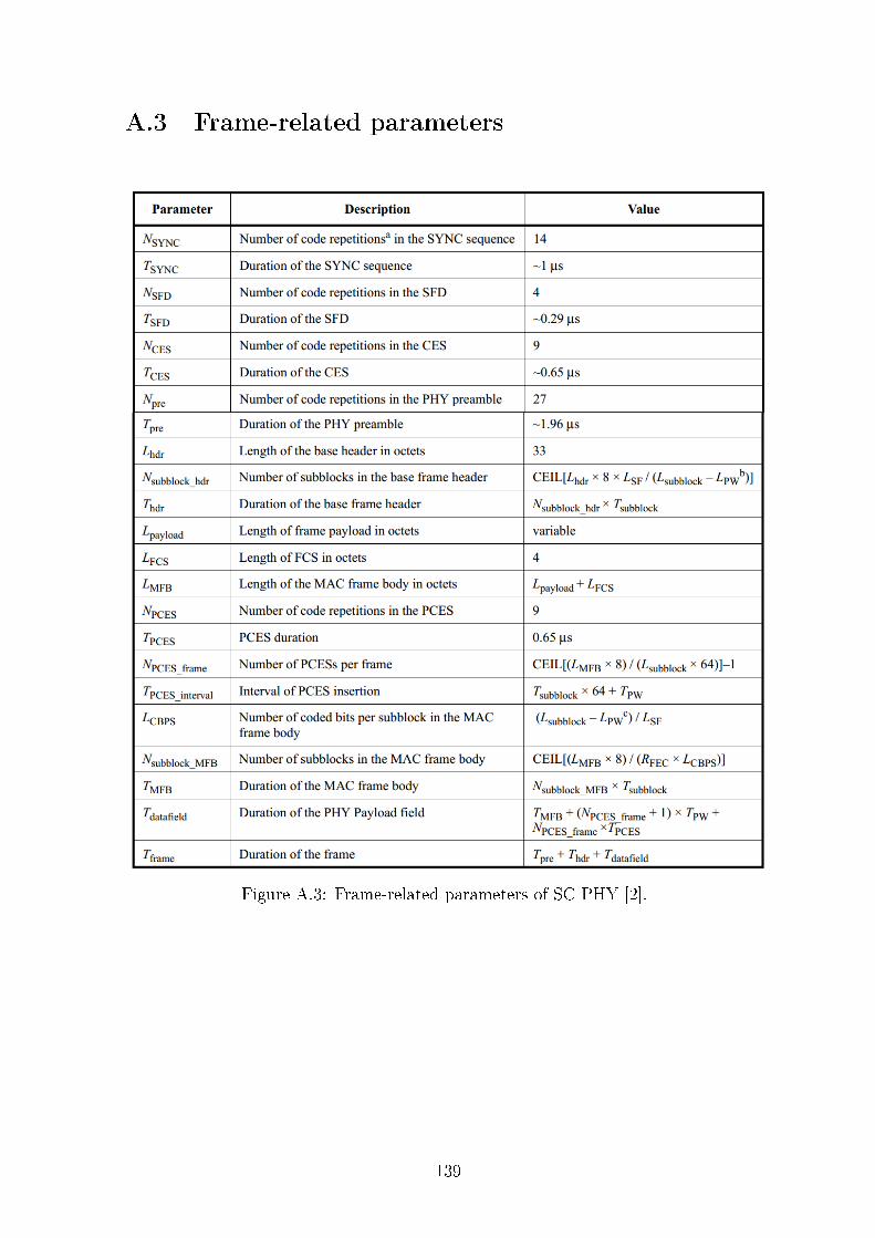
A.3 Frame-related parameters
Figure A.3: Frame-related parameters of SC PHY [2].
139
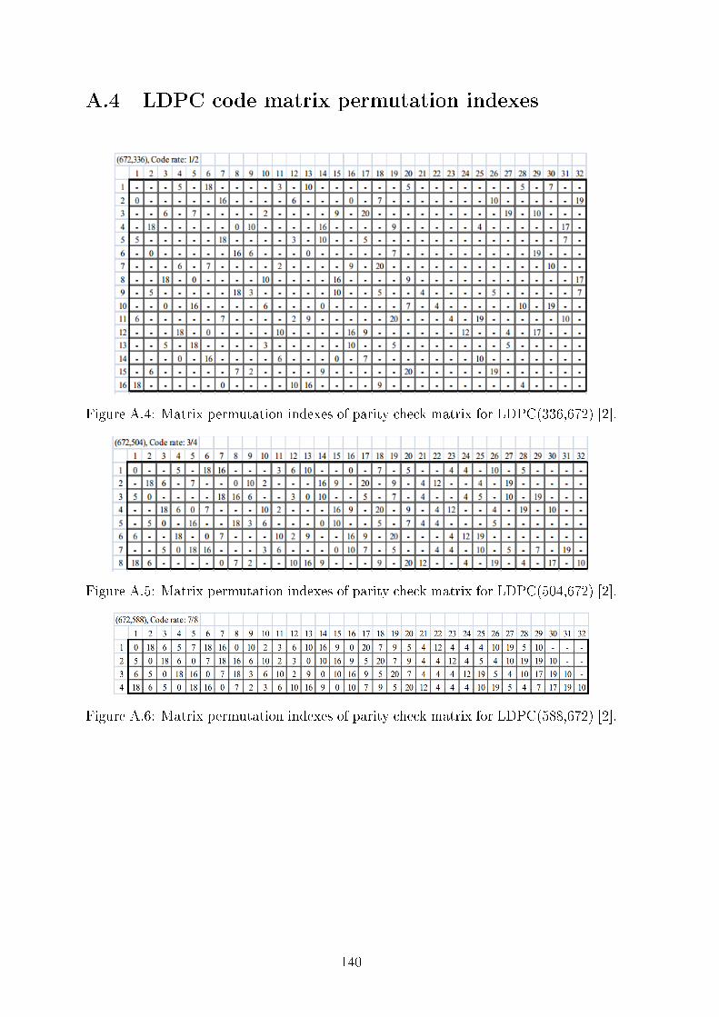
A.4 LDPC code matrix permutation indexes
Figure A.4: Matrix permutation indexes of parity check matrix for LDPC(336,672) [2].
Figure A.5: Matrix permutation indexes of parity check matrix for LDPC(504,672) [2].
Figure A.6: Matrix permutation indexes of parity check matrix for LDPC(588,672) [2].
140
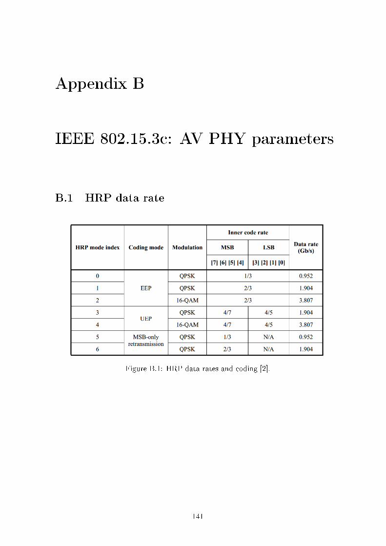
Appendix B
IEEE 802.15.3c: AV PHY parameters
B.1 HRP data rate
Figure B.1: HRP data rates and coding [2].
141
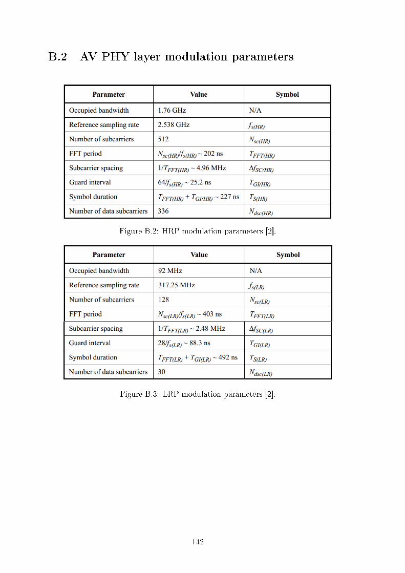
B.2 AV PHY layer modulation parameters
Figure B.2: HRP modulation parameters [2].
Figure B.3: LRP modulation parameters [2].
142
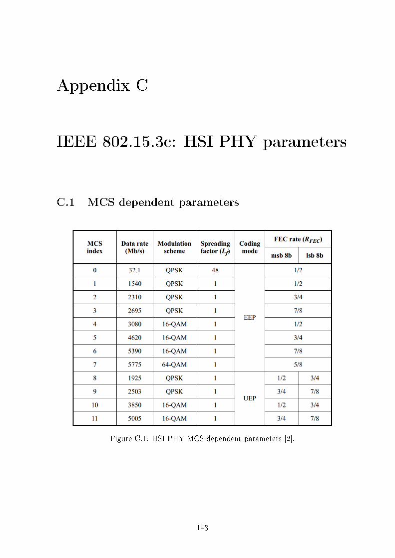
Appendix C
IEEE 802.15.3c: HSI PHY parameters
C.1 MCS dependent parameters
Figure C.1: HSI PHY MCS dependent parameters [2].
143
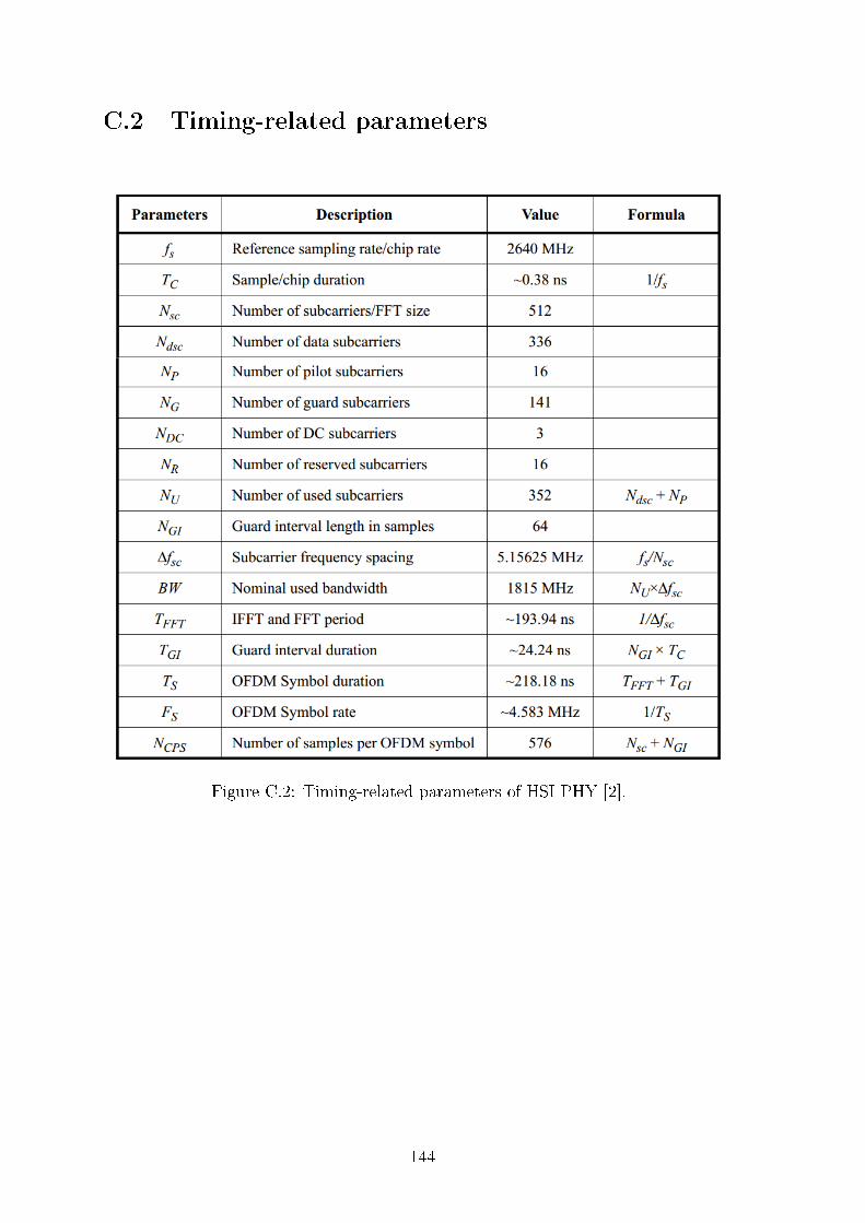
C.2 Timing-related parameters
Figure C.2: Timing-related parameters of HSI PHY [2].
144
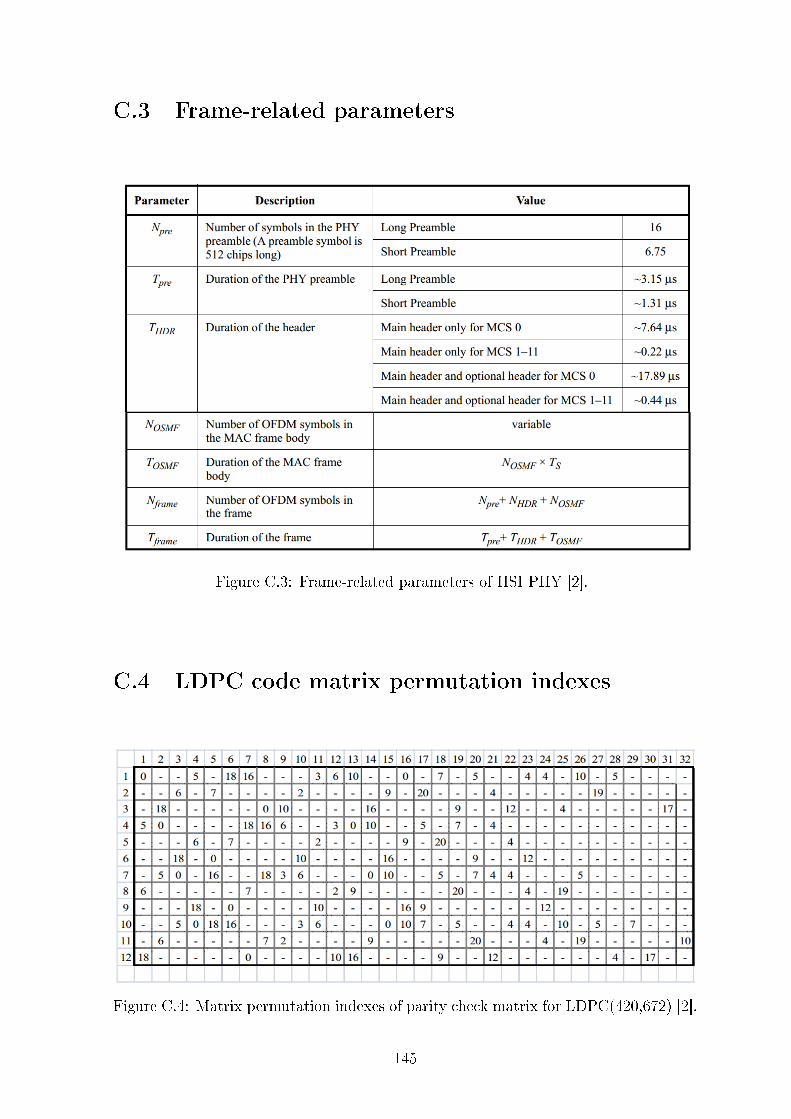
C.3 Frame-related parameters
Figure C.3: Frame-related parameters of HSI PHY [2].
C.4 LDPC code matrix permutation indexes
Figure C.4: Matrix permutation indexes of parity check matrix for LDPC(420,672) [2].
145
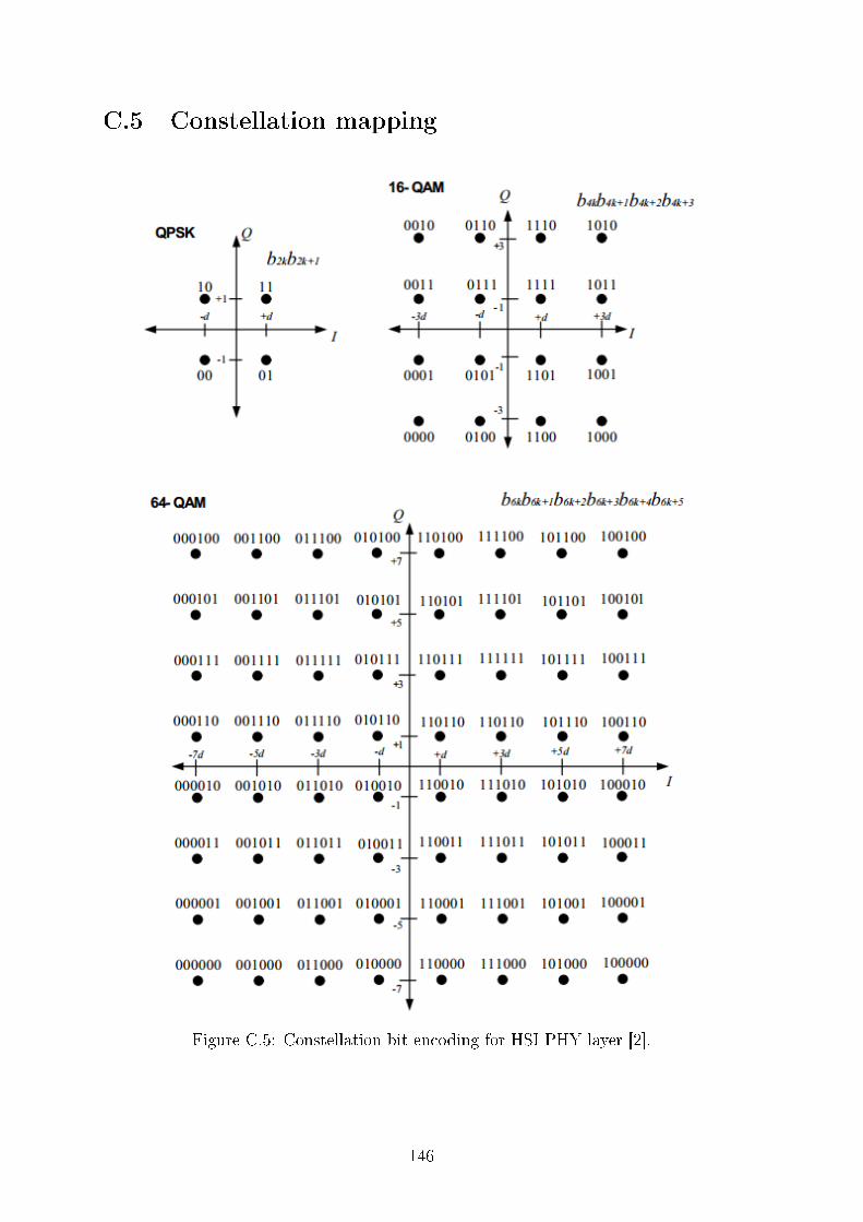
C.5 Constellation mapping
Figure C.5: Constellation bit encoding for HSI PHY layer [2].
146


![Inbound Selling Machine [How to Use Hubspot to Create Content that Sells]](https://img.pdfslide.tips/doc/110x75/55c35cd5bb61eb636f8b45b8/inbound-selling-machine-how-to-use-hubspot-to-create-content-that-sells.jpg)