Embed Size (px)
DESCRIPTION
CDF
Citation preview
Cumulative Distribution Functions Standard Normal Distribution
Cumulative Distribution Functions
Bernd Schroder
Bernd Schroder Louisiana Tech University, College of Engineering and Science
Cumulative Distribution Functions

Cumulative Distribution Functions Standard Normal Distribution
Introduction
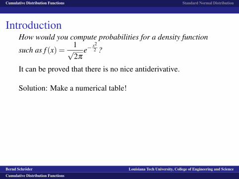
How would you compute probabilities for a density function
such as f (x) =1√2π
e−x22 ?
It can be proved that there is no nice antiderivative.
Solution: Make a numerical table!
Bernd Schroder Louisiana Tech University, College of Engineering and Science
Cumulative Distribution Functions
Cumulative Distribution Functions Standard Normal Distribution
IntroductionHow would you compute probabilities for a density function
such as f (x) =1√2π
e−x22 ?
It can be proved that there is no nice antiderivative.
Solution: Make a numerical table!
Bernd Schroder Louisiana Tech University, College of Engineering and Science
Cumulative Distribution Functions

Cumulative Distribution Functions Standard Normal Distribution
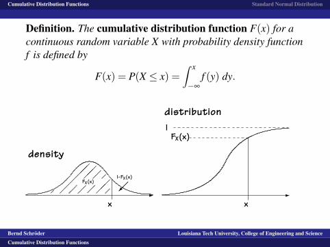
Definition.
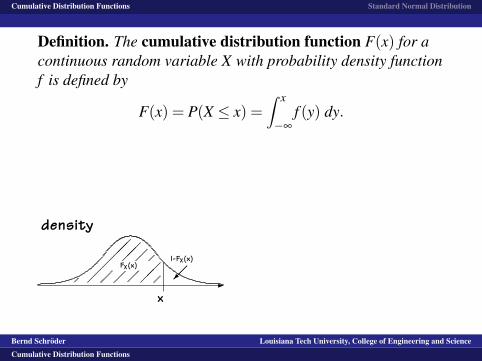
The cumulative distribution function F(x) for acontinuous random variable X with probability density functionf is defined by
F(x) = P(X ≤ x) =∫ x
−∞
f (y) dy.
density
-x
��
��
����FX(x)
��
l-FX(x)
distribution
-
l
x
FX(x)
?
6
l-FX(x)
Bernd Schroder Louisiana Tech University, College of Engineering and Science
Cumulative Distribution Functions
Cumulative Distribution Functions Standard Normal Distribution
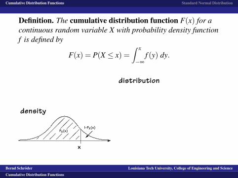
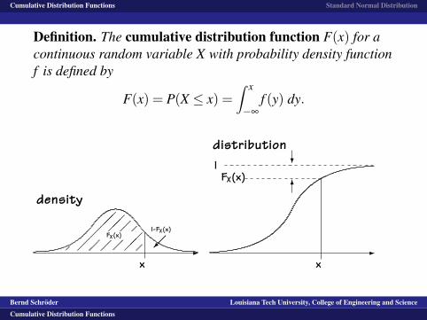
Definition. The cumulative distribution function F(x) for acontinuous random variable X with probability density functionf is defined by
F(x) = P(X ≤ x) =∫ x
−∞
f (y) dy.
density
-x
��
��
����FX(x)
��
l-FX(x)
distribution
-
l
x
FX(x)
?
6
l-FX(x)
Bernd Schroder Louisiana Tech University, College of Engineering and Science
Cumulative Distribution Functions
Cumulative Distribution Functions Standard Normal Distribution
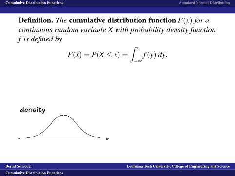
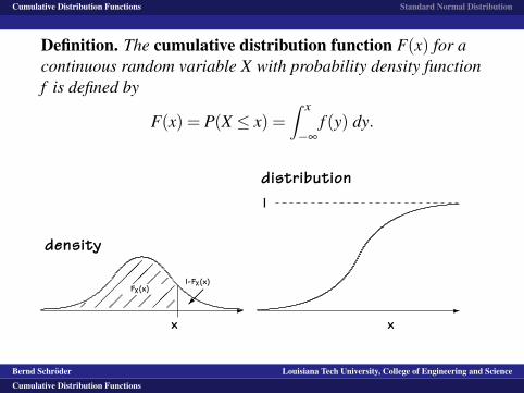
Definition. The cumulative distribution function F(x) for acontinuous random variable X with probability density functionf is defined by
F(x)
= P(X ≤ x) =∫ x
−∞
f (y) dy.
density
-x
��
��
����FX(x)
��
l-FX(x)
distribution
-
l
x
FX(x)
?
6
l-FX(x)
Bernd Schroder Louisiana Tech University, College of Engineering and Science
Cumulative Distribution Functions
Cumulative Distribution Functions Standard Normal Distribution
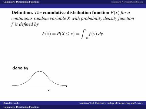
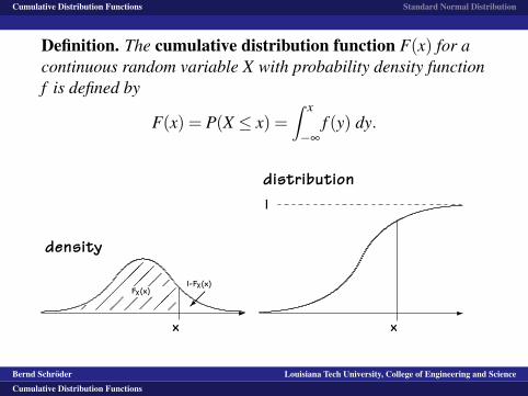
Definition. The cumulative distribution function F(x) for acontinuous random variable X with probability density functionf is defined by
F(x) = P(X ≤ x)
=∫ x
−∞
f (y) dy.
density
-x
��
��
����FX(x)
��
l-FX(x)
distribution
-
l
x
FX(x)
?
6
l-FX(x)
Bernd Schroder Louisiana Tech University, College of Engineering and Science
Cumulative Distribution Functions
Cumulative Distribution Functions Standard Normal Distribution
Definition. The cumulative distribution function F(x) for acontinuous random variable X with probability density functionf is defined by
F(x) = P(X ≤ x) =∫ x
−∞
f (y) dy.
density
-x
��
��
����FX(x)
��
l-FX(x)
distribution
-
l
x
FX(x)
?
6
l-FX(x)
Bernd Schroder Louisiana Tech University, College of Engineering and Science
Cumulative Distribution Functions
Cumulative Distribution Functions Standard Normal Distribution
Definition. The cumulative distribution function F(x) for acontinuous random variable X with probability density functionf is defined by
F(x) = P(X ≤ x) =∫ x
−∞
f (y) dy.
density
-
x
��
��
����FX(x)
��
l-FX(x)
distribution
-
l
x
FX(x)
?
6
l-FX(x)
Bernd Schroder Louisiana Tech University, College of Engineering and Science
Cumulative Distribution Functions
Cumulative Distribution Functions Standard Normal Distribution
Definition. The cumulative distribution function F(x) for acontinuous random variable X with probability density functionf is defined by
F(x) = P(X ≤ x) =∫ x
−∞
f (y) dy.
density
-x
��
��
����FX(x)
��
l-FX(x)
distribution
-
l
x
FX(x)
?
6
l-FX(x)
Bernd Schroder Louisiana Tech University, College of Engineering and Science
Cumulative Distribution Functions

Cumulative Distribution Functions Standard Normal Distribution
Definition. The cumulative distribution function F(x) for acontinuous random variable X with probability density functionf is defined by
F(x) = P(X ≤ x) =∫ x
−∞
f (y) dy.
density
-x
��
��
����
FX(x)
��
l-FX(x)
distribution
-
l
x
FX(x)
?
6
l-FX(x)
Bernd Schroder Louisiana Tech University, College of Engineering and Science
Cumulative Distribution Functions

Cumulative Distribution Functions Standard Normal Distribution
Definition. The cumulative distribution function F(x) for acontinuous random variable X with probability density functionf is defined by
F(x) = P(X ≤ x) =∫ x
−∞
f (y) dy.
density
-x
��
��
����FX(x)
��
l-FX(x)
distribution
-
l
x
FX(x)
?
6
l-FX(x)
Bernd Schroder Louisiana Tech University, College of Engineering and Science
Cumulative Distribution Functions

Cumulative Distribution Functions Standard Normal Distribution
Definition. The cumulative distribution function F(x) for acontinuous random variable X with probability density functionf is defined by
F(x) = P(X ≤ x) =∫ x
−∞
f (y) dy.
density
-x
��
��
����FX(x)
��
l-FX(x)
distribution
-
l
x
FX(x)
?
6
l-FX(x)
Bernd Schroder Louisiana Tech University, College of Engineering and Science
Cumulative Distribution Functions
Cumulative Distribution Functions Standard Normal Distribution
Cumulative Distribution Functions MeasureAggregate Area
Cumulative Distribution Function
Bernd Schroder Louisiana Tech University, College of Engineering and Science
Cumulative Distribution Functions
Cumulative Distribution Functions Standard Normal Distribution
Cumulative Distribution Functions MeasureAggregate Area
Cumulative Distribution FunctionBernd Schroder Louisiana Tech University, College of Engineering and Science
Cumulative Distribution Functions

Cumulative Distribution Functions Standard Normal Distribution
The Cumulative Distribution Function for theUniform Distribution
Cumulative Uniform Distribution Function
Bernd Schroder Louisiana Tech University, College of Engineering and Science
Cumulative Distribution Functions

Cumulative Distribution Functions Standard Normal Distribution
The Cumulative Distribution Function for theUniform Distribution
Cumulative Uniform Distribution Function
Bernd Schroder Louisiana Tech University, College of Engineering and Science
Cumulative Distribution Functions

Cumulative Distribution Functions Standard Normal Distribution
The Cumulative Distribution Function for theExponential Distribution
Cumulative Exponential Distribution Function
Bernd Schroder Louisiana Tech University, College of Engineering and Science
Cumulative Distribution Functions
Cumulative Distribution Functions Standard Normal Distribution
The Cumulative Distribution Function for theExponential Distribution
Cumulative Exponential Distribution Function
Bernd Schroder Louisiana Tech University, College of Engineering and Science
Cumulative Distribution Functions
Cumulative Distribution Functions Standard Normal Distribution
The Cumulative Distribution Function for theStandard Normal Distribution
Cumulative Normal Distribution Function
Bernd Schroder Louisiana Tech University, College of Engineering and Science
Cumulative Distribution Functions
Cumulative Distribution Functions Standard Normal Distribution
The Cumulative Distribution Function for theStandard Normal Distribution
Cumulative Normal Distribution FunctionBernd Schroder Louisiana Tech University, College of Engineering and Science
Cumulative Distribution Functions

Cumulative Distribution Functions Standard Normal Distribution
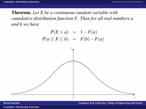
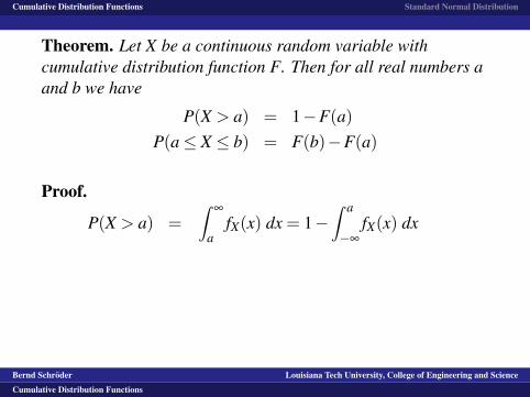
Theorem.
Let X be a continuous random variable withcumulative distribution function F. Then for all real numbers aand b we have
P(X > a) = 1−F(a)P(a≤ X ≤ b) = F(b)−F(a)
-z
6y
a
Bernd Schroder Louisiana Tech University, College of Engineering and Science
Cumulative Distribution Functions
Cumulative Distribution Functions Standard Normal Distribution
Theorem. Let X be a continuous random variable withcumulative distribution function F.
Then for all real numbers aand b we have
P(X > a) = 1−F(a)P(a≤ X ≤ b) = F(b)−F(a)
-z
6y
a
Bernd Schroder Louisiana Tech University, College of Engineering and Science
Cumulative Distribution Functions
Cumulative Distribution Functions Standard Normal Distribution
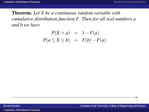
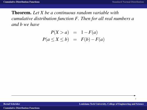
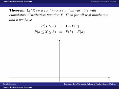
Theorem. Let X be a continuous random variable withcumulative distribution function F. Then for all real numbers aand b we have
P(X > a) = 1−F(a)P(a≤ X ≤ b) = F(b)−F(a)
-z
6y
a
Bernd Schroder Louisiana Tech University, College of Engineering and Science
Cumulative Distribution Functions
Cumulative Distribution Functions Standard Normal Distribution
Theorem. Let X be a continuous random variable withcumulative distribution function F. Then for all real numbers aand b we have
P(X > a)
= 1−F(a)P(a≤ X ≤ b) = F(b)−F(a)
-z
6y
a
Bernd Schroder Louisiana Tech University, College of Engineering and Science
Cumulative Distribution Functions

Cumulative Distribution Functions Standard Normal Distribution
Theorem. Let X be a continuous random variable withcumulative distribution function F. Then for all real numbers aand b we have
P(X > a) = 1−F(a)
P(a≤ X ≤ b) = F(b)−F(a)
-z
6y
a
Bernd Schroder Louisiana Tech University, College of Engineering and Science
Cumulative Distribution Functions
Cumulative Distribution Functions Standard Normal Distribution
Theorem. Let X be a continuous random variable withcumulative distribution function F. Then for all real numbers aand b we have
P(X > a) = 1−F(a)P(a≤ X ≤ b)
= F(b)−F(a)
-z
6y
a
Bernd Schroder Louisiana Tech University, College of Engineering and Science
Cumulative Distribution Functions
Cumulative Distribution Functions Standard Normal Distribution
Theorem. Let X be a continuous random variable withcumulative distribution function F. Then for all real numbers aand b we have
P(X > a) = 1−F(a)P(a≤ X ≤ b) = F(b)−F(a)
-z
6y
a
Bernd Schroder Louisiana Tech University, College of Engineering and Science
Cumulative Distribution Functions
Cumulative Distribution Functions Standard Normal Distribution
Theorem. Let X be a continuous random variable withcumulative distribution function F. Then for all real numbers aand b we have
P(X > a) = 1−F(a)P(a≤ X ≤ b) = F(b)−F(a)
-z
6y
a
Bernd Schroder Louisiana Tech University, College of Engineering and Science
Cumulative Distribution Functions
Cumulative Distribution Functions Standard Normal Distribution
Theorem. Let X be a continuous random variable withcumulative distribution function F. Then for all real numbers aand b we have
P(X > a) = 1−F(a)P(a≤ X ≤ b) = F(b)−F(a)
-z
6y
a
���
������
������
�������
��������
��������
��������
��������
���
Bernd Schroder Louisiana Tech University, College of Engineering and Science
Cumulative Distribution Functions

Cumulative Distribution Functions Standard Normal Distribution
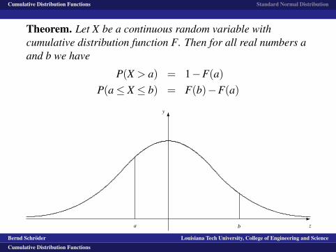
Theorem. Let X be a continuous random variable withcumulative distribution function F. Then for all real numbers aand b we have
P(X > a) = 1−F(a)P(a≤ X ≤ b) = F(b)−F(a)
-z
6y
a b
���
������
������
�������
������
�����
���
Bernd Schroder Louisiana Tech University, College of Engineering and Science
Cumulative Distribution Functions
Cumulative Distribution Functions Standard Normal Distribution
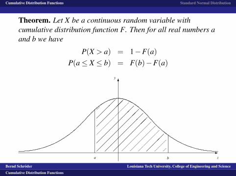
Theorem. Let X be a continuous random variable withcumulative distribution function F. Then for all real numbers aand b we have
P(X > a) = 1−F(a)P(a≤ X ≤ b) = F(b)−F(a)
-z
6y
a b
���
������
������
�������
������
�����
���
Bernd Schroder Louisiana Tech University, College of Engineering and Science
Cumulative Distribution Functions
Cumulative Distribution Functions Standard Normal Distribution
Theorem. Let X be a continuous random variable withcumulative distribution function F. Then for all real numbers aand b we have
P(X > a) = 1−F(a)P(a≤ X ≤ b) = F(b)−F(a)
-z
6y
a b
���
������
������
�������
������
�����
���
Bernd Schroder Louisiana Tech University, College of Engineering and Science
Cumulative Distribution Functions

Cumulative Distribution Functions Standard Normal Distribution
Theorem. Let X be a continuous random variable withcumulative distribution function F. Then for all real numbers aand b we have
P(X > a) = 1−F(a)P(a≤ X ≤ b) = F(b)−F(a)
-z
6y
a
b
���
������
������
�������
������
�����
���
Bernd Schroder Louisiana Tech University, College of Engineering and Science
Cumulative Distribution Functions
Cumulative Distribution Functions Standard Normal Distribution
Theorem. Let X be a continuous random variable withcumulative distribution function F. Then for all real numbers aand b we have
P(X > a) = 1−F(a)P(a≤ X ≤ b) = F(b)−F(a)
-z
6y
a b
���
������
������
�������
������
�����
���
Bernd Schroder Louisiana Tech University, College of Engineering and Science
Cumulative Distribution Functions

Cumulative Distribution Functions Standard Normal Distribution
Theorem. Let X be a continuous random variable withcumulative distribution function F. Then for all real numbers aand b we have
P(X > a) = 1−F(a)P(a≤ X ≤ b) = F(b)−F(a)
-z
6y
b
���
������
������
�������
��������
��������
��������
��������
���
Bernd Schroder Louisiana Tech University, College of Engineering and Science
Cumulative Distribution Functions
Cumulative Distribution Functions Standard Normal Distribution
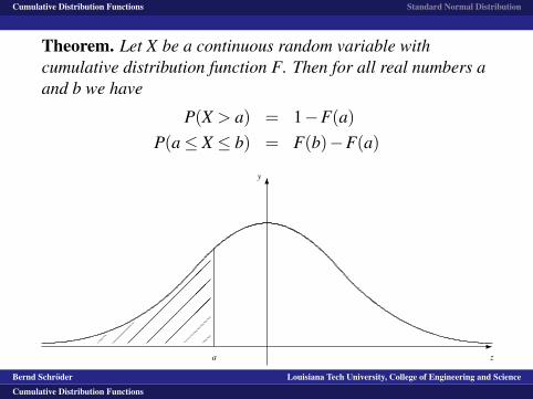
Theorem. Let X be a continuous random variable withcumulative distribution function F. Then for all real numbers aand b we have
P(X > a) = 1−F(a)P(a≤ X ≤ b) = F(b)−F(a)
-z
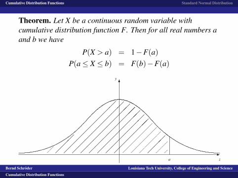
6y
a
����
�����
������
Bernd Schroder Louisiana Tech University, College of Engineering and Science
Cumulative Distribution Functions

Cumulative Distribution Functions Standard Normal Distribution
Theorem. Let X be a continuous random variable withcumulative distribution function F. Then for all real numbers aand b we have
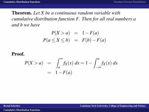
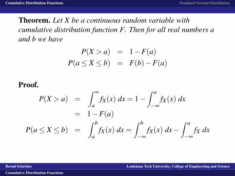
P(X > a) = 1−F(a)P(a≤ X ≤ b) = F(b)−F(a)
Proof.
P(X > a) =∫
∞
afX(x) dx = 1−
∫ a
−∞
fX(x) dx
= 1−F(a)
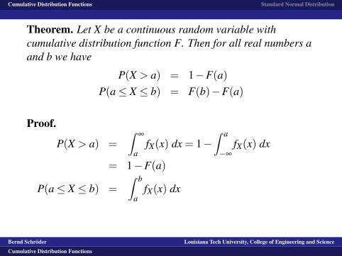
P(a≤ X ≤ b) =∫ b
afX(x) dx =
∫ b
−∞
fX(x) dx−∫ a
−∞
fX dx
= F(b)−F(a)
Bernd Schroder Louisiana Tech University, College of Engineering and Science
Cumulative Distribution Functions
Cumulative Distribution Functions Standard Normal Distribution
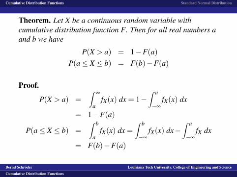
Theorem. Let X be a continuous random variable withcumulative distribution function F. Then for all real numbers aand b we have
P(X > a) = 1−F(a)P(a≤ X ≤ b) = F(b)−F(a)
Proof.
P(X > a) =∫
∞
afX(x) dx = 1−
∫ a
−∞
fX(x) dx
= 1−F(a)
P(a≤ X ≤ b) =∫ b
afX(x) dx =
∫ b
−∞
fX(x) dx−∫ a
−∞
fX dx
= F(b)−F(a)
Bernd Schroder Louisiana Tech University, College of Engineering and Science
Cumulative Distribution Functions
Cumulative Distribution Functions Standard Normal Distribution
Theorem. Let X be a continuous random variable withcumulative distribution function F. Then for all real numbers aand b we have
P(X > a) = 1−F(a)P(a≤ X ≤ b) = F(b)−F(a)
Proof.
P(X > a)
=∫
∞
afX(x) dx = 1−
∫ a
−∞
fX(x) dx
= 1−F(a)
P(a≤ X ≤ b) =∫ b
afX(x) dx =
∫ b
−∞
fX(x) dx−∫ a
−∞
fX dx
= F(b)−F(a)
Bernd Schroder Louisiana Tech University, College of Engineering and Science
Cumulative Distribution Functions
Cumulative Distribution Functions Standard Normal Distribution
Theorem. Let X be a continuous random variable withcumulative distribution function F. Then for all real numbers aand b we have
P(X > a) = 1−F(a)P(a≤ X ≤ b) = F(b)−F(a)
Proof.
P(X > a) =
∫∞
afX(x) dx = 1−
∫ a
−∞
fX(x) dx
= 1−F(a)
P(a≤ X ≤ b) =∫ b
afX(x) dx =
∫ b
−∞
fX(x) dx−∫ a
−∞
fX dx
= F(b)−F(a)
Bernd Schroder Louisiana Tech University, College of Engineering and Science
Cumulative Distribution Functions
Cumulative Distribution Functions Standard Normal Distribution
Theorem. Let X be a continuous random variable withcumulative distribution function F. Then for all real numbers aand b we have
P(X > a) = 1−F(a)P(a≤ X ≤ b) = F(b)−F(a)
Proof.
P(X > a) =∫
∞
afX(x) dx
= 1−∫ a
−∞
fX(x) dx
= 1−F(a)
P(a≤ X ≤ b) =∫ b
afX(x) dx =
∫ b
−∞
fX(x) dx−∫ a
−∞
fX dx
= F(b)−F(a)
Bernd Schroder Louisiana Tech University, College of Engineering and Science
Cumulative Distribution Functions
Cumulative Distribution Functions Standard Normal Distribution
Theorem. Let X be a continuous random variable withcumulative distribution function F. Then for all real numbers aand b we have
P(X > a) = 1−F(a)P(a≤ X ≤ b) = F(b)−F(a)
Proof.
P(X > a) =∫
∞
afX(x) dx = 1−
∫ a
−∞
fX(x) dx
= 1−F(a)
P(a≤ X ≤ b) =∫ b
afX(x) dx =
∫ b
−∞
fX(x) dx−∫ a
−∞
fX dx
= F(b)−F(a)
Bernd Schroder Louisiana Tech University, College of Engineering and Science
Cumulative Distribution Functions
Cumulative Distribution Functions Standard Normal Distribution
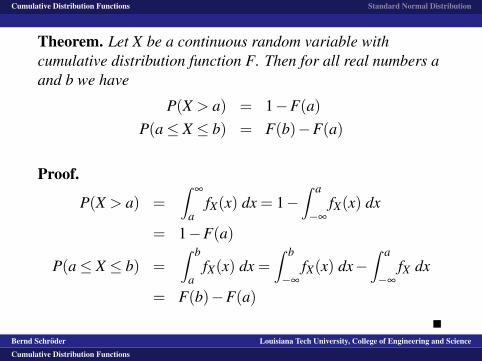
Theorem. Let X be a continuous random variable withcumulative distribution function F. Then for all real numbers aand b we have
P(X > a) = 1−F(a)P(a≤ X ≤ b) = F(b)−F(a)
Proof.
P(X > a) =∫
∞
afX(x) dx = 1−
∫ a
−∞
fX(x) dx
= 1−F(a)
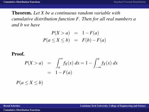
P(a≤ X ≤ b)
=∫ b
afX(x) dx =
∫ b
−∞
fX(x) dx−∫ a
−∞
fX dx
= F(b)−F(a)
Bernd Schroder Louisiana Tech University, College of Engineering and Science
Cumulative Distribution Functions

Cumulative Distribution Functions Standard Normal Distribution
Theorem. Let X be a continuous random variable withcumulative distribution function F. Then for all real numbers aand b we have
P(X > a) = 1−F(a)P(a≤ X ≤ b) = F(b)−F(a)
Proof.
P(X > a) =∫
∞
afX(x) dx = 1−
∫ a
−∞
fX(x) dx
= 1−F(a)
P(a≤ X ≤ b) =
∫ b
afX(x) dx =
∫ b
−∞
fX(x) dx−∫ a
−∞
fX dx
= F(b)−F(a)
Bernd Schroder Louisiana Tech University, College of Engineering and Science
Cumulative Distribution Functions
Cumulative Distribution Functions Standard Normal Distribution
Theorem. Let X be a continuous random variable withcumulative distribution function F. Then for all real numbers aand b we have
P(X > a) = 1−F(a)P(a≤ X ≤ b) = F(b)−F(a)
Proof.
P(X > a) =∫
∞
afX(x) dx = 1−
∫ a
−∞
fX(x) dx
= 1−F(a)
P(a≤ X ≤ b) =∫ b
afX(x) dx
=∫ b
−∞
fX(x) dx−∫ a
−∞
fX dx
= F(b)−F(a)
Bernd Schroder Louisiana Tech University, College of Engineering and Science
Cumulative Distribution Functions
Cumulative Distribution Functions Standard Normal Distribution
Theorem. Let X be a continuous random variable withcumulative distribution function F. Then for all real numbers aand b we have
P(X > a) = 1−F(a)P(a≤ X ≤ b) = F(b)−F(a)
Proof.
P(X > a) =∫
∞
afX(x) dx = 1−
∫ a
−∞
fX(x) dx
= 1−F(a)
P(a≤ X ≤ b) =∫ b
afX(x) dx =
∫ b
−∞
fX(x) dx−∫ a
−∞
fX dx
= F(b)−F(a)
Bernd Schroder Louisiana Tech University, College of Engineering and Science
Cumulative Distribution Functions
Cumulative Distribution Functions Standard Normal Distribution
Theorem. Let X be a continuous random variable withcumulative distribution function F. Then for all real numbers aand b we have
P(X > a) = 1−F(a)P(a≤ X ≤ b) = F(b)−F(a)
Proof.
P(X > a) =∫
∞
afX(x) dx = 1−
∫ a
−∞
fX(x) dx
= 1−F(a)
P(a≤ X ≤ b) =∫ b
afX(x) dx =
∫ b
−∞
fX(x) dx−∫ a
−∞
fX dx
= F(b)−F(a)
Bernd Schroder Louisiana Tech University, College of Engineering and Science
Cumulative Distribution Functions

Cumulative Distribution Functions Standard Normal Distribution
Theorem.
Let X be a continuous random variable withcumulative distribution function F and probability densityfunction f . Then
f (x) =ddx
F(x).
Proof.ddx
F(x) =ddx
∫ x
−∞
f (t) dt
=ddx
[∫ 0
−∞
f (t) dt+∫ x
0f (t) dt
]= 0+ f (x) = f (x)
Bernd Schroder Louisiana Tech University, College of Engineering and Science
Cumulative Distribution Functions
Cumulative Distribution Functions Standard Normal Distribution
Theorem. Let X be a continuous random variable withcumulative distribution function F and probability densityfunction f .
Then
f (x) =ddx
F(x).
Proof.ddx
F(x) =ddx
∫ x
−∞
f (t) dt
=ddx
[∫ 0
−∞
f (t) dt+∫ x
0f (t) dt
]= 0+ f (x) = f (x)
Bernd Schroder Louisiana Tech University, College of Engineering and Science
Cumulative Distribution Functions
Cumulative Distribution Functions Standard Normal Distribution
Theorem. Let X be a continuous random variable withcumulative distribution function F and probability densityfunction f . Then
f (x) =ddx
F(x).
Proof.
ddx
F(x) =ddx
∫ x
−∞
f (t) dt
=ddx
[∫ 0
−∞
f (t) dt+∫ x
0f (t) dt
]= 0+ f (x) = f (x)
Bernd Schroder Louisiana Tech University, College of Engineering and Science
Cumulative Distribution Functions
Cumulative Distribution Functions Standard Normal Distribution
Theorem. Let X be a continuous random variable withcumulative distribution function F and probability densityfunction f . Then
f (x) =ddx
F(x).
Proof.ddx
F(x)
=ddx
∫ x
−∞
f (t) dt
=ddx
[∫ 0
−∞
f (t) dt+∫ x
0f (t) dt
]= 0+ f (x) = f (x)
Bernd Schroder Louisiana Tech University, College of Engineering and Science
Cumulative Distribution Functions
Cumulative Distribution Functions Standard Normal Distribution
Theorem. Let X be a continuous random variable withcumulative distribution function F and probability densityfunction f . Then
f (x) =ddx
F(x).
Proof.ddx
F(x) =ddx
∫ x
−∞
f (t) dt
=ddx
[∫ 0
−∞
f (t) dt+∫ x
0f (t) dt
]= 0+ f (x) = f (x)
Bernd Schroder Louisiana Tech University, College of Engineering and Science
Cumulative Distribution Functions
Cumulative Distribution Functions Standard Normal Distribution
Theorem. Let X be a continuous random variable withcumulative distribution function F and probability densityfunction f . Then
f (x) =ddx
F(x).
Proof.ddx
F(x) =ddx
∫ x
−∞
f (t) dt
=ddx
[∫ 0
−∞
f (t) dt+∫ x
0f (t) dt
]
= 0+ f (x) = f (x)
Bernd Schroder Louisiana Tech University, College of Engineering and Science
Cumulative Distribution Functions
Cumulative Distribution Functions Standard Normal Distribution
Theorem. Let X be a continuous random variable withcumulative distribution function F and probability densityfunction f . Then
f (x) =ddx
F(x).
Proof.ddx
F(x) =ddx
∫ x
−∞
f (t) dt
=ddx
[∫ 0
−∞
f (t) dt+∫ x
0f (t) dt
]= 0+ f (x)
= f (x)
Bernd Schroder Louisiana Tech University, College of Engineering and Science
Cumulative Distribution Functions
Cumulative Distribution Functions Standard Normal Distribution
Theorem. Let X be a continuous random variable withcumulative distribution function F and probability densityfunction f . Then
f (x) =ddx
F(x).
Proof.ddx
F(x) =ddx
∫ x
−∞
f (t) dt
=ddx
[∫ 0
−∞
f (t) dt+∫ x
0f (t) dt
]= 0+ f (x) = f (x)
Bernd Schroder Louisiana Tech University, College of Engineering and Science
Cumulative Distribution Functions
Cumulative Distribution Functions Standard Normal Distribution
Theorem. Let X be a continuous random variable withcumulative distribution function F and probability densityfunction f . Then
f (x) =ddx
F(x).
Proof.ddx
F(x) =ddx
∫ x
−∞
f (t) dt
=ddx
[∫ 0
−∞
f (t) dt+∫ x
0f (t) dt
]= 0+ f (x) = f (x)
Bernd Schroder Louisiana Tech University, College of Engineering and Science
Cumulative Distribution Functions

Cumulative Distribution Functions Standard Normal Distribution
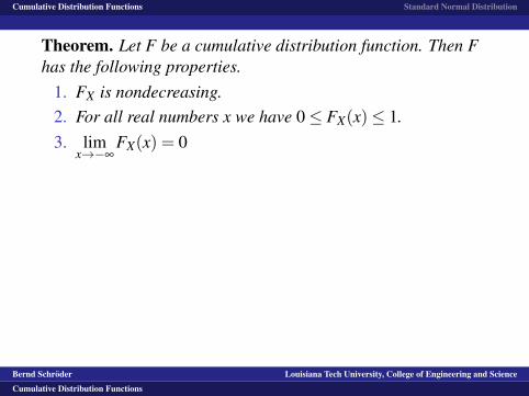
Theorem.
Let F be a cumulative distribution function. Then Fhas the following properties.
1. FX is nondecreasing.2. For all real numbers x we have 0≤ FX(x)≤ 1.3. lim
x→−∞FX(x) = 0 and lim
x→∞FX(x) = 1.
Proof. Part 1: If a < b, thenFX(a) = P(X < a)≤ P(X < a)+P(a≤ X < b) = P(X < b) = FX(b).Part 2: Follows from the fact that probabilities are nonnegativeand never exceed 1.Part 3:lim
x→−∞FX(x) = P(X is not a real number) = 0
limx→∞
FX(x) = P(−∞ < X < ∞) = 1
Bernd Schroder Louisiana Tech University, College of Engineering and Science
Cumulative Distribution Functions
Cumulative Distribution Functions Standard Normal Distribution
Theorem. Let F be a cumulative distribution function.
Then Fhas the following properties.
1. FX is nondecreasing.2. For all real numbers x we have 0≤ FX(x)≤ 1.3. lim
x→−∞FX(x) = 0 and lim
x→∞FX(x) = 1.
Proof. Part 1: If a < b, thenFX(a) = P(X < a)≤ P(X < a)+P(a≤ X < b) = P(X < b) = FX(b).Part 2: Follows from the fact that probabilities are nonnegativeand never exceed 1.Part 3:lim
x→−∞FX(x) = P(X is not a real number) = 0
limx→∞
FX(x) = P(−∞ < X < ∞) = 1
Bernd Schroder Louisiana Tech University, College of Engineering and Science
Cumulative Distribution Functions
Cumulative Distribution Functions Standard Normal Distribution
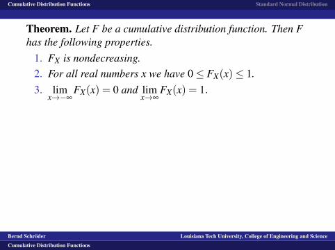
Theorem. Let F be a cumulative distribution function. Then Fhas the following properties.
1. FX is nondecreasing.2. For all real numbers x we have 0≤ FX(x)≤ 1.3. lim
x→−∞FX(x) = 0 and lim
x→∞FX(x) = 1.
Proof. Part 1: If a < b, thenFX(a) = P(X < a)≤ P(X < a)+P(a≤ X < b) = P(X < b) = FX(b).Part 2: Follows from the fact that probabilities are nonnegativeand never exceed 1.Part 3:lim
x→−∞FX(x) = P(X is not a real number) = 0
limx→∞
FX(x) = P(−∞ < X < ∞) = 1
Bernd Schroder Louisiana Tech University, College of Engineering and Science
Cumulative Distribution Functions
Cumulative Distribution Functions Standard Normal Distribution
Theorem. Let F be a cumulative distribution function. Then Fhas the following properties.
1. FX is nondecreasing.
2. For all real numbers x we have 0≤ FX(x)≤ 1.3. lim
x→−∞FX(x) = 0 and lim
x→∞FX(x) = 1.
Proof. Part 1: If a < b, thenFX(a) = P(X < a)≤ P(X < a)+P(a≤ X < b) = P(X < b) = FX(b).Part 2: Follows from the fact that probabilities are nonnegativeand never exceed 1.Part 3:lim
x→−∞FX(x) = P(X is not a real number) = 0
limx→∞
FX(x) = P(−∞ < X < ∞) = 1
Bernd Schroder Louisiana Tech University, College of Engineering and Science
Cumulative Distribution Functions
Cumulative Distribution Functions Standard Normal Distribution
Theorem. Let F be a cumulative distribution function. Then Fhas the following properties.
1. FX is nondecreasing.2. For all real numbers x we have 0≤ FX(x)≤ 1.
3. limx→−∞
FX(x) = 0 and limx→∞
FX(x) = 1.
Proof. Part 1: If a < b, thenFX(a) = P(X < a)≤ P(X < a)+P(a≤ X < b) = P(X < b) = FX(b).Part 2: Follows from the fact that probabilities are nonnegativeand never exceed 1.Part 3:lim
x→−∞FX(x) = P(X is not a real number) = 0
limx→∞
FX(x) = P(−∞ < X < ∞) = 1
Bernd Schroder Louisiana Tech University, College of Engineering and Science
Cumulative Distribution Functions
Cumulative Distribution Functions Standard Normal Distribution
Theorem. Let F be a cumulative distribution function. Then Fhas the following properties.
1. FX is nondecreasing.2. For all real numbers x we have 0≤ FX(x)≤ 1.3. lim
x→−∞FX(x) = 0
and limx→∞
FX(x) = 1.
Proof. Part 1: If a < b, thenFX(a) = P(X < a)≤ P(X < a)+P(a≤ X < b) = P(X < b) = FX(b).Part 2: Follows from the fact that probabilities are nonnegativeand never exceed 1.Part 3:lim
x→−∞FX(x) = P(X is not a real number) = 0
limx→∞
FX(x) = P(−∞ < X < ∞) = 1
Bernd Schroder Louisiana Tech University, College of Engineering and Science
Cumulative Distribution Functions
Cumulative Distribution Functions Standard Normal Distribution
Theorem. Let F be a cumulative distribution function. Then Fhas the following properties.
1. FX is nondecreasing.2. For all real numbers x we have 0≤ FX(x)≤ 1.3. lim
x→−∞FX(x) = 0 and lim
x→∞FX(x) = 1.
Proof. Part 1: If a < b, thenFX(a) = P(X < a)≤ P(X < a)+P(a≤ X < b) = P(X < b) = FX(b).Part 2: Follows from the fact that probabilities are nonnegativeand never exceed 1.Part 3:lim
x→−∞FX(x) = P(X is not a real number) = 0
limx→∞
FX(x) = P(−∞ < X < ∞) = 1
Bernd Schroder Louisiana Tech University, College of Engineering and Science
Cumulative Distribution Functions
Cumulative Distribution Functions Standard Normal Distribution
Theorem. Let F be a cumulative distribution function. Then Fhas the following properties.
1. FX is nondecreasing.2. For all real numbers x we have 0≤ FX(x)≤ 1.3. lim
x→−∞FX(x) = 0 and lim
x→∞FX(x) = 1.
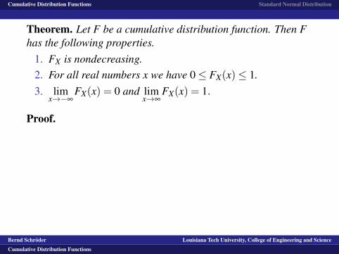
Proof.
Part 1: If a < b, thenFX(a) = P(X < a)≤ P(X < a)+P(a≤ X < b) = P(X < b) = FX(b).Part 2: Follows from the fact that probabilities are nonnegativeand never exceed 1.Part 3:lim
x→−∞FX(x) = P(X is not a real number) = 0
limx→∞
FX(x) = P(−∞ < X < ∞) = 1
Bernd Schroder Louisiana Tech University, College of Engineering and Science
Cumulative Distribution Functions
Cumulative Distribution Functions Standard Normal Distribution
Theorem. Let F be a cumulative distribution function. Then Fhas the following properties.
1. FX is nondecreasing.2. For all real numbers x we have 0≤ FX(x)≤ 1.3. lim
x→−∞FX(x) = 0 and lim
x→∞FX(x) = 1.
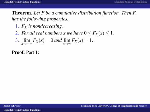
Proof. Part 1:
If a < b, thenFX(a) = P(X < a)≤ P(X < a)+P(a≤ X < b) = P(X < b) = FX(b).Part 2: Follows from the fact that probabilities are nonnegativeand never exceed 1.Part 3:lim
x→−∞FX(x) = P(X is not a real number) = 0
limx→∞
FX(x) = P(−∞ < X < ∞) = 1
Bernd Schroder Louisiana Tech University, College of Engineering and Science
Cumulative Distribution Functions
Cumulative Distribution Functions Standard Normal Distribution
Theorem. Let F be a cumulative distribution function. Then Fhas the following properties.
1. FX is nondecreasing.2. For all real numbers x we have 0≤ FX(x)≤ 1.3. lim
x→−∞FX(x) = 0 and lim
x→∞FX(x) = 1.
Proof. Part 1: If a < b, then
FX(a) = P(X < a)≤ P(X < a)+P(a≤ X < b) = P(X < b) = FX(b).Part 2: Follows from the fact that probabilities are nonnegativeand never exceed 1.Part 3:lim
x→−∞FX(x) = P(X is not a real number) = 0
limx→∞
FX(x) = P(−∞ < X < ∞) = 1
Bernd Schroder Louisiana Tech University, College of Engineering and Science
Cumulative Distribution Functions
Cumulative Distribution Functions Standard Normal Distribution
Theorem. Let F be a cumulative distribution function. Then Fhas the following properties.
1. FX is nondecreasing.2. For all real numbers x we have 0≤ FX(x)≤ 1.3. lim
x→−∞FX(x) = 0 and lim
x→∞FX(x) = 1.
Proof. Part 1: If a < b, thenFX(a)
= P(X < a)≤ P(X < a)+P(a≤ X < b) = P(X < b) = FX(b).Part 2: Follows from the fact that probabilities are nonnegativeand never exceed 1.Part 3:lim
x→−∞FX(x) = P(X is not a real number) = 0
limx→∞
FX(x) = P(−∞ < X < ∞) = 1
Bernd Schroder Louisiana Tech University, College of Engineering and Science
Cumulative Distribution Functions

Cumulative Distribution Functions Standard Normal Distribution
Theorem. Let F be a cumulative distribution function. Then Fhas the following properties.
1. FX is nondecreasing.2. For all real numbers x we have 0≤ FX(x)≤ 1.3. lim
x→−∞FX(x) = 0 and lim
x→∞FX(x) = 1.
Proof. Part 1: If a < b, thenFX(a) = P(X < a)
≤ P(X < a)+P(a≤ X < b) = P(X < b) = FX(b).Part 2: Follows from the fact that probabilities are nonnegativeand never exceed 1.Part 3:lim
x→−∞FX(x) = P(X is not a real number) = 0
limx→∞
FX(x) = P(−∞ < X < ∞) = 1
Bernd Schroder Louisiana Tech University, College of Engineering and Science
Cumulative Distribution Functions

Cumulative Distribution Functions Standard Normal Distribution
Theorem. Let F be a cumulative distribution function. Then Fhas the following properties.
1. FX is nondecreasing.2. For all real numbers x we have 0≤ FX(x)≤ 1.3. lim
x→−∞FX(x) = 0 and lim
x→∞FX(x) = 1.
Proof. Part 1: If a < b, thenFX(a) = P(X < a)≤ P(X < a)+P(a≤ X < b)
= P(X < b) = FX(b).Part 2: Follows from the fact that probabilities are nonnegativeand never exceed 1.Part 3:lim
x→−∞FX(x) = P(X is not a real number) = 0
limx→∞
FX(x) = P(−∞ < X < ∞) = 1
Bernd Schroder Louisiana Tech University, College of Engineering and Science
Cumulative Distribution Functions
Cumulative Distribution Functions Standard Normal Distribution
Theorem. Let F be a cumulative distribution function. Then Fhas the following properties.
1. FX is nondecreasing.2. For all real numbers x we have 0≤ FX(x)≤ 1.3. lim
x→−∞FX(x) = 0 and lim
x→∞FX(x) = 1.
Proof. Part 1: If a < b, thenFX(a) = P(X < a)≤ P(X < a)+P(a≤ X < b) = P(X < b)
= FX(b).Part 2: Follows from the fact that probabilities are nonnegativeand never exceed 1.Part 3:lim
x→−∞FX(x) = P(X is not a real number) = 0
limx→∞
FX(x) = P(−∞ < X < ∞) = 1
Bernd Schroder Louisiana Tech University, College of Engineering and Science
Cumulative Distribution Functions
Cumulative Distribution Functions Standard Normal Distribution
Theorem. Let F be a cumulative distribution function. Then Fhas the following properties.
1. FX is nondecreasing.2. For all real numbers x we have 0≤ FX(x)≤ 1.3. lim
x→−∞FX(x) = 0 and lim
x→∞FX(x) = 1.
Proof. Part 1: If a < b, thenFX(a) = P(X < a)≤ P(X < a)+P(a≤ X < b) = P(X < b) = FX(b).
Part 2: Follows from the fact that probabilities are nonnegativeand never exceed 1.Part 3:lim
x→−∞FX(x) = P(X is not a real number) = 0
limx→∞
FX(x) = P(−∞ < X < ∞) = 1
Bernd Schroder Louisiana Tech University, College of Engineering and Science
Cumulative Distribution Functions

Cumulative Distribution Functions Standard Normal Distribution
Theorem. Let F be a cumulative distribution function. Then Fhas the following properties.
1. FX is nondecreasing.2. For all real numbers x we have 0≤ FX(x)≤ 1.3. lim
x→−∞FX(x) = 0 and lim
x→∞FX(x) = 1.
Proof. Part 1: If a < b, thenFX(a) = P(X < a)≤ P(X < a)+P(a≤ X < b) = P(X < b) = FX(b).Part 2:
Follows from the fact that probabilities are nonnegativeand never exceed 1.Part 3:lim
x→−∞FX(x) = P(X is not a real number) = 0
limx→∞
FX(x) = P(−∞ < X < ∞) = 1
Bernd Schroder Louisiana Tech University, College of Engineering and Science
Cumulative Distribution Functions
Cumulative Distribution Functions Standard Normal Distribution
Theorem. Let F be a cumulative distribution function. Then Fhas the following properties.
1. FX is nondecreasing.2. For all real numbers x we have 0≤ FX(x)≤ 1.3. lim
x→−∞FX(x) = 0 and lim
x→∞FX(x) = 1.
Proof. Part 1: If a < b, thenFX(a) = P(X < a)≤ P(X < a)+P(a≤ X < b) = P(X < b) = FX(b).Part 2: Follows from the fact that probabilities are nonnegativeand never exceed 1.
Part 3:lim
x→−∞FX(x) = P(X is not a real number) = 0
limx→∞
FX(x) = P(−∞ < X < ∞) = 1
Bernd Schroder Louisiana Tech University, College of Engineering and Science
Cumulative Distribution Functions

Cumulative Distribution Functions Standard Normal Distribution
Theorem. Let F be a cumulative distribution function. Then Fhas the following properties.
1. FX is nondecreasing.2. For all real numbers x we have 0≤ FX(x)≤ 1.3. lim
x→−∞FX(x) = 0 and lim
x→∞FX(x) = 1.
Proof. Part 1: If a < b, thenFX(a) = P(X < a)≤ P(X < a)+P(a≤ X < b) = P(X < b) = FX(b).Part 2: Follows from the fact that probabilities are nonnegativeand never exceed 1.Part 3:
limx→−∞
FX(x) = P(X is not a real number) = 0
limx→∞
FX(x) = P(−∞ < X < ∞) = 1
Bernd Schroder Louisiana Tech University, College of Engineering and Science
Cumulative Distribution Functions
Cumulative Distribution Functions Standard Normal Distribution
Theorem. Let F be a cumulative distribution function. Then Fhas the following properties.
1. FX is nondecreasing.2. For all real numbers x we have 0≤ FX(x)≤ 1.3. lim
x→−∞FX(x) = 0 and lim
x→∞FX(x) = 1.
Proof. Part 1: If a < b, thenFX(a) = P(X < a)≤ P(X < a)+P(a≤ X < b) = P(X < b) = FX(b).Part 2: Follows from the fact that probabilities are nonnegativeand never exceed 1.Part 3:lim
x→−∞FX(x)
= P(X is not a real number) = 0
limx→∞
FX(x) = P(−∞ < X < ∞) = 1
Bernd Schroder Louisiana Tech University, College of Engineering and Science
Cumulative Distribution Functions
Cumulative Distribution Functions Standard Normal Distribution
Theorem. Let F be a cumulative distribution function. Then Fhas the following properties.
1. FX is nondecreasing.2. For all real numbers x we have 0≤ FX(x)≤ 1.3. lim
x→−∞FX(x) = 0 and lim
x→∞FX(x) = 1.
Proof. Part 1: If a < b, thenFX(a) = P(X < a)≤ P(X < a)+P(a≤ X < b) = P(X < b) = FX(b).Part 2: Follows from the fact that probabilities are nonnegativeand never exceed 1.Part 3:lim
x→−∞FX(x) = P(X is not a real number)
= 0
limx→∞
FX(x) = P(−∞ < X < ∞) = 1
Bernd Schroder Louisiana Tech University, College of Engineering and Science
Cumulative Distribution Functions
Cumulative Distribution Functions Standard Normal Distribution
Theorem. Let F be a cumulative distribution function. Then Fhas the following properties.
1. FX is nondecreasing.2. For all real numbers x we have 0≤ FX(x)≤ 1.3. lim
x→−∞FX(x) = 0 and lim
x→∞FX(x) = 1.
Proof. Part 1: If a < b, thenFX(a) = P(X < a)≤ P(X < a)+P(a≤ X < b) = P(X < b) = FX(b).Part 2: Follows from the fact that probabilities are nonnegativeand never exceed 1.Part 3:lim
x→−∞FX(x) = P(X is not a real number) = 0
limx→∞
FX(x) = P(−∞ < X < ∞) = 1
Bernd Schroder Louisiana Tech University, College of Engineering and Science
Cumulative Distribution Functions
Cumulative Distribution Functions Standard Normal Distribution
Theorem. Let F be a cumulative distribution function. Then Fhas the following properties.
1. FX is nondecreasing.2. For all real numbers x we have 0≤ FX(x)≤ 1.3. lim
x→−∞FX(x) = 0 and lim
x→∞FX(x) = 1.
Proof. Part 1: If a < b, thenFX(a) = P(X < a)≤ P(X < a)+P(a≤ X < b) = P(X < b) = FX(b).Part 2: Follows from the fact that probabilities are nonnegativeand never exceed 1.Part 3:lim
x→−∞FX(x) = P(X is not a real number) = 0
limx→∞
FX(x)
= P(−∞ < X < ∞) = 1
Bernd Schroder Louisiana Tech University, College of Engineering and Science
Cumulative Distribution Functions
Cumulative Distribution Functions Standard Normal Distribution
Theorem. Let F be a cumulative distribution function. Then Fhas the following properties.
1. FX is nondecreasing.2. For all real numbers x we have 0≤ FX(x)≤ 1.3. lim
x→−∞FX(x) = 0 and lim
x→∞FX(x) = 1.
Proof. Part 1: If a < b, thenFX(a) = P(X < a)≤ P(X < a)+P(a≤ X < b) = P(X < b) = FX(b).Part 2: Follows from the fact that probabilities are nonnegativeand never exceed 1.Part 3:lim
x→−∞FX(x) = P(X is not a real number) = 0
limx→∞
FX(x) = P(−∞ < X < ∞) = 1
Bernd Schroder Louisiana Tech University, College of Engineering and Science
Cumulative Distribution Functions
Cumulative Distribution Functions Standard Normal Distribution
Theorem. Let F be a cumulative distribution function. Then Fhas the following properties.
1. FX is nondecreasing.2. For all real numbers x we have 0≤ FX(x)≤ 1.3. lim
x→−∞FX(x) = 0 and lim
x→∞FX(x) = 1.
Proof. Part 1: If a < b, thenFX(a) = P(X < a)≤ P(X < a)+P(a≤ X < b) = P(X < b) = FX(b).Part 2: Follows from the fact that probabilities are nonnegativeand never exceed 1.Part 3:lim
x→−∞FX(x) = P(X is not a real number) = 0
limx→∞
FX(x) = P(−∞ < X < ∞) = 1
Bernd Schroder Louisiana Tech University, College of Engineering and Science
Cumulative Distribution Functions

Cumulative Distribution Functions Standard Normal Distribution
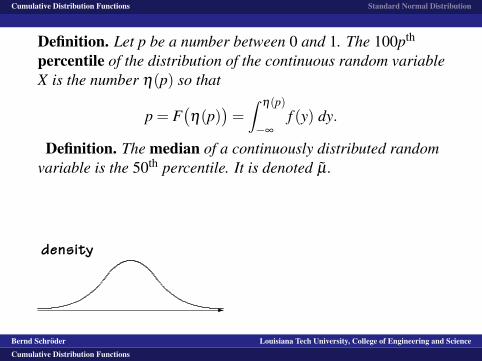
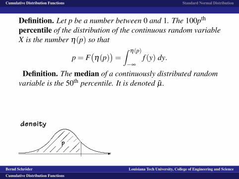
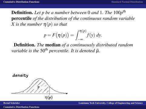
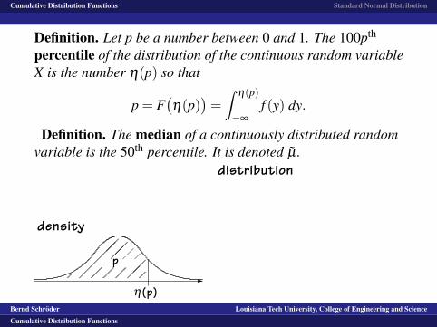
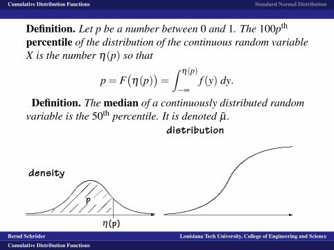
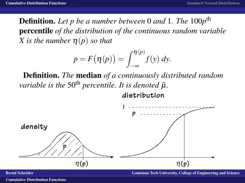
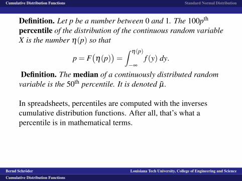
Definition.
Let p be a number between 0 and 1. The 100pth
percentile of the distribution of the continuous random variableX is the number η(p) so that
p = F(η(p)
)=∫
η(p)
−∞
f (y) dy.
Definition. The median of a continuously distributed randomvariable is the 50th percentile. It is denoted µ .
density
-��
��
����p
η(p)
distribution
-
lp
η(p)
Bernd Schroder Louisiana Tech University, College of Engineering and Science
Cumulative Distribution Functions
Cumulative Distribution Functions Standard Normal Distribution
Definition. Let p be a number between 0 and 1.
The 100pth
percentile of the distribution of the continuous random variableX is the number η(p) so that
p = F(η(p)
)=∫
η(p)
−∞
f (y) dy.
Definition. The median of a continuously distributed randomvariable is the 50th percentile. It is denoted µ .
density
-��
��
����p
η(p)
distribution
-
lp
η(p)
Bernd Schroder Louisiana Tech University, College of Engineering and Science
Cumulative Distribution Functions
Cumulative Distribution Functions Standard Normal Distribution
Definition. Let p be a number between 0 and 1. The 100pth
percentile of the distribution of the continuous random variableX is the number η(p) so that
p
= F(η(p)
)=∫
η(p)
−∞
f (y) dy.
Definition. The median of a continuously distributed randomvariable is the 50th percentile. It is denoted µ .
density
-��
��
����p
η(p)
distribution
-
lp
η(p)
Bernd Schroder Louisiana Tech University, College of Engineering and Science
Cumulative Distribution Functions
Cumulative Distribution Functions Standard Normal Distribution
Definition. Let p be a number between 0 and 1. The 100pth
percentile of the distribution of the continuous random variableX is the number η(p) so that
p = F(η(p)
)
=∫
η(p)
−∞
f (y) dy.
Definition. The median of a continuously distributed randomvariable is the 50th percentile. It is denoted µ .
density
-��
��
����p
η(p)
distribution
-
lp
η(p)
Bernd Schroder Louisiana Tech University, College of Engineering and Science
Cumulative Distribution Functions
Cumulative Distribution Functions Standard Normal Distribution
Definition. Let p be a number between 0 and 1. The 100pth
percentile of the distribution of the continuous random variableX is the number η(p) so that
p = F(η(p)
)=∫
η(p)
−∞
f (y) dy.
Definition. The median of a continuously distributed randomvariable is the 50th percentile. It is denoted µ .
density
-��
��
����p
η(p)
distribution
-
lp
η(p)
Bernd Schroder Louisiana Tech University, College of Engineering and Science
Cumulative Distribution Functions
Cumulative Distribution Functions Standard Normal Distribution
Definition. Let p be a number between 0 and 1. The 100pth
percentile of the distribution of the continuous random variableX is the number η(p) so that
p = F(η(p)
)=∫
η(p)
−∞
f (y) dy.
Definition.
The median of a continuously distributed randomvariable is the 50th percentile. It is denoted µ .
density
-��
��
����p
η(p)
distribution
-
lp
η(p)
Bernd Schroder Louisiana Tech University, College of Engineering and Science
Cumulative Distribution Functions
Cumulative Distribution Functions Standard Normal Distribution
Definition. Let p be a number between 0 and 1. The 100pth
percentile of the distribution of the continuous random variableX is the number η(p) so that
p = F(η(p)
)=∫
η(p)
−∞
f (y) dy.
Definition. The median of a continuously distributed randomvariable is the 50th percentile.
It is denoted µ .
density
-��
��
����p
η(p)
distribution
-
lp
η(p)
Bernd Schroder Louisiana Tech University, College of Engineering and Science
Cumulative Distribution Functions
Cumulative Distribution Functions Standard Normal Distribution
Definition. Let p be a number between 0 and 1. The 100pth
percentile of the distribution of the continuous random variableX is the number η(p) so that
p = F(η(p)
)=∫
η(p)
−∞
f (y) dy.
Definition. The median of a continuously distributed randomvariable is the 50th percentile. It is denoted µ .
density
-��
��
����p
η(p)
distribution
-
lp
η(p)
Bernd Schroder Louisiana Tech University, College of Engineering and Science
Cumulative Distribution Functions
Cumulative Distribution Functions Standard Normal Distribution
Definition. Let p be a number between 0 and 1. The 100pth
percentile of the distribution of the continuous random variableX is the number η(p) so that
p = F(η(p)
)=∫
η(p)
−∞
f (y) dy.
Definition. The median of a continuously distributed randomvariable is the 50th percentile. It is denoted µ .
density
-
��
��
����p
η(p)
distribution
-
lp
η(p)
Bernd Schroder Louisiana Tech University, College of Engineering and Science
Cumulative Distribution Functions

Cumulative Distribution Functions Standard Normal Distribution
Definition. Let p be a number between 0 and 1. The 100pth
percentile of the distribution of the continuous random variableX is the number η(p) so that
p = F(η(p)
)=∫
η(p)
−∞
f (y) dy.
Definition. The median of a continuously distributed randomvariable is the 50th percentile. It is denoted µ .
density
-��
��
����
p
η(p)
distribution
-
lp
η(p)
Bernd Schroder Louisiana Tech University, College of Engineering and Science
Cumulative Distribution Functions
Cumulative Distribution Functions Standard Normal Distribution
Definition. Let p be a number between 0 and 1. The 100pth
percentile of the distribution of the continuous random variableX is the number η(p) so that
p = F(η(p)
)=∫
η(p)
−∞
f (y) dy.
Definition. The median of a continuously distributed randomvariable is the 50th percentile. It is denoted µ .
density
-��
��
����p
η(p)
distribution
-
lp
η(p)
Bernd Schroder Louisiana Tech University, College of Engineering and Science
Cumulative Distribution Functions

Cumulative Distribution Functions Standard Normal Distribution
Definition. Let p be a number between 0 and 1. The 100pth
percentile of the distribution of the continuous random variableX is the number η(p) so that
p = F(η(p)
)=∫
η(p)
−∞
f (y) dy.
Definition. The median of a continuously distributed randomvariable is the 50th percentile. It is denoted µ .
density
-��
��
����p
η(p)
distribution
-
l
p
η(p)
Bernd Schroder Louisiana Tech University, College of Engineering and Science
Cumulative Distribution Functions

Cumulative Distribution Functions Standard Normal Distribution
Definition. Let p be a number between 0 and 1. The 100pth
percentile of the distribution of the continuous random variableX is the number η(p) so that
p = F(η(p)
)=∫
η(p)
−∞
f (y) dy.
Definition. The median of a continuously distributed randomvariable is the 50th percentile. It is denoted µ .
density
-��
��
����p
η(p)
distribution
-
lp
η(p)
Bernd Schroder Louisiana Tech University, College of Engineering and Science
Cumulative Distribution Functions

Cumulative Distribution Functions Standard Normal Distribution
Definition. Let p be a number between 0 and 1. The 100pth
percentile of the distribution of the continuous random variableX is the number η(p) so that
p = F(η(p)
)=∫
η(p)
−∞
f (y) dy.
Definition. The median of a continuously distributed randomvariable is the 50th percentile. It is denoted µ .
density
-��
��
����p
η(p)
distribution
-
lp
η(p)
Bernd Schroder Louisiana Tech University, College of Engineering and Science
Cumulative Distribution Functions

Cumulative Distribution Functions Standard Normal Distribution
Definition. Let p be a number between 0 and 1. The 100pth
percentile of the distribution of the continuous random variableX is the number η(p) so that
p = F(η(p)
)=∫
η(p)
−∞
f (y) dy.
Definition. The median of a continuously distributed randomvariable is the 50th percentile. It is denoted µ .
In spreadsheets, percentiles are computed with the inversescumulative distribution functions. After all, that’s what apercentile is in mathematical terms.
Bernd Schroder Louisiana Tech University, College of Engineering and Science
Cumulative Distribution Functions
Cumulative Distribution Functions Standard Normal Distribution
Definition. Let p be a number between 0 and 1. The 100pth
percentile of the distribution of the continuous random variableX is the number η(p) so that
p = F(η(p)
)=∫
η(p)
−∞
f (y) dy.
Definition. The median of a continuously distributed randomvariable is the 50th percentile. It is denoted µ .
In spreadsheets, percentiles are computed with the inversescumulative distribution functions.
After all, that’s what apercentile is in mathematical terms.
Bernd Schroder Louisiana Tech University, College of Engineering and Science
Cumulative Distribution Functions
Cumulative Distribution Functions Standard Normal Distribution
Definition. Let p be a number between 0 and 1. The 100pth
percentile of the distribution of the continuous random variableX is the number η(p) so that
p = F(η(p)
)=∫
η(p)
−∞
f (y) dy.
Definition. The median of a continuously distributed randomvariable is the 50th percentile. It is denoted µ .
In spreadsheets, percentiles are computed with the inversescumulative distribution functions. After all, that’s what apercentile is in mathematical terms.
Bernd Schroder Louisiana Tech University, College of Engineering and Science
Cumulative Distribution Functions

Cumulative Distribution Functions Standard Normal Distribution
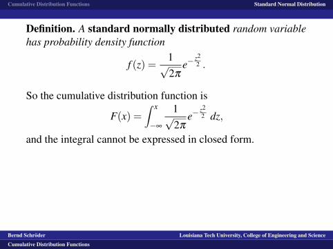
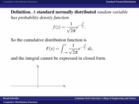
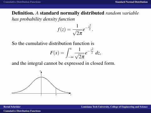
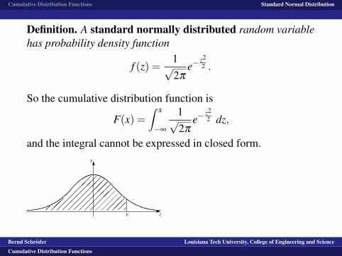
Definition.
A standard normally distributed random variablehas probability density function
f (z) =1√2π
e−z22 .
So the cumulative distribution function is
F(x) =∫ x
−∞
1√2π
e−z22 dz,
and the integral cannot be expressed in closed form.
-z
6y
x���
��
���
����
����
����
����
����
��
Bernd Schroder Louisiana Tech University, College of Engineering and Science
Cumulative Distribution Functions
Cumulative Distribution Functions Standard Normal Distribution
Definition. A standard normally distributed random variablehas probability density function
f (z) =1√2π
e−z22 .
So the cumulative distribution function is
F(x) =∫ x
−∞
1√2π
e−z22 dz
,
and the integral cannot be expressed in closed form.
-z
6y
x���
��
���
����
����
����
����
����
��
Bernd Schroder Louisiana Tech University, College of Engineering and Science
Cumulative Distribution Functions
Cumulative Distribution Functions Standard Normal Distribution
Definition. A standard normally distributed random variablehas probability density function
f (z) =1√2π
e−z22 .
So the cumulative distribution function is
F(x) =∫ x
−∞
1√2π
e−z22 dz,
and the integral cannot be expressed in closed form.
-z
6y
x���
��
���
����
����
����
����
����
��
Bernd Schroder Louisiana Tech University, College of Engineering and Science
Cumulative Distribution Functions
Cumulative Distribution Functions Standard Normal Distribution
Definition. A standard normally distributed random variablehas probability density function
f (z) =1√2π
e−z22 .
So the cumulative distribution function is
F(x) =∫ x
−∞
1√2π
e−z22 dz,
and the integral cannot be expressed in closed form.
-z
6y
x���
��
���
����
����
����
����
����
��
Bernd Schroder Louisiana Tech University, College of Engineering and Science
Cumulative Distribution Functions
Cumulative Distribution Functions Standard Normal Distribution
Definition. A standard normally distributed random variablehas probability density function
f (z) =1√2π
e−z22 .
So the cumulative distribution function is
F(x) =∫ x
−∞
1√2π
e−z22 dz,
and the integral cannot be expressed in closed form.
-z
6y
x
�����
���
����
����
����
����
����
��
Bernd Schroder Louisiana Tech University, College of Engineering and Science
Cumulative Distribution Functions
Cumulative Distribution Functions Standard Normal Distribution
Definition. A standard normally distributed random variablehas probability density function
f (z) =1√2π
e−z22 .
So the cumulative distribution function is
F(x) =∫ x
−∞
1√2π
e−z22 dz,
and the integral cannot be expressed in closed form.
-z
6y
x���
��
���
����
����
����
����
����
��
Bernd Schroder Louisiana Tech University, College of Engineering and Science
Cumulative Distribution Functions
Cumulative Distribution Functions Standard Normal Distribution
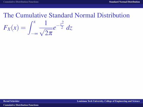
The Cumulative Standard Normal Distribution
FX(x) =∫ x
−∞
1√2π
e−z22 dz
0.00 0.01 0.02 0.03 0.04 0.05 0.06 0.07 0.08 0.090.0 0.5000 0.5040 0.5080 0.5120 0.5160 0.5199 0.5239 0.5279 0.5319 0.53590.1 0.5398 0.5438 0.5478 0.5517 0.5557 0.5596 0.5636 0.5675 0.5714 0.57530.2 0.5793 0.5832 0.5871 0.5910 0.5948 0.5987 0.6026 0.6064 0.6103 0.61410.3 0.6179 0.6217 0.6255 0.6293 0.6331 0.6368 0.6406 0.6443 0.6480 0.65170.4 0.6554 0.6591 0.6628 0.6664 0.6700 0.6736 0.6772 0.6808 0.6844 0.68790.5 0.6915 0.6950 0.6985 0.7019 0.7054 0.7088 0.7123 0.7157 0.7190 0.72240.6 0.7257 0.7291 0.7324 0.7357 0.7389 0.7422 0.7454 0.7486 0.7517 0.75490.7 0.7580 0.7611 0.7642 0.7673 0.7704 0.7734 0.7764 0.7794 0.7823 0.78520.8 0.7881 0.7910 0.7939 0.7967 0.7995 0.8023 0.8051 0.8078 0.8106 0.81330.9 0.8159 0.8186 0.8212 0.8238 0.8264 0.8289 0.8315 0.8340 0.8365 0.83891.0 0.8413 0.8438 0.8461 0.8485 0.8508 0.8531 0.8554 0.8577 0.8599 0.86211.1 0.8643 0.8665 0.8686 0.8708 0.8729 0.8749 0.8770 0.8790 0.8810 0.88301.2 0.8849 0.8869 0.8888 0.8907 0.8925 0.8944 0.8962 0.8980 0.8997 0.90151.3 0.9032 0.9049 0.9066 0.9082 0.9099 0.9115 0.9131 0.9147 0.9162 0.91771.4 0.9192 0.9207 0.9222 0.9236 0.9251 0.9265 0.9279 0.9292 0.9306 0.93191.5 0.9332 0.9345 0.9357 0.9370 0.9382 0.9394 0.9406 0.9418 0.9429 0.94411.6 0.9452 0.9463 0.9474 0.9484 0.9495 0.9505 0.9515 0.9525 0.9535 0.95451.7 0.9554 0.9564 0.9573 0.9582 0.9591 0.9599 0.9608 0.9616 0.9625 0.96331.8 0.9641 0.9649 0.9656 0.9664 0.9671 0.9678 0.9686 0.9693 0.9699 0.97061.9 0.9713 0.9719 0.9726 0.9732 0.9738 0.9744 0.9750 0.9756 0.9761 0.97672.0 0.9772 0.9778 0.9783 0.9788 0.9793 0.9798 0.9803 0.9808 0.9812 0.98172.1 0.9821 0.9826 0.9830 0.9834 0.9838 0.9842 0.9846 0.9850 0.9854 0.98572.2 0.9861 0.9864 0.9868 0.9871 0.9875 0.9878 0.9881 0.9884 0.9887 0.98902.3 0.9893 0.9896 0.9898 0.9901 0.9904 0.9906 0.9909 0.9911 0.9913 0.99162.4 0.9918 0.9920 0.9922 0.9925 0.9927 0.9929 0.9931 0.9932 0.9934 0.99362.5 0.99379 0.99396 0.99413 0.99430 0.99446 0.99461 0.99477 0.99492 0.99506 0.995202.6 0.99534 0.99547 0.99560 0.99573 0.99585 0.99598 0.99609 0.99621 0.99632 0.996432.7 0.99653 0.99664 0.99674 0.99683 0.99693 0.99702 0.99711 0.99720 0.99728 0.997362.8 0.99744 0.99752 0.99760 0.99767 0.99774 0.99781 0.99788 0.99795 0.99801 0.998072.9 0.99813 0.99819 0.99825 0.99831 0.99836 0.99841 0.99846 0.99851 0.99856 0.998613.0 0.99865 0.99869 0.99874 0.99878 0.99882 0.99886 0.99889 0.99893 0.99896 0.99900
Bernd Schroder Louisiana Tech University, College of Engineering and Science
Cumulative Distribution Functions
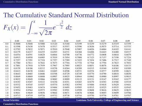
Cumulative Distribution Functions Standard Normal Distribution
The Cumulative Standard Normal Distribution
FX(x) =∫ x
−∞
1√2π
e−z22 dz
A word on spreadsheets and mathematical packages thatprovide distribution functions. Use them. (The table on theprevious panel was made with a spreadsheet.) But make surethe function you use really provides the values you are lookingfor.
Bernd Schroder Louisiana Tech University, College of Engineering and Science
Cumulative Distribution Functions
Cumulative Distribution Functions Standard Normal Distribution
The Cumulative Standard Normal Distribution
FX(x) =∫ x
−∞
1√2π
e−z22 dz
A word on spreadsheets and mathematical packages thatprovide distribution functions.
Use them. (The table on theprevious panel was made with a spreadsheet.) But make surethe function you use really provides the values you are lookingfor.
Bernd Schroder Louisiana Tech University, College of Engineering and Science
Cumulative Distribution Functions
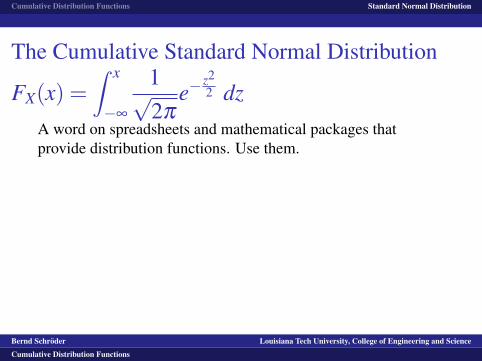
Cumulative Distribution Functions Standard Normal Distribution
The Cumulative Standard Normal Distribution
FX(x) =∫ x
−∞
1√2π
e−z22 dz
A word on spreadsheets and mathematical packages thatprovide distribution functions. Use them.
(The table on theprevious panel was made with a spreadsheet.) But make surethe function you use really provides the values you are lookingfor.
Bernd Schroder Louisiana Tech University, College of Engineering and Science
Cumulative Distribution Functions
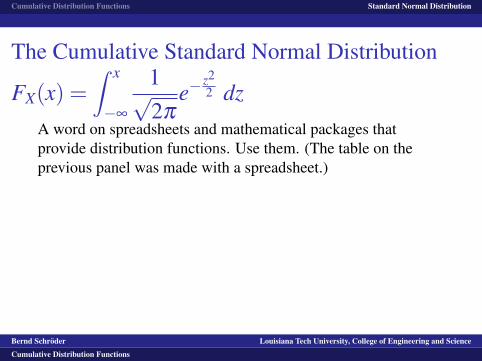
Cumulative Distribution Functions Standard Normal Distribution
The Cumulative Standard Normal Distribution
FX(x) =∫ x
−∞
1√2π
e−z22 dz
A word on spreadsheets and mathematical packages thatprovide distribution functions. Use them. (The table on theprevious panel was made with a spreadsheet.)
But make surethe function you use really provides the values you are lookingfor.
Bernd Schroder Louisiana Tech University, College of Engineering and Science
Cumulative Distribution Functions
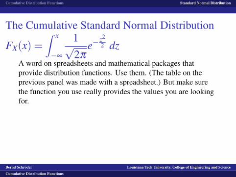
Cumulative Distribution Functions Standard Normal Distribution
The Cumulative Standard Normal Distribution
FX(x) =∫ x
−∞
1√2π
e−z22 dz
A word on spreadsheets and mathematical packages thatprovide distribution functions. Use them. (The table on theprevious panel was made with a spreadsheet.) But make surethe function you use really provides the values you are lookingfor.
Bernd Schroder Louisiana Tech University, College of Engineering and Science
Cumulative Distribution Functions

Cumulative Distribution Functions Standard Normal Distribution
Example.
Let Z be a standard normally distributed randomvariable.P(Z ≤ 1.53) =
0.00 0.01 0.02 0.03 0.04 0.05 0.06 0.07 0.08 0.090.0 0.5000 0.5040 0.5080 0.5120 0.5160 0.5199 0.5239 0.5279 0.5319 0.53590.1 0.5398 0.5438 0.5478 0.5517 0.5557 0.5596 0.5636 0.5675 0.5714 0.57530.2 0.5793 0.5832 0.5871 0.5910 0.5948 0.5987 0.6026 0.6064 0.6103 0.61410.3 0.6179 0.6217 0.6255 0.6293 0.6331 0.6368 0.6406 0.6443 0.6480 0.65170.4 0.6554 0.6591 0.6628 0.6664 0.6700 0.6736 0.6772 0.6808 0.6844 0.68790.5 0.6915 0.6950 0.6985 0.7019 0.7054 0.7088 0.7123 0.7157 0.7190 0.72240.6 0.7257 0.7291 0.7324 0.7357 0.7389 0.7422 0.7454 0.7486 0.7517 0.75490.7 0.7580 0.7611 0.7642 0.7673 0.7704 0.7734 0.7764 0.7794 0.7823 0.78520.8 0.7881 0.7910 0.7939 0.7967 0.7995 0.8023 0.8051 0.8078 0.8106 0.81330.9 0.8159 0.8186 0.8212 0.8238 0.8264 0.8289 0.8315 0.8340 0.8365 0.83891.0 0.8413 0.8438 0.8461 0.8485 0.8508 0.8531 0.8554 0.8577 0.8599 0.86211.1 0.8643 0.8665 0.8686 0.8708 0.8729 0.8749 0.8770 0.8790 0.8810 0.88301.2 0.8849 0.8869 0.8888 0.8907 0.8925 0.8944 0.8962 0.8980 0.8997 0.90151.3 0.9032 0.9049 0.9066 0.9082 0.9099 0.9115 0.9131 0.9147 0.9162 0.91771.4 0.9192 0.9207 0.9222 0.9236 0.9251 0.9265 0.9279 0.9292 0.9306 0.93191.5 0.9332 0.9345 0.9357 0.9370 0.9382 0.9394 0.9406 0.9418 0.9429 0.94411.6 0.9452 0.9463 0.9474 0.9484 0.9495 0.9505 0.9515 0.9525 0.9535 0.95451.7 0.9554 0.9564 0.9573 0.9582 0.9591 0.9599 0.9608 0.9616 0.9625 0.96331.8 0.9641 0.9649 0.9656 0.9664 0.9671 0.9678 0.9686 0.9693 0.9699 0.97061.9 0.9713 0.9719 0.9726 0.9732 0.9738 0.9744 0.9750 0.9756 0.9761 0.97672.0 0.9772 0.9778 0.9783 0.9788 0.9793 0.9798 0.9803 0.9808 0.9812 0.9817
Bernd Schroder Louisiana Tech University, College of Engineering and Science
Cumulative Distribution Functions

Cumulative Distribution Functions Standard Normal Distribution
Example. Let Z be a standard normally distributed randomvariable.
P(Z ≤ 1.53) =0.00 0.01 0.02 0.03 0.04 0.05 0.06 0.07 0.08 0.09
0.0 0.5000 0.5040 0.5080 0.5120 0.5160 0.5199 0.5239 0.5279 0.5319 0.53590.1 0.5398 0.5438 0.5478 0.5517 0.5557 0.5596 0.5636 0.5675 0.5714 0.57530.2 0.5793 0.5832 0.5871 0.5910 0.5948 0.5987 0.6026 0.6064 0.6103 0.61410.3 0.6179 0.6217 0.6255 0.6293 0.6331 0.6368 0.6406 0.6443 0.6480 0.65170.4 0.6554 0.6591 0.6628 0.6664 0.6700 0.6736 0.6772 0.6808 0.6844 0.68790.5 0.6915 0.6950 0.6985 0.7019 0.7054 0.7088 0.7123 0.7157 0.7190 0.72240.6 0.7257 0.7291 0.7324 0.7357 0.7389 0.7422 0.7454 0.7486 0.7517 0.75490.7 0.7580 0.7611 0.7642 0.7673 0.7704 0.7734 0.7764 0.7794 0.7823 0.78520.8 0.7881 0.7910 0.7939 0.7967 0.7995 0.8023 0.8051 0.8078 0.8106 0.81330.9 0.8159 0.8186 0.8212 0.8238 0.8264 0.8289 0.8315 0.8340 0.8365 0.83891.0 0.8413 0.8438 0.8461 0.8485 0.8508 0.8531 0.8554 0.8577 0.8599 0.86211.1 0.8643 0.8665 0.8686 0.8708 0.8729 0.8749 0.8770 0.8790 0.8810 0.88301.2 0.8849 0.8869 0.8888 0.8907 0.8925 0.8944 0.8962 0.8980 0.8997 0.90151.3 0.9032 0.9049 0.9066 0.9082 0.9099 0.9115 0.9131 0.9147 0.9162 0.91771.4 0.9192 0.9207 0.9222 0.9236 0.9251 0.9265 0.9279 0.9292 0.9306 0.93191.5 0.9332 0.9345 0.9357 0.9370 0.9382 0.9394 0.9406 0.9418 0.9429 0.94411.6 0.9452 0.9463 0.9474 0.9484 0.9495 0.9505 0.9515 0.9525 0.9535 0.95451.7 0.9554 0.9564 0.9573 0.9582 0.9591 0.9599 0.9608 0.9616 0.9625 0.96331.8 0.9641 0.9649 0.9656 0.9664 0.9671 0.9678 0.9686 0.9693 0.9699 0.97061.9 0.9713 0.9719 0.9726 0.9732 0.9738 0.9744 0.9750 0.9756 0.9761 0.97672.0 0.9772 0.9778 0.9783 0.9788 0.9793 0.9798 0.9803 0.9808 0.9812 0.9817
Bernd Schroder Louisiana Tech University, College of Engineering and Science
Cumulative Distribution Functions
Cumulative Distribution Functions Standard Normal Distribution
Example. Let Z be a standard normally distributed randomvariable.P(Z ≤ 1.53) =
0.00 0.01 0.02 0.03 0.04 0.05 0.06 0.07 0.08 0.090.0 0.5000 0.5040 0.5080 0.5120 0.5160 0.5199 0.5239 0.5279 0.5319 0.53590.1 0.5398 0.5438 0.5478 0.5517 0.5557 0.5596 0.5636 0.5675 0.5714 0.57530.2 0.5793 0.5832 0.5871 0.5910 0.5948 0.5987 0.6026 0.6064 0.6103 0.61410.3 0.6179 0.6217 0.6255 0.6293 0.6331 0.6368 0.6406 0.6443 0.6480 0.65170.4 0.6554 0.6591 0.6628 0.6664 0.6700 0.6736 0.6772 0.6808 0.6844 0.68790.5 0.6915 0.6950 0.6985 0.7019 0.7054 0.7088 0.7123 0.7157 0.7190 0.72240.6 0.7257 0.7291 0.7324 0.7357 0.7389 0.7422 0.7454 0.7486 0.7517 0.75490.7 0.7580 0.7611 0.7642 0.7673 0.7704 0.7734 0.7764 0.7794 0.7823 0.78520.8 0.7881 0.7910 0.7939 0.7967 0.7995 0.8023 0.8051 0.8078 0.8106 0.81330.9 0.8159 0.8186 0.8212 0.8238 0.8264 0.8289 0.8315 0.8340 0.8365 0.83891.0 0.8413 0.8438 0.8461 0.8485 0.8508 0.8531 0.8554 0.8577 0.8599 0.86211.1 0.8643 0.8665 0.8686 0.8708 0.8729 0.8749 0.8770 0.8790 0.8810 0.88301.2 0.8849 0.8869 0.8888 0.8907 0.8925 0.8944 0.8962 0.8980 0.8997 0.90151.3 0.9032 0.9049 0.9066 0.9082 0.9099 0.9115 0.9131 0.9147 0.9162 0.91771.4 0.9192 0.9207 0.9222 0.9236 0.9251 0.9265 0.9279 0.9292 0.9306 0.93191.5 0.9332 0.9345 0.9357 0.9370 0.9382 0.9394 0.9406 0.9418 0.9429 0.94411.6 0.9452 0.9463 0.9474 0.9484 0.9495 0.9505 0.9515 0.9525 0.9535 0.95451.7 0.9554 0.9564 0.9573 0.9582 0.9591 0.9599 0.9608 0.9616 0.9625 0.96331.8 0.9641 0.9649 0.9656 0.9664 0.9671 0.9678 0.9686 0.9693 0.9699 0.97061.9 0.9713 0.9719 0.9726 0.9732 0.9738 0.9744 0.9750 0.9756 0.9761 0.97672.0 0.9772 0.9778 0.9783 0.9788 0.9793 0.9798 0.9803 0.9808 0.9812 0.9817
Bernd Schroder Louisiana Tech University, College of Engineering and Science
Cumulative Distribution Functions
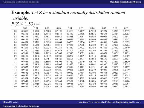
Cumulative Distribution Functions Standard Normal Distribution
Example. Let Z be a standard normally distributed randomvariable.P(Z ≤ 1.53) =
0.00 0.01 0.02 0.03 0.04 0.05 0.06 0.07 0.08 0.090.0 0.5000 0.5040 0.5080 0.5120 0.5160 0.5199 0.5239 0.5279 0.5319 0.53590.1 0.5398 0.5438 0.5478 0.5517 0.5557 0.5596 0.5636 0.5675 0.5714 0.57530.2 0.5793 0.5832 0.5871 0.5910 0.5948 0.5987 0.6026 0.6064 0.6103 0.61410.3 0.6179 0.6217 0.6255 0.6293 0.6331 0.6368 0.6406 0.6443 0.6480 0.65170.4 0.6554 0.6591 0.6628 0.6664 0.6700 0.6736 0.6772 0.6808 0.6844 0.68790.5 0.6915 0.6950 0.6985 0.7019 0.7054 0.7088 0.7123 0.7157 0.7190 0.72240.6 0.7257 0.7291 0.7324 0.7357 0.7389 0.7422 0.7454 0.7486 0.7517 0.75490.7 0.7580 0.7611 0.7642 0.7673 0.7704 0.7734 0.7764 0.7794 0.7823 0.78520.8 0.7881 0.7910 0.7939 0.7967 0.7995 0.8023 0.8051 0.8078 0.8106 0.81330.9 0.8159 0.8186 0.8212 0.8238 0.8264 0.8289 0.8315 0.8340 0.8365 0.83891.0 0.8413 0.8438 0.8461 0.8485 0.8508 0.8531 0.8554 0.8577 0.8599 0.86211.1 0.8643 0.8665 0.8686 0.8708 0.8729 0.8749 0.8770 0.8790 0.8810 0.88301.2 0.8849 0.8869 0.8888 0.8907 0.8925 0.8944 0.8962 0.8980 0.8997 0.90151.3 0.9032 0.9049 0.9066 0.9082 0.9099 0.9115 0.9131 0.9147 0.9162 0.91771.4 0.9192 0.9207 0.9222 0.9236 0.9251 0.9265 0.9279 0.9292 0.9306 0.93191.5 0.9332 0.9345 0.9357 0.9370 0.9382 0.9394 0.9406 0.9418 0.9429 0.94411.6 0.9452 0.9463 0.9474 0.9484 0.9495 0.9505 0.9515 0.9525 0.9535 0.95451.7 0.9554 0.9564 0.9573 0.9582 0.9591 0.9599 0.9608 0.9616 0.9625 0.96331.8 0.9641 0.9649 0.9656 0.9664 0.9671 0.9678 0.9686 0.9693 0.9699 0.97061.9 0.9713 0.9719 0.9726 0.9732 0.9738 0.9744 0.9750 0.9756 0.9761 0.97672.0 0.9772 0.9778 0.9783 0.9788 0.9793 0.9798 0.9803 0.9808 0.9812 0.9817
Bernd Schroder Louisiana Tech University, College of Engineering and Science
Cumulative Distribution Functions
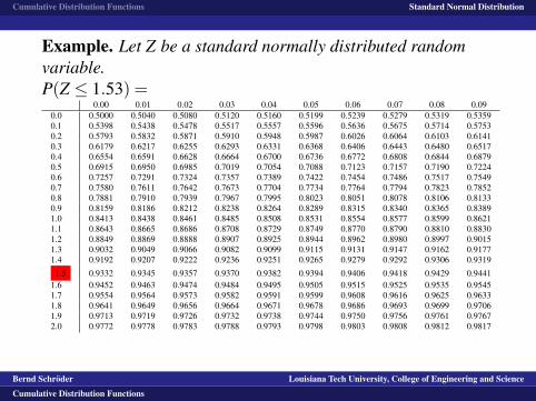
Cumulative Distribution Functions Standard Normal Distribution
Example. Let Z be a standard normally distributed randomvariable.P(Z ≤ 1.53) =
0.00 0.01 0.02 0.03 0.04 0.05 0.06 0.07 0.08 0.090.0 0.5000 0.5040 0.5080 0.5120 0.5160 0.5199 0.5239 0.5279 0.5319 0.53590.1 0.5398 0.5438 0.5478 0.5517 0.5557 0.5596 0.5636 0.5675 0.5714 0.57530.2 0.5793 0.5832 0.5871 0.5910 0.5948 0.5987 0.6026 0.6064 0.6103 0.61410.3 0.6179 0.6217 0.6255 0.6293 0.6331 0.6368 0.6406 0.6443 0.6480 0.65170.4 0.6554 0.6591 0.6628 0.6664 0.6700 0.6736 0.6772 0.6808 0.6844 0.68790.5 0.6915 0.6950 0.6985 0.7019 0.7054 0.7088 0.7123 0.7157 0.7190 0.72240.6 0.7257 0.7291 0.7324 0.7357 0.7389 0.7422 0.7454 0.7486 0.7517 0.75490.7 0.7580 0.7611 0.7642 0.7673 0.7704 0.7734 0.7764 0.7794 0.7823 0.78520.8 0.7881 0.7910 0.7939 0.7967 0.7995 0.8023 0.8051 0.8078 0.8106 0.81330.9 0.8159 0.8186 0.8212 0.8238 0.8264 0.8289 0.8315 0.8340 0.8365 0.83891.0 0.8413 0.8438 0.8461 0.8485 0.8508 0.8531 0.8554 0.8577 0.8599 0.86211.1 0.8643 0.8665 0.8686 0.8708 0.8729 0.8749 0.8770 0.8790 0.8810 0.88301.2 0.8849 0.8869 0.8888 0.8907 0.8925 0.8944 0.8962 0.8980 0.8997 0.90151.3 0.9032 0.9049 0.9066 0.9082 0.9099 0.9115 0.9131 0.9147 0.9162 0.91771.4 0.9192 0.9207 0.9222 0.9236 0.9251 0.9265 0.9279 0.9292 0.9306 0.9319
1.5 0.9332 0.9345 0.9357 0.9370 0.9382 0.9394 0.9406 0.9418 0.9429 0.94411.6 0.9452 0.9463 0.9474 0.9484 0.9495 0.9505 0.9515 0.9525 0.9535 0.95451.7 0.9554 0.9564 0.9573 0.9582 0.9591 0.9599 0.9608 0.9616 0.9625 0.96331.8 0.9641 0.9649 0.9656 0.9664 0.9671 0.9678 0.9686 0.9693 0.9699 0.97061.9 0.9713 0.9719 0.9726 0.9732 0.9738 0.9744 0.9750 0.9756 0.9761 0.97672.0 0.9772 0.9778 0.9783 0.9788 0.9793 0.9798 0.9803 0.9808 0.9812 0.9817
Bernd Schroder Louisiana Tech University, College of Engineering and Science
Cumulative Distribution Functions
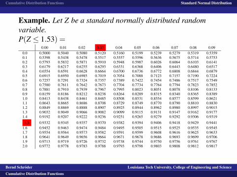
Cumulative Distribution Functions Standard Normal Distribution
Example. Let Z be a standard normally distributed randomvariable.P(Z ≤ 1.53) =
0.00 0.01 0.02 0.03 0.04 0.05 0.06 0.07 0.08 0.090.0 0.5000 0.5040 0.5080 0.5120 0.5160 0.5199 0.5239 0.5279 0.5319 0.53590.1 0.5398 0.5438 0.5478 0.5517 0.5557 0.5596 0.5636 0.5675 0.5714 0.57530.2 0.5793 0.5832 0.5871 0.5910 0.5948 0.5987 0.6026 0.6064 0.6103 0.61410.3 0.6179 0.6217 0.6255 0.6293 0.6331 0.6368 0.6406 0.6443 0.6480 0.65170.4 0.6554 0.6591 0.6628 0.6664 0.6700 0.6736 0.6772 0.6808 0.6844 0.68790.5 0.6915 0.6950 0.6985 0.7019 0.7054 0.7088 0.7123 0.7157 0.7190 0.72240.6 0.7257 0.7291 0.7324 0.7357 0.7389 0.7422 0.7454 0.7486 0.7517 0.75490.7 0.7580 0.7611 0.7642 0.7673 0.7704 0.7734 0.7764 0.7794 0.7823 0.78520.8 0.7881 0.7910 0.7939 0.7967 0.7995 0.8023 0.8051 0.8078 0.8106 0.81330.9 0.8159 0.8186 0.8212 0.8238 0.8264 0.8289 0.8315 0.8340 0.8365 0.83891.0 0.8413 0.8438 0.8461 0.8485 0.8508 0.8531 0.8554 0.8577 0.8599 0.86211.1 0.8643 0.8665 0.8686 0.8708 0.8729 0.8749 0.8770 0.8790 0.8810 0.88301.2 0.8849 0.8869 0.8888 0.8907 0.8925 0.8944 0.8962 0.8980 0.8997 0.90151.3 0.9032 0.9049 0.9066 0.9082 0.9099 0.9115 0.9131 0.9147 0.9162 0.91771.4 0.9192 0.9207 0.9222 0.9236 0.9251 0.9265 0.9279 0.9292 0.9306 0.9319
1.5 0.9332 0.9345 0.9357 0.9370 0.9382 0.9394 0.9406 0.9418 0.9429 0.94411.6 0.9452 0.9463 0.9474 0.9484 0.9495 0.9505 0.9515 0.9525 0.9535 0.95451.7 0.9554 0.9564 0.9573 0.9582 0.9591 0.9599 0.9608 0.9616 0.9625 0.96331.8 0.9641 0.9649 0.9656 0.9664 0.9671 0.9678 0.9686 0.9693 0.9699 0.97061.9 0.9713 0.9719 0.9726 0.9732 0.9738 0.9744 0.9750 0.9756 0.9761 0.97672.0 0.9772 0.9778 0.9783 0.9788 0.9793 0.9798 0.9803 0.9808 0.9812 0.9817
Bernd Schroder Louisiana Tech University, College of Engineering and Science
Cumulative Distribution Functions
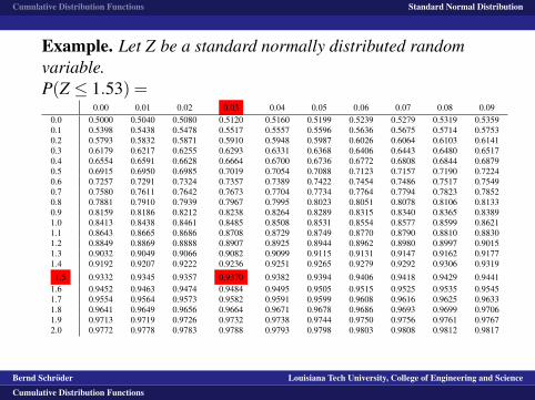
Cumulative Distribution Functions Standard Normal Distribution
Example. Let Z be a standard normally distributed randomvariable.P(Z ≤ 1.53) =
0.00 0.01 0.02 0.03 0.04 0.05 0.06 0.07 0.08 0.090.0 0.5000 0.5040 0.5080 0.5120 0.5160 0.5199 0.5239 0.5279 0.5319 0.53590.1 0.5398 0.5438 0.5478 0.5517 0.5557 0.5596 0.5636 0.5675 0.5714 0.57530.2 0.5793 0.5832 0.5871 0.5910 0.5948 0.5987 0.6026 0.6064 0.6103 0.61410.3 0.6179 0.6217 0.6255 0.6293 0.6331 0.6368 0.6406 0.6443 0.6480 0.65170.4 0.6554 0.6591 0.6628 0.6664 0.6700 0.6736 0.6772 0.6808 0.6844 0.68790.5 0.6915 0.6950 0.6985 0.7019 0.7054 0.7088 0.7123 0.7157 0.7190 0.72240.6 0.7257 0.7291 0.7324 0.7357 0.7389 0.7422 0.7454 0.7486 0.7517 0.75490.7 0.7580 0.7611 0.7642 0.7673 0.7704 0.7734 0.7764 0.7794 0.7823 0.78520.8 0.7881 0.7910 0.7939 0.7967 0.7995 0.8023 0.8051 0.8078 0.8106 0.81330.9 0.8159 0.8186 0.8212 0.8238 0.8264 0.8289 0.8315 0.8340 0.8365 0.83891.0 0.8413 0.8438 0.8461 0.8485 0.8508 0.8531 0.8554 0.8577 0.8599 0.86211.1 0.8643 0.8665 0.8686 0.8708 0.8729 0.8749 0.8770 0.8790 0.8810 0.88301.2 0.8849 0.8869 0.8888 0.8907 0.8925 0.8944 0.8962 0.8980 0.8997 0.90151.3 0.9032 0.9049 0.9066 0.9082 0.9099 0.9115 0.9131 0.9147 0.9162 0.91771.4 0.9192 0.9207 0.9222 0.9236 0.9251 0.9265 0.9279 0.9292 0.9306 0.9319
1.5 0.9332 0.9345 0.9357 0.9370 0.9382 0.9394 0.9406 0.9418 0.9429 0.94411.6 0.9452 0.9463 0.9474 0.9484 0.9495 0.9505 0.9515 0.9525 0.9535 0.95451.7 0.9554 0.9564 0.9573 0.9582 0.9591 0.9599 0.9608 0.9616 0.9625 0.96331.8 0.9641 0.9649 0.9656 0.9664 0.9671 0.9678 0.9686 0.9693 0.9699 0.97061.9 0.9713 0.9719 0.9726 0.9732 0.9738 0.9744 0.9750 0.9756 0.9761 0.97672.0 0.9772 0.9778 0.9783 0.9788 0.9793 0.9798 0.9803 0.9808 0.9812 0.9817
Bernd Schroder Louisiana Tech University, College of Engineering and Science
Cumulative Distribution Functions
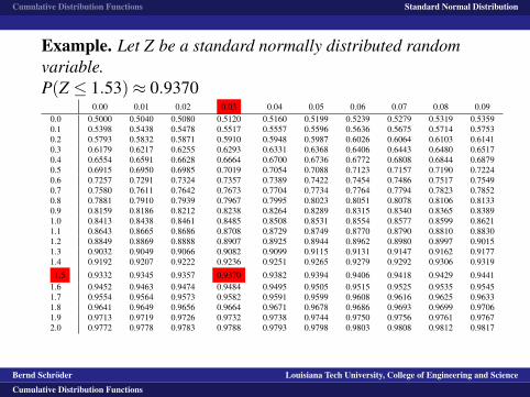
Cumulative Distribution Functions Standard Normal Distribution
Example. Let Z be a standard normally distributed randomvariable.P(Z ≤ 1.53)≈ 0.9370
0.00 0.01 0.02 0.03 0.04 0.05 0.06 0.07 0.08 0.090.0 0.5000 0.5040 0.5080 0.5120 0.5160 0.5199 0.5239 0.5279 0.5319 0.53590.1 0.5398 0.5438 0.5478 0.5517 0.5557 0.5596 0.5636 0.5675 0.5714 0.57530.2 0.5793 0.5832 0.5871 0.5910 0.5948 0.5987 0.6026 0.6064 0.6103 0.61410.3 0.6179 0.6217 0.6255 0.6293 0.6331 0.6368 0.6406 0.6443 0.6480 0.65170.4 0.6554 0.6591 0.6628 0.6664 0.6700 0.6736 0.6772 0.6808 0.6844 0.68790.5 0.6915 0.6950 0.6985 0.7019 0.7054 0.7088 0.7123 0.7157 0.7190 0.72240.6 0.7257 0.7291 0.7324 0.7357 0.7389 0.7422 0.7454 0.7486 0.7517 0.75490.7 0.7580 0.7611 0.7642 0.7673 0.7704 0.7734 0.7764 0.7794 0.7823 0.78520.8 0.7881 0.7910 0.7939 0.7967 0.7995 0.8023 0.8051 0.8078 0.8106 0.81330.9 0.8159 0.8186 0.8212 0.8238 0.8264 0.8289 0.8315 0.8340 0.8365 0.83891.0 0.8413 0.8438 0.8461 0.8485 0.8508 0.8531 0.8554 0.8577 0.8599 0.86211.1 0.8643 0.8665 0.8686 0.8708 0.8729 0.8749 0.8770 0.8790 0.8810 0.88301.2 0.8849 0.8869 0.8888 0.8907 0.8925 0.8944 0.8962 0.8980 0.8997 0.90151.3 0.9032 0.9049 0.9066 0.9082 0.9099 0.9115 0.9131 0.9147 0.9162 0.91771.4 0.9192 0.9207 0.9222 0.9236 0.9251 0.9265 0.9279 0.9292 0.9306 0.9319
1.5 0.9332 0.9345 0.9357 0.9370 0.9382 0.9394 0.9406 0.9418 0.9429 0.94411.6 0.9452 0.9463 0.9474 0.9484 0.9495 0.9505 0.9515 0.9525 0.9535 0.95451.7 0.9554 0.9564 0.9573 0.9582 0.9591 0.9599 0.9608 0.9616 0.9625 0.96331.8 0.9641 0.9649 0.9656 0.9664 0.9671 0.9678 0.9686 0.9693 0.9699 0.97061.9 0.9713 0.9719 0.9726 0.9732 0.9738 0.9744 0.9750 0.9756 0.9761 0.97672.0 0.9772 0.9778 0.9783 0.9788 0.9793 0.9798 0.9803 0.9808 0.9812 0.9817
Duh.
Bernd Schroder Louisiana Tech University, College of Engineering and Science
Cumulative Distribution Functions
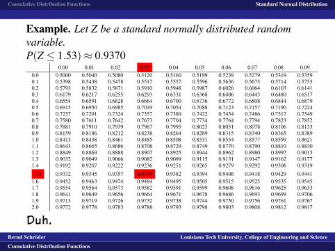
Cumulative Distribution Functions Standard Normal Distribution
Example. Let Z be a standard normally distributed randomvariable.P(Z ≤ 1.53)≈ 0.9370
0.00 0.01 0.02 0.03 0.04 0.05 0.06 0.07 0.08 0.090.0 0.5000 0.5040 0.5080 0.5120 0.5160 0.5199 0.5239 0.5279 0.5319 0.53590.1 0.5398 0.5438 0.5478 0.5517 0.5557 0.5596 0.5636 0.5675 0.5714 0.57530.2 0.5793 0.5832 0.5871 0.5910 0.5948 0.5987 0.6026 0.6064 0.6103 0.61410.3 0.6179 0.6217 0.6255 0.6293 0.6331 0.6368 0.6406 0.6443 0.6480 0.65170.4 0.6554 0.6591 0.6628 0.6664 0.6700 0.6736 0.6772 0.6808 0.6844 0.68790.5 0.6915 0.6950 0.6985 0.7019 0.7054 0.7088 0.7123 0.7157 0.7190 0.72240.6 0.7257 0.7291 0.7324 0.7357 0.7389 0.7422 0.7454 0.7486 0.7517 0.75490.7 0.7580 0.7611 0.7642 0.7673 0.7704 0.7734 0.7764 0.7794 0.7823 0.78520.8 0.7881 0.7910 0.7939 0.7967 0.7995 0.8023 0.8051 0.8078 0.8106 0.81330.9 0.8159 0.8186 0.8212 0.8238 0.8264 0.8289 0.8315 0.8340 0.8365 0.83891.0 0.8413 0.8438 0.8461 0.8485 0.8508 0.8531 0.8554 0.8577 0.8599 0.86211.1 0.8643 0.8665 0.8686 0.8708 0.8729 0.8749 0.8770 0.8790 0.8810 0.88301.2 0.8849 0.8869 0.8888 0.8907 0.8925 0.8944 0.8962 0.8980 0.8997 0.90151.3 0.9032 0.9049 0.9066 0.9082 0.9099 0.9115 0.9131 0.9147 0.9162 0.91771.4 0.9192 0.9207 0.9222 0.9236 0.9251 0.9265 0.9279 0.9292 0.9306 0.9319
1.5 0.9332 0.9345 0.9357 0.9370 0.9382 0.9394 0.9406 0.9418 0.9429 0.94411.6 0.9452 0.9463 0.9474 0.9484 0.9495 0.9505 0.9515 0.9525 0.9535 0.95451.7 0.9554 0.9564 0.9573 0.9582 0.9591 0.9599 0.9608 0.9616 0.9625 0.96331.8 0.9641 0.9649 0.9656 0.9664 0.9671 0.9678 0.9686 0.9693 0.9699 0.97061.9 0.9713 0.9719 0.9726 0.9732 0.9738 0.9744 0.9750 0.9756 0.9761 0.97672.0 0.9772 0.9778 0.9783 0.9788 0.9793 0.9798 0.9803 0.9808 0.9812 0.9817
Duh.Bernd Schroder Louisiana Tech University, College of Engineering and Science
Cumulative Distribution Functions

Cumulative Distribution Functions Standard Normal Distribution
Example. Let Z be a standard normally distributed randomvariable.
Find P(Z > 0.78).0.00 0.01 0.02 0.03 0.04 0.05 0.06 0.07 0.08 0.09
0.0 0.5000 0.5040 0.5080 0.5120 0.5160 0.5199 0.5239 0.5279 0.5319 0.53590.1 0.5398 0.5438 0.5478 0.5517 0.5557 0.5596 0.5636 0.5675 0.5714 0.57530.2 0.5793 0.5832 0.5871 0.5910 0.5948 0.5987 0.6026 0.6064 0.6103 0.61410.3 0.6179 0.6217 0.6255 0.6293 0.6331 0.6368 0.6406 0.6443 0.6480 0.65170.4 0.6554 0.6591 0.6628 0.6664 0.6700 0.6736 0.6772 0.6808 0.6844 0.68790.5 0.6915 0.6950 0.6985 0.7019 0.7054 0.7088 0.7123 0.7157 0.7190 0.72240.6 0.7257 0.7291 0.7324 0.7357 0.7389 0.7422 0.7454 0.7486 0.7517 0.75490.7 0.7580 0.7611 0.7642 0.7673 0.7704 0.7734 0.7764 0.7794 0.7823 0.78520.8 0.7881 0.7910 0.7939 0.7967 0.7995 0.8023 0.8051 0.8078 0.8106 0.81330.9 0.8159 0.8186 0.8212 0.8238 0.8264 0.8289 0.8315 0.8340 0.8365 0.83891.0 0.8413 0.8438 0.8461 0.8485 0.8508 0.8531 0.8554 0.8577 0.8599 0.86211.1 0.8643 0.8665 0.8686 0.8708 0.8729 0.8749 0.8770 0.8790 0.8810 0.88301.2 0.8849 0.8869 0.8888 0.8907 0.8925 0.8944 0.8962 0.8980 0.8997 0.90151.3 0.9032 0.9049 0.9066 0.9082 0.9099 0.9115 0.9131 0.9147 0.9162 0.91771.4 0.9192 0.9207 0.9222 0.9236 0.9251 0.9265 0.9279 0.9292 0.9306 0.93191.5 0.9332 0.9345 0.9357 0.9370 0.9382 0.9394 0.9406 0.9418 0.9429 0.94411.6 0.9452 0.9463 0.9474 0.9484 0.9495 0.9505 0.9515 0.9525 0.9535 0.95451.7 0.9554 0.9564 0.9573 0.9582 0.9591 0.9599 0.9608 0.9616 0.9625 0.96331.8 0.9641 0.9649 0.9656 0.9664 0.9671 0.9678 0.9686 0.9693 0.9699 0.97061.9 0.9713 0.9719 0.9726 0.9732 0.9738 0.9744 0.9750 0.9756 0.9761 0.97672.0 0.9772 0.9778 0.9783 0.9788 0.9793 0.9798 0.9803 0.9808 0.9812 0.9817
Bernd Schroder Louisiana Tech University, College of Engineering and Science
Cumulative Distribution Functions
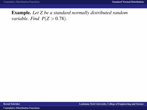
Cumulative Distribution Functions Standard Normal Distribution
Example. Let Z be a standard normally distributed randomvariable. Find P(Z > 0.78).
0.00 0.01 0.02 0.03 0.04 0.05 0.06 0.07 0.08 0.090.0 0.5000 0.5040 0.5080 0.5120 0.5160 0.5199 0.5239 0.5279 0.5319 0.53590.1 0.5398 0.5438 0.5478 0.5517 0.5557 0.5596 0.5636 0.5675 0.5714 0.57530.2 0.5793 0.5832 0.5871 0.5910 0.5948 0.5987 0.6026 0.6064 0.6103 0.61410.3 0.6179 0.6217 0.6255 0.6293 0.6331 0.6368 0.6406 0.6443 0.6480 0.65170.4 0.6554 0.6591 0.6628 0.6664 0.6700 0.6736 0.6772 0.6808 0.6844 0.68790.5 0.6915 0.6950 0.6985 0.7019 0.7054 0.7088 0.7123 0.7157 0.7190 0.72240.6 0.7257 0.7291 0.7324 0.7357 0.7389 0.7422 0.7454 0.7486 0.7517 0.75490.7 0.7580 0.7611 0.7642 0.7673 0.7704 0.7734 0.7764 0.7794 0.7823 0.78520.8 0.7881 0.7910 0.7939 0.7967 0.7995 0.8023 0.8051 0.8078 0.8106 0.81330.9 0.8159 0.8186 0.8212 0.8238 0.8264 0.8289 0.8315 0.8340 0.8365 0.83891.0 0.8413 0.8438 0.8461 0.8485 0.8508 0.8531 0.8554 0.8577 0.8599 0.86211.1 0.8643 0.8665 0.8686 0.8708 0.8729 0.8749 0.8770 0.8790 0.8810 0.88301.2 0.8849 0.8869 0.8888 0.8907 0.8925 0.8944 0.8962 0.8980 0.8997 0.90151.3 0.9032 0.9049 0.9066 0.9082 0.9099 0.9115 0.9131 0.9147 0.9162 0.91771.4 0.9192 0.9207 0.9222 0.9236 0.9251 0.9265 0.9279 0.9292 0.9306 0.93191.5 0.9332 0.9345 0.9357 0.9370 0.9382 0.9394 0.9406 0.9418 0.9429 0.94411.6 0.9452 0.9463 0.9474 0.9484 0.9495 0.9505 0.9515 0.9525 0.9535 0.95451.7 0.9554 0.9564 0.9573 0.9582 0.9591 0.9599 0.9608 0.9616 0.9625 0.96331.8 0.9641 0.9649 0.9656 0.9664 0.9671 0.9678 0.9686 0.9693 0.9699 0.97061.9 0.9713 0.9719 0.9726 0.9732 0.9738 0.9744 0.9750 0.9756 0.9761 0.97672.0 0.9772 0.9778 0.9783 0.9788 0.9793 0.9798 0.9803 0.9808 0.9812 0.9817
Bernd Schroder Louisiana Tech University, College of Engineering and Science
Cumulative Distribution Functions
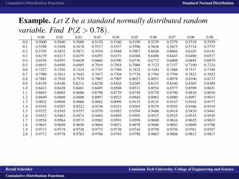
Cumulative Distribution Functions Standard Normal Distribution
Example. Let Z be a standard normally distributed randomvariable. Find P(Z > 0.78).
0.00 0.01 0.02 0.03 0.04 0.05 0.06 0.07 0.08 0.090.0 0.5000 0.5040 0.5080 0.5120 0.5160 0.5199 0.5239 0.5279 0.5319 0.53590.1 0.5398 0.5438 0.5478 0.5517 0.5557 0.5596 0.5636 0.5675 0.5714 0.57530.2 0.5793 0.5832 0.5871 0.5910 0.5948 0.5987 0.6026 0.6064 0.6103 0.61410.3 0.6179 0.6217 0.6255 0.6293 0.6331 0.6368 0.6406 0.6443 0.6480 0.65170.4 0.6554 0.6591 0.6628 0.6664 0.6700 0.6736 0.6772 0.6808 0.6844 0.68790.5 0.6915 0.6950 0.6985 0.7019 0.7054 0.7088 0.7123 0.7157 0.7190 0.72240.6 0.7257 0.7291 0.7324 0.7357 0.7389 0.7422 0.7454 0.7486 0.7517 0.75490.7 0.7580 0.7611 0.7642 0.7673 0.7704 0.7734 0.7764 0.7794 0.7823 0.78520.8 0.7881 0.7910 0.7939 0.7967 0.7995 0.8023 0.8051 0.8078 0.8106 0.81330.9 0.8159 0.8186 0.8212 0.8238 0.8264 0.8289 0.8315 0.8340 0.8365 0.83891.0 0.8413 0.8438 0.8461 0.8485 0.8508 0.8531 0.8554 0.8577 0.8599 0.86211.1 0.8643 0.8665 0.8686 0.8708 0.8729 0.8749 0.8770 0.8790 0.8810 0.88301.2 0.8849 0.8869 0.8888 0.8907 0.8925 0.8944 0.8962 0.8980 0.8997 0.90151.3 0.9032 0.9049 0.9066 0.9082 0.9099 0.9115 0.9131 0.9147 0.9162 0.91771.4 0.9192 0.9207 0.9222 0.9236 0.9251 0.9265 0.9279 0.9292 0.9306 0.93191.5 0.9332 0.9345 0.9357 0.9370 0.9382 0.9394 0.9406 0.9418 0.9429 0.94411.6 0.9452 0.9463 0.9474 0.9484 0.9495 0.9505 0.9515 0.9525 0.9535 0.95451.7 0.9554 0.9564 0.9573 0.9582 0.9591 0.9599 0.9608 0.9616 0.9625 0.96331.8 0.9641 0.9649 0.9656 0.9664 0.9671 0.9678 0.9686 0.9693 0.9699 0.97061.9 0.9713 0.9719 0.9726 0.9732 0.9738 0.9744 0.9750 0.9756 0.9761 0.97672.0 0.9772 0.9778 0.9783 0.9788 0.9793 0.9798 0.9803 0.9808 0.9812 0.9817
Bernd Schroder Louisiana Tech University, College of Engineering and Science
Cumulative Distribution Functions
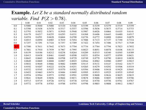
Cumulative Distribution Functions Standard Normal Distribution
Example. Let Z be a standard normally distributed randomvariable. Find P(Z > 0.78).
0.00 0.01 0.02 0.03 0.04 0.05 0.06 0.07 0.08 0.090.0 0.5000 0.5040 0.5080 0.5120 0.5160 0.5199 0.5239 0.5279 0.5319 0.53590.1 0.5398 0.5438 0.5478 0.5517 0.5557 0.5596 0.5636 0.5675 0.5714 0.57530.2 0.5793 0.5832 0.5871 0.5910 0.5948 0.5987 0.6026 0.6064 0.6103 0.61410.3 0.6179 0.6217 0.6255 0.6293 0.6331 0.6368 0.6406 0.6443 0.6480 0.65170.4 0.6554 0.6591 0.6628 0.6664 0.6700 0.6736 0.6772 0.6808 0.6844 0.68790.5 0.6915 0.6950 0.6985 0.7019 0.7054 0.7088 0.7123 0.7157 0.7190 0.72240.6 0.7257 0.7291 0.7324 0.7357 0.7389 0.7422 0.7454 0.7486 0.7517 0.7549
0.7 0.7580 0.7611 0.7642 0.7673 0.7704 0.7734 0.7764 0.7794 0.7823 0.78520.8 0.7881 0.7910 0.7939 0.7967 0.7995 0.8023 0.8051 0.8078 0.8106 0.81330.9 0.8159 0.8186 0.8212 0.8238 0.8264 0.8289 0.8315 0.8340 0.8365 0.83891.0 0.8413 0.8438 0.8461 0.8485 0.8508 0.8531 0.8554 0.8577 0.8599 0.86211.1 0.8643 0.8665 0.8686 0.8708 0.8729 0.8749 0.8770 0.8790 0.8810 0.88301.2 0.8849 0.8869 0.8888 0.8907 0.8925 0.8944 0.8962 0.8980 0.8997 0.90151.3 0.9032 0.9049 0.9066 0.9082 0.9099 0.9115 0.9131 0.9147 0.9162 0.91771.4 0.9192 0.9207 0.9222 0.9236 0.9251 0.9265 0.9279 0.9292 0.9306 0.93191.5 0.9332 0.9345 0.9357 0.9370 0.9382 0.9394 0.9406 0.9418 0.9429 0.94411.6 0.9452 0.9463 0.9474 0.9484 0.9495 0.9505 0.9515 0.9525 0.9535 0.95451.7 0.9554 0.9564 0.9573 0.9582 0.9591 0.9599 0.9608 0.9616 0.9625 0.96331.8 0.9641 0.9649 0.9656 0.9664 0.9671 0.9678 0.9686 0.9693 0.9699 0.97061.9 0.9713 0.9719 0.9726 0.9732 0.9738 0.9744 0.9750 0.9756 0.9761 0.97672.0 0.9772 0.9778 0.9783 0.9788 0.9793 0.9798 0.9803 0.9808 0.9812 0.9817
Bernd Schroder Louisiana Tech University, College of Engineering and Science
Cumulative Distribution Functions
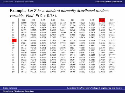
Cumulative Distribution Functions Standard Normal Distribution
Example. Let Z be a standard normally distributed randomvariable. Find P(Z > 0.78).
0.00 0.01 0.02 0.03 0.04 0.05 0.06 0.07 0.08 0.090.0 0.5000 0.5040 0.5080 0.5120 0.5160 0.5199 0.5239 0.5279 0.5319 0.53590.1 0.5398 0.5438 0.5478 0.5517 0.5557 0.5596 0.5636 0.5675 0.5714 0.57530.2 0.5793 0.5832 0.5871 0.5910 0.5948 0.5987 0.6026 0.6064 0.6103 0.61410.3 0.6179 0.6217 0.6255 0.6293 0.6331 0.6368 0.6406 0.6443 0.6480 0.65170.4 0.6554 0.6591 0.6628 0.6664 0.6700 0.6736 0.6772 0.6808 0.6844 0.68790.5 0.6915 0.6950 0.6985 0.7019 0.7054 0.7088 0.7123 0.7157 0.7190 0.72240.6 0.7257 0.7291 0.7324 0.7357 0.7389 0.7422 0.7454 0.7486 0.7517 0.7549
0.7 0.7580 0.7611 0.7642 0.7673 0.7704 0.7734 0.7764 0.7794 0.7823 0.78520.8 0.7881 0.7910 0.7939 0.7967 0.7995 0.8023 0.8051 0.8078 0.8106 0.81330.9 0.8159 0.8186 0.8212 0.8238 0.8264 0.8289 0.8315 0.8340 0.8365 0.83891.0 0.8413 0.8438 0.8461 0.8485 0.8508 0.8531 0.8554 0.8577 0.8599 0.86211.1 0.8643 0.8665 0.8686 0.8708 0.8729 0.8749 0.8770 0.8790 0.8810 0.88301.2 0.8849 0.8869 0.8888 0.8907 0.8925 0.8944 0.8962 0.8980 0.8997 0.90151.3 0.9032 0.9049 0.9066 0.9082 0.9099 0.9115 0.9131 0.9147 0.9162 0.91771.4 0.9192 0.9207 0.9222 0.9236 0.9251 0.9265 0.9279 0.9292 0.9306 0.93191.5 0.9332 0.9345 0.9357 0.9370 0.9382 0.9394 0.9406 0.9418 0.9429 0.94411.6 0.9452 0.9463 0.9474 0.9484 0.9495 0.9505 0.9515 0.9525 0.9535 0.95451.7 0.9554 0.9564 0.9573 0.9582 0.9591 0.9599 0.9608 0.9616 0.9625 0.96331.8 0.9641 0.9649 0.9656 0.9664 0.9671 0.9678 0.9686 0.9693 0.9699 0.97061.9 0.9713 0.9719 0.9726 0.9732 0.9738 0.9744 0.9750 0.9756 0.9761 0.97672.0 0.9772 0.9778 0.9783 0.9788 0.9793 0.9798 0.9803 0.9808 0.9812 0.9817
Bernd Schroder Louisiana Tech University, College of Engineering and Science
Cumulative Distribution Functions
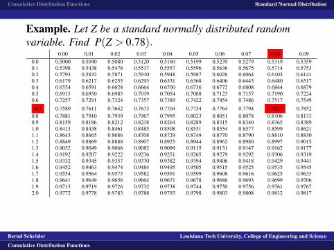
Cumulative Distribution Functions Standard Normal Distribution
Example. Let Z be a standard normally distributed randomvariable. Find P(Z > 0.78).
0.00 0.01 0.02 0.03 0.04 0.05 0.06 0.07 0.08 0.090.0 0.5000 0.5040 0.5080 0.5120 0.5160 0.5199 0.5239 0.5279 0.5319 0.53590.1 0.5398 0.5438 0.5478 0.5517 0.5557 0.5596 0.5636 0.5675 0.5714 0.57530.2 0.5793 0.5832 0.5871 0.5910 0.5948 0.5987 0.6026 0.6064 0.6103 0.61410.3 0.6179 0.6217 0.6255 0.6293 0.6331 0.6368 0.6406 0.6443 0.6480 0.65170.4 0.6554 0.6591 0.6628 0.6664 0.6700 0.6736 0.6772 0.6808 0.6844 0.68790.5 0.6915 0.6950 0.6985 0.7019 0.7054 0.7088 0.7123 0.7157 0.7190 0.72240.6 0.7257 0.7291 0.7324 0.7357 0.7389 0.7422 0.7454 0.7486 0.7517 0.7549
0.7 0.7580 0.7611 0.7642 0.7673 0.7704 0.7734 0.7764 0.7794 0.7823 0.78520.8 0.7881 0.7910 0.7939 0.7967 0.7995 0.8023 0.8051 0.8078 0.8106 0.81330.9 0.8159 0.8186 0.8212 0.8238 0.8264 0.8289 0.8315 0.8340 0.8365 0.83891.0 0.8413 0.8438 0.8461 0.8485 0.8508 0.8531 0.8554 0.8577 0.8599 0.86211.1 0.8643 0.8665 0.8686 0.8708 0.8729 0.8749 0.8770 0.8790 0.8810 0.88301.2 0.8849 0.8869 0.8888 0.8907 0.8925 0.8944 0.8962 0.8980 0.8997 0.90151.3 0.9032 0.9049 0.9066 0.9082 0.9099 0.9115 0.9131 0.9147 0.9162 0.91771.4 0.9192 0.9207 0.9222 0.9236 0.9251 0.9265 0.9279 0.9292 0.9306 0.93191.5 0.9332 0.9345 0.9357 0.9370 0.9382 0.9394 0.9406 0.9418 0.9429 0.94411.6 0.9452 0.9463 0.9474 0.9484 0.9495 0.9505 0.9515 0.9525 0.9535 0.95451.7 0.9554 0.9564 0.9573 0.9582 0.9591 0.9599 0.9608 0.9616 0.9625 0.96331.8 0.9641 0.9649 0.9656 0.9664 0.9671 0.9678 0.9686 0.9693 0.9699 0.97061.9 0.9713 0.9719 0.9726 0.9732 0.9738 0.9744 0.9750 0.9756 0.9761 0.97672.0 0.9772 0.9778 0.9783 0.9788 0.9793 0.9798 0.9803 0.9808 0.9812 0.9817
P(Z > 0.78) = 1−P(Z ≤ 0.78)≈ 1−0.7823 = 0.2177
Bernd Schroder Louisiana Tech University, College of Engineering and Science
Cumulative Distribution Functions
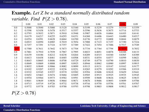
Cumulative Distribution Functions Standard Normal Distribution
Example. Let Z be a standard normally distributed randomvariable. Find P(Z > 0.78).
0.00 0.01 0.02 0.03 0.04 0.05 0.06 0.07 0.08 0.090.0 0.5000 0.5040 0.5080 0.5120 0.5160 0.5199 0.5239 0.5279 0.5319 0.53590.1 0.5398 0.5438 0.5478 0.5517 0.5557 0.5596 0.5636 0.5675 0.5714 0.57530.2 0.5793 0.5832 0.5871 0.5910 0.5948 0.5987 0.6026 0.6064 0.6103 0.61410.3 0.6179 0.6217 0.6255 0.6293 0.6331 0.6368 0.6406 0.6443 0.6480 0.65170.4 0.6554 0.6591 0.6628 0.6664 0.6700 0.6736 0.6772 0.6808 0.6844 0.68790.5 0.6915 0.6950 0.6985 0.7019 0.7054 0.7088 0.7123 0.7157 0.7190 0.72240.6 0.7257 0.7291 0.7324 0.7357 0.7389 0.7422 0.7454 0.7486 0.7517 0.7549
0.7 0.7580 0.7611 0.7642 0.7673 0.7704 0.7734 0.7764 0.7794 0.7823 0.78520.8 0.7881 0.7910 0.7939 0.7967 0.7995 0.8023 0.8051 0.8078 0.8106 0.81330.9 0.8159 0.8186 0.8212 0.8238 0.8264 0.8289 0.8315 0.8340 0.8365 0.83891.0 0.8413 0.8438 0.8461 0.8485 0.8508 0.8531 0.8554 0.8577 0.8599 0.86211.1 0.8643 0.8665 0.8686 0.8708 0.8729 0.8749 0.8770 0.8790 0.8810 0.88301.2 0.8849 0.8869 0.8888 0.8907 0.8925 0.8944 0.8962 0.8980 0.8997 0.90151.3 0.9032 0.9049 0.9066 0.9082 0.9099 0.9115 0.9131 0.9147 0.9162 0.91771.4 0.9192 0.9207 0.9222 0.9236 0.9251 0.9265 0.9279 0.9292 0.9306 0.93191.5 0.9332 0.9345 0.9357 0.9370 0.9382 0.9394 0.9406 0.9418 0.9429 0.94411.6 0.9452 0.9463 0.9474 0.9484 0.9495 0.9505 0.9515 0.9525 0.9535 0.95451.7 0.9554 0.9564 0.9573 0.9582 0.9591 0.9599 0.9608 0.9616 0.9625 0.96331.8 0.9641 0.9649 0.9656 0.9664 0.9671 0.9678 0.9686 0.9693 0.9699 0.97061.9 0.9713 0.9719 0.9726 0.9732 0.9738 0.9744 0.9750 0.9756 0.9761 0.97672.0 0.9772 0.9778 0.9783 0.9788 0.9793 0.9798 0.9803 0.9808 0.9812 0.9817
P(Z > 0.78)
= 1−P(Z ≤ 0.78)≈ 1−0.7823 = 0.2177
Bernd Schroder Louisiana Tech University, College of Engineering and Science
Cumulative Distribution Functions
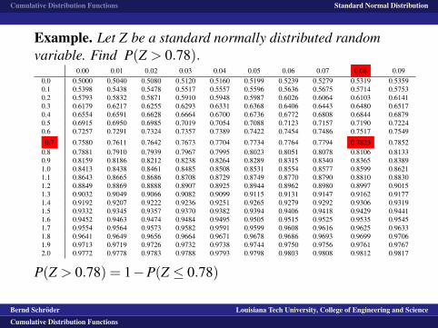
Cumulative Distribution Functions Standard Normal Distribution
Example. Let Z be a standard normally distributed randomvariable. Find P(Z > 0.78).
0.00 0.01 0.02 0.03 0.04 0.05 0.06 0.07 0.08 0.090.0 0.5000 0.5040 0.5080 0.5120 0.5160 0.5199 0.5239 0.5279 0.5319 0.53590.1 0.5398 0.5438 0.5478 0.5517 0.5557 0.5596 0.5636 0.5675 0.5714 0.57530.2 0.5793 0.5832 0.5871 0.5910 0.5948 0.5987 0.6026 0.6064 0.6103 0.61410.3 0.6179 0.6217 0.6255 0.6293 0.6331 0.6368 0.6406 0.6443 0.6480 0.65170.4 0.6554 0.6591 0.6628 0.6664 0.6700 0.6736 0.6772 0.6808 0.6844 0.68790.5 0.6915 0.6950 0.6985 0.7019 0.7054 0.7088 0.7123 0.7157 0.7190 0.72240.6 0.7257 0.7291 0.7324 0.7357 0.7389 0.7422 0.7454 0.7486 0.7517 0.7549
0.7 0.7580 0.7611 0.7642 0.7673 0.7704 0.7734 0.7764 0.7794 0.7823 0.78520.8 0.7881 0.7910 0.7939 0.7967 0.7995 0.8023 0.8051 0.8078 0.8106 0.81330.9 0.8159 0.8186 0.8212 0.8238 0.8264 0.8289 0.8315 0.8340 0.8365 0.83891.0 0.8413 0.8438 0.8461 0.8485 0.8508 0.8531 0.8554 0.8577 0.8599 0.86211.1 0.8643 0.8665 0.8686 0.8708 0.8729 0.8749 0.8770 0.8790 0.8810 0.88301.2 0.8849 0.8869 0.8888 0.8907 0.8925 0.8944 0.8962 0.8980 0.8997 0.90151.3 0.9032 0.9049 0.9066 0.9082 0.9099 0.9115 0.9131 0.9147 0.9162 0.91771.4 0.9192 0.9207 0.9222 0.9236 0.9251 0.9265 0.9279 0.9292 0.9306 0.93191.5 0.9332 0.9345 0.9357 0.9370 0.9382 0.9394 0.9406 0.9418 0.9429 0.94411.6 0.9452 0.9463 0.9474 0.9484 0.9495 0.9505 0.9515 0.9525 0.9535 0.95451.7 0.9554 0.9564 0.9573 0.9582 0.9591 0.9599 0.9608 0.9616 0.9625 0.96331.8 0.9641 0.9649 0.9656 0.9664 0.9671 0.9678 0.9686 0.9693 0.9699 0.97061.9 0.9713 0.9719 0.9726 0.9732 0.9738 0.9744 0.9750 0.9756 0.9761 0.97672.0 0.9772 0.9778 0.9783 0.9788 0.9793 0.9798 0.9803 0.9808 0.9812 0.9817
P(Z > 0.78) = 1−P(Z ≤ 0.78)
≈ 1−0.7823 = 0.2177
Bernd Schroder Louisiana Tech University, College of Engineering and Science
Cumulative Distribution Functions
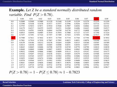
Cumulative Distribution Functions Standard Normal Distribution
Example. Let Z be a standard normally distributed randomvariable. Find P(Z > 0.78).
0.00 0.01 0.02 0.03 0.04 0.05 0.06 0.07 0.08 0.090.0 0.5000 0.5040 0.5080 0.5120 0.5160 0.5199 0.5239 0.5279 0.5319 0.53590.1 0.5398 0.5438 0.5478 0.5517 0.5557 0.5596 0.5636 0.5675 0.5714 0.57530.2 0.5793 0.5832 0.5871 0.5910 0.5948 0.5987 0.6026 0.6064 0.6103 0.61410.3 0.6179 0.6217 0.6255 0.6293 0.6331 0.6368 0.6406 0.6443 0.6480 0.65170.4 0.6554 0.6591 0.6628 0.6664 0.6700 0.6736 0.6772 0.6808 0.6844 0.68790.5 0.6915 0.6950 0.6985 0.7019 0.7054 0.7088 0.7123 0.7157 0.7190 0.72240.6 0.7257 0.7291 0.7324 0.7357 0.7389 0.7422 0.7454 0.7486 0.7517 0.7549
0.7 0.7580 0.7611 0.7642 0.7673 0.7704 0.7734 0.7764 0.7794 0.7823 0.78520.8 0.7881 0.7910 0.7939 0.7967 0.7995 0.8023 0.8051 0.8078 0.8106 0.81330.9 0.8159 0.8186 0.8212 0.8238 0.8264 0.8289 0.8315 0.8340 0.8365 0.83891.0 0.8413 0.8438 0.8461 0.8485 0.8508 0.8531 0.8554 0.8577 0.8599 0.86211.1 0.8643 0.8665 0.8686 0.8708 0.8729 0.8749 0.8770 0.8790 0.8810 0.88301.2 0.8849 0.8869 0.8888 0.8907 0.8925 0.8944 0.8962 0.8980 0.8997 0.90151.3 0.9032 0.9049 0.9066 0.9082 0.9099 0.9115 0.9131 0.9147 0.9162 0.91771.4 0.9192 0.9207 0.9222 0.9236 0.9251 0.9265 0.9279 0.9292 0.9306 0.93191.5 0.9332 0.9345 0.9357 0.9370 0.9382 0.9394 0.9406 0.9418 0.9429 0.94411.6 0.9452 0.9463 0.9474 0.9484 0.9495 0.9505 0.9515 0.9525 0.9535 0.95451.7 0.9554 0.9564 0.9573 0.9582 0.9591 0.9599 0.9608 0.9616 0.9625 0.96331.8 0.9641 0.9649 0.9656 0.9664 0.9671 0.9678 0.9686 0.9693 0.9699 0.97061.9 0.9713 0.9719 0.9726 0.9732 0.9738 0.9744 0.9750 0.9756 0.9761 0.97672.0 0.9772 0.9778 0.9783 0.9788 0.9793 0.9798 0.9803 0.9808 0.9812 0.9817
P(Z > 0.78) = 1−P(Z ≤ 0.78)≈ 1−0.7823
= 0.2177
Bernd Schroder Louisiana Tech University, College of Engineering and Science
Cumulative Distribution Functions
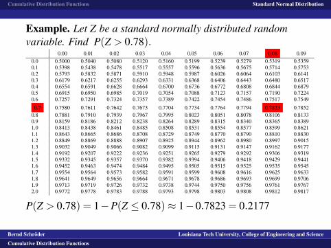
Cumulative Distribution Functions Standard Normal Distribution
Example. Let Z be a standard normally distributed randomvariable. Find P(Z > 0.78).
0.00 0.01 0.02 0.03 0.04 0.05 0.06 0.07 0.08 0.090.0 0.5000 0.5040 0.5080 0.5120 0.5160 0.5199 0.5239 0.5279 0.5319 0.53590.1 0.5398 0.5438 0.5478 0.5517 0.5557 0.5596 0.5636 0.5675 0.5714 0.57530.2 0.5793 0.5832 0.5871 0.5910 0.5948 0.5987 0.6026 0.6064 0.6103 0.61410.3 0.6179 0.6217 0.6255 0.6293 0.6331 0.6368 0.6406 0.6443 0.6480 0.65170.4 0.6554 0.6591 0.6628 0.6664 0.6700 0.6736 0.6772 0.6808 0.6844 0.68790.5 0.6915 0.6950 0.6985 0.7019 0.7054 0.7088 0.7123 0.7157 0.7190 0.72240.6 0.7257 0.7291 0.7324 0.7357 0.7389 0.7422 0.7454 0.7486 0.7517 0.7549
0.7 0.7580 0.7611 0.7642 0.7673 0.7704 0.7734 0.7764 0.7794 0.7823 0.78520.8 0.7881 0.7910 0.7939 0.7967 0.7995 0.8023 0.8051 0.8078 0.8106 0.81330.9 0.8159 0.8186 0.8212 0.8238 0.8264 0.8289 0.8315 0.8340 0.8365 0.83891.0 0.8413 0.8438 0.8461 0.8485 0.8508 0.8531 0.8554 0.8577 0.8599 0.86211.1 0.8643 0.8665 0.8686 0.8708 0.8729 0.8749 0.8770 0.8790 0.8810 0.88301.2 0.8849 0.8869 0.8888 0.8907 0.8925 0.8944 0.8962 0.8980 0.8997 0.90151.3 0.9032 0.9049 0.9066 0.9082 0.9099 0.9115 0.9131 0.9147 0.9162 0.91771.4 0.9192 0.9207 0.9222 0.9236 0.9251 0.9265 0.9279 0.9292 0.9306 0.93191.5 0.9332 0.9345 0.9357 0.9370 0.9382 0.9394 0.9406 0.9418 0.9429 0.94411.6 0.9452 0.9463 0.9474 0.9484 0.9495 0.9505 0.9515 0.9525 0.9535 0.95451.7 0.9554 0.9564 0.9573 0.9582 0.9591 0.9599 0.9608 0.9616 0.9625 0.96331.8 0.9641 0.9649 0.9656 0.9664 0.9671 0.9678 0.9686 0.9693 0.9699 0.97061.9 0.9713 0.9719 0.9726 0.9732 0.9738 0.9744 0.9750 0.9756 0.9761 0.97672.0 0.9772 0.9778 0.9783 0.9788 0.9793 0.9798 0.9803 0.9808 0.9812 0.9817
P(Z > 0.78) = 1−P(Z ≤ 0.78)≈ 1−0.7823 = 0.2177
Bernd Schroder Louisiana Tech University, College of Engineering and Science
Cumulative Distribution Functions
Cumulative Distribution Functions Standard Normal Distribution
Example. Let Z be a standard normally distributed randomvariable.
Find P(Z <−1.1).P(Z <−1.1) =
-z
6y
x
Bernd Schroder Louisiana Tech University, College of Engineering and Science
Cumulative Distribution Functions
Cumulative Distribution Functions Standard Normal Distribution
Example. Let Z be a standard normally distributed randomvariable. Find P(Z <−1.1).
P(Z <−1.1) =
-z
6y
x
Bernd Schroder Louisiana Tech University, College of Engineering and Science
Cumulative Distribution Functions
Cumulative Distribution Functions Standard Normal Distribution
Example. Let Z be a standard normally distributed randomvariable. Find P(Z <−1.1).P(Z <−1.1) =
-z
6y
x
Bernd Schroder Louisiana Tech University, College of Engineering and Science
Cumulative Distribution Functions

Cumulative Distribution Functions Standard Normal Distribution
Example. Let Z be a standard normally distributed randomvariable. Find P(Z <−1.1).P(Z <−1.1) =
-z
6y
x
Bernd Schroder Louisiana Tech University, College of Engineering and Science
Cumulative Distribution Functions

Cumulative Distribution Functions Standard Normal Distribution
Example. Let Z be a standard normally distributed randomvariable. Find P(Z <−1.1).P(Z <−1.1) =
-z
6y
x
Bernd Schroder Louisiana Tech University, College of Engineering and Science
Cumulative Distribution Functions
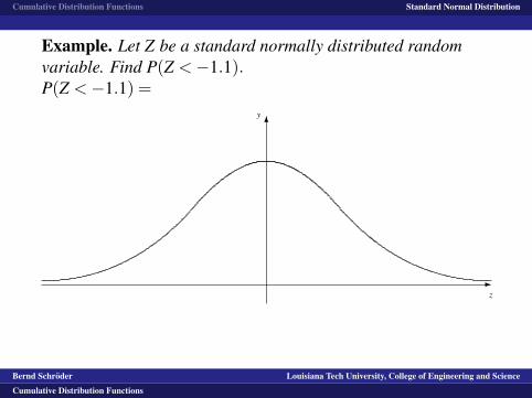
Cumulative Distribution Functions Standard Normal Distribution
Example. Let Z be a standard normally distributed randomvariable. Find P(Z <−1.1).P(Z <−1.1) =
-z
6y
x
Bernd Schroder Louisiana Tech University, College of Engineering and Science
Cumulative Distribution Functions
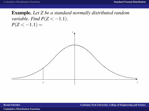
Cumulative Distribution Functions Standard Normal Distribution
Example. Let Z be a standard normally distributed randomvariable. Find P(Z <−1.1).P(Z <−1.1) =
-z
6y
x
Bernd Schroder Louisiana Tech University, College of Engineering and Science
Cumulative Distribution Functions

Cumulative Distribution Functions Standard Normal Distribution
Example. Let Z be a standard normally distributed randomvariable. Find P(Z <−1.1).P(Z <−1.1) =
-z
6y
x
Bernd Schroder Louisiana Tech University, College of Engineering and Science
Cumulative Distribution Functions
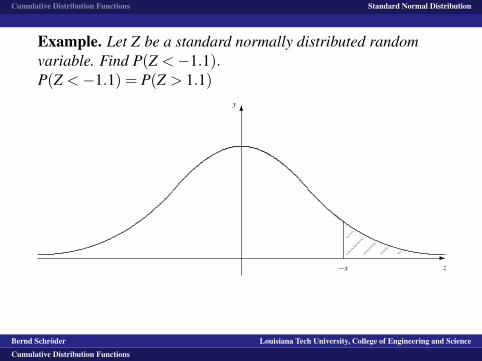
Cumulative Distribution Functions Standard Normal Distribution
Example. Let Z be a standard normally distributed randomvariable. Find P(Z <−1.1).P(Z <−1.1) = P(Z > 1.1)
-z
6y
−x
Bernd Schroder Louisiana Tech University, College of Engineering and Science
Cumulative Distribution Functions
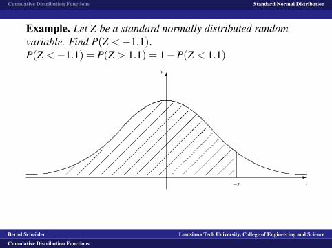
Cumulative Distribution Functions Standard Normal Distribution
Example. Let Z be a standard normally distributed randomvariable. Find P(Z <−1.1).P(Z <−1.1) = P(Z > 1.1) = 1−P(Z < 1.1)
-z
6y
−x
���
������
������
�������
��������
��������
��������
��������
���
Bernd Schroder Louisiana Tech University, College of Engineering and Science
Cumulative Distribution Functions
Cumulative Distribution Functions Standard Normal Distribution
Example. Let Z be a standard normally distributed randomvariable. Find P(Z <−1.1).P(Z <−1.1) = P(Z > 1.1) = 1−P(Z < 1.1)
0.00 0.01 0.02 0.03 0.04 0.05 0.06 0.07 0.08 0.090.0 0.5000 0.5040 0.5080 0.5120 0.5160 0.5199 0.5239 0.5279 0.5319 0.53590.1 0.5398 0.5438 0.5478 0.5517 0.5557 0.5596 0.5636 0.5675 0.5714 0.57530.2 0.5793 0.5832 0.5871 0.5910 0.5948 0.5987 0.6026 0.6064 0.6103 0.61410.3 0.6179 0.6217 0.6255 0.6293 0.6331 0.6368 0.6406 0.6443 0.6480 0.65170.4 0.6554 0.6591 0.6628 0.6664 0.6700 0.6736 0.6772 0.6808 0.6844 0.68790.5 0.6915 0.6950 0.6985 0.7019 0.7054 0.7088 0.7123 0.7157 0.7190 0.72240.6 0.7257 0.7291 0.7324 0.7357 0.7389 0.7422 0.7454 0.7486 0.7517 0.75490.7 0.7580 0.7611 0.7642 0.7673 0.7704 0.7734 0.7764 0.7794 0.7823 0.78520.8 0.7881 0.7910 0.7939 0.7967 0.7995 0.8023 0.8051 0.8078 0.8106 0.81330.9 0.8159 0.8186 0.8212 0.8238 0.8264 0.8289 0.8315 0.8340 0.8365 0.83891.0 0.8413 0.8438 0.8461 0.8485 0.8508 0.8531 0.8554 0.8577 0.8599 0.86211.1 0.8643 0.8665 0.8686 0.8708 0.8729 0.8749 0.8770 0.8790 0.8810 0.88301.2 0.8849 0.8869 0.8888 0.8907 0.8925 0.8944 0.8962 0.8980 0.8997 0.90151.3 0.9032 0.9049 0.9066 0.9082 0.9099 0.9115 0.9131 0.9147 0.9162 0.91771.4 0.9192 0.9207 0.9222 0.9236 0.9251 0.9265 0.9279 0.9292 0.9306 0.93191.5 0.9332 0.9345 0.9357 0.9370 0.9382 0.9394 0.9406 0.9418 0.9429 0.94411.6 0.9452 0.9463 0.9474 0.9484 0.9495 0.9505 0.9515 0.9525 0.9535 0.95451.7 0.9554 0.9564 0.9573 0.9582 0.9591 0.9599 0.9608 0.9616 0.9625 0.96331.8 0.9641 0.9649 0.9656 0.9664 0.9671 0.9678 0.9686 0.9693 0.9699 0.97061.9 0.9713 0.9719 0.9726 0.9732 0.9738 0.9744 0.9750 0.9756 0.9761 0.97672.0 0.9772 0.9778 0.9783 0.9788 0.9793 0.9798 0.9803 0.9808 0.9812 0.9817
P(Z <−1.1)≈ 1−0.8643 = 0.1357
Bernd Schroder Louisiana Tech University, College of Engineering and Science
Cumulative Distribution Functions
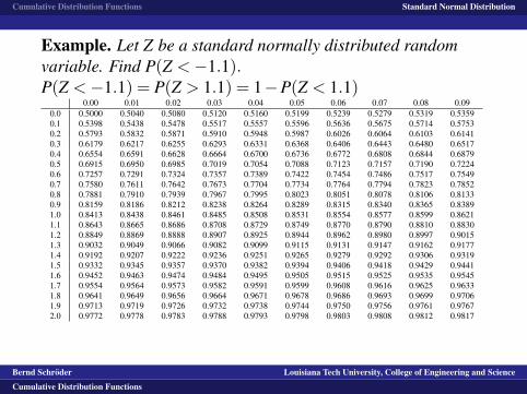
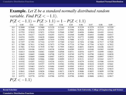
Cumulative Distribution Functions Standard Normal Distribution
Example. Let Z be a standard normally distributed randomvariable. Find P(Z <−1.1).P(Z <−1.1) = P(Z > 1.1) = 1−P(Z < 1.1)
0.00 0.01 0.02 0.03 0.04 0.05 0.06 0.07 0.08 0.090.0 0.5000 0.5040 0.5080 0.5120 0.5160 0.5199 0.5239 0.5279 0.5319 0.53590.1 0.5398 0.5438 0.5478 0.5517 0.5557 0.5596 0.5636 0.5675 0.5714 0.57530.2 0.5793 0.5832 0.5871 0.5910 0.5948 0.5987 0.6026 0.6064 0.6103 0.61410.3 0.6179 0.6217 0.6255 0.6293 0.6331 0.6368 0.6406 0.6443 0.6480 0.65170.4 0.6554 0.6591 0.6628 0.6664 0.6700 0.6736 0.6772 0.6808 0.6844 0.68790.5 0.6915 0.6950 0.6985 0.7019 0.7054 0.7088 0.7123 0.7157 0.7190 0.72240.6 0.7257 0.7291 0.7324 0.7357 0.7389 0.7422 0.7454 0.7486 0.7517 0.75490.7 0.7580 0.7611 0.7642 0.7673 0.7704 0.7734 0.7764 0.7794 0.7823 0.78520.8 0.7881 0.7910 0.7939 0.7967 0.7995 0.8023 0.8051 0.8078 0.8106 0.81330.9 0.8159 0.8186 0.8212 0.8238 0.8264 0.8289 0.8315 0.8340 0.8365 0.83891.0 0.8413 0.8438 0.8461 0.8485 0.8508 0.8531 0.8554 0.8577 0.8599 0.86211.1 0.8643 0.8665 0.8686 0.8708 0.8729 0.8749 0.8770 0.8790 0.8810 0.88301.2 0.8849 0.8869 0.8888 0.8907 0.8925 0.8944 0.8962 0.8980 0.8997 0.90151.3 0.9032 0.9049 0.9066 0.9082 0.9099 0.9115 0.9131 0.9147 0.9162 0.91771.4 0.9192 0.9207 0.9222 0.9236 0.9251 0.9265 0.9279 0.9292 0.9306 0.93191.5 0.9332 0.9345 0.9357 0.9370 0.9382 0.9394 0.9406 0.9418 0.9429 0.94411.6 0.9452 0.9463 0.9474 0.9484 0.9495 0.9505 0.9515 0.9525 0.9535 0.95451.7 0.9554 0.9564 0.9573 0.9582 0.9591 0.9599 0.9608 0.9616 0.9625 0.96331.8 0.9641 0.9649 0.9656 0.9664 0.9671 0.9678 0.9686 0.9693 0.9699 0.97061.9 0.9713 0.9719 0.9726 0.9732 0.9738 0.9744 0.9750 0.9756 0.9761 0.97672.0 0.9772 0.9778 0.9783 0.9788 0.9793 0.9798 0.9803 0.9808 0.9812 0.9817
P(Z <−1.1)
≈ 1−0.8643 = 0.1357
Bernd Schroder Louisiana Tech University, College of Engineering and Science
Cumulative Distribution Functions
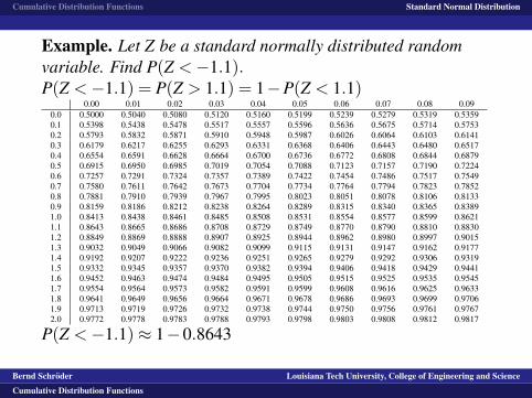
Cumulative Distribution Functions Standard Normal Distribution
Example. Let Z be a standard normally distributed randomvariable. Find P(Z <−1.1).P(Z <−1.1) = P(Z > 1.1) = 1−P(Z < 1.1)
0.00 0.01 0.02 0.03 0.04 0.05 0.06 0.07 0.08 0.090.0 0.5000 0.5040 0.5080 0.5120 0.5160 0.5199 0.5239 0.5279 0.5319 0.53590.1 0.5398 0.5438 0.5478 0.5517 0.5557 0.5596 0.5636 0.5675 0.5714 0.57530.2 0.5793 0.5832 0.5871 0.5910 0.5948 0.5987 0.6026 0.6064 0.6103 0.61410.3 0.6179 0.6217 0.6255 0.6293 0.6331 0.6368 0.6406 0.6443 0.6480 0.65170.4 0.6554 0.6591 0.6628 0.6664 0.6700 0.6736 0.6772 0.6808 0.6844 0.68790.5 0.6915 0.6950 0.6985 0.7019 0.7054 0.7088 0.7123 0.7157 0.7190 0.72240.6 0.7257 0.7291 0.7324 0.7357 0.7389 0.7422 0.7454 0.7486 0.7517 0.75490.7 0.7580 0.7611 0.7642 0.7673 0.7704 0.7734 0.7764 0.7794 0.7823 0.78520.8 0.7881 0.7910 0.7939 0.7967 0.7995 0.8023 0.8051 0.8078 0.8106 0.81330.9 0.8159 0.8186 0.8212 0.8238 0.8264 0.8289 0.8315 0.8340 0.8365 0.83891.0 0.8413 0.8438 0.8461 0.8485 0.8508 0.8531 0.8554 0.8577 0.8599 0.86211.1 0.8643 0.8665 0.8686 0.8708 0.8729 0.8749 0.8770 0.8790 0.8810 0.88301.2 0.8849 0.8869 0.8888 0.8907 0.8925 0.8944 0.8962 0.8980 0.8997 0.90151.3 0.9032 0.9049 0.9066 0.9082 0.9099 0.9115 0.9131 0.9147 0.9162 0.91771.4 0.9192 0.9207 0.9222 0.9236 0.9251 0.9265 0.9279 0.9292 0.9306 0.93191.5 0.9332 0.9345 0.9357 0.9370 0.9382 0.9394 0.9406 0.9418 0.9429 0.94411.6 0.9452 0.9463 0.9474 0.9484 0.9495 0.9505 0.9515 0.9525 0.9535 0.95451.7 0.9554 0.9564 0.9573 0.9582 0.9591 0.9599 0.9608 0.9616 0.9625 0.96331.8 0.9641 0.9649 0.9656 0.9664 0.9671 0.9678 0.9686 0.9693 0.9699 0.97061.9 0.9713 0.9719 0.9726 0.9732 0.9738 0.9744 0.9750 0.9756 0.9761 0.97672.0 0.9772 0.9778 0.9783 0.9788 0.9793 0.9798 0.9803 0.9808 0.9812 0.9817
P(Z <−1.1)≈ 1−0.8643
= 0.1357
Bernd Schroder Louisiana Tech University, College of Engineering and Science
Cumulative Distribution Functions
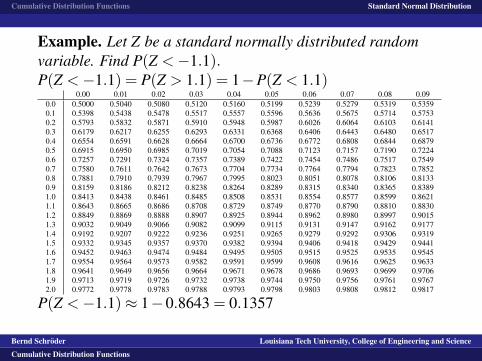
Cumulative Distribution Functions Standard Normal Distribution
Example. Let Z be a standard normally distributed randomvariable. Find P(Z <−1.1).P(Z <−1.1) = P(Z > 1.1) = 1−P(Z < 1.1)
0.00 0.01 0.02 0.03 0.04 0.05 0.06 0.07 0.08 0.090.0 0.5000 0.5040 0.5080 0.5120 0.5160 0.5199 0.5239 0.5279 0.5319 0.53590.1 0.5398 0.5438 0.5478 0.5517 0.5557 0.5596 0.5636 0.5675 0.5714 0.57530.2 0.5793 0.5832 0.5871 0.5910 0.5948 0.5987 0.6026 0.6064 0.6103 0.61410.3 0.6179 0.6217 0.6255 0.6293 0.6331 0.6368 0.6406 0.6443 0.6480 0.65170.4 0.6554 0.6591 0.6628 0.6664 0.6700 0.6736 0.6772 0.6808 0.6844 0.68790.5 0.6915 0.6950 0.6985 0.7019 0.7054 0.7088 0.7123 0.7157 0.7190 0.72240.6 0.7257 0.7291 0.7324 0.7357 0.7389 0.7422 0.7454 0.7486 0.7517 0.75490.7 0.7580 0.7611 0.7642 0.7673 0.7704 0.7734 0.7764 0.7794 0.7823 0.78520.8 0.7881 0.7910 0.7939 0.7967 0.7995 0.8023 0.8051 0.8078 0.8106 0.81330.9 0.8159 0.8186 0.8212 0.8238 0.8264 0.8289 0.8315 0.8340 0.8365 0.83891.0 0.8413 0.8438 0.8461 0.8485 0.8508 0.8531 0.8554 0.8577 0.8599 0.86211.1 0.8643 0.8665 0.8686 0.8708 0.8729 0.8749 0.8770 0.8790 0.8810 0.88301.2 0.8849 0.8869 0.8888 0.8907 0.8925 0.8944 0.8962 0.8980 0.8997 0.90151.3 0.9032 0.9049 0.9066 0.9082 0.9099 0.9115 0.9131 0.9147 0.9162 0.91771.4 0.9192 0.9207 0.9222 0.9236 0.9251 0.9265 0.9279 0.9292 0.9306 0.93191.5 0.9332 0.9345 0.9357 0.9370 0.9382 0.9394 0.9406 0.9418 0.9429 0.94411.6 0.9452 0.9463 0.9474 0.9484 0.9495 0.9505 0.9515 0.9525 0.9535 0.95451.7 0.9554 0.9564 0.9573 0.9582 0.9591 0.9599 0.9608 0.9616 0.9625 0.96331.8 0.9641 0.9649 0.9656 0.9664 0.9671 0.9678 0.9686 0.9693 0.9699 0.97061.9 0.9713 0.9719 0.9726 0.9732 0.9738 0.9744 0.9750 0.9756 0.9761 0.97672.0 0.9772 0.9778 0.9783 0.9788 0.9793 0.9798 0.9803 0.9808 0.9812 0.9817
P(Z <−1.1)≈ 1−0.8643 = 0.1357
Bernd Schroder Louisiana Tech University, College of Engineering and Science
Cumulative Distribution Functions

Cumulative Distribution Functions Standard Normal Distribution
Example. Let Z be a standard normally distributed randomvariable.
Find P(−0.5≤ Z ≤ 1.69).0.00 0.01 0.02 0.03 0.04 0.05 0.06 0.07 0.08 0.09
0.0 0.5000 0.5040 0.5080 0.5120 0.5160 0.5199 0.5239 0.5279 0.5319 0.53590.1 0.5398 0.5438 0.5478 0.5517 0.5557 0.5596 0.5636 0.5675 0.5714 0.57530.2 0.5793 0.5832 0.5871 0.5910 0.5948 0.5987 0.6026 0.6064 0.6103 0.61410.3 0.6179 0.6217 0.6255 0.6293 0.6331 0.6368 0.6406 0.6443 0.6480 0.65170.4 0.6554 0.6591 0.6628 0.6664 0.6700 0.6736 0.6772 0.6808 0.6844 0.68790.5 0.6915 0.6950 0.6985 0.7019 0.7054 0.7088 0.7123 0.7157 0.7190 0.72240.6 0.7257 0.7291 0.7324 0.7357 0.7389 0.7422 0.7454 0.7486 0.7517 0.75490.7 0.7580 0.7611 0.7642 0.7673 0.7704 0.7734 0.7764 0.7794 0.7823 0.78520.8 0.7881 0.7910 0.7939 0.7967 0.7995 0.8023 0.8051 0.8078 0.8106 0.81330.9 0.8159 0.8186 0.8212 0.8238 0.8264 0.8289 0.8315 0.8340 0.8365 0.83891.0 0.8413 0.8438 0.8461 0.8485 0.8508 0.8531 0.8554 0.8577 0.8599 0.86211.1 0.8643 0.8665 0.8686 0.8708 0.8729 0.8749 0.8770 0.8790 0.8810 0.88301.2 0.8849 0.8869 0.8888 0.8907 0.8925 0.8944 0.8962 0.8980 0.8997 0.90151.3 0.9032 0.9049 0.9066 0.9082 0.9099 0.9115 0.9131 0.9147 0.9162 0.91771.4 0.9192 0.9207 0.9222 0.9236 0.9251 0.9265 0.9279 0.9292 0.9306 0.93191.5 0.9332 0.9345 0.9357 0.9370 0.9382 0.9394 0.9406 0.9418 0.9429 0.94411.6 0.9452 0.9463 0.9474 0.9484 0.9495 0.9505 0.9515 0.9525 0.9535 0.95451.7 0.9554 0.9564 0.9573 0.9582 0.9591 0.9599 0.9608 0.9616 0.9625 0.9633
P(−0.5≤ Z ≤ 1.69)= P(Z ≤ 1.69)−P(Z ≤−0.5) = P(Z ≤ 1.69)−
(1−P(Z ≤ 0.5)
)= P(Z ≤ 1.69)+P(Z ≤ 0.5)−1≈ 0.9545+0.6915−1 = 0.6460
Bernd Schroder Louisiana Tech University, College of Engineering and Science
Cumulative Distribution Functions
Cumulative Distribution Functions Standard Normal Distribution
Example. Let Z be a standard normally distributed randomvariable. Find P(−0.5≤ Z ≤ 1.69).
0.00 0.01 0.02 0.03 0.04 0.05 0.06 0.07 0.08 0.090.0 0.5000 0.5040 0.5080 0.5120 0.5160 0.5199 0.5239 0.5279 0.5319 0.53590.1 0.5398 0.5438 0.5478 0.5517 0.5557 0.5596 0.5636 0.5675 0.5714 0.57530.2 0.5793 0.5832 0.5871 0.5910 0.5948 0.5987 0.6026 0.6064 0.6103 0.61410.3 0.6179 0.6217 0.6255 0.6293 0.6331 0.6368 0.6406 0.6443 0.6480 0.65170.4 0.6554 0.6591 0.6628 0.6664 0.6700 0.6736 0.6772 0.6808 0.6844 0.68790.5 0.6915 0.6950 0.6985 0.7019 0.7054 0.7088 0.7123 0.7157 0.7190 0.72240.6 0.7257 0.7291 0.7324 0.7357 0.7389 0.7422 0.7454 0.7486 0.7517 0.75490.7 0.7580 0.7611 0.7642 0.7673 0.7704 0.7734 0.7764 0.7794 0.7823 0.78520.8 0.7881 0.7910 0.7939 0.7967 0.7995 0.8023 0.8051 0.8078 0.8106 0.81330.9 0.8159 0.8186 0.8212 0.8238 0.8264 0.8289 0.8315 0.8340 0.8365 0.83891.0 0.8413 0.8438 0.8461 0.8485 0.8508 0.8531 0.8554 0.8577 0.8599 0.86211.1 0.8643 0.8665 0.8686 0.8708 0.8729 0.8749 0.8770 0.8790 0.8810 0.88301.2 0.8849 0.8869 0.8888 0.8907 0.8925 0.8944 0.8962 0.8980 0.8997 0.90151.3 0.9032 0.9049 0.9066 0.9082 0.9099 0.9115 0.9131 0.9147 0.9162 0.91771.4 0.9192 0.9207 0.9222 0.9236 0.9251 0.9265 0.9279 0.9292 0.9306 0.93191.5 0.9332 0.9345 0.9357 0.9370 0.9382 0.9394 0.9406 0.9418 0.9429 0.94411.6 0.9452 0.9463 0.9474 0.9484 0.9495 0.9505 0.9515 0.9525 0.9535 0.95451.7 0.9554 0.9564 0.9573 0.9582 0.9591 0.9599 0.9608 0.9616 0.9625 0.9633
P(−0.5≤ Z ≤ 1.69)= P(Z ≤ 1.69)−P(Z ≤−0.5) = P(Z ≤ 1.69)−
(1−P(Z ≤ 0.5)
)= P(Z ≤ 1.69)+P(Z ≤ 0.5)−1≈ 0.9545+0.6915−1 = 0.6460
Bernd Schroder Louisiana Tech University, College of Engineering and Science
Cumulative Distribution Functions
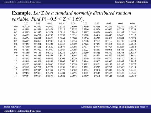
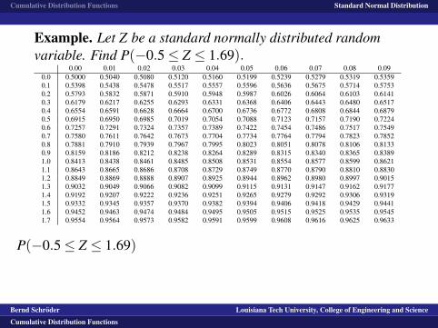
Cumulative Distribution Functions Standard Normal Distribution
Example. Let Z be a standard normally distributed randomvariable. Find P(−0.5≤ Z ≤ 1.69).
0.00 0.01 0.02 0.03 0.04 0.05 0.06 0.07 0.08 0.090.0 0.5000 0.5040 0.5080 0.5120 0.5160 0.5199 0.5239 0.5279 0.5319 0.53590.1 0.5398 0.5438 0.5478 0.5517 0.5557 0.5596 0.5636 0.5675 0.5714 0.57530.2 0.5793 0.5832 0.5871 0.5910 0.5948 0.5987 0.6026 0.6064 0.6103 0.61410.3 0.6179 0.6217 0.6255 0.6293 0.6331 0.6368 0.6406 0.6443 0.6480 0.65170.4 0.6554 0.6591 0.6628 0.6664 0.6700 0.6736 0.6772 0.6808 0.6844 0.68790.5 0.6915 0.6950 0.6985 0.7019 0.7054 0.7088 0.7123 0.7157 0.7190 0.72240.6 0.7257 0.7291 0.7324 0.7357 0.7389 0.7422 0.7454 0.7486 0.7517 0.75490.7 0.7580 0.7611 0.7642 0.7673 0.7704 0.7734 0.7764 0.7794 0.7823 0.78520.8 0.7881 0.7910 0.7939 0.7967 0.7995 0.8023 0.8051 0.8078 0.8106 0.81330.9 0.8159 0.8186 0.8212 0.8238 0.8264 0.8289 0.8315 0.8340 0.8365 0.83891.0 0.8413 0.8438 0.8461 0.8485 0.8508 0.8531 0.8554 0.8577 0.8599 0.86211.1 0.8643 0.8665 0.8686 0.8708 0.8729 0.8749 0.8770 0.8790 0.8810 0.88301.2 0.8849 0.8869 0.8888 0.8907 0.8925 0.8944 0.8962 0.8980 0.8997 0.90151.3 0.9032 0.9049 0.9066 0.9082 0.9099 0.9115 0.9131 0.9147 0.9162 0.91771.4 0.9192 0.9207 0.9222 0.9236 0.9251 0.9265 0.9279 0.9292 0.9306 0.93191.5 0.9332 0.9345 0.9357 0.9370 0.9382 0.9394 0.9406 0.9418 0.9429 0.94411.6 0.9452 0.9463 0.9474 0.9484 0.9495 0.9505 0.9515 0.9525 0.9535 0.95451.7 0.9554 0.9564 0.9573 0.9582 0.9591 0.9599 0.9608 0.9616 0.9625 0.9633
P(−0.5≤ Z ≤ 1.69)
= P(Z ≤ 1.69)−P(Z ≤−0.5) = P(Z ≤ 1.69)−(1−P(Z ≤ 0.5)
)= P(Z ≤ 1.69)+P(Z ≤ 0.5)−1≈ 0.9545+0.6915−1 = 0.6460
Bernd Schroder Louisiana Tech University, College of Engineering and Science
Cumulative Distribution Functions
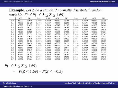
Cumulative Distribution Functions Standard Normal Distribution
Example. Let Z be a standard normally distributed randomvariable. Find P(−0.5≤ Z ≤ 1.69).
0.00 0.01 0.02 0.03 0.04 0.05 0.06 0.07 0.08 0.090.0 0.5000 0.5040 0.5080 0.5120 0.5160 0.5199 0.5239 0.5279 0.5319 0.53590.1 0.5398 0.5438 0.5478 0.5517 0.5557 0.5596 0.5636 0.5675 0.5714 0.57530.2 0.5793 0.5832 0.5871 0.5910 0.5948 0.5987 0.6026 0.6064 0.6103 0.61410.3 0.6179 0.6217 0.6255 0.6293 0.6331 0.6368 0.6406 0.6443 0.6480 0.65170.4 0.6554 0.6591 0.6628 0.6664 0.6700 0.6736 0.6772 0.6808 0.6844 0.68790.5 0.6915 0.6950 0.6985 0.7019 0.7054 0.7088 0.7123 0.7157 0.7190 0.72240.6 0.7257 0.7291 0.7324 0.7357 0.7389 0.7422 0.7454 0.7486 0.7517 0.75490.7 0.7580 0.7611 0.7642 0.7673 0.7704 0.7734 0.7764 0.7794 0.7823 0.78520.8 0.7881 0.7910 0.7939 0.7967 0.7995 0.8023 0.8051 0.8078 0.8106 0.81330.9 0.8159 0.8186 0.8212 0.8238 0.8264 0.8289 0.8315 0.8340 0.8365 0.83891.0 0.8413 0.8438 0.8461 0.8485 0.8508 0.8531 0.8554 0.8577 0.8599 0.86211.1 0.8643 0.8665 0.8686 0.8708 0.8729 0.8749 0.8770 0.8790 0.8810 0.88301.2 0.8849 0.8869 0.8888 0.8907 0.8925 0.8944 0.8962 0.8980 0.8997 0.90151.3 0.9032 0.9049 0.9066 0.9082 0.9099 0.9115 0.9131 0.9147 0.9162 0.91771.4 0.9192 0.9207 0.9222 0.9236 0.9251 0.9265 0.9279 0.9292 0.9306 0.93191.5 0.9332 0.9345 0.9357 0.9370 0.9382 0.9394 0.9406 0.9418 0.9429 0.94411.6 0.9452 0.9463 0.9474 0.9484 0.9495 0.9505 0.9515 0.9525 0.9535 0.95451.7 0.9554 0.9564 0.9573 0.9582 0.9591 0.9599 0.9608 0.9616 0.9625 0.9633
P(−0.5≤ Z ≤ 1.69)= P(Z ≤ 1.69)−P(Z ≤−0.5)
= P(Z ≤ 1.69)−(1−P(Z ≤ 0.5)
)= P(Z ≤ 1.69)+P(Z ≤ 0.5)−1≈ 0.9545+0.6915−1 = 0.6460
Bernd Schroder Louisiana Tech University, College of Engineering and Science
Cumulative Distribution Functions
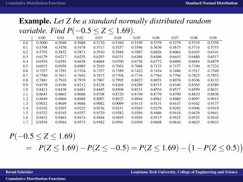
Cumulative Distribution Functions Standard Normal Distribution
Example. Let Z be a standard normally distributed randomvariable. Find P(−0.5≤ Z ≤ 1.69).
0.00 0.01 0.02 0.03 0.04 0.05 0.06 0.07 0.08 0.090.0 0.5000 0.5040 0.5080 0.5120 0.5160 0.5199 0.5239 0.5279 0.5319 0.53590.1 0.5398 0.5438 0.5478 0.5517 0.5557 0.5596 0.5636 0.5675 0.5714 0.57530.2 0.5793 0.5832 0.5871 0.5910 0.5948 0.5987 0.6026 0.6064 0.6103 0.61410.3 0.6179 0.6217 0.6255 0.6293 0.6331 0.6368 0.6406 0.6443 0.6480 0.65170.4 0.6554 0.6591 0.6628 0.6664 0.6700 0.6736 0.6772 0.6808 0.6844 0.68790.5 0.6915 0.6950 0.6985 0.7019 0.7054 0.7088 0.7123 0.7157 0.7190 0.72240.6 0.7257 0.7291 0.7324 0.7357 0.7389 0.7422 0.7454 0.7486 0.7517 0.75490.7 0.7580 0.7611 0.7642 0.7673 0.7704 0.7734 0.7764 0.7794 0.7823 0.78520.8 0.7881 0.7910 0.7939 0.7967 0.7995 0.8023 0.8051 0.8078 0.8106 0.81330.9 0.8159 0.8186 0.8212 0.8238 0.8264 0.8289 0.8315 0.8340 0.8365 0.83891.0 0.8413 0.8438 0.8461 0.8485 0.8508 0.8531 0.8554 0.8577 0.8599 0.86211.1 0.8643 0.8665 0.8686 0.8708 0.8729 0.8749 0.8770 0.8790 0.8810 0.88301.2 0.8849 0.8869 0.8888 0.8907 0.8925 0.8944 0.8962 0.8980 0.8997 0.90151.3 0.9032 0.9049 0.9066 0.9082 0.9099 0.9115 0.9131 0.9147 0.9162 0.91771.4 0.9192 0.9207 0.9222 0.9236 0.9251 0.9265 0.9279 0.9292 0.9306 0.93191.5 0.9332 0.9345 0.9357 0.9370 0.9382 0.9394 0.9406 0.9418 0.9429 0.94411.6 0.9452 0.9463 0.9474 0.9484 0.9495 0.9505 0.9515 0.9525 0.9535 0.95451.7 0.9554 0.9564 0.9573 0.9582 0.9591 0.9599 0.9608 0.9616 0.9625 0.9633
P(−0.5≤ Z ≤ 1.69)= P(Z ≤ 1.69)−P(Z ≤−0.5) = P(Z ≤ 1.69)−
(1−P(Z ≤ 0.5)
)
= P(Z ≤ 1.69)+P(Z ≤ 0.5)−1≈ 0.9545+0.6915−1 = 0.6460
Bernd Schroder Louisiana Tech University, College of Engineering and Science
Cumulative Distribution Functions
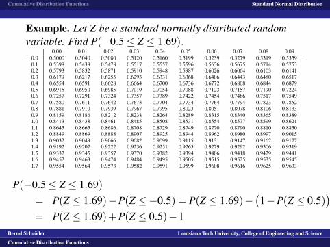
Cumulative Distribution Functions Standard Normal Distribution
Example. Let Z be a standard normally distributed randomvariable. Find P(−0.5≤ Z ≤ 1.69).
0.00 0.01 0.02 0.03 0.04 0.05 0.06 0.07 0.08 0.090.0 0.5000 0.5040 0.5080 0.5120 0.5160 0.5199 0.5239 0.5279 0.5319 0.53590.1 0.5398 0.5438 0.5478 0.5517 0.5557 0.5596 0.5636 0.5675 0.5714 0.57530.2 0.5793 0.5832 0.5871 0.5910 0.5948 0.5987 0.6026 0.6064 0.6103 0.61410.3 0.6179 0.6217 0.6255 0.6293 0.6331 0.6368 0.6406 0.6443 0.6480 0.65170.4 0.6554 0.6591 0.6628 0.6664 0.6700 0.6736 0.6772 0.6808 0.6844 0.68790.5 0.6915 0.6950 0.6985 0.7019 0.7054 0.7088 0.7123 0.7157 0.7190 0.72240.6 0.7257 0.7291 0.7324 0.7357 0.7389 0.7422 0.7454 0.7486 0.7517 0.75490.7 0.7580 0.7611 0.7642 0.7673 0.7704 0.7734 0.7764 0.7794 0.7823 0.78520.8 0.7881 0.7910 0.7939 0.7967 0.7995 0.8023 0.8051 0.8078 0.8106 0.81330.9 0.8159 0.8186 0.8212 0.8238 0.8264 0.8289 0.8315 0.8340 0.8365 0.83891.0 0.8413 0.8438 0.8461 0.8485 0.8508 0.8531 0.8554 0.8577 0.8599 0.86211.1 0.8643 0.8665 0.8686 0.8708 0.8729 0.8749 0.8770 0.8790 0.8810 0.88301.2 0.8849 0.8869 0.8888 0.8907 0.8925 0.8944 0.8962 0.8980 0.8997 0.90151.3 0.9032 0.9049 0.9066 0.9082 0.9099 0.9115 0.9131 0.9147 0.9162 0.91771.4 0.9192 0.9207 0.9222 0.9236 0.9251 0.9265 0.9279 0.9292 0.9306 0.93191.5 0.9332 0.9345 0.9357 0.9370 0.9382 0.9394 0.9406 0.9418 0.9429 0.94411.6 0.9452 0.9463 0.9474 0.9484 0.9495 0.9505 0.9515 0.9525 0.9535 0.95451.7 0.9554 0.9564 0.9573 0.9582 0.9591 0.9599 0.9608 0.9616 0.9625 0.9633
P(−0.5≤ Z ≤ 1.69)= P(Z ≤ 1.69)−P(Z ≤−0.5) = P(Z ≤ 1.69)−
(1−P(Z ≤ 0.5)
)= P(Z ≤ 1.69)+P(Z ≤ 0.5)−1
≈ 0.9545+0.6915−1 = 0.6460
Bernd Schroder Louisiana Tech University, College of Engineering and Science
Cumulative Distribution Functions

Cumulative Distribution Functions Standard Normal Distribution
Example. Let Z be a standard normally distributed randomvariable. Find P(−0.5≤ Z ≤ 1.69).
0.00 0.01 0.02 0.03 0.04 0.05 0.06 0.07 0.08 0.090.0 0.5000 0.5040 0.5080 0.5120 0.5160 0.5199 0.5239 0.5279 0.5319 0.53590.1 0.5398 0.5438 0.5478 0.5517 0.5557 0.5596 0.5636 0.5675 0.5714 0.57530.2 0.5793 0.5832 0.5871 0.5910 0.5948 0.5987 0.6026 0.6064 0.6103 0.61410.3 0.6179 0.6217 0.6255 0.6293 0.6331 0.6368 0.6406 0.6443 0.6480 0.65170.4 0.6554 0.6591 0.6628 0.6664 0.6700 0.6736 0.6772 0.6808 0.6844 0.68790.5 0.6915 0.6950 0.6985 0.7019 0.7054 0.7088 0.7123 0.7157 0.7190 0.72240.6 0.7257 0.7291 0.7324 0.7357 0.7389 0.7422 0.7454 0.7486 0.7517 0.75490.7 0.7580 0.7611 0.7642 0.7673 0.7704 0.7734 0.7764 0.7794 0.7823 0.78520.8 0.7881 0.7910 0.7939 0.7967 0.7995 0.8023 0.8051 0.8078 0.8106 0.81330.9 0.8159 0.8186 0.8212 0.8238 0.8264 0.8289 0.8315 0.8340 0.8365 0.83891.0 0.8413 0.8438 0.8461 0.8485 0.8508 0.8531 0.8554 0.8577 0.8599 0.86211.1 0.8643 0.8665 0.8686 0.8708 0.8729 0.8749 0.8770 0.8790 0.8810 0.88301.2 0.8849 0.8869 0.8888 0.8907 0.8925 0.8944 0.8962 0.8980 0.8997 0.90151.3 0.9032 0.9049 0.9066 0.9082 0.9099 0.9115 0.9131 0.9147 0.9162 0.91771.4 0.9192 0.9207 0.9222 0.9236 0.9251 0.9265 0.9279 0.9292 0.9306 0.93191.5 0.9332 0.9345 0.9357 0.9370 0.9382 0.9394 0.9406 0.9418 0.9429 0.94411.6 0.9452 0.9463 0.9474 0.9484 0.9495 0.9505 0.9515 0.9525 0.9535 0.95451.7 0.9554 0.9564 0.9573 0.9582 0.9591 0.9599 0.9608 0.9616 0.9625 0.9633
P(−0.5≤ Z ≤ 1.69)= P(Z ≤ 1.69)−P(Z ≤−0.5) = P(Z ≤ 1.69)−
(1−P(Z ≤ 0.5)
)= P(Z ≤ 1.69)+P(Z ≤ 0.5)−1≈ 0.9545
+0.6915−1 = 0.6460
Bernd Schroder Louisiana Tech University, College of Engineering and Science
Cumulative Distribution Functions

Cumulative Distribution Functions Standard Normal Distribution
Example. Let Z be a standard normally distributed randomvariable. Find P(−0.5≤ Z ≤ 1.69).
0.00 0.01 0.02 0.03 0.04 0.05 0.06 0.07 0.08 0.090.0 0.5000 0.5040 0.5080 0.5120 0.5160 0.5199 0.5239 0.5279 0.5319 0.53590.1 0.5398 0.5438 0.5478 0.5517 0.5557 0.5596 0.5636 0.5675 0.5714 0.57530.2 0.5793 0.5832 0.5871 0.5910 0.5948 0.5987 0.6026 0.6064 0.6103 0.61410.3 0.6179 0.6217 0.6255 0.6293 0.6331 0.6368 0.6406 0.6443 0.6480 0.65170.4 0.6554 0.6591 0.6628 0.6664 0.6700 0.6736 0.6772 0.6808 0.6844 0.68790.5 0.6915 0.6950 0.6985 0.7019 0.7054 0.7088 0.7123 0.7157 0.7190 0.72240.6 0.7257 0.7291 0.7324 0.7357 0.7389 0.7422 0.7454 0.7486 0.7517 0.75490.7 0.7580 0.7611 0.7642 0.7673 0.7704 0.7734 0.7764 0.7794 0.7823 0.78520.8 0.7881 0.7910 0.7939 0.7967 0.7995 0.8023 0.8051 0.8078 0.8106 0.81330.9 0.8159 0.8186 0.8212 0.8238 0.8264 0.8289 0.8315 0.8340 0.8365 0.83891.0 0.8413 0.8438 0.8461 0.8485 0.8508 0.8531 0.8554 0.8577 0.8599 0.86211.1 0.8643 0.8665 0.8686 0.8708 0.8729 0.8749 0.8770 0.8790 0.8810 0.88301.2 0.8849 0.8869 0.8888 0.8907 0.8925 0.8944 0.8962 0.8980 0.8997 0.90151.3 0.9032 0.9049 0.9066 0.9082 0.9099 0.9115 0.9131 0.9147 0.9162 0.91771.4 0.9192 0.9207 0.9222 0.9236 0.9251 0.9265 0.9279 0.9292 0.9306 0.93191.5 0.9332 0.9345 0.9357 0.9370 0.9382 0.9394 0.9406 0.9418 0.9429 0.94411.6 0.9452 0.9463 0.9474 0.9484 0.9495 0.9505 0.9515 0.9525 0.9535 0.95451.7 0.9554 0.9564 0.9573 0.9582 0.9591 0.9599 0.9608 0.9616 0.9625 0.9633
P(−0.5≤ Z ≤ 1.69)= P(Z ≤ 1.69)−P(Z ≤−0.5) = P(Z ≤ 1.69)−
(1−P(Z ≤ 0.5)
)= P(Z ≤ 1.69)+P(Z ≤ 0.5)−1≈ 0.9545+0.6915
−1 = 0.6460
Bernd Schroder Louisiana Tech University, College of Engineering and Science
Cumulative Distribution Functions
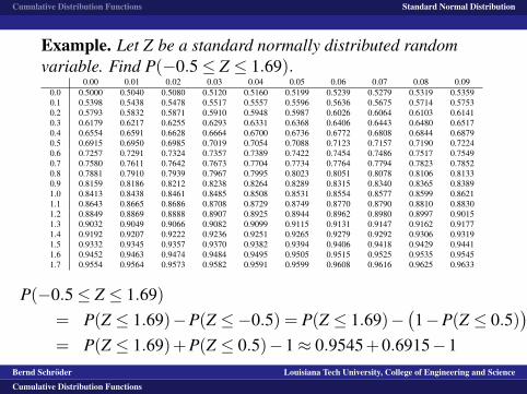
Cumulative Distribution Functions Standard Normal Distribution
Example. Let Z be a standard normally distributed randomvariable. Find P(−0.5≤ Z ≤ 1.69).
0.00 0.01 0.02 0.03 0.04 0.05 0.06 0.07 0.08 0.090.0 0.5000 0.5040 0.5080 0.5120 0.5160 0.5199 0.5239 0.5279 0.5319 0.53590.1 0.5398 0.5438 0.5478 0.5517 0.5557 0.5596 0.5636 0.5675 0.5714 0.57530.2 0.5793 0.5832 0.5871 0.5910 0.5948 0.5987 0.6026 0.6064 0.6103 0.61410.3 0.6179 0.6217 0.6255 0.6293 0.6331 0.6368 0.6406 0.6443 0.6480 0.65170.4 0.6554 0.6591 0.6628 0.6664 0.6700 0.6736 0.6772 0.6808 0.6844 0.68790.5 0.6915 0.6950 0.6985 0.7019 0.7054 0.7088 0.7123 0.7157 0.7190 0.72240.6 0.7257 0.7291 0.7324 0.7357 0.7389 0.7422 0.7454 0.7486 0.7517 0.75490.7 0.7580 0.7611 0.7642 0.7673 0.7704 0.7734 0.7764 0.7794 0.7823 0.78520.8 0.7881 0.7910 0.7939 0.7967 0.7995 0.8023 0.8051 0.8078 0.8106 0.81330.9 0.8159 0.8186 0.8212 0.8238 0.8264 0.8289 0.8315 0.8340 0.8365 0.83891.0 0.8413 0.8438 0.8461 0.8485 0.8508 0.8531 0.8554 0.8577 0.8599 0.86211.1 0.8643 0.8665 0.8686 0.8708 0.8729 0.8749 0.8770 0.8790 0.8810 0.88301.2 0.8849 0.8869 0.8888 0.8907 0.8925 0.8944 0.8962 0.8980 0.8997 0.90151.3 0.9032 0.9049 0.9066 0.9082 0.9099 0.9115 0.9131 0.9147 0.9162 0.91771.4 0.9192 0.9207 0.9222 0.9236 0.9251 0.9265 0.9279 0.9292 0.9306 0.93191.5 0.9332 0.9345 0.9357 0.9370 0.9382 0.9394 0.9406 0.9418 0.9429 0.94411.6 0.9452 0.9463 0.9474 0.9484 0.9495 0.9505 0.9515 0.9525 0.9535 0.95451.7 0.9554 0.9564 0.9573 0.9582 0.9591 0.9599 0.9608 0.9616 0.9625 0.9633
P(−0.5≤ Z ≤ 1.69)= P(Z ≤ 1.69)−P(Z ≤−0.5) = P(Z ≤ 1.69)−
(1−P(Z ≤ 0.5)
)= P(Z ≤ 1.69)+P(Z ≤ 0.5)−1≈ 0.9545+0.6915−1
= 0.6460
Bernd Schroder Louisiana Tech University, College of Engineering and Science
Cumulative Distribution Functions
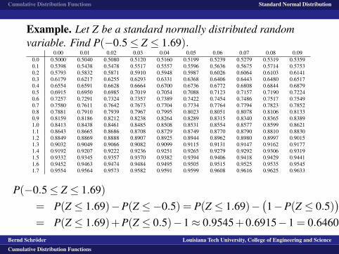
Cumulative Distribution Functions Standard Normal Distribution
Example. Let Z be a standard normally distributed randomvariable. Find P(−0.5≤ Z ≤ 1.69).
0.00 0.01 0.02 0.03 0.04 0.05 0.06 0.07 0.08 0.090.0 0.5000 0.5040 0.5080 0.5120 0.5160 0.5199 0.5239 0.5279 0.5319 0.53590.1 0.5398 0.5438 0.5478 0.5517 0.5557 0.5596 0.5636 0.5675 0.5714 0.57530.2 0.5793 0.5832 0.5871 0.5910 0.5948 0.5987 0.6026 0.6064 0.6103 0.61410.3 0.6179 0.6217 0.6255 0.6293 0.6331 0.6368 0.6406 0.6443 0.6480 0.65170.4 0.6554 0.6591 0.6628 0.6664 0.6700 0.6736 0.6772 0.6808 0.6844 0.68790.5 0.6915 0.6950 0.6985 0.7019 0.7054 0.7088 0.7123 0.7157 0.7190 0.72240.6 0.7257 0.7291 0.7324 0.7357 0.7389 0.7422 0.7454 0.7486 0.7517 0.75490.7 0.7580 0.7611 0.7642 0.7673 0.7704 0.7734 0.7764 0.7794 0.7823 0.78520.8 0.7881 0.7910 0.7939 0.7967 0.7995 0.8023 0.8051 0.8078 0.8106 0.81330.9 0.8159 0.8186 0.8212 0.8238 0.8264 0.8289 0.8315 0.8340 0.8365 0.83891.0 0.8413 0.8438 0.8461 0.8485 0.8508 0.8531 0.8554 0.8577 0.8599 0.86211.1 0.8643 0.8665 0.8686 0.8708 0.8729 0.8749 0.8770 0.8790 0.8810 0.88301.2 0.8849 0.8869 0.8888 0.8907 0.8925 0.8944 0.8962 0.8980 0.8997 0.90151.3 0.9032 0.9049 0.9066 0.9082 0.9099 0.9115 0.9131 0.9147 0.9162 0.91771.4 0.9192 0.9207 0.9222 0.9236 0.9251 0.9265 0.9279 0.9292 0.9306 0.93191.5 0.9332 0.9345 0.9357 0.9370 0.9382 0.9394 0.9406 0.9418 0.9429 0.94411.6 0.9452 0.9463 0.9474 0.9484 0.9495 0.9505 0.9515 0.9525 0.9535 0.95451.7 0.9554 0.9564 0.9573 0.9582 0.9591 0.9599 0.9608 0.9616 0.9625 0.9633
P(−0.5≤ Z ≤ 1.69)= P(Z ≤ 1.69)−P(Z ≤−0.5) = P(Z ≤ 1.69)−
(1−P(Z ≤ 0.5)
)= P(Z ≤ 1.69)+P(Z ≤ 0.5)−1≈ 0.9545+0.6915−1 = 0.6460
Bernd Schroder Louisiana Tech University, College of Engineering and Science
Cumulative Distribution Functions

Cumulative Distribution Functions Standard Normal Distribution
Example. Let Z be a standard normally distributed randomvariable.
Compute the 80th percentile.
-z
6y
���
������
������
�������
��������
��������
��������
��������
���
0.8
x
Bernd Schroder Louisiana Tech University, College of Engineering and Science
Cumulative Distribution Functions

Cumulative Distribution Functions Standard Normal Distribution
Example. Let Z be a standard normally distributed randomvariable. Compute the 80th percentile.
-z
6y
���
������
������
�������
��������
��������
��������
��������
���
0.8
x
Bernd Schroder Louisiana Tech University, College of Engineering and Science
Cumulative Distribution Functions
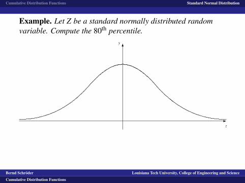
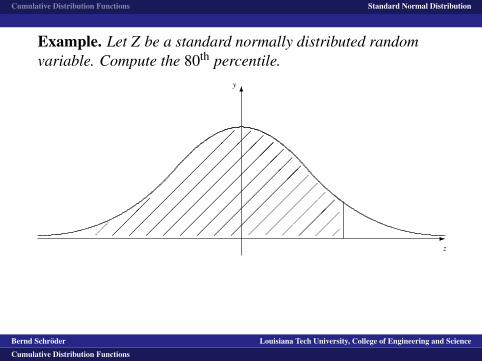
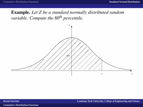

Cumulative Distribution Functions Standard Normal Distribution
Example. Let Z be a standard normally distributed randomvariable. Compute the 80th percentile.
η(80%)0.00 0.01 0.02 0.03 0.04 0.05 0.06 0.07 0.08 0.09
0.0 0.5000 0.5040 0.5080 0.5120 0.5160 0.5199 0.5239 0.5279 0.5319 0.53590.1 0.5398 0.5438 0.5478 0.5517 0.5557 0.5596 0.5636 0.5675 0.5714 0.57530.2 0.5793 0.5832 0.5871 0.5910 0.5948 0.5987 0.6026 0.6064 0.6103 0.61410.3 0.6179 0.6217 0.6255 0.6293 0.6331 0.6368 0.6406 0.6443 0.6480 0.65170.4 0.6554 0.6591 0.6628 0.6664 0.6700 0.6736 0.6772 0.6808 0.6844 0.68790.5 0.6915 0.6950 0.6985 0.7019 0.7054 0.7088 0.7123 0.7157 0.7190 0.72240.6 0.7257 0.7291 0.7324 0.7357 0.7389 0.7422 0.7454 0.7486 0.7517 0.75490.7 0.7580 0.7611 0.7642 0.7673 0.7704 0.7734 0.7764 0.7794 0.7823 0.78520.8 0.7881 0.7910 0.7939 0.7967 0.7995 0.8023 0.8051 0.8078 0.8106 0.81330.9 0.8159 0.8186 0.8212 0.8238 0.8264 0.8289 0.8315 0.8340 0.8365 0.83891.0 0.8413 0.8438 0.8461 0.8485 0.8508 0.8531 0.8554 0.8577 0.8599 0.86211.1 0.8643 0.8665 0.8686 0.8708 0.8729 0.8749 0.8770 0.8790 0.8810 0.88301.2 0.8849 0.8869 0.8888 0.8907 0.8925 0.8944 0.8962 0.8980 0.8997 0.90151.3 0.9032 0.9049 0.9066 0.9082 0.9099 0.9115 0.9131 0.9147 0.9162 0.91771.4 0.9192 0.9207 0.9222 0.9236 0.9251 0.9265 0.9279 0.9292 0.9306 0.93191.5 0.9332 0.9345 0.9357 0.9370 0.9382 0.9394 0.9406 0.9418 0.9429 0.94411.6 0.9452 0.9463 0.9474 0.9484 0.9495 0.9505 0.9515 0.9525 0.9535 0.95451.7 0.9554 0.9564 0.9573 0.9582 0.9591 0.9599 0.9608 0.9616 0.9625 0.96331.8 0.9641 0.9649 0.9656 0.9664 0.9671 0.9678 0.9686 0.9693 0.9699 0.97061.9 0.9713 0.9719 0.9726 0.9732 0.9738 0.9744 0.9750 0.9756 0.9761 0.97672.0 0.9772 0.9778 0.9783 0.9788 0.9793 0.9798 0.9803 0.9808 0.9812 0.9817
Bernd Schroder Louisiana Tech University, College of Engineering and Science
Cumulative Distribution Functions
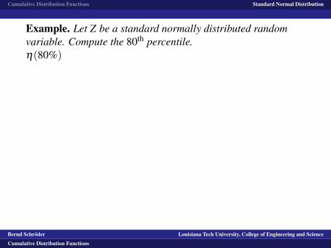
Cumulative Distribution Functions Standard Normal Distribution
Example. Let Z be a standard normally distributed randomvariable. Compute the 80th percentile.η(80%)
0.00 0.01 0.02 0.03 0.04 0.05 0.06 0.07 0.08 0.090.0 0.5000 0.5040 0.5080 0.5120 0.5160 0.5199 0.5239 0.5279 0.5319 0.53590.1 0.5398 0.5438 0.5478 0.5517 0.5557 0.5596 0.5636 0.5675 0.5714 0.57530.2 0.5793 0.5832 0.5871 0.5910 0.5948 0.5987 0.6026 0.6064 0.6103 0.61410.3 0.6179 0.6217 0.6255 0.6293 0.6331 0.6368 0.6406 0.6443 0.6480 0.65170.4 0.6554 0.6591 0.6628 0.6664 0.6700 0.6736 0.6772 0.6808 0.6844 0.68790.5 0.6915 0.6950 0.6985 0.7019 0.7054 0.7088 0.7123 0.7157 0.7190 0.72240.6 0.7257 0.7291 0.7324 0.7357 0.7389 0.7422 0.7454 0.7486 0.7517 0.75490.7 0.7580 0.7611 0.7642 0.7673 0.7704 0.7734 0.7764 0.7794 0.7823 0.78520.8 0.7881 0.7910 0.7939 0.7967 0.7995 0.8023 0.8051 0.8078 0.8106 0.81330.9 0.8159 0.8186 0.8212 0.8238 0.8264 0.8289 0.8315 0.8340 0.8365 0.83891.0 0.8413 0.8438 0.8461 0.8485 0.8508 0.8531 0.8554 0.8577 0.8599 0.86211.1 0.8643 0.8665 0.8686 0.8708 0.8729 0.8749 0.8770 0.8790 0.8810 0.88301.2 0.8849 0.8869 0.8888 0.8907 0.8925 0.8944 0.8962 0.8980 0.8997 0.90151.3 0.9032 0.9049 0.9066 0.9082 0.9099 0.9115 0.9131 0.9147 0.9162 0.91771.4 0.9192 0.9207 0.9222 0.9236 0.9251 0.9265 0.9279 0.9292 0.9306 0.93191.5 0.9332 0.9345 0.9357 0.9370 0.9382 0.9394 0.9406 0.9418 0.9429 0.94411.6 0.9452 0.9463 0.9474 0.9484 0.9495 0.9505 0.9515 0.9525 0.9535 0.95451.7 0.9554 0.9564 0.9573 0.9582 0.9591 0.9599 0.9608 0.9616 0.9625 0.96331.8 0.9641 0.9649 0.9656 0.9664 0.9671 0.9678 0.9686 0.9693 0.9699 0.97061.9 0.9713 0.9719 0.9726 0.9732 0.9738 0.9744 0.9750 0.9756 0.9761 0.97672.0 0.9772 0.9778 0.9783 0.9788 0.9793 0.9798 0.9803 0.9808 0.9812 0.9817
Bernd Schroder Louisiana Tech University, College of Engineering and Science
Cumulative Distribution Functions
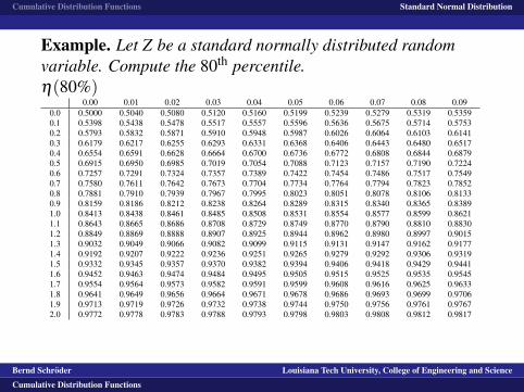
Cumulative Distribution Functions Standard Normal Distribution
Example. Let Z be a standard normally distributed randomvariable. Compute the 80th percentile.η(80%)
0.00 0.01 0.02 0.03 0.04 0.05 0.06 0.07 0.08 0.090.0 0.5000 0.5040 0.5080 0.5120 0.5160 0.5199 0.5239 0.5279 0.5319 0.53590.1 0.5398 0.5438 0.5478 0.5517 0.5557 0.5596 0.5636 0.5675 0.5714 0.57530.2 0.5793 0.5832 0.5871 0.5910 0.5948 0.5987 0.6026 0.6064 0.6103 0.61410.3 0.6179 0.6217 0.6255 0.6293 0.6331 0.6368 0.6406 0.6443 0.6480 0.65170.4 0.6554 0.6591 0.6628 0.6664 0.6700 0.6736 0.6772 0.6808 0.6844 0.68790.5 0.6915 0.6950 0.6985 0.7019 0.7054 0.7088 0.7123 0.7157 0.7190 0.72240.6 0.7257 0.7291 0.7324 0.7357 0.7389 0.7422 0.7454 0.7486 0.7517 0.75490.7 0.7580 0.7611 0.7642 0.7673 0.7704 0.7734 0.7764 0.7794 0.7823 0.78520.8 0.7881 0.7910 0.7939 0.7967 0.7995 0.8023 0.8051 0.8078 0.8106 0.81330.9 0.8159 0.8186 0.8212 0.8238 0.8264 0.8289 0.8315 0.8340 0.8365 0.83891.0 0.8413 0.8438 0.8461 0.8485 0.8508 0.8531 0.8554 0.8577 0.8599 0.86211.1 0.8643 0.8665 0.8686 0.8708 0.8729 0.8749 0.8770 0.8790 0.8810 0.88301.2 0.8849 0.8869 0.8888 0.8907 0.8925 0.8944 0.8962 0.8980 0.8997 0.90151.3 0.9032 0.9049 0.9066 0.9082 0.9099 0.9115 0.9131 0.9147 0.9162 0.91771.4 0.9192 0.9207 0.9222 0.9236 0.9251 0.9265 0.9279 0.9292 0.9306 0.93191.5 0.9332 0.9345 0.9357 0.9370 0.9382 0.9394 0.9406 0.9418 0.9429 0.94411.6 0.9452 0.9463 0.9474 0.9484 0.9495 0.9505 0.9515 0.9525 0.9535 0.95451.7 0.9554 0.9564 0.9573 0.9582 0.9591 0.9599 0.9608 0.9616 0.9625 0.96331.8 0.9641 0.9649 0.9656 0.9664 0.9671 0.9678 0.9686 0.9693 0.9699 0.97061.9 0.9713 0.9719 0.9726 0.9732 0.9738 0.9744 0.9750 0.9756 0.9761 0.97672.0 0.9772 0.9778 0.9783 0.9788 0.9793 0.9798 0.9803 0.9808 0.9812 0.9817
Bernd Schroder Louisiana Tech University, College of Engineering and Science
Cumulative Distribution Functions
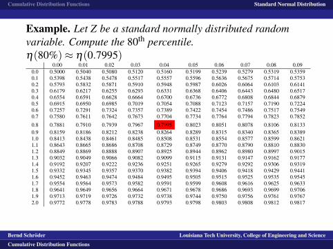
Cumulative Distribution Functions Standard Normal Distribution
Example. Let Z be a standard normally distributed randomvariable. Compute the 80th percentile.η(80%)≈ η(0.7995)
0.00 0.01 0.02 0.03 0.04 0.05 0.06 0.07 0.08 0.090.0 0.5000 0.5040 0.5080 0.5120 0.5160 0.5199 0.5239 0.5279 0.5319 0.53590.1 0.5398 0.5438 0.5478 0.5517 0.5557 0.5596 0.5636 0.5675 0.5714 0.57530.2 0.5793 0.5832 0.5871 0.5910 0.5948 0.5987 0.6026 0.6064 0.6103 0.61410.3 0.6179 0.6217 0.6255 0.6293 0.6331 0.6368 0.6406 0.6443 0.6480 0.65170.4 0.6554 0.6591 0.6628 0.6664 0.6700 0.6736 0.6772 0.6808 0.6844 0.68790.5 0.6915 0.6950 0.6985 0.7019 0.7054 0.7088 0.7123 0.7157 0.7190 0.72240.6 0.7257 0.7291 0.7324 0.7357 0.7389 0.7422 0.7454 0.7486 0.7517 0.75490.7 0.7580 0.7611 0.7642 0.7673 0.7704 0.7734 0.7764 0.7794 0.7823 0.7852
0.8 0.7881 0.7910 0.7939 0.7967 0.7995 0.8023 0.8051 0.8078 0.8106 0.81330.9 0.8159 0.8186 0.8212 0.8238 0.8264 0.8289 0.8315 0.8340 0.8365 0.83891.0 0.8413 0.8438 0.8461 0.8485 0.8508 0.8531 0.8554 0.8577 0.8599 0.86211.1 0.8643 0.8665 0.8686 0.8708 0.8729 0.8749 0.8770 0.8790 0.8810 0.88301.2 0.8849 0.8869 0.8888 0.8907 0.8925 0.8944 0.8962 0.8980 0.8997 0.90151.3 0.9032 0.9049 0.9066 0.9082 0.9099 0.9115 0.9131 0.9147 0.9162 0.91771.4 0.9192 0.9207 0.9222 0.9236 0.9251 0.9265 0.9279 0.9292 0.9306 0.93191.5 0.9332 0.9345 0.9357 0.9370 0.9382 0.9394 0.9406 0.9418 0.9429 0.94411.6 0.9452 0.9463 0.9474 0.9484 0.9495 0.9505 0.9515 0.9525 0.9535 0.95451.7 0.9554 0.9564 0.9573 0.9582 0.9591 0.9599 0.9608 0.9616 0.9625 0.96331.8 0.9641 0.9649 0.9656 0.9664 0.9671 0.9678 0.9686 0.9693 0.9699 0.97061.9 0.9713 0.9719 0.9726 0.9732 0.9738 0.9744 0.9750 0.9756 0.9761 0.97672.0 0.9772 0.9778 0.9783 0.9788 0.9793 0.9798 0.9803 0.9808 0.9812 0.9817
Bernd Schroder Louisiana Tech University, College of Engineering and Science
Cumulative Distribution Functions
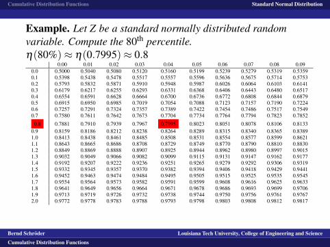
Cumulative Distribution Functions Standard Normal Distribution
Example. Let Z be a standard normally distributed randomvariable. Compute the 80th percentile.η(80%)≈ η(0.7995)≈ 0.8
0.00 0.01 0.02 0.03 0.04 0.05 0.06 0.07 0.08 0.090.0 0.5000 0.5040 0.5080 0.5120 0.5160 0.5199 0.5239 0.5279 0.5319 0.53590.1 0.5398 0.5438 0.5478 0.5517 0.5557 0.5596 0.5636 0.5675 0.5714 0.57530.2 0.5793 0.5832 0.5871 0.5910 0.5948 0.5987 0.6026 0.6064 0.6103 0.61410.3 0.6179 0.6217 0.6255 0.6293 0.6331 0.6368 0.6406 0.6443 0.6480 0.65170.4 0.6554 0.6591 0.6628 0.6664 0.6700 0.6736 0.6772 0.6808 0.6844 0.68790.5 0.6915 0.6950 0.6985 0.7019 0.7054 0.7088 0.7123 0.7157 0.7190 0.72240.6 0.7257 0.7291 0.7324 0.7357 0.7389 0.7422 0.7454 0.7486 0.7517 0.75490.7 0.7580 0.7611 0.7642 0.7673 0.7704 0.7734 0.7764 0.7794 0.7823 0.7852
0.8 0.7881 0.7910 0.7939 0.7967 0.7995 0.8023 0.8051 0.8078 0.8106 0.81330.9 0.8159 0.8186 0.8212 0.8238 0.8264 0.8289 0.8315 0.8340 0.8365 0.83891.0 0.8413 0.8438 0.8461 0.8485 0.8508 0.8531 0.8554 0.8577 0.8599 0.86211.1 0.8643 0.8665 0.8686 0.8708 0.8729 0.8749 0.8770 0.8790 0.8810 0.88301.2 0.8849 0.8869 0.8888 0.8907 0.8925 0.8944 0.8962 0.8980 0.8997 0.90151.3 0.9032 0.9049 0.9066 0.9082 0.9099 0.9115 0.9131 0.9147 0.9162 0.91771.4 0.9192 0.9207 0.9222 0.9236 0.9251 0.9265 0.9279 0.9292 0.9306 0.93191.5 0.9332 0.9345 0.9357 0.9370 0.9382 0.9394 0.9406 0.9418 0.9429 0.94411.6 0.9452 0.9463 0.9474 0.9484 0.9495 0.9505 0.9515 0.9525 0.9535 0.95451.7 0.9554 0.9564 0.9573 0.9582 0.9591 0.9599 0.9608 0.9616 0.9625 0.96331.8 0.9641 0.9649 0.9656 0.9664 0.9671 0.9678 0.9686 0.9693 0.9699 0.97061.9 0.9713 0.9719 0.9726 0.9732 0.9738 0.9744 0.9750 0.9756 0.9761 0.97672.0 0.9772 0.9778 0.9783 0.9788 0.9793 0.9798 0.9803 0.9808 0.9812 0.9817
Bernd Schroder Louisiana Tech University, College of Engineering and Science
Cumulative Distribution Functions
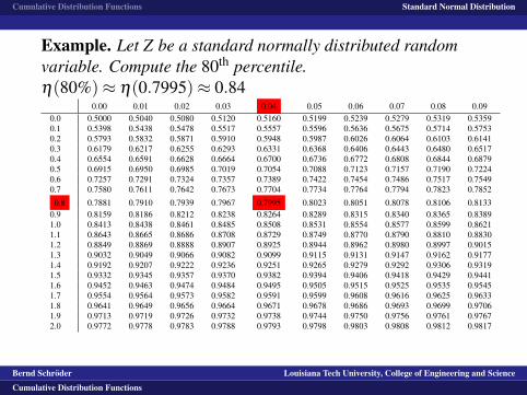
Cumulative Distribution Functions Standard Normal Distribution
Example. Let Z be a standard normally distributed randomvariable. Compute the 80th percentile.η(80%)≈ η(0.7995)≈ 0.84
0.00 0.01 0.02 0.03 0.04 0.05 0.06 0.07 0.08 0.090.0 0.5000 0.5040 0.5080 0.5120 0.5160 0.5199 0.5239 0.5279 0.5319 0.53590.1 0.5398 0.5438 0.5478 0.5517 0.5557 0.5596 0.5636 0.5675 0.5714 0.57530.2 0.5793 0.5832 0.5871 0.5910 0.5948 0.5987 0.6026 0.6064 0.6103 0.61410.3 0.6179 0.6217 0.6255 0.6293 0.6331 0.6368 0.6406 0.6443 0.6480 0.65170.4 0.6554 0.6591 0.6628 0.6664 0.6700 0.6736 0.6772 0.6808 0.6844 0.68790.5 0.6915 0.6950 0.6985 0.7019 0.7054 0.7088 0.7123 0.7157 0.7190 0.72240.6 0.7257 0.7291 0.7324 0.7357 0.7389 0.7422 0.7454 0.7486 0.7517 0.75490.7 0.7580 0.7611 0.7642 0.7673 0.7704 0.7734 0.7764 0.7794 0.7823 0.7852
0.8 0.7881 0.7910 0.7939 0.7967 0.7995 0.8023 0.8051 0.8078 0.8106 0.81330.9 0.8159 0.8186 0.8212 0.8238 0.8264 0.8289 0.8315 0.8340 0.8365 0.83891.0 0.8413 0.8438 0.8461 0.8485 0.8508 0.8531 0.8554 0.8577 0.8599 0.86211.1 0.8643 0.8665 0.8686 0.8708 0.8729 0.8749 0.8770 0.8790 0.8810 0.88301.2 0.8849 0.8869 0.8888 0.8907 0.8925 0.8944 0.8962 0.8980 0.8997 0.90151.3 0.9032 0.9049 0.9066 0.9082 0.9099 0.9115 0.9131 0.9147 0.9162 0.91771.4 0.9192 0.9207 0.9222 0.9236 0.9251 0.9265 0.9279 0.9292 0.9306 0.93191.5 0.9332 0.9345 0.9357 0.9370 0.9382 0.9394 0.9406 0.9418 0.9429 0.94411.6 0.9452 0.9463 0.9474 0.9484 0.9495 0.9505 0.9515 0.9525 0.9535 0.95451.7 0.9554 0.9564 0.9573 0.9582 0.9591 0.9599 0.9608 0.9616 0.9625 0.96331.8 0.9641 0.9649 0.9656 0.9664 0.9671 0.9678 0.9686 0.9693 0.9699 0.97061.9 0.9713 0.9719 0.9726 0.9732 0.9738 0.9744 0.9750 0.9756 0.9761 0.97672.0 0.9772 0.9778 0.9783 0.9788 0.9793 0.9798 0.9803 0.9808 0.9812 0.9817
Bernd Schroder Louisiana Tech University, College of Engineering and Science
Cumulative Distribution Functions