Embed Size (px)
Citation preview
N° D’ORDRE : 8445
UNIVERSITE PARIS-SUD XIFaculté des Sciences d’Orsay
THÈSE DE DOCTORAT
SPECIALITE : PHYSIQUE
Ecole Doctorale « Sciences et Technologies de l’Information des Télécommunications et des Systèmes »
Présentée par :
Ali Khaleghi
Sujet :
Diversity Antennas for Wireless LAN and Mobile Communication Handsets
« Etude d’antennes en Diversité pour Téléphone Mobiles et Réseaux
Locaux Radio électriques »
Soutenance le 18 Septembre 2006 devant le jury composé de :
M. A. Azoulay Professeur à Supelec de Gif-sur-Yvette Examinateur
M. J-C. Bolomey Professeur à l’Université Paris XI Directeur de thèse
M. P. Degauque Professeur à l’Université de Lile 1 Président
M. M. Drissi Professeur à l’Université de Rennes Rapporteur
M. P-S. Kildal Professeur à Chalmers University of Technology Rapporteur

i
Etude d’Antennes en Diversité pour Téléphones Mobiles
et Réseaux Locaux Radioélectriques
Khaleghi, A.
Résumé
Des niveaux élevés du rapport signal/bruit (SNR) sont nécessaires pour obtenir une
bonne qualité de service et de hauts débits pour les nouvelles générations de téléphones
mobiles (3G, 3,5 G) et pour les réseaux locaux sans fil (WiFi IEEE 802.11b/g/a). Afin
d’améliorer le SNR et de faire face aux effets de l'environnement (trajets multiples,
diffraction, brouillages) sur la transmission de données, il est possible d’appliquer aux
systèmes de radiocommunications, des techniques de diversité.
Cette thèse vise à approfondir les techniques de diversité appliquées aux mobiles de
radiotéléphonie et aux modules de réseaux locaux radioélectriques et à montrer les
possibilités d’amélioration de ces techniques en incluant plusieurs antennes dans le
système.
L’amélioration apportée par la diversité va dépendre très fortement des
caractéristiques des antennes utilisées et de l'environnement électromagnétique. Au
préalable, il est nécessaire de caractériser la propagation mobile : pour cela, différents
canaux mobiles de propagation sont étudiés et un simulateur de fading (trajets multiples)
est développé. Le simulateur de fading est combiné à une modélisation des angles
d’arrivée (AoA) afin de pouvoir calculer les performances des terminaux radio
incorporant de multiples antennes. La vérification de l’approche théorique est effectuée
grâce à des mesures réalisées dans la chambre réverbérante de Supelec. De plus, les
caractéristiques statistiques des signaux dus aux trajets multiples dans la chambre
réverbérante sont étudiées en détail.
En utilisant les méthodes proposées, les améliorations apportées par les techniques de
diversité d'antenne sont étudiés, en mettant l’accent sur le gain de diversité.
ii
La diversité d'antenne est étudiée dans un premier temps, pour deux antennes dipôles
parallèles en fonction de la distance de séparation de ces antennes, et validée ensuite par
les simulations et les mesures conduites dans la chambre réverbérante de Supelec. La
diversité de phase et du diagramme de rayonnement est identifiée et calculée pour des
antennes proches.
En fonction de ces résultats, un système simple et compact de diversité d'antenne de
téléphone mobile est réalisé. Ses performances prenant en compte le modèle humain de
fantôme (SAM) sont analysées à travers, entre autres, deux paramètres fondamentaux
dans ce type d’étude : le coefficient de corrélation des signaux incidents et le gain
efficace moyen de diversité (MEG).
Finalement, quatre systèmes compacts différents de diversité d'antenne ont été
conçus, simulés et réalisés pour des applications de réseaux locaux sans fil (WLAN).
Les antennes considérées ici utilisent la diversité de polarisation, de diagramme de
rayonnement et de phase en vue de l’amélioration de la qualité de réception du signal en
présence de trajets multiples. L’efficacité de la diversité est vérifiée par des simulations
électromagnétiques et par des mesures.
Abstract
iii
Diversity Antennas for Wireless LAN and Mobile
Communication Handsets
Khaleghi, A.
Abstract
High signal to noise ratio (SNR) levels are required to provide high data rate transmission
for the next generation of mobile and wireless devices. In order to provide high SNR and to
cope with the environmental impacts on the data transmission, diversity techniques are used.
This thesis investigates the performance enhancement that can be delivered by including
more antennas in the system.
The performance enhancement is dependent on the characteristics of the antennas and on
the wave propagation environment. Different mobile propagation channels are investigated
and a fading simulator is improved. The fading simulator is combined with the spherical
models for the field angle of arrivals to be able to calculate the performance of wireless
terminals with multiple antennas. The verification of the computations is performed by
measurements conducted in Supelec reverberation chamber. Furthermore, the statistical
characteristics of the multipath fading signals in the reverberation chamber are investigated
in detail.
Using the proposed methods, the antenna diversity performance enhancements in relation
to the relative displacement and orientation of the antennas and various spherical field
models are studied. Furthermore the gain improvements for the channels with correlated
signals and unbalanced powers are investigated.
Antenna diversity is studied for two parallel dipole antennas in relation to the separation
distance by the simulations and measurements in reverberation chamber. Radiation pattern
phase diversity is depicted for the coupled antennas. A simple and compact mobile phone
antenna diversity system is developed and the performance including phantom human head
model is investigated through mean effective gain, signals correlation coefficient and
diversity gain.

Abstract
iv
Four different and compact antenna diversity systems are designed, simulated and
manufactured for wireless LAN applications. The antennas make use of polarization, pattern
and phase diversities for signals reception in multipath channels. The performance
enhancement of the antenna systems are explored by the simulations and the measurements.
Table of Contents
viii
Table of Contents Chapter 1 Introduction .................................................................................................. 1
1.1 Objectives for this Thesis ................................................................................. 2 1.2 Organization of the Thesis................................................................................ 4
Chapter 2 Multipath Fading Characterization............................................................... 6 2.1 Introduction ...................................................................................................... 6 2.2 Characterization of Mobile Radio Propagation................................................ 6 2.3 The Nature of Multipath Propagation............................................................... 8 2.4 The Challenge of Communication over Fading Channels................................ 9 2.5 Short-term Fading........................................................................................... 11 2.6 Fading Models ................................................................................................ 12
2.6.1 Rayleigh fading model............................................................................ 14 2.6.2 Rician fading model ............................................................................... 15
2.7 Fading Simulator ............................................................................................ 15 2.8 Fading Simulator Models ............................................................................... 16 2.9 Empirical and Mathematical AoA Models..................................................... 20 2.10 Cross Polarization Power Ratio (XPR) .......................................................... 28 2.11 Mean Effective Gain (MEG) .......................................................................... 30
2.11.1 MEG measurements ............................................................................... 32 2.12 Summary......................................................................................................... 34
Chapter 3 Fading Simulator, Field Simulator and Reverberation Chamber ............... 36 3.1 Introduction .................................................................................................... 36 3.2 New Improved Fading Simulator ................................................................... 37 3.3 Field Simulator ............................................................................................... 42 3.4 New Improved Field Simulator ...................................................................... 45 3.5 Random Field Measurements ......................................................................... 47 3.6 Reverberation Chamber Enclosure................................................................. 50
3.6.1 Test frequency range .............................................................................. 52 3.6.2 Antennas ................................................................................................. 54 3.6.3 Working volume..................................................................................... 54 3.6.4 Mode modification techniques ............................................................... 54
3.7 MSRC Excitation and Signal Acquisition ...................................................... 56 3.8 Statistical Characterization ............................................................................. 61 3.9 Statistical Characteristics of Supelec MSRC ................................................. 63 3.10 Cross Polarization Ratio ................................................................................. 72 3.11 Field Periodicity Test ..................................................................................... 73 3.12 MEG and Antenna Efficiency Evaluation inside MSRC ............................... 75 3.13 Summary......................................................................................................... 76
Chapter 4 Multipath Fading Mitigation and Antenna Diversity ................................. 78 4.1 Introduction .................................................................................................... 78 4.2 Diversity Reception ........................................................................................ 79 4.3 Diversity Methods .......................................................................................... 80
4.3.1 Selection combining ............................................................................... 82
Table of Contents
ix
4.3.2 Maximum ratio combining ..................................................................... 84 4.3.3 Equal-gain combining ............................................................................ 85
4.4 Improvements from Diversity ........................................................................ 85 4.4.1 Level Crossing Rate and Average Fade Duration .................................. 90
4.5 Diversity and Signals Correlation Coefficient................................................ 92 4.5.1 Correlation coefficient: mutual impedance ............................................ 93 4.5.2 Correlation coefficient: radiation pattern ............................................... 94 4.5.3 Correlation coefficient: signals............................................................... 95
4.6 Correlation Coefficient for Space Diversity Antennas: Pattern Approach..... 96 4.7 Correlation Coefficient for Space Diversity Antennas: Signal Analysis ..... 100 4.8 Diversity Gain for Space Diversity Antennas: Signal Analysis ................... 103 4.9 Diversity Gain for Correlated Signals: Numerical Results .......................... 106 4.10 Diversity Gain for Correlated Signals and Imbalance Branches.................. 108 4.11 Diversity Evaluation from Measured Signals............................................... 110 4.12 Reverberation Chamber Measurements........................................................ 111
4.12.1 Spatial correlation coefficient for reverberation chamber.................... 111 4.12.2 LCR and AFD inside reverberation chamber ....................................... 116
4.13 Summery....................................................................................................... 117 Chapter 5 Antenna Diversity for Mobile Phone Communication............................. 119
5.1 Introduction .................................................................................................. 119 5.2 Diversity Techniques with Parallel Dipole Antennas: Pattern Analysis ...... 120
5.2.1 Signals Correlation coefficient: radiation pattern................................. 122 5.2.2 Measurement setup............................................................................... 129 5.2.3 Diversity gain ....................................................................................... 132 5.2.4 Antenna efficiency................................................................................ 134 5.2.5 Diversity gain versus separation distance: simulation.......................... 135
5.3 Antenna Diversity With Parasitic Elements ................................................. 136 5.4 Compact and Dual Band Antenna Diversity for Mobile Phones ................. 139
5.4.1 Antenna prototype ................................................................................ 140 5.4.2 Antenna simulation and measurement.................................................. 141 5.4.3 Farfield radiation pattern ...................................................................... 143 5.4.4 Signals correlation coefficient: mutual impedance .............................. 146 5.4.5 Signals correlation coefficient for GSM band: pattern approach ......... 146 5.4.6 Diversity gain using field simulator for GSM band ............................. 148 5.4.7 Antenna diversity performance for DCS band ..................................... 151 5.4.8 Antenna diversity measurement for GSM and DCS bands .................. 152 5.4.9 Antenna measurement using head model: GSM and DCS bands ........ 155 5.4.10 Correlation coefficient and diversity techniques .................................. 158 5.4.11 Local correlation coefficient................................................................. 159
5.5 Summery....................................................................................................... 161 Chapter 6 Polarization, Pattern and Phase Diversity Antennas for Wireless LAN Applications.................................................................................................................. 163
6.1 Introduction .................................................................................................. 163 6.2 Polarization Diversity Antenna for WLANs ................................................ 164
6.2.1 Antenna configuration and modeling ................................................... 165
Table of Contents
x
6.2.2 Theoretical Analysis ............................................................................. 166 6.2.3 Antenna simulation and measurements ................................................ 166 6.2.4 Radiation pattern................................................................................... 167 6.2.5 Antenna diversity evaluation................................................................ 168 6.2.6 Far-field pattern analysis of circular patch polarization diversity antenna 171 6.2.7 Conclusion............................................................................................ 176
6.3 Pattern Diversity Antennas Using Parasitic Switching Elements ................ 177 6.3.1 Preliminary research............................................................................. 179 6.3.2 Main radiator antenna design ............................................................... 182 6.3.3 Antenna simulation and measurement.................................................. 186 6.3.4 Diversity performance simulation ........................................................ 188 6.3.5 Diversity performance measurement.................................................... 190 6.3.6 Conclusion............................................................................................ 191
6.4 Integrated Diversity Antenna for WLANs ................................................... 191 6.4.1 Preliminary ........................................................................................... 192 6.4.2 Antenna design ..................................................................................... 193 6.4.3 Antenna simulation and optimization................................................... 194 6.4.4 Farfield radiation pattern ...................................................................... 196 6.4.5 Diversity antenna parameters evaluation.............................................. 198 6.4.6 Mean signal power ............................................................................... 203 6.4.7 Radiation pattern analysis and diversity techniques............................. 203 6.4.8 Conclusion............................................................................................ 203
6.5 A Compact and Broadband Diversity Antenna for WLANs........................ 204 6.5.1 Diversity antenna design ...................................................................... 205 6.5.2 Return loss and coupling ...................................................................... 206 6.5.3 Radiation pattern................................................................................... 207 6.5.4 Signals correlation coefficient .............................................................. 208 6.5.5 Signals measurement ............................................................................ 209 6.5.6 Radiation pattern analysis and diversity techniques............................. 211 6.5.7 Mean signal power ............................................................................... 211 6.5.8 Conclusion............................................................................................ 211
6.6 Diversity Gain Enhancement for WLAN antennas ...................................... 212 6.7 Summary....................................................................................................... 213
Conclusion…………………………………………………………………..………...215 References………………………………………………………………….…………218 Appendix I ……………………………………………………………………………224 Appendix II……………………………………………………………………………226 Appendix III…………………………………………………………………………..228
List of Figures
xi
List of Figures Figure 2-1 Typical mobile radio scenario illustrating multipath propagation in a terrestrial mobile radio environment [1]..................................................................................................7 Figure 2-2 Constructive and destructive addition of two transmission paths..........................8 Figure 2-3 How the envelope fades as two incoming signals combine with different phases 9 Figure 2-4 Typical behavior of the received signal in mobile communications [3]................9 Figure 2-5 Spatial frame of reference: φ is in the horizontal plane (xy- plane); θ is in the vertical plane .........................................................................................................................12 Figure 2-6 PDF of the Rayleigh distribution.........................................................................14 Figure 2-7 Comparison among autocorrelation of the simulated complex fading; Jakes model, improved Jakes model and Clarke reference model..................................................18 Figure 2-8 Comparison among autocorrelation of the simulated real-part fading; Jakes model, improved Jakes model and Clarke reference model..................................................19 Figure 2-9 Comparison among autocorrelation of the simulated imaginary-part fading; Jakes model, improved Jakes model and Clarke reference model ........................................19 Figure 2-10 Comparison among cross-correlation of the simulated fading signals; Jakes model, improved Jakes model and Clarke reference model (note that the reference model is always zero)...........................................................................................................................20 Figure 2-11 Spherical coordinate system and incident field representation..........................21 Figure 2-12 Form of the RF power spectrum using different scattering models: (___) Clarke’s model, (_ _ _) Aulin’s model, (- - -) improved Aulin model; θm=45° [3] .................22 Figure 2-13 Two truncated Gaussian functions corresponds to field elevation plane AoA distributions in urban environments ......................................................................................24 Figure 2-14 Illustration of the AoA distribution in various multipath propagation channels (a) Clarke model M1, uniform distribution in azimuth plane only (b) Taga model M2, Uniform distribution in azimuth and Gaussian distribution in the elevation (c) Kalliola model M3, Uniform azimuth and double exponential in elevation (d) Knudsen model M4, Gaussian distribution in elevation and elliptical distribution in azimuth; Red color show high dense scatters.................................................................................................................28 Figure 2-15 Mean effective gain of evaluated antennas, PIFA, MEMO, Discone in different multipath scattering field environments [25] ........................................................................32 Figure 2-16 Half wavelengths dipole antenna and its coordinate, α is the dipole inclination angle ......................................................................................................................................33 Figure 2-17 MEG of inclined half wavelengths dipole antenna in an environment with Gaussian distribution in elevation plane ( mv=mH=0° and σv=σH=30°) and uniform azimuth plane distribution [24] ...........................................................................................................33
List of Figures
xii
Figure 2-18 Distribution parameters giving constant MEG (-3dB) of dipole antennas regardless of the antenna orientation [24] .............................................................................34 Figure 3-1 Simulated fading signal power for N=50, β=0.2 .................................................39 Figure 3-2 Histogram of the simulated fading signals: real-part, imaginary-part and amplitude. Gaussian and Rayleigh PDF curves are also plotted for comparison..................39 Figure 3-3 Autocorrelation of the complex fading signals simulated for β=0.2; Clarke reference model is also plotted for comparison for fd supposed to be 0.1.............................40 Figure 3-4 Simulated Cross-correlation of the real and imaginary-part of fading for β=0.2 and the reference model.........................................................................................................40 Figure 3-5 Autocorrelation of the modeled fading signal for β=0.1, 0.2, 0.3, 0.4, 0.5 versus time lag ..................................................................................................................................41 Figure 3-6 Simulated cross-correlation of the fading signal for β=0.1, 0.2, 0.3, 0.4, 0.5 versus time lag.......................................................................................................................42 Figure 3-7 Indoor measurement setup for antenna performance evaluation in multipath environment using random field method...............................................................................49 Figure 3-8 Random field measurement using electromagnetic wave scatters.......................49 Figure 3-9 Random field measurement setup inside metallic shielded chamber ..................50 Figure 3-10 Supelec, large mode stirred reverberation chamber model................................52 Figure 3-11 Supelec large reverberation chamber photograph; The large metallic chamber, Network analyzer, and personal computer for controlling the rotating stirrer are illustrated...............................................................................................................................................53 Figure 3-12 Number of modes versus frequency (MHz) generated inside the Supelec MSRC....................................................................................................................................53 Figure 3-13 Rotating paddle model installed inside MSRC (Top) isometric and top view (bottom) the paddle photograph ............................................................................................55 Figure 3-14 Supelec mode stirred reverberation chamber model (top view), the placement of the rotating paddle and working zone are illustrated.............................................................56 Figure 3-15 Measurement setup for chamber statistical parameters evaluation including large reverberation , transmitting monopole antenna, receiving dipole antenna and network analyzer .................................................................................................................................58 Figure 3-16 Measured fading signal magnitude (normalized to mean) and phase inside MSRC for one revolution of the stirrer for 900, 1800, 2450 and 5100 MHz bands respectively; the receiving antenna installed inside the working volume of the chamber ...60 Figure 3-17 Normalized intensity moments (semi logarithmic scale) relevant to the amplitude of fading signal versus their order; (a) frequency 900MHz (b) frequency 1800MHz (c) frequency 2450MHz (d) frequency 5100MHz ...............................................63
List of Figures
xiii
Figure 3-18 Autocorrelation function of the measured signals versus samples shift (a) frequency: 900MHz (b) frequency: 1800MHz (c) frequency: 2450MHz (d) frequency: 5100MHz...............................................................................................................................64 Figure 3-19 Measured power samples normalized to mean with and without decimation; frequency: 900MHz, decimation rate: 1/25...........................................................................65 Figure 3-20 ACF of the measured signals at 900MHz after applying the decimation factor of 1/25 on the raw measured data..........................................................................................66 Figure 3-21 The histogram of the measured signals amplitude and the Rayleigh matched density functions(a) frequency: 900MHz (b) frequency: 1800MHz (c) frequency: 2450MHz (d) frequency: 5100MHz .......................................................................................................67 Figure 3-22 CDF plot of the measured signals amplitude and the reference Rayleigh distribution (constructed from a Rayleigh distributed population with the same parameter as the measured data) (a) frequency: 900MHz (b) frequency: 1800MHz (c) frequency: 2450MHz (d) frequency: 5100MHz......................................................................................68 Figure 3-23 Measured probability distribution function plot of the in-phase, quadrature and phase components of the fading signals for the test frequencies for 900,1800,2450 and 5100MHz...............................................................................................................................69 Figure 3-24 Measured and simulated autocorrelation of the fading signals for the complex, real and imaginary parts respectively (a)-(c). The cross-correlation of the fading is also illustrated in (d). The measurements are performed for 2450 MHz and the best matched results of the simulation is given for β=0.05 .........................................................................71 Figure 3-25 Uniformity of the average power distribution as a function of the stirrer positions at the operating frequencies for 900MHz, 1800MHz, 2450MHz and 5100MHz ..72 Figure 3-26 Measured PDF of the XPR (dB) for 2450MHz. The distribution is Gaussian with m= -0.23dB....................................................................................................................73 Figure 3-27 Measured signal power versus recording time for three revolution of the rotating paddle; frequency: 900MHz.....................................................................................74 Figure 3-28 Autocorrelation function of the measured signals versus time shift (sec) for three revolution of the rotating stirrer ...................................................................................74 Figure 4-1 correlation between the envelopes of signals received on two horizontally separated base station antennas as a function of the field arrival angle α. (___) α=5°, (_ _ _) α=10° ,(-----) α=20° ,(_._.) α=30°, (__ __) α=60°, (- - - -) α=90° [3]........................................80 Figure 4-2 Diversity reception systems: (a) selection (b) equal-gain (c) maximum ratio, combining..............................................................................................................................82 Figure 4-3 Cumulative distribution probability of output CNR (dB) for selection combining for various diversity orders (M) ............................................................................................83 Figure 4-4 Cumulative probability distribution of output CNR (dB) for maximum ratio combining (MRC) for various diversity orders ....................................................................84 Figure 4-5 CDF plot of the output CNR for two-branch diversity system for SC, MRC and EGC.......................................................................................................................................86
List of Figures
xiv
Figure 4-6 Diversity gain for maximum ratio combining and selection combining for two-branch diversity system for 0.1 and 0.01 CDF levels [50] ....................................................88 Figure 4-7 Diversity gain versus correlation coefficient and branches power imbalance for (a) SC, (b) EGC and (c) MRC based on equations given in (4-6).........................................89 Figure 4-8 LCR and AFD: LCR is the average number of positive-going crossing per second, AFD is the average of τ1, τ2, …, τn ...........................................................................90 Figure 4-9 Normalized LCR and AFD versus normalized signal level (dB) for two branch diversity system.....................................................................................................................91 Figure 4-10 Two vertically polarized radiating antennas representation in spherical coordinate system with distance d .........................................................................................97 Figure 4-11 Correlation coefficient between two vertically polarized isotropic antennas versus separation distance d(λ); AoAs are given by Taga model for mθ=0° and σθ values..98 Figure 4-12 Correlation coefficient between two vertically separated antennas with distance d; AoAs are given by Taga model for mθ=0° and σθ values..................................................99 Figure 4-13 Two horizontally spaced antennas in a multipath channel with Gaussian distributed field angle of arrivals with dispersion angle of σ and mθ ..................................100 Figure 4-14 Correlation coefficient versus spatial separation for two vertically polarized antennas; the incident field is considered, uniform in the azimuth plane and Gaussian in the elevation with σθ=1° and various mθ ...................................................................................100 Figure 4-15 Correlation coefficient between two isotropic radiating antennas versus separation distance. The antennas are exposed to scattering field with Clarke model for field AoA distribution..................................................................................................................101 Figure 4-16 Correlation coefficient between two isotropic radiating antennas versus separation distance. The antennas are exposed to scattering field with isotropic field AoA distribution...........................................................................................................................102 Figure 4-17 Correlation coefficient computation error versus number of uncorrelated signal samples ................................................................................................................................103 Figure 4-18 Computed received signal power using two isotropic antennas with separation distance of d=0.3λ and the signal variation rate for β=0.1 ..................................................103 Figure 4-19 CDF plot of the normalized signal powers (dB) in the diversity branches (P1 and P2) and after combining; the receiving antennas are isotropic and are separated with distance 0.3λ ........................................................................................................................104 Figure 4-20 Diversity gain versus separation distance for two isotropically radiating antennas and various signal combining techniques. The probability level α is 0.1.............105 Figure 4-21 Diversity gain versus separation distance (λ) for two isotropically radiating antennas and various signal combining techniques. The probability level α is 0.01...........105 Figure 4-22 Diversity gain (dB) versus correlation coefficient for α=0.01 and for selection, equal gain and maximum ratio combining. The best fitted curve is also illustrated for each case of combining................................................................................................................106
List of Figures
xv
Figure 4-23 Diversity gain (dB) versus correlation coefficient for α=0.1 and for selection, equal gain and maximum ratio combining. The best fitted curve is also illustrated for each case of combining................................................................................................................106 Figure 4-24 CDF plot of the simulated signals in diversity branches (P1) and after signals combining for various correlation coefficient. (a) selection combining (b) maximum ratio combining............................................................................................................................108 Figure 4-25 Diversity gain against correlation coefficient and power imbalance for α=0.1; (Left) SC and (Right) MRC...............................................................................................109 Figure 4-26 Diversity gain against correlation coefficient and power imbalance for α=0.01; (Left) SC and (Right) MRC.................................................................................................110 Figure 4-27 Measurement setup inside reverberation chamber for spatial correlation test.112 Figure 4-28 correlation coefficient between spatial points measured inside reverberation chamber; square envelop of the complex correlation, correlation between signals voltage and correlation between signals power are illustrated.........................................................114 Figure 4-29 Measured and computed correlation coefficient between two spatial points with distance d .............................................................................................................................115 Figure 4-30 Simulated spatial correlation coefficient versus distance in an isotropically scattering field channel. Two antenna types are used: isotropic radiation antenna and dipole antenna.................................................................................................................................116 Figure 4-31 Measured and theoretical normalized LCR versus normalized signal powers116 Figure 4-32 Measured and theoretical AFD versus normalized signal power ....................117 Figure 5-1 correlation coefficient as a function of antenna spacing: a comparison of Japanese workers’ experimental results [56].......................................................................120 Figure 5-2 Two parallel (half-wave) dipole antennas horizontally separated with distance d.............................................................................................................................................123 Figure 5-3 Envelop correlation coefficient between two half-wave dipoles with separation distance d; (---) computed from antenna element factor (___) Clarke’s function...............123 Figure 5-4 Simulated and measured mutual power coupling between two dipole antennas versus separation distance (λ)..............................................................................................124 Figure 5-5 Farfield radiation power pattern of two parallel dipole antennas for different separation distances for a) d=0.1λ, b) d=0.2λ and c) d=0.4λ and for each antenna port excitation when the other antenna is matched to 50Ω impedance.......................................125 Figure 5-6 Correlation coefficient as a function of antenna spacing (wavelengths), simulated and measured inside an isotropically scattered field environment. (---) Theory calculated; (…) overall simulated; (___) simulated using pattern-amplitude diversity effects; (-.-.-) simulated using pattern-phase diversity effects; (__o__) overall measured inside mode stirred reverberation chamber .........................................................................................................126 Figure 5-7 Simulated antenna prototype used for illustrating the pattern-phase diversity effects ..................................................................................................................................128
List of Figures
xvi
Figure 5-8 phase difference between radiation patterns versus spatial angles (θ, φ); a) The phase diversity generated, ∆Φ (Ω), between two coupled dipole antennas with separation distance d=0.1λ; b) an equivalent phase difference generated due to space diversity (βdcosφ sinθ) for d=0.2λ ...................................................................................................................129 Figure 5-9 Reverberation chamber measurement setup for two port signal acquisition .....130 Figure 5-10 Measured signal power at the diversity antenna ports for d=0.2λ ...................131 Figure 5-11 CDF of the measured signal powers inside MSRC for dipoles separation distance d=0.2λ: P1 and P2 are the measured signal powers in the diversity branches; PSC and PMRC are the signal powers after diversity combining: Sc and MRC, respectively; PSingle is the signal power received with a single antenna with no antenna close to it .....................133 Figure 5-12 Measured apparent diversity gain (dB) versus dipole separation (λ) for selection combining (SC) and maximum ratio combining (MRC) at 0.1 CDF level .........................133 Figure 5-13 Measured effective diversity gain (dB) versus dipole separation (λ) for selection combining (SC) and maximum ratio combining (MRC) at 0.1 CDF level .........................134 Figure 5-14 Simulated radiation efficiency degradation (dB) and measured mean signal power degradation (dB) in diversity configuration compared to single dipole antenna, versus separation distance (λ)..............................................................................................135 Figure 5-15 (a) simulated diversity gain versus dipoles distance for SC and MRC and α=0.1, α=0.01. (b) a sample CDF for d=0.2λ is illustrated.............................................................136 Figure 5-16 Single port pattern diversity antenna structure using two impedance loaded parasitic dipoles ...................................................................................................................137 Figure 5-17 Simulated radiation pattern of dipole diversity system for d=0.15λ, and a) Z1=∞, Z2=0 b) Z1=0, Z2=∞ ..................................................................................................138 Figure 5-18 Farfield radiation pattern of parasitic diversity configuration for Z1=-20j Ω (left) and Z’
1=-100j Ω (right)...............................................................................................139 Figure 5-19 (a) Sagem myc-2 mobile photograph (b) Antenna diversity prototype developed using two helical antennas...................................................................................................141 Figure 5-20 modeled handset diversity antenna and the Sagem helical antenna prototype.............................................................................................................................................141 Figure 5-21 Return loss and mutual power coupling (dB) for helical antennas versus frequency (MHz) (a) measured (b) Simulated model given in Figure 5-20........................143 Figure 5-22 Satimo spherical anechoic chamber test bed and the AUT position inside the chamber ...............................................................................................................................144 Figure 5-23 Left) simulated Right) measured farfield power gain (dBi) versus θ and φ spherical angles; antenna 1 is excited and antenna 2 is loaded by 50Ω impedance (see Figure 5-20). Frequency: 938MHz......................................................................................145 Figure 5-24 Left) simulated Right) measured farfield power gain (dBi) versus θ and φ spherical angles; antenna 1 is excited and antenna 2 is loaded by 50Ω impedance (see Figure 5-20); Frequency: 938MHz......................................................................................145
List of Figures
xvii
Figure 5-25 Simulated farfield patterns of the mobile diversity antennas in spherical coordinate system. The bolded line indicate 3dB beamwidth (GSM band)........................145 Figure 5-26 Computed envelop correlation coefficient in the GSM band based on the simulated and the measured radiation patterns....................................................................148 Figure 5-27 Diversity gain (dB) for different AoAs and combining techniques based on the simulated pattern in the GSM band Left) α=0.1 Right) α=0.01 ..........................................149 Figure 5-28 Diversity gain (dB) for different AoAs and combining techniques based on the measured pattern in the GSM band Left) α=0.1 Right) α=0.01 .........................................150 Figure 5-29 CDF of the modeled signals in the diversity branches and after combining: SC, EGC and MRC ....................................................................................................................150 Figure 5-30 Normalized LCR of the modeled signals of the diversity antenna with and without signals combining: SC, EGC and MRC. The Rayleigh LCR is compared to the simulations...........................................................................................................................151 Figure 5-31 Simulated farfield patterns of the mobile diversity antennas in spherical coordinate system. The bolded line indicate 3dB beamwidth (DCS band).........................151 Figure 5-32 Diversity gain (dB) for different AoA models and combining techniques based on the simulated pattern in the DCS band (a) α=0.1 (b) α=0.01 .........................................152 Figure 5-33 Measured signal power samples in the diversity branches for (Left) GSM and (Right) DCS bands ..............................................................................................................153 Figure 5-34 Measured CDF plot of the signal power in the diversity branches (P1 and P2), and after signals combining ( PSc, PEGC and PMRC). The CDF of the signals in the case with one helical antenna is also illustrated (PSingle). Frequency 938MHz....................................154 Figure 5-35 Measured CDF plot of the signal power in the diversity branches (P1 and P2), and after signals combining ( PSc, PEGC and PMRC). The CDF of the signals in the case with one helical antenna is also illustrated (PSingle). Frequency 1800MHz..................................155 Figure 5-36 Diversity antenna prototype at the presence of the head phantom .................156 Figure 5-37 Measured signal power samples in the diversity branches at the presence of the human head phantom for (Left) GSM and (Right) DCS bands...........................................156 Figure 5-38 Measured CDF of the signal powers in the diversity branches (P1 and P2), and after combining ( PSc, PEGC and PMRC) at the presence of the human head phantom. (Left) GSM band (Right) DCS band .............................................................................................157 Figure 5-39 Measured diversity gains for SC, EGC and MRC with and without phantom human head for the GSM and DCS frequency bands (Left) α=0.1 (Right) α=0.01 ............158 Figure 5-40 Local envelop correlation coefficient for spatial angles Ω(θ, φ) by considering XPR=1.................................................................................................................................160 Figure 5-41Local envelop correlation coefficient computed from the measured azimuth plane radiation patterns; XPR= 0, 3, 6 dB..........................................................................161 Figure 6-1Circular patch antenna with two feed points at P1 and P2; a=17.5mm, r=0.66a 165
List of Figures
xviii
Figure 6-2 Simulated and measured return loss (for P1) and coupling for dual feed circular patch antenna; simulations are conducted using MOM (IE3D) and TLM (Flomerics)full wave electromagnetic solution codes ..................................................................................167 Figure 6-3 Farfield pattern of the circular patch antenna (a) θ-polarized, top view (b) φ-polarized top view and (c) total field, for P1 and P2 excitations. The bolded line shows the 3dB beamwidth....................................................................................................................168 Figure 6-4 Simulated signal samples in the diversity antenna branches for XPR=1; the autocorrelation of the fading is also illustrated ...................................................................169 Figure 6-5 Simulated CDF of the fading signals in the diversity branches (P1,P2) and after signals combining: selection, equal gain and maximum ratio.............................................169 Figure 6-6 Measured signal samples in the diversity antenna branches inside MSRC; the autocorrelation of the fading is also illustrated ...................................................................170 Figure 6-7 CDF of the measured signal powers in the diversity branches (P1,P2) and after signals combining: selection, equal gain and maximum ratio.............................................171 Figure 6-8 simulated and measured diversity gain of the polarization diversity system and the equivalent diversity gain based on space diversity systems ..........................................171 Figure 6-9 Aperture coupled patch and slanted dipoles over an infinite ground plane investigated by Lindmark [13] ............................................................................................172 Figure 6-10 3-D FFC magnitude of the circular patch polarization diversity antenna versus spatial angles .......................................................................................................................172 Figure 6-11 Antenna diversity gain (dB) for (a) SC and (b) MRC versus θ and φ spatial angles for α=0.01 level and XPR=1 ....................................................................................173 Figure 6-12 Top) Farfield radiation pattern of the circular patch polarization diversity antenna; (Bottom) farfield pattern for ACP (Left) and Slanted dipoles (Right) [13]..........174 Figure 6-13 FFC magnitude of the polarization diversity antennas for the azimuth plane (a) circular patch (b) ACP and 45° slanted dipoles [13]...........................................................175 Figure 6-14 local envelop correlation coefficient (ρe) for XPR=0, 3, 6, 9 dB; Top) the circular patch antenna (Bottom) ACP and slanted dipoles [13] ..........................................175 Figure 6-15 Diversity gain of the circular patch antenna for 0.01 level (a) selection combining (b) maximum ratio.............................................................................................176 Figure 6-16MRC diversity gain at the 0.01 level for XPR = 0 and 6 dB using the ACP and dipole elements [13] ............................................................................................................177 Figure 6-17 A single port antenna diversity prototype with switching elements and the related patterns [71].............................................................................................................179 Figure 6-18 pattern diversity antenna with switching elements on a cylindrical ground base [81] ......................................................................................................................................180 Figure 6-19 (a) A 16-element circular configuration in which seven elements are short circuited. The beam can be steered around in 22.5° steps. The radius for the example here is 0.25λ. (b) The farfield power pattern for the 16-element configuration [74].....................181
List of Figures
xix
Figure 6-20 (a) The modeled pattern diversity antenna on a finite ground plane with 16-parasitic elements. (b) Return loss versus frequency for single monopole on the ground plane and after installing the parasitic elements..................................................................182 Figure 6-21 Different wire meanderline antennas on a circular ground plane....................183 Figure 6-22 Simulated return loss of the meander, dual meander and the dual meander with open ended antenna configurations .....................................................................................183 Figure 6-23 (a) current distribution along the dual-meander antenna with open circuit configuration, (b) radiation pattern of the antenna..............................................................184 Figure 6-24 Meander line antenna with parasitic switched elements; A) antenna diversity prototype B) dual-meander antenna on the ground plane C) Switch parasitic elements positions: ( ) short circuited elements and ( ) open circuited elements are illustrated .....185 Figure 6-25 Constructed antenna photograph; eight rods are screwed to the ground base and the others are raised with 1mm above the ground...............................................................186 Figure 6-26 Measured and simulated return loss (dB) versus frequency (GHz).................187 Figure 6-27 Simulated 3-D power pattern (dBi) versus azimuth and elevation angles; (a) Positive y-axis rods are switched to the ground plane; (b) Negative y-axis rods are switched to the ground........................................................................................................................188 Figure 6-28 CDF of the simulated signals in the pattern diversity antenna port and after selection combining.............................................................................................................189 Figure 6-29 Measured CDF of the signal powers (dB), normalized to mean, by the pattern diversity antenna with and without applying the switching among the parasitic elements.191 Figure 6-30 (a) Geometry of Y-patch antenna with diversity ability (b) reduced size patch antenna [82].........................................................................................................................193 Figure 6-31 Notched Pentagonal Strip antenna structure...................................................193 Figure 6-32 (a) 3D view of the diversity antenna (b) NPS antenna and the two current paths between the antenna ports ...................................................................................................194 Figure 6-33 surface current density on the NPS antenna and the excited ports; the resonating strips have the maximum current and are depicted in the figure .......................195 Figure 6-34 Optimized geometry of the NPS antenna for operating in 2450MHz and wide-band characteristics .............................................................................................................196 Figure 6-35 Photograph of the manufactured NPS antenna................................................196 Figure 6-36 Measured and computed return loss (dB) versus frequency (GHz); the computed values are given for MOM and TLM full-wave electromagnetic solutions .......197 Figure 6-37 Measured and computed coupling (dB) versus frequency (GHz); the computed values are given for MOM and TLM full-wave electromagnetic solutions ........................197 Figure 6-38 Simulated 3-D pattern of the NPS antenna (Top view and isometric view) (a) P1 (b) P2 excitations .............................................................................................................198
List of Figures
xx
Figure 6-39 Measured 3-D farfield patterns of the NPS antenna (a) Port 1 excitation (b) port 2 excitation (c) top view of both patterns. Measurements are conducted in Supelec spherical base anechoic chamber.........................................................................................199 Figure 6-40 Self-impedance and mutual impedance (resistance rij and inductance xij ) computed from the measured S-parameters .......................................................................200 Figure 6-41 Estimated signals correlation coefficient (based on mutual impedance) versus frequency .............................................................................................................................200 Figure 6-42 Simulated CDF of the fading signals in the diversity branches (P1,P2) and after signals combining: selection, equal gain and maximum ratio.............................................201 Figure 6-43 Measured fading signals in NPS antenna diversity branches (P1 and P2) ......202 Figure 6-44 CDF plot of the measured signals in diversity branches and after combining techniques: selection, equal gain and maximum ratio.........................................................202 Figure 6-45 Antenna diversity prototype including: printed patch on FR4 substrate material, two coaxial lines and a rectangular shaped metallic ground plane......................................205 Figure 6-46 Simulated RMS current distribution on the strip antenna regarding to the excited ports at 2450 MHz; high dense (red) colors show the resonating parts ..................206 Figure 6-47 Measured and simulated return-loss (for one port) and coupling (dB) versus frequency (GHz)..................................................................................................................207 Figure 6-48 Simulated 3-D farfield radiation power pattern gains (dBi) versus θ and φ (spherical coordinate angles left) P1 is excited right) P2 is excited .....................................208 Figure 6-49 CDF plot of the computed signal powers in the diversity antenna branches and the signal powers after combining; selection, equal gain and maximum ratio....................209 Figure 6-50 Measured fading signals in the trapezium shaped antenna branches...............210 Figure 6-51 CDF plot of the measured signals in the antenna ports and after combining: SC, EGC and MRC ....................................................................................................................210 Figure 6-52 Measured diversity gain enhancement for circular patch, NPS and trapezium shaped antennas for the signals combining and α=0.1 level ...............................................212 Figure 6-53 Measured diversity gain enhancement for circular patch, NPS and trapezium shaped antennas for the signals combining and α=0.01 level .............................................212
List of Tables
xxi
List of Tables
Table 2-1 Jakes family fading simulator parameters.............................................................17 Table 2-2 Best fit parameters to the elevation plane distribution models based on double exponential distribution [25] for both “θ /φ” polarizations...................................................25 Table 2-3 Mathematical and empirical scattering field distributions for different wireless environments: M1 is a 2-dimentional model referred to Clarke; M2 and M3 consider uniform AoA distribution in azimuth, Gaussian and double exponential in elevation plane; M4 is Gaussian distribution in the elevation plane and elliptical distribution for the azimuth plane...............................................................................................................................................27 Table 2-4 Measured XPR of the various multipath fading environments at 2145MHz [25] 29 Table 3-1 Supelec reverberation chamber statistical test results at different operating frequencies and antenna location; Decimation factor indicates the sampling rate reduction factor to generate uncorrelated data; the measured and reference χ2 values are tabulated. If the measured value less than reference one the null hypothesis (i.e. the Rayleigh model) is not rejected. ...........................................................................................................................66 Table 3-2 Measured mean and variance of the real and imaginary parts of the fading signals for frequencies for 900~5100MHz inside working volume and one location near to chamber wall .........................................................................................................................70 Table 4-1 PDF, CDF and the mean of the CNR for single branch Rayleigh channel and for the diversity branches with selection, equal gain and maximum ratio combining abilities ..83 Table 4-2 Equations express the variations of the AFD and LCR for Rayleigh channels and for the channels after diversity combining (diversity order, M=2). Rn=R/Rrms and R is the specified level........................................................................................................................91 Table 4-3 Parameters showing the coefficients of the equation (4-19) for the best fitted curves to the diversity gain plot versus correlation coefficient and for linear combining techniques............................................................................................................................107 Table 5-1 Antenna diversity performance for GSM band based on the Simulated patterns. Signals correlation coefficient and diversity gain for α=0.1 and α=0.01 are tabulated. M0-M4 are related to field AoA models.....................................................................................147 Table 5-2 Antenna diversity performance for GSM band based on the Measured patterns. Signals correlation coefficient and diversity gain for α=0.1 and α=0.01 are tabulated. M0-M4 are related to field AoA models.....................................................................................147 Table 5-3 Antenna diversity performance for DCS band, based on the Simulated patterns. Signals correlation coefficient and diversity gain for α=0.1 and α=0.01 are tabulated. M0-M4 are related to the field AoA models.....................................................................................152 Table 5-4 Measured mobile antenna diversity performance factors: signals correlation coefficient and diversity gains for SC, EGC and MRC for α=0.1 and 0.01 probability levels. The results are provided with and without the effects of the phantom human head ...........154 Table 6-1 Measured and simulated diversity antenna parameters......................................170

List of Tables
xxii
Table 6-2 Measured and simulated correlation coefficient and diversity gain for switch combining............................................................................................................................189 Table 6-3 Measured and simulated diversity antenna parameters; measurements are conducted in Supelec MSRC; the simulations are based on the computed complex pattern.............................................................................................................................................201 Table 6-4 Measured and simulated diversity performance factors for trapezium shaped antenna; frequency: 2450MHz ............................................................................................209
Chapter 1 Introduction
1
Chapter 1
Introduction Next generation mobile phones will be multimedia terminals providing not only speech
transmission, but also internet access, video, music, games, etc. With the introduction of
new features in mobile terminals higher data rates are required. Indoor is a typical place for
high speed data users and therefore performance enhancing features are welcome for indoor
environments. This has been recognized for 3rd generation mobile systems, where several
new performance enhancement features are introduced by applying transmit antenna
diversity, fast power control, soft handover and adaptive antennas. All of these features
have the major part of complexity at the base station, by trying to improve the quality of the
received signal at the handset terminal.
As an addition or alternative performance enhancement features, multiple antenna
systems in hand portable equipment can be used, which will be investigated in this thesis.
While investigating antenna system for hand portable equipment the focus will be on
communication performance, which is defined by the parameters that influence the speech
quality, data throughput and coverage area that a user will obtain. Furthermore, the data
security problems and power consumption of the portable equipment are important.
The communication performance can be specified from the following four variables:
system, user profile, antenna and transceiver.
System: the key parameters for communication performance is determined by how the
network is planned, the number of users in the network and the surrounding radio
environment.
User profile: the communication performance of a hand portable device is dependent on
where it is used and how. The radio environment of the device is characterized by signal
strength, polarization, delay spread and interference.
Antenna: Nowadays there is mostly single antenna in communication devices used in
real environments. By introducing more advanced antenna systems for example, antenna
Chapter 1 Introduction
2
diversity or smart antennas, multiple input multiple output (MIMO) systems a significant
performance enhancement can be obtained.
Transceiver: the communication performance of mobile devices is dependent on both
antenna system and the transmitter/receiver circuit of the device.
In this thesis we concentrate on the application of antenna diversity for performance
enhancing of communication in hand portable equipment. These performances are fast
fading mitigation, radio link quality enhancement by increasing the overall received SNR,
communication range increment and increased data throughput. The major problem
occurring with small equipment is the antenna implementation in small available space.
Generally speaking, the minimum quarter-wavelengths separation between antennas is
needed for reasonable performance. This issue makes difficult to use the antenna diversity
in handset equipment while it will be shown that the assumption is dropped due to some
constraints.
To demonstrate the benefits of antenna system with and without diversity it is essential
to have a method for evaluating the device. Knowledge of the wave propagation channel
characteristics is essential for the performance evaluation. Part of this Ph.D. project has
been devoted to the investigation of mobile propagation channels and definition of a
laboratory measurement setup for emulating the propagation channel. The other part is the
implementation of different compact antenna configurations for diversity reception in
mobile handset devices and Wireless LAN equipment.
1.1 Objectives for this Thesis
The project scientific goals are concentrated on the implementation of compact antenna
systems in small available space in mobile handset terminals and wireless LAN equipment.
Based on that the following topics have been identified for this thesis.
Mobile multipath channel investigation and fading simulation
Mobile multipath fading channels are investigated and fast fading simulators are
reviewed. An improved model for mobile fading simulation is presented that has major
benefits on the available simulators. The fading simulator is combined with the spherical
models of the field angle of arrivals for the mobile multipath channels and a field simulator
Chapter 1 Introduction
3
is developed. The field simulator is used in the present work for evaluating the antenna unit
performance of communication system in the fading channels.
Reverberation Chamber for fading emulation
The antenna performance measurement in real multipath channels is difficult, time
consuming and gives different results from one site measurement to the other one. Supelec
large reverberation chamber is used in the present work for emulating the multipath fading
channels. The statistical characteristics of the fading channel are investigated in detail and
are compared to the real mobile fading channels.
Multipath fading mitigation techniques using antenna diversity
Diversity performance enhancement for data communication links is reviewed. The
antenna diversity evaluation technique using mutual coupling, radiation pattern, field
simulator and signals measurement is investigated. Antenna diversity performance is
numerically computed for the space diversity systems. The results are applied to compute
the diversity gain for correlated fading channels and imbalanced power in signal branches.
The application of reverberation chamber for antenna diversity test is investigated.
Antenna diversity implementation for mobile phones
The concept of antenna diversity through two parallel dipoles with close spacing is
investigated by the radiation pattern theory. A novel diversity technique, “pattern-phase
diversity”, is depicted that enhanced the antenna diversity performance for compact
prototypes. Based on the research, antenna diversity system for mobile phone is developed
and the performance is explored from simulations and the measurements with and without
the effects of the head of the handset user.
Antenna diversity for wireless LAN applications
Different compact antennas are designed, simulated, manufactured and implemented for
diversity reception for wireless LAN applications. Polarization diversity, pattern diversity
and phase diversity are the techniques attached to our prototype antennas. The performances
are analyzed from the simulations to the measurements in reverberation chamber. The
performances of the various antenna diversity techniques are compared to each other.
Chapter 1 Introduction
4
1.2 Organization of the Thesis
The thesis is organized as follows.
Chapter 2 describes the characteristics of the multipath fading in mobile communication
channels. The fading phenomenon is presented and the simulation methods are developed.
The mathematical and the empirical field angle of arrival models that are implemented in the
present context are studied.
Chapter 3 deals with the definition of a novel technique for fading signals simulation and
its development toward field simulator. The field simulator is applied to compute the antenna
unite performance of communication systems. The field trial methods are investigated and
the reverberation chamber measurements are proposed to replace with the real environment
tests. Statistical tools are implemented for characterizing the reverberation chamber.
In chapter 4, we have concentrated on the performance enhancement of the antenna
diversity techniques. Some concepts on the diversity gain, signals correlation coefficient and
evaluation methods are developed. The reverberation chamber performance dealing with the
antenna diversity are measured and presented.
Chapter 5 describes the diversity techniques available using two parallel dipole antennas.
A novel diversity technique is depicted for closely spaced antennas that enhances the
performance of antenna diversity system. Mobile phone diversity is developed based on
these finds.
Chapter 6 presents four novel type antenna diversity prototypes. These antennas are
developed for providing polarization, pattern and phase diversity. The antennas design
procedure, simulation using full wave electromagnetic solution codes and performances
evaluation through computation and measurements are presented.
A list of publications for the project is at the end of this section.
Chapter 1 Introduction
5
Publications
1. A.Khaleghi, A.Azoulay, J.C.Bolomey; N. Ribiere-Tharaud “Design and Development of a Compact WLAN Diversity Antenna For Wireless Communications”, 13th International Symposium on Antennas/ JINA 2004, 8-10 November 2004, Nice- France
2. A.Khaleghi, A.Azoulay, J.C.Bolomey; “A Diversity Antenna For 3G Wireless Communications”, IEEE AP-S/URSI 2004, June 2004, Monterey, USA (extended abstract)
3. A.Khaleghi, A.Azoulay, J.C.Bolomey; “Polarization Diversity Performance of a Circular Patch Antenna for Wireless LANs Applications”, VDE- 11th European Wireless Conference 2005, April 10-13, 2005, Nicosia, Cyprus
4. A.Khaleghi, A.Azoulay, J.C.Bolomey; “A Dual Band Back Coupled Meanderline Antenna for WLAN Applications” , IEEE 61st Vehicular Technology Conference (VTC’05), 29th May - 1st June 2005, Stockholm, Sweden
5. A.Khaleghi, A.Azoulay, J.C.Bolomey; ”Diversity Antenna Characteristics Evaluation in Narrow Band Rician Fading Channel Using Random Phase Generation Process” IEEE 61st Vehicular Technology Conference (VTC’05), 29th May - 1st June 2005, Stockholm, Sweden
6. A.Khaleghi, A.Azoulay, J.C.Bolomey; “Far-Field Radiation Pattern Analysis of a Circular Patch Antenna with Polarization Diversity for Wireless Applications” , 11th international symposium on Antenna Technology and Applied Electromagnetics (ANTEM 2005), 5-18 June 2005, Saint-Malo – France
7. A.Khaleghi, A.Azoulay, J.C.Bolomey; ”Diversity Techniques with Dipole Antennas in Indoor Multipath Propagation”, 16th Annual IEEE International Symposium on Personal Indoor and Mobile Radio Communications (PIMRC 05), September 11 - 14, 2005, Berlin, Germany
8. A.Khaleghi, A.Azoulay, J.C.Bolomey; “Dual Band Diversity Antenna System for Mobile Phones”, 2nd IEEE International Symposium on Wireless Communication Systems 2005 (ISWCS2005), September 5-7, 2005, Siena, Italy
9. A.Khaleghi, J.C. Bolomey, A. Azoulay; “A Pattern Diversity Antenna with Parasitic Switching Elements for Wireless LAN Communications” 2nd IEEE International Symposium on Wireless Communication Systems 2005 (ISWCS2005), September 5-9, 2005, Siena, Italy
10. A.Khaleghi, J.C. Bolomey, A. Azoulay; N. Ribiere-Tharaud “A Compact and Broadband Diversity Antenna for Wireless LAN Applications”, 2nd IEEE International Symposium on Wireless Communication Systems 2005 (ISWCS2005), September 5-7, 2005, Siena, Italy
11. A.Khaleghi, J.C. Bolomey, A. Azoulay; “On the Statistics of the Reverberation Chambers and Application for Wireless Antenna Test” IEEE conference on the Antennas and propagation (AP-S) 2006, Albuquerque, NM
Chapter 2 Multipath Fading Characterization
6
Chapter 2
Multipath Fading Characterization
2.1 Introduction
In this chapter, we will describe the basic problem of multipath propagation and its
consequences on signal reception. Mobile propagation as well as indoor propagation is
mainly affected by reflection and scattering from the surfaces of the building and by
diffraction over and/or around them. The energy arrives via several paths simultaneously
and a multipath situation is said to exist in which the various incoming radio waves arrive
from different directions with different time delays. They combine vectorially at the
receiver antenna to give a resultant signal which can be large or small depending on the
distribution of phases among the component waves. Moving the receiver by a short distance
can change the signal strength by several tens of decibels because the small movement
changes the phase relationship between the incoming component waves. Substantial
variations therefore occur in the signal amplitude. The signal fluctuations are known as
fading and the short term fluctuations caused by the local multipath is known as fast fading
to distinguish it from the much longer term variation in mean signal level, known as slow
fading.
These concepts are explained and the models that describing the signal variations are
introduced. The fading simulators are presented that can be replaced by the real
measurements and are used directly for radio equipment evaluation with the antenna unit
removed. The available empirical and mathematical models of the field angle of arrivals
(AoA) are shortly investigated in section 2.9. These models are efficient for computing the
Doppler spread of the fading signals in multipath channels and also evaluating the mean
effective gain of antennas.
2.2 Characterization of Mobile Radio Propagation
In mobile radio communications, the emitted electromagnetic waves often do not reach
the receiving antenna directly due to obstacles blocking the line-of-sight path. In fact, the
received waves are a superposition of waves coming from all directions due to reflection,
Chapter 2 Multipath Fading Characterization
7
diffraction, and scattering caused by buildings, trees, and other obstacles. This effect is
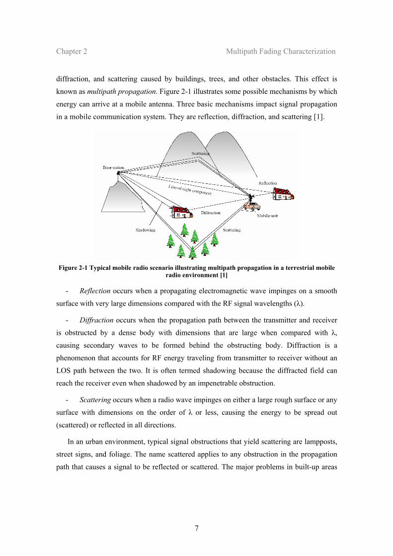
known as multipath propagation. Figure 2-1 illustrates some possible mechanisms by which
energy can arrive at a mobile antenna. Three basic mechanisms impact signal propagation
in a mobile communication system. They are reflection, diffraction, and scattering [1].
Figure 2-1 Typical mobile radio scenario illustrating multipath propagation in a terrestrial mobile
radio environment [1]
- Reflection occurs when a propagating electromagnetic wave impinges on a smooth
surface with very large dimensions compared with the RF signal wavelengths (λ).
- Diffraction occurs when the propagation path between the transmitter and receiver
is obstructed by a dense body with dimensions that are large when compared with λ,
causing secondary waves to be formed behind the obstructing body. Diffraction is a
phenomenon that accounts for RF energy traveling from transmitter to receiver without an
LOS path between the two. It is often termed shadowing because the diffracted field can
reach the receiver even when shadowed by an impenetrable obstruction.
- Scattering occurs when a radio wave impinges on either a large rough surface or any
surface with dimensions on the order of λ or less, causing the energy to be spread out
(scattered) or reflected in all directions.
In an urban environment, typical signal obstructions that yield scattering are lampposts,
street signs, and foliage. The name scattered applies to any obstruction in the propagation
path that causes a signal to be reflected or scattered. The major problems in built-up areas
Chapter 2 Multipath Fading Characterization
10
Moving the receiver by a short distance or any variations at the environment can change
the signal strength by several tens of decibels because the relative movement changes the
phase relationship between the incoming component waves. Substantial variations therefore
occur in the signal amplitude. The signal fluctuations are known as fading. Two types of
fading effects are distinguished that characterize mobile communications: large-scale fading
(slow fading) and small-scale fading (fast fading).
Large-scale fading represents the average signal power attenuation or the path loss
resulting from motion over large areas. Because the variations are caused by the mobile
moving into the shadow of hills, forests, billboards, or clumps of buildings, slow fading is
often called shadowing. Measurements indicate that the mean path loss closely fits a log-
normal distribution with a standard deviation that depends on the frequency and the
environment. For this reason the term log-normal fading is also used.
The short-term fluctuation caused by the local multipath is known as fast fading. Fast
fading refers to the dramatic changes in signal amplitude and phase that can be experienced
as a result of small changes (as small as half wavelengths) in the spatial positioning between
a receiver and a transmitter. Fast fading is called Rayleigh fading if there are multiple
reflective paths that are large in number, and there is no line-of-sight (LOS) signal
component; the central limit theorem can be invoked to model the fast fading by a filtered
complex Gaussian process. The envelope of such a received signal is statistically described
by a Rayleigh probability density function (PDF).
When a dominant non fading signal component present, such as a LOS propagation path,
the statistics of small-scale fading envelope is described by a Rician PDF [2]. In other
words, the small-scale fading statistics are said to be Rayleigh whenever the LOS path is
blocked, and Rician otherwise.
A mobile radio roaming over a large area must process signals that experience both types
of fading: small-scale fading superimposed on large-scale fading. A typical received signal
envelope as a function of distance is shown in Figure 2-4 illustrates this point. The slow
variation in mean signal level, indicated in Figure 2-4 by the dotted line, occurs over much
larger distances. Large-scale fading (attenuation or path loss) can be considered to be a
spatial average over the small scale fluctuations of the signal. It is generally evaluated by
averaging the received signal over at least 10 to 30 wavelengths to decouple the small-scale
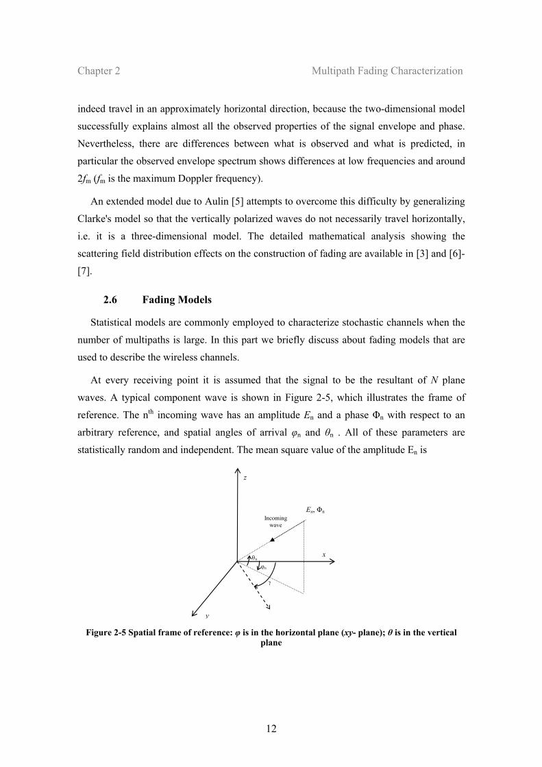
Chapter 2 Multipath Fading Characterization
12
indeed travel in an approximately horizontal direction, because the two-dimensional model
successfully explains almost all the observed properties of the signal envelope and phase.
Nevertheless, there are differences between what is observed and what is predicted, in
particular the observed envelope spectrum shows differences at low frequencies and around
2fm (fm is the maximum Doppler frequency).
An extended model due to Aulin [5] attempts to overcome this difficulty by generalizing
Clarke's model so that the vertically polarized waves do not necessarily travel horizontally,
i.e. it is a three-dimensional model. The detailed mathematical analysis showing the
scattering field distribution effects on the construction of fading are available in [3] and [6]-
[7].
2.6 Fading Models
Statistical models are commonly employed to characterize stochastic channels when the
number of multipaths is large. In this part we briefly discuss about fading models that are
used to describe the wireless channels.
At every receiving point it is assumed that the signal to be the resultant of N plane
waves. A typical component wave is shown in Figure 2-5, which illustrates the frame of
reference. The nth incoming wave has an amplitude En and a phase Φn with respect to an
arbitrary reference, and spatial angles of arrival φn and θn . All of these parameters are
statistically random and independent. The mean square value of the amplitude En is
θn ϕn
y
x
z
Incoming wave
γ
En, Φn
Figure 2-5 Spatial frame of reference: φ is in the horizontal plane (xy- plane); θ is in the vertical
plane
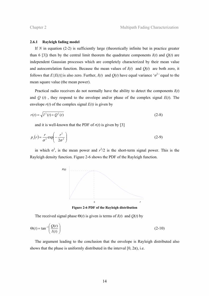
Chapter 2 Multipath Fading Characterization
14
2.6.1 Rayleigh fading model
If N in equation (2-2) is sufficiently large (theoretically infinite but in practice greater
than 6 [3]) then by the central limit theorem the quadrature components I(t) and Q(t) are
independent Gaussian processes which are completely characterized by their mean value
and autocorrelation function. Because the mean values of I(t) and Q(t) are both zero, it
follows that EE(t)is also zero. Further, I(t) and Q(t) have equal variance ‘σ2’ equal to the
mean square value (the mean power).
Practical radio receivers do not normally have the ability to detect the components I(t)
and Q (t) , they respond to the envelope and/or phase of the complex signal E(t). The
envelope r(t) of the complex signal E(t) is given by
)()()( 22 tQtItr += (2-8)
and it is well-known that the PDF of r(t) is given by [3]
( ) ⎟⎟⎠
⎞⎜⎜⎝
⎛−= 2
2
2 2exp
σσrrrpx (2-9)
in which σ2, is the mean power and r2/2 is the short-term signal power. This is the
Rayleigh density function. Figure 2-6 shows the PDF of the Rayleigh function.
r
P(r)
0 Figure 2-6 PDF of the Rayleigh distribution
The received signal phase Θ(t) is given is terms of I(t) and Q(t) by
⎟⎟⎠
⎞⎜⎜⎝
⎛=Θ −
)()(tan)( 1
tItQt (2-10)
The argument leading to the conclusion that the envelope is Rayleigh distributed also
shows that the phase is uniformly distributed in the interval [0, 2π), i.e.
Chapter 2 Multipath Fading Characterization
16
Many different approaches have been used for the modeling and simulation of mobile
radio channels. Among them, the well-known mathematical reference model due to Clarke
[4] and its simplified simulation model due to Jakes [8] have been widely used for Rayleigh
fading channels for about three decades. In this section, we briefly review the mathematical
reference models given for fading channels with the attention on the statistical properties of
the reference model. This information gives the possibility to compare our improved fading
simulator (see chapter 3) with the existent modes.
2.8 Fading Simulator Models
Consider a frequency non-selective fading channel comprised of N propagation paths; and
uniform field scatter in azimuth plane (Clarke’s two dimensional azimuth scattering model)
the low-pass fading process given in equations (2.5) and (2.6) by considering that θn=0,
ωn=ωd cos(γ-φn) are expressed as
( )∑=
+=N
nnndn tEtI
1
coscos)( φαω (2-14)
( )∑=
+=N
nnndn tEtQ
1
cossin)( φαω ( 2-15)
where αn= γ-φn and nφ is uniformly distributed over [0,2π). ωd is the maximum radian
Doppler occurring when αn=0.
Assuming that αn and nφ are mutually independent and uniformly distributed over [0,2π),
some desired second order statistics for fading simulators are manifested in the
autocorrelation and cross-correlation functions as [9]
[ ] )()()()( 0, τωττ dII JtItIER =+= (2-16a)
[ ] )()()()( 0, τωττ dQQ JtQtQER =+= (2-16b)
0,, == QIIQ RR (2-16c)
)(0, τωdrr JR = (2-16e)
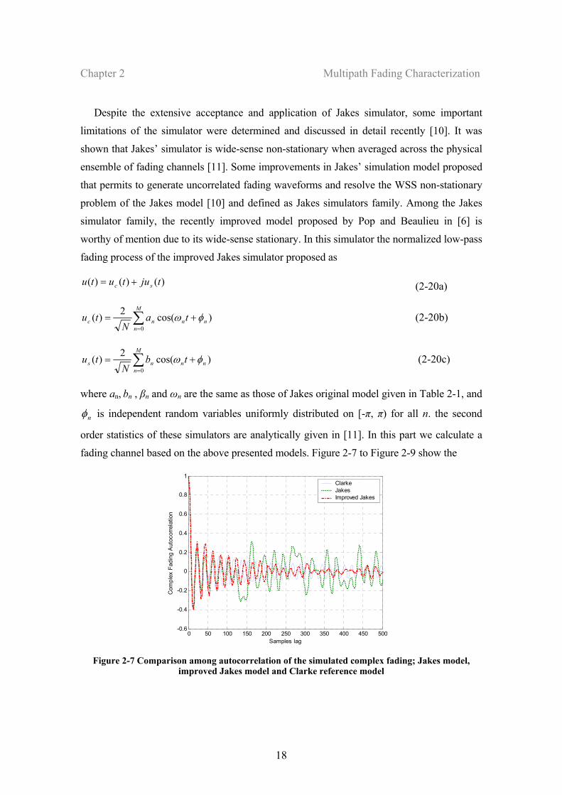
Chapter 2 Multipath Fading Characterization
18
Despite the extensive acceptance and application of Jakes simulator, some important
limitations of the simulator were determined and discussed in detail recently [10]. It was
shown that Jakes’ simulator is wide-sense non-stationary when averaged across the physical
ensemble of fading channels [11]. Some improvements in Jakes’ simulation model proposed
that permits to generate uncorrelated fading waveforms and resolve the WSS non-stationary
problem of the Jakes model [10] and defined as Jakes simulators family. Among the Jakes
simulator family, the recently improved model proposed by Pop and Beaulieu in [6] is
worthy of mention due to its wide-sense stationary. In this simulator the normalized low-pass
fading process of the improved Jakes simulator proposed as
)()()( tjututu sc += (2-20a)
∑=
+=M
nnnnc ta
Ntu
0
)cos(2)( φω (2-20b)
∑=
+=M
nnnns tb
Ntu
0)cos(2)( φω (2-20c)
where an, bn , βn and ωn are the same as those of Jakes original model given in Table 2-1, and
nφ is independent random variables uniformly distributed on [-π, π) for all n. the second
order statistics of these simulators are analytically given in [11]. In this part we calculate a
fading channel based on the above presented models. Figure 2-7 to Figure 2-9 show the
0 50 100 150 200 250 300 350 400 450 500-0.6
-0.4
-0.2
0
0.2
0.4
0.6
0.8
1
Samples lag
Com
plex
Fad
ing
Aut
ocor
rela
tion
ClarkeJakesImproved Jakes
Figure 2-7 Comparison among autocorrelation of the simulated complex fading; Jakes model,
improved Jakes model and Clarke reference model
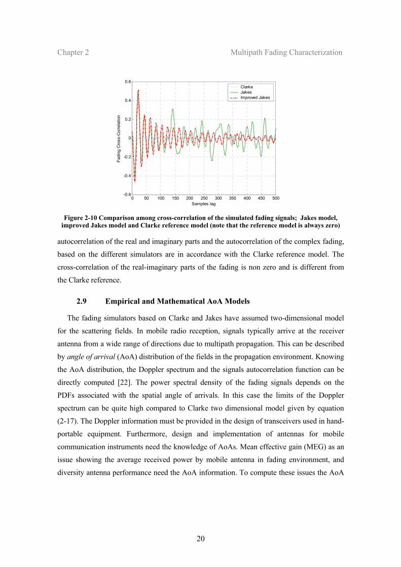
Chapter 2 Multipath Fading Characterization
20
0 50 100 150 200 250 300 350 400 450 500-0.6
-0.4
-0.2
0
0.2
0.4
0.6
Samples lag
Fadi
ng C
ross
-Cor
rela
tion
ClarkeJakesImproved Jakes
Figure 2-10 Comparison among cross-correlation of the simulated fading signals; Jakes model,
improved Jakes model and Clarke reference model (note that the reference model is always zero)
autocorrelation of the real and imaginary parts and the autocorrelation of the complex fading,
based on the different simulators are in accordance with the Clarke reference model. The
cross-correlation of the real-imaginary parts of the fading is non zero and is different from
the Clarke reference.
2.9 Empirical and Mathematical AoA Models
The fading simulators based on Clarke and Jakes have assumed two-dimensional model
for the scattering fields. In mobile radio reception, signals typically arrive at the receiver
antenna from a wide range of directions due to multipath propagation. This can be described
by angle of arrival (AoA) distribution of the fields in the propagation environment. Knowing
the AoA distribution, the Doppler spectrum and the signals autocorrelation function can be
directly computed [22]. The power spectral density of the fading signals depends on the
PDFs associated with the spatial angle of arrivals. In this case the limits of the Doppler
spectrum can be quite high compared to Clarke two dimensional model given by equation
(2-17). The Doppler information must be provided in the design of transceivers used in hand-
portable equipment. Furthermore, design and implementation of antennas for mobile
communication instruments need the knowledge of AoAs. Mean effective gain (MEG) as an
issue showing the average received power by mobile antenna in fading environment, and
diversity antenna performance need the AoA information. To compute these issues the AoA
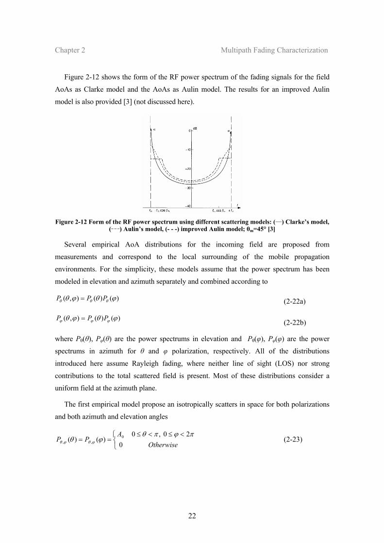
Chapter 2 Multipath Fading Characterization
22
Figure 2-12 shows the form of the RF power spectrum of the fading signals for the field
AoAs as Clarke model and the AoAs as Aulin model. The results for an improved Aulin
model is also provided [3] (not discussed here).
Figure 2-12 Form of the RF power spectrum using different scattering models: (___) Clarke’s model,
(_ _ _) Aulin’s model, (- - -) improved Aulin model; θm=45° [3]
Several empirical AoA distributions for the incoming field are proposed from
measurements and correspond to the local surrounding of the mobile propagation
environments. For the simplicity, these models assume that the power spectrum has been
modeled in elevation and azimuth separately and combined according to
)()(),( ϕθϕθ θθθ PPP = (2-22a)
)()(),( ϕθϕθ ϕϕϕ PPP = (2-22b)
where Pθ(θ), Pφ(θ) are the power spectrums in elevation and Pθ(φ), Pφ(φ) are the power
spectrums in azimuth for θ and φ polarization, respectively. All of the distributions
introduced here assume Rayleigh fading, where neither line of sight (LOS) nor strong
contributions to the total scattered field is present. Most of these distributions consider a
uniform field at the azimuth plane.
The first empirical model propose an isotropically scatters in space for both polarizations
and both azimuth and elevation angles
⎩⎨⎧ <≤<≤
==Otherwise
APP
020,0
)()( 0,,
πϕπθϕθ ϕθϕθ (2-23)
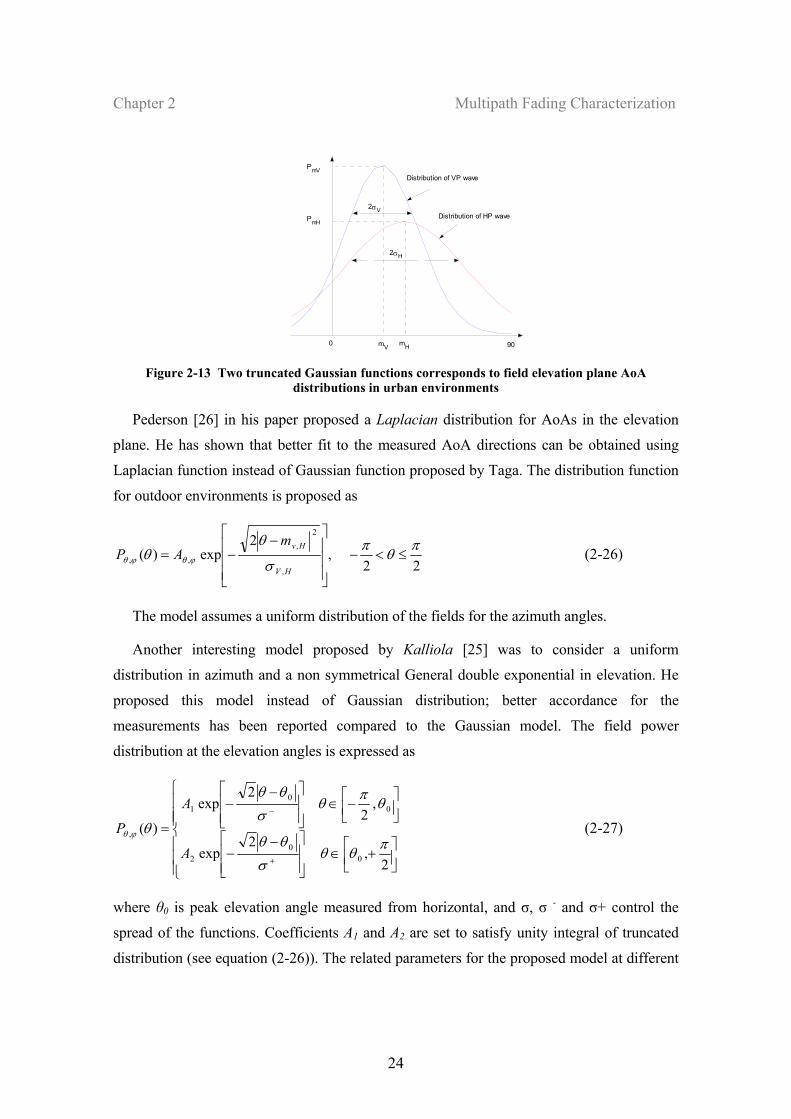
Chapter 2 Multipath Fading Characterization
24
PmV
PmH
mV mH
2σV
2σH
0 90
Distribution of VP wave
Distribution of HP wave
Figure 2-13 Two truncated Gaussian functions corresponds to field elevation plane AoA
distributions in urban environments
Pederson [26] in his paper proposed a Laplacian distribution for AoAs in the elevation
plane. He has shown that better fit to the measured AoA directions can be obtained using
Laplacian function instead of Gaussian function proposed by Taga. The distribution function
for outdoor environments is proposed as
22,
2exp)(
,
2,
,,πθπ
σ
θθ ϕθϕθ ≤<−
⎥⎥⎥
⎦
⎤
⎢⎢⎢
⎣
⎡ −−=
HV
HvmAP (2-26)
The model assumes a uniform distribution of the fields for the azimuth angles.
Another interesting model proposed by Kalliola [25] was to consider a uniform
distribution in azimuth and a non symmetrical General double exponential in elevation. He
proposed this model instead of Gaussian distribution; better accordance for the
measurements has been reported compared to the Gaussian model. The field power
distribution at the elevation angles is expressed as
⎪⎪⎪
⎩
⎪⎪⎪
⎨
⎧
⎥⎦⎤
⎢⎣⎡ +∈
⎥⎥⎦
⎤
⎢⎢⎣
⎡ −−
⎥⎦⎤
⎢⎣⎡−∈
⎥⎥⎦
⎤
⎢⎢⎣
⎡ −−
=
+
−
2,
2exp
,2
2exp
)(
00
2
00
1
,πθθ
σθθ
θπθσ
θθ
θϕθ
A
A
P (2-27)
where θ0 is peak elevation angle measured from horizontal, and σ, σ - and σ+ control the
spread of the functions. Coefficients A1 and A2 are set to satisfy unity integral of truncated
distribution (see equation (2-26)). The related parameters for the proposed model at different
Chapter 2 Multipath Fading Characterization
26
where aθ1 and bθ1 are the axial ratios of the ellipsis and bθ0 gives the directivity towards the
windows. A similar distribution is assumed for the horizontal polarization with
corresponding parameters aφ1, bφ1, bφ0 and Aφ. It is observed that a uniform distribution is a
special case of the elliptical model. Due to the measurements performed by Knudsen [27] the
elliptical parameters are given as:
18.1,46.0,98.012.2,70.0,71.0
101
101
======
φφφ
θθθ
bbabba
(2-28b)
Furthermore, in this model the field power distribution in elevation plane was considered as
Gaussian distribution.
In this thesis the above propagation models have been applied to cover as much as
possible of the indoor, outdoor and outdoor to indoor propagation scenarios. The models are
used for the mean effective gain and diversity performance factors evaluation. Table 2-3
summarizes the applied propagation models in this thesis. M1 corresponds to Clarke 2-D
model with AoA in azimuth plane only. M2 corresponds to a model with uniform field
distribution in azimuth plane and Gaussian in elevation (Gaussian parameters given in Table
2-3 correspond to Taga’s model); M3 considers a uniform distribution in azimuth plane and
Double exponential in elevation the related parameters are depicted in Table 2-2. M4
supposes an elliptical distribution in azimuth plane with maximum value toward the building
opening and Gaussian distribution in elevation plane. The Gaussian parameters can be
adjusted as Taga model.
Figure 2-14a-d illustrate the incident field AoA distributions given in Table 2-3.
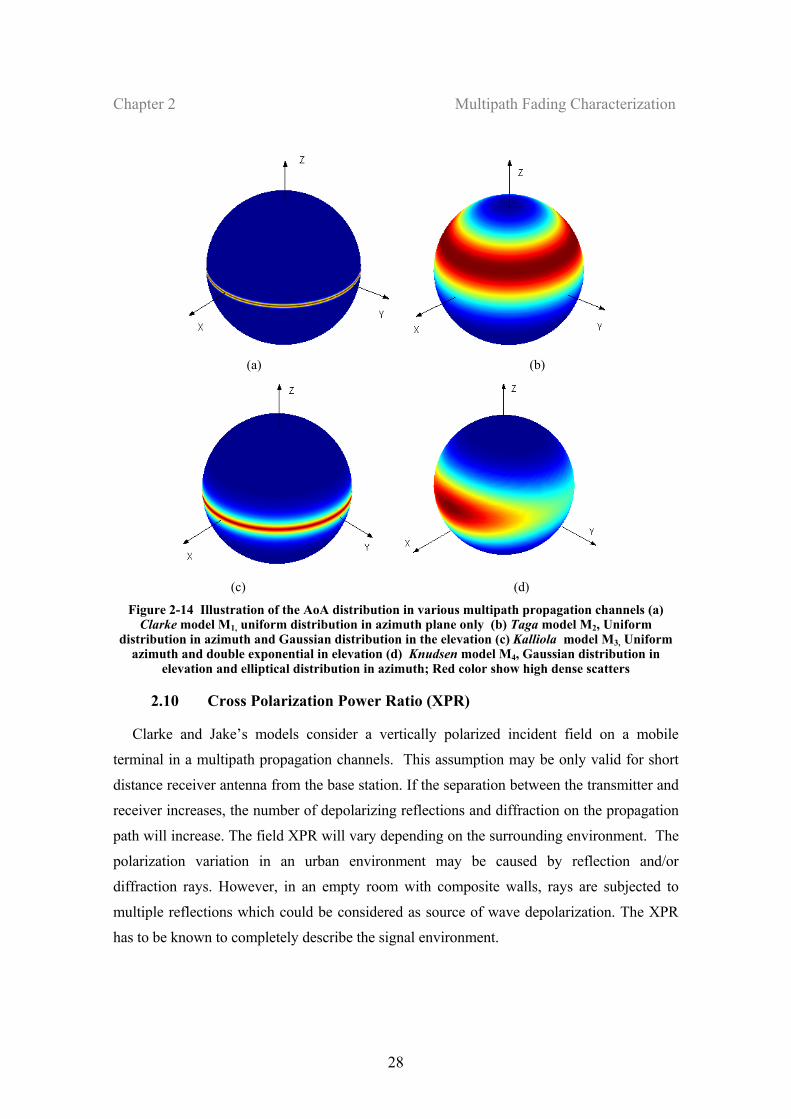
Chapter 2 Multipath Fading Characterization
28
(a) (b)
(c) (d)
Figure 2-14 Illustration of the AoA distribution in various multipath propagation channels (a) Clarke model M1, uniform distribution in azimuth plane only (b) Taga model M2, Uniform
distribution in azimuth and Gaussian distribution in the elevation (c) Kalliola model M3, Uniform azimuth and double exponential in elevation (d) Knudsen model M4, Gaussian distribution in
elevation and elliptical distribution in azimuth; Red color show high dense scatters
2.10 Cross Polarization Power Ratio (XPR)
Clarke and Jake’s models consider a vertically polarized incident field on a mobile
terminal in a multipath propagation channels. This assumption may be only valid for short
distance receiver antenna from the base station. If the separation between the transmitter and
receiver increases, the number of depolarizing reflections and diffraction on the propagation
path will increase. The field XPR will vary depending on the surrounding environment. The
polarization variation in an urban environment may be caused by reflection and/or
diffraction rays. However, in an empty room with composite walls, rays are subjected to
multiple reflections which could be considered as source of wave depolarization. The XPR
has to be known to completely describe the signal environment.
Chapter 2 Multipath Fading Characterization
30
influence on the XPR. In the highway macrocell measurements, the close scattering from the
bodywork of the car most probably decreases the XPR. The XPR decreased to 0dB at sites
surrounded by tall buildings [24].
2.11 Mean Effective Gain (MEG)
Mean Effective Gain is a parameter which shows the performance of an antenna system
in relation with the scattering field environment. It is defined as the ratio of the average
power received by an antenna in a random scattering field environment to the total average
power incident to the antenna in the same environment. The total power is the summation of
vertical and horizontal polarized powers that receive by an isotropic antenna. A general
formulation for the MEG is expressed as
HV
c
PPP
MEG+
= Re (2-30)
where cPRe is the average power received at the antenna, vP and HP are the vertical and
horizontal polarized waves received by an isotropic antenna at the same environment of the
antenna under test. MEG contains the mutual effect between the antenna power gain pattern
and the propagation characteristics of the multipath scenario.
Under the assumption that the incident field on the antenna is composed of two
uncorrelated vertical and horizontal components, both of a Rayleigh distribution, the
received power by an antenna in this environment is given by
∫ΩΩΩΩΩ+ΩΩ= ),(,)()()()(Re ϕθϕϕθθ dPGPPGPP HVc ( 2-31)
where Ω(θ,φ) is the spatial angles in steradian; dΩ=sinθ dθ dφ and Gφ(Ω), Gθ(Ω) are the
antenna power gains for φ-polarized and θ-polarized field components, respectively; Pv and
PH are the mean incident powers in vertical and horizontal polarizations, respectively.
Pθ(Ω) and Pφ(Ω) are the θ-polarized and φ-polarized components of the angular power
density functions of the incoming waves assume the normalization in (2-24).
By dividing the received power of the antenna under test to the incident power on the
antenna the mean effective gain is then determined using (2-30) and (2-33) [24],[31] as
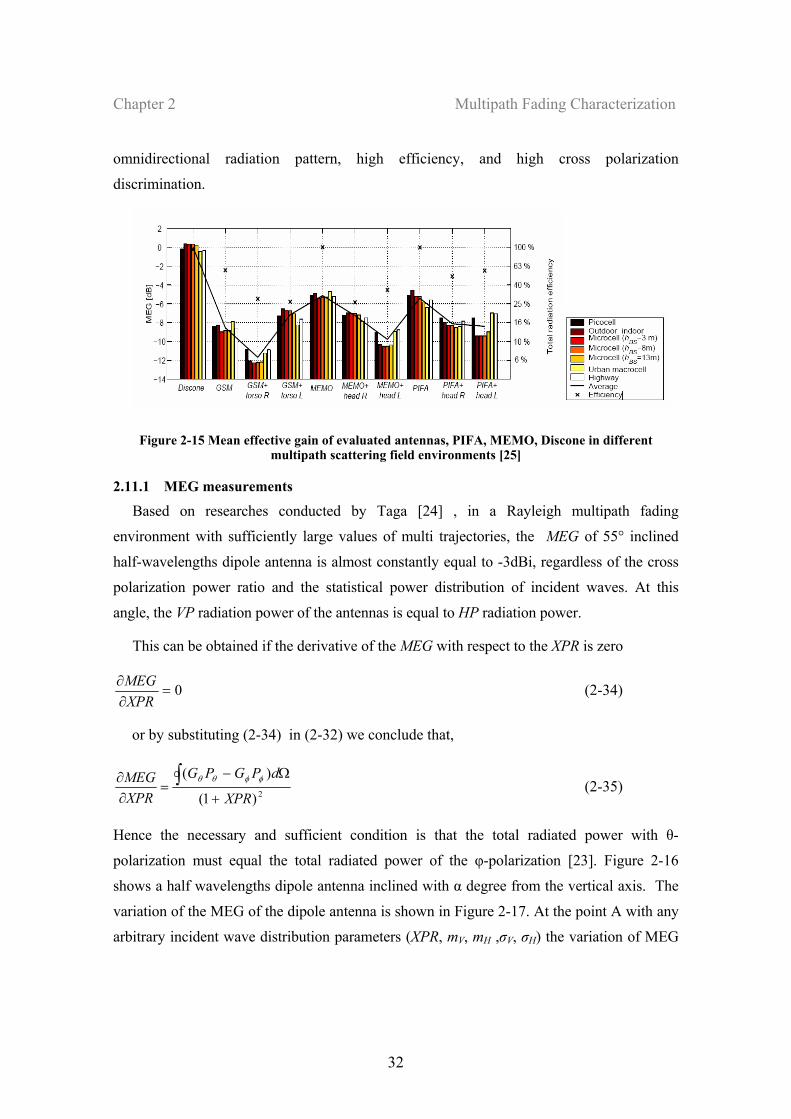
Chapter 2 Multipath Fading Characterization
32
omnidirectional radiation pattern, high efficiency, and high cross polarization
discrimination.
Figure 2-15 Mean effective gain of evaluated antennas, PIFA, MEMO, Discone in different multipath scattering field environments [25]
2.11.1 MEG measurements
Based on researches conducted by Taga [24] , in a Rayleigh multipath fading
environment with sufficiently large values of multi trajectories, the MEG of 55° inclined
half-wavelengths dipole antenna is almost constantly equal to -3dBi, regardless of the cross
polarization power ratio and the statistical power distribution of incident waves. At this
angle, the VP radiation power of the antennas is equal to HP radiation power.
This can be obtained if the derivative of the MEG with respect to the XPR is zero
0=∂∂
XPRMEG (2-34)
or by substituting (2-34) in (2-32) we conclude that,
2)1(
)(
XPR
dPGPG
XPRMEG
+
Ω−=
∂∂ ∫ φφθθ (2-35)
Hence the necessary and sufficient condition is that the total radiated power with θ-
polarization must equal the total radiated power of the φ-polarization [23]. Figure 2-16
shows a half wavelengths dipole antenna inclined with α degree from the vertical axis. The
variation of the MEG of the dipole antenna is shown in Figure 2-17. At the point A with any
arbitrary incident wave distribution parameters (XPR, mV, mH ,σV, σH) the variation of MEG
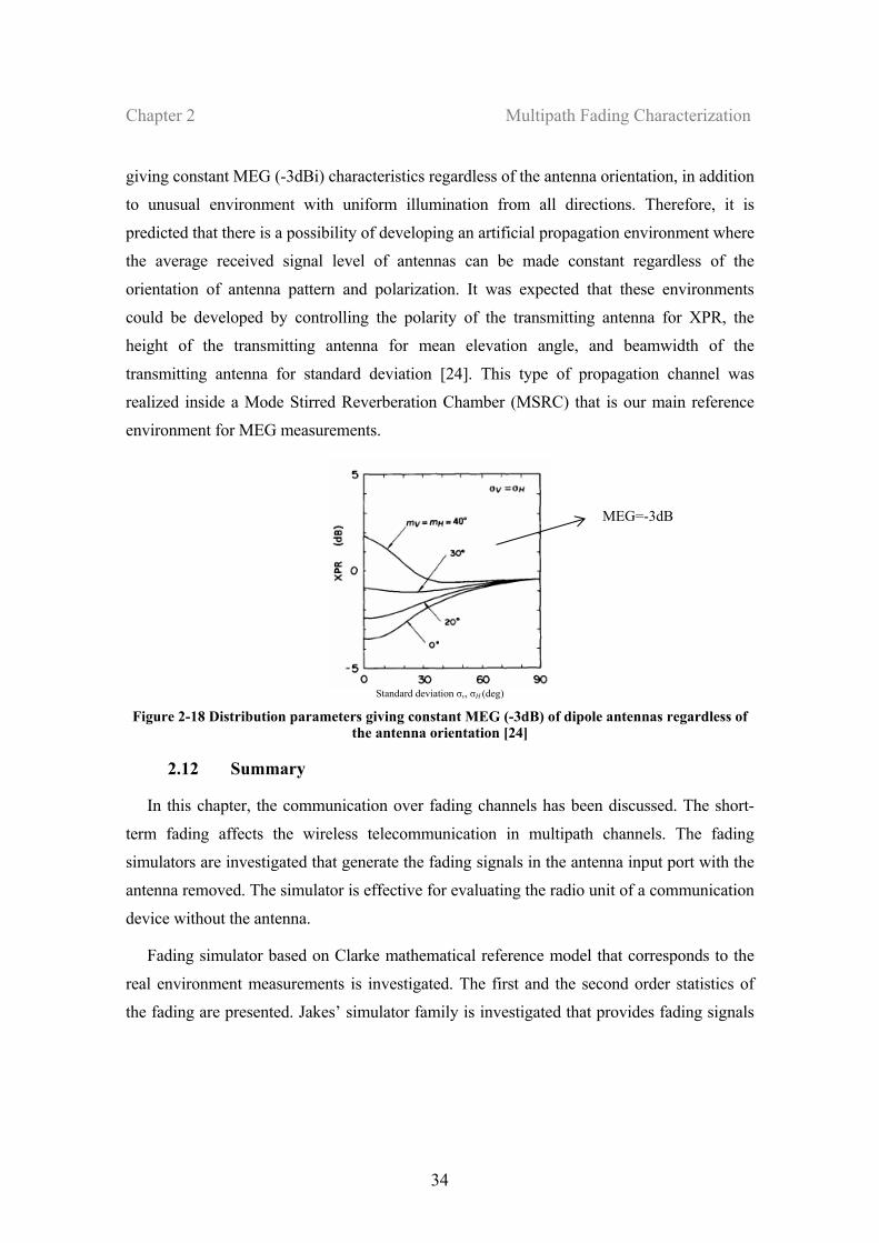
Chapter 2 Multipath Fading Characterization
34
giving constant MEG (-3dBi) characteristics regardless of the antenna orientation, in addition
to unusual environment with uniform illumination from all directions. Therefore, it is
predicted that there is a possibility of developing an artificial propagation environment where
the average received signal level of antennas can be made constant regardless of the
orientation of antenna pattern and polarization. It was expected that these environments
could be developed by controlling the polarity of the transmitting antenna for XPR, the
height of the transmitting antenna for mean elevation angle, and beamwidth of the
transmitting antenna for standard deviation [24]. This type of propagation channel was
realized inside a Mode Stirred Reverberation Chamber (MSRC) that is our main reference
environment for MEG measurements.
Standard deviation σv, σH (deg)
Figure 2-18 Distribution parameters giving constant MEG (-3dB) of dipole antennas regardless of the antenna orientation [24]
2.12 Summary
In this chapter, the communication over fading channels has been discussed. The short-
term fading affects the wireless telecommunication in multipath channels. The fading
simulators are investigated that generate the fading signals in the antenna input port with the
antenna removed. The simulator is effective for evaluating the radio unit of a communication
device without the antenna.
Fading simulator based on Clarke mathematical reference model that corresponds to the
real environment measurements is investigated. The first and the second order statistics of
the fading are presented. Jakes’ simulator family is investigated that provides fading signals
MEG=-3dB
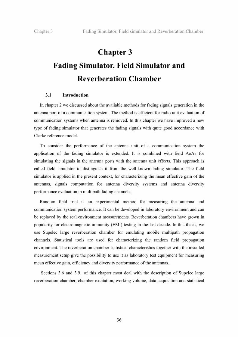
Chapter 3 Fading Simulator, Field simulator and Reverberation Chamber
36
Chapter 3
Fading Simulator, Field Simulator and
Reverberation Chamber
3.1 Introduction
In chapter 2 we discussed about the available methods for fading signals generation in the
antenna port of a communication system. The method is efficient for radio unit evaluation of
communication systems when antenna is removed. In this chapter we have improved a new
type of fading simulator that generates the fading signals with quite good accordance with
Clarke reference model.
To consider the performance of the antenna unit of a communication system the
application of the fading simulator is extended. It is combined with field AoAs for
simulating the signals in the antenna ports with the antenna unit effects. This approach is
called field simulator to distinguish it from the well-known fading simulator. The field
simulator is applied in the present context, for characterizing the mean effective gain of the
antennas, signals computation for antenna diversity systems and antenna diversity
performance evaluation in multipath fading channels.
Random field trial is an experimental method for measuring the antenna and
communication system performance. It can be developed in laboratory environment and can
be replaced by the real environment measurements. Reverberation chambers have grown in
popularity for electromagnetic immunity (EMI) testing in the last decade. In this thesis, we
use Supelec large reverberation chamber for emulating mobile multipath propagation
channels. Statistical tools are used for characterizing the random field propagation
environment. The reverberation chamber statistical characteristics together with the installed
measurement setup give the possibility to use it as laboratory test equipment for measuring
mean effective gain, efficiency and diversity performance of the antennas.
Sections 3.6 and 3.9 of this chapter most deal with the description of Supelec large
reverberation chamber, chamber excitation, working volume, data acquisition and statistical
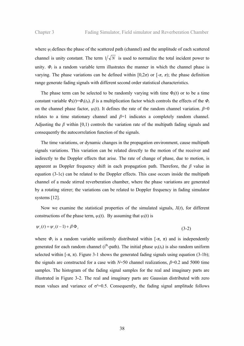
Chapter 3 Fading Simulator, Field simulator and Reverberation Chamber
38
where ψi defines the phase of the scattered path (channel) and the amplitude of each scattered
channel is unity constant. The term N1 is used to normalize the total incident power to
unity. Φi is a random variable term illustrates the manner in which the channel phase is
varying. The phase variations can be defined within [0,2π) or [-π, π); the phase definition
range generate fading signals with different second order statistical characteristics.
The phase term can be selected to be randomly varying with time Φi(t) or to be a time
constant variable Φi(t)=Φi(t0). β is a multiplication factor which controls the effects of the Φi
on the channel phase factor, ψi(t). It defines the rate of the random channel variation. β=0
relates to a time stationary channel and β=1 indicates a completely random channel.
Adjusting the β within [0,1) controls the variation rate of the multipath fading signals and
consequently the autocorrelation function of the signals.
The time variations, or dynamic changes in the propagation environment, cause multipath
signals variations. This variation can be related directly to the motion of the receiver and
indirectly to the Doppler effects that arise. The rate of change of phase, due to motion, is
apparent as Doppler frequency shift in each propagation path. Therefore, the β value in
equation (3-1c) can be related to the Doppler effects. This case occurs inside the multipath
channel of a mode stirred reverberation chamber, where the phase variations are generated
by a rotating stirrer; the variations can be related to Doppler frequency in fading simulator
systems [12].
Now we examine the statistical properties of the simulated signals, X(t), for different
constructions of the phase term, ψi(t). By assuming that ψi(t) is
iii tt Φ+−= βψψ )1()( (3-2)
where Φi is a random variable uniformly distributed within [-π, π) and is independently
generated for each random channel (ith-path). The initial phase ψi(t0) is also random uniform
selected within [-π, π). Figure 3-1 shows the generated fading signals using equation (3-1b);
the signals are constructed for a case with N=50 channel realizations, β=0.2 and 5000 time
samples. The histogram of the fading signal samples for the real and imaginary parts are
illustrated in Figure 3-2. The real and imaginary parts are Gaussian distributed with zero
mean values and variance of σ²=0.5. Consequently, the fading signal amplitude follows
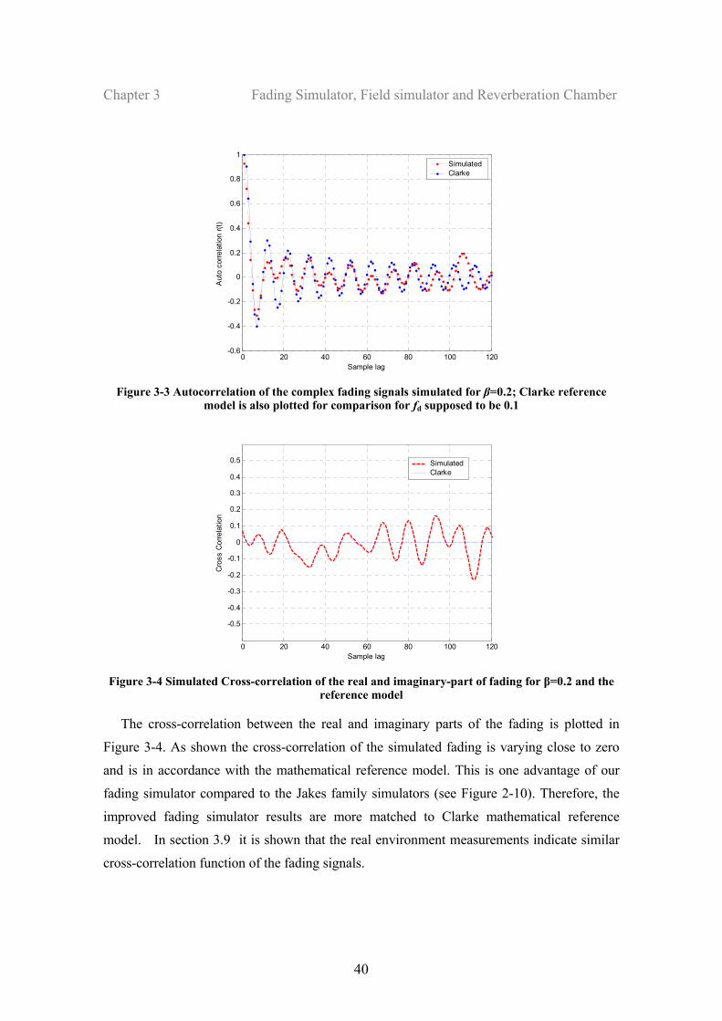
Chapter 3 Fading Simulator, Field simulator and Reverberation Chamber
40
0 20 40 60 80 100 120-0.6
-0.4
-0.2
0
0.2
0.4
0.6
0.8
1
Sample lag
Aut
o co
rrela
tion
r(t)
SimulatedClarke
Figure 3-3 Autocorrelation of the complex fading signals simulated for β=0.2; Clarke reference
model is also plotted for comparison for fd supposed to be 0.1
0 20 40 60 80 100 120
-0.5
-0.4
-0.3
-0.2
-0.1
0
0.1
0.2
0.3
0.4
0.5
Sample lag
Cro
ss C
orre
latio
n
SimulatedClarke
Figure 3-4 Simulated Cross-correlation of the real and imaginary-part of fading for β=0.2 and the
reference model
The cross-correlation between the real and imaginary parts of the fading is plotted in
Figure 3-4. As shown the cross-correlation of the simulated fading is varying close to zero
and is in accordance with the mathematical reference model. This is one advantage of our
fading simulator compared to the Jakes family simulators (see Figure 2-10). Therefore, the
improved fading simulator results are more matched to Clarke mathematical reference
model. In section 3.9 it is shown that the real environment measurements indicate similar
cross-correlation function of the fading signals.
Chapter 3 Fading Simulator, Field simulator and Reverberation Chamber
42
0 5 10 15 20 25 30 35 40-1
-0.8
-0.6
-0.4
-0.2
0
0.2
0.4
0.6
0.8
1
Time lag
Cro
ss-c
orre
latio
n
β=0.1β=0.2β=0.3β=0.4β=0.5
Figure 3-6 Simulated cross-correlation of the fading signal for β=0.1, 0.2, 0.3, 0.4, 0.5 versus time
lag
Among the above proposed fading signals simulation the first method is selected that is
more compatible with real environment measurement. The simulator is used in chapter 4 for
generating multiple fading signals with a pre-defined signals correlation coefficient. The
computed signals are applied to investigate the performance of diversity gain in multi-
antenna receiving systems.
3.3 Field Simulator
Using the fading simulator described in the previous section, the characteristics of
wireless equipment can be evaluated by inputting a fading wave to the antenna input port
with the antenna removed. The test is effective for evaluating the radio unit of a
communication device without the antenna. However, it is also necessary to confirm the
characteristics of the product with the antenna included. In the fading signal simulator the
multipath is generated and summed over channels in order to produce the received signal. If
the antenna is included in the channel path, depending on the channel spatial direction,
different gain and phase values will be applied to each channel. In fact, the antenna will work
as a spatial filter with a gain and phase value proportional to the antenna farfield pattern. If
the multipath signals pass through the radiation pattern the received signal will include the
mutual effect of the channel and antenna unit. In this section we review the available
simulation methods for evaluating the received signals by an antenna in a multipath channel.
Chapter 3 Fading Simulator, Field simulator and Reverberation Chamber
44
where )(ΩAEθ and )(ΩAEϕ are the antenna complex farfield patterns for θ-polarized and φ-
polarized field components, respectively. The antenna pattern can be modeled using
electromagnetic full-wave solutions or can be measured inside an anechoic chamber. To
provide a reference for the received signal power, the incident field on the antenna is
normalized and provides unity radiated power on the antenna
1)()()()( **=ΩΩΩ=ΩΩΩ ∫∫
ΩΩ
dEEdEE iiiiϕϕθθ (3-6)
and the antenna power patterns are normalized to isotropic
πϕϕθθ4)().()().( ** =ΩΩΩ+ΩΩ∫
Ω
dEEEE AAA ( 3-7)
By the present pattern normalization, the effects of the antenna radiation efficiency on the
received signal powers are removed.
The received signal by an antenna is a function of both the incident field and the antenna
farfield radiation patterns. The antenna radiation pattern is weakly affected by the
surrounding environment if sufficiently large distance between the antenna and the
surrounding obstacles are considered. For a mobile handheld device, the user head and hand
are close to the antenna and both changes the radiation pattern, considerably. Therefore, to
have a good estimation of the signals received through an antenna the pattern should be
evaluated regarding to the surrounding environment effects. Considering that the antenna
pattern is evaluated rigorously in relation with the near environments and no pattern changes
are made by the obstacles, we could conclude that the received signal variations by the time
at the antenna port is directly influenced by the environment temporal variations or by the
antenna displacement in different locations.
To simulate the random multipath signals received at an antenna port one method is
proposed by Rice [20] that was based on a developed propagation model [21]. This model
provides the statistical characterizations of the number, amplitude, time-delay, and arrival
angle of the different components of the multipath signal. Using a Monte Carlo approach,
random variables were generated based upon the model for each of the four parameters
mentioned above. Each multipath component was then treated as a plane wave whose
direction of propagation, amplitude, and phase were controlled by the appropriate random
Chapter 3 Fading Simulator, Field simulator and Reverberation Chamber
46
θθθ
ψθ
ˆ)(),( ),( tji ertE Ω−Ω=Ω (3-9a)
ϕϕϕ
ψϕ ˆ)(),( ),( tji ertE Ω−Ω=Ω
(3.9b)
where rθ(Ω) and rφ(Ω) are the spatial distributions of the field angle of arrivals that are
normalized as (3-6) and provide unity incident field power onto the antenna.
To generate a time variable scattered field and consequently a fading signal at the antenna
port, we apply the temporal variations onto the phase factor ψθ,φ(Ω,t). By this method, a
random phase is constructed in Ω space that is uniformly distributed within [0,2π); the phase
factor changes randomly in the time domain. For instance, the phase variation can follow the
proposed fading simulator models as (3-1).
By applying the temporal variations of the phase to equation (3-9), the incident field
magnitude for each spatial field trajectory it always constant and is equal to r(Ω). In that case
the total incident field power on the antenna is determined by r(Ω) distribution. Using this
method, each multipath component was then treated as a plane wave whose direction of
propagation and amplitude are known and the phase is controlled by an appropriate random
variables.
The received signal by an antenna in the generated multipath scenario is obtained by
multiplying each component by the complex pattern at the appropriate angle and summing
the resulting complex components. Normally, the radiation patterns of the antennas can be
simulated or measured with a defined angular resolution for spatial angles. Therefore, the
integral equation (3-5) that expresses the antenna signals for continues evaluated patterns can
be constructed for discrete case as
( )∑∑= =
+=N
n
L
llnl
Aknl
inl
Aknl
ikc EtEEtE
LNtX
1 1
** sin),().,,(),().,,(2)( θφθφθφθφθππϕϕθθ
( 3-10)
whereLl
lπθ = ,
Nnn
πφ 2= and L, N are the number of channels in the elevation and azimuth
planes, respectively. L and N must be selected equal to the resolution of the simulated or
measured patterns. Ei(θl, nφ ) is the incident field in θl and nφ directions and EA(θl, nφ ) is the
antenna farfield pattern in the related directions. The incident field models are given by
equation (3-9). The field amplitude is constant and is defined by the field AoA models; the
Chapter 3 Fading Simulator, Field simulator and Reverberation Chamber
48
relative power can thus be calculated. If the measurements are performed with an operator
holding the terminal antenna, the effects of the human body on the measurement are also
taken into account. This measurement is thus effective for testing communication devices
such as those used on real applications.
The above test and measurements in outdoor environments requires only a suitable
transmitting and receiver system and appropriate site of testing. However, the uncertainty of
weather conditions from day to day and also the need to obtain a testing license for use of
high power transmitter outdoors, makes outdoor testing of mobile terminal troublesome. To
overcome these obstacles, a random field measurement system has been developed for
indoor usage. The indoor testing method is also good a first test of the AUT before moving
on to the final outdoor test.
Figure 3-7 shows a typical indoor measurement setup. The measurement environment is
an office/laboratory. The receivers and transmitters are placed at locations marked as Rx, Tx,
respectively. Depending on the surrounding furniture, equipment, cabling, the office walls
material and shaping, the floor, pillars and outdoor walls, the ceiling and the materials, the
placement of the transmitter and receiver different multipath channels are generated. The
transmitter is fixed and transmits the signals at the measurement frequency, the receiver
(AUT) can be moved in a straight path inside the room or can be rotated around a fixed
point. The moving antenna will experience various multipath channels and the measurement
can be repeated by periodically movement of the AUT. Ideally, a measuring device with the
same number of ports as antennas is needed to measure simultaneously the signals for
estimate the multi antenna system performance. Normal network analyzers only have two
ports; so a multiplexing system for measuring more than two ports is needed. This is because
the terminal may be moving during sampling time and the scattering environment may be
changing. Time- multiplexed measurements are acceptable for a static situation in which the
scattering environment is unchanging and the terminal remains still over the sample time
[32].
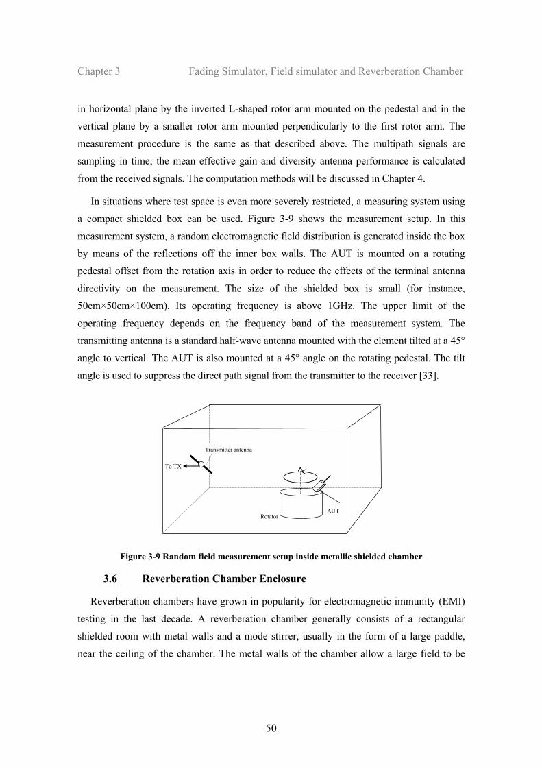
Chapter 3 Fading Simulator, Field simulator and Reverberation Chamber
50
in horizontal plane by the inverted L-shaped rotor arm mounted on the pedestal and in the
vertical plane by a smaller rotor arm mounted perpendicularly to the first rotor arm. The
measurement procedure is the same as that described above. The multipath signals are
sampling in time; the mean effective gain and diversity antenna performance is calculated
from the received signals. The computation methods will be discussed in Chapter 4.
In situations where test space is even more severely restricted, a measuring system using
a compact shielded box can be used. Figure 3-9 shows the measurement setup. In this
measurement system, a random electromagnetic field distribution is generated inside the box
by means of the reflections off the inner box walls. The AUT is mounted on a rotating
pedestal offset from the rotation axis in order to reduce the effects of the terminal antenna
directivity on the measurement. The size of the shielded box is small (for instance,
50cm×50cm×100cm). Its operating frequency is above 1GHz. The upper limit of the
operating frequency depends on the frequency band of the measurement system. The
transmitting antenna is a standard half-wave antenna mounted with the element tilted at a 45°
angle to vertical. The AUT is also mounted at a 45° angle on the rotating pedestal. The tilt
angle is used to suppress the direct path signal from the transmitter to the receiver [33].
AUT
Transmitter antenna
To TX
Rotator
Figure 3-9 Random field measurement setup inside metallic shielded chamber
3.6 Reverberation Chamber Enclosure
Reverberation chambers have grown in popularity for electromagnetic immunity (EMI)
testing in the last decade. A reverberation chamber generally consists of a rectangular
shielded room with metal walls and a mode stirrer, usually in the form of a large paddle,
near the ceiling of the chamber. The metal walls of the chamber allow a large field to be
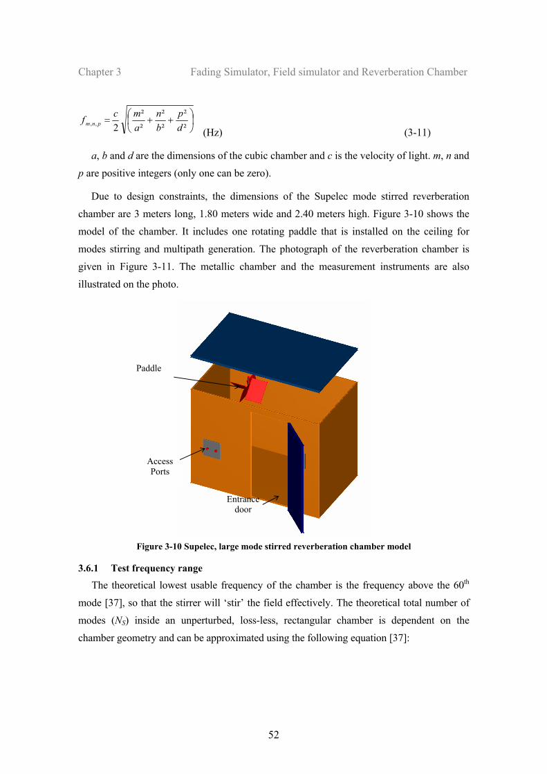
Chapter 3 Fading Simulator, Field simulator and Reverberation Chamber
52
⎟⎠⎞
⎜⎝⎛ ++=
²²
²²
²²
2,, dp
bn
amcf pnm
(Hz) (3-11)
a, b and d are the dimensions of the cubic chamber and c is the velocity of light. m, n and
p are positive integers (only one can be zero).
Due to design constraints, the dimensions of the Supelec mode stirred reverberation
chamber are 3 meters long, 1.80 meters wide and 2.40 meters high. Figure 3-10 shows the
model of the chamber. It includes one rotating paddle that is installed on the ceiling for
modes stirring and multipath generation. The photograph of the reverberation chamber is
given in Figure 3-11. The metallic chamber and the measurement instruments are also
illustrated on the photo.
Figure 3-10 Supelec, large mode stirred reverberation chamber model
3.6.1 Test frequency range
The theoretical lowest usable frequency of the chamber is the frequency above the 60th
mode [37], so that the stirrer will ‘stir’ the field effectively. The theoretical total number of
modes (NS) inside an unperturbed, loss-less, rectangular chamber is dependent on the
chamber geometry and can be approximated using the following equation [37]:
Paddle
Access Ports
Entrance door
Chapter 3 Fading Simulator, Field simulator and Reverberation Chamber
54
3.6.2 Antennas
In order to reduce the direct coupling path between the antennas and to maximize the field
perturbation, the transmitting antenna (which produces the electromagnetic fields within the
chamber) can be directed at the mode stirrer or into the corner of the chamber [38]. Direct
coupling is also reduced if the antennas are not too close together and do not face each other
[38].
3.6.3 Working volume
The working volume is the volume inside which the statistical properties of the MSRC,
i.e. homogeneity and isotropy, are respected. As the stirrer rotates, the maximum field
obtained during one rotation of the stirrer is the same at any point (greater than 0.5
wavelengths from the chambers walls, floor and ceiling) in the room, this volume is referred
to as the working volume. The working volume can be found by placing the receiving
antenna or a field probe in various positions and monitoring the field strength over one
revolution. The actual working volume is determined with a field monitoring probe. This
probe is used to measure the field strength at any given point within the chamber. After the
field strength has been determined for all stirrer positions and various probe positions,
calculations can be performed to determine whether the field is statistically uniform at those
points for valid tests to be performed and the precise working volume for each frequency can
be found.
3.6.4 Mode modification techniques
The previous analysis for the number of modes and working frequency were considered
a rectangular cubic MSRC without any stirring paddle inside. The performance of the
chamber is also depending on the performance of the mode stirrer. The mode stirrer
techniques have been investigated such as:
- Rectangular chamber with wall angle irregularities: the intrinsic reverberation
chamber (IRC) [39]
- Wall irregularities, such as the phase reflection gratings [40, 41], Schroeder
diffusers [42] or corrugated walls [43]
- Moving wall [44]
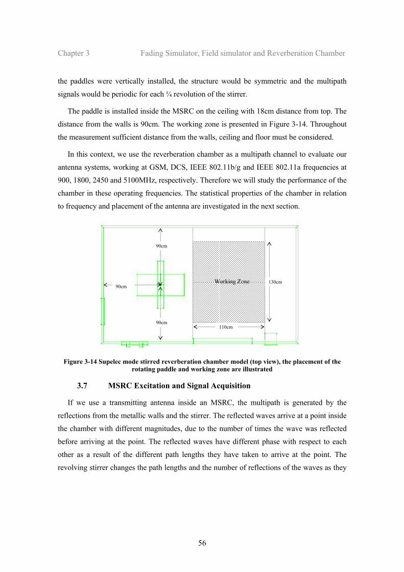
Chapter 3 Fading Simulator, Field simulator and Reverberation Chamber
56
the paddles were vertically installed, the structure would be symmetric and the multipath
signals would be periodic for each ¼ revolution of the stirrer.
The paddle is installed inside the MSRC on the ceiling with 18cm distance from top. The
distance from the walls is 90cm. The working zone is presented in Figure 3-14. Throughout
the measurement sufficient distance from the walls, ceiling and floor must be considered.
In this context, we use the reverberation chamber as a multipath channel to evaluate our
antenna systems, working at GSM, DCS, IEEE 802.11b/g and IEEE 802.11a frequencies at
900, 1800, 2450 and 5100MHz, respectively. Therefore we will study the performance of the
chamber in these operating frequencies. The statistical properties of the chamber in relation
to frequency and placement of the antenna are investigated in the next section.
90cm
90cm
90cm
Working Zone
110cm
130cm
Figure 3-14 Supelec mode stirred reverberation chamber model (top view), the placement of the
rotating paddle and working zone are illustrated
3.7 MSRC Excitation and Signal Acquisition
If we use a transmitting antenna inside an MSRC, the multipath is generated by the
reflections from the metallic walls and the stirrer. The reflected waves arrive at a point inside
the chamber with different magnitudes, due to the number of times the wave was reflected
before arriving at the point. The reflected waves have different phase with respect to each
other as a result of the different path lengths they have taken to arrive at the point. The
revolving stirrer changes the path lengths and the number of reflections of the waves as they
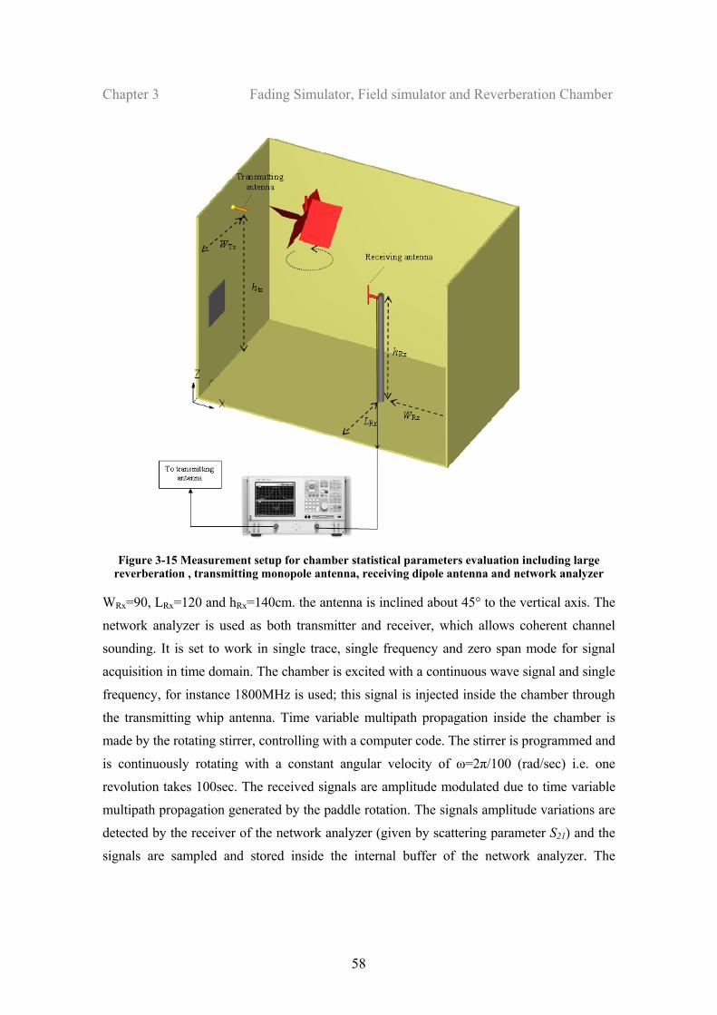
Chapter 3 Fading Simulator, Field simulator and Reverberation Chamber
58
Figure 3-15 Measurement setup for chamber statistical parameters evaluation including large
reverberation , transmitting monopole antenna, receiving dipole antenna and network analyzer
WRx=90, LRx=120 and hRx=140cm. the antenna is inclined about 45° to the vertical axis. The
network analyzer is used as both transmitter and receiver, which allows coherent channel
sounding. It is set to work in single trace, single frequency and zero span mode for signal
acquisition in time domain. The chamber is excited with a continuous wave signal and single
frequency, for instance 1800MHz is used; this signal is injected inside the chamber through
the transmitting whip antenna. Time variable multipath propagation inside the chamber is
made by the rotating stirrer, controlling with a computer code. The stirrer is programmed and
is continuously rotating with a constant angular velocity of ω=2π/100 (rad/sec) i.e. one
revolution takes 100sec. The received signals are amplitude modulated due to time variable
multipath propagation generated by the paddle rotation. The signals amplitude variations are
detected by the receiver of the network analyzer (given by scattering parameter S21) and the
signals are sampled and stored inside the internal buffer of the network analyzer. The
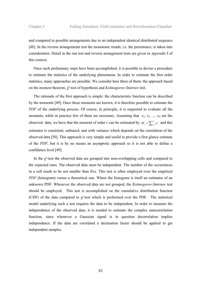
Chapter 3 Fading Simulator, Field simulator and Reverberation Chamber
62
and compared to possible arrangements due to an independent identical distributed sequence
[48]. In the reverse arrangements test the monotonic trends, i.e. the persistence, is taken into
consideration. Detail in the run test and reverse arrangement tests are given in Appendix I of
this context.
Once such preliminary steps have been accomplished, it is possible to devise a procedure
to estimate the statistics of the underlying phenomena. In order to estimate the first order
statistics, many approaches are possible. We consider here three of them: the approach based
on the moment theorem, χ²-test of hypothesis and Kolmogorov-Smirnov test.
The rationale of the first approach is simple: the characteristic function can be described
by the moments [49]. Once these moments are known, it is therefore possible to estimate the
PDF of the underlying process. Of course, in principle, it is requested to evaluate all the
moments, while in practice few of them are necessary. Assuming that x1, x2, …, xN are the
observed data, we have that the moment of order r can be estimated by ∑ ==
N
irir xM
1 and this
estimator is consistent, unbiased, and with variance which depends on the correlation of the
observed data [50]. This approach is very simple and useful to provide a first glance estimate
of the PDF, but it is by no means an asymptotic approach so it is not able to define a
confidence level [49].
In the χ²-test the observed data are grouped into non-overlapping cells and compared to
the expected ones. The observed data must be independent. The number of the occurrences
in a cell needs to be not smaller than five. This test is often employed over the empirical
PDF (histogram) versus a theoretical one. Where the histogram is itself an estimator of an
unknown PDF. Whenever the observed data are not grouped, the Kolmogorov-Smirnov test
should be employed. This test is accomplished on the cumulative distribution function
(CDF) of the data compared to χ²-test which is performed over the PDF. The statistical
model underlying such a test requires the data to be independent. In order to measure the
independence of the observed data, it is needed to estimate the complex autocorrelation
function, since whenever a Gaussian signal is in question decorrelation implies
independence. If the data are correlated a decimation factor should be applied to get
independent samples.
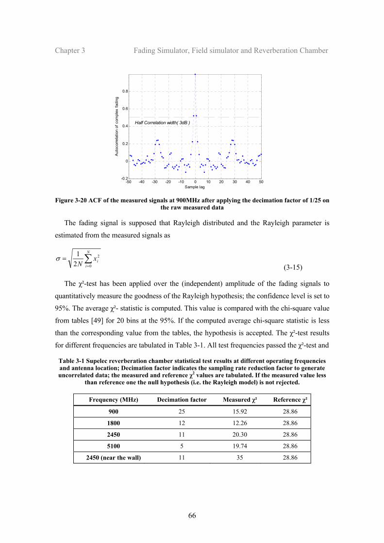
Chapter 3 Fading Simulator, Field simulator and Reverberation Chamber
66
-50 -40 -30 -20 -10 0 10 20 30 40 50-0.2
0
0.2
0.4
0.6
0.8
Sample lag
Aut
ocor
rela
tion
of c
ompl
ex fa
ding
Half Correlation width( 3dB )
Figure 3-20 ACF of the measured signals at 900MHz after applying the decimation factor of 1/25 on
the raw measured data
The fading signal is supposed that Rayleigh distributed and the Rayleigh parameter is
estimated from the measured signals as
∑=
=N
iix
N 0
2
21σ
(3-15)
The χ²-test has been applied over the (independent) amplitude of the fading signals to
quantitatively measure the goodness of the Rayleigh hypothesis; the confidence level is set to
95%. The average χ²- statistic is computed. This value is compared with the chi-square value
from tables [49] for 20 bins at the 95%. If the computed average chi-square statistic is less
than the corresponding value from the tables, the hypothesis is accepted. The χ²-test results
for different frequencies are tabulated in Table 3-1. All test frequencies passed the χ²-test and
Table 3-1 Supelec reverberation chamber statistical test results at different operating frequencies and antenna location; Decimation factor indicates the sampling rate reduction factor to generate uncorrelated data; the measured and reference χ2 values are tabulated. If the measured value less
than reference one the null hypothesis (i.e. the Rayleigh model) is not rejected.
Frequency (MHz) Decimation factor Measured χ² Reference χ²
900 25 15.92 28.86
1800 12 12.26 28.86
2450 11 20.30 28.86
5100 5 19.74 28.86
2450 (near the wall) 11 35 28.86
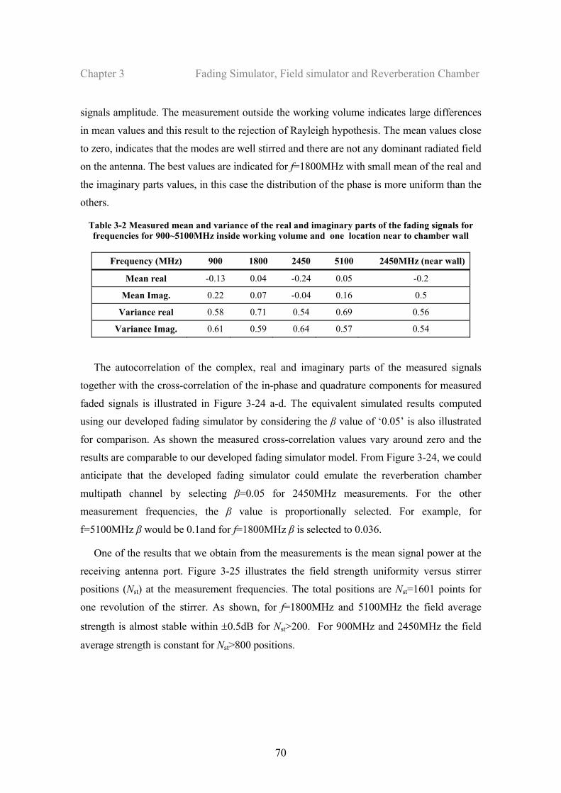
Chapter 3 Fading Simulator, Field simulator and Reverberation Chamber
70
signals amplitude. The measurement outside the working volume indicates large differences
in mean values and this result to the rejection of Rayleigh hypothesis. The mean values close
to zero, indicates that the modes are well stirred and there are not any dominant radiated field
on the antenna. The best values are indicated for f=1800MHz with small mean of the real and
the imaginary parts values, in this case the distribution of the phase is more uniform than the
others.
Table 3-2 Measured mean and variance of the real and imaginary parts of the fading signals for frequencies for 900~5100MHz inside working volume and one location near to chamber wall
Frequency (MHz) 900 1800 2450 5100 2450MHz (near wall)
Mean real -0.13 0.04 -0.24 0.05 -0.2
Mean Imag. 0.22 0.07 -0.04 0.16 0.5
Variance real 0.58 0.71 0.54 0.69 0.56
Variance Imag. 0.61 0.59 0.64 0.57 0.54
The autocorrelation of the complex, real and imaginary parts of the measured signals
together with the cross-correlation of the in-phase and quadrature components for measured
faded signals is illustrated in Figure 3-24 a-d. The equivalent simulated results computed
using our developed fading simulator by considering the β value of ‘0.05’ is also illustrated
for comparison. As shown the measured cross-correlation values vary around zero and the
results are comparable to our developed fading simulator model. From Figure 3-24, we could
anticipate that the developed fading simulator could emulate the reverberation chamber
multipath channel by selecting β=0.05 for 2450MHz measurements. For the other
measurement frequencies, the β value is proportionally selected. For example, for
f=5100MHz β would be 0.1and for f=1800MHz β is selected to 0.036.
One of the results that we obtain from the measurements is the mean signal power at the
receiving antenna port. Figure 3-25 illustrates the field strength uniformity versus stirrer
positions (Nst) at the measurement frequencies. The total positions are Nst=1601 points for
one revolution of the stirrer. As shown, for f=1800MHz and 5100MHz the field average
strength is almost stable within ±0.5dB for Nst>200. For 900MHz and 2450MHz the field
average strength is constant for Nst>800 positions.
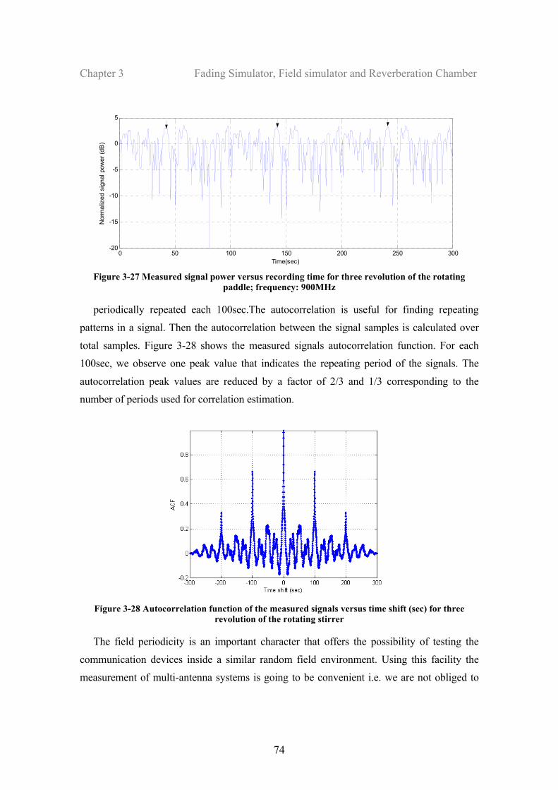
Chapter 3 Fading Simulator, Field simulator and Reverberation Chamber
74
0 50 100 150 200 250 300-20
-15
-10
-5
0
5
Nor
mal
ized
sig
nal p
ower
(dB
)
Time(sec) Figure 3-27 Measured signal power versus recording time for three revolution of the rotating
paddle; frequency: 900MHz
periodically repeated each 100sec.The autocorrelation is useful for finding repeating
patterns in a signal. Then the autocorrelation between the signal samples is calculated over
total samples. Figure 3-28 shows the measured signals autocorrelation function. For each
100sec, we observe one peak value that indicates the repeating period of the signals. The
autocorrelation peak values are reduced by a factor of 2/3 and 1/3 corresponding to the
number of periods used for correlation estimation.
Figure 3-28 Autocorrelation function of the measured signals versus time shift (sec) for three
revolution of the rotating stirrer
The field periodicity is an important character that offers the possibility of testing the
communication devices inside a similar random field environment. Using this facility the
measurement of multi-antenna systems is going to be convenient i.e. we are not obliged to
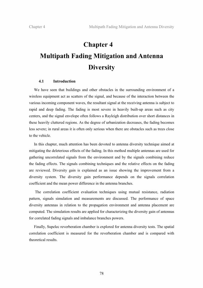
Chapter 4 Multipath Fading Mitigation and Antenna Diversity
78
Chapter 4
Multipath Fading Mitigation and Antenna
Diversity
4.1 Introduction
We have seen that buildings and other obstacles in the surrounding environment of a
wireless equipment act as scatters of the signal, and because of the interaction between the
various incoming component waves, the resultant signal at the receiving antenna is subject to
rapid and deep fading. The fading is most severe in heavily built-up areas such as city
centers, and the signal envelope often follows a Rayleigh distribution over short distances in
these heavily cluttered regions. As the degree of urbanization decreases, the fading becomes
less severe; in rural areas it is often only serious when there are obstacles such as trees close
to the vehicle.
In this chapter, much attention has been devoted to antenna diversity technique aimed at
mitigating the deleterious effects of the fading. In this method multiple antennas are used for
gathering uncorrelated signals from the environment and by the signals combining reduce
the fading effects. The signals combining techniques and the relative effects on the fading
are reviewed. Diversity gain is explained as an issue showing the improvement from a
diversity system. The diversity gain performance depends on the signals correlation
coefficient and the mean power difference in the antenna branches.
The correlation coefficient evaluation techniques using mutual resistance, radiation
pattern, signals simulation and measurements are discussed. The performance of space
diversity antennas in relation to the propagation environment and antenna placement are
computed. The simulation results are applied for characterizing the diversity gain of antennas
for correlated fading signals and imbalance branches powers.
Finally, Supelec reverberation chamber is explored for antenna diversity tests. The spatial
correlation coefficient is measured for the reverberation chamber and is compared with
theoretical results.
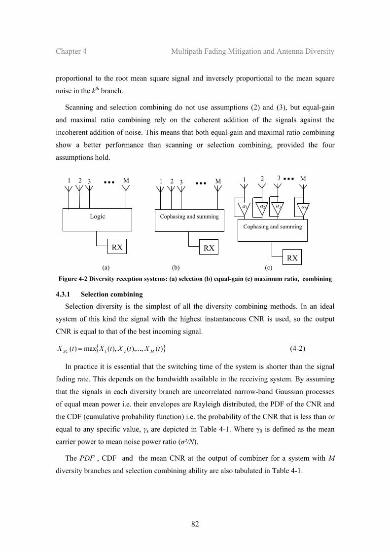
Chapter 4 Multipath Fading Mitigation and Antenna Diversity
82
proportional to the root mean square signal and inversely proportional to the mean square
noise in the kth branch.
Scanning and selection combining do not use assumptions (2) and (3), but equal-gain
and maximal ratio combining rely on the coherent addition of the signals against the
incoherent addition of noise. This means that both equal-gain and maximal ratio combining
show a better performance than scanning or selection combining, provided the four
assumptions hold.
(a) (b) (c)
Figure 4-2 Diversity reception systems: (a) selection (b) equal-gain (c) maximum ratio, combining
4.3.1 Selection combining
Selection diversity is the simplest of all the diversity combining methods. In an ideal
system of this kind the signal with the highest instantaneous CNR is used, so the output
CNR is equal to that of the best incoming signal.
)(),...,(),(max)( 21 tXtXtXtX MSC = (4-2)
In practice it is essential that the switching time of the system is shorter than the signal
fading rate. This depends on the bandwidth available in the receiving system. By assuming
that the signals in each diversity branch are uncorrelated narrow-band Gaussian processes
of equal mean power i.e. their envelopes are Rayleigh distributed, the PDF of the CNR and
the CDF (cumulative probability function) i.e. the probability of the CNR that is less than or
equal to any specific value, γs are depicted in Table 4-1. Where γ0 is defined as the mean
carrier power to mean noise power ratio (σ²/N).
The PDF , CDF and the mean CNR at the output of combiner for a system with M
diversity branches and selection combining ability are also tabulated in Table 4-1.
Logic
RX
1 2 3 M
Cophasing and summing
RX
1 2 3 M
Cophasing and summing
RX
1 2 3 M
a1 a2 a3 aM
Chapter 4 Multipath Fading Mitigation and Antenna Diversity
86
diversity is the ability to reduce the number of deep fades in the output signal. In statistical
terms, diversity changes the distribution of the output CNR and it no longer has an
exponential distribution. This cannot be achieved just by increasing the transmitter power.
To show this effect, the first-order envelope statistics of the signal, i.e. the way the signal
behaves as a function of time, Cumulative probability distributions of the composite signal
have been calculated for Rayleigh distributed individual branches with equal mean CNR
(γ0). For two-branch SC, EGC and MRC systems the appropriate cumulative distributions
are tabulated in Table 4-1. Figure 4-5 illustrates the CDF of these equations. The CDF of
Rayleigh is also illustrated for comparison showing the single branch distribution. It is clear
that the diversity curves are much flatter than the single-branch curve, indicating the lower
probability of fading.
-40 -35 -30 -25 -20 -15 -10 -5 0 5 1010-4
10-3
10-2
10-1
100
CNR
Cum
ulat
ive
prob
abili
ty
MRC EGC
SC Rayleigh
Figure 4-5 CDF plot of the output CNR for two-branch diversity system for SC, MRC and EGC
To gain a quantitative measure of the improvement, we note that the predicted reliability
for two-branch selection is 99% (0.01 CDF level) in circumstances where a single-branch
system would be only about 88% (0.12 CDF level) reliable. This means that the coverage
area of the transmitter is far and there are fewer areas in which signal flutter causes
problems. A comparable result can be achieved by alternating the CNR improvements in a
system with and without diversity application. The diversity gain is defined as the
increment in CNR in diversity system by comparison to a system without diversity and for a
defined CDF level. For instance in Figure 4-5, the transmitter power would involve an
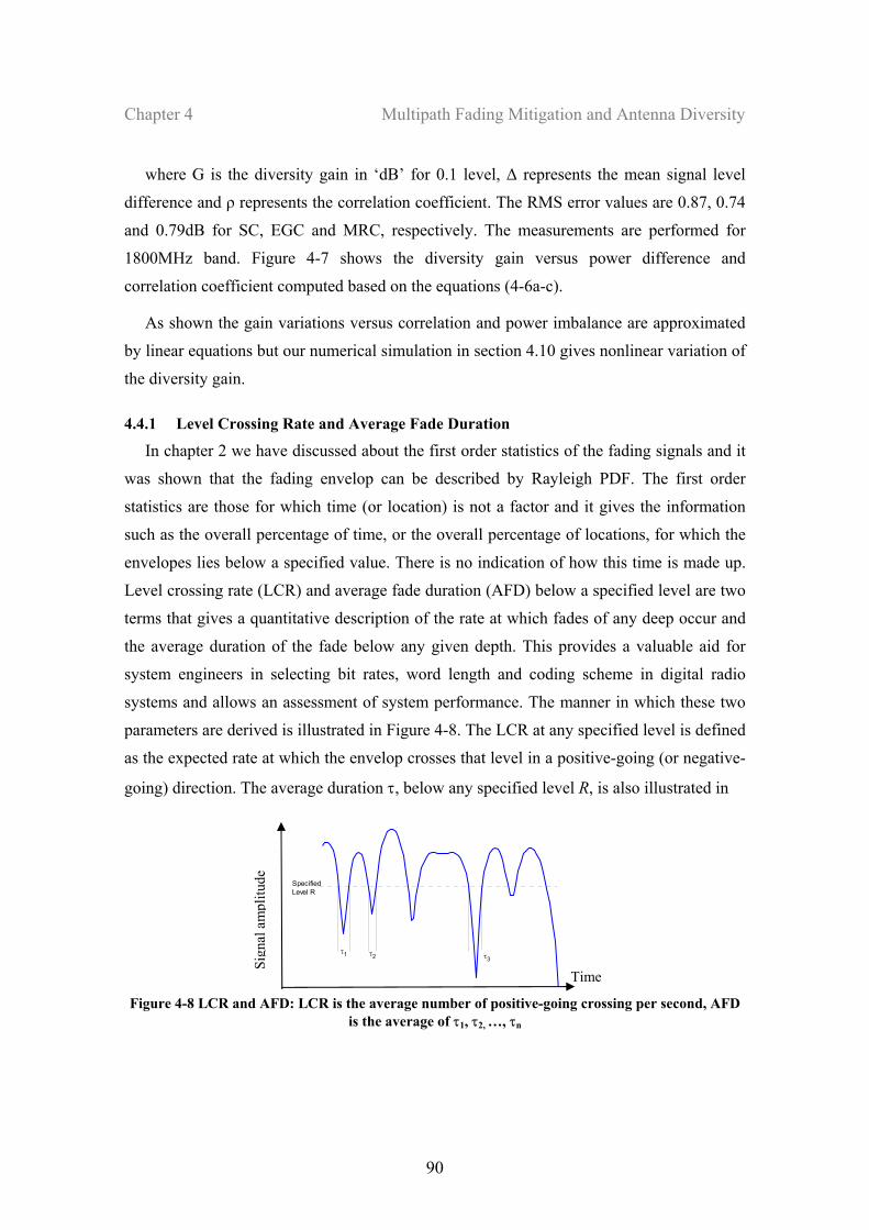
Chapter 4 Multipath Fading Mitigation and Antenna Diversity
90
where G is the diversity gain in ‘dB’ for 0.1 level, ∆ represents the mean signal level
difference and ρ represents the correlation coefficient. The RMS error values are 0.87, 0.74
and 0.79dB for SC, EGC and MRC, respectively. The measurements are performed for
1800MHz band. Figure 4-7 shows the diversity gain versus power difference and
correlation coefficient computed based on the equations (4-6a-c).
As shown the gain variations versus correlation and power imbalance are approximated
by linear equations but our numerical simulation in section 4.10 gives nonlinear variation of
the diversity gain.
4.4.1 Level Crossing Rate and Average Fade Duration
In chapter 2 we have discussed about the first order statistics of the fading signals and it
was shown that the fading envelop can be described by Rayleigh PDF. The first order
statistics are those for which time (or location) is not a factor and it gives the information
such as the overall percentage of time, or the overall percentage of locations, for which the
envelopes lies below a specified value. There is no indication of how this time is made up.
Level crossing rate (LCR) and average fade duration (AFD) below a specified level are two
terms that gives a quantitative description of the rate at which fades of any deep occur and
the average duration of the fade below any given depth. This provides a valuable aid for
system engineers in selecting bit rates, word length and coding scheme in digital radio
systems and allows an assessment of system performance. The manner in which these two
parameters are derived is illustrated in Figure 4-8. The LCR at any specified level is defined
as the expected rate at which the envelop crosses that level in a positive-going (or negative-
going) direction. The average duration τ, below any specified level R, is also illustrated in
τ1 τ2 τ3
SpecifiedLevel R
Figure 4-8 LCR and AFD: LCR is the average number of positive-going crossing per second, AFD
is the average of τ1, τ2, …, τn
Time Sig
nal a
mpl
itude
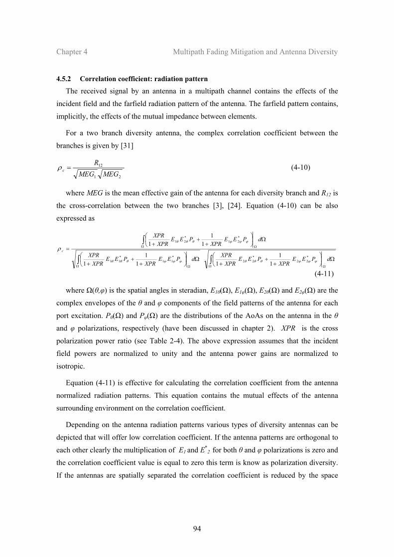
Chapter 4 Multipath Fading Mitigation and Antenna Diversity
94
4.5.2 Correlation coefficient: radiation pattern
The received signal by an antenna in a multipath channel contains the effects of the
incident field and the farfield radiation pattern of the antenna. The farfield pattern contains,
implicitly, the effects of the mutual impedance between elements.
For a two branch diversity antenna, the complex correlation coefficient between the
branches is given by [31]
21
12
MEGMEGR
c =ρ (4-10)
where MEG is the mean effective gain of the antenna for each diversity branch and R12 is
the cross-correlation between the two branches [3], [24]. Equation (4-10) can be also
expressed as
∫∫
∫
Ω ΩΩ Ω
Ω Ω
Ω⎟⎠⎞
⎜⎝⎛
++
+Ω⎟
⎠⎞
⎜⎝⎛
++
+
Ω⎟⎠⎞
⎜⎝⎛
++
+=
dPEEXPR
PEEXPR
XPRdPEEXPR
PEEXPR
XPR
dPEEXPR
PEEXPR
XPR
c
ϕϕϕθθθϕϕϕθθθ
ϕϕϕθθθ
ρ*22
*22
*11
*11
*21
*21
11
111
1
11
1
(4-11)
where Ω(θ,φ) is the spatial angles in steradian, E1θ(Ω), E1φ(Ω), E2θ(Ω) and E2φ(Ω) are the
complex envelopes of the θ and φ components of the field patterns of the antenna for each
port excitation. Pθ(Ω) and Pφ(Ω) are the distributions of the AoAs on the antenna in the θ
and φ polarizations, respectively (have been discussed in chapter 2). XPR is the cross
polarization power ratio (see Table 2-4). The above expression assumes that the incident
field powers are normalized to unity and the antenna power gains are normalized to
isotropic.
Equation (4-11) is effective for calculating the correlation coefficient from the antenna
normalized radiation patterns. This equation contains the mutual effects of the antenna
surrounding environment on the correlation coefficient.
Depending on the antenna radiation patterns various types of diversity antennas can be
depicted that will offer low correlation coefficient. If the antenna patterns are orthogonal to
each other clearly the multiplication of E1 and E*2 for both θ and φ polarizations is zero and
the correlation coefficient value is equal to zero this term is know as polarization diversity.
If the antennas are spatially separated the correlation coefficient is reduced by the space
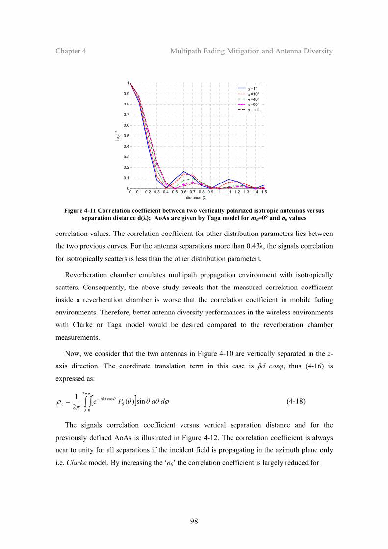
Chapter 4 Multipath Fading Mitigation and Antenna Diversity
98
0 0.1 0.2 0.3 0.4 0.5 0.6 0.7 0.8 0.9 1 1.1 1.2 1.3 1.4 1.50
0.1
0.2
0.3
0.4
0.5
0.6
0.7
0.8
0.9
1
distance (λ)
| ρc| ²
σ=1°σ=10°σ=40°σ=90°σ= inf
Figure 4-11 Correlation coefficient between two vertically polarized isotropic antennas versus
separation distance d(λ); AoAs are given by Taga model for mθ=0° and σθ values
correlation values. The correlation coefficient for other distribution parameters lies between
the two previous curves. For the antenna separations more than 0.43λ, the signals correlation
for isotropically scatters is less than the other distribution parameters.
Reverberation chamber emulates multipath propagation environment with isotropically
scatters. Consequently, the above study reveals that the measured correlation coefficient
inside a reverberation chamber is worse that the correlation coefficient in mobile fading
environments. Therefore, better antenna diversity performances in the wireless environments
with Clarke or Taga model would be desired compared to the reverberation chamber
measurements.
Now, we consider that the two antennas in Figure 4-10 are vertically separated in the z-
axis direction. The coordinate translation term in this case is βd cosφ, thus (4-16) is
expressed as:
[ ] ϕθθθπ
ρπ π
θθβ ddPe dj
c sin)(21 2
0 0
cos∫ ∫ −= (4-18)
The signals correlation coefficient versus vertical separation distance and for the
previously defined AoAs is illustrated in Figure 4-12. The correlation coefficient is always
near to unity for all separations if the incident field is propagating in the azimuth plane only
i.e. Clarke model. By increasing the ‘σθ’ the correlation coefficient is largely reduced for
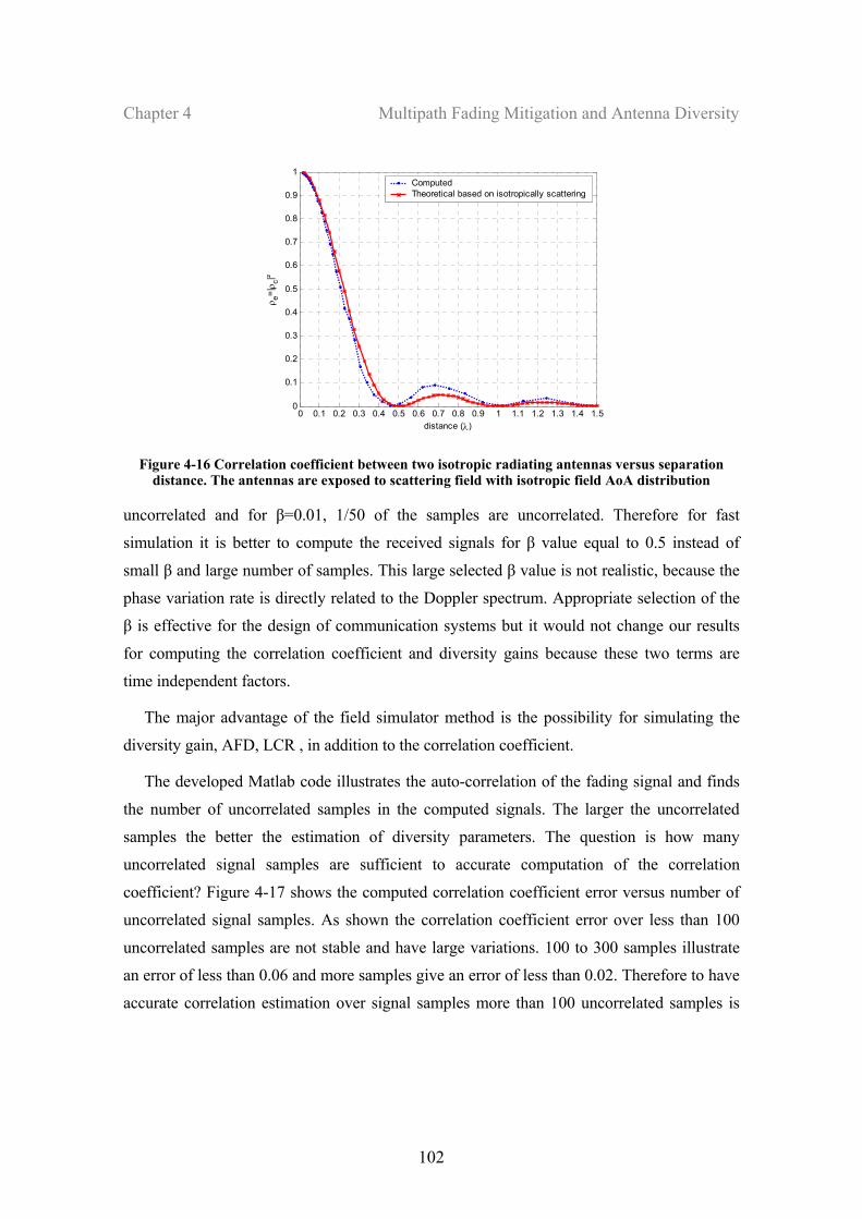
Chapter 4 Multipath Fading Mitigation and Antenna Diversity
102
0 0.1 0.2 0.3 0.4 0.5 0.6 0.7 0.8 0.9 1 1.1 1.2 1.3 1.4 1.50
0.1
0.2
0.3
0.4
0.5
0.6
0.7
0.8
0.9
1
distance (λ)
ρ e=|ρ c|²
ComputedTheoretical based on isotropically scattering
Figure 4-16 Correlation coefficient between two isotropic radiating antennas versus separation distance. The antennas are exposed to scattering field with isotropic field AoA distribution
uncorrelated and for β=0.01, 1/50 of the samples are uncorrelated. Therefore for fast
simulation it is better to compute the received signals for β value equal to 0.5 instead of
small β and large number of samples. This large selected β value is not realistic, because the
phase variation rate is directly related to the Doppler spectrum. Appropriate selection of the
β is effective for the design of communication systems but it would not change our results
for computing the correlation coefficient and diversity gains because these two terms are
time independent factors.
The major advantage of the field simulator method is the possibility for simulating the
diversity gain, AFD, LCR , in addition to the correlation coefficient.
The developed Matlab code illustrates the auto-correlation of the fading signal and finds
the number of uncorrelated samples in the computed signals. The larger the uncorrelated
samples the better the estimation of diversity parameters. The question is how many
uncorrelated signal samples are sufficient to accurate computation of the correlation
coefficient? Figure 4-17 shows the computed correlation coefficient error versus number of
uncorrelated signal samples. As shown the correlation coefficient error over less than 100
uncorrelated samples are not stable and have large variations. 100 to 300 samples illustrate
an error of less than 0.06 and more samples give an error of less than 0.02. Therefore to have
accurate correlation estimation over signal samples more than 100 uncorrelated samples is
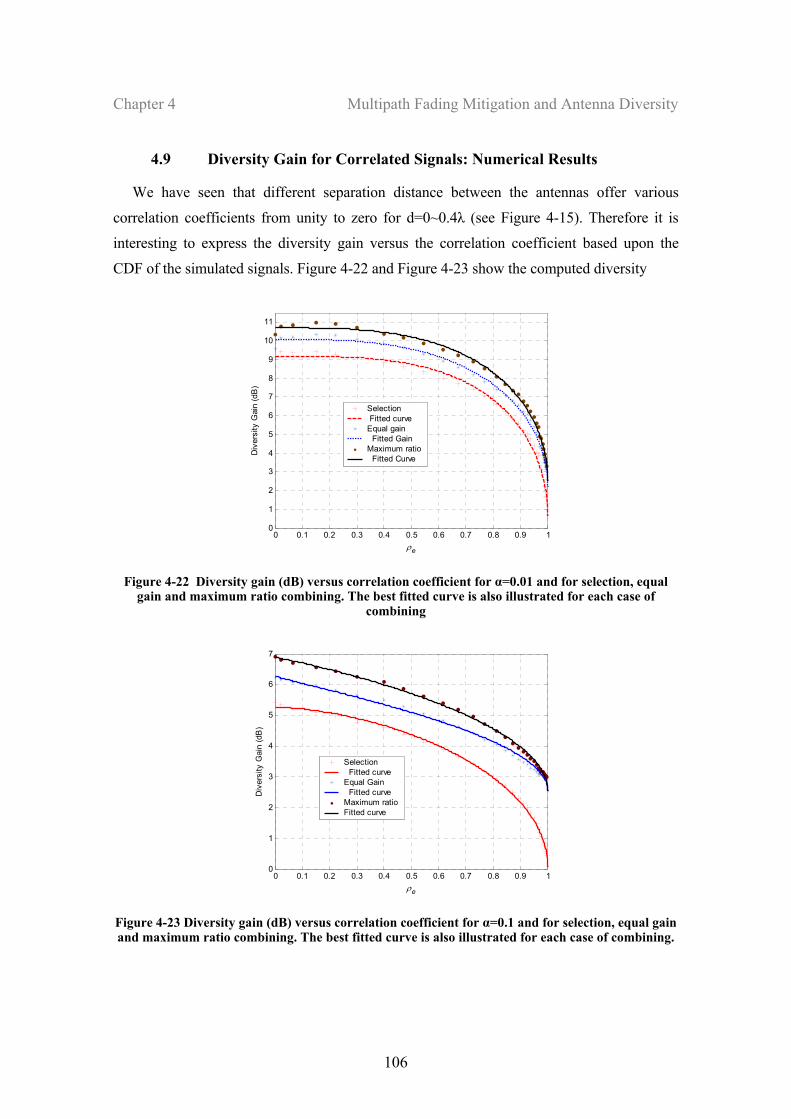
Chapter 4 Multipath Fading Mitigation and Antenna Diversity
106
4.9 Diversity Gain for Correlated Signals: Numerical Results
We have seen that different separation distance between the antennas offer various
correlation coefficients from unity to zero for d=0~0.4λ (see Figure 4-15). Therefore it is
interesting to express the diversity gain versus the correlation coefficient based upon the
CDF of the simulated signals. Figure 4-22 and Figure 4-23 show the computed diversity
0 0.1 0.2 0.3 0.4 0.5 0.6 0.7 0.8 0.9 10
1
2
3
4
5
6
7
8
9
10
11
ρe
Div
ersi
ty G
ain
(dB
)
Selection Fitted curveEqual gain Fitted GainMaximum ratio Fitted Curve
Figure 4-22 Diversity gain (dB) versus correlation coefficient for α=0.01 and for selection, equal gain and maximum ratio combining. The best fitted curve is also illustrated for each case of
combining
0 0.1 0.2 0.3 0.4 0.5 0.6 0.7 0.8 0.9 10
1
2
3
4
5
6
7
ρe
Div
ersi
ty G
ain
(dB
)
Selection Fitted curveEqual Gain Fitted curveMaximum ratioFitted curve
Figure 4-23 Diversity gain (dB) versus correlation coefficient for α=0.1 and for selection, equal gain and maximum ratio combining. The best fitted curve is also illustrated for each case of combining.
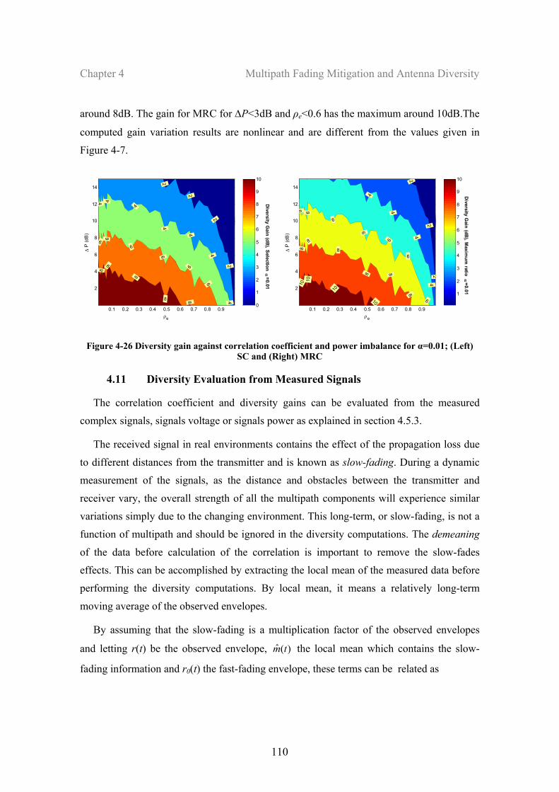
Chapter 4 Multipath Fading Mitigation and Antenna Diversity
110
around 8dB. The gain for MRC for ∆P<3dB and ρe<0.6 has the maximum around 10dB.The
computed gain variation results are nonlinear and are different from the values given in
Figure 4-7.
0.1 0.2 0.3 0.4 0.5 0.6 0.7 0.8 0.9
2
4
6
8
10
12
14
ρe
∆ P
(dB
)
2
2
2
2
4 4
4
4
4
4
4
6 6
6
6
6
6
8
8
8
8 8
0
1
2
3
4
5
6
7
8
9
10
Diversity G
ain (dB), S
election α=0.01
0.1 0.2 0.3 0.4 0.5 0.6 0.7 0.8 0.9
2
4
6
8
10
12
14
ρe
∆ P
(dB
)
2
22
4
4
4
4
6
6
6
6
6
6
68
8
8
8 8
8
1010
10
10
1
2
3
4
5
6
7
8
9
10
Diversity G
ain (dB), M
aximum
ratio α =0.01
Figure 4-26 Diversity gain against correlation coefficient and power imbalance for α=0.01; (Left) SC and (Right) MRC
4.11 Diversity Evaluation from Measured Signals
The correlation coefficient and diversity gains can be evaluated from the measured
complex signals, signals voltage or signals power as explained in section 4.5.3.
The received signal in real environments contains the effect of the propagation loss due
to different distances from the transmitter and is known as slow-fading. During a dynamic
measurement of the signals, as the distance and obstacles between the transmitter and
receiver vary, the overall strength of all the multipath components will experience similar
variations simply due to the changing environment. This long-term, or slow-fading, is not a
function of multipath and should be ignored in the diversity computations. The demeaning
of the data before calculation of the correlation is important to remove the slow-fades
effects. This can be accomplished by extracting the local mean of the measured data before
performing the diversity computations. By local mean, it means a relatively long-term
moving average of the observed envelopes.
By assuming that the slow-fading is a multiplication factor of the observed envelopes
and letting r(t) be the observed envelope, )(ˆ tm the local mean which contains the slow-
fading information and r0(t) the fast-fading envelope, these terms can be related as
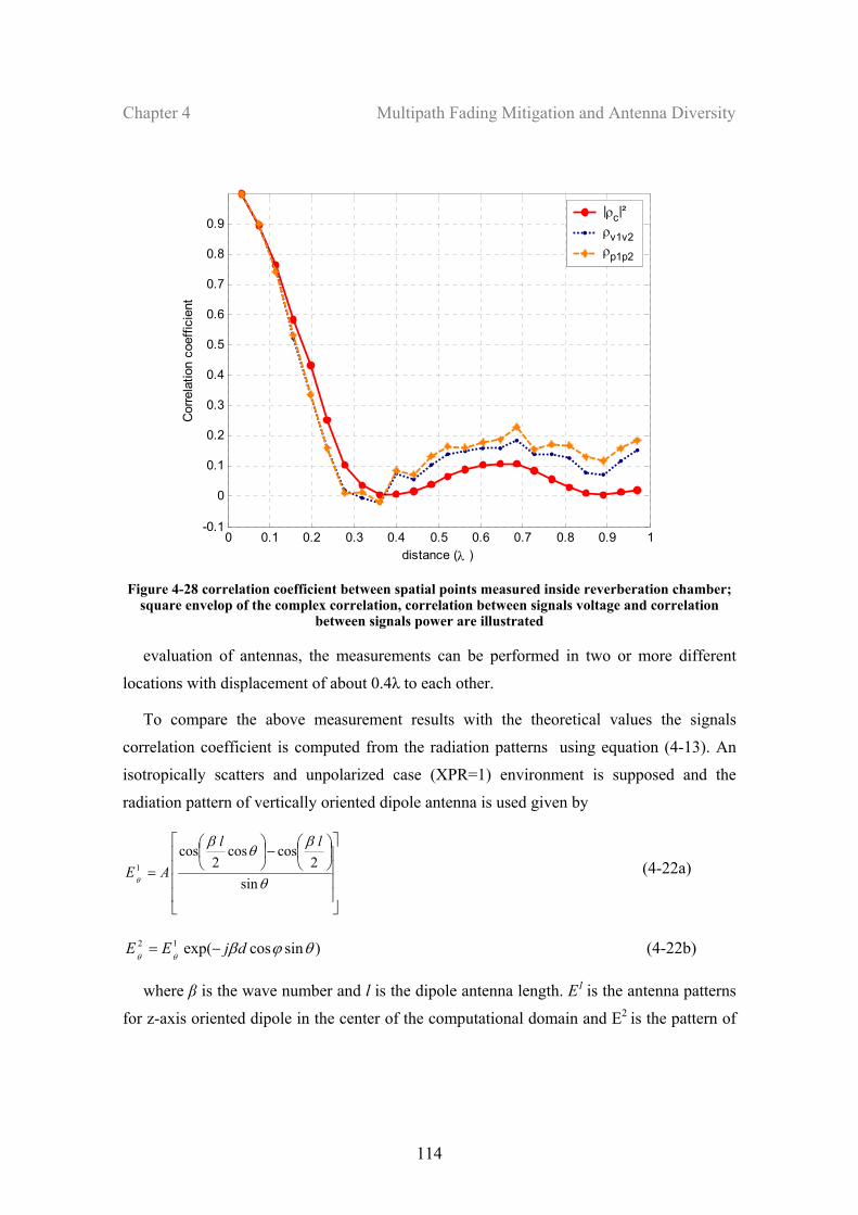
Chapter 4 Multipath Fading Mitigation and Antenna Diversity
114
0 0.1 0.2 0.3 0.4 0.5 0.6 0.7 0.8 0.9 1-0.1
0
0.1
0.2
0.3
0.4
0.5
0.6
0.7
0.8
0.9
distance (λ )
Cor
rela
tion
coef
ficie
nt
|ρc|²ρv1v2ρp1p2
Figure 4-28 correlation coefficient between spatial points measured inside reverberation chamber;
square envelop of the complex correlation, correlation between signals voltage and correlation between signals power are illustrated
evaluation of antennas, the measurements can be performed in two or more different
locations with displacement of about 0.4λ to each other.
To compare the above measurement results with the theoretical values the signals
correlation coefficient is computed from the radiation patterns using equation (4-13). An
isotropically scatters and unpolarized case (XPR=1) environment is supposed and the
radiation pattern of vertically oriented dipole antenna is used given by
⎥⎥⎥⎥
⎦
⎤
⎢⎢⎢⎢
⎣
⎡⎟⎠
⎞⎜⎝
⎛−⎟⎠
⎞⎜⎝
⎛
=θ
βθ
β
θ sin2
coscos2
cos1
ll
AE (4-22a)
)sincosexp(12 θϕβθθ
djEE −= (4-22b)
where β is the wave number and l is the dipole antenna length. E1 is the antenna patterns
for z-axis oriented dipole in the center of the computational domain and E2 is the pattern of
Chapter 4 Multipath Fading Mitigation and Antenna Diversity
118
imbalanced and the branch signals are correlated the system performance is mitigated. The
diversity gain variation curves for the present condition are computed.
Diversity performance can be evaluated by direct measurements in multipath fading
channels. The measured signals must be processed to eliminate the slow fading effects; the
data demeaning is a technique in this approach. Reverberation chamber based measurement
does not require the data demeaning due to the fact that the distance between the transmitting
antenna and the receiving antenna is constant.
Signal sounding in Supelec reverberation chamber is conducted to evaluate the
correlation between spatial locations in the chamber. An especial setup is used to measure
the correlation coefficient variations. Envelop, voltage and power correlations versus
distance are measured. The measured decorrelation distance inside the reverberation
chamber is 0.4λ; this specifies the effective spatial displacement for gathering large number
of uncorrelated signal samples. LCR and AFD curves are measured in the MSRC and are
compared with the theoretical curves given for mobile multipath channels. Good accordance
is resulted.
Chapter 5 Antenna Diversity for Mobile phone Communication
122
It is also shown that the patterns can have very similar shapes and still be uncorrelated if the
patterns phases are different.
The simulations are followed by laboratory measurements carried out in Supelec
reverberation chamber. The measurements are performed at 2450MHz with two standard
(half-wave) dipole antennas; the signals correlation coefficient is precisely measured with
high resolution of the antenna distances, has not been performed before [67]. The selected
high frequency and the large chamber size increase the measurement accuracy.
Diversity gain for SC and MRC versus dipoles separations are computed from the
measured signals. Effective diversity gain which represents the gain over a single antenna
and includes the influence of correlation coefficient and mean effective gain is measured.
The mean received power degradation at the coupled antennas is measured and is compared
with the modeled antenna radiation efficiency.
5.2.1 Signals Correlation coefficient: radiation pattern
The signals correlation coefficient between two antenna patterns in an isotropically
scattering field environment and unpolarized case ( XPR=1 ) is given by equation (4-13).
This model of the field scatters corresponds to the reverberation chamber multipath or
equally indoor environment where there are many nearby scatters [70]. If the antennas are
vertically polarized, as is the case in parallel side-by-side and z-oriented dipoles (E1φ=
E2φ=0), equation (4-13) is simplified to
( ) ( ) ( ) ( )∫∫Ω
ΩΨ
Ω
∗ ΩΩ=ΩΩΩ= deCdEE jc ππ
ρ θθ 41.
41
21 (5-1)
Equation (5.1) is expressed as a function of the pattern-coupling magnitude and pattern-
coupling phase factors, |C(Ω)| and Ψ(Ω), respectively. The signals envelop correlation
coefficient is related to the complex correlation (5-1) by the equation (4-7).
The correlation coefficient between two identical patterns which are circularly symmetric
and horizontally separated with distance ‘d’ is given by the zero order Bessel function J0(βd),
where β is the wave number. This is so called Clarke function and shows the space diversity
effects [51].
The correlation coefficient between two half-wave dipoles Figure 5-2, which are parallel,
z-oriented and horizontally separated with distance d, can be computed from the dipole
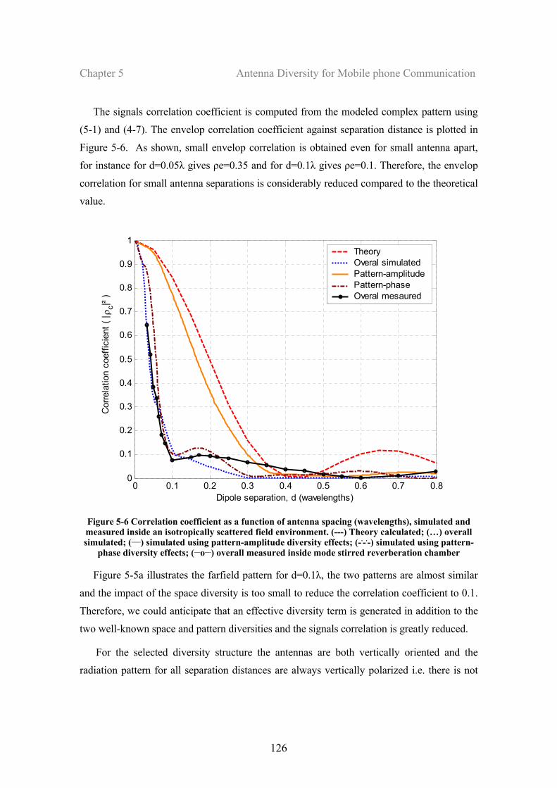
Chapter 5 Antenna Diversity for Mobile phone Communication
126
The signals correlation coefficient is computed from the modeled complex pattern using
(5-1) and (4-7). The envelop correlation coefficient against separation distance is plotted in
Figure 5-6. As shown, small envelop correlation is obtained even for small antenna apart,
for instance for d=0.05λ gives ρe=0.35 and for d=0.1λ gives ρe=0.1. Therefore, the envelop
correlation for small antenna separations is considerably reduced compared to the theoretical
value.
0 0.1 0.2 0.3 0.4 0.5 0.6 0.7 0.80
0.1
0.2
0.3
0.4
0.5
0.6
0.7
0.8
0.9
1
Dipole separation, d (wavelengths)
TheoryOveral simulatedPattern-amplitudePattern-phaseOveral mesaured
Cor
rela
tion
coef
ficie
nt (
| ρc|²
)
Figure 5-6 Correlation coefficient as a function of antenna spacing (wavelengths), simulated and measured inside an isotropically scattered field environment. (---) Theory calculated; (…) overall simulated; (___) simulated using pattern-amplitude diversity effects; (-.-.-) simulated using pattern-
phase diversity effects; (__o__) overall measured inside mode stirred reverberation chamber
Figure 5-5a illustrates the farfield pattern for d=0.1λ, the two patterns are almost similar
and the impact of the space diversity is too small to reduce the correlation coefficient to 0.1.
Therefore, we could anticipate that an effective diversity term is generated in addition to the
two well-known space and pattern diversities and the signals correlation is greatly reduced.
For the selected diversity structure the antennas are both vertically oriented and the
radiation pattern for all separation distances are always vertically polarized i.e. there is not
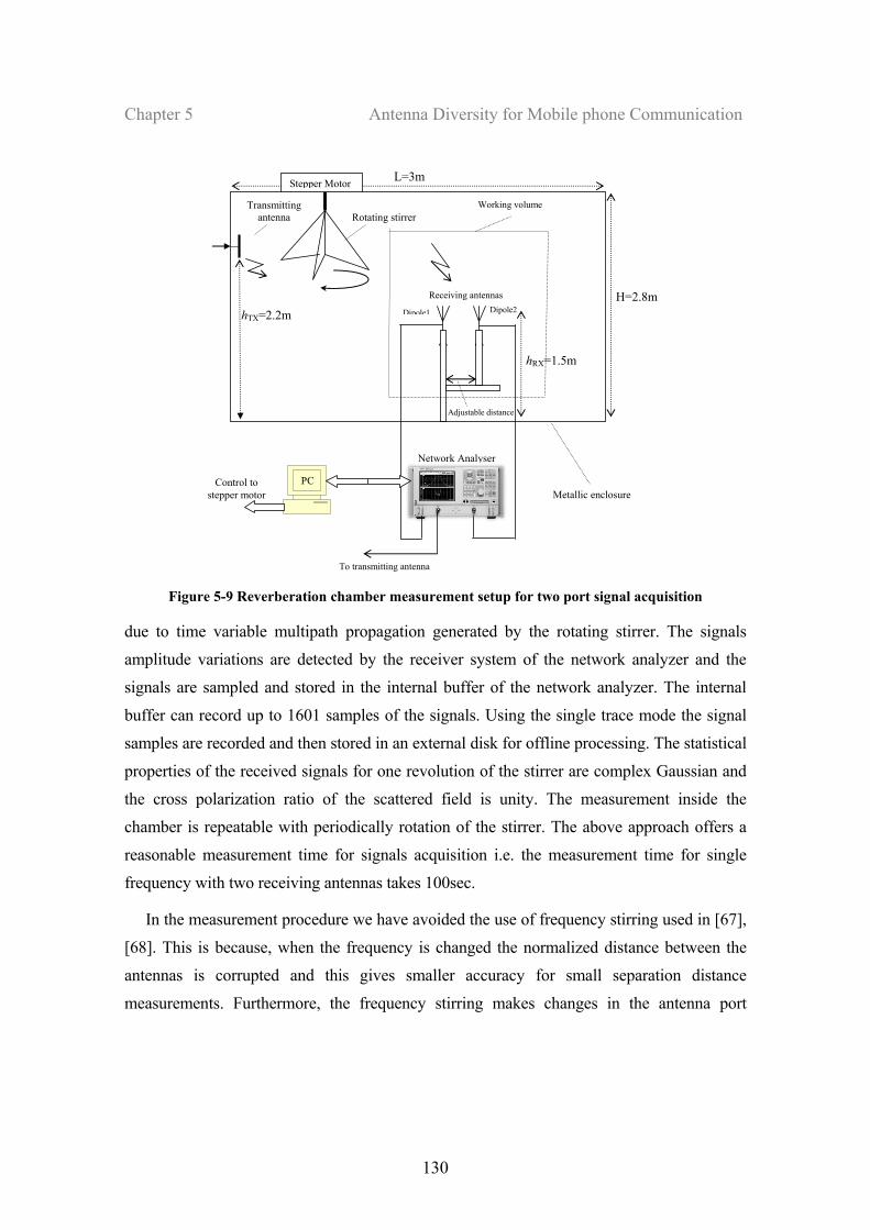
Chapter 5 Antenna Diversity for Mobile phone Communication
130
Stepper Motor
Transmitting antenna
PC
Network Analyser
Rotating stirrer
Control to stepper motor
Dipole1 Dipole2
To transmitting antenna
hTX=2.2m H=2.8m
L=3m
hRX=1.5m
Adjustable distance
Receiving antennas
Working volume
Metallic enclosure
Figure 5-9 Reverberation chamber measurement setup for two port signal acquisition
due to time variable multipath propagation generated by the rotating stirrer. The signals
amplitude variations are detected by the receiver system of the network analyzer and the
signals are sampled and stored in the internal buffer of the network analyzer. The internal
buffer can record up to 1601 samples of the signals. Using the single trace mode the signal
samples are recorded and then stored in an external disk for offline processing. The statistical
properties of the received signals for one revolution of the stirrer are complex Gaussian and
the cross polarization ratio of the scattered field is unity. The measurement inside the
chamber is repeatable with periodically rotation of the stirrer. The above approach offers a
reasonable measurement time for signals acquisition i.e. the measurement time for single
frequency with two receiving antennas takes 100sec.
In the measurement procedure we have avoided the use of frequency stirring used in [67],
[68]. This is because, when the frequency is changed the normalized distance between the
antennas is corrupted and this gives smaller accuracy for small separation distance
measurements. Furthermore, the frequency stirring makes changes in the antenna port
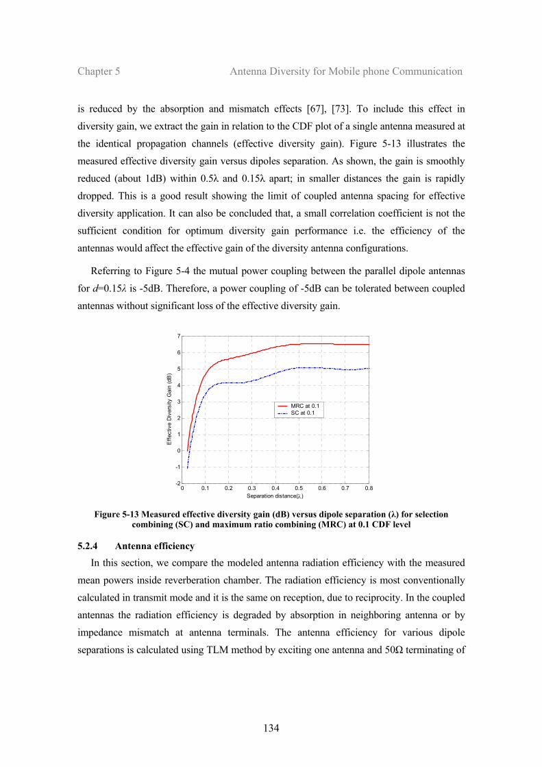
Chapter 5 Antenna Diversity for Mobile phone Communication
134
is reduced by the absorption and mismatch effects [67], [73]. To include this effect in
diversity gain, we extract the gain in relation to the CDF plot of a single antenna measured at
the identical propagation channels (effective diversity gain). Figure 5-13 illustrates the
measured effective diversity gain versus dipoles separation. As shown, the gain is smoothly
reduced (about 1dB) within 0.5λ and 0.15λ apart; in smaller distances the gain is rapidly
dropped. This is a good result showing the limit of coupled antenna spacing for effective
diversity application. It can also be concluded that, a small correlation coefficient is not the
sufficient condition for optimum diversity gain performance i.e. the efficiency of the
antennas would affect the effective gain of the diversity antenna configurations.
Referring to Figure 5-4 the mutual power coupling between the parallel dipole antennas
for d=0.15λ is -5dB. Therefore, a power coupling of -5dB can be tolerated between coupled
antennas without significant loss of the effective diversity gain.
0 0.1 0.2 0.3 0.4 0.5 0.6 0.7 0.8-2
-1
0
1
2
3
4
5
6
7
Separation distance(λ)
Effe
ctiv
e D
iver
sity
Gai
n (d
B)
MRC at 0.1SC at 0.1
Figure 5-13 Measured effective diversity gain (dB) versus dipole separation (λ) for selection
combining (SC) and maximum ratio combining (MRC) at 0.1 CDF level
5.2.4 Antenna efficiency
In this section, we compare the modeled antenna radiation efficiency with the measured
mean powers inside reverberation chamber. The radiation efficiency is most conventionally
calculated in transmit mode and it is the same on reception, due to reciprocity. In the coupled
antennas the radiation efficiency is degraded by absorption in neighboring antenna or by
impedance mismatch at antenna terminals. The antenna efficiency for various dipole
separations is calculated using TLM method by exciting one antenna and 50Ω terminating of
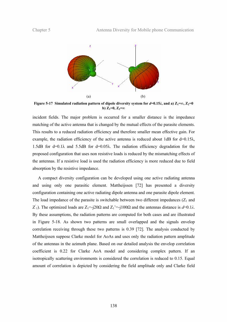
Chapter 5 Antenna Diversity for Mobile phone Communication
138
(a) (b)
Figure 5-17 Simulated radiation pattern of dipole diversity system for d=0.15λ, and a) Z1=∞, Z2=0 b) Z1=0, Z2=∞
incident fields. The major problem is occurred for a smaller distance is the impedance
matching of the active antenna that is changed by the mutual effects of the parasite elements.
This results to a reduced radiation efficiency and therefore smaller mean effective gain. For
example, the radiation efficiency of the active antenna is reduced about 1dB for d=0.15λ,
1.5dB for d=0.1λ and 5.5dB for d=0.05λ. The radiation efficiency degradation for the
proposed configuration that uses non resistive loads is reduced by the mismatching effects of
the antennas. If a resistive load is used the radiation efficiency is more reduced due to field
absorption by the resistive impedance.
A compact diversity configuration can be developed using one active radiating antenna
and using only one parasitic element. Mattheijssen [72] has presented a diversity
configuration containing one active radiating dipole antenna and one parasite dipole element.
The load impedance of the parasite is switchable between two different impedances (Z1 and
Z’1). The optimized loads are Z1=-j20Ω and Z1’=-j100Ω and the antennas distance is d=0.1λ.
By these assumptions, the radiation patterns are computed for both cases and are illustrated
in Figure 5-18. As shown two patterns are small overlapped and the signals envelop
correlation receiving through these two patterns is 0.39 [72]. The analysis conducted by
Mattheijssen suppose Clarke model for AoAs and uses only the radiation pattern amplitude
of the antennas in the azimuth plane. Based on our detailed analysis the envelop correlation
coefficient is 0.22 for Clarke AoA model and considering complex pattern. If an
isotropically scattering environments is considered the correlation is reduced to 0.15. Equal
amount of correlation is depicted by considering the field amplitude only and Clarke field
Chapter 5 Antenna Diversity for Mobile phone Communication
142
are obtained using wire model available by the package. The dimensions of the grids around
the wire model of the helical antennas are manually small selected (0.5mm in both x and y
directions and 0.25mm in z direction), therefore the helical antenna would be precisely
constructed after the model discretising. The total number of realized cells after meshing was
93104 and the allocated memory was 15M. The computation time using normal P4 with
512M RAM takes 12 minutes for two ports simulations.
The return loss in diversity branches and the mutual coupling of the constructed prototype
are experimentally measured using a calibrated network analyzer. The return loss
measurements are performed in a condition in which one antenna is connected to the
network and the next one is terminated to 50Ω load impedance. The measurement results are
different from single port antenna measurement because the induced current on the non-
excited antenna would change the current distributions along the exited element; therefore
the port impedance would be modified.
It is notable that the commercial helical antenna uses one helical turn around a metallic
core at the beginning of the helix for impedance matching, the plastic material are used as
the helical antenna core and the antenna is coated with plastic material. In the simulations
procedure we have not considered these options. The measured return-loss of the Sagem
helical antenna illustrates two resonance frequencies on 1010MHz and 1970MHz. These
frequencies are out of the GSM and DCS bands. To apply the antennas in the mobile
frequency bands we have coated the two antennas with additional isotherm plastic materials
therefore the two resonance frequencies are moved down to GSM/DCS bands.
The measured and simulated return loss for the antenna ports are given in Figure 5-21.
The simulated return loss for the second resonance frequency is small different from the
measurements. The impedance matching of the simulated model is worse than the
measurements, this issue results to smaller radiation efficiency of the simulated pattern.
The mutual power coupling (S21) between antenna ports is measured when one antenna is
transmitting and the other antenna is receiving. As shown in section 5.2 the mutual power
coupling has negative effects on the radiation efficiency but illustrate positive effects on the
signals correlation coefficient for diversity configurations. The measured and the simulated
mutual coupling versus frequency are illustrated in Figure 5-21. The antenna prototype is
symmetric, therefore similar results are observed for both antennas.
Chapter 5 Antenna Diversity for Mobile phone Communication
146
5.4.4 Signals correlation coefficient: mutual impedance
In section 4.5.1 it has been shown that the signals correlation coefficient can be
approximated by the normalized mutual resistance. To evaluate the mutual resistance the
complex scattering parameters of the antenna array are measured then, the conversion of S-
parameters to Z-parameters is performed. The approach is different from the direct
measurement of the Z-parameters using the network analyzer in the Smith chart operating
mode. This is because, the measured mutual impedance contains the effects of the self-
impedance that should be removed from the measurements.
The measured port impedance for 938MHz is Z11=47.5-j 2.6 and the mutual impedance is
37.6+ j4.1; this gives the normalized mutual resistance r12=0.79 and consequently envelop
correlation of ρe=0.62. For 1830MHz the port impedance is Z11=41.7 +j14.7 and the mutual
impedance is 19 +j12.8; this results the normalized resistance r12=0.45 and consequently
ρe=0.2.
The signals correlation coefficient is evaluated using radiation pattern and random field
measurement in the following sections. It has been shown that the given correlation
coefficient is considerably different from the mutual impedance approach.
5.4.5 Signals correlation coefficient for GSM band: pattern approach
Signals correlation coefficient is computed by the direct method (equation (4-11)) and
applying the antenna patterns and the field AoA models. The AoA models are given in Table
2-3 and the cross polarization ratio of the scattered field is supposed to be unity (XPR=1) for
all models.
For the GSM band the signals correlation coefficient is computed using the simulated and
the measured antenna patterns. Table 5-1 and Table 5-2 show the complex correlation
coefficient and the envelop correlation coefficient for various field scattering models. The
AoAs are specified with M0 corresponds to the model with isotropically scatters; M1 is
related to Clarke model with uniform scatters in the azimuth plane only; M2-1 and M2-2 are
supposed Gaussian distribution in the elevation and uniform in the azimuth (index 1 and 2
are related to Taga model parameters); M3 considers double-exponential distribution in the
elevation and uniform scatters in the azimuth (the double exponential parameters are given in
Table 2-3, we have selected the average of all environment (see Table 2-2) to construct the
double exponential model. The last model M4 corresponds to the elliptical model for the
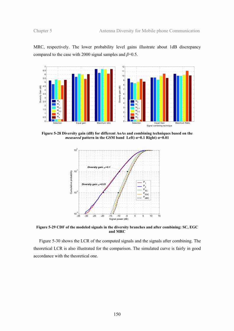
Chapter 5 Antenna Diversity for Mobile phone Communication
150
MRC, respectively. The lower probability level gains illustrate about 1dB discrepancy
compared to the case with 2000 signal samples and β=0.5.
Selection Equal gain Maximum ratio 0
0.5
1
1.5
2
2.5
3
3.5
4
4.5
5
5.5
6
6.5
7
Div
ersi
ty G
ain
(dB
)
M0M1M2-1M2-2M3M4
Selection Equal Gain Maximum Ratio0
1
2
3
4
5
6
7
8
9
10
11
12
Signal combining technique
Div
ersi
ty g
ain
(dB
)
M0M1M2-1M2-2M3M4
Figure 5-28 Diversity gain (dB) for different AoAs and combining techniques based on the
measured pattern in the GSM band Left) α=0.1 Right) α=0.01
-35 -30 -25 -20 -15 -10 -5 0 5 10 1510-3
10-2
10-1
100
Cum
ulat
ive
prob
abili
ty
Signal power (dB)
P1P2PSCPEGCPMRC
Diversity gain α=0.1
Diversity gain α=0.01
Figure 5-29 CDF of the modeled signals in the diversity branches and after combining: SC, EGC
and MRC
Figure 5-30 shows the LCR of the computed signals and the signals after combining. The
theoretical LCR is also illustrated for the comparison. The simulated curve is fairly in good
accordance with the theoretical one.
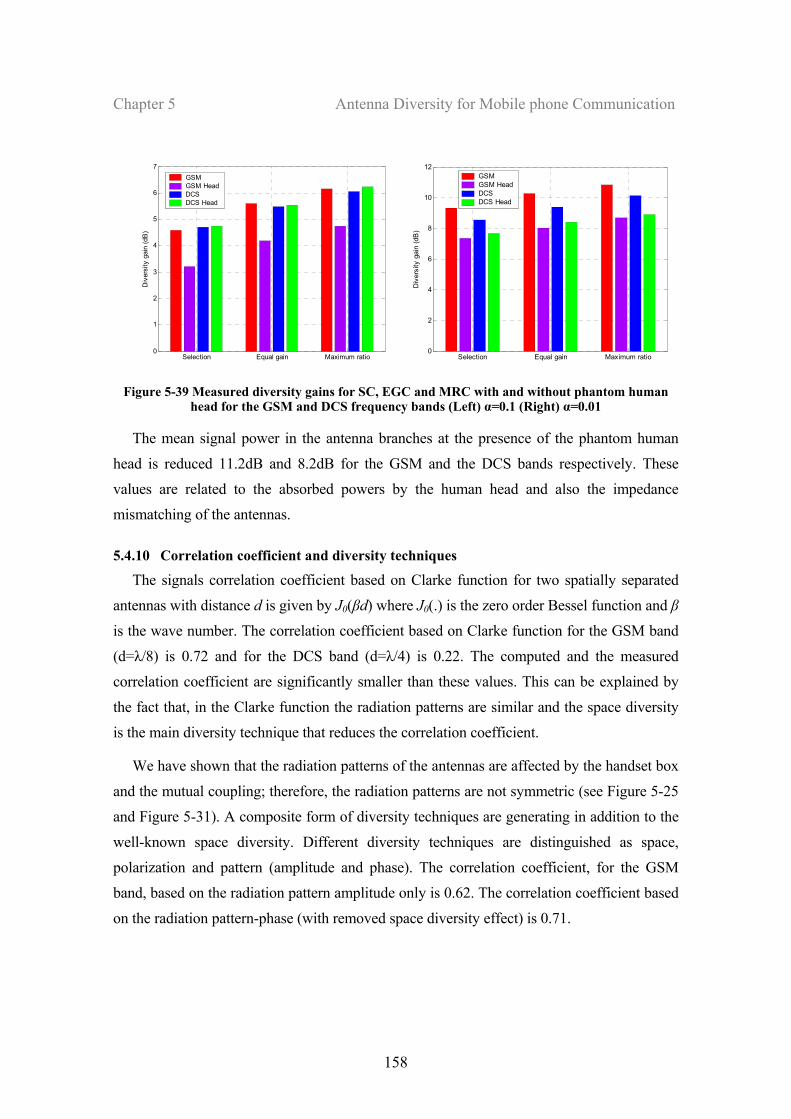
Chapter 5 Antenna Diversity for Mobile phone Communication
158
Selection Equal gain Maximum ratio0
1
2
3
4
5
6
7
Div
ersi
ty g
ain
(dB
)
GSMGSM HeadDCSDCS Head
Selection Equal gain Maximum ratio0
2
4
6
8
10
12
Div
ersi
ty g
ain
(dB
)
GSMGSM HeadDCSDCS Head
Figure 5-39 Measured diversity gains for SC, EGC and MRC with and without phantom human
head for the GSM and DCS frequency bands (Left) α=0.1 (Right) α=0.01
The mean signal power in the antenna branches at the presence of the phantom human
head is reduced 11.2dB and 8.2dB for the GSM and the DCS bands respectively. These
values are related to the absorbed powers by the human head and also the impedance
mismatching of the antennas.
5.4.10 Correlation coefficient and diversity techniques
The signals correlation coefficient based on Clarke function for two spatially separated
antennas with distance d is given by J0(βd) where J0(.) is the zero order Bessel function and β
is the wave number. The correlation coefficient based on Clarke function for the GSM band
(d=λ/8) is 0.72 and for the DCS band (d=λ/4) is 0.22. The computed and the measured
correlation coefficient are significantly smaller than these values. This can be explained by
the fact that, in the Clarke function the radiation patterns are similar and the space diversity
is the main diversity technique that reduces the correlation coefficient.
We have shown that the radiation patterns of the antennas are affected by the handset box
and the mutual coupling; therefore, the radiation patterns are not symmetric (see Figure 5-25
and Figure 5-31). A composite form of diversity techniques are generating in addition to the
well-known space diversity. Different diversity techniques are distinguished as space,
polarization and pattern (amplitude and phase). The correlation coefficient, for the GSM
band, based on the radiation pattern amplitude only is 0.62. The correlation coefficient based
on the radiation pattern-phase (with removed space diversity effect) is 0.71.
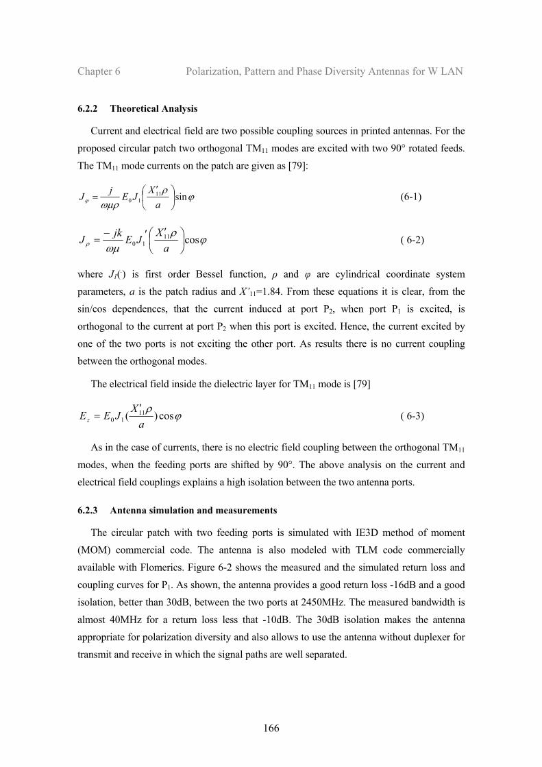
Chapter 6 Polarization, Pattern and Phase Diversity Antennas for W LAN
166
6.2.2 Theoretical Analysis
Current and electrical field are two possible coupling sources in printed antennas. For the
proposed circular patch two orthogonal TM11 modes are excited with two 90° rotated feeds.
The TM11 mode currents on the patch are given as [79]:
ϕρ
ωµρϕ sin1110 ⎟
⎠
⎞⎜⎝
⎛ ′=
aX
JEjJ (6-1)
ϕρ
ωµρ cos1110 ⎟
⎠⎞
⎜⎝⎛ ′′−
=a
XJEjkJ ( 6-2)
where J1(.) is first order Bessel function, ρ and φ are cylindrical coordinate system
parameters, a is the patch radius and X’11=1.84. From these equations it is clear, from the
sin/cos dependences, that the current induced at port P2, when port P1 is excited, is
orthogonal to the current at port P2 when this port is excited. Hence, the current excited by
one of the two ports is not exciting the other port. As results there is no current coupling
between the orthogonal modes.
The electrical field inside the dielectric layer for TM11 mode is [79]
ϕρ
cos)( 1110 a
XJEEz
′= ( 6-3)
As in the case of currents, there is no electric field coupling between the orthogonal TM11
modes, when the feeding ports are shifted by 90°. The above analysis on the current and
electrical field couplings explains a high isolation between the two antenna ports.
6.2.3 Antenna simulation and measurements
The circular patch with two feeding ports is simulated with IE3D method of moment
(MOM) commercial code. The antenna is also modeled with TLM code commercially
available with Flomerics. Figure 6-2 shows the measured and the simulated return loss and
coupling curves for P1. As shown, the antenna provides a good return loss -16dB and a good
isolation, better than 30dB, between the two ports at 2450MHz. The measured bandwidth is
almost 40MHz for a return loss less that -10dB. The 30dB isolation makes the antenna
appropriate for polarization diversity and also allows to use the antenna without duplexer for
transmit and receive in which the signal paths are well separated.
Chapter 6 Polarization, Pattern and Phase Diversity Antennas for W LAN
182
through the measurements. Our study reveals that the pattern diversity based upon the
monopole active element is not a good choice for WLANs that needs larger bandwidth and
also good impedance matching.
0.5 1 1.5 2 2.5 3 3.5 4-12
-10
-8
-6
-4
-2
0
Frequency(GHz)
Ret
urn
Loss
(dB
)
Single DipoleDipole with parasitic elements
(a) (b)
Figure 6-20 (a) The modeled pattern diversity antenna on a finite ground plane with 16-parasitic elements. (b) Return loss versus frequency for single monopole on the ground plane and after
installing the parasitic elements
Considering the above approach we have replaced the simple monopole antenna by a
meander shaped prototype. The meander line technology offers larger bandwidth and also
smaller antenna size. The antenna design is optimized for WLAN applications (at
2450MHz) by good impedance matching at the antenna port and sufficient impedance
bandwidth. Two uncorrelated patterns are generated by selecting an appropriate
configuration of the parasitic rods and connecting or disconnecting the rods to the ground
plane. The AoA for indoor scattering channels is about isotropically distributed; therefore to
have good signal reception all spatial angles should be covered by the antenna patterns.
6.3.2 Main radiator antenna design
Figure 6-21 shows different meanderline and dual-meanderline shaped monopole antennas
on a circular ground plane. The configuration (a) is a single meandered wire antenna (b) is a
dual meander shaped and (c) is a dual meander shape with an open ended configuration.
The horizontal and the vertical lengths of the meander antennas are equally selected. Six
Short circuited elements
Open circuited elements
Space gap
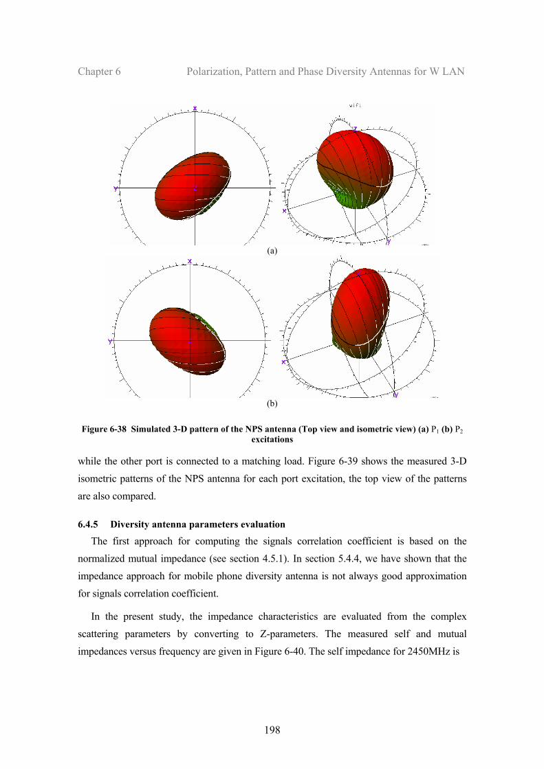
Chapter 6 Polarization, Pattern and Phase Diversity Antennas for W LAN
198
(a)
(b)
Figure 6-38 Simulated 3-D pattern of the NPS antenna (Top view and isometric view) (a) P1 (b) P2 excitations
while the other port is connected to a matching load. Figure 6-39 shows the measured 3-D
isometric patterns of the NPS antenna for each port excitation, the top view of the patterns
are also compared.
6.4.5 Diversity antenna parameters evaluation
The first approach for computing the signals correlation coefficient is based on the
normalized mutual impedance (see section 4.5.1). In section 5.4.4, we have shown that the
impedance approach for mobile phone diversity antenna is not always good approximation
for signals correlation coefficient.
In the present study, the impedance characteristics are evaluated from the complex
scattering parameters by converting to Z-parameters. The measured self and mutual
impedances versus frequency are given in Figure 6-40. The self impedance for 2450MHz is

Chapter 6 Polarization, Pattern and Phase Diversity Antennas for W LAN
214
illustrate too small signals correlation coefficient and consequently good diversity gain. The
measured MEG of the antennas is 1.5dB better than a standard half-wave dipole antenna.
The antennas are appropriate for installing on the access point of the WiFi systems.