Dr. – Ing. Artur Seibt Lagergasse 2/6

A 1030 Vienna Austria email: dr.seibt@aon.at

Fachartikel, erscheint in "Bodo's Power Okt. 14". "DC and AC Signals/Parameters and their correct Representation by Measuring Instruments." 22.6.14 "Do you trust all displays and numbers your measuring instruments show? If the functional principles and/or the calibration of the 6 types of instruments are unknown, gross errors may go undetected. This article points out some common pitfalls." 1. Definitions of AC parameters. Most of today's signals, power voltages and currents are AC and non-sinusoidal as well. It is vital to differentiate between their parameters: 1.1 Average or mean value: this is the arithmetic mean of the signal as measured over a

period or multiples thereof, it is identical to its DC content which is zero for pure AC signals.

1.2 Root-mean-square value: this is the value of a voltage or current which is equivalent to a DC voltage or current when applied to a resistor, i.e. it causes the same amount of power dissipated: Irms = √(1/T ∫ i2 dt).

1.3 Peak value: this is the value of a signal from zero to its maximum. 1.4 Peak-to-peak value: this is the value of a signal from its negative to its positive maxima. 1.5 Crest factor: this is the ratio of the peak to the rms values. This is a vital parameter with

all rms measuring instruments which, if disregarded, causes gross errors. 2. 6 Types of measuring instruments. 2.1 Peak-to-peak displaying instruments: oscilloscopes. 2.2 Peak responding instruments (True peak) 2.3 Peak responding instruments, calibrated rms for sines. 2.4 Average responding instruments (True average) 2.5 Average responding instruments, calibrated rms for sines. 2.6 Rms reading instruments: here the user has to watch out whether they measure "AC

only" or "True rms" = "AC + DC". The majority are of the first type; in this case the user has to measure the "AC only" and the DC values separately and calculate the true rms value by using the familiar formula for uncorrelated signals: Itrue rms = √ (IDC

2 + IrmsAC2 ).

The measurement of the DC component may not be as trivial as it may seem: if a small DC component is buried in a large AC signal a DC instrument may show substantial errors.

2

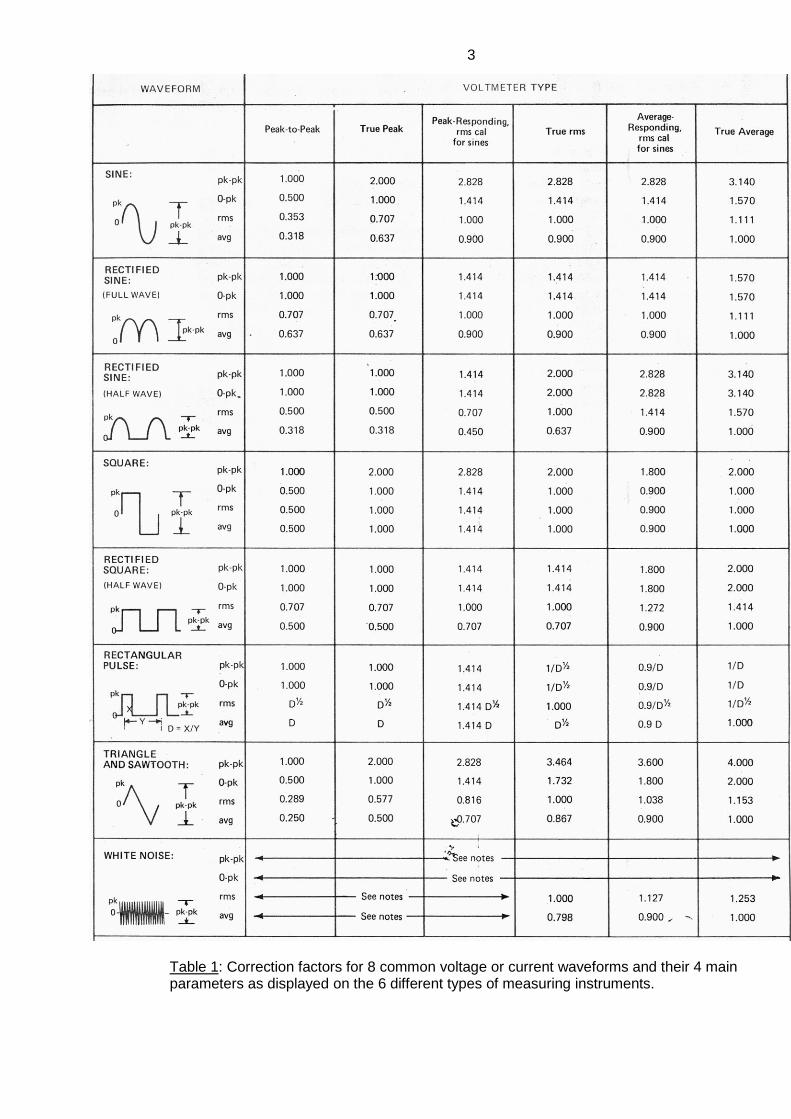
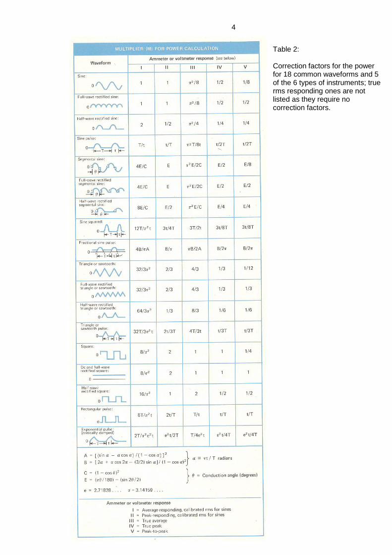
3. Pitfall: Correction factors for non-sinusoidal waveforms required. The most important parameter of a waveform is usually the rms value. While true rms instruments will deliver correct numbers for all waveforms within their specs, this can not be expected from all other types. Most of the average and peak responding types are calibrated rms for (pure) sines, they will indicate false numbers for non-sinusoidal waveforms! In practice, any of the 6 types can be used for non-sinuoidal waveforms if one knows the functional principle and its calibration and applies the proper correction factor. It is highly risky to grab an unfamiliar measuring instrument, because rarely does the front panel inform about how it measures and is calibrated! "Calibrated rms" is rather an indication that it is no true rms instrument, this would be described as "True rms". Table 1 lists the correction factors for the 4 main parameters of 8 common voltage or current waveforms as displayed by the 6 different measuring instruments, Table 2 contains the correction factors for the power. How to use Table 1: Assumed the ac voltmeter available is of the average-responding type, calibrated rms for sines, and the rms value of a sawtooth is desired. The table shows the proper conversion factor 1.038 by which the reading has to be multiplied. But if the sawtooth was first measured on a scope and attributed the value 1.000, a true average-responding instrument would show only 0.25, so the correction factor is 4.000; in other words the reading was a whopping 400 % false. The values for white noise are only approximate because they are measured with a scope. How to use Table 2: If voltage and current are both measured with any of the 5 types of instruments listed (with true rms instruments the factor is always 1), the power will be given by the product of the voltage and current readings times the dimensionless correction factor in the table. If, e.g., a sawtooth voltage across a resistor is measured with an average-responding instrument, calibrated rms for sines, then the power in the resistor is given by: P = V2 /R x 32/3π2 ..( x 1.081.) In case the voltage and the current are measured by differently responding instruments, the power will be given by: P = V x I x √ (FV x FI ) where FV is the factor for the voltmeter and FI is the factor for the ammeter. Both tables demonstrate convincingly, if not shockingly, that a measuring instrument can only be trusted if the user knows how it functions, how it is calibrated, also which limitations must be observed for correct results.

3

Table 1: Correction factors for 8 common voltage or current waveforms and their 4 main parameters as displayed on the 6 different types of measuring instruments.

4

Table 2: Correction factors for the power for 18 common waveforms and 5 of the 6 types of instruments; true rms responding ones are not listed as they require no correction factors.

5

4. Specifications, Resolution, Accuracy. Since the advent of the first instruments with a digital display some decades ago, i.e. digital voltmeters and counters, many manufacturers can not resist the temptation to pretend a higher accuracy by a high number of digits. Customers indeed tend to prefer the higher digit instrument inferring it is the more accurate. A 0.01 % instrument needs only 4 digits, more contain no information. A professional instrument should not display more digits than is justified by its specs. It is the accuracy which determines cost and price because it requires expensive hardware which can not be substituted by software. Calling an instrument e.g. a "0.1 % instrument" is already misleading, because every instrument is specified by an error budget, valid at one specific temperature or within a narrow range and after a specified warming up period.This consists basically of "error of reading" plus "error of full scale" contributions, a temperature coefficient (TC), a time elapsed since the last calibration factor and, with AC instruments, a frequency dependent error. Pitfall: except for true rms instruments, the AC accuracy is only guaranteed for a pure sine wave, extremely rare in practice. As a rule, most errors also depend on the range used. If all error contributions are summed up, the accuracy to be reliably expected may be an order of magnitude lower than advertised! Specsmanship was invented by the measurement instrument and semiconductor industries. Pitfall: Rms instruments display correct results only, if their crest factor = peak/rms spec is not exceeded. A typical measurement is the rms value of a pulse train, e.g. in a SMPS. A crest factor of 4 means that the instrument has a dynamic range 4 times as large as the full scale (fs) value of the range selected. In practice, this means that the rms value may be close to the fs value of a range, but that it is only correct as long as the peaks stay below 4 times the fs value. If the peaks are higher, they will be cut off, and the rms value will be inaccurate. This implies that the available crest factor increases towards the low end of a range. A quick test: downrange the instrument, if the value changes, the first measurement was false. Some instruments show the crest factor. 5. Analog/digital Instruments, Digitizing. The family of analog/digital instruments is large, only a few selected topics can be covered. Analog/digital instruments digitize voltages or currents and show the results on multi-digit displays. They can be categorized into 3 classes: 1. Integrating converters which measure the average of a signal, i.e. the DC component. 2. Instantaneous converters, the object is only the measurement of parameters, then

undersampling is possible, e.g. digital voltmeters or power analyzers. 3. Instantaneous converters, the object is the reconstruction of the signal, this applies to

DSOs. In order to measure the peak, peak-to-peak, rms and derived parameters, in most instruments all inputs are digitized and the calculations performed in the digital domain, it is less expensive, and the data can be used for further processing. For AC fast instantaneous converters are required which are considerably more complicated than the averaging ones and suffer from a variety of errors depicted in Fig. 1.

6

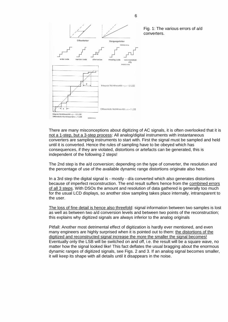
Fig. 1: The various errors of a/d converters.

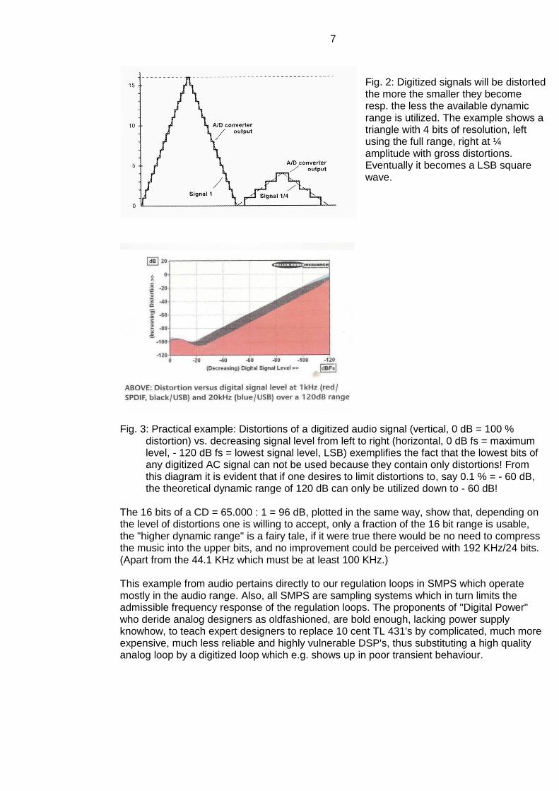
There are many misconceptions about digitizing of AC signals, it is often overlooked that it is not a 1-step, but a 3-step process: All analog/digital instruments with instantaneous converters are sampling instruments to start with. First the signal must be sampled and held until it is converted. Hence the rules of sampling have to be obeyed which has consequences, if they are violated, distortions or artefacts can be generated, this is independent of the following 2 steps! The 2nd step is the a/d conversion; depending on the type of converter, the resolution and the percentage of use of the available dynamic range distortions originate also here. In a 3rd step the digital signal is - mostly - d/a converted which also generates distortions because of imperfect reconstruction. The end result suffers hence from the combined errors of all 3 steps. With DSOs the amount and resolution of data gathered is generally too much for the usual LCD displays, so another slow sampling takes place internally, intransparent to the user. The loss of fine detail is hence also threefold: signal information between two samples is lost as well as between two a/d conversion levels and between two points of the reconstruction; this explains why digitized signals are always inferior to the analog originals Pitfall: Another most detrimental effect of digitization is hardly ever mentioned, and even many engineers are highly surprised when it is pointed out to them: the distortions of the digitized and reconstructed signal increase the more the smaller the signal becomes! Eventually only the LSB will be switched on and off, i.e. the result will be a square wave, no matter how the signal looked like! This fact deflates the usual bragging about the enormous dynamic ranges of digitized signals, see Figs. 2 and 3. If an analog signal becomes smaller, it will keep its shape with all details until it disappears in the noise.

7

Fig. 2: Digitized signals will be distorted the more the smaller they become resp. the less the available dynamic range is utilized. The example shows a triangle with 4 bits of resolution, left using the full range, right at ¼ amplitude with gross distortions. Eventually it becomes a LSB square wave.

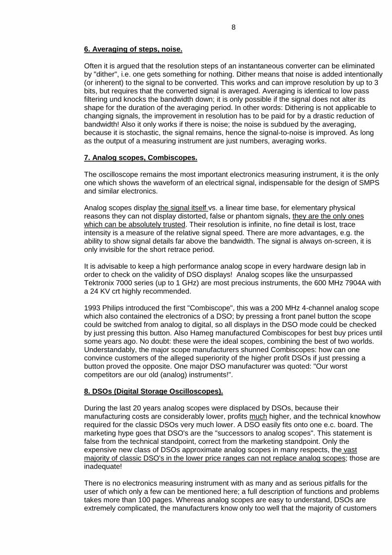
Fig. 3: Practical example: Distortions of a digitized audio signal (vertical, 0 dB = 100 %

distortion) vs. decreasing signal level from left to right (horizontal, 0 dB fs = maximum level, - 120 dB fs = lowest signal level, LSB) exemplifies the fact that the lowest bits of any digitized AC signal can not be used because they contain only distortions! From this diagram it is evident that if one desires to limit distortions to, say 0.1 % = - 60 dB, the theoretical dynamic range of 120 dB can only be utilized down to - 60 dB!

The 16 bits of a CD = 65.000 : 1 = 96 dB, plotted in the same way, show that, depending on the level of distortions one is willing to accept, only a fraction of the 16 bit range is usable, the "higher dynamic range" is a fairy tale, if it were true there would be no need to compress the music into the upper bits, and no improvement could be perceived with 192 KHz/24 bits. (Apart from the 44.1 KHz which must be at least 100 KHz.) This example from audio pertains directly to our regulation loops in SMPS which operate mostly in the audio range. Also, all SMPS are sampling systems which in turn limits the admissible frequency response of the regulation loops. The proponents of "Digital Power" who deride analog designers as oldfashioned, are bold enough, lacking power supply knowhow, to teach expert designers to replace 10 cent TL 431's by complicated, much more expensive, much less reliable and highly vulnerable DSP's, thus substituting a high quality analog loop by a digitized loop which e.g. shows up in poor transient behaviour.

8

6. Averaging of steps, noise. Often it is argued that the resolution steps of an instantaneous converter can be eliminated by "dither", i.e. one gets something for nothing. Dither means that noise is added intentionally (or inherent) to the signal to be converted. This works and can improve resolution by up to 3 bits, but requires that the converted signal is averaged. Averaging is identical to low pass filtering und knocks the bandwidth down; it is only possible if the signal does not alter its shape for the duration of the averaging period. In other words: Dithering is not applicable to changing signals, the improvement in resolution has to be paid for by a drastic reduction of bandwidth! Also it only works if there is noise; the noise is subdued by the averaging, because it is stochastic, the signal remains, hence the signal-to-noise is improved. As long as the output of a measuring instrument are just numbers, averaging works. 7. Analog scopes, Combiscopes. The oscilloscope remains the most important electronics measuring instrument, it is the only one which shows the waveform of an electrical signal, indispensable for the design of SMPS and similar electronics. Analog scopes display the signal itself vs. a linear time base, for elementary physical reasons they can not display distorted, false or phantom signals, they are the only ones which can be absolutely trusted. Their resolution is infinite, no fine detail is lost, trace intensity is a measure of the relative signal speed. There are more advantages, e.g. the ability to show signal details far above the bandwidth. The signal is always on-screen, it is only invisible for the short retrace period. It is advisable to keep a high performance analog scope in every hardware design lab in order to check on the validity of DSO displays! Analog scopes like the unsurpassed Tektronix 7000 series (up to 1 GHz) are most precious instruments, the 600 MHz 7904A with a 24 KV crt highly recommended. 1993 Philips introduced the first "Combiscope", this was a 200 MHz 4-channel analog scope which also contained the electronics of a DSO; by pressing a front panel button the scope could be switched from analog to digital, so all displays in the DSO mode could be checked by just pressing this button. Also Hameg manufactured Combiscopes for best buy prices until some years ago. No doubt: these were the ideal scopes, combining the best of two worlds. Understandably, the major scope manufacturers shunned Combiscopes: how can one convince customers of the alleged superiority of the higher profit DSOs if just pressing a button proved the opposite. One major DSO manufacturer was quoted: "Our worst competitors are our old (analog) instruments!". 8. DSOs (Digital Storage Oscilloscopes). During the last 20 years analog scopes were displaced by DSOs, because their manufacturing costs are considerably lower, profits much higher, and the technical knowhow required for the classic DSOs very much lower. A DSO easily fits onto one e.c. board. The marketing hype goes that DSO's are the "successors to analog scopes". This statement is false from the technical standpoint, correct from the marketing standpoint. Only the expensive new class of DSOs approximate analog scopes in many respects, the vast majority of classic DSO's in the lower price ranges can not replace analog scopes; those are inadequate! There is no electronics measuring instrument with as many and as serious pitfalls for the user of which only a few can be mentioned here; a full description of functions and problems takes more than 100 pages. Whereas analog scopes are easy to understand, DSOs are extremely complicated, the manufacturers know only too well that the majority of customers

9

lack the specific scope technology knowledge, advertising and manuals withhold salient facts, unfounded performance claims and misleading designations leave the customers in the dark. DSO's can never display a signal in real time like analog scopes, only a more or less distorted reproduction after the signal has disappeared. Users are blinded and attracted by the pc features, but less aware of the shortcomings as a measuring instrument. The only real advantages of DSOs are the ability to store waveforms and to replay them out of memory. Their other features are due to the built-in pc, if the reconstructed waveform is an artefact, the digitized data will also be false as well as all calculations derived; garbage in, garbage out applies. The built-in pc, however, allows, e.g., to calculate parameters like the rms value, power from two inputs, to generate a FFT, to decode buses etc., and this increases the usefulness enormously. Analog scopes are "only" measuring instruments, they lack the pc features. There are two classes of DSOs meanwhile: The sequentially processing "classic" DSOs: Most low- and middle-priced models are classic DSOs which consist in principle of a pc with a multi-channel analog front end, a sampler and a 8 bit a/d converter for each input, a memory and a LCD or monitor display. They acquire a signal by sampling, a/d convert it, store it, reconvert it and display it. This long processing time allows only acquisition rates from some ten to some thousand per second, i.e. less than 1 % of the time, more than 99 % the scope is blind. The parallel processing top models (DPOs and similar ones): Realizing that the basic problems of DSOs can not even be solved, if ever faster processing becomes available, Tektronix was the first to massively invest in parallel processing hardware in order to emulate analog scopes as much as possible. In 1994 the first "Instavu" scope appeared, later called "Real-Time" and then "DPO". In short: this class of scope contains additionally the equivalent of the electronics of an analog scope: the acquisition system runs at the speed of the signal trigger up to a maximum of 400 K which is the same as that of the best analog scopes, the information is rasterized in 3 dimensions, the third is the frequency of occurence, which modulates the trace intensity as in analog scopes. Because of MB's of memory, the sampler running at full speed and the masses of acquisitions compiled in the raster memory, false displays are unlikely. Every 1/30th of a second a copy is transferred to the display. These scopes react as fast as analog scopes and emulate the phosphor properties, hence the name, they also catch rare events as fast. They are superior in that respect because the digital memory stores the event. "Real-Time" refers to this sampling mode, a display of the signal in real time is impossible, no matter how much hard- and software is invested; the signal reconstruction appears on the screen after the signal has long since disappeared. Customers are expected to understand that these DSOs show the signal in real time like analog scopes. 8.1 Sampling. As mentioned in chapter 5, the signal must be sampled and held before it can be a/d converted. The process of sampling is similar to mixing and correlation, it is a transformation method. Any information can be visualized as a brick-like volume in a three-axis coordinate system with the axes amplitude, bandwidth and time. While keeping the volume constant, the three parameters can be exchanged. With sampling the amplitude is held constant, the bandwidth is increased at the expense of time, in other words: the high frequencies are mixed down into the low frequency range (GHz to some hundred to some thousand Hz).

10

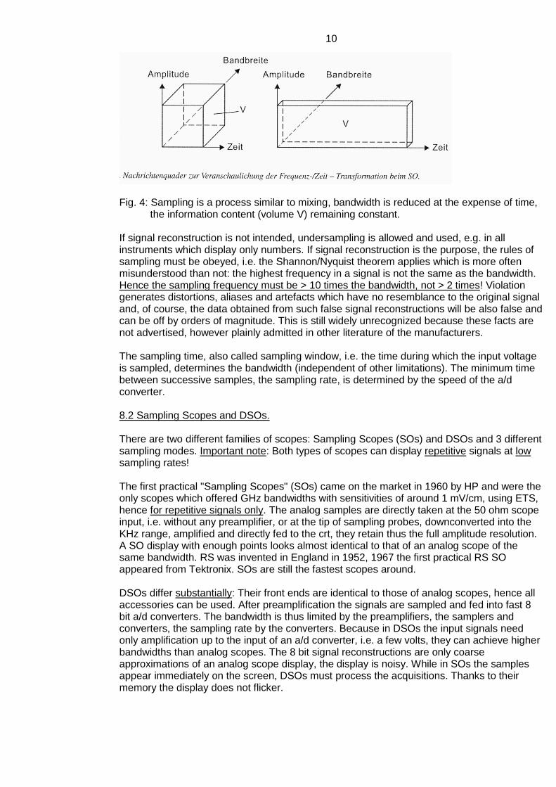
Fig. 4: Sampling is a process similar to mixing, bandwidth is reduced at the expense of time,

the information content (volume V) remaining constant. If signal reconstruction is not intended, undersampling is allowed and used, e.g. in all instruments which display only numbers. If signal reconstruction is the purpose, the rules of sampling must be obeyed, i.e. the Shannon/Nyquist theorem applies which is more often misunderstood than not: the highest frequency in a signal is not the same as the bandwidth. Hence the sampling frequency must be > 10 times the bandwidth, not > 2 times! Violation generates distortions, aliases and artefacts which have no resemblance to the original signal and, of course, the data obtained from such false signal reconstructions will be also false and can be off by orders of magnitude. This is still widely unrecognized because these facts are not advertised, however plainly admitted in other literature of the manufacturers. The sampling time, also called sampling window, i.e. the time during which the input voltage is sampled, determines the bandwidth (independent of other limitations). The minimum time between successive samples, the sampling rate, is determined by the speed of the a/d converter. 8.2 Sampling Scopes and DSOs. There are two different families of scopes: Sampling Scopes (SOs) and DSOs and 3 different sampling modes. Important note: Both types of scopes can display repetitive signals at low sampling rates! The first practical "Sampling Scopes" (SOs) came on the market in 1960 by HP and were the only scopes which offered GHz bandwidths with sensitivities of around 1 mV/cm, using ETS, hence for repetitive signals only. The analog samples are directly taken at the 50 ohm scope input, i.e. without any preamplifier, or at the tip of sampling probes, downconverted into the KHz range, amplified and directly fed to the crt, they retain thus the full amplitude resolution. A SO display with enough points looks almost identical to that of an analog scope of the same bandwidth. RS was invented in England in 1952, 1967 the first practical RS SO appeared from Tektronix. SOs are still the fastest scopes around. DSOs differ substantially: Their front ends are identical to those of analog scopes, hence all accessories can be used. After preamplification the signals are sampled and fed into fast 8 bit a/d converters. The bandwidth is thus limited by the preamplifiers, the samplers and converters, the sampling rate by the converters. Because in DSOs the input signals need only amplification up to the input of an a/d converter, i.e. a few volts, they can achieve higher bandwidths than analog scopes. The 8 bit signal reconstructions are only coarse approximations of an analog scope display, the display is noisy. While in SOs the samples appear immediately on the screen, DSOs must process the acquisitions. Thanks to their memory the display does not flicker.

11

8.3 Sampling modes: Equivalent Time Sampling (ETS): This is an ingenious stroboscopic method, invented 1880 in France; the signal must be repetitive, not necessarily periodic, and must not change its shape. The scope takes one sample along the waveform at each repitition, stepping in time along the waveform, so that it may take hundreds to millions of repititions and some time until the whole waveform has been acquired and displayed once by the scope. This method does not require a fast sampling rate, in fact the sampling rate is independent of the bandwidth, it may be chosen such that the waveform can be slowly drawn on a plotter, even manual scanning is possible. These early instruments typically ran at max. appr. 100 KHz. In this mode SOs and DSOs achieve the highest bandwidths, and those are advertised without explaining that the signals must be repetitive with the same shape. Quite often, fictitious high sampling rates are quoted for ETS. ETS being a stroboscopic method, the time base can extend to infinity. In SOs a pretrigger or a delay line is required in order to show the triggering slope of the signal. Aliases and fancy pictures can be easily produced. All signals which change from period to period can not be reproduced correctly, e.g. modulated signals, in SMPS e.g. signals which are modulated by the line frequency, an oscillating regulation loop etc. Output ripple which typically consists of switching frequency, line frequency and hf components up to e.g. 300 MHz is impossible to measure in this mode. Realizing that, in practice, most signals are repetitive, one can get quite far with ETS. Pitfall: Especially in case of low-cost DSOs the bandwidth advertised is only valid in ETS/RS modes! Random Sampling (RS): The difference to ETS: samples are not taken sequentially along the waveform but randomly. This yields two advantages: it is possible to display the triggering slope of the waveform without a delay line, a precondition for bandwidths beyond around 1 GHz, secondly the probability of stable displays of aliases and other phantoms is low. Real Time Sampling (RTS): This is the "real" sampling method for which the Shannon/Nyquist theorem is valid and which is needed for single shot captures. This has nothing to do with real time signal display of which all DSOs are incapable! Assumed a 500 MHz signal, e.g. a sine, shall be captured once in the RTS mode: if the sampling rate would be a mere 1 GS/s, there would be just 2 points on the screen! The user is invited to draw any waveform through these 2 points, in other words: the display is absolutely worthless. The true meaning of the Nyquist theorem is that it implies knowledge about the waveform: it is a sine, and this the reason why it says that the highest harmonic in the signal must stay below half the sampling rate, the highest harmonic is a sine. It is now apparent that a much higher sampling rate than Nyquist is necessary if one desires a usable signal reconstruction. Normally, a low pass filter must precede the sampler, this is impractical at high frequencies and for another reason: any scope must have a true Gaussian frequency response, which falls off very gradually, any attempt at a steeper roll-off causes pulse distortions. For this reason it is accepted meanwhile that the sampling frequency should be at least 10 times the bandwidth, at this point the response is so far down that aliasing is hardly likely. (In some modern DSOs the frequency response is "polished up" by software! Others have a "maximally flat" response in order to quote a higher bandwidth, accepting the pulse distortions.) A 5 GS/s scope can acquire 10 points of a 500 MHz signal, e.g. a sine, at a sweep speed of 0.2 ns/cm which spreads the 2 ns period over the screen. Because the DSOs mostly use linear interpolation, the 10 points are connected by straight lines, the result does not look like a sine, it is severely distorted. Without the interpolation, there would be just 1 point per cm, this would alert the user that this is all the information the instrument could gather. A 50 MHz signal would produce 100 points and a relatively good replica. Depending on the waveform the number of points varies which are necessary for a usable display. Obviously, 10 times the bandwidth is not enough! Manufacturers have always claimed they could reconstruct

12

waveforms by ingenious interpolation algorithms even with 2.5 points; such methods work only for certain waveshapes, i.e. the user is expected to already know the waveform and select a fitting interpolation. If he knows the waveform, he does not need the scope. While the single shot results are only useful for > 25 points, the instruments use ETS resp. RS for repetitive waveforms to fill the screen with enough points. With DPO-class DSOs the sampler runs at its full speed, so ten signal repititions will yield 100 points. 8.4 Serious pitfall: Advertised and actual sampling rates and bandwidths. All advertising, catalog and manual specs say e.g. "Max. sampling rate 5 GS/s, bandwidth 500 MHz". Most people overlook the "max." preceding the sampling rate and, worse, do not realize that it must also read "max. bandwidth"! This is fatal: In contrast to analog scopes the bandwidth of DSOs is not constant, because the sampling rate is not constant, it can never be greater than about 1/10 the actual sampling rate! Any capture memory is of limited size; if the instrument runs at its maximum sampling rate, the memory will be filled after a finite time; if this time is shorter than the time for a screen width expressed in time, the DSO must decrease its sampling rate. The lower cost DSOs even of renowned manufacturers usually contain only 1 to 10 K of memory, because these are low-cost high-noise analog (!) shift register memories (CCD's = charge-coupled devices) which also contribute signal distortions of their own. Now there is an Iron rule for all DSOs: Actual sampling rate = Memory/sweep speed (e.g. 5 ms/cm) x 10 cm (horiz. axis) Note that the "maximum sampling rate" does not appear in this equation, In SMPS work it is often necessary to use lower sweep rates like 5 ms/cm in order to see line frequency related or motor waveforms. With a mere 2.5 KB of memory (this is the size in a whole range of DSOs of a leading manufacturer!) the maximum sampling rate of e.g. 5 GS/s shrinks down to an actual sampling rate e.g. of 50 KS/s., hence the bandwidth is reduced from the advertised 500 MHz to a mere 5 KHz! What use is a 5 KHz scope? At 20 ms/cm only a sampling rate of 12.5 KHz is left over, the bandwidth is 1.25 KHz! Fig. 6 shows an example of everyday work on offline SMPS with a PFC; this is the current waveform in the PFC choke, consisting of a 100 Hz half sine and the superposed e.g. 125 KHz sawtooth current.

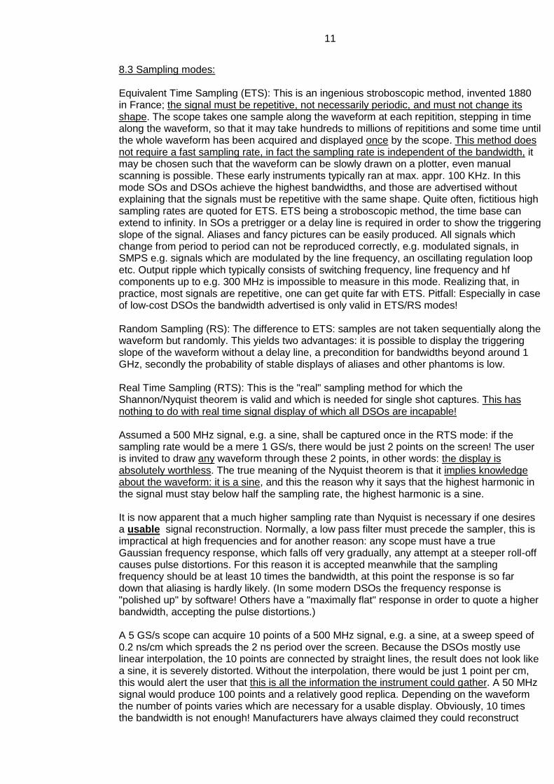
Fig. 6: Choke current of a 50 Hz - PFC at 2 ms/cm.

Any analog scope or a DPO-like type will display the correct waveform. Not so the low cost DSO: with 5 KHz bandwidth left it can only show the 100 Hz half sine, the 125 KHz would be totally lost, resp. only artefacts or phantoms will show up. This is the truth which will probably shock many readers who disposed of their analog scopes, bought the "successors" and thought that with a "500 MHz" DSO they could easily display signals in the hundred KHz range! Of course, this is neither advertised nor mentioned in manuals, but has been admitted ever since in other literature of the leading manufacturers. At such low sampling rates any number of grotesque artefacts can be easily produced. If an engineer working on such circuits has only this inadequate DSO, has no access to a better one or an analog scope, he must stop working - hopefully he realized the false displays. Consequence: If any DSOs with less than appr. 1 MB should be in use in SMPS (or similar electronics) design or test labs, they should be scrapped and replaced! Engineers' time is too

13

precious and costly to waste for chasing DSO phantom displays down. Although competition forced manufacturers recently to increase memory sizes, e.g. a series of 2014 DSOs of a leading manufacturer between 5 and 10,000 E features only 10 KB for all models! Quite often, the vital memory depth is not even specified! All numbers derived from the false reconstructions will also be false. Figs. 5 and 6 and Table 3 show examples.

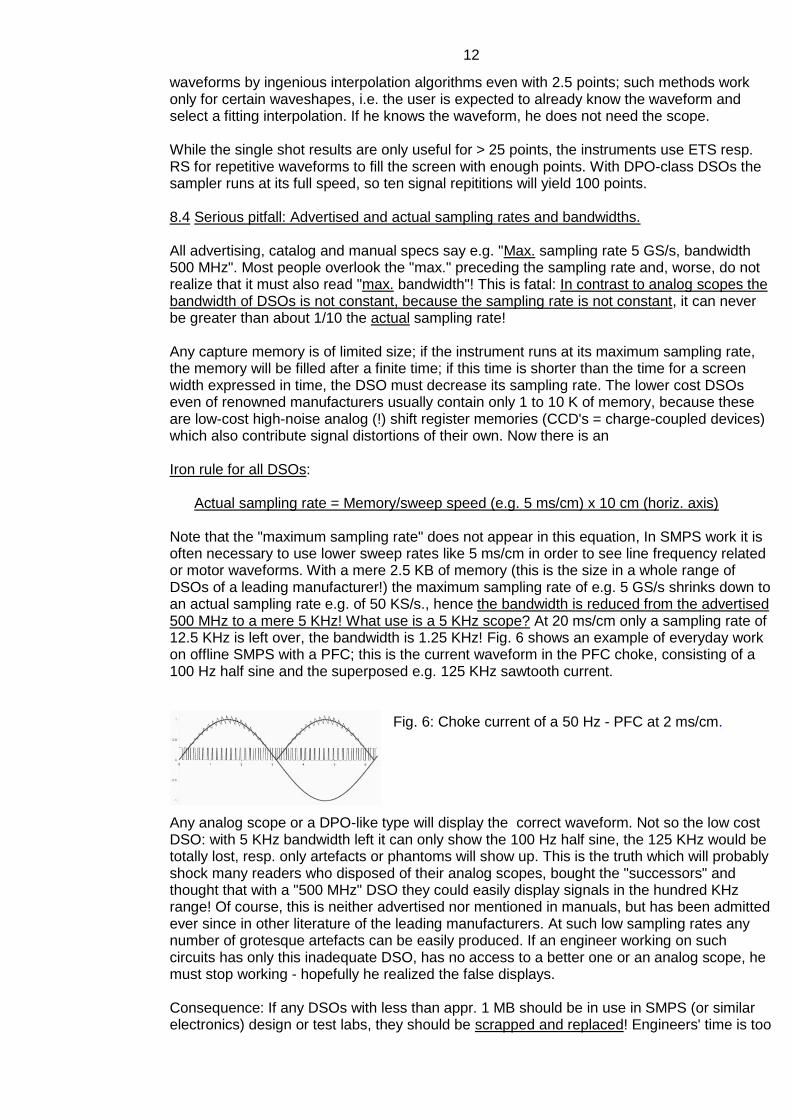
Fig. 5: Alias of a 10 MHz sine, modulated with 1 KHz 80 % at a sweep speed of 100 us/cm, the actual sampling rate is 100 KHz. No resemblance to the true waveform. The DSO is a 2 GS/s 500 MHz type. Display stopped.

Fig. 6: Same signal at 0.5 ms/cm, no stable display possible, because of the AM each period is different from the preceding one. Actual sampling rate 100 KHz. Display running.

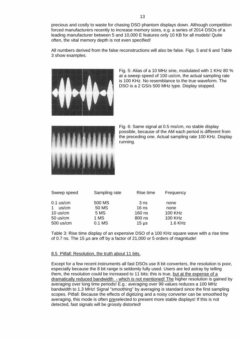
Sweep speed Sampling rate Rise time Frequency 0.1 us/cm 500 MS 3 ns none 1 us/cm 50 MS 16 ns none 10 us/cm 5 MS 160 ns 100 KHz 50 us/cm 1 MS 800 ns 100 KHz 500 us/cm 0.1 MS 15 μs 1.6 KHz Table 3: Rise time display of an expensive DSO of a 100 KHz square wave with a rise time of 0.7 ns. The 15 μs are off by a factor of 21,000 or 5 orders of magnitude! 8.5 Pitfall: Resolution, the truth about 11 bits. Except for a few recent instruments all fast DSOs use 8 bit converters, the resolution is poor, especially because the 8 bit range is seldomly fully used. Users are led astray by telling them, the resolution could be increased to 11 bits; this is true, but at the expense of a dramatically reduced bandwidth - which is not mentioned! The higher resolution is gained by averaging over long time periods! E.g.: averaging over 99 values reduces a 100 MHz bandwidth to 1.3 MHz! Signal "smoothing" by averaging is standard since the first sampling scopes. Pitfall: Because the effects of digitizing and a noisy converter can be smoothed by averaging, this mode is often preselected to present more stable displays! If this is not detected, fast signals will be grossly distorted!

14

Averaging reduces noise. The bulk of the noise is contributed by the a/d converter, so, also here, there is a sharp distinction between low-cost and expensive DSOs: the best converter is the flash or parallel converter, which is the most expensive one, the worst converters are CCD plus slow a/d converter combinations which are by far the cheapest - in both meanings of the word! A CCD (charge-coupled device) is an analog MOS shift register, i.e. a cheap ic. The input signal is fed into the CCD at the sampling speed, after the acquisition the CCD is slowly read out into an a/d converter, thus circumventing costly fast converters. Like all MOS CCDs are very noisy, also the charge packets which are shifted through the register interact, this causes signal distortions which depend on the signal shape. Most low-cost DSOs, also from renowned manufacturers, use CCDs which is the main reason that their memories are limited to 1 to 10 K; he who may think that such small memories are not offered any more is invited to look into the 2014 catalogs, also of major distributors.. 9. Some hints about what to watch out for when using DSOs. 1. Before you use a DSO, study the specs, look up the memory size, use the "Iron Rule"

formula to find out from which sweep speed downward the sampling rate will be reduced. If the size is < 1 MB, take or buy another one! If you can not find the memory size spec, do not use the scope. The actual sampling rate must be >= 10 times the bandwidth at all sweep speeds you use. The frequency content in a switching transistor's drain voltage or current may well extend to > 100 MHz, the same is true for the ripple. Do not settle for less than 100 MHz/1 GS/s at your slowest sweep speed..

Example: A well known German semiconductor firm issued a data sheet for a SMPS ic, it

claimed that the firm had invented a new gate drive circuit for switching mosfets which eliminated the start current spike in flyback circuits. For proof there was a screen shot from a DSO of a leading DSO firm which indeed showed the switch current without that spike. But the actual sampling rate of 25 MS/s was displayed on-screen! Hence the bandwidth was a mere 2.5 MHz resp. the rise time 140 ns. No wonder that the spike which is only a few ten ns wide remained invisible! So this DSO ("successor to analog scopes") made the engineer believe he had invented something, probably his firm applied for a patent. Of course, measured with an analog scope, there was the spike, high as a tower!

2. If you suspect a false display or false numbers, change the sweep speed both ways, false

displays will show up 3. If a picture shows steps in signal slopes, this is a clear sign of an insufficient sampling

rate, this display is false! There was only one DSO firm which showed the actual sampling rate on the screen, meanwhile not any more. It is mostly difficult for the user to find the actual sampling rate in the menus.

4. If the picture shows straight lines with sharp edges, there are too few points for a useful

reconstruction, the display is false. Search for the "points display" in the menu, i.e. switch off the interpolation, then it will become apparent how many points there are.

5. If the picture is noisy, it's probably the DSO; do not trust a noisefree trace without a signal,

the software probably sets the display to zero. There is no other way to find out where the noise comes from but to check with an analog scope. Using the averaging modes of the DSO decreases the bandwidth as explained and may distort the signal.

6. If you are working with fast signals, make sure that all averaging functions are switched

off, they may be preselected, otherwise the signals will be distorted.

15

8. DSO traces are evenly bright, they contain no signal information, hence fast signal slopes will also be evenly bright. (DPO-class DSOs emulate the intensity modulation of analog scopes.)

Fig. 1: Hier bitte statt Offsetfehler "offset error", statt Steigungsfehler "slope error", statt Integrale Nichtlinearität "Integral nonlinearity", statt Differentielle Nichtlinearität "Differential nonlinearity" einsetzen, alles andere bleibt. Bitte Bezeichnungen ersetzen: Statt Bandbreite bandwidth, statt Zeit time. Die Zeile unter dem Bild löschen.

16

Lagergasse 2/6 A-1030 WIEN (VIENNA) AUSTRIA

TEL.: +43 1 505 8186 FAX.: +43 1 503 7084 GSM A: +43 699 11835174 GSM D: +49 172 810 2117

e-mail: dr. seibt@aon.at