Embed Size (px)
Citation preview
Dynamic Modeling and Control of VSC-basedMulti-terminal DC Networks
Sılvio Miguel Fragoso Rodrigues
Dissertacao para a obtencao de Grau de Mestre em
Engenharia Electrotecnica e de Computadores
Juri
Presidente: Prof. Doutor Paulo Jose da Costa BrancoCoorientador: Prof. Doutor Rui Manuel Gameiro de CastroVogal: Prof. Doutora Sonia Maria Nunes dos Santos Paulo Ferreira Pinto
December 2011

This document was prepared using LATEX.
Dynamic Modeling and Control of VSC-basedMulti-terminal DC Networks
Sılvio Miguel Fragoso Rodrigues
Dissertacao para a obtencao de Grau de Mestre em
Engenharia Electrotecnica e de Computadores
Dissertacao realizada sob a orientacao de:
Orientador: Prof.dr.ir. P. BauerCoorientador: Eng. Rodrigo Teixeira PintoCoorientador: Prof. Doutor Rui Manuel Gameiro de Castro
December 2011

This document was prepared using LATEX.

Acknowledgments
First of all I want to express my gratefulness to Eng. Rodrigo Teixeira Pinto and to Prof. Paul Bauer
for the opportunity of finishing my study at TUDelft. I am grateful for the vote of trust, and for all the
support and comprehension through the development of this thesis.
A word to my Portuguese coordinator Prof. Rui Castro who has been a very kind and supportive person
since the beginning. He also trusted me and my capabilities while the development of this dissertation.
An enormous and generous thank to all my friends that have been by my side all this years. A special
thanks to Henrique Silva, Ricardo Grizonic, Pedro Carreira, Joao Falcao, Ricardo Batista, Joana Botelho,
Paulo Chainho, Duarte Martins, Andre Grilo and Joao Bastos. There are a lot more and despite the fact
that their names are not here they were not forgotten.
I would also like to mention all the friendships that I have done during my staying in the Netherlands,
special my friends from JvB27 and my house-mates at JvB89. They always made me feel at home and
were, and will continue to be, very good friends of mine.
Last but not least I would like to thank my parents. They have supported me during my entire life and
worked hard to keep me in school. To them a special thank you.
i
Resumo
Com o aumento da procura por energia electrica por todo o mundo devido nao so a cada vez maior
dependencia energetica dos paıses industrializados como tambem devido ao grande desenvolvimento de
paıses como a India e a China, a producao de energia electrica tem indubitavelmente que acompanhar essa
subida [1]. Neste momento, fontes de energia renovavel sao uma forte aposta na Europa [2]. Uma destas
fontes e a energia eolica cuja tecnologia, bastante amadurecida, ja consegue rivalizar a nıvel economico
com as fontes de energia de origem nao renovavel [3]. Por outro lado a energia eolica offshore apenas
agora comeca a dar os seus primeiros passos como tecnologia de escolha para o transporte em corrente
contınua de energia proveniente dos parques eolicos mais distantes da costa. No entanto, em 2020, e
esperado que os parques eolicos offshore produzam um terco de toda a energia eolica [4].
Actualmente existem mais de 100 sistemas de transmissao em corrente contınua mas no entanto apenas 3
deles tem 3 terminais sendo os restantes sistemas ponto a ponto [5]. Com os recentes avancos na tecnologia
CFT (conversores de fonte de tensao), redes multi-terminal em corrente contınua poderao ser criadas com
maior facilidade. O espaco ocupado por estes equipamentos e mais reduzido quando comparado com o
espaco utilizado pelos CFC (conversores de fonte de corrente) o que traz grandes vantagens a nıvel offshore
pois os custos de instalacao e manutencao sao bastante elevados [6][7].
Nos proximos anos serao instalados dezenas de parques eolicos offshore por toda a Europa [4]. Devido
as vantagens que a tecnologia CFT apresenta face as restantes opcoes, existe uma forte possibilidade que
seja essa a tecnologia escolhida para estar presente nos parques [8]. Tal situacao serve de mote para que
sejam estudados os metodos de simulacao e controlo deste tipo de sistemas. Como tal, esta tese tem
como objetivo o estudo de modelos que sejam capazes de simular com detalhe necessario os sistemas
electricos de parques eolicos offshore, os conversores e a rede multi-terminal. Os metodos de controlo
de todo o sistema tambem serao estudados e serao apresentadas varias tecnicas para controlar a tensao
dentro da rede. Deste modo sera possıvel aos varios paıses ligados a rede multi-terminal nao so receber
energia, proveniente dos parques eolicos offshore segundo um certo criterio de partilha, como tambem
transaccionar energia entre si.
Palavras-Chave: VSC-HVDC, Rede Multi-terminal, Offshore, Modelo Equivalente, Estrategias
de Controlo.
ii
Abstract
With the increased need for electric energy all over the world, not only because of the higher energetic
dependency of the industrialized countries, but also due to the enormous development of countries such
as India and China, the production of electric energy has, without question, to increase as well [1].
Nowadays, renewable energy sources are being installed at a huge rate in Europe [2]. One of these
renewable sources is the onshore wind energy, whose technology, already developed, is able to compete in
an economic way with the non-renewable energy sources [3]. On the other hand, the offshore wind energy
is now giving its first steps as the technology of choice for the power transmission in direct current from
the distant offshore wind farms. However, in 2020, it is expected that one third of all the wind energy
will be transmitted from offshore wind farms [4].
Nowadays, there are more than 100 transmission systems in direct current. However, only 3 of them
have 3 terminals, while all the others are point-to-point systems [5]. With the recent developments in
the VSC technology, MTDC grids may be more easily created. The space required by the equipments of
this technology is smaller when compared to the space used by the CSCs. Therefore, the installation and
maintenance costs are reduced [6][7].
In the next years, dozens of offshore wind farms will be installed all over Europe [4]. Due to the technologic
advantages that VSCs have when compared to the other options, there is a strong possibility that it will
be the technology chosen to connect the offshore wind farms [8]. Such assumption intensifies the need
of studying and simulating the control methods for these systems. Therefore, the purpose of the present
thesis is the study of models that are able to simulate with the necessary detail, the electric systems of
the offshore wind farms, the converters and the DC grid. The control methods of the system will also be
studied and several methods to control the DC voltage will be presented. This way, it will be possible for
the several countries connected to the multiterminal DC grid not only to receive energy from the offshore
wind farms, according a certain criteria, but also to trade energy with each other.
Keywords: VSC-HVDC, Multi-terminal Network, Offshore, Equivalent Model, Control strategies.
iii

Contents
Acknowledgments . . . . . . . . . . . . . . . . . . . . . . . . . . . . . . . . . . . . . . . . . . . . i
Resumo . . . . . . . . . . . . . . . . . . . . . . . . . . . . . . . . . . . . . . . . . . . . . . . . . ii
Abstract . . . . . . . . . . . . . . . . . . . . . . . . . . . . . . . . . . . . . . . . . . . . . . . . . iii
Contents . . . . . . . . . . . . . . . . . . . . . . . . . . . . . . . . . . . . . . . . . . . . . . . . . vi
List of Tables . . . . . . . . . . . . . . . . . . . . . . . . . . . . . . . . . . . . . . . . . . . . . . vii
List of Figures . . . . . . . . . . . . . . . . . . . . . . . . . . . . . . . . . . . . . . . . . . . . . x
List of Acronyms . . . . . . . . . . . . . . . . . . . . . . . . . . . . . . . . . . . . . . . . . . . . xi
List of Symbols . . . . . . . . . . . . . . . . . . . . . . . . . . . . . . . . . . . . . . . . . . . . . xiv
1 Introduction 1
1.1 Motivation . . . . . . . . . . . . . . . . . . . . . . . . . . . . . . . . . . . . . . . . . . . . 1
1.2 Thesis objective and contributions . . . . . . . . . . . . . . . . . . . . . . . . . . . . . . . 2
1.3 Publications . . . . . . . . . . . . . . . . . . . . . . . . . . . . . . . . . . . . . . . . . . . . 2
1.4 Thesis layout . . . . . . . . . . . . . . . . . . . . . . . . . . . . . . . . . . . . . . . . . . . 2
1.5 State of the Art . . . . . . . . . . . . . . . . . . . . . . . . . . . . . . . . . . . . . . . . . . 3
1.6 Current Status of Offshore Wind Energy . . . . . . . . . . . . . . . . . . . . . . . . . . . . 4
1.7 Offshore Transmission technologies . . . . . . . . . . . . . . . . . . . . . . . . . . . . . . . 5
1.7.1 HVAC . . . . . . . . . . . . . . . . . . . . . . . . . . . . . . . . . . . . . . . . . . . 5
1.7.2 LCC-HVDC . . . . . . . . . . . . . . . . . . . . . . . . . . . . . . . . . . . . . . . . 6
1.7.3 VSC-HVDC . . . . . . . . . . . . . . . . . . . . . . . . . . . . . . . . . . . . . . . . 6
1.8 Comparison of transmission systems: HVAC vs HVDC . . . . . . . . . . . . . . . . . . . . 7
1.9 Comparison of DC transmission systems: LCC- vs VSC-HVDC . . . . . . . . . . . . . . . 8
1.10 Transmission cables . . . . . . . . . . . . . . . . . . . . . . . . . . . . . . . . . . . . . . . 9
1.11 Wind Energy in Portugal . . . . . . . . . . . . . . . . . . . . . . . . . . . . . . . . . . . . 11
iv
2 VSC-HVDC Equivalent Model and Controllers 13
2.1 Introduction . . . . . . . . . . . . . . . . . . . . . . . . . . . . . . . . . . . . . . . . . . . . 13
2.2 VSC-HVDC Transmission System . . . . . . . . . . . . . . . . . . . . . . . . . . . . . . . 13
2.2.1 AC Breakers . . . . . . . . . . . . . . . . . . . . . . . . . . . . . . . . . . . . . . . 14
2.2.2 AC Filters . . . . . . . . . . . . . . . . . . . . . . . . . . . . . . . . . . . . . . . . . 14
2.2.3 Transformer . . . . . . . . . . . . . . . . . . . . . . . . . . . . . . . . . . . . . . . . 14
2.2.4 Phase Reactor . . . . . . . . . . . . . . . . . . . . . . . . . . . . . . . . . . . . . . 15
2.2.5 Voltage Source Converter . . . . . . . . . . . . . . . . . . . . . . . . . . . . . . . . 15
2.2.6 DC Capacitor . . . . . . . . . . . . . . . . . . . . . . . . . . . . . . . . . . . . . . . 17
2.2.7 DC Cable . . . . . . . . . . . . . . . . . . . . . . . . . . . . . . . . . . . . . . . . . 17
2.2.8 DC Chopper . . . . . . . . . . . . . . . . . . . . . . . . . . . . . . . . . . . . . . . 18
2.3 Voltage Source Converter’s equivalent model . . . . . . . . . . . . . . . . . . . . . . . . . 18
2.3.1 Equivalent model of the VSC AC side . . . . . . . . . . . . . . . . . . . . . . . . . 18
2.3.2 Equivalent model of the VSC DC side . . . . . . . . . . . . . . . . . . . . . . . . . 22
2.4 The control system of the VSC-HVDC . . . . . . . . . . . . . . . . . . . . . . . . . . . . . 22
2.4.1 Inner Current Controller . . . . . . . . . . . . . . . . . . . . . . . . . . . . . . . . . 23
2.4.2 Outer Controllers . . . . . . . . . . . . . . . . . . . . . . . . . . . . . . . . . . . . . 24
2.4.3 VSC Controllers Bandwidth . . . . . . . . . . . . . . . . . . . . . . . . . . . . . . . 26
2.4.4 Current Limiter . . . . . . . . . . . . . . . . . . . . . . . . . . . . . . . . . . . . . . 27
3 Multi-Terminal DC Networks 29
3.1 Introduction . . . . . . . . . . . . . . . . . . . . . . . . . . . . . . . . . . . . . . . . . . . . 29
3.1.1 The need for a MTDC Grid . . . . . . . . . . . . . . . . . . . . . . . . . . . . . . . 30
3.1.2 Applications of a MTDC grid . . . . . . . . . . . . . . . . . . . . . . . . . . . . . . 31
3.2 State-space model of MTDC grids . . . . . . . . . . . . . . . . . . . . . . . . . . . . . . . 34
3.2.1 Meshed MTDC grid . . . . . . . . . . . . . . . . . . . . . . . . . . . . . . . . . . . 34
3.2.2 Radial MTDC grid . . . . . . . . . . . . . . . . . . . . . . . . . . . . . . . . . . . . 37
3.2.3 Generic MTDC grid . . . . . . . . . . . . . . . . . . . . . . . . . . . . . . . . . . . 41
4 DC Voltage Control Methods 44
4.1 Introduction . . . . . . . . . . . . . . . . . . . . . . . . . . . . . . . . . . . . . . . . . . . . 44
4.2 Market dispatch schemes . . . . . . . . . . . . . . . . . . . . . . . . . . . . . . . . . . . . . 45
4.3 DC voltage control methods . . . . . . . . . . . . . . . . . . . . . . . . . . . . . . . . . . . 46
v

4.3.1 Voltage Droop Method . . . . . . . . . . . . . . . . . . . . . . . . . . . . . . . . . . 47
4.3.2 Ratio Control . . . . . . . . . . . . . . . . . . . . . . . . . . . . . . . . . . . . . . . 49
4.3.3 Priority Control . . . . . . . . . . . . . . . . . . . . . . . . . . . . . . . . . . . . . 51
4.3.4 Voltage Margin Method . . . . . . . . . . . . . . . . . . . . . . . . . . . . . . . . . 52
5 Simulation Results and Discussion 57
5.1 Introduction . . . . . . . . . . . . . . . . . . . . . . . . . . . . . . . . . . . . . . . . . . . . 57
5.2 Case Study . . . . . . . . . . . . . . . . . . . . . . . . . . . . . . . . . . . . . . . . . . . . 58
5.3 Simulation Results . . . . . . . . . . . . . . . . . . . . . . . . . . . . . . . . . . . . . . . . 60
5.3.1 Voltage Droop Method . . . . . . . . . . . . . . . . . . . . . . . . . . . . . . . . . . 60
5.3.2 Ratio Control . . . . . . . . . . . . . . . . . . . . . . . . . . . . . . . . . . . . . . . 63
5.3.3 Priority Control . . . . . . . . . . . . . . . . . . . . . . . . . . . . . . . . . . . . . 64
5.3.4 Voltage Margin Method . . . . . . . . . . . . . . . . . . . . . . . . . . . . . . . . . 67
5.3.5 Onshore AC faults . . . . . . . . . . . . . . . . . . . . . . . . . . . . . . . . . . . . 73
5.3.6 Offshore AC faults . . . . . . . . . . . . . . . . . . . . . . . . . . . . . . . . . . . . 78
5.4 Comparison of the DC voltage control methods . . . . . . . . . . . . . . . . . . . . . . . . 80
6 Conclusions 81
Future work . . . . . . . . . . . . . . . . . . . . . . . . . . . . . . . . . . . . . . . . . . . . . . . 84
Bibliography 88
Appendix 89
Appendix A - Park Transformation . . . . . . . . . . . . . . . . . . . . . . . . . . . . . . . . . . 89
Appendix B - Anti-Windup . . . . . . . . . . . . . . . . . . . . . . . . . . . . . . . . . . . . . . 91
Appendix C - State-space model . . . . . . . . . . . . . . . . . . . . . . . . . . . . . . . . . . . 92
vi

List of Tables
1.1 AC and DC submarine cable parameters. . . . . . . . . . . . . . . . . . . . . . . . . . . . 10
2.1 Controllers’ gains. . . . . . . . . . . . . . . . . . . . . . . . . . . . . . . . . . . . . . . . . 28
5.1 MTDC system parameters. . . . . . . . . . . . . . . . . . . . . . . . . . . . . . . . . . . . 58
5.2 Order of events in the offshore wind farms. . . . . . . . . . . . . . . . . . . . . . . . . . . 59
5.3 Order of events in the offshore wind farms (fault scenario). . . . . . . . . . . . . . . . . . 59
5.4 Power ratios and maximum value of VDC of the onshore station 2. . . . . . . . . . . . . . 63
5.5 Capability of the DC voltage control methods to perform the dispatch schemes. . . . . . . 80
5.6 Comparison of the different DC voltage control methods. . . . . . . . . . . . . . . . . . . 80
vii
List of Figures
1.1 Offshore wind power installed in Europe up to 2010 [9]. . . . . . . . . . . . . . . . . . . . 4
1.2 Map of operational offshore wind farms in Europe up to 2010 [10]. . . . . . . . . . . . . . 4
1.3 European wind resources over open sea [11]. . . . . . . . . . . . . . . . . . . . . . . . . . . 5
1.4 Actual and future planned offshore wind farms in the North Sea [3]. . . . . . . . . . . . . 5
1.5 Layout of a real VSC-HVDC station: ABB HVDC Light and SIEMENS HVDC Plus,
respectively [12][13]. . . . . . . . . . . . . . . . . . . . . . . . . . . . . . . . . . . . . . . . 7
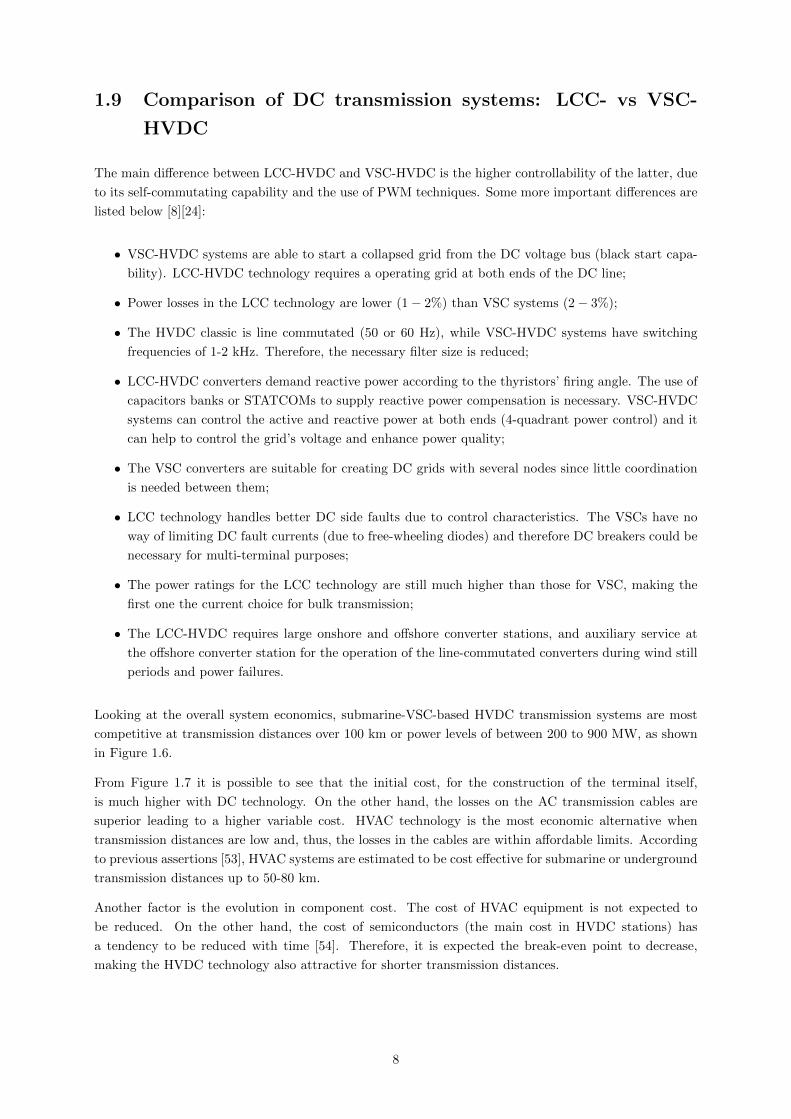
1.6 Connection technologies depending on the power and transmission distance for under-
ground or submarine cables [14]. . . . . . . . . . . . . . . . . . . . . . . . . . . . . . . . . 9
1.7 Cost Comparison between AC and DC transmission systems for underground or submarine
cables. . . . . . . . . . . . . . . . . . . . . . . . . . . . . . . . . . . . . . . . . . . . . . . . 9
1.8 Comparison between AC and DC submarine transmission cables. . . . . . . . . . . . . . . 10
1.9 Different types of offshore wind towers [15]. . . . . . . . . . . . . . . . . . . . . . . . . . . 11
1.10 Wave farm installed at Agucadoura [16]. . . . . . . . . . . . . . . . . . . . . . . . . . . . . 12
1.11 Portuguese offshore seabed’s slope. . . . . . . . . . . . . . . . . . . . . . . . . . . . . . . . 12
1.12 Portuguese offshore potential [17]. . . . . . . . . . . . . . . . . . . . . . . . . . . . . . . . 12
1.13 Possible MTDC grid in the Portuguese shore. . . . . . . . . . . . . . . . . . . . . . . . . . 12
2.1 Typical layout of a VSC-HVDC transmission system. . . . . . . . . . . . . . . . . . . . . . 13
2.2 Conventional 2-level VSC three-phase topology. . . . . . . . . . . . . . . . . . . . . . . . . 15
2.3 Main circuit of a Modular Multilevel Converter (M2C) [18]. . . . . . . . . . . . . . . . . . 16
2.4 PWM for different converter topologies. (a): two-level converter. (b): three-level converter.
(c): M2C with five modules [19]. . . . . . . . . . . . . . . . . . . . . . . . . . . . . . . . . 16
2.5 Equivalent circuit for the AC side of a VSC-HVDC station disregarding losses. . . . . . . 19
2.6 Phasor diagram of a VSC station providing active and reactive power to its AC network. 20
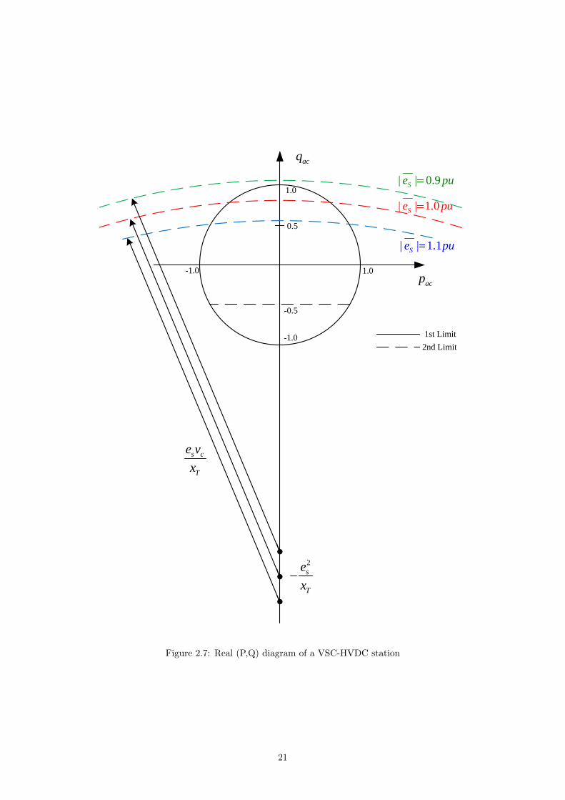
2.7 Real (P,Q) diagram of a VSC-HVDC station . . . . . . . . . . . . . . . . . . . . . . . . . 21
2.8 Equivalent circuit for AC and DC sides of a VSC-HVDC station. . . . . . . . . . . . . . . 22
2.9 VSC-HVDC Control Scheme. . . . . . . . . . . . . . . . . . . . . . . . . . . . . . . . . . . 23
viii

2.10 Block diagrams of the phase reactor and the ICC. . . . . . . . . . . . . . . . . . . . . . . 24
2.11 Active and reactive power outer controller diagrams. . . . . . . . . . . . . . . . . . . . . . 25
2.12 DC voltage controller diagram. . . . . . . . . . . . . . . . . . . . . . . . . . . . . . . . . . 26
2.13 AC Voltage outer controller diagram. . . . . . . . . . . . . . . . . . . . . . . . . . . . . . . 27
2.14 Current limiting strategies. . . . . . . . . . . . . . . . . . . . . . . . . . . . . . . . . . . . 28
3.1 MTDC Network classification scheme. . . . . . . . . . . . . . . . . . . . . . . . . . . . . . 29
3.2 Transnational “Supergrid” proposed by Airtricity [20]. . . . . . . . . . . . . . . . . . . . . 30
3.3 Wave energy in Europe in kW/m width of oncoming wave. . . . . . . . . . . . . . . . . . 32
3.4 Applications for a Multi-Terminal DC grid. . . . . . . . . . . . . . . . . . . . . . . . . . . 33
3.5 Example of a meshed-connected VSC-HVDC MTDC network with three terminals. . . . . 34
3.6 Example of a radially-connected VSC-HVDC MTDC network with four terminals. . . . . 37
4.1 MTDC grid with two DC voltage controlling stations. . . . . . . . . . . . . . . . . . . . . 46
4.2 DC voltage droop characteristic. . . . . . . . . . . . . . . . . . . . . . . . . . . . . . . . . 47
4.3 VDC(IDC) characteristics for the Droop controller - Priority Power Sharing. . . . . . . . . 48
4.4 DC voltage droop characteristics of terminals 1 and 2. . . . . . . . . . . . . . . . . . . . . 49
4.5 VDC(P ) characteristic of terminal 1 and DC voltage droop characteristic of terminal 2. . . 51
4.6 DC voltage controller and limiter present in the Voltage Margin Method. . . . . . . . . . 52
4.7 One-stage DC voltage controller. . . . . . . . . . . . . . . . . . . . . . . . . . . . . . . . . 53
4.8 VDC(P ) characteristic of the one-stage DC voltage controller. . . . . . . . . . . . . . . . . 53
4.9 VDC(P ) characteristics for two one-stage DC voltage controlling converters and the result-
ing operating point (P). . . . . . . . . . . . . . . . . . . . . . . . . . . . . . . . . . . . . . 54
4.10 Two-stage DC voltage controller. . . . . . . . . . . . . . . . . . . . . . . . . . . . . . . . . 55
4.11 VDC(P ) characteristic of a station composed by two stages. . . . . . . . . . . . . . . . . . 55
4.12 VDC(P ) characteristics for two DC voltage controlling converters and the resulting oper-
ating point (P). . . . . . . . . . . . . . . . . . . . . . . . . . . . . . . . . . . . . . . . . . . 55
4.13 VDC(P ) characteristics of the stations performing fixed power sharing. . . . . . . . . . . . 56
4.14 VDC(P ) characteristics of the stations performing priority power sharing. . . . . . . . . . 56
4.15 VDC(P ) characteristics of the stations performing proportional power sharing. . . . . . . . 56
5.1 4 terminal radial MTDC network used in the simulations. . . . . . . . . . . . . . . . . . . 58
5.2 VDC(IDC) characteristics for the droop controller - Priority Power Sharing. . . . . . . . . 60
5.3 Simulation results using the DC Voltage Droop Method - Priority Power Sharing. . . . . . 62
ix

5.4 VDC(IDC) characteristics for the Ratio controller. . . . . . . . . . . . . . . . . . . . . . . . 63
5.5 VDC(P ) characteristics for the Priority controller. . . . . . . . . . . . . . . . . . . . . . . . 64
5.6 Simulation results using the Ratio Control - Proportional Power Sharing. . . . . . . . . . 65
5.7 Simulation results using the Priority Control - Priority Power Sharing. . . . . . . . . . . . 66
5.8 VDC(P ) characteristics for the Voltage Margin Method - Fixed Power Sharing. . . . . . . 67
5.9 Simulation results using the Voltage Margin Method - Fixed Power Sharing. . . . . . . . . 68
5.10 VDC(P ) characteristics for the Voltage Margin Method - Priority Power Sharing. . . . . . 69
5.11 Simulation results using the Voltage Margin Method - Priority Power Sharing. . . . . . . 70
5.12 VDC(P ) characteristics for the Voltage Margin Method - Proportional Power Sharing. . . 71
5.13 Simulation results using the Voltage Margin Method - Proportional Power Sharing. . . . . 72
5.14 VDC(P ) characteristics for the DC voltage controllers. . . . . . . . . . . . . . . . . . . . . 73
5.15 Simulation results of a onshore three-phase AC fault. . . . . . . . . . . . . . . . . . . . . . 75
5.16 Simulation results of a onshore one-phase AC fault. . . . . . . . . . . . . . . . . . . . . . . 77
5.17 Simulation results of a offshore three-phase AC fault. . . . . . . . . . . . . . . . . . . . . . 79
6.1 Relationship between the (αβ) and (dq) frames. . . . . . . . . . . . . . . . . . . . . . . . . 90
6.2 General control scheme with saturation. . . . . . . . . . . . . . . . . . . . . . . . . . . . . 91
6.3 Anti-windup implemented: Integrator clamping. . . . . . . . . . . . . . . . . . . . . . . . 91
x

List of Acronyms
Acronym Meaning
AC Alternate Current
CFC Conversores Fonte de Corrente
CFT Conversores Fonte de Tensao
CSC Current Source Converter
DC Direct Current
EDP Energias de Portugal
GTO Gate Turn Off Thyristor
HVAC High Voltage Alternating Current
HVDC High Voltage Direct Current
ICC Inner Current Controller
IGBT Insulated Gate Bipolar Transistor
KCL Kirchhoff’s Current Law
KVL Kirchhoff’s Voltage Law
LCC Line Commutated Converter
M2C Modular Multilevel Converter
MTDC Multi-Terminal Direct Current
NSTG North Sea Transnational Grid
PCC Point of Common Coupling
PI Proportional-Integral
PID Proportional-Integral-Derivative
PLL Phase-Locked Loop
pu per unit
PWM Pulse Width Modulation
STATCOM Static Compensator
TSO Transmission System Operator
VMM Voltage Margin Method
VSC Voltage Source Converter
WF Wind Farm
XLPE Cross Linked Polyethylene
xi

List of Symbols
Symbol Meaning
αc ICC closed-loop bandwidth
αoc Outer controllers closed-loop bandwidth
δ Converter voltage phasor angle or power angle
τ DC capacitor’s time constant
ω AC system’s angular frequency
ωsw Angular switching frequency
θ Angle of the AC voltage at the PCC
(abc) Three-phase quantities frame
(αβ) Alpha-beta fixed frame
(dq) Direct-quadrature rotating frame
A State Matrix
B Input Matrix
C Station DC capacitor or Output Matrix
Ccable Capacitance of the DC cable
D Direct Transition Matrix
edq Voltage at the PCC in the (dq) frame in pu
e∗dq Reference of the voltage at the PCC in the (dq) frame in pu
|e∗dq| Magnitude reference of the voltage at the PCC in the (dq) frame in pu
es AC voltage at the PCC in pu (phasor)
ES AC voltage at the PCC (phasor)
es Magnitude of the AC voltage at the PCC in pu
f AC system’s frequency
|i| Converter’s rated current
= Imaginary axis
Iacb AC current base
IC AC current at the AC side of the converter (phasor)
Icap DC capacitor’s current
Ichopper DC chopper’s current
i∗d Reference for the d-axis of the converter’s current in pu
idc DC current at the DC side of the converter in pu
IDC DC current at the DC side of the converter
idq Current of the converter in the (dq) frame in pu
i∗dq Reference of the current of the converter in the (dq) frame in pu
IL Current flowing though a DC cable
IM Incidence Matrix
xii

IN DC cable’s nominal current
IP Active current capacity of the DC cable
i∗q Reference for the q-axis of the converter’s current in pu
i∗q,lower Current Limiter’s lower limit
i∗q,upper Current Limiter’s upper limit
k Droop of the DC voltage characteristic
Kd Derivative coefficient of a PID controller
ki Integral gain in pu
kp Proportional gain in pu
Ki,p Integral gain of the Active Power PI regulator
Ki,q Integral gain of the Reactive Power PI regulator
Ki,v Integral gain of the AC Voltage PI regulator
Ki,w Integral gain of the DC Voltage PI regulator
Kp,p Proportional gain of the Active Power PI regulator
Kp,q Proportional gain of the Reactive Power PI regulator
Kp,v Proportional gain of the AC Voltage PI regulator
Kp,w Proportional gain of the DC Voltage PI regulator
l Length of the DC cable
L Number of cables of the MTDC grid
Lcable Reactance of the DC cable
LT Total inductance between the VSC and the PCC
ma PWM modulation index
n Power ratio
N Number of nodes of the MTDC grid
P Active power
pac Active power at the AC side of the converter in pu
p∗ac Reference of the Active power at the AC side of the converter in pu
PAC Active power at the AC side of the converter
P ∗AC Active power reference
PC Active Power in the DC capacitor
PDC Active power at the DC side of the converter
Plower,1 Converter’s inversion limit of the 1-stage PI controller
Plower,2 Converter’s inversion limit of the 2-stage PI controller
Pupper,1 Converter’s rectification limit of the 1-stage PI controller
Pupper,2 Converter’s rectification limit of the 2-stage PI controller
Q Reactive power
qac Reactive power at the AC side of the converter in pu
q∗ac Reference of the Reactive power at the AC side of the converter in pu
QAC Reactive power at the AC side of the converter
Q∗AC Reactive power reference
< Real axis
R(θ) Rotation transformation matrix
Rcable Resistance of the DC cable
RT Total resistance between the VSC and the PCC
Sb Apparent Power base
Sk Short-circuit power
Sn Nominal apparent power
xiii

u∗abc Converter’s voltage reference in the (abc) frame in pu
u∗dq Converter’s voltage reference in the (dq) frame in pu
|VAC | Module of the AC voltage at the PCC
|VAC |∗ AC voltage reference
V acb AC voltage base
vc AC voltage of the converter in pu
VC AC voltage at the AC side of the converter
vc AC voltage of the converter in pu (phasor)
VC AC voltage at the AC side of the converter (phasor)
VDC DC voltage at the DC side of the converter
V ∗DC DC voltage reference
V ∗DC,H DC voltage reference of the 2-stage PI controller
w∗ DC energy reference in pu
Wb DC energy base
WC Energy stored in the DC capacitor
W ∗C DC capacitor’s energy reference
x State vector
x2 square function
xT Total reactance between the VSC and the PCC in pu
XT Total reactance between the VSC and the PCC
Z Cable impedance
xiv

Chapter 1
Introduction
1.1 Motivation
Nowadays, more than ever, there is a serious concern about the environment and the footprint made by all
sorts of humankind activities. Europe has set as goals the reduction of its primary energy consumption
and greenhouse gas emissions by 20% and to have 20% of its primary energy coming from renewable
electricity sources by 2020 [4]. At the same time the need for electric energy is increasing with time, since
it is a key component to modern societies and in developing countries is one of the most important tools
for promoting welfare and development [21].
In 2010, power plants using gas, coal or fuel oil represented 56% of all Europe’s installed power [22].
However they have two major problems: they are not renewable in the human time scale and are highly
pollutant. Moreover, countries are trying to become oil independent and, thus, there is now a strong
investment in renewable energies, such as: wind power, solar thermal, solar photovoltaic, biomass, tidal
and wave power and biofuels, among others.
One of the most utilized renewable energy sources is wind energy [22]. In Europe, onshore wind energy
technology is already a mature technology, since it has been largely installed throughout in the last years.
Indeed, the onshore wind energy market has grown in Europe in the past decade at an average pace of
33% [9], while worldwide the growth rate was of around 25%, with the total installed power reaching 159
GW in the end of 2009 [1]. However, suitable places onshore are becoming rare. Therefore, countries are
now starting to install wind turbines offshore, where space is more abundant and the wind has higher
speeds, since there are no obstacles in the open sea (see Figure 1.3).
When the distance of offshore wind farms to the shore is over 50-80 km, the electricity transmission should
be done in direct current (DC), otherwise, a large amount of the energy would be lost in the transport
itself [23][24]. Regarding DC transmission systems, there are two possible technologies: LCC-HVDC
(HVDC classic) or VSC-HVDC technology.
The VSC-HVDC technology has a higher control capability when compared with the classic alternative,
since it can independently control the active and the reactive power exchanged with the connected AC
network. Additionally, the footprint of a VSC station is smaller, since the filters needed are smaller - due
to the use of PWM techniques - and this is a key factor, since building large structures offshore tends
to be expensive. Furthermore, with VSCs there is no need for reactive power compensation and the
necessary communication between stations is smaller making this technology more attractive for offshore
purposes [25][26].
1

1.2 Thesis objective and contributions
One of the main purposes of this thesis is to model VSC-HVDC systems for dynamic simulation analysis
of multi-terminal direct current (MTDC) networks. In fact, the proposed models are independent of the
DC grid configuration, and therefore, they can be used to simulate any multi-terminal system. The model
of MTDC networks is also concerned in this thesis.
Another major contribution is the comparison of several DC voltage control methods for VSC-HVDC
stations inside MTDC networks. The following methods will be studied: Voltage Droop Method, Priority
Control, Ratio Control, and Voltage Margin Method. They will be compared in terms of steady-state
and dynamic behavior, expansibility, flexibility, reliability, controllability, and fault handling capability.
In the present work all the equivalent models are implemented in the MATLAB/Simulink software in
order to represent, as realistically as possible, the entire MTDC transmission system.
1.3 Publications
The present thesis has resulted in the following publications:
• R. Teixeira Pinto, S. F. Rodrigues, P. Bauer, J. Pierik: Comparison of Direct Voltage Control
Methods of Multi-Terminal DC (MTDC) Networks through Modular Dynamic Models; European
Power Electronics Conference 2011; 30 August - 01 September, Birmingham.
• R. Teixeira Pinto, S. F. Rodrigues, P. Bauer, J. Pierik: Description and Comparison of DC Voltage
Control Strategies for Offshore MTDC Networks: Steady-State and Fault Analysis; Submitted to
European Power Electronics Journal.
• P. D. Chainho, S. F. Rodrigues, A. van der Meer, R. Teixeira Pinto, “Dynamic model of Multiter-
minal DC grids through State-Space Representation,” 2011.
1.4 Thesis layout
This thesis is structured in six chapters. In Chapter 1, an introduction to the current status of the
offshore wind energy is made. An overview on the existing wind energy capacity and its distribution in
Europe is done. A comparison between transmission systems, HVDC (LCC and VSC) and HVAC, is
made. In Chapter 2, a typical VSC-HVDC station is presented and a description about its components is
done. Further on, the VSC equivalent model and its controllers are explained in detail. In Chapter 3, the
MTDC grid is modeled and its characteristics are described. The different DC voltage control methods
implemented are described and explained in Chapter 4. In Chapter 5, simulations are carried out and
the results are shown and interpreted. In Chapter 6, conclusions and recommendations for future work
are presented.
2
1.5 State of the Art
In order to build an offshore electrical power transmission system there are three different possibilities
available: HVAC, LCC-HVDC and VSC-HVDC. Comparisons between these transmission technologies
regarding power efficiency and economical aspects can be found in the literature [6][8][26][27][28]. The
cost of submarine transmission systems for the different technologies can be found at [24].
Recent advances in HVDC power transmission systems and a list of projects that make use of the VSC
technology can be found at [29]. The VSC multilevel (M2C) is explained in detail at [30], while the study
and development of its model is presented at [31].
Different VSC topologies and the description of the components normally present in a VSC transmission
system can be found in the literature at [32][33]. The AC and DC models of the VSC are achieved and
implemented in [19][34]. The inner current controller and the outer controllers for the VSC technology
are described in the previous references of the present paragraph and also at [25][35]. The capability
curve of a VSC is explained in detail at [36].
Information about anti-wind up strategies, e.g. back-calculation and conditional integration, is possible
to be found at [37][38].
The need for MTDC grids and their applications can be found in the literature at [39]. The use of
State-Space Models to derive a model of a VSC and a point-to-point transmission system is presented at
[40]. The model of a MTDC grid, also making use of State-Space Model, is achieved at [41].
Several DC voltage control methods have been presented in the literature. The Ratio Control and the
Priority Control can be found at [42]. The Priority Control strategy and its behavior when a wind farm
is lost is presented at [43]. The Voltage Droop is explained at [44]. The Voltage Margin method with
2 DC voltage stages is presented and explained in detail at [45][46]. A 3-stage VMM and its dynamic
response when a onshore station is disconnected from the MTDC grid is described at [34].
Models of DC choppers are presented and described in [34][47]. Fault Ride Through methods are presented
in the literature at [48][49]. The study about AC faults and its consequences can be found at [19][33][34].
3
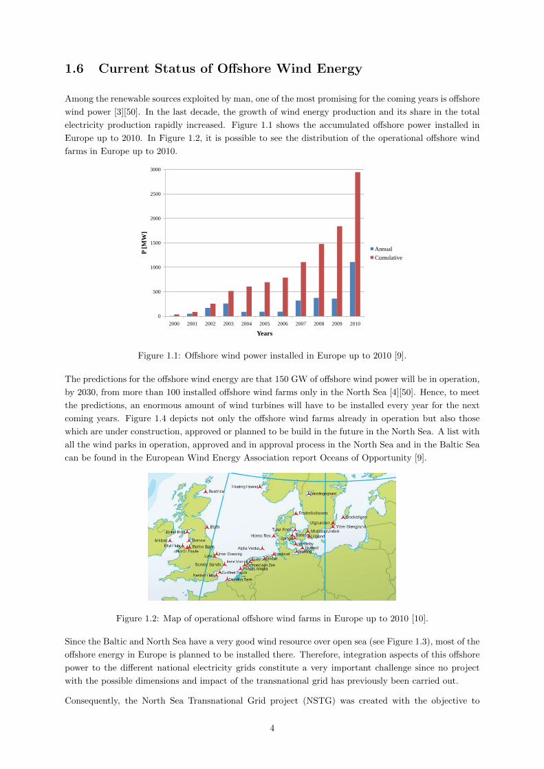
1.6 Current Status of Offshore Wind Energy
Among the renewable sources exploited by man, one of the most promising for the coming years is offshore
wind power [3][50]. In the last decade, the growth of wind energy production and its share in the total
electricity production rapidly increased. Figure 1.1 shows the accumulated offshore power installed in
Europe up to 2010. In Figure 1.2, it is possible to see the distribution of the operational offshore wind
farms in Europe up to 2010.
0
500
1000
1500
2000
2500
3000
2000 2001 2002 2003 2004 2005 2006 2007 2008 2009 2010
P [
MW
]
Years
Annual
Cumulative
Figure 1.1: Offshore wind power installed in Europe up to 2010 [9].
The predictions for the offshore wind energy are that 150 GW of offshore wind power will be in operation,
by 2030, from more than 100 installed offshore wind farms only in the North Sea [4][50]. Hence, to meet
the predictions, an enormous amount of wind turbines will have to be installed every year for the next
coming years. Figure 1.4 depicts not only the offshore wind farms already in operation but also those
which are under construction, approved or planned to be build in the future in the North Sea. A list with
all the wind parks in operation, approved and in approval process in the North Sea and in the Baltic Sea
can be found in the European Wind Energy Association report Oceans of Opportunity [9].
Figure 1.2: Map of operational offshore wind farms in Europe up to 2010 [10].
Since the Baltic and North Sea have a very good wind resource over open sea (see Figure 1.3), most of the
offshore energy in Europe is planned to be installed there. Therefore, integration aspects of this offshore
power to the different national electricity grids constitute a very important challenge since no project
with the possible dimensions and impact of the transnational grid has previously been carried out.
Consequently, the North Sea Transnational Grid project (NSTG) was created with the objective to
4

Figure 1.3: European wind resources over open sea[11].
Figure 1.4: Actual and future planned offshore windfarms in the North Sea [3].
identify and study the technical and economic aspects with regard to the development of a transnational
electricity network in the North Sea for the connection of offshore wind power and trade between European
countries [4].
1.7 Offshore Transmission technologies
One of the challenges is to find the most suitable technology to connect the offshore wind farms to shore,
having different power ratings and different distances from the onshore connection point. This selection
should be done by taking into consideration power efficiency and economical aspects. In order to build
an offshore electrical power transmission system there are three different possibilities available: HVAC,
LCC-HVDC and VSC-HVDC. In this section these three technologies are going to be present, explained
and compared.
1.7.1 HVAC
Most of the existing offshore transmission systems use HVAC for the transport of electrical power between
mainland and stations located offshore. The reasons for choosing this technology are: lower station costs,
no power converters needed, and a simpler layout for the offshore wind farm is possible. HVAC systems
contain the following main components: an AC collecting system in the platform, an offshore transforming
substation with transformers and reactive power compensation, three-phase submarine cable (generally
XLPE three-core cable) and an onshore transforming substation with transformers and reactive power
compensation.
Depending on the distance to the connection point and on the power that has to be transmitted, there
are different solutions that can be engaged. For a shorter distance and smaller power a direct connection
5
over middle voltage can be used and therefore, collecting transformer and high voltage transmission can
be avoided. For a higher power or a longer distance the use of high voltage for transmission and collecting
transformers is inevitable. When the voltage of the transmission cable and the grid voltage are equal the
onshore transformer is not necessary.
Due to their construction, distributed capacitance in submarine cables is much higher than in overhead
lines. This implies that the maximum feasible length and power transmission capacity of HVAC cables is
limited. The reactive power that is inherently generated in HVAC cables increases with both the square
of the voltage level and the cable length. Thus, for distant transmission distances and high voltage levels,
reactive power compensation will be required at both cable ends.
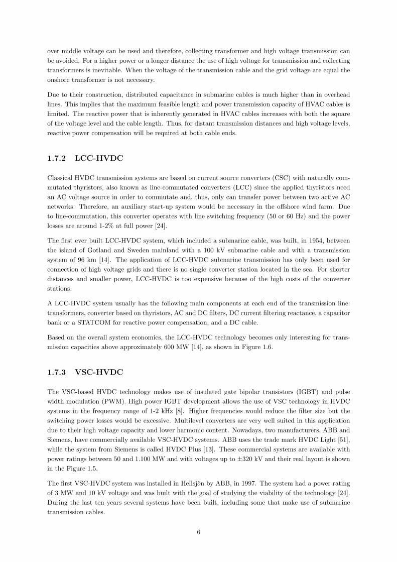
1.7.2 LCC-HVDC
Classical HVDC transmission systems are based on current source converters (CSC) with naturally com-
mutated thyristors, also known as line-commutated converters (LCC) since the applied thyristors need
an AC voltage source in order to commutate and, thus, only can transfer power between two active AC
networks. Therefore, an auxiliary start-up system would be necessary in the offshore wind farm. Due
to line-commutation, this converter operates with line switching frequency (50 or 60 Hz) and the power
losses are around 1-2% at full power [24].
The first ever built LCC-HVDC system, which included a submarine cable, was built, in 1954, between
the island of Gotland and Sweden mainland with a 100 kV submarine cable and with a transmission
system of 96 km [14]. The application of LCC-HVDC submarine transmission has only been used for
connection of high voltage grids and there is no single converter station located in the sea. For shorter
distances and smaller power, LCC-HVDC is too expensive because of the high costs of the converter
stations.
A LCC-HVDC system usually has the following main components at each end of the transmission line:
transformers, converter based on thyristors, AC and DC filters, DC current filtering reactance, a capacitor
bank or a STATCOM for reactive power compensation, and a DC cable.
Based on the overall system economics, the LCC-HVDC technology becomes only interesting for trans-
mission capacities above approximately 600 MW [14], as shown in Figure 1.6.
1.7.3 VSC-HVDC
The VSC-based HVDC technology makes use of insulated gate bipolar transistors (IGBT) and pulse
width modulation (PWM). High power IGBT development allows the use of VSC technology in HVDC
systems in the frequency range of 1-2 kHz [8]. Higher frequencies would reduce the filter size but the
switching power losses would be excessive. Multilevel converters are very well suited in this application
due to their high voltage capacity and lower harmonic content. Nowadays, two manufacturers, ABB and
Siemens, have commercially available VSC-HVDC systems. ABB uses the trade mark HVDC Light [51],
while the system from Siemens is called HVDC Plus [13]. These commercial systems are available with
power ratings between 50 and 1.100 MW and with voltages up to ±320 kV and their real layout is shown
in the Figure 1.5.
The first VSC-HVDC system was installed in Hellsjon by ABB, in 1997. The system had a power rating
of 3 MW and 10 kV voltage and was built with the goal of studying the viability of the technology [24].
During the last ten years several systems have been built, including some that make use of submarine
transmission cables.
6

Figure 1.5: Layout of a real VSC-HVDC station: ABB HVDC Light and SIEMENS HVDC Plus, respec-tively [12][13].
A VSC-HVDC system has the following main components: AC breakers, AC filters, a transformer, a
phase reactor, a voltage source converter, a DC capacitor, and a DC cable to connect it to another
station or grid.
1.8 Comparison of transmission systems: HVAC vs HVDC
HVAC systems are widely used and have lower costs than the HVDC technology in underground or
submarine short-transmission distances (distances up to 50-80 km, although this distance may be re-
duced soon). A major drawback of HVAC systems is the limited transmission distance. On the other
hand, HVDC technology have no practical transmission distance limitation and needs less cabling than
equivalent HVAC, generating a considerable cable and installation cost reduction, and the maintenance,
environmental impact and fault rate are also reduced. HVDC technology (either LCC or VSC) has many
technical advantages when compared to HVAC technology which can be very important if the contribu-
tion of offshore power generation is expected to be a major player in the electrical energy generation and
the grid stability. These advantages are [26][52]:
• The losses in a DC cable are lower than in an AC cable for long distances;
• Asynchronous connections of the offshore farms and the onshore grids are only possible with HVDC
technology. The frequency and phase of both transmitting ends do not have to be synchronized
because the DC link decouples them. Grid voltage dips and other faults do not have a direct effect
in the generators of the offshore farm, and therefore, there is a higher flexibility in the design of
these units;
• HVDC technology allows almost instantaneous control over the transmitted power and the system
can contribute to the frequency control of the grid;
• The VSC-HVDC technology can control active and reactive power independently. Thus, it is
possible to control both AC and DC voltages of the converter. This feature is very helpful if the
connected grid is weak;
• Unlike HVAC, the HVDC technology does not increase the short-circuit level of the connected AC
system.
7
1.9 Comparison of DC transmission systems: LCC- vs VSC-
HVDC
The main difference between LCC-HVDC and VSC-HVDC is the higher controllability of the latter, due
to its self-commutating capability and the use of PWM techniques. Some more important differences are
listed below [8][24]:
• VSC-HVDC systems are able to start a collapsed grid from the DC voltage bus (black start capa-
bility). LCC-HVDC technology requires a operating grid at both ends of the DC line;
• Power losses in the LCC technology are lower (1− 2%) than VSC systems (2− 3%);
• The HVDC classic is line commutated (50 or 60 Hz), while VSC-HVDC systems have switching
frequencies of 1-2 kHz. Therefore, the necessary filter size is reduced;
• LCC-HVDC converters demand reactive power according to the thyristors’ firing angle. The use of
capacitors banks or STATCOMs to supply reactive power compensation is necessary. VSC-HVDC
systems can control the active and reactive power at both ends (4-quadrant power control) and it
can help to control the grid’s voltage and enhance power quality;
• The VSC converters are suitable for creating DC grids with several nodes since little coordination
is needed between them;
• LCC technology handles better DC side faults due to control characteristics. The VSCs have no
way of limiting DC fault currents (due to free-wheeling diodes) and therefore DC breakers could be
necessary for multi-terminal purposes;
• The power ratings for the LCC technology are still much higher than those for VSC, making the
first one the current choice for bulk transmission;
• The LCC-HVDC requires large onshore and offshore converter stations, and auxiliary service at
the offshore converter station for the operation of the line-commutated converters during wind still
periods and power failures.
Looking at the overall system economics, submarine-VSC-based HVDC transmission systems are most
competitive at transmission distances over 100 km or power levels of between 200 to 900 MW, as shown
in Figure 1.6.
From Figure 1.7 it is possible to see that the initial cost, for the construction of the terminal itself,
is much higher with DC technology. On the other hand, the losses on the AC transmission cables are
superior leading to a higher variable cost. HVAC technology is the most economic alternative when
transmission distances are low and, thus, the losses in the cables are within affordable limits. According
to previous assertions [53], HVAC systems are estimated to be cost effective for submarine or underground
transmission distances up to 50-80 km.
Another factor is the evolution in component cost. The cost of HVAC equipment is not expected to
be reduced. On the other hand, the cost of semiconductors (the main cost in HVDC stations) has
a tendency to be reduced with time [54]. Therefore, it is expected the break-even point to decrease,
making the HVDC technology also attractive for shorter transmission distances.
8
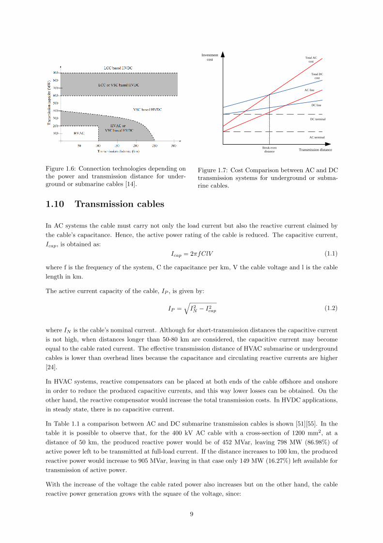
Figure 1.6: Connection technologies depending onthe power and transmission distance for under-ground or submarine cables [14].
Transmission distance
Investment
costTotal AC
cost
Total DC
cost
AC terminal
DC terminal
DC line
AC line
Break-even
distance
Figure 1.7: Cost Comparison between AC and DCtransmission systems for underground or subma-rine cables.
1.10 Transmission cables
In AC systems the cable must carry not only the load current but also the reactive current claimed by
the cable’s capacitance. Hence, the active power rating of the cable is reduced. The capacitive current,
Icap, is obtained as:
Icap = 2πfClV (1.1)
where f is the frequency of the system, C the capacitance per km, V the cable voltage and l is the cable
length in km.
The active current capacity of the cable, IP , is given by:
IP =√I2N − I2cap (1.2)
where IN is the cable’s nominal current. Although for short-transmission distances the capacitive current
is not high, when distances longer than 50-80 km are considered, the capacitive current may become
equal to the cable rated current. The effective transmission distance of HVAC submarine or underground
cables is lower than overhead lines because the capacitance and circulating reactive currents are higher
[24].
In HVAC systems, reactive compensators can be placed at both ends of the cable offshore and onshore
in order to reduce the produced capacitive currents, and this way lower losses can be obtained. On the
other hand, the reactive compensator would increase the total transmission costs. In HVDC applications,
in steady state, there is no capacitive current.
In Table 1.1 a comparison between AC and DC submarine transmission cables is shown [51][55]. In the
table it is possible to observe that, for the 400 kV AC cable with a cross-section of 1200 mm2, at a
distance of 50 km, the produced reactive power would be of 452 MVar, leaving 798 MW (86.98%) of
active power left to be transmitted at full-load current. If the distance increases to 100 km, the produced
reactive power would increase to 905 MVar, leaving in that case only 149 MW (16.27%) left available for
transmission of active power.
With the increase of the voltage the cable rated power also increases but on the other hand, the cable
reactive power generation grows with the square of the voltage, since:
9
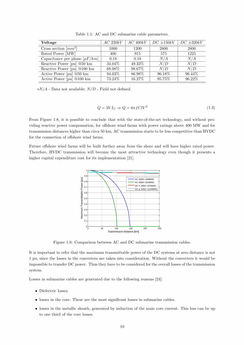
Table 1.1: AC and DC submarine cable parameters.
Voltage AC 220kV AC 400kV DC ±150kV DC ±320kV
Cross section [mm2] 1000 1200 2800 2800Rated Power [MW] 400 915 575 1225Capacitance per phase [µF/km] 0.18 0.18 N/A N/AReactive Power [pu] @50 km 34.04% 49.33% N/D N/DReactive Power [pu] @100 km 68.08% 98.67% N/D N/DActive Power [pu] @50 km 94.03% 86.98% 96.18% 96.44%Active Power [pu] @100 km 73.24% 16.27% 95.75% 96.22%
∗N/A - Data not available; N/D - Field not defined.
Q = 3V IC ⇒ Q = 6πfClV 2 (1.3)
From Figure 1.8, it is possible to conclude that with the state-of-the-art technology, and without pro-
viding reactive power compensation, for offshore wind farms with power ratings above 400 MW and for
transmission distances higher than circa 50 km, AC transmission starts to be less competitive than HVDC
for the connection of offshore wind farms.
Future offshore wind farms will be built further away from the shore and will have higher rated power.
Therefore, HVDC transmission will become the most attractive technology even though it presents a
higher capital expenditure cost for its implementation [21].
0 50 100 150 200 2500
0.1
0.2
0.3
0.4
0.5
0.6
0.7
0.8
0.9
1
Transmission distance [km]
Ma
xim
um
Tra
nsm
itta
ble
Po
we
r [p
u]
AC 220kV (400MW)
AC 400kV (915MW)
DC 150kV (575MW)
DC 320kV (1225MW)
Figure 1.8: Comparison between AC and DC submarine transmission cables.
It is important to refer that the maximum transmittable power of the DC systems at zero distance is not
1 pu, since the losses in the converters are taken into consideration. Without the converters it would be
impossible to transfer DC power. Thus they have to be considered for the overall losses of the transmission
system.
Losses in submarine cables are generated due to the following reasons [24]:
• Dielectric losses.
• losses in the core. These are the most significant losses in submarine cables.
• losses in the metallic sheath, generated by induction of the main core current. This loss can be up
to one third of the core losses.
10
• losses in the steel armature, also generated by induction of the main core current. This loss can be
up to one third of the core losses as well.
1.11 Wind Energy in Portugal
Portugal in terms of electricity’s percentage that comes from wind farms is, nowadays, only surpassed
by Denmark. The electricity that comes from this energy source is 14.8% of all the electricity consumed.
At the end of 2010, there were about 4 GW of onshore wind energy capacity installed in Portugal - all
onshore. By 2020, Portugal aims to have around 7 GW of wind energy capacity, providing 23% of all the
electricity needed.
The power grid is a limiting factor for many countries, but is a particularly problem for Portugal given
its position on the periphery of Europe. The Iberian Peninsula is notoriously poorly linked to the rest of
Europe. This means that nearly all the power produced in Portugal stays there.
Portugal has plenty of onshore wind energy installed but none offshore. The major reason for this are
the geographical characteristics of the Atlantic Ocean which, unlike Europe’s northern waters, becomes
deep extremely quickly. This makes it difficult to put up today’s standard offshore wind turbines, whose
foundations rest on the seabed. Another difficulty is that, on average, the wave height on the Atlantic
ocean is twice that of the North Sea [56].
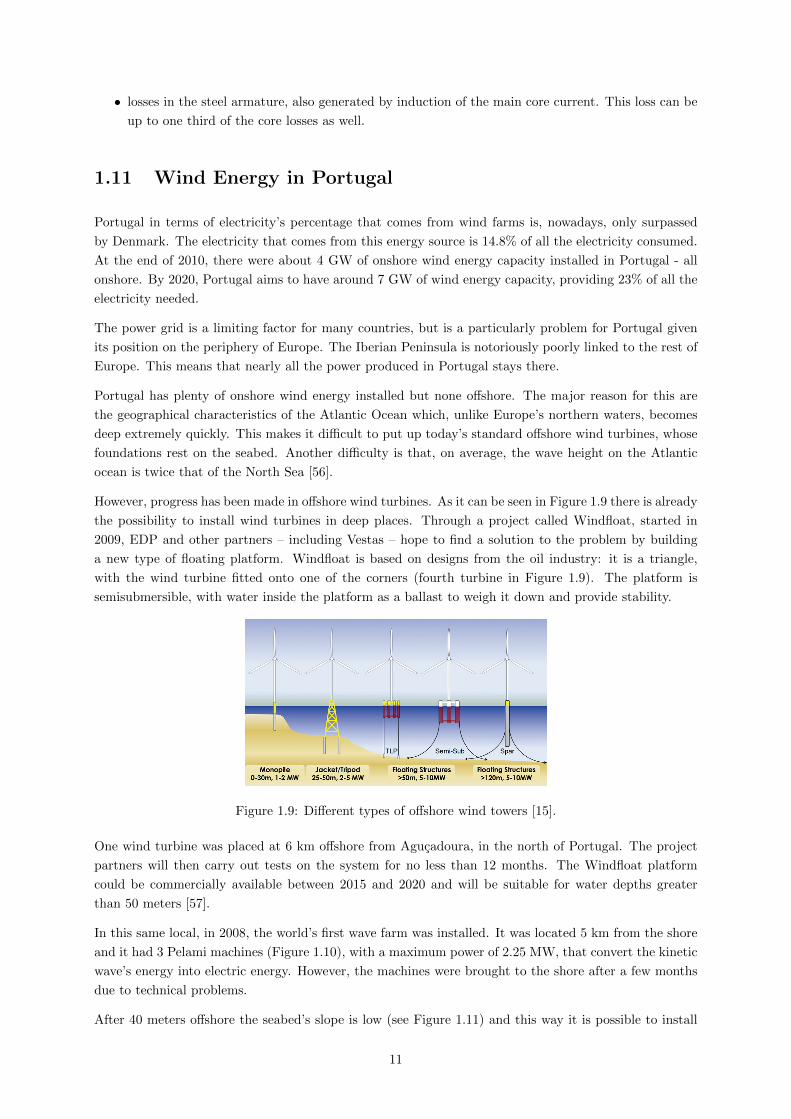
However, progress has been made in offshore wind turbines. As it can be seen in Figure 1.9 there is already
the possibility to install wind turbines in deep places. Through a project called Windfloat, started in
2009, EDP and other partners – including Vestas – hope to find a solution to the problem by building
a new type of floating platform. Windfloat is based on designs from the oil industry: it is a triangle,
with the wind turbine fitted onto one of the corners (fourth turbine in Figure 1.9). The platform is
semisubmersible, with water inside the platform as a ballast to weigh it down and provide stability.
Figure 1.9: Different types of offshore wind towers [15].
One wind turbine was placed at 6 km offshore from Agucadoura, in the north of Portugal. The project
partners will then carry out tests on the system for no less than 12 months. The Windfloat platform
could be commercially available between 2015 and 2020 and will be suitable for water depths greater
than 50 meters [57].
In this same local, in 2008, the world’s first wave farm was installed. It was located 5 km from the shore
and it had 3 Pelami machines (Figure 1.10), with a maximum power of 2.25 MW, that convert the kinetic
wave’s energy into electric energy. However, the machines were brought to the shore after a few months
due to technical problems.
After 40 meters offshore the seabed’s slope is low (see Figure 1.11) and this way it is possible to install
11

500 MW of offshore wind power in the north of Portugal and 700 MW more in the center [17]. The
productivity could reach 3400 hours per year as it can be seen in Figure 1.12.
Figure 1.10: Wave farm installed at Agucadoura [16]. Figure 1.11: Portuguese offshore seabed’s slope.
In Figure 1.13 it is shown a possible MTDC grid installation for the Portuguese shore. With this grid it
would be possible to connect all the Portuguese offshore wind farms and also the wave farms, if available.
Figure 1.12: Portuguese offshore potential [17].
180km
Figure 1.13: Possible MTDC grid in the Portugueseshore.
12
Chapter 2
VSC-HVDC Equivalent Model and
Controllers
2.1 Introduction
The main objective of the present chapter is to achieve an equivalent model of a VSC-HVDC station and
its control system. Firstly, the components of a typical VSC-HVDC transmission system are presented
and described. Further on, the equivalent models of the AC and DC sides of the VSC station are derived.
In the last part of the chapter the entire control system is presented and explained.
2.2 VSC-HVDC Transmission System
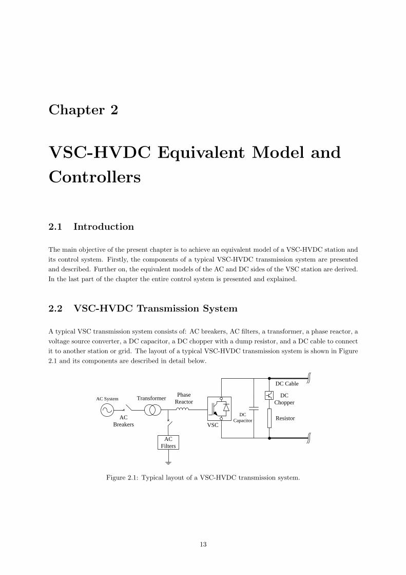
A typical VSC transmission system consists of: AC breakers, AC filters, a transformer, a phase reactor, a
voltage source converter, a DC capacitor, a DC chopper with a dump resistor, and a DC cable to connect
it to another station or grid. The layout of a typical VSC-HVDC transmission system is shown in Figure
2.1 and its components are described in detail below.
AC System
DC Cable
DC
Capacitor
Phase
Reactor
AC
Filters
Transformer
AC
Breakers VSC
Resistor
DC
Chopper
Figure 2.1: Typical layout of a VSC-HVDC transmission system.
13
2.2.1 AC Breakers
The presence of an AC circuit breaker (located in the AC switchyard) is needed in a VSC-HVDC station
due to several reasons [32]:
• to have the ability of disconnecting the station from the AC system for maintenance;
• to connect the AC system to the VSC link when the DC capacitor needs to be charged at the
start-up of the VSC-HVDC transmission system;
• to disconnect the VSC link from the AC system during DC-side fault, since differently from the
HVDC classic (LCC-HVDC), the 2- or 3-level VSC transmission system has no mechanism to clear
DC-side faults.
2.2.2 AC Filters
The presence of harmonics in the VSC-HVDC system may be very prejudicial to the transmission system
and to the connected AC network. Some phenomena that may occur due to the presence of harmonics
are:
• Higher losses and overheating in the system;
• Over-voltages, due to the existence of resonance;
• Interference, inaccuracy or instability in the control systems;
• Noise on voice-frequency telephone lines and radio.
Because of all the phenomena above, the presence of AC filters is important. Nevertheless, PWM opera-
tion reduces significantly the harmonic content. Therefore, AC filters in a VSC link will be smaller and
cheaper than in HVDC classic.
The AC filter acts as a high-pass filter, tuned so that the high-frequency signals are given an easier
path to earth (lower resistance). The filter is installed between the transformer and the converter and
it prevents harmonics from entering the AC system, and filters high-frequency components so that the
transformer is not exposed to high-frequency stress. Additionally, sinusoidal currents and voltages can
be obtained at the secondary side of the transformer due to the presence of the AC filters.
The design of the filter is, in most of the cases, made for the AC grid that is going to be connect to the
VSC station. For this reason it is necessary to know the AC network impedance seen from the connection
point. However, this information is difficult to be obtained and usually project related [33][58].
2.2.3 Transformer
The converters are connected to the AC system, in most cases, via transformers. The most important
function of the transformers is to change the voltage of the AC network to a voltage level that is appro-
priate for the converter. The transformer also acts as a galvanic barrier between AC and DC sides. This
is important since some faults in the AC system give overvoltages in the healthy phases. Furthermore,
the reactance of the transformer will reduce short circuit currents.
Standard two-winding transformers can be used since for VSC-HVDC applications since there is no need
to block DC components. The transformer can be represented by a combination of a π equivalent and
an ideal transformer. Alternatively, it can be represented simply by its leakage reactance.
14

2.2.4 Phase Reactor
The phase reactor is one of the most important elements installed on the AC side of the VSC station. The
phase reactor has several purposes: it reduces the high-frequency harmonic content of the AC current (it
acts as a low-pass filter), prevents changes in the current polarity in the IGBT valves (due to switching).
Additionally, it allows to control active and reactive power independently by adjusting the current that
flows through it and it also limits the short-circuit currents. Usually the chosen value to the phase reactor
impedance is kept between 0.10-0.25 pu and is selected as a compromise between harmonic attenuation
and voltage droop on the reactance [51].
2.2.5 Voltage Source Converter
Voltage source converters employ self-commutating switches, e.g., gate turn off thyristors (GTOs) or
IGBTs, which can be turned on or off freely. Therefore, a VSC can produce its own sinusoidal voltage
waveform using PWM technology independent of the interconnected AC system.
The 2-level bridge is the simplest topology (see Figure 2.2) that can be used in order to build up a
three-phase forced-commutated VSC bridge. The bridge consists of six valves and each valve consists of
a self-commutating switch device and an anti-parallel diode.
Figure 2.2: Conventional 2-level VSC three-phase topology.
The operation principle of the 2-level bridge is simple. Each phase of the VSC can be connected either to
the positive or the negative DC terminal. By adjusting the width of the pulses, the reference voltage can
be reproduced, as shown in Figure 2.4 (a). AC filters are mandatory for reducing the harmonic content
due to the switching operation of the IGBTs in order to prevent disturbances in the AC system.
Almost all the VSC-HVDC transmission systems implemented so far employ 2- or 3-level (Figure 2.4
(b)) PWM converters. However, some years ago, an alternative VSC-HVDC, commonly referred to as
Modular Multilevel Converter (M2C), was suggested [31]. This solution is based on series-connection of
sub-modules containing a semiconductor half-bridge and a DC capacitor (see Figure 2.3). Siemens was
the first company to win an order of an HVDC link using M2C technology. The Trans Bay HVDC Link
in the San Francisco area entered into operation in 2010. The HVDC link is rated at ± 200 kV and the
rated power is 400 MW [59].
Each arm of the VSC is composed of a series-connection of sub-modules. The function of the half-bridge
is to insert or bypass the sub-module capacitor in the chain of series-connected sub-modules. The control
system keeps the average of the sum of the number of inserted sub-modules in the upper and the lower
arm at a constant level in order to balance the applied DC voltage. The AC voltage is obtained by
changing the number of inserted sub-modules in the upper and the lower arms.
15
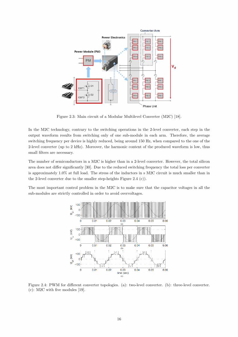
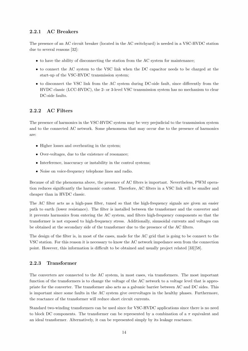
Figure 2.3: Main circuit of a Modular Multilevel Converter (M2C) [18].
In the M2C technology, contrary to the switching operations in the 2-level converter, each step in the
output waveform results from switching only of one sub-module in each arm. Therefore, the average
switching frequency per device is highly reduced, being around 150 Hz, when compared to the one of the
2-level converter (up to 2 kHz). Moreover, the harmonic content of the produced waveform is low, thus
small filters are necessary.
The number of semiconductors in a M2C is higher than in a 2-level converter. However, the total silicon
area does not differ significantly [30]. Due to the reduced switching frequency the total loss per converter
is approximately 1.0% at full load. The stress of the inductors in s M2C circuit is much smaller than in
the 2-level converter due to the smaller step-heights Figure 2.4 (c)).
The most important control problem in the M2C is to make sure that the capacitor voltages in all the
sub-modules are strictly controlled in order to avoid overvoltages.
(a)
(b)
(c)
Figure 2.4: PWM for different converter topologies. (a): two-level converter. (b): three-level converter.(c): M2C with five modules [19].
16

2.2.6 DC Capacitor
The DC capacitor is one of the most important elements in a VSC transmission system and usually is
placed inside the converter station. The DC capacitor acts as a DC voltage source since it helps to keep
the DC voltage constant within close limits. By increasing the DC capacitor’s size the transient response
is enhanced, and the DC voltage stiffness and control bandwidth are increased. However, it is expensive
to augment the size of the capacitor.
The design of the DC capacitor has to be carefully carried out due to its importance in a HVDC system.
Because of the PWM switching action in the VSC-HVDC, the current flowing to the DC side of the
converter contains harmonics which will result in a ripple on the DC side voltage. Since large power
imbalances may occur during disturbances between the AC and DC side, such as faults or switching
maneuvers while changing the operating point, the size of the capacitor cannot be only determined
by steady-state operation because that would lead to DC over-voltages that may stress or damage the
converter’s valves. So it is extremely important to take into consideration the transient voltage constrain
when the DC capacitor is to be chosen [32].
A time constant, τ , characterizes the DC capacitor and it is defined as the ratio between the energy stored
in the capacitor when the nominal DC voltage, VDC , is applied to the converter at nominal apparent
power (Sn):
τ =1
2CVDC
2
Sn[s] (2.1)
The time constant, τ , defines the time that is necessary to completely charge the DC capacitor (starting
with from zero DC voltage) at nominal power.
2.2.7 DC Cable
The cable used in the VSC-HVDC applications can be designed to use extruded polymeric insulation,
which is particularly resistant to the DC voltage, as a substitute to the conventional oil-impregnated
paper insulation.
AC XLPE cables cannot be directly used for DC transmission due to a phenomenon called space charges.
The DC voltage creates an electric field, which would cause space charges to move and accumulate in
certain spots of the insulation, resulting in its degradation. Special XLPE cables have been developed
in order to prevent space charge problems to happen. A precondition for such cables is that the voltage
polarity does not change rapidly, as this causes high stresses in the insulation. Since in the VSC-HVDC
power flow reversal does not require the inversion of the DC voltage polarity, XLPE cables can be used.
This results in lighter and more flexible cables with no risk of oil leakage, since the insulator is solid, and
the installation of these cables is easier and faster. A special type of XLPE cables are submarine cables,
which face harsh environmental conditions and because of that they are armored with galvanized steel
wire for mechanical sturdiness [58].
All VSC-HVDC systems in operation are equipped with XLPE cables. Cables with voltages up to ± 320
kV DC are presently available [51].
The risk of a DC fault is reduced when using cables. This is an important aspect since no DC breakers are
present in VSC-HVDC systems as previously explained. The conductors for HVDC transmission system
can be modeled by a π circuit, which is sufficiently accurate for short to middle-long distances.
17
2.2.8 DC Chopper
The DC chopper consists of voltage-triggered power electronic switches and resistors. When the DC
voltage rises above a predefined threshold value, the power electronic components start switching and
part of the DC current is dissipated in the resistors. The amount of current dissipated depends on the
duty ratio of the switches and therefore, it depends on the value of the DC voltage. The amount of power
dissipated is, however, limited to the rated capacity of the DC chopper [47].
During an onshore fault, the onshore stations are unable to deliver active power to the onshore grid,
which causes the DC voltage to increase due to the power imbalance. Therefore, the active power being
transmitted from the offshore wind farms has to be reduced. The DC chopper requires a simple control
and can be triggered directly by using a hysteresis function based on the DC voltage. The main advantage
of this technique is that the wind farms stay unaffected by the fault i.e., the output power of the wind
farms remain constant during the fault. Moreover, there is no impact on the mechanical drive train and
thus, the wind farms do not speed up during the fault [49].
2.3 Voltage Source Converter’s equivalent model
2.3.1 Equivalent model of the VSC AC side
It is possible to consider the AC side of a VSC-HVDC station as a controllable voltage source since
a converter using PWM techniques is able to control independently the frequency, the phase and the
amplitude of its AC voltage. This voltage source can be described as:
VC(t) =√
2 · VC · sin(ωt+ δ) + harmonics with VC = ma ·VDC
2(2.2)
where ma stands for the PWM modulation index, w is the angular frequency of the voltage fundamental
component, and δ is the phase angle difference between the AC network and the converter fundamental
voltage [60].
In a VSC-HVDC station, as discussed in section 2.2, a phase reactor, AC filters and a transformer are
usually present. Thus, it is possible to disregard the switching harmonics, and assume that the voltage
of the converter is equal to the modulator (PWM) reference voltage, as long as the modulator reference
voltage does not exceed the linear region [61].
The equivalent diagram of a VSC link connected to an AC system is shown in Figure 2.5. As shown
in the figure, the AC system and the controllable voltage source are connected via series reactors (XT ),
since the transformer and the phase reactor resistances can be neglected when compared to the sum of
the inductive reactances. The AC voltages represented in Figure 2.5 are line voltages: ES = ESej0 and
VC = VCejδ.
If the transformer and reactor resistances are disregarded (i.e. lossless), the active power flow between
the AC network and the VSC can be formulated, in pu, as [29][51]:
pac =esvcxT
sin(δ) (2.3)
From the above equation it is possible to realize that the control of the active power flow is accomplished
by changing the VSC voltage output phase angle, δ, while maintaining all the other variables unchanged.
18

TX
CVSE
CI,AC ACP Q
Figure 2.5: Equivalent circuit for the AC side of a VSC-HVDC station disregarding losses.
This is achieved through PWM technique by controlling the switching instant of the converter’s valves.
δ < 0 ⇒ vc lagging es ⇒ pac < 0 (Invertion)
δ > 0 ⇒ vc leading es ⇒ pac > 0 (Rectification)(2.4)
If the voltages of the AC network of the VSC are in phase, i.e. δ = 0, there will be no transfer of active
power (disregarding losses) and the VSC will operate as a reactive power compensator, absorbing or
providing reactive power as needed. Under such cases the VSC operates as a STATCOM [5].
The reactive power flow between the AC network and the VSC station can be calculated as [29][51]:
qac =esxT
(es − vc cos(δ)) (2.5)
From the equation (2.5) it is possible to observe that if the real component of the VSC output voltage
(vccos(δ)) has a smaller magnitude than the voltage of the AC system, the converter will consume reactive
power from the AC network. Otherwise the converter will provide reactive power to the network.
vccos(δ) > es ⇒ qac < 0 (Production)
vccos(δ) < es ⇒ qac > 0 (Absortion)(2.6)
The amplitude of the VSC output voltage is controlled by the modulation ratio, ma, as shown in equation
(2.2).
By varying δ, the influence on the active power is substantial, but its account on the reactive power is
negligible, since δ is rather small (δ ≈ 0). On the other hand, the magnitude of the converter voltage
when compared to the voltage of the AC network has a large influence on the reactive power but negligible
effects on the active power. Therefore, active and reactive power controls can be achieved practically
independent of each other.
Figure 2.6 shows the phasor diagram for the AC side of a VSC-HVDC station.
VSC Capability Chart
Due to the fact that active and reactive power controls are independent, the VSC is able to operate,
theoretically, at any point of the (P,Q) diagram. The (P,Q) characteristic will be a circle, due to the
possibility of operation in all four quadrants. However, the operation range of a VSC-HVDC system
19
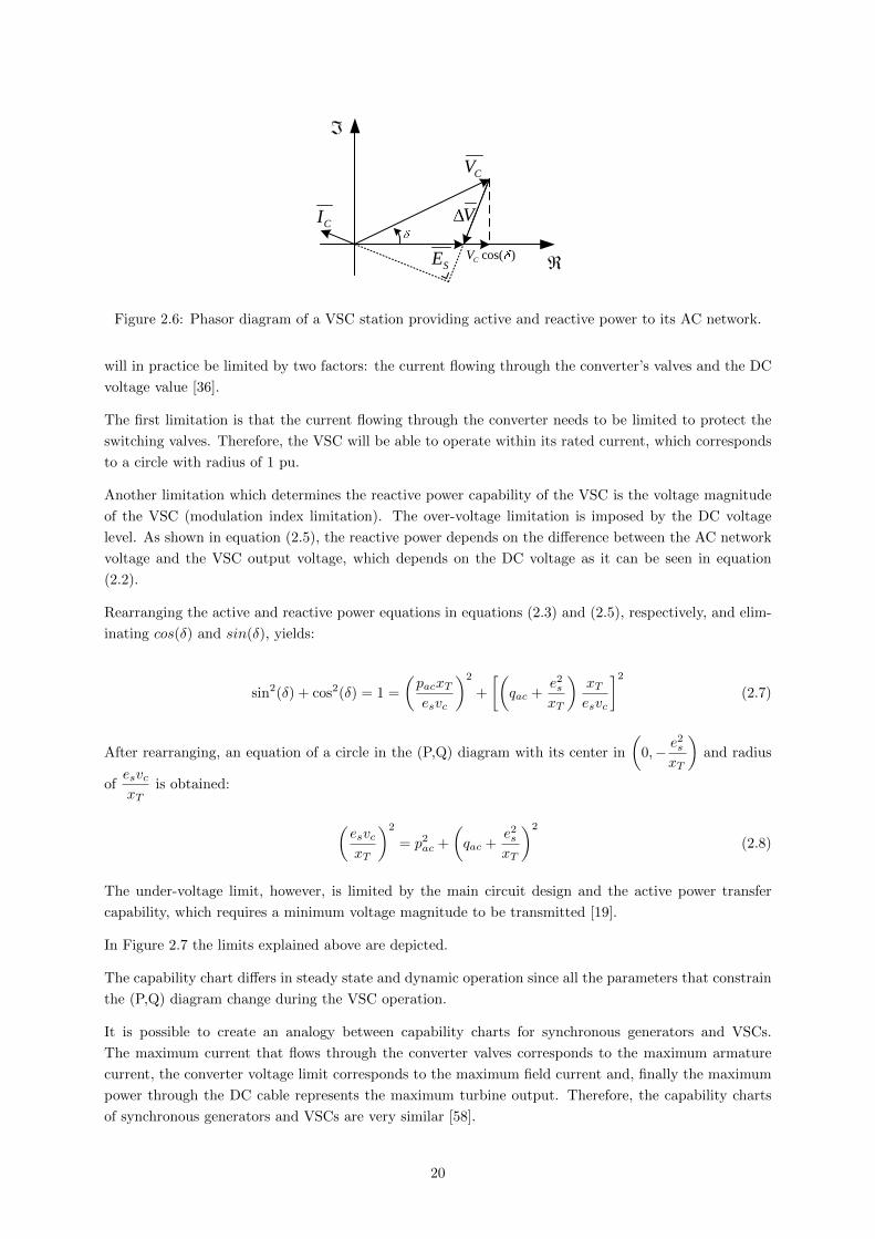
CI
CV
SE
V
cos( )CV
Figure 2.6: Phasor diagram of a VSC station providing active and reactive power to its AC network.
will in practice be limited by two factors: the current flowing through the converter’s valves and the DC
voltage value [36].
The first limitation is that the current flowing through the converter needs to be limited to protect the
switching valves. Therefore, the VSC will be able to operate within its rated current, which corresponds
to a circle with radius of 1 pu.
Another limitation which determines the reactive power capability of the VSC is the voltage magnitude
of the VSC (modulation index limitation). The over-voltage limitation is imposed by the DC voltage
level. As shown in equation (2.5), the reactive power depends on the difference between the AC network
voltage and the VSC output voltage, which depends on the DC voltage as it can be seen in equation
(2.2).
Rearranging the active and reactive power equations in equations (2.3) and (2.5), respectively, and elim-
inating cos(δ) and sin(δ), yields:
sin2(δ) + cos2(δ) = 1 =
(pacxTesvc
)2
+
[(qac +
e2sxT
)xTesvc
]2(2.7)
After rearranging, an equation of a circle in the (P,Q) diagram with its center in
(0,− e
2s
xT
)and radius
ofesvcxT
is obtained:
(esvcxT
)2
= p2ac +
(qac +
e2sxT
)2
(2.8)
The under-voltage limit, however, is limited by the main circuit design and the active power transfer
capability, which requires a minimum voltage magnitude to be transmitted [19].
In Figure 2.7 the limits explained above are depicted.
The capability chart differs in steady state and dynamic operation since all the parameters that constrain
the (P,Q) diagram change during the VSC operation.
It is possible to create an analogy between capability charts for synchronous generators and VSCs.
The maximum current that flows through the converter valves corresponds to the maximum armature
current, the converter voltage limit corresponds to the maximum field current and, finally the maximum
power through the DC cable represents the maximum turbine output. Therefore, the capability charts
of synchronous generators and VSCs are very similar [58].
20
acp
acq
2
s
T
e
x
s c
T
e v
x
| | 1.0Se pu
| | 1.1Se pu
| | 0.9Se pu
1st Limit
2nd Limit
1.0
0.5
-0.5
-1.0
1.0
-1.0
Figure 2.7: Real (P,Q) diagram of a VSC-HVDC station
21
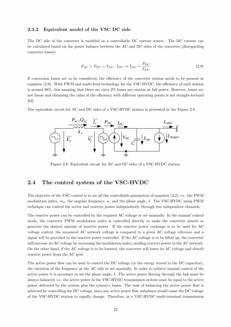
2.3.2 Equivalent model of the VSC DC side
The DC side of the converter is modeled as a controllable DC current source. The DC current can
be calculated based on the power balance between the AC and DC sides of the converter (disregarding
converter losses):
PAC = PDC = VDC · IDC ⇒ IDC =PDCVDC
(2.9)
If conversion losses are to be considered, the efficiency of the converter station needs to be present at
equation (2.9). With PWM and multi-level technology for the VSC-HVDC, the efficiency of each station
is around 98%, this meaning that there are circa 2% losses per station at full power. However, losses are
not linear and obtaining the value of the efficiency with different operating points is not straight-forward
[62].
The equivalent circuit for AC and DC sides of a VSC-HVDC station is presented in the Figure 2.8.
TX
CVSE
CI,AC ACP Q
IDC
VDC
PDC
C
Icable
IcapIchopper
Figure 2.8: Equivalent circuit for AC and DC sides of a VSC-HVDC station.
2.4 The control system of the VSC-HVDC
The objective of the VSC control is to set all the controllable parameters of equation (2.2), i.e. the PWM
modulation index, ma, the angular frequency, w, and the phase angle, δ. The VSC-HVDC using PWM
technique can control the active and reactive power independently through two independent channels.
The reactive power can be controlled by the required AC voltage or set manually. In the manual control
mode, the converter PWM modulation index is controlled directly to make the converter absorb or
generate the desired amount of reactive power. If the reactive power exchange is to be used for AC
voltage control, the measured AC network voltage is compared to a given AC voltage reference and a
signal will be provided to the reactive power controller. If the AC voltage is to be lifted up, the converter
will increase its AC voltage by increasing the modulation index, sending reactive power to the AC network.
On the other hand, if the AC voltage is to be lowered, the converter will lower its AC voltage and absorb
reactive power from the AC grid.
The active power flow can be used to control the DC voltage (or the energy stored in the DC capacitor),
the variation of the frequency at the AC side or set manually. In order to achieve manual control of the
active power it is necessary to set the phase angle, δ. The active power flowing through the link must be
always balanced, i.e. the active power in the VSC-HVDC transmission system must be equal to the active
power delivered by the system plus the system’s losses. The task of balancing the active power flow is
achieved by controlling the DC voltage, since any active power flow unbalance would cause the DC voltage
of the VSC-HVDC station to rapidly change. Therefore, in a VSC-HVDC multi-terminal transmission
22

system it is necessary that at least one station operates in DC voltage control mode, regulating the
amount of active power needed to charge or discharge the DC capacitor in order to sustain the required
DC voltage level. This way, the DC voltage controller will guarantee active power balance at all instants.
The frequency control is possible when the VSC is connected to weak networks or passive loads, i.e. the
VSC is the main source of power. The frequency control in such case is obtained by varying the frequency
of the valve pulse firing sequence.
Another important control in the VSC-HVDC is the AC current control. The VSC-HVDC control system
has an inner current control (ICC) that will receive the references of the currents from the outer controllers
and will generate the voltages’ references and provide them to the PWM control of the VSC. Figure 2.9
shows the control structure for the VSC-HVDC station.
Inner Current
Controller
AC Voltage
Controller
dqe
AC System
ACQ
*
ACQ
DCV
*
DCV
(*) reference
Active Power
Controller
Reactive Power
Controller
DC Voltage
Controller
Outer Controllers
C
*| |ACV
*
ACP
*
di
*
qi
*
dqu
Pac, Qac, |Vac|
calculator
PLL
abcv
abc to dq
dqiabc to dq
abci
ACP
| |ACV
dq to abc
*
abcu
DCVTX
PWM
Figure 2.9: VSC-HVDC Control Scheme.
2.4.1 Inner Current Controller
In the VSC-HVDC control system there is an inner current control that evaluates the necessary voltage
drop over the series reactance (XT ) to produce the required AC current without exceeding the converter
maximum current [51].
Usually in the inner current controller, the converter currents and the AC three-phase voltages are
transformed to the rotating direct-quadrature (dq) coordinate system, which will be synchronized with
the AC network voltage through a phase-locked loop (PLL). The control system will determinate the
converter voltage reference in the (dq) axis and this signal will be transformed to the three-phase (abc)
coordinate system before being provided to the converter’s PWM control.
23
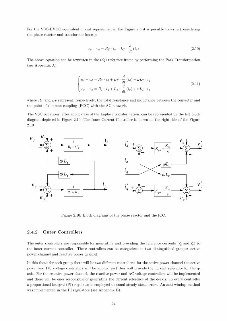
For the VSC-HVDC equivalent circuit represented in the Figure 2.5 it is possible to write (considering
the phase reactor and transformer losses):
es − vc = RT · ic + LT ·d
dt(ic) (2.10)
The above equation can be rewritten in the (dq) reference frame by performing the Park Transformation
(see Appendix A):
ed − vd = RT · id + LT ·
d
dt(id)− ωLT · iq
eq − vq = RT · iq + LT ·d
dt(iq) + ωLT · id
(2.11)
where RT and LT represent, respectively, the total resistance and inductance between the converter and
the point of common coupling (PCC) with the AC network.
The VSC equations, after application of the Laplace transformation, can be represented by the left block
diagram depicted in Figure 2.10. The Inner Current Controller is shown on the right side of the Figure
2.10.
TL
di
qi
qe
dedv
qv
TT sLR
1
TT sLR
1
TL
*
qi
*
di
di
qi
qe
de *
dv
*
qv
TL
s
KK
ii
ip
,
,
s
KK
ii
ip
,
,
TL
Figure 2.10: Block diagrams of the phase reactor and the ICC.
2.4.2 Outer Controllers
The outer controllers are responsible for generating and providing the reference currents (i∗d and i∗q) to
the inner current controller. These controllers can be categorized in two distinguished groups: active
power channel and reactive power channel.
In this thesis for each group there will be two different controllers: for the active power channel the active
power and DC voltage controllers will be applied and they will provide the current reference for the q-
axis. For the reactive power channel, the reactive power and AC voltage controllers will be implemented
and these will be ones responsible of generating the current reference of the d-axis. In every controller
a proportional-integral (PI) regulator is employed to annul steady state errors. An anti-windup method
was implemented in the PI regulators (see Appendix B).
24

Active and Reactive Power Outer Controllers
The active and reactive powers at the PCC in the (abc) frame can be calculated as [63]:
pac = vaia + vbib + vcic
qac =1√3
(vabic + vbcia + vcaib)(2.12)
If the Park-Transformation that conserves power from (abc) to (dq) frame is used and if the three-phase
system is balanced, the expressions above in the (dq) frame are given by:
pac = edid + eqiq
qac = eqid − ediq(2.13)
Moreover, it is assumed that the q-axis of the (dq) frame is aligned with the AC network voltage phasor
through a PLL, i.e. ed = 0, and the following expressions are obtained:
pac = eq · iqqac = eq · id
(2.14)
The above equations show that an independent control of the active and reactive power is possible
through the converter currents. The control diagrams are mathematically expressed in equation (2.15)
and in diagram form in Figure 2.11.
i∗d = (q∗ac − qac) ·
(Kp,q +
Ki,q
s
)i∗q = (p∗ac − pac) ·
(Kp,p +
Ki,p
s
) (2.15)
PAC
*
PAC
PAC
*
i q
*
s
KK
pi
pp
,
,
QAC
*
QAC
*
i d
*
QAC
s
KK
qi
qp
,
,
Figure 2.11: Active and reactive power outer controller diagrams.
DC Voltage Outer Controller
The objective of the DC voltage controller is to maintain the DC voltage at its reference value by
regulating the active power exchanged with the AC grid by regulating i∗q .
A DC voltage controller that operates on the error between the DC voltage and its reference value
(∆VDC = V ∗DC − VDC) could be applied, in an analogous way as in the active and reactive power outer
controllers. However, if the controller is to operate linearly on the DC voltage, the closed-loop dynamics
will be dependent on the operating point [61].
25
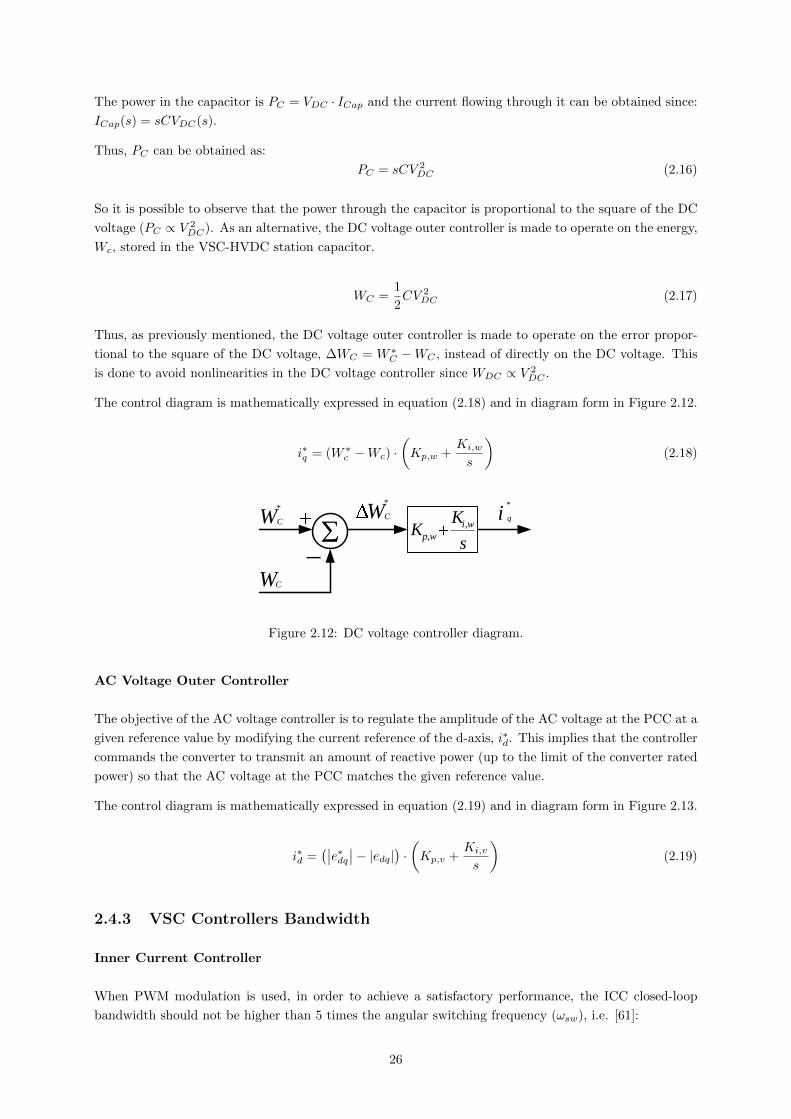
The power in the capacitor is PC = VDC · ICap and the current flowing through it can be obtained since:
ICap(s) = sCVDC(s).
Thus, PC can be obtained as:
PC = sCV 2DC (2.16)
So it is possible to observe that the power through the capacitor is proportional to the square of the DC
voltage (PC ∝ V 2DC). As an alternative, the DC voltage outer controller is made to operate on the energy,
Wc, stored in the VSC-HVDC station capacitor.
WC =1
2CV 2
DC (2.17)
Thus, as previously mentioned, the DC voltage outer controller is made to operate on the error propor-
tional to the square of the DC voltage, ∆WC = W ∗C −WC , instead of directly on the DC voltage. This
is done to avoid nonlinearities in the DC voltage controller since WDC ∝ V 2DC .
The control diagram is mathematically expressed in equation (2.18) and in diagram form in Figure 2.12.
i∗q = (W ∗c −Wc) ·
(Kp,w +
Ki,w
s
)(2.18)
WC
*
WC
WC
*
i q
*
s
KK wi
wp
,
,
Figure 2.12: DC voltage controller diagram.
AC Voltage Outer Controller
The objective of the AC voltage controller is to regulate the amplitude of the AC voltage at the PCC at a
given reference value by modifying the current reference of the d-axis, i∗d. This implies that the controller
commands the converter to transmit an amount of reactive power (up to the limit of the converter rated
power) so that the AC voltage at the PCC matches the given reference value.
The control diagram is mathematically expressed in equation (2.19) and in diagram form in Figure 2.13.
i∗d =(∣∣e∗dq∣∣− |edq|) · (Kp,v +
Ki,v
s
)(2.19)
2.4.3 VSC Controllers Bandwidth
Inner Current Controller
When PWM modulation is used, in order to achieve a satisfactory performance, the ICC closed-loop
bandwidth should not be higher than 5 times the angular switching frequency (ωsw), i.e. [61]:
26
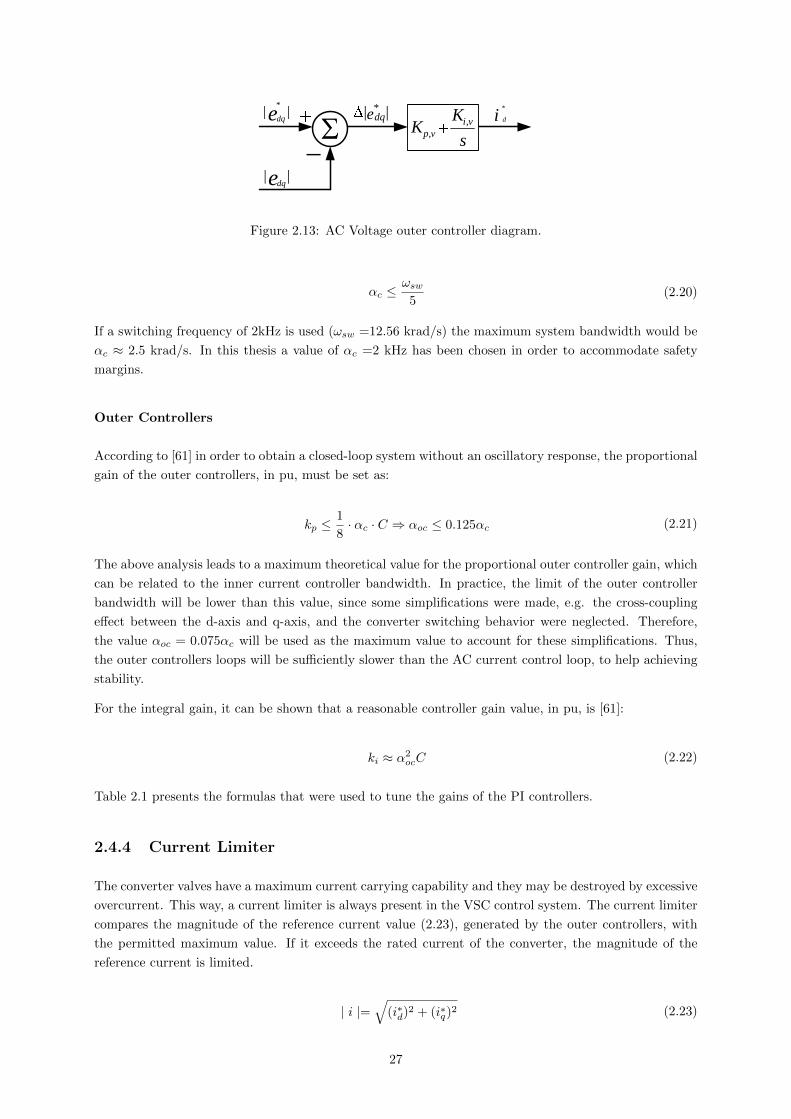
||*
edq|| *
edq i d
*
||edq
s
KK vi
vp
,
,
Figure 2.13: AC Voltage outer controller diagram.
αc ≤ωsw
5(2.20)
If a switching frequency of 2kHz is used (ωsw =12.56 krad/s) the maximum system bandwidth would be
αc ≈ 2.5 krad/s. In this thesis a value of αc =2 kHz has been chosen in order to accommodate safety
margins.
Outer Controllers
According to [61] in order to obtain a closed-loop system without an oscillatory response, the proportional
gain of the outer controllers, in pu, must be set as:
kp ≤1
8· αc · C ⇒ αoc ≤ 0.125αc (2.21)
The above analysis leads to a maximum theoretical value for the proportional outer controller gain, which
can be related to the inner current controller bandwidth. In practice, the limit of the outer controller
bandwidth will be lower than this value, since some simplifications were made, e.g. the cross-coupling
effect between the d-axis and q-axis, and the converter switching behavior were neglected. Therefore,
the value αoc = 0.075αc will be used as the maximum value to account for these simplifications. Thus,
the outer controllers loops will be sufficiently slower than the AC current control loop, to help achieving
stability.
For the integral gain, it can be shown that a reasonable controller gain value, in pu, is [61]:
ki ≈ α2ocC (2.22)
Table 2.1 presents the formulas that were used to tune the gains of the PI controllers.
2.4.4 Current Limiter
The converter valves have a maximum current carrying capability and they may be destroyed by excessive
overcurrent. This way, a current limiter is always present in the VSC control system. The current limiter
compares the magnitude of the reference current value (2.23), generated by the outer controllers, with
the permitted maximum value. If it exceeds the rated current of the converter, the magnitude of the
reference current is limited.
| i |=√
(i∗d)2 + (i∗q)
2 (2.23)
27

Table 2.1: Controllers’ gains.
Controller kp Kp ki Ki
ICC αcpu · Lp kp · ωb αcpu ·Rp ki · ωb
Active Power αocpu · Cpukp · IacbSb
α2ocpu · Cpu
ki · Iacb · ωbSb
Reactive Power αocpu · Cpukp · IacbSb
α2ocpu · Cpu
ki · Iacb · ωbSb
DC Voltage αocpu · Cpukp · IacbWb
α2ocpu · Cpu
ki · Iacb · ωbWb
AC Voltage αocpu · Cpukp · IacbVacb
α2ocpu · Cpu
ki · Iacb · ωbVacb
When | i | exceeds the maximum permitted value there are three different possible strategies to limit
the current (see Figure 2.14). Priority can be given to voltage restoration (reactive power priority) and
therefore, the d-axis current will be maintained and q-axis will be reduced. This strategy is normally
chosen if the converter is connected to a weak grid or used to supply an industrial plant.
If the converter is connected to a strong grid the priority is usually given to the delivery of active power
(q-axis current will stay unchanged and the d-axis current will be reduced). The last method is to
proportionally limit the current in both axis, maintaining then the power factor constant.
q
d
*
qi**
qi
***
dd ii
q
d
*
qi**
qi
*
di**
di
d-axis priority Proportional current limiter
q
d*
di**
di
***
qq ii
q-axis priority
Figure 2.14: Current limiting strategies.
28

Chapter 3
Multi-Terminal DC Networks
3.1 Introduction
There are more than 100 HVDC transmission systems installed all over the world, but only three have
more than two terminals: the Hydro-Quebec/New England system, in Canada [5]; the SACOI-2, con-
necting Italy and France [21], and a back-to-back scheme using VSC technology at the Shin-Shinano
substation, in Japan [45]. All the aforementioned systems have 3 terminals.
In order to create a multi-terminal grid, the stations can be either connected in series or in parallel.
When connected in series all the stations share the same current. On the other hand, for the parallel
connection the stations share the same DC transmission voltage [21]. There are several possibilities for
the grid’s topology: shore-to-shore, radial, meshed, cluster with multi-way interconnector, a combination
of interconnectors and meshed grids, etc.. In Figure 3.1 it is shown the network topologies that are
possible according to the HVDC technology implemented.
MTDC
VSC CSC Hybrid
Parallel Series
Radial Meshed
Network
Topology
HVDC
technology
Figure 3.1: MTDC Network classification scheme.
The VSC technology created the possibility of building true MTDC grids which has been difficult with
the use of CSC technology. Some of the main reasons for this are: the limitations of thyristor based
HVDC to 2-quadrant operation while used in multiterminal topology, the need for supply of reactive
power at each terminal, and the difficult control structure (see Chapter 1).
29
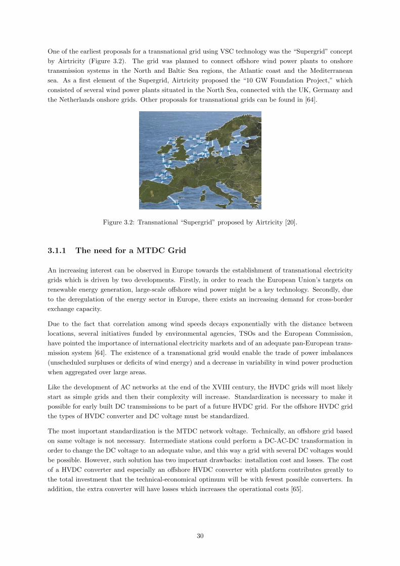
One of the earliest proposals for a transnational grid using VSC technology was the “Supergrid” concept
by Airtricity (Figure 3.2). The grid was planned to connect offshore wind power plants to onshore
transmission systems in the North and Baltic Sea regions, the Atlantic coast and the Mediterranean
sea. As a first element of the Supergrid, Airtricity proposed the “10 GW Foundation Project,” which
consisted of several wind power plants situated in the North Sea, connected with the UK, Germany and
the Netherlands onshore grids. Other proposals for transnational grids can be found in [64].
Figure 3.2: Transnational “Supergrid” proposed by Airtricity [20].
3.1.1 The need for a MTDC Grid
An increasing interest can be observed in Europe towards the establishment of transnational electricity
grids which is driven by two developments. Firstly, in order to reach the European Union’s targets on
renewable energy generation, large-scale offshore wind power might be a key technology. Secondly, due
to the deregulation of the energy sector in Europe, there exists an increasing demand for cross-border
exchange capacity.
Due to the fact that correlation among wind speeds decays exponentially with the distance between
locations, several initiatives funded by environmental agencies, TSOs and the European Commission,
have pointed the importance of international electricity markets and of an adequate pan-European trans-
mission system [64]. The existence of a transnational grid would enable the trade of power imbalances
(unscheduled surpluses or deficits of wind energy) and a decrease in variability in wind power production
when aggregated over large areas.
Like the development of AC networks at the end of the XVIII century, the HVDC grids will most likely
start as simple grids and then their complexity will increase. Standardization is necessary to make it
possible for early built DC transmissions to be part of a future HVDC grid. For the offshore HVDC grid
the types of HVDC converter and DC voltage must be standardized.
The most important standardization is the MTDC network voltage. Technically, an offshore grid based
on same voltage is not necessary. Intermediate stations could perform a DC-AC-DC transformation in
order to change the DC voltage to an adequate value, and this way a grid with several DC voltages would
be possible. However, such solution has two important drawbacks: installation cost and losses. The cost
of a HVDC converter and especially an offshore HVDC converter with platform contributes greatly to
the total investment that the technical-economical optimum will be with fewest possible converters. In
addition, the extra converter will have losses which increases the operational costs [65].
30
Reliability and Redundancy
All the offshore wind power plants built until now use a single cable as a connection to the shore. Thus,
this type of connection has no redundancy. The reliability of the connection critically relies on some of
its main components, most importantly the cable circuit connecting the wind power plant to the onshore
grid. When malfunctioning, these components will take the complete installation out of service.
With the expected increase of the offshore wind power capacity in the future, this situation will probably
change. TSOs may start putting requirements on the availability of the connection and then the loss of
production due to an offshore transmission outage will become a manageable risk.
Transnational offshore grids are expected to improve reliability. They will have several connection points
to the onshore grids and in that way there will be always an alternative path along which the power, or
part of it, can be evacuated.
Flexibility, Standardization, and Modularity
The development of offshore wind power and offshore transmission system will probably take over a
decade. Thus, it is difficult, in the present, to determinate a detailed blueprint of such infrastructure.
The evolution of offshore infrastructure is a gradual process that constantly needs to adapt to new
developments in the industry and society as a whole. However, since the nodes in this offshore network,
i.e. substations located on offshore platforms, will be difficult to modify or extend once installed, it is
crucial for the success of such network to consider future expansion plans right from the beginning. For
optimal results, such offshore grid expansion plans should be the result of coordinated efforts among the
responsible authorities.
Controllability of Power Flows
Due to the fact that an offshore transnational grid will likely be based on HVDC technology, it will
have higher controllability of power flows than onshore AC grids, where the distribution of power flows
results from the dispatch of generators and the impedance of the transmission lines. However, the power
flow can be influenced indirectly e.g. via additional equipment such as phase-shifting transformers.
HVDC technology inherently enables forcing a predefined power flow along a certain transmission cable.
This feature will have an impact on the rules for congestion management for such grid. Nowadays,
there are different rules among the European electrical markets for the priority dispatch of renewable
energy sources, including onshore and offshore wind. Some markets, such as the German one, always give
precedence to generation from renewable sources, whereas others, e.g. the Dutch market, renewables have
an equal status as any other generation source. The creation of a transnational offshore grid would create
a coupling of these markets and, hence, it will be necessary a harmonization of market and operation
rules.
3.1.2 Applications of a MTDC grid
Beyond the time horizon of 2020, offshore wind power plants are expected to have higher power ratings
and to be situated further from the shore. This implies that the costs of the electrical infrastructure will
constitute a higher share in the total investment costs. Therefore, methods to increase the utilization of
the connection are attractive.
31

An increased need for interconnection capacity between European countries is leaded by market coupling
and balancing of the variable output of renewables. Offshore wind power plant connections can be com-
bined with interconnectors between countries to increase the utilization of the electrical infrastructure
and, hence, to reduce costs. Cost-effective networks demand an overall optimized grid design that avoids
suboptimal solutions based on individual and national projects. To achieve an optimal solution cooper-
ation among countries is also recommended: harmonization of legal rules, simplification of authorization
procedures and international spatial maritime planning.
An interconnection between offshore wind farms, oil and gas platforms and onshore grids can result in
reduced operational costs, increased reliability and reduced CO2 emissions. In most offshore installations,
power supply generators and large compressors are driven by onboard gas turbines or diesel engines. Many
of these power sources have efficiencies around 20-25% under the best assumptions. The result is the
emission of large amounts of CO2 emission and unnecessary high fuel consumption. If the electrical power
can be supplied from the DC grid, CO2 emissions from offshore installations are eliminated. This leads
to a significant cost savings for oil companies. In addition, transmission of electrical energy from the DC
grid involves less maintenance, longer lifetime and higher availability than gas turbines and diesel engines.
If the transmission equipment can be located on decommissioned offshore installations, the postponed
removal cost for the installation can be an important factor as well [66].
The offshore potential in Europe consists both of wind energy and ocean energy. The term ocean energy
includes wave energy, tidal current, tidal range, osmotic energy and ocean thermal energy. West European
coasts have high wave energy potential (see Figure 3.3). Nonetheless, in areas with low wave energy
potential such as the North Sea, wave energy converters can produce 10-75 TWh/y [27].
Figure 3.3: Wave energy in Europe in kW/m width of oncoming wave.
The wave and tidal energy converters are located on the sea surface or below it, whereas offshore wind
turbines use their respective resource tens of meters above the sea level. Therefore, wave and tidal energy
converters can be deployed between offshore wind turbines since there has to be a certain distance among
the turbines to avoid shadow effects. Placed together, they can share the same offshore grid. Therefore,
installation costs would be reduced since the cable costing is not a linear function of the number of the
cables as the same route and laying procedure might be applied for more than one cable.
A combination of the power output of both resources would result in smoother variations of the generated
power, better predictability and higher capacity credit, since wave energy peaks generally occurs 6-8 h
later than wind energy peaks, and because wave energy has greater predictability and less variability
when compared to wind energy [27].
Differently from an AC system, with a DC grid it is possible to collect power from multiple non-
32
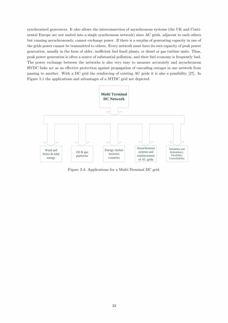
synchronized generators. It also allows the interconnection of asynchronous systems (the UK and Conti-
nental Europe are not united into a single synchronous network) since AC grids, adjacent to each others
but running asynchronously, cannot exchange power. If there is a surplus of generating capacity in one of
the grids power cannot be transmitted to others. Every network must have its own capacity of peak power
generation, usually in the form of older, inefficient fuel fossil plants, or diesel or gas turbine units. Thus,
peak power generation is often a source of substantial pollution, and their fuel economy is frequently bad.
The power exchange between the networks is also very easy to measure accurately and asynchronous
HVDC links act as an effective protection against propagation of cascading outages in one network from
passing to another. With a DC grid the reinforcing of existing AC grids it is also a possibility [27]. In
Figure 5.1 the applications and advantages of a MTDC grid are depicted.
Wind and
Wave & tidal
energy
Multi Terminal
DC Network
Oil & gas
platforms
Energy market
between
countries
Asynchronous
systems and
reinforcement
of AC grids
Reliability and
Redundancy,
Flexibility,
Controllability
Figure 3.4: Applications for a Multi-Terminal DC grid.
33

3.2 State-space model of MTDC grids
3.2.1 Meshed MTDC grid
In this section a state-space model for a grid composed of 3 VSC stations will be derived. The grid
considered is shown in Figure 3.5. Each station is connected through a DC cable to the others nodes in
the network, thus forming a meshed grid.
1DCV1LI
2L
I
11C12C
31C
32C
21C
22C
3Z
1Z
2Z
1DCI2DCI
3DCI
2DCV
3DCV
3LI
Figure 3.5: Example of a meshed-connected VSC-HVDC MTDC network with three terminals.
The incidence matrix, IM , which contains the information about the existing DC cables in the grid
considered, is given by:
IM =
1 −1 0
1 0 −1
0 1 −1
L×N
(3.1)
where the value 1 means that the current is flowing from the node, and -1 means that the current is
flowing to the node. The letter N stands for the number of nodes and L for the number of cables of the
MTDC grid.
The application of Kirchhoff’s current law (KCL) on each node, yields:
• IDC1 = IC11 + IC21 + IL1 + IL2 ⇔
IDC1 = sC11VDC1 + sC21VDC1 + IL1 + IL2 ⇔
sVDC1 =IDC1 − IL1 − IL2
C11 + C21
(3.2)
• IDC2 = IC12 + IC31 − IL1 + IL3 ⇔
IDC2 = sC12VDC2 + sC31VDC2 − IL1 + IL3 ⇔
sVDC2 =IDC2 + IL1 − IL3
C12 + C31
(3.3)
• IDC3 = IC22 + IC32 − IL2 − IL3 ⇔
IDC3 = sC22VDC3 + sC32VDC3 − IL2 − IL3 ⇔
sVDC3 =IDC3 + IL2 + IL3
C22 + C32
(3.4)
34
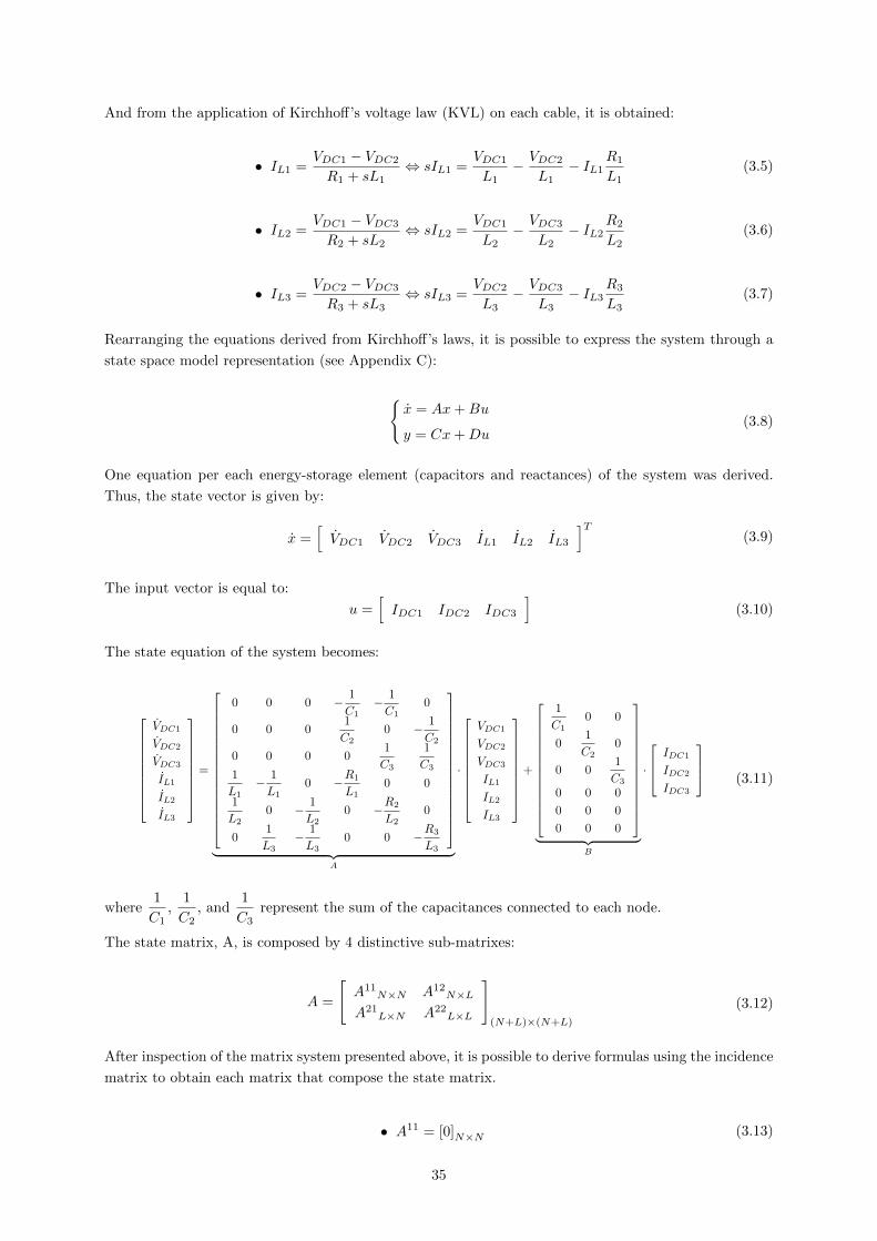
And from the application of Kirchhoff’s voltage law (KVL) on each cable, it is obtained:
• IL1 =VDC1 − VDC2
R1 + sL1⇔ sIL1 =
VDC1
L1− VDC2
L1− IL1
R1
L1(3.5)
• IL2 =VDC1 − VDC3
R2 + sL2⇔ sIL2 =
VDC1
L2− VDC3
L2− IL2
R2
L2(3.6)
• IL3 =VDC2 − VDC3
R3 + sL3⇔ sIL3 =
VDC2
L3− VDC3
L3− IL3
R3
L3(3.7)
Rearranging the equations derived from Kirchhoff’s laws, it is possible to express the system through a
state space model representation (see Appendix C):
x = Ax+Bu
y = Cx+Du(3.8)
One equation per each energy-storage element (capacitors and reactances) of the system was derived.
Thus, the state vector is given by:
x =[VDC1 VDC2 VDC3 IL1 IL2 IL3
]T(3.9)
The input vector is equal to:
u =[IDC1 IDC2 IDC3
](3.10)
The state equation of the system becomes:
VDC1
VDC2
VDC3
IL1
IL2
IL3
=
0 0 0 − 1
C1− 1
C10
0 0 01
C20 − 1
C2
0 0 0 01
C3
1
C31
L1− 1
L10 −R1
L10 0
1
L20 − 1
L20 −R2
L20
01
L3− 1
L30 0 −R3
L3
︸ ︷︷ ︸
A
·
VDC1
VDC2
VDC3
IL1
IL2
IL3
+
1
C10 0
01
C20
0 01
C3
0 0 0
0 0 0
0 0 0
︸ ︷︷ ︸
B
·
IDC1
IDC2
IDC3
(3.11)
where1
C1,
1
C2, and
1
C3represent the sum of the capacitances connected to each node.
The state matrix, A, is composed by 4 distinctive sub-matrixes:
A =
[A11
N×N A12N×L
A21L×N A22
L×L
](N+L)×(N+L)
(3.12)
After inspection of the matrix system presented above, it is possible to derive formulas using the incidence
matrix to obtain each matrix that compose the state matrix.
• A11 = [0]N×N (3.13)
35

• −A12T =
1 −1 0
1 0 −1
0 1 −1
L×N
×
1
C10 0
01
C20
0 01
C3
N×N
=
1
C1− 1
C20
1
C10 − 1
C3
01
C2− 1
C3
L×N
⇒ A12 =
− 1
C1− 1
C10
1
C20 − 1
C2
01
C3
1
C3
N×L
(3.14)
• A21 =
1
L10 0
01
L20
0 01
L3
L×L
×
1 −1 0
1 0 −1
0 1 −1
L×N
=
1
L1− 1
L10
1
L20 − 1
L2
01
L3− 1
L3
L×N
(3.15)
• A22 =
−R1
L10 0
0 −R2
L20
0 0 −R3
L3
L×L
(3.16)
The input matrix, B, is also composed by 2 different sub-matrixes.
B =
[B11
N×N
B21L×N
](N+L)×N
(3.17)
• B11 =
1
C10 0
01
C20
0 01
C3
N×N
(3.18)
• B21 = [0]L×N (3.19)
It is possible to observe that all the matrixes derived above are dependent of the grid configuration, but
the necessary information is obtained from the incidence matrix, IM .
The output equation is given by:
VDC1
VDC2
VDC3
IL1
IL2
IL3
= I︸︷︷︸
C
·
VDC1
VDC2
VDC3
IL1
IL2
IL3
+ 0︸︷︷︸
D
·
IDC1
IDC2
IDC3
(3.20)
36

The output matrix, C, is an identity matrix since there is no need for combinations of state variables in
the output.
C = [I](N+L)×(N+L) (3.21)
Given the fact that there are no current sources present in the grid, the direct transition matrix, D, is
only filled with zeros.
D = [0](N+L)×N (3.22)
3.2.2 Radial MTDC grid
In this section a state-space model for a grid composed by 4 stations will be derived. The grid considered
is shown in Figure 3.6. Each station is connected to a central point, forming this way a radial grid.
1DCV
2DCV
3DCV
4DCV
5DCV
1LI
2LI
3LI
4LI
11C12C
21C22C 42C 41C
31C32C
4Z2Z
1Z 3Z1DCI
2DCI 4DCI
3DCI
5DCI
Figure 3.6: Example of a radially-connected VSC-HVDC MTDC network with four terminals.
The incidence matrix, IM , for this grid is given by:
IM =
1 0 0 0 −1
0 1 0 0 −1
0 0 1 0 −1
0 0 0 1 −1
L×N
(3.23)
Once again the Kirchhoff’s laws are applied. The application of KCL on each node, yields:
• IDC1 = IC11 + IL1 ⇔ IDC1 = sC11VDC1 + IL1 ⇔ sVDC1 =IDC1 − IL1
C11(3.24)
• IDC2 = IC21 + IL2 ⇔ IDC2 = sC21VDC2 + IL2 ⇔ sVDC2 =IDC2 − IL2
C21(3.25)
• IDC3 = IC31 + IL3 ⇔ IDC3 = sC31VDC3 + IL3 ⇔ sVDC3 =IDC3 − IL3
C31(3.26)
• IDC4 = IC41 + IL4 ⇔ IDC4 = sC41VDC4 + I41 ⇔ sVDC4 =IDC4 − IL4
C41(3.27)
37
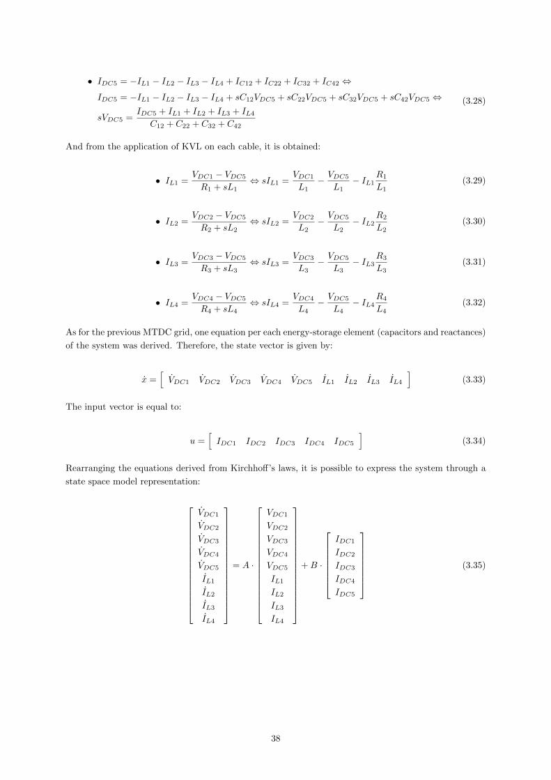
• IDC5 = −IL1 − IL2 − IL3 − IL4 + IC12 + IC22 + IC32 + IC42 ⇔
IDC5 = −IL1 − IL2 − IL3 − IL4 + sC12VDC5 + sC22VDC5 + sC32VDC5 + sC42VDC5 ⇔
sVDC5 =IDC5 + IL1 + IL2 + IL3 + IL4
C12 + C22 + C32 + C42
(3.28)
And from the application of KVL on each cable, it is obtained:
• IL1 =VDC1 − VDC5
R1 + sL1⇔ sIL1 =
VDC1
L1− VDC5
L1− IL1
R1
L1(3.29)
• IL2 =VDC2 − VDC5
R2 + sL2⇔ sIL2 =
VDC2
L2− VDC5
L2− IL2
R2
L2(3.30)
• IL3 =VDC3 − VDC5
R3 + sL3⇔ sIL3 =
VDC3
L3− VDC5
L3− IL3
R3
L3(3.31)
• IL4 =VDC4 − VDC5
R4 + sL4⇔ sIL4 =
VDC4
L4− VDC5
L4− IL4
R4
L4(3.32)
As for the previous MTDC grid, one equation per each energy-storage element (capacitors and reactances)
of the system was derived. Therefore, the state vector is given by:
x =[VDC1 VDC2 VDC3 VDC4 VDC5 IL1 IL2 IL3 IL4
](3.33)
The input vector is equal to:
u =[IDC1 IDC2 IDC3 IDC4 IDC5
](3.34)
Rearranging the equations derived from Kirchhoff’s laws, it is possible to express the system through a
state space model representation:
VDC1
VDC2
VDC3
VDC4
VDC5
IL1
IL2
IL3
IL4
= A ·
VDC1
VDC2
VDC3
VDC4
VDC5
IL1
IL2
IL3
IL4
+B ·
IDC1
IDC2
IDC3
IDC4
IDC5
(3.35)
38

where A is given by:
A =
0 0 0 0 0 − 1
C10 0 0
0 0 0 0 0 0 − 1
C20 0
0 0 0 0 0 0 0 − 1
C30
0 0 0 0 0 0 0 0 − 1
C4
0 0 0 0 01
C5
1
C5
1
C5
1
C51
L10 0 0 − 1
L1−R1
L10 0 0
01
L20 0 − 1
L20 −R2
L20 0
0 01
L30 − 1
L30 0 −R3
L30
0 0 01
L4− 1
L40 0 0 −R4
L4
(N+L)×(N+L)
(3.36)
and B by:
B =
1
C10 0 0 0
01
C20 0 0
0 01
C30 0
0 0 01
C40
0 0 0 01
C5
0 0 0 0 0
0 0 0 0 0
0 0 0 0 0
0 0 0 0 0
(N+L)×N
(3.37)
Once again the state matrix, A, is composed by 4 distinctive sub-matrixes:
A =
[A11
N×N A12N×L
A21L×N A22
L×L
](N+L)×(N+L)
(3.38)
Using the same approach as before the formulas to obtain the sub-matrixes that constitute the state
matrix were derived:
• A11 = [0]N×N (3.39)
39
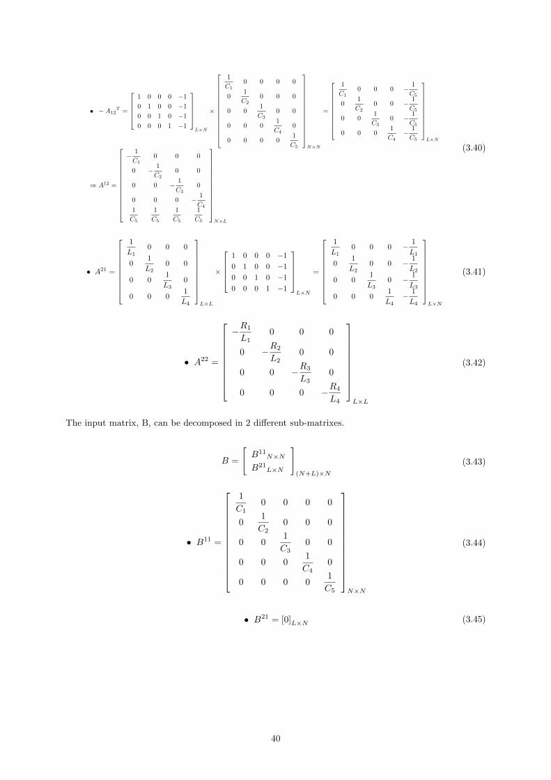
• −A12T =
1 0 0 0 −1
0 1 0 0 −1
0 0 1 0 −1
0 0 0 1 −1
L×N
×
1
C10 0 0 0
01
C20 0 0
0 01
C30 0
0 0 01
C40
0 0 0 01
C5
N×N
=
1
C10 0 0 − 1
C5
01
C20 0 − 1
C5
0 01
C30 − 1
C5
0 0 01
C4− 1
C5
L×N
⇒ A12 =
− 1
C10 0 0
0 − 1
C20 0
0 0 − 1
C30
0 0 0 − 1
C41
C5
1
C5
1
C5
1
C5
N×L
(3.40)
• A21 =
1
L10 0 0
01
L20 0
0 01
L30
0 0 01
L4
L×L
×
1 0 0 0 −1
0 1 0 0 −1
0 0 1 0 −1
0 0 0 1 −1
L×N
=
1
L10 0 0 − 1
L1
01
L20 0 − 1
L2
0 01
L30 − 1
L3
0 0 01
L4− 1
L4
L×N
(3.41)
• A22 =
−R1
L10 0 0
0 −R2
L20 0
0 0 −R3
L30
0 0 0 −R4
L4
L×L
(3.42)
The input matrix, B, can be decomposed in 2 different sub-matrixes.
B =
[B11
N×N
B21L×N
](N+L)×N
(3.43)
• B11 =
1
C10 0 0 0
01
C20 0 0
0 01
C30 0
0 0 01
C40
0 0 0 01
C5
N×N
(3.44)
• B21 = [0]L×N (3.45)
40
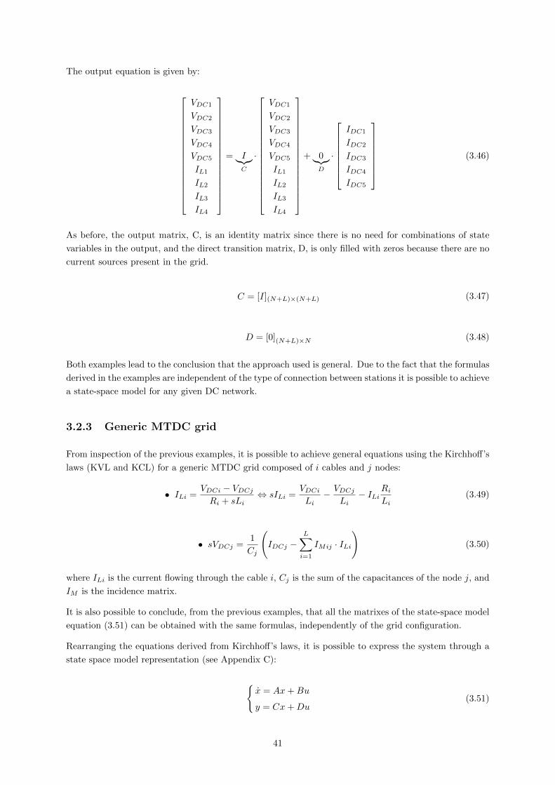
The output equation is given by:
VDC1
VDC2
VDC3
VDC4
VDC5
IL1
IL2
IL3
IL4
= I︸︷︷︸
C
·
VDC1
VDC2
VDC3
VDC4
VDC5
IL1
IL2
IL3
IL4
+ 0︸︷︷︸
D
·
IDC1
IDC2
IDC3
IDC4
IDC5
(3.46)
As before, the output matrix, C, is an identity matrix since there is no need for combinations of state
variables in the output, and the direct transition matrix, D, is only filled with zeros because there are no
current sources present in the grid.
C = [I](N+L)×(N+L) (3.47)
D = [0](N+L)×N (3.48)
Both examples lead to the conclusion that the approach used is general. Due to the fact that the formulas
derived in the examples are independent of the type of connection between stations it is possible to achieve
a state-space model for any given DC network.
3.2.3 Generic MTDC grid
From inspection of the previous examples, it is possible to achieve general equations using the Kirchhoff’s
laws (KVL and KCL) for a generic MTDC grid composed of i cables and j nodes:
• ILi =VDCi − VDCjRi + sLi
⇔ sILi =VDCiLi− VDCj
Li− ILi
RiLi
(3.49)
• sVDCj =1
Cj
(IDCj −
L∑i=1
IMij · ILi
)(3.50)
where ILi is the current flowing through the cable i, Cj is the sum of the capacitances of the node j, and
IM is the incidence matrix.
It is also possible to conclude, from the previous examples, that all the matrixes of the state-space model
equation (3.51) can be obtained with the same formulas, independently of the grid configuration.
Rearranging the equations derived from Kirchhoff’s laws, it is possible to express the system through a
state space model representation (see Appendix C):
x = Ax+Bu
y = Cx+Du(3.51)
41

One equation per each energy-storage element (capacitors and reactances) of the system has to be derived.
Therefore, the state vector will be given by:
x =[VDC1 VDC2 · · · VDCj IL1 IL2 · · · ILi
]1×(N+L)
(3.52)
The input vector is equal to:
u =[IDC1 IDC2 · · · IDCj
]1×N
(3.53)
The state equation of the system becomes:
VDC1
VDC2
...
VDCj
IL1
IL2...
ILi
= A ·
VDC1
VDC2
...
VDCj
IL1
IL2...
ILi
+B ·
IDC1
IDC2
...
IDCj
(3.54)
The state matrix, A, is composed of 4 sub-matrixes:
A =
[A11
N×N A12N×L
A21L×N A22
L×L
](N+L)×(N+L)
(3.55)
Which can be obtained by:
• A11 = [0]N×N (3.56)
• A12 = −
IM ·
1
C10 · · · 0
01
C2
. . ....
.... . .
. . . 0
0 · · · 01
Cj
T
N×L
(3.57)
A21 =
1
L10 · · · 0
01
L2
. . ....
.... . .
. . . 0
0 · · · 01
Li
· IM
L×N
(3.58)
42

• A22 =
−R1
L10 · · · 0
0 −R2
L2
. . ....
.... . .
. . . 0
0 · · · 0 −RiLi
L×L
(3.59)
The input matrix, B, which is constituted by 2 sub-matrixes, can be calculated as:
B =
[B11
N×N
B21L×N
](N+L)×N
(3.60)
• B11 =
1
C10 · · · 0
01
C2
. . ....
.... . .
. . . 0
0 · · · 01
Cj
N×N
(3.61)
• B21 = [0]L×N (3.62)
Finally, the output matrix, C, and the direct transition matrix, D, from the output equation are given
by:
C = [I](N+L)×(N+L) (3.63)
D = [0](N+L)×N (3.64)
With the method derived it is possible to obtain a state-space model for a general DC grid. Due to the
fact that the matrixes are derived from the information contained in the incidence matrix, this approach
allows to easily change the grid topology.
43
Chapter 4
DC Voltage Control Methods
4.1 Introduction
When a MTDC system is concerned, the DC voltage control is indubitably one of the most important
tasks of the VSC-HVDC transmission system. The DC voltage must be well controlled within stiff
limits under all conditions in order to guarantee power balance between all transmission terminals inside
the MTDC network. If the DC voltage increases excessively, it may trigger protection equipment (e.g.
DC choppers plus resistors). Low DC voltage values can give rise to non-linear phenomena of PWM
modulation and negatively affecting the linear stability of the control systems. Furthermore, a relatively
large DC voltage drop might, temporarily, limit the capability of the AC voltage controller [67].
In most cases, in a point-to-point HVDC transmission system, one of the terminals controls the DC voltage
of the transmission link while the other terminal controls the active power sent to the interconnection.
However, when a MTDC network is considered, it may be very difficult to operate the system with just
one converter station controlling the DC voltage, as in the previous case. This is due to mainly two
reasons: limited power rating of the VSC station controlling the DC voltage and the possibility of faults
in the AC network connected to that station which could trigger protection equipment within only a few
cycles of the AC network. Therefore, giving the DC voltage control to more than one VSC station seems
to be a better option to operate a MTDC system.
In future transnational offshore networks, several offshore wind farms and countries will be interconnected
and different market dispatch schemes may be applied among the onshore stations to share the power
from the wind farms as well as to perform power trade among them. There are three dispatch possibilities
that may be applied: fixed power sharing, priority power sharing and proportional power sharing.
In order to have such dispatch possibilities, control strategies capable of performing different market
dispatch schemes in the future transnational network are required. Besides the capability of performing
different market dispatch schemes during normal operation, the control strategies have to be capable of
acceptably performing during and after disturbances, e.g. voltage dip at an onshore grid or disconnection
of an onshore station. Moreover, it is also required that the control scheme must be independent of the
network topology to avoid unsuitable operation points upon changes in the network, e.g. expansion of the
DC grid and subsequently addition of new transmission cables or temporary disconnection of an existing
cable for maintenance purposes. Furthermore, if the control system requires communication, in order to
perform the dispatch schemes, with an outer remote controller, such as a transmission system operator
(TSO), it is important that the control strategy should be capable of performing acceptable operation
during communication delays or failure.
44

4.2 Market dispatch schemes
In this section the market dispatch schemes are explained in detail. These schemes will be, most certainly,
implemented in a future offshore transnational MTDC grid.
Fixed power sharing
When in fixed power sharing, one onshore station receives a fixed amount of active power and the other
stations will balance the power generation variability of the offshore wind farms. The active power
transmitted to the priority station may be generated at the offshore wind farms, come from the others
onshore stations, or part of the power may be generated at the offshore wind farms and the rest of the
power will be transmitted from the others onshore stations.
Priority power sharing
In priority power sharing, one station has priority in terms of transmitting the power generated by the
offshore wind farms over the others onshore stations. Thus, it obtains all the offshore generated power
up to a particular limit set by the system operators while the other stations receive the excess power to
balance the DC voltage inside the grid.
Therefore, while the power delivered to the priority station does not reach the limit, the other onshore
stations will not receive power from the wind farms.
Proportional power sharing
If a proportional power sharing scheme is implemented, the onshore stations share the power in a propor-
tion set by the system operator. The supervisory controller measures the offshore power being generated
and then calculates the amount of power that each station will receive according to the ratio defined,
which may be changed from time to time.
45
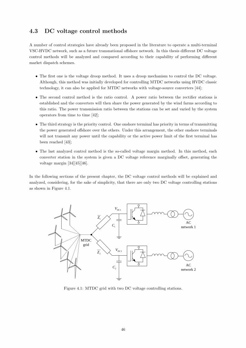
4.3 DC voltage control methods
A number of control strategies have already been proposed in the literature to operate a multi-terminal
VSC-HVDC network, such as a future transnational offshore network. In this thesis different DC voltage
control methods will be analyzed and compared according to their capability of performing different
market dispatch schemes.
• The first one is the voltage droop method. It uses a droop mechanism to control the DC voltage.
Although, this method was initially developed for controlling MTDC networks using HVDC classic
technology, it can also be applied for MTDC networks with voltage-source converters [44];
• The second control method is the ratio control. A power ratio between the rectifier stations is
established and the converters will then share the power generated by the wind farms according to
this ratio. The power transmission ratio between the stations can be set and varied by the system
operators from time to time [42];
• The third strategy is the priority control. One onshore terminal has priority in terms of transmitting
the power generated offshore over the others. Under this arrangement, the other onshore terminals
will not transmit any power until the capability or the active power limit of the first terminal has
been reached [43];
• The last analyzed control method is the so-called voltage margin method. In this method, each
converter station in the system is given a DC voltage reference marginally offset, generating the
voltage margin [34][45][46].
In the following sections of the present chapter, the DC voltage control methods will be explained and
analyzed, considering, for the sake of simplicity, that there are only two DC voltage controlling stations
as shown in Figure 4.1.
AC
network 1
AC
network 2
1Z
2Z
2C
1C
1DCV
2DCV
MTDC
grid
Figure 4.1: MTDC grid with two DC voltage controlling stations.
46
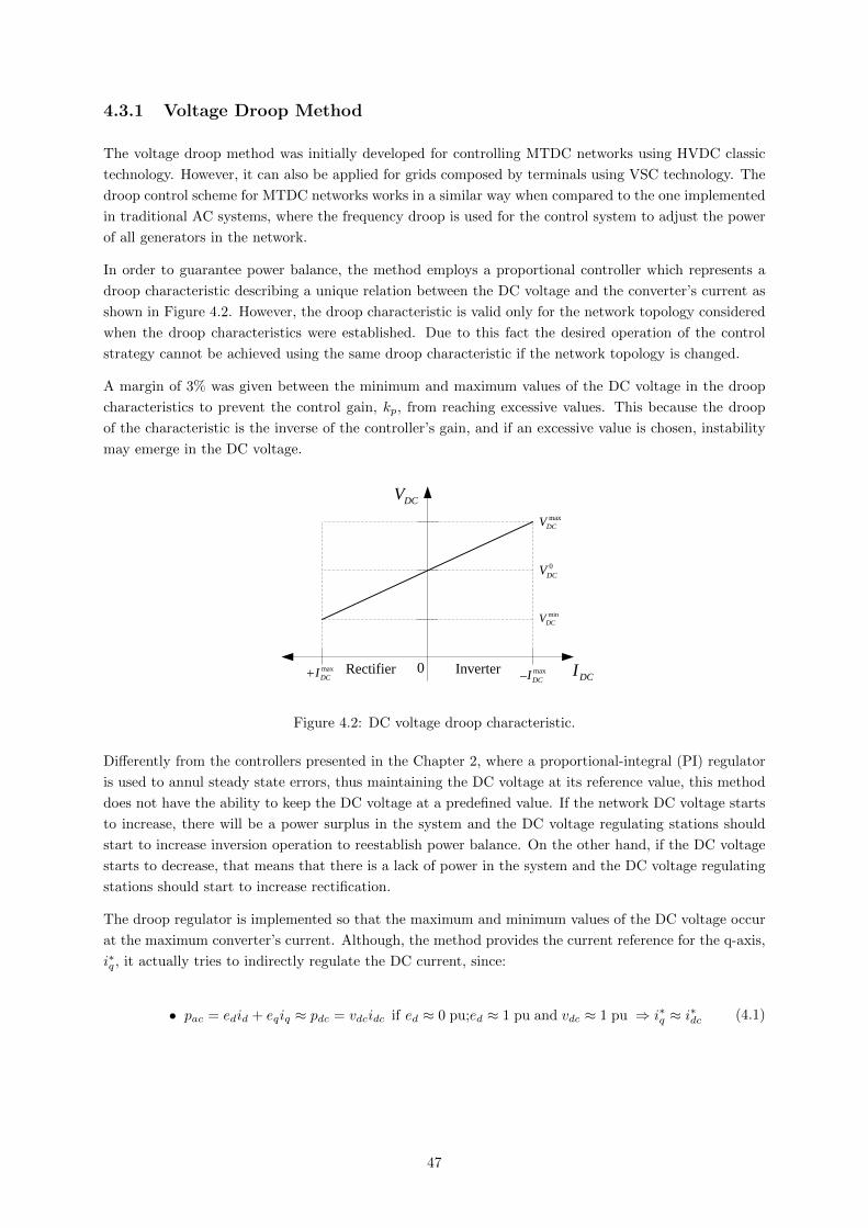
4.3.1 Voltage Droop Method
The voltage droop method was initially developed for controlling MTDC networks using HVDC classic
technology. However, it can also be applied for grids composed by terminals using VSC technology. The
droop control scheme for MTDC networks works in a similar way when compared to the one implemented
in traditional AC systems, where the frequency droop is used for the control system to adjust the power
of all generators in the network.
In order to guarantee power balance, the method employs a proportional controller which represents a
droop characteristic describing a unique relation between the DC voltage and the converter’s current as
shown in Figure 4.2. However, the droop characteristic is valid only for the network topology considered
when the droop characteristics were established. Due to this fact the desired operation of the control
strategy cannot be achieved using the same droop characteristic if the network topology is changed.
A margin of 3% was given between the minimum and maximum values of the DC voltage in the droop
characteristics to prevent the control gain, kp, from reaching excessive values. This because the droop
of the characteristic is the inverse of the controller’s gain, and if an excessive value is chosen, instability
may emerge in the DC voltage.
DCV
InverterRectifier
min
DCV
max
DCV
DCI0 max
DCImax
DCI
0
DCV
Figure 4.2: DC voltage droop characteristic.
Differently from the controllers presented in the Chapter 2, where a proportional-integral (PI) regulator
is used to annul steady state errors, thus maintaining the DC voltage at its reference value, this method
does not have the ability to keep the DC voltage at a predefined value. If the network DC voltage starts
to increase, there will be a power surplus in the system and the DC voltage regulating stations should
start to increase inversion operation to reestablish power balance. On the other hand, if the DC voltage
starts to decrease, that means that there is a lack of power in the system and the DC voltage regulating
stations should start to increase rectification.
The droop regulator is implemented so that the maximum and minimum values of the DC voltage occur
at the maximum converter’s current. Although, the method provides the current reference for the q-axis,
i∗q , it actually tries to indirectly regulate the DC current, since:
• pac = edid + eqiq ≈ pdc = vdcidc if ed ≈ 0 pu;ed ≈ 1 pu and vdc ≈ 1 pu ⇒ i∗q ≈ i∗dc (4.1)
47
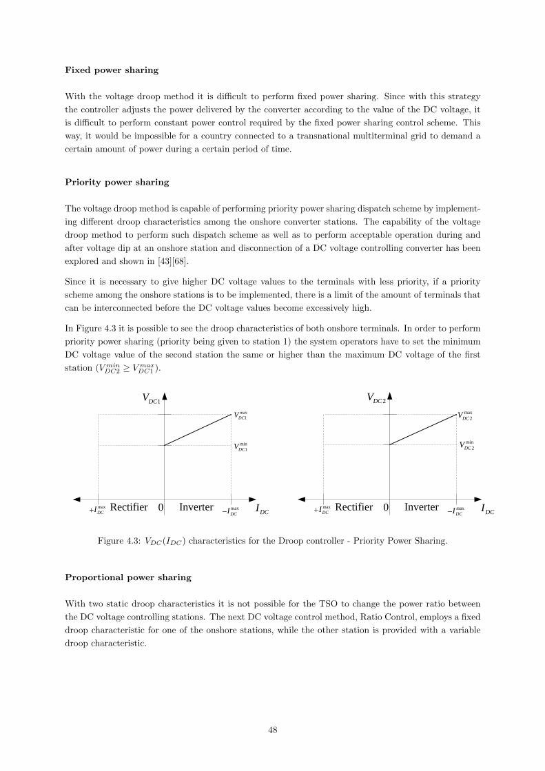
Fixed power sharing
With the voltage droop method it is difficult to perform fixed power sharing. Since with this strategy
the controller adjusts the power delivered by the converter according to the value of the DC voltage, it
is difficult to perform constant power control required by the fixed power sharing control scheme. This
way, it would be impossible for a country connected to a transnational multiterminal grid to demand a
certain amount of power during a certain period of time.
Priority power sharing
The voltage droop method is capable of performing priority power sharing dispatch scheme by implement-
ing different droop characteristics among the onshore converter stations. The capability of the voltage
droop method to perform such dispatch scheme as well as to perform acceptable operation during and
after voltage dip at an onshore station and disconnection of a DC voltage controlling converter has been
explored and shown in [43][68].
Since it is necessary to give higher DC voltage values to the terminals with less priority, if a priority
scheme among the onshore stations is to be implemented, there is a limit of the amount of terminals that
can be interconnected before the DC voltage values become excessively high.
In Figure 4.3 it is possible to see the droop characteristics of both onshore terminals. In order to perform
priority power sharing (priority being given to station 1) the system operators have to set the minimum
DC voltage value of the second station the same or higher than the maximum DC voltage of the first
station (V minDC2 ≥ V maxDC1 ).
1DCV
InverterRectifier
min
1DCV
max
1DCV
DCI0 max
DCImax
DCI
2DCV
InverterRectifier
min
2DCV
max
2DCV
DCI0 max
DCImax
DCI
Figure 4.3: VDC(IDC) characteristics for the Droop controller - Priority Power Sharing.
Proportional power sharing
With two static droop characteristics it is not possible for the TSO to change the power ratio between
the DC voltage controlling stations. The next DC voltage control method, Ratio Control, employs a fixed
droop characteristic for one of the onshore stations, while the other station is provided with a variable
droop characteristic.
48
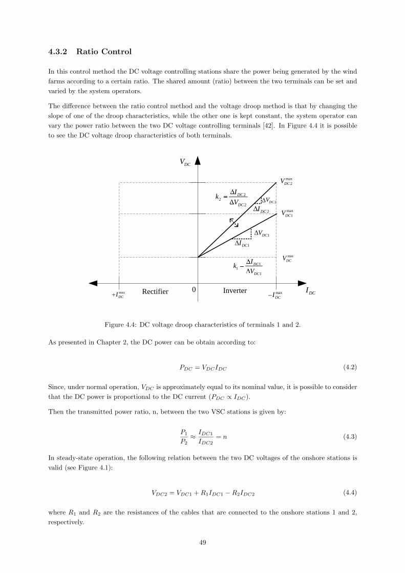
4.3.2 Ratio Control
In this control method the DC voltage controlling stations share the power being generated by the wind
farms according to a certain ratio. The shared amount (ratio) between the two terminals can be set and
varied by the system operators.
The difference between the ratio control method and the voltage droop method is that by changing the
slope of one of the droop characteristics, while the other one is kept constant, the system operator can
vary the power ratio between the two DC voltage controlling terminals [42]. In Figure 4.4 it is possible
to see the DC voltage droop characteristics of both terminals.
DCV
InverterRectifier
min
DCV
max
2DCV
DCI0max
DCImax
DCI
max
1DCV
1DCV
2DCV
1DCI
2DCI
11
1
DC
DC
Ik
V
22
2
DC
DC
Ik
V
Figure 4.4: DC voltage droop characteristics of terminals 1 and 2.
As presented in Chapter 2, the DC power can be obtain according to:
PDC = VDCIDC (4.2)
Since, under normal operation, VDC is approximately equal to its nominal value, it is possible to consider
that the DC power is proportional to the DC current (PDC ∝ IDC).
Then the transmitted power ratio, n, between the two VSC stations is given by:
P1
P2≈ IDC1
IDC2= n (4.3)
In steady-state operation, the following relation between the two DC voltages of the onshore stations is
valid (see Figure 4.1):
VDC2 = VDC1 +R1IDC1 −R2IDC2 (4.4)
where R1 and R2 are the resistances of the cables that are connected to the onshore stations 1 and 2,
respectively.
49
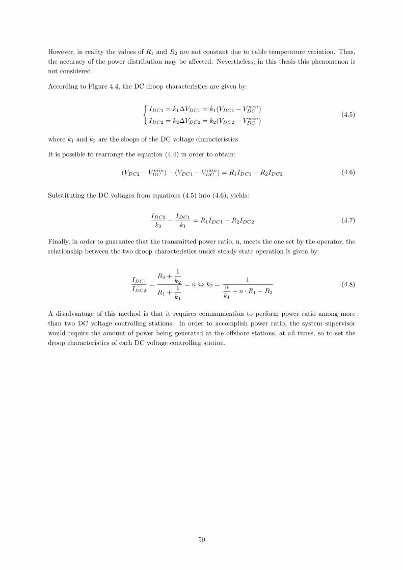
However, in reality the values of R1 and R2 are not constant due to cable temperature variation. Thus,
the accuracy of the power distribution may be affected. Nevertheless, in this thesis this phenomenon is
not considered.
According to Figure 4.4, the DC droop characteristics are given by:
IDC1 = k1∆VDC1 = k1(VDC1 − V minDC )
IDC2 = k2∆VDC2 = k2(VDC2 − V minDC )(4.5)
where k1 and k2 are the sloops of the DC voltage characteristics.
It is possible to rearrange the equation (4.4) in order to obtain:
(VDC2 − V minDC )− (VDC1 − V minDC ) = R1IDC1 −R2IDC2 (4.6)
Substituting the DC voltages from equations (4.5) into (4.6), yields:
IDC2
k2− IDC1
k1= R1IDC1 −R2IDC2 (4.7)
Finally, in order to guarantee that the transmitted power ratio, n, meets the one set by the operator, the
relationship between the two droop characteristics under steady-state operation is given by:
IDC1
IDC2=R2 +
1
k2
R1 +1
k1
= n⇔ k2 =1
n
k1+ n ·R1 −R2
(4.8)
A disadvantage of this method is that it requires communication to perform power ratio among more
than two DC voltage controlling stations. In order to accomplish power ratio, the system supervisor
would require the amount of power being generated at the offshore stations, at all times, so to set the
droop characteristics of each DC voltage controlling station.
50

4.3.3 Priority Control
The priority control is a modified way of using DC voltage droop controllers to perform priority power
sharing. In this control strategy, one onshore terminal will have priority in terms of transmitting the
power generated by the offshore wind farms over the other terminal. The terminal with the highest
priority will control the DC voltage, by means of a PI regulator (see Chapter 2), until it reaches its rated
capacity or a maximum power set point established by system operators. On the other hand, the second
terminal employs a fixed DC voltage droop controller and it will receive the power surplus that could not
be transmitted to the first terminal [42]. The DC voltage controllers are depicted in Figure 4.5.
2DCV
InverterRectifier
max
2DCV
DCI0 max
DCImax
DCI
min
2DCV
1DCV
0maxP
minP
*
1DCV
Figure 4.5: VDC(P ) characteristic of terminal 1 and DC voltage droop characteristic of terminal 2.
If the total generated power by the offshore wind farms is lower than the rated power of the priority
terminal, the DC voltage will be controlled at the predefined value and no power will flow through the
second onshore station. However, if the total generated active power exceeds the power limit of the
first terminal, it will no longer be capable of controlling the DC voltage in the MTDC network. As a
consequence of the power unbalance, the DC voltage inside the system will start to increase.
Under such condition, the terminal using the droop control method is designed to transmit the extra
power. To perform such dispatch scheme, the system operators need to set V minDC2 the same or higher
than the peak value of station 1 during changes of operating point. The values for the DC voltage droop
control have to take into account the grid characteristics, e.g. DC cable resistance variation and DC
voltage dynamic peak values, in order to assure that the second terminal will only transmit power when
the limit is reached in the first one. Moreover, system design rules, such as the DC voltage ratings of the
VSC stations and of the DC cables have also to be taken into consideration [43].
51

4.3.4 Voltage Margin Method
The basic control strategy of the voltage margin method consists of a DC voltage controller with a limiter
at its output as shown in Figure 4.6. The DC voltage controller employs a PI controller (see Chapter
2). The limiter is applied to limit the q-axis current reference value to an upper value and a lower value,
in order to prevent overcurrents in the converter valves. Thus, the active power flowing through the
converter is also limited to an upper and a lower value. This way, the DC voltage controller will be
able to keep the DC voltage equal to the reference value as long as the active power flowing through the
converter is between the predefined limits.
*
qi
DCv
*
Cw
Cw
*
Cw,
,
i w
p w
kk
s
2x1
2C
*
,q upperi
*
,q loweri
Figure 4.6: DC voltage controller and limiter present in the Voltage Margin Method.
As previously presented in Chapter 2, the active power flowing through the converter can be obtained
by:
pac = edid + eqiq (4.9)
Therefore, the relationship between the lower limit of the q-axis current reference value and the converter’s
inversion limit is given by:
i∗q,lower =plower − ed · i∗d
eq(4.10)
On the other hand, the upper limit of the q-axis current reference value is calculated as:
i∗q,upper =pupper − ed · i∗d
eq(4.11)
where i∗d is the d-axis current reference value provided by the reactive channel outer controllers; ed and eq
are the PCC voltages in the (dq) frame; and Plower and Pupper are, respectively, the converter’s inversion
and rectification limits. In Figure 4.7 it is shown the complete one-stage DC voltage controller.
The lower and upper values of the limiter are adjustable and may be set directly at the converter station
or sent from a remote supervisory dispatch controller. By adjusting the lower and upper limits to the
same value, the converter can perform constant power control and therefore, act as a passive constant
load [46]. It is important to notice that the converter will not be able to control the DC voltage when
the active power flowing through the converter exceeds the limits. Thus, if the converter is performing
rectification and the active power exceeds Pmax (see Figure 4.8) the DC voltage will drop since the
converter has reached its rated power. On the other hand, if inversion is being performed at the station
and if the power surpasses Pmin the DC voltage will increase, since the converter will no longer be able
to remove the required amount of energy from the system.
The characteristic presented in Figure 4.8 shows that the converter will keep the DC voltage equal to the
reference value (B-C-D part of the presented voltage characteristic) as long as the active power flowing
through the converter is kept between the limits. The converter will perform inversion when the operation
point is in the B-C line and rectification when the operation point is in the C-D line.
52
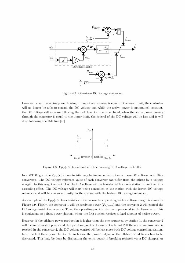
*
qi*
Cw
Cw
*
Cw ,
,
i w
p w
kk
s
2x1
2C
*
,q upperi
*
,q loweri
lowerp
qe
DCv
de*
di
upperp
qe
de*
di
DC voltage controller
Figure 4.7: One-stage DC voltage controller.
However, when the active power flowing through the converter is equal to the lower limit, the controller
will no longer be able to control the DC voltage and while the active power is maintained constant,
the DC voltage will increase following the B-A line. On the other hand, when the active power flowing
through the converter is equal to the upper limit, the control of the DC voltage will be lost and it will
drop following the D-E line [45].
DCV
Inverter Rectifier0maxP
minP upperPlowerP
A
BC D
E
Figure 4.8: VDC(P ) characteristic of the one-stage DC voltage controller.
In a MTDC grid, the VDC(P ) characteristic may be implemented in two or more DC voltage controlling
converters. The DC voltage reference value of each converter can differ from the others by a voltage
margin. In this way, the control of the DC voltage will be transferred from one station to another in a
cascading effect. The DC voltage will start being controlled at the station with the lowest DC voltage
reference and will be controlled, lastly, in the station with the highest DC voltage reference.
An example of the VDC(P ) characteristics of two converters operating with a voltage margin is shown in
Figure 4.9. Firstly, the converter 1 will be receiving power (P1,lower) and the converter 2 will control the
DC voltage inside the network. Thus, the operating point is the one represented in the figure as P. This
is equivalent as a fixed power sharing, where the first station receives a fixed amount of active power.
However, if the offshore power production is higher than the one requested by station 1, the converter 2
will receive this extra power and the operation point will move to the left of P. If the maximum inversion is
reached in the converter 2, the DC voltage control will be lost since both DC voltage controlling stations
have reached their power limits. In such case the power output of the offshore wind farms has to be
decreased. This may be done by dissipating the extra power in breaking resistors via a DC chopper, or
53

2DCV
02, ,1upperP
2, ,1lowerP
1DCV
01, ,1upperP1, ,1lowerP
DCV
01, ,1upperP
2, ,1lowerP1, ,1lowerP 2, ,1upperP
Converter 1 Converters 1 and 2Converter 2
Pmargin
*
1DCV*
2DCV
Figure 4.9: VDC(P ) characteristics for two one-stage DC voltage controlling converters and the resultingoperating point (P).
through fast reduction of the wind farms output power [48].
The voltage margin method is the only control strategy capable of performing fixed, priority and pro-
portional power sharing, making this method a versatile and powerful control scheme [34]. However, in
order to perform the different power schemes, it is necessary to implement a voltage margin method that
employs more than one DC voltage stage.
Two-stages DC voltage controller
In order to achieve a more versatile and robust voltage margin method, a two-stage DC voltage controller
may be applied. In this approach, as shown in Figure 4.10, two proportional-integral controllers are used
[34][46].
When the VSC terminal tries to control the DC voltage at the first stage the DC voltage controller 1 is
used. On the other hand, when the station is controlling the DC voltage at the second stage a new PI
controller is employed (DC voltage controller 2). In Figure 4.10 it is possible to observe how these PI
controllers are interconnected and Figure 4.11 shows the VDC(P ) characteristic of the station and how it
is achieved.
Figure 4.12 shows an example of a station using the two-stage voltage margin method. This controller is
helpful when the second converter has reached its inversion limit. In this way, the DC voltage will start
to increase due to the power imbalance (G-H line). Converter 1 will control the DC voltage using the
second PI controller at V ∗DC1,H .
The DC reference value of the second PI controller is set higher than the one of the first controller. Thus,
the first controller will maintain the DC voltage equal to its reference value and perform operation in the
first stage (D-E line) and when the DC voltage rises above the reference value of the second controller, it
will automatically increase its inversion capability and will start controlling the DC voltage at the second
stage. The operation point will then be situated in the B-C line.
Fixed power sharing
When in a fixed power sharing dispatch scheme, the VDC(P ) characteristics of the stations have to set by
the TSO as presented in Figure 4.13. With such DC voltage controller, station 1 will act as a constant
passive load absorbing a certain amount of active power, P1,lower,1. On the other hand, station 2 will be
responsible for controlling the DC voltage inside the MTDC grid.
54

*
qi*
Cw
Cw
,
,
i w
p w
kk
s
2x1
2C
*
, ,1q upperi
*
, ,1q loweriDCv
,1upperp
qe
de*
di
DC voltage controller 1
*
,C Hw
Cw
*
Cw,
,
i w
p w
kk
s
2x1
2C
DC voltage controller 2
*
, ,2q upperi
,2upperp
qe
de*
di
*
, ,2q loweri
,2lowerp
qe
de*
di
*
Cw
Figure 4.10: Two-stage DC voltage controller.
DCV
0,1upperP,2lowerP0
,1upperP
,1 ,2lower upperP P
0,2lowerP
,2upperP
DCVDCV
* (first stage)DCV
*
, (second stage)DC HV
A
BC
D
C
D E
F
A
B C
D E
F
,1lowerP
Figure 4.11: VDC(P ) characteristic of a station composed by two stages.
2DCV
02,upperP
2,lowerP
1DCV
0
Converter 1 Converter 2
*
1,DC HV*
2DCV
DCV
01, ,1upperP1, ,2lowerP
E
2,upperP1, ,2lowerP
*
1DCV
A
BC
D
F
G
HI
J
1, ,1 1, ,2lower upperP P 1, ,1upperP
Converters 1 and 2
P
2,lowerP
Figure 4.12: VDC(P ) characteristics for two DC voltage controlling converters and the resulting operatingpoint (P).
55
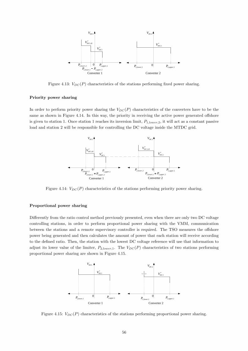
2DCV
02, ,1upperP
1DCV
0
Converter 1 Converter 2
*
2DCV
1, ,1upperP1, ,2lowerP
1, ,1 1, ,2lower upperP P2, ,1lowerP
*
1DCV
*
1,DC HV
Figure 4.13: VDC(P ) characteristics of the stations performing fixed power sharing.
Priority power sharing
In order to perform priority power sharing the VDC(P ) characteristics of the converters have to be the
same as shown in Figure 4.14. In this way, the priority in receiving the active power generated offshore
is given to station 1. Once station 1 reaches its inversion limit, P1,lower,2, it will act as a constant passive
load and station 2 will be responsible for controlling the DC voltage inside the MTDC grid.
2DCV
0
Converter 2
2, ,1upperP2, ,2lowerP
2, ,1 2, ,2lower upperP P
*
2,DC HV
*
2DCV
1DCV
0
1, ,1 1, ,2lower upperP P1, ,2lowerP
*
1DCV
*
1,DC HV
1, ,1upperP
Converter 1
Figure 4.14: VDC(P ) characteristics of the stations performing priority power sharing.
Proportional power sharing
Differently from the ratio control method previously presented, even when there are only two DC voltage
controlling stations, in order to perform proportional power sharing with the VMM, communication
between the stations and a remote supervisory controller is required. The TSO measures the offshore
power being generated and then calculates the amount of power that each station will receive according
to the defined ratio. Then, the station with the lowest DC voltage reference will use that information to
adjust its lower value of the limiter, P2,lower,1. The VDC(P ) characteristics of two stations performing
proportional power sharing are shown in Figure 4.15.
2DCV
02, ,1upperP
2, ,1lowerP
1DCV
01, ,1upperP
1, ,1lowerP
Converter 1 Converter 2
*
1DCV *
2DCV
Figure 4.15: VDC(P ) characteristics of the stations performing proportional power sharing.
56
Chapter 5
Simulation Results and Discussion
5.1 Introduction
In this chapter the results of the computer simulations performed using the software MATLAB/Simulink
are presented and discussed in order to evaluate and validate the developed models and control structures.
The VSC control system (i.e. inner current controller and outer controllers) is analyzed and tested
in order to see if the performance of the system is as expected. Simulations using the implemented
DC voltage control strategies are presented and discussed. It is shown the capability of the different DC
voltage control strategies of performing different market dispatch schemes (fixed, priority and proportional
power sharing) during normal operation. The developed model for the MTDC grid shown in Chapter 3
is used for all the simulations.
It is important to refer that, the outer controllers chosen for the onshore converters were the DC voltage
controller for the active channel and the reactive power controller for the reactive channel. On the other
hand, the offshore converter stations were set to control the active power and the amplitude of the PCC
voltage.
For every simulation it is shown a chart with the DC voltage, active power, module of the voltage at the
PCC, reactive power, module of the converter’s voltage, and the module of the converter’s current. All
the mentioned AC quantities are presented in the (dq) frame. The charts display the information for all
the converter stations and the results are shown in pu.
All the results are plotted using the same axis values for the analyzed dispatch schemes and DC voltage
control strategies. This may not be the better solution for a particular study case but it provides an
important tool to easily and quickly compare the results obtained from the different case scenarios.
In the last part of the present chapter, the VSC-HVDC transmission model and control system are
analyzed by submitting them to AC fault situations. The most common and demanding fault scenarios,
the single-line-to-ground fault and the three-phase fault are simulated in order to test the capability of
the VSC-HVDC model to return to the previous steady-state time shortly after the fault is cleared.
57
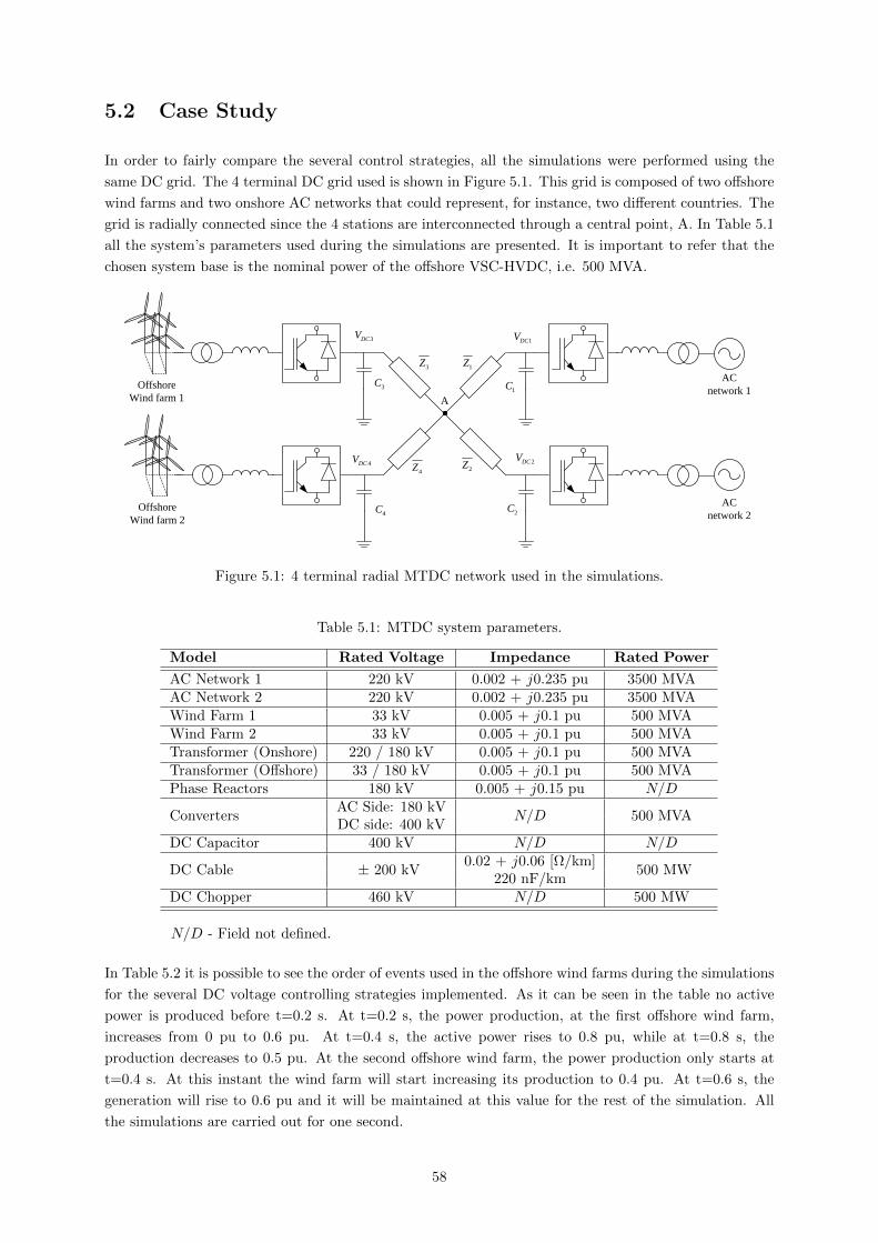
5.2 Case Study
In order to fairly compare the several control strategies, all the simulations were performed using the
same DC grid. The 4 terminal DC grid used is shown in Figure 5.1. This grid is composed of two offshore
wind farms and two onshore AC networks that could represent, for instance, two different countries. The
grid is radially connected since the 4 stations are interconnected through a central point, A. In Table 5.1
all the system’s parameters used during the simulations are presented. It is important to refer that the
chosen system base is the nominal power of the offshore VSC-HVDC, i.e. 500 MVA.
AC
network 1
AC
network 24C
1Z3Z
2Z4Z
3C
2C
1C
1DCV
2DCV4DCV
3DCV
A
Offshore
Wind farm 1
Offshore
Wind farm 2
Figure 5.1: 4 terminal radial MTDC network used in the simulations.
Table 5.1: MTDC system parameters.
Model Rated Voltage Impedance Rated Power
AC Network 1 220 kV 0.002 + j0.235 pu 3500 MVAAC Network 2 220 kV 0.002 + j0.235 pu 3500 MVAWind Farm 1 33 kV 0.005 + j0.1 pu 500 MVAWind Farm 2 33 kV 0.005 + j0.1 pu 500 MVATransformer (Onshore) 220 / 180 kV 0.005 + j0.1 pu 500 MVATransformer (Offshore) 33 / 180 kV 0.005 + j0.1 pu 500 MVAPhase Reactors 180 kV 0.005 + j0.15 pu N/D
ConvertersAC Side: 180 kV
N/D 500 MVADC side: 400 kV
DC Capacitor 400 kV N/D N/D
DC Cable ± 200 kV0.02 + j0.06 [Ω/km]
500 MW220 nF/km
DC Chopper 460 kV N/D 500 MW
N/D - Field not defined.
In Table 5.2 it is possible to see the order of events used in the offshore wind farms during the simulations
for the several DC voltage controlling strategies implemented. As it can be seen in the table no active
power is produced before t=0.2 s. At t=0.2 s, the power production, at the first offshore wind farm,
increases from 0 pu to 0.6 pu. At t=0.4 s, the active power rises to 0.8 pu, while at t=0.8 s, the
production decreases to 0.5 pu. At the second offshore wind farm, the power production only starts at
t=0.4 s. At this instant the wind farm will start increasing its production to 0.4 pu. At t=0.6 s, the
generation will rise to 0.6 pu and it will be maintained at this value for the rest of the simulation. All
the simulations are carried out for one second.
58

Table 5.2: Order of events in the offshore wind farms.
Time [s] 0 0.2 0.4 0.6 0.8
WF 1 Power [pu] 0 0.6 0.8 0.8 0.5WF 2 Power [pu] 0 0 0.4 0.6 0.6
AC faults
AC faults will be simulated at onshore and offshore stations. Firstly, a three-phase AC fault at one of
the DC voltage controlling stations will be simulated, presented and analyzed. Secondly, an one-phase
AC fault will be simulated, once again, at one of the onshore stations. Lastly, a three-phase AC fault
will be simulated at one of the offshore wind farms.
In Table 5.3 it is possible to see the order of events used in the offshore wind farms during these simulations.
As it can be seen in the table, no active power is produced before t=0.1 s. At t=0.1 s, the power
production, at both offshore wind farms, increases from 0 pu to 0.6 pu. At t=0.4 s, the active power
being generated at the offshore wind farms is reduced by means of a fast reduction control method to 0.3
pu [48]. However, at t=0.6 s, the production is reestablish to the same value it had before the fault, being
0.6 pu generated at each wind farm, and it will be maintained at this value for the rest of the simulation.
All the simulations are carried out for one second. The simulated faults occur at t=0.3 s and are cleared
at t=0.5 s.
Table 5.3: Order of events in the offshore wind farms (fault scenario).
Time [s] 0 0.1 0.4 0.6
WF 1 Power [pu] 0 0.6 0.3 0.6WF 2 Power [pu] 0 0.6 0.3 0.6
59

5.3 Simulation Results
In these simulations the controllers described in Chapter 2 were applied for the inner current controller
and the outer controllers. However, the DC voltage controller is different for each simulation in order to
compare the performance and capability of the several developed DC voltage controllers to perform the
different market dispatch schemes.
5.3.1 Voltage Droop Method
In this simulation the voltage droop method with fixed droop characteristics will be employed in both
onshore stations. With this control method, as previously explained, it is possible to implement the
priority power sharing dispatch scheme.
Priority Power Sharing
In order to perform this dispatch scheme the DC voltage controllers displayed in Figure 5.2 were employed.
Priority in receiving the power generated offshore was given to station 1. Therefore, station 1 will start
receiving power when its DC voltage is higher than 1 pu and it will reach its rated power when its
DC voltage is 1.03 pu. On the other hand, the second station will only start to transmit power when
VDC2=1.04 pu and, therefore, station 1 will have already reached its rated power. Station 2 will reach
its rated power when it has a DC voltage of 1.07 pu.
A margin of 3% was given between the minimum and maximum values of the DC voltage in the droop
characteristics to prevent the control gain, kp, from reaching excessive values. This is because the slope
of the characteristic is the inverse of the controller’s gain and if an excessive value is chosen, instability
may arise in the DC voltage.
2DCV
InverterRectifier
min
2DCV
max
2DCV
DCI0 max
DCImax
DCI
1DCV
InverterRectifier
min
1DCV
max
1DCV
DCI0 max
DCImax
DCI
1.00
1.031.04
1.07
Converter 1 Converter 2
Figure 5.2: VDC(IDC) characteristics for the droop controller - Priority Power Sharing.
The simulation results in Figure 5.3 show that a priority scheme is applied among the onshore stations as
desired. Initially there is no active power being generated at the offshore wind farms. However, at t=0.2
s the wind farm 1 starts to transmit power to the grid. Therefore, the DC voltage inside the grid starts
to increase. As it can be seen in the DC voltage chart (Figure 5.3 (a)), the first station starts to transmit
power to reestablish the power balance. When station 1 reaches its rated power, around t=0.4 s, station
2 starts to receive power. From t=0.4 s until the end of the simulation, station 1 keeps its transmission
in 1 pu and station 2 is the one responsible to keep the power balance inside the grid. This way it will
deal with the variability in the power generation at the offshore wind farms. The stations are not able
60
to keep the DC voltage at its nominal value since DC voltage droop characteristics, i.e. proportional
control, were employed.
In the AC voltage at PCC chart (Figure 5.3 (c)) it is possible to observe that at the wind farms this
value is kept equal to its reference, 1 pu, while at the onshore stations this value varies with time since
the converter stations are not controlling the AC voltage. Thus, the PCC voltage changes due to the
fact that the stations are controlling the power factor at unity. In order to perform this control the
onshore stations need to change the PCC voltage of the converters to values that annul the reactive
power exchanged with their AC network. This way it is possible to see in the forth chart (Figure 5.3 (d))
that the reactive power is controlled at 0 pu in the onshore stations, while at the wind farms that does
not occur. However, as it can be seen the reactive power exchanged is always lower than 0.1 pu during
the complete simulation time.
One additional remark is that in the converter’s current chart (Figure 5.3 (f)) station 1 is receiving 1 pu
of power but its converter’s current is slightly higher than 1 pu. This is due to the fact that the power
is being controlled at the PCC and this voltage is not being controlled (the converter’s reactive power is
being controlled instead) and as it can be seen in Figure 5.3 (c) it is lower than 1 pu. On the other hand,
the power being received is 1 pu and so the converter’s current has to compensate for this difference.
However, the overcurrent is less than 0.05 pu, which, momentarily, do not pose a threat to the converter
IGBT valves.
61

0 0.1 0.2 0.3 0.4 0.5 0.6 0.7 0.8 0.9 10.97
0.98
0.99
1
1.01
1.02
1.03
1.04
1.05
1.06
1.07
1.08
time [s]
Vdc
[pu]
DC Voltage at the VSC stations
VSC 1VSC 2WF 1WF 2
0 0.1 0.2 0.3 0.4 0.5 0.6 0.7 0.8 0.9 1-1.2
-1
-0.8
-0.6
-0.4
-0.2
0
0.2
0.4
0.6
0.8
1
1.2
time [s]
Pdc
[pu]
Active Power at the VSC stations
VSC 1VSC 2WF 1WF 2
0 0.1 0.2 0.3 0.4 0.5 0.6 0.7 0.8 0.9 10.95
0.96
0.97
0.98
0.99
1
1.01
1.02
1.03
1.04
1.05
1.06
time [s]
|Vac
| [pu
]
AC Voltage at PCC
VSC 1VSC 2WF 1WF 2
0 0.1 0.2 0.3 0.4 0.5 0.6 0.7 0.8 0.9 1-0.15
-0.1
-0.05
0
0.05
0.1
0.15
time [s]
Qac
[pu]
Reactive Power at the VSC stations
VSC 1VSC 2WF 1WF 2
0 0.1 0.2 0.3 0.4 0.5 0.6 0.7 0.8 0.9 10.92
0.94
0.96
0.98
1
1.02
1.04
1.06
1.08
1.1
1.12
time [s]
|vc_
dq| [
pu]
Converter's AC Voltage
VSC 1VSC 2WF 1WF 2
0 0.1 0.2 0.3 0.4 0.5 0.6 0.7 0.8 0.9 1-0.1
0
0.1
0.2
0.3
0.4
0.5
0.6
0.7
0.8
0.9
1
1.1
time [s]
|ic_d
q| [p
u]
Converter's AC Current
VSC 1VSC 2WF 1WF 2
Figure 5.3: Simulation results using the DC Voltage Droop Method - Priority Power Sharing.
62
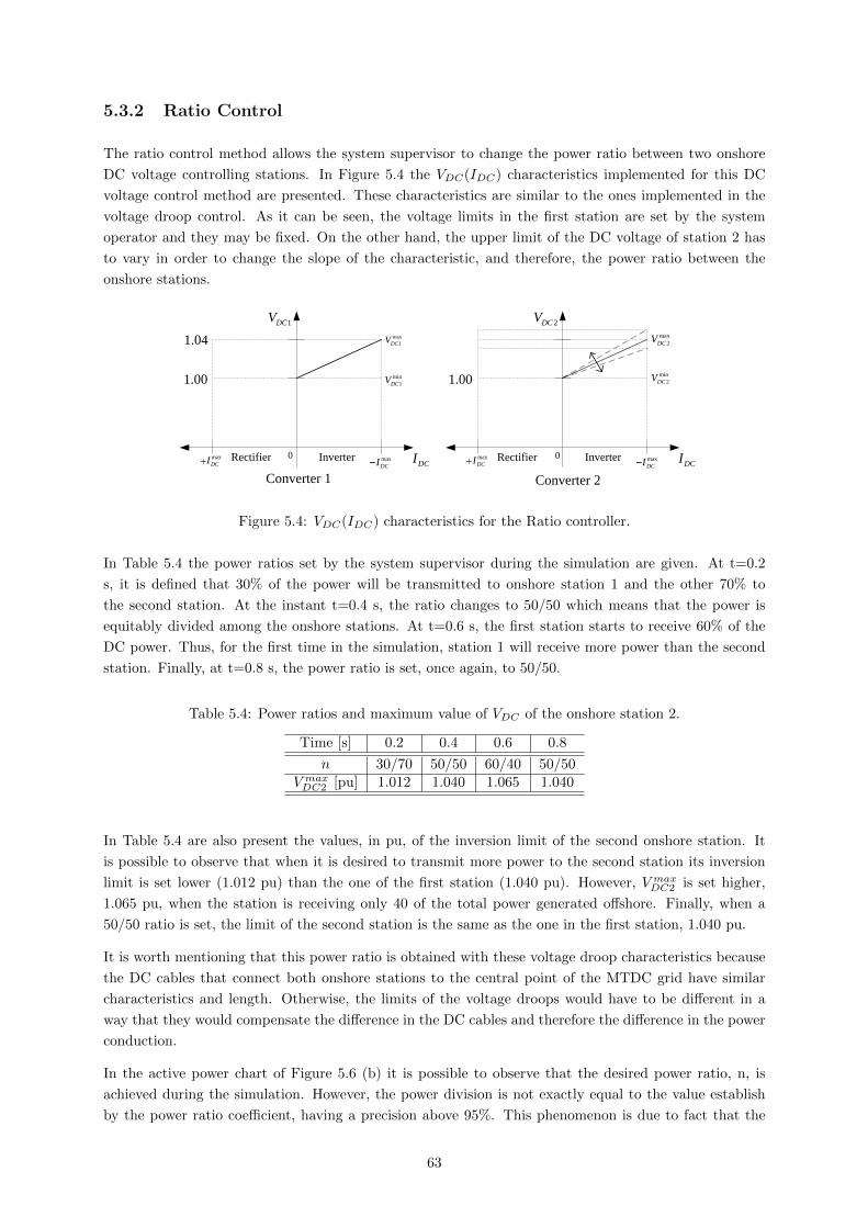
5.3.2 Ratio Control
The ratio control method allows the system supervisor to change the power ratio between two onshore
DC voltage controlling stations. In Figure 5.4 the VDC(IDC) characteristics implemented for this DC
voltage control method are presented. These characteristics are similar to the ones implemented in the
voltage droop control. As it can be seen, the voltage limits in the first station are set by the system
operator and they may be fixed. On the other hand, the upper limit of the DC voltage of station 2 has
to vary in order to change the slope of the characteristic, and therefore, the power ratio between the
onshore stations.
2DCV
InverterRectifier
min
2DCV
max
2DCV
DCImax
DCImax
DCI
1DCV
InverterRectifier
min
1DCV
max
1DCV
DCI0 max
DCImax
DCI
1.00
1.04
1.00
Converter 1 Converter 2
0
Figure 5.4: VDC(IDC) characteristics for the Ratio controller.
In Table 5.4 the power ratios set by the system supervisor during the simulation are given. At t=0.2
s, it is defined that 30% of the power will be transmitted to onshore station 1 and the other 70% to
the second station. At the instant t=0.4 s, the ratio changes to 50/50 which means that the power is
equitably divided among the onshore stations. At t=0.6 s, the first station starts to receive 60% of the
DC power. Thus, for the first time in the simulation, station 1 will receive more power than the second
station. Finally, at t=0.8 s, the power ratio is set, once again, to 50/50.
Table 5.4: Power ratios and maximum value of VDC of the onshore station 2.
Time [s] 0.2 0.4 0.6 0.8
n 30/70 50/50 60/40 50/50V maxDC2 [pu] 1.012 1.040 1.065 1.040
In Table 5.4 are also present the values, in pu, of the inversion limit of the second onshore station. It
is possible to observe that when it is desired to transmit more power to the second station its inversion
limit is set lower (1.012 pu) than the one of the first station (1.040 pu). However, V maxDC2 is set higher,
1.065 pu, when the station is receiving only 40 of the total power generated offshore. Finally, when a
50/50 ratio is set, the limit of the second station is the same as the one in the first station, 1.040 pu.
It is worth mentioning that this power ratio is obtained with these voltage droop characteristics because
the DC cables that connect both onshore stations to the central point of the MTDC grid have similar
characteristics and length. Otherwise, the limits of the voltage droops would have to be different in a
way that they would compensate the difference in the DC cables and therefore the difference in the power
conduction.
In the active power chart of Figure 5.6 (b) it is possible to observe that the desired power ratio, n, is
achieved during the simulation. However, the power division is not exactly equal to the value establish
by the power ratio coefficient, having a precision above 95%. This phenomenon is due to fact that the
63
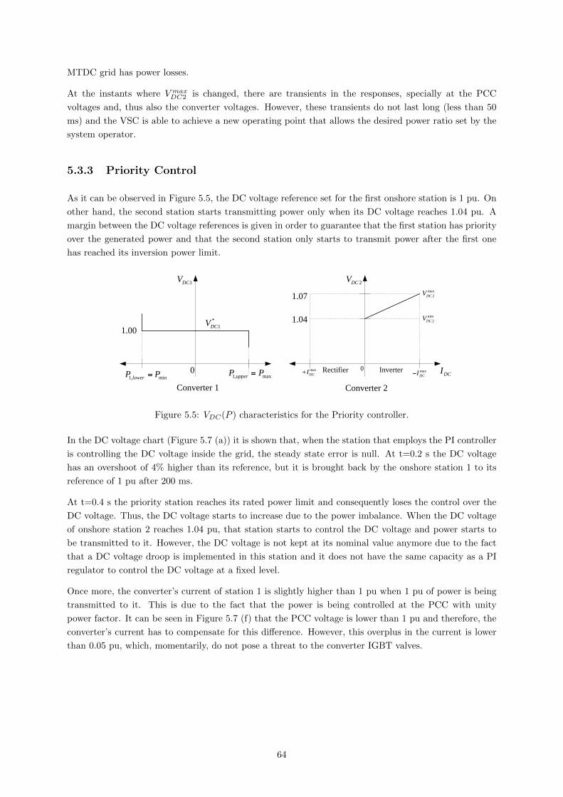
MTDC grid has power losses.
At the instants where V maxDC2 is changed, there are transients in the responses, specially at the PCC
voltages and, thus also the converter voltages. However, these transients do not last long (less than 50
ms) and the VSC is able to achieve a new operating point that allows the desired power ratio set by the
system operator.
5.3.3 Priority Control
As it can be observed in Figure 5.5, the DC voltage reference set for the first onshore station is 1 pu. On
other hand, the second station starts transmitting power only when its DC voltage reaches 1.04 pu. A
margin between the DC voltage references is given in order to guarantee that the first station has priority
over the generated power and that the second station only starts to transmit power after the first one
has reached its inversion power limit.
2DCV
InverterRectifier
min
2DCV
max
2DCV
DCI0 max
DCImax
DCI
1.04
1.07
Converter 2
1DCV
01, maxupperP P
1, minlowerP P
Converter 1
*
1DCV1.00
Figure 5.5: VDC(P ) characteristics for the Priority controller.
In the DC voltage chart (Figure 5.7 (a)) it is shown that, when the station that employs the PI controller
is controlling the DC voltage inside the grid, the steady state error is null. At t=0.2 s the DC voltage
has an overshoot of 4% higher than its reference, but it is brought back by the onshore station 1 to its
reference of 1 pu after 200 ms.
At t=0.4 s the priority station reaches its rated power limit and consequently loses the control over the
DC voltage. Thus, the DC voltage starts to increase due to the power imbalance. When the DC voltage
of onshore station 2 reaches 1.04 pu, that station starts to control the DC voltage and power starts to
be transmitted to it. However, the DC voltage is not kept at its nominal value anymore due to the fact
that a DC voltage droop is implemented in this station and it does not have the same capacity as a PI
regulator to control the DC voltage at a fixed level.
Once more, the converter’s current of station 1 is slightly higher than 1 pu when 1 pu of power is being
transmitted to it. This is due to the fact that the power is being controlled at the PCC with unity
power factor. It can be seen in Figure 5.7 (f) that the PCC voltage is lower than 1 pu and therefore, the
converter’s current has to compensate for this difference. However, this overplus in the current is lower
than 0.05 pu, which, momentarily, do not pose a threat to the converter IGBT valves.
64
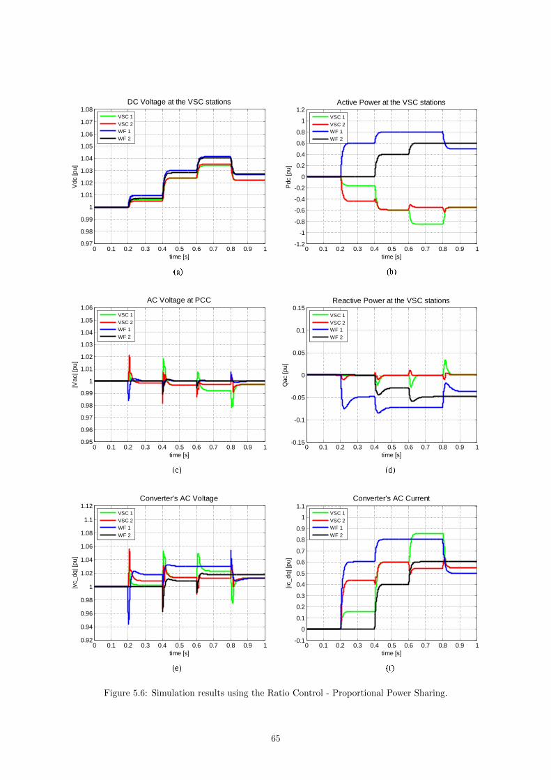
0 0.1 0.2 0.3 0.4 0.5 0.6 0.7 0.8 0.9 10.97
0.98
0.99
1
1.01
1.02
1.03
1.04
1.05
1.06
1.07
1.08
time [s]
Vdc
[pu]
DC Voltage at the VSC stations
VSC 1VSC 2WF 1WF 2
0 0.1 0.2 0.3 0.4 0.5 0.6 0.7 0.8 0.9 1-1.2
-1
-0.8
-0.6
-0.4
-0.2
0
0.2
0.4
0.6
0.8
1
1.2
time [s]
Pdc
[pu]
Active Power at the VSC stations
VSC 1VSC 2WF 1WF 2
0 0.1 0.2 0.3 0.4 0.5 0.6 0.7 0.8 0.9 10.95
0.96
0.97
0.98
0.99
1
1.01
1.02
1.03
1.04
1.05
1.06
time [s]
|Vac
| [pu
]
AC Voltage at PCC
VSC 1VSC 2WF 1WF 2
0 0.1 0.2 0.3 0.4 0.5 0.6 0.7 0.8 0.9 1-0.15
-0.1
-0.05
0
0.05
0.1
0.15
time [s]
Qac
[pu]
Reactive Power at the VSC stations
VSC 1VSC 2WF 1WF 2
0 0.1 0.2 0.3 0.4 0.5 0.6 0.7 0.8 0.9 10.92
0.94
0.96
0.98
1
1.02
1.04
1.06
1.08
1.1
1.12
time [s]
|vc_
dq| [
pu]
Converter's AC Voltage
VSC 1VSC 2WF 1WF 2
0 0.1 0.2 0.3 0.4 0.5 0.6 0.7 0.8 0.9 1-0.1
0
0.1
0.2
0.3
0.4
0.5
0.6
0.7
0.8
0.9
1
1.1
time [s]
|ic_d
q| [p
u]
Converter's AC Current
VSC 1VSC 2WF 1WF 2
Figure 5.6: Simulation results using the Ratio Control - Proportional Power Sharing.
65

0 0.1 0.2 0.3 0.4 0.5 0.6 0.7 0.8 0.9 10.97
0.98
0.99
1
1.01
1.02
1.03
1.04
1.05
1.06
1.07
1.08
time [s]
Vdc
[pu]
DC Voltage at the VSC stations
VSC 1VSC 2WF 1WF 2
0 0.1 0.2 0.3 0.4 0.5 0.6 0.7 0.8 0.9 1-1.2
-1
-0.8
-0.6
-0.4
-0.2
0
0.2
0.4
0.6
0.8
1
1.2
time [s]
Pdc
[pu]
Active Power at the VSC stations
VSC 1VSC 2WF 1WF 2
0 0.1 0.2 0.3 0.4 0.5 0.6 0.7 0.8 0.9 10.95
0.96
0.97
0.98
0.99
1
1.01
1.02
1.03
1.04
1.05
1.06
time [s]
|Vac
| [pu
]
AC Voltage at PCC
VSC 1VSC 2WF 1WF 2
0 0.1 0.2 0.3 0.4 0.5 0.6 0.7 0.8 0.9 1-0.15
-0.1
-0.05
0
0.05
0.1
0.15
time [s]
Qac
[pu]
Reactive Power at the VSC stations
VSC 1VSC 2WF 1WF 2
0 0.1 0.2 0.3 0.4 0.5 0.6 0.7 0.8 0.9 10.92
0.94
0.96
0.98
1
1.02
1.04
1.06
1.08
1.1
1.12
time [s]
|vc_
dq| [
pu]
Converter's AC Voltage
VSC 1VSC 2WF 1WF 2
0 0.1 0.2 0.3 0.4 0.5 0.6 0.7 0.8 0.9 1-0.1
0
0.1
0.2
0.3
0.4
0.5
0.6
0.7
0.8
0.9
1
1.1
time [s]
|ic_d
q| [p
u]
Converter's AC Current
VSC 1VSC 2WF 1WF 2
Figure 5.7: Simulation results using the Priority Control - Priority Power Sharing.
66
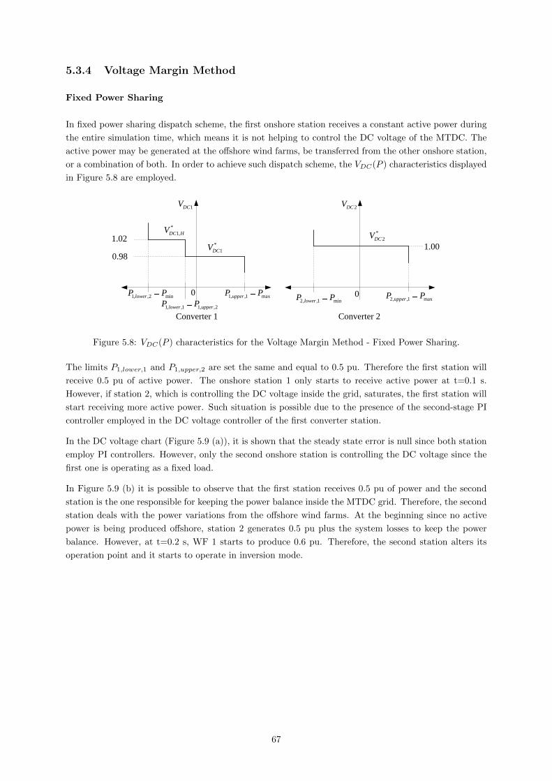
5.3.4 Voltage Margin Method
Fixed Power Sharing
In fixed power sharing dispatch scheme, the first onshore station receives a constant active power during
the entire simulation time, which means it is not helping to control the DC voltage of the MTDC. The
active power may be generated at the offshore wind farms, be transferred from the other onshore station,
or a combination of both. In order to achieve such dispatch scheme, the VDC(P ) characteristics displayed
in Figure 5.8 are employed.
2DCV
02, ,1 maxupperP P
1DCV
0
Converter 1 Converter 2
*
2DCV
1, ,1 maxupperP P1, ,2 minlowerP P
1, ,1 1, ,2lower upperP P2, ,1 minlowerP P
*
1DCV
*
1,DC HV
0.98
1.021.00
Figure 5.8: VDC(P ) characteristics for the Voltage Margin Method - Fixed Power Sharing.
The limits P1,lower,1 and P1,upper,2 are set the same and equal to 0.5 pu. Therefore the first station will
receive 0.5 pu of active power. The onshore station 1 only starts to receive active power at t=0.1 s.
However, if station 2, which is controlling the DC voltage inside the grid, saturates, the first station will
start receiving more active power. Such situation is possible due to the presence of the second-stage PI
controller employed in the DC voltage controller of the first converter station.
In the DC voltage chart (Figure 5.9 (a)), it is shown that the steady state error is null since both station
employ PI controllers. However, only the second onshore station is controlling the DC voltage since the
first one is operating as a fixed load.
In Figure 5.9 (b) it is possible to observe that the first station receives 0.5 pu of power and the second
station is the one responsible for keeping the power balance inside the MTDC grid. Therefore, the second
station deals with the power variations from the offshore wind farms. At the beginning since no active
power is being produced offshore, station 2 generates 0.5 pu plus the system losses to keep the power
balance. However, at t=0.2 s, WF 1 starts to produce 0.6 pu. Therefore, the second station alters its
operation point and it starts to operate in inversion mode.
67

0 0.1 0.2 0.3 0.4 0.5 0.6 0.7 0.8 0.9 10.97
0.98
0.99
1
1.01
1.02
1.03
1.04
1.05
1.06
1.07
1.08
time [s]
Vdc
[pu]
DC Voltage at the VSC stations
VSC 1VSC 2WF 1WF 2
0 0.1 0.2 0.3 0.4 0.5 0.6 0.7 0.8 0.9 1-1.2
-1
-0.8
-0.6
-0.4
-0.2
0
0.2
0.4
0.6
0.8
1
1.2
time [s]
Pdc
[pu]
Active Power at the VSC stations
VSC 1VSC 2WF 1WF 2
0 0.1 0.2 0.3 0.4 0.5 0.6 0.7 0.8 0.9 10.95
0.96
0.97
0.98
0.99
1
1.01
1.02
1.03
1.04
1.05
1.06
time [s]
|Vac
| [pu
]
AC Voltage at PCC
VSC 1VSC 2WF 1WF 2
0 0.1 0.2 0.3 0.4 0.5 0.6 0.7 0.8 0.9 1-0.15
-0.1
-0.05
0
0.05
0.1
0.15
time [s]
Qac
[pu]
Reactive Power at the VSC stations
VSC 1VSC 2WF 1WF 2
0 0.1 0.2 0.3 0.4 0.5 0.6 0.7 0.8 0.9 10.92
0.94
0.96
0.98
1
1.02
1.04
1.06
1.08
1.1
1.12
time [s]
|vc_
dq| [
pu]
Converter's AC Voltage
VSC 1VSC 2WF 1WF 2
0 0.1 0.2 0.3 0.4 0.5 0.6 0.7 0.8 0.9 1-0.1
0
0.1
0.2
0.3
0.4
0.5
0.6
0.7
0.8
0.9
1
1.1
time [s]
|ic_d
q| [p
u]
Converter's AC Current
VSC 1VSC 2WF 1WF 2
Figure 5.9: Simulation results using the Voltage Margin Method - Fixed Power Sharing.
68
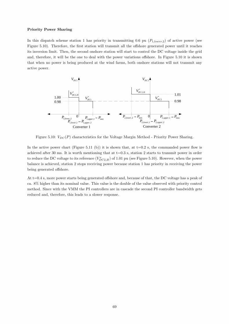
Priority Power Sharing
In this dispatch scheme station 1 has priority in transmitting 0.6 pu (P1,lower,2) of active power (see
Figure 5.10). Therefore, the first station will transmit all the offshore generated power until it reaches
its inversion limit. Then, the second onshore station will start to control the DC voltage inside the grid
and, therefore, it will be the one to deal with the power variations offshore. In Figure 5.10 it is shown
that when no power is being produced at the wind farms, both onshore stations will not transmit any
active power.
2DCV
0
Converter 2
2, ,1 maxupperP P2, ,2 minlowerP P
2, ,1 2, ,2lower upperP P
*
2,DC HV
*
2DCV
1DCV
0
1, ,1 1, ,2lower upperP P1, ,2lowerP
*
1DCV
*
1,DC HV
1, ,1 maxupperP P
Converter 1
0.98
1.000.98
1.01
Figure 5.10: VDC(P ) characteristics for the Voltage Margin Method - Priority Power Sharing.
In the active power chart (Figure 5.11 (b)) it is shown that, at t=0.2 s, the commanded power flow is
achieved after 30 ms. It is worth mentioning that at t=0.3 s, station 2 starts to transmit power in order
to reduce the DC voltage to its reference (V ∗DC2,H) of 1.01 pu (see Figure 5.10). However, when the power
balance is achieved, station 2 stops receiving power because station 1 has priority in receiving the power
being generated offshore.
At t=0.4 s, more power starts being generated offshore and, because of that, the DC voltage has a peak of
ca. 8% higher than its nominal value. This value is the double of the value observed with priority control
method. Since with the VMM the PI controllers are in cascade the second PI controller bandwidth gets
reduced and, therefore, this leads to a slower response.
69

0 0.1 0.2 0.3 0.4 0.5 0.6 0.7 0.8 0.9 10.97
0.98
0.99
1
1.01
1.02
1.03
1.04
1.05
1.06
1.07
1.08
time [s]
Vdc
[pu]
DC Voltage at the VSC stations
VSC 1VSC 2WF 1WF 2
0 0.1 0.2 0.3 0.4 0.5 0.6 0.7 0.8 0.9 1-1.2
-1
-0.8
-0.6
-0.4
-0.2
0
0.2
0.4
0.6
0.8
1
1.2
time [s]
Pdc
[pu]
Active Power at the VSC stations
VSC 1VSC 2WF 1WF 2
0 0.1 0.2 0.3 0.4 0.5 0.6 0.7 0.8 0.9 10.95
0.96
0.97
0.98
0.99
1
1.01
1.02
1.03
1.04
1.05
1.06
time [s]
|Vac
| [pu
]
AC Voltage at PCC
VSC 1VSC 2WF 1WF 2
0 0.1 0.2 0.3 0.4 0.5 0.6 0.7 0.8 0.9 1-0.15
-0.1
-0.05
0
0.05
0.1
0.15
time [s]
Qac
[pu]
Reactive Power at the VSC stations
VSC 1VSC 2WF 1WF 2
0 0.1 0.2 0.3 0.4 0.5 0.6 0.7 0.8 0.9 10.92
0.94
0.96
0.98
1
1.02
1.04
1.06
1.08
1.1
1.12
time [s]
|vc_
dq| [
pu]
Converter's AC Voltage
VSC 1VSC 2WF 1WF 2
0 0.1 0.2 0.3 0.4 0.5 0.6 0.7 0.8 0.9 1-0.1
0
0.1
0.2
0.3
0.4
0.5
0.6
0.7
0.8
0.9
1
1.1
time [s]
|ic_d
q| [p
u]
Converter's AC Current
VSC 1VSC 2WF 1WF 2
Figure 5.11: Simulation results using the Voltage Margin Method - Priority Power Sharing.
70
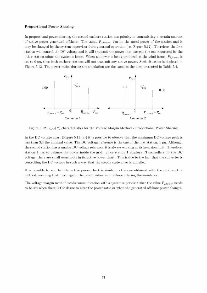
Proportional Power Sharing
In proportional power sharing, the second onshore station has priority in transmitting a certain amount
of active power generated offshore. The value, P2,lower, can be the rated power of the station and it
may be changed by the system supervisor during normal operation (see Figure 5.12). Therefore, the first
station will control the DC voltage and it will transmit the power that exceeds the one requested by the
other station minus the system’s losses. When no power is being produced at the wind farms, P2,lower is
set to 0 pu, thus both onshore stations will not transmit any active power. Such situation is depicted in
Figure 5.12. The power ratios during the simulation are the same as the ones presented in Table 5.4.
2DCV
02, ,1 maxupperP P
2, ,1lowerP
1DCV
01, ,1 maxupperP P
1, ,1 minlowerP P
Converter 1 Converter 2
*
1DCV *
2DCV1.000.98
Figure 5.12: VDC(P ) characteristics for the Voltage Margin Method - Proportional Power Sharing.
In the DC voltage chart (Figure 5.13 (a)) it is possible to observe that the maximum DC voltage peak is
less than 3% the nominal value. The DC voltage reference is the one of the first station, 1 pu. Although
the second station has a smaller DC voltage reference, it is always working at its inversion limit. Therefore,
station 1 has to balance the power inside the grid. Since station 1 employs PI controllers for the DC
voltage, there are small overshoots in its active power chart. This is due to the fact that the converter is
controlling the DC voltage in such a way that the steady state error is annulled.
It is possible to see that the active power chart is similar to the one obtained with the ratio control
method, meaning that, once again, the power ratios were followed during the simulation.
The voltage margin method needs communication with a system supervisor since the value P2,lower needs
to be set when there is the desire to alter the power ratio or when the generated offshore power changes.
71

0 0.1 0.2 0.3 0.4 0.5 0.6 0.7 0.8 0.9 10.97
0.98
0.99
1
1.01
1.02
1.03
1.04
1.05
1.06
1.07
1.08
time [s]
Vdc
[pu]
DC Voltage at the VSC stations
VSC 1VSC 2WF 1WF 2
0 0.1 0.2 0.3 0.4 0.5 0.6 0.7 0.8 0.9 1-1.2
-1
-0.8
-0.6
-0.4
-0.2
0
0.2
0.4
0.6
0.8
1
1.2
time [s]
Pdc
[pu]
Active Power at the VSC stations
VSC 1VSC 2WF 1WF 2
0 0.1 0.2 0.3 0.4 0.5 0.6 0.7 0.8 0.9 10.95
0.96
0.97
0.98
0.99
1
1.01
1.02
1.03
1.04
1.05
1.06
time [s]
|Vac
| [pu
]
AC Voltage at PCC
VSC 1VSC 2WF 1WF 2
0 0.1 0.2 0.3 0.4 0.5 0.6 0.7 0.8 0.9 1-0.15
-0.1
-0.05
0
0.05
0.1
0.15
time [s]
Qac
[pu]
Reactive Power at the VSC stations
VSC 1VSC 2WF 1WF 2
0 0.1 0.2 0.3 0.4 0.5 0.6 0.7 0.8 0.9 10.92
0.94
0.96
0.98
1
1.02
1.04
1.06
1.08
1.1
1.12
time [s]
|vc_
dq| [
pu]
Converter's AC Voltage
VSC 1VSC 2WF 1WF 2
0 0.1 0.2 0.3 0.4 0.5 0.6 0.7 0.8 0.9 1-0.1
0
0.1
0.2
0.3
0.4
0.5
0.6
0.7
0.8
0.9
1
1.1
time [s]
|ic_d
q| [p
u]
Converter's AC Current
VSC 1VSC 2WF 1WF 2
Figure 5.13: Simulation results using the Voltage Margin Method - Proportional Power Sharing.
72
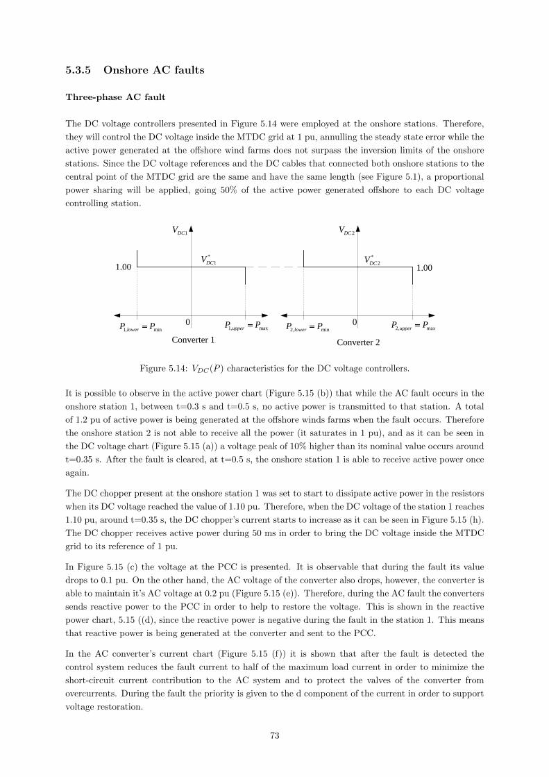
5.3.5 Onshore AC faults
Three-phase AC fault
The DC voltage controllers presented in Figure 5.14 were employed at the onshore stations. Therefore,
they will control the DC voltage inside the MTDC grid at 1 pu, annulling the steady state error while the
active power generated at the offshore wind farms does not surpass the inversion limits of the onshore
stations. Since the DC voltage references and the DC cables that connected both onshore stations to the
central point of the MTDC grid are the same and have the same length (see Figure 5.1), a proportional
power sharing will be applied, going 50% of the active power generated offshore to each DC voltage
controlling station.
1DCV
01, maxupperP P
1, minlowerP P
Converter 1 Converter 2
*
1DCV
2DCV
02, maxupperP P
2, minlowerP P
*
2DCV1.00 1.00
Figure 5.14: VDC(P ) characteristics for the DC voltage controllers.
It is possible to observe in the active power chart (Figure 5.15 (b)) that while the AC fault occurs in the
onshore station 1, between t=0.3 s and t=0.5 s, no active power is transmitted to that station. A total
of 1.2 pu of active power is being generated at the offshore winds farms when the fault occurs. Therefore
the onshore station 2 is not able to receive all the power (it saturates in 1 pu), and as it can be seen in
the DC voltage chart (Figure 5.15 (a)) a voltage peak of 10% higher than its nominal value occurs around
t=0.35 s. After the fault is cleared, at t=0.5 s, the onshore station 1 is able to receive active power once
again.
The DC chopper present at the onshore station 1 was set to start to dissipate active power in the resistors
when its DC voltage reached the value of 1.10 pu. Therefore, when the DC voltage of the station 1 reaches
1.10 pu, around t=0.35 s, the DC chopper’s current starts to increase as it can be seen in Figure 5.15 (h).
The DC chopper receives active power during 50 ms in order to bring the DC voltage inside the MTDC
grid to its reference of 1 pu.
In Figure 5.15 (c) the voltage at the PCC is presented. It is observable that during the fault its value
drops to 0.1 pu. On the other hand, the AC voltage of the converter also drops, however, the converter is
able to maintain it’s AC voltage at 0.2 pu (Figure 5.15 (e)). Therefore, during the AC fault the converters
sends reactive power to the PCC in order to help to restore the voltage. This is shown in the reactive
power chart, 5.15 ((d), since the reactive power is negative during the fault in the station 1. This means
that reactive power is being generated at the converter and sent to the PCC.
In the AC converter’s current chart (Figure 5.15 (f)) it is shown that after the fault is detected the
control system reduces the fault current to half of the maximum load current in order to minimize the
short-circuit current contribution to the AC system and to protect the valves of the converter from
overcurrents. During the fault the priority is given to the d component of the current in order to support
voltage restoration.
73
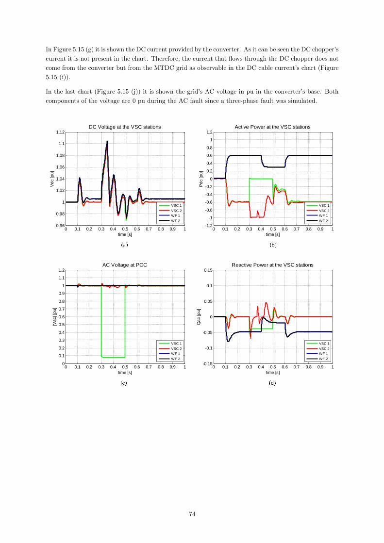
In Figure 5.15 (g) it is shown the DC current provided by the converter. As it can be seen the DC chopper’s
current it is not present in the chart. Therefore, the current that flows through the DC chopper does not
come from the converter but from the MTDC grid as observable in the DC cable current’s chart (Figure
5.15 (i)).
In the last chart (Figure 5.15 (j)) it is shown the grid’s AC voltage in pu in the converter’s base. Both
components of the voltage are 0 pu during the AC fault since a three-phase fault was simulated.
0 0.1 0.2 0.3 0.4 0.5 0.6 0.7 0.8 0.9 10.96
0.98
1
1.02
1.04
1.06
1.08
1.1
1.12
time [s]
Vdc
[pu]
DC Voltage at the VSC stations
VSC 1VSC 2WF 1WF 2
0 0.1 0.2 0.3 0.4 0.5 0.6 0.7 0.8 0.9 1-1.2
-1
-0.8
-0.6
-0.4
-0.2
0
0.2
0.4
0.6
0.8
1
1.2
time [s]
Pdc
[pu]
Active Power at the VSC stations
VSC 1VSC 2WF 1WF 2
0 0.1 0.2 0.3 0.4 0.5 0.6 0.7 0.8 0.9 1-0.15
-0.1
-0.05
0
0.05
0.1
0.15
time [s]
Qac
[pu]
Reactive Power at the VSC stations
VSC 1VSC 2WF 1WF 2
0 0.1 0.2 0.3 0.4 0.5 0.6 0.7 0.8 0.9 10
0.1
0.2
0.3
0.4
0.5
0.6
0.7
0.8
0.9
1
1.1
1.2
time [s]
|Vac
| [pu
]
AC Voltage at PCC
VSC 1VSC 2WF 1WF 2
74

0 0.1 0.2 0.3 0.4 0.5 0.6 0.7 0.8 0.9 1-0.1
0
0.1
0.2
0.3
0.4
0.5
0.6
0.7
0.8
0.9
1
1.1
time [s]
Idc
[pu]
Onshore station 1 - DC Current
VSC 1
0 0.1 0.2 0.3 0.4 0.5 0.6 0.7 0.8 0.9 1-0.1
0
0.1
0.2
0.3
0.4
0.5
0.6
0.7
0.8
0.9
1
1.1
time [s]
Icho
pper
[pu]
Onshore station 1 - DC Chopper's current
VSC 1
0 0.1 0.2 0.3 0.4 0.5 0.6 0.7 0.8 0.9 1-0.1
0
0.1
0.2
0.3
0.4
0.5
0.6
0.7
0.8
0.9
1
1.1
time [s]
Icab
le [p
u]
Onshore station 1 - DC cable's current
VSC 1
0 0.1 0.2 0.3 0.4 0.5 0.6 0.7 0.8 0.9 1-0.1
00.10.20.30.40.50.60.70.80.9
11.11.21.31.41.5
time [s]
Vgr
id [p
u]
Onshore station 1 - Grid's AC Voltage
d-axisq-axis
0 0.1 0.2 0.3 0.4 0.5 0.6 0.7 0.8 0.9 10
0.1
0.2
0.3
0.4
0.5
0.6
0.7
0.8
0.9
1
1.1
1.2
time [s]
|vc_
dq| [
pu]
Converter's AC Voltage
VSC 1VSC 2WF 1WF 2
0 0.1 0.2 0.3 0.4 0.5 0.6 0.7 0.8 0.9 1-0.1
0
0.1
0.2
0.3
0.4
0.5
0.6
0.7
0.8
0.9
1
1.1
time [s]
|ic_d
q| [p
u]
Converter's AC Current
VSC 1VSC 2WF 1WF 2
Figure 5.15: Simulation results of a onshore three-phase AC fault.
75

One-phase AC fault
The DC voltage controllers presented in Figure 5.14 were employed at the onshore stations.
In this simulation a one-phase AC fault was applied to the AC grid of the onshore station 1. Once again,
the fault started at t=0.3 s and it was cleared at t=0.5 s. The simulation results are shown in Figure
5.16.
In the active power chart (Figure 5.16 (b)) it is possible to see that, oppositely to what was observed in
the three-phase fault, the onshore station 1 does not stop receiving active power during the fault.
Important to refer that the charts of Figures 5.16 (c) and (e) show the average of the amplitude of the
voltages at the PCC and of the converter, respectively. As it is observable in Figure 5.16 (e), the voltage
at the PCC drops to approximately 0.7 pu. This result was expected since the system maintains two
healthy phases. In reality the voltage at the PCC is oscillatory. Therefore, the AC voltage of the converter
and the active and reactive powers are also oscillatory. This phenomenon occurs due to the fact that it
is not possible to achieve a synchronous rotative frame with the AC grid’s voltage since one the phases
is zero during the fault. However, the PCC and converter’s voltages do not drop as much as they did in
the three-phase AC fault simulation.
At t=0.5 s, after the fault’s clearance, the oscillatory response at the PCC voltage stops. Therefore, the
active and reactive power are no longer oscillatory.
Due to the fact that the onshore station 1 continues to receive active power during the fault, the DC
voltage inside the grid does not increase as much as it would be necessary to make the DC chopper to
start dissipating active power in the resistors.
Once again the control system, as soon as the fault is detected, set the converter’s current limit to
0.5 pu. Therefore, the converter valves are protected against overcurrents and the short-circuit current
contribution to the AC system is minimized. During the fault the priority is given to the d component
of the current in order to give priority to voltage restoration.
76
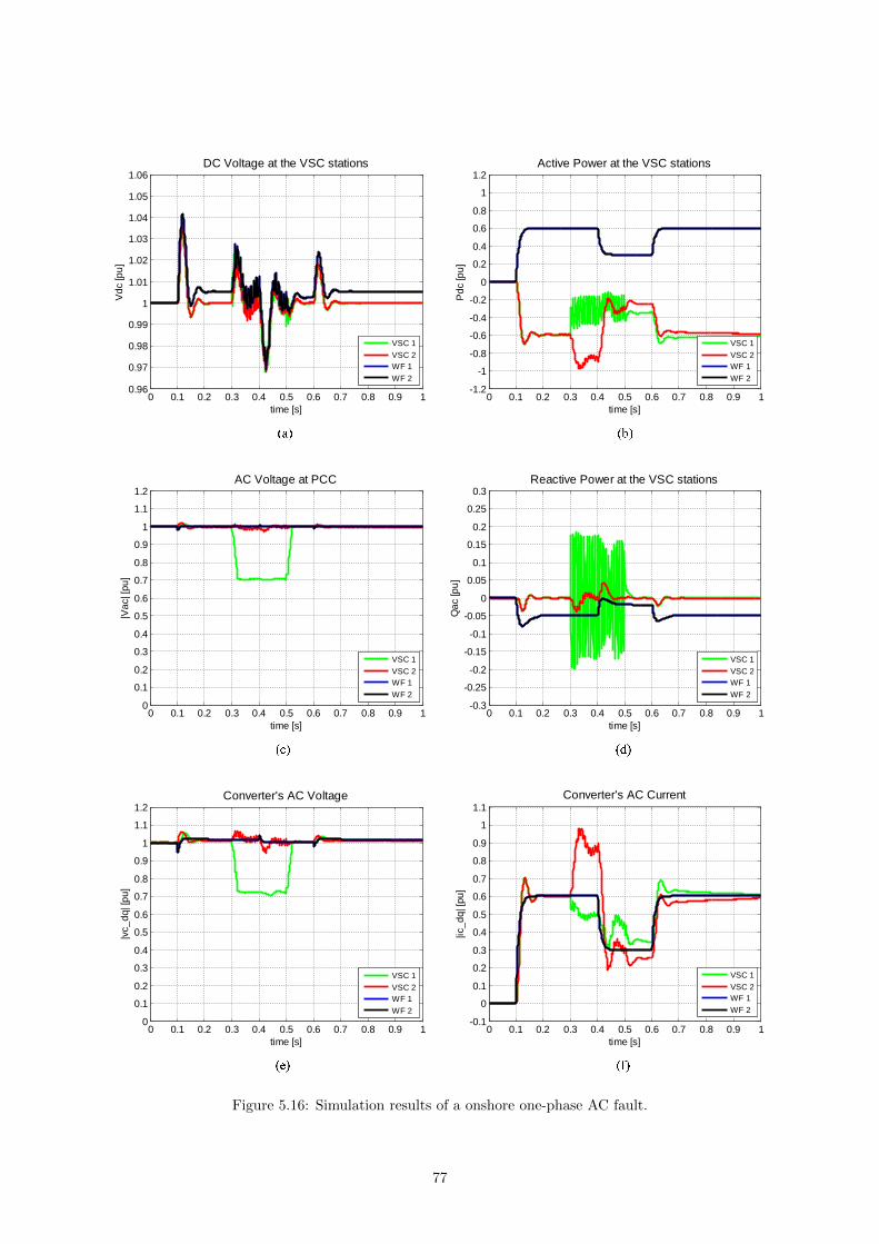
0 0.1 0.2 0.3 0.4 0.5 0.6 0.7 0.8 0.9 10.96
0.97
0.98
0.99
1
1.01
1.02
1.03
1.04
1.05
1.06
time [s]
Vdc
[pu]
DC Voltage at the VSC stations
VSC 1VSC 2WF 1WF 2
0 0.1 0.2 0.3 0.4 0.5 0.6 0.7 0.8 0.9 1-1.2
-1
-0.8
-0.6
-0.4
-0.2
0
0.2
0.4
0.6
0.8
1
1.2
time [s]
Pdc
[pu]
Active Power at the VSC stations
VSC 1VSC 2WF 1WF 2
0 0.1 0.2 0.3 0.4 0.5 0.6 0.7 0.8 0.9 1-0.3
-0.25
-0.2
-0.15
-0.1
-0.05
0
0.05
0.1
0.15
0.2
0.25
0.3
time [s]
Qac
[pu]
Reactive Power at the VSC stations
VSC 1VSC 2WF 1WF 2
0 0.1 0.2 0.3 0.4 0.5 0.6 0.7 0.8 0.9 1-0.1
0
0.1
0.2
0.3
0.4
0.5
0.6
0.7
0.8
0.9
1
1.1
time [s]
|ic_d
q| [p
u]
Converter's AC Current
VSC 1VSC 2WF 1WF 2
0 0.1 0.2 0.3 0.4 0.5 0.6 0.7 0.8 0.9 10
0.1
0.2
0.3
0.4
0.5
0.6
0.7
0.8
0.9
1
1.1
1.2
time [s]
|Vac
| [pu
]
AC Voltage at PCC
VSC 1VSC 2WF 1WF 2
0 0.1 0.2 0.3 0.4 0.5 0.6 0.7 0.8 0.9 10
0.1
0.2
0.3
0.4
0.5
0.6
0.7
0.8
0.9
1
1.1
1.2
time [s]
|vc_
dq| [
pu]
Converter's AC Voltage
VSC 1VSC 2WF 1WF 2
Figure 5.16: Simulation results of a onshore one-phase AC fault.
77

5.3.6 Offshore AC faults
Three-phase AC fault
The DC voltage controllers presented in Figure 5.14 were employed, once again, at the onshore stations
in this simulation.
A three-phase AC fault was applied to offshore wind farm 1. The simulation results are shown in Figure
5.17.
As it can be seen in the active power chart (Figure 5.17 (b)) the offshore wind farm 1 does not produce
any active power between t=0.3 s and t=0.5 s. However, when the three-phase is cleared at t=0.5 s, the
wind farm starts to transmit power once again to the MTDC grid.
A proportional power sharing of 50% was applied among the onshore stations during the simulation, thus
half of the active power being generated offshore is transmitted to each DC voltage controlling station.
In Figure 5.17 (c) the voltage at the PCC is presented. It is observable that during the fault it drops to
0.05 pu. On the other hand, the AC voltage of the converter also drops, however, the converter is able
to maintain it’s AC voltage around 0.2 pu. Therefore, during the AC fault the converters sends reactive
power to the PCC in order to help to restore the voltage. This can be seen in the reactive power chart
(Figure 5.17 (d)) since the reactive power is negative during the fault, meaning that reactive power is
being generated at the converter and sent to the PCC.
Once again, as soon as the fault is detected, the control system set the converter’s current limit to
0.5 pu. Therefore, the converter valves are protected against overcurrents and the short-circuit current
contribution to the wind farm is minimized. During the fault the priority is given to the d component of
the current in order to support voltage restoration.
78

0 0.1 0.2 0.3 0.4 0.5 0.6 0.7 0.8 0.9 10.96
0.97
0.98
0.99
1
1.01
1.02
1.03
1.04
1.05
1.06
time [s]
Vdc
[pu]
DC Voltage at the VSC stations
VSC 1VSC 2WF 1WF 2
0 0.1 0.2 0.3 0.4 0.5 0.6 0.7 0.8 0.9 1-1.2
-1
-0.8
-0.6
-0.4
-0.2
0
0.2
0.4
0.6
0.8
1
1.2
time [s]
Pdc
[pu]
Active Power at the VSC stations
VSC 1VSC 2WF 1WF 2
0 0.1 0.2 0.3 0.4 0.5 0.6 0.7 0.8 0.9 1-0.15
-0.1
-0.05
0
0.05
0.1
0.15
time [s]
Qac
[pu]
Reactive Power at the VSC stations
VSC 1VSC 2WF 1WF 2
0 0.1 0.2 0.3 0.4 0.5 0.6 0.7 0.8 0.9 1-0.1
0
0.1
0.2
0.3
0.4
0.5
0.6
0.7
0.8
0.9
1
1.1
time [s]
|ic_d
q| [p
u]
Converter's AC Current
VSC 1VSC 2WF 1WF 2
0 0.1 0.2 0.3 0.4 0.5 0.6 0.7 0.8 0.9 10
0.1
0.2
0.3
0.4
0.5
0.6
0.7
0.8
0.9
1
1.1
1.2
time [s]
|vc_
dq| [
pu]
Converter's AC Voltage
VSC 1VSC 2WF 1WF 2
0 0.1 0.2 0.3 0.4 0.5 0.6 0.7 0.8 0.9 10
0.1
0.2
0.3
0.4
0.5
0.6
0.7
0.8
0.9
1
1.1
1.2
time [s]
|Vac
| [pu
]
AC Voltage at PCC
VSC 1VSC 2WF 1WF 2
Figure 5.17: Simulation results of a offshore three-phase AC fault.
79

5.4 Comparison of the DC voltage control methods
In this section a comparison between the several DC voltage control methods implemented is presented.
In Table 5.5 the capability of the control method to perform the different dispatch schemes is shown.
It is important to refer that the Ratio Control is able to perform proportional power sharing without
communication if there are only two onshore DC voltage controlling stations connected to the MTDC grid.
However, as presented in Table 5.5, it is considered that the method actually requires communication.
Since future MTDC networks will most likely have more than two DC voltage controlling stations, the
method will require communication between them to share the total amount of offshore power being
produced at all times. On the other hand, the VMM requires communication to perform proportional
power sharing independently of the number of onshore stations.
Table 5.5: Capability of the DC voltage control methods to perform the dispatch schemes.
Onshore station 1st 2nd 1st 2nd 1st 2nd 1st 2nd
ControllersFixed Fixed Fixed Variable
PIFixed 2-stage 2-stage
Droop Droop Droop Droop Droop PI PIControl Method Droop Ratio Priority Voltage MarginFixed − − − +Priority + − + +Proportional − +* − +*
(+) - The DC voltage control method is able to perform the dispatch scheme.(−) - The DC voltage control method is not able to perform the dispatch scheme.(∗) - needs communication to perform that particular dispatch scheme.
In Table 5.6, the main characteristics of each method are presented. The methods are compared accord-
ingly to their dynamic response, expandability, flexibility, and the communication requirement.
The dynamic response reflects the speed with which the control method is able to minimize the transient
response of the DC voltage inside the MTDC grid with regard to the power variability from the onshore
wind farms. The expandability represents the possibility of controlling the DC voltage in MTDC grids
with a considerable number of nodes, while the flexibility characterizes the capability of each DC voltage
control strategy to perform the dispatch schemes. Finally, the communication requirement reflects the
need of each method for external data input to perform the dispatch schemes.
Table 5.6: Comparison of the different DC voltage control methods.
Control MethodDynamic
Expandability FlexibilityCommunication
Response Requirement
Droop High Medium Low LowRatio High Low Medium MediumPriority Medium Medium Medium LowVoltage Margin Low High High Medium
80
Chapter 6
Conclusions
Europe will benefit from the development of offshore wind power in many aspects. Firstly, the dependency
of the fossil fuel in the electricity production will decrease. Secondly, this offshore development will reduce
the CO2 emissions which meets the international engagements face to the climate changes.
The offshore development in the North Sea will include a DC interconnection between several countries.
Therefore, standardization is necessary to make it possible for early built DC transmissions to be part of
a future HVDC grid. For the offshore HVDC grid the types of HVDC converter and DC voltage must be
standardized.
This thesis presented a four terminal MTDC network linking two onshore grids and two offshore wind
farms through a radial DC grid. The main focuses were the development of a control system for the
stations, the creation of a model for the DC grid and the implementation of several strategies to control
the DC voltage of the stations that would allow the trade of energy accordingly different criteria between
the interconnected countries. The system was simulated in order to evaluate the model’s legitimacy and
accuracy. Simulink/MATLAB was the simulation tool employed.
When DC connections are concerned, two technologies are available: LCC-HVDC and VSC-HVDC. When
VSC technology is used, active power ratings are relatively lower when compared with those that are
possible to achieve with HVDC classic. This is the main reason why the latter is still preferred over the
first for bulk DC transmissions. On the other hand, VSC technology is suited for the offshore transmission
because of the smaller size of the converter which allows an easier and cheaper installation on an offshore
platform. Furthermore, this technology offers a significant advantage: the control of the active power
independently of the reactive power.
With the use of different modulation techniques the VSC can independently control the active power
flowing through the transmission system as well as the reactive power being exchanged with the connected
AC network. Therefore, different types of controllers and strategies can be used depending on the
environment chosen for the VSC-HVDC to operate. In this thesis, for the onshore stations the DC
voltage control was set for the active channel and the reactive power exchanged with the connected AC
network was the control chosen for the reactive channel. On the other hand, at the offshore stations, the
controls used were the active power generated at the wind farms for the active channel and the module
of the AC voltage at the PCC of the stations for the reactive channel.
The AC side of the VSC station was modeled as a controllable voltage source (where frequency, phase
angle and amplitude can be controlled independently) connected to an AC transmission network through
series reactors (transformer and phase reactor). On the other side, the DC part of the VSC link was
81
modeled as a controllable current source, controlled by instantaneous power balancing between the AC
and the DC side.
The VSC-HVDC control system structure was based on an inner current loop in combination with different
outer controllers. The purpose of the inner current controller is to guarantee that the AC current flowing
through the series reactance corresponds to the AC current reference without exceeding the converter
maximum current. The outer controllers are responsible for giving the inner current controller the AC
current reference values. The outer controllers include the already mentioned controls: reactive power
controller, the AC voltage controller, the active power controller, and the DC voltage controller.
The results of the simulations show that the system response is fast and the controls implemented accurate.
Active and reactive power can be controlled independently and flow bi-directionally: from the AC network
to the DC grid or the opposite.
The harmonic distortion caused by the switching of the converter valves has been neglected. This as-
sumption is possible since as explained in this thesis, the harmonic content of the VSC-HVDC voltages,
and therefore also of its currents, can be kept really low by the use of PWM techniques as well as AC
filters. Furthermore, the presence of series reactance between the station and the connected AC network
also contributes to the minimization of the harmonic distortion.
In this thesis several controllers for the DC voltage were implemented with the objective of studding their
performance and capability to perform several market dispatch schemes: fixed, priority, and proportional
power sharing.
The voltage droop control method is able to perform priority power sharing dispatch scheme. In order
to give priority to one of the onshore stations it is necessary to set the droop characteristic of the other
onshore station higher. Therefore, the priority station will transmit all the offshore generated power until
it reaches its limit. Then, the second onshore station starts to control the DC voltage inside the grid.
The extension of the voltage droop method to MTDC networks with more than two onshore stations
should be straightforward. The disadvantage of this control method as presented, is that it is not able
to perform fixed power sharing, i.e. the transmission of a constant power to a particular station in the
network is not possible.
Since the slope of the voltage droop characteristic is equivalent to a proportional control, the dynamic
behavior of the active power is given by the inner current controller loop, which has fast dynamics.
Therefore, the changes in the DC voltage occur almost instantaneously.
If the ratio control is employed, a static droop characteristic is set to one of the stations and a dynamic
one to the other onshore station. In the case study, the power ratio (n) between the onshore stations
varied during the simulation. The simulation results show that the power division is not exactly equal
to the value establish by the power ratio coefficient, however, the precision is high and above 95%. This
phenomenon is due to fact that the DC grid has losses. In addition, the analytic expression depends on
the resistance of the DC cables, which may vary, further affecting the method’s accuracy. It is possible
to perform the desired power ratio without the need for communication if one of the two onshore station
employs a fixed voltage droop characteristic. However, expandability is a downside of the ratio control
method since it is difficult to achieve an analytic expression for the power ratio when more than two DC
voltage control stations are connected to the DC grid.
In the priority control method the first onshore terminal will control the DC voltage at a reference value
until it reaches its rectification limit. The DC voltage steady-state error is null when the station that
employs a PI controller is in charge of controlling the grid voltage. When the first terminal saturates,
the second terminal starts receiving the exceeding power from the wind farms and the DC voltage varies
according to the droop characteristic of the second terminal. The priority control strategy is interesting
82

for small MTDC networks where a specific country wishes to have precedence over the power produced
by its wind farms and is willing to sell the exceeding power to neighbor countries connected to the DC
grid.
The last control strategy considered in this thesis was the voltage margin method. Among the methods
compared it is the one with highest flexibility since it is possible to implement all the dispatch schemes,
thus emulating the other DC voltage control strategies presented. The VMM is capable of performing
fixed power sharing and priority power sharing without depending on communication. However, in order
to perform proportional power sharing the control strategy requires communication with a supervisory
controller that will set the inversion limit of one of the onshore stations, accordingly.
While the other DC voltage control strategies have shown maximum DC voltage transients up to 4%
higher than the nominal voltage, for the VMM these transients were somehow higher, with the highest
overvoltage being of 8% higher than the nominal value in case of power imbalances inside the MTDC
grid. The reason for the worse transient response of the VMM could be because this method employs
cascaded PI controllers.
Although, the voltage droop control was dependent on the grid typology, the voltage margin method is
capable of performing DC voltage control interchangeably among the assigned converters and may work
without necessarily depending on the topology of the network [46].
Extending the voltage margin method to MTDC networks with a higher number of terminals should
be easier to accomplish than for the Ratio or Priority controllers. However, with a limited DC voltage
normal operating range, e.g. ±5% the nominal voltage, the maximum number of terminals that can be
controlled by the VMM may be limited to prevent adverse interaction between the controllers of each
terminal due to possible too low voltage margins.
In every DC voltage controller with a droop characteristic, margins were given between the minimum and
maximum values of the DC voltage to prevent the control gain from reaching excessive values. Otherwise,
the DC voltage can display an oscillatory or even have an unstable behavior.
It is important to notice that during the simulations, some of the generated active power is lost in the
DC cables due to their resistance. Thus, the power received onshore does not match the active power
generated offshore.
The most common and demanding AC fault scenarios, one-phase and three-phase faults, were also simu-
lated in order to test the capability of the VSC-HVDC model to maintain the link properly functioning
throughout the whole simulation time without disturbing the voltages on the non-faulted station and to
observe if the system returns to the previous steady-state condition shortly after the fault is solved.
Independently of the type of fault considered the VSC demonstrated its capability of recovering from the
fault, returning to the previous operating point shortly after the disturbance was cleared.
The DC choppers were installed in the DC voltage controlling stations since it is cheaper to install them
onshore. The DC chopper did not work for longer than 50 ms each time in order to avoid over-heating
the resistors.
Wind energy is a mature technology yet it is still increasing all over the world. As the onshore wind power
locations are becoming scarcer, countries are now starting to install offshore wind turbines, where space
is more abundant and the wind has higher speeds. The perspective of an offshore DC grid connecting
several countries in the North Sea has been in active consideration in the last years. Therefore, most
probably, a MTDC offshore grid will be built in the next decade.
83

Future work
Some aspects related with the VSC-HVDC technology that were not taken into consideration in this
thesis and could be subject for future work are:
• Implementation of a frequency control system. The frequency control is possible when the VSC is
connect to weak networks or passive loads, i.e. the VSC is the main source of power. The frequency
control in this case is obtained by varying the frequency of the valve pulse firing sequence in the
PWM technique;
• The standard 2- or 3-level VSC technology has no way of limiting DC fault currents due to the
presence of the free-wheeling diodes. Therefore, the presence of DC breakers in the model is needed
if DC faults are to be simulated;
• In order to perform proportional power sharing with more than two stations, the control strategy
requires a supervisor that sends information to the onshore stations. In this thesis, communication
delay was not considered. Therefore the capability of the control strategy to perform proportional
power sharing under a communication delay demands further exploration;
• Combination of the MTDC model with more realistic model of wind farms with different turbine
technologies;
• Test the capability of the MTDC on performing black-starts;
• The VSC capability chart was not implemented. However, its presence is very important since it
prevents the stations from working in overloaded operation points;
• In order to validate the control system developed in this thesis, an experimental setup should be
implemented.
84

Bibliography
[1] IEA, “World Energy Outlook,” Paris, 2010.
[2] EWEA, “Delivering Offshore Wind Power in Europe,” Bruxels, 2007.
[3] EWEA, “Wind Energy - The Facts,” Bruxels, 2009.
[4] A. A. van der Meer, R. Teixeira Pinto, and et al., “Offshore Transnational Grids in Europe: The
North Sea Transnational Grid Research Project in Relation to Other Research Initiatives,” presented
at the 9th International Workshop on Large-Scale Integration of Wind Power, Montreal, Que.,
Canada, October, 2010.
[5] J. Arrillaga, Y. Liu, and N. Watson, Flexible Power transmission - The HVDC Options. John Wiley
& Sons, Ltd, NYC, 2007.
[6] P. Bresesti, W. L. Kling, and et al., “Hvdc Connection of Offshore Wind Farms to the Transmission
System,” Energy Conversion, IEEE Transactions, vol. 22, pp. 37-43, 2007.
[7] N. M. Kirby, L. Xu, and et al., “HVDC Transmission for Large Offshore Wind Farms,” Power
Enginnering Journal, June, 2002.
[8] L. Livermore, D. J. Liang, and D. J. Ekanayake, “MTDC VSC Technology and its Applications for
Wind Power,” Universities Power Engineering Conference (UPEC), pp. 1-6 , August, 2010.
[9] EWEA, “Oceans of Opportunity,” Bruxels, 2009.
[10] M. Marques, “Steady State Analysis of the Interconnection of Offshore Energy Parks,” Master
Thesis, Instituto Superior Tecnico, Lisbon, 2010.
[11] “http://www.windatlas.dk/europe/oceanmap.html,” [online] Last accessed June 2011.
[12] ABB, “The abcs of HVDC Transmission Technology,” Sweden, 2007.
[13] M. Lemes, “HVDC Plus for Grid Access,” Brazil, 2010.
[14] T. Ackermann, Wind Power in Power Systems. John Wiley & Sons, Ltd, NYC, 2005.
[15] “http://www.principlepowerinc.com/products/windfloat.html,” [online] Last accessed June 2011.
[16] “www.treehugger.com/20090317-pelamis-wave-power.jpg,” [online] Last accessed June 2011.
[17] A. Estanqueiro and P. Costa, “Levantamento do potencial do paıs, limitacoes e solucoes tec-
nologicas,” in Energia Eolica Offshore, Lisbon, 2010.
[18] “www.energy.siemens.com/mx/pool/hq/power-transmission/hvdc/hvdc-
plus/converter/modularmultilevelconverter400.jpg,” [online] Last accessed September 2011.
85

[19] L. Zhang, Modeling and Control of VSC-HVDC Links Connected to Weak AC Systems. PhD Thesis,
Royal Institute of Technology, Stockholm, 2010.
[20] Airtricity, European supergrid, “http://www.trec-uk.org.uk/,” [online] Last accessed July 2011.
[21] R. Teixeira Pinto and P. Bauer, “The Role of Modularity Inside the North Sea Transnational Grid
Project: Modular Concepts for the Construction and Operation of Large Offshore Grids,” presented
at the Renewable Energy World Europe Conference, Milan, Italy, June, 2011.
[22] EWEA, “Wind in Power 2010 European Statistics,” Bruxels, 2011.
[23] K. Rudion, A. G. Orths, and et al., “First Steps in Developing a Future North-Sea Offshore Grid,”
presented at European Wind Energy Conference Exhibition, Warsaw, 2010.
[24] I. M. de Alegria, J. L. Martin, and et al., “Transmission Alternatives for Offshore Electrical Power,”
presented at Renewable and Sustainable Energy Reviews (2009), Volume: 13, Issue: 5, Pages: 1027-
1038, 2008.
[25] T. M. Haileselassie, M. Molinas, and T. Undeland, “Multi-terminal VSC-HVDC System for Integra-
tion of Offshore Wind Farms and Green Electrification of Platforms in the North Sea,” presented at
Nordic Workshop on Power and Industrial Electronics, June, 2008.
[26] K. Meah and S. Ula, “Comparative Evaluation of HVDC and HVAC Transmission Systems,” appears
in Power Engineering Society General Meeting, pp. 1-5, June, 2007.
[27] J. F. Chozas, H. C. Soerensen, and M. Korpas, “Integration of Wave and Offshore Wind Energy in
a European Offshore Grid,” Proceedings of the Twentieth (2010) International Offshore and Polar
Engineering Conference, Beijing, China, June, 2010.
[28] E. Spahic and G. Balzer, “Offshore Wind Farms - VSC-based HVDC Connection,” appears in Power
Tech, St. Petersburg, June, 2005.
[29] V. G. Agelidis, G. D. Demetriades, and N. Flourentzou, “Recent Advances in High-Voltage Direct-
Current Power Transmission Systems,” appears in Industrial Technology, Mumbai, December, 2006.
[30] S. Allebrod and et al., “New Transformerless, Scalable Modular multilevel Converters for HVDC-
Transmission,” appears in Power Electronics Specialists Conference, Rhodes, June, 2008.
[31] A. Lesnicar and R. Marquardt, “An Innovative Modular Multilevel Converter Topology Suitable for
a Wide Power Range,” presented at Power Tech Conference Proceedings, Germany, June, 2003.
[32] R. Teixeira Pinto, “Dynamics and Control of VSC-based HVDC Systems,” Master Thesis, Politecnico
di Torino, Torino, Italy, 2008.
[33] C. Du, VSC-HVDC for Industrial Power Systems. PhD Thesis, Chalmers University of Technology,
Sweden, 2007.
[34] C. Ismunandar, “Control of Multi-Terminal VSC-HVDC for Offshore Wind Power Integration,”
Master Thesis, Delft University of Technology, Delft, The Netherlands, 2010.
[35] T. Haileselassie, K. Uhlen, and T. Undeland, “Control of Multiterminal HVDC Transmission for
Offshore Wind Energy ,” presented at Nordic Wind Power Conference, Denmark, September, 2009.
[36] S. G. Johansson, G. Asplund, and et al., “Power System Stability Benefits with VSC DC-transmission
Systems,” CIGRE, Paris, 2004.
[37] A. Visioli, “Modified Anti-windup Scheme for PID Controllers,” appears in Control Theory and
Applications, Italy, January, 2003.
86
[38] A. Visioli, Advances in Industrial Control - Practical PID Control. Springer, 2006.
[39] O. Heyman, L. Weimers, and M.-L. Bohl, “HVDC - A Key Solution in Future Transmission Systems,”
Sweden, 2011.
[40] S. P. JL Thomas and A. Benchaib, “Analysis of a Robust DC-bus Voltage Control System for a VSC
Transmission Scheme,” presented at AC-DC Power Transmission, November, 2001.
[41] J. B. Stijn Cole and R. Belmans, “Generalized Dynamic VSC MTDC Model for power System
Stability Studies,” appears in Power Systems, IEEE Transactions, August, 2010.
[42] L. Xu, L. Yao, and M. Bazargan, “DC Grid Management of a Multi-terminal HVDC Transmission
System for Large Offshore Wind Farms,” presented at Sustainable Power Generation and Supply,
pp. 1-7, Nanjing , April, 2009.
[43] L. Xu, B. W. Williams, and L. Yao, “Multi-terminal DC Transmission Systems for Connecting Large
Offshore Wind Farms,” presented at Power and Energy Society General Meeting - Conversion and
Delivery of Electrical Energy in the 21st Century, Pittsburgh, July, 2008.
[44] B. Johnson and et al., “Expandable Multiterminal DC Systems based on Voltage Droop,” appears
in Power Delivery, IEEE Transactions, pp. 1926-1932, October, 1993.
[45] T. Nakajima and S. Irokawa, “A Control System for HVDC Transmission by Voltage Sourced Con-
verters,” presented at Power Engineering Society Summer Meeting, Edmonton, Canada, July, 1999.
[46] Y. Tokiwa and et al., “Novel Control Strategies for HVDC System with Self-contained Converter,”
appears in Electrical Engineering in Japan, pp. 19-26, 1993.
[47] S. K. Chaudhary and e. a. R. Teodorescu, “Chopper Controlled Resistors in VSC-HVDC Transmis-
sion for WPP with Full-scale Converters,” appears in Sustainable Alternative Energy (SAE), pp.
1-8, Valencia, Spain, September, 2009.
[48] C. Feltes, H. Wrede, and et, “Enhanced Fault Ride-Through Method for Wind Farms Connected to
the Grid Through VSC-based HVDC Transmission,” appears in Power Delivery, IEEE Transactions,
pp. 1537-1546, August, 2009.
[49] A. Arulampalam, G. Ramtharan, and et al., “Simulated Onshore-fault Ride Through of Offshore
Wind Farms Connected Through VSC HVDC,” appears in Wind Engineering, vol. 32, pp. 103-114,
2008.
[50] EWEA, “The European offshore Wind Industry - Key Trends and Statistics 2009,” Bruxels, 2010.
[51] ABB, “It’s Time to Connect With Offshore Wind Supplement,” Sweden, 2010.
[52] C. M. Dragan, “Multiterminal DC Connection for Offshore wind Farms,” Master Thesis, Aalborg
University, Denmark, 2009.
[53] L. P. Lazaridis, “Economic Comparison of HVAC and HVDC Solutions for large Offshore Wind
Farms under Special Consideration of Reliability,” Master Thesis, Royal Institute of Technology,
Stockholm, 2005.
[54] O. Martander, “DC Grids for Wind Farms,” Master Thesis, Chalmers University of Technology,
Sweden, 2002.
[55] N. B. Negra, J. Todorovic, and T. Ackermann, “Loss Evaluation of HVAC and HVDC Transmission
Solutions for Large Offshore Wind Farms,” 2005.
87

[56] EWEA, “Wind directions,” vol. 30, Bruxels, June, 2011.
[57] A. Sarmento, “Perspectivas e Metas da Energia Renovavel Oceanica em Portugal,” February, 2011.
[58] S. Cole, Steady-State and Dynamic Modelling of VSC HVDC Systems for Power System Simulation.
PhD Thesis, Katholieke Universiteit Leuven, Belgium, 2010.
[59] A. Orini and et al., “Trans Bay Cable - World’s First HVDC System using Multilevel Voltage-Sourced
Converter,” 2010.
[60] U. T. M. Mohan, Ned and W. P. Robbins, Power Electronics: Converters, Applications and Design.
2nd edition. John Wiley & Sons, Ltd, NYC, 1994.
[61] L. Harnefors, “Control of VSC-HVDC Transmissions,” Sweden, 2008.
[62] B. R. Andersen, “VSC Transmission - HVDC and Power Electronics,” presented at HVDC Collo-
quium, Oslo, Norway, April 2006.
[63] P. Kundur, Power System Stability and Control. McGraw-Hill, Inc, 1994.
[64] R. L. Hendriks, M. Gibescu, and et al., “Developing a Transnational Electricity Infrastructure Off-
shore: Interdependence between Technical and Regulatory Solutions,” appears in Power and Energy
Society General Meeting, pp. 1-6, July, 2010.
[65] E. Koldby and M. Hyttinen, “Challenges on the Road to an Offshore HVDC Grid,” presented in
Nordic Wind Power Conference, Bornholm, Denmark, September, 2009.
[66] M. Hyttinen, J. O. Lamell, and T. F. Nestli, “New Application of Voltage Source Converter (VSC)
HVDC to be Installed on the Gas Platform Troll A,” CIGRE, Paris, 2004.
[67] R. Teixeira Pinto, S. F. Rodrigues, P. Bauer, and J. Pierik, “Comparison of Direct Voltage Control
Methods of Multi-Terminal DC (MTDC) Networks through Modular Dynamic Models,” presented
at Power Electronics and Applications, pp. 1-10, Birmingham, United Kingdom , September, 2011.
[68] J. Liang and et al., “Control of Multi-Terminal VSC-HVDC Transmission for Offshore Wind Power,”
presented at Power Electronics and Applications, pp. 1-10, Barcelona, Spain, September, 2009.
[69] D. H. Saadat, “Basics of State Variable Modeling,” http://people.msoe.edu/, [online] Last accessed
June 2011.
88
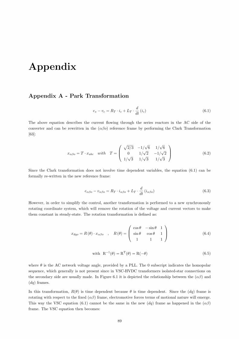
Appendix
Appendix A - Park Transformation
es − vc = RT · ic + LT ·d
dt(ic) (6.1)
The above equation describes the current flowing through the series reactors in the AC side of the
converter and can be rewritten in the (αβo) reference frame by performing the Clark Transformation
[63]:
xαβo = T · xabc with T =
√
2/3 −1/√
6 1/√
6
0 1/√
2 −1/√
2
1/√
3 1/√
3 1/√
3
(6.2)
Since the Clark transformation does not involve time dependent variables, the equation (6.1) can be
formally re-written in the new reference frame:
eαβo − vαβo = RT · iαβo + LT ·d
dt(iαβo) (6.3)
However, in order to simplify the control, another transformation is performed to a new synchronously
rotating coordinate system, which will remove the rotation of the voltage and current vectors to make
them constant in steady-state. The rotation transformation is defined as:
xdqo = R (θ) · xαβo , R (θ) =
cos θ − sin θ 1
sin θ cos θ 1
1 1 1
(6.4)
with R−1(θ) = RT(θ) = R(−θ) (6.5)
where θ is the AC network voltage angle, provided by a PLL. The 0 subscript indicates the homopolar
sequence, which generally is not present since in VSC-HVDC transformers isolated-star connections on
the secondary side are usually made. In Figure 6.1 it is depicted the relationship between the (αβ) and
(dq) frames.
In this transformation, R(θ) is time dependent because θ is time dependent. Since the (dq) frame is
rotating with respect to the fixed (αβ) frame, electromotive forces terms of motional nature will emerge.
This way the VSC equation (6.1) cannot be the same in the new (dq) frame as happened in the (αβ)
frame. The VSC equation then becomes:
89

d
q
x
x
x
qx dx
Figure 6.1: Relationship between the (αβ) and (dq) frames.
R (θ) eαβ −R (θ) vαβ = R (θ)RT · iαβ +R (θ)LT ·d
dt(iαβ)
⇔ edq − vdq = RT · idq +R (θ)LT ·d
dt
(R−1 (θ) · idq
) (6.6)
The difference between the VSC equation in the (dq) frame is the last term, which concerns the derivative
of the converter’s current. Evaluating this last term yields:
LT ·R (θ)
(d
dt
(R−1 (θ)
)· idq +R−1 (θ)
d
dt(idq)
)⇔ LT ·R (θ) · d
dt(R (−θ)) · idq + LT ·R (θ) ·R (−θ)︸ ︷︷ ︸
I
d
dt(idq)
⇔ LT ·
(cos θ − sin θ
sin θ cos θ
)· ddθ
[(cos θ sin θ
− sin θ cos θ
)]· ddt
(−θ)︸ ︷︷ ︸−ω
·idq + LT ·d
dt(idq)
⇔ LT ·
(0 1
−1 0
)︸ ︷︷ ︸
−j
· − ω · idq + LT ·d
dt(idq) = +jωLT · idq + LT ·
d
dt(idq)
(6.7)
Finally, the VSC equations, one for the d-axis and one for the q-axis, in the (dq) frame, to include the
new developed terms are:
ed − vd = RT · id + LT ·
d
dt(id)− ωLT · iq
eq − vq = RT · iq + LT ·d
dt(iq) + ωLT · id
(6.8)
90
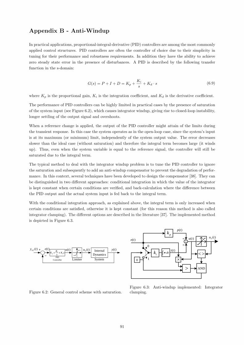
Appendix B - Anti-Windup
In practical applications, proportional-integral-derivative (PID) controllers are among the most commonly
applied control structures. PID controllers are often the controller of choice due to their simplicity in
tuning for their performance and robustness requirements. In addition they have the ability to achieve
zero steady state error in the presence of disturbances. A PID is described by the following transfer
function in the s-domain:
G(s) = P + I +D = Kp +Ki
s+Kd · s (6.9)
where Kp is the proportional gain, Ki is the integration coefficient, and Kd is the derivative coefficient.
The performance of PID controllers can be highly limited in practical cases by the presence of saturation
of the system input (see Figure 6.2), which causes integrator windup, giving rise to closed-loop instability,
longer settling of the output signal and overshoots.
When a reference change is applied, the output of the PID controller might attain of the limits during
the transient response. In this case the system operates as in the open-loop case, since the system’s input
is at its maximum (or minimum) limit, independently of the system output value. The error decreases
slower than the ideal case (without saturation) and therefore the integral term becomes large (it winds
up). Thus, even when the system variable is equal to the reference signal, the controller will still be
saturated due to the integral term.
The typical method to deal with the integrator windup problem is to tune the PID controller to ignore
the saturation and subsequently to add an anti-windup compensator to prevent the degradation of perfor-
mance. In this context, several techniques have been developed to design the compensator [38]. They can
be distinguished in two different approaches: conditional integration in which the value of the integrator
is kept constant when certain conditions are verified, and back-calculation where the difference between
the PID output and the actual system input is fed back to the integral term.
With the conditional integration approach, as explained above, the integral term is only increased when
certain conditions are satisfied, otherwise it is kept constant (for this reason this method is also called
integrator clamping). The different options are described in the literature [37]. The implemented method
is depicted in Figure 6.3.
Internal
Dynamics
( )e t ( )y t( )refy t
Limiter
( )u t ( )Su t
System
ip d
KK K s
sPID
Controller
Figure 6.2: General control scheme with saturation.
( )e t
( )p t
( )u t
( )i t
( )Su t
< >
AND>
×
ik dt
0
pk
0
1
Figure 6.3: Anti-windup implemented: Integratorclamping.
91
Appendix C - State-space model
The differential equations of a linear system can be written in the form:
x = Ax+Bu
y = Cx+Du(6.10)
This system of first-order differential equations is known as the state equation of the system, where x(t)
is the state vector and u(t) is the input vector. The second equation is referred to as the output equation.
A is called the state matrix, B the input matrix, C the output matrix and D the direct transition matrix.
One advantage of the state-space method is that the form lends itself easily to the digital and/or analog
computer methods of solution. Further, the state-space method can be easily extended for the analysis of
nonlinear systems. State equations may be obtained from an nth-order differential equation or directly
from the system model by identifying appropriate state variables [69].
To illustrate how is the selection of a set of state variables, an nth-order linear model described by a
differential equation is considered:
dny
dtn+ an−1
dn−1y
dtn−1+ · · ·+ a1
dy
dt+ a0y = u(t) (6.11)
where u(t) is the input and y(t) is the output. A state model for this system is not unique but depends
on the choice of a set of state variables. A useful set of state variables, referred to as phase variables, is
defined as:
x1 = y, x2 = y, x3 = y, · · · , xn = yn−1 (6.12)
Taking the derivatives, yields:
x1 = x2, x2 = x3, x3 = x4, · · · , xn = −a0x1 − a1x2 − · · · − an−1xn + u(t) (6.13)
or in matrix form:
x1
x2...
xn−1
xn
=
0 1 0 · · · 0
0 0 1 · · · 0...
......
......
0 0 0 · · · 1
−a0 −a1 −a2 · · · −an−1
x1
x2...
xn−1
xn
+
0
0
0...
1
u(t) (6.14)
The output equation is given by:
y =[
1 0 0 · · · 0]x (6.15)
For electrical networks, the state variables are directly related to the energy-storage elements of the
system. Therefore, the number of independent initial conditions is equal to the number of energy-storing
elements.
92