Embed Size (px)
Citation preview

Andy Sederman
Department of Chemical Engineering and Biotechnology, Cambridge
Dynamic MRI – Imaging Transport and
Structure in Transient Systems

The current team
Sponsors
Johnson Matthey, ExxonMobil, Shell, BP, Schlumberger,
AstraZeneca, GlaxoSmithKline, Merck Sharp & Dohme, NPL
Overview
• Introduction to MRI (and Chemical Engineering)
• Fast velocity imaging of fluids – dynamic flows
turbulent liquid flows
two phase flows
• chemical shift separation with compressed sensing
do we need an image?
• Bayesian analysis of acquired data
• Pharmaceutical dissolution testing
• Conclusions

What is Chemical Engineering? – and why use MR?
chemical process
technologypharmaceutical industryoil industry
many different chemical species
chemical reaction
fluid flows
porous media
optically opaque
The application of physical and life sciences to understand and develop
processes and products
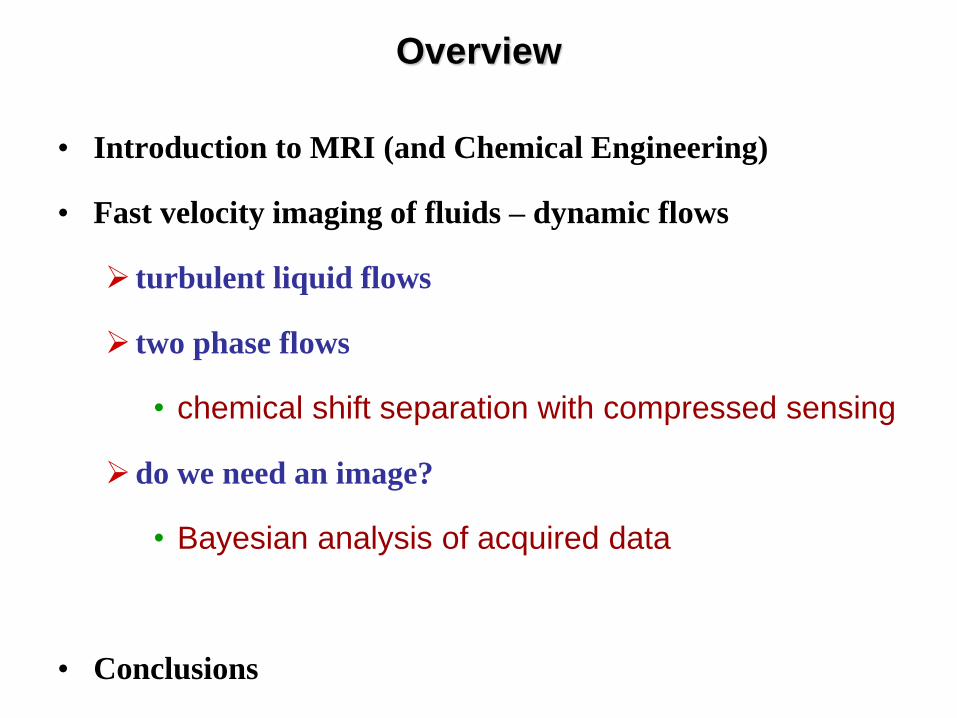
• Sample all of k and after FT we have a fully resolved image
k2
k-space raster
k1
image
FT
How to get a 2-D image with MRI: k-space
π2
γ tGk
rrkrk dS π2iexp)()(
krkkr dS π2iexp)()(
FT
rGr γ)(

Velocity imaging of flow in a pipe
• Steady flow up to Re ~ 2200
laminar Newtonian flow, parabolic velocity profile
• Onset of turbulence at higher Re
time varying flow
vdRe
0
10
20
30
40
50
60
70
-8 -4 0 4 8
ExperimentalAnalyticalV
elo
cit
y (
mm
s-1
)
Position (mm)
0.0 mm/s
10.0 mm/s
vz
y
x

Range of applicability
• Quantitative relationship between phase and displacement
measurement over wide range of velocities 10-6-102 m s-1
‘velocity’ over different timescales 10-3-101 s
Flow through single cell Flow over bluff body
van de Meent AJS, LFG et al.,
J. Fluid Mech, 642, 5 (2010)
MRI
Model
Newling et al., Phys. Rev.
Lett., 93(15), 154503 (2004)

• Many systems of practical interest demonstrate some
change with time
changing velocity
changing structure
• Imaging approaches to dynamic processes
time averaged
• image over long times compared to fluctuations
‘snapshot’ imaging
• speed up acquisitions
periodic systems
• triggered acquisitions
• How can MRI velocity imaging be used?
Dynamic processes

p/2 p p
d
D
Turbulent velocity imaging
ultra-fast velocity imaging sequence: GERVAIS
GERVAIS J Magn. Reson. 166 (2004) 182
Gradient Echo Rapid Velocity and Acceleration
Imaging Sequence
ky
k-space raster
kx
2D image time:
1 velocity component in 20 ms
3 velocity components in 60 ms

0 0
2vav 1.5vav
vz vzRe =1250
3300 4200 5000
1700 2500
x
y
z
Turbulent velocity imaging
Sederman et al., JMR, (2004)Pipe diameter: 29 mm, 1400 m × 700 m

Can we image even faster?
• We want to reduce timescales further
• 60 ms is still long for many systems
• Can we acquire all data points in a more efficient and
robust way?
faster images
minimise errors for high velocity flows
fast continuous image acquisition
• Do we need to acquire all of our k-space data points?
under-sampling – ‘sparse’ acquisition
non-FT reconstruction

Spiral imaging and compressed sensing
ky
k-space raster
kx

Spiral imaging and compressed sensing
r.f.
Gread 1
Gread 2
Gslice
Gvel
a
time
d
D
ky
k-space raster
kx
• Benefits
‘simple’ MRI pulse sequence
faster coverage of k-space – for given hardware limitations
robustness to velocity effects
short recycle ‘movie’ acquisition

Spiral imaging and compressed sensing
r.f.
Gread 1
Gread 2
Gslice
Gvel
a
time
d
D
ky
k-space raster
kx
• Benefits
‘simple’ MRI pulse sequence
faster coverage of k-space – for given hardware limitations
robustness to velocity effects
short recycle ‘movie’ acquisition

Spiral imaging and compressed sensing
r.f.
Gread 1
Gread 2
Gslice
Gvel
a
time
d
D
ky
k-space raster
kx
Andrew BlakeMicrosoft Research/Alan Turing Institute
• Compressed sensing
if an image can be represented in some transform
domain by significantly fewer data points, it must be
possible to acquire fewer data points in the first place

Spiral and CS: results
• High resolution pipe flow velocity images at Re = 5000
acquire 28% cf fully sampled image
64 × 64 pixels, resolution of 325 m × 325 m
repetition time of 5.3 ms, 188 fps
0z-
vel
oci
ty (
cm s
-1)
47

CS-Spiral velocity imaging of single bubbles
velocity images of water around a rising air
bubble
• single component velocity images in 5.3
ms
• 3-component velocity images in 16 ms
(63 fps)
• spatial resolution 390 m × 586 m
• field-of-view: 20 mm × 30 mm
• vortex shedding at a rate of 12.6 ± 1.1 Hz
• droplet rise velocity = 21 cm s-1
-15
y-v
elo
city
(cm
s-1
)
15
26.7 cm s-1in-plane (x-z) velocity:
25 m
m
x
z
y
Tayler Phys. Rev. Lett. (2012)

-8.9 26.9z-velocity (cm s-1)
in-plane velocity: 14.4 cm s-1
x
y
z
x
z
Why do bubbles wobble?
Phys. Rev. Lett. 108 (2012) 264505

direction of
bubble motion
direction
of wake
ab
y
x
0 200 400 600 800-p
0
p
p/2
p/2
a ,
b
time (ms)
b
a
-8.9 26.9z-velocity (cm s-1)
in-plane velocity: 14.4 cm s-1
x
y
z
x
z
Why do bubbles wobble?
• in addition to the counter-rotating vortices in longitudinal plane, there
exists a secondary mode of vorticity in the horizontal plane
•direct coupling between direction of bubble path and secondary
vortex; secondary vortices reverse direction following every
shedding event
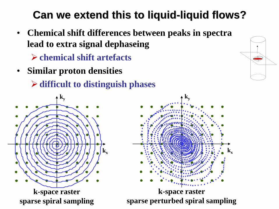
Can we extend this to liquid-liquid flows?
• Chemical shift differences between peaks in spectra
lead to extra signal dephaseing
chemical shift artefacts
• Similar proton densities
difficult to distinguish phases
ky
k-space raster
sparse spiral sampling
kx
ky
k-space raster
sparse perturbed spiral sampling
kx

Simultaneous measurement of oil and water flow fields50 cSt PDMS droplet rising through water
laboratory frame droplet framex
y
z
in-plane velocity7.2 cm s-1
droplet frame:
laboratory frame:
14.4 cm s-1
-14.4
14.4
z-velo
city (cm
s-1)
pipe diameter = 2 cm; droplet rise velocity = 7.1 cm s-1
data acquisition time = 31.8 ms
spatial resolution = 540 m 540 m; image slice thickness = 500 m
Tayler et al. Phys. Rev. E 89 (2014) 063009

Conventional
kx
ky
full sampling
Fourier
transform
Compressed
sensing
kx
sparse sampling
CS
reconstruction
increasing sparsity
faster acquisition
Why take an image? – A Bayesian approach

Conventional
kx
ky
full sampling
Fourier
transform
Bayesian
model +
Bayes’ theorem
kx
ky
selective sampling
pro
bab
ilit
y
size
increasing sparsity
faster acquisition
Compressed
sensing
kx
sparse sampling
CS
reconstruction
Why take an image? – A Bayesian approach

ky
kx
FT
10-10
10-9
10-8
10-7
10-6
-800 -400 0 400 800
sign
al
inte
nsi
ty (
a.u
.)
k (m-1
)
0
2 10-9
4 10-9
6 10-9
8 10-9
0 10 20 30 40
f(x)
x (mm)
10-10
10-9
10-8
10-7
10-6
-800 -400 0 400 800
sig
nal in
ten
sit
y (
a.u
.)
k (m-1
)
0
2 10-9
4 10-9
6 10-9
8 10-9
0 10 20 30 40
f(x)
x (mm)
FT
4 mm bubble16 mm bubble
Why take an image? – A Bayesian approach

0.0
0.2
0.4
0.6
0.8
1.0
1.2
0 1 2 3 4 5 6
pro
bab
ilit
y d
ensi
ty (
mm
-1)
diameter (mm)
optical
MR
Distribution I Distribution II
Bayesian bubble size measurement
0.0
0.2
0.4
0.6
0.8
1.0
1.2
0 1 2 3 4 5 6
pro
bab
ilit
y d
ensi
ty (
mm
-1)
diameter (mm)
Optical techniques cannot
be used at high voidage
Distribution III
0.0
0.2
0.4
0.6
0.8
1.0
1.2
0 1 2 3 4 5 6
pro
bab
ilit
y d
ensi
ty (
mm
-1)
diameter (mm)
optical
MR
comparison with optical measurements

Time resolved result
• Surfactants decrease the surface tension and, therefore, the bubble size
• Change in bubble size tracked in real time as a pulse of surfactant is
injected at the base of a bubble column
• Bubble size monitored every 3 s
air
pump
z
y water
overflow
0.0
0.2
0.4
0.6
0.8
0 200 400 600 800
rzrxsurfactant on?
voidage
r z,x (
mm
)
time (s)
0.0
0.1
0.2
0 200 400 600 800
void
age
time (s)
bubble size voidage
surfactant flow onsurfactant
solutionx
rx
rz
×
•

Summary
• MRI velocity imaging can be used to develop the
understanding of many dynamic processes
• More ‘intelligent’ data acquisition and reconstruction can
help to increase imaging speeds
image acquisition times as short as 5 ms
• Sometimes the important information can be obtained without
the need for an image
Bayesian analysis