Embed Size (px)
Citation preview

國 立 交 通 大 學
電子工程學系 電子研究所碩士班
碩 士 論 文
三模MIMO之無線區域網路
等化器設計
A Tri-mode MIMO Equalizer Design for OFDM Based Wireless LANs
研 究 生:黃俊彥 Jun-Yen Huang
指導教授:溫瓌岸 博士 Dr. Kuei-Ann Wen
中 華 民 國 九 十 七 年 六 月
三模MIMO之無線區域網路
等化器設計
A Tri-mode MIMO Equalizer Design
for OFDM Based Wireless LANs
研 究 生:黃俊彥 Student : Jun-Yen Huang
指導教授:溫瓌岸 博士 Advisor : Dr. Kuei-Ann Wen
國 立 交 通 大 學
電子工程學系 電子研究所碩士班
碩 士 論 文
A Thesis
Submitted to Department of Electronics Engineering & Institute of
Electronics
College of Electrical & Computer Engineering
National Chiao Tung University
in Partial Fulfillment of the Requirements
for the Degree of Master
in
Electronic Engineering
June 2008
中 華 民 國 九 十 七 年 六 月

i
三模MIMO之無線區域網路
等化器設計
研究生:黃俊彥 指導教授: 溫瓌岸博士
國立交通大學
電子工程學系 電子研究所碩士班
摘要 本論文提出一個可操作在具兩個傳送天線與兩個接收天線的三模等化器
(Equalizer)。所提出的三模等化器,在高速的無線區域網路(Wireless LANs)中,
可操作模式包含 SISO模式、SDM-MIMO模式和 STBC-MIMO模式共三個模式。
為考慮載波頻率偏移(Carrier Frequency Offset, CFO) 對系統的影響,本論文提出
一個方法來有效率的減緩剩餘載波頻率偏移(Residual CFO)所造成的影響,以降
低通道估測的錯誤。接著,提出一個高效率的載波頻率偏移追蹤器可以有效的降
低系統封包錯誤率(Packet Error Rate)。
模擬結果顯示使用上述的方法可以在 2x2 多重輸入多重輸出(Multi-Input
Multi-Output)的系統中,將剩餘載波頻率偏移對封包錯誤率的影響減低至 0.2dB
以內。考慮到實際的硬體實現,先觀察在三個模式中所使用演算法的相似度,在
所提出的三模等化器架構中大量使用共用架構來減少面積消耗。最後,我們使用
FPGA來實現所提出的電路。

ii
A Tri-mode MIMO Equalizer Design for OFDM Based Wireless LANs
Student: Jun-Yen Huang Advisor: Dr. Kuei-Ann Wen
Department of Electronics Engineering Institute of Electronics
National Chiao-Tung University
Abstract In this thesis, an efficient hardware architecture for tri-mode equalizer with two
transmit and two receive antennas is proposed. The proposed tri-mode equalizer
supports SISO, SDM-MIMO and STBC-MIMO for wireless LANs is designed.
Considering the effects of carrier frequency offset (CFO), an effective CFO mitigation
method is proposed to reduce the channel estimation error caused by residual CFO.
Then, an effective CFO tracking algorithm is also proposed to enhance packet error
rate (PER) performance.
Simulation results show that the proposed CFO mitigation and tracking
algorithm can effectively suppress the PER performance loss due to residual CFO
within 0.2 dB in the 2x2 multi-input multi-output (MIMO) system. For practical
implementation, a lot of shared-architectures are utilized to reduce area consumption
of the tri-mode equalizer by observing the similarity in the algorithms of the three
modes. FPGA is used to implement our design.

iii
誌 謝
首先,第一個要感謝的是指導教授,溫瓌岸教授。感謝老師在兩年研究生
涯中,不斷的給予俊彥指導與督促。溫老師的循循教誨,讓學生在學習訓練的路
途上,能夠快速而正確的修正自己的研究方向,並且保持不鬆懈的心態進行研
究。也感謝 TWT_LAB 在這兩年中提供的豐富研究資源,讓我在研究上無後顧之
憂。另外,感謝各位口試委員們─李鎮宜教授與王晉良教授百忙中撥空提供寶貴
的建議與指教,使得本論文更加的完整。
感謝實驗室的學長姐們的指導與照顧:嘉笙學長、文燊學長、哲生學長、
文安學長、晧名學長、立協學長、懷仁學長、彥凱學長、建毓學長、翔琮學長及
凱信學長等在研究上的意見與幫助。
感謝實驗室的同學們-柏麟、謙若、士賢、磊中、佳欣、國爵,二年來在課
業和日常生活上總是相互的扶持與幫助。因為有你們,在趕進度的日子裡也能充
滿歡笑,遇到困難時,大家都互相幫忙解決問題。同時也要感謝實驗室的助理們:
苑佳、淑怡、慶宏、恩齊、智伶、嘉誠、宛君,幫忙實驗室裡大大小小的事,讓
我們能更專心於研究。
最後,感謝默默支持我的家人及朋友。有你們的支持與分憂解勞,讓我可以
無後顧之憂,全心的完成學業與研究,在此致上最深的感謝。
黃俊彥
2008
iv
Contents
摘要............................................................................................................................i
Abstract .................................................................................................................... ii
誌 謝 ................................................................................................................. iii
Contents....................................................................................................................iv
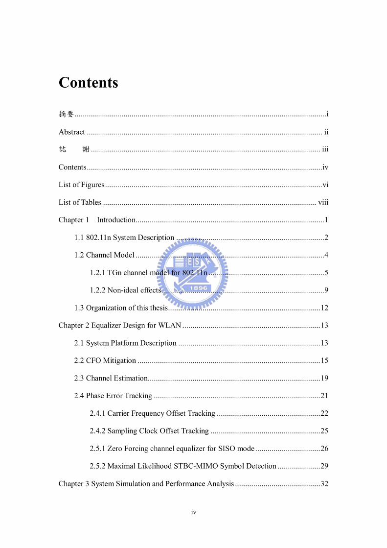
List of Figures...........................................................................................................vi
List of Tables ......................................................................................................... viii
Chapter 1 Introduction.............................................................................................1
1.1 802.11n System Description .........................................................................2
1.2 Channel Model .............................................................................................4
1.2.1 TGn channel model for 802.11n .........................................................5
1.2.2 Non-ideal effects................................................................................9
1.3 Organization of this thesis...........................................................................12
Chapter 2 Equalizer Design for WLAN ....................................................................13
2.1 System Platform Description ......................................................................13
2.2 CFO Mitigation ..........................................................................................15
2.3 Channel Estimation.....................................................................................19
2.4 Phase Error Tracking ..................................................................................21
2.4.1 Carrier Frequency Offset Tracking ...................................................22
2.4.2 Sampling Clock Offset Tracking ......................................................25
2.5.1 Zero Forcing channel equalizer for SISO mode ................................26
2.5.2 Maximal Likelihood STBC-MIMO Symbol Detection .....................29
Chapter 3 System Simulation and Performance Analysis ..........................................32

v
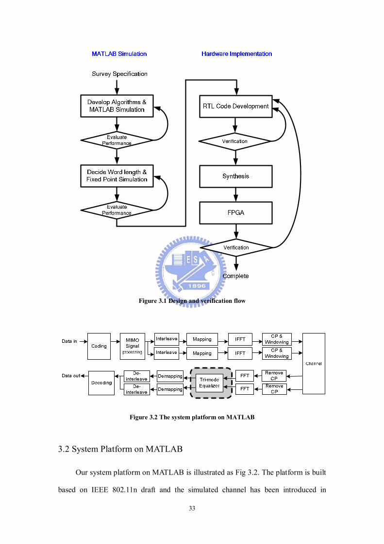
3.1 Design and Verification Flow......................................................................32
3.2 System Platform on MATLAB....................................................................33
3.3 Performance Analysis .................................................................................34
3.3.1 Channel Estimation Accuracy Analysis ............................................35
3.3.2 Phase Error Tracking Performance Analysis .....................................36
3.3.3 System Performance ........................................................................37
Chapter 4 Hardware Implementation ........................................................................40
4.1 Common Architecture Design for Tri-mode Equalizer ................................40
4.2 Modules Design..........................................................................................41
4.2.1 CFO Mitigation Module Design .......................................................41
4.2.2 Channel Estimation Module Design .................................................42
4.2.3 Phase Error Tracking Module Design...............................................43
4.2.4 MIMO Detection Module Design.....................................................45
4.2.5 CORDIC Module Design .................................................................47
4.3 Implementation Results ..............................................................................49
4.3.1 Fixed-point Simulation.....................................................................49
4.3.2 Hardware Synthesis..........................................................................51
Chapter 5 Conclusions and Future Works .................................................................55
Bibliography ............................................................................................................57
Vita ..........................................................................................................................60
vi
List of Figures
Figure 1.1: 802.11a/g and 802.11n preamble format............................................... 3
Figure 1.2: Baseband channel model...................................................................... 5
Figure 1.3: TGn channel model D delay profile ..................................................... 6
Figure 1.4: AOA (or AOD) of a Laplacian distribution, AS = 30o........................... 7
Figure 1.5: Carrier frequency offset effect.............................................................. 10
Figure 1.6: Mismatches between ADC/DAC sample frequencies ........................... 11
Figure 2.1: System block diagram.......................................................................... 14
Figure 2.2: MIMO signal processing...................................................................... 14
Figure 2.3: Training symbols of 802.11n................................................................ 15
Figure 2.4: The principle of D-symbol estimation .................................................. 16
Figure 2.5: Training symbols required for proposed CFO mitigation...................... 18
Figure 2.6: Smooth the estimated channels with a 3 taps fir filter ........................... 20
Figure 2.7: 2x2 MIMO Channel Estimation for 802.11n ........................................ 20
Figure 2.8: 64QAM data constellation: (a) without PET (b) with PET.................... 22
Figure 2.9: Constellation diagram of MMSE detection under different SNR .......... 29
Figure 2.10: Constellation diagram of ML detection under different SNR................ 31
Figure 3.1: Design and verification flow ................................................................ 33
Figure 3.2: The system platform on MATLAB....................................................... 33
Figure 3.3: Mean channel estimation errors vs. SNR under different CFO mitigation
algorithms............................................................................................ 35
Figure 3.4: Compare PET Algorithms at 2x2 MIMO, QPSK, ½ Code rate ............. 36
Figure 3.5: PER performance on STBC mode........................................................ 38
Figure 4.1: Tri-mode equalizer architecture............................................................ 40
Figure 4.2: The proposed CFO mitigation architecture........................................... 41
Figure 4.3: Tri-mode architecture of channel estimator .......................................... 42

vii
Figure 4.4: The proposed Tri-mode CFO tracker architecture................................. 44
Figure 4.5: Tri-mode MIMO Detector architecture................................................. 46
Figure 4.6: The architecture of CORDIC cell at i-th stage ...................................... 48
Figure 4.7: The architecture of CORDIC module ................................................... 48
Figure 4.8: The normalized angle........................................................................... 49
Figure 4.9: Performance comparisons between floating point and fixed point
simulation ............................................................................................ 50
Figure 4.10: The synthesis report of tri-mode equalizer on ISE ................................ 53
Figure 4.11: Comparison of RTL simulation and FPGA emulation........................... 53
Figure 4.12: VeriComm and FPGA board................................................................. 54
viii
List of Tables
Table 1.1: Physical layer related parameters ......................................................... 1
Table 1.2: TGn channel model parameters............................................................ 5
Table 1.3: TGn channel model D parameters ........................................................ 8
Table 2.1: Transmitted signals for 2x2 STBC-MIMO ........................................... 30
Table 3.1: PER Performance Comparison on SISO/SDM ..................................... 37
Table 3.2: System constraint for 802.11a and the required SNR to meet 10% PER
for STBC-MIMO for 802.11n .............................................................. 39
Table 4.1: Bit numbers of main modules............................................................... 50
Table 4.2: Hardware complexity of the tri-mode equalizer.................................... 51
Table 4.3: Gate count comparison for 2x2 MIMO symbol detectors ..................... 51

1
Chapter 1 Introduction
Higher and higher data rates transmission are demanded for various multimedia
applications in the wireless network. To increase the data rate and the robustness of
transmission, the MIMO-OFDM technologies are first introduced in 802.11n wireless
LAN system for various applications. IEEE 802.11n is developed based on IEEE
802.11a/g. The highest data rate can be outstandingly raised from 54Mbps to
600Mbps by using the additional antennas. The comparison of the physical layer
related parameters are listed in Table 1.1. The differences between 802.11a/g and
802.11n include increasing the number of data sub-carriers, adding the optional
40MHz bandwidth operation, adding the 5/6 coding rate, and the optional half guard
interval. All these adjustments are used to raise the maximum data transmission
throughput.
Table 1.1 Physical layer related parameters
MIMO-OFDMSISO-OFDMTechnology
20MHz/40MHz20MHzBandwidth
1/2 2/3 3/4 5/61/2 2/3 3/4 Coding rate
4μsec4μsecSymbol interval
312.5kHz312.5kHzSubcarrier spacing
600Mbps54MbpsMax data rate
56/114(52/108 data subcarriers)
52(48 data subcarriers)
Total number of subcarriers
64/12864FFT size
802.11n802.11a/g
MIMO-OFDMSISO-OFDMTechnology
20MHz/40MHz20MHzBandwidth
1/2 2/3 3/4 5/61/2 2/3 3/4 Coding rate
4μsec4μsecSymbol interval
312.5kHz312.5kHzSubcarrier spacing
600Mbps54MbpsMax data rate
56/114(52/108 data subcarriers)
52(48 data subcarriers)
Total number of subcarriers
64/12864FFT size
802.11n802.11a/g

2
The distinct feature in baseband is the use of MIMO-OFDM technology. MIMO
techniques can basically be classified into two groups: space division multiplexing
(SDM) and space time coding (STC). SDM achieves a higher throughput by
transmitting independent data streams on the different transmit branches
simultaneously and at the same carrier frequency. On the other hand, STC increases
the performance of the communication system by coding over the different transmitter
branches. Space time block coding (STBC) is the STC technique indicated in 802.11n.
STBC is first introduced by Alamouti [1], and is extended by Tarokh [2]. It has a
main advantage of low complexity in hardware implementation.
Orthogonal frequency division multiplexing (OFDM) has been selected as the
basis for several standards recently due to its advantages of dealing with multi-path
outstandingly, reducing the complexity of equalizer, making single frequency possible,
and high spectral efficiency. Further, Combining MIMO and OFDM technologies,
MIMO-OFDM systems benefit from high throughput and high performance
promising the future potential of the wireless networks.
1.1 802.11n System Description
In 802.11n, SDM-MIMO achieving high spectral efficiency is mandatory.
STBC-MIMO which increases system performance is an optional robust transmission.
Legacy SISO mode increasing the flexibility of usage are also supported by 802.11n.
Conventionally, three different equalizers are used to decode the data from the three
different modes, respectively. To utilize resources effectively and provide more
flexibility of usage, a tri-mode equalizer supporting SISO, 2x2 SDM-MIMO and 2x2
STBC-MIMO for 802.11n applications is the design target.

3
Figure 1.1 802.11a/g and 802.11n preamble format
The preamble in mixed-mode for 802.11n can be divided to two portions. In
addition to new defined high-throughput portion, it concatenates the legacy preamble
structure for 802.11a/g, i.e. compatibility portion. The reason is that the compatibility
portion can be recognized by 802.11a/g systems, so this structure has the advantage of
backward compatibility, and thus the flexibility of usage increases. We can realize the
preamble structure clearly from Fig 1.1.
Similar to OFDM systems, MIMO-OFDM systems are very sensitive to phase
errors. Even carrier frequency offset (CFO) estimation error (or residual CFO) shifts
the sub-carrier frequencies and consequently introduces severe phase errors in OFDM.
In addition, the accuracy of the channel estimation is also degraded by residual CFO,
causing PER performance loss of the receiver. Accurate channel estimation is
required to prevent inter-spatial stream interference (ISSI) in MIMO system
particularly. Therefore, residual CFO must be estimated and compensated to ensure
reliable communication with MIMO-OFDM.
With the repeated structure at legacy short training field (L-STF),
autocorrelation-based techniques [3] at time domain are commonly used to estimate
coarse CFO for practical implementation at receiver. The estimation errors left by
coarse CFO estimation still cannot be neglected for system performance. In general,

4
with the repeated long preambles structure, i.e. L-LTF, an autocorrelation-based
estimation [3] in time domain is utilized again for fine CFO estimation to determine
the residue of the coarse CFO correction. After coarse and fine CFO estimation, we
can get a satisfied performance in SISO mode for CFO reduction.
However, the channel estimation accuracy degraded by residual CFO for MIMO
modes is still severe in 802.11n mixed-mode due to the large time lag between the
L-LTF and the HT-LTFs which are used to estimate the MIMO channels [4]. Besides,
while tracking the phase errors caused by CFO and SCO in the data potion, the
existing pilot-based phase error tracking (PET) algorithms can not get a good
performance against residual CFO due to few pilot numbers in wireless LANs.
In this study, a simple CFO mitigation method is proposed to help reduce the
channel estimation error for mixed-mode in 802.11n by exploiting the structure of the
packet preamble. Then an effective phase error tracking algorithm is also proposed to
totally solve the CFO issues. We will demonstrate that with the proposed techniques,
there is little loss due to CFO in system performance.
1.2 Channel Model
In this section, the channel model used for system simulation is introduced. In
addition to the TGn proposed MIMO channel models [5], some non-ideal effects at
receiver are added according to the TGn comparison criteria [6]. Non-ideal effects at
receiver include additive white Gaussian noise (AWGN), CFO, and sampling clock
offset (SCO). The baseband channel model used for simulation is illustrated as Fig 1.2.
The TGn proposed channel models will be described in 1.2.1; the non-ideal effects
will be introduced in 1.2.2.

5
TX1
TX2
RX1
RX2
TGnChannelModel
AWGN
2jNeεπ δ
CFO SCO
NoiseBaseband
Channel Model
1.2.1 TGn channel model for 802.11n
TGn classifies the indoor channel environments to six types and six models A-F
are used to simulate the different channel conditions respectively. The sizes of
environments increase from A to F. The parameters of channel models are listed in
Table 1.2.
Table 1.2 TGn channel model parameters
186150F
184100E
18350D
14230C
9215B
110A
Number of taps
Number of clusters
RMS delay spread (ns)
Channel Model
186150F
184100E
18350D
14230C
9215B
110A
Number of taps
Number of clusters
RMS delay spread (ns)
Channel Model
In the following, we briefly introduce the channel related parameters, and then
explain how to develop MIMO channels.
Figure 1.2 Baseband channel model.
6
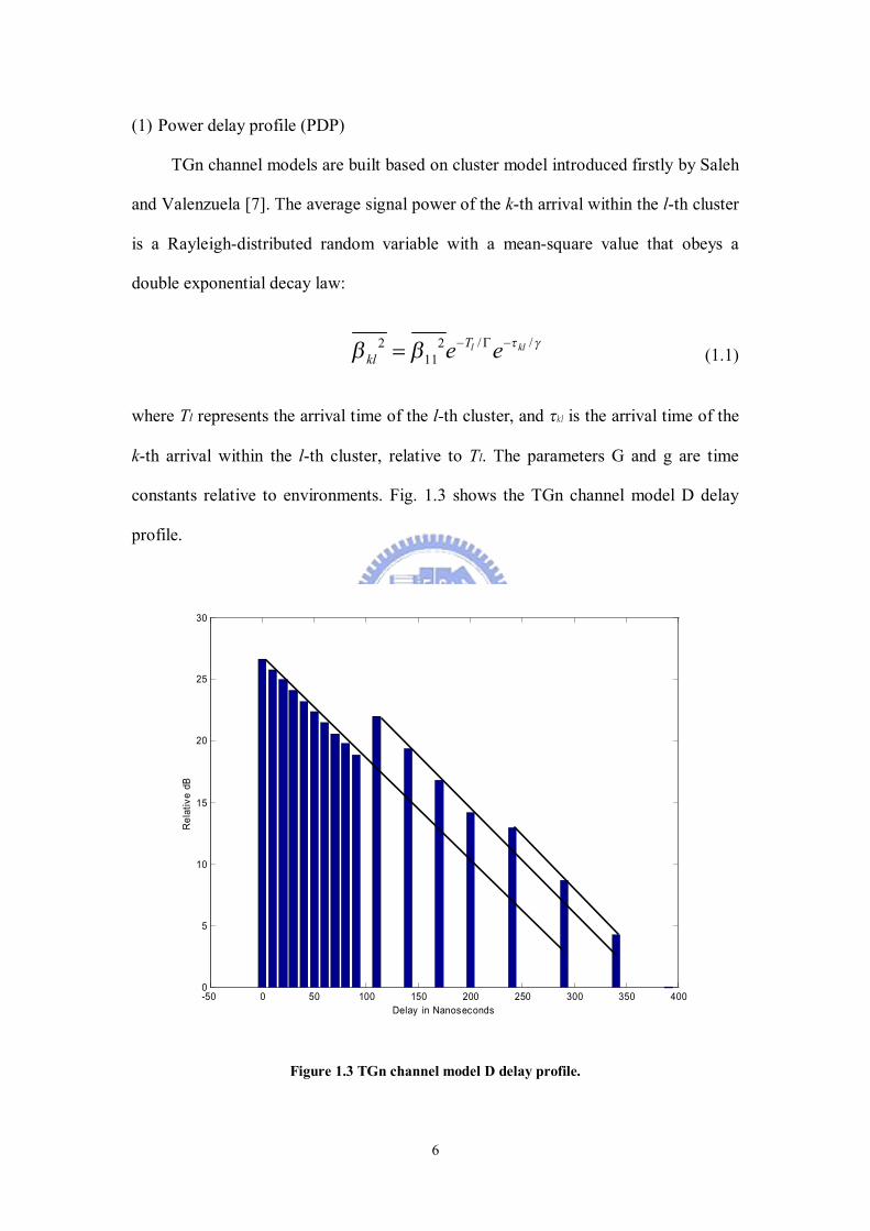
(1) Power delay profile (PDP)
TGn channel models are built based on cluster model introduced firstly by Saleh
and Valenzuela [7]. The average signal power of the k-th arrival within the l-th cluster
is a Rayleigh-distributed random variable with a mean-square value that obeys a
double exponential decay law:
/ /2 211
l klTkl e e τ γβ β − Γ −= (1.1)
where Tl represents the arrival time of the l-th cluster, and τkl is the arrival time of the
k-th arrival within the l-th cluster, relative to Tl. The parameters G and g are time
constants relative to environments. Fig. 1.3 shows the TGn channel model D delay
profile.
Figure 1.3 TGn channel model D delay profile.
-50 0 50 100 150 200 250 300 350 4000
5
10
15
20
25
30
Delay in Nanoseconds
Rel
ativ
e dB

7
(2) Power Angular Spread (PAS)
The angle of arrival statistics within a cluster were found to closely match the
Laplacian distribution [8-10]
2 /1( )2
p e θ σθσ
−= (1.2)
where σ is the standard deviation of the PAS (which corresponds to the numerical
value of angular spread; AS). The Laplacian distribution is shown in Fig 1.4 (a typical
simulated distribution within a cluster, with AS = 30o).
Finally, the parameters of channel model D which is a typical office
environment are listed in Table 1.3.
Figure 1.4 AOA (or AOD) of a Laplacian distribution, AS = 30o.

8
Table 1.3 TGn channel model D parameters.
Tap index 1 2 3 4 5 6 7 8 9 10 11 12 13 14 15 16 17 18
Excess delay [ns]
0 10 20 30 40 50 60 70 80 90 110 140 170 200 240 290 340 390
Cluster 1 Power [dB] 0 -0.9 -1.7 -2.6 -3.5 -4.3 -5.2 -6.1 -6.9 -7.8 -9.0 -11.1 -13.7 -16.3 -19.3 -23.2
AoA
AoA [°] 158.9 158.9 158.9 158.9 158.9 158.9 158.9 158.9 158.9 158.9 158.9 158.9 158.9 158.9 158.9 158.9
AS (RX)
AS [°] 27.7 27.7 27.7 27.7 27.7 27.7 27.7 27.7 27.7 27.7 27.7 27.7 27.7 27.7 27.7 27.7
AoD AoD [°] 332.1 332.1 332.1 332.1 332.1 332.1 332.1 332.1 332.1 332.1 332.1 332.1 332.1 332.1 332.1 332.1
AS (TX)
AS [°] 27.4 27.4 27.4 27.4 27.4 27.4 27.4 27.4 27.4 27.4 27.4 27.4 27.4 27.4 27.4 27.4
Cluster 2 Power [dB] -6.6 -9.5 -12.1 -14.7 -17.4 -21.9 -25.5
AoA AoA [°] 320.2 320.2 320.2 320.2 320.2 320.2 320.2
AS AS [°] 31.4 31.4 31.4 31.4 31.4 31.4 31.4
AoD AoD [°] 49.3 49.3 49.3 49.3 49.3 49.3 49.3
AS AS [°] 32.1 32.1 32.1 32.1 32.1 32.1 32.1
Cluster 3 Power [dB] -18.8 -23.2 -25.2 -26.7
AoA AoA [°] 276.1 276.1 276.1 276.1
AS AS [°] 37.4 37.4 37.4 37.4
AoD AoD [°] 275.9 275.9 275.9 275.9
AS AS [°] 36.8 36.8 36.8 36.8
Using the PAS shape, AS, mean angle-of-arrival (AoA), and individual tap
powers, correlation matrices of each tap can be determined as described in [11]. For
the uniform linear array (ULA) the complex correlation coefficient at the linear
antenna array is expressed as

9
cos( sin ) ( ) sin( sin ) ( )D PAS d j D PAS dπ π
π π
ρ φ φ φ φ φ φ− −
= +∫ ∫ (1.3)
where λπ /2 dD = , and d is the distance between the two receiving antennas.
To correlate the Xij elements of the matrix X, the following method can be used:
[ ] [ ] [ ][ ] 2/1txiid
2/1rx RHRX = (1.4)
where Rtx and Rrx are the receiving and transmitting correlation matrices, respectively,
and Hiid is a matrix of independent zero mean, unit variance, complex Gaussian
random variables, and
[ ][ ]
tx txij
rx rxij
RR
ρ
ρ
= =
(1.5)
where ρtxij are the complex correlation coefficients between i-th and j-th transmitting
antennas, and ρrxij are the complex correlation coefficients between i-th and j-th
receiving antennas. TGn also provide a MATLAB program [12] to generate correlated
MIMO channels based on the above processes.
1.2.2 Non-ideal effects
(1) Additive White Gaussian Noise (AWGN)
AWGN is a complex Gaussian distributed variable in equivalent baseband
channel model. It is zero mean and has the variance 20 / 2Nσ = ,
where 0 /sN E SNR= , and sE is defined as the average energy of one OFDM
symbol.
10
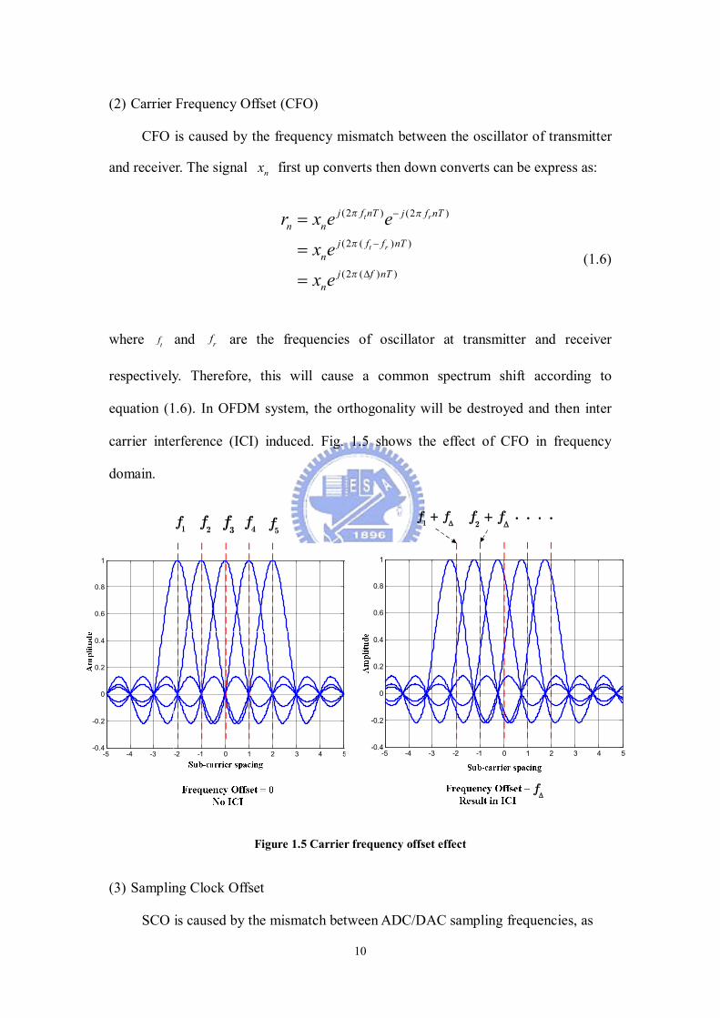
(2) Carrier Frequency Offset (CFO)
CFO is caused by the frequency mismatch between the oscillator of transmitter
and receiver. The signal nx first up converts then down converts can be express as:
(2 ) (2 )
(2 ( ) )
(2 ( ) )
t r
t r
j f nT j f nTn n
j f f nTn
j f nTn
r x e e
x e
x e
π π
π
π
−
−
∆
=
=
= (1.6)
where tf and rf are the frequencies of oscillator at transmitter and receiver
respectively. Therefore, this will cause a common spectrum shift according to
equation (1.6). In OFDM system, the orthogonality will be destroyed and then inter
carrier interference (ICI) induced. Fig. 1.5 shows the effect of CFO in frequency
domain.
-5 -4 -3 -2 -1 0 1 2 3 4 5-0.4
-0.2
0
0.2
0.4
0.6
0.8
1
-5 -4 -3 -2 -1 0 1 2 3 4 5-0.4
-0.2
0
0.2
0.4
0.6
0.8
1
1f 2f
3f 4f 5f
f∆
1f f∆
+2f f
∆+
Figure 1.5 Carrier frequency offset effect
(3) Sampling Clock Offset
SCO is caused by the mismatch between ADC/DAC sampling frequencies, as
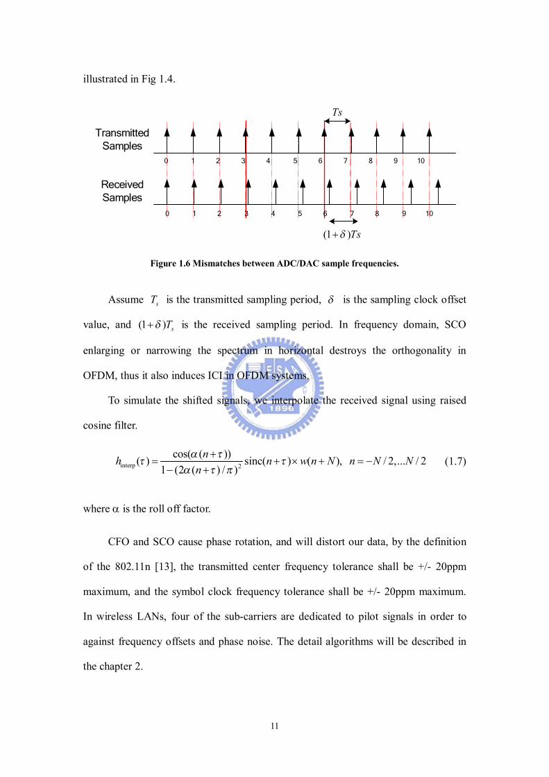
11
illustrated in Fig 1.4.
(1 )Tsδ+
Ts
TransmittedSamples
ReceivedSamples
0 1 2 3 4 5 6 7 8 9 10
0 1 2 3 4 5 6 7 8 9 10
Figure 1.6 Mismatches between ADC/DAC sample frequencies.
Assume sT is the transmitted sampling period, δ is the sampling clock offset
value, and (1 ) sTδ+ is the received sampling period. In frequency domain, SCO
enlarging or narrowing the spectrum in horizontal destroys the orthogonality in
OFDM, thus it also induces ICI in OFDM systems.
To simulate the shifted signals, we interpolate the received signal using raised
cosine filter.
interp 2
cos( ( ))( ) sinc( ) ( ), / 2,... / 21 (2 ( ) / )
nh n w n N n N Nn
α ττ τ
α τ π+
= + × + = −− +
(1.7)
where α is the roll off factor.
CFO and SCO cause phase rotation, and will distort our data, by the definition
of the 802.11n [13], the transmitted center frequency tolerance shall be +/- 20ppm
maximum, and the symbol clock frequency tolerance shall be +/- 20ppm maximum.
In wireless LANs, four of the sub-carriers are dedicated to pilot signals in order to
against frequency offsets and phase noise. The detail algorithms will be described in
the chapter 2.

12
1.3 Organization of this thesis
This thesis is organized as follows: the first chapter briefly introduces 802.11n
wireless LAN system and the channel model used for simulation. In chapter 2, the
algorithms of CFO mitigation, channel estimation, phase error tracking, and MIMO
detection will be described. Simulation results will be analyzed in Chapter 3. The
chapter 4 will show the architecture and the techniques of tri-mode hardware
implementation. Finally, a brief conclusion and future work will be presented in
chapter 5.
13
Chapter 2 Equalizer Design for WLAN
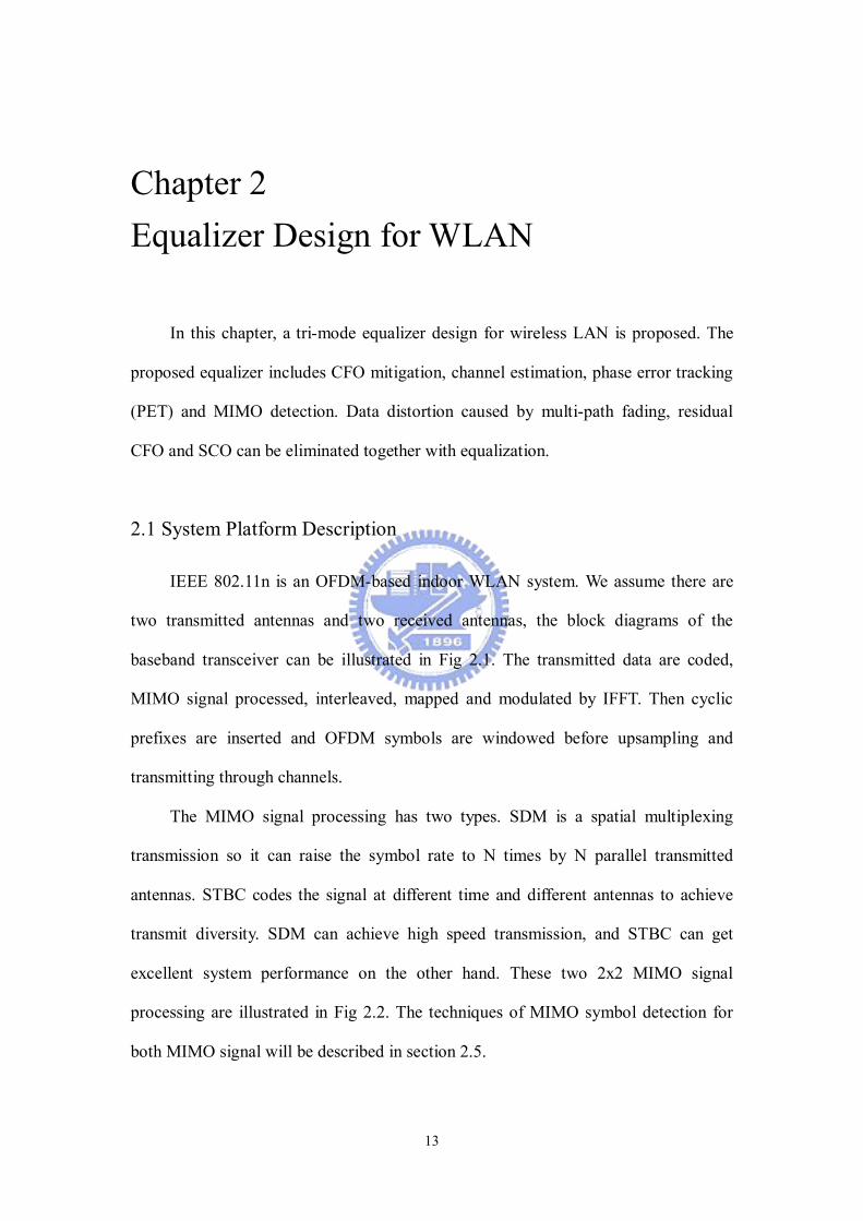
In this chapter, a tri-mode equalizer design for wireless LAN is proposed. The
proposed equalizer includes CFO mitigation, channel estimation, phase error tracking
(PET) and MIMO detection. Data distortion caused by multi-path fading, residual
CFO and SCO can be eliminated together with equalization.
2.1 System Platform Description
IEEE 802.11n is an OFDM-based indoor WLAN system. We assume there are
two transmitted antennas and two received antennas, the block diagrams of the
baseband transceiver can be illustrated in Fig 2.1. The transmitted data are coded,
MIMO signal processed, interleaved, mapped and modulated by IFFT. Then cyclic
prefixes are inserted and OFDM symbols are windowed before upsampling and
transmitting through channels.
The MIMO signal processing has two types. SDM is a spatial multiplexing
transmission so it can raise the symbol rate to N times by N parallel transmitted
antennas. STBC codes the signal at different time and different antennas to achieve
transmit diversity. SDM can achieve high speed transmission, and STBC can get
excellent system performance on the other hand. These two 2x2 MIMO signal
processing are illustrated in Fig 2.2. The techniques of MIMO symbol detection for
both MIMO signal will be described in section 2.5.
14
Mapping IFFT
Channel Estimation
De-interleave
Channel
CP & Windowing
FFT Remove CP
CodingMIMOSignal
processing
De-interleave
FFT Remove CP
Decoding
Mapping IFFT CP & Windowing
Data in
Data out
Interleave
Interleave
Demapping
Demapping
CFO Mitigation
MIMO Detection
Phase Error
Tracking
Stream 1
Stream 2
Tri-modeEqualizer
Stream 1
Stream 2
Figure 2.1 System block diagram.
...A C EB D F
* *
* *...A B C D
B DA C − −
Figure 2.2 2x2 MIMO signal processing.
While receiving, we assume perfect synchronization. Then cyclic prefixes are
removed, and signals are transferred to frequency domain by FFT. The following
step is equalization. The tri-mode equalizer consists of CFO mitigation, channel
estimation, phase error tracking and MIMO detection. The equalizer not only deals

15
with the channel effect but also compensates the CFO and SCO effects. The
algorithms of equalization will be described in detail in the following sections. After
equalization, de-mapping, de-interleaving and decoding are processed to recover
data.
2.2 CFO Mitigation
To enhance the accuracy of channel estimation, CFO mitigation is utilized to
reduce phase errors in the training fields which are used to estimate channels in the
mixed-mode of 802.11n.
In 802.11n, the preamble and the header have a Compatibility portion and a
High throughput portion for mixed-mode operation [12]. The Compatibility portion of
the mixed mode header consists of legacy signal field (L-SIG) can be decoded by
non-HT devices, as well as HT devices. What has been observed is that the pilots of
the L-SIG, HT-SIG and values in pilot locations in L-LFT in this preamble structure
can be utilized for CFO mitigation in HT mixed-mode operation. The training
symbols of 802.11n are shown as Fig 2.3.
L-STF L-LTF L-SIG HT-SIGHT-STF
HT-LTFs
Data
8u 8u 8u4u 4u4u perLTF
Compatibility portion High-Throughput portion
Figure 2.3 Training symbols of 802.11n.
We utilize the concept of the D-symbol estimation [14]. When the remained
CFO and SCO are relatively smaller or the Noise is very large, the differences of the
rotated phases between two adjacent symbols are very small, as illustrated in Fig.

16
2.4(a). This may result in poor estimation accuracy and in some cases may give
estimation results of the opposite sign. If we compare the phase rotation of the current
symbol with the next D symbol that delays D-symbol-interval, demonstrated as Fig.
2.4(b) and (c). the effects of noise may be reduced to some extent. From above
conclusions, the proposed CFO mitigation uses 2-symbol estimation to avoid this
problem thus gets better performance.
D
(a) (b)
(c)
Figure 2.4 The principle of D-symbol estimation [14]
The signal is compensated by CFO and the guard interval is removed before
FFT. Under consideration of residual CFO as f∆ , SCO as δ=(Ts’-Ts)/Ts, where Ts
is the sampling time and Ts’ is the offset sampling time. The post-FFT data stream
Yl,k,n at the k-th sub-carrier and the n-th receive antenna during l-th OFDM symbol
duration can be expressed as:
1
2 ( ) /, , , , , , , ,
stsl u g u
sts stssts
Nj l m T T T
l k n k l i k i n k l ni
Y e d H wπ φ
=
∆ += +∑ (2.1)

17
where , ,stsk i nH is the frequency response of the channel, gT is the guard interval, uT
is the duration of FFT, uf Tφ δ∆ ≈ ∆ ⋅ + , lm is the time-sample index of the first
element in the l-th symbol. , , stsk l id is the complex signal that is transmitted through the
k-th sub-carrier and the ists-th transmitted antenna during l-th OFDM symbol duration.
Wk,l,n is the noise caused from Additive White Gaussian Noise (AWGN), ICI, phase
noise and other non-ideal parameters. Let uf Tα = ∆ ⋅ be the phase shift caused from
the residual CFO in an OFDM symbol. There (2.1) can be re-written as
1
2 ( ) ( ) /, , , , , , , ,
stsl u g u
sts stssts
Nj l k m T T T
l k n k l i k i n k l ni
Y e d H wπ δ α
=
⋅ + += +∑ (2.2)
The received data after FFT at the pilot carrying sub-carriers in the L-LFT,
L-SIG and HT-SIG can be rewritten as
1
2 ( ) ( ) /( ) ( ), , , , , , , ,
stsl u g u
sts stssts
Nj l k m T T Tp p
l k n k l i k i n k l ni
Y e d H wπ δ α
=
⋅ + += +∑ (2.3)
where ( ), , sts
pk l id denotes the transmitted data in the pilot locations. While receiving
L-LFT, L-SIG HT-SIG, we can neglect the effects of SCO, i.e., uf Tφ∆ ≈ ∆ ⋅ for
convenient because SCO value is relative small compared with CFO at the beginning
of a packet. Assume that the channel response is almost static in the duration of a
packet which holds true for most indoor scenarios because the duration of a packet is
relatively shorter than the coherence time of indoor channel. The pilot patterns in the
L-SIG and HT-SIG are defined as the same as pilot patterns in 802.11a standard [15].
The pilot patterns in L-SIG and HT-SIG totally three symbols are exactly identical, so
we can directly compute the phase differences between any of the two consecutive
symbols. On the other hand, the phase differences between the first L-LTF symbol
and L-SIG need to be multiplied by an additional correct vector η . Define the first

18
received L-LTF symbol as Yλ . The 2-symbol phase difference ,1ˆstsiv and ,2ˆ
stsiv can be
expressed as:
*,1 2, , 4, ,
21, 7,7,21
ˆ ( ) sts sts stsi p i p i
pv Y Yλ λ+ +
=− −
= ×∑ (2.4)
*,2 , , 2, ,
21, 7,7,21
ˆ ( )sts sts stsi p i p i p
pv Y Yλ λ η+
=− −
= × ×∑ (2.5)
[ ] [ ]where = =7 21 -21 -7η η η η η 1 -1 1 -1 . The training symbols required for proposed
CFO mitigation are illustrated as Fig 2.5.
Figure 2.5 Training symbols required for proposed CFO mitigation.
The value of residual CFO is very small after coarse and fine CFO estimation
and compensation. To translate the complex-valued signals to phase, arctangent can
be approximated by a real divider. The double residual CFO value α ′ is obtained by
averaging over ,1ˆstsiv and ,2ˆ
stsiv . Finally, the residual CFO value α can be obtained
as:
,
,
ˆ[ ]
ˆ[ ]
sts
sts
stssts
i kk i
i kk i
v
vα
ℑ′ =
ℜ
∑∑
∑∑ (2.6)
ˆ 0.5α α ′= × (2.7)
L-STF L-LTF L-SIG HT-SIG HT-STF
HT-LTFs Data
8u 8u 8u4u 4u 4u perLTF
Compatibility portion High-Throughput portion
,1ˆstsiv,2ˆ
stsiv

19
In proposed design, the phase error of HT-LTFs can be compensated by counter
rotating the estimated phase in frequency domain with CORDIC modules.
2.3 Channel Estimation
Multipath fading is one of the data distortion issues in OFDM systems. The
wideband signal is transmitted over frequency-selective fading channel. The
preamble-based channel estimation is generally used under indoor channel because
the duration of a packet is relatively shorter than the coherent time, i.e. the channel is
assumed to be constant during a packet period. After obtaining the estimated channels,
equalization is applied to remove the multipath influence.
(1) SISO mode
In OFDM-based wireless LAN systems, preamble-based Zero Forcing channel
estimation is generally applied to estimate the channel frequency response for SISO
mode due to its advantage of low complexity. The pre-known signal is defined as ,l ka
in the preamble with l = λ,λ+1. Using the feature of the repeated structure in of
long preamble in frequency domain, we can average the result of twice Zero Forcing
estimations to suppress noise. The estimate of k-th sub-channel is generally given by
, 1,
, 1,
1ˆ2
k kk
k k
Y YH
a aλ λ
λ λ
+
+
= +
(2.8)
The pre-known signal ,l ka is 1 or -1 so the dividers can be avoided. Thus
Equation 2.8 can be modified as
, , 1,ˆ 0.5 ( )k k k kH a Y Yλ λ λ += × × + (2.9)

20
The estimated channels can be improved further by passing them through a
smooth filter. We use a three taps [0.25 0.5 0.25] FIR filter based on the correlative
property between adjacent sub-carriers. The smoothed channels are compared with the
results of the per tone estimation only in Fig 2.6.
Figure 2.6 Smooth the estimated channels with a 3 taps fir filter
(2) 2x2 MIMO modes (SDM-MIMO/ STBC-MIMO)
H22
H11a-a
aa
H11*(-a)+H12*aH11*a+ H12*a
H21*(-a)+H22*aH21*a+ H22*a
H21
H12
Figure 2.7 2x2 MIMO Channel Estimation for 802.11n
For 2x2 MIMO transmissions for 802.11n, there are two symbol durations for
HT-LTF. The relationship between the transmitted preambles and the combinations of
0 1 0 2 0 3 0 4 0 5 0 6 0 7 00
0 . 2
0 . 4
0 . 6
0 . 8
1
1 . 2
1 . 4
1 . 6
S u b -c a rrie r
Am
plitu
de
S N R = 2 0
P e r To n e E s t im a t io nS m o o t h e d

21
the signals in receiver are illustrated as Fig. 2.7. We note that the HT-LTF is
transmitted in Alamouti form for 2x2 MIMO. The pre-known signal is defined as ak in
the preamble, and the received preamble signals of k-th sub-channel can be expressed
as:
1, 6, 11, 12,2 1
21, 22,2, 6,
r k k k k
k kr k k
Y H H aN
H HY aλ
λ
+×
+
= +
(2.10)
1, 7, 11, 12,2 1
21, 22,2, 7,
r k k k k
k kr k k
Y H H aN
H HY aλ
λ
+×
+
− = +
(2.11)
where 1, ,r l kY and 2, ,r l kY are the received signals of l-th symbol and k-th sub-channel
at receiving stream 1 and stream 2 respectively. We can observe that all channel
frequency responses can be obtained by simple linear combinations.
After linear combination, the 2x2 MIMO channel estimates of k-th sub-channel
are given by:
1, 6, 1, 7, 1, 6, 1, 7,2 2,
2, 6, 2, 7, 2, 6, 2, 7,
1ˆ 0.5 r k r k r k r kk
r k r k r k r kk
Y Y Y YH
Y Y Y Yaλ λ λ λ
λ λ λ λ
+ + + +×
+ + + +
− + = × × − +
(2.12)
The pre-known signal ak is 1 or -1 so complex dividers can be avoided. Thus
equation 2.12 can be modified as
1, 6, 1, 7, 1, 6, 1, 7,2 2,
2, 6, 2, 7, 2, 6, 2, 7,
ˆ 0.5 r k r k r k r kk k
r k r k r k r k
Y Y Y YH a
Y Y Y Yλ λ λ λ
λ λ λ λ
+ + + +×
+ + + +
− + = × × − +
(2.13)
2.4 Phase Error Tracking
Carrier Frequency offset (CFO) and sampling clock offset (SCO) are the other
two major data distortion issues in OFDM systems. Though CFO has been mitigated
by coarse and fine CFO estimation in time domain, the CFO error (or residual CFO)

22
in data portion still can not be neglected. Residual CFO and SCO rotating the received
data in constellation diagrams cause great data errors while receiving. Phase error
tracking (PET) is generally applied to trace the phase rotation caused by residual CFO
and SCO; Fig. 2.8 shows the 64QAM constellation with and without PET.
(a) (b)
Figure 2.8 64QAM data constellation: (a) without PET (b) with PET
2.4.1 Carrier Frequency Offset Tracking
In this section, an Least Mean Square (LMS) based adaptive CFO tracker is
proposed. Considering the integration of the three modes, different but similar
algorithms are used here in order to get a good trade-off between performance and
computational complexity. The proposed CFO tracking has three steps to complete the
adaptive recursion.
Step 1. Pilot Pre-compensation
When the packet length is long, the phase error caused by residual CFO may
exceed the ±π range. This will cause large estimation error while tracking residual
CFO using conventional PET. The pilot pre-compensation concept [16] is utilized to
solve this problem. The received data after pilot pre-compensation is written as:

23
1,ˆ
, , , ,
1, 2; 21, 7, 7, 21
m k
sts sts
jm i k m i k
i ksts
Y Y e λφλ λ
+ −−+ +
= = − −
′ = ⋅ (2.14)
where 1ˆ
mλφ + − is the phase error at (λ+m-1)-th symbol.
Step 2. Phase Estimation
After pilot pre-compensation, the detected pilot phase is the difference between
two adjacent OFDM symbols. The detected pilot phases in complex form can be
written as:
, , , , , , , ,1
1, 2; 21, 7, 7, 21
ˆˆ ( )TX
sts sts sts sts TX
TX
N
m i k m i k m i k i i ki
i ksts
u Y conj P Hλ λ λ+ + +=
= = − −
′= ⋅ ∑ (2.15)
where , ,stsm i kPλ + is the transmitted pilot value of k-th sub-carrier of ists-th transmitted
antenna during (λ+m)-th OFDM symbol duration. The pilots occupies at k = -21, -7, 7,
21 in each OFDM symbol.
To average the phases over receiving streams and pilot sub-carriers, We use two
different methods to obtain mean phase error in the three modes. Linear Least Square
(LLS) [14] is utilized in SDM-MIMO and STBC-MIMO modes, and Weighted Least
Square (WLS) [17] is utilized in SISO mode on the other hand. LLS has the
advantage of low computational complexity, but has bad performance in the condition
of few pilot numbers, especially in low SNR conditions. WLS has better performance
than LLS by using the information of signal’s power but pays the price of more
complexity in hardware. In the 2x2 SDM-MIMO and STBC-MIMO modes, there are
eight pilots from two data streams totally, but there are only four pilots for PET
utilization in SISO mode. For these reasons, we use WLS and LLS to estimate the
phase rotations from residual CFO in SISO mode and SDM-MIMO/STBC-MIMO

24
modes, respectively.
Linear Least Square for SDM-MIMO/STBC-MIMO modes:
, ,21, 7,7,21
ˆ ˆsts
sts
m m i ki k
u uλ λ+ +=− −
= ∑ ∑ (2.16)
ˆ[ ]ˆ[ ]
mm
m
uu
λλ
λ
α ++
+
ℑ′ =ℜ
(2.17)
Weighted Least Square for SISO mode:
2
, ,m k m kw Yλ λ+ += (2.18)
, ,,
, ,
ˆ[ ]ˆ[ ]
sts
sts
m i km k
m i k
uu
λλ
λ
α ++
+
ℑ=
ℜ% (2.19)
, ,21, 7,7,21
,21, 7,7,21
m k m kk
mm k
k
w
w
λ λ
λλ
αα
+ +=− −
++
=− −
′ =∑
∑
%
(2.20)
where wλ+m,k is the weighted coefficients of k-th sub-carrier during (λ+m)-th OFDM
symbol duration and it is calculated from the power of received data, mλα +′ is the
estimated phase shift from residual CFO between (λ+m-1)-th and (λ+m)-th symbols.
To get the pilot phase difference between two adjacent symbols from complex value
u , the arctangent operation can be approximated by a real divider because the phase
difference values are very small between two adjacent symbols.
Step 3. Recursive Adjustment
In step 3, we calculate the error vector to update the residual CFO value in
current symbol.
1ˆm m mλ λ λα α+ + + −′Θ = − (2.21)
1 0ˆ ˆm m mλ λ λα α µ+ + − += + Θ (2.22)

25
ˆ ˆ ˆ( ) ( )
2,3, 4... , SISO mode 8,9,10... , SDM-MIMO/STBC-MIMO modes
m m mk m
m
λ λ λφ δ α λ+ + += ⋅ + ⋅ +
=
(2.23)
where u0 is the step size which is chosen to the power of two for implementation
consideration. Θλ+m is the error vector at (λ+m)-th symbol, ˆ mλα + is the new updated
phase shift caused by residual CFO at (λ+m)-th symbol, ˆ mλδ + is the estimated phase
shift caused by SCO at (λ+m)-th symbol and ˆ mλφ + is the estimated phase error at
(λ+m)-th symbol. The method to obtain ˆ mλδ + is described at next section.
The first estimate of residual CFO for SISO mode can be obtained by
1, ,
1
ˆ ˆ( )ˆ
52
k kk
λ λ
λ
φ φα
+
+
−=
∑ (2.24)
The first estimate of residual CFO for SDM-MIMO/STBC-MIMO modes can be
obtained from in (2.7):
7ˆ ˆλα α+ = (2.25)
2.4.2 Sampling Clock Offset Tracking
Assume that carrier frequency and sampling time are generated by the same
reference oscillator in receiver as suggestion of 802.11n specification [13]. The phase
shifts caused from CFO ε and SCO δ have the following relationship:
( )c FFTf Tε δ= ⋅ ⋅ (2.26)
where fc is carrier frequency and TFFT is the duration of FFT.
26
2.5 MIMO Detection
In this section, one tap channel equalizer for SISO mode and two types of 2x2
MIMO symbol detectors for SDM-MIMO and STBC-MIMO are introduced
respectively. The complexity in hardware is important considering implementation.
Zero Forcing (ZF) having low complexity is generally used in SISO mode for
wireless LAN. The optimal SDM-MIMO symbol detector is the maximal likelihood
(ML) detector, but its complexity increases exponentially with number of transmit
antennas and modulation order [18]. Sphere decoding scheme has the main
disadvantage of lots delay. Vertical Bell Labs Layered Space-Time (V-BLAST) is a
sub-optimal solution also requires lots of computational complexity on
ordered-successive-interference cancellation (OSIC). On the other hand, minimal
mean square error (MMSE) provides a good trade-off between performance and
complexity for SDM-MIMO detection. The data encoded by STBC has an advantage
of low complexity in receiver. The data is transmitted in Alamouti form for 2x2
STBC-MIMO mode, so maximal likelihood (ML) symbol detection can be utilized to
decode STBC-MIMO signals.
2.5.1 Zero Forcing channel equalizer for SISO mode
The ZF channel equalizer can be expressed as
( )ˆ ( ) ˆk
Y kX kH
= (2.27)
where ˆkX is the equalized signal of k-th subcarrier. In Equation (2.27), received data
Yk is divided by the estimated Channel Frequency Response to eliminate multipath
fading.

27
2.5.2 Minimal Mean Square Error SDM-MIMO Symbol Detection
The channel matrix coefficients of the k-th subcarrier are given by:
1, 3,
2, 4,
k kk
k k
h hH
h h
=
(2.28)
It operates under the same subcarrier in the following, so we let hm,k=h,m, Hk=H.
Equation (2.28) can be re-written as:
1 3
2 4
h hH
h h
=
(2.29)
The receiving signals can be modeled as:
Y(k)=H X(k)+N(k)⋅ (2.30)
where Y(k) and X(k) are the received and transmitted signals of k-th subcarrier
respectively, and N(k) is the noise term.
We define an error vector e(k) which is the difference between the transmitted signals
and the received signals which have passed through MMSE filter. e(k) is defined as :
He(k)=X(k)-G Y(k) (2.31)
where G is the MMSE filter. We define the cost function J as:
HJ=E{e (k)e(k)} (2.32)
Because J is a scalar value, it can be re-written as:
HJ=tr[E{e(k)e (k)}] (2.33)
To minimize cost function J, we set zeros to the complex gradient vector J∇ , then
Wiener-Hopf equation is obtain as:

28
HYY XYG R =R (2.34)
where
YY XYR { ( ) ( ) } R { ( ) ( ) }H HE Y k Y k E X k Y k= = (2.35)
where RYY is the covariance of the received signals and RXY is the cross-correlation
of the transmitted and received signals.
From Equation (2.34), we can obtain MMSE filter as:
11r r
HN NG HH I H
SNR
−
× = +
(2.36)
and Equation (2.36) can be re-written as:
11t t
HN NG H H H I
SNR
−
× = +
(2.37)
The noise power can be calculated as:
1 12 2 21 2 1 2
0 0
1 1( ) ( ) ( ) ( ) 2N N
p pk k
Y k Y k N k N kN N
σ− −
= =
− = ∆ − ∆ ≈∑ ∑ (2.38)
1 221 2
0
1ˆ ( ) ( )2
N
p pk
Y k Y kN
σ−
=
= −∑ (2.39)
Finally, we can obtain the decoding signal as:
ˆ ( ) ( )HX k G Y k= ⋅ (2.40)
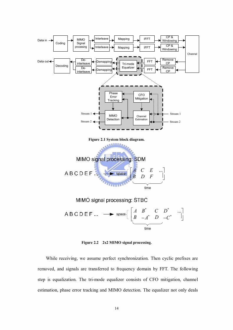
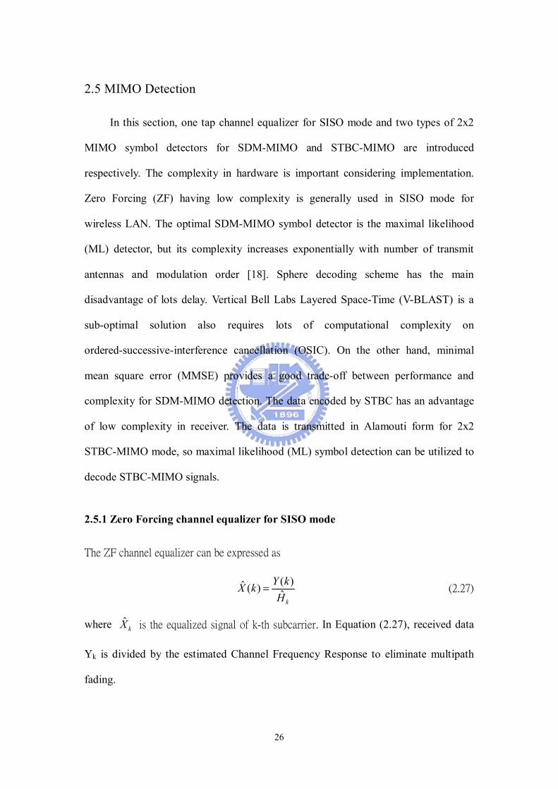
The constellations after MMSE detection are shown as Fig. 2.9.
29
(a) SNR=14 (b) SNR=28
Figure 2.9 Constellation diagram of MMSE detection under different SNR.
2.5.2 Maximal Likelihood STBC-MIMO Symbol Detection
Example of the 2x2 STBC-MIMO transmissions:

30
Table 2.1 Transmitted signals for 2x2 STBC-MIMO
TX1 TX2
Symbol 1 S0 S1
Symbol 2 -S1* S0
*
The receiving signal for 2x2 STBC-MIMO can be express as:
0 00 010 1
* *1 11 0 30 0
tx
y nhs ss s hy n
= + −
64748
(2.41)
0 01 2 10 1
* *1 11 01 4 1
tx
y h ns ss sy h n
= + −
64748
(2.42)
where yij represents the receiving signal of i-th receiving antenna at j-th symbol.
Equations (2.41) and (2.42) can be transferred as:
0 00 001 3
* *1* 1*3 10 01
tx
y nsh hh hy ns
= + −
64748
(2.43)
0 001 12 4
* *1* 1*4 21 11
tx
sy nh hh hy ns
= + −
64748
(2.44)
Then Equations (2.43) and (2.44) are multiplied by the Hermition transpose of the
channel gain matrix, respectively:
0 0* *2 2 2 2 00 11 3 2 4
1 2 3 4 * *1* 1*3 1 4 20 11
( )ys yh h h h
h h h h Nh h h hy ys
+ + + = + + − −
(2.45)
where N is the linear combination of noise. We can obtain the estimated signal by
dividing 2 2 2 21 2 3 4h h h h+ + + . The constellations after ML detection are shown as
Fig. 2.10.

31
(a) SNR=10 (b) SNR=18
Figure 2.10 Constellation diagram of ML detection under different SNR.
32
Chapter 3 System Simulation and Performance Analysis
In this chapter, we will discuss the design flow, system platform and
performance for the proposed design. A complete baseband system platform on
MATLAB is established complaint to 802.11n draft to verify the proposed design.
Channel estimation accuracy, PET performance and PER for overall system will be
simulated and be compared with conventional approaches.
3.1 Design and Verification Flow
In design and verification flow as shown in Fig 3.1, we first have to understand
the design requirements. Second, appropriate algorithms can be determined for
proposed design, and then be simulated in float point on MATALB to evaluate
whether it meets the specification requirements. Next, word length in each operation
will be determined to compromise between performance and complexity in fixed
point simulation. The simulation on MATLAB is completed here if the performance
of fixed point simulation meets specification requirements. The RTL code is
developed according to the fixed point simulation and then is synthesized by XST
Synthesizer built in Xilinx ISE. Finally the flow is completed after FPGA verification.
33
Figure 3.1 Design and verification flow
Figure 3.2 The system platform on MATLAB
3.2 System Platform on MATLAB
Our system platform on MATLAB is illustrated as Fig 3.2. The platform is built
based on IEEE 802.11n draft and the simulated channel has been introduced in
34
chapter 1. The parameters of the system environment are set according to IEEE
802.11 TGn Comparison Criteria 67 [6]:
n Trace-back length of Viterbi decoder is 128.
n No smoothing filter for channel estimation, i.e., per tone estimation
n PPDU length is 1000 bytes.
n SNR is calculated as ensemble averaged SNR.
n When the number of packet error reaches to 100, then quit from this
loop.
n 20,000 seeds of channel realization are used
Physical layer impairments added in our platform include
n IM2 (Carrier frequency offset)
Offset value is -20ppm, and sampling clock offset is also added.
n IM6 (Antenna Configuration)
Antenna configuration is linear array and distance between adjacent
two antennas is a half wavelength.
In our simulations, we have one FEC encoder and two spatial streams. Rate 1/2
convolutional coding is employed. Also, 800 ns Guard interval is used. The IEEE
indoor MIMO WLAN channel model ‘D’ [5] in the condition of non line of sight
(NLOS) is applied. No beamforming is considering in our system.
3.3 Performance Analysis
The performance of the tri-mode equalizer for 802.11n will be simulated and
analyzed in this section. We will focus on the 10% PER in system performance, which
is the requirement of IEEE 802.11n standard.
35
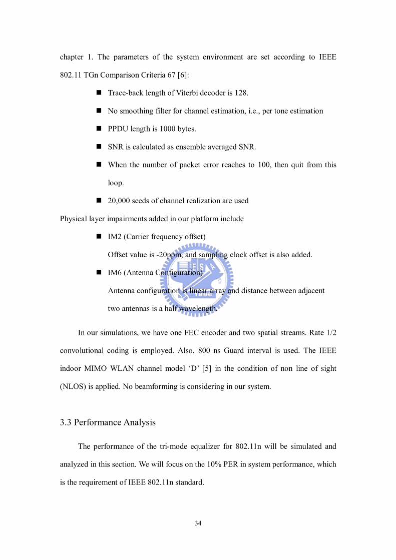
3.3.1 Channel Estimation Accuracy Analysis
Channel estimation accuracy is highly related to the effects of residual CFO in
preamble portion for 802.11n as introduced in chapter 2. HT-LTFs are use to estimate
MIMO channels in preamble based channel estimation, and the residual CFO in
HT-LTFs can be suppressed by CFO mitigation. So channel estimation accuracy is
used to analyze the performance of CFO mitigation. We first define the mean channel
estimation error as
, , , ,1 1
ˆ /( )M N
i j k i j ki j
Mean H H MN= =
−
∑∑ (3.1)
where , ,ˆ
i j kH is the ij-th element of estimated channel frequency response of k-th
subcarrier and M×N is the dimension of kH . Fig. 3.3 shows the residual CFO effects
on channel estimation error under different CFO mitigation algorithms for 802.11n
(2x2 system) on a TGn D channel.
10 12 14 16 18 20 22 24 26 28 3010
-2
10-1
100
Mean channel estimation errors at different SNR
SNR per receive antenna, dB
Mea
n C
han
nel
est
imat
ion
err
ors
per
sam
ple
proposed
w/o mitigationref [4]
ideal cfo esti.
Figure 3.3 Mean channel estimation errors vs. SNR under different
CFO mitigation algorithms.

36
The proposed CFO mitigation achieves 1.0~4.0dB SNR gain in mean channel
error compared with conventional one which is without CFO mitigation. Compared
with the method used in [4], there are still 0.5~2.0dB SNR improvement in mean
channel error, so the proposed CFO mitigation algorithm increases the accuracy of
channel estimation effectively.
3.3.2 Phase Error Tracking Performance Analysis
CFO is one of the main factors to degrade system Packet Error Rate (PER)
performance. In order to verify the PET performance, the design is simulated under
40ppm CFO, which is standard requirement. The transmission is under QPSK and 1/2
coding rate. Fig 3.4 shows that different PET algorithms are compared for 802.11n
(2x2 system) on PER performance. We notice that conventional weighted average
method [14] can not get good performance and mean average method [16] is even
worse. As mentioned in chapter 1, the pilot-based PET can not suppress noise enough
to get a satisfied PER performance due to few pilot numbers in WLAN systems,
Figure 3.4 Compare PET Algorithms at 2x2 MIMO, QPSK, ½ Code rate.
4 6 8 10 12 14 16 18 2010
-2
10-1
100
101
Compare PER
SNR
mean average
proposed method
weighted average
Ideal CFO Estimation
PER = 10%

37
especially in low SNR region. There are only 4 pilots can be utilized per data symbol
in one data stream for wireless LAN systems. On the other hand, the proposed
adaptive CFO tracking algorithm suppresses the PER loss due to residual CFO within
0.2 dB for 802.11n (2x2 system) compared with ideal CFO estimation. From Fig. 3.4,
the proposed adaptive PET achieves 3.0 dB gains than weighted average one at 10%
PER requirement. We can conclude the proposed PET increases the system
performance a lot.
3.3.3 System Performance
To verify the complete system performance of the proposed tri-mode channel
equalizer, PER of a complete IEEE 802.11n basdband processor are simulated with
the TGn proposed indoor wireless channel model D and non-ideal impairments of
40ppm CFO and 40ppm SCO in receiver.
The required SNR for SISO and SDM-MIMO modes to achieve 10% PER are
listed in Table 3.1. The proposed baseband system can achieve 0.2~3.8dB and
0.2~1.2dB SNR gain compared with TGn proposed results [19] and [20], respectively.
Table 3.1 PER Performance Comparison on SISO/SDM
35.526.514N/ARequired SNR, TGn [1]
10
10.2
N/A
26
½
2x2
4QAM
9
33.324.521.8Required SNR, This Work
33.324.421Required SNR, Ideal
33.52523Required SNR, PLL Based [2]
1307839Data Rate( Mbps)
5/6¾¾Coding Rate
2x22x21x1MIMO
64QAM
16QAM
16QAM
Modulation
15124MCS
35.526.514N/ARequired SNR, TGn [1]
10
10.2
N/A
26
½
2x2
4QAM
9
33.324.521.8Required SNR, This Work
33.324.421Required SNR, Ideal
33.52523Required SNR, PLL Based [2]
1307839Data Rate( Mbps)
5/6¾¾Coding Rate
2x22x21x1MIMO
64QAM
16QAM
16QAM
Modulation
15124MCS

38
Higher performance can be obtained in the proposed baseband receiver because
the effects of CFO are outstandingly suppressed by the proposed CFO mitigation and
adaptive PET.
The PER curves of different transmission modes for STBC-MIMO (2x2 system)
are shown in Fig. 3.5. System constraint for 802.11a and the required SNR to meet
10% PER for STBC-MIMO for 802.11n are listed in Table 3.2. We note that much
better performance can be obtained compared with legacy SISO systems due to space
diversity of an additional antenna. Especially in low SNR region, outstanding
performance can be achieved, thus suitable for low data rate and high performance
transmission.
PE
R
Figure 3.5 PER performance on STBC mode under TGn channel model D,
40ppm CFO and 40 ppm SCO

39
Table 3.2 System constraint for 802.11a and the required SNR to meet 10% PER
for STBC-MIMO for 802.11n
802.11a STBC-MIMO for 802.11n
Data Rate System Constraint
(dB) Data Rate
Required SNR
(dB)
6 9.7 6.5 3
9 10.7 13 6
12 12.7 19.5 8
18 14.7 26 10
24 17.7 39 14
36 21.7 52 18
48 25.7 58.5 20
54 26.7 65 21

40
Chapter 4 Hardware Implementation
In chapter 2, we proposed a tri-mode equalizer for OFDM-based wireless LAN.
Considering hardware implementation efficiently for tri-mode equalizer design, many
shared-architectures based on common algorithms and different working timing are
derived and utilized in this chapter.
4.1 Common Architecture Design for Tri-mode Equalizer
We proposed a common architecture design for tri-mode equalizer as shown in
Fig. 4.1. We note that a Coordinate Rotation Digital Computer (CORDIC) is used to
compensate phase errors in our equalizer design. CORDIC is a well-known iterative
method for the computation of vector rotation. Compared to Look-up-tables (LUTs),
CORDIC reduces the complexity by using adders, shifters, and comparators.
CORDICFFT DeMUX
CFOMitigation
ChannelEstimatio
nPET
MUX DeMUXMIMO
Detection
to Demapping
HRAM
Tri-mode Equalizer
Control
Figure 4.1 Tri-mode equalizer architecture

41
The signals after FFT will go in CFO mitigation first for SDM-MIMO and
STBC-MIMO modes or will bypass it for SISO mode, and then the estimated residual
CFO in HT-LTFs will be compensated by CORDIC. The High-Throughput Long
Training Fields (HT-LTFs) are used to estimate MIMO channels for
SDM-MIMO/STBC-MIMO modes and Legacy Long Training Field (LLF) is used to
estimate channel for SISO mode. The estimated channels then will be saved in RAMs.
With estimated channels, PET can track the phase errors caused by residual CFO and
SCO. Then send to CORDIC in the same manner to compensate phase errors in data
portion. Here we notice that one CORDIC can be fully utilized for two times because
CFO mitigation and PET work at different timings. Finally, the data after CORDIC
will be equalized by MIMO detection. In the following section, the modules in
tri-mode equalizer will be described in detail.
4.2 Modules Design
4.2.1 CFO Mitigation Module Design
The proposed architecture of CFO mitigation is shown as Fig. 4.2.
CFO Mitigation
7...0Stream1 pilot ( )*
7...0Stream2 pilot ( )*
η D
[ ]ℑ
[ ]ℜ
RealDivider
>>
To CORDIC
Figure 4.2 The proposed CFO mitigation architecture
42
The proposed CFO algorithm has the main advantage of low complexity as
mention in chapter 2. To further reduce the area consumptions, we note a feature that
CFO mitigation operates during receiving preambles and PET and MIMO detection
work during receiving data portion. For this reason, all the main components i.e. the
two marked complex multipliers and the real divider shown in Fig.4.2 can share the
hardware resources with MIMO detection and PET respectively, so it achieves very
low complexity in hardware.
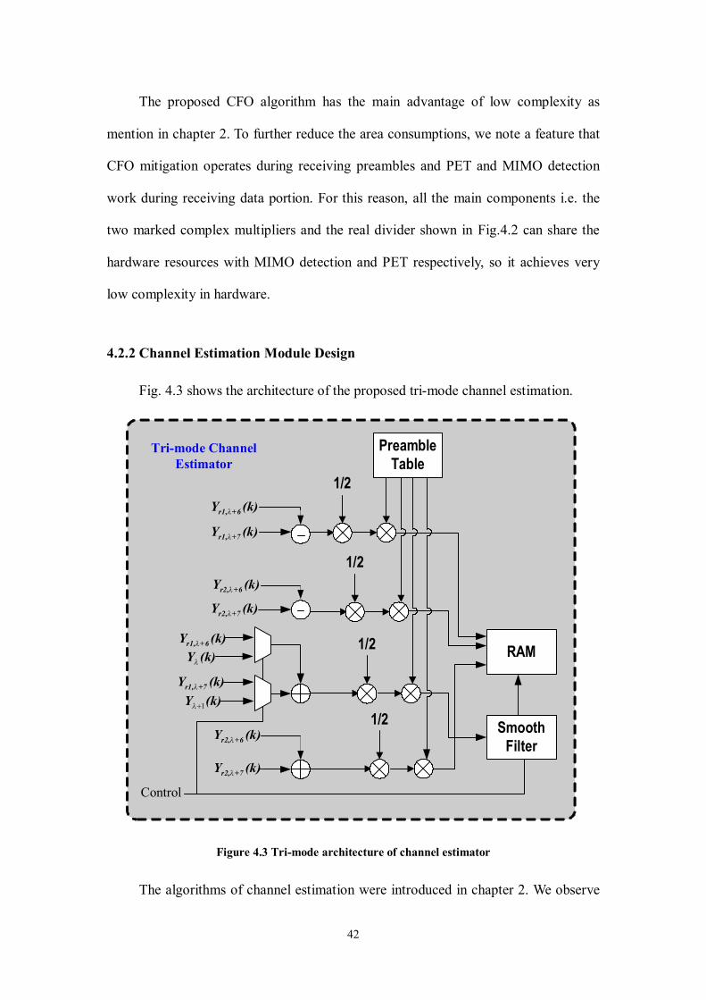
4.2.2 Channel Estimation Module Design
Fig. 4.3 shows the architecture of the proposed tri-mode channel estimation.
λr1, +6Y (k)
λr1, +7Y (k)
λr2, +6Y (k)
λr2, +7Y (k)
λr1, +6Y (k)
λr1, +7Y (k)
λr2, +6Y (k)
λr2, +7Y (k)
PreambleTable
1/2
1/2
1/2
1/2
RAMλY (k)
1λ+Y (k)
Tri-mode Channel Estimator
SmoothFilter
Control
Figure 4.3 Tri-mode architecture of channel estimator
The algorithms of channel estimation were introduced in chapter 2. We observe

43
that the operation in Equation (2.9) can be totally included in Equation (2.13) so
shared architectures of channel estimation is used for three modes. The estimated
channel frequency response (CFR) is then sent to a smoothing FIR filter with three
taps [0.25 0.5 0.25] for SISO mode, or is saved to RAM without smoothing for
SDM-MIMO and STBC-MIMO modes on the other hand.
4.2.3 Phase Error Tracking Module Design
The proposed architecture of CFO tracking is shown as Fig. 4.4. Same as the
steps of the proposed algorithm mentioned in chapter 2, we divide the architecture to
three portions, i.e. pilot pre-compensation, phase estimation and recursive adjustment.
In the pilot pre-compensation portion, the phases of pilots in both data streams are
compensated using CORDIC modules. After pilot pre-compensation, the detected
pilot phase is the difference between two adjacent OFDM symbols. In the phase
estimation portion, the architectures of the weighted average phase estimation for
SISO mode and the mean average phase estimation for SDM-MIMO/STBC-MIMO
modes are combined together. In addition to mean average phase estimation, there are
only two de-multiplexers are addition to the proposed architecture. Most of the
components are shared, so this architecture increases little complexity in hardware.
Finally, in the recursive adjustment, error vector at current symbol is calculated and
the estimated residual CFO is updated. Using the relationship mentioned in equation
(2.26), the estimate of SCO can be obtained from CFO. Then the total phase error is
sent back to pilot pre-compensation for next symbol duration and is sent to CORDIC
modules outside to correct phase errors in data potion.

44
,1,
mr
pY λ
+
1,ˆ
,2,
mk
jm
rk
Ye
λφλ
+−
−+
,2,
mr
pY λ
+
[]
ℑ
[]
ℜ
0µ
mλ
+
1,ˆ
mk
λφ+
−
1,ˆ
,1,
mk
jm
rk
Ye
λφλ
+−
−+
ˆm
λα
+
ˆm
λφ+
1ˆ
mλ
α+
−
mλ
+Θ
,1,ˆ
mk
u λ+
,2,
ˆm
ku λ
+
ˆm
u λ+
mλ
α+′
1ta
n−
2
δ
ˆm
λα
+
Figure 4.4 The proposed Tri-mode CFO tracker architecture
45
4.2.4 MIMO Detection Module Design
The channel matrix coefficients of the k-th subcarrier are given by:
1, 3,
2, 4,
k kk
k k
h hH
h h
=
(4.1)
It operates under the same subcarrier in the following, so we let hm,k=h,m, Hk=H. The
Equation (4.1) can be re-written as:
1 3
2 4
h hH
h h
=
(4.2)
From Equation (2.37), the MMSE filter for SDM-MIMO is:
11t t
HN NG H H H I
SNR
−
× = +
(4.3)
We can re-write Equation (4.3) as
* * * * * * * * * *1 4 4 4 3 2 2 3 3 3 1 4 1 2
* * * * * * * * * *3 2 2 2 1 4 4 1 1 1 3 2 3 4
( ) ( ) ( ) ( )1( ) ( ) ( ) ( )
H h h h h h h h h h h h h h hG
g h h h h h h h h h h h h h hα
− − = + − −
(4.4)
* * * * * *1 1 4 4 2 2 3 3 1 4 2 3
* * * * * * 22 3 1 4 1 1 2 2 3 3 4 4
( )( ) ( )( ) ( )( ) ( )( ) ( )g h h h h h h h h h h h h
h h h h h h h h h h h hα α
= + −
− + + + + + (4.5)
where α is the reciprocal of SNR per receiver, and we ignore the effect of 2α
because it is relatively small. The output after MMSE filter can be written as
ˆ ( ) ( )HX k G Y k= ⋅ (4.6)
In SISO mode transmission, all the channel frequency responses of h2, h3 and h4 are
zeros. We observe Equation (4.5) can be simplified as zero forcing for SISO mode
1
( )ˆ ( ) Y kX kh
= (4.7)
On the other hand, STBC detection for STBC-MIMO can be expressed as

46
0 0* *2 2 2 2 00 11 3 2 4
1 2 3 4 * *1* 1*3 1 4 20 11
( )ys yh h h h
h h h h Nh h h hy ys
+ + + = + + − −
(4.8)
The output of STBC detection can be written as
0 0* *00 11 3 2 4
2 2 2 2 * *1* 1*3 1 4 20 11 1 2 3 4
ˆ 1ˆˆ ( )
yx yh h h hX
h h h hy yx h h h h
= = + − −+ + + (4.9)
From above derivation, we can find some similarity between MMSE detection
and STBC detection. Both detections need channel coefficients 2 2 2 21 2 3 4h h h h+ + + ,
and 2x2 matrix multiplications are required. From above observations, the proposed
tri-mode MIMO detection is shown as Fig. 4.5.
Figure 4.5 Tri-mode MIMO Detector architecture
While designing the proposed architecture, we notice that the channel coefficients
2 2 2 21 2 3 4h h h h+ + + and matrix multiplier can be shared in hardware. The
coefficients which MMSE and STBC need are calculated first at the beginning, and
then are sent to divider and matrix multipliers. The incoming data are first divided by
g as given in Equation (4.5), and then pass through matrix multiplier for SISO and
SDM-MIMO modes. In STBC-MIMO mode, some additional operations are need

47
while receiving. Data is encoded across symbols so a delay line is needed to save data
of last symbol. An extra matrix multiplier and an adder are also needed for 2x2 STBC
operations in ML MIMO detection. To further reduce the complexity in hardware, we
note that there is only one operation in MMSE/STBC coefficients calculation during a
packet length so the additional matrix multiplier (lower position in the Fig. 4.5) can
share complex multipliers with coefficients calculation block for STBC-MIMO mode.
4.2.5 CORDIC Module Design
CORDIC is used for phase rotation in the proposed architecture. General methods to
realize this function needs LUTs, complex multipliers. CORDIC reduces complexity
in hardware by usage of simple components like adders, comparators and shifters.
CORDIC has another advantage that it can be implemented with pipeline structure
easily because of its similar operation in each stage. The i-th iterative formula is
defined as
( 1) ( )1 2( 1) ( )2 1
ii
ii
x i x iuy i y iu
−
−
+ = + −
(4.10)
with
1tan (2 )iiθ − −= (4.11)
where the number of stage i=0,1,2,…,N-1, [xi yi]T is the input vector, [xi+1 yi+1]T is the
output vector, and ui is use to determine the direction of rotation and is given by
[ ( )]iu sign z i= − (4.12)
where z(i) is the phase rotated in i-th stage. After finishing the rotation of N stages,
the output vector need to be multiplied by the factor
12 2
0
1
1 (2 )N N
i
i
A −−
=
=+∏
(4.13)

48
to maintain the same amplitude as input vector. The CORDIC cell structure of i-th
stage is illustrated as Fig. 4.6.
-Sign[z(i)]
+/-
-Sign[z(i)]
+/-
-Sign[z(i)]
+/-
y(i+1)
x(i+1)x(i)
y(i)
tan-1 (2-i)
>> i
>> i
θi θi+1
Figure 4.6 The architecture of CORDIC cell at i-th stage
The overall architecture of CORDIC is shown as Fig. 4.7
Figure 4.7 The architecture of CORDIC module
While implementing CORDIC, there are issues should be considered. The phase
range of the input angle should be between -π ~ π , or errors will occur. Another issue
is that the angle value between -π ~ π is hard to be expressed in 2’s complement form.
Also, the angular adder can not be implemented by conventional adder and should be
redesign. In the proposed design, the input angle of CORDIC is normalized with the
factor 2/π, so the range of the phase will be normalized from -2 to 2.
The angle after normalizing is as shown in Fig. 4.8. It shows that the phases can
be easily represented as 2’s complement form. The most important of all, overflow

49
issue can be completely solved in this method. For example, the conventional
calculation result of π/2 + 3π/4 = 5π/4 ( = -3π/4), the proposed calculation result
obtains result of 01.0(2) + 01.1(2) = 10.1(2) correctly.
00.0(2)
00.1(2)
01.0(2)
01.1(2)
10.0(2)
11.1(2)
11.0(2)
10.1(2)
Figure 4.8 The normalized angle
4.3 Implementation Results
4.3.1 Fixed-point Simulation
Before developing RTL code, we have to determine the bit numbers of each
operation. To reduce hardware complexity, fewer bit numbers are better. However,
hardware cost and system performance are trade-off in hardware implementation. The
bit numbers of main modules in tri-mode equalizer are listed in Table 4.1.
After the bit numbers of each operation are determined, fixed-point simulation
are utilized to evaluate the system performance in hardware. The performance
comparison of floating point and fixed point simulations in the highest data rate
condition of 64QAM and 5/6 coding rate under TGn channel model D, 40ppm CFO

50
and 40ppm SCO for 2x2 SDM-MIMO are shown as Fig. 4.9. We can note that in Fig.
4.9, there is only 0.3 dB performance loss in fixed-point simulation compared with
floating point simulation.
Table 4.1 Bit numbers of main modules
Module Name Bit Numbers
CFO Mitigation Input 16
Channel Estimation Input 11
PET Input 16
MIMO Detection Input 11
CORDIC Input 13
CORDIC Output 16
22 24 26 28 30 32 34 36 3810
-2
10-1
100
The PER Comparison between Floating Point and Fixed Point Simulation
SNR
PER
64QAM, code rate 5/6, Fixed Point
64QAM, code rate 5/6, Float Point
PER = 10%
Figure 4.9 Performance comparisons between floating point and fixed point simulation.

51
4.3.2 Hardware Synthesis
In this section, we discuss the implementation of the proposed tri-mode
equalizer design. We use SYNOPSYS Design Compiler to synthesize the
register-level verilog file in a UMC 0.18μm cell library with 20MHz clock rate. The
Hardware complexity of the tri-mode equalizer is shown in Table 4.2.
Table 4.2 Hardware complexity of the tri-mode equalizer
Main Block Gate Count Memory Size
(Bytes)
Mitigation 8k 0
Channel Estimation
6k 4.5
CORDIC * 2 16k 0
PET 37k 0
MIMO Detection
116k 2.75
Total 209k 7.25
From Table 4.2, the total gate counts of the tri-mode equalizer are 209k, and it
occupies 7.25 Bytes of memory. The proposed tri-mode MIMO detection which
occupies highest percentage in area in the tri-mode equalizer is compared with former
approaches as listed in Table 4.3.
Table 4.3 Gate count comparison for 2x2 MIMO symbol detectors
Mode Gate Count
[21] SISO 60K
[22] SDM 89K1
[24] SDM / SFBC 128K
This Work SDM / STBC / SISO 116K
1 This value is the scaled gate count value of [22]. The scaling factors are defined in [23].

52
In order to analyze whether the proposed design meets the timing requirement in
802.11n, timing report is shown as:
****************************************
Report : timing
-path full
-delay max
-max_paths 1
Design : TOP
Version: W-2004.12
Date : Tue May 13 22:51:53 2008
****************************************
Operating Conditions: slow Library: slow
Wire Load Model Mode: top
Startpoint: I_CFO_MITIGATION/counter_reg[5]
(rising edge-triggered flip-flop clocked by clock)
Endpoint: COMPENSATE2_CORDIC/out_x_reg[15]
(rising edge-triggered flip-flop clocked by clock)
Path Group: clock
Path Type: max
clock clock (rise edge) 50.00 50.00
clock network delay (ideal) 0.00 50.00
COMPENSATE2_CORDIC/out_x_reg[15]/CK (EDFFXL) 0.00 50.00 r
library setup time -0.43 49.57
data required time 49.57
--------------------------------------------------------------------------
data required time 49.57
data arrival time -49.57
--------------------------------------------------------------------------
slack (MET)
From timing report, the critical path exists from the counter in the CFO mitigation
module to CORDIC module. The system timing constraint is 50ns, library setup time
is 0.43ns and data required time of critical path is 49.57ns, so timing of the proposed
design meets system requirements.
53
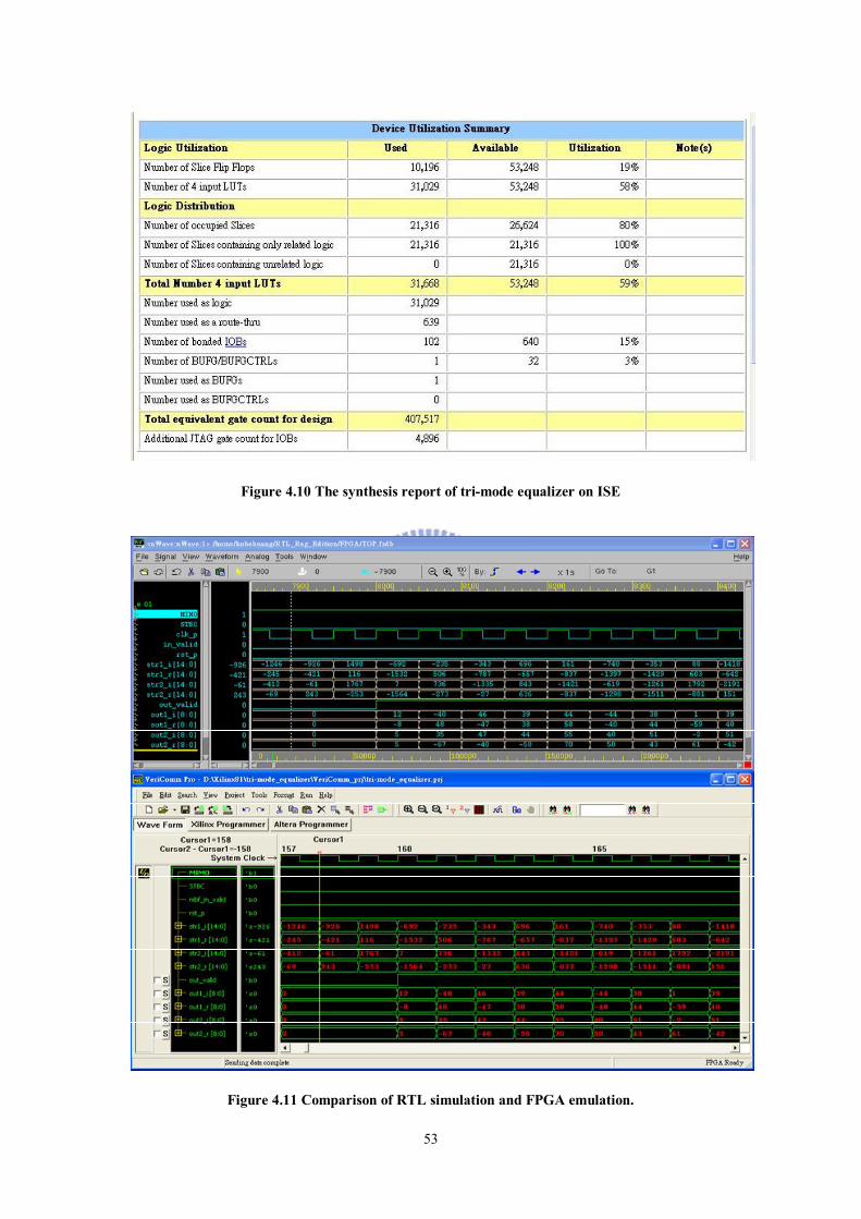
Figure 4.10 The synthesis report of tri-mode equalizer on ISE
Figure 4.11 Comparison of RTL simulation and FPGA emulation.

54
Figure 4.12 VeriComm and FPGA board
For FPGA verification, the tri-mode equalizer is also synthesized by XST
Synthesizer built in Xilinx ISE, the synthesis report is show as Fig 4.10.
Finally, to verify the functional correctness on FPGA, the comparisons of the
simulation results of RTL on nWave and emulation results of FPGA on VeriComm are
shown in Fig 4.11. Fig. 4.12 depicts the verifying situation. We claim that their
behaviors are correct from Fig 4.11 because the outputs are totally identical as
inputting the same patterns.

55
Chapter 5 Conclusions and Future Works
In this thesis, we proposed a tri-mode equalizer design which can operate in
SISO/SDM-MIMO/STBC-MIMO for IEEE 802.11n draft. The architecture of
tri-mode equalizer is divided to four portions: CFO mitigation, channel estimation,
phase error tracking and MIMO detection. In CFO mitigation, the proposed algorithm
increases the accuracy of channel estimation effectively and has low complexity in
hardware. Zero Forcing channel estimation for SISO mode can be fully integrated into
MIMO channel estimation for SDM-MIMO/STBC-MIMO modes in the proposed
architecture, so shared-architecture leads to low area consumption for tri-mode
channel estimator. In the proposed PET, a full tracking range can be achieved by the
pilot pre-compensation scheme, the performance degradation of conventional
pilot-based PET due to few pilot numbers can be improved outstandingly, and shared
architectures are also considered in the proposed circuit. Finally, Zero Forcing
equalization for SISO mode, MMSE MIMO symbol detection for SDM-MIMO mode
and ML MIMO symbol detection for STBC-MIMO mode are implemented with a lot
of shared architectures to reduce area consumption in circuit. Simulation results show
the proposed tri-mode equalizer achieves a better 1.9~3.8dB gain in SNR for 10%
PER compared with conventional approaches because a total solution of residual CFO
are proposed. In hardware implementation, totally 209k gate counts are used for
tri-mode equalizer. Low area consumption in the proposed circuit design is achieved
by using a lot of shared architectures.

56
In this thesis, we focus on equalizer design for 2x2 MIMO systems. Using this
design concept, a tri-mode inner receiver can also be considered in the future. For
higher data rate and higher reliability transmission, a MIMO system with higher
antenna dimensions will be certainly applied in the future. Therefore, an MIMO
equalizer in the high throughput transmission with more antennas will be needed to
further explore in the future.
57
Bibliography
[1] S. M. Alamouti, “A simple transmit diversity technique for wireless communications,” IEEE Journel on Select Areas in Communications, vol. 16, pp. 1451-1458, Oct. 1998.
[2] V. Tarokh, H. Jafarkhani, and A. R. Calderbank, “Space-time block codes from orthogonal designs,” IEEE Trans. Inform. Theory, vol. 45, pp. 1456–1467, July 1999.
[3] J. Liu and J. Li, “Parameter estimation and error reduction for OFDM-based WLANs,” IEEE Trans. Mobile Computing, vol 3, no 2, pp. 152-163, April-June 2004.
[4] F. Peng, and J. Zhan, “On Residual Carrier Frequency Offset Mitigation for 802.11N,” in Proc. ICASSP, 2007, vol. 3, p. 257-260.
[5] IEEE 802.11 TGn channel model special committee, “TGn Channel Models for IEEE 802.11 WLANs”, IEEE doc.: IEEE 802.11-03/940r4, May 2004.
[6] A. P. Stephens, “IEEE 802.11 TGn comparison criteria, Tech. Rep. IEEE 802.11-03/814r31, May 2004.
[7] A.A.M. Saleh and R.A. Valenzuela, “A statistical model for indoor multipath propagation,” IEEE J. Select. Areas Commun., vol. 5, 1987, pp. 128-137.
[8] Q.H. Spencer, et al., “Modeling the statistical time and angle of arrival characteristics of an indoor environment,” IEEE J. Select. Areas Commun., vol. 18, no. 3, March 2000, pp. 347-360.
[9] R.J-M. Cramer, R.A. Scholtz, and M.Z. Win, “Evaluation of an ultra-wide-band propagation channel,” IEEE Trans. Antennas Propagat., vol. 50, no.5, May 2002, pp. 561-570.
[10] Chia-Chin Chong, David I. Laurenson and Stephen McLaughlin, “Statistical Characterization of the 5.2 GHz wideband directional indoor propagation channels with clustering and correlation properties,” in proc. IEEE Veh. Technol.

58
Conf., vol. 1, Sept. 2002, pp. 629-633.
[11] L. Schumacher, K. I. Pedersen, and P.E. Mogensen, “From antenna spacings to theoretical capacities – guidelines for simulating MIMO systems,” in Proc. PIMRC Conf., vol. 2, Sept. 2002, pp. 587-592.
[12] L. Schumacher “WLAN MIMO Channel Matlab program,” download information: http://www.info.fundp.ac.be/~lsc/Research/IEEE_80211_HTSG_CMSC/distribution_terms.html
[13] IEEE 802.11 working group, IEEEP802.11n/D0.02, Feb 2006.
[14] Shou-Yin Liu, long-Wha Chong, “A study of joint tracking algorithms of carrier frequency offset and sampling clock offset for OFDM-based WLANs”, Communications, Circuit and System and West Sino Expositions. IEEE International Conference, vol. I, pp. 109-113, July. 2002.
[15] Wireless LAN Medium Access Control (MAC) and Physical Layer (PHY) Specifications: High Speed Physical Layer (PHY) in the 5 GHz Band, IEEE Standard 802.11a, 1999.
[16] Y.H. Yu, H.Y. Liu, T.Y. Hsu, and C.Y. Lee, “A Joint Scheme of Decision-Directed Channel Estimation and Weighted-Average Phase Error Tracking for OFDM WLAN Systems”, in Proc. APCCAS, 2004, vol. 2 , pp. 629-633
[17] P. Y. Tsai, H. Y. Kang, and T. D. Chiueh, “Joint weighted least squares estimation of frequency and timing offset for OFDM systems over fading channels,” in Proc. IEEE VTC’03, Cheju, Korea, Apr. 2003, pp. 2543–2547.
[18] A. V. Zeist "Space Division Multiplexing algorithms," 10th Mediter-ranean Electrotechnical Conference, vol.3, 2000.
[19] Joint Proposal Team PHY Simulation Results: IEEE 802.11-06/0067r02
[20] I-Tai Lu, Hsin-Chang Wu, Yongwen Yang, Olesen, R.,” Carrier Frequency Offset Mitigation in a Proposed MIMO OFDM System,” Systems, Applications and

59
Technology Conference, IEEE International Conference, pp. 1-5, May. 2007.
[21] Chia-Sheng Peng, Yuan-Shin Chuang, Kuei-Ann Wen,” CORDIC-based architecture with channel state information for OFDM baseband receiver,” IEEE Trans. Consumer Electronics, vol 51, pp. 403-412, May 2005.
[22] Shingo Yoshizawa and Yoshikazu Miyanaga, “VLSI implementation of high-throughput SISO-OFDM and MIMO-OFDM transceivers,” International Symposium on Communications and Information Technologies (ISCIT), No. T2D-4, Oct. 2006.
[23] Gilbert, J.M., Won-Joon Choi, Qinfang Sun, “MIMO technology for advanced wireless local area networks,” in Proc. Design Automation Conference, 2005, pp. 413-415
[24] Seongjoo Lee, Seungpyo Noh, Yunho Jung, Jaeseok Kim, “Efficient design of symbol detector for MIMO-OFDM based wireless LANs,” ICT-MICC, IEEE International Conference, pp. 510-514, May. 2007.
60
Vita 姓名 : 黃俊彥
性別 : 男
籍貫 : 宜蘭縣
生日 : 民國七十三年一月二十四日
地址 :宜蘭市西後街 131號
學歷 : 國立交通大學電子工程研究所碩士班 95/09~97/06
國立中興大學電機工程學系 91/09~95/06
國立宜蘭高級中學 88/09~91/06
論文題目 : A Tri-mode MIMO Equalizer Design for OFDM Based Wireless LANs
三模MIMO之無線區域網路等化器設計