Embed Size (px)
Citation preview

. . . . . .
Overview
• ガウス過程 (Gaussian Process)とは• 線形回帰から非線型回帰へ• ガウス過程の最適化とその問題• GPLVMとその最適化• GPDM• 最近のガウス過程研究
2 / 59

. . . . . .
ガウス過程 (Gaussian Process)とは
y
x−8 −6 −4 −2 0 2 4 6 8−3
−2
−1
0
1
2
• 入力 x → y を予測する回帰関数 (regressor)の確率モデル
− データ D ={(x(n), y(n))
}Nn=1が与えられた時,新しい
x(n+1) に対する y(n+1) を予測− ランダムな関数の確率分布− 連続空間で動く,ベイズ的なカーネルマシン (後で)
3 / 59

. . . . . .
ガウス過程 (Gaussian Process)とは
y
x−8 −6 −4 −2 0 2 4 6 8−4
−3
−2
−1
0
1
2
3
• 入力 x → y を予測する回帰関数 (regressor)の確率モデル
− データ D ={(x(n), y(n))
}Nn=1が与えられた時,新しい
x(n+1) に対する y(n+1) を予測− ランダムな関数の確率分布− 連続空間で動く,ベイズ的なカーネルマシン (後で)
3 / 59

. . . . . .
ガウス過程 (Gaussian Process)とは
y
x
• 入力 x → y を予測する回帰関数 (regressor)の確率モデル− データ D =
{(x(n), y(n))
}Nn=1が与えられた時,新しい
x(n+1) に対する y(n+1) を予測− ランダムな関数の確率分布− 連続空間で動く,ベイズ的なカーネルマシン (後で)
4 / 59

. . . . . .
線形モデル
y = w0 + w1x1 + w2x2 + ϵ
= (w0 w1 w2)︸ ︷︷ ︸wT
1
x1x2
︸ ︷︷ ︸x
+ϵ
= wTx+ ϵ
w = (XTX)−1XTy
(正規方程式)
• 簡単だが,直線的な関係しか表せない…「多変量解析」は今でもこれ
5 / 59

. . . . . .
一般化線形モデル (GLM)
y = w0 + w1x+ w2x2 + w3x
3 + ϵ (1)
= (w0 w1 w2 w3)︸ ︷︷ ︸wT
1
x
x2
x3
︸ ︷︷ ︸ϕ(x)
+ϵ (2)
= wTϕ(x) + ϵ (3)
• 非線型な関係を表せる• 基底関数 ϕ(x)が原点中心→もっと複雑にしたい!
6 / 59

. . . . . .
一般化線形モデル (GLM) (2)
−1 0 10
0.25
0.5
0.75
1
ϕ(x) =
(−(x− µ1)
2
2σ2, − (x− µ2)
2
2σ2, · · · ,−(x− µK)2
2σ2
)(4)
• 基底関数により,複雑な関数が作れる!− 基底関数のパラメータ µ = (µ1, µ2, · · · , µK)は固定・有限でよい? 7 / 59

. . . . . .
線形回帰モデル
• 入力 xから出力 y ∈ Rを予測する回帰関数 y = f(x)を求めたい
− x = (x1, · · · , xd) ∈ Rd は時間や任意のベクトル• y = f(x)を, xを一般の関数 ϕ(x)で変換した上で線形モデルで表してみる
y = wTϕ(x) (5)
例: ϕ(x) = (ϕ1(x), ϕ2(x), · · · , ϕH(x))T
= (1, x1, · · · , xd, x21, · · · , x2d)T
w = (w0, w1, · · · , w2d)T
のとき,
y = wTϕ(x)
= w0 + w1x1 + · · ·+ wdxd + wd+1x21 + · · ·+ w2dx
2d .
8 / 59

. . . . . .
GPの導入 (1)
• y(1) · · · y(N) について同時に書くと,下のように y = Φw と行列形式で書ける (Φ : 計画行列)
y(1)
y(2)
...y(N)
=
ϕ1(x
(1)) · · · ϕH(x(1))
ϕ1(x(2)) · · · ϕH(x(2))
......
ϕ1(x(N)) · · · ϕH(x(N))
w1
w2
...
...wH
(6)
y Φ w
• 重み w がガウス分布 p(w) = N(0, α−1I)に従っているとすると,y = Φw もガウス分布に従い,
• 平均 0,分散⟨yyT ⟩ =
⟨(Φw) (Φw)T
⟩= Φ⟨wwT ⟩ΦT (7)
= α−1ΦΦT の正規分布となる
9 / 59

. . . . . .
GPの導入 (2)
p(y) = N(y|0, α−1ΦΦT ) (8)
は,どんな入力 {xn}Nn=1 についても成り立つ→ガウス過程の定義• どんな入力 (x1,x2, · · · ,xN )についても,対応する出力y = (y1, y2, · · · , yN )がガウス分布に従うとき, p(y)はガウス過程に従う という.− ガウス過程 =無限次元のガウス分布− ガウス分布の周辺化はまたガウス分布なので,実際にはデータのある所だけの有限次元
• K = α−1ΦΦT の要素であるカーネル関数
k(x,x′) = α−1ϕ(x)Tϕ(x′) (9)
だけでガウス分布が定まる− k(x,x′)は xと x′の距離 ; 入力 xが近い→出力 y が近い
10 / 59

. . . . . .
GPの導入 (3)
• 実際には,観測値にはノイズ ϵが乗っている{y = wTϕ(x) + ϵ
ϵ ∼ N(0, β−1I)=⇒ p(y|f) = N(wTϕ(x), β−1I) (10)
• 途中の f = wTϕ(x)を積分消去
p(y|x) =∫
p(y|f)p(f |x)df (11)
= N(0,C) (12)
− 二つの独立なGaussianの畳み込みなので, Cの要素は共分散の和:
C(xi,xj) = k(xi,xj) + β−1δ(i, j). (13)
− GPは,カーネル関数 k(x,x′)とハイパーパラメータ α, β
だけで表すことができる.11 / 59

. . . . . .
様々なカーネル
−5 −4 −3 −2 −1 0 1 2 3 4 5−2.5
−2
−1.5
−1
−0.5
0
0.5
1
1.5
2
2.5
x
y
−5 −4 −3 −2 −1 0 1 2 3 4 5−3
−2
−1
0
1
2
3
x
y
Gaussian: exp(−(x− x′)2/l) Exponential: exp(−|x− x′|/l) (OU process)
−5 −4 −3 −2 −1 0 1 2 3 4 5−3
−2
−1
0
1
2
3
x
y
−5 −4 −3 −2 −1 0 1 2 3 4 5−2.5
−2
−1.5
−1
−0.5
0
0.5
1
1.5
2
2.5
x
y
Periodic: exp(−2 sin2(x−x′
2)/l2) Periodic(L): exp(−2 sin2(x−x′
2)/(10l)2)
12 / 59

. . . . . .
直観的理解
• Correlated Gaussian
K =
ガウス分布からのサンプル 分散・共分散行列
13 / 59
. . . . . .
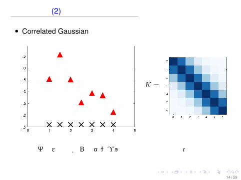
直観的理解 (2)
• Correlated Gaussian
K =
ガウス分布からのサンプル 分散・共分散行列
14 / 59

. . . . . .
直観的理解 (3)
• Correlated Gaussian
K =
ガウス分布からのサンプル 分散・共分散行列
15 / 59

. . . . . .
“Infinite” dimensional Gaussian
• もし,任意の (x1, x2, · · · , xn)について対応するy = (y1, y2, · · · , yn)がガウス分布に従うなら, yはガウス過程に従うという.
− 原理的には (x1, x2, · · · , xn)以外の次元もあるが,それらについて周辺化されている (←ガウス分布の周辺分布はガウス分布)
− 「無限次元」のガウス分布.• カーネル行列K の要素 Kij = k(xi, xj)を与えるカーネル kがガウス過程のパラメータ.
16 / 59

. . . . . .
「基底関数」の消去
• RBF基底関数 ϕ(x) = exp((x− h)2/r2)を考えてみる
• 1次元の場合, hを無限個用意すると
k(x,x′) = σ2H∑
h=1
ϕh(x)ϕh(x′) (14)
→∫ ∞
−∞exp
(−(x− h)2
r2
)exp
(−(x′ − h)2
r2
)dh (15)
=√πr2 exp
(−(x− x′)2
2r2
)≡ θ1 exp
(−(x− x′)2
θ22
)(16)
− (x,x′)のRBFカーネルは,無限個のRBF基底関数を考えたことと等価.
− カーネルのパラメータ θ1, θ2 は最尤推定で最適化できる
17 / 59

. . . . . .
GPの予測
• 新しい入力 ynew とこれまでの y の結合分布がまたGaussianになるので,
p(ynew|xnew,X,y, θ) (17)
=p((y, ynew)|(X,xnew), θ)
p(y|X, θ)(18)
∝ exp
−1
2([y, ynew]
[K k
kT k
]−1 [y
ynew
]− yTK−1y)
(19)
∼ N(kTK−1y, k − kTK−1k). (20)
ここで
− K = [k(x,x′)].− k = (k(xnew,x1), · · · , k(xnew,xN )).
18 / 59

. . . . . .
GP ↔ SVR, Ridge
• 機械翻訳の自動評価, ARDカーネル関数 (Cohn+ 2013)
k(x,x′) = σ2f exp
(−1
2
∑k
(xk − x′k)2
σ2k
)(21)
Model MAE RMSE
µ 0.8279 0.9899SVM 0.6889 0.8201
Linear ARD 0.7063 0.8480Squared exp. Isotropic 0.6813 0.8146
Squared exp. ARD 0.6680 0.8098Rational quadratic ARD 0.6773 0.8238
Matern(5,2) 0.6772 0.8124Neural network 0.6727 0.8103
Table 1: Single-task learning results on the
WMT12 dataset, trained and evaluated against
the weighted averaged response variable. µ is a
baseline which predicts the training mean, SVM
uses the same system as the WMT12 QE task, and
the remainder are GP regression models with dif-
ferent kernels (all include additive noise).
solution for a simpler model. For instance, mod-
els using ARD kernels were initialised from an
equivalent isotropic kernel (which ties all the hy-
perparameters together), and independent per-task
noise models were initialised from a single noise
model. This approach was more reliable than ran-
dom restarts in terms of accuracy and runtime ef-
ficiency.
Evaluation: We evaluate predictive accuracy
using two measures: mean absolute error,
MAE = 1
N
∑
N
i=1|yi − yi| and root mean square
error, RMSE =√
1
N
∑
N
i=1(yi − yi)
2, where yi
are the gold standard response values and yi are
the model predictions.
4.2 Results
Our experiments aim to demonstrate the efficacy
of GP regression, both the single task and multi-
task settings, compared to competitive baselines.
WMT12: Single task We start by comparing
GP regression with alternative approaches using
the WMT12 dataset on the standard task of pre-
dicting a weighted mean quality rating (as it was
done in the WMT12 QE shared task). Table 1
shows the results for baseline approaches and the
GP models, using a variety of different kernels
(see Rasmussen and Williams (2006) for details of
the kernel functions). From this we can see that all
models do much better than the mean baseline and
that most of the GP models have lower error than
the state-of-the-art SVM. In terms of kernels, the
linear kernel performs comparatively worse than
non-linear kernels. Overall the squared exponen-
Model MAE RMSE
µ 0.8541 1.0119Independent SVMs 0.7967 0.9673
EasyAdapt SVM 0.7655 0.9105
Independent 0.7061 0.8534Pooled 0.7252 0.8754
Pooled & {N} 0.7050 0.8497
Combined 0.6966 0.8448Combined & {N} 0.6975 0.8476
Combined+ 0.6975 0.8463Combined+ & {N} 0.7046 0.8595
Table 2: Results on the WMT12 dataset, trained
and evaluated over all three annotator’s judge-
ments. Shown above are the training mean base-
line µ, single-task learning approaches, and multi-
task learning models, with the columns showing
macro average error rates over all three response
values. All systems use a squared exponential
ARD kernel in a product with the named task-
kernel, and with added noise (per-task noise is de-
noted {N}, otherwise has shared noise).
tial ARD kernel has the best performance under
both measures of error, and for this reason we use
this kernel in our subsequent experiments.
WMT12: Multi-task We now turn to the multi-
task setting, where we seek to model each of the
three annotators’ predictions. Table 2 presents
the results. Note that here error rates are mea-
sured over all of the three annotators’ judgements,
and consequently are higher than those measured
against their average response in Table 1. For com-
parison, taking the predictions of the best model,
Combined, in Table 2 and evaluating its averaged
prediction has a MAE of 0.6588 vs. the averaged
gold standard, significantly outperforming the best
model in Table 1.
There are a number of important findings in Ta-
ble 2. First, the independently trained models do
well, outperforming the pooled model with fixed
noise, indicating that naively pooling the data is
counter-productive and that there are annotator-
specific biases. Including per-annotator noise to
the pooled model provides a boost in performance,
however the best results are obtained using the
Combined kernel which brings the strengths of
both the independent and pooled settings. There
are only minor differences between the different
multi-task kernels, and in this case per-annotator
noise made little difference. An explanation for
the contradictory findings about the importance
38
19 / 59

. . . . . .
GP ↔ SVR, Ridge
• 機械翻訳の自動評価, ARDカーネル関数 (Cohn+ 2013)
k(x,x′) = σ2f exp
(−1
2
∑k
(xk − x′k)2
σ2k
)(22)
Model MAE RMSE
µ 0.8279 0.9899SVM 0.6889 0.8201
Linear ARD 0.7063 0.8480Squared exp. Isotropic 0.6813 0.8146
Squared exp. ARD 0.6680 0.8098Rational quadratic ARD 0.6773 0.8238
Matern(5,2) 0.6772 0.8124Neural network 0.6727 0.8103
Table 1: Single-task learning results on the
WMT12 dataset, trained and evaluated against
the weighted averaged response variable. µ is a
baseline which predicts the training mean, SVM
uses the same system as the WMT12 QE task, and
the remainder are GP regression models with dif-
ferent kernels (all include additive noise).
solution for a simpler model. For instance, mod-
els using ARD kernels were initialised from an
equivalent isotropic kernel (which ties all the hy-
perparameters together), and independent per-task
noise models were initialised from a single noise
model. This approach was more reliable than ran-
dom restarts in terms of accuracy and runtime ef-
ficiency.
Evaluation: We evaluate predictive accuracy
using two measures: mean absolute error,
MAE = 1
N
∑
N
i=1|yi − yi| and root mean square
error, RMSE =√
1
N
∑
N
i=1(yi − yi)
2, where yi
are the gold standard response values and yi are
the model predictions.
4.2 Results
Our experiments aim to demonstrate the efficacy
of GP regression, both the single task and multi-
task settings, compared to competitive baselines.
WMT12: Single task We start by comparing
GP regression with alternative approaches using
the WMT12 dataset on the standard task of pre-
dicting a weighted mean quality rating (as it was
done in the WMT12 QE shared task). Table 1
shows the results for baseline approaches and the
GP models, using a variety of different kernels
(see Rasmussen and Williams (2006) for details of
the kernel functions). From this we can see that all
models do much better than the mean baseline and
that most of the GP models have lower error than
the state-of-the-art SVM. In terms of kernels, the
linear kernel performs comparatively worse than
non-linear kernels. Overall the squared exponen-
Model MAE RMSE
µ 0.8541 1.0119Independent SVMs 0.7967 0.9673
EasyAdapt SVM 0.7655 0.9105
Independent 0.7061 0.8534Pooled 0.7252 0.8754
Pooled & {N} 0.7050 0.8497
Combined 0.6966 0.8448Combined & {N} 0.6975 0.8476
Combined+ 0.6975 0.8463Combined+ & {N} 0.7046 0.8595
Table 2: Results on the WMT12 dataset, trained
and evaluated over all three annotator’s judge-
ments. Shown above are the training mean base-
line µ, single-task learning approaches, and multi-
task learning models, with the columns showing
macro average error rates over all three response
values. All systems use a squared exponential
ARD kernel in a product with the named task-
kernel, and with added noise (per-task noise is de-
noted {N}, otherwise has shared noise).
tial ARD kernel has the best performance under
both measures of error, and for this reason we use
this kernel in our subsequent experiments.
WMT12: Multi-task We now turn to the multi-
task setting, where we seek to model each of the
three annotators’ predictions. Table 2 presents
the results. Note that here error rates are mea-
sured over all of the three annotators’ judgements,
and consequently are higher than those measured
against their average response in Table 1. For com-
parison, taking the predictions of the best model,
Combined, in Table 2 and evaluating its averaged
prediction has a MAE of 0.6588 vs. the averaged
gold standard, significantly outperforming the best
model in Table 1.
There are a number of important findings in Ta-
ble 2. First, the independently trained models do
well, outperforming the pooled model with fixed
noise, indicating that naively pooling the data is
counter-productive and that there are annotator-
specific biases. Including per-annotator noise to
the pooled model provides a boost in performance,
however the best results are obtained using the
Combined kernel which brings the strengths of
both the independent and pooled settings. There
are only minor differences between the different
multi-task kernels, and in this case per-annotator
noise made little difference. An explanation for
the contradictory findings about the importance
38
20 / 59

. . . . . .
GP>SVRの利点
確率モデルなので,• ハイパーパラメータが第二種最尤推定で求められる• 予測の期待値だけでなく,分散も求まる
− 予測がどのくらい確かか/あやふやかがわかる• 複数の予測タスクを関係づけられる (Cohn+ 2014 etc.)• 性能が高い!
21 / 59

. . . . . .
GPの計算量
• GPの問題: 学習/推論時に X のグラム行列 K−1 を計算する必要…O(N3)の計算量
− N > 1000を超えると,実質的に計算不可能• 解決:「代表的」な仮想的なm個の入力 Xmを考え,もとの尤度を近似するようにXmを最適化→ O(m2N)の計算量
22 / 59

. . . . . .
ナイーブな方法
• Subset of Data : データの一部でカーネル行列を計算
K ≃ Kmm (23)
− データのうち,ランダムなm個のみによるカーネル行列− 計算量 O(m3)
• 単純にデータをほとんど捨てている→分散が大きく,低精度
23 / 59

. . . . . .
ナイーブな方法
• Subset of Data : データの一部でカーネル行列を計算
K ≃ Kmm (24)
− データのうち,ランダムなm個のみによるカーネル行列− 計算量 O(m3)
• 単純にデータをほとんど捨てている→分散が大きく,低精度
QUINONERO-CANDELA AND RASMUSSEN
!15 !10 !5 0 5 10 15!1.5
!1
!0.5
0
0.5
1
1.5
SoD
!15 !10 !5 0 5 10 15!1.5
!1
!0.5
0
0.5
1
1.5
SoR
!15 !10 !5 0 5 10 15!1.5
!1
!0.5
0
0.5
1
1.5
DTC
!15 !10 !5 0 5 10 15!1.5
!1
!0.5
0
0.5
1
1.5
ASoR/ADTC
!15 !10 !5 0 5 10 15!1.5
!1
!0.5
0
0.5
1
1.5
FITC
!15 !10 !5 0 5 10 15!1.5
!1
!0.5
0
0.5
1
1.5
PITC
Figure 5: Toy example with identical covariance function and hyperparameters. The squared ex-
ponential covariance function is used, and a slightly too short lengthscale is chosen on
purpose to emphasize the different behaviour of the predictive uncertainties. The dots
are the training points, the crosses are the targets corresponding to the inducing inputs,
randomly selected from the training set. The solid line is the mean of the predictive
distribution, and the dotted lines show the 95% confidence interval of the predictions.
Augmented DTC (ADTC) is equivalent to augmented SoR (ASoR), see Remark 12.
1952
24 / 59

. . . . . .
ナイーブな方法 (2)
• Subset of Regressors (Silverman 1985) :m個の基底でカーネル行列を近似
K ≃ KnmK−1mmKmn = K ′ (25)
− Knm : N ×mのグラム行列− 計算量 O(m2N)
25 / 59

. . . . . .
ナイーブな方法 (2)
• Subset of Regressors (Silverman 1985) :m個の基底でカーネル行列を近似
K ≃ KnmK−1mmKmn = K ′ (26)
− Knm : N ×mのグラム行列− 計算量 O(m2N)
• 目的関数に選んだ基底が含まれているため,過学習が起こる
QUINONERO-CANDELA AND RASMUSSEN
!15 !10 !5 0 5 10 15!1.5
!1
!0.5
0
0.5
1
1.5
SoD
!15 !10 !5 0 5 10 15!1.5
!1
!0.5
0
0.5
1
1.5
SoR
!15 !10 !5 0 5 10 15!1.5
!1
!0.5
0
0.5
1
1.5
DTC
!15 !10 !5 0 5 10 15!1.5
!1
!0.5
0
0.5
1
1.5
ASoR/ADTC
!15 !10 !5 0 5 10 15!1.5
!1
!0.5
0
0.5
1
1.5
FITC
!15 !10 !5 0 5 10 15!1.5
!1
!0.5
0
0.5
1
1.5
PITC
Figure 5: Toy example with identical covariance function and hyperparameters. The squared ex-
ponential covariance function is used, and a slightly too short lengthscale is chosen on
purpose to emphasize the different behaviour of the predictive uncertainties. The dots
are the training points, the crosses are the targets corresponding to the inducing inputs,
randomly selected from the training set. The solid line is the mean of the predictive
distribution, and the dotted lines show the 95% confidence interval of the predictions.
Augmented DTC (ADTC) is equivalent to augmented SoR (ASoR), see Remark 12.
1952
26 / 59

. . . . . .
ナイーブな方法の問題点
• カーネル行列 K を変更することで,モデル自体を書き換えている
− 真のモデルと違った事前分布による学習(Quinonero-Candela & Rasmussen 2005)
− 真の分布との「距離」が必要⇓
変分ベイズ法.
27 / 59

. . . . . .
変分近似 (Titsias 2009)
• 真の目的関数を変えてしまうのではなく,真の目的関数を下から近似する− Jensenの不等式:
log
∫p(x)f(x)dx ≥
∫p(x) log f(x)dx
• 入力 Xm に対応するGPの値を fm とおくと,
log p(y) = log
∫p(y, f , fm)dfdfm (27)
= log
∫q(f , fm)
p(y, f , fm)
q(f , fm)dfdfm (28)
≥∫
q(f , fm) logp(y, f , fm)
q(f , fm)dfdfm (29)
− ここで, q(f , fm)は下限を作るための補助分布28 / 59

. . . . . .
変分近似 (2)
• p(y, f , fm) = p(y|f)p(f |fm)p(fm)だから,
q(f , fm) = p(f |fm)q(fm)
とおけば,
log p(y) ≥∫
q(f , fm) logp(y, f , fm)
q(f , fm)dfdfm (30)
=
∫p(f |fm)q(fm) log
p(y|f)����p(f |fm)p(fm)
����p(f |fm)q(fm)dfdfm (31)
=
∫p(f |fm)q(fm) log
p(y|f)p(fm)
q(fm)dfdfm (32)
=
∫q(fm)
[∫p(f |fm) log p(y|f)df︸ ︷︷ ︸
G(fm)
+ logp(fm)
q(fm)
]dfm
(33)
29 / 59

. . . . . .
変分近似 (3)
• G(fm)を計算すると,
G(fm) =
∫p(f |fm) log p(y|f)df (34)
=
∫p(f |fm)
(−N
2log(2πσ2)− (y − f)2
2σ2
)df (35)
=
∫p(f |fm)
[−N
2log(2πσ2)− 1
2σ2tr(yT y−2yT f+fT f)
]df
(36)= −N
2log(2πσ2)
− 1
2σ2
[yT y−2yTα+αTα+tr
(Knn −KnmK−1
mmKmn
)](α = E[f |fm] = KnmK−1
mmfm)
(37)
= logN(y|α, σ2I)− 1
2σ2tr(Knn−K ′
nn
). (38)
30 / 59

. . . . . .
変分近似 (4)
• よって,
log p(y) ≥∫
q(fm)
[G(fm) + log
p(fm)
q(fm)
]dfm (39)
=
∫q(fm)
[log N(y|α, σ2I)− 1
2σ2tr(Knn−K ′
nn
)+ log
p(fm)
q(fm)
]dfm (40)
=
∫q(fm)
[log
N(y|α, σ2I)
q(fm)+ log p(fm)
]dfm
− 1
2σ2tr(Knn−K ′
nn) (41)
ここで Jensen boundを逆に使って,∫p(x) log
f(x)
p(x)dx ≤ log
∫f(x)dx (42)
31 / 59

. . . . . .
変分近似 (5)
• より,
下限 ≤ log
∫N(y|α, σ2I)p(fm)dfm − 1
2σ2tr(Knn −K ′
nn)
(K ′nn = KnmK−1
mmKmn) (43)
• α = E[f |fm] = KnmK−1mmfm を思い出すと,ガウス積分の公式から∫
N(y|α, σ2I)p(fm)dfm = N(y|0, σ2I +K ′nn) (44)
よって,下限は
log p(y) ≥ log N(y|0, σ2I +K ′nn)−
1
2σ2tr(Knn−K ′
nn) . (45)
32 / 59

. . . . . .
変分近似 (6)
• 変分下限の意味
log N(y|0, σ2I +K ′nn)−
1
2σ2tr(Knn−K ′
nn)
= logN(y|0, σ2I +K ′nn)−
1
2σ2tr(Cov(f |fm)) (46)
− 第 1項: fm によるデータへのフィット− 第 2項: fm による真のカーネル行列 Knn の近似度合い
• ナイーブな方法では,第 1項のみを最適化している.
33 / 59

. . . . . .
GPによる分類と SVM
• y = {+1,−1}のとき, p(y|f) = σ(y · f) (logit) or Ψ(y · f)(probit)で分類器になる
minimize: − log p(y|f)p(f |X)
=1
2fTK−1f −
N∑i=1
log p(yi|fi) (47)
• ソフトマージン SVMでは Kα = f とすると,
w =∑i
αixi → |w|2 = αTKα = fTK−1f ゆえ,
minimize:1
2|w|2 − C
N∑i=1
(1− yifi)+
=1
2fTK−1f − C
N∑i=1
(1− yifi)+ . (48)
− そっくりだが, SVMは hinge lossなのでスパース.34 / 59

. . . . . .
Loss functionsC. E. Rasmussen & C. K. I. Williams, Gaussian Processes for Machine Learning, the MIT Press, 2006,ISBN 026218253X. c© 2006 Massachusetts Institute of Technology. www.GaussianProcess.org/gpml
144 Relationships between GPs and Other Models
−2 0 1 4
0
1
2
log(1 + exp(−z))
−log Φ(z)
max(1−z, 0)
z
gǫ(z)
−ǫ 0 −ǫ.
(a) (b)
Figure 6.3: (a) A comparison of the hinge error, gλ and gΦ. (b) The ǫ-insensitiveerror function used in SVR.
For both the hard and soft margin SVM QP problems a wide variety ofalgorithms have been developed for their solution; see Scholkopf and Smola[2002, ch. 10] for details. Basic interior point methods involve inversions of n×n
matrices and thus scale asO(n3), as with Gaussian process prediction. However,there are other algorithms, such as the sequential minimal optimization (SMO)algorithm due to Platt [1999], which often have better scaling in practice.
Above we have described SVMs for the two-class (binary) classification prob-lem. There are many ways of generalizing SVMs to the multi-class problem,see Scholkopf and Smola [2002, sec. 7.6] for further details.
Comparing Support Vector and Gaussian Process Classifiers
For the soft margin classifier we obtain a solution of the form w =∑
i αixi
(with αi = λiyi) and thus |w|2 =∑
i,j αiαj(xi ·xj). Kernelizing this we obtain
|w|2 = α⊤Kα = f⊤K−1f , as5 Kα = f . Thus the soft margin objective
function can be written as
1
2f⊤K−1f + C
n∑
i=1
(1− yifi)+. (6.37)
For the binary GP classifier, to obtain the MAP value f of p(f |y) we minimizethe quantity
1
2f⊤K−1f −
n∑
i=1
log p(yi|fi), (6.38)
cf. eq. (3.12). (The final two terms in eq. (3.12) are constant if the kernel isfixed.)
For log-concave likelihoods (such as those derived from the logistic or pro-bit response functions) there is a strong similarity between the two optimiza-tion problems in that they are both convex. Let gλ(z) , log(1 + e−z), gΦ =
5Here the offset w0 has been absorbed into the kernel so it is not an explicit extra param-
eter.
• カーネル法でお馴染みの議論− SVMとMEの関係についても,同様な関係が成り立つ
• 注意: 分類したいだけなら, GP classifierは回りくどすぎる (他の理由があるなら有効)
35 / 59

. . . . . .
DPとの関係
• Gaussian processと Dirichlet processの定義はそっくり[偶然ではない]
− GP:どんな (x1,x2, · · · ,x∞)をとってきても,対応する(y1, y2, · · · , y∞)がガウス分布に従う
− DP:空間のどんな離散化 (X1, X2, · · · , X∞)についても,対応する離散分布がディリクレ分布Dir(α(X1), α(X2), · · · , α(X∞))に従う
• どちらも,無限次元の smootherになっている
36 / 59

ガウス過程の教師なし学習
. . . . . .

. . . . . .
確率的主成分分析
• Probabilistic PCA (Tipping & Bishop 1999){yn = Wxn + ϵ
ϵ ∼ N(0, σ2I)(49)
• よって,
L = log p(yn) = logN(Wxn, σ2I) (50)
= −N
2
(log 2π + log |C|+ tr(C−1S)
)(51)
ここで,
C = WWT + σ2I (52)
S =1
NYYT . (53)
38 / 59

. . . . . .
確率的主成分分析 (2)
• ∂L
∂W= 0より,尤度 Lを最大にするWの最尤推定値は
→ W ≡ Uq(Λq − σ2I)12 (σ2 = 0のとき UqΛ
12 ) (54)
− Λq, Uq : YYT の最大 q個の固有値・固有ベクトルを並べた行列
• σ2 = 0で通常の主成分分析と一致
39 / 59
. . . . . .
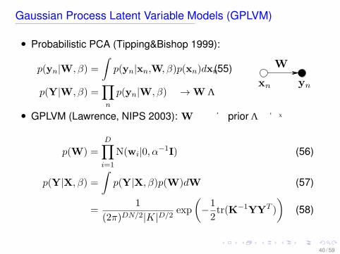
Gaussian Process Latent Variable Models (GPLVM)
• Probabilistic PCA (Tipping&Bishop 1999):
p(yn|W, β) =
∫p(yn|xn,W, β)p(xn)dxn(55)
p(Y|W, β) =∏n
p(yn|W, β) → Wを最適化
• GPLVM (Lawrence, NIPS 2003): W の方に priorを与えて積分消去
p(W) =
D∏i=1
N(wi|0, α−1I) (56)
p(Y|X, β) =
∫p(Y|X, β)p(W)dW (57)
=1
(2π)DN/2|K|D/2exp
(−1
2tr(K−1YYT )
)(58)
40 / 59

. . . . . .
GPLVM (2): PPCAのDual
log p(Y|X, β) = −DN
2log(2π)− D
2log |K| − 1
2tr(K−1YYT )
(59)K = αXXT + β−1I (60)
X = [x1, · · · ,xN ]T (61)
• Xに関して微分すると,∂L
∂X= αK−1YYTK−1X− αDK−1X = 0 (62)
⇐⇒ X =1
DYYTK−1X ⇒ X ≃ UQLV
T (63)
− UQ (N ×Q) : YYT の Q個の最大固有値 λ1 · · ·λQ に対応する固有ベクトル
− L = diag(l1, · · · , lQ); li = 1/√
λiαD − 1
αβ
41 / 59

. . . . . .
GPLVM (3) : Kernel化
log p(Y|X, β) = −DN
2log(2π)− D
2log |K| − 1
2tr(K−1YYT )
K = αXXT + β−1I , (64)
X = [x1, · · · ,xN ]T (65)
• 自然にカーネル化されている=⇒任意のカーネルKを導入
k(xn,xm) = α exp(−γ
2(xn − xm)2
)+ δ(n,m)β−1 (66)
• ∂L
∂K= K−1YYTK−1 −DK−1
− ∂L
∂xn,j=
∂L
∂K
∂K
∂xn,jを適用して微分
− Scaled Conjugate Gradientで解けるGPLVM in MATLAB: http://www.cs.man.ac.uk/˜neill/gplvm/
42 / 59

. . . . . .
GPLVM (4): 例
−0.8 −0.6 −0.4 −0.2 0 0.2 0.4 0.6−0.5
−0.4
−0.3
−0.2
−0.1
0
0.1
0.2
0.3
−0.2 −0.1 0 0.1 0.2 0.3
−0.25
−0.2
−0.15
−0.1
−0.05
0
0.05
0.1
0.15
0.2
0.4
0.6
0.8
1
1.2
1.4
1.6
1.8
2
2.2
2.4
Figure 1: Visualisation of the Oil data with (a) PCA (a linear GPLVM) and (b) A GPLVM whichuses an RBF kernel. Crosses, circles and plus signs represent stratifi ed, annular and homogeneousflows respectively. The greyscales in plot (b) indicate the precision with which the manifold wasexpressed in data-space for that latent point. The optimised parameters of the kernel were !"#$%&'( ,) "*(+, -.('/ and 0"*/+$12 .
2.2 A Practical Algorithm for GPLVMs
There are three main components to our revised, computationally efficient, optimisationprocess:
Sparsification. Kernel methods may be sped up through sparsification, i.e. representingthe data-set by a subset, 3 , of points known as the active set. The remainder, the inactiveset, is denoted by 4 . We make use of the informative vector machine [6] which selectspoints sequentially according to the reduction in the posterior process’s entropy that theyinduce.
Latent Variable Optimisation. A point from the inactive set, ! , can be shown to projectinto the data space as a Gaussian distribution
!"# $ " % & " ' # '() ' *+, $ % $ " % 5 " '6789" & ' (3)
whose mean is 5 " , ( T ) * -: ! :'; : ! " where ) : ! : denotes the kernel matrix developed fromthe active set and ; : ! " is a column vector consisting of the elements from the ! th column of) that correspond to the active set. The variance is 7 9" , " # & " ' & " * + ; T: ! " ) * -: ! : ; : ! " , Notethat since & " does not appear in the inverse, gradients with respect to & " do not depend onother data in 4 . We can therefore independently optimise the likelihood of each $ " withrespect to each & " . Thus the full set -<= can be optimised with one pass through the data.
Kernel Optimisation. The likelihood of the active set is given by
!.#.( : * , /#0123 * 4 5 % ) : ! : % 65 789:; < + /1 ( T: ) * -: ! : ( : = ' (4)
which can be optimised5 with respect to # , ) and
with gradient evaluations costing# % $ ' ,Algorithm 1 summarises the order in which we implemented these steps. Note that whilstwe never optimise points in the active set, we repeatedly reselect the active set so it is
5 In practice we looked for MAP solutions for all our optimisations, specifying a unit covarianceGaussian prior for the matrix > and using $?@ ) , $?@> and $?@% for ) , and respectively.
• 線形の PPCA(左)より, GP-LVM(右)の方が分離性能が高い− ベイズなので, Confidenceの分布が同時に得られる
• 計算量が問題 (O(N3)): active set (サポートベクターみたいなもの)を選んで,データをスパース化して最適化
43 / 59

. . . . . .
GPLVM (4): Caveat
• PCAではなく,ランダムに初期化した場合の結果
− Neil Lawrenceのコードで, 1e-2*randn(N,dims)で初期化
− Scaled conjugate gradientで最適化
−0.03 −0.02 −0.01 0 0.01 0.02 0.03−0.03
−0.02
−0.01
0
0.01
0.02
0.03
44 / 59

. . . . . .
GPLVM (5): 時系列データ
0 20 40 60 80 100−1.5
−1
−0.5
0
0.5
1
1.5
−1 −0.5 0 0.5 1−1
−0.8
−0.6
−0.4
−0.2
0
0.2
0.4
0.6
0.8
1
入力 正解
45 / 59

. . . . . .
GPLVM (6): 最適化結果
−1.5 −1 −0.5 0 0.5 1 1.5−1.5
−1
−0.5
0
0.5
1
1.5
計算結果
46 / 59

. . . . . .
GPLVM (6): 最適化結果
−1.5 −1 −0.5 0 0.5 1 1.5−1.5
−1
−0.5
0
0.5
1
1.5
−1.5 −1 −0.5 0 0.5 1 1.5−1.5
−1
−0.5
0
0.5
1
1.5
計算結果 PCAによる初期化
47 / 59

. . . . . .
GPLVM (7): MCMCによる計算
−1 −0.5 0 0.5 1
−1
−0.5
0
0.5
1
−4 −2 0 2 4 6−4
−3
−2
−1
0
1
2
3
4
Local Global
• MCMCで注意深く最適化 (ステップ=0.2, 400 iteration)• 点はすべて 0で初期化• 点を「繋ぐ」ような制約はない (→ GPDM)
48 / 59

. . . . . .
GPLVM (8): MCMCによる計算 (Oil Flow)
Local Global
• MCMCで計算すると, X にクラスタが現れる• ただし, X に外れ値が発生
49 / 59

. . . . . .
Gaussian Process Dynamical Model (Hertzmann 2005)
http://www.dgp.toronto.edu/˜jmwang/gpdm/
• GPLVMでは,潜在変数 xn に分布がなかった⇓
• xn が (GPで)時間発展するモデル.− 人間の動き (角度ベクトル)等の時系列データ.− 自然言語の時系列データ?
50 / 59

. . . . . .
GPDM (2): Formulation (1)
{xt = f(xt−1;A) + ϵx,t
yt = g(xt;B) + ϵy,t,
f ∼ GP(0,Kx) (67)
g ∼ GP(0,Ky) (68)
• 結合確率 p(Y,X|α, β) = p(Y|X, β)p(X|α)を考える.• 第 1項
p(Y|X, β) =|W|N
(2π)ND/2|KY |D/2exp
(−1
2tr(K−1
Y YW2YT )
)(69)
はGPLVMと基本的に同じ.− KY は (この論文では)普通の RBFカーネル
51 / 59

. . . . . .
GPDM (3): Formulation (2)
• 第 2項はMarkov時系列
p(X|α) = p(x1)
∫ N∏t=2
p(xt|xt−1,A, α) p(A|α)︸ ︷︷ ︸Gaussian
dA (70)
= p(x1)1
(2π)d(N−1)/2|KX |dexp
(−1
2tr(K−1
X X−XT−)
)(71)
− X− = [x2, · · · ,xN ]T とおいた− KX は x1 · · ·xN−1 の RBF+線形カーネル
k(x,x′) = α1 exp(−α2
2||x− x′||2
)+ α3x
Tx+ α−14 δ(x,x′) .
(72)
52 / 59

. . . . . .
GPDM (4): Formulation(3)
p(Y,X, α, β) = p(Y|X, β)p(X|α)p(α)p(β) (73)
p(α) ∝∏i
α−1i , p(β) ∝
∏i
β−1i . (74)
• 対数尤度は
− log p(Y,X, α, β) =1
2tr(K−1
X X−XT−) +
1
2tr(K−1
Y YW2YT )
+d
2log |KX |+ D
2log |KY | (正則化項)
− log |W|+∑j
logαj +∑j
log βj︸ ︷︷ ︸(定数)
(75)
−→最小化. (76)
53 / 59

. . . . . .
Gaussian Process Density Sampler (1)
−3 −2 −1 0 1 2 3−3
−2
−1
0
1
2
3
(a) ℓx =1, ℓy =1, α=1
−3 −2 −1 0 1 2 3−3
−2
−1
0
1
2
3
(b) ℓx =1, ℓy =1, α=10
−3 −2 −1 0 1 2 3−3
−2
−1
0
1
2
3
(c) ℓx =0.2, ℓy =0.2, α=5
−3 −2 −1 0 1 2 3−3
−2
−1
0
1
2
3
(d) ℓx =0.1, ℓy =2, α=5
Figure 1: Four samples from the GPDS prior are shown, with 200 data samples. The contour lines show the ap-proximate unnormalized densities. In each case the base measure is the zero-mean spherical Gaussian with unitvariance. The covariance function was the squared exponential: K(x, x′) = α exp(− 1
2
∑iℓ−2
i(xi − x′
i)2),
with parameters varied as labeled in each subplot. Φ(·) is the logistic function in these plots.
assume that these functions are together parameterized by a set of hyperparameters θ. Given thesetwo functions and their hyperparameters, for any finite subset of X with cardinality N there is amultivariate Gaussian distribution on R
N [4]. We will take the mean function to be zero.
Probability density functions must be everywhere nonnegative and must integrate to unity. We definea map from a function g(x) : X → R, x ∈ X , to a proper density f(x) via
f(x) =1
Zπ[g]Φ(g(x))π(x) (1)
where π(x) is an arbitrary base probability measure on X , and Φ(·) : R → (0, 1) is a nonnegativefunction with upper bound 1. We take Φ(·) to be a sigmoid, e.g. the logistic function or cumulativenormal distribution function. We use the bold notation g to refer to the function g(x) compactlyas a vector of (infinite) length, versus its value at a particular x. The normalization constant is afunctional of g(x):
Zπ[g] =
∫dx′ Φ(g(x′))π(x′). (2)
Through the map defined by Equation 1, a Gaussian process prior becomes a prior distribution overnormalized probability density functions on X . Figure 2 shows several sample densities from thisprior, along with sample data.
3 Generating exact samples from the prior
We can use rejection sampling to generate samples from a common density drawn from the theprior described in Section 2. A rejection sampler requires a proposal density that provides an upperbound for the unnormalized density of interest. In this case, the proposal density is π(x) and theunnormalized density of interest is Φ(g(x))π(x).
If g(x) were known, rejection sampling would proceed as follows: First generate proposals {xq}from the base measure π(x). The proposal xq would be accepted if a variate rq drawn uniformlyfrom (0, 1) was less than Φ(g(xq)). These samples would be exact in the sense that they were notbiased by the starting state of a finite Markov chain. However, in the GPDS, g(x) is not known: it isa random function drawn from a Gaussian process prior. We can nevertheless use rejection samplingby “discovering” g(x) as we proceed at just the places we need to know it, by sampling from theprior distribution of the latent function. As it is necessary only to know g(x) at the {xq} to acceptor reject these proposals, the samples are still exact. This retrospective sampling trick has beenused in a variety of other MCMC algorithms for infinite-dimensional models [5, 6]. The generativeprocedure is shown graphically in Figure 2.
In practice, we generate the samples sequentially, as in Algorithm 1, so that we may be assuredof having as many accepted samples as we require. In each loop, a proposal is drawn from thebase measure π(x) and the function g(x) is sampled from the Gaussian process at this proposedcoordinate, conditional on all the function values already sampled. We will call these data theconditioning set for the function g(x) and will denote the conditioning inputs X and the conditioning
2
• GPは任意の関数の prior→確率密度関数のモデルに使えないか?
p(x) =1
Z(f)Φ(f(x))π(x) (77)
− f(x) ∼ GP(x) ; π(x) : 事前分布− Φ(x) ∈ [0, 1] : シグモイド関数
• ex. Φ(x) = 1/(1 + exp(−x))54 / 59

. . . . . .
Gaussian Process Density Sampler (2)
p(x) =1
Z(f)Φ(f(x))π(x) (78)
• 生成プロセス: Rejection sampling
1. Draw x ∼ π(x).2. Draw r ∼ Uniform[0, 1].3. If r < Φ(g(x)) then accept x; else reject x
• AcceptされたN 個の観測データの背後に, rejectされたM 個のデータとその場所が存在 (隠れ変数)
− 分配関数 Z(f)は求まらないが, Φ(g(x))は求まる→MCMC!
− Infinite Mixtureとは別の確率密度のモデル化
55 / 59

. . . . . .
まとめ
• Gaussian process…連続的な関数のベイズモデル
− カーネル関数で定義される,無限次元のガウス分布− 基底関数の空間での線形モデルで,重みを積分消去したもの
• カーネル設計が重要− カーネルの違いにより,さまざまな振舞い− カーネルのパラメータは,確率モデルなのでデータから最適化できる
• 回帰問題だけでなく,教師なし学習にも使える (GPLVM, GPDM)• 計算量が課題→変分近似による効率的計算
56 / 59

. . . . . .
Literature
• “Gaussian Process Dynamical Models”. J. Wang, D. Fleet, andA. Hertzmann. NIPS 2005.http://www.dgp.toronto.edu/ jmwang/gpdm/
• “Gaussian Process Latent Variable Models for Visualization ofHigh Dimensional Data”. Neil D. Lawrence, NIPS 2003.
• “The Gaussian Process Density Sampler”. Ryan PrescottAdams, Iain Murray and David MacKay. NIPS 2008.
• “Archipelago: Nonparametric Bayesian Semi-SupervisedLearning”. Ryan Prescott Adams and Zoubin Ghahramani.ICML 2009.
57 / 59

. . . . . .
参考文献・教科書
• 「パターン認識と機械学習」(Pattern Recognition and MachineLearning), Chapter 6. Christopher Bishop, Springer, 2006.http://ibisforest.org/index.php?PRML
• “Gaussian Processes for Machine Learning”. Rasmussen andWilliams, MIT Press, 2006.http://www.gaussianprocess.org/gpml/
• “Gaussian Processes — A Replacement for SupervisedNeural Networks?”. David MacKay, Lecture notes at NIPS1997. http://www.inference.phy.cam.ac.uk/mackay/GP/
− Videolectures.net: “Gaussian Process Basics”.http://videolectures.net/gpip06 mackay gpb/
• ガウス過程に関するメモ (1). 正田備也, 2007.http://www.iris.dti.ne.jp/˜tmasada/2007071101.pdf
58 / 59

. . . . . .
Codes
• GPML Toolbox (in MATLAB):http://www.gaussianprocess.org/gpml/code/
• GPy (in Python):http://sheffieldml.github.io/GPy/
59 / 59