國 立 交 通 大 學

電信工程研究所

碩 士 論 文

前瞻長程演進異質性網路的

頻譜與能源效率之分析

Investigation of Spectral and Energy Efficiency in LTE-A Heterogeneous Networks

研究生：謝宗展

指導教授：王蒞君

中 華 民 國 一百零一 年 六 月

前瞻長程演進異質性網路的

頻譜與能源效率之分析

Investigation of Spectral and Energy Efficiency in LTE-A Heterogeneous Networks

研 究 生：謝宗展 Student：Tsung-Chan Hsieh

指導教授：王蒞君 Advisor：Li-Chun Wang

國 立 交 通 大 學 電信工程研究所 碩 士 論 文

A Thesis

Submitted to Institute of Communications Engineering

College of Electrical and Computer Engineering

National Chiao Tung University

in partial Fulfillment of the Requirements

for the Degree of

Master of Science

In

Communication Engineering June 2012

Hsinchu, Taiwan, Republic of China

中華民國 一百零一 年 六 月

前瞻長程演進異質性網路的

頻譜與能源效率之分析

學生：謝宗展 指導教授：王蒞君 教授

國立交通大學

電機學院電信工程研究所

摘要

在此篇論文中，我們探討應用階層式基地台合作技術之第三代合

作夥伴前瞻長程演進異質性網路系統的頻譜與能源效率。我們發現同

時考慮系統架構與合作傳輸方法的設計能夠達到綠能傳輸之目的。因

為基地台合作之技術可以有效降低共同通道干擾與改善接收訊號品

質，且系統架構對於系統之表現有相當的影響。特別是考慮了同時結

合細胞間與細胞內基地台合作之方法。這篇論文呈現了利用上述之聯

合設計方法於應用階層式基地台合作技術之異質性網路系統表現的

改善。模擬結果顯示，採用我們提出的聯合設計方法之異質性網路系

統比起傳統單用戶多輸入多輸出系統是一個有效提高頻譜與能源效

率的方法。

Investigation of Spectral and Energy Efficiency

in LTE-A Heterogeneous Networks

A THESIS Presented to

The Academic Faculty By

Tsung-Chan Hsieh

In Partial Fulfillment

of the Requirements for the Degree of

Master in Communication Engineering

Institute of Communications Engineering

College of Electrical and Computer Engineering

National Chiao-Tung University

June, 2012

Copyright c⃝2012 by Tsung-Chan Hsieh

Abstract

In this thesis, we investigate both spectral and energy efficiency of hierarchical base

station cooperation techniques in heterogeneous networks (HetNet) of the 3rd Gener-

ation Partnership Project (3GPP) Long Term Evolution-Advanced (LTE-A) system.

We find that joint consideration of system architectures and cooperation schemes

will achieve energy-efficient transmission. Because the co-channel interference can be

mitigated significantly and the signal quality is able to be improved through base

station coordination techniques, and system architectures have great impacts on the

system performance. Especially, coordinated multi-point (CoMP) techniques of dif-

ferent levels, e.g., intra and inter-site CoMP, are considered jointly. We address the

performance improvements of HetNet system with hierarchical base station coordi-

nation techniques by the joint design of both system architecture and coordinated

transmission scheme. The proposed joint design methodology is a promising solution

for improving spectral and energy efficiency compared to the conventional single user

multi-input-multi-output (SU-MIMO) system.

Acknowledgments

Foremost, I would like to appreciate Professor Li-Chun Wang who has guided me for

more than three years. As the lyric goes, I once was lost, but now I am found. I

was so unfamiliar with what the true research is, but I have increased some more

understanding now.

Secondly, I want to thank all my laboratory members in Mobile Communications

and Cloud Computing Laboratory at the Institute of Communications Engineering

in National Chiao-Tung University. It is they that provide me so much assistance to

finish my research. Especially, Tsung-Ting Chiang spent a lot of his free time helping

me solve many problems.

Finally, I owe an enormously debt of gratitude to my parents for their great

support these years.

II

III

Contents

Abstract I

Acknowledgements II

List of Tables VI

List of Figures VII

1 Introduction 1

1.1 Motivation . . . . . . . . . . . . . . . . . . . . . . . . . . . . . . . . . 2

1.2 Issues . . . . . . . . . . . . . . . . . . . . . . . . . . . . . . . . . . . 2

1.3 Thesis Outline . . . . . . . . . . . . . . . . . . . . . . . . . . . . . . . 4

2 Background 5

2.1 Why Green Communication? . . . . . . . . . . . . . . . . . . . . . . . 5

2.2 Coordinated Multi-point Techniques . . . . . . . . . . . . . . . . . . 6

2.3 Literature Survey . . . . . . . . . . . . . . . . . . . . . . . . . . . . . 8

3 System Models 10

3.1 Cell Layout . . . . . . . . . . . . . . . . . . . . . . . . . . . . . . . . 10

3.1.1 Homogeneous Network SU-MIMO System . . . . . . . . . . . 10

3.1.2 Heterogeneous Network CoMP System . . . . . . . . . . . . . 12

3.2 Channel Model . . . . . . . . . . . . . . . . . . . . . . . . . . . . . . 14

3.2.1 Radio Environment . . . . . . . . . . . . . . . . . . . . . . . . 14

3.2.2 Sptial Channel Model . . . . . . . . . . . . . . . . . . . . . . . 15

3.3 Power Consumption Model Description . . . . . . . . . . . . . . . . . 17

3.3.1 Network Power Consumption . . . . . . . . . . . . . . . . . . 17

3.3.2 Base Station Power Consumption . . . . . . . . . . . . . . . . 18

4 Heterogeneous CoMP Networks Simulator 22

4.1 Codebook-based Precoding . . . . . . . . . . . . . . . . . . . . . . . . 22

4.2 Transmission Equations . . . . . . . . . . . . . . . . . . . . . . . . . 25

4.2.1 Single UE Case . . . . . . . . . . . . . . . . . . . . . . . . . . 26

4.2.2 Multiple UE Case . . . . . . . . . . . . . . . . . . . . . . . . . 28

4.3 CoMP Schemes . . . . . . . . . . . . . . . . . . . . . . . . . . . . . . 29

4.4 Proportional Fair Scheduling . . . . . . . . . . . . . . . . . . . . . . . 30

4.5 Exponential Effective SINR Mapping (EESM) . . . . . . . . . . . . . 32

4.6 Hybrid Automatic Repeat Request (HARQ) . . . . . . . . . . . . . . 32

4.7 Energy Efficiency . . . . . . . . . . . . . . . . . . . . . . . . . . . . . 33

5 Tradeoff Design of Spectral and Energy Efficiency in HetNet Sys-

tems 34

5.1 System Architectures . . . . . . . . . . . . . . . . . . . . . . . . . . . 34

5.2 CoMP Transmission Techniques . . . . . . . . . . . . . . . . . . . . . 35

5.3 Design Procedures . . . . . . . . . . . . . . . . . . . . . . . . . . . . 38

6 Numerical Results 40

6.1 Simulation Assumptions . . . . . . . . . . . . . . . . . . . . . . . . . 40

6.2 Simulation Baseline . . . . . . . . . . . . . . . . . . . . . . . . . . . . 40

6.3 Intra-site CoMP . . . . . . . . . . . . . . . . . . . . . . . . . . . . . . 42

6.3.1 Effect of RRH Deployment . . . . . . . . . . . . . . . . . . . . 42

6.3.2 Effect of Cell Architecture . . . . . . . . . . . . . . . . . . . . 45

6.3.3 Tradeoff between Spectral and Energy Efficiency . . . . . . . . 45

6.4 Inter plus Intra-site CoMP . . . . . . . . . . . . . . . . . . . . . . . . 49

IV

6.5 Reference Signal Received Power-Based RRH Selection . . . . . . . . 53

7 Conclusions 55

7.1 Thesis Summary . . . . . . . . . . . . . . . . . . . . . . . . . . . . . 55

7.2 Suggestions for Future Research . . . . . . . . . . . . . . . . . . . . . 56

Bibliography 57

Vita 60

V

VI

List of Tables

2.1 Comparison of Our Work and Related Works . . . . . . . . . . 9

3.1 Deployment regulations . . . . . . . . . . . . . . . . . . . . . . . . 12

3.2 Components of the site power . . . . . . . . . . . . . . . . . . . . 17

3.3 Power consumption for various BSs . . . . . . . . . . . . . . . . 21

4.1 Codebook for Two Antenna Ports . . . . . . . . . . . . . . . . . 23

4.2 Codebook for Four Antenna Ports . . . . . . . . . . . . . . . . . 24

6.1 Simulation Parameters . . . . . . . . . . . . . . . . . . . . . . . . 41

6.2 2x2 SU-MIMO Simulation Results Comparison . . . . . . . . . 42

6.3 Relative gains of intra-site CoMP schemes . . . . . . . . . . . . 48

VII

List of Figures

1.1 The relation between EE and SE. . . . . . . . . . . . . . . . . . . . . 4

2.1 Various CoMP scenarios. . . . . . . . . . . . . . . . . . . . . . . . . . 7

3.1 Cell architecture of SU-MIMO systems. . . . . . . . . . . . . . . . . . 11

3.2 Cell architecture of CoMP systems. . . . . . . . . . . . . . . . . . . . 13

3.3 Parameters of 3GPP SCM. . . . . . . . . . . . . . . . . . . . . . . . . 15

3.4 BBU+RRU based system. . . . . . . . . . . . . . . . . . . . . . . . . 19

3.5 Power model of a BS. . . . . . . . . . . . . . . . . . . . . . . . . . . . 20

4.1 Two cell scenario of CS/CB. . . . . . . . . . . . . . . . . . . . . . . . 31

5.1 Sector antenna architectures. . . . . . . . . . . . . . . . . . . . . . . . 36

5.2 Two kinds of CoMP schemes. . . . . . . . . . . . . . . . . . . . . . . 37

5.3 Joint design procedure for energy-efficient transmission. . . . . . . . . 39

6.1 Comparison of spectral efficiency for different RRH locations. . . . . . 44

6.2 Comparison of energy efficiency for different RRH locations. . . . . . 44

6.3 Comparison of spectral efficiency for different system architectures. . 46

6.4 Comparison of energy efficiency for different system architectures. . . 46

6.5 Tradeoff between spectral efficiency and energy efficiency of the intra-

site CoMP scheme. . . . . . . . . . . . . . . . . . . . . . . . . . . . . 47

6.6 Spectral efficiency comparison of different transmission schemes. . . . 49

6.7 Comparison of spectral efficiency for different transmission schemes in

the single UE case. . . . . . . . . . . . . . . . . . . . . . . . . . . . . 51

6.8 Comparison of energy efficiency for different transmission schemes in

the single UE case. . . . . . . . . . . . . . . . . . . . . . . . . . . . . 51

6.9 Comparison of spectral efficiency for different transmission schemes in

the multiple UE case. . . . . . . . . . . . . . . . . . . . . . . . . . . . 52

6.10 Comparison of energy efficiency for different transmission schemes in

the multiple UE case. . . . . . . . . . . . . . . . . . . . . . . . . . . . 52

6.11 Comparison of spectral efficiency for different RRH density with selection. 54

6.12 Comparison of energy efficiency for different RRH density with selection. 54

VIII

0

1

CHAPTER 1

Introduction

Due to the explosive growth in information and communication traffic as well as

demands of better quality of service (QoS) from subscribers, it is estimated that the

information and communication technology (ICT) energy consumption is rising at 15-

20 percentages per year, in other words, doubling every five years, and such striking

increase does not seem to slow down soon. It is reckoned that the ICT industry

is responsible for 3 percent of the worldwide annual electrical energy consumption,

causing 2-4 percent of world’s carbon dioxide emissions [1] [2]. With the increasing

awareness of gradual depletion of non-renewable resources and harmful environmental

impacts caused by carbon dioxide, it is the social responsibility that cellular network

operators should be devoted to develop energy-efficient telecommunication systems.

Aside from environmental aspects, the energy cost accounts a great portion of network

operators’ overall expenditure, and the electric bill is more than $10 billion dollars per

year [3]. At present, almost 80 percentages of electrical power for system operation

is attributed to radio access network (RAN) [4]. Therefore, efficient transmission

schemes and network architectures benefit not only ecological but also economical

aspects. Such improvements can be fulfilled in two ways: optimizing base stations

(BSs) via more efficient and traffic load adaptive modules, and innovating radio access

point deployment strategies as well as transmission technologies to lower the energy

consumption and achieve the required system performance.

1.1 Motivation

The traditional network system design mainly focused on spectral efficiency (SE).

Energy efficiency (EE) only received little attention, and seldom deemed as a vital

performance indicator. As energy-saving issue becomes more crucial, green communi-

cation gets more and more important. Therefore, not only SE but also EE should be

considered in the system design. There are several techniques to increasing the system

throughput. First of all, deploying small cells with macro-cells to build a heteroge-

neous network (HetNet), which is able to enhance received signal power to guarantee

acceptable signal to interference plus noise ratio (SINR). Secondly, higher data rate

can be rendered through coordinated multi-point (CoMP) techniques which allow

BSs to process signals jointly for mitigating interference [5] [6]. It is true that CoMP

and HetNet are promising techniques to improve the system capacity [7]. However,

it comes with a price: additional energy consumption. Because increasing BSs needs

more power consumption accordingly, and additional backhaul connections among

cooperating nodes as well as signal processing power to perform CoMP schemes also

need more energy. As mentioned above, both spectral and energy efficiency are vi-

tal performance indicators. Hence, the objective of this thesis is to assess spectral

and energy efficiency of CoMP transmission in HetNet systems, and to find the ap-

propriate transmission scheme and deployment strategy to achieve energy-efficient

transmission.

1.2 Issues

To address the characteristic of the relation between those two performance met-

rics [8], we consider a point-to-point transmission in additive white Gaussian noise

(AWGN) channel. In accordance with Shannon’s capacity equation, given the system

2

bandwidth W and the transmit power P , the maximal reliable transmission rate is

R =W log2(1 +P

WN0

), (1.1)

where N0 denotes the noise power spectral density. According to SE and EE defini-

tions, SE and EE are

ηSE =R

W= log2(1 +

P

WN0

), (1.2)

and

ηEE =R

P=W

Plog2(1 +

P

WN0

) (1.3)

respectively. From (1.2) and (1.3), we can get

2ηSE = 1 +P

WN0

. (1.4)

Then, the SE-EE relation can be expressed as

ηEE =ηSE

(2ηSE − 1)N0

, (1.5)

which is plotted in Fig. 1.1. From (1.5), as ηEE approaches to zero, ηSE tends to

infinity. In contrast, when ηEE approaches to zero, ηSE converges to 1/(N0 ln 2). It

is impossible to satisfy both metrics in the same time.

However, (1.5) is specific to point to point instead of networks transmission.

If more practical constrains and transmission strategies are taken into consideration,

such as transmission techniques, modulation and coding schemes, transmission dis-

tances, and resource allocation algorithms, the SE-EE curve will not be as monotonic

as shown in Fig 1.1 [9]. Therefore, it is worthy of assessing the SE-EE relation for

the future energy-efficient communication system design.

3

Figure 1.1: The relation between EE and SE.

1.3 Thesis Outline

The remainder of the thesis is organized as follows. In Chapter 2 we introduce the

background of our work. System models are illustrated in Chapter 3. In chapter

4, we address our simulation methodology of heterogeneous network CoMP systems.

The procedure of our joint design is described in Chapter 5. Then, the numerical and

simulation results are shown in Chapter 6. Finally, Chapter 7 concludes the thesis.

4

5

CHAPTER 2

Background

2.1 Why Green Communication?

The way people access information has been revolutionized by the consecutively re-

newing technology. Dramatic growth on data traffic and the requirements for ubiq-

uitous access have triggered tremendous expansion of network infrastructure and

correspondingly ascending escalation of energy needs. The estimated growing rate

of network subscribers is 20 percent per year, i.e., doubled every five years. It is

reckoned that the ICT industry is accountable for three percent of world’s annual

electrical power consumption and two to four percent of worldwide carbon dioxide

emission which put great threats on global environment. There have been shown that

about three billion mobile handsets and around three million base sites worldwide.

The electricity bill is more than 10 billion dollars each year [10]. From the oper-

ators’ perspective, reducing energy consumption not only diminishes carbon print,

but also saves operating expenditure costs, so the social responsibility and operation

profit are both catered. In fact, over 80 percent of the total ICT energy consump-

tion is attributed to the radio access network. Studies have clearly indicated that

the power drain of mobile handset equipments is far lower than that of BSs. Hence,

energy reduction schemes are supposed to mainly focus on BSs. Such a goal can be

achieved by renovating existing network structures with more energy efficient deploy-

ment strategies or applying novel transmission techniques of BSs. Briefly speaking,

energy-efficient technologies will be indispensable for helping ICT industries face chal-

lenges in a more and more energy-constrained future.

2.2 Coordinated Multi-point Techniques

Cooperation among BSs for data transmissions to one or more user equipment (UE)

is known as a key technique to reach the requirement of the IMT-Advance in terms

of both overall and cell-edge system throughput of cellular communication networks.

The network multiple-input-multiple-output (MIMO) technique is also referred as

CoMP by 3GPP. Moreover, it is thought to be one of potential contributors in en-

hancing energy efficiency of upcoming LTE-A systems. There are four downlink

CoMP deployment scenarios [11]:

(1) Scenario 1: Homogeneous network with intra-site CoMP, as shown in Fig. 2.1(a).

(2) Scenario 2: Homogeneous network with high transmit power remote radio heads

(RRHs). RRHs are linked to the macro-cell with high speed backhaul, as shown

in Fig. 2.1(b).

(3) Scenario 3: Heterogeneous network with low power RRHs within the macro-cell

coverage. RRHs share different cell IDs with the macro-cell, as shown in Fig.

2.1(c).

(4) Scenario 4: Heterogeneous network with low power RRHs within the macro-cell

coverage. RRHs share the same cell ID with the macro-cell, as shown in Fig.

2.1(c).

Although Scenarios 1 and 2 are developed the earliest, scenario 4 has the most

potential and advantages.

6

Macro cell

Coordination area

(a) Scenario1.

Macro cell

High Tx power RRH

Optical fiber

Coordination area

(b) Scenario2.

Macro cell

Low Tx power RRH

Optical fiber

Coordination area

(c) Scenario3/4.

Figure 2.1: Various CoMP scenarios.

7

In general, CoMP techniques can be categorized into two classes, which are

joint processing (JP) and coordinated scheduling / coordinated beamforming (CS/CB).

Most of current researches on CoMP schemes have focused on JP. In the class of JP,

by sharing channel state information among BSs through network backhaul, the sig-

nal can be processed jointly before transmitting and signals from other cells may

assist the communication instead of being treated as a detrimental interference. The

same information to the target UE is simultaneously transmitted from different co-

operating BSs through the same frequency resource and coherently or non-coherently

combined at the receiver side, which improves received signal quality and mitigates

interferences. In terms of CS/CB, the data to single UE is only available at and trans-

mitted from one point in the cooperating set for a time frequency resource, while user

scheduling/beamforming decisions are made among coordinated cells.

2.3 Literature Survey

HetNet is thought to be power efficient for deploying low power nodes to extend the

cell coverage and improve system capacity. It is true that SE may increase with the

denser network. However, both [12] and [13] indicated that as the number of pico

cells exceeds a certain amount, the gain in system throughput cannot compensate

the extra power consumption of pico sites, which degrades EE. Hence, small cell

deployment is suggested being limited under a certain degree. The work [14] further

analyzed HetNet in terms of EE and success probability, indicating that there exists

an optimal pico-macro density ratio that maximizes EE, which offers the knowledge

in how to establish green heterogeneous networks. [15] pointed out that despite that

overall EE is improved, but the macro-cell performance is slightly degraded due to

interferences from small cells. In brief, increasing small cells is not always beneficial

for improving the system throughput.

8

Table 2.1: Comparison of Our Work and Related Works

Heterogeneous Coordinated System SE-EE

Networks Multi-Point Architecture Analysis

[17] ×√ √ √

[16] ×√ √

×[18]

√ √× ×

[14]√

×√

×[15]

√×

√ √

Our Work√ √ √ √

CoMP techniques can improve network throughput significantly, but it also

requires more power to sustain such operations. In [16], authors compared system

capacity of various density cooperative networks. Their results shows the denser

network is, the SE higher will be. Nevertheless, the relation of energy efficiency is

not drawn. Tradeoff between cell throughput gains via inter-site CoMP scheme and

increased power dissipation has been investigated under various cell dimensions and

cooperation cluster sizes [17]. A similar investigation has been conducted in [18].

The energy efficiency analysis of joint transmission (JT) CoMP in homogeneous and

heterogeneous network is addressed. However, both [17] and [18] did not take the

concept of cooperation among macro-cell and lower power sites into consideration.

We analyze the system capacity and power consumption of heterogeneous CoMP

networks under various system settings to seek energy-efficient transmission schemes

and system architectures. Related researches are summarized and compared with our

work at Table 2.1.

9

10

CHAPTER 3

System Models

In this chapter, we illustrate our system models thoroughly. At the beginning, we

present the system architecture of our simulator, including the homogeneous network

for single user multi-input-multi-output (SU-MIMO) systems and the heterogeneous

network for CoMP systems. Channel model and radio environment are introduced in

the second section. The power consumption model is given in the last section.

3.1 Cell Layout

3.1.1 Homogeneous Network SU-MIMO System

MIMO transmission techniques have been studied extensively in the past. Spatial

multiplexing has drawn much attention due to the capability of increasing spectral

efficiency. Spatial multiplexing of multiple data streams to single target UE in the

same time-frequency resource is referred as SU-MIMO. We set the homogeneous net-

work SU-MIMO system composed by 19 cells with hexagonal gird as our simulation

baseline, which is shown in Fig. 3.1. Each cell is divided into three sectors, and each

sector is equipped with a directional antenna.

R

UE

Macrocell

Signal from macrocell

Figure 3.1: Cell architecture of SU-MIMO systems.

11

3.1.2 Heterogeneous Network CoMP System

In accordance with 3GPP-A Rel-11, downlink CoMP techniques can be categorized

into four scenarios, among of which scenario 4 is the most promising. We choose

scenario 4 as the simulation environment so as to combine the concepts of HetNet and

CoMP techniques. The cellular system is composed of 19 hexagonal cells, where each

cell is divided into 3 sectors, and every sector is equipped with directional antennas

as shown in Fig. 3.2. The benefit of using directional antenna is that the signal

can be concentrated to be transmitted within some range, which makes the signal

more strengthened and interferences among sectors can be mitigated. RRHs are

deployed in each sector and connected with the macro-cell by 109 bytes level optical

fibers. Fibers are able to carry a large amount of data. In this way, remote units can

exchange information with the macro-cell, and the signal processing can be jointly

performed by RRHs and the macro-cell in a centralized manner. Minimum distances

between the BS an UE are listed in Table 3.1.

Table 3.1: Deployment regulations

Minimum Distance

Macro-RRH > 75m

RRH-RRH > 40m

Macro-UE > 35m

RRH-UE > 10m

12

R

UE

RRH

Signal from macrocell

Signal from RRH

Backhaul

Macro cell

Figure 3.2: Cell architecture of CoMP systems.

13

3.2 Channel Model

3.2.1 Radio Environment

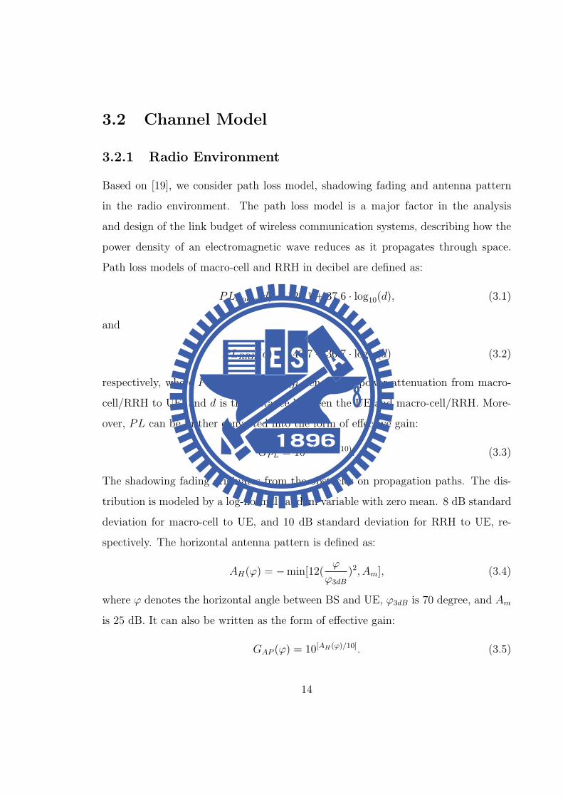
Based on [19], we consider path loss model, shadowing fading and antenna pattern

in the radio environment. The path loss model is a major factor in the analysis

and design of the link budget of wireless communication systems, describing how the

power density of an electromagnetic wave reduces as it propagates through space.

Path loss models of macro-cell and RRH in decibel are defined as:

PLmacro(d) = 128.1 + 37.6 · log10(d), (3.1)

and

PLRRH(d) = 140.7 + 36.7 · log10(d) (3.2)

respectively, where PLmacro and PLRRH denote the power attenuation from macro-

cell/RRH to UE, and d is the distance between the UE and macro-cell/RRH. More-

over, PL can be further converted into the form of effective gain:

GPL = 10−(PL(d)/10). (3.3)

The shadowing fading originates from the obstacles on propagation paths. The dis-

tribution is modeled by a log-normal random variable with zero mean. 8 dB standard

deviation for macro-cell to UE, and 10 dB standard deviation for RRH to UE, re-

spectively. The horizontal antenna pattern is defined as:

AH(φ) = −min[12(φ

φ3dB

)2, Am], (3.4)

where φ denotes the horizontal angle between BS and UE, φ3dB is 70 degree, and Am

is 25 dB. It can also be written as the form of effective gain:

GAP (φ) = 10[AH(φ)/10]. (3.5)

14

3.2.2 Sptial Channel Model

The Spatial channel model (SCM) is a standardized model developed by 3GPP for

evaluating cellular MIMO systems. In our work, we adopt SCM urban scenario [20].

Assume that there are N resolvable paths in each link from a BS to a UE, and each

path consists of M irresolvable subpaths. A simplified plot of SCM is shown in Fig.

3.3.

BSW

UEW

, ,n m AoDD

,n AoDd

,n AoAd, ,n m AoD

q

, ,n m AoAq

BSq

UEq

Vq, ,n m AoA

D

Figure 3.3: Parameters of 3GPP SCM.

For Nt transmit antennas at the BS and Nr receive antennas at the UE, the

channel impulse response in time domain for the nth path between the sth transmit

and uth receive antenna can be written as:

hn(t) =

h1,1,n(t) h1,2,n(t) · · · h1,Nt−1,n(t) h1,Nt,n(t)

h2,1,n(t) h2,2,n(t) · · · h2,Nt−1,n(t) h2,Nt,n(t)...

... · · · ......

hNr−1,1,n(t) hNr−1,2,n(t) · · · ......

hNr,1,n(t) hNr,2,n(t) · · · hNr,Nt−1,n(t) hNr,Nt,n(t)

. (3.6)

15

Each element in hn(t) can be written as:

hu,s,n(t) =

√PnM

M∑m=1

[ejkds sin(θn,m,AoD+ψn,m)ejkdu sin(θn,m,AoA)ejkV cos(θn,m,AoA−θV )t]. (3.7)

where Pn is the power of the nth path,M is the number of subpaths per path, k is the

carrier wave number which equals to 2π/λ, λ is the carrier wavelength in meters, ds

is the distance in meters from the first antenna to the sth antenna at the BS, θn,m,AoD

is the angle between the mth subpath of the nth path and the BS array broadside,

ψn,m is the phase of the mth subpath of the nth path which uniformly distributes in

the interval [0◦, 360◦], du is the distance in meters from the first antenna to the uth

antenna at the UE, θn,m,AoA is the angle between the mth subpath of the nth path

and the UE array broadside, V is the UE velocity, and θV is the angle between the

UE travel direction and the UE array broadside. For multi-carrier OFDM systems,

the channel impulse response from the sth transmit to the uth receive antenna in

frequency domain of the kth subcarrier is:

HSCM(k) =

H1,1(k) H1,2(k) · · · H1,Nt−1(k) H1,Nt(k)

H2,1(k) H2,2(k) · · · H2,Nt−1(k) H2,Nt(k)...

... · · · ......

HNr−1,1(k) HNr−1,2(k) · · · ......

HNr,1(k) HNr,2(k) · · · HNr,Nt−1(k) HNr,Nt(k)

. (3.8)

Each element in HSCM(k) can be expressed as:

Hu,s(k) = FFT{[hu,s,1(t), hu,s,2(t), ..., hu,s,n(t)]}, (3.9)

where FFT{·} denotes the Fourier transform function.

16

3.3 Power Consumption Model Description

3.3.1 Network Power Consumption

The total network input power includes power consumption in RAN, backhaul, and

signal processing for CoMP:

Ptotal = Psite + Psp + Pbh, (3.10)

where

Psite = PPDS + PAC + PTrans + PBS. (3.11)

Related details of Psite are listed in Table 3.2 [21]. Psp denotes the signal processing

power for cooperation, it can be expressed as [17]:

Psp = 58 · (0.87 + 0.1 ·Nc + 0.03 ·N2c ), (3.12)

where Nc denotes the number of cooperated sites. Pbh is the power for backhaul

connection, which can be written as:

Pbh =R

100M· 50, (3.13)

where R denotes the data rate.

Table 3.2: Components of the site power

Watt

PPDS 485.23

PAC 1940.96

PTrans 650

17

3.3.2 Base Station Power Consumption

There are different types of BS such as macro-cell, micro-cell, pico-cell, femto-cell, and

RRH. Because each kind of BS has different constituents and power figures, it is not

easy to describe the precise BS architectures and corresponding power dissipation

models thoroughly. In our work, we adopt the power consumption model of the

baseband unit (BBU) plus remote radio unit (RRU) based BS as illustrated in Fig.

3.4 [22]. The basic idea of BBU plus RRU system is to separate the baseband part and

the radio frequency part of BSs. RRUs are connected to the BBU with optical fibers,

and each RRU is equipped with transceivers. The BBU is responsible for baseband

signal processing and radio resource management, so the signal can be processed

jointly at BBUs. It is cost-saving for radio access points deployment because smaller

BBUs require less equipment room, and RRUs can be deployed more flexibly depends

on traffic needs.

Each BS consists of multiple transceivers (TRXs), and each TRX is comprised

of a power amplifier (PA), a radio frequency (RF) module, a baseband processor, a

DC-DC supply, and an AC-DC unit (mains supply), which is shown in Fig. 3.5. As

a result, we can decompose the power consumption model into four classes generally

[23] [24] :

(1) Power Amplifier (PA): In this part, we consider the PA power efficiency and feeder

losses which is caused by extra feedback for pre-distortion and additional signal

processing. For small cells, feeder losses are elided, but necessary in macro and

micro cells. The power consumption of a PA can be written as:

PPA =Pout

ηPA(1− σfeed), (3.14)

where ηPA is the PA efficiency, and σfeed is the feeder loss factor.

(2) Radio Frequency (RF): The RF part contains a transmitter and a receiver for

18

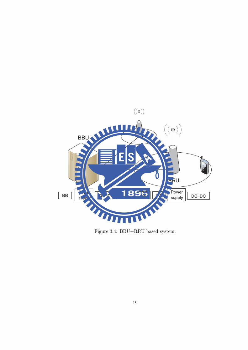
Figure 3.4: BBU+RRU based system.

19

Figure 3.5: Power model of a BS.

downlink and uplink, respectively. Different types of RF modules are required for

different types of BSs. For example, low-intermediate frequency (IF) are suitable

for macro and micro sites, and zero-IF is favored by smaller cells.

(3) Baseband unit: The baseband unit deals with modulation/demodulation, channel

coding/decoding, channel estimation, equalization, pre-distortion, etc.

(4) Heat emission: Any losses related to the system powering are included in this

category, such as DC-DC conversion and mains supply.

According to above, given PA, RF, and baseband unit power consumption,

PPA, PRF and PBB, the power consumption for BS input is:

PBS = β[NTRX(PPA + PRF + PBB)], (3.15)

where β is defined as:

β =1

(1− σDC)(1− σMS), (3.16)

and σDC , σMS,and σcool are loss factors of the DC/DC, mains supply and cooling

system. Thus, the input power for BS can be further expressed as:

PBS = NTRX ·Pmax

ηPA+ PRF + PBB

(1− σDC)(1− σMS). (3.17)

20

We assume that the BS power consumption is proportional to the number of transceiver

chains NTRX , namely, transmit/receive antenna pairs per site, and all the BSs with

the maximal load,

Pmax = 10(Pout+σfeed−30)/10. (3.18)

The related power consumption parameters of different types BSs are listed in Table

3.3.

Table 3.3: Power consumption for various BSs

Macro BBU Macro RRU Pico BBU Pico RRU

Pout [W] 0 46 0 30

σfeeder [dBm] 0 1 0 0

PA Pmax [W] 0 50.11 0 1

ηPA [%] 0 31.1 0 6.7

PPA [W] 0 161.15 0 14.92

Heat σDC [%] 8 8 9 9

emission σMS [%] 9 9 12 12

β # 1.19 1.19 1.24 1.24

RF PRF [W] 0 12.9 0 1

BB PBB [W] 29.6 0 3 0

Sectors # 3 1 1 1

Antennas # 2 2 1 1

Carriers # 1 1 1 1

Pin [W] 212.13 415.79 3.74 19.88

21

22

CHAPTER 4

Heterogeneous CoMP Networks Simulator

In this chapter, the simulation environment of the 3GPP LTE-A heterogeneous co-

ordination multi-point networks will be illustrated in details, including joint signal

process for base station cooperation, precoding method, scheduling method, and SINR

calculation.

4.1 Codebook-based Precoding

In FDD systems, the CSI needs to be fed back from UEs to the eNB. It is well

known that the system performance can be improved with full channel state infor-

mation (CSI) at the transmitter. However, because the feedback channel bandwidth

is limited, complete channel state feedback leads to excessive overhead. Therefore,

the codebook-based precoding method is adopted to reduce the feedback overhead.

The UE calculates the precoding matrix and feedback a precoding matrix indicator

(PMI) as the index of a codeword. The codebook is designed in the off-line manner,

and the same codebook set is available at both the transmitter and the receiver. The

feedback overhead can be reduced enormously by only feeding the PMI back rather

than the full precoding matrix.

Codebooks for two antenna and four transmit antenna ports are defined in [25].

Tables 4.1 and 4.2 list codewords for two and four transmit antenna ports, respectively.

The Frobenius norm of each codeword is normalized to unity to remain the same

transmit power.

Table 4.1: Codebook for Two Antenna Ports

Index Rank-1 Rank-2

C01√2

1

1

12

1 1

1 −1

C1

1√2

1

−1

12

1 1

j −j

C2

1√2

1

j

C3

1√2

1

−j

For four transmit antennas, the householder matrix Wc can be derived by uc,

i.e., Wc = I4 − 2ucuHc

/uHc uc. Wa

c denotes the ath column vector of Wc, and Wa,bc

denotes ath and bth column vectors of Wc.

We assume that UEs can estimate the CSI perfectly based on reference signals

from BSs. Singular value decomposition-based (SVD) precoding method is adopted

in our work. Denote Hm,n,i as the channel matrix from the mth sector to the ith UE

in the nth sector. Then, the channel matrix is decomposed by the SVD technique:

Hm,n,i = Um,n,iDm,n,iVHm,n,i, (4.1)

where

Um,n,i = [u1m,n,i · · · · · ·uNr

m,n,i] ∈ CNr×Nr , (4.2)

23

Table 4.2: Codebook for Four Antenna Ports

Index uc Rank-1 Rank-2

C0 u0 =

[1 −1 −1 −1

]TW1

0 W1,40

/√2

C1 u1 =

[1 −j 1 j

]TW1

1 W1,41

/√2

C2 u2 =

[1 1 −1 1

]TW1

2 W1,42

/√2

C3 u3 =

[1 j 1 −j

]TW1

3 W1,23

/√2

C4 u4 =

[1 (−1− j)

/√2 −j (1− j)

/√2

]TW1

4 W1,44

/√2

C5 u5 =

[1 (1− j)

/√2 j (1− j)

/√2

]TW1

5 W1,45

/√2

C6 u6 =

[1 (1 + j)

/√2 −j (−1 + j)

/√2

]TW1

6 W1,36

/√2

C7 u7 =

[1 (−1 + j)

/√2 j (1 + j)

/√2

]TW1

7 W1,37

/√2

C8 u8 =

[1 −1 1 1

]TW1

8 W1,28

/√2

C9 u9 =

[1 −j −1 −j

]TW1

9 W1,49

/√2

C10 u10 =

[1 1 1 −1

]TW1

10 W1,310

/√2

C11 u11 =

[1 j −1 j

]TW1

11 W1,311

/√2

C12 u12 =

[1 −1 −1 1

]TW1

12 W1,212

/√2

C13 u13 =

[1 −1 1 1−

]TW1

13 W1,313

/√2

C14 u14 =

[1 1 −1 −1

]TW1

14 W1,314

/√2

C15 u15 =

[1 1 1 1

]TW1

15 W1,215

/√2

24

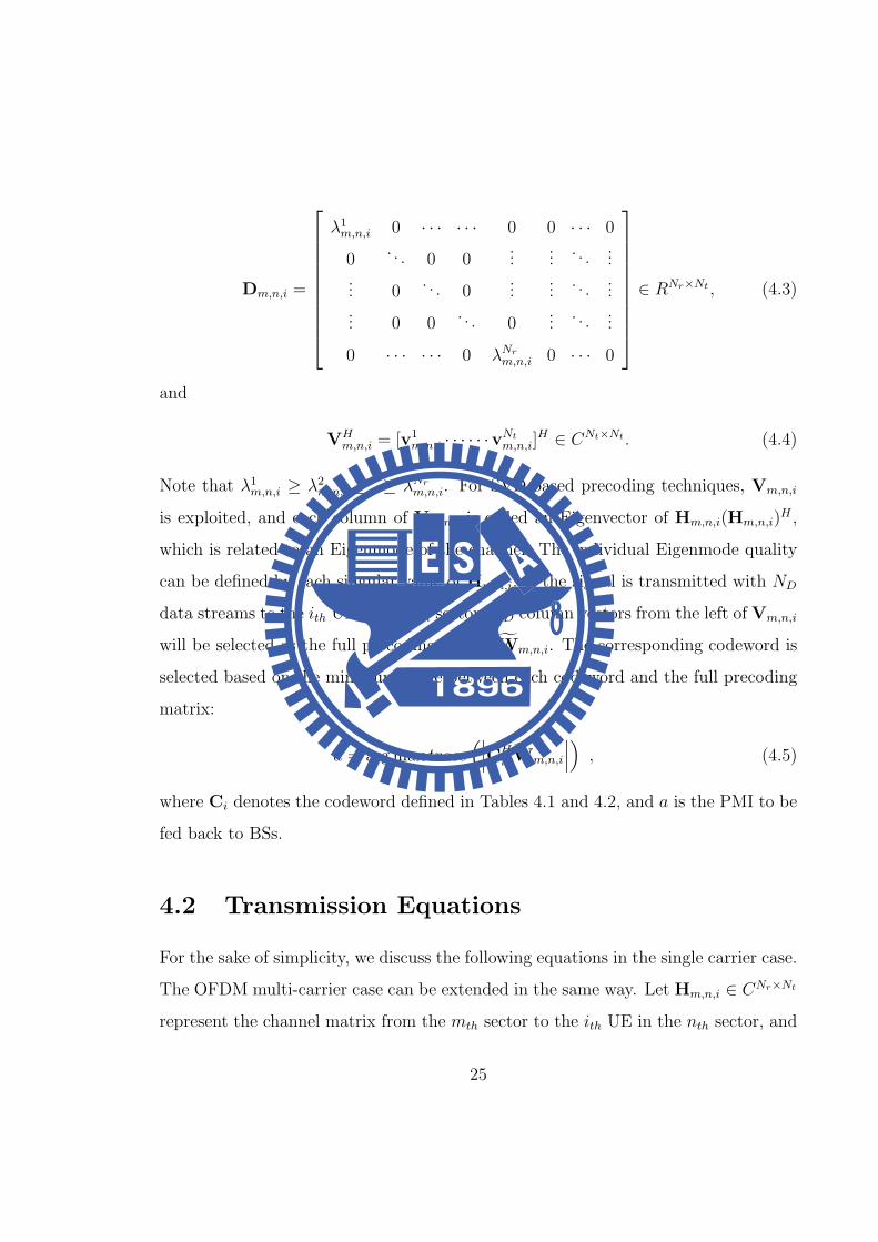
Dm,n,i =

λ1m,n,i 0 · · · · · · 0 0 · · · 0

0. . . 0 0

......

. . ....

... 0. . . 0

......

. . ....

... 0 0. . . 0

.... . .

...

0 · · · · · · 0 λNrm,n,i 0 · · · 0

∈ RNr×Nt , (4.3)

and

VHm,n,i = [v1

m,n,i · · · · · ·vNtm,n,i]

H ∈ CNt×Nt . (4.4)

Note that λ1m,n,i ≥ λ2m,n,i ≥...≥ λNrm,n,i. For SVD-based precoding techniques, Vm,n,i

is exploited, and each column of Vm,n,i is called an Eigenvector of Hm,n,i(Hm,n,i)H ,

which is related to an Eigenmode of the channel. The individual Eigenmode quality

can be defined by each singular value of Hm,n,i. If the signal is transmitted with ND

data streams to the ith UE in the nth sector, ND column vectors from the left of Vm,n,i

will be selected as the full precoding matrix W̃m,n,i. The corresponding codeword is

selected based on the minimum angle between each codeword and the full precoding

matrix:

a = argmaxitrace

(∣∣∣CHi W̃m,n,i

∣∣∣) , (4.5)

where Ci denotes the codeword defined in Tables 4.1 and 4.2, and a is the PMI to be

fed back to BSs.

4.2 Transmission Equations

For the sake of simplicity, we discuss the following equations in the single carrier case.

The OFDM multi-carrier case can be extended in the same way. Let Hm,n,i ∈ CNr×Nt

represent the channel matrix from the mth sector to the ith UE in the nth sector, and

25

HRRHmr,n,i ∈ CNr×Nt denotes the channel matrix from the rth RRH in the mth sector to

the ith UE in the nth sector similarly. In accordance with (3.3), (3.5), and (3.9), the

channel matrix Hm,n,i can be written as:

Hm,n,i = HSCM

√GPL · σS ·GAP , (4.6)

where σS is the shadowing factor. In the same manner, HRRHmr,n,i has a similar math-

ematic form with Hm,n,i. For SU-MIMO transmission, the effective channel matrix

Heffm,n,i ∈ CNr×Nt detected by the ith UE is

Heffm,n,i = Hm,n,i. (4.7)

As for CoMP transmission, RRHs share the same cell ID with the macro-cell, the

whole network can be regarded as a distributed antenna system. Thus data trans-

mitted by the macro-cell and RRHs are placed on the same resource blocks (RBs).

Consequently, the effective channel matrix Heffm,n,i ∈ CNr×Nt detected by the ith UE in

the nth sector is the combination of channel matrices from the macro-cell and RRHs,

which can be written as:

Heffm,n,i =

∑m

Hm,n,i +∑r

HRRHmr,n,i. (4.8)

4.2.1 Single UE Case

Assume that the nth sector is the serving sector antenna of the ith UE. The received

signal matrix of the ith UE in the nth sector can be written as:

Yn,n,i =

Desired signal︷ ︸︸ ︷Heffn,n,iWn,n,iXn,n,i+

Inter−cell interference︷ ︸︸ ︷57∑m̸=n

Heffm,n,iWm,m,iXm,m,i+

Noise︷ ︸︸ ︷Nn,n,i . (4.9)

The second term in (4.9) is the interference from other sectors. Thus Xn,n,i is the

desired data matrix to the ith UE in the nth sector, Wn,n,i is the precoding matrix to

26

the ith UE in the nth sector, and Nn,n,i ∈ CNr×1 is the additive white Gaussian noise

with power spectral density σ2n = −174dBm/Hz.

For the rank-1 transmission, the maximal ratio combining (MRC) technique is

adopted. Assume that the desired data matrix is Xn,n,i = x1n,n,i and the correspond-

ing precoding matrix is Wn,n,i = w1n,n,i. The desired data can be demodulated via

multiplying Yn,n,i by the MRC matrix:

Mn,n,i = [Heffn,n,iWn,n,i]

H . (4.10)

For the rank-2 transmission, the minimum mean square error (MMSE) receive tech-

nique is adopted. Assume that the desired data matrix is Xn,n,i =[x1n,n,i x2n,n,i

]and the corresponding precoding matrix is Wn,n,i =

[w1n,n,i w2

n,n,i

]. The desired

data can be demodulated via multiplying Yn,n,i by MMSE matrices M1n,n,i ∈ C1×Nr

and M2n,n,i ∈ C1×Nr , respectively, where

M1n,n,i =

[(σ2nI+Hn,n,iw

2n,n,i

(Hn,n,iw

2n,n,i

)H)−1

Hn,n,iw1n,n,i

]H, (4.11)

and

M2n,n,i =

[(σ2nI+Hn,n,iw

1n,n,i

(Hn,n,iw

1n,n,i

)H)−1

Hn,n,iw2n,n,i

]H. (4.12)

Hence, the received SINR of the ith UE in the nth sector can be written as:

γn,n,i =PTx

∥∥∥Mn,n,iHeffn,n,iWn,n,iXn,n,i

∥∥∥2

PTx

∥∥∥∥∥Mn,n,i

57∑m̸=n

Heffm,n,iWm,m,iXm,m,i

∥∥∥∥∥2

+ ∥Mn,n,iNn,n,i∥2, (4.13)

where PTx is the transmit power of BS.

27

4.2.2 Multiple UE Case

We assume that there are two UEs in each sector: the ith UE and the jth UE. The

received signal matrix of the ith UE in the nth sector can be written as:

Yn,n,i =

Desired signal︷ ︸︸ ︷Heffn,n,iWn,n,iXn,n,i+

Inter−user interference︷ ︸︸ ︷Heffn,n,jWn,n,jXn,n,j

+

Inter−cell interference︷ ︸︸ ︷57∑m̸=n

(Heffm,n,iWm,m,iXm,m,i +Heff

m,n,jWm,m,jXm,m,j)+

Noise︷ ︸︸ ︷Nn,n,i

. (4.14)

The second term of (4.14) is the interference from the other UE in the same cell,

and the third term is the interference from other cells. Likewise, we can derive the

received signal matrix of the jth UE in the nth sector like (4.14) in the same manner:

Yn,n,j =

Desired signal︷ ︸︸ ︷Heffn,n,jWn,n,jXn,n,j +

Inter−user interference︷ ︸︸ ︷Heffn,n,iWn,n,iXn,n,i

+

Inter−cell interference︷ ︸︸ ︷57∑m̸=n

(Heffm,n,jWm,m,jXm,m,j +Heff

m,n,iWm,m,iXm,m,i)+

Noise︷ ︸︸ ︷Nn,n,j

. (4.15)

To demodulate received signals of the ith and the jth UE, we multiply Yn,n,i

and Yn,n,j by MMSE matrix

M1n,n,i = [(σn

2I +Heffn,n,iWn,n,j(H

effn,n,iWm,m,j)

H)−1Heffn,n,iWn,n,i]

H (4.16)

and

M1n,n,j = [(σn

2I +Heffn,n,jWn,n,i(H

effn,n,jWm,m,i)

H)−1Heffn,n,jWn,n,j]

H , (4.17)

respectively. Hence, the received SINRs of the ith UE and the jth UE in the nth sector

can be written as:

γn,n,i =PTx

∥∥∥Mn,n,iHeffn,n,iWn,n,iXn,n,i

∥∥∥2

PTx

∥∥∥∥∥Mn,n,i

57∑m̸=n

Heffm,n,iWm,m,iXm,m,i

∥∥∥∥∥2

+ ∥Mn,n,iNn,n,i∥2, (4.18)

28

and

γn,n,j =PTx

∥∥∥Mn,n,jHeffn,n,jWn,n,jXn,n,j

∥∥∥2

PTx

∥∥∥∥∥Mn,n,j

57∑m̸=n

Heffm,n,jWm,m,jXm,m,j

∥∥∥∥∥2

+ ∥Mn,n,jNn,n,j∥2, (4.19)

respectively, where PTx is the transmit power of a BS.

4.3 CoMP Schemes

In the JP transmission, the precoding matrix is decided by decomposing the received

effective channel matrix from multiple BSs based on the SVD method. For the intra-

site JP, the effective channel matrix of the ith UE in the nth sector can be expressed

as

Heffm,n,i = Hm,n,i +

∑r

HRRHmr,n,i. (4.20)

For the inter-site plus intra-site JP, the effective channel matrix of the ith UE in the

nth sector can be expressed as

Heffm,n,i =

3∑m=1

Hm,n,i +∑r

HRRHmr,n,i. (4.21)

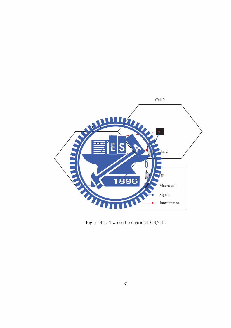
Apart from JP, we also consider the CS/CB technique for the inter-cell coor-

dination. All the three cells serve an UE in the same time for JP transmission. On

the other hand, each cell serves only an UE at a time, but manages to reduce the

interference to UEs in other cells for CS/CB transmission . Take a two cell system

as shown in Fig. 4.1 for illustration. We can express the received signal of UE1 as

Y1 = H11W1X1 +H21W2X2 +N, (4.22)

29

where H11 denotes the channel matrix from BS1 to UE1, H21 denotes the channel

matrix from BS2 to UE1. W1 and W2 are precoding matrices of UE1 and UE2,

respectively. The SINR of UE1 can be written as:

SINR1 =P1∥M1H11W1∥2

P2∥M1H21W2∥2 + σn2, (4.23)

where M denotes the demodulation matrix, P is the transmit power, and σn2 denotes

the thermal noise power. In order to maximize SINR1, the interference term of

(4.23) should be mitigated. Thus, once W1 is determined, we try to select a W2

which makes H21W2 approaches zero from the codebook, in other words, finding a

precoing matrix which tends to be orthogonal to the channel matrix. For the rank-1

transmission, W2 is chosen from the codebook according to

argminj(|H11W1(H21Wj)|H). (4.24)

For the rank-2 transmission, W2 is chosen from the codebook according to

argminj[tr(|H11W1(H21Wj)|H)]. (4.25)

4.4 Proportional Fair Scheduling

Proportional fair scheduling is a compromise-based scheduling algorithm. Both fair-

ness of all UEs and maximizing the network throughput are taken into account. If

maximizing network throughput is the highest priority, UEs with better link quality

will be always served and UEs with poor link quality will be neglected. With pro-

portional fair scheduling, both transmission rate and fairness are concerned. An UE

will be served if its current transmission rate is high or its past average transmission

rate is low. On the contrary, if the current transmission rate of another UE is low or

its past average transmission rate is high, its serving priority is lower than the former

30

R

R

UE

Macro cell

Interference

Signal

Cell 1

Cell 2

UE 1

UE 2

Figure 4.1: Two cell scenario of CS/CB.

31

one. By using proportional fair scheduling, the BS transmits data to the UE i∗ in the

rth RB:

i∗ = argmaxi

Ri

Ti, (4.26)

where i = 1, 2, ..., N , Ri represents the current transmission rate of the ith UE in the

rth RB, and Ti denotes the past average transmission rate of the ith UE before the

rth RB.

4.5 Exponential Effective SINR Mapping (EESM)

Exponential Effective SINR Mapping (EESM) method is used to map the instan-

taneous subcarrier channel state, such as instantaneous SINR, to the corresponding

BLER (Block Error Rate) value. EESM maps a set of subcarriers’ SINRs into an

instantaneous effective SINR. The generalized EESM is stated as:

γeff ≡ EESM(γ, β) = −β ln( 1

Nc

Nc∑j=1

e−γjβ ), (4.27)

where γj is the SINR of jth subcarrier and Nc is the number of subcarrier per subband.

In the 3GPP Release 9, 15 different modulation and coding schemes (MCS) corre-

sponding to 15 different CQI are defined in [26]. The effective SINR can be mapped

to a certain MCS by SINR-BLER curve simulated by link level simulator [27]. We

choose the highest MCS with BLER not exceeding 0.1.

4.6 Hybrid Automatic Repeat Request (HARQ)

Since the link level behavior is not included in our system level simulation, we model

the transmission error by introducing a random variable with probability mass func-

32

tion (PMF) [28]:

Pe(X) =

0.1, x = 0

0.9, x = 1, (4.28)

where x = 0 represents the occurred error, and x = 1 represents the successful trans-

mission. If there is an error, data will be retransmitted again in the next transmis-

sion time interval (TTI). Suppose that we obtain a throughput T before considering

retransmission. Then, the relation between retransmission time Nre which is not

exceeding three and throughput Tre is:

Tre =T

(1 +Nre), (4.29)

where 0 ≤ Nre ≤ 3. The more the retransmission occurs, the lower the throughput

will be. Once the retransmission times is larger than three, the data will be discarded

and the throughput of TTI will be zero.

4.7 Energy Efficiency

We adopt the bit per Joule as the performance metric which is widely used in the

world. Denote Ttotal and Ptotal as the overall system throughput and the total system

power consumption, respectively. The energy efficiency metric is defined as:

EE(bits/Joule) =Ttotal(bits/s)

Ptotal(W ). (4.30)

The EE metric shows us how many bits can be transmitted when one Joule is con-

sumed. Based on (4.30), different systems are able to be evaluated the energy effi-

ciency performance.

33

34

CHAPTER 5

Tradeoff Design of Spectral and Energy

Efficiency in HetNet Systems

The goal of this chapter is to evaluate the spectral and energy efficiency of hierarchical

base station cooperation techniques in HetNet environment and propose a system

design methodology for energy-efficient transmission. Because almost 80% of overall

system power consumption is attributed to radio access network, we focus on two

aspects of BSs, i.e., system architecture and cooperative transmission techniques.

5.1 System Architectures

For system architectures, we consider two factors: RRH deployment and sector an-

tenna architectures. The RRH can provide additional signal power to UEs by cooper-

ating with macro- cell. It plays a vital role in enhancing signal quality. Therefore, we

want to investigate the suitable location and the number of RRHs to improve spectral

and energy efficiency of the system. If RRHs are placed close to the macro-cell, cell-

edge UEs will barely benefit from RRHs due to the long distance. On the contrary,

if RRHs are deployed nearly at cell margin, it might cause strong interference to the

cell-edge UEs of adjacent cells. In addition, we are interested in the relation of the

cooperative RRHs quantity with system performance. Intuitively, increasing RRHs

seems to improve signal quality more. However, it also causes more interference to

other cells and consumes power. Hence, finding a moderate numbers of RRHs or even

how to decide the serving RRH is important.

Sector antenna architectures have various antenna patterns causing various

transmit power distribution, and having different impact on the system performance.

We consider the following three types of sector antenna architectures, as shown in

Fig. 5.1.

(1) Diamond shape: Each BS is equipped with three 120◦ directional antennas, and

the 3 dB power attenuation angle is set at 70◦.

(2) Pentagon shape: Basically, this architecture has the same antenna pattern as

diamond shape, but central antenna beams are rotated by a certain angle, which

makes a different cell sectorization figure from diamond shape to pentagonal shape.

(3) Narrow beam: Each BS is equipped with three 60◦ directional antennas, and the

3 dB power attenuation angle is set at 30◦ [29].

Three adjacent central antenna beams direction of diamond-shape architecture meet

at the same point. Thus, cell-edge UEs are easily affected by adjacent cells. However,

because the pentagon shape are rotated by a certain angle, it causes fewer interference

to other cells. Compared with two other types, the narrow beam can further reduce

ICI because the virtual cellular figuration matches realistic cellular figuration better,

and thus neighboring sectors cause less interfere to each other.

5.2 CoMP Transmission Techniques

In conventional MIMO systems, cell-edge UEs are more easily interfered by adjacent

cells than cell-center UEs. In order to improve signal quality of cell-edge UEs, we

deploy small cells within the cell to cooperate with the macro-cell processing signal

35

Diamond shape

(a) Diamond shape.

Pentagon shape

(b) Pentagon shape.

Narrow beam

(c) Narrow beam.

Figure 5.1: Sector antenna architectures.

36

jointly, which is called intra-site CoMP. In this way, the signal strength of cell-edge

UE can be enhanced through the additional cooperative signal from small cells. In

our work, joint processing (JP) technique is adopted in the intra-site level CoMP

transmission. To further mitigate the interference from adjacent cells, we also consider

the inter-site cooperation. Therefore, we introduce two other neighboring cells to

cooperate with the observing cell. Fig. 5.2 illustrates the two types of coordination

schemes mentioned above. For the inter-site level CoMP, we compare inter JP and

R

R

R

Inra-site CoMP

Inter plus intra-site CoMP

Figure 5.2: Two kinds of CoMP schemes.

inter CS/CB in addition to the intra-site JP. Three cells serve an UE jointly at

the same time in JP. For CS/CB, each cell serves a individual UE, but manages to

mitigate interference to UEs in other cells. It is not easy to predict which one is

37

better. Therefore, we compare performances of two schemes by simulation to find the

best joint level transmission scheme.

5.3 Design Procedures

Fig. 5.3 shows the following steps to seek the optimal design for energy-efficient

transmission in HetNet environment. Firstly, we start from the intra-site transmis-

sion level. We evaluate the system performance under different RRH locations and

sector antenna architectures to learn the best setting. In these steps, we choose the

best one with the highest spectral efficiency. Since power consumption of each setting

is the same as others, spectral efficiency and energy efficiency are positively corre-

lated. Followed by the previous settings, both cell throughput and energy efficiency

of various number of RRHs are compared and examined to determine the better per-

formance tradeoff. Hence, the number of RRHs to cooperate with the macro-cell can

be determined to maximize EE. In this step, we determine the best one by energy effi-

ciency. Spectral efficiency and energy efficiency can be negatively correlated because

increasing RRHs consumes more power. After obtaining the best system architec-

ture for the intra-site coordinated transmission, we examine different inter-site and

intra-site CoMP transmission schemes to determine the most energy-efficient setting.

We also select the scheme with the best capacity in this step. Then, once we know

the best combination of intra and inter CoMP schemes, the proposed joint design of

system architectures and CoMP transmission schemes for HetNet system is revealed.

38

3. Determine

The Number of RRHs

according to

Spectral Efficiency-Energy

Efficiency Chart

Intra-site

Inter-site

HetNet

Choose The One

with The Highest

Spectral Efficiency

Complete

Combine All The Best Settings

for Joint Design

2. Determine

Sector Antenna Architecture

according to

Spectral Efficiency-Antenna Chart

4. Determine

The Inter-site CoMP Scheme

according to

Spectral Efficiency-Transmission

Scheme Chart

Start

Intra-site

Choose The One

with The Highest

Spectral Efficiency

Choose The One

with The Highest

Energy Efficiency

1. Determine

RRH Location

according to

Spectral Efficiency-Cell Radius

Chart

Choose The One

with The Highest

Spectral Efficiency

Figure 5.3: Joint design procedure for energy-efficient transmission.

39

40

CHAPTER 6

Numerical Results

6.1 Simulation Assumptions

According to [11] and [19], simulation parameter settings are listed in Table 6.1. Our

simulation environment is 3GPP case 1, and the frequency division duplex (FDD)

transmission mode is adopted. The cellular system consists of nineteen macro-cells

with hexagonal grid, and each cell is divided into three sectors. Besides, the inter site

distance (ISD) is 500 meters. The center frequency (CF) is 2 GHz, and the whole

bandwidth is 10 MHz with 9 MHz available bandwidth. The pathloss and shadowing

effect are considered, and the channel model is the SCM urban macro with high

spread. The penetration loss is 20 dB. 10 UEs are uniformly distributed in each

sector of the central cell, and the speed of UE is 3 km/hr. RRHs are equally spaced

in the macro-cell coverage and share the same cell ID with the macro-cell. All 57

sectors are in the same frequency band, and the whole system is synchronized. Full

buffer traffic mode is adopted. The maximum retransmission times is three.

6.2 Simulation Baseline

In order to evaluate the performance of heterogeneous CoMP networks, we set the

SU-MIMO system as the comparison baseline. We list our simulation results and

Table 6.1: Simulation Parameters

Parameter Value

Duplex Method FDD

DL Transmission Scheme OFDMA

Number of Available Subcarriers 600

Transmit Antennas 2

Receive Antennas 2

ISD 500 meters

Macro-cell Number 19

UE Distribution Uniform in all cells

Frequency Reuse 1

Number of UE per Sector 10

UE Speed 3 km/hr

Network Synchronization Synchronized

Scheduling Method Proportional fair

HARQ Max 4 transmissions

Channel Estimation Ideal

Transmit Power Macro: 46 dBm

RRH: 30 dBm

Noise Power Density −174 dBm/Hz

Traffic Model Full buffer

Channel Model SCM urban macro

Antenna Pattern (Horizontal) AH(ϕ) = −min[12

(ϕ

ϕ3dB

), Am

]ϕ3dB = 70◦, Am = 25 dBm

Antenna Pattern (Vertical) AV (θ) = −min[12( θ−θetiltθ3dB

)2, SLAv]

θetilt = 15◦, θ3dB = 10◦, SLAv = 20 dBm

Penetration Loss 20 dB

Pathloss Model Macro: 128.1 + 37.6 · log10(d), d in km

RRH: 140.7 + 36.7 · log10(d), d in km

Shadowing Model Lognormal with zero mean and

8 dB standard deviation

41

other results of the 3GPP technical report in Table 6.2 [30]. The maximal value

of average spectral efficiency in 3GPP specification is 2.47 (bps/Hz/cell), and the

minimal value is 2.14 (bps/Hz/cell). As for cell-edge spectral efficiency, the maximal

value in 3GPP specification is 0.072 (bps/Hz/cell), and the minimal value is 0.100

(bps/Hz/cell). The average and cell-edge spectral efficiency of our work are 2.41

(bps/Hz/cell) and 0.083 (bps/Hz/cell), respectively. Our simulation results lie within

the interval between the maximal and the minimal value in the 3GPP technical report.

Table 6.2: 2x2 SU-MIMO Simulation Results Comparison

Min value of Our Work Max value of

3GPP Spec. 3GPP Spec.

Cell Average

Spectral Efficiency 2.14 2.41 2.47

(bps/Hz/cell)

5% Cell-edge

Spectral Efficiency 0.072 0.083 0.100

(bps/Hz/UE)

6.3 Intra-site CoMP

6.3.1 Effect of RRH Deployment

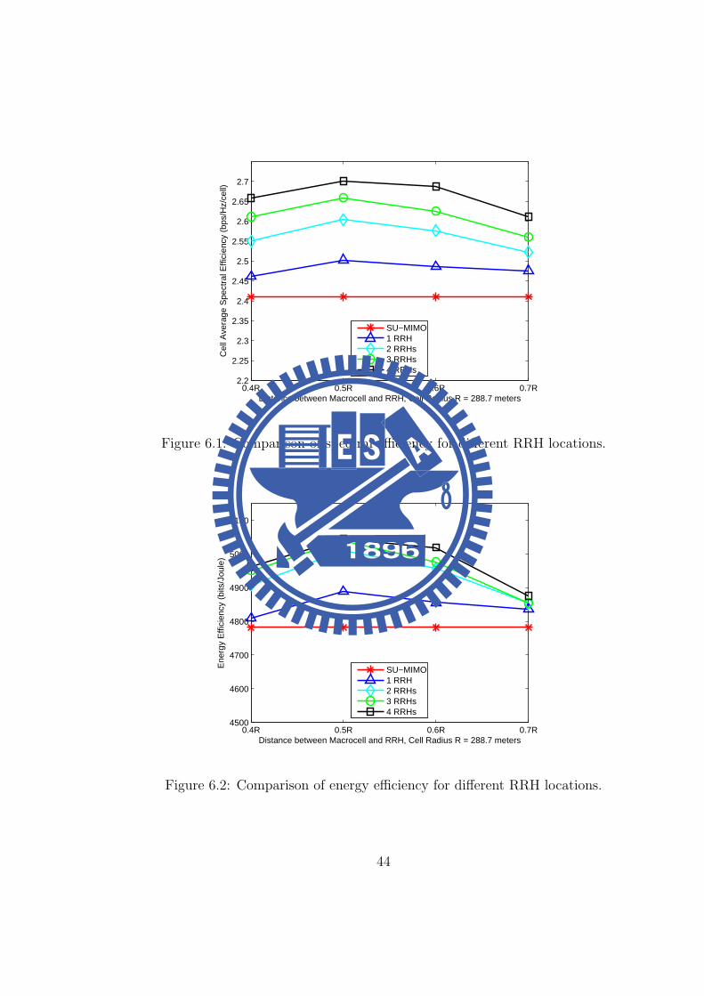
We notice that different RRH positions yield various system performances. In this

section, we adopt the diamond shape antenna architecture first. As we can see from

Fig. 6.1, when RRHs are placed 144.3 meters (0.5R) away from the macro-cell, the

SE is higher than any other positions regardless of the number of RRHs. If RRHs

are too close to the macro-cell, most UEs are out of RRH coverage. In contrast, if

42

RRHs are located near by the cell boarder, it will cause interference to cell-edge UEs

in other cells. Since the power consumption is fixed despite of different distances

between the RRH and macro-cell, EE is also the highest when RRHs are deployed

at 0.5R. The similar trend of SE polygonal line can be seen in EE at Fig. 6.2.

Thus, RRHs are always deployed 144.3 meters (0.5R) away from the macro-cell in

the following simulations so as to achieve better SE and EE. The EE gain of 4 RRHs

over SU-MIMO is 12 %, and the SE gain of 4 RRHs is 5.4 %.

43

0.4R 0.5R 0.6R 0.7R2.2

2.25

2.3

2.35

2.4

2.45

2.5

2.55

2.6

2.65

2.7

Distance between Macrocell and RRH, Cell Radius R = 288.7 meters

Cel

l Ave

rage

Spe

ctra

l Effi

cien

cy (

bps/

Hz/

cell)

SU−MIMO1 RRH2 RRHs3 RRHs4 RRHs

Figure 6.1: Comparison of spectral efficiency for different RRH locations.

0.4R 0.5R 0.6R 0.7R4500

4600

4700

4800

4900

5000

5100

Distance between Macrocell and RRH, Cell Radius R = 288.7 meters

Ene

rgy

Effi

cien

cy (

bits

/Jou

le)

SU−MIMO1 RRH2 RRHs3 RRHs4 RRHs

Figure 6.2: Comparison of energy efficiency for different RRH locations.

44

6.3.2 Effect of Cell Architecture

Different cell structures have various impacts on the system performance. Spectral

and energy efficiency comparison of different system architectures are shown in Figs.

6.4 and 6.3. We find that all the cell architectures have the same trend in both SE and

EE curve. The best location for RRH to achieve the highest SE and EE is at 0.5-0.6R,

where R is the cell radius. Moreover, the performance of narrow beam is the best,

and the diamond shape is the worst. Because three adjacent directional antennas

are facing toward the same point in diamond shape architecture, it will cause larger

interference than the other two kinds of antenna pattern. As for narrow beam, it can

avoid causing interference to other cells effectively, and thus it has the best system

performance. When RRHs are deployed at 0.5R, both SE and EE are maximum. The

spectral efficiency of narrow beam is 2.8660 (bps/Hz/cell), which is the highest. The

second one is pentagon shape, which is 2.8363 (bps/Hz/cell). The diamond shape has

the lowest energy efficiency, 2.7012 (bps/Hz/cell). The SE gain of the narrow beam

over diamond shape is up to 7.9%, and the gain of the pentagon-shape is 5.9%. The

energy efficiency of narrow beam is 5352 (bits/Joule), which is also the highest. The

second one is pentagon shape, which is 5296 (bits/Joule). The diamond shape has

the lowest energy efficiency, 5044 (bits/Joule). The SE gain of narrow beam over the

diamond shape is up to 6.1%, and the gain of pentagon shape is 4.9%.

6.3.3 Tradeoff between Spectral and Energy Efficiency

Based on Fig. 6.5, we observe that the system throughput is growing with the

number of RRHs. However, EE does not necessarily increase with the amount of

RRHs. On the contrary, EE stops increasing when RRHs are up to a certain number.

For instance, the system with 8 RRHs has the highest SE, but the EE is just 5279

(bits/Joule), which is lower than the EE of 4 RRHs, e.g., 5357 (bits/Joule). Ac-

45

0.4R 0.5R 0.6R 0.7R2.3

2.4

2.5

2.6

2.7

2.8

2.9

3

Distance between Macrocell and RRH, Cell Radius R = 288.7 meters

Cel

l Ave

rage

Spe

ctra

l Effi

cien

cy (

bps/

Hz/

cell)

Narrow−beamPentagonalDiamond

Figure 6.3: Comparison of spectral efficiency for different system architectures.

0.4R 0.5R 0.6R 0.7R4400

4600

4800

5000

5200

5400

5600

Distance between Macrocell and RRH, Cell Radius R = 288.7 meters

Ene

rgy

Effi

cien

cy (

bits

/Jou

le)

Narrow−beamPentagonalDiamond

Figure 6.4: Comparison of energy efficiency for different system architectures.

46

cording to (1.5), when the increased margin of numerator is smaller than that of the

denominator, the fraction becomes smaller. That is to say, the gain in throughput

is unable to compensate the additional power dissipation, which causes EE degrada-

tion. As the number of RRHs exceeds 4, the gained margin gets smaller. It’s true

that placing more RRHs improves higher spectral efficiency. However, interferences

from RRHs also increase, thereby degrading system throughput. Therefore, although

the system with 4 RRHs does not have the highest SE, its EE is the best. In fact,

no matter how many RRHs are, heterogeneous CoMP systems always outperform

the conventional SU-MIMO system in terms of SE and EE. Namely, although addi-

tional power is needed for the intra-site CoMP scheme, energy can be utilized more

efficiently by the intra-site CoMP scheme. We list gains in spectral efficiency and

accordingly induced energy efficiency variation at Table 6.3.

2.5 2.6 2.7 2.8 2.9 35050

5100

5150

5200

5250

5300

5350

Spectral Efficiency (bps/Hz/Cell)

Ene

rgy

Eff

icie

ncy (

bit

s/J

oule

)

Figure 6.5: Tradeoff between spectral efficiency and energy efficiency of the intra-site

CoMP scheme.

47

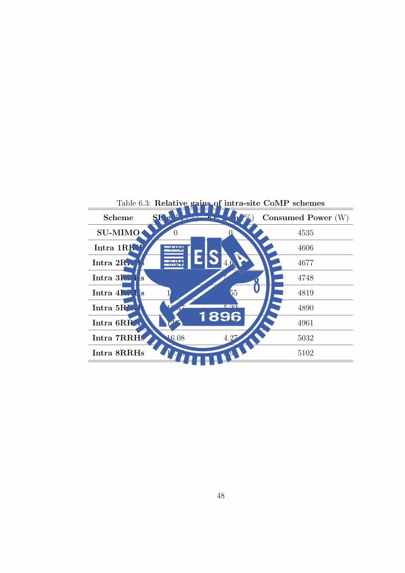
Table 6.3: Relative gains of intra-site CoMP schemes

Scheme SE gain (%) EE gain (%) Consumed Power (W)

SU-MIMO 0 0 4535

Intra 1RRH 3.92 2.17 4606

Intra 2RRHs 8.24 4.69 4677

Intra 3RRHs 10.59 5.34 4748

Intra 4RRHs 12.16 5.55 4819

Intra 5RRHs 13.37 5.22 4890

Intra 6RRHs 14.51 4.65 4961

Intra 7RRHs 16.08 4.27 5032

Intra 8RRHs 17.25 3.98 5102

48

6.4 Inter plus Intra-site CoMP

In the previous section, we demonstrate the overall system throughput and energy

efficiency in intra-site CoMP scenario where neighboring cells still cause great inter-

ference. In order to further reduce the interference, we introduce neighboring sectors

to perform joint transmission or coordinated scheduling/beamforming with the orig-

inal base site. The cooperation of intra-site CoMP scheme is limited only in one

sector, while the cooperation of inter-site CoMP scheme can be across sectors. At the

beginning, we evaluate system performances of inter-site CoMP schemes without the

intra-site coordination and compare that with the conventional SU-MIMO system,

as shown in Fig. 6.6. Despite of additional power for cooperation, the large gain in

spectral efficiency can improve energy efficiency enormously. For the inter-site CS/CB

CoMP, the energy efficiency is up to 5759 (bits/Joule), and it achieves 16.3% gain

over the SU-MIMO system. In addition, the inter-site JP CoMP can also achieve

about 13.5% over the conventional system.

0 0.1 0.2 0.3 0.4 0.5 0.6 0.7 0.80

0.1

0.2

0.3

0.4

0.5

0.6

0.7

0.8

0.9

1

Spectral Efficiency (bps/HZ/UE)

F(x

)

SU−MIMOInter JPInter CB

Figure 6.6: Spectral efficiency comparison of different transmission schemes.

49

Next we combine inter and intra-site CoMP techniques to improve signal qual-

ity of cell-edge UEs and further mitigate interferences from adjacent cells. In the

single UE case, the inter plus intra-site CoMP scheme outperforms the SU-MIMO

transmission scheme and the intra-site CoMP scheme in terms of both SE and EE,

as shown in Fig. 6.7 and Fig. 6.8. The SE of SU-MIMO, intra-site JP, inter JP plus

intra-site JP, and inter CS/CB plus intra-site JP are 2.41 (bps/Hz), 2.86 (bps/Hz),

3.12 (bps/Hz), 3.19 (bps/Hz), respectively. The EE of SU-MIMO, intra-site JP, inter

JP plus intra-site JP, and inter CS/CB plus intra-site JP, are 5077 (bits/Joule), 5352

(bits/Joule), 5775 (bits/Joule), 5915 (bits/Joule), respectively. We set the SU-MIMO

system as comparison baseline. The SE gain of intra-site JP, inter JP plus intra-site

JP, and inter CS/CB plus intra-site JP, are 12%, 25.8%, and 28.7%, respectively.

On the other hand, intra-site JP, inter JP plus intra-site JP, and inter CS/CB plus

intra-site JP can achieve 5.4%, 17.4%, 20.1% EE gain, respectively. For the multiple

UE case, we set the MU-MIMO as comparison baseline. Fig. 6.9 shows that SE gain

of intra-site JP, inter JP plus intra-site JP, and inter CS/CB plus intra-site JP, are

29.7%, 39.1%, and 47%, respectively. On the other hand, Fig. 6.10 shows that intra-

site JP, inter JP plus intra-site JP, and inter CS/CB plus intra-site JP can achieve

23.2%, 29.8%, 37.2% EE gain, respectively.

Because the intra-site CoMP can only enhance the signal by deploying cooper-

ative small cells, the inter-cell interference which put great impacts on cell-edge UEs

still exists. Nevertheless, because the inter-site CoMP can reduce interferences from

nearby macro-cells, the signal quality will be improved significantly. In summary, the

inter-site CS/CB plus intra-site JP with 4 RRHs is the most efficient CoMP scheme.

50

SU−MIMO Intra JP Inter JP+Intra Inter CS/CB+Intra0

0.5

1

1.5

2

2.5

3

3.5

Transmission Schemes

Spe

ctra

l Effi

cien

cy (

bps/

Hz/

cell)

Figure 6.7: Comparison of spectral efficiency for different transmission schemes in the

single UE case.

SU−MIMO Intra JP Inter JP+Intra Inter CS/CB+Intra0

1000

2000

3000

4000

5000

6000

Transmission Schemes

Ene

rgy

Effi

cien

cy (

bits

/Jou

le)

Figure 6.8: Comparison of energy efficiency for different transmission schemes in the

single UE case.

51

MU−MIMO Intra JP Inter JP+Intra Inter CS/CB+Intra0

0.5

1

1.5

2

2.5

3

3.5

4

Transmission Schemes

Spe

ctra

l Effi

cien

cy (

bps/

Hz/

cell)

Figure 6.9: Comparison of spectral efficiency for different transmission schemes in the

multiple UE case.

MU−MIMO Intra JP Inter JP+Intra Inter CS/CB+Intra0

1000

2000

3000

4000

5000

6000

7000

8000

Transmission Schemes

Ene

rgy

Effi

cien

cy (

bits

/Jou

le)

Figure 6.10: Comparison of energy efficiency for different transmission schemes in the

multiple UE case.

52

6.5 Reference Signal Received Power-Based RRH

Selection

According to the previous section, 4 cooperative RRHs yield the highest energy effi-

ciency. However, not every RRH can bring obvious merit to the UE. If a RRH is far

away from the served UE, the received signal quality will be very poor. Hence, the

SE improvement offered by RRHs is little. Moreover, increasing the number of RRH

causes more interferences to UEs in other cells. If we select a RRH which transmits

the largest reference signal received power (RSRP) to the UE, and switch off the other

RRHs in the same sector, both SE and EE will be further improved due to less inter-

ferences and operation power consumption for RRHs. Figs. 6.11 and 6.12 compare

various CoMP schemes with different density of RRH for selection. Besides, we only

choose the RRH with the best signal quality to serve UEs jointly with the macro-cell.

We find that both metrics increase with the density of RRH because UEs are more

likely to be served by a better RRH with the increasing RRH density. However, the

margin of performance gain of deploying 4 RRHs is the highest. When the number of

RRH for selection exceeds 4, the margin of performance gain becomes smaller. Take

the EE margin from 3 to 4 RRHs and the EE margin from 6 to 7 RRHs in intra-site

CoMP case as an example. The differences are 176 (bits/Joule) and 11 (bits/Joule),

respectively. The same phenomenon can be also observed in the intra JP plus inter

JP and the intra JP plus inter CS/CB scheme. Therefore, selecting a serving RRH

from 4 RRHs is the best way to make better energy utilization.

53

1RRH 2RRHs 3RRHs 4RRHs 5RRHs 6RRHs 7RRHs 8RRHs2.6

2.7

2.8

2.9

3

3.1

3.2

3.3

3.4

3.5

Number of RRH

Spe

ctra

l Effi

cien

cy (

bps/

Hz)

Intra JPIntra JP + Inter JPIntra JP + Inter CS/CB

Figure 6.11: Comparison of spectral efficiency for different RRH density with selec-

tion.

1RRH 2RRHs 3RRHs 4RRHs 5RRHs 6RRHs 7RRHs 8RRHs5000

5200

5400

5600

5800

6000

6200

6400

6600

Number of RRH

Ene

rgy

Effi

cien

cy (

bits

/Jou

le)

Intra JPIntra JP + Inter JPIntra JP + Inter CS/CB

Figure 6.12: Comparison of energy efficiency for different RRH density with selection.

54

55

CHAPTER 7

Conclusions

7.1 Thesis Summary

In this thesis, we have evaluated the spectral efficiency and energy efficiency of hier-

archical base station cooperation techniques in heterogeneous networks of the 3GPP

LTE-A system. We proposed a joint system design methodology of system architec-

tures and cooperation schemes for energy-efficient transmission. We focused on two

aspects of BSs, including system architectures and CoMP transmission techniques. In

terms of system architectures, we suggested that RRHs should be deployed at the dis-

tance of 0.5-0.6R (R is the macro cell radius) from the macro cell and adopting narrow

beam antenna architecture to achieve both the highest spectral and energy efficiency.

We also discovered that there exists spectral-energy efficiency tradeoff for small cell

density. It is true that increasing cooperative RRHs yields higher capacity. However,

energy efficiency start declining when the number of RRHs is larger than four. The

reason is that the gain in system throughput cannot compensate the additional power

consumption induced by the increased small cells. Moreover, we can exploit energy

more efficiently by applying the reference signal received power-based RRH selection

method. As for CoMP transmission schemes, the cooperation among BSs not only

enhances the overall throughput, but also improves the energy efficiency compared

to conventional SU-MIMO systems. We considered different levels of CoMP schemes

jointly to obtain an optimal combination. In our cases, the best coordination scheme

is the inter CS/CB plus intra-site JP CoMP scheme. The proposed joint design for

HetNet systems has been revealed by combining the best settings of all aspects. In

summary, we offered the knowledge of how to deploy an energy-efficient system.

7.2 Suggestions for Future Research

For the future research of the thesis, we provide the following suggestions to extend

our work. More precise power consumption models should be taken into consideration

to match realistic situations. For instance, we only consider the number of cooperation

BSs in the signal processing power consumption model for inter-site CoMP. However,

inter-site CoMP techniques include JP and CS/CB, and the corresponding feedback

overhead information as well as the computational complexity will not be the same.

Therefore, different schemes may induce various power consumption, and thus it is

worthy of making a further discussion.

56

57

Bibliography

[1] E. Oh, B. Krishnamachari, X. Liu, and Z. Niu, “Toward dynamic energy-efficientoperation of cellular network infrastructure,” IEEE Commun. Magazine, vol. 49,no. 6, pp. 56–61, Jun. 2011.

[2] W. Vereecken, W. Van Heddeghem, M. Deruyck, B. Puype, B. Lannoo, W.Joseph, D. Colle, L. Martens, and P. Demeester, “Power consumption in telecom-munication networks: overview and reduction strategies,” IEEE Commun. Mag-azine, vol. 49, no. 6, pp. 62–69, Jun. 2011.

[3] Z. Hasan, H. Boostanimehr, and V. K. Bhargava, “Green cellular networks: asurvey, some research issues and challenges,” IEEE Communications SurveysTutorials, vol. 13, no. 4, pp. 524–540, 2011.

[4] H. Bogucka and A. Conti, “Degrees of freedom for energy savings in practicaladaptive wireless systems,” IEEE Commun. Magazine, vol. 49, no. 6, pp. 38–45,Jun. 2011.

[5] Q. Wang, D. Jiang, G. Liu, and Z. Yan, “Coordinated multiple points transmis-sion for LTE-Advanced systems,” in Proc. International Conference on WirelessCommunications, Networking and Mobile Computing, pp. 1–4, Sep. 2009.

[6] L. C. Wang and C. J. Yeh, “A three-cell coordinated network MIMO with frac-tional frequency reuse and directional antennas,” in Proc. IEEE InternationalConference on Communications, pp. 1–5, May 2010.

[7] A. Barbieri, P. Gaal, S. Geirhofer, T. Ji, D. Malladi, Y. Wei, and F. Xue, “Coordi-nated downlink multi-point communications in heterogeneous cellular networks,”in Proc. Information Theory and Applications Workshop, pp. 7–16, Feb. 2012.

[8] Y. Chen, S. Zhang, S. Xu, and G. Y. Li, “Fundamental trade-offs on greenwireless networks,” IEEE Commun. Magazine, vol. 49, no. 6, pp. 30–37, Jun.2011.

[9] G. Miao, N. Himayat, Y. Li, and A. Swami, “Cross-layer optimization for energy-efficient wireless communications: a survey,” Wiley Journal Wireless Communi-cations and Mobile Computing, vol. 9, no. 4, pp. 529–542, Apr. 2009.

[10] C. Han, T. Harrold, S. Armour, I. Krikidis, S. Videv, P. M. Grant, H. Haas ,J.S. Thompson, I. Ku, C. Wang, T. A. Le, M. R. Nakhai, J. Zhang, and L. Hanzo,“Green radio: radio techniques to enable energy-efficient wireless networks,”IEEE Commun. Magazine, vol. 49, no. 6, pp. 46–54, Jun. 2011.

[11] 3GPP, “Technical specification group radio access network; coordinated multi-point operation for LTE physical layer aspects,” 3GPP, Tech. Rep. TR 36.819V11.0.0, Dec. 2011.

[12] C. Khirallah, J. S. Thompson, and D. Vukobratovic, “Energy efficiency of hetero-geneous networks in LTE-Advanced,” in Proc. IEEE Wireless Communicationsand Networking Conference Workshops, pp. 53–58, Apr. 2012.

[13] L. Saker, S. E. Elayoubi, L. Rong, and T. Chahed, “Capacity and energy ef-ficiency of picocell deployment in LTE-A networks,” in Proc. IEEE VehicularTechnology Conference, pp. 1–5, May 2011.

[14] T. Q. S. Quek, W. C. Cheung, and M. Kountouris, “Energy efficiency analysisof two-tier heterogeneous networks,” in Proc. European Wireless Conference, pp.1–5, Apr. 2011.

[15] F. Cao and Z. Fan, “The tradeoff between energy efficiency and system perfor-mance of femtocell deployment,” in Proc. International Symposium on WirelessCommunication Systems, pp. 315–319, Sep. 2010.

[16] Y. Liang, A. Goldsmith, G. Foschini, R. Valenzuela, and D. Chizhik, “Evolutionof base stations in cellular networks: denser deployment versus coordination,” inProc. IEEE International Conference on Communications, pp. 4128–4132, May2008.

[17] A. J. Fehske, P. Marsch, and G. P. Fettweis, “Bit per joule efficiency of cooperat-ing base stations in cellular networks,” in Proc. IEEE GLOBECOM Workshops,pp. 1406–1411, Dec. 2010.

[18] C. Khirallah, D. Vukobratovic, and J. Thompson, “On energy efficiency of jointtransmission coordinated multi-point in LTE-Advanced,” in Proc. InternationalITG Workshop on Smart Antennas, pp. 54–61, Mar. 2012.

[19] 3GPP, “Evolved universal terrestrial radio access (E-UTRA); further advance-ments for E-UTRA physical layer aspects,” 3GPP, Tech. Rep. TR 36.814 V9.0.0,Mar. 2010.

[20] F. Khan, LTE for 4G Mobile Broadband: Air Interface Technologies and Perfor-mance. Cambridge University Press, 2009.

[21] Documents provided by Chunghwa telecom laboratories.

58

[22] Q. Wang, D. Jiang, J. Jin, G. Liu, Z. Yan, and D. Yang, “Application ofBBU+RRU based CoMP system to LTE-Advanced,” in Proc. IEEE Interna-tional Conference on Communications Workshops, pp. 1–5, Jun. 2009.

[23] NTT DOCOMO, Alcatel-Lucent, Alcatel-Lucent Shanghai Bell, Ericsson, andTelecom Italia, “Base station power model,” 3GPP, Tech. Rep. R1-113495, Oct.2011.

[24] G. Auer, V. Giannini, C. Desset, I. Godor, P. Skillermark, M. O. M. A. Imran,D. Sabella, M. J. Gonzalez, O. Blume, and A. Fehske, “How much energy isneeded to run a wireless network?” IEEE Wireless Communications Magzine,vol. 18, no. 5, pp. 40–49, Oct. 2011.

[25] 3GPP, “Physical layer aspects for evolved universal terrestrial radio access (E-UTRA),” 3GPP, Tech. Rep. TR 25.814 V7.1.0, Sep. 2006.

[26] 3GPP, “Evolved universal terrestrial radio access (E-UTRA) physical layer pro-cedures,” 3GPP, Tech. Rep. TS 36.213 V9.3.0, Sep. 2010.

[27] J. C. Ikuno, M. Wrulich, and M. Rupp, “System level simulation of LTE net-works,” in Proc. IEEE Vehicular Technology Conference, pp. 1–5, May 2010.

[28] Y. J. Liu, T. T. Chiang, and L. C. Wang, “Physical layer performance calibrationfor 3GPP LTE-A systems,” in Proc. IEEE Asia Pacific Wireless CommunicationSymposium, Aug. 2011.

[29] L. C. Wang, “A new cellular architecture based on an interleaved cluster con-cept,” IEEE Transactions on Vehicular Technology, vol. 48, no. 6, pp. 1809–1818,Nov. 1999.

[30] NTT DOCOMO, “Summary of evaluation results for 3GPP requirements,”3GPP, Tech. Rep. R1-100823, Jan. 2010.

59

Vita

Tsung-Chan Hsieh received his B.S. degree from the Department of Com-munication Engineering, National Chiao-Tung University, Taiwan, R.O.C., in 2010.From July 2010 to August 2012, he worked his Master degree in the Mobile Commu-nications and Cloud Computing Lab at the Institute of Communications Engineeringat National Chiao-Tung University. His research interests are in the field of wirelesscommunications.

60