Embed Size (px)
Citation preview

ÉCOLE DE TECHNOLOGIE SUPÉRIEURE UNIVERSITÉ DU QUÉBEC
THESIS PRESENTED TO ÉCOLE DE TECHNOLOGIE SUPÉRIEURE
IN PARTIAL FULFILLMENT OF THE REQUIREMENTS FOR THE DEGREE OF DOCTOR OF PHILOSOPHY
Ph.D.
BY Ahmad ABO EL EZZ
PROBABILISTIC SEISMIC VULNERABILITY AND RISK ASSESSMENT OF STONE MASONRY STRUCTURES
MONTREAL, 24 APRIL 2013
© Copyright 2013 reserved by Ahmad Abo El Ezz
Ahmad Abo El Ezz, 2013

This Creative Commons licence allows readers to download this work and share it with others as long as the author is credited. The content of this work can’t be modified in any way or used commercially.

BOARD OF EXAMINERS (THESIS PH.D.)
THIS THESIS HAS BEEN EVALUATED
BY THE FOLLOWING BOARD OF EXAMINERS Prof. Marie-José Nollet, Thesis Supervisor Département de génie de la construction à l’École de technologie supérieure Dr. Miroslav Nastev, Thesis Co-supervisor Geological Survey of Canada, Natural Resources Canada Prof. Éric David, President of the Board of Examiners Département de génie mécanique à l’École de technologie supérieure Prof. Omar Chaallal, Member of the Board of Examiners Département de génie de la construction à l’École de technologie supérieure Prof. Pierino Lestuzzi , External Member of the Board of Examiners École Polytechnique Fédérale de Lausanne, Switzerland
THIS THESIS WAS PRENSENTED AND DEFENDED
IN THE PRESENCE OF A BOARD OF EXAMINERS AND PUBLIC
16 APRIL 2013
AT ÉCOLE DE TECHNOLOGIE SUPÉRIEURE


ACKNOWLEDGMENT
I would like to express my sincere gratitude and appreciation to my PhD supervisor Professor
Marie-José Nollet and co-supervisor Dr. Miroslav Nastev for their continuous guidance,
support and encouragement throughout the course of my studies. I am very grateful to them
for the education and direction they have provided.
This PhD study was supported by Natural Resources Canada, Geological Survey of Canada
through the Public Safety Geoscience Program, and the Chemical, Biological, Radiological,
Nuclear and Explosives Research and Technology Initiative, administered by the Defence
R&D Canada, Centre for Security Science. This financial support is gratefully
acknowledged.
I would like to thank my colleagues at the Construction Engineering Department at the ETS
Montreal especially Suze Youance and Bertrand Galy for their help and friendship.
I would like to thank my wife Shimaa for her help, support and encouragement and my son
Yossef for being a source of motivation.


ÉVALUATION PROBABILISTE DE LA VULNÉRABILITÉ ET DES RISQUES SISMIQUES DES BÂTIMENTS EN MAÇONNERIE DE PIERRE
Ahmad ABO EL EZZ
RÉSUMÉ
Parmi les risques naturels, les tremblements de terre ont une incidence significative sur l'environnement bâti et engendrent des pertes économiques et sociales. Les pertes élevées causées par les derniers tremblements de terre destructeurs mettent en évidence la nécessité d'une évaluation de la vulnérabilité sismique des bâtiments existants. Parmi les bâtiments les plus vulnérables, les bâtiments anciens en maçonnerie de pierre sont nombreux dans les centres historiques urbains de l'Est du Canada, comme le Vieux-Québec, et représentent un patrimoine architectural et culturel dont la valeur est difficilement mesurable. Ces bâtiments ont été construits pour résister aux charges de gravité et offrent généralement une faible résistance aux charges sismiques. L’évaluation de leur vulnérabilité sismique est donc la première étape nécessaire au développement d’un programme de mitigation du risque et de mise à niveau sismique. L'objectif de cette étude est de développer un ensemble d’outils analytiques probabilistes pour l'évaluation de la vulnérabilité sismique des bâtiments en maçonnerie de pierre et l’analyse efficace des incertitudes inhérentes au processus d’évaluation. En premier lieu, une approche méthodologique simplifiée est proposée pour la modélisation de la vulnérabilité des bâtiments et le traitement systématique des incertitudes. Les courbes de capacité sont développées à l’aide d’un modèle mécanique équivalent à un degré de liberté. Les courbes de fragilité, donnant le degré de dommages en fonction du déplacement spectral, sont développées sur la base de déplacements critiques des murs de maçonnerie de pierre. Une analyse probabiliste simplifiée de la demande sismique est proposée pour déterminer l’influence de l'incertitude combinée de la capacité et de la demande sur les courbes de fragilité. En deuxième lieu, une procédure pour le développement de fonctions de fragilité et de vulnérabilité sismique en termes d’une mesure d’intensité indépendante de la structure (l'accélération spectrale) est proposée. La procédure est efficace pour réaliser rapidement l’évaluation de la vulnérabilité des bâtiments en maçonnerie de pierre et peut facilement être adaptée et appliquée à une autre classe de bâtiment. En troisième lieu, une analyse de sensibilité est réalisée pour quantifier l’influence des incertitudes associées aux paramètres utilisées dans la procédure de modélisation de la vulnérabilité sismique. Finalement, la méthodologie proposée est appliquée à l’estimation des dommages pour 1220 bâtiments existants du Vieux-Québec selon un scénario sismique de magnitude 6,2 à une distancé épicentrale de 15km pour une probabilité de dépassement de 2% en 50 ans. Les courbes de fragilité des autres types de bâtiments ont été développées avec la procédure proposée à partir des courbes de capacité proposées dans Hazus. Ce scénario montre que la plupart des dommages prévus sont concentrés aux vieux bâtiments de maçonnerie de brique non-armée et aux bâtiments en maçonnerie de pierre. Mots clés: vulnérabilité sismique, maçonnerie de pierre, analyse de l'incertitude.


PROBABILISTIC SEISMIC VULNERABILITY AND RISK ASSESSMENT OF
STONE MASONRY STRUCTURES
Ahmad ABO EL EZZ
ABSTRACT
Earthquakes represent major natural hazards that regularly impact the built environment in seismic prone areas worldwide and cause considerable social and economic losses. The high losses incurred following the past destructive earthquakes promoted the need for assessment of the seismic vulnerability and risk of the existing buildings. Many historic buildings in the old urban centers in Eastern Canada such as Old Quebec City are built of stone masonry and represent un-measurable architectural and cultural heritage. These buildings were built to resist gravity loads only and generally offer poor resistance to lateral seismic loads. Seismic vulnerability assessment of stone masonry buildings is therefore the first necessary step in developing seismic retrofitting and pre-disaster mitigation plans. The objective of this study is to develop a set of probability-based analytical tools for efficient seismic vulnerability and uncertainty analysis of stone masonry buildings. A simplified probabilistic analytical methodology for vulnerability modelling of stone masonry building with systematic treatment of uncertainties throughout the modelling process is developed in the first part of this study. Building capacity curves are developed using a simplified mechanical model. A displacement based procedure is used to develop damage state fragility functions in terms of spectral displacement response based on drift thresholds of stone masonry walls. A simplified probabilistic seismic demand analysis is proposed to capture the combined uncertainty in capacity and demand on fragility functions. In the second part, a robust analytical procedure for the development of seismic hazard compatible fragility and vulnerability functions is proposed. The results are given by sets of seismic hazard compatible vulnerability functions in terms of structure-independent intensity measure (e.g. spectral acceleration) that can be used for seismic risk analysis. The procedure is very efficient for conducting rapid vulnerability assessment of stone masonry buildings. With modification of input structural parameters, it can be adapted and applied to any other building class. A sensitivity analysis of the seismic vulnerability modelling is conducted to quantify the uncertainties associated with each of the input parameters. The proposed methodology was validated for a scenario-based seismic risk assessment of existing buildings in Old Quebec City. The procedure for hazard compatible vulnerability modelling was used to develop seismic fragility functions in terms of spectral acceleration representative of the inventoried buildings. A total of 1220 buildings were considered. The assessment was performed for a scenario event of magnitude 6.2 at distance 15km with a probability of exceedance of 2% in 50 years. The study showed that most of the expected damage is concentrated in the old brick and stone masonry buildings. Keywords: Seismic vulnerability, fragility functions, stone masonry, uncertainty analysis.


TABLE OF CONTENTS
Page
INTRODUCTION .....................................................................................................................1�
CHAPTER 1 LITERATURE REVIEW ............................................................................9�1.1� Introduction ....................................................................................................................9�1.2� Fragility and vulnerability functions ............................................................................11�1.3� Analytical vulnerability modelling and uncertainty quantification .............................12�1.4� Structural analysis ........................................................................................................16�1.5� Structural modelling of seismic capacity for masonry buildings.................................19�
1.5.1� Seismic response mechanisms of masonry buildings ............................... 19�1.5.2� Capacity modelling methods..................................................................... 23�
1.6� Damage analysis ..........................................................................................................27�1.7� Loss analysis ................................................................................................................30�1.8� Review of existing vulnerability models for stone masonry buildings........................31�1.9� Summary ......................................................................................................................34�
CHAPTER 2 DISPLACEMENT BASED FRAGILITY ANALYSIS ............................37�2.1� Introduction ..................................................................................................................37�2.2� Analytical displacement fragility functions .................................................................37�2.3� Inventory ......................................................................................................................38�2.4� Displacement based damage model .............................................................................41�2.5� Capacity model ............................................................................................................47�2.6� Seismic demand model ................................................................................................54�2.7� Fragility based damage assessment .............................................................................62�2.8� Summary and conclusions ...........................................................................................64�
CHAPTER 3 HAZARD COMPATIBLE VULNERABILITY MODELLING ..............67�3.1� Introduction ..................................................................................................................67�3.2� Vulnerability modelling procedure ..............................................................................67�3.3� Scenario based vulnerability assessment .....................................................................74�3.4� Summary and conclusions ...........................................................................................80�
CHAPTER 4 SENSITIVITY ANALYSIS ON VULNERABILITY MODELLING......81�4.1� Introduction ..................................................................................................................81�4.2� Variation in structural parameters ................................................................................82�4.3� Variation in damage parameters ..................................................................................83�4.4� Variation in loss parameters.........................................................................................84�4.5� Sensitivity analysis results ...........................................................................................85�4.6� Discussion of the sensitivity analysis results ...............................................................88�
4.6.1� Structural parameters ................................................................................ 88�4.6.2� Damage parameters ................................................................................... 89�4.6.3� Loss parameters ........................................................................................ 90�
XII
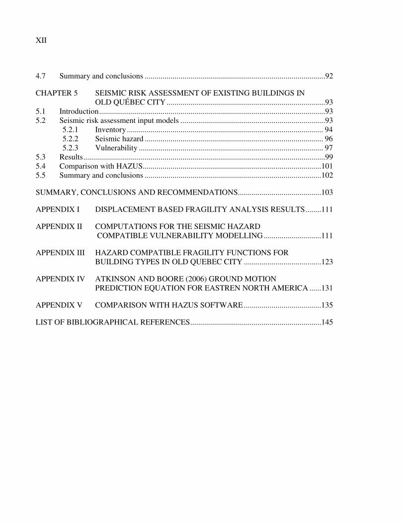
4.7� Summary and conclusions ...........................................................................................92�
CHAPTER 5 SEISMIC RISK ASSESSMENT OF EXISTING BUILDINGS IN OLD QUÉBEC CITY ................................................................................93�
5.1� Introduction ..................................................................................................................93�5.2� Seismic risk assessment input models .........................................................................93�
5.2.1� Inventory ................................................................................................... 94�5.2.2� Seismic hazard .......................................................................................... 96�5.2.3� Vulnerability ............................................................................................. 97�
5.3� Results ..........................................................................................................................99�5.4� Comparison with HAZUS..........................................................................................101�5.5� Summary and conclusions .........................................................................................102�
SUMMARY, CONCLUSIONS AND RECOMMENDATIONS..........................................103�
APPENDIX I DISPLACEMENT BASED FRAGILITY ANALYSIS RESULTS ........111�
APPENDIX II COMPUTATIONS FOR THE SEISMIC HAZARD COMPATIBLE VULNERABILITY MODELLING .............................111�
APPENDIX III HAZARD COMPATIBLE FRAGILITY FUNCTIONS FOR BUILDING TYPES IN OLD QUEBEC CITY .......................................123�
APPENDIX IV ATKINSON AND BOORE (2006) GROUND MOTION PREDICTION EQUATION FOR EASTREN NORTH AMERICA ......131�
APPENDIX V COMPARISON WITH HAZUS SOFTWARE .......................................135�
LIST OF BIBLIOGRAPHICAL REFERENCES ..................................................................145�
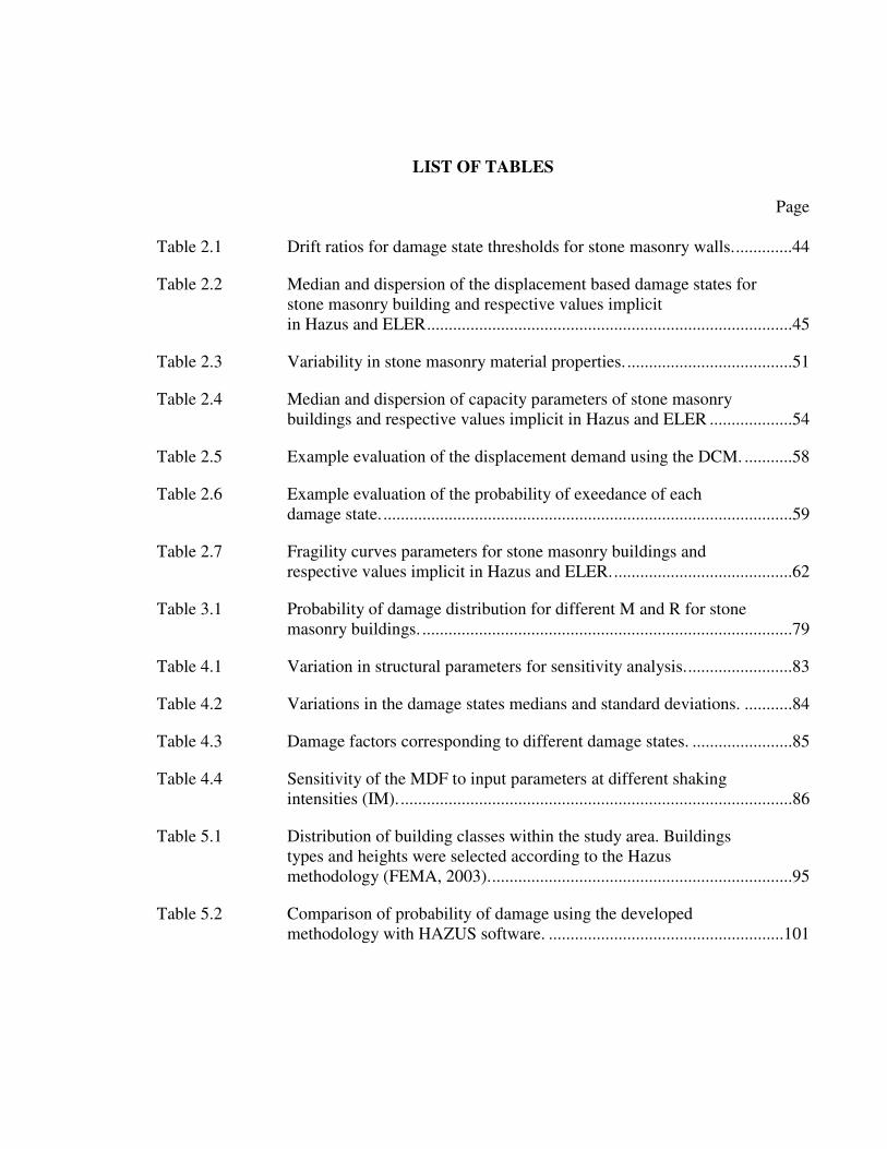
LIST OF TABLES
Page Table 2.1 Drift ratios for damage state thresholds for stone masonry walls. .............44�
Table 2.2 Median and dispersion of the displacement based damage states for stone masonry building and respective values implicit in Hazus and ELER ....................................................................................45�
Table 2.3 Variability in stone masonry material properties. ......................................51�
Table 2.4 Median and dispersion of capacity parameters of stone masonry buildings and respective values implicit in Hazus and ELER ...................54�
Table 2.5 Example evaluation of the displacement demand using the DCM. ...........58�
Table 2.6 Example evaluation of the probability of exeedance of each damage state. ..............................................................................................59�
Table 2.7 Fragility curves parameters for stone masonry buildings and respective values implicit in Hazus and ELER. .........................................62�
Table 3.1 Probability of damage distribution for different M and R for stone masonry buildings. .....................................................................................79�
Table 4.1 Variation in structural parameters for sensitivity analysis. ........................83�
Table 4.2 Variations in the damage states medians and standard deviations. ...........84�
Table 4.3 Damage factors corresponding to different damage states. .......................85�
Table 4.4 Sensitivity of the MDF to input parameters at different shaking intensities (IM). ..........................................................................................86�
Table 5.1 Distribution of building classes within the study area. Buildings types and heights were selected according to the Hazus methodology (FEMA, 2003). .....................................................................95�
Table 5.2 Comparison of probability of damage using the developed methodology with HAZUS software. ......................................................101�


LIST OF FIGURES
Page
Figure 1.1 Framework for seismic risk assessment. ....................................................10�
Figure 1.2 Damageability functions: (a) sample fragility functions and (b) vulnerability function. ................................................................................11�
Figure 1.3 Framework for analytical vulnerability modelling. ..................................13�
Figure 1.4 Illustration of the required input parameters for nonlinear static structural analysis method. .........................................................................15�
Figure 1.5 Illustration of required input parameters for nonlinear dynamic structural analysis method. .........................................................................15�
Figure 1.6 Illustration of the capacity spectrum method. ............................................18�
Figure 1.7 Illustration of the displacement coefficient method. .................................18�
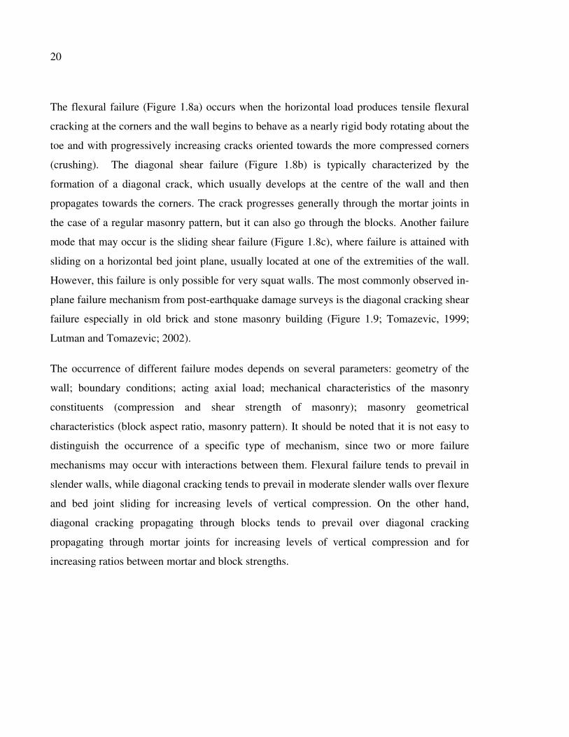
Figure 1.8 In-plane failure mechanisms of masonry walls: (a) flexural failure, (b) diagonal shear failure and (c) sliding shear failure ..............................21�
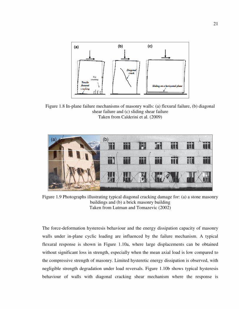
Figure 1.9 Photographs illustrating typical diagonal cracking damage for: (a) a stone masonry buildings and (b) a brick masonry building ...............21�
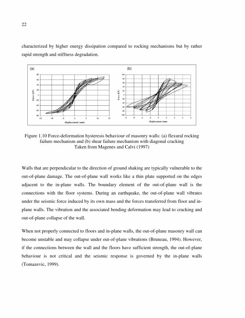
Figure 1.10 Force-deformation hysteresis behaviour of masonry walls: (a) flexural rocking failure mechanism and (b) shear failure mechanism with diagonal cracking. ...........................................................22�
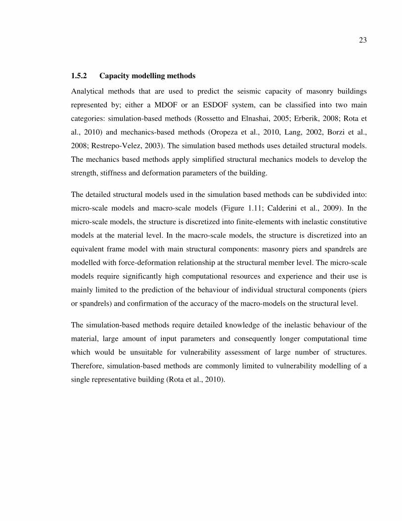
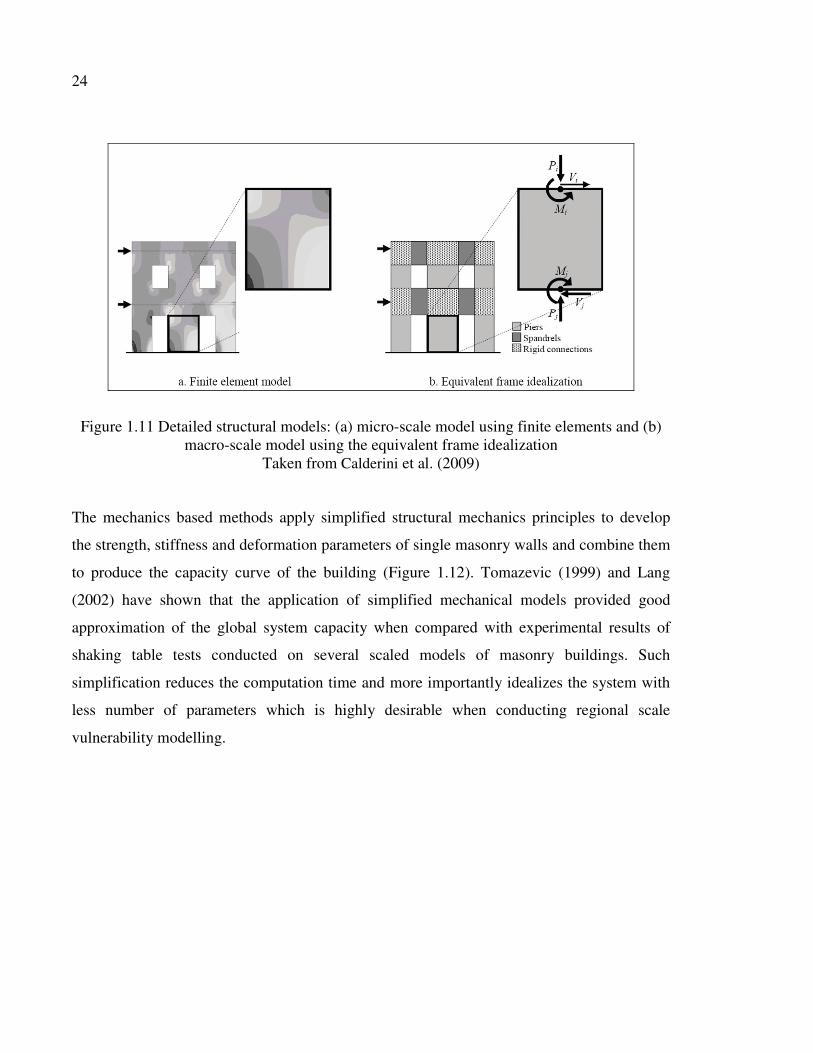
Figure 1.11 Detailed structural models: (a) micro-scale model using finite elements and (b) macro-scale model using the equivalent frame idealization .................................................................................................24�
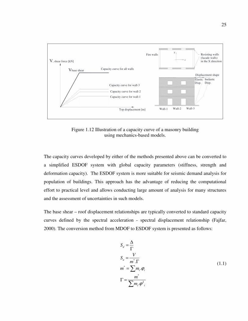
Figure 1.12 Illustration of a capacity curve of a masonry building using mechanics-based models. ...........................................................................25�
Figure 1.13 Illustration of the conversion of the MDOF system to an ESDOF: (a) the mode shape and mass distribution and (b) the conversion of the capacity curve to the spectral acceleration-displacement domain. ......26�
Figure 1.14 Identification of the drift thresholds that corresponds to reaching a specific damage state. ..............................................................................28�
XVI
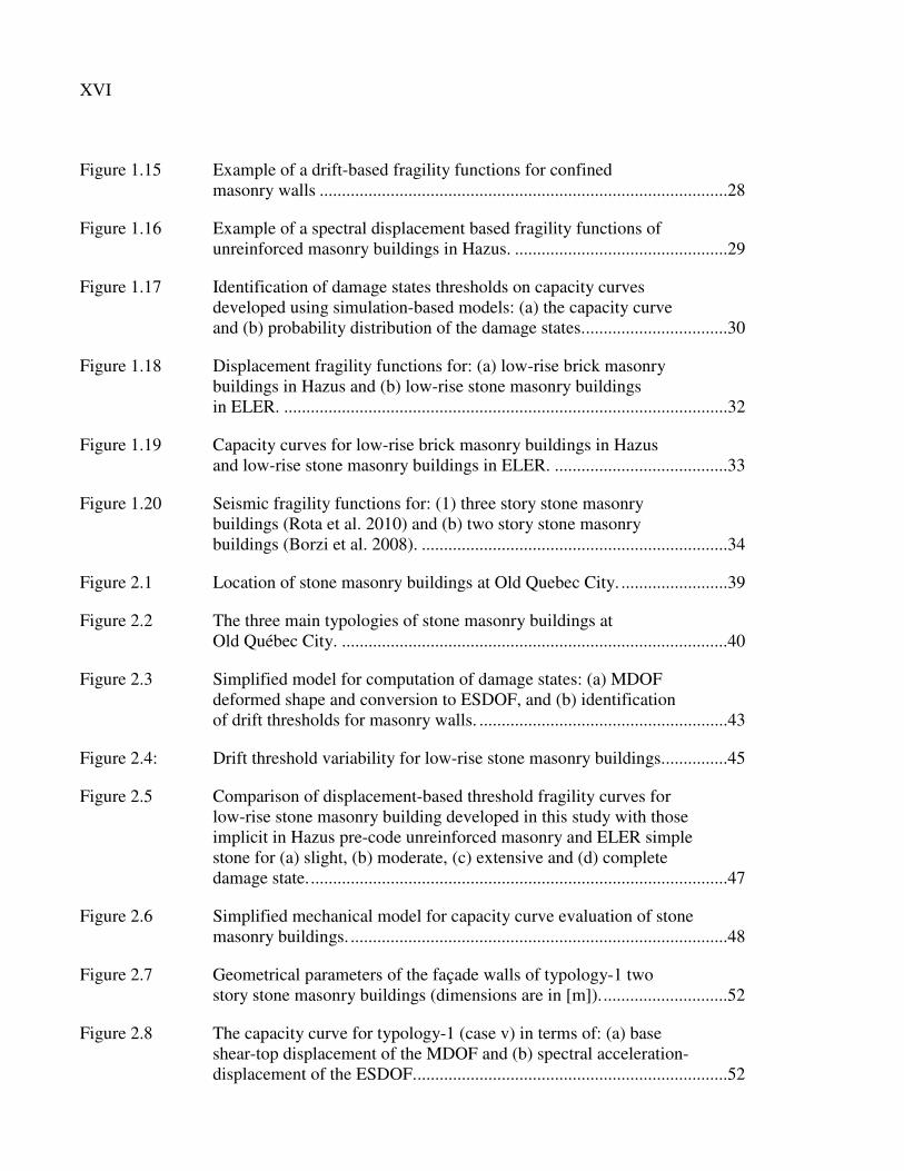
Figure 1.15 Example of a drift-based fragility functions for confined masonry walls ............................................................................................28�
Figure 1.16 Example of a spectral displacement based fragility functions of unreinforced masonry buildings in Hazus. ................................................29�
Figure 1.17 Identification of damage states thresholds on capacity curves developed using simulation-based models: (a) the capacity curve and (b) probability distribution of the damage states. ................................30�
Figure 1.18 Displacement fragility functions for: (a) low-rise brick masonry buildings in Hazus and (b) low-rise stone masonry buildings in ELER. ....................................................................................................32�
Figure 1.19 Capacity curves for low-rise brick masonry buildings in Hazus and low-rise stone masonry buildings in ELER. .......................................33�
Figure 1.20 Seismic fragility functions for: (1) three story stone masonry buildings (Rota et al. 2010) and (b) two story stone masonry buildings (Borzi et al. 2008). .....................................................................34�
Figure 2.1 Location of stone masonry buildings at Old Quebec City. ........................39�
Figure 2.2 The three main typologies of stone masonry buildings at Old Québec City. .......................................................................................40�
Figure 2.3 Simplified model for computation of damage states: (a) MDOF deformed shape and conversion to ESDOF, and (b) identification of drift thresholds for masonry walls. ........................................................43�
Figure 2.4: Drift threshold variability for low-rise stone masonry buildings...............45�
Figure 2.5 Comparison of displacement-based threshold fragility curves for low-rise stone masonry building developed in this study with those implicit in Hazus pre-code unreinforced masonry and ELER simple stone for (a) slight, (b) moderate, (c) extensive and (d) complete damage state. ..............................................................................................47�
Figure 2.6 Simplified mechanical model for capacity curve evaluation of stone masonry buildings. .....................................................................................48�
Figure 2.7 Geometrical parameters of the façade walls of typology-1 two story stone masonry buildings (dimensions are in [m]). ............................52�
Figure 2.8 The capacity curve for typology-1 (case v) in terms of: (a) base shear-top displacement of the MDOF and (b) spectral acceleration-displacement of the ESDOF. ......................................................................52�

XVII
Figure 2.9 Capacity curves for stone masonry typology with varying material properties and comparison with respective median capacity curves implicit in Hazus and ELER. .....................................................................53�
Figure 2.10 Illustration of the procedure to calculate the inelastic spectral displacement demand using the DCM. ......................................................56�
Figure 2.11 Illustration of the variability in displacement demand at a given level of PGA. .............................................................................................57�
Figure 2.12 Seismic demand model: (a) lognormal distribution of the inelastic displacement demand for various levels of PGA (black arrow indicates PGA with 2%/50 years for Quebec city for soil-class B), and (b) evaluation of the probability of exceedance a specific damage state. ..............................................................................................59�
Figure 2.13 Mapping between the probabilities points in terms of PGA to spectral displacement. .............................................................................................60�
Figure 2.14 Fitting of the probability distribution of combined uncertainty of capacity and demand parameters for different damage state (a) the standard normal variable domain and (b) the cumulative lognormal functions. ..................................................................................61�
Figure 2.15 Fragility based damage assessment for a spectral displacement corresponding to uniform hazard spectrum with probability of 2%/50 years: (a) fragility curves for low-rise two-story stone masonry buildings in Old Québec City and (b) respective damage state probabilities compared with those obtained with fragility curves implicit in Hazus and ELER. ..........................................................63�
Figure 3.1 Vulnerability modelling procedure. ...........................................................68�
Figure 3.2 Illustration of the evaluation of the performance point in the CSM. .........70�
Figure 3.3 Illustration of the mapping of damage state probabilities from: (a) the spectral displacement response, to (b) to the structure- independent IM fragility function. .............................................................72�
Figure 3.4 Illustration of the mapping from the seismic fragility function (a) to the vulnerability function (b). ...........................................................73�
Figure 3.5 Idealized response spectra for scenario earthquakes using Sa0.3 sec and Sa1.0 sec values from AB06 GMPE. M is moment magnitude and R is hypocentral distance in km. .......................................74�
XVIII
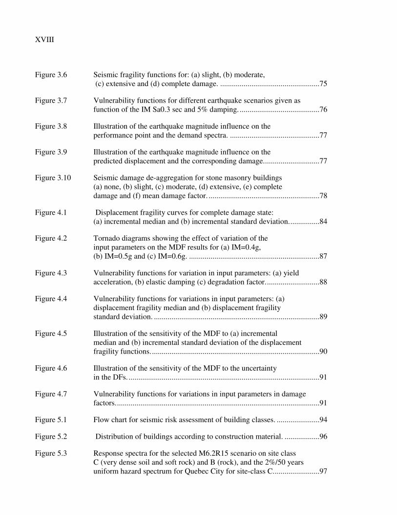
Figure 3.6 Seismic fragility functions for: (a) slight, (b) moderate, (c) extensive and (d) complete damage. ...................................................75�
Figure 3.7 Vulnerability functions for different earthquake scenarios given as function of the IM Sa0.3 sec and 5% damping. .........................................76�
Figure 3.8 Illustration of the earthquake magnitude influence on the performance point and the demand spectra. ..............................................77�
Figure 3.9 Illustration of the earthquake magnitude influence on the predicted displacement and the corresponding damage. ............................77�
Figure 3.10 Seismic damage de-aggregation for stone masonry buildings (a) none, (b) slight, (c) moderate, (d) extensive, (e) complete damage and (f) mean damage factor. .........................................................78�
Figure 4.1 Displacement fragility curves for complete damage state: (a) incremental median and (b) incremental standard deviation. ...............84�
Figure 4.2 Tornado diagrams showing the effect of variation of the input parameters on the MDF results for (a) IM=0.4g, (b) IM=0.5g and (c) IM=0.6g. ...................................................................87�
Figure 4.3 Vulnerability functions for variation in input parameters: (a) yield acceleration, (b) elastic damping (c) degradation factor. ...........................88�
Figure 4.4 Vulnerability functions for variations in input parameters: (a) displacement fragility median and (b) displacement fragility standard deviation. .....................................................................................89�
Figure 4.5 Illustration of the sensitivity of the MDF to (a) incremental median and (b) incremental standard deviation of the displacement fragility functions. ......................................................................................90�
Figure 4.6 Illustration of the sensitivity of the MDF to the uncertainty in the DFs. ..................................................................................................91�
Figure 4.7 Vulnerability functions for variations in input parameters in damage factors. ........................................................................................................91�
Figure 5.1 Flow chart for seismic risk assessment of building classes. ......................94�
Figure 5.2 Distribution of buildings according to construction material. ..................96�
Figure 5.3 Response spectra for the selected M6.2R15 scenario on site class C (very dense soil and soft rock) and B (rock), and the 2%/50 years uniform hazard spectrum for Quebec City for site-class C. .......................97�
XIX
Figure 5.4 Fragility functions for (a) low-rise stone masonry buildings, and (b) low-rise brick masonry buildings. ........................................................98�
Figure 5.5 Total number of buildings in each damage state for a scenario event M6.2R15. ...................................................................................................99�
Figure 5.6 Proportion of buildings by construction material type in each damage state for a scenario event M6.2R15. ...........................................100�

LIST OF ABREVIATIONS
ATC Applied technology council
C1L Concrete moment frame low rise
CSM Capacity spectrum method
DCM Displacement coefficient method
DF Damage factor
DS Damage state
ELER Earthquake loss estimation routine
ESDOF Equivalent single degree of freedom
GMPE Ground motion prediction equation
HAZUS Hazards United States loss estimation method
IM Intensity measure
MDF Mean damage factor
MDOF Multi-degree of freedom
NLSA Nonlinear static analysis
NLTHA Nonlinear time history analysis
PGA Peak ground acceleration
S1L Steel moment frame low rise
S2L Steel braced frames low rise
S5L Steel frames with URM infill low rise
URM Unreinforced masonry
URMB Unreinforced brick masonry
URMS Unreinforced stone masonry
W1L Wood light frame low rise
UHS Uniform hazard spectrum
NBCC National building code of Canada


LIST OF SYMBOLS Sd Spectral displacement
Sa Spectral acceleration
Say Spectral acceleration at the yield point of a capacity curve
k Degradation factor
� Median value
� Log-Standard deviation
�ds Median value for a specific damage state
�ds Logarithmic standard deviation of a specific damage state
� Cumulative standard normal distribution function
�e Elastic damping ratio
�eff Effective damping ratio
H Total height of the building
hs Height of the first story
Vr Shear strength corresponding to the flexural rocking failure
Vdt Shear strength corresponding to diagonal cracking failure
L Masonry wall length
t Masonry wall thickness
T Period of vibration
Ty Yield period of vibration
� Inter-story drift
�DS Inter-story drift at the threshold of a specific damage state
� Displacement at the top of a wall
EIeff Effective flexural stiffness
GAeff Effective shear stiffness
fm Masonry compression strength
fdt Masonry shear strength corresponding to diagonal cracking
Em Masonry elastic modulus
Gm Masonry shear modulus
� Modal participation factor
XXIV
M Earthquake scenario magnitude
R Earthquake scenario epicentral distance
Fa Soil-site amplification factor for the constant-acceleration portion
Fv Soil-site amplification factor for the constant-velocity portion
RA Damping reduction factor for damping ratios more than 5% for constant-
acceleration portion
RV Damping reduction factor for damping ratios more than 5% for constant-
velocity portion
TAVD The period at the intersection of the constant-acceleration and constant-
velocity portions of the demand spectrum
g Gravitational acceleration

INTRODUCTION
Context
Earthquakes represent a major natural hazard that regularly impact the built environment in
seismic prone areas worldwide and cause social and economic losses. Recent earthquakes,
e.g., 2009 L’Aquila earthquake in Italy and 2010 Christchurch earthquake in New Zealand,
showed that most of the damage and economic losses are related to old vulnerable masonry
buildings (Ingham and Griffith, 2011). The high losses incurred due to destructive
earthquakes promoted the need for assessment of the performance of existing buildings under
potential future earthquake events. This requires improved seismic vulnerability and risk
assessment tools to assist informed decision making with the objective to minimize potential
risks and to develop emergency response and recovery strategies.
In Eastern Canada, most of the existing buildings were constructed before the introduction of
the seismic provisions in building codes. In particular, pre-code masonry buildings types are
predominant in dense urban centers such as Quebec City and Montreal in the Province of
Quebec. The potential economic and social losses due to strong earthquake events can thus
be extensive. On the other hand, although masonry buildings represent major and most
vulnerable part of the existing building stock, less research was devoted to study the seismic
vulnerability of this type of buildings compared to other structural types, e.g. reinforced
concrete and steel buildings.
Typical regional seismic risk assessment studies consist of three major components: hazard,
exposure, and vulnerability of the exposure with respect to the seismic hazard (Coburn and
Spence, 2002). Seismic hazard defines the intensity of the expected earthquake motion at a
particular location over a given time period; exposure identifies the built environment
(buildings and infrastructures) in the area affected by the earthquake; and vulnerability refers
to the exposure susceptibility to earthquake impacts defined by the expected degree of
damage and loss that would result under different levels of seismic loading. The key among
2
these components is the vulnerability modelling. The vulnerability is typically presented with
sets of fragility functions describing the expected physical damage whereas economic losses
are given by vulnerability functions (Porter, 2002). The typical results of risk assessment
comprise estimates of the potential physical damage and direct economic losses.
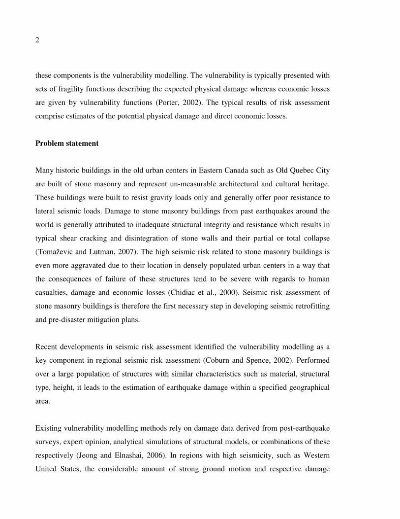
Problem statement
Many historic buildings in the old urban centers in Eastern Canada such as Old Quebec City
are built of stone masonry and represent un-measurable architectural and cultural heritage.
These buildings were built to resist gravity loads only and generally offer poor resistance to
lateral seismic loads. Damage to stone masonry buildings from past earthquakes around the
world is generally attributed to inadequate structural integrity and resistance which results in
typical shear cracking and disintegration of stone walls and their partial or total collapse
(Tomaževic and Lutman, 2007). The high seismic risk related to stone masonry buildings is
even more aggravated due to their location in densely populated urban centers in a way that
the consequences of failure of these structures tend to be severe with regards to human
casualties, damage and economic losses (Chidiac et al., 2000). Seismic risk assessment of
stone masonry buildings is therefore the first necessary step in developing seismic retrofitting
and pre-disaster mitigation plans.
Recent developments in seismic risk assessment identified the vulnerability modelling as a
key component in regional seismic risk assessment (Coburn and Spence, 2002). Performed
over a large population of structures with similar characteristics such as material, structural
type, height, it leads to the estimation of earthquake damage within a specified geographical
area.
Existing vulnerability modelling methods rely on damage data derived from post-earthquake
surveys, expert opinion, analytical simulations of structural models, or combinations of these
respectively (Jeong and Elnashai, 2006). In regions with high seismicity, such as Western
United States, the considerable amount of strong ground motion and respective damage

3
records have been used to build observational and expert opinion based vulnerability
modelling tools. In regions with scarcity of recorded damage data, such as Eastern Canada,
risk assessment relies mainly on analytical vulnerability modelling. The analytical methods
consist of structural modeling and evaluation of the likelihood for a given building to
experience damage from earthquake of a given intensity.
Existing analytical vulnerability models for unreinforced masonry structures were focused on
brick masonry buildings due to availability of experimental data and mechanical models.
Currently, the most widely used North American regional seismic risk assessment tool,
Hazus (FEMA, 2003), reflects the vulnerability information of the construction types present
in the United States. It considers only one structural class for unreinforced masonry buildings
(URM), brick masonry structures with vulnerability information based mainly on expert
judgment and observational data (Kircher et al., 1997a). It has been shown, however, that
Hazus vulnerability model for URM do not adequately represent the response of stone
masonry structures to earthquake loading (Lefebvre, 2004; Abo-El-Ezz et al., 2011b). On the
other hand, only few analytical vulnerability studies of stone masonry buildings are available
in the literature and mainly focused on European building types (Rota et al. 2010; Borzi et
al., 2008). The earthquake loss estimation routine ELER (Erdik et al., 2010), which is mainly
used in Europe, considers stone masonry buildings with vulnerability information mainly
derived based on observed damage data collected from Italian earthquakes and expert
judgment (Giovinazzi, 2005).
Another important issue which merits particular attention are the uncertainties related to the
various parameters used in the in the vulnerability modelling that may have considerable
impact on the risk assessment results. These include: uncertainties due to variability of the
ground motions, uncertainties in seismic demand and capacity of structures due to variations
of their geometry and material properties, and uncertainties in the definition of the damage
states (Choun and Elnashai, 2010). All these uncertainties should be systematically
quantified in the vulnerability modelling in order to provide confidence in the estimated risk
and identify the model sensitivity to input parameters.
4
Objectives and methodology
The main objective of this study is to develop a set of probability-based analytical methods
and tools for efficient analysis of seismic vulnerability of stone masonry buildings with
systematic treatment of respective uncertainties. The specific objectives are focused on the :
(1) development of fragility and vulnerability functions for stone masonry buildings; (2)
quantification of the uncertainties in the vulnerability modelling and (3) application of the
developed tools for the evaluation of seismic vulnerability and risk assessment study of
existing buildings including stone masonry buildings in Old Quebec City.
The methodology applied to achieve the above objectives comprises the following steps:
1) inventory and characterisation of existing stone masonry building in Old Quebec City;
2) identification of a probabilistic framework for the development of capacity curves and
displacement based fragility functions for stone masonry buildings;
3) development of a framework for generation of seismic hazard compatible fragility and
vulnerability functions for stone masonry buildings in Quebec City in terms of a structure-
independent intensity measure (e.g. spectral acceleration at specific period);
4) sensitivity analysis of the seismic vulnerability to major input parameters for stone
masonry buildings;
5) application of developed methodology for vulnerability modelling to other buildings types
present in Old Quebec City;
6) application of the developed methodology through a scenario based seismic risk
assessment of existing building in Old Quebec City.
5
Thesis originality and contributions
The main original contribution of this thesis is the development of a simplified analytical
methodology for vulnerability modelling of stone masonry building with systematic
treatment of uncertainties which can be adapted to other building types. The application of
the methodology resulted in the following contributions:
1) development of sets of capacity curves and displacement fragility functions for stone
masonry buildings. These functions represent effective tools for rational seismic
vulnerability assessment of stone masonry buildings through consideration of their
nonlinear deformation behaviour;
2) development of sets of hazard compatible fragility functions for stone masonry buildings
and representative building classes of existing buildings inventory in Old Quebec City
susceptible to Eastern Canada ground motions. These functions can be directly integrated
with seismic hazard analysis output typically presented in terms of a structure-independent
intensity measure. These functions are effective for conducting rapid regional scale
vulnerability assessment of building classes to estimate potential damage for a given
earthquake scenario. The probabilistic framework for these functions allows identification
and quantification of significant uncertain parameters affecting vulnerability assessment;
3) development of a seismic damage assessment scenario for existing buildings in Old
Quebec City. This scenario includes ground motion input that is compatible with the
seismo-tectonic settings of the study region and fragility functions specific for the
building classes in the inventory. The results of this scenario provide a quantitative
evaluation of the seismic risk that serves the decision making process for risk reduction
strategies and planning.
6
The thesis contributions have been presented in the following scientific publications:
Journal articles:
1) Abo-El-Ezz A., Nollet M.J, and Nastev M. 2013a. « Seismic fragility assessment of low-rise stone masonry buildings ». Accepted for publication in the Journal of Earthquake Engineering and Engineering Vibrations, Vol.12 No.1, 2013;
2) Abo-El-Ezz A., Nollet M.J, and Nastev M. 2012a. « Seismic hazard compatible vulnerability modelling: method development and application». Manuscript submitted to the Journal of Earthquakes and Structures.
Conference proceedings articles:
1) Abo-El-Ezz A., Nollet M.J, and Nastev M. 2011a. « Analytical displacement-based seismic fragility analysis of stone masonry buildings». Proceedings of the 3rd International Conference on Computational Methods in Structural Dynamics and Earthquake Engineering, Corfu, Greece, Paper No.679;
2) Abo-El-Ezz A., Nollet M.J, and Nastev M. 2011b. « Characterization of historic stone masonry buildings for seismic risk assessment: a case study at Old Quebec City ». Proceedings of the Canadian Society of Civil Engineering General Conference, Ottawa, Canada, Paper No. GC-223;
3) Abo-El-Ezz A., Nollet M.J, and Nastev M. 2012b. « Development of seismic hazard compatible vulnerability functions for stone masonry buildings». Proceedings of the Canadian Society of Civil Engineering 3rd Structural Specialty Conference, Edmonton, Canada, Paper No. STR-1030;
4) Abo-El-Ezz A., Nollet M.J, and Nastev M. 2012c. « Regional seismic risk assessment of existing building at Old Quebec City, Canada ». Proceedings of the 15th World Conference on Earthquake Engineering, Lisbon, Portugal, Paper No. 1543;
5) Abo-El-Ezz A., Nollet M.J, and Nastev M. 2013b. « A methodology for rapid earthquake damage assessment of existing buildings ». Submitted to the 3rd Specialty Conference on Disaster Prevention and Mitigation, Canadian Society of Civil Engineering, Montreal, Paper No. DIS-16.
7
Thesis organization
Chapter 1 presents a literature review of seismic fragility and vulnerability functions and
regional scale seismic vulnerability modelling components with emphasis on masonry
buildings including: methods of seismic response and structural analysis of masonry
buildings, damage analysis and uncertainty quantification. Chapter 2 gives details of the
inventory and the structural characterisation of existing stone masonry buildings in Old
Quebec City. It also introduces the simplified analytical methodology for vulnerability
modelling of stone masonry building with systematic treatment of uncertainties and depicts
the obtained sets of capacity curves and displacement fragility functions. Chapter 3 details
the methodology for the development of seismic hazard compatible fragility and
vulnerability functions and its application to stone masonry buildings for different scenario
earthquakes. Chapter 4 presents the conducted sensitivity analysis to major input parameters
in the seismic vulnerability modelling of stone masonry buildings. The results of the
validation of the developed methodology and its application of vulnerability modelling of
existing building types in Old Quebec City and respective scenario-based risk assessment are
given in Chapter 5. The final chapter of this thesis presents the summary, conclusions and
recommendations for future research.
Five Appendices are given at the end of the thesis as follows: Appendix-I presents the
displacement based fragility analysis results, Appendix-II presents the detailed computations
and a spreadsheet implementation of the procedure presented in Chapter 3 for the
development of seismic hazard compatible fragility and vulnerability functions; Appendix-III
presents the fragility functions developed for existing building in Old Quebec City that were
used to conduct the risk scenario presented in Chapter 5; Appendix-IV presents the details of
the Atkinson and Boore (2006) ground motion prediction equations used in this thesis and
Appendix-V presents the details of the comparison of damage estimation using the developed
methodology in this thesis and Hazus software.


CHAPTER 1
LITERATURE REVIEW
1.1 Introduction
The physical damage; social and economic losses incurred during the past destructive
earthquakes emphasize the need to reasonable prediction of potential risk in seismic prone
areas. A standard definition of seismic risk considers a combination of the seismic hazard,
exposure, and vulnerability. The seismic hazard is a measure of the probability of a given
intensity of earthquake shaking at the studied location over a given time period; exposure
refers to elements at risk, i.e, built environment in that area; and vulnerability introduces the
susceptibility to earthquake impacts, generally defined by the potential for damage and
subsequent economic loss as result of intensity of seismic loading. Vulnerability modelling is
the key element within the general seismic risk framework. The physical damage is generally
represented through a set of fragility functions assigned to given damage state (Coburn and
Spence, 2002), whereas economic losses are defined with vulnerability functions (Porter,
2002). These functions are commonly given in terms of a structure independent intensity
measure (e.g. peak ground acceleration, PGA or spectral acceleration at a particular period).
The outputs of vulnerability modelling are estimates of the potential physical damage and
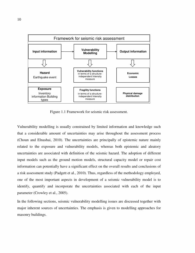
direct economic losses (Figure 1.1). Earthquake induced hazards such as liquefaction and
landslides are not considered in this study.
10
Vulnerability Modelling
Hazard
Earthquake event
Exposure
Inventory information Building
types
Vulnerability functions in terms of a structure-independent Intensity
measure
Input information Output information
EconomicLosses
Fragility functions
in terms of a structure-independent Intensity
measure
Physical damage distribution
Framework for seismic risk assessment
Figure 1.1 Framework for seismic risk assessment.
Vulnerability modelling is usually constrained by limited information and knowledge such
that a considerable amount of uncertainties may arise throughout the assessment process
(Choun and Elnashai, 2010). The uncertainties are principally of epistemic nature mainly
related to the exposure and vulnerability models, whereas both epistemic and aleatory
uncertainties are associated with definition of the seismic hazard. The adoption of different
input models such as the ground motion models, structural capacity model or repair cost
information can potentially have a significant effect on the overall results and conclusions of
a risk assessment study (Padgett et al., 2010). Thus, regardless of the methodology employed,
one of the most important aspects in development of a seismic vulnerability model is to
identify, quantify and incorporate the uncertainties associated with each of the input
parameter (Crowley et al., 2005).
In the following sections, seismic vulnerability modelling issues are discussed together with
major inherent sources of uncertainties. The emphasis is given to modelling approaches for
masonry buildings.
11
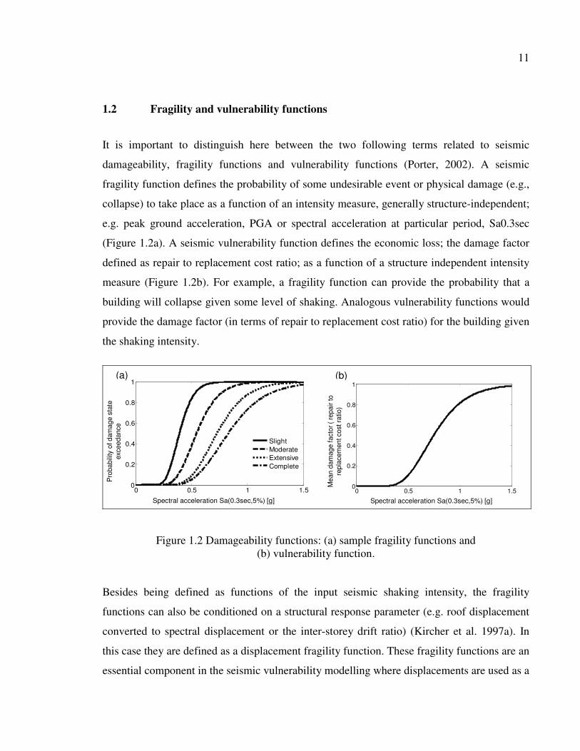
1.2 Fragility and vulnerability functions
It is important to distinguish here between the two following terms related to seismic
damageability, fragility functions and vulnerability functions (Porter, 2002). A seismic
fragility function defines the probability of some undesirable event or physical damage (e.g.,
collapse) to take place as a function of an intensity measure, generally structure-independent;
e.g. peak ground acceleration, PGA or spectral acceleration at particular period, Sa0.3sec
(Figure 1.2a). A seismic vulnerability function defines the economic loss; the damage factor
defined as repair to replacement cost ratio; as a function of a structure independent intensity
measure (Figure 1.2b). For example, a fragility function can provide the probability that a
building will collapse given some level of shaking. Analogous vulnerability functions would
provide the damage factor (in terms of repair to replacement cost ratio) for the building given
the shaking intensity.
0 0.5 1 1.50
0.2
0.4
0.6
0.8
1
Sa(0.3sec,5%) [g]
P(D
S >
dsi
)
SlightModerateExtensiveComplete
M = 7 ,R=20kmSoil-C
0 0.5 1 1.50
0.2
0.4
0.6
0.8
1
Sa(0.3sec,5%) [g]
MD
F
M = 7 , R=20kmSoil-C
(a) (b)
Spectral acceleration Sa(0.3sec,5%) [g] Spectral acceleration Sa(0.3sec,5%) [g]
Pro
babi
lity
of d
amag
e st
ate
exce
edan
ce
Mea
n da
mag
e fa
ctor
( re
pair
to
repl
acem
ent c
ost r
atio
)
Figure 1.2 Damageability functions: (a) sample fragility functions and (b) vulnerability function.
Besides being defined as functions of the input seismic shaking intensity, the fragility
functions can also be conditioned on a structural response parameter (e.g. roof displacement
converted to spectral displacement or the inter-storey drift ratio) (Kircher et al. 1997a). In
this case they are defined as a displacement fragility function. These fragility functions are an
essential component in the seismic vulnerability modelling where displacements are used as a

12
measure of the extent of seismic induced damage. This type of functions is discussed in more
details in the subsequent sections.
Fragility and vulnerability functions can be obtained from empirical, expert opinion,
analytical models or any combinations of these models (hybrid approach) (Rossetto and
Elnashai, 2005). Whatever the method used to predict the seismic damageability, they all
contain uncertainties in the assessment procedures and data used. They include measurement
uncertainty related to the observations, inconsistency in the quality of the analysis and
database, variability of the ground motion, uncertainty in the judgment of experts,
uncertainty due to simplification of models for the strength and stiffness of structural
materials and components, uncertainties in seismic demand and capacity of structures due to
variations of their geometry and material properties, and uncertainty in the definition of the
damage states.
Because of the scarcity of observational damage data in regions of moderate seismicity such
as Eastern Canada and the subjectivity of judgmental damage data, recent vulnerability
modelling is focused mainly on analytical methods. Analytical methods rely on structural
modelling and analytical evaluation of the likelihood of damage by earthquakes of a given
intensity, as well as on consideration of uncertainty relative to ground motion and structural
parameters. Analytical methods; however, require significant computational effort and
generally there are some choices in each component of the methodology. The components of
analytical modelling are discussed in detail in the next sections.
1.3 Analytical vulnerability modelling and uncertainty quantification
Analytical approaches for generating fragility and vulnerability functions for a particular
building class comprise four general steps: hazard analysis, structural analysis, damage
analysis and loss analysis (Porter, 2002) (Figure 1.3). The building class is established in
accordance with similarities in the structural system; height and material of construction. A
structural analysis is performed on a structural model built for that building class to estimate
the structural response to the input ground motion corresponding to various levels of
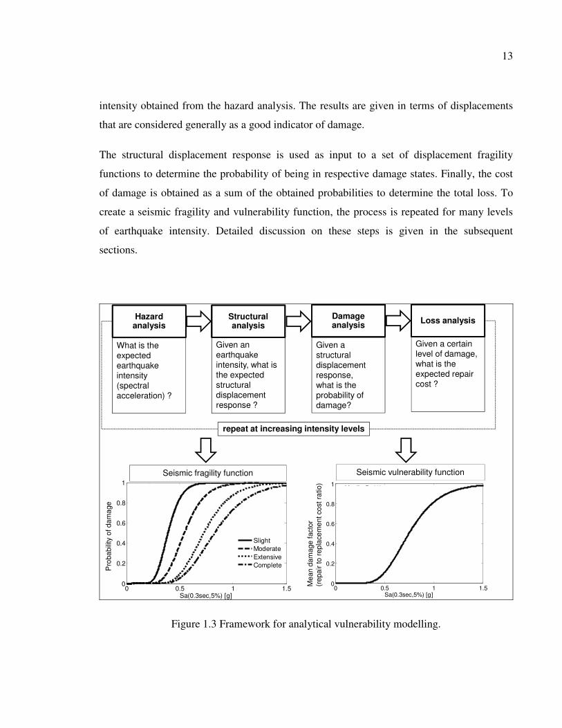
13
intensity obtained from the hazard analysis. The results are given in terms of displacements
that are considered generally as a good indicator of damage.
The structural displacement response is used as input to a set of displacement fragility
functions to determine the probability of being in respective damage states. Finally, the cost
of damage is obtained as a sum of the obtained probabilities to determine the total loss. To
create a seismic fragility and vulnerability function, the process is repeated for many levels
of earthquake intensity. Detailed discussion on these steps is given in the subsequent
sections.
0 0.5 1 1.50
0.2
0.4
0.6
0.8
1
Sa(0.3sec,5%) [g]
P(D
S >
dsi
)
SlightModerateExtensiveComplete
M = 7 ,R=20kmSoil-C
11
Given an earthquake intensity, what is the expected structural displacement response ?
Damage analysis
Hazard analysis
Structural analysis
repeat at increasing intensity levels
Seismic fragility function
What is the expected earthquake intensity (spectral acceleration) ?
Given a structural displacement response, what is the probability of damage?
Given a certain level of damage, what is the expected repair cost ?
0 0.5 1 1.50
0.2
0.4
0.6
0.8
1
Sa(0.3sec,5%) [g]
MD
F
M = 7 , R=20kmSoil-C
Seismic vulnerability function
Loss analysisM
ean
dam
age
fact
or
(rep
air
to r
epla
cem
ent c
ost r
atio
)
Pro
babi
lity
of d
amag
e
Figure 1.3 Framework for analytical vulnerability modelling.
14
It should be noted that representing fragility and vulnerability functions in terms of a
structure-independent intensity measure provides rapid assessment of damage and losses in
the framework of regional scale risk assessment for several classes of buildings with reduced
computational time. This is related to the fact that fragility functions can be directly used
with the seismic hazard output, typically presented in terms of a structure-independent
intensity measure.
There are many different approaches associated to each step of the analytical vulnerability
modelling. The ground motion, for example, can be characterized in terms of response
spectra or in terms of acceleration time histories. The nonlinear structural analysis can either
be static or dynamic; it can be performed including an equivalent single degree of freedom
(ESDOF) or a multi-degree of freedom system (MDOF). The damage analysis can either be
based on global structural displacement or local inter-storey drift demands. As mentioned in
the introductory part, each of the steps involves uncertainty. The major sources of
uncertainties in the vulnerability modelling are related: details of the ground motion for a
given intensity level, structural properties such as damping, and force-deformation
behaviour, damage state definition and repair costs conditioned on damage. A good
vulnerability modelling practice should address the important sources of uncertainty.
The input structural parameters to an analytical vulnerability model depend on the selected
structural analysis method. For example, if a nonlinear static analysis method is selected, a
capacity curve, describing the nonlinear force-deformation characteristics for the considered
ESDOF approximation of the building, should be provided along with a set of displacement
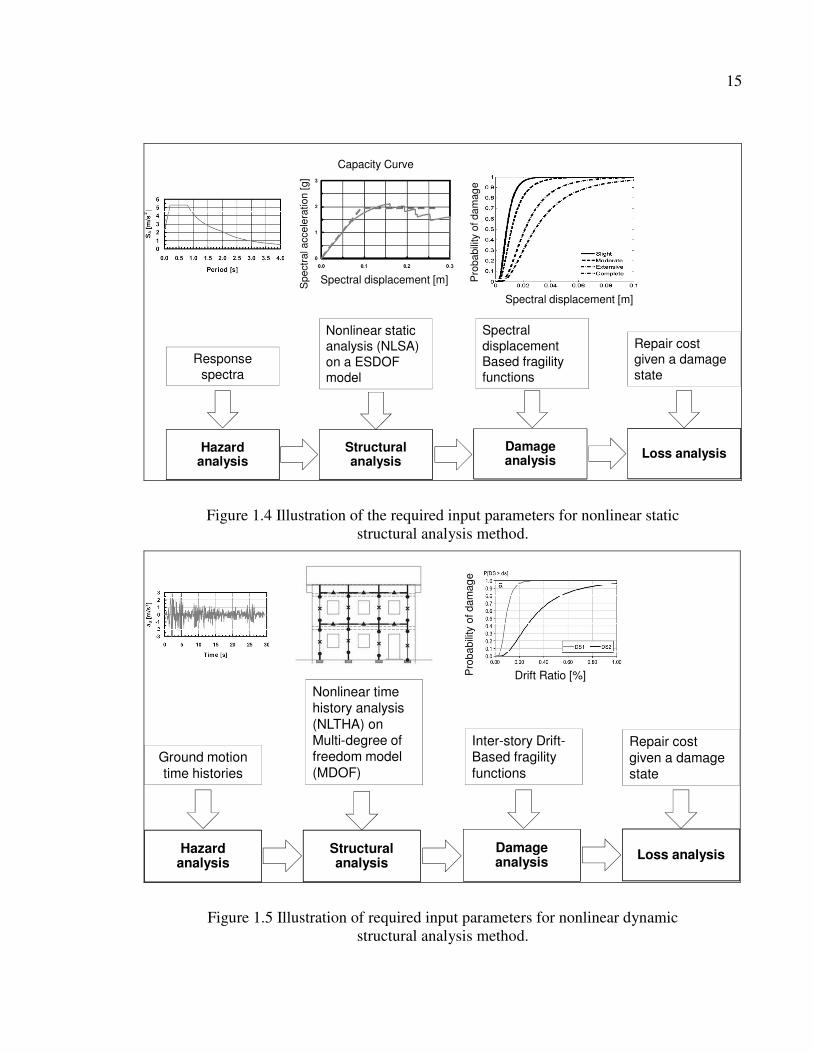
fragility functions in terms of spectral displacement response (Figure 1.4). This approach is
adopted in the vulnerability model of the North American loss estimation tool Hazus (FEMA,
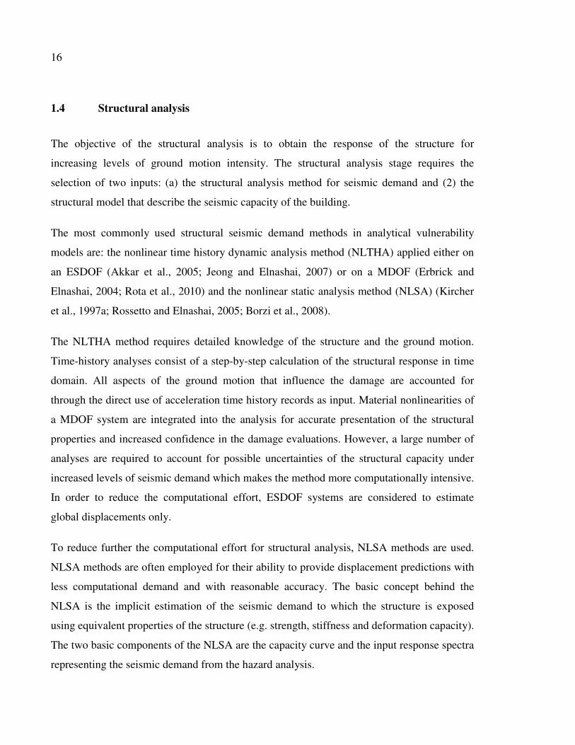
2003) and the European Earthquake Loss Estimation Routine ELER (Erdik et al., 2010). If a
nonlinear dynamic analysis is selected, a MDOF model of the structure should be provided
along with an inter-storey drift response fragility functions (Porter, 2002) (Figure 1.5).
15
Nonlinear static analysis (NLSA) on a ESDOF model
Damage analysis
Hazard analysis
Structural analysis
Response spectra
Spectral displacement Based fragility functions
Repair cost given a damage state
Loss analysis
Pro
babi
lity
of d
amag
e
Spectral displacement [m]
Capacity Curve
Spectral displacement [m]Spe
ctra
l acc
eler
atio
n [g
]
Figure 1.4 Illustration of the required input parameters for nonlinear static structural analysis method.
Nonlinear time history analysis (NLTHA) onMulti-degree of freedom model (MDOF)
Damage analysis
Hazard analysis
Structural analysis
Ground motion time histories
Inter-story Drift-Based fragility functions
Repair cost given a damage state
Loss analysis
Drift Ratio [%]Pro
babi
lity
of d
amag
e
Figure 1.5 Illustration of required input parameters for nonlinear dynamic structural analysis method.
16
1.4 Structural analysis
The objective of the structural analysis is to obtain the response of the structure for
increasing levels of ground motion intensity. The structural analysis stage requires the
selection of two inputs: (a) the structural analysis method for seismic demand and (2) the
structural model that describe the seismic capacity of the building.
The most commonly used structural seismic demand methods in analytical vulnerability
models are: the nonlinear time history dynamic analysis method (NLTHA) applied either on
an ESDOF (Akkar et al., 2005; Jeong and Elnashai, 2007) or on a MDOF (Erbrick and
Elnashai, 2004; Rota et al., 2010) and the nonlinear static analysis method (NLSA) (Kircher
et al., 1997a; Rossetto and Elnashai, 2005; Borzi et al., 2008).
The NLTHA method requires detailed knowledge of the structure and the ground motion.
Time-history analyses consist of a step-by-step calculation of the structural response in time
domain. All aspects of the ground motion that influence the damage are accounted for
through the direct use of acceleration time history records as input. Material nonlinearities of
a MDOF system are integrated into the analysis for accurate presentation of the structural
properties and increased confidence in the damage evaluations. However, a large number of
analyses are required to account for possible uncertainties of the structural capacity under
increased levels of seismic demand which makes the method more computationally intensive.
In order to reduce the computational effort, ESDOF systems are considered to estimate
global displacements only.
To reduce further the computational effort for structural analysis, NLSA methods are used.
NLSA methods are often employed for their ability to provide displacement predictions with
less computational demand and with reasonable accuracy. The basic concept behind the
NLSA is the implicit estimation of the seismic demand to which the structure is exposed
using equivalent properties of the structure (e.g. strength, stiffness and deformation capacity).
The two basic components of the NLSA are the capacity curve and the input response spectra
representing the seismic demand from the hazard analysis.

17
NLSA requires less computational time and effort than the NLTHA, which offers a
considerable advantage in vulnerability modelling of populations of buildings. The most
commonly used NLSA methods in vulnerability modelling are the capacity spectrum method
(CSM) (Mahaney et al., 1993; ATC 40, 1996) which is the structural analysis method in
Hazus (FEMA, 2003) and ELER (Erdik et al., 2010) and the displacement coefficient method
(DCM) presented in FEMA356 (FEMA, 2000); FEMA440 (FEMA, 2005) and ASCE-41
(ASCE, 2007).
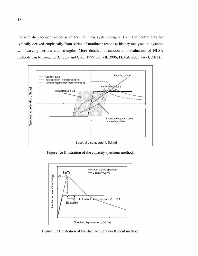
CSM is based on equivalent linearization approach in which the maximum displacement of a
SDOF system can be estimated by the elastic response of a system with increased effective
period and damping than the original. The CSM assumes that the equivalent damping of the
system is proportional to the area enclosed by the capacity curve (Figure 1.6). The equivalent
period is assumed to be the secant period at which the seismic demand, reduced by the
additional damping due to the nonlinear response, intersects the capacity curve. Since the
equivalent period and damping are both functions of the displacement, the solution to
determine the maximum inelastic displacement (i.e., performance point) is iterative. Another
version of the CSM is proposed in FEMA440 (FEMA, 2005) in which the equivalent period
of the equivalent linear system is obtained from equivalent stiffness that lies between the
initial stiffness and the secant stiffness of the inelastic system. The equivalent period and
equivalent damping were derived from SDOF systems subjected to a series of earthquake
records by finding the optimal pair of equivalent period and equivalent damping that
minimizes the error between the response of the equivalent linear system and the actual
response of the inelastic system. Another variant of the CSM method is based on the inelastic
response spectrum instead of the over damped response spectrum of an equivalent linear
system (Chopra and Goel, 1999; Fajfar, 1999). According to this method, the elastic response
spectrum is modified using a reduction factor (R�) that is a function of the ductility (�)
demand and the period of the elastic system (T), typically defined as R�-�-T relationships.
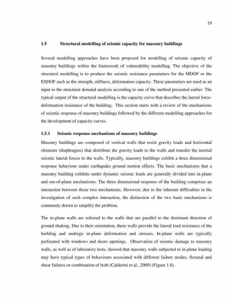
The DCM is a displacement modification procedure which estimates the total maximum
displacement of the system by multiplying the elastic response based on the initial linear
properties and damping, by a series of coefficients C1 and C2 to generate an estimate of the
18
inelastic displacement response of the nonlinear system (Figure 1.7). The coefficients are
typically derived empirically from series of nonlinear response history analyses on systems
with varying periods and strengths. More detailed discussion and evaluation of NLSA
methods can be found in (Chopra and Goel, 1999; Powell, 2006; FEMA, 2005; Goel, 2011).
-0.8
-0.6
-0.4
-0.2
0
0.2
0.4
0.6
0.8
-0.04 -0.03 -0.02 -0.01 0 0.01 0.02 0.03 0.04
Spe
ctra
l acc
eler
atio
n, S
a [g
]
Spectral displacement, Sd [m]
Capacity curveInput spectrum for elastic dampingDemand spectrum for effective damping
(Sd ,Sa,, �eff)Performance point
Full hysteresis area
Reduced hysteresis area due to degradation
Effective period
Figure 1.6 Illustration of the capacity spectrum method.
0.00
0.10
0.20
0.30
0.40
0.50
0.60
0.70
0 0.01 0.02 0.03 0.04
Spe
ctra
l acc
eler
atio
n, S
a [g
]
Spectral displacement, Sd [m]
Input elastic spectrumCapacity CurveSa(To)
Sd inelastic = Sd elastic * C1 * C2Sd elastic
Figure 1.7 Illustration of the displacement coefficient method.
19
1.5 Structural modelling of seismic capacity for masonry buildings
Several modelling approaches have been proposed for modelling of seismic capacity of
masonry buildings within the framework of vulnerability modelling. The objective of the
structural modelling is to produce the seismic resistance parameters for the MDOF or the
ESDOF such as the strength, stiffness, deformation capacity. These parameters are used as an
input to the structural demand analysis according to one of the method presented earlier. The
typical output of the structural modelling is the capacity curve that describes the lateral force-
deformation resistance of the building. This section starts with a review of the mechanisms
of seismic response of masonry buildings followed by the different modelling approaches for
the development of capacity curves.
1.5.1 Seismic response mechanisms of masonry buildings
Masonry buildings are composed of vertical walls that resist gravity loads and horizontal
elements (diaphragms) that distribute the gravity loads to the walls and transfer the inertial
seismic lateral forces to the walls. Typically, masonry buildings exhibit a three dimensional
response behaviour under earthquake ground motion effects. The basic mechanisms that a
masonry building exhibits under dynamic seismic loads are generally divided into in-plane
and out-of-plane mechanisms. The three dimensional response of the building comprises an
interaction between those two mechanisms. However, due to the inherent difficulties in the
investigation of such complex interaction, the distinction of the two basic mechanisms is
commonly drawn to simplify the problem.
The in-plane walls are referred to the walls that are parallel to the dominant direction of
ground shaking. Due to their orientation, these walls provide the lateral load resistance of the
building and undergo in-plane deformation and stresses. In-plane walls are typically
perforated with windows and doors openings. Observation of seismic damage to masonry
walls, as well as of laboratory tests, showed that masonry walls subjected to in-plane loading
may have typical types of behaviours associated with different failure modes, flexural and
shear failures or combination of both (Calderini et al., 2009) (Figure 1.8).
20
The flexural failure (Figure 1.8a) occurs when the horizontal load produces tensile flexural
cracking at the corners and the wall begins to behave as a nearly rigid body rotating about the
toe and with progressively increasing cracks oriented towards the more compressed corners
(crushing). The diagonal shear failure (Figure 1.8b) is typically characterized by the
formation of a diagonal crack, which usually develops at the centre of the wall and then
propagates towards the corners. The crack progresses generally through the mortar joints in
the case of a regular masonry pattern, but it can also go through the blocks. Another failure
mode that may occur is the sliding shear failure (Figure 1.8c), where failure is attained with
sliding on a horizontal bed joint plane, usually located at one of the extremities of the wall.
However, this failure is only possible for very squat walls. The most commonly observed in-
plane failure mechanism from post-earthquake damage surveys is the diagonal cracking shear
failure especially in old brick and stone masonry building (Figure 1.9; Tomazevic, 1999;
Lutman and Tomazevic; 2002).
The occurrence of different failure modes depends on several parameters: geometry of the
wall; boundary conditions; acting axial load; mechanical characteristics of the masonry
constituents (compression and shear strength of masonry); masonry geometrical
characteristics (block aspect ratio, masonry pattern). It should be noted that it is not easy to
distinguish the occurrence of a specific type of mechanism, since two or more failure
mechanisms may occur with interactions between them. Flexural failure tends to prevail in
slender walls, while diagonal cracking tends to prevail in moderate slender walls over flexure
and bed joint sliding for increasing levels of vertical compression. On the other hand,
diagonal cracking propagating through blocks tends to prevail over diagonal cracking
propagating through mortar joints for increasing levels of vertical compression and for
increasing ratios between mortar and block strengths.
21
Toe crushing
(a) (b) (c)
Figure 1.8 In-plane failure mechanisms of masonry walls: (a) flexural failure, (b) diagonal shear failure and (c) sliding shear failure
Taken from Calderini et al. (2009)
(a) (b)
Figure 1.9 Photographs illustrating typical diagonal cracking damage for: (a) a stone masonry buildings and (b) a brick masonry building Taken from Lutman and Tomazevic (2002)
The force-deformation hysteresis behaviour and the energy dissipation capacity of masonry
walls under in-plane cyclic loading are influenced by the failure mechanism. A typical
flexural response is shown in Figure 1.10a, where large displacements can be obtained
without significant loss in strength, especially when the mean axial load is low compared to
the compressive strength of masonry. Limited hysteretic energy dissipation is observed, with
negligible strength degradation under load reversals. Figure 1.10b shows typical hysteresis
behaviour of walls with diagonal cracking shear mechanism where the response is
22
characterized by higher energy dissipation compared to rocking mechanisms but by rather
rapid strength and stiffness degradation.
(a) (b)
Figure 1.10 Force-deformation hysteresis behaviour of masonry walls: (a) flexural rocking failure mechanism and (b) shear failure mechanism with diagonal cracking
Taken from Magenes and Calvi (1997)
Walls that are perpendicular to the direction of ground shaking are typically vulnerable to the
out-of-plane damage. The out-of-plane wall works like a thin plate supported on the edges
adjacent to the in-plane walls. The boundary element of the out-of-plane wall is the
connections with the floor systems. During an earthquake, the out-of-plane wall vibrates
under the seismic force induced by its own mass and the forces transferred from floor and in-
plane walls. The vibration and the associated bending deformation may lead to cracking and
out-of-plane collapse of the wall.
When not properly connected to floors and in-plane walls, the out-of-plane masonry wall can
become unstable and may collapse under out-of-plane vibrations (Bruneau, 1994). However,
if the connections between the wall and the floors have sufficient strength, the out-of-plane
behaviour is not critical and the seismic response is governed by the in-plane walls
(Tomazevic, 1999).
23
1.5.2 Capacity modelling methods
Analytical methods that are used to predict the seismic capacity of masonry buildings
represented by; either a MDOF or an ESDOF system, can be classified into two main
categories: simulation-based methods (Rossetto and Elnashai, 2005; Erberik, 2008; Rota et
al., 2010) and mechanics-based methods (Oropeza et al., 2010, Lang, 2002, Borzi et al.,
2008; Restrepo-Velez, 2003). The simulation based methods uses detailed structural models.
The mechanics based methods apply simplified structural mechanics models to develop the
strength, stiffness and deformation parameters of the building.
The detailed structural models used in the simulation based methods can be subdivided into:
micro-scale models and macro-scale models (Figure 1.11; Calderini et al., 2009). In the
micro-scale models, the structure is discretized into finite-elements with inelastic constitutive
models at the material level. In the macro-scale models, the structure is discretized into an
equivalent frame model with main structural components: masonry piers and spandrels are
modelled with force-deformation relationship at the structural member level. The micro-scale
models require significantly high computational resources and experience and their use is
mainly limited to the prediction of the behaviour of individual structural components (piers
or spandrels) and confirmation of the accuracy of the macro-models on the structural level.
The simulation-based methods require detailed knowledge of the inelastic behaviour of the
material, large amount of input parameters and consequently longer computational time
which would be unsuitable for vulnerability assessment of large number of structures.
Therefore, simulation-based methods are commonly limited to vulnerability modelling of a
single representative building (Rota et al., 2010).
24
Figure 1.11 Detailed structural models: (a) micro-scale model using finite elements and (b) macro-scale model using the equivalent frame idealization
Taken from Calderini et al. (2009)
The mechanics based methods apply simplified structural mechanics principles to develop
the strength, stiffness and deformation parameters of single masonry walls and combine them
to produce the capacity curve of the building (Figure 1.12). Tomazevic (1999) and Lang
(2002) have shown that the application of simplified mechanical models provided good
approximation of the global system capacity when compared with experimental results of
shaking table tests conducted on several scaled models of masonry buildings. Such
simplification reduces the computation time and more importantly idealizes the system with
less number of parameters which is highly desirable when conducting regional scale
vulnerability modelling.
25
x
YResisting walls(facade walls)in the X direction
Top displacement [m]
V, shear force [kN]
Capacity curve for wall-1
Capacity curve for all wallsVbase shear
Fire walls
.Displacement shape
ElasticDisp.
InelasticDisp.
Capacity curve for wall-2
Capacity curve for wall-3
Wall-1 Wall-2 Wall-3
Figure 1.12 Illustration of a capacity curve of a masonry building using mechanics-based models.
The capacity curves developed by either of the methods presented above can be converted to
a simplified ESDOF system with global capacity parameters (stiffness, strength and
deformation capacity). The ESDOF system is more suitable for seismic demand analysis for
population of buildings. This approach has the advantage of reducing the computational
effort to practical level and allows conducting large amount of analysis for many structures
and the assessment of uncertainties in such models.
The base shear – roof displacement relationships are typically converted to standard capacity
curves defined by the spectral acceleration - spectral displacement relationship (Fajfar,
2000). The conversion method from MDOF to ESDOF system is presented as follows:
*
*
*
2
.
.
.
d
a
i i
i i
S
VS
m
m m
m
m
ϕ
ϕ
Δ=
Γ
=Γ
=
Γ =
�
�
(1.1)

26
Where Sd and Sa are the spectral displacement and spectral acceleration of the ESDOF
system, respectively; � is the top displacement for the MDOF capacity curve, m* is the
equivalent mass of the ESDOF system, mi is the concentrated mass of the floors (the mass of
the walls is divided between the two levels above and below the i-th floor level, �i is the first
mode displacement at the i-th floor level normalized such that the first mode displacement at
the top story � =1.0; � is modal participation factor that control the transformation from the
MDOF to the ESDOF (Figure 1.13a). The above conversion has the advantage to allow a
direct comparison with the seismic demand represented with response spectra (Figure 1.13b).
(a)
Heff
H
-
(b)
0
100
200
300
400
0 0.01 0.02 0.03 0.04 0.05 0.06
Bas
e sh
ear
V[k
N]
Top Displacement � [m]
0.00
0.05
0.10
0.15
0.20
0.25
0 0.01 0.02 0.03 0.04 0.05 0.06
Spe
ctra
l acc
eler
atio
nS
a =
V/(
m* �)
[g]
Spectral Displacement Sd = (�/�) [m]
Figure 1.13 Illustration of the conversion of the MDOF system to an ESDOF: (a) the mode shape and mass distribution and (b) the conversion of the
capacity curve to the spectral acceleration-displacement domain.

27
1.6 Damage analysis
Building performance can be measured by mechanical quantities related to the physical
condition of the building following an earthquake. In evaluating structural performance, it is
of interest that these mechanical quantities do not exceed certain threshold levels defined as
damage states. A damage state represent the condition where damage occurred has a direct
impact on building use after an earthquake and on the expected losses. For example, a
complete damage state corresponds to the demolition of the building.
Well-defined and realistic damage states thresholds are essential for vulnerability modelling.
Damage states thresholds are identified using quantitative parameters that correlate best with
damage. Inter-story drift ratio and building roof displacement are widely used parameters for
damage assessment of structures and are used to develop displacement fragility functions
taking into account inherent uncertainties.
Damage state thresholds for masonry buildings are typically identified based on experimental
drift ratios of masonry walls tested under cyclic loading (Borzi et al., 2008; Restrepo-Velez,
2003, Ruiz-García and Negrete, 2009; Bosiljkov et al., 2010). Figure 1.14 shows an example
for the identification of drift thresholds corresponding to flexural cracking (Hf), shear
cracking (Hdt), maximum shear strength (Hmax), and ultimate deformation at 20% loss of
strength (H�max). They are considered as respective damage thresholds for the slight,
moderate, extensive, and complete damage states. Based on several test results, the damage
state thresholds can be represented in a probabilistic format as a fragility function (Figure
1.15). Typically, the fragility functions are represented by a lognormal probability
distribution with a median value and a standard deviation. Lognormal distribution is typically
used since it has shown a good fit for structural damage distribution (Wen et al., 2004).

28
Figure 1.14 Identification of the drift thresholds that corresponds to reaching a specific damage state
Taken from Bosiljkov et al., (2010)
DS1
DS2
Figure 1.15 Example of a drift-based fragility functions for confined masonry walls Taken from Ruiz-García and Negrete (2009)
For an ESDOF idealization of the building, the drift-based damage fragility functions can
also be converted to spectral displacements fragility functions (Figure 1.16) In this case, they
can be convolved directly with the results of the inelastic spectral displacement response
from structural analysis (Kircher et al., 1997a, FEMA, 2003, Erdik et al., 2010).
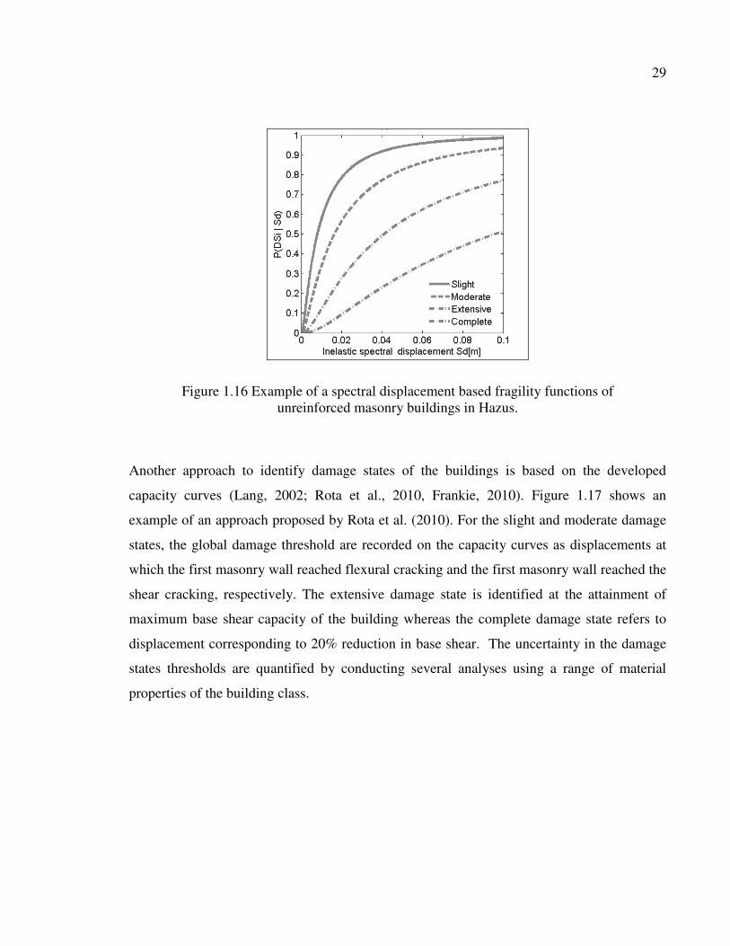
29
Figure 1.16 Example of a spectral displacement based fragility functions of unreinforced masonry buildings in Hazus.
Another approach to identify damage states of the buildings is based on the developed
capacity curves (Lang, 2002; Rota et al., 2010, Frankie, 2010). Figure 1.17 shows an
example of an approach proposed by Rota et al. (2010). For the slight and moderate damage
states, the global damage threshold are recorded on the capacity curves as displacements at
which the first masonry wall reached flexural cracking and the first masonry wall reached the
shear cracking, respectively. The extensive damage state is identified at the attainment of
maximum base shear capacity of the building whereas the complete damage state refers to
displacement corresponding to 20% reduction in base shear. The uncertainty in the damage
states thresholds are quantified by conducting several analyses using a range of material
properties of the building class.
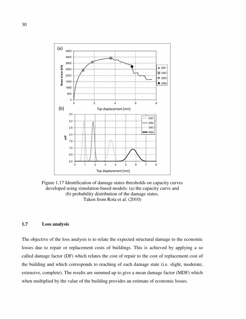
30
Top displacement [mm]
Top displacement [mm]
���
���
Figure 1.17 Identification of damage states thresholds on capacity curves developed using simulation-based models: (a) the capacity curve and
(b) probability distribution of the damage states. Taken from Rota et al. (2010)
1.7 Loss analysis
The objective of the loss analysis is to relate the expected structural damage to the economic
losses due to repair or replacement costs of buildings. This is achieved by applying a so
called damage factor (DF) which relates the cost of repair to the cost of replacement cost of
the building and which corresponds to reaching of each damage state (i.e. slight, moderate,
extensive, complete). The results are summed up to give a mean damage factor (MDF) which
when multiplied by the value of the building provides an estimate of economic losses.
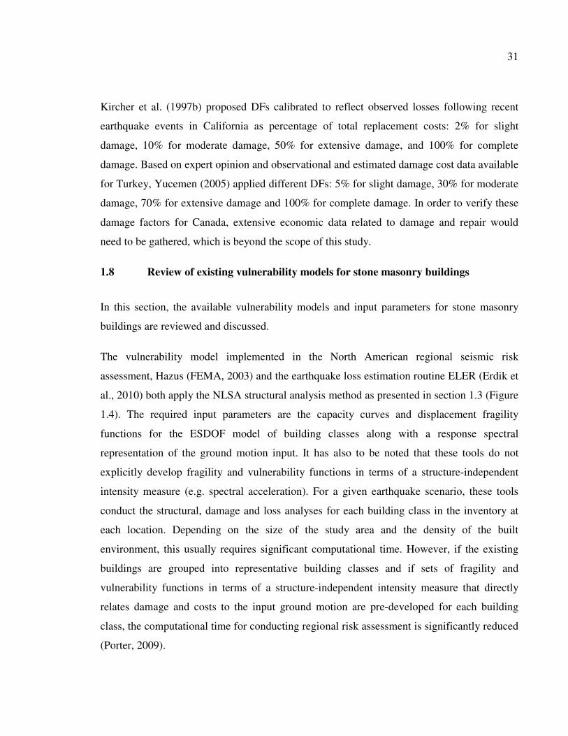
31
Kircher et al. (1997b) proposed DFs calibrated to reflect observed losses following recent
earthquake events in California as percentage of total replacement costs: 2% for slight
damage, 10% for moderate damage, 50% for extensive damage, and 100% for complete
damage. Based on expert opinion and observational and estimated damage cost data available
for Turkey, Yucemen (2005) applied different DFs: 5% for slight damage, 30% for moderate
damage, 70% for extensive damage and 100% for complete damage. In order to verify these
damage factors for Canada, extensive economic data related to damage and repair would
need to be gathered, which is beyond the scope of this study.
1.8 Review of existing vulnerability models for stone masonry buildings
In this section, the available vulnerability models and input parameters for stone masonry
buildings are reviewed and discussed.
The vulnerability model implemented in the North American regional seismic risk
assessment, Hazus (FEMA, 2003) and the earthquake loss estimation routine ELER (Erdik et
al., 2010) both apply the NLSA structural analysis method as presented in section 1.3 (Figure
1.4). The required input parameters are the capacity curves and displacement fragility
functions for the ESDOF model of building classes along with a response spectral
representation of the ground motion input. It has also to be noted that these tools do not
explicitly develop fragility and vulnerability functions in terms of a structure-independent
intensity measure (e.g. spectral acceleration). For a given earthquake scenario, these tools
conduct the structural, damage and loss analyses for each building class in the inventory at
each location. Depending on the size of the study area and the density of the built
environment, this usually requires significant computational time. However, if the existing
buildings are grouped into representative building classes and if sets of fragility and
vulnerability functions in terms of a structure-independent intensity measure that directly
relates damage and costs to the input ground motion are pre-developed for each building
class, the computational time for conducting regional risk assessment is significantly reduced
(Porter, 2009).
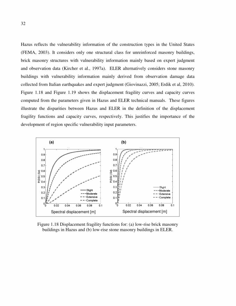
32
Hazus reflects the vulnerability information of the construction types in the United States
(FEMA, 2003). It considers only one structural class for unreinforced masonry buildings,
brick masonry structures with vulnerability information mainly based on expert judgment
and observation data (Kircher et al., 1997a). ELER alternatively considers stone masonry
buildings with vulnerability information mainly derived from observation damage data
collected from Italian earthquakes and expert judgment (Giovinazzi, 2005; Erdik et al, 2010).
Figure 1.18 and Figure 1.19 shows the displacement fragility curves and capacity curves
computed from the parameters given in Hazus and ELER technical manuals. These figures
illustrate the disparities between Hazus and ELER in the definition of the displacement
fragility functions and capacity curves, respectively. This justifies the importance of the
development of region specific vulnerability input parameters.
Spectral displacement [m] Spectral displacement [m]
(a) (b)
Figure 1.18 Displacement fragility functions for: (a) low-rise brick masonry buildings in Hazus and (b) low-rise stone masonry buildings in ELER.
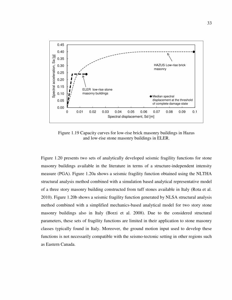
33
0.00
0.05
0.10
0.15
0.20
0.25
0.30
0.35
0.40
0.45
0 0.01 0.02 0.03 0.04 0.05 0.06 0.07 0.08 0.09 0.1
Spe
ctra
l acc
eler
atio
n, S
a [g
]
Spectral displacement, Sd [m]
ELER low-rise stonemasonry buildings
HAZUS Low-rise brick masonry
Median spectral displacement at the threshold of complete damage state
Figure 1.19 Capacity curves for low-rise brick masonry buildings in Hazus and low-rise stone masonry buildings in ELER.
Figure 1.20 presents two sets of analytically developed seismic fragility functions for stone
masonry buildings available in the literature in terms of a structure-independent intensity
measure (PGA). Figure 1.20a shows a seismic fragility function obtained using the NLTHA
structural analysis method combined with a simulation based analytical representative model
of a three story masonry building constructed from tuff stones available in Italy (Rota et al.
2010). Figure 1.20b shows a seismic fragility function generated by NLSA structural analysis
method combined with a simplified mechanics-based analytical model for two story stone
masonry buildings also in Italy (Borzi et al. 2008). Due to the considered structural
parameters, these sets of fragility functions are limited in their application to stone masonry
classes typically found in Italy. Moreover, the ground motion input used to develop these
functions is not necessarily compatible with the seismo-tectonic setting in other regions such
as Eastern Canada.
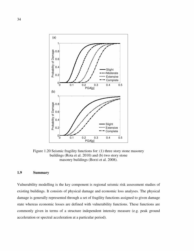
34
0 0.1 0.2 0.3 0.4 0.50
0.2
0.4
0.6
0.8
1
PGA[g]
Pro
babi
lity
of D
amag
e
SlightExtensiveComplete
0 0.1 0.2 0.3 0.4 0.50
0.2
0.4
0.6
0.8
1
PGA[g]
Pro
babi
lity
of D
amag
e
SlightModerateExtensiveComplete
(a)
(b)
Figure 1.20 Seismic fragility functions for: (1) three story stone masonry buildings (Rota et al. 2010) and (b) two story stone
masonry buildings (Borzi et al. 2008).
1.9 Summary
Vulnerability modelling is the key component is regional seismic risk assessment studies of
existing buildings. It consists of physical damage and economic loss analyses. The physical
damage is generally represented through a set of fragility functions assigned to given damage
state whereas economic losses are defined with vulnerability functions. These functions are
commonly given in terms of a structure independent intensity measure (e.g. peak ground
acceleration or spectral acceleration at a particular period).

35
Analytical approaches for vulnerability modelling are typically adopted in the regions of
moderate seismicity where damage data from past earthquakes are scarce. Despite the high
vulnerability of stone masonry buildings, literature review revealed less research is focused
on regional seismic vulnerability modelling of these buildings compared to other structural
types, e.g. brick masonry and concrete structures.
Analytical approaches for generating fragility and vulnerability functions for a particular
building class comprise several steps. The building class is established in accordance with
similarities in the structural system; height and material of construction, along with ground
motions corresponding to various levels of intensity obtained from the hazard analysis. A
structural analysis is performed on a structural model built for that building class to estimate
the structural response to the input ground motion. The results are given in terms of
displacements that are considered generally as a good indicator of damage. The structural
displacement response is used as input to a set of displacement fragility functions to
determine the probability of being in respective damage states. Finally, the cost of damage is
obtained as a sum of the obtained probabilities to determine the total loss. To create a
seismic fragility and vulnerability function, the process is repeated for many levels of
earthquake intensity.
Each of the vulnerability modelling steps involves uncertainty. The major sources of
uncertainties in the vulnerability modelling are related to: details of the ground motion,
structural seismic capacity, damage state definition and repair costs. A good vulnerability
modelling practice should address the important sources of uncertainty and investigate their
sensitivity to the results.
The review of literature showed that existing vulnerability tools in North America does not
consider the stone masonry building classes subjected to Eastern Canada ground motions.
Therefore, sets of seismic fragility and vulnerability functions for these buildings need to be
developed in order to adequately quantify their seismic risk.
36
This study will focus on the development of probabilistic assessment tools for seismic
vulnerability of stone masonry buildings. These tools will be applied to assess the seismic
risk of stone masonry building and other building classes at Old Quebec City. A framework
that considers and quantifies different sources of uncertainties will be introduced. In the
following chapters, these research issues will be addressed in further details.

CHAPTER 2
DISPLACEMENT BASED FRAGILITY ANALYSIS
2.1 Introduction
The objective of this chapter is to introduce a simplified analytical-based fragility analysis
procedure with systematic treatment of uncertainties for development of displacement based
fragility functions for typical stone masonry buildings in Old Quebec City. The applied
procedure comprises: (1) inventory of the existing buildings, (2) probabilistic displacement-
based damage model, (3) probabilistic capacity model, (4) probabilistic seismic demand
model. The resulting fragility functions are compared with those implicit in Hazus (FEMA,
2003) and ELER (Erdik et al., 2010) in order to assess differences and the potential
disparities in damage estimates. The comparison are conducted in terms of probability of
reaching a given damage state.
2.2 Analytical displacement fragility functions
Analytical displacement fragility functions are usually given in the form of lognormal
distribution of the probability of being in or exceeding a given damage state for structural
response parameter (e.g., spectral inelastic displacement demand). The conditional
probability of reaching a particular damage state, DS , given the spectral displacement dS , is
defined by the following equation (Kircher et al., 1997a):
[ ],
2 2
1| ln
( , )
dd
d DSDS
DS C D T
SP DS S
S
CONV
β
β β β β
� �� �= Φ � �
� � �
= +
(2.1)

38
where, ,d DSS is median value of the spectral displacement at which the building reaches the
threshold of damage state DS, DSβ is standard deviation of the natural logarithm of spectral
displacement for damage state DS, and Φ is standard normal cumulative distribution
function. Three major sources contribute to the total variability of any given damage state:
the variability in the capacity model Cβ , the variability in the demand model Dβ , and the
variability in the threshold of a damage state from the damage model Tβ . The convolution
(CONV) is evaluated by conducting seismic demand analyses on capacity curves and
obtaining the probability of being or exceeding different damage states. The details of these
procedures are explained in the following sections.
2.3 Inventory
An inventory has been carried out to characterize the typical stone masonry buildings present
in Old Québec City (Vieux Québec). Besides a street survey, the inventory consisted of
review of architectural reports, dissertations and historic documents. The inventory
methodology and the sources of information can be found in (Nollet et al., 2012). The
inventory of buildings in the Old section of Québec City identified 168 buildings of stone
masonry buildings that represent 14% of 1220 buildings in the study area (Figure 2.1).

39
Figure 2.1 Location of stone masonry buildings at Old Quebec City.
Figure 2.2 shows an illustration of the three main topologies of stone masonry buildings used
as structural prototypes for this study. These buildings were constructed during the 18th and
mid-19th century. The massive façade walls are relatively thick, ranging from 0.4 to 0.6 m,
and have regular window and door openings on front and rear sides of the building. The
typical story height ranges from 2.7 to 3.3 m. Lateral fire walls are of the same thickness as
the façade walls. The massive façade and lateral fire walls provide the vertical and lateral
resistance. The stone walls were built of limestone blocks bonded with lime mortar. The
openings are bridged with wooden lintels. The typical floor is made of wood joists resting on
the façade walls with steel anchors. During the elaboration of this study, no specific
information regarding the mechanical properties of stone masonry at Old Québec City could
be found in the literature and experimental results were not yet available. This adds a layer of
uncertainty in the proposed procedure. In order to demonstrate the procedure for fragility
analysis, Typology-1 is the most frequent typology in the study area and is retained as
representative of low-rise stone masonry buildings.
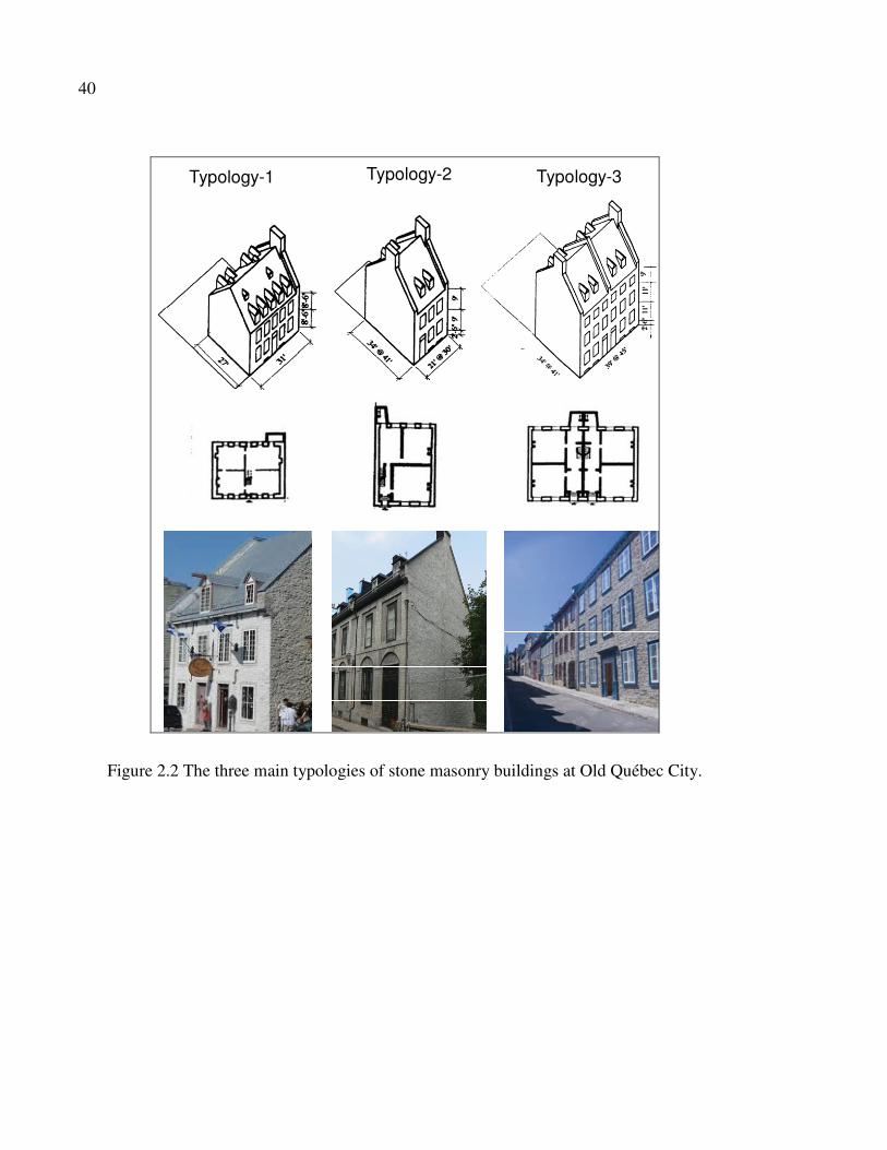
40
Typology-1 Typology-2 Typology-3
Figure 2.2 The three main typologies of stone masonry buildings at Old Québec City.

41
2.4 Displacement based damage model
The relatively good statistical correlation observed between the earthquake induced
displacement and the extent of structural damage contributed to the development of modern
performance-based seismic assessment methods. These methods consist of the evaluation of
the structure-specific deformation capacity and earthquake-induced displacement demand
(Ruiz-García and Negrete, 2009).
Building structural seismic performance is assessed using mechanical quantities, such as
inter-story drift, related to the physical condition of the building following an earthquake. For
evaluation of the structural performance, it is of interest that these mechanical quantities do
not exceed given threshold values defined as damage states (e.g. slight, moderate, extensive
and complete). These damage states represent the undesirable condition that has direct
consequence on building use during and after an earthquake and on the expected economic
and social losses. Well-defined and realistic damage states are extremely important due to
their direct impact on the fragility function parameters.
Simplified displacement-based procedures were proposed for assessment of the structural
performance of masonry structures (Calvi, 1999; Restrepo-Vélez, 2003). In these procedures,
damage of masonry structures is related to the capacity of in-plane loaded walls to sustain the
top of the wall horizontal displacement (drift). Note that masonry walls can be subjected to
out-of-plane failure mode orthogonal to the earthquake direction, depending mainly on the
quality of floor to wall connection. In this case, walls can fail locally especially at top stories
where dynamic amplification is higher. However, for walls that are properly anchored to
floors, the out-of-plane behavior should not be critical and the building damage is governed
by the in-plane behavior. This assumption is valid for most of the existing stone masonry
buildings in the Old Québec City, which were provided with steel anchors for improvements
in the floor to wall connections.
The procedure for assessment of the structural performance proposed by Restrepo-Vélez
(2003) is adopted in this study. For the MDOF masonry structure, a linear shape is assumed
for the elastic behavior, whereas a soft first story deformed shape is assumed for the inelastic

42
behavior (Figure 2.3a). The later is the most common failure mechanism of masonry
structures under earthquake loading (Tomaževic, 1999). The procedure assumes modeling of
the masonry structure as an ESDOF with effective global parameters. The displacement
threshold relative to a given structural damage state at the effective height of the ESDOF,
equivalent to the spectral displacement ( ,d DSiS ) in Equation 2.2, is obtained based on the
assumed deformed shape of the structure.
Drift thresholds for masonry walls are generally identified from laboratory experiments on
masonry wall elements. Drift threshold on the ESDOF of each damage state, ,d DSiS , is defined
as follows:
, 1 1 1 2( )d DSi DS DSi DS sS k H k hθ θ θ= + − (2.2)
where, H is total height of the building, sh is height of the first story, 1DSθ is drift threshold
for the first story walls at the elastic limit, DSiθ is the drift threshold for the first story walls at
higher damage states in the non-linear domain, 1k is the effective height coefficient of the
building at which the displacement of the MDOF system equals the spectral displacement for
an ESDOF system, and 2k is the effective height of the first story walls with openings that
deform in the inelastic range. The respective values for the studied two story buildings are k1
= 0.7 and k2 = 0.95 (Restrepo-Vélez 2003).
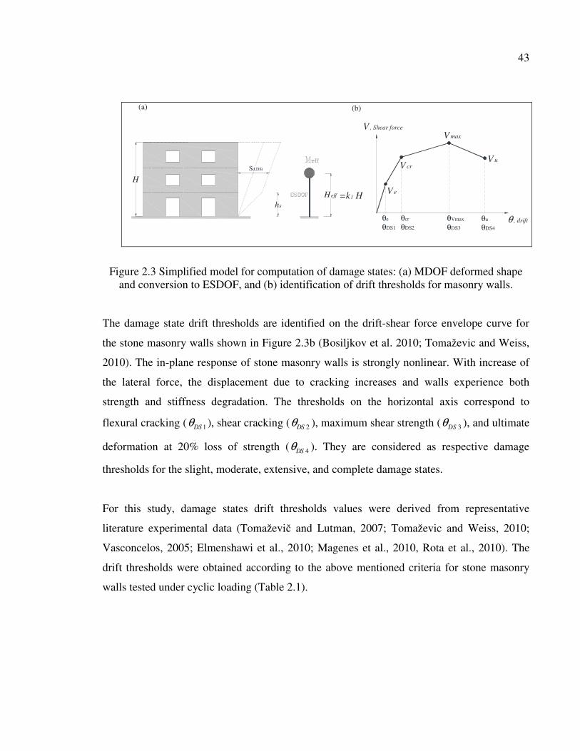
43
θe
θDS1
θcr
θDS2
θVmax
θDS3
θu
θDS4
Heff
hs
H
(a) (b)
θ , drift
V , Shear force
V e
V cr
V max
V uSd,DSi
.
=k1 H
Figure 2.3 Simplified model for computation of damage states: (a) MDOF deformed shape and conversion to ESDOF, and (b) identification of drift thresholds for masonry walls.
The damage state drift thresholds are identified on the drift-shear force envelope curve for
the stone masonry walls shown in Figure 2.3b (Bosiljkov et al. 2010; Tomaževic and Weiss,
2010). The in-plane response of stone masonry walls is strongly nonlinear. With increase of
the lateral force, the displacement due to cracking increases and walls experience both
strength and stiffness degradation. The thresholds on the horizontal axis correspond to
flexural cracking ( 1DSθ ), shear cracking ( 2DSθ ), maximum shear strength ( 3DSθ ), and ultimate
deformation at 20% loss of strength ( 4DSθ ). They are considered as respective damage
thresholds for the slight, moderate, extensive, and complete damage states.
For this study, damage states drift thresholds values were derived from representative
literature experimental data (Tomaževi� and Lutman, 2007; Tomaževic and Weiss, 2010;
Vasconcelos, 2005; Elmenshawi et al., 2010; Magenes et al., 2010, Rota et al., 2010). The
drift thresholds were obtained according to the above mentioned criteria for stone masonry
walls tested under cyclic loading (Table 2.1).

44
Table 2.1 Drift ratios for damage state thresholds for stone masonry walls.
Sample number �DS1 [%] �DS2 [%] �DS3 [%] �DS4 [%] 1 0.06 0.10 0.28 0.45 2 0.07 0.13 0.34 0.46 3 0.07 0.20 0.36 0.48 4 0.08 0.20 0.40 0.51 5 0.08 0.26 0.41 0.61 6 0.08 0.28 0.41 0.67 7 0.09 0.30 0.58 0.86 8 0.09 0.30 0.60 1.00 9 0.09 0.30 0.70 1.00
10 0.10 0.41 0.80 1.20 11 0.10 0.41 1.15 1.83 12 0.10 0.47 1.19 1.92 13 0.11 0.50 1.19 2.01 14 0.12 0.57 1.38 2.14 15 0.12 0.66 1.42 2.33 16 0.13 0.85 1.65 2.33
The empirical cumulative distribution function (CDF) for each damage state was obtained by
sorting the drift data in ascending order, and plotting them against a probability equal to
i/(n+1), where i is position of the drift ratio and n is the size of the sample (Ruiz-García and
Negrete, 2009). A lognormal CDF was then fitted with the advantage of being fully defined
by only two statistical parameters: the central tendency (median) and dispersion (lognormal
standard deviation) (Figure 2.4). These values were then implemented in Equation 2.2 to
simulate the displacement of the ESDOF system. The story height was assumed to have a
fixed value equal to the median height observed from the inventory ( sh =3.0 m). The resulting
displacement threshold data were then represented with lognormal distributions which
actually represent the displacement fragility functions for the ESDOF system (Table 2.2).

45
0 0.5 1 1.5 2 2.50
0.2
0.4
0.6
0.8
1
Drift Ratio [%]
P(D
Si |
drif
t rat
io)
DS1 (Slight)DS2 (Moderate)DS3 (Extensive)DS4 (Complete)data5data6data7data8
Lognormal CDF
Empirical CDF
Figure 2.4: Drift threshold variability for low-rise stone masonry buildings.
Table 2.2 Median and dispersion of the displacement based damage states for two story stone masonry building and respective values implicit in Hazus and ELER
Quebec Stone
low-rise (two-story)
ELER stone
low-rise
Hazus pre-code
URM low-rise
Damage state Median
Sd [m]
Dispersion
�T
Median
Sd [m]
Dispersion
�T
Median
Sd [m]
Dispersion
�T
DS1 [Slight] 0.005 0.20 0.002 0.4 0.008 0.4
DS2 [Moderate] 0.012 0.38 0.004 0.4 0.016 0.4
DS3 [Extensive] 0.021 0.40 0.007 0.4 0.041 0.4
DS4 [Complete] 0.028 0.50 0.011 0.4 0.096 0.4
Figure 2.5 illustrates the developed fragility functions for the considered low-rise stone
masonry building compared to respective fragility functions implicit in Hazus (pre-code low-
rise unreinforced masonry buildings) and ELER (simple stone low-rise buildings). The
difference in the respective fragility functions comes from the information used in their
developments. For Hazus and ELER, the median and standard deviation for different damage
46
states are based on empirical data and expert opinion. The respective dispersion is assumed
constant for all damage states, , 0.4T DSiβ = . On the other hand, the developed fragility curves
in this study are based on observed experimental behaviour of stone walls where dispersion
comes from the variability of specimen-to-specimen testing data. The dispersion is the lowest
for slight damage state, , 1 0.2T DSβ = , and is highest for complete damage state, , 4 0.5T DSβ = .
This increase in dispersion results from the rapid degradation of stone walls with increasing
displacement demand and imprecisions in recording the respective displacement accurately.
Moreover, the large variety in specimen-to-specimen mechanical properties and stone block
arrangement of the tested walls contribute to increasing the dispersion in the identification of
higher damage state thresholds.
Limitations exist regarding the direct comparison of fragility functions between different
models because of the different assumptions, information and tools used in the development
process. Hence, the objective of the comparison given in Figure 2.5 is rather to show the
importance for the development of fragility functions that reflect the specific characteristics
of the considered structures.
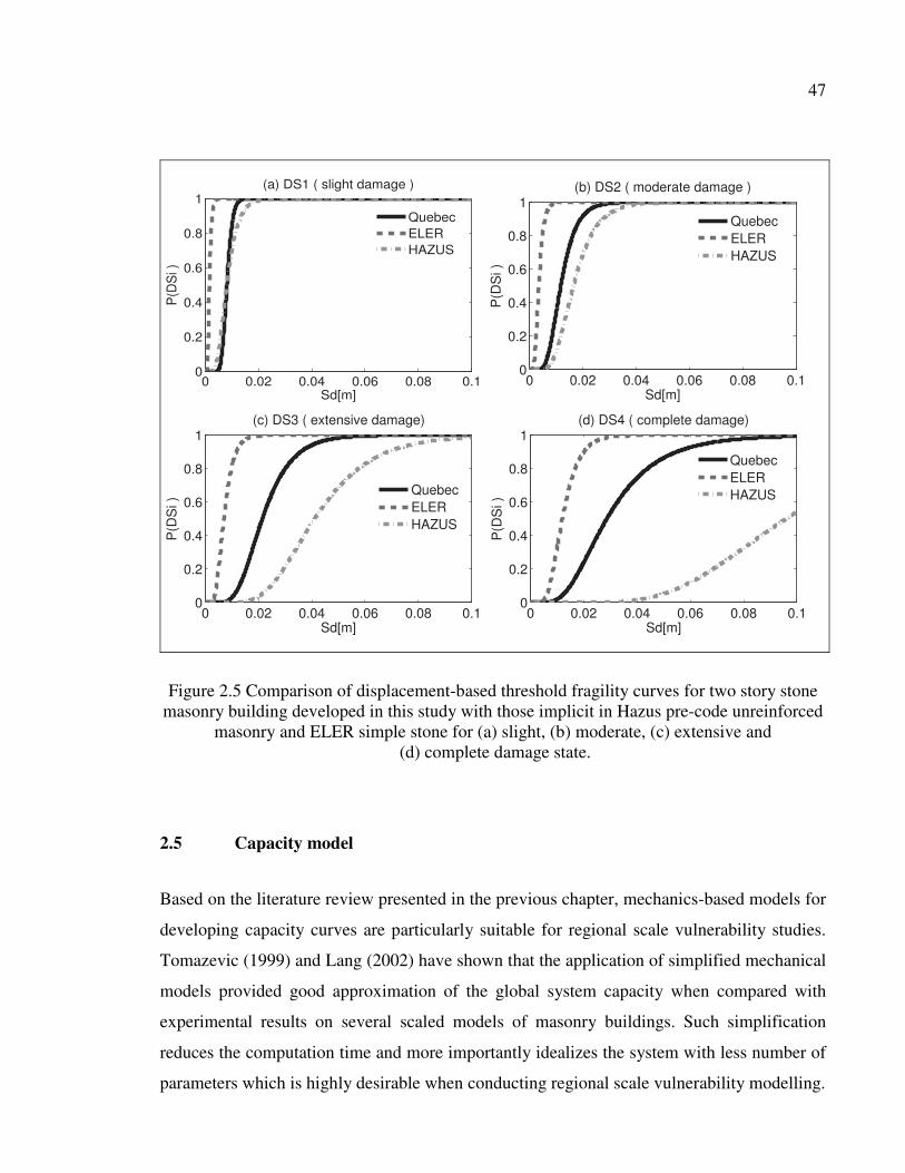
47
0 0.02 0.04 0.06 0.08 0.10
0.2
0.4
0.6
0.8
1
Sd[m]
P(D
Si )
(d) DS4 ( complete damage)
QuebecELERHAZUS
0 0.02 0.04 0.06 0.08 0.10
0.2
0.4
0.6
0.8
1
Sd[m]
P(D
Si )
(a) DS1 ( slight damage )
QuebecELERHAZUS
0 0.02 0.04 0.06 0.08 0.10
0.2
0.4
0.6
0.8
1
Sd[m]
P(D
Si )
(b) DS2 ( moderate damage )
QuebecELERHAZUS
0 0.02 0.04 0.06 0.08 0.10
0.2
0.4
0.6
0.8
1
Sd[m]
P(D
Si )
(c) DS3 ( extensive damage)
QuebecELERHAZUS
Figure 2.5 Comparison of displacement-based threshold fragility curves for two story stone masonry building developed in this study with those implicit in Hazus pre-code unreinforced
masonry and ELER simple stone for (a) slight, (b) moderate, (c) extensive and (d) complete damage state.
2.5 Capacity model
Based on the literature review presented in the previous chapter, mechanics-based models for
developing capacity curves are particularly suitable for regional scale vulnerability studies.
Tomazevic (1999) and Lang (2002) have shown that the application of simplified mechanical
models provided good approximation of the global system capacity when compared with
experimental results on several scaled models of masonry buildings. Such simplification
reduces the computation time and more importantly idealizes the system with less number of
parameters which is highly desirable when conducting regional scale vulnerability modelling.
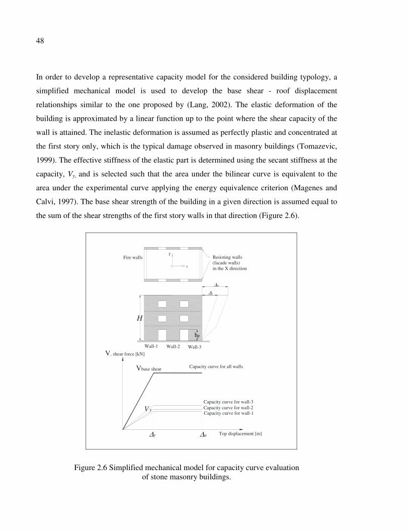
48
In order to develop a representative capacity model for the considered building typology, a
simplified mechanical model is used to develop the base shear - roof displacement
relationships similar to the one proposed by (Lang, 2002). The elastic deformation of the
building is approximated by a linear function up to the point where the shear capacity of the
wall is attained. The inelastic deformation is assumed as perfectly plastic and concentrated at
the first story only, which is the typical damage observed in masonry buildings (Tomazevic,
1999). The effective stiffness of the elastic part is determined using the secant stiffness at the
capacity, Vy, and is selected such that the area under the bilinear curve is equivalent to the
area under the experimental curve applying the energy equivalence criterion (Magenes and
Calvi, 1997). The base shear strength of the building in a given direction is assumed equal to
the sum of the shear strengths of the first story walls in that direction (Figure 2.6).
x
YResisting walls(facade walls)in the X direction
Top displacement [m]
V, shear force [kN]
Capacity curve for all walls
V y
ΔuΔy
Vbase shear
Δy
H
Fire walls
Δu.
.
hp
Wall-1 Wall-2 Wall-3
Capacity curve for wall-1Capacity curve for wall-2Capacity curve for wall-3
Figure 2.6 Simplified mechanical model for capacity curve evaluation of stone masonry buildings.
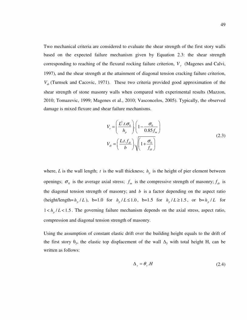
49
Two mechanical criteria are considered to evaluate the shear strength of the first story walls
based on the expected failure mechanism given by Equation 2.3: the shear strength
corresponding to reaching of the flexural rocking failure criterion, rV (Magenes and Calvi,
1997), and the shear strength at the attainment of diagonal tension cracking failure criterion,
dtV (Turnsek and Cacovic, 1971). These two criteria provided good approximation of the
shear strength of stone masonry walls when compared with experimental results (Mazzon,
2010; Tomazevic, 1999; Magenes et al., 2010; Vasconcelos, 2005). Typically, the observed
damage is mixed flexure and shear failure mechanisms.
20 0
0
. .. 1
0.85
. .. 1
rp m
dtdt
dt
L tV
h f
L t fV
b f
σ σ
σ
� � � �= − � �� �
� �� �= + � � � �
(2.3)
where, L is the wall length; t is the wall thickness; ph is the height of pier element between
openings; 0σ is the average axial stress; mf is the compressive strength of masonry; dtf is
the diagonal tension strength of masonry; and b is a factor depending on the aspect ratio
(height/length= /ph L ), b=1.0 for / 1.0ph L ≤ , b=1.5 for / 1.5ph L ≥ , or b= /ph L for
1 / 1.5ph L< < . The governing failure mechanism depends on the axial stress, aspect ratio,
compression and diagonal tension strength of masonry.
Using the assumption of constant elastic drift over the building height equals to the drift of
the first story �y, the elastic top displacement of the wall �y with total height H, can be
written as follows:
.y y HθΔ = (2.4)
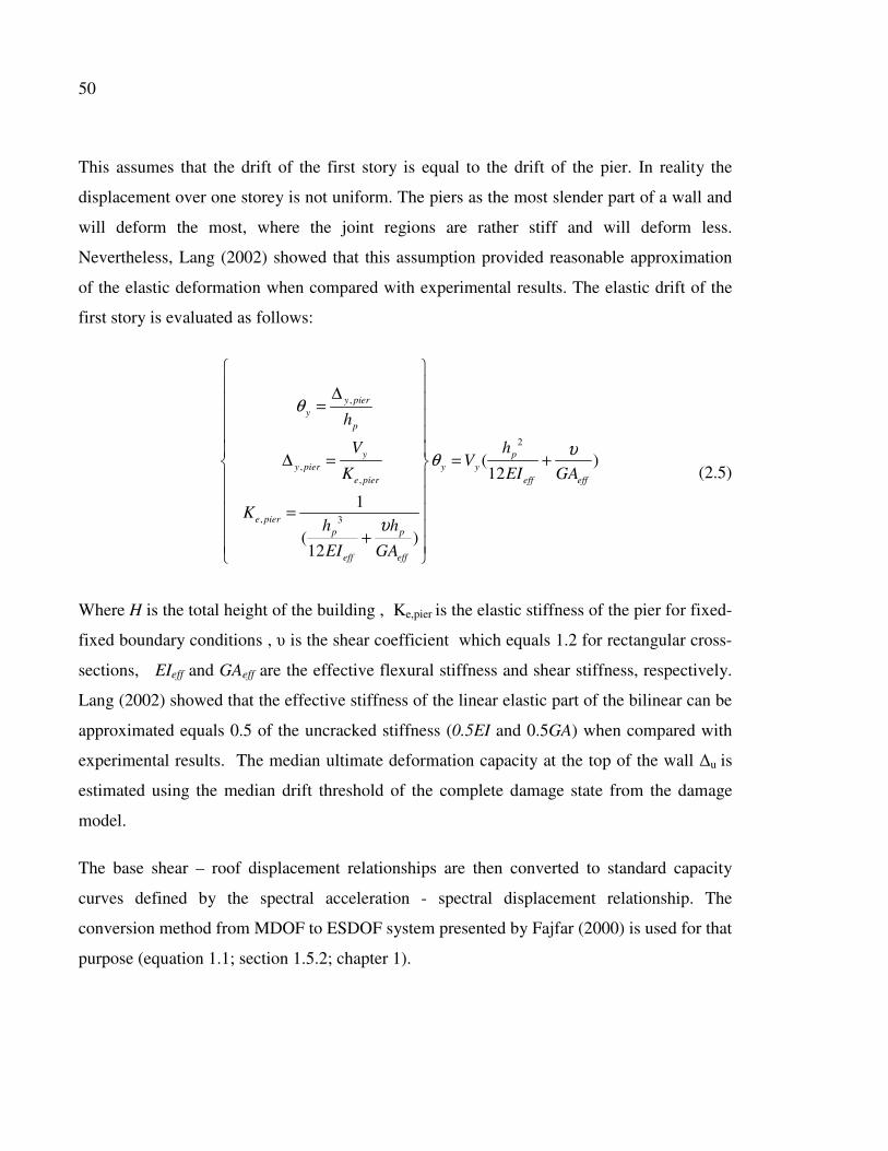
50
This assumes that the drift of the first story is equal to the drift of the pier. In reality the
displacement over one storey is not uniform. The piers as the most slender part of a wall and
will deform the most, where the joint regions are rather stiff and will deform less.
Nevertheless, Lang (2002) showed that this assumption provided reasonable approximation
of the elastic deformation when compared with experimental results. The elastic drift of the
first story is evaluated as follows:
,
2
,,
, 3
( )12
1
( )12
y piery
p
y py pier y y
e pier eff eff
e pierp p
eff eff
h
V hV
K EI GA
Kh h
EI GA
θ
υθ
υ
� �� �� �=� �� �� �
Δ = = +� �� �� �
=� �� �+� �� �
(2.5)
Where H is the total height of the building , Ke,pier is the elastic stiffness of the pier for fixed-
fixed boundary conditions , is the shear coefficient which equals 1.2 for rectangular cross-
sections, EIeff and GAeff are the effective flexural stiffness and shear stiffness, respectively.
Lang (2002) showed that the effective stiffness of the linear elastic part of the bilinear can be
approximated equals 0.5 of the uncracked stiffness (0.5EI and 0.5GA) when compared with
experimental results. The median ultimate deformation capacity at the top of the wall �u is
estimated using the median drift threshold of the complete damage state from the damage
model.
The base shear – roof displacement relationships are then converted to standard capacity
curves defined by the spectral acceleration - spectral displacement relationship. The
conversion method from MDOF to ESDOF system presented by Fajfar (2000) is used for that
purpose (equation 1.1; section 1.5.2; chapter 1).
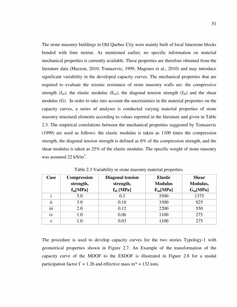
51
The stone masonry buildings in Old Quebec City were mainly built of local limestone blocks
bonded with lime mortar. As mentioned earlier, no specific information on material
mechanical properties is currently available. These properties are therefore obtained from the
literature data (Mazzon, 2010; Tomazevic, 1999, Magenes et al., 2010) and may introduce
significant variability in the developed capacity curves. The mechanical properties that are
required to evaluate the seismic resistance of stone masonry walls are: the compressive
strength (fm), the elastic modulus (Em), the diagonal tension strength (fdt) and the shear
modulus (G). In order to take into account the uncertainties in the material properties on the
capacity curves, a series of analyses is conducted varying material properties of stone
masonry structural elements according to values reported in the literature and given in Table
2.3. The empirical correlations between the mechanical properties suggested by Tomazevic
(1999) are used as follows: the elastic modulus is taken as 1100 times the compression
strength, the diagonal tension strength is defined as 6% of the compression strength, and the
shear modulus is taken as 25% of the elastic modulus. The specific weight of stone masonry
was assumed 22 kN/m3.
Table 2.3 Variability in stone masonry material properties.
Case Compression strength, fm[MPa]
Diagonal tension strength, fdt [MPa]
Elastic Modulus Em[MPa]
Shear Modulus, Gm[MPa]
i 5.0 0.3 5500 1375 ii 3.0 0.18 3300 825 iii 2.0 0.12 2200 550 iv 1.0 0.06 1100 275 v 1.0 0.03 1100 275
The procedure is used to develop capacity curves for the two stories Typology-1 with
geometrical properties shown in Figure 2.7. An Example of the transformation of the
capacity curve of the MDOF to the ESDOF is illustrated in Figure 2.8 for a modal
participation factor � = 1.26 and effective mass m* = 132 tons.
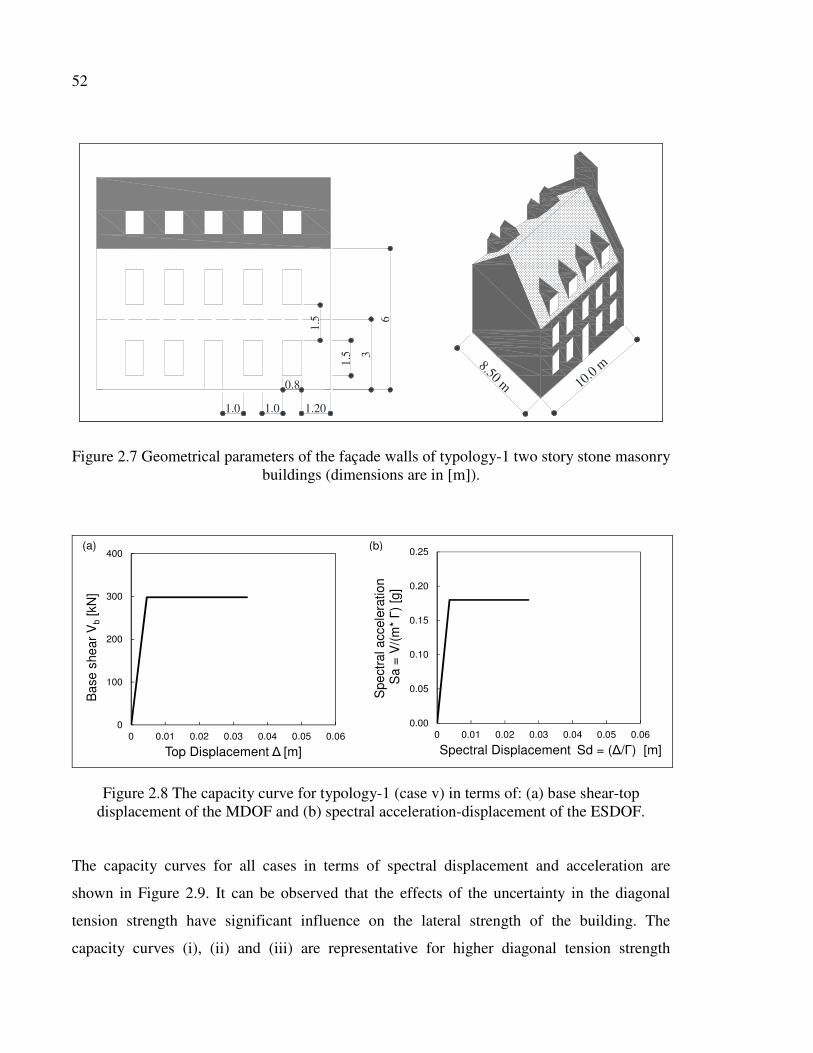
52
1.5 3
6
1.5
0.8
1.01.0 1.20
10.0
m8.50 m
Figure 2.7 Geometrical parameters of the façade walls of typology-1 two story stone masonry buildings (dimensions are in [m]).
0
100
200
300
400
0 0.01 0.02 0.03 0.04 0.05 0.06
Bas
e sh
ear
Vb
[kN
]
Top Displacement � [m]
0.00
0.05
0.10
0.15
0.20
0.25
0 0.01 0.02 0.03 0.04 0.05 0.06
Spe
ctra
l acc
eler
atio
nS
a =
V/(
m* �)
[g]
Spectral Displacement Sd = (�/�) [m]
(a) (b)
Figure 2.8 The capacity curve for typology-1 (case v) in terms of: (a) base shear-top displacement of the MDOF and (b) spectral acceleration-displacement of the ESDOF.
The capacity curves for all cases in terms of spectral displacement and acceleration are
shown in Figure 2.9. It can be observed that the effects of the uncertainty in the diagonal
tension strength have significant influence on the lateral strength of the building. The
capacity curves (i), (ii) and (iii) are representative for higher diagonal tension strength
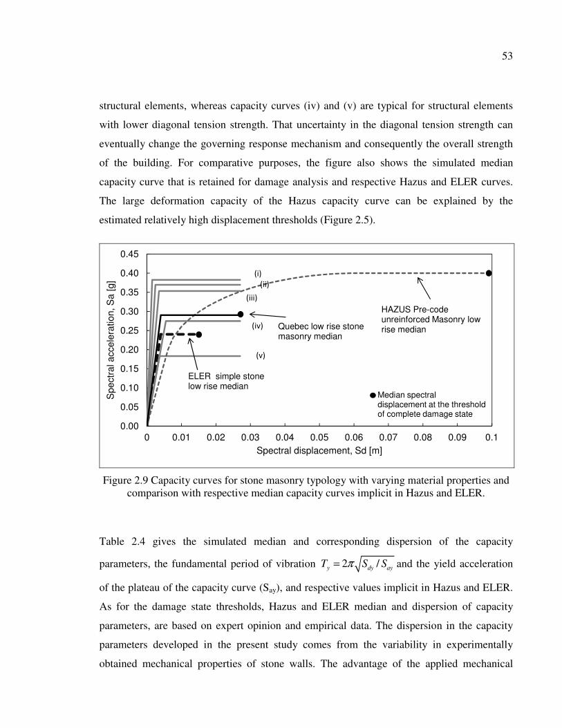
53
structural elements, whereas capacity curves (iv) and (v) are typical for structural elements
with lower diagonal tension strength. That uncertainty in the diagonal tension strength can
eventually change the governing response mechanism and consequently the overall strength
of the building. For comparative purposes, the figure also shows the simulated median
capacity curve that is retained for damage analysis and respective Hazus and ELER curves.
The large deformation capacity of the Hazus capacity curve can be explained by the
estimated relatively high displacement thresholds (Figure 2.5).
0.00
0.05
0.10
0.15
0.20
0.25
0.30
0.35
0.40
0.45
0 0.01 0.02 0.03 0.04 0.05 0.06 0.07 0.08 0.09 0.1
Spe
ctra
l acc
eler
atio
n, S
a [g
]
Spectral displacement, Sd [m]
ELER simple stonelow rise median
HAZUS Pre-codeunreinforced Masonry low rise median
����
��
��
��
Median spectral displacement at the threshold of complete damage state
Quebec low rise stone masonry median
Figure 2.9 Capacity curves for stone masonry typology with varying material properties and comparison with respective median capacity curves implicit in Hazus and ELER.
Table 2.4 gives the simulated median and corresponding dispersion of the capacity
parameters, the fundamental period of vibration 2 /y dy ayT S Sπ= and the yield acceleration
of the plateau of the capacity curve (Say), and respective values implicit in Hazus and ELER.
As for the damage state thresholds, Hazus and ELER median and dispersion of capacity
parameters, are based on expert opinion and empirical data. The dispersion in the capacity
parameters developed in the present study comes from the variability in experimentally
obtained mechanical properties of stone walls. The advantage of the applied mechanical

54
model is the flexibility for investigation and quantification of uncertainties. The applied
mechanical model can also be applied to explore the potential effects of retrofitting on the
increase of the seismic capacity of the building in a simplified manner. Analyses were also
conducted to develop the capacity parameters for one and three stories stone masonry
building typologies (Appendix-I).
Table 2.4 Median and dispersion of capacity parameters of stone masonry buildings and respective values implicit in Hazus and ELER
Quebec
stone,
low-rise
ELER stone,
low-rise
Hazus pre-
code URM ,
low-rise
Median fundamental period of vibration
Ty [sec]
0.18 0.19 0.35
Dispersion fundamental period of
vibration (�) Ty [sec]
0.34 - -
Median yield acceleration Say [g] 0.30 0.24 0.20
Dispersion yield acceleration (�) Say [g] 0.26 0.30 0.30
2.6 Seismic demand model
In this section, the contribution of the variability in the seismic demand on the fragility of
stone masonry buildings is discussed. The seismic behavior of structures is characterized by
the amount of damage, indicating that inelastic deformation occurred during the earthquake.
As the linear analysis cannot predict such behavior in an explicit manner, nonlinear analysis
is generally applied using nonlinear static or dynamic time history analyses. While the later is
time consuming and requires detailed selection and scaling of the ground motion records
prior to conducting the dynamic response analysis, the nonlinear static analysis represents a
simple and reasonably accurate alternative. It is particularly effective for low-rise buildings
dominated by the first mode response (FEMA, 2005). Ruiz-Garcia and Miranda (2007)
proposed an attractive nonlinear static procedure which includes the uncertainty in the
seismic demand. It applies statistical analysis of the displacement demand predicted from the

55
dynamic response of nonlinear SDOF systems subjected to a series of ground motions to
obtain a simplified expression for median and dispersion of displacement demand. The
procedure used for assessing the combined variability in capacity and seismic demand,
( , )C DCONV β β in Equation 2.1 consists of the following steps:
1) The capacity parameters, median and standard deviation values of the fundamental period
and yield acceleration (Ty, Say), are obtained based on the probability distribution
presented in (Table 2.4).
2) The spectral displacement response (Sd) is evaluated for each sampled pair of capacity
parameters at different levels of seismic demand using the displacement coefficient
method (FEMA, 2005). This widely used nonlinear static procedure essentially modifies
the elastic response of the ESDOF system with 5% damping by multiplication with a
series of coefficients to generate an estimate of the inelastic displacement demand, dS , as
follows,
( )
2
1 2 2
1 2
2
2
. . ( ). .4.
11
.
1 11
800
yd a y
y
y
a y
ay
TS C C S T g
RC
a T
RC
T
S TR
S
π=
−= +
� �−= + � �
� � �
=
(2.6)
where, 1C is modification parameter which relates the expected maximum displacement
of an inelastic ESDOF system with elastic-plastic hysteresis properties to the
displacement calculated from the elastic spectral response; 2C accounts for the effects of
pinched hysteresis shape, stiffness degradation, and strength deterioration on the
maximum displacement response; ( )a yS T
is the spectral acceleration at the fundamental
period of the system, Ty; a is a constant referring to the site class (a=130 for site class B,
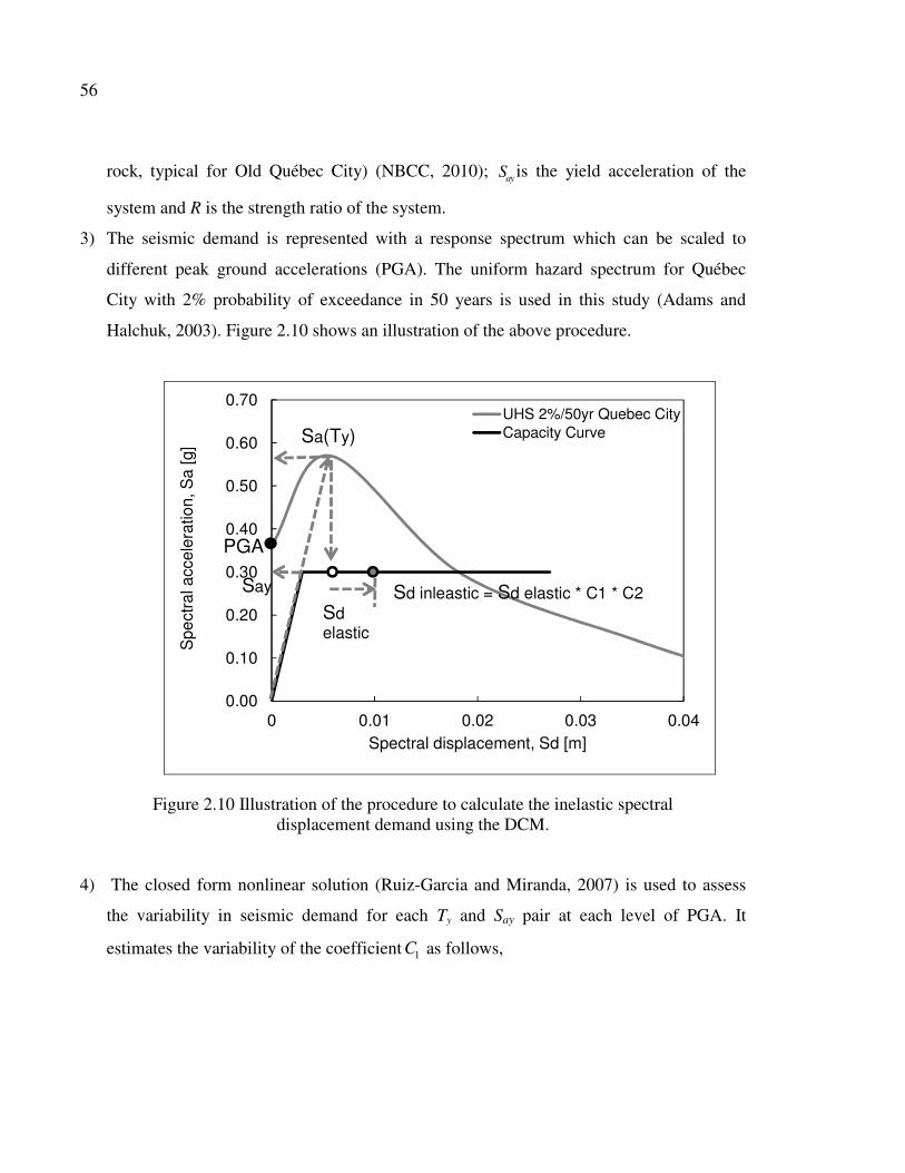
56
rock, typical for Old Québec City) (NBCC, 2010); ayS is the yield acceleration of the
system and R is the strength ratio of the system.
3) The seismic demand is represented with a response spectrum which can be scaled to
different peak ground accelerations (PGA). The uniform hazard spectrum for Québec
City with 2% probability of exceedance in 50 years is used in this study (Adams and
Halchuk, 2003). Figure 2.10 shows an illustration of the above procedure.
0.00
0.10
0.20
0.30
0.40
0.50
0.60
0.70
0 0.01 0.02 0.03 0.04
Spe
ctra
l acc
eler
atio
n, S
a [g
]
Spectral displacement, Sd [m]
UHS 2%/50yr Quebec CityCapacity CurveSa(Ty)
Say
R
PGA
Sd inleastic = Sd elastic * C1 * C2Sd elastic
Figure 2.10 Illustration of the procedure to calculate the inelastic spectral displacement demand using the DCM.
4) The closed form nonlinear solution (Ruiz-Garcia and Miranda, 2007) is used to assess
the variability in seismic demand for each Ty and Say pair at each level of PGA. It
estimates the variability of the coefficient 1C as follows,

57
[ ]
1
1 2
3 4
1 1.
.( 0.1)
. 1 exp( ( 1))
C A A T
A A R
β α
α
� �= +� �+ �
= − − −
(2.7)
where, A1 = 5.876, A2 = 11.749, A3 = 1.957, and A4 = 0.739. The above procedure allows
obtaining the lognormal distribution parameters for the inelastic displacement demand,
i.e., lognormal median ( ) ln( )Sd j dPGA Sλ = from Equation 2.6 and lognormal standard
deviation ( )Sd jPGAβ from Equation 2.7. Figure 2.11 shows an illustration of the
probability distribution of the inelastic displacement demand at a given PGA. Table 2.5
shows example calculations for the displacement demand.
0.00
0.40
0.80
1.20
0 0.01 0.02 0.03 0.04
Spe
ctra
l acc
eler
atio
n, S
a [g
]
Spectral displacement, Sd [m]
Capacity Curve
UHS 2%/50yr Quebec City
Scaled Spectrum
PGAj
( ) ( )
displacement demand
( , ) Sd PGAj Sd PGAjλ β
Figure 2.11 Illustration of the variability in displacement demand at a given level of PGA.
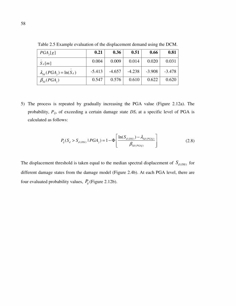
58
Table 2.5 Example evaluation of the displacement demand using the DCM.
[ ]jPGA g 0.21 0.36 0.51 0.66 0.81
[ ]dS m−
0.004 0.009 0.014 0.020 0.031
( ) ln( )dSd jPGA Sλ−
= -5.413 -4.657 -4.238 -3.908 -3.478
( )Sd jPGAβ 0.547 0.576 0.610 0.622 0.620
5) The process is repeated by gradually increasing the PGA value (Figure 2.12a). The
probability, Pij, of exceeding a certain damage state DSi at a specific level of PGA is
calculated as follows:
( ) ( )
( )( )
ln( )( | ) 1 d DSi Sd PGAj
ij d d DSi jSd PGAj
SP S S PGA
λ
β
� �−> = − Φ � �
� � � (2.8)
The displacement threshold is taken equal to the median spectral displacement of ( )d DSiS for
different damage states from the damage model (Figure 2.4b). At each PGA level, there are
four evaluated probability values, ijP (Figure 2.12b).
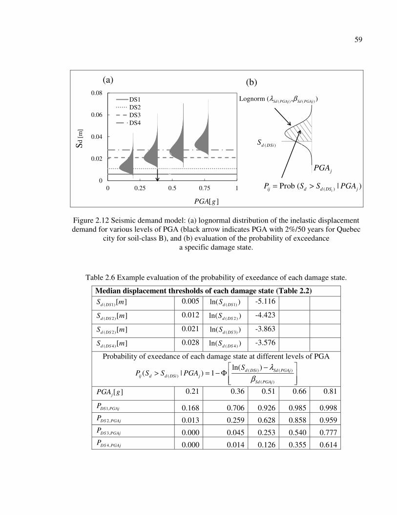
59
�
��� ���
��� ���
��� ���
��� ���
���
� ��
����
���
��
��
( )Prob ( | )iij d d DS jP S S PGA= >
jPGA
( ) ( )Lognorm ( , ) Sd PGAj Sd PGAjλ β
Sd[m
]
[ ]PGA g
0
0.02
0.04
0.06
0.08
0 0.25 0.5 0.75 1
DS1DS2DS3DS4
( )
( )d DSiS
(a) (b)
Figure 2.12 Seismic demand model: (a) lognormal distribution of the inelastic displacement demand for various levels of PGA (black arrow indicates PGA with 2%/50 years for Quebec
city for soil-class B), and (b) evaluation of the probability of exceedance a specific damage state.
Table 2.6 Example evaluation of the probability of exeedance of each damage state.
Median displacement thresholds of each damage state (Table 2.2)
( 1)[ ]d DSS m 0.005 ( 1)ln( )d DSS -5.116
( 2)[ ]d DSS m 0.012 ( 2)ln( )d DSS -4.423
( 2)[ ]d DSS m 0.021 ( 3)ln( )d DSS -3.863
( 4)[ ]d DSS m 0.028 ( 4)ln( )d DSS -3.576
Probability of exeedance of each damage state at different levels of PGA
( ) ( )( )
( )
ln( )( | ) 1 d DSi Sd PGAj
ij d d DSi jSd PGAj
SP S S PGA
λ
β
� �−> = − Φ � �
� � �
[ ]jPGA g 0.21 0.36 0.51 0.66 0.81
1,DS PGAjP 0.168 0.706 0.926 0.985 0.998
2,DS PGAjP 0.013 0.259 0.628 0.858 0.959
3,DS PGAjP 0.000 0.045 0.253 0.540 0.777
4,DS PGAjP 0.000 0.014 0.126 0.355 0.614
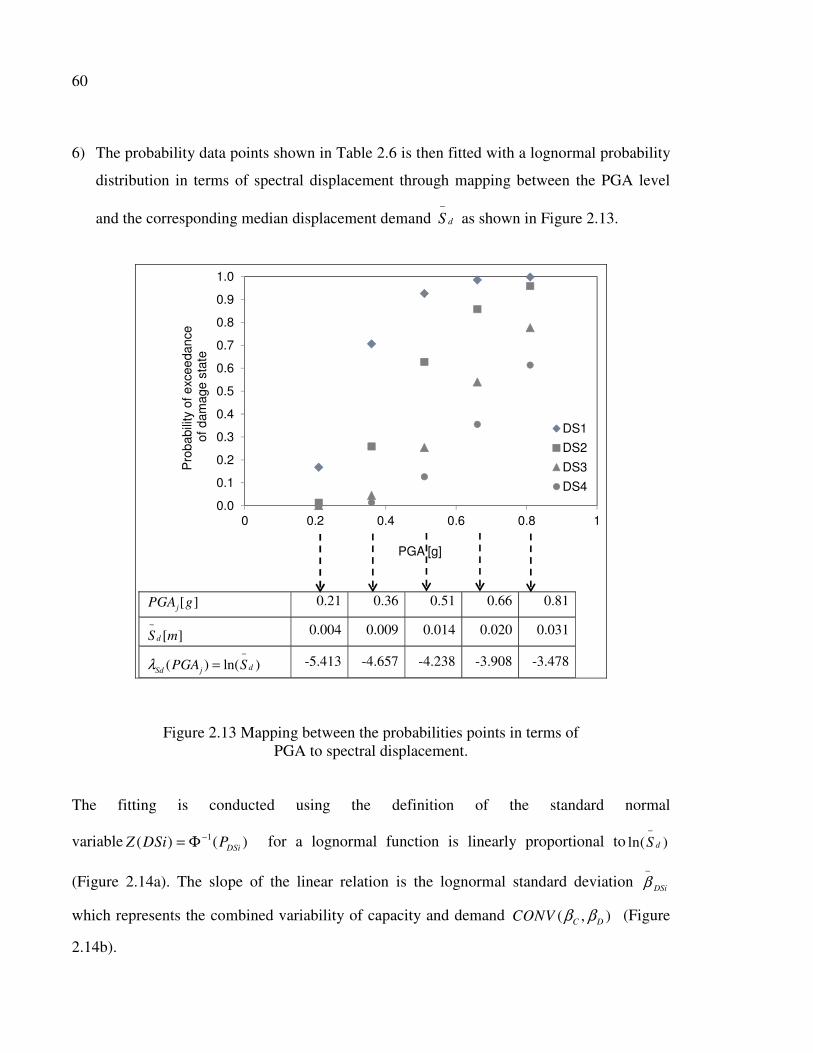
60
6) The probability data points shown in Table 2.6 is then fitted with a lognormal probability
distribution in terms of spectral displacement through mapping between the PGA level
and the corresponding median displacement demand dS−
as shown in Figure 2.13.
[ ]jPGA g 0.21 0.36 0.51 0.66 0.81
[ ]dS m−
0.004 0.009 0.014 0.020 0.031
( ) ln( )dSd jPGA Sλ−
= -5.413 -4.657 -4.238 -3.908 -3.478
0.0
0.1
0.2
0.3
0.4
0.5
0.6
0.7
0.8
0.9
1.0
0 0.2 0.4 0.6 0.8 1
Pro
babi
lity
of e
xcee
danc
eof
dam
age
stat
e
PGA [g]
DS1
DS2
DS3
DS4
Figure 2.13 Mapping between the probabilities points in terms of PGA to spectral displacement.
The fitting is conducted using the definition of the standard normal
variable 1( ) ( )DSiZ DSi P−= Φ for a lognormal function is linearly proportional to ln( )dS−
(Figure 2.14a). The slope of the linear relation is the lognormal standard deviation DSiβ−
which represents the combined variability of capacity and demand ( , )C DCONV β β (Figure
2.14b).

61
0.0
0.1
0.2
0.3
0.4
0.5
0.6
0.7
0.8
0.9
1.0
0.000 0.010 0.020 0.030 0.040
Prob
abil
ity o
f ex
ceed
ance
of d
amag
e st
ate
Sd [m]
DS1
DS2
DS3
DS4
(b)
-6
-5
-4
-3-5 -3 -1 1 3 5
Standard normal variable (Z)
DS1DS2DS3DS4
(a)
ln( )dS−
(a)
(b)
( , )DSi c DCONVβ β β−
=
Figure 2.14 Fitting of the probability distribution of combined uncertainty of capacity and demand parameters for different damage state (a) the standard normal variable domain and
(b) the cumulative lognormal functions.
The final displacement based fragility function lognormal distributed are given in (Table 2.7)
along with the respective values implicit in Hazus and ELER. The DSiβ−
=
( , )C DCONV β β value combined with the lognormal standard deviations of the damage state
thresholds, Tβ , obtained from the damage model (Table 2.2) yields the total lognormal
standard deviation for each damage state 2 2( , )DS C D TCONVβ β β β= + ).
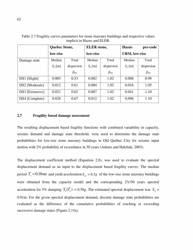
62
Table 2.7 Fragility curves parameters for stone masonry buildings and respective values implicit in Hazus and ELER.
Quebec Stone,
low-rise
ELER stone,
low-rise
Hazus pre-code
URM, low-rise
Damage state Median
Sd [m]
Total
dispersion
�DS
Median
Sd [m]
Total
dispersion
�DS
Median
Sd [m]
Total
dispersion
�DS
DS1 [Slight] 0.005 0.53 0.002 1.02 0.008 0.99
DS2 [Moderate] 0.012 0.61 0.004 1.02 0.016 1.05
DS3 [Extensive] 0.021 0.62 0.007 1.02 0.041 1.10
DS4 [Complete] 0.028 0.67 0.012 1.02 0.096 1.10
2.7 Fragility based damage assessment
The resulting displacement based fragility functions with combined variability in capacity,
seismic demand and damage state threshold, were used to determine the damage state
probabilities for low-rise stone masonry buildings in Old Québec City for seismic input
motion with 2% probability of exceedance in 50 years (Adams and Halchuk, 2003).
The displacement coefficient method (Equation 2.8), was used to evaluate the spectral
displacement demand as an input to the displacement based fragility curves. The median
period 0.18secyT = and yield acceleration 0.3ayS g= of the low-rise stone masonry buildings
were obtained from the capacity model and the corresponding 2%/50 years spectral
acceleration for 5% damping ( )a yS T = 0.58g. The estimated spectral displacement was dS =
0.01m. For the given spectral displacement demand, discrete damage state probabilities are
evaluated as the difference of the cumulative probabilities of reaching or exceeding
successive damage states (Figure 2.15a).
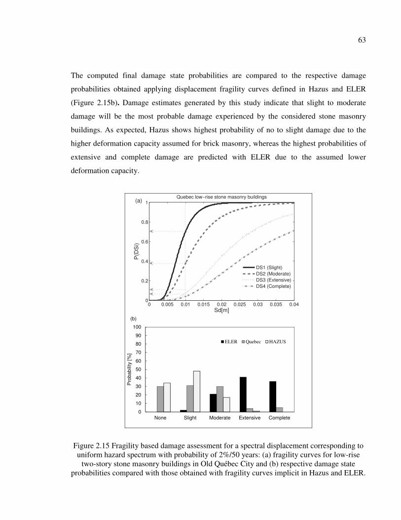
63
The computed final damage state probabilities are compared to the respective damage
probabilities obtained applying displacement fragility curves defined in Hazus and ELER
(Figure 2.15b). Damage estimates generated by this study indicate that slight to moderate
damage will be the most probable damage experienced by the considered stone masonry
buildings. As expected, Hazus shows highest probability of no to slight damage due to the
higher deformation capacity assumed for brick masonry, whereas the highest probabilities of
extensive and complete damage are predicted with ELER due to the assumed lower
deformation capacity.
0 0.005 0.01 0.015 0.02 0.025 0.03 0.035 0.040
0.2
0.4
0.6
0.8
1
Sd[m]
P(D
Si)
Quebec low−rise stone masonry buildings
DS1 (Slight)DS2 (Moderate)DS3 (Extensive)DS4 (Complete)
(a)
0
10
20
30
40
50
60
70
80
90
100
None Slight Moderate Extensive Complete
Pro
babi
lity
[%]
ELER Quebec HAZUS
(b)
Figure 2.15 Fragility based damage assessment for a spectral displacement corresponding to uniform hazard spectrum with probability of 2%/50 years: (a) fragility curves for low-rise
two-story stone masonry buildings in Old Québec City and (b) respective damage state probabilities compared with those obtained with fragility curves implicit in Hazus and ELER.
64
2.8 Summary and conclusions
A robust procedure for analytical displacement based fragility analysis of stone masonry
buildings was presented. Old Québec City was selected as a study area representative for
historical urban centers in Eastern Canada. The first step consisted of inventory of the
existing stone masonry buildings and characterization of representative typology. Respective
building capacity model was developed using a simplified mechanical model with linear
elastic and perfectly plastic domains. Displacement based procedure was then used to
develop damage state fragility functions, based on drift thresholds of stone masonry walls,
assigned based on literature data. A simplified probabilistic seismic demand analysis was
proposed to capture the combined uncertainty in capacity and demand on the fragility curves.
The generated fragility curves were determined for low-rise stone masonry buildings as
functions of spectral displacement. The results of damage assessment for a 2%/50 years
uniform hazard seismic scenario indicate that slight to moderate damage will be the most
probable damage experienced by these stone masonry buildings.
A comparison of the developed fragility functions was made with those implicit in the
seismic risk assessment tools Hazus and ELER. Significant differences have been observed.
These differences were replicated in comparatively significant disparities among the
probability estimates for different damages states. Hazus showed highest probability of
occurring no to slight damage due to the assumed higher deformation capacity, whereas the
highest probabilities of extensive and complete damage were predicted with ELER due to the
assumed lower deformation capacity. This comparative example showed the importance of
the development of specific fragility functions that reflect the generic construction
characteristics for the considered study area and emphasized the need of critical use of
existing risk assessment tools and the obtained results. It can be expected that using drift
thresholds and mechanical characterization obtained from laboratory testing of stone
masonry walls representative of those existing in Old Québec City would help to reduce the
uncertainties in the damage prediction.
65
The proposed methodology for fragility analysis can easily be applied to other building types
provided that damage state drift thresholds and material properties are available. It has
several advantages, first of all in the use of simplified mechanical models for capacity curves
generation which proved particularly effective for carrying out analyses of uncertainties with
significantly reduced computational time, and then in the use of experimental displacement
based damage criteria instead of relying on expert opinion. On the other hand, it does not
consider the possible out-of-plane failure mechanisms that might occur in case where poor
connection between floor and wall exists. This issue should be considered in future research.
In addition, the increased uncertainties in the identification of the complete damage state
from experimental data due to the rapid degradation of the stone walls after reaching peak
strength should also be taken into consideration.

CHAPTER 3
SEISMIC HAZARD COMPATIBLE VULNERABILITY MODELLING
3.1 Introduction
This chapter presents the results of an effective vulnerability analysis procedure for stone
masonry buildings in terms of seismic hazard compatible fragility and vulnerability functions
for sets of earthquake scenarios. This vulnerability analysis is based on the work developed
in the previous chapter work on stone masonry buildings that developed the two main inputs
for the vulnerability analysis: (1) capacity curves that characterize the nonlinear behaviour of
the existing stone masonry buildings and (2) displacement based fragility functions that
represent the probability of exceedance of specified damage state under various levels of
structural displacement response (e.g., slight, moderate, extensive, complete). These two
inputs are convolved with response spectra to estimate the structural damage to buildings for
a series of earthquake magnitude-distance combinations. The obtained results for typical
stone masonry in the old historic centre of Québec City are given.
3.2 Vulnerability modelling procedure
The vulnerability analysis is the essential component of any risk assessment study and
describes the relationship between the intensity of the seismic motion and the probability of
occurrence of building damage. The vulnerability analysis conducted in this study is shown
in Figure 3.1. For a given building type, earthquake magnitude, distance and soil class, the
procedures consists of:
1) seismic hazard definition in terms of response spectra defined by structure-independent
intensity measures IM (e.g. spectral acceleration at a particular period);
2) structural analysis on the capacity curves developed in Chapter 2, to estimate the seismic
demand;
3) damage analysis using the displacement based fragility functions developed in Chapter 2,
for the estimated the damage states and,
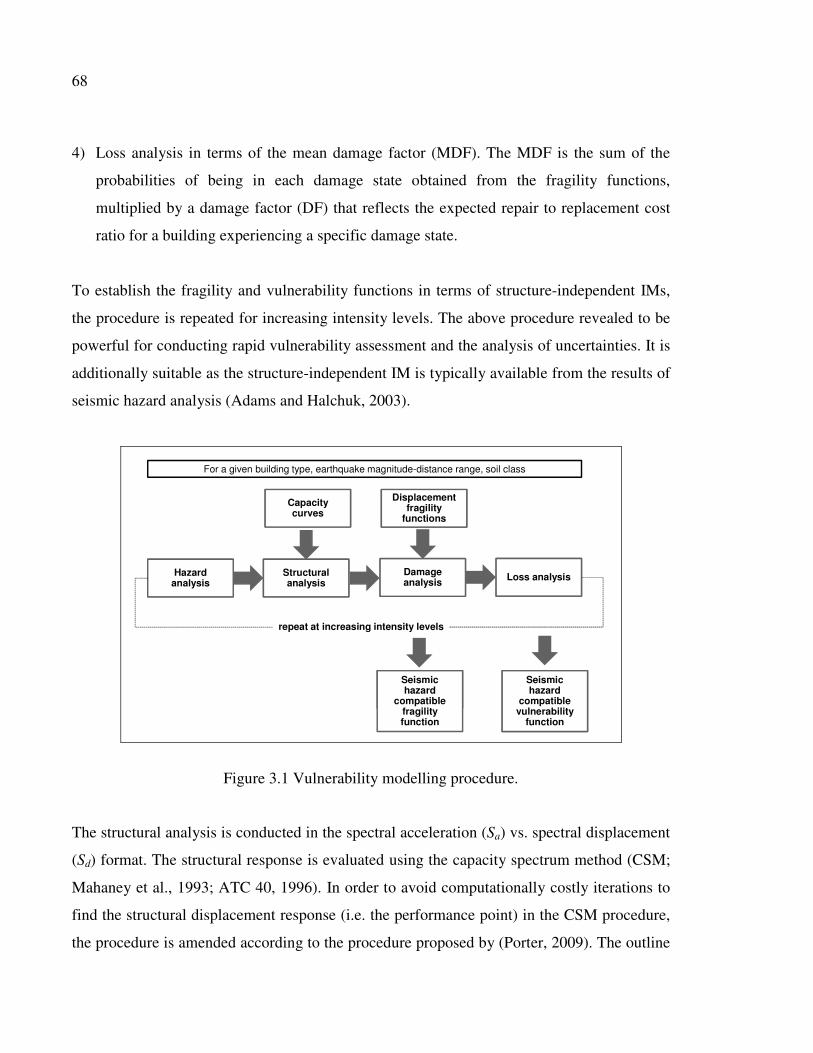
68
4) Loss analysis in terms of the mean damage factor (MDF). The MDF is the sum of the
probabilities of being in each damage state obtained from the fragility functions,
multiplied by a damage factor (DF) that reflects the expected repair to replacement cost
ratio for a building experiencing a specific damage state.
To establish the fragility and vulnerability functions in terms of structure-independent IMs,
the procedure is repeated for increasing intensity levels. The above procedure revealed to be
powerful for conducting rapid vulnerability assessment and the analysis of uncertainties. It is
additionally suitable as the structure-independent IM is typically available from the results of
seismic hazard analysis (Adams and Halchuk, 2003).
Damage analysis Loss analysisHazard
analysisStructural analysis
repeat at increasing intensity levels
Capacity curves
Displacement fragility
functions
For a given building type, earthquake magnitude-distance range, soil class
Seismic hazard
compatible vulnerability
function
Seismic hazard
compatible fragility function
Figure 3.1 Vulnerability modelling procedure.
The structural analysis is conducted in the spectral acceleration (Sa) vs. spectral displacement
(Sd) format. The structural response is evaluated using the capacity spectrum method (CSM;
Mahaney et al., 1993; ATC 40, 1996). In order to avoid computationally costly iterations to
find the structural displacement response (i.e. the performance point) in the CSM procedure,
the procedure is amended according to the procedure proposed by (Porter, 2009). The outline

69
of the procedure is presented herein and more details of the computations can be found in the
Appendix-II.
In the CSM, the performance point is typically obtained based on the assumption that the
nonlinear response of the system can be modelled as a linear ESDOF with effective period
and effective damping. The effective damping of the system is proportional to the area
enclosed by the capacity curve to represent the hysteresis energy dissipation. The effective
period is assumed to be the secant period at which the seismic ground motion demand,
reduced for the equivalent damping, intersects the capacity curve.
The first step of the analysis is to determine the performance point on the spectral
acceleration Sa - spectral displacement Sd capacity curve for the considered earthquake
magnitude-distance scenario. The corresponding effective damping (�eff) is calculated from
Equation 3.1. The parameters are shown in Figure 3.2.
( )
2
4
eff ed ay
ay d dy
Areak
S S
Area S S S
ξ ξπ
� �= +
� �= −
(3.1)
where �e is the elastic damping ratio of the building, k is the degradation factor that
approximately account for the possible strength and stiffness degradation under cyclic
loading.
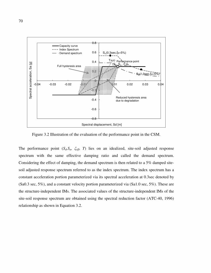
70
-0.8
-0.6
-0.4
-0.2
0
0.2
0.4
0.6
0.8
-0.04 -0.03 -0.02 -0.01 0 0.01 0.02 0.03 0.04
Spe
ctra
l acc
eler
atio
n, S
a [g
]
Spectral displacement, Sd [m]
Capacity curveIndex SpectrumDemand spectrum
(Sd ,Sa,, �eff)
Sa(1.0sec,���5%)
Sa(0.3sec,���5%)
Performance point
Full hysteresis area
Reduced hysteresis area due to degradation
TAVD
Figure 3.2 Illustration of the evaluation of the performance point in the CSM.
The performance point (Sd,Sa, �eff, T) lies on an idealized, site-soil adjusted response
spectrum with the same effective damping ratio and called the demand spectrum.
Considering the effect of damping, the demand spectrum is then related to a 5% damped site-
soil adjusted response spectrum referred to as the index spectrum. The index spectrum has a
constant acceleration portion parameterized via its spectral acceleration at 0.3sec denoted by
(Sa0.3 sec, 5%), and a constant velocity portion parameterized via (Sa1.0 sec, 5%). These are
the structure-independent IMs. The associated values of the structure-independent IMs of the
site-soil response spectrum are obtained using the spectral reduction factor (ATC-40, 1996)
relationship as shown in Equation 3.2.
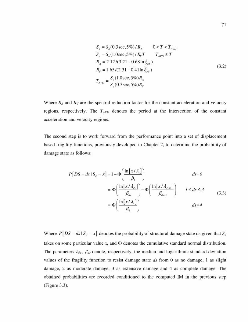
71
(0.3sec,5%) / 0
(1.0sec,5%) /
2.12 /(3.21 0.68ln )
1.65 /(2.31 0.41ln )
(1.0sec,5%)(0.3sec,5%)
a a A AVD
a a V AVD
A eff
V eff
a AAVD
a V
S S R T T
S S R T T T
R
R
S RT
S R
ξ
ξ
= < <
= ≤
= −
= −
=
(3.2)
Where RA and RV are the spectral reduction factor for the constant acceleration and velocity
regions, respectively. The TAVD denotes the period at the intersection of the constant
acceleration and velocity regions.
The second step is to work forward from the performance point into a set of displacement
based fragility functions, previously developed in Chapter 2, to determine the probability of
damage state as follows:
[ ][ ]
[ ] [ ]
[ ]
1
1
1
1
4
ln /| 1
ln / ln /
ln /
d
ds ds
ds ds
xP DS ds S x ds=0
x x = 1 ds 3
x =
λ
β
λ λ
β β
λ
β
+
+
� �= = = − Φ
� �� � � �
Φ − Φ ≤ ≤ � � � �
Φ4
ds=4
� � � �
(3.3)
Where [ ]| dP DS ds S x= = denotes the probability of structural damage state ds given that Sd
takes on some particular value x, and � denotes the cumulative standard normal distribution.
The parameters �ds , �ds denote, respectively, the median and logarithmic standard deviation
values of the fragility function to resist damage state ds from 0 as no damage, 1 as slight
damage, 2 as moderate damage, 3 as extensive damage and 4 as complete damage. The
obtained probabilities are recorded conditioned to the computed IM in the previous step
(Figure 3.3).
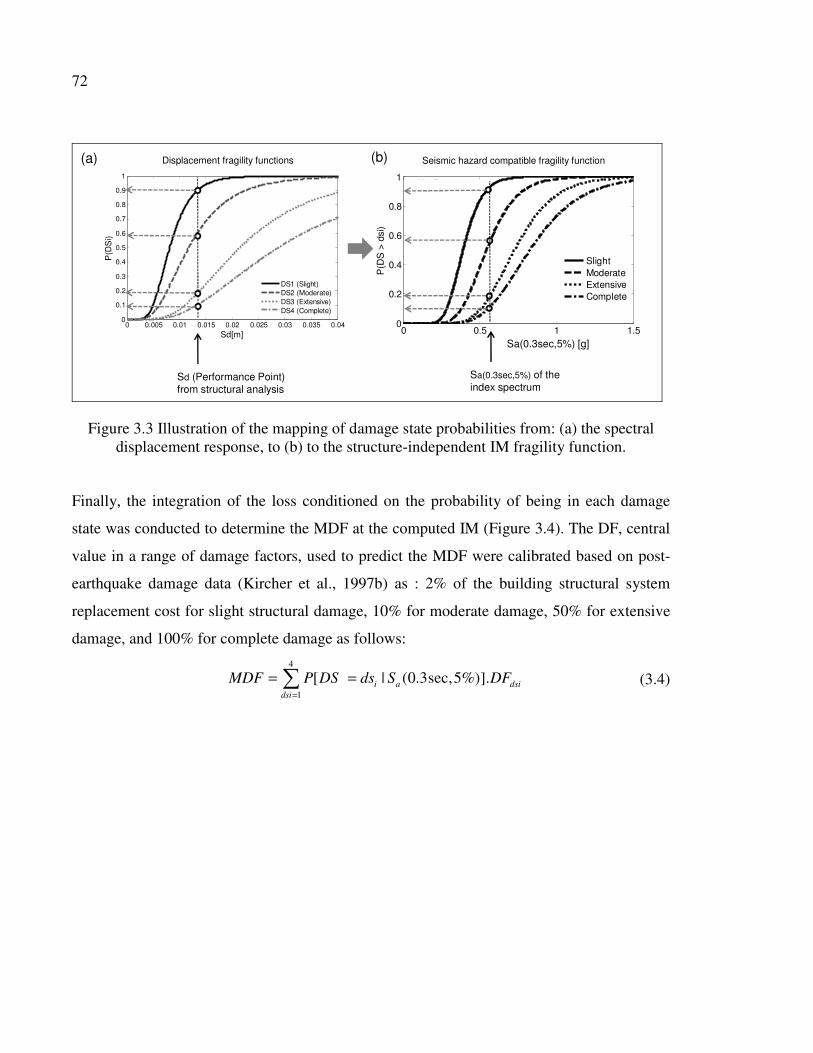
72
0 0.005 0.01 0.015 0.02 0.025 0.03 0.035 0.040
0.1
0.2
0.3
0.4
0.5
0.6
0.7
0.8
0.9
1
Sd[m]
P(D
Si)
DS1 (Slight)DS2 (Moderate)DS3 (Extensive)DS4 (Complete)
0 0.5 1 1.50
0.2
0.4
0.6
0.8
1
Sa(0.3sec,5%) [g]
P(D
S >
dsi
)
SlightModerateExtensiveComplete
M = 7 ,R=20kmSoil-C
(a) (b)Displacement fragility functions Seismic hazard compatible fragility function
Sd (Performance Point) from structural analysis
Sa(0.3sec,5%) of the index spectrum
Sa(0.3sec,5%) [g]
Figure 3.3 Illustration of the mapping of damage state probabilities from: (a) the spectral displacement response, to (b) to the structure-independent IM fragility function.
Finally, the integration of the loss conditioned on the probability of being in each damage
state was conducted to determine the MDF at the computed IM (Figure 3.4). The DF, central
value in a range of damage factors, used to predict the MDF were calibrated based on post-
earthquake damage data (Kircher et al., 1997b) as : 2% of the building structural system
replacement cost for slight structural damage, 10% for moderate damage, 50% for extensive
damage, and 100% for complete damage as follows:
4
1
[ | (0.3sec,5%)].i a dsidsi
MDF P DS ds S DF=
= =� (3.4)
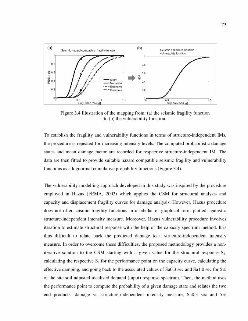
73
0 0.5 1 1.50
0.2
0.4
0.6
0.8
1
Sa(0.3sec,5%) [g]
P(D
S >
dsi
)
SlightModerateExtensiveComplete
M = 7 ,R=20kmSoil-C
0 0.5 1 1.50
0.2
0.4
0.6
0.8
1
Sa(0.3sec,5%) [g]
MD
F
M = 7 , R=20kmSoil-C
(a) (b)Seismic hazard compatible vulnerability function
Seismic hazard compatible fragility function
Figure 3.4 Illustration of the mapping from: (a) the seismic fragility function to (b) the vulnerability function.
To establish the fragility and vulnerability functions in terms of structure-independent IMs,
the procedure is repeated for increasing intensity levels. The computed probabilistic damage
states and mean damage factor are recorded for respective structure-independent IM. The
data are then fitted to provide suitable hazard compatible seismic fragility and vulnerability
functions as a lognormal cumulative probability functions (Figure 3.4).
The vulnerability modelling approach developed in this study was inspired by the procedure
employed in Hazus (FEMA, 2003) which applies the CSM for structural analysis and
capacity and displacement fragility curves for damage analysis. However, Hazus procedure
does not offer seismic fragility functions in a tabular or graphical form plotted against a
structure-independent intensity measure. Moreover, Hazus vulnerability procedure involves
iteration to estimate structural response with the help of the capacity spectrum method. It is
thus difficult to relate back the predicted damage to a structure-independent intensity
measure. In order to overcome these difficulties, the proposed methodology provides a non-
iterative solution to the CSM starting with a given value for the structural response Sd,
calculating the respective Sa for the performance point on the capacity curve, calculating the
effective damping, and going back to the associated values of Sa0.3 sec and Sa1.0 sec for 5%
of the site-soil-adjusted idealized demand (input) response spectrum. Then, the method uses
the performance point to compute the probability of a given damage state and relates the two
end products: damage vs. structure-independent intensity measure, Sa0.3 sec and 5%

74
damping in this case. The Hazus vulnerability procedure, on the other hand, starts from the
demand spectrum given Sa0.3 sec and Sa1.0 sec for 5% damping, calculating forward the
performance point with Sd and Sa for respective effective damping, which requires iterative
procedure, and then estimates the probability of the damage states. The computational
demands of the iteration can be significant for a large portfolio or a probabilistic risk
assessment, whereas having predefined fragility functions in terms of a structure-independent
IM greatly reduces the computational demands.
3.3 Scenario based vulnerability assessment
The procedure described above is applied to obtain sets of fragility and vulnerability
functions for typical stone masonry buildings in Old Quebec City. The earthquake scenarios
are generated based on two moment magnitudes, M6 and M7, and ranges of hypocentral
rupture distances (R) varying from 10 to 30 and from 20 to 60 km, respectively. The
idealized elastic response spectra is built using the Sa(0.3sec) and Sa(1.0sec) for 5% damping
computed with ground motion prediction equation (GMPE) for reference site-class C
developed by Atkinson and Boore (2006) for Eastern North America - AB06 (Figure 3.5).
Details of the AB06 GMPE can be found in Appendix-III.
0
0.2
0.4
0.6
0.8
1
1.2
0 0.5 1 1.5 2
Spe
ctra
l acc
eler
atio
n S
a [g
]
Period T [sec]
M6,R10
M6,R15
M6,R20
M6,R30
M7,R20
M7,R30
M7,R40
M7,R60
Soil Class-C
Figure 3.5 Idealized response spectra for scenario earthquakes using Sa0.3 sec and Sa1.0 sec values from AB06 GMPE. M is moment magnitude and R is hypocentral distance in km.
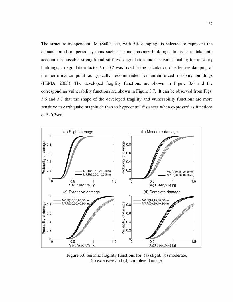
75
The structure-independent IM (Sa0.3 sec, with 5% damping) is selected to represent the
demand on short period systems such as stone masonry buildings. In order to take into
account the possible strength and stiffness degradation under seismic loading for masonry
buildings, a degradation factor k of 0.2 was fixed in the calculation of effective damping at
the performance point as typically recommended for unreinforced masonry buildings
(FEMA, 2003). The developed fragility functions are shown in Figure 3.6 and the
corresponding vulnerability functions are shown in Figure 3.7. It can be observed from Figs.
3.6 and 3.7 that the shape of the developed fragility and vulnerability functions are more
sensitive to earthquake magnitude than to hypocentral distances when expressed as functions
of Sa0.3sec.
0 0.5 1 1.50
0.2
0.4
0.6
0.8
1
Sa(0.3sec,5%) [g]
Pro
babi
lity
of d
amag
e
0 0.5 1 1.50
0.2
0.4
0.6
0.8
1
Sa(0.3sec,5%) [g]
Pro
babi
lity
of d
amag
e
0 0.5 1 1.50
0.2
0.4
0.6
0.8
1
Sa(0.3sec,5%) [g]
Pro
babi
lity
of d
amag
e
0 0.5 1 1.50
0.2
0.4
0.6
0.8
1
Sa(0.3sec,5%) [g]
Pro
babi
lity
of d
amag
e
(a) Slight damage
(d) Complete damage(c) Extensive damage
(b) Moderate damage
M6,R(10,15,20,30km)M7,R(20,30,40,60km)
M6,R(10,15,20,30km)M7,R(20,30,40,60km)
M6,R(10,15,20,30km)M7,R(20,30,40,60km)
M6,R(10,15,20,30km)M7,R(20,30,40,60km)
Figure 3.6 Seismic fragility functions for: (a) slight, (b) moderate, (c) extensive and (d) complete damage.
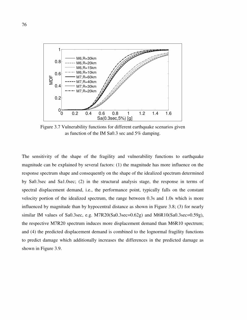
76
0 0.2 0.4 0.6 0.8 1 1.2 1.4 1.60
0.2
0.4
0.6
0.8
1
Sa(0.3sec,5%) [g]
MD
F
M6,R=30kmM6,R=20kmM6,R=15kmM6,R=10kmM7,R=60kmM7,R=40kmM7,R=30kmM7,R=20km
Figure 3.7 Vulnerability functions for different earthquake scenarios given as function of the IM Sa0.3 sec and 5% damping.
The sensitivity of the shape of the fragility and vulnerability functions to earthquake
magnitude can be explained by several factors: (1) the magnitude has more influence on the
response spectrum shape and consequently on the shape of the idealized spectrum determined
by Sa0.3sec and Sa1.0sec; (2) in the structural analysis stage, the response in terms of
spectral displacement demand, i.e., the performance point, typically falls on the constant
velocity portion of the idealized spectrum, the range between 0.3s and 1.0s which is more
influenced by magnitude than by hypocentral distance as shown in Figure 3.8; (3) for nearly
similar IM values of Sa0.3sec, e.g. M7R20(Sa0.3sec=0.62g) and M6R10(Sa0.3sec=0.59g),
the respective M7R20 spectrum induces more displacement demand than M6R10 spectrum;
and (4) the predicted displacement demand is combined to the lognormal fragility functions
to predict damage which additionally increases the differences in the predicted damage as
shown in Figure 3.9.
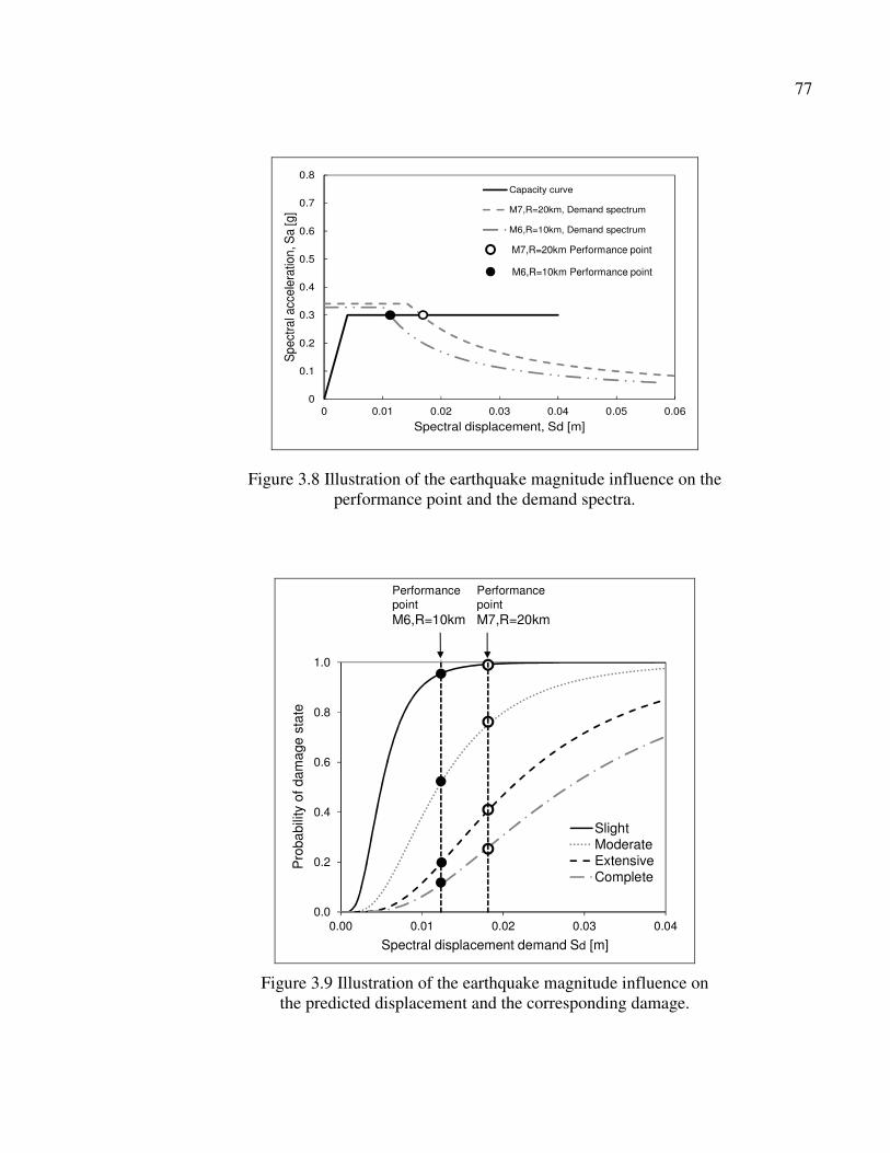
77
0
0.1
0.2
0.3
0.4
0.5
0.6
0.7
0.8
0 0.01 0.02 0.03 0.04 0.05 0.06
Spe
ctra
l acc
eler
atio
n, S
a [g
]
Spectral displacement, Sd [m]
Capacity curve
M7,R=20km, Demand spectrum
M6,R=10km, Demand spectrum
M7,R=20km Performance point
M6,R=10km Performance point
Figure 3.8 Illustration of the earthquake magnitude influence on the performance point and the demand spectra.
0.0
0.2
0.4
0.6
0.8
1.0
0.00 0.01 0.02 0.03 0.04
Pro
babi
lity
of d
amag
e st
ate
Spectral displacement demand Sd [mm]
SlightModerateExtensiveComplete
Performance point M6,R=10km
Performance pointM7,R=20km
Spectral displacement demand Sd [m]
Figure 3.9 Illustration of the earthquake magnitude influence on the predicted displacement and the corresponding damage.
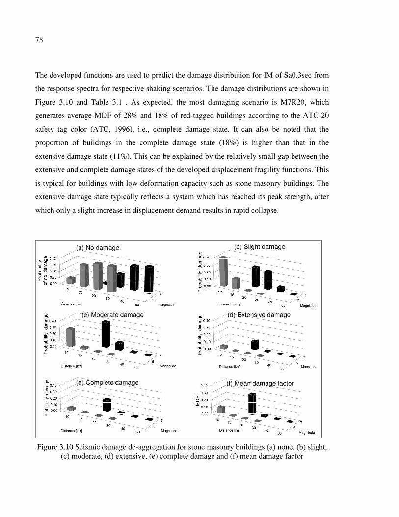
78
The developed functions are used to predict the damage distribution for IM of Sa0.3sec from
the response spectra for respective shaking scenarios. The damage distributions are shown in
Figure 3.10 and Table 3.1 . As expected, the most damaging scenario is M7R20, which
generates average MDF of 28% and 18% of red-tagged buildings according to the ATC-20
safety tag color (ATC, 1996), i.e., complete damage state. It can also be noted that the
proportion of buildings in the complete damage state (18%) is higher than that in the
extensive damage state (11%). This can be explained by the relatively small gap between the
extensive and complete damage states of the developed displacement fragility functions. This
is typical for buildings with low deformation capacity such as stone masonry buildings. The
extensive damage state typically reflects a system which has reached its peak strength, after
which only a slight increase in displacement demand results in rapid collapse.
(a) No damage (b) Slight damage
(c) Moderate damage (d) Extensive damage
(e) Complete damage (f) Mean damage factor
Figure 3.10 Seismic damage de-aggregation for stone masonry buildings (a) none, (b) slight, (c) moderate, (d) extensive, (e) complete damage and (f) mean damage factor

79
Table 3.1 Probability of damage distribution for different M and R for stone masonry buildings.
Probability of no damage Distance (R) [km]
Magnitude (M) 10 15 20 30 40 60
6 0.20 0.84 0.99 1.00
7 0.03 0.50 0.93 1.00
Probability of slight damage Distance (R) [km]
Magnitude (M) 10 15 20 30 40 60
6 0.45 0.14 0.01 0.00
7 0.28 0.25 0.06 0.00
Probability of moderate damage Distance (R) [km]
Magnitude (M) 10 15 20 30 40 60
6 0.27 0.02 0.00 0.00
7 0.39 0.11 0.01 0.00
Probability of Extensive damage Distance (R) [km]
Magnitude (M) 10 15 20 30 40 60
6 0.04 0.00 0.00 0.00
7 0.11 0.01 0.00 0.00
Probability of Complete damage Distance (R) [km]
Magnitude (M) 10 15 20 30 40 60
6 0.07 0.00 0.00 0.00
7 0.18 0.01 0.00 0.00
Mean damage factor (MDF) Distance (R) [km]
Magnitude (M) 10 15 20 30 40 60
6 0.11 0.01 0.00 0.00
7 0.28 0.03 0.00 0.00
80
3.4 Summary and conclusions
A robust analytical procedure for the development of seismic hazard compatible fragility and
vulnerability functions of stone masonry buildings is presented. The vulnerability analysis
procedure is a subsequent step of the development of the two main inputs for the
vulnerability analysis: (1) capacity curves that characterize the nonlinear behaviour of the
existing stone masonry buildings and (2) displacement based fragility functions that represent
the probability of exceedance of specified damage state under various levels of structural
response. These two inputs are convolved with response spectra to estimate the structural
damage to buildings for a series of earthquake magnitude-distance combinations. The results
are sets of seismic hazard compatible vulnerability functions that can be directly used with
seismic hazard analysis output that is typically presented in terms of structure-independent
intensity measure (IM). Therefore, the procedure revealed to be powerful for conducting
rapid vulnerability assessment of building classes. Moreover, the procedure leads to the
reduction of the computational time of vulnerability assessment when a sensitivity analysis is
to be conducted. A scenario-based vulnerability assessment of stone masonry building was
also conducted as an example to demonstrate the capacities of the procedure. As expected,
the most damaging scenario was M7R20, which generates average MDF of 28% and 18% of
red-tagged buildings, i.e., complete damage. The presented vulnerability assessment
procedure will be used to develop vulnerability functions for other buildings types present in
Old Québec City with proper specific capacity and displacement based fragility functions
(Chapter 5).
CHAPTER 4
SENSITIVITY ANALYSIS ON VULNERABILITY MODELLING
4.1 Introduction
Vulnerability modeling is usually constrained by limited information and knowledge and
uncertainties arise throughout the assessment process. One of the most important aspects in
development of a seismic vulnerability model is to identify, quantify and incorporate the
uncertainties associated with each of the input parameter (Crowley et al., 2005).
The objective of this chapter is to investigate the uncertainties in analytical vulnerability
modelling of stone masonry buildings. The conducted sensitivity analyses will contribute to
the identification of critical parameters with significant impact on the damage estimates.
The following parameters were considered in the sensitivity analyses: (1) structural
parameters: yield acceleration Say of the capacity curve, elastic damping ratio e, and
degradation factor k ; (2) damage parameters: displacement fragility functions defined by
median � and standard deviation � ; and (3) loss parameters: repair cost ratio DF. A base case
scenario was run first with default parameters used for the development of the vulnerability
function for the low-rise stone masonry building. For each parameter, a set of increments was
considered next in the range of ±25% and ±50% and with respect to the base case scenario.
The vulnerability functions were then developed by varying the values of the considered
parameter and leaving the remaining parameters unchanged, i.e., with values equal to those
of the base case scenario. The respective sensitivity was determined by measuring the
deviation from the base-case scenario. The absolute value of the difference from the base-
case scenario MDF (swing) is retained as a measure of the sensitivity (Porter et al., 2002),
where parameters that have larger swing have more impact on the final MDF results and are
considered critical for the analytical vulnerability modeling. In addition, three levels of
structure-independent IMs were considered, IM (Sa0.3 sec) = 0.4g, 0.5g and 0.6g, to study
the impact of the seismic intensity on the sensitivity to each of the considered parameters.
82
4.2 Variation in structural parameters
The investigate structural parameters are: (1) the yield acceleration of the capacity curves Say,
(2) the elastic damping ratio �e and (3) the structural degradation factor k.
Capacity curve reflects the lateral resistance envelope for an ESDOF representation of a
building under seismic loading. The simplified mechanical model presented in chapter 2 is
used for the development of ideal elasto-plastic capacity curves, which considers variable
material properties (e.g., compressive strength, shear strength). The median capacity curve
with Say=0.3g is selected for the base-case scenario, and the yield spectral acceleration is
varied in the predefined increments of ±25% and ±50%.
The CSM adopted for the structural analysis assumes a simple ESDOF system with
equivalent effective damping, defined as a sum of the elastic damping and the hysteretic
damping (ATC, 1996). The elastic viscous damping considers the energy dissipated by the
structure in the elastic range. This dissipation can be attributed to various mechanisms such
as interaction between structural and non-structural elements, small cracking effects during
elastic loading. The base-case scenario elastic damping is fixed to 10% (FEMA, 2003;
Benedetti et al., 1998).
The hysteretic damping reflects the energy dissipated under cyclic earthquake loading, i.e.,
area enclosed by the hysteresis loop under the capacity curve, and is dependent on the
response amplitude (ATC, 1996). This considers potential degradation of the structural
energy-absorption capacity during the cyclic earthquake loading defined by a degradation
factor, k, which is a function of the strong motion duration and the structural system. The
assumed degradation factor for the base-case scenario is k=0.2 (FEMA, 2003). Table 4.1
shows the investigated variations in the structural parameters.
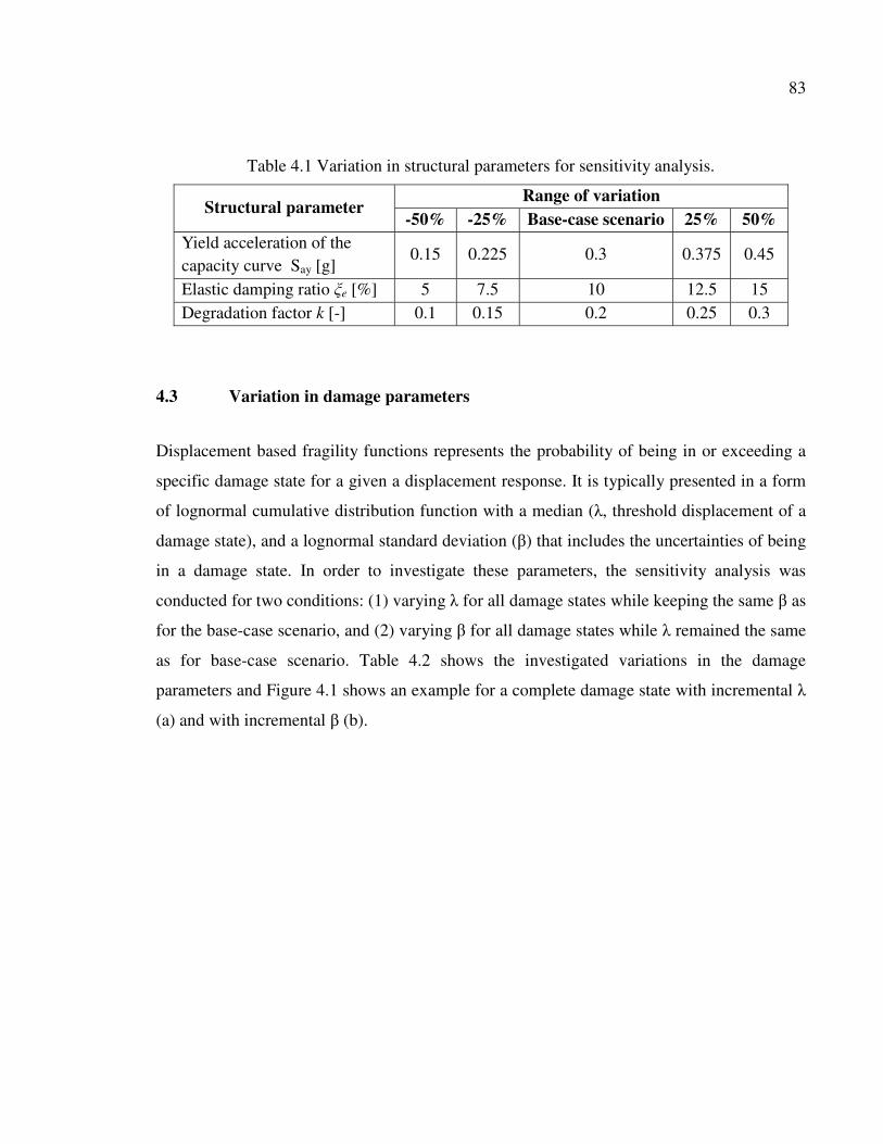
83
Table 4.1 Variation in structural parameters for sensitivity analysis.
Structural parameter Range of variation
-50% -25% Base-case scenario 25% 50% Yield acceleration of the capacity curve Say [g]
0.15 0.225 0.3 0.375 0.45
Elastic damping ratio �e [%] 5 7.5 10 12.5 15 Degradation factor k [-] 0.1 0.15 0.2 0.25 0.3
4.3 Variation in damage parameters
Displacement based fragility functions represents the probability of being in or exceeding a
specific damage state for a given a displacement response. It is typically presented in a form
of lognormal cumulative distribution function with a median (�, threshold displacement of a
damage state), and a lognormal standard deviation (�) that includes the uncertainties of being
in a damage state. In order to investigate these parameters, the sensitivity analysis was
conducted for two conditions: (1) varying � for all damage states while keeping the same � as
for the base-case scenario, and (2) varying � for all damage states while � remained the same
as for base-case scenario. Table 4.2 shows the investigated variations in the damage
parameters and Figure 4.1 shows an example for a complete damage state with incremental �
(a) and with incremental � (b).
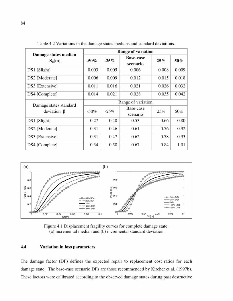
84
Table 4.2 Variations in the damage states medians and standard deviations.
Damage states median Sd[m]
Range of variation
-50% -25% Base-case scenario
25% 50%
DS1 [Slight] 0.003 0.005 0.006 0.008 0.009
DS2 [Moderate] 0.006 0.009 0.012 0.015 0.018
DS3 [Extensive] 0.011 0.016 0.021 0.026 0.032
DS4 [Complete] 0.014 0.021 0.028 0.035 0.042
Damage states standard deviation �
Range of variation
-50% -25% Base-case scenario
25% 50%
DS1 [Slight] 0.27 0.40 0.53 0.66 0.80
DS2 [Moderate] 0.31 0.46 0.61 0.76 0.92
DS3 [Extensive] 0.31 0.47 0.62 0.78 0.93
DS4 [Complete] 0.34 0.50 0.67 0.84 1.01
0 0.02 0.04 0.06 0.08 0.10
0.2
0.4
0.6
0.8
1
Sd[m]
P(D
Si |
Sd)
50% DS425% DS4DS4-25% DS4-50% DS4
(a)
0 0.02 0.04 0.06 0.08 0.10
0.2
0.4
0.6
0.8
1
Sd[m]
P(D
Si |
Sd)
50% DS425% DS4DS4-25% DS4-50% DS4
(b)
Figure 4.1 Displacement fragility curves for complete damage state: (a) incremental median and (b) incremental standard deviation.
4.4 Variation in loss parameters
The damage factor (DF) defines the expected repair to replacement cost ratios for each
damage state. The base-case scenario DFs are those recommended by Kircher et al. (1997b).
These factors were calibrated according to the observed damage states during past destructive
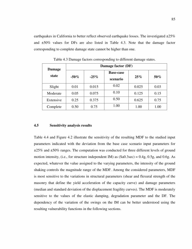
85
earthquakes in California to better reflect observed earthquake losses. The investigated ±25%
and ±50% values for DFs are also listed in Table 4.3. Note that the damage factor
corresponding to complete damage state cannot be higher than one.
Table 4.3 Damage factors corresponding to different damage states.
Damage
state
Damage factor (DF)
-50% -25% Base-case
scenario 25% 50%
Slight 0.01 0.015 0.02 0.025 0.03
Moderate 0.05 0.075 0.10 0.125 0.15
Extensive 0.25 0.375 0.50 0.625 0.75
Complete 0.50 0.75 1.00 1.00 1.00
4.5 Sensitivity analysis results
Table 4.4 and Figure 4.2 illustrate the sensitivity of the resulting MDF to the studied input
parameters indicated with the deviation from the base case scenario input parameters for
±25% and ±50% ranges. The computation was conducted for three different levels of ground
motion intensity, (i.e., for structure independent IM) as (Sa0.3sec) = 0.4g, 0.5g, and 0.6g. As
expected, whatever the value assigned to the varying parameters, the intensity of the ground
shaking controls the magnitude range of the MDF. Among the considered parameters, MDF
is most sensitive to the variations in structural parameters (shear and flexural strength of the
masonry that define the yield acceleration of the capacity curve) and damage parameters
(median and standard deviation of the displacement fragility curves). The MDF is moderately
sensitive to the values of the elastic damping, degradation parameter and the DF. The
dependency of the variation of the swings on the IM can be better understood using the
resulting vulnerability functions in the following sections.

86
Table 4.4 Sensitivity of the MDF to input parameters at different shaking intensities (IM).
IM (Sa0.3sec) 0.4g 0.5g 0.6g
MDF (base scenario) at the
respective IM 0.03 0.11 0.25
Parameters
Swing
(±25%)
Swing
(±50%)
Swing
(±25%)
Swing
(±50%)
Swing
(±25%)
Swing
(±50%)
Capacity curves (Say) 0.05 0.16 0.14 0.36 0.23 0.51
Fragility curves median (�) 0.06 0.15 0.16 0.33 0.25 0.49
Fragility curves Std. dev.(�) 0.05 0.09 0.10 0.18 0.10 0.18
Degradation factor (k) 0.02 0.04 0.06 0.12 0.10 0.21
Elastic damping (e) 0.02 0.04 0.06 0.12 0.10 0.20
Damage factors (DFs) 0.01 0.02 0.02 0.06 0.09 0.18
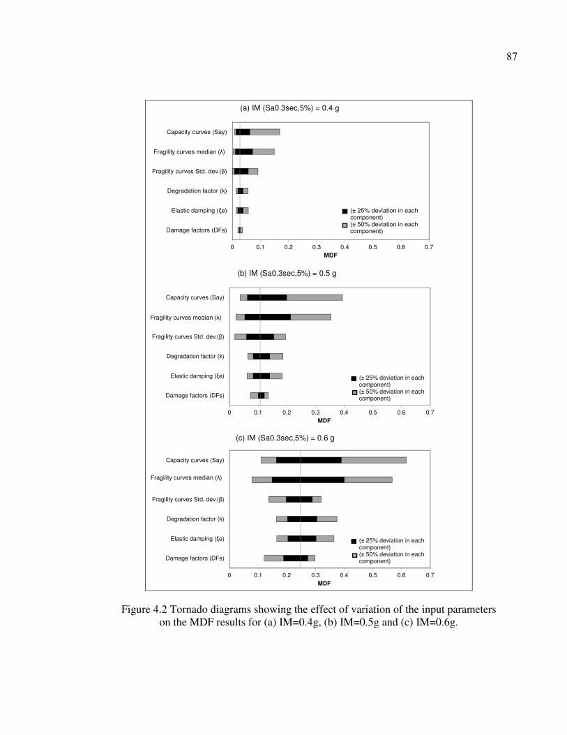
87
0 0.1 0.2 0.3 0.4 0.5 0.6 0.7
Damage factors (DFs)
Elastic damping (�e)
Degradation factor (k)
Fragility curves Std. dev.(�)
Fragility curves median (�)
Capacity curves (Say)
MDF
(� 25% deviation in each component)(� 50% deviation in each component)
0 0.1 0.2 0.3 0.4 0.5 0.6 0.7
Damage factors (DFs)
Elastic damping (�e)
Degradation factor (k)
Fragility curves Std. dev.(�)
Fragility curves median (�)
Capacity curves (Say)
MDF
(� 25% deviation in each component)(� 50% deviation in each component)
0 0.1 0.2 0.3 0.4 0.5 0.6 0.7
Damage factors (DFs)
Elastic damping (�e)
Degradation factor (k)
Fragility curves Std. dev.(�)
Fragility curves median (�)
Capacity curves (Say)
MDF
(� 25% deviation in each component)(� 50% deviation in each component)
(a) IM (Sa0.3sec,5%) = 0.4 g
(b) IM (Sa0.3sec,5%) = 0.5 g
(c) IM (Sa0.3sec,5%) = 0.6 g
Fragility curves median (�)
Fragility curves median (�)
Fragility curves median (�)
Figure 4.2 Tornado diagrams showing the effect of variation of the input parameters on the MDF results for (a) IM=0.4g, (b) IM=0.5g and (c) IM=0.6g.

88
4.6 Discussion of the sensitivity analysis results
4.6.1 Structural parameters
The sensitivity of the MDF to the variation in the yield acceleration of the capacity curve,
elastic damping and degradation parameter is illustrated in the vulnerability functions shown
in Figure 4.3a, b and c at increasing levels of seismic intensity. The sensitivity of MDF to the
variation of the structural parameters is mainly due to the difference in the predicted
displacement response, i.e., performance point, using CSM. The variation of the yield
acceleration has larger effect on the displacement response (performance point) than the
elastic damping and the degradation parameter. The displacement response at the
performance point is input to the displacement fragility functions, which give the probability
of the damage states for that displacement. Due to the log-normal definition of the fragility
functions, a slight increase in displacement demand leads to an amplified response in the
damage probabilities and consequently in the MDF. This illustrates the complex interaction
of the capacity and the displacement fragility functions for damage prediction.
0 0.5 1 1.50
0.2
0.4
0.6
0.8
1
Sa(0.3sec,5%) [g]
MD
F
+50% Say+25% SayBase Say-25% Say-50% Say
0 0.5 1 1.50
0.2
0.4
0.6
0.8
1
Sa(0.3sec,5%) [g]
MD
F
-50% base -25% base Base damping+25% base50%% base
0 0.5 1 1.50
0.2
0.4
0.6
0.8
1
Sa(0.3sec,5%) [g]
MD
F
-50% k-25% kBase k+25% k+50% k
(a) Yield acceleration Say
(c) Degradation factor k
(b) Elastic damping �e
-50% Say = 0.15g-25% Say = 0.23 gBase Say = 0.3g+ 25% Say = 0.38g+50% Say = 0.45g
-50% �e = 5%-25% �e = 7.5%Base �e = 10%+ 25% �e = 12.5%+50% �e = 15%
-50% k = 0.1-25% k = 0.15Base k = 0.2+ 25% k = 0.25+50% k = 0.3
Figure 4.3 Vulnerability functions for variation in input parameters: (a) yield acceleration, (b) elastic damping (c) degradation factor.
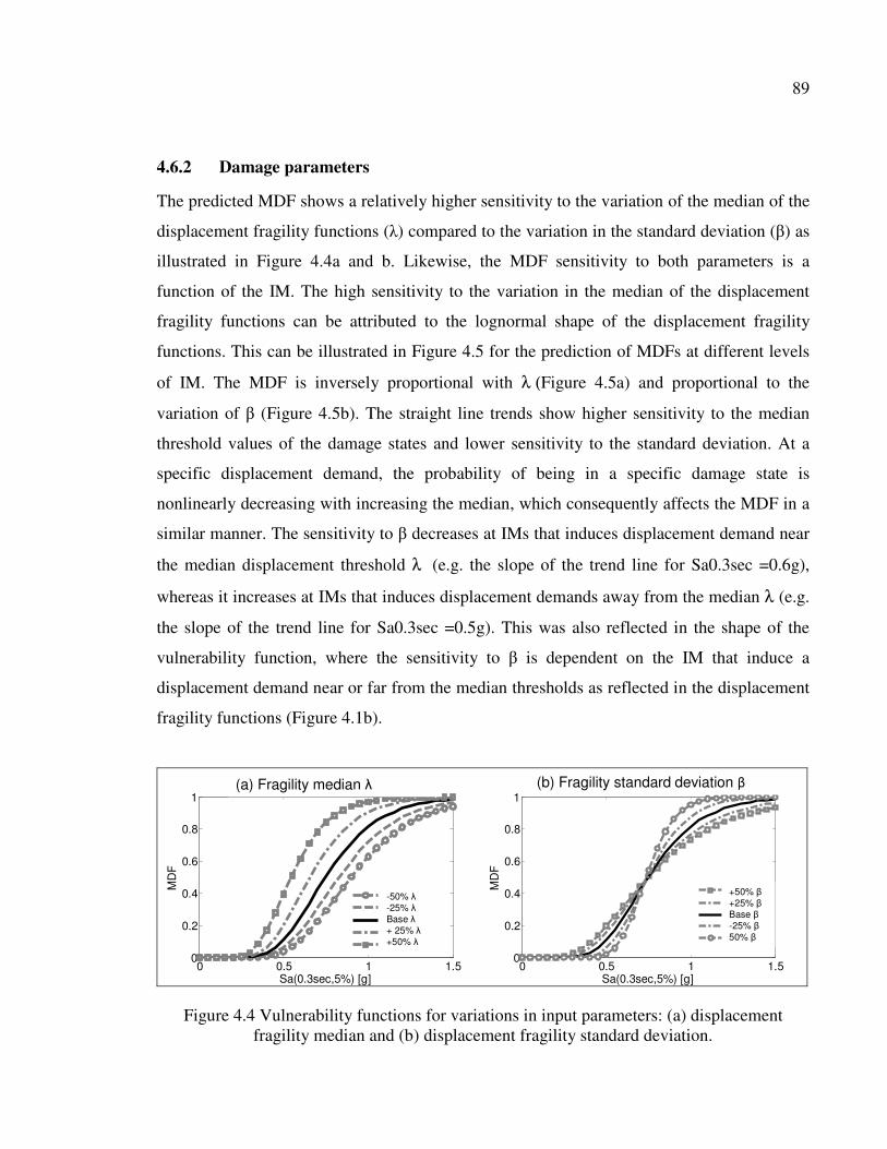
89
4.6.2 Damage parameters
The predicted MDF shows a relatively higher sensitivity to the variation of the median of the
displacement fragility functions (�) compared to the variation in the standard deviation (�) as
illustrated in Figure 4.4a and b. Likewise, the MDF sensitivity to both parameters is a
function of the IM. The high sensitivity to the variation in the median of the displacement
fragility functions can be attributed to the lognormal shape of the displacement fragility
functions. This can be illustrated in Figure 4.5 for the prediction of MDFs at different levels
of IM. The MDF is inversely proportional with λ (Figure 4.5a) and proportional to the
variation of � (Figure 4.5b). The straight line trends show higher sensitivity to the median
threshold values of the damage states and lower sensitivity to the standard deviation. At a
specific displacement demand, the probability of being in a specific damage state is
nonlinearly decreasing with increasing the median, which consequently affects the MDF in a
similar manner. The sensitivity to � decreases at IMs that induces displacement demand near
the median displacement threshold λ (e.g. the slope of the trend line for Sa0.3sec =0.6g),
whereas it increases at IMs that induces displacement demands away from the median λ (e.g.
the slope of the trend line for Sa0.3sec =0.5g). This was also reflected in the shape of the
vulnerability function, where the sensitivity to � is dependent on the IM that induce a
displacement demand near or far from the median thresholds as reflected in the displacement
fragility functions (Figure 4.1b).
0 0.5 1 1.50
0.2
0.4
0.6
0.8
1
Sa(0.3sec,5%) [g]
MD
F
-50% median-25% medianBase median+25% median+50% median
0 0.5 1 1.50
0.2
0.4
0.6
0.8
1
Sa(0.3sec,5%) [g]
MD
F
+50% beta+25% betaBase beta-25% beta-50% beta
(b) Fragility standard deviation �(a) Fragility median �
-50% �-25% � Base �+ 25% � +50% �
+50% �+25% �Base �-25% �50% �
Figure 4.4 Vulnerability functions for variations in input parameters: (a) displacement fragility median and (b) displacement fragility standard deviation.
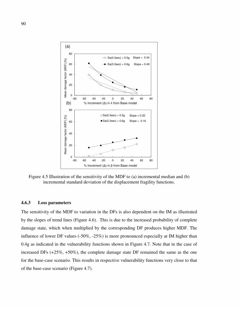
90
Slope = 0.34
Slope = 0.49
0
20
40
60
80
-80 -60 -40 -20 0 20 40 60 80
Mea
n da
mag
e fa
ctor
(M
DF
) [%
]
% Increment (�) in � from Base model
Sa(0.3sec) = 0.5g
Sa(0.3sec) = 0.6g
Slope = 0.20
Slope = 0.16
0
20
40
60
80
-80 -60 -40 -20 0 20 40 60 80
Mea
n da
mag
e fa
ctor
(M
DF
) [%
]
% Increment (�) in � from Base model
Sa(0.3sec) = 0.5g
Sa(0.3sec) = 0.6g
(a)
(b)
Figure 4.5 Illustration of the sensitivity of the MDF to (a) incremental median and (b) incremental standard deviation of the displacement fragility functions.
4.6.3 Loss parameters
The sensitivity of the MDF to variation in the DFs is also dependent on the IM as illustrated
by the slopes of trend lines (Figure 4.6). This is due to the increased probability of complete
damage state, which when multiplied by the corresponding DF produces higher MDF. The
influence of lower DF values (-50%, -25%) is more pronounced especially at IM higher than
0.4g as indicated in the vulnerability functions shown in Figure 4.7. Note that in the case of
increased DFs (+25%, +50%), the complete damage state DF remained the same as the one
for the base-case scenario. This results in respective vulnerability functions very close to that
of the base-case scenario (Figure 4.7).
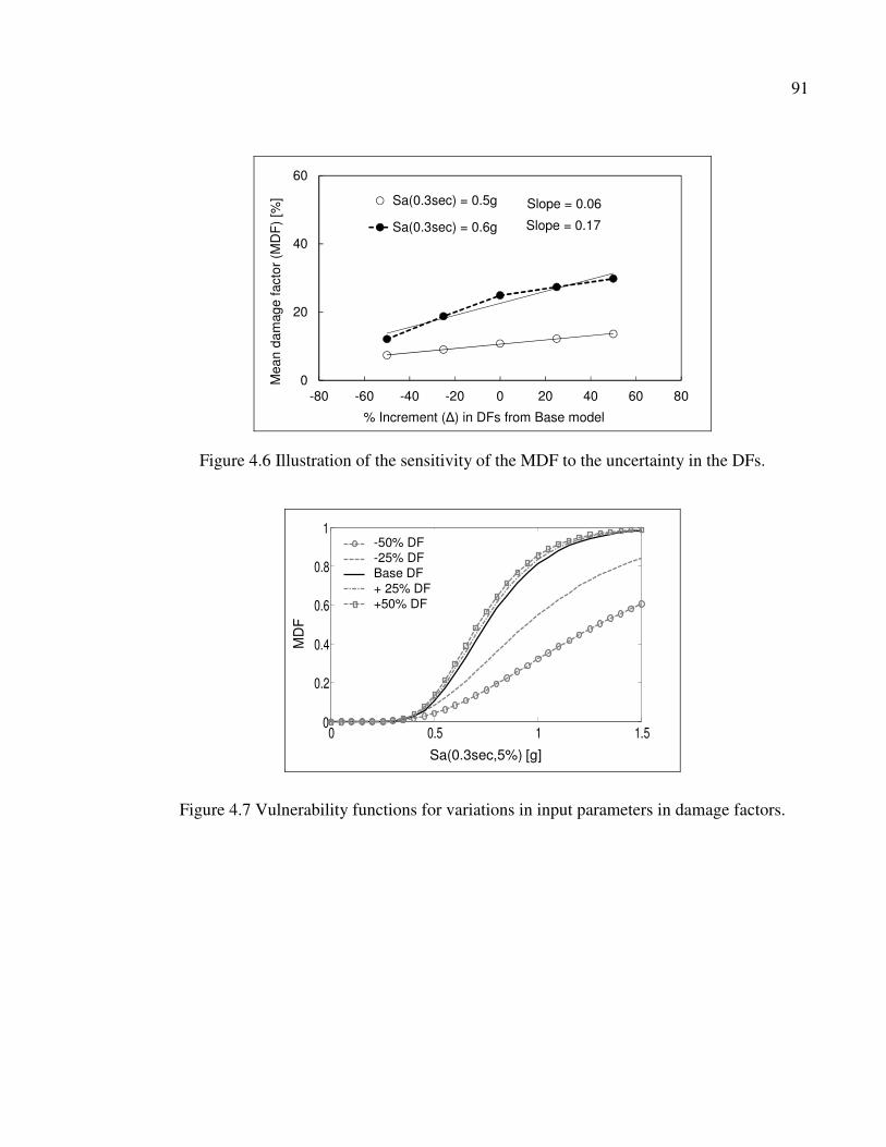
91
Slope = 0.06
Slope = 0.17
0
20
40
60
-80 -60 -40 -20 0 20 40 60 80
Mea
n da
mag
e fa
ctor
(M
DF
) [%
]
% Increment (�) in DFs from Base model
Sa(0.3sec) = 0.5g
Sa(0.3sec) = 0.6g
Figure 4.6 Illustration of the sensitivity of the MDF to the uncertainty in the DFs.
0 0.5 1 1.50
0.2
0.4
0.6
0.8
1
Sa(0.3sec,5%) [g]
-50% DFs-25% DFsBase DFs+25% DFs+50% DFs
-50% DF-25% DFBase DF+ 25% DF+50% DF
MD
F
Sa(0.3sec,5%) [g]
Figure 4.7 Vulnerability functions for variations in input parameters in damage factors.
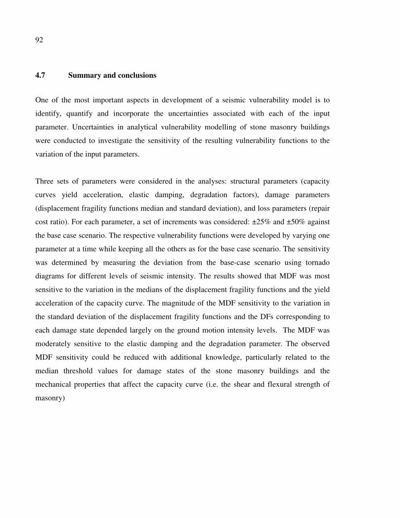
92
4.7 Summary and conclusions
One of the most important aspects in development of a seismic vulnerability model is to
identify, quantify and incorporate the uncertainties associated with each of the input
parameter. Uncertainties in analytical vulnerability modelling of stone masonry buildings
were conducted to investigate the sensitivity of the resulting vulnerability functions to the
variation of the input parameters.
Three sets of parameters were considered in the analyses: structural parameters (capacity
curves yield acceleration, elastic damping, degradation factors), damage parameters
(displacement fragility functions median and standard deviation), and loss parameters (repair
cost ratio). For each parameter, a set of increments was considered: ±25% and ±50% against
the base case scenario. The respective vulnerability functions were developed by varying one
parameter at a time while keeping all the others as for the base case scenario. The sensitivity
was determined by measuring the deviation from the base-case scenario using tornado
diagrams for different levels of seismic intensity. The results showed that MDF was most
sensitive to the variation in the medians of the displacement fragility functions and the yield
acceleration of the capacity curve. The magnitude of the MDF sensitivity to the variation in
the standard deviation of the displacement fragility functions and the DFs corresponding to
each damage state depended largely on the ground motion intensity levels. The MDF was
moderately sensitive to the elastic damping and the degradation parameter. The observed
MDF sensitivity could be reduced with additional knowledge, particularly related to the
median threshold values for damage states of the stone masonry buildings and the
mechanical properties that affect the capacity curve (i.e. the shear and flexural strength of
masonry)

CHAPTER 5
SEISMIC RISK ASSESSMENT OF EXISTING BUILDINGS IN OLD QUÉBEC CITY
5.1 Introduction
This chapter presents the results of an analytical seismic risk assessment study of the Old
Québec City, Canada. The framework of seismic risk assessment consists of three
components: hazard, inventory, and vulnerability of the inventory given the seismic hazard.
The vulnerability modeling consists of the development of analytical seismic fragility and
vulnerability functions using the procedure presented in chapter 3. The analytical functions
are conditioned to a structure-independent hazard intensity measure (IM), e.g. spectral
acceleration at a particular period. The study include an inventory analysis of some 1220
existing buildings, mainly pre-code unreinforced brick and stone masonry. The distribution
of the potential damage is evaluated for a scenario M6.2R15 event which corresponds to a
probability of exceedance of 2% in 50 years (Adams and Halchuk, 2003). The resulting
distribution of damage for the selected seismic scenario is presented.
5.2 Seismic risk assessment input models
The analytical seismic risk assessment framework for existing buildings requires three input
models: (1) buildings inventory model of existing buildings types and classification of
buildings according to construction material, height and design level, (2) seismic hazard
model using a ground-motion prediction equation compatible to the seismo-tectonic settings
at the study region to estimate shaking intensity in terms of a structure-independent IM, (3)
vulnerability model represented as seismic hazard compatible fragility functions in terms of
structure-independent intensity measure (IM) which in this study is Sa(0.3sec). The output is
the estimated damage magnitude and distribution. Figure 5.1 shows the flow chart for
seismic risk assessment methodology.
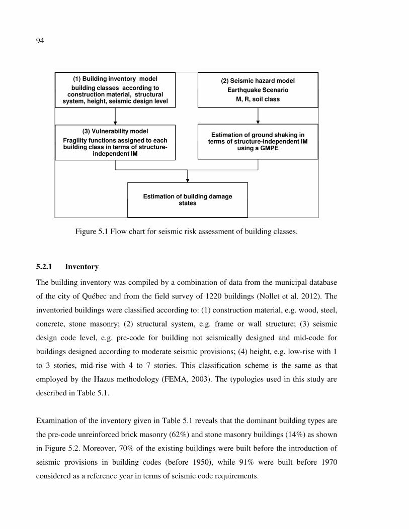
94
(1) Building inventory modelbuilding classes according to
construction material, structural system, height, seismic design level
(2) Seismic hazard model
Earthquake Scenario M, R, soil class
(3) Vulnerability model
Fragility functions assigned to each building class in terms of structure-
independent IM
Estimation of ground shaking in terms of structure-independent IM
using a GMPE
Estimation of building damage states
Figure 5.1 Flow chart for seismic risk assessment of building classes.
5.2.1 Inventory
The building inventory was compiled by a combination of data from the municipal database
of the city of Québec and from the field survey of 1220 buildings (Nollet et al. 2012). The
inventoried buildings were classified according to: (1) construction material, e.g. wood, steel,
concrete, stone masonry; (2) structural system, e.g. frame or wall structure; (3) seismic
design code level, e.g. pre-code for building not seismically designed and mid-code for
buildings designed according to moderate seismic provisions; (4) height, e.g. low-rise with 1
to 3 stories, mid-rise with 4 to 7 stories. This classification scheme is the same as that
employed by the Hazus methodology (FEMA, 2003). The typologies used in this study are
described in Table 5.1.
Examination of the inventory given in Table 5.1 reveals that the dominant building types are
the pre-code unreinforced brick masonry (62%) and stone masonry buildings (14%) as shown
in Figure 5.2. Moreover, 70% of the existing buildings were built before the introduction of
seismic provisions in building codes (before 1950), while 91% were built before 1970
considered as a reference year in terms of seismic code requirements.
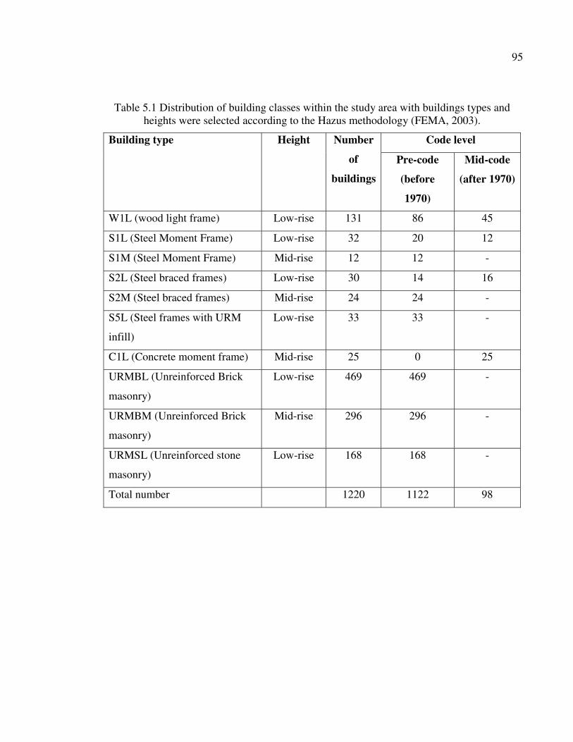
95
Table 5.1 Distribution of building classes within the study area with buildings types and heights were selected according to the Hazus methodology (FEMA, 2003).
Building type Height Number
of
buildings
Code level
Pre-code
(before
1970)
Mid-code
(after 1970)
W1L (wood light frame) Low-rise 131 86 45
S1L (Steel Moment Frame) Low-rise 32 20 12
S1M (Steel Moment Frame) Mid-rise 12 12 -
S2L (Steel braced frames) Low-rise 30 14 16
S2M (Steel braced frames) Mid-rise 24 24 -
S5L (Steel frames with URM
infill)
Low-rise 33 33 -
C1L (Concrete moment frame) Mid-rise 25 0 25
URMBL (Unreinforced Brick
masonry)
Low-rise 469 469 -
URMBM (Unreinforced Brick
masonry)
Mid-rise 296 296 -
URMSL (Unreinforced stone
masonry)
Low-rise 168 168 -
Total number 1220 1122 98
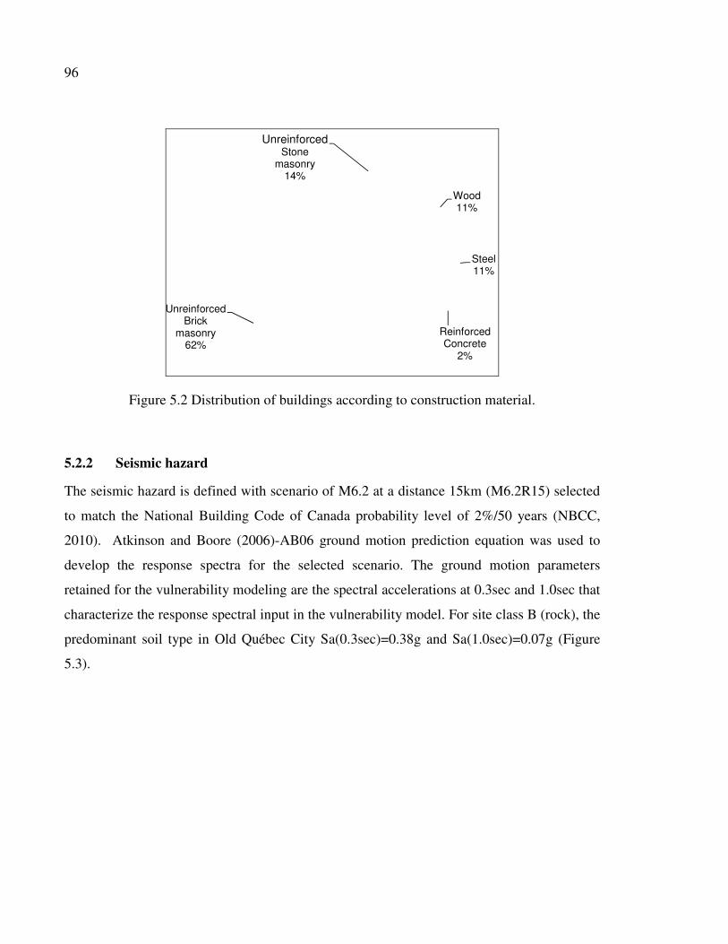
96
Wood11%
Steel11%
Reinforced Concrete
2%
Unreinforced Brick
masonry62%
Unreinforced Stone
masonry14%
Figure 5.2 Distribution of buildings according to construction material.
5.2.2 Seismic hazard
The seismic hazard is defined with scenario of M6.2 at a distance 15km (M6.2R15) selected
to match the National Building Code of Canada probability level of 2%/50 years (NBCC,
2010). Atkinson and Boore (2006)-AB06 ground motion prediction equation was used to
develop the response spectra for the selected scenario. The ground motion parameters
retained for the vulnerability modeling are the spectral accelerations at 0.3sec and 1.0sec that
characterize the response spectral input in the vulnerability model. For site class B (rock), the
predominant soil type in Old Québec City Sa(0.3sec)=0.38g and Sa(1.0sec)=0.07g (Figure
5.3).
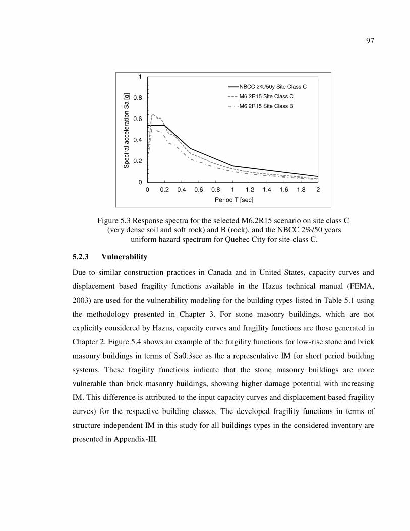
97
0
0.2
0.4
0.6
0.8
1
0 0.2 0.4 0.6 0.8 1 1.2 1.4 1.6 1.8 2
Spe
ctra
l acc
eler
atio
n S
a [g
]
Period T [sec]
NBCC 2%/50y Site Class C
M6.2R15 Site Class C
M6.2R15 Site Class B
Figure 5.3 Response spectra for the selected M6.2R15 scenario on site class C (very dense soil and soft rock) and B (rock), and the NBCC 2%/50 years
uniform hazard spectrum for Quebec City for site-class C.
5.2.3 Vulnerability
Due to similar construction practices in Canada and in United States, capacity curves and
displacement based fragility functions available in the Hazus technical manual (FEMA,
2003) are used for the vulnerability modeling for the building types listed in Table 5.1 using
the methodology presented in Chapter 3. For stone masonry buildings, which are not
explicitly considered by Hazus, capacity curves and fragility functions are those generated in
Chapter 2. Figure 5.4 shows an example of the fragility functions for low-rise stone and brick
masonry buildings in terms of Sa0.3sec as the a representative IM for short period building
systems. These fragility functions indicate that the stone masonry buildings are more
vulnerable than brick masonry buildings, showing higher damage potential with increasing
IM. This difference is attributed to the input capacity curves and displacement based fragility
curves) for the respective building classes. The developed fragility functions in terms of
structure-independent IM in this study for all buildings types in the considered inventory are
presented in Appendix-III.
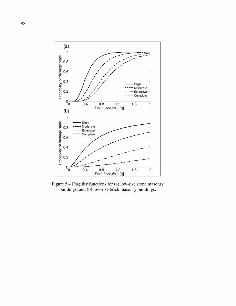
98
0 0.4 0.8 1.2 1.6 20
0.2
0.4
0.6
0.8
1
Sa(0.3sec,5%) [g]
Pro
babi
lity
of d
amag
e st
ate
SlightModerateExtensiveComplete
0 0.4 0.8 1.2 1.6 20
0.2
0.4
0.6
0.8
1
Sa(0.3sec,5%) [g]
Pro
babi
lity
of d
amag
e st
ate
SlightModerateExtensiveComplete
(a)
(b)
Figure 5.4 Fragility functions for (a) low-rise stone masonry buildings, and (b) low-rise brick masonry buildings.

99
5.3 Results
The potential damage for the considered M6.2R15 scenario is given in Figure 5.5. The total
number of buildings that will be subject to certain degree of damage is 369, or 30% of the
buildings. A summary of the proportion of buildings by construction material type and
damage states is shown Figure 5.6. Predictably, most of the expected damage will occur in
the pre-code stone and brick masonry buildings. Approximately 39% of the stone masonry
buildings (65 buildings out of 168) and 33% of the brick masonry buildings (252 buildings
out of 765) will suffer certain damage.
851
222
118
23 70
200
400
600
800
1000
None Slight Moderate Extensive Complete
Num
ber
of b
uild
ings
Figure 5.5 Total number of buildings in each damage state for a scenario event M6.2R15.
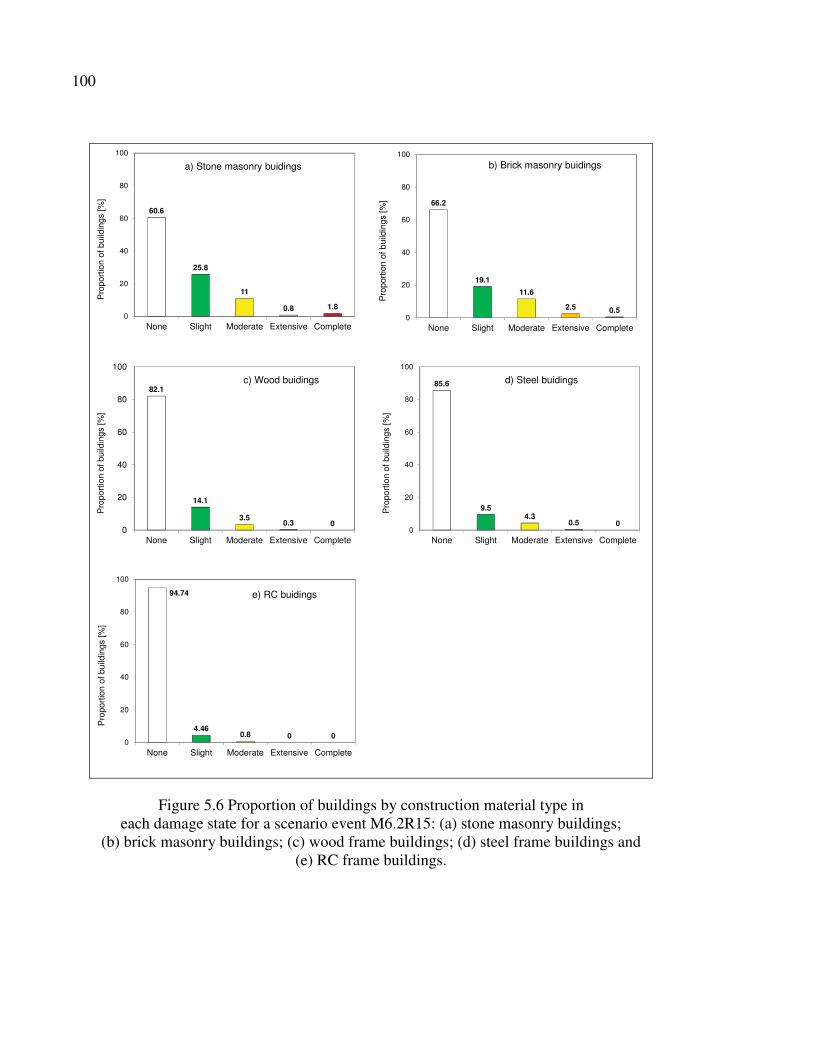
100
60.6
25.8
11
0.8 1.80
20
40
60
80
100
None Slight Moderate Extensive Complete
Pro
port
ion
of b
uild
ings
[%]
a) Stone masonry buidings
66.2
19.1
11.6
2.5 0.50
20
40
60
80
100
None Slight Moderate Extensive Complete
Pro
port
ion
of b
uild
ings
[%]
b) Brick masonry buidings
82.1
14.1
3.50.3 0
0
20
40
60
80
100
None Slight Moderate Extensive Complete
Pro
port
ion
of b
uild
ings
[%]
c) Wood buidings 85.6
9.54.3
0.5 00
20
40
60
80
100
None Slight Moderate Extensive Complete
Pro
port
ion
of b
uild
ings
[%]
d) Steel buidings
94.74
4.460.8 0 0
0
20
40
60
80
100
None Slight Moderate Extensive Complete
Pro
port
ion
of b
uild
ings
[%]
e) RC buidings
Figure 5.6 Proportion of buildings by construction material type in each damage state for a scenario event M6.2R15: (a) stone masonry buildings;
(b) brick masonry buildings; (c) wood frame buildings; (d) steel frame buildings and (e) RC frame buildings.
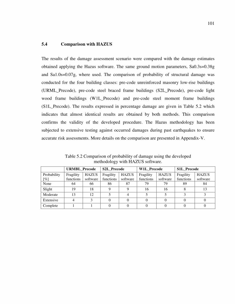
101
5.4 Comparison with HAZUS
The results of the damage assessment scenario were compared with the damage estimates
obtained applying the Hazus software. The same ground motion parameters, Sa0.3s=0.38g
and Sa1.0s=0.07g, where used. The comparison of probability of structural damage was
conducted for the four building classes: pre-code unreinforced masonry low-rise buildings
(URML_Precode), pre-code steel braced frame buildings (S2L_Precode), pre-code light
wood frame buildings (W1L_Precode) and pre-code steel moment frame buildings
(S1L_Precode). The results expressed in percentage damage are given in Table 5.2 which
indicates that almost identical results are obtained by both methods. This comparison
confirms the validity of the developed procedure. The Hazus methodology has been
subjected to extensive testing against occurred damages during past earthquakes to ensure
accurate risk assessments. More details on the comparison are presented in Appendix-V.
Table 5.2 Comparison of probability of damage using the developed methodology with HAZUS software.
URMBL_Precode S2L_Precode W1L_Precode S1L_Precode
Probability [%]
Fragility functions
HAZUS software
Fragility functions
HAZUS software
Fragility functions
HAZUS software
Fragility functions
HAZUS software
None 64 66 86 87 79 79 89 84
Slight 19 18 9 9 16 16 8 13
Moderate 13 12 5 4 5 5 3 3
Extensive 4 3 0 0 0 0 0 0
Complete 1 1 0 0 0 0 0 0

102
5.5 Summary and conclusions
A seismic risk assessment scenario of existing buildings inventory in Old Québec City was
conducted. Many of the buildings were built before the introduction of seismic provisions,
hence the need to predict their seismic performance. The assessment was performed for a
scenario event of magnitude 6.2 at distance 15km with a probability of exceedance of 2% in
50 years. The inventory consisted of 1220 buildings classified according to their material
type (e.g. concrete, wood, stone masonry), height (e.g. low, medium), and design level (e.g.
pre-code, recent code). The modeling procedure consisted of generation of a set of analytical
fragility functions in terms of a structure-independent intensity measure and respective to the
encountered building types. The study showed that most of the expected damage will be
concentrated in the old brick and stone masonry buildings, with 33% and 39% of damaged
buildings in the respective classes. The damage results are almost identical with those
obtained by applying the Hazus software for the same input parameters.
.

SUMMARY, CONCLUSIONS AND RECOMMENDATIONS
Summary
Earthquakes represent a major natural hazard that regularly impact the built environment in
seismic prone areas worldwide and cause considerable social and economic losses. Recent
earthquakes, e.g., 2009 L’Aquila earthquake in Italy and 2010 Christchurch earthquake in
New Zealand, showed that most of the damage and economic losses were related to old
vulnerable masonry buildings. The high losses incurred due to destructive earthquakes
promoted the need for assessment of the performance of existing buildings under potential
future earthquake events. This requires improved seismic vulnerability and risk assessment
tools needed to assist informed decision making with the objective to minimize potential
risks and to develop emergency response and recovery strategies.
In Eastern Canada, most of the existing buildings were built before the introduction of the
seismic provisions in building codes. In particular, pre-code masonry buildings types are
predominant in dense urban centers such as Québec City and Montreal in the Province of
Québec. The potential economic and social losses due to strong earthquake events can thus
be extensive. On the other hand, although masonry buildings represent major and most
vulnerable part of the existing building stock, less research was devoted to study the seismic
vulnerability of this type of buildings compared to other structural types, e.g. reinforced
concrete and steel buildings.
Many historic buildings in the old urban centers in Eastern Canada such as Old Québec City
are made of stone masonry and represent un-measurable architectural and cultural heritage.
These buildings were built to resist gravity loads only and generally offer poor resistance to
lateral seismic loads. The high seismic risk related to stone masonry buildings is even more
aggravated due to their location in densely populated urban centers in a way that the
consequences of failure of these structures tend to be severe with regards to human
casualties, heritage damage and economic losses. Seismic vulnerability assessment of stone
104
masonry buildings is therefore the first necessary step in developing seismic retrofitting and
pre-disaster mitigation plans for the older urban centers.
Typical seismic risk assessment studies on regional scale consist of three major components:
hazard, exposure, and vulnerability of the exposure with respect to the seismic hazard.
Seismic hazard defines the intensity of the expected earthquake motion at a particular
location over a given time period; exposure identifies the built environment (buildings and
infrastructures) in the area affected by the earthquake; and vulnerability refers to the
exposure susceptibility to earthquake impacts defined by the expected degree of damage and
loss that would result under different levels of seismic loading. The key component is the
vulnerability modelling. The vulnerability is typically presented with sets of fragility
functions describing the expected physical damage whereas economic losses are given by
vulnerability functions. The typical results of risk assessment comprise estimates of the
potential physical damage and direct economic losses.
The main objective of this study was to develop a set of probability-based analytical methods
and tools for efficient analysis of seismic vulnerability of stone masonry buildings with
systematic treatment of respective uncertainties. The specific objectives were to: (1) develop
fragility and vulnerability functions for stone masonry buildings; (2) quantify the
uncertainties in the vulnerability modelling and (3) apply the developed tools to evaluate the
seismic vulnerability and risk of stone masonry buildings and other buildings types in Old
Quebec City.
A simplified probabilistic analytical methodology for vulnerability modelling of stone
masonry building with systematic treatment of uncertainties that can be adapted to other
building types was developed in this study and presented in Chapter 2. Old Québec City was
selected as a study area representative for historical urban centers in Eastern Canada. The
first step in the methodology consisted of inventory of the existing stone masonry buildings
and characterization of representative typology. Respective building capacity model was
developed using a simplified mechanical model. Displacement based procedure was then
105
used to develop damage state fragility functions, based on drift thresholds of stone masonry
walls, assigned based on literature experimental data. A simplified probabilistic seismic
demand analysis was proposed to capture the combined uncertainty in capacity and demand
on the fragility curves. The generated displacement fragility functions were determined for
low-rise stone masonry buildings as functions of spectral displacement. The proposed
methodology can easily be applied to other building types provided that damage state drift
thresholds and material properties are available.
A robust analytical procedure for the development of seismic hazard compatible fragility and
vulnerability functions of stone masonry buildings was presented in Chapter 3. The two main
outputs that were developed in Chapter 2; the capacity curves and the displacement based
fragility functions; were convolved with response spectra to estimate the structural damage to
buildings for a series of earthquake magnitude-distance combinations in order to develop
seismic hazard compatible fragility and vulnerability functions in terms of a structure-
independent intensity measure (spectral acceleration). These functions can be directly used
with results of a seismic hazard analysis output that is typically presented in terms of
structure-independent intensity measure (IM). The procedure revealed to be effective for
conducting rapid vulnerability assessment of building classes by considerably reducing the
computational time. For a given building type, the developed procedure comprised the
following steps: (1) seismic hazard definition in terms of response spectra defined by
structure-independent intensity measures (e.g. spectral acceleration at a particular period);
(2) structural analysis on the pre-developed capacity curves to estimate the seismic demand;
(3) damage analysis using the pre-developed displacement based fragility functions for the
estimated seismic response and (4) loss analysis in terms of the mean damage factor (MDF)
which is obtained as a sum of the probabilities of being in each damage state obtained from
the fragility functions, multiplied by a damage factor (DF) that reflects the expected repair to
replacement cost ratio for a building experiencing a specific damage state.
106
Sensitivity analysis of uncertainties in analytical vulnerability modelling of stone masonry
buildings is presented in Chapter 4. The following parameters were varied: structural
parameters (capacity curves yield acceleration, elastic damping ratios, degradation factors),
damage parameters (displacement fragility functions median and standard deviation), and
loss parameters (repair cost ratio). For each parameter, a set of increments was considered.
First the vulnerability functions were developed for the base-case scenario. Then, the
vulnerability functions were developed by varying the considered parameter only and
keeping the remaining parameters constant. The sensitivity was determined comparing
deviations from the base-case scenario using tornado diagrams for different levels of seismic
intensity. The conducted sensitivity study revealed that largest part of MDF sensitivity is due
to the uncertainty in displacement fragility functions medians and the yield acceleration of
the capacity curve.
The proposed methodology was validated by conducting a scenario-based seismic risk
assessment of existing buildings in Old Québec City. The validation study is presented in
Chapter 5. The procedure for hazard compatible vulnerability modelling presented in Chapter
3 was used to develop seismic fragility functions in terms of spectral acceleration of existing
buildings inventory in Old Quebec City. The inventory consisted of 1220 buildings classified
according to their material type, height, and seismic design level. Many of these buildings
were built before the introduction of seismic provisions. The assessment was performed for a
scenario event of magnitude 6.2 at distance 15km with a probability of exceedance of 2% in
50 years. The study showed that most of the damage is expected to be concentrated in the old
brick and stone masonry buildings, with 33% and 39% of damaged buildings in the
respective classes. The damage results are almost identical with those obtained by applying
the Hazus software for the same input parameters.
107
Conclusions
A simplified probabilistic analytical methodology for vulnerability modelling of stone
masonry building with systematic treatment of uncertainties was developed in this study.
Respective building capacity model was developed using a simplified mechanical model.
Displacement based procedure was then used to develop damage state fragility functions,
based on drift thresholds of stone masonry walls, assigned based on literature experimental
data.
The proposed methodology can easily be applied to other building types provided that
damage state drift thresholds and material properties are available. It has several advantages,
first of all in the use of simplified mechanical models for generation of capacity curves which
proved particularly effective for carrying out analyses of uncertainties with significantly
reduced computational time. The second advantage is represented in the use of experimental
displacement based damage criteria instead of relying on expert opinion. Based on the
analysis of experimental drift data, increased uncertainties were observed in the identification
of the complete damage state. This is generally attributed to the rapid degradation of the
stone walls after reaching peak strength. This issue should be taken into consideration.
A comparison of the developed displacement fragility functions was made with those implicit
in the existing seismic risk assessment tools Hazus and ELER. Significant differences have
been observed. These differences were replicated in comparatively significant disparities
among the probability estimates for different damages states. Hazus showed highest
probability of occurring no to slight damage due to the assumed higher deformation capacity,
whereas the highest probabilities of extensive and complete damage were predicted with
ELER due to the assumed lower deformation capacity representative of older stone masonry
structures in Italy. This comparative example showed the importance of the development of
specific fragility functions that reflect the specific construction characteristics for the
considered study area and emphasized the need of critical use of existing risk assessment
tools and the results they generate.

108
A robust analytical procedure for the development of seismic hazard compatible fragility and
vulnerability functions of stone masonry buildings was presented in the second part. The
results are given as sets of seismic hazard compatible functions that can be directly integrated
along with the results of a seismic hazard analysis typically presented in terms of structure-
independent intensity measure (IM). The procedure was used to develop fragility functions,
describing the damage states, and vulnerability functions describing the economic losses for
stone masonry buildings. It was validated through damage assessment for several earthquake
scenarios. The procedure revealed to be effective for conducting rapid vulnerability
assessment of the building types for the assessment of the potential physical damage and
direct economic losses for a given earthquake scenario. Moreover, the procedure led to a
considerable reduction of the computational time, which is particularly useful for the
conducted sensitivity analysis of the vulnerability assessment.
The sensitivity study of the seismic vulnerability modelling of stone masonry buildings
revealed the dominant role of the uncertainties related to the medians of the displacement
fragility functions, and the yield acceleration of the capacity curve. These uncertainties are of
epistemic nature and may be further reduced with additional knowledge of the median
threshold values for stone masonry buildings and the mechanical properties that affects the
capacity curve (e.g., the shear strength of masonry). Therefore, more attention should be
given to these parameters. The sensitivity of the mean damage factor (MDF) to uncertainties
in the standard deviation of the displacement fragility functions and the DFs corresponding to
each of the damage states is due first of all to the intensity of the considered ground motion.
The MDF appears moderately sensitive to the elastic damping and the degradation parameter.
109
Recommendations for future research
Based on the above conclusions, it is suggested to extend the future research in the following areas:
� Experimental investigations should be conducted to characterise the nonlinear
deformation behaviour, drift thresholds and material strength parameters of stone and
brick masonry walls representative of those existing in Eastern Canadian urban centers.
These investigations should also consider the effect of potential seismic retrofit schemes;
� an updated database of experimental drift thresholds and capacity curves can be compiled
for other representative buildings types in Eastern Canada including concrete, steel and
wood buildings in order to provide future users with the option to apply site specific
fragility functions and implemented in the proposed vulnerability methodology;
� the developed methodology can also be extended to take into account possible out-of-
plane failure mechanisms of masonry walls that might occur in case where poor
connection between floor and wall exists;
� in order to evaluate different mitigation strategies, the proposed methodology can be used
to develop fragility functions for various seismic retrofit schemes;
� the procedure can be extended to include the higher modes that can affect the response of
high-rise buildings.
� the methodology can be extended to develop simplified vulnerability functions for social
losses such as the expected casualties assigned to the predicted damage states, mainly
extensive and complete damage states.

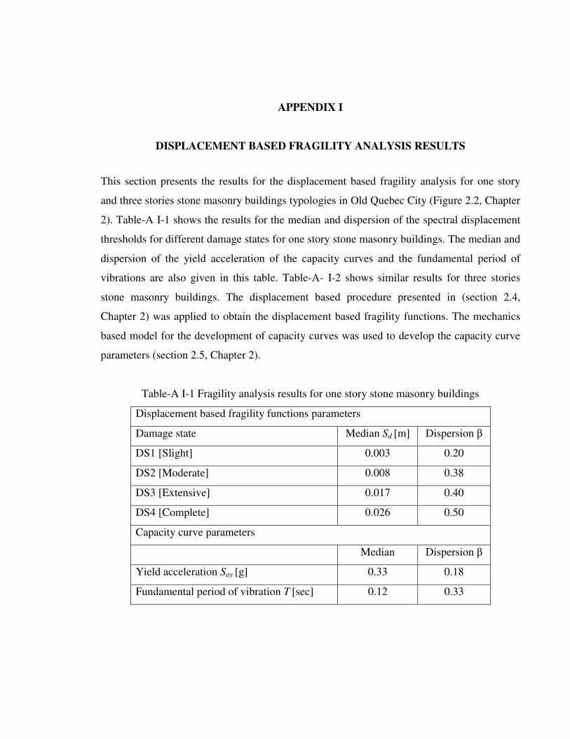
APPENDIX I
DISPLACEMENT BASED FRAGILITY ANALYSIS RESULTS
This section presents the results for the displacement based fragility analysis for one story
and three stories stone masonry buildings typologies in Old Quebec City (Figure 2.2, Chapter
2). Table-A I-1 shows the results for the median and dispersion of the spectral displacement
thresholds for different damage states for one story stone masonry buildings. The median and
dispersion of the yield acceleration of the capacity curves and the fundamental period of
vibrations are also given in this table. Table-A- I-2 shows similar results for three stories
stone masonry buildings. The displacement based procedure presented in (section 2.4,
Chapter 2) was applied to obtain the displacement based fragility functions. The mechanics
based model for the development of capacity curves was used to develop the capacity curve
parameters (section 2.5, Chapter 2).
Table-A I-1 Fragility analysis results for one story stone masonry buildings
Displacement based fragility functions parameters
Damage state Median Sd [m] Dispersion �
DS1 [Slight] 0.003 0.20
DS2 [Moderate] 0.008 0.38
DS3 [Extensive] 0.017 0.40
DS4 [Complete] 0.026 0.50
Capacity curve parameters
Median Dispersion �
Yield acceleration Say [g] 0.33 0.18
Fundamental period of vibration T [sec] 0.12 0.33

112
Table-A I-2 Fragility analysis results for three stories stone masonry buildings
Displacement based fragility functions parameters
Damage state Median Sd [m] Dispersion �
DS1 [Slight] 0.008 0.20
DS2 [Moderate] 0.014 0.38
DS3 [Extensive] 0.025 0.40
DS4 [Complete] 0.033 0.50
Capacity curve parameters
Median Dispersion �
Yield acceleration Say [g] 0.24 0.40
Fundamental period of vibration T [sec] 0.35 0.35
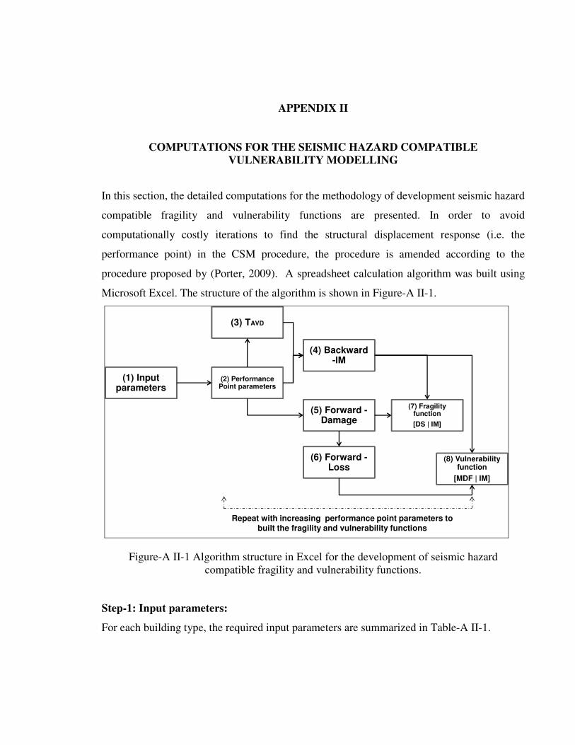
APPENDIX II
COMPUTATIONS FOR THE SEISMIC HAZARD COMPATIBLE VULNERABILITY MODELLING
In this section, the detailed computations for the methodology of development seismic hazard
compatible fragility and vulnerability functions are presented. In order to avoid
computationally costly iterations to find the structural displacement response (i.e. the
performance point) in the CSM procedure, the procedure is amended according to the
procedure proposed by (Porter, 2009). A spreadsheet calculation algorithm was built using
Microsoft Excel. The structure of the algorithm is shown in Figure-A II-1.
(3) TAVD
(4) Backward -IM
(2) Performance Point parameters
(1) Input parameters
(5) Forward -Damage
(6) Forward -Loss
(8) Vulnerability function
[MDF | IM]
Repeat with increasing performance point parameters to built the fragility and vulnerability functions
(7) Fragility function
[DS | IM]
Figure-A II-1 Algorithm structure in Excel for the development of seismic hazard compatible fragility and vulnerability functions.
Step-1: Input parameters:
For each building type, the required input parameters are summarized in Table-A II-1.

114
Table-A II-1 Input parameters
Capacity Curve parameters: Yield Displacement Dy(m)
Yield Acceleration Ay (g)
Ultimate Displacement Du (m)
Ultimate Acceleration Au (g) Elastic damping ratio e Degradation factor �
Displacement Fragility Functions parameters:
Slight damage median � 1 (m) Slight damage log-Standard deviation �1 Moderate damage median � 2 (m) Moderate damage log-Standard deviation �2 Extensive damage median � 3 (m) Extensive damage log-Standard deviation �3 Complete damage median � 4 (m) Complete damage log-Standard deviation �4
Seismic setting parameters: A ground motion prediction equation (GMPE). Site class : A (Hard rock), B(Rock), C(Very Dense
soils), D(Stiff soils), E(Soft soils) Magnitude (M) Distance, R (km)
Step-2: Performance point parameters:
This is the central step of the procedure from which calculations are carried out backward to
evaluate the structure-independent intensity measure IM and forward to damage and loss
analysis. The performance point is defined as the intersection of the capacity curve and the
demand spectrum (over-damped spectrum) with known values of (Sd ,Sa, T, eff ). T denote
the effective period at the performance point. The procedure starts with assuming a value of
Sd, calculate Sa of the performance point from the capacity curve, calculate effective damping
and period which is illustrated in Figure-A II-2.
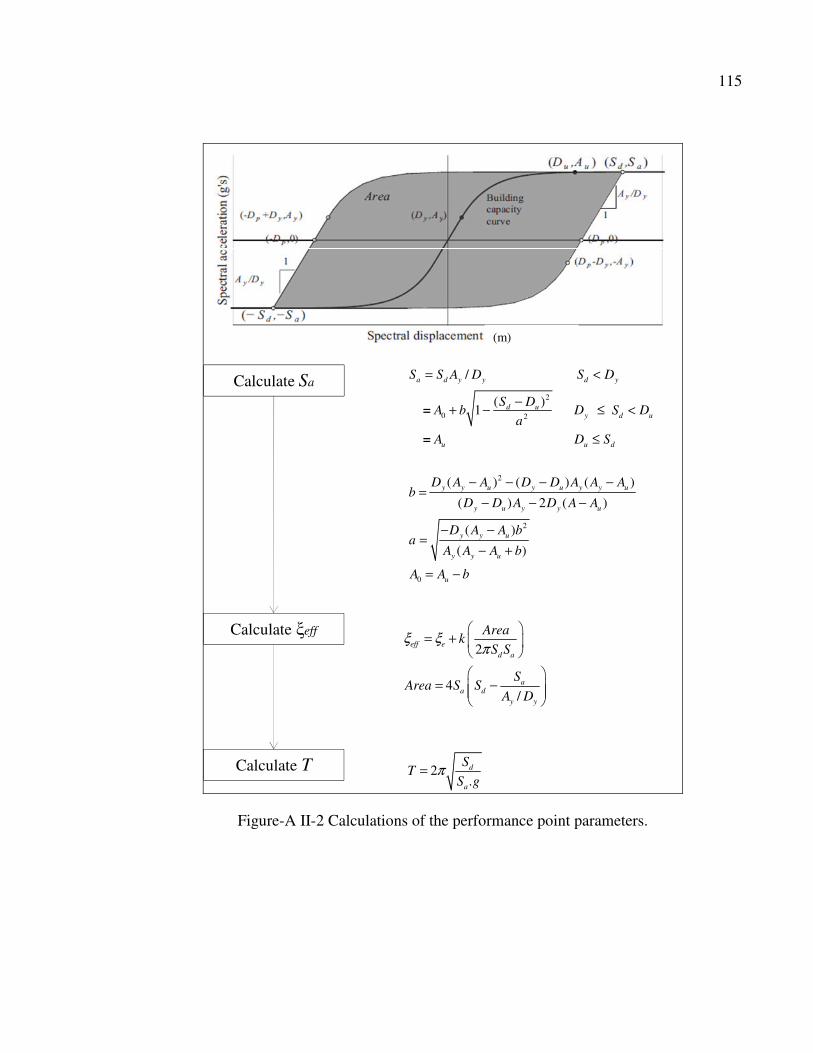
115
(m)
2
0 2
2
2
/
( )1
( ) ( ) ( )
( ) 2 ( )
( )
(
a d y y d y
d uy d u
u u d
y y u y u y y u
y u y y u
y y u
y y u
S S A D S D
S DA b D S D
aA D S
D A A D D A A Ab
D D A D A A
D A A ba
A A A
= <
−+ − ≤ <
≤
− − − −=
− − −
− −=
−
=
=
0
)
u
b
A A b
+
= −
2
4/
eff ed a
aa d
y y
Areak
S S
SArea S S
A D
ξ ξπ
� �= +
� �� �
= − � �
2.d
a
ST
S gπ=
Calculate Sa
Calculate eff
Calculate T
Figure-A II-2 Calculations of the performance point parameters.
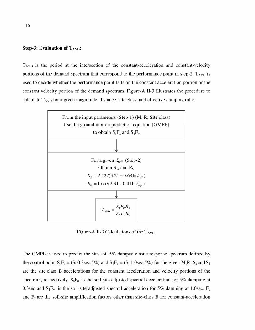
116
Step-3: Evaluation of TAVD:
TAVD is the period at the intersection of the constant-acceleration and constant-velocity
portions of the demand spectrum that correspond to the performance point in step-2. TAVD is
used to decide whether the performance point falls on the constant acceleration portion or the
constant velocity portion of the demand spectrum. Figure-A II-3 illustrates the procedure to
calculate TAVD for a given magnitude, distance, site class, and effective damping ratio.
From the input parameters (Step-1) (M, R, Site class)
Use the ground motion prediction equation (GMPE)
to obtain SsFa and S1Fv
For a given ,eff (Step-2)
Obtain RA and RV
1 V AAVD
S a V
S F RT
S F R=
2.12 /(3.21 0.68ln )
1.65 /(2.31 0.41ln )A eff
V eff
R
R
ξ
ξ
= −
= −
Figure-A II-3 Calculations of the TAVD.
The GMPE is used to predict the site-soil 5% damped elastic response spectrum defined by
the control point SsFa = (Sa0.3sec,5%) and S1Fv = (Sa1.0sec,5%) for the given M,R. Ss and S1
are the site class B accelerations for the constant acceleration and velocity portions of the
spectrum, respectively. SsFa is the soil-site adjusted spectral acceleration for 5% damping at
0.3sec and S1Fv is the soil-site adjusted spectral acceleration for 5% damping at 1.0sec. Fa
and Fv are the soil-site amplification factors other than site-class B for constant-acceleration

117
portion and constant-velocity portion of the spectrum, respectively (Table-A II-2). RA and RV
are the damping reduction factor for damping ratios more than 5% for constant-acceleration
portion and constant-velocity portion of the spectrum, respectively. It should be noted that
the NBCC (2010) applies equivalent amplification factors to the FEMA (2003) with a
reference site class C. The application of the FEMA (2003) site-amplification factors is
adopted in order to be compatible with the values implemented in Hazus where site-class B is
used as the reference site in the GMPE.
Table-A II-2 Site amplification factors (FEMA, 2003).
Site class
A B C D E
Ss (g) Fa
<0.25 0.8 1.0 1.2 1.6 2.5
0.5 0.8 1.0 1.2 1.4 1.7
0.75 0.8 1.0 1.1 1.2 1.2
1.0 0.8 1.0 1.0 1.1 0.9
>1.25 0.8 1.0 1.0 1.0 0.8
S1 (g) Fv
<0.1 0.8 1.0 1.7 2.4 3.5
0.2 0.8 1.0 1.6 2.0 3.2
0.3 0.8 1.0 1.5 1.8 2.8
0.4 0.8 1.0 1.4 1.6 2.4
>0.5 0.8 1.0 1.3 1.5 2.0
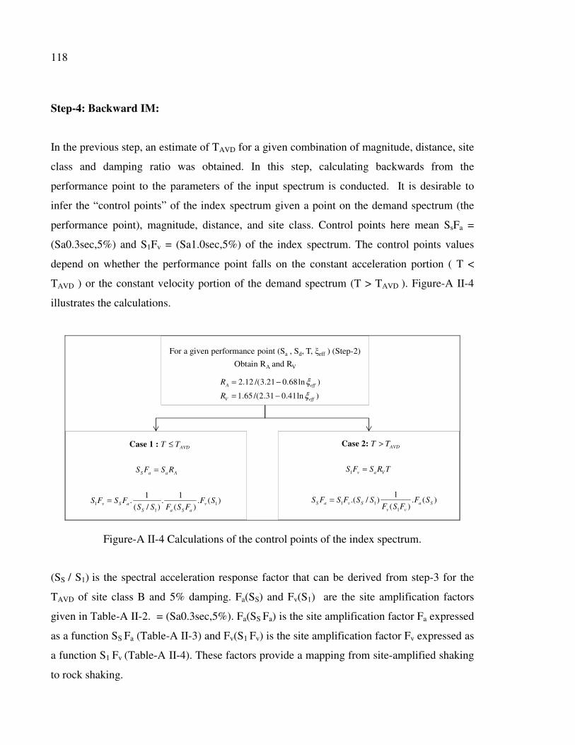
118
Step-4: Backward IM:
In the previous step, an estimate of TAVD for a given combination of magnitude, distance, site
class and damping ratio was obtained. In this step, calculating backwards from the
performance point to the parameters of the input spectrum is conducted. It is desirable to
infer the “control points” of the index spectrum given a point on the demand spectrum (the
performance point), magnitude, distance, and site class. Control points here mean SsFa =
(Sa0.3sec,5%) and S1Fv = (Sa1.0sec,5%) of the index spectrum. The control points values
depend on whether the performance point falls on the constant acceleration portion ( T <
TAVD ) or the constant velocity portion of the demand spectrum (T > TAVD ). Figure-A II-4
illustrates the calculations.
For a given performance point (Sa , Sd, T, eff ) (Step-2)
Obtain RA and RV
1 11
1 1. . . ( )( / ) ( )
AVD
S a a A
v S a vS a S a
T T
S F S R
S F S F F SS S F S F
≤
=
=
Case 1 :
2.12 /(3.21 0.68ln )
1.65 /(2.31 0.41ln )
A eff
V eff
R
R
ξ
ξ
= −
= −
1
1 11
1.( / ) . ( )
( )
AVD
v a V
S a v S a Sv v
T T
S F S R T
S F S F S S F SF S F
>
=
=
Case 2:
Figure-A II-4 Calculations of the control points of the index spectrum.
(SS / S1) is the spectral acceleration response factor that can be derived from step-3 for the
TAVD of site class B and 5% damping. Fa(SS) and Fv(S1) are the site amplification factors
given in Table-A II-2. = (Sa0.3sec,5%). Fa(SS Fa) is the site amplification factor Fa expressed
as a function SS Fa (Table-A II-3) and Fv(S1 Fv) is the site amplification factor Fv expressed as
a function S1 Fv (Table-A II-4). These factors provide a mapping from site-amplified shaking
to rock shaking.
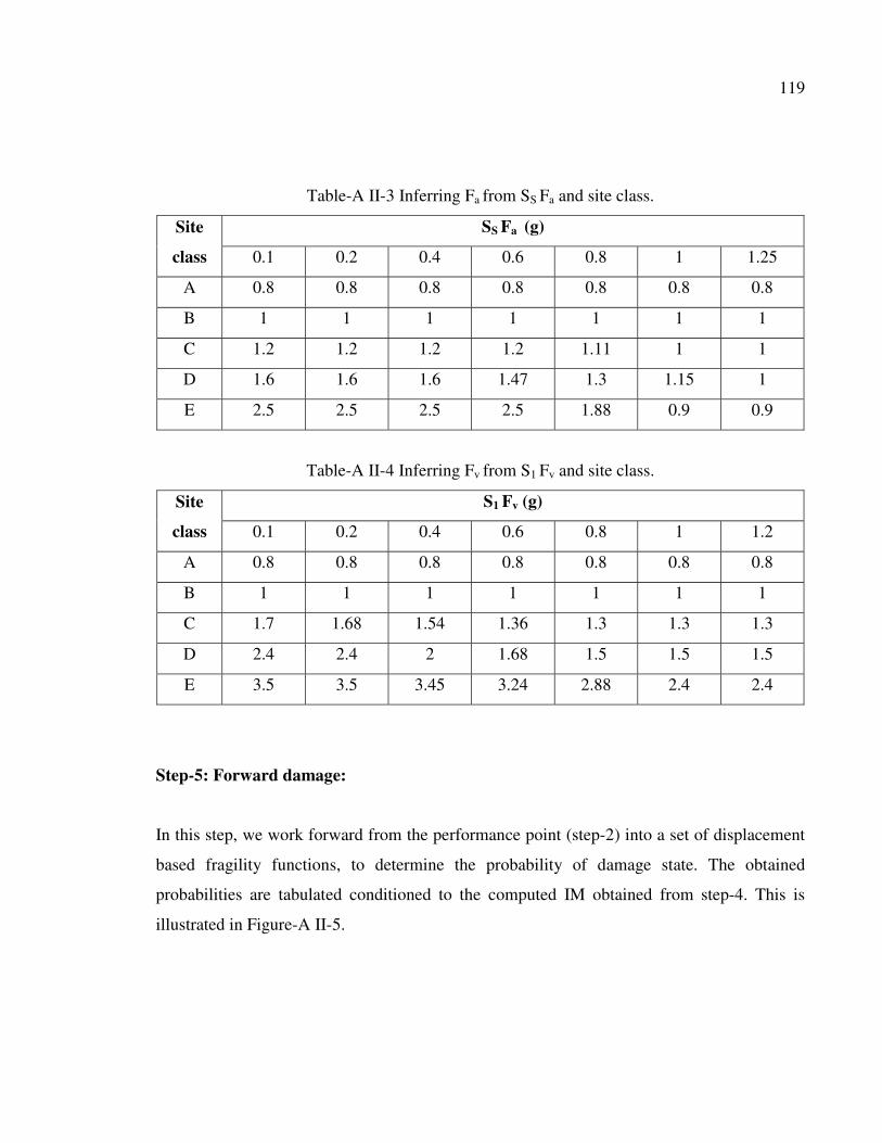
119
Table-A II-3 Inferring Fa from SS Fa and site class.
Site
class
SS Fa (g)
0.1 0.2 0.4 0.6 0.8 1 1.25
A 0.8 0.8 0.8 0.8 0.8 0.8 0.8
B 1 1 1 1 1 1 1
C 1.2 1.2 1.2 1.2 1.11 1 1
D 1.6 1.6 1.6 1.47 1.3 1.15 1
E 2.5 2.5 2.5 2.5 1.88 0.9 0.9
Table-A II-4 Inferring Fv from S1 Fv and site class.
Site
class
S1 Fv (g)
0.1 0.2 0.4 0.6 0.8 1 1.2
A 0.8 0.8 0.8 0.8 0.8 0.8 0.8
B 1 1 1 1 1 1 1
C 1.7 1.68 1.54 1.36 1.3 1.3 1.3
D 2.4 2.4 2 1.68 1.5 1.5 1.5
E 3.5 3.5 3.45 3.24 2.88 2.4 2.4
Step-5: Forward damage:
In this step, we work forward from the performance point (step-2) into a set of displacement
based fragility functions, to determine the probability of damage state. The obtained
probabilities are tabulated conditioned to the computed IM obtained from step-4. This is
illustrated in Figure-A II-5.
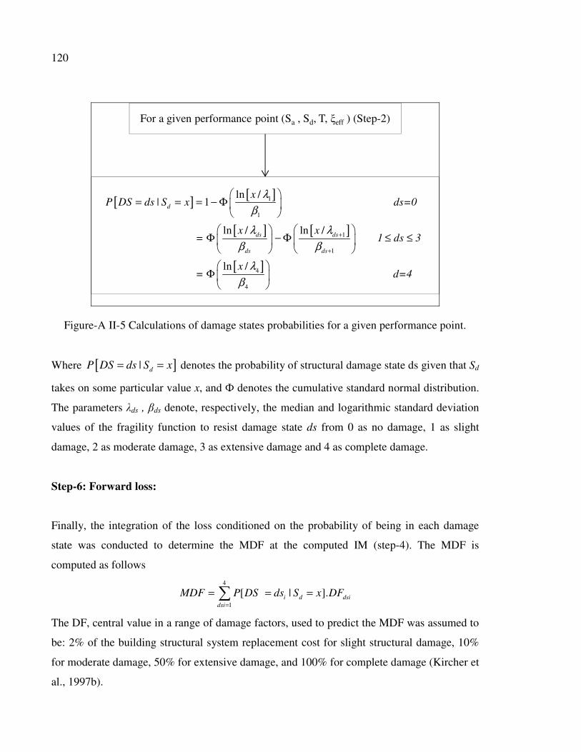
120
For a given performance point (Sa , Sd, T, eff ) (Step-2)
[ ][ ]
[ ] [ ]
[ ]
1
1
1
1
4
ln /| 1
ln / ln /
ln /
d
ds ds
ds ds
xP DS ds S x ds=0
x x = 1 ds 3
x =
λ
β
λ λ
β β
λ
β
+
+
� �= = = − Φ
� �� � � �
Φ − Φ ≤ ≤ � � � �
Φ4
d=4
� � � �
Figure-A II-5 Calculations of damage states probabilities for a given performance point.
Where [ ]| dP DS ds S x= = denotes the probability of structural damage state ds given that Sd
takes on some particular value x, and � denotes the cumulative standard normal distribution.
The parameters �ds , �ds denote, respectively, the median and logarithmic standard deviation
values of the fragility function to resist damage state ds from 0 as no damage, 1 as slight
damage, 2 as moderate damage, 3 as extensive damage and 4 as complete damage.
Step-6: Forward loss:
Finally, the integration of the loss conditioned on the probability of being in each damage
state was conducted to determine the MDF at the computed IM (step-4). The MDF is
computed as follows
4
1
[ | ].i d dsidsi
MDF P DS ds S x DF=
= = =�
The DF, central value in a range of damage factors, used to predict the MDF was assumed to
be: 2% of the building structural system replacement cost for slight structural damage, 10%
for moderate damage, 50% for extensive damage, and 100% for complete damage (Kircher et
al., 1997b).

121
Step-7 and 8: Hazard compatible fragility and vulnerability functions:
To establish the fragility and vulnerability functions in terms of structure-independent IMs,
the procedure is repeated for increasing values of the performance points (step-2). The
computed probabilistic damage states and mean damage factor are given in tabular format for
respective structure-independent IM. The data are then fitted to provide suitable hazard
compatible seismic fragility (Figure-A II-6) and vulnerability functions (Figure-A II-7) as a
lognormal cumulative distribution functions.
0.0
0.2
0.4
0.6
0.8
1.0
0.00 0.50 1.00 1.50 2.00 2.50
P [
DS
]
Ss Fa = Sa(0.3sec,5%) [g]
DS1DS2DS3DS4Prob(DS1)Prob(DS2)Prob(DS3)Prob(DS4)
Figure-A II-6 Illustration of the fitted lognormal distribution for the hazard compatible fragility functions.

122
0.0
0.2
0.4
0.6
0.8
1.0
0.00 0.50 1.00 1.50 2.00 2.50
MD
F
Ss Fa = Sa(0.3sec,5%) [g]
Figure-A II-7 Illustration of the fitted lognormal distribution for the hazard compatible vulnerability functions.
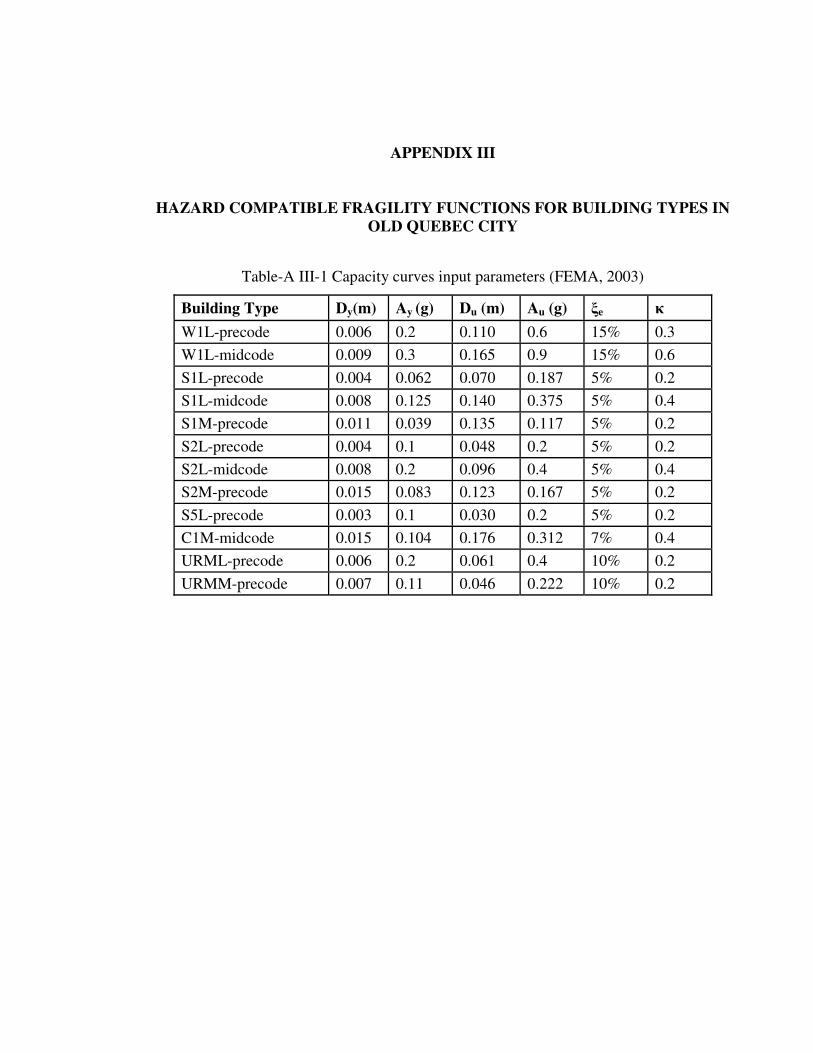
APPENDIX III
HAZARD COMPATIBLE FRAGILITY FUNCTIONS FOR BUILDING TYPES IN OLD QUEBEC CITY
Table-A III-1 Capacity curves input parameters (FEMA, 2003)
Building Type Dy(m) Ay (g) Du (m) Au (g) �e �
W1L-precode 0.006 0.2 0.110 0.6 15% 0.3
W1L-midcode 0.009 0.3 0.165 0.9 15% 0.6
S1L-precode 0.004 0.062 0.070 0.187 5% 0.2
S1L-midcode 0.008 0.125 0.140 0.375 5% 0.4
S1M-precode 0.011 0.039 0.135 0.117 5% 0.2
S2L-precode 0.004 0.1 0.048 0.2 5% 0.2
S2L-midcode 0.008 0.2 0.096 0.4 5% 0.4
S2M-precode 0.015 0.083 0.123 0.167 5% 0.2
S5L-precode 0.003 0.1 0.030 0.2 5% 0.2
C1M-midcode 0.015 0.104 0.176 0.312 7% 0.4
URML-precode 0.006 0.2 0.061 0.4 10% 0.2
URMM-precode 0.007 0.11 0.046 0.222 10% 0.2
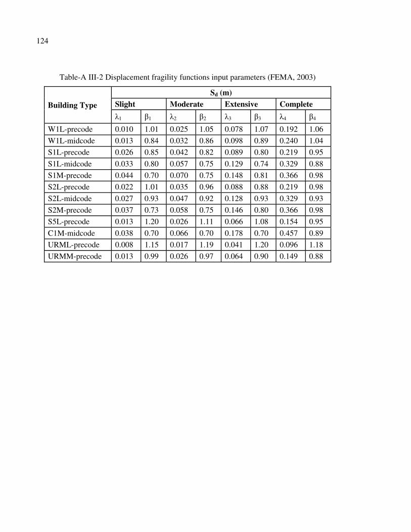
124
Table-A III-2 Displacement fragility functions input parameters (FEMA, 2003)
Building Type
Sd (m) Slight Moderate Extensive Complete
�1 �1 �2 �2 �3 �3 �4 �4
W1L-precode 0.010 1.01 0.025 1.05 0.078 1.07 0.192 1.06
W1L-midcode 0.013 0.84 0.032 0.86 0.098 0.89 0.240 1.04
S1L-precode 0.026 0.85 0.042 0.82 0.089 0.80 0.219 0.95
S1L-midcode 0.033 0.80 0.057 0.75 0.129 0.74 0.329 0.88
S1M-precode 0.044 0.70 0.070 0.75 0.148 0.81 0.366 0.98
S2L-precode 0.022 1.01 0.035 0.96 0.088 0.88 0.219 0.98
S2L-midcode 0.027 0.93 0.047 0.92 0.128 0.93 0.329 0.93
S2M-precode 0.037 0.73 0.058 0.75 0.146 0.80 0.366 0.98
S5L-precode 0.013 1.20 0.026 1.11 0.066 1.08 0.154 0.95
C1M-midcode 0.038 0.70 0.066 0.70 0.178 0.70 0.457 0.89
URML-precode 0.008 1.15 0.017 1.19 0.041 1.20 0.096 1.18
URMM-precode 0.013 0.99 0.026 0.97 0.064 0.90 0.149 0.88
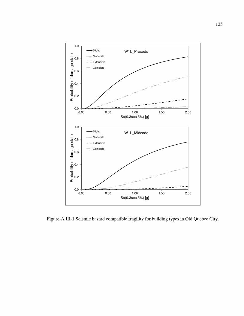
125
0.0
0.2
0.4
0.6
0.8
1.0
0.00 0.50 1.00 1.50 2.00
Pro
babi
lity
of d
amag
e st
ate
Sa(0.3sec,5%) [g]
W1L_PrecodeSlight
Moderate
Extensitve
Complete
0.0
0.2
0.4
0.6
0.8
1.0
0.00 0.50 1.00 1.50 2.00
Pro
babi
lity
of d
amag
e st
ate
Sa(0.3sec,5%) [g]
W1L_MidcodeSlight
Moderate
Extensitve
Complete
Figure-A III-1 Seismic hazard compatible fragility for building types in Old Quebec City.
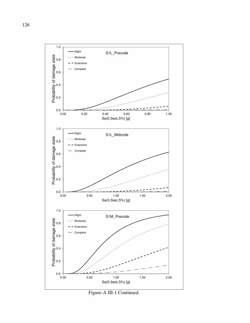
126
0.0
0.2
0.4
0.6
0.8
1.0
0.00 0.20 0.40 0.60 0.80 1.00
Pro
babi
lity
of d
amag
e st
ate
Sa(0.3sec,5%) [g]
S1L_PrecodeSlight
Moderate
Extensitve
Complete
0.0
0.2
0.4
0.6
0.8
1.0
0.00 0.50 1.00 1.50 2.00
Pro
babi
lity
of d
amag
e st
ate
Sa(0.3sec,5%) [g]
S1L_MidcodeSlight
Moderate
Extensitve
Complete
0.0
0.2
0.4
0.6
0.8
1.0
0.00 0.50 1.00 1.50 2.00
Pro
babi
lity
of d
amag
e st
ate
Sa(0.3sec,5%) [g]
S1M_PrecodeSlight
Moderate
Extensitve
Complete
Figure-A III-1 Continued.
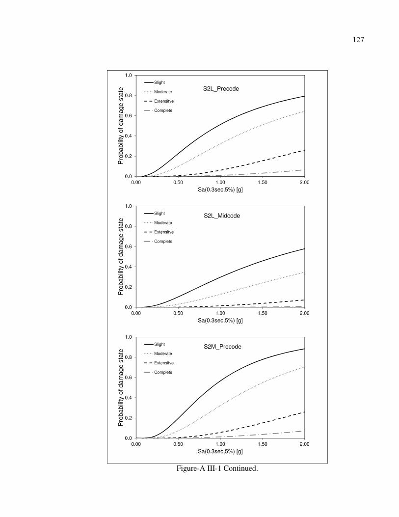
127
0.0
0.2
0.4
0.6
0.8
1.0
0.00 0.50 1.00 1.50 2.00
Pro
babi
lity
of d
amag
e st
ate
Sa(0.3sec,5%) [g]
S2L_PrecodeSlight
Moderate
Extensitve
Complete
0.0
0.2
0.4
0.6
0.8
1.0
0.00 0.50 1.00 1.50 2.00
Pro
babi
lity
of d
amag
e st
ate
Sa(0.3sec,5%) [g]
S2L_MidcodeSlight
Moderate
Extensitve
Complete
0.0
0.2
0.4
0.6
0.8
1.0
0.00 0.50 1.00 1.50 2.00
Pro
babi
lity
of d
amag
e st
ate
Sa(0.3sec,5%) [g]
S2M_PrecodeSlight
Moderate
Extensitve
Complete
Figure-A III-1 Continued.

128
0.0
0.2
0.4
0.6
0.8
1.0
0.00 0.50 1.00 1.50 2.00
Pro
babi
lity
of d
amag
e st
ate
Sa(0.3sec,5%) [g]
S5L_PrecodeSlight
Moderate
Extensitve
Complete
0.0
0.2
0.4
0.6
0.8
1.0
0.00 0.50 1.00 1.50 2.00
Pro
babi
lity
of d
amag
e st
ate
Sa(0.3sec,5%) [g]
C1M_MidcodeSlight
Moderate
Extensitve
Complete
0.0
0.2
0.4
0.6
0.8
1.0
0.00 0.50 1.00 1.50 2.00
Pro
babi
lity
of d
amag
e st
ate
Sa(0.3sec,5%) [g]
URMBL_PrecodeSlight
Moderate
Extensitve
Complete
Figure-A III-1 Continued.
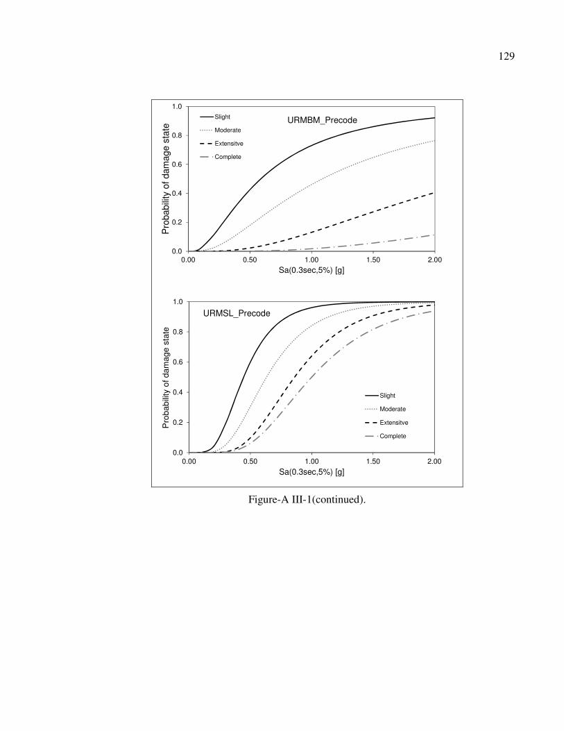
129
0.0
0.2
0.4
0.6
0.8
1.0
0.00 0.50 1.00 1.50 2.00
Pro
babi
lity
of d
amag
e st
ate
Sa(0.3sec,5%) [g]
URMBM_PrecodeSlight
Moderate
Extensitve
Complete
0.0
0.2
0.4
0.6
0.8
1.0
0.00 0.50 1.00 1.50 2.00
Pro
babi
lity
of d
amag
e st
ate
Sa(0.3sec,5%) [g]
URMSL_Precode
Slight
Moderate
Extensitve
Complete
Figure-A III-1(continued).


APPENDIX IV
ATKINSON AND BOORE (2006) GROUND MOTION PREDICTION EQUATION FOR EASTREN NORTH AMERICA
Atkinson and Boore (2006) ground motion prediction equation to estimate the spectral
acceleration at a particular period for a Magnitude (M) at distance from fault rupture (R)
takes the following form:
21 2 3 4 5 1 6 7 2 8 9 0 10[ ( )] ( ) ( ) ( )aLog S T c c M c M c c M f c c M f c c M f c R S= + + + + + + + + ++
Where: f0 = max (log (R0/R), 0); f1 = min (log R, log R1); f2 = max (log (R/R2), 0); R0 =10; R1 = 70;
R2 = 140 and S is the soil site parameter that takes the form:
{ }{ }
230
230
log exp ln( / ) ln(60 /100) for pgaBC 60cm/s
log exp ln( / ) ( /100) for pgaBC > 60cm/s
lin ref nl
lin ref nl
S b V V b
S b V V b pgaBC
� �= + ≤ �
� �= + �
1 30 1
1 2 30 2 1 2 2 1 30 2
2 30 2 2 30
for V
( - )ln(V / ) / ln( / ) for V
ln(V /V ) / ln( / ) for V
nl
nl
nl ref ref ref
nl
b b
b b b b
b b V V
b
υ
υ υ υ υ υ
υ υ
= ≤
= + < <
= < <
300.0 for V refV= >
Where :
V30 is the soil shear-wave velocity in the upper 30m; pgaBC is the predicted value of PGA
for V30 = 760m/sec; and Vref = 760 m/sec (limit between site-class B and C), 2 = 300 m/sec
(limit for site-class D) and 1 = 180 m/sec (limit for site-class E).
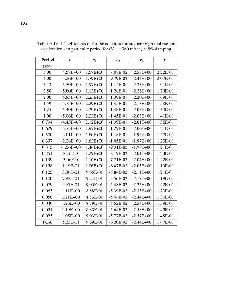
132
Table-A IV-1 Coefficients of for the equation for predicting ground motion acceleration at a particular period for (V30 = 760 m/sec) at 5% damping.
Period c1 c2 c3 c4 c5
(sec) 5.00 -4.58E+00 1.58E+00 -8.07E-02 -2.53E+00 2.22E-01 4.00 -5.26E+00 1.79E+00 -9.79E-02 -2.44E+00 2.07E-01 3.13 -5.59E+00 1.97E+00 -1.14E-01 -2.33E+00 1.91E-01 2.50 -5.80E+00 2.13E+00 -1.28E-01 -2.26E+00 1.79E-01 2.00 -5.85E+00 2.23E+00 -1.39E-01 -2.20E+00 1.69E-01 1.59 -5.75E+00 2.29E+00 -1.45E-01 -2.13E+00 1.58E-01 1.25 -5.49E+00 2.29E+00 -1.48E-01 -2.08E+00 1.50E-01 1.00 -5.06E+00 2.23E+00 -1.45E-01 -2.03E+00 1.41E-01
0.794 -4.45E+00 2.12E+00 -1.39E-01 -2.01E+00 1.36E-01 0.629 -3.75E+00 1.97E+00 -1.29E-01 -2.00E+00 1.31E-01 0.500 -3.01E+00 1.80E+00 -1.18E-01 -1.98E+00 1.27E-01 0.397 -2.28E+00 1.63E+00 -1.05E-01 -1.97E+00 1.23E-01 0.315 -1.56E+00 1.46E+00 -9.31E-02 -1.98E+00 1.21E-01 0.251 -8.76E-01 1.29E+00 -8.19E-02 -2.01E+00 1.23E-01 0.199 -3.06E-01 1.16E+00 -7.21E-02 -2.04E+00 1.22E-01 0.158 1.19E-01 1.06E+00 -6.47E-02 -2.05E+00 1.19E-01 0.125 5.36E-01 9.65E-01 -5.84E-02 -2.11E+00 1.21E-01 0.100 7.82E-01 9.24E-01 -5.56E-02 -2.17E+00 1.19E-01 0.079 9.67E-01 9.03E-01 -5.48E-02 -2.25E+00 1.22E-01 0.063 1.11E+00 8.88E-01 -5.39E-02 -2.33E+00 1.23E-01 0.050 1.21E+00 8.83E-01 -5.44E-02 -2.44E+00 1.30E-01 0.040 1.26E+00 8.79E-01 -5.52E-02 -2.54E+00 1.39E-01 0.031 1.19E+00 8.88E-01 -5.64E-02 -2.58E+00 1.45E-01 0.025 1.05E+00 9.03E-01 -5.77E-02 -2.57E+00 1.48E-01 PGA 5.23E-01 9.69E-01 -6.20E-02 -2.44E+00 1.47E-01
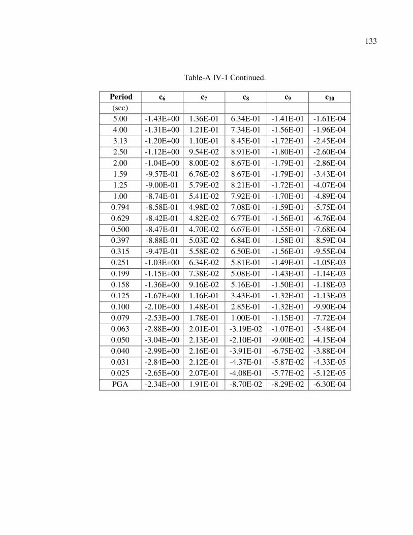
133
Table-A IV-1 Continued.
Period c6 c7 c8 c9 c10 (sec) 5.00 -1.43E+00 1.36E-01 6.34E-01 -1.41E-01 -1.61E-04 4.00 -1.31E+00 1.21E-01 7.34E-01 -1.56E-01 -1.96E-04 3.13 -1.20E+00 1.10E-01 8.45E-01 -1.72E-01 -2.45E-04 2.50 -1.12E+00 9.54E-02 8.91E-01 -1.80E-01 -2.60E-04 2.00 -1.04E+00 8.00E-02 8.67E-01 -1.79E-01 -2.86E-04 1.59 -9.57E-01 6.76E-02 8.67E-01 -1.79E-01 -3.43E-04 1.25 -9.00E-01 5.79E-02 8.21E-01 -1.72E-01 -4.07E-04 1.00 -8.74E-01 5.41E-02 7.92E-01 -1.70E-01 -4.89E-04
0.794 -8.58E-01 4.98E-02 7.08E-01 -1.59E-01 -5.75E-04 0.629 -8.42E-01 4.82E-02 6.77E-01 -1.56E-01 -6.76E-04 0.500 -8.47E-01 4.70E-02 6.67E-01 -1.55E-01 -7.68E-04 0.397 -8.88E-01 5.03E-02 6.84E-01 -1.58E-01 -8.59E-04 0.315 -9.47E-01 5.58E-02 6.50E-01 -1.56E-01 -9.55E-04 0.251 -1.03E+00 6.34E-02 5.81E-01 -1.49E-01 -1.05E-03 0.199 -1.15E+00 7.38E-02 5.08E-01 -1.43E-01 -1.14E-03 0.158 -1.36E+00 9.16E-02 5.16E-01 -1.50E-01 -1.18E-03 0.125 -1.67E+00 1.16E-01 3.43E-01 -1.32E-01 -1.13E-03 0.100 -2.10E+00 1.48E-01 2.85E-01 -1.32E-01 -9.90E-04 0.079 -2.53E+00 1.78E-01 1.00E-01 -1.15E-01 -7.72E-04 0.063 -2.88E+00 2.01E-01 -3.19E-02 -1.07E-01 -5.48E-04 0.050 -3.04E+00 2.13E-01 -2.10E-01 -9.00E-02 -4.15E-04 0.040 -2.99E+00 2.16E-01 -3.91E-01 -6.75E-02 -3.88E-04 0.031 -2.84E+00 2.12E-01 -4.37E-01 -5.87E-02 -4.33E-05 0.025 -2.65E+00 2.07E-01 -4.08E-01 -5.77E-02 -5.12E-05 PGA -2.34E+00 1.91E-01 -8.70E-02 -8.29E-02 -6.30E-04

134
Table-A IV-2 Coefficients of site response.
Period blin b1 b2
(sec) 5.00 -0.752 -0.300 0.000 4.00 -0.745 -0.310 0.000 3.13 -0.740 -0.330 0.000 2.50 -0.735 -0.357 0.000 2.00 -0.730 -0.375 0.000 1.59 -0.726 -0.395 0.000 1.25 -0.738 -0.420 0.000 1.00 -0.700 -0.440 0.000
0.794 -0.690 -0.465 -0.002 0.629 -0.670 -0.480 -0.031 0.500 -0.600 -0.495 -0.060 0.397 -0.500 -0.508 -0.095 0.315 -0.445 -0.513 -0.130 0.251 -0.390 -0.518 -0.160 0.199 -0.306 -0.521 -0.185 0.158 -0.280 -0.528 -0.185 0.125 -0.260 -0.560 -0.140 0.100 -0.250 -0.595 -0.132 0.079 -0.232 -0.637 -0.117 0.063 -0.249 -0.642 -0.105 0.050 -0.286 -0.643 -0.105 0.040 -0.314 -0.609 -0.105 0.031 -0.322 -0.618 -0.108 0.025 -0.330 -0.624 -0.115 PGA -0.361 -0.641 -0.144

APPENDIX V
COMPARISON WITH HAZUS SOFTWARE
The procedure presented in APPENDIX-I showed similar results when compared to the
procedure implemented in HAZUS software tool for a ground motion input of
Sa(0.3s)=0.38g and Sa(1.0s)=0.07g. The comparison of probability of structural damage is
conducted for four building classes: URML_Precode, S2L_Precode, W1L_Precode and
S1L_Precode. The results are summarized in Table-A V-1. Figures A-V-1 to A-V-8 presents
the damage prediction using the fragility functions developed using the procedure proposed
in this study and the results from HAZUS software.
Table-A V-1 Comparison of probability of damage with HAZUS software.
URMBL_Precode S2L_Precode W1L_Precode S1L_Precode
Probability [%]
Fragility functions
HAZUS software
Fragility functions
HAZUS software
Fragility functions
HAZUS software
Fragility functions
HAZUS software
None 64 66 86 87 79 79 89 84
Slight 19 18 9 9 16 16 8 13
Moderate 13 12 5 5 5 4 3 3
Extensive 4 3 0 0 0 0 0 0
Complete 1 1 0 0 0 0 0 0
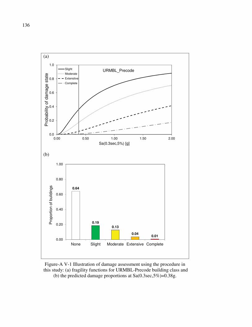
136
(a)
0.0
0.2
0.4
0.6
0.8
1.0
0.00 0.50 1.00 1.50 2.00
Pro
babi
lity
of d
amag
e st
ate
Sa(0.3sec,5%) [g]
URMBL_PrecodeSlight
Moderate
Extensitve
Complete
(b)
0.64
0.190.13
0.040.01
0.00
0.20
0.40
0.60
0.80
1.00
None Slight Moderate Extensive Complete
Pro
port
ion
of b
uild
ings
Figure-A V-1 Illustration of damage assessment using the procedure in this study: (a) fragility functions for URMBL-Precode building class and
(b) the predicted damage proportions at Sa(0.3sec,5%)=0.38g.

137
Figure-A V-2 HAZUS software damage prediction at Sa(0.3sec,5%)=0.38g for the URML_Precode building class.
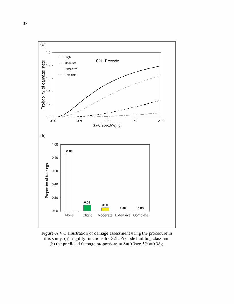
138
(a)
0.0
0.2
0.4
0.6
0.8
1.0
0.00 0.50 1.00 1.50 2.00
Pro
babi
lity
of d
amag
e st
ate
Sa(0.3sec,5%) [g]
S2L_PrecodeSlight
Moderate
Extensitve
Complete
(b)
0.86
0.090.05
0.00 0.000.00
0.20
0.40
0.60
0.80
1.00
None Slight Moderate Extensive Complete
Pro
port
ion
of b
uild
ings
Figure-A V-3 Illustration of damage assessment using the procedure in this study: (a) fragility functions for S2L-Precode building class and
(b) the predicted damage proportions at Sa(0.3sec,5%)=0.38g.
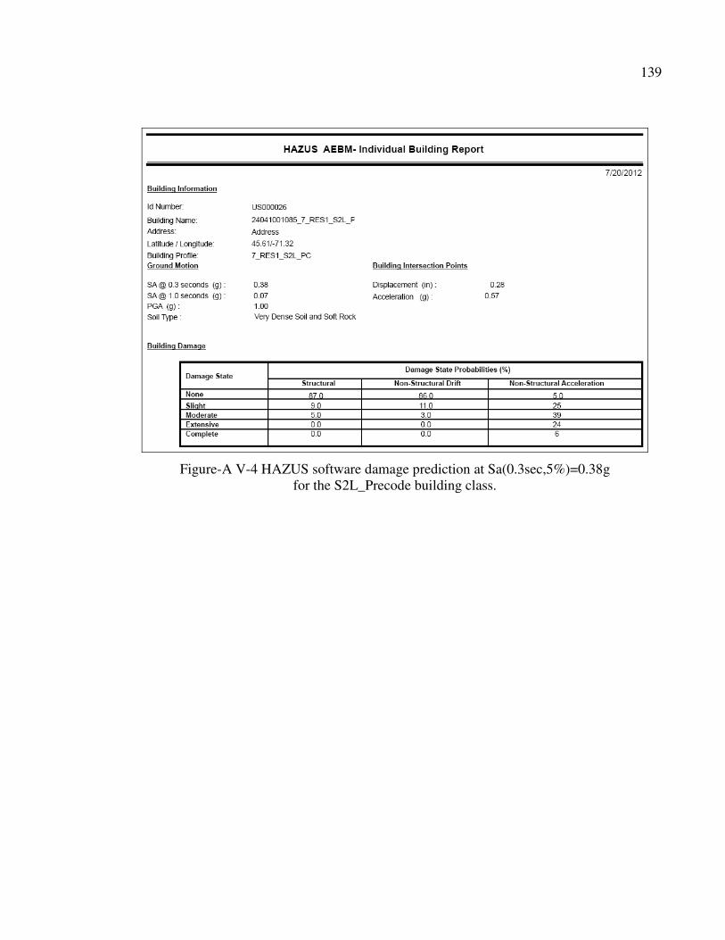
139
Figure-A V-4 HAZUS software damage prediction at Sa(0.3sec,5%)=0.38g for the S2L_Precode building class.

140
(a)
0.0
0.2
0.4
0.6
0.8
1.0
0.00 0.50 1.00 1.50 2.00
Pro
babi
lity
of d
amag
e st
ate
Sa(0.3sec,5%) [g]
W1L_PrecodeSlight
Moderate
Extensitve
Complete
(b)
0.79
0.16
0.050.00 0.00
0.00
0.20
0.40
0.60
0.80
1.00
None Slight Moderate Extensive Complete
Pro
port
ion
of b
uild
ings
Figure-A V-5 Illustration of damage assessment using the procedure in this study: (a) fragility functions for W1L-Precode building class and
(b) the predicted damage proportions at Sa(0.3sec,5%)=0.38g.

141
Figure-A V-6 HAZUS software damage prediction at Sa(0.3sec,5%)=0.38g for the W1L_Precode building class.
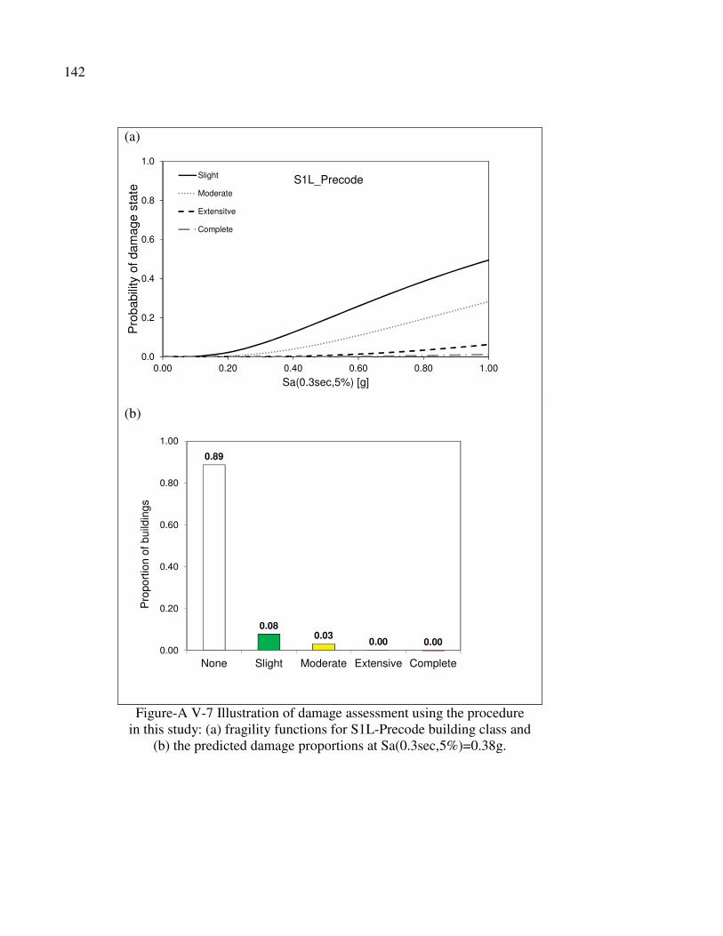
142
(a)
0.0
0.2
0.4
0.6
0.8
1.0
0.00 0.20 0.40 0.60 0.80 1.00
Pro
babi
lity
of d
amag
e st
ate
Sa(0.3sec,5%) [g]
S1L_PrecodeSlight
Moderate
Extensitve
Complete
(b)
0.89
0.080.03
0.00 0.000.00
0.20
0.40
0.60
0.80
1.00
None Slight Moderate Extensive Complete
Pro
port
ion
of b
uild
ings
Figure-A V-7 Illustration of damage assessment using the procedure in this study: (a) fragility functions for S1L-Precode building class and
(b) the predicted damage proportions at Sa(0.3sec,5%)=0.38g.
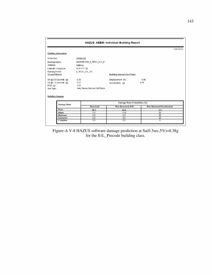
143
Figure-A V-8 HAZUS software damage prediction at Sa(0.3sec,5%)=0.38g for the S1L_Precode building class.


LIST OF BIBLIOGRAPHICAL REFERENCES
Abo-El-Ezz A., M.J. Nollet and M. Nastev. 2011a. « Analytical displacement-based seismic fragility analysis of stone masonry buildings». Proceedings of the 3rd International Conference on Computational Methods in Structural Dynamics and Earthquake Engineering, Corfu, Greece., Paper No.679.
Abo-El-Ezz A., M.J. Nollet and M. Nastev. 2011b. « Characterization of historic stone masonry buildings for seismic risk assessment: a case study at Old Quebec City ». Proceedings of the Canadian Society of Civil Engineering General Conference, Ottawa, Canada. Paper No. GC-223.
Abo-El-Ezz A., M.J. Nollet and M. Nastev. 2012a. « Development of seismic hazard compatible vulnerability functions for stone masonry buildings». Proceedings of the Canadian Society of Civil Engineering 3rd Structural Specialty Conference, Edmonton, Canada., Paper No. STR-1030.
Abo-El-Ezz A., M.J. Nollet and M. Nastev. 2012b. « Regional seismic risk assessment of existing building at Old Quebec City, Canada ». Proceedings of the 15th World Conference on Earthquake Engineering, Lisbon, Portugal, Paper No. 1543.
Abo-El-Ezz A., M.J. Nollet and M. Nastev. 2013a. « Seismic fragility assessment of low-rise stone masonry buildings ». Journal of Earthquake Engineering and Engineering Vibrations,Vol.12 No.1, 2013
Abo-El-Ezz A., M.J. Nollet and M. Nastev. 2013b. « A methodology for rapid earthquake damage assessment of existing buildings ». Accepted for publication in the proceedings of the 3rd Specialty Conference on Disaster Prevention and Mitigation, CSCE, Montreal, Paper. No. DIS-16.
Adams, J., and S. Halchuk. 2003. Fourth generation seismic hazard maps of Canada: Values for over 650 Canadian localities intended for the 2005 National Building Code of Canada. Geological Survey of Canada Open File, vol. 4459, p. 1-155.
Akkar, S., H. Sucuo lu and A. Yakut. 2005. « Displacement-based fragility functions for low-and mid-rise ordinary concrete buildings ». Earthquake Spectra, vol. 21, p. 901.
ASCE. 2007. Seismic rehabilitation of existing building. ASCE Standard no. ASCE/SEI 41-06, American Society of Civil Engineers, USA.
ATC. 1996. ATC-20, Procedures for Post-earthquake Safety Evaluation of Buildings. Applied Technology Council, Redwood City, CA, USA.
146
ATC. 1996. ATC-40, Seismic evaluation and retrofit of concrete buildings, Vol. 1, Applied Technology Council, Redwood City, CA, USA.
Atkinson, G. M., and D. M. Boore. 2006. « Earthquake ground-motion prediction equations for eastern North America ». Bulletin of the Seismological Society of America, vol. 96, no 6, p. 2181-205.
Barron-Corverra R. 2000. « Spectral Evaluation of Seismic Fragility in Structures » PhD Thesis, University at Buffalo, The State University of New York, Buffalo, USA.
Benedetti, D., P. Carydis and P. Pezzoli. 1998. « Shaking table tests on 24 simple masonry buildings ». Earthquake engineering & structural dynamics, vol. 27, no 1, p. 67-90.
Borzi, B., H. Crowley and R. Pinho. 2008. « Simplified pushover-based earthquake loss assessment (SP-BELA) method for masonry buildings ». International Journal of Architectural Heritage, vol. 2, no 4, p. 353-376.
Bosiljkov, V., AW Page, V. Bokan�Bosiljkov and R. Žarni�. 2010. « Evaluation of the seismic performance of brick masonry walls ». Structural Control and Health Monitoring, vol. 17, no 1, p. 100-118.
Bruneau, M. 1994. « State-of-the-art report on seismic performance of unreinforced masonry buildings ». Journal of Structural Engineering, vol. 120, no 1, p. 230-251.
Calderini, C., S. Cattari and S. Lagomarsino. 2009. « In�plane strength of unreinforced masonry piers ». Earthquake engineering & structural dynamics, vol. 38, no 2, p. 243-267.
Calvi, G.M. 1999. « A displacement-based approach for vulnerability evaluation of classes of buildings ». Journal of Earthquake Engineering, vol. 3, no 3, p. 411-438.
Chidiac, SE, S. Foo and MS Cheung. 2000. « Seismic guidelines for stone-masonry components and structures ». In International Conference on Seismic Performance of Traditional Buildings. (Turkey), p. 13.
Chopra, A.K., and R.K. Goel. 1999. « Capacity-demand-diagram methods based on inelastic design spectrum ». Earthquake Spectra, vol. 15, no 4, p. 637-656.
Choun, Y.S., and A.S. Elnashai. 2010. « A simplified framework for probabilistic earthquake loss estimation ». Probabilistic Engineering Mechanics, vol. 25, no 4, p. 355-364.
Coburn, A. and R. Spence. 2002. Earthquake Protection, 2nd Chichester: John Wiley and Sons.
Crowley, H., J. Bommer, J. Pinho and J. Bird. 2005. « The impact of epistemic uncertainty on an earthquake loss model ». Earthquake Engineering and Structural Dynamics, vol. 34, p. 1653–1685.

147
Crowley, H., R. Pinho and J.J. Bommer. 2004. « A probabilistic displacement-based vulnerability assessment procedure for earthquake loss estimation ». Bulletin of Earthquake Engineering, vol. 2, no 2, p. 173-219.
Elmenshawi, A.E.A., M.S.M. Sorour, A.M.A. Mufti, L.G.J.L.G. Jaeger and N.S.N. Shrive. 2010. « In-plane seismic behaviour of historic stone masonry ». Canadian Journal of Civil Engineering, vol. 37, no 3, p. 465-476.
Erberik, M.A. 2008. « Generation of fragility curves for Turkish masonry buildings considering in�plane failure modes ». Earthquake engineering & structural dynamics, vol. 37, no 3, p. 387-405.
Erberik, M.A., and A.S. Elnashai. 2004. « Fragility analysis of flat-slab structures ». Engineering Structures, vol. 26, no 7, p. 937-948.
Erdik, M., K. Sesetyan, M. Demircioglu, U. Hancilar, C. Zulfikar, E. Cakti, Y. Kamer, C. Yenidogan, C. Tuzun and Z. Cagnan. 2010. « Rapid earthquake hazard and loss assessment for Euro-Mediterranean region ». Acta Geophysica, vol. 58, p. 855-892
Fajfar, P. 1999. « Capacity spectrum method based on inelastic demand spectra ». Earthquake Engineering and Structural Dynamics, vol. 28, no 9, p. 979-994.
Fajfar, P. 2000. « A nonlinear analysis method for performance-based seismic design ». Earthquake Spectra, vol. 16, no 3, p. 573-592.
FEMA. 2000. FEMA 356 Prestandard and Commentary for the Seismic Rehabilitation of Buildings. United States Federal Emergency Management Agency, Washington, D.C., USA.
FEMA. 2003. HAZUS-MH MR4: Multi-hazard Loss Estimation Methodology Earthquake Model Technical manual. Federal Emergency Management Agency, National Institute of Building Science, Washington, D.C, USA.
FEMA. 2005. Improvement of nonlinear static seismic analysis procedures, Report Number 440. Federal Emergency Management Agency, Applied Technology Council, Washington D.C., USA.
Frankie T. 2010. « Simulation-based fragility relationships for unreinforced masonry buildings ». Master Thesis, University of Illinois at Urbana Champaign, USA.
Gencturk, Bora, Amr S. Elnashai and Junho Song. 2008. « Fragility Relationships for Populations of Woodframe Structures Based on Inelastic Response ». Journal of Earthquake Engineering, vol. 12, no sup2, p. 119-128.
Giovinazzi S. 2005. «The vulnerability assessment and the damage scenario in seismic risk analysis». PhD Thesis, University of Florence, Italy and Technical University of Braunschweig, Germany.
148
Goel, R.K. 2011. « Variability and accuracy of target displacement from nonlinear static procedures ». International Scholarly Research Network Civil Engineering, Article ID 582426, vol. 2011.
Ingham, J., and M. Griffith. 2011. « Performance of unreinforced masonry buildings during the 2010 Darfield (Christchurch, NZ) earthquake ». Australian Journal of Structural Engineering, vol. 11, no 3, p. 207.
Jeong, S.H., and A.S. Elnashai. 2007. « Probabilistic fragility analysis parameterized by fundamental response quantities ». Engineering Structures, vol. 29, no 6, p. 1238-1251.
Kircher, C.A., A.A. Nassar, O. Kustu and W.T. Holmes. 1997a. « Development of building damage functions for earthquake loss estimation ». Earthquake Spectra, vol. 13, no 4, p. 663-682.
Kircher, C.A., R.K. Reitherman, R.V. Whitman and C. Arnold. 1997b. « Estimation of earthquake losses to buildings ». Earthquake Spectra, vol. 13, no 4, p. 703-720.
Lang, K. 2002. «Seismic Vulnerability of Existing Buildings», Institute of Structural Engineering (IBK), Swiss Federal Institute of technology ETH-Zurich, Report No. 273, Zurich.
Lefebvre, K. 2004. « Caractérisation structurale et évaluation de la vulnérabilité sismique des bâtiments historiques en maçonnerie du Vieux-Montréal». Masters of Science Thesis, Monreal, Ecole de Technologie Superieure.
Lutman and Tomazevic. 2002. World Housing Encyclopedia, housing report, stone masonry house, Earthquake Engineering Research Institute (EERI) and International Association for Earthquake Engineering (IAEE), website: http://www.world-housing.net/whereport1view.php?id=100025.
Magenes, G., and G. M. Calvi. 1997. « In-plane seismic response of brick masonry walls ». Earthquake engineering & structural dynamics, vol. 26, no 11, p. 1091-1112.
Magenes,G., A. Penna, A. Galasco, M. Da Parè. 2010. « In-plane cyclic shear tests of double-leaf stone masonry panels». Proceedings of the 8th International Masonry Conference, Dresden, Germany.
Mahaney, J.A., T.F. Paret, B.E. Kehoe and S.A. Freeman. 1993. « The capacity spectrum method for evaluating structural response during the Loma Prieta earthquake ». Proceedings of the 1993 United States National Earthquake Conference, Memphis, Tennessee. Vol. 2, 501-510.
Mazzon N. 2010. «Influence of grout injection on the dynamic behaviour of stone masonry buildings». PhD Thesis, University of Padova, Italy.

149
Nollet M.J, Désilets C., Abo-El-Ezz A., and Nastev M., .2012. Approche méthodologique d’inventaire de bâtiments pour les études de risque sismique en milieu urbain. Open File, No. 7260, Geological Survey of Canada, Canada.
NRCC. 2010. National Building Code of Canada 2010, NBCC 2010. Ottawa, NRCC 47666:
Oropeza, M.C. Michel and P. Lestuzzi. 2010. «Fragility functions for seismic risk in regions with moderate seismicity». Ninth U.S. National and Tenth Canadian Conference on Earthquake Engineering, Toronto, Ontario, Canada.
Padgett, J. E., R. Desroches and E. Nilsson. 2010. « Regional Seismic Risk Assessment of Bridge Network in Charleston, South Carolina ». Journal of Earthquake Engineering, vol. 14, no 6, p. 918-933.
Park, J., P. Towashiraporn, J.I. Craig and B.J. Goodno. 2009. « Seismic fragility analysis of low-rise unreinforced masonry structures ». Engineering Structures, vol. 31, no 1, p. 125-137.
Porter, K. 2009. « Cracking an Open Safe: HAZUS Vulnerability Functions in Terms of Structure-Independent Spectral Acceleration ». Earthquake Spectra, vol. 25, no 2, p. 361-378.
Porter, K.A., 2002. Seismic vulnerability. Chapter 21, Handbook of Earthquake Engineering, W.F. Chen and C.R. Scawthorn, eds., CRC Press, Boca Raton, FL.
Powell, G. H. 2006. « Static Pushover Methods - Explanation, Comparison and Implementation ». In Proceeding of the 8th U.S. National Conference on Earthquake Engineering. San Francisco, California, USA, Paper No. 1608.
Restrepo-Vélez, LF .2003. «A simplified mechanics-based procedure for the seismic risk assessment of unreinforced masonry buildings». Individual Study, European School for Advanced Studies in Reduction of Seismic Risk, University of Pavia, Italy.
Rossetto, T., and A. Elnashai. 2005. « A new analytical procedure for the derivation of displacement-based vulnerability curves for populations of RC structures». Engineering Structures, vol. 27, no 3, p. 397-409.
Rota, M., A. Penna and G. Magenes. 2010. « A methodology for deriving analytical fragility curves for masonry buildings based on stochastic nonlinear analyses ». Engineering Structures, vol. 32, no 5, p. 1312-1323.
Ruiz-Garcia, J., and M. Negrete. 2009. « Drift-based fragility assessment of confined masonry walls in seismic zones ». Engineering Structures, vol. 31, no 1, p. 170-181.
Ruiz-Garcia, J., and E. Miranda. 2007. « Probabilistic estimation of maximum inelastic displacement demands for performance-based design ». Earthquake engineering & structural dynamics, vol. 36, no 9, p. 1235-1254.

150
Tomaževic, M. 1999. Earthquake-Resistant Design of Masonry Buildings. Innovation in Structures and Construction Vol. 1, Imperial College Press, London, UK.
Tomaževi�, M., and M. Lutman. 2007. « Heritage Masonry Buildings in Urban Settlements and the Requirements of Eurocodes: Experience of Slovenia ». International Journal of Architectural Heritage, vol. 1, no 1, p. 108-130.
Tomazevic, M., and P. Weiss. 2010. « Displacement capacity of masonry buildings as a basis for the assessment of behavior factor: an experimental study ». Bulletin of Earthquake Engineering, vol. 8, no 6, p. 1267-1294.
Turnsek, V., and F. Cacovic. 1970. « Some experimental results on the strength of brick masonry walls ». In Proceeding of the 2nd International Brick Masonry Conference. (Stoke-on-Trent), p. 149–156.
Vallieres, A. 1999. « Processus de transformation typologique du bâti résidentiel dans l’arrondissement historique du Vieux-Québec». Master Thesis. Université Laval, École d’architecture.
Vasconcelos G .2005. « Experimental investigations on the mechanics of stone masonry: Characterization and behaviour of ancient masonry shear walls». PhD Thesis, University of Minho, Portugal.
Vasconcelos, G., and PB Lourenço. 2009. « In-plane experimental behavior of stone masonry walls under cyclic loading ». Journal of Structural Engineering, vol. 135, p. 1269.
Wen YK, Ellingwood BR and Bracci J .2004. Vulnerability function framework for consequence-based engineering. Project DS-4 Report, Mid-America Earthquake Center, University of Illinois at Urbana-Champaign, Urbana, IL.
Yucemen, M.S. 2005. « Probabilistic assessment of earthquake insurance rates for Turkey ». Natural Hazards, vol. 35, no 2, p. 291-313.