Embed Size (px)
Citation preview
EFFECT OF MAGNETIC TAPE THICKNESS ON DURABILITY AND LATERAL TAPE MOTION MEASUREMENT AND MODELING IN A LINEAR TAPE DRIVE
A Thesis
Presented in Partial Fulfillment of the Requirements for
the Degree Master of Science in the
Graduate School of The Ohio State University
By
Thomas George Hayes IV, B.S.
*****
The Ohio State University 2006
Master’s Examination Committee: Professor Bharat Bhushan, Adviser Professor James Schmiedeler
Approved by
_______________________________ Adviser
Graduate Program in Mechanical Engineering

ii
ABSTRACT
Development of advanced magnetic tapes is needed to accomodate the ever-
increasing requirements to store large amounts of data. The advancements that are being
made concern the construction and data format on the tape in order to increase the total
amount of data that can be stored per unit volume. Changes in construction include
moving to thinner substrates and coatings so a greater length of tape may be wound on a
cartridge. These changes include moving away from magnetic particle (MP) tapes to
sputtered and metal evaporated magnetic layers and coating both to minimize the
thickness of the layers as well as to increase the areal density of the media. As the media
and drives become able to write narrower and narrower tracks, lateral tape motion (LTM)
becomes increasingly problematic.
Tests were conducted to evaluate the durability of MP tapes both magnetically
and tribologically, and the influence of tape thickness on LTM was studied. The
parameters studied were debris accumulation, edge damage, LTM amplitude, LTM
frequency spectrum, and coefficient of friction. Magnetically, signal level and dropouts
were monitored. A new method of measuring LTM was developed which used a video
camera to monitor a tape with a longitudinal reference mark. This method was compared
to the traditional optical edge probe method which is unsatisfactory because is convolves
repeatable tape motion and edge defects into the LTM measurement. In order to better
iii
understand the mechanics of LTM, a vibration model was developed which accounted for
the axial motion of the tape and was compared to dynamic and static experimental
results.
Results of the experiments show that the thinner substrate tape exhibits lower
LTM but higher coefficient of friction and debris generation. Videographic measurement
of LTM proved to be successful and succeeded in rejecting some repeatable motion and
edge defect contributions and correlated very well with the optical edge probe with a
measurement resolution on the order of 1 µm. Limitations in this iteration proved to be a
limited frame rate of the video equipment and no reliable method to mark the tape in-situ
to approximate a magnetic signal written by the head. The vibration model was verified
with both static and dynamic tests. The model also shows that the natural frequencies are
lowered with increased axial velocity due to the gyroscopic nature of the system. These
gyroscopic forces also result in deformed mode shapes and can render the system
unstable.

iv
Dedicated to my family and friends

v
ACKNOWLEDGMENTS
I would like to thank my adviser, Dr. Bharat Bhushan, for providing me with this
opportunity to improve my knowledge and skills in research and engineering and his
patience as I made my way to completion of these studies.
Financial support for this study was provided by the membership of the
Nanotribology Laboratory for Information Storage and MEMS/NEMS and Imation
Corp.-Advanced Technology Program (Program Manager, Ted Schwarz, Peregrine
Recording Technology, St. Paul, MN), National Institute of Science and Technology, as
part of Cooperative Agreement 70NANB2H3040. Thanks to Richard E. Jewett and Todd
L. Ethen, both of Imation Corp., for providing Ultrium dual-layer MP tape.
Special thanks to Richard E. Jewett, Todd L. Ethen, and Raul Andruet, all of
Imation Corp., for their comments and suggestions at many times thoughout these
studies. Additional thanks to Dr. Mark Walter and Sarah Drilling of OSU for loan of the
videographic equipment used in the videographic LTM study.
I would also like to thank my colleagues of NLIM for their help in various aspects
in the lab. Special thanks to Dr. Yaxin Song for his guidance and assistance in the
vibration model and Andrew Wright and Anthony Alfano for their help and comments
during testing and data analysis.
vi
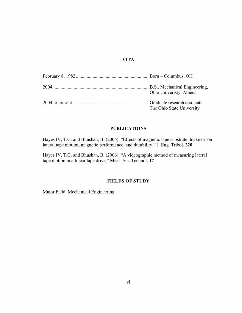
VITA February 8, 1982 ..............................................................Born – Columbus, OH
2004..................................................................................B.S., Mechanical Engineering, Ohio Univeristy, Athens
2004 to present.................................................................Graduate research associate The Ohio State University
PUBLICATIONS Hayes IV, T.G. and Bhushan, B. (2006). “Effects of magnetic tape substrate thickness on lateral tape motion, magnetic performance, and durability,” J. Eng. Tribol. 220
Hayes IV, T.G. and Bhushan, B. (2006). “A videographic method of measuring lateral tape motion in a linear tape drive,” Meas. Sci. Technol. 17
FIELDS OF STUDY
Major Field: Mechanical Engineering
vii
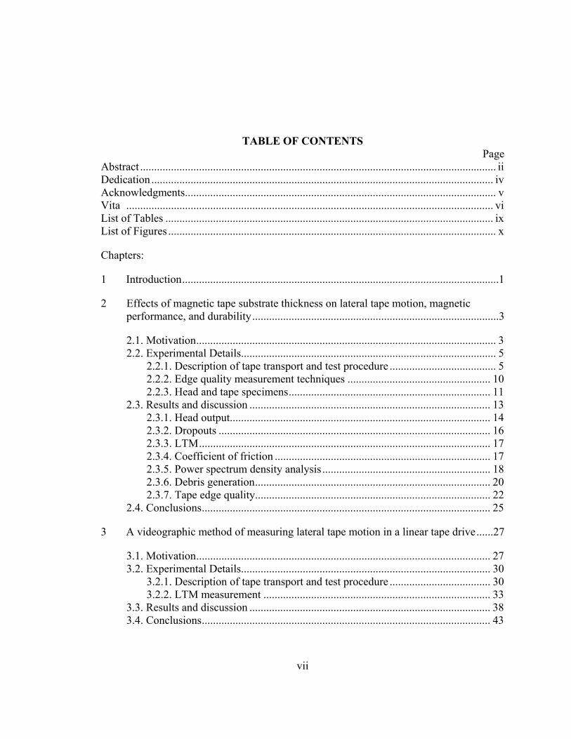
TABLE OF CONTENTS Page
Abstract ............................................................................................................................... ii Dedication .......................................................................................................................... iv Acknowledgments............................................................................................................... v Vita ................................................................................................................................... vi List of Tables ..................................................................................................................... ix List of Figures ..................................................................................................................... x
Chapters:
1 Introduction.................................................................................................................1
2 Effects of magnetic tape substrate thickness on lateral tape motion, magnetic performance, and durability........................................................................................3
2.1. Motivation........................................................................................................... 3 2.2. Experimental Details........................................................................................... 5
2.2.1. Description of tape transport and test procedure ...................................... 5 2.2.2. Edge quality measurement techniques ................................................... 10 2.2.3. Head and tape specimens........................................................................ 11
2.3. Results and discussion ...................................................................................... 13 2.3.1. Head output............................................................................................. 14 2.3.2. Dropouts ................................................................................................. 16 2.3.3. LTM........................................................................................................ 17 2.3.4. Coefficient of friction ............................................................................. 17 2.3.5. Power spectrum density analysis............................................................ 18 2.3.6. Debris generation.................................................................................... 20 2.3.7. Tape edge quality.................................................................................... 22
2.4. Conclusions....................................................................................................... 25
3 A videographic method of measuring lateral tape motion in a linear tape drive......27
3.1. Motivation......................................................................................................... 27 3.2. Experimental Details......................................................................................... 30
3.2.1. Description of tape transport and test procedure .................................... 30 3.2.2. LTM measurement ................................................................................. 33
3.3. Results and discussion ...................................................................................... 38 3.4. Conclusions....................................................................................................... 43
viii
4 Vibration analysis of axially moving magnetic tape with comparisons to static and dynamic experimental results.............................................................................47
4.1. Motivation......................................................................................................... 47 4.2. Sources of LTM................................................................................................ 49 4.3. Vibration model ................................................................................................ 51
4.3.1. Natural frequency analysis ..................................................................... 55 4.3.2. Modal analysis........................................................................................ 56
4.4. Experimental details ......................................................................................... 57 4.4.1. Description of the dynamic test apparatus and test procedure ............... 57 4.4.2. Static test apparatus ................................................................................ 58
4.5. Results and discussion ...................................................................................... 60 4.5.1. Simulation............................................................................................... 60 4.5.2. Dynamic measurement ........................................................................... 68 4.5.3. Static measurement................................................................................. 70
4.6. Conclusions....................................................................................................... 70
5 Summary ...................................................................................................................75
Appendices: A Droupout counter code............................................................................................. 77 B Droupout counter noise reducing trigger circuit ...................................................... 87 C PSD spectrum matlab code ...................................................................................... 88 D Videographic analysis matlab code ....................................................................... 105 E Vibration model matlab code................................................................................. 108 Bibliography ................................................................................................................... 115
ix
LIST OF TABLES
Table Page
4.1 Parameters studied for 6.5 µm tape with the nominal conditions in bold. ........... 58
4.2 Parameters studied with the nominal conditions in bold. ..................................... 61
4.3 Physical properties for tapes of varying thickness................................................ 61
4.4 First ten calculated natural frequencies in Hz while varying axial velocity, tension, free span length, and tape thickness. With the exception of the parameter being studied in the table the natural frequencies were calculated with the following parameters: 6 m/s, 0.5 N, 0.5 m, and 6.5 µm ........ 62
4.5 First natural frequency for stationary tape with a free span of (a) 0.5 m and (b) 1.0 m................................................................................................................ 72
x
LIST OF FIGURES
Figure Page 2.1 Schematic of the tape transport showing LTM probe location and cross-
section of the stationary guides. (Goldade and Bhushan, 2003)............................. 6
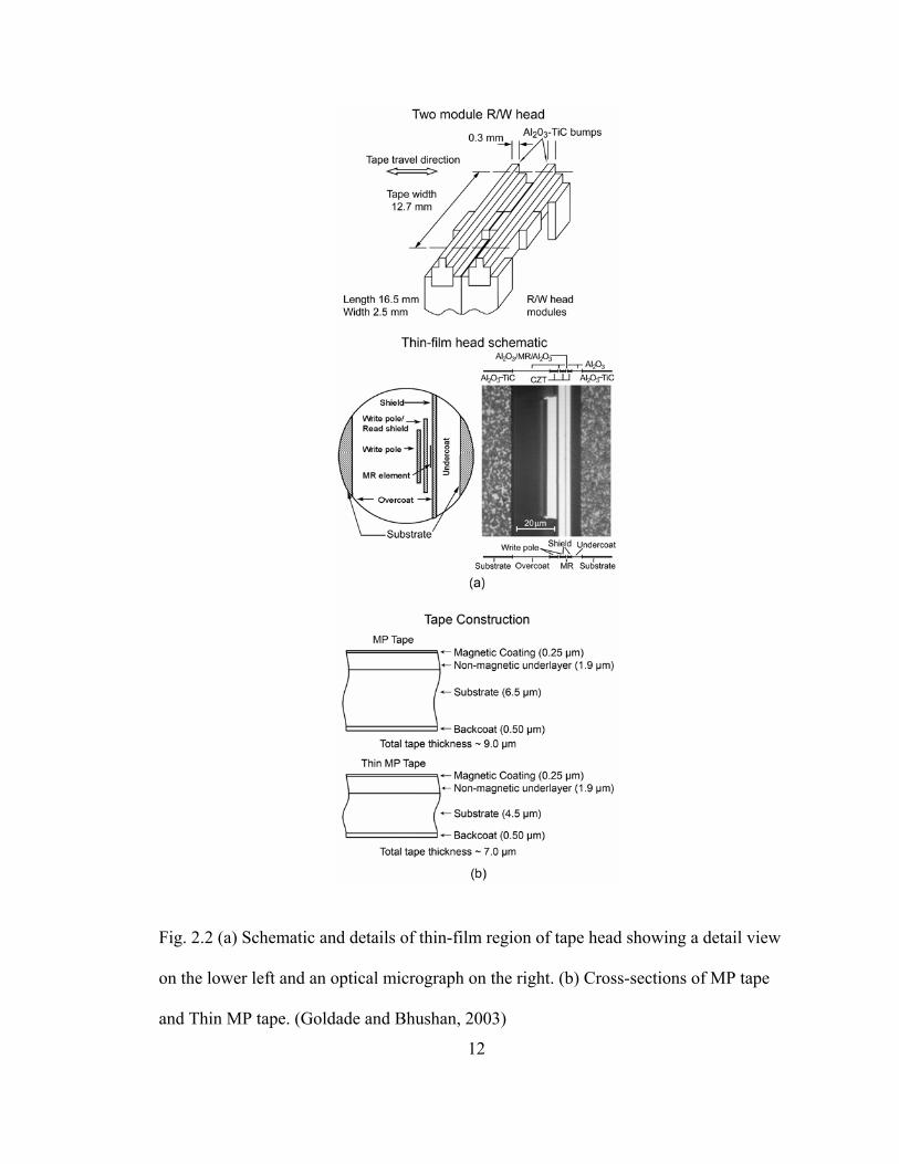
2.2 (a) Schematic and details of thin-film region of tape head showing a detail view on the lower left and an optical micrograph on the right. (b) Cross-sections of MP tape and Thin MP tape. (Goldade and Bhushan, 2003) ............... 12
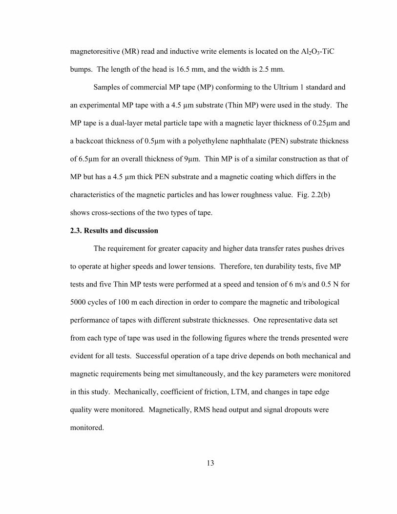
2.3 Head output, number of dropouts per cycle, LTMP amplitude, and coefficient of friction versus number of cycles for MP and Thin MP tapes......... 15
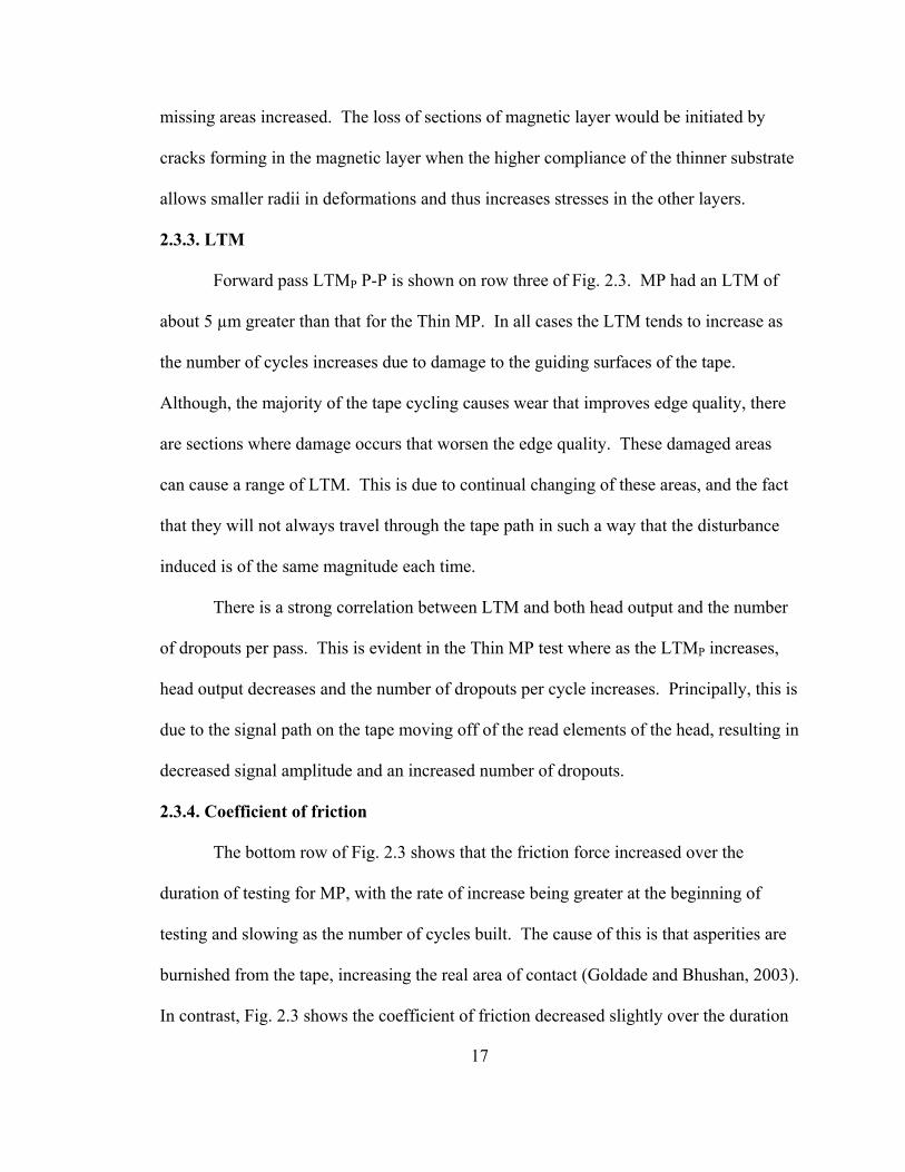
2.4 (a) Comparison of power spectrum densities for MP and Thin MP tapes before and after 5000 cycles (b) Comparison of the coherence between the top edge probe signal and bottom edge probe signal for MP and Thin MP tapes before and after 5000 cycles. ....................................................................... 19
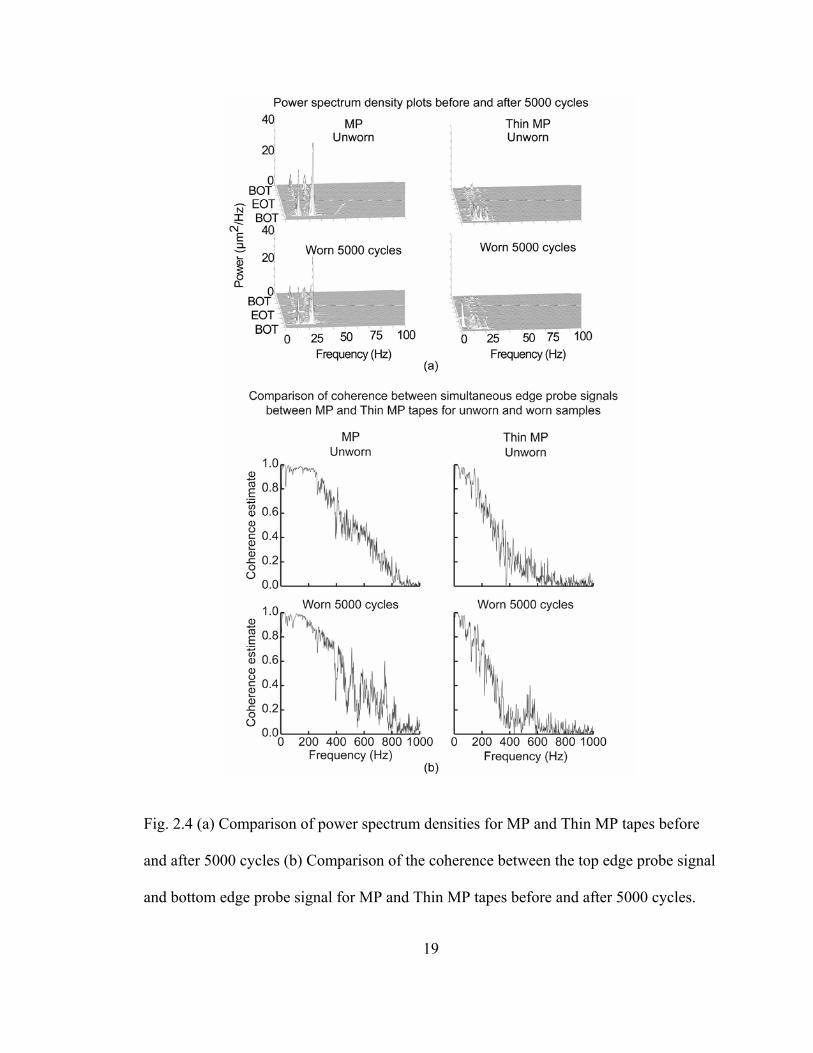
2.5 Optical micrographs of the tape heads for MP and Thin MP tapes showing debris accumulation in the area of the tape edge. ................................................. 21
2.6 Optical micrographs of top and bottom tape edges for both the magnetic coat and backcoat sides, with edge contour lines obtained through image processing shown above and below the respective micrograph. .......................... 23
2.7 Summary of relative edge contour length results showing deviation of the edge contour length from a perfectly straight edge. ............................................. 24
3.1 Schematic illustrating the different components of LTM and their contribution to the total LTM measurement (Alfano and Bhushan, 2006a)......... 29
3.2 Schematic of the tape transport showing LTM probe location and cross-section of the stationary guides (Goldade and Bhushan, 2003)............................ 31
3.3 Schematic showing detail of the optical edge probe measurement technique (Goldade and Bhushan, 2003) .............................................................. 34
3.4 Comparison of standard and scratching tape paths showing camera location in relation to the tape deck ...................................................................... 36
xi
3.5 Graphical representation of the analysis process for a single frame of video...................................................................................................................... 39
3.6 LTM mean total amplitude (ATM) data plot for both the edge probe and videographic methods ........................................................................................... 40
3.7 Real-time plot of data from the edge probe and videographic methods ............... 42
3.8 PSD plots showing the frequency components contained in the data from the edge probe (top) and the videographic (bottom) methods .............................. 44
4.1 Schematics to illustrate common sources of LTM. (a) Effect of reel tilt amplitude on tape guiding. Reel and guide misalignment can cause harmonic excitation of the tape and apply side forces to the tape edge, resulting in further unwanted LTM. (b) Effect of staggered wraps on tape guiding. Staggered wraps, formed through improper winding of the tape, can cause very high LTM as the wrap unwinds during operation. (Boyle and Bhushan, 2006) .............................................................................................. 50
4.2 (a) Reduction of the tape path to a schematic representation of the system (b) Final simplification into a fixed-fixed Euler-Bernoulli beam model with axial velocity V............................................................................................. 53
4.3 The static test apparatus used to study the effects of free span length, tape thickness, and tension of the first natural frequency by directly exciting the tape........................................................................................................................ 59
4.4 Effects of varying the operating parameters on the first natural frequency for (a) axial velocity, (b) tension, (c) free span, and (d) tape thickness. (a) As the axial velocity increases, the natural frequencies decrease until the first natural frequency goes to zero. (b) Increasing tension results in the natural frequencies increasing in an approximately linear manner. (c) For free spans less than 0.5 m the natural frequencies increase rapidly with decreasing free span length. (d) Natural frequencies decrease as thickness is increased............................................................................................................ 64
4.5 The first four mode shapes with varying axial velocities. Increasing axial velocity results in real components of the mode shapes being shifted in the direction of motion, to the right, and increases the amplitude of successive peaks. The opposite is true for the imaginary components of the mode shapes in regards to both shifting and amplitude in successive peaks.................. 67

xii
4.6 Study of the effects of varying tension and velocity on the frequency components of dynamic tape. Excited modes corresponding to the reel to reel free span length can be seen in each plot. ...................................................... 69
4.7 Amplitude ratio versus frequency for the static test as tension, free span length, and tape thickness are varied with three values of tension shown in each plot. The value of the first natural frequency increases with increased tension and decreases with increased free span length as predicted by the vibration model. ......................................................................... 71
B.1 A circuit built around a single LM324 quad op-amp circuit to reject voltage spikes in the tension transducer signal as the drive starts and stops. ....... 87
1
CHAPTER 1
INTRODUCTION
Nearly all digital data is stored on magnetic media. Magnetic media includes
magnetic tape, hard drives, and floppy disks. Hard drives are used for storage of large
amounts of data, up to 750 GB for a 3.5 inch drive as of this writing, and can access that
data quickly. Compared to magnetic tape, hard drives are still an expensive method of
storing data on a per gigabyte basis when terabytes of data need to be stored. Magnetic
tape is used as a long term backup solution where quick access is not needed and the
maximum capacity is required. Currently, a single cartridge of Sony SAIT can store 500
GB natively and 1.3 TB compressed (Anonymous, 2004). Floppy disks are nearly
obsolete but still provide a simple way to store a small amount of data.
All three of these technologies require a head with read/write elements to be in
close proximity of the magnetic media in relative motion. The closer the read/write
elements are to the media, the narrower the data track that can be written due to the
magnetic fields being less diffuse. By reducing the head-to-media spacing, contact
between the media and head becomes a concern and a likely mode of failure. In order to
maximize the life of the media, there is usually a layer of diamond-like carbon (DLC)
covered in a thin layer of lubricant.
2
Lateral tape motion (LTM) is a topic of special concern to magnetic tape. LTM is
the unwanted relative motion of the tape parallel to the head. As tracks become narrower
in magnetic tape, the tolerance of LTM becomes smaller as well. If LTM is of too great a
magnitude, it can cause errors during both reading and writing. During reading, the drive
can lose the data track and must try again to read the data. If LTM occurs during writing,
there is the possibility of overwriting data. Steps in drive design have been taken to
minimize the likelihood of these errors, but errors are still possible.
In order to minimize LTM, it is necessary to understand what causes LTM and the
effects it has. Chapter 2 focuses on the durability of magnetic tape both magnetically and
tribologically and investigates the tape as the source of LTM where the thickness of the
substrate is taken into consideration as well as the condition of the tape edges. Measuring
LTM has also proven to be an elusive task. Traditionally, optical edge probes have been
used to measure the position of the tape edge, but due to edge damage and the tendency
of the tape to follow the same path on each pass, this measurement has been called into
question. A videographic technique is investigated in Chapter 3 for the measurement of
LTM by creating a reference line on the tape which is then monitored. The results of the
videographic method are compared to those of the edge probe. Finally, in order to
understand the basic mechanics behind LTM, a vibration model is developed which takes
axial motion into account and is used to investigate the effects of axial velocity, tension,
free span length, and tape thickness. The results of the model are compared to both
dynamic and static, with and without axial motion, experimental tests in Chapter 4.

3
CHAPTER 2
EFFECTS OF MAGNETIC TAPE SUBSTRATE THICKNESS ON LATERAL TAPE MOTION, MAGNETIC PERFORMANCE, AND DURABILITY
2.1. Motivation
Capacities of magnetic tape are currently 400 GB (800 GB compressed) for LTO
Ultrium 3 and 500 GB (1 TB compressed) for SAIT (Anonymous, 2005, 2004). In order
to create a multi-terabyte capacity cartridge, manufacturers are increasing the areal data
density as well as the volumetric density (Bhushan, 1996). Increasing the areal density
results in higher capacity for a given volume of tape by decreasing both the track pitch
and the length of a bit. By using a thinner substrate and coatings, a greater length of tape
can be wound on a cartridge, thereby increasing data capacity for a given volume.
Decreasing the thickness of the substrate places greater stress on the substrate as well as
creating a higher compliance tape. Both of these factors can increase the chances of
damage to the coatings through cracking due to increased strain and buckling of the tape
in situations that were not a problem with thicker substrates.
As the areal density increases, the head-to-tape spacing must decrease in order to
maintain an acceptable signal-to-noise ratio and resolution (Bhushan, 1996). This
requires the tape to be smoother to minimize the asperity-induced head-to-tape spacing.
A side effect of having a smooth tape is that the coefficient of friction increases due to a
4
higher real area of contact and greater compliance (Bhushan, 2000). To reduce the
effects of the increased coefficient of friction, the tension is reduced, but this has the
negative effect of increasing the flying height of the tape over the heads and guides since
the hydrodynamic forces are affected to a lesser degree by the thickness of the substrate
(Elrod and Eshel, 1965). Potentially, the tape path becomes less stable, and lateral tape
motion (LTM) becomes greater as the flying height increases due to reduced frictional
forces that would otherwise dampen the motion. This is a problem because if LTM
becomes excessive, the tape will move the data track away from the read/write elements
of the head causing a track misregistration (TMR). In practice, the frequency of TMR is
reduced in a commercial drive with a servo mechanism that follows a servo track written
at the time of manufacture and reduces the effect an LTM event has on data retrieval.
These tracking mechanisms have a limited bandwidth, typically less than 1 kHz, and
TMR may still occur if the LTM event is of significant amplitude and accelerates faster
than the servo mechanism can track it (Richards and Sharrock, 1998). The track widths
in next generation data patterns are narrower, which means that they have even less
tolerance of LTM before TMR occurs (Richards and Sharrock, 1998; Goldade and
Bhushan, 2003; Wang et al., 2003).
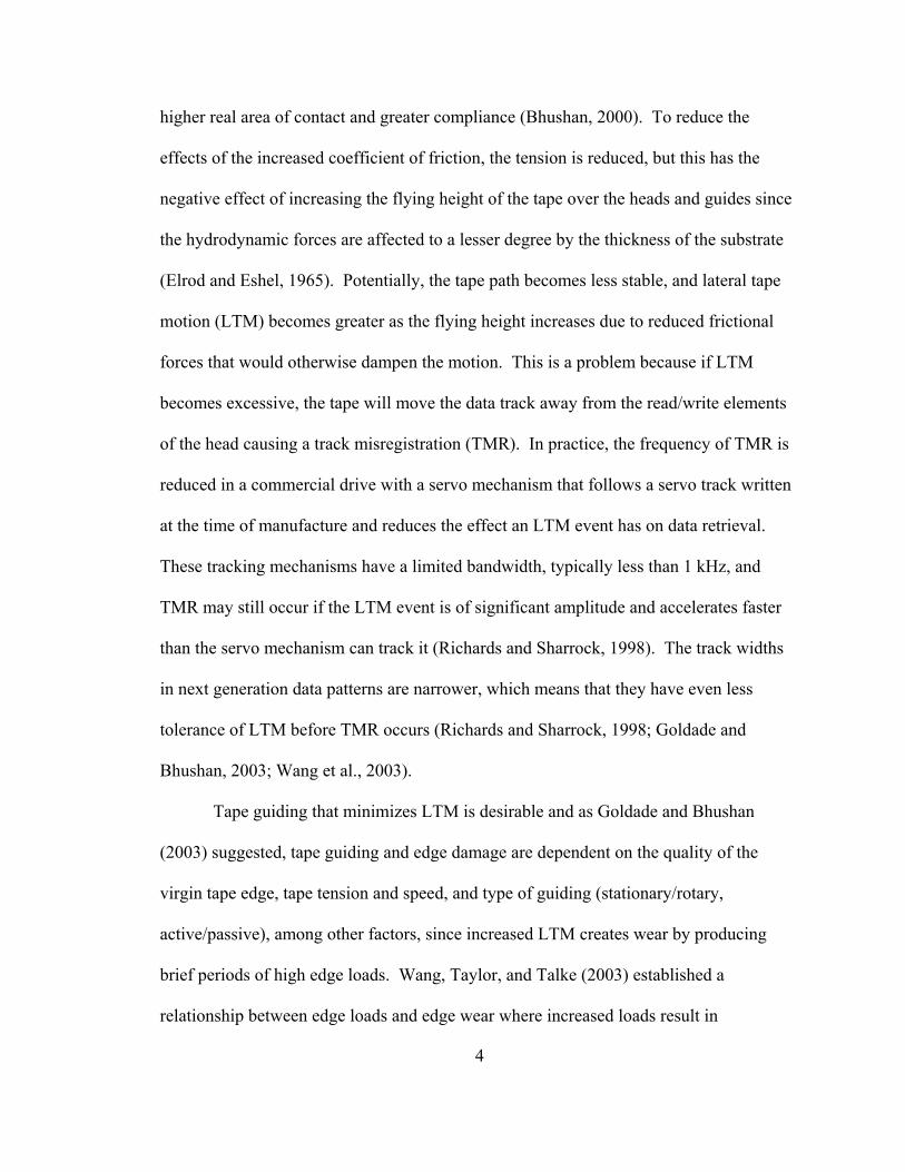
Tape guiding that minimizes LTM is desirable and as Goldade and Bhushan
(2003) suggested, tape guiding and edge damage are dependent on the quality of the
virgin tape edge, tape tension and speed, and type of guiding (stationary/rotary,
active/passive), among other factors, since increased LTM creates wear by producing
brief periods of high edge loads. Wang, Taylor, and Talke (2003) established a
relationship between edge loads and edge wear where increased loads result in
5
disproportionately increased wear. Goldade and Bhushan (2004) also suggested that
damage to the tape edge may result in increased LTM. Increased LTM results in tracking
problems as the lateral acceleration of the tape exceeds the servo mechanism’s
capabilities and higher edge loads. Higher edge loads result in increased wear and debris.
As this debris enters the head to tape interface read/write errors can occur due to head-to-
tape spacing that is too large.
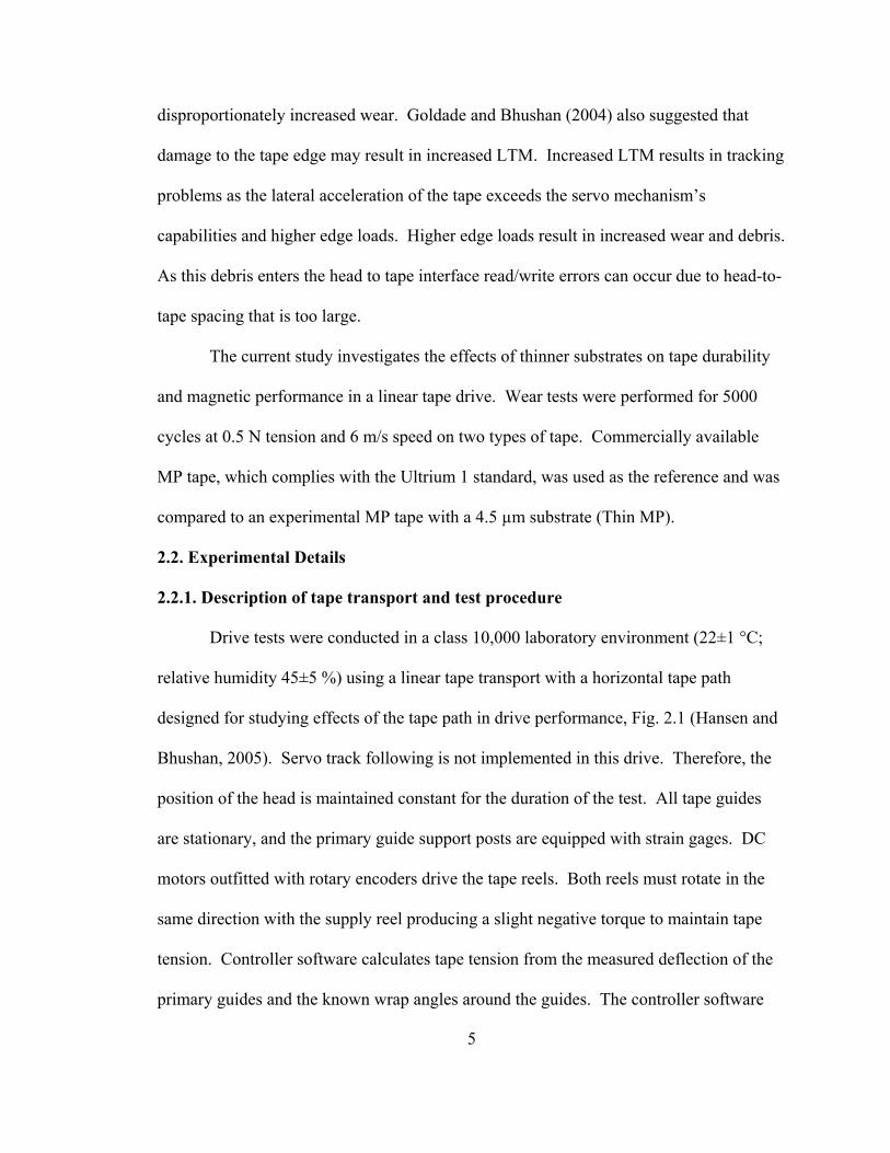
The current study investigates the effects of thinner substrates on tape durability
and magnetic performance in a linear tape drive. Wear tests were performed for 5000
cycles at 0.5 N tension and 6 m/s speed on two types of tape. Commercially available
MP tape, which complies with the Ultrium 1 standard, was used as the reference and was
compared to an experimental MP tape with a 4.5 µm substrate (Thin MP).
2.2. Experimental Details
2.2.1. Description of tape transport and test procedure
Drive tests were conducted in a class 10,000 laboratory environment (22±1 °C;
relative humidity 45±5 %) using a linear tape transport with a horizontal tape path
designed for studying effects of the tape path in drive performance, Fig. 2.1 (Hansen and
Bhushan, 2005). Servo track following is not implemented in this drive. Therefore, the
position of the head is maintained constant for the duration of the test. All tape guides
are stationary, and the primary guide support posts are equipped with strain gages. DC
motors outfitted with rotary encoders drive the tape reels. Both reels must rotate in the
same direction with the supply reel producing a slight negative torque to maintain tape
tension. Controller software calculates tape tension from the measured deflection of the
primary guides and the known wrap angles around the guides. The controller software
6
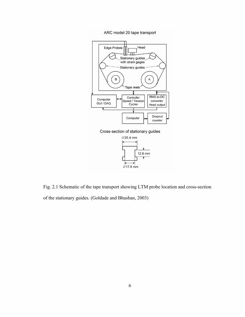
Fig. 2.1 Schematic of the tape transport showing LTM probe location and cross-section
of the stationary guides. (Goldade and Bhushan, 2003)
7
samples the rotary encoders every millisecond to calculate the motor angular speed and
maintains constant average tape tension throughout the pass. Tape is loaded onto a reel
until the diameter of the pack is 60 mm. Controller software calculates tape linear
velocity from reel angular velocity and original tape pack diameter and maintains
constant linear speed throughout the pass. The pass length was set at 100 m for all tests,
with one forward and reverse pass equal to one 200 m cycle. Nominal speed and tension
were 6 m/s and 0.5 N.
LTM was measured using two fiber-optic edge displacement probes (sensitivities
of 17.85 µm/V and 14.72 µm/V and noise levels of 20 mVP-P). The edge probes were
placed as close as possible to the head on the reel B side with one probe monitoring the
top edge while the second probe monitored the bottom edge. Light from the light source
built into the probe module is directed into a fiber optic cable where it is guided to a 90°
prism and reflected to another 90° prism where it is directed through another fiber optic
cable finally reaching a photodiode (light receiver) in the probe module. The sensor
converts the photodiode signal, which is proportional to the light intensity, into the output
units (volts or microns). If the light path is not obstructed by the tape edge, the output of
the sensor is 100%. The output decreases as the tape moves upward into the gap between
the prisms and diminishes to zero when no light reaches the photodiode. The transfer
curve has a linear region in the center of which the reference point is selected
corresponding to “zero” lateral displacement.
Optical measurements of LTM, such as with the edge probes used, convolve tape
motion measurement with measurement of the tape edge profile. Because the output
voltage of the probe is proportional to the amount of light received by the photodiode,
8
variations in both the tape edge contour and the tape edge position are measured
simultaneously. Measuring LTM at the upper and lower edges of the tape simultaneously
and comparing these signals give some means of separating the edge contour information
from the edge motion measurement. Goldade and Bhushan (2003) concluded that the
two edges of commercially slit tape are imperfect and different from each other.
Therefore, given that the upper and lower edges of the tape move together, differences in
the LTM signals obtained from the two edges are due solely to edge contours. If the two
signals change together equally, the tape has moved as a unit, and true LTM has been
measured. The coherence of the two signals was estimated using the Matlab “cohere”
function with a 1024-point fft. The coherence estimate ( ) 0=fCxy if the two signals are
completely incoherent (edge contour effects) at the frequency f, and ( ) 1=fCxy if the two
signals are fully coherent (LTM event) (Beauchamp and Yuen, 1979).
Wear tests were conducted on a sample of experimental Thin MP tape and a
sample of commercial MP tape. The same NS20 head was used for all tests. Before each
test the head was cleaned thoroughly with methyl alcohol and a lint free cloth. A new
piece of tape was loaded for each test and was cycled approximately 10 times before
testing began in order to find a clear area, write the signal, and adjust the output current
to the appropriate level. The signal written to the tape was a 5.9055 MHz sine wave
which has a recording density of 25 kfci. The drive was then programmed to run for
5000 cycles. Head output was split and sent to an RMS-to-DC converter (conversion
time is 181 ms) and a commercial dropout counter. A data acquisition board was used to
record the head output, primary guide strain gage signals (tension), and the edge probe
signals. Data acquisition was controlled by data acquisition software with the sampling
9
rate set to 100 Hz. A BASIC program on another computer controlled the dropout tester.
The dropout tester was triggered by a signal from the transport controller at the beginning
of each forward and reverse pass. After the test was completed, the tape was removed,
and a section was kept for further analysis.
Once a test was complete, the data collected during testing was analyzed using the
following methods. Head output and coefficient of friction were averaged over each pass
and plotted. Head output data was converted to a voltage decibel format. The reference
voltage is the average of the head output voltage for the first 10 cycles. Coefficient of
friction across the head was calculated using the belt equation using the tension signals
obtained from the strain gages and the known geometry of the tape path. See Bhushan
and Mokashi (2001) for details of the calculation. The head wrap angle was 30°, and the
guide wrap angle was 48°. Head output and tension signals were recorded with the DAQ.
Physical LTM peak-to-peak amplitude (LTMP P-P amplitude) was calculated by
dividing the pass into four equal sections of approximately 20 m and finding the
difference between the highest and lowest value in each of the four sections. The initial
and final 10 m were neglected in order to allow the drive to reach steady state before
measurements were taken. Next, these four sections were averaged to reduce the effects
of an unusually high peak in one section of tape combining with an unusually low valley
in another section to create a peak-to-peak value that is not representative. LTM is also
presented in power spectrum density (PSD) plots for five passes before and after the 5000
cycle test where the sampling rate was 1000 Hz. PSD is calculated using a program that
parsed the LTM data into one second blocks, performs a fast Fourier transform on each
block, and calculates the power contained at interval frequencies for the entire cycle. The
10
resulting PSD plot was very repeatable for each set of cycles before and after the 5000
cycles, so only one plot is presented on behalf of the others.
Dropouts were monitored as a way of quantifying magnetic performance and to
provide insight into the mechanical durability of the magnetic coating for the duration of
the test. Due to the higher compliance of a thin substrate, the magnetic layer may be
over-stressed and develop cracks, ultimately resulting in loss of sections of magnetic
layer. A dropout is a head signal loss of a defined duration and magnitude. Dropouts are
caused by a variety of sources including LTM, tape defects, local demagnetization,
asperities on the tape, debris entering the head-to-tape interface, and any other event that
causes an increase of the head-to-tape spacing (Alstad and Haynes, 1978; Anderson and
Bhushan, 1996). The number and magnitude of dropouts was measured with the dropout
tester. Twenty classes of dropouts are defined by the amplitude of signal loss and the
duration of signal loss. Dropout depth and duration are selectable in the ranges of 1-22
dB in 0.5 dB increments and 0.5-300 µs in 0.5 µs increments. Dropout parameters used
in this study were: >4-6, >6-9, >9-12, and >12 dB; >0.5-1, >1-5, >5-10, >10-25, and >25
µs. The number of dropouts was counted during each forward and reverse pass. After
the test was complete, the number of dropouts was calculated and plotted for the forward
pass.
2.2.2. Edge quality measurement techniques
The edges of the tapes used in wear testing were analyzed before use in the tape
drive and after 5000 cycles using optical microscopy. The notations “upper edge” and
“lower edge” are assigned according to how the tape was loaded into the transport, with

11
the lower edge being the edge close to the base of the transport. Each edge was imaged
from both the magnetic and backcoat side of the tape.
Tape samples were cut into 30 mm strips and mounted on glass microscope slides
with double-sided adhesive tape. Optical images were obtained in the brightfield mode
with a white light source, and gray-scale images (640×480 pixels) were captured with a
CCD camera at a resolution of 0.175 µm per pixel.
Edge quality measurements were performed using the methodology developed by
Topoleski and Bhushan (2000) and Goldade and Bhushan (2003, 2004). Relative edge
contour length is a measure of edge quality. The tape edge appears in the optical
micrograph as a line of pixels of varying opacity. Adding power to the light source of the
microscope overexposes the image, leaving behind the tape edge as the transition
between the bright area of the image caused by the overexposure of the tape and the
darker region of the background. With the use of image analysis software, the edge
contour is outlined, and the number of pixels constituting the edge is calculated. The
total number of pixels for each edge is divided by the number of pixels for a perfectly
straight line to obtain the relative edge contour length. Relative edge contour length is a
measure of the deviation of the tape edge from a perfectly straight line (110µm). Each
relative edge contour length measurement reported is the average of ten measurements.
2.2.3. Head and tape specimens
A commercial NS20 two module read/write head was used. The schematic of the
head along with the thin-film structure are shown in Fig. 2.2(a). The two read/write
modules are embedded in an aluminum housing. The thin-film region containing the
12
Fig. 2.2 (a) Schematic and details of thin-film region of tape head showing a detail view
on the lower left and an optical micrograph on the right. (b) Cross-sections of MP tape
and Thin MP tape. (Goldade and Bhushan, 2003)
13
magnetoresitive (MR) read and inductive write elements is located on the Al2O3-TiC
bumps. The length of the head is 16.5 mm, and the width is 2.5 mm.
Samples of commercial MP tape (MP) conforming to the Ultrium 1 standard and
an experimental MP tape with a 4.5 µm substrate (Thin MP) were used in the study. The
MP tape is a dual-layer metal particle tape with a magnetic layer thickness of 0.25µm and
a backcoat thickness of 0.5µm with a polyethylene naphthalate (PEN) substrate thickness
of 6.5µm for an overall thickness of 9µm. Thin MP is of a similar construction as that of
MP but has a 4.5 µm thick PEN substrate and a magnetic coating which differs in the
characteristics of the magnetic particles and has lower roughness value. Fig. 2.2(b)
shows cross-sections of the two types of tape.
2.3. Results and discussion
The requirement for greater capacity and higher data transfer rates pushes drives
to operate at higher speeds and lower tensions. Therefore, ten durability tests, five MP
tests and five Thin MP tests were performed at a speed and tension of 6 m/s and 0.5 N for
5000 cycles of 100 m each direction in order to compare the magnetic and tribological
performance of tapes with different substrate thicknesses. One representative data set
from each type of tape was used in the following figures where the trends presented were
evident for all tests. Successful operation of a tape drive depends on both mechanical and
magnetic requirements being met simultaneously, and the key parameters were monitored
in this study. Mechanically, coefficient of friction, LTM, and changes in tape edge
quality were monitored. Magnetically, RMS head output and signal dropouts were
monitored.

14
2.3.1. Head output
As shown in the first row of Fig. 2.3, head output stayed within ±2 dB for all
tests. There did not appear to be any trend either increasing or decreasing for head output
for either type of tape which agrees with previous results presented by Hansen and
Bhushan (2005) where the effects of speed and tension on MP tape were investigated.
Note that the signal has been normalized by conversion to dB using the average of the
first five passes as the reference level, so direct comparison between the two tapes is
more readily made.
Thin MP does tend to exhibit a more erratic signal than MP does. This is
attributed to head-to-tape spacing, formulation, and debris. Since Thin MP is more
compliant, its head-to-tape spacing in more likely to fluctuate than that of MP which is
less compliant and flies at a more consistent height. Signal losses result when head-to-
tape spacing increases. The formulation of the tapes is also a contributing factor since the
strength of the signal induced in the head, and ultimately the signal seen by the data
acquisition system, depends on the magnetic particles used in the magnetic layer. As the
tape is cycled, damage occurs, and debris is shed that causes the majority of the erratic
head output fluctuations seen in Fig. 2.3 through a process where debris accumulates in
the head-to-tape interface, increasing head-to-tape spacing and thus reducing head output.
Periodically, these accumulations will be cleared by the rubbing of the tape traveling over
it, and new deposits will begin to form again. This process occurs in such a way that it is
not dependent on the number of passes, and the frequency and magnitude of the
disturbances are unpredictable (Hansen and Bhushan, 2005). LTM also causes
15
Fig. 2.3 Head output, number of dropouts per cycle, LTMP amplitude, and coefficient of
friction versus number of cycles for MP and Thin MP tapes.
16
fluctuations in head output when the written signal moves away from read element on the
head.
2.3.2. Dropouts
As a metric of magnetic performance and durability of the magnetic layer, the
number of dropouts per pass was monitored. The dropout tester can measure twenty
classes of dropouts defined by ranges of signal loss magnitude and duration. Dropouts
were counted in every class with the majority of counts in the >4-6 dB and 0.5-1 µs.
Summing across the range of classes and plotting the logarithm of resulting number per
pass was used to create the plots shown in the second row of Fig. 2.3.
The number of dropouts correlates to areas of erratic head output where the output
drops below 0 dB. There are areas where the number of dropouts increases when head
output increases, and areas where the number of dropouts does not increase when the
head output decreases. This is explained by the fact that the dropout counter is
monitoring signal quality and auto-ranges for each pass compensating for persistent
changes in signal magnitude. In addition, the head output is an average across the entire
length of the pass and is not able to illustrate the short term signal fluctuations
responsible for the majority of dropouts.
Since the number of dropouts remains nearly constant, the mechanical durability
of the magnetic layer of the thin MP tape is determined to be comparable to that of MP
tape. If mechanical durability was not sufficient, it would be manifested by an increase
in dropouts due to a local loss of sections of magnetic layer, and the number of dropouts
would gradually increase as more areas of magnetic layer were lost and the size of these
17
missing areas increased. The loss of sections of magnetic layer would be initiated by
cracks forming in the magnetic layer when the higher compliance of the thinner substrate
allows smaller radii in deformations and thus increases stresses in the other layers.
2.3.3. LTM
Forward pass LTMP P-P is shown on row three of Fig. 2.3. MP had an LTM of
about 5 µm greater than that for the Thin MP. In all cases the LTM tends to increase as
the number of cycles increases due to damage to the guiding surfaces of the tape.
Although, the majority of the tape cycling causes wear that improves edge quality, there
are sections where damage occurs that worsen the edge quality. These damaged areas
can cause a range of LTM. This is due to continual changing of these areas, and the fact
that they will not always travel through the tape path in such a way that the disturbance
induced is of the same magnitude each time.
There is a strong correlation between LTM and both head output and the number
of dropouts per pass. This is evident in the Thin MP test where as the LTMP increases,
head output decreases and the number of dropouts per cycle increases. Principally, this is
due to the signal path on the tape moving off of the read elements of the head, resulting in
decreased signal amplitude and an increased number of dropouts.
2.3.4. Coefficient of friction
The bottom row of Fig. 2.3 shows that the friction force increased over the
duration of testing for MP, with the rate of increase being greater at the beginning of
testing and slowing as the number of cycles built. The cause of this is that asperities are
burnished from the tape, increasing the real area of contact (Goldade and Bhushan, 2003).
In contrast, Fig. 2.3 shows the coefficient of friction decreased slightly over the duration

18
of testing for Thin MP. In this case, the tape has a smoother magnetic coating and
exhibited an initial coefficient of friction approximately fifty percent greater than that for
MP. As the tape was cycled, debris was generated by the tape edges and worked its way
to the tape surface where it acted as a solid lubricant reducing friction at the head-to-tape
interface.
2.3.5. Power spectrum density analysis
Figure 2.4(a) shows the power spectrum density (PSD) plots for MP and Thin MP
before and after 5000 cycles. The PSD plots show that for both tapes, nearly all the
power is present below 60 Hz, with the higher frequency components being produced by
periodic perturbations caused by the reels (Hansen and Bhushan, 2005). Frequencies
present in MP tape form two distinct bands at approximately 25 Hz and 45 Hz. Thin MP
tape forms three frequency bands at approximately 20 Hz, 25 Hz, and 30 Hz that are, on
average, half the power of MP. After 5000 cycles, both MP and Thin MP show a
reduction of approximately fifty percent for the power present.
The use of dual edge probes allows the calculation of a coherence estimate for
how well the signal acquired by each probe correlates with that from the other. If the two
signals are coherent, it can be concluded that the motion reported by the edge probes is
real motion since both edges moved the same amount in the same amount of time. Figure
2.4(b) shows that MP tape exhibits coherence across a broader range than Thin MP does.
In this case MP has coherence near 1.0 for the first 200 Hz and Thin MP exhibits a high
level of coherence to 150 Hz. Both tapes slope down to near zero, no coherence, at 900
Hz. Figure 2.4(b) also shows that after 5000 cycles, the bandwidth of coherence
decreases to only the lowest frequencies and both tapes become incoherent by 700 Hz.
19
Fig. 2.4 (a) Comparison of power spectrum densities for MP and Thin MP tapes before
and after 5000 cycles (b) Comparison of the coherence between the top edge probe signal
and bottom edge probe signal for MP and Thin MP tapes before and after 5000 cycles.

20
This indicates that for frequencies below 200 Hz, most of the motion of the tape is real
motion. As the number of cycles builds this level of coherence is reduced until there is
only a small region of coherence. This indicates that the edges of the tape are no longer
moving the same amount at the same time. The reduced bandwidth of coherence for Thin
MP is most likely caused by a combination of the tape rigidity and initial edge quality. A
more flexible tape is less likely to emulate a rigid beam in its motions in that it is less
likely to move up and down as a unit since it is easier for it to buckle. Also, the initial
edge quality plays a roll in that variations in the edge are convolved into the signal
resulting in a decrease in coherence since the edge quality is a random occurrence as
opposed to an LTM event which would be identical between the two signals.
2.3.6. Debris generation
Figure 2.5 shows micrographs of the head after 5000 cycles for both MP and Thin
MP tapes. MP created a small amount of debris that is most conspicuous on the head
above the area of the upper tape edge. The tape edge locations are dark strips that run
across the width of the head, caused by the contact of the tape edges creating a streak of
very fine debris. A small amount of debris can also be made out along the edges of the
Al2O3-TiC head bumps varying from light to dark gray. Thin MP created much more
debris both deposited on the head surface and along the sides of the head bumps. Thin
MP was also more likely to deposit fine debris on the running surface of the head as can
be seen as small dark streaks on the head in the upper right hand image. According to
Goldade and Bhushan (2003), this would indicate a poorer initial edge quality.
21
Fig. 2.5 Optical micrographs of the tape heads for MP and Thin MP tapes showing debris
accumulation in the area of the tape edge.

22
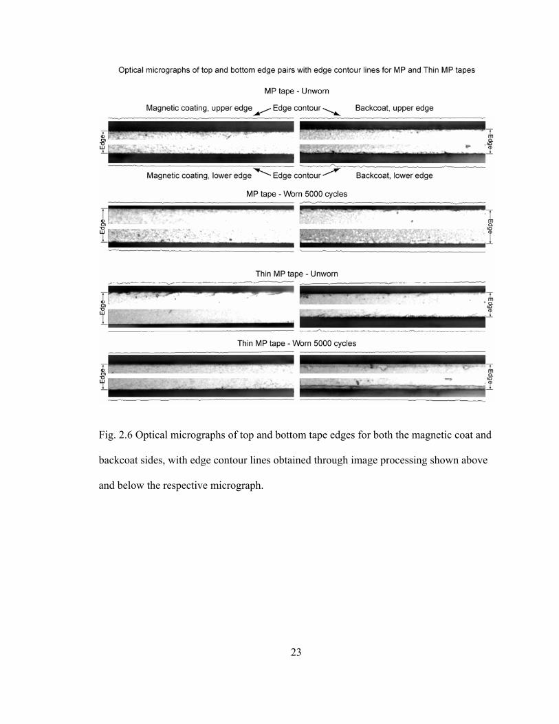
2.3.7. Tape edge quality
Optical micrographs were also taken of both tapes before and after cycling to
monitor changes in tape edge quality. Figure 2.6 shows images with edge contour lines
comparing unworn tape to tape worn 5000 cycles. Figure 2.6 is composed of upper edge
and lower edge pairs for both the magnetic coating and the backcoat sides of the tape.
Image analysis yields the edge contour lines of these edges. These edge contour lines are
shown above the upper edge and below the lower edge, respectively. These edge contour
lines are used to calculate a relative edge contour length which is the deviation from a
perfectly straight edge.
Averages of twenty images of each tape location were used to create a
comparison of the relative edge contour lengths for Fig. 2.7. The magnetic side of MP
increases its relative edge contour length (RECL) slightly, while the backside sees a more
pronounced decrease. Thin MP begins with a greater RECL and at three of the four
locations, experiences a decrease in RECL with the remaining edge exhibiting only a
minor increase in RECL. It is not surprising to see that the RECL for Thin MP decreased
much more than MP since MP had a better edge to begin with (near 1.05) and Thin MP
was closer to 1.08.
This suggests that a certain amount of edge damage is inevitable. Otherwise, the
RECL would have always approached 1.0, indicating a perfectly straight line. While
edge damage is inevitable, it does seem to approach a limit. In other words, if the tape
exhibits a good initial edge quality, it is more likely to exhibit a poorer edge quality after
cycling, and if the initial edge quality is initially poor, it is more likely to improve the
edge quality by removing the jagged edges, but this yields a greater amount of debris.
23
Fig. 2.6 Optical micrographs of top and bottom tape edges for both the magnetic coat and
backcoat sides, with edge contour lines obtained through image processing shown above
and below the respective micrograph.

24
Fig. 2.7 Summary of relative edge contour length results showing deviation of the edge
contour length from a perfectly straight edge.
25
2.4. Conclusions
This study has found that there are a couple of minor obstacles in moving to a
thinner substrate for future tapes. However, friction and debris generation tended to be
higher for Thin MP, and these characteristics should be addressed before Thin MP is
made a commercial product. On a more positive note, there was little-to-no impact on
magnetic performance in switching to a thinner substrate. Detailed conclusions follow.
Head output remained nearly constant for MP. Thin MP exhibited erratic signal
output after 2500 cycles. This is due to the periodic build up and removal of debris in the
head-to-tape interface and increased LTM. In Thin MP the asperities were of lesser
magnitude resulting in a greater signal loss when debris did enter the head-to-tape
interface.
The coefficient of friction showed opposite trends for each type of tape. In MP
the trend was upward, and this was caused by the burnishing of asperities and increasing
the real area of contact. For Thin MP, the coefficient of friction decreased over the
length of testing due to a greater amount of debris generation which acted as a solid
lubricant. Thin MP initially had a very smooth surface, and there was no burnishing
mechanism to counteract the effect of the debris particles.
Debris generation was a major difference between the performance of the two
tapes. Thin MP generated a much greater amount of debris and this is due to a
combination of the thinner substrate and a poorer initial edge quality. The thinner
substrate allows the coatings to be cracked easier due to its higher compliance. Once
these coatings become cracked, they will likely be shed from the tape and accumulates in
various locations in the tape path where its effects are noticeable in overall friction and

26
head output quality. Poorer initial edge quality also contributed to debris present simply
because as the tape is cycled, the asperities on the tape edge are removed and also affect
performance.
LTMP was also an important difference. Thin MP exhibited lower overall LTMP
P-P than MP did. This is significant because as track pitch decreases, smaller deviations
in tape tracking are desired to reduce the chances of the read/write head going off track.
27
CHAPTER 3 A VIDEOGRAPHIC METHOD OF MEASURING LATERAL TAPE MOTION IN
A LINEAR TAPE DRIVE 3.1. Motivation
Capacities of magnetic tape are currently 400 GB (800 GB compressed) for LTO
Ultrium 3 and 500 GB (1 TB compressed) for SAIT (Anonymous, 2005; Anonymous,
2004). In order to create a multi-terabyte capacity cartridge manufacturers are increasing
the areal data density as well as the volumetric density (Bhushan, 1996, 2000).
Increasing the areal density results in higher capacity for a given volume of tape by
decreasing both the track pitch and the length of a bit. By using a thinner substrate and
coatings, a greater length of tape can be wound on a cartridge thereby increasing data
capacity for a given volume.
As the areal density increases, the head-to-tape spacing must decrease in order to
maintain an acceptable signal-to-noise ratio and resolution (Bhushan, 1996, 2000). This
requires the tape to be smoother to minimize the asperity-induced head-to-tape spacing.
A side effect of having a smooth tape is that the coefficient of friction increases due to a
higher real area of contact and greater compliance (Bhushan, 1996, 2000). To reduce the
effects of the increased coefficient of friction, the tension is reduced, but this has the
negative effect of increasing the flying height of the tape over the heads and guides since
28
the hydrodynamic forces are affected to a lesser degree by the thickness of the substrate
(Elrod and Eshel, 1965). Potentially, the tape path becomes less stable, and lateral tape
motion (LTM) becomes greater as the flying height increases due to reduced frictional
forces that would otherwise dampen the motion. This is a problem because if LTM
becomes excessive, the data track will move away from the read/write elements of the
head causing a track misregistration (TMR). In practice, the frequency of TMR is
reduced in a commercial drive with a servo mechanism that follows a servo track written
at the time of manufacture and reduces the effect an LTM event has on data retrieval.
These tracking mechanisms have a limited bandwidth, typically less than 1 kHz, and
TMR may still occur if the LTM event is of significant amplitude and accelerates faster
than the servo mechanism can track it (Richards and Sharrock, 1998). The track widths
in next generation data patterns are narrower, which means that they have even less
tolerance of LTM before TMR occurs (Richards and Sharrock, 1998; Goldade and
Bhushan, 2003; Wang et al., 2003). Tape guiding that minimizes LTM is desirable and
as Goldade and Bhushan (2003) suggested, tape guiding is dependent on the quality of
the virgin tape edge, tape tension and speed, and type of guiding (stationary/rotary,
active/passive), among other factors.
A technique commonly used to measure LTM is an optical edge probe that
monitors the position of the tape edge (Goldade and Bhushan, 2003). This technique
measures a combination of tape edge defects, repeatable motion, and true LTM (Alfano
and Bhushan, 2006a). Figure 3.1 illustrates two components that contribute to LTM
when measured by an optical edge probe. Because the output voltage of the optical edge
probe is proportional to the amount of light received by the photodiode, variations in both
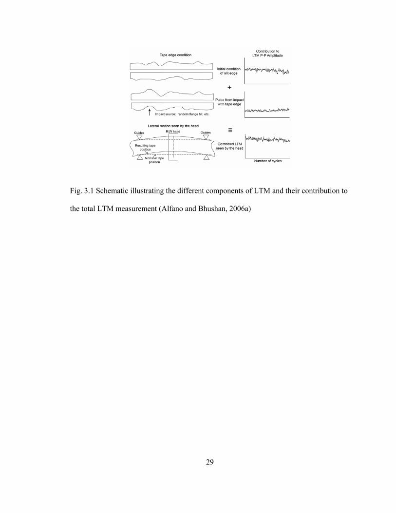
29
Fig. 3.1 Schematic illustrating the different components of LTM and their contribution to
the total LTM measurement (Alfano and Bhushan, 2006a)
30
the tape edge contour and the tape edge position are measured simultaneously (Goldade
and Bhushan, 2004; Hansen and Bhushan, 2004). By combining the tape edge defects
and repeatable tape movements, the true LTM is obscured by this noise, and it is
desirable to develop a method of measuring tape motion that does not incorporate edge
defects and repeatable motion. It is for this reason that a new method is developed with
the objective of measuring only the true LTM while rejecting these other sources of
LTM.
In this paper, a videographic method is developed and evaluated where a
reference mark on the tape is monitored with a video camera and post processed to
determine its position. By creating the reference mark on the tape in the drive, it closely
approximates a magnetic signal that has been written to the tape and is able to reject
repeatable motion and edge defect contributions. The reason that this method is able to
reject repeatable LTM is that the movement of the tape during writing, as measured with
an edge probe, will generally be of a repeatable nature. Since this tape motion is
repeatable, subsequent reading passes will see the data track as a nearly straight line,
although there may be significant LTM as measured by the edge probe.
3.2. Experimental Details
3.2.1. Description of tape transport and test procedure
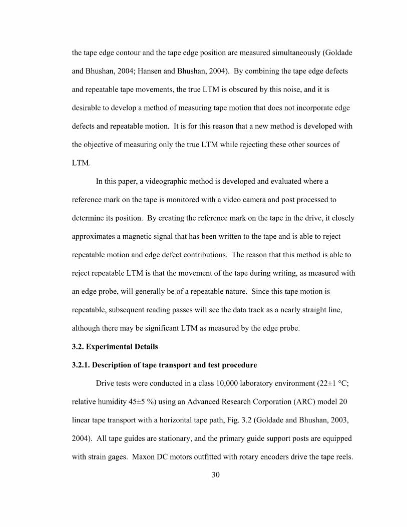
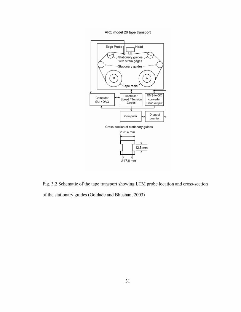
Drive tests were conducted in a class 10,000 laboratory environment (22±1 °C;
relative humidity 45±5 %) using an Advanced Research Corporation (ARC) model 20
linear tape transport with a horizontal tape path, Fig. 3.2 (Goldade and Bhushan, 2003,
2004). All tape guides are stationary, and the primary guide support posts are equipped
with strain gages. Maxon DC motors outfitted with rotary encoders drive the tape reels.
31
Fig. 3.2 Schematic of the tape transport showing LTM probe location and cross-section
of the stationary guides (Goldade and Bhushan, 2003)
32
Both reels must rotate in the same direction with the supply reel producing a slight
negative torque to maintain tape tension. Controller software calculates tape tension
from the measured deflection of the primary guides and the known wrap angles around
the guides. The controller software samples the rotary encoders every millisecond to
calculate the motor angular speed and maintains constant average tape tension throughout
the pass. Tape is loaded onto a reel until the diameter of the pack is 60 mm. Controller
software calculates tape linear velocity from reel angular velocity and original tape pack
diameter and maintains constant linear speed throughout the pass. The pass length was
set at 100 m for all tests, with one forward and reverse pass equal to one 200 m cycle.
Nominal speed and tension were 6 m/s and 0.5 N.
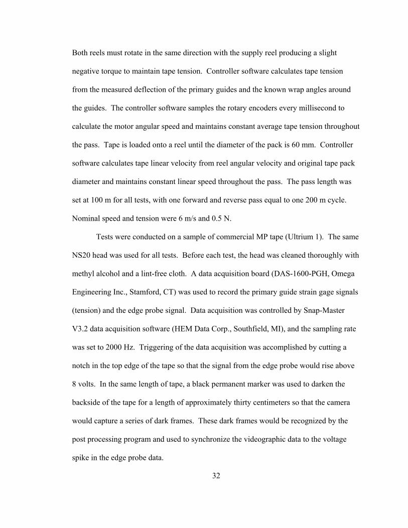
Tests were conducted on a sample of commercial MP tape (Ultrium 1). The same
NS20 head was used for all tests. Before each test, the head was cleaned thoroughly with
methyl alcohol and a lint-free cloth. A data acquisition board (DAS-1600-PGH, Omega
Engineering Inc., Stamford, CT) was used to record the primary guide strain gage signals
(tension) and the edge probe signal. Data acquisition was controlled by Snap-Master
V3.2 data acquisition software (HEM Data Corp., Southfield, MI), and the sampling rate
was set to 2000 Hz. Triggering of the data acquisition was accomplished by cutting a
notch in the top edge of the tape so that the signal from the edge probe would rise above
8 volts. In the same length of tape, a black permanent marker was used to darken the
backside of the tape for a length of approximately thirty centimeters so that the camera
would capture a series of dark frames. These dark frames would be recognized by the
post processing program and used to synchronize the videographic data to the voltage
spike in the edge probe data.
33
3.2.2. LTM measurement
3.2.2.1 Optical edge probe
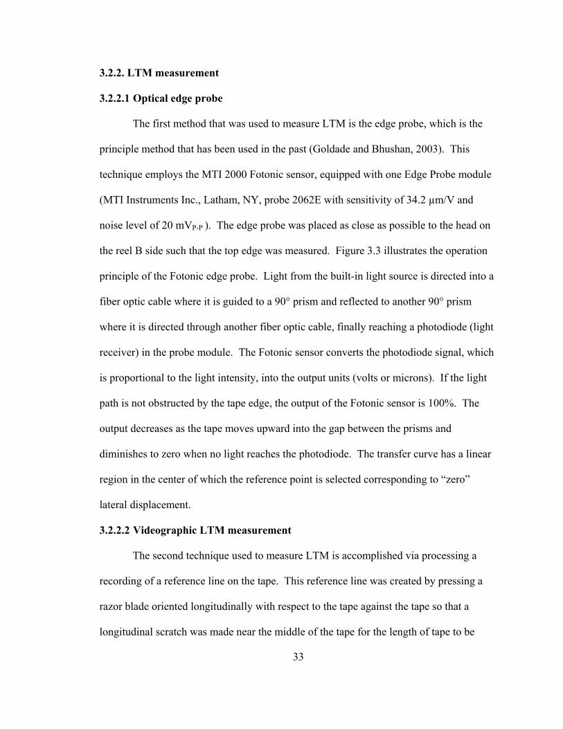
The first method that was used to measure LTM is the edge probe, which is the
principle method that has been used in the past (Goldade and Bhushan, 2003). This
technique employs the MTI 2000 Fotonic sensor, equipped with one Edge Probe module
(MTI Instruments Inc., Latham, NY, probe 2062E with sensitivity of 34.2 µm/V and
noise level of 20 mVP-P ). The edge probe was placed as close as possible to the head on
the reel B side such that the top edge was measured. Figure 3.3 illustrates the operation
principle of the Fotonic edge probe. Light from the built-in light source is directed into a
fiber optic cable where it is guided to a 90° prism and reflected to another 90° prism
where it is directed through another fiber optic cable, finally reaching a photodiode (light
receiver) in the probe module. The Fotonic sensor converts the photodiode signal, which
is proportional to the light intensity, into the output units (volts or microns). If the light
path is not obstructed by the tape edge, the output of the Fotonic sensor is 100%. The
output decreases as the tape moves upward into the gap between the prisms and
diminishes to zero when no light reaches the photodiode. The transfer curve has a linear
region in the center of which the reference point is selected corresponding to “zero”
lateral displacement.
3.2.2.2 Videographic LTM measurement
The second technique used to measure LTM is accomplished via processing a
recording of a reference line on the tape. This reference line was created by pressing a
razor blade oriented longitudinally with respect to the tape against the tape so that a
longitudinal scratch was made near the middle of the tape for the length of tape to be
34
Fig. 3.3 Schematic showing detail of the optical edge probe measurement technique
(Goldade and Bhushan, 2003)
35
monitored. Making a perfectly straight line is not the goal of this process; rather, it is to
create a reference line that mimics the behavior of a magnetic signal written where the
repeatable motion of the tape is effectively cancelled by creating a line that stays in the
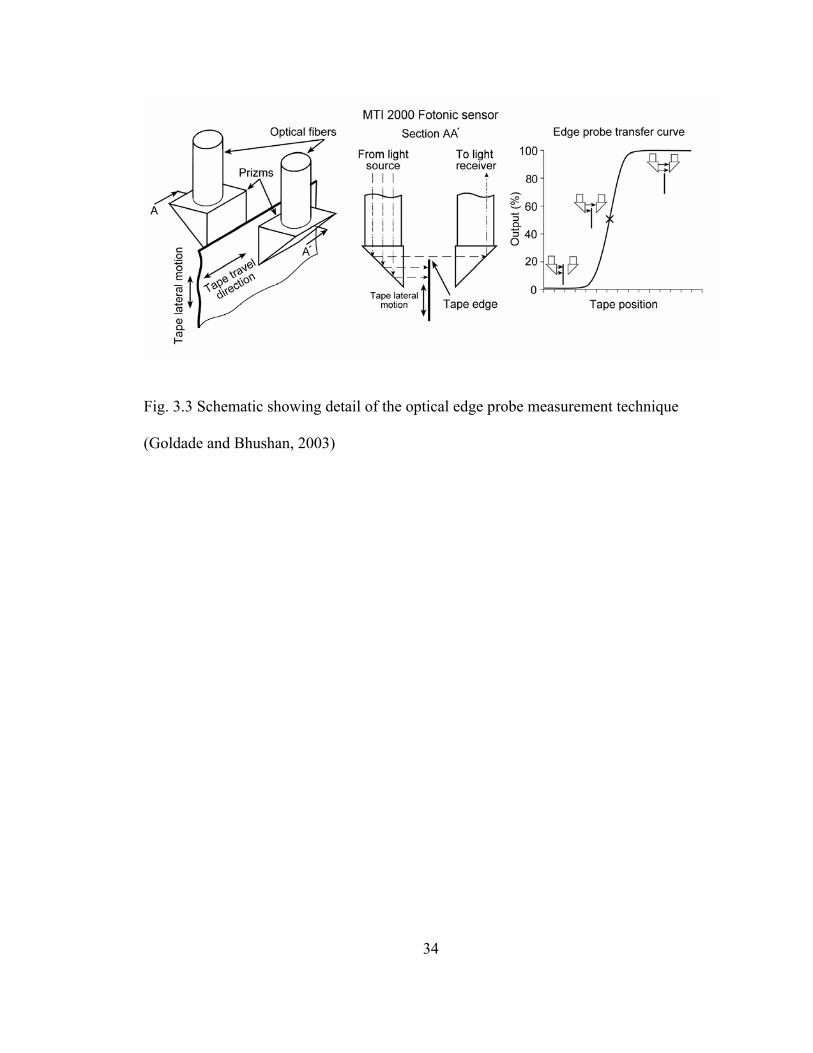
same position with respect to the head instead of the tape edges. Figure 3.4 illustrates
how the tape path was modified by adding a roller guide to allow an adequate amount of
room to position the razor blade and to back up the tape to minimize distortion. The
force applied to the razor blade was adjusted such that the backcoat was penetrated,
exposing the substrate. Even with these precautions, a ridge of 10 µm was created on the
front side of the tape. The width of this scratch is 16 µm with a standard deviation of 1.9
µm.
Once the tape has been marked, the guide and razor blade are removed in order to
provide the camera a clear view of the head. The camera used was a Lumenera 2-2
monochrome camera (Lumenera Corporation, Ottawa, Ontario, Canada) with a pixel size
of 4.4 µm square. A Nikon 105mm f/2D AF DC-Nikkor (Nikon Corporation, Tokyo,
Japan) lens was used by fitting it with a C-mount lens adapter. The region of interest for
the camera was created as a small rectangle centered vertically on the scratch with the
short side parallel to the longitudinal direction in order to increase the frame rate from 12
frames per second to 86±1 frames per second. The camera created a single file that
contained all 100 cycles of each test which was broken into individual cycles during post
processing.
3.2.2.3 LTM analysis
Taylor and Talke (2005) report that for frequencies above 1000 Hz, LTM must be
reduced to below 100 nm P-P for an open loop condition in order to prevent read/write
36
Fig. 3.4 Comparison of standard and scratching tape paths showing camera location in
relation to the tape deck
37
errors since the servo systems are not able to accommodate motion in this frequency
range. Below 1000 Hz, servo systems are able to accommodate most LTM events.
Exceptions to this are that if the LTM event is of great enough magnitude or acceleration,
it exceeds the mechanical capabilities of the servo system, even below 1000 Hz, resulting
in TMR or loss of servo lock. Since magnitude of LTM is, arguably, the most important
factor, LTM mean total amplitude (ATM) is used as the measurement for tape motion
measurements.
Physical LTM mean total amplitude (LTMP ATM) was calculated by dividing the
pass into four equal sections of approximately 20 m and finding the average difference
between the highest and lowest value for the four sections. LTMP ATM is a slight
modification to the Rz (DIN 4768) standard where the number of measurement regions
was changed from five to four due to limitations of the data acquisition/analysis software.
This particular measurement was chosen because it is able to indicate persistent extreme
values of LTM but is less sensitive to unusually large LTM anomalies than a direct peak-
to-peak measurement for the entire pass (Wright and Bhushan, 2006). To calculate
LTMP ATM, the initial and final 10 m were neglected in order to ensure that the drive was
operating at steady state while the measurements were taken. Next, the range (maximum
minus the minimum) for each of these four sections is determined. Finally, the four
ranges are averaged to yield the final LTMP ATM value. LTM is also presented in power
spectrum density (PSD) plots so that a comparison of the frequency components may be
compared. PSD is calculated using Matlab version 7.0.1 Service Pack 1 from The
Mathworks, Inc. A program was written to parse the LTM data into one-second blocks,
to fast Fourier transform each block, and to perform scaling to obtain the power
38
contained at interval frequencies for the entire cycle. The resulting PSD plot was very
repeatable; as a result, only one representative plot is shown.
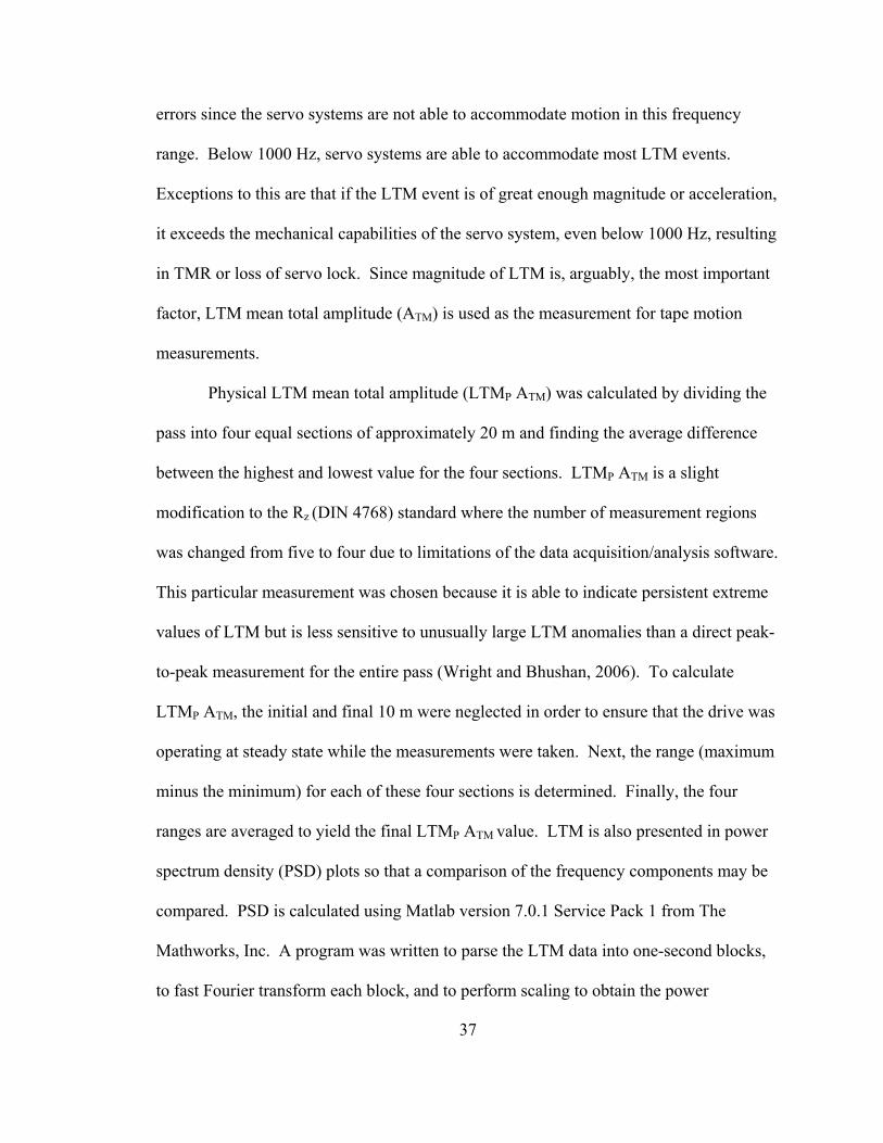
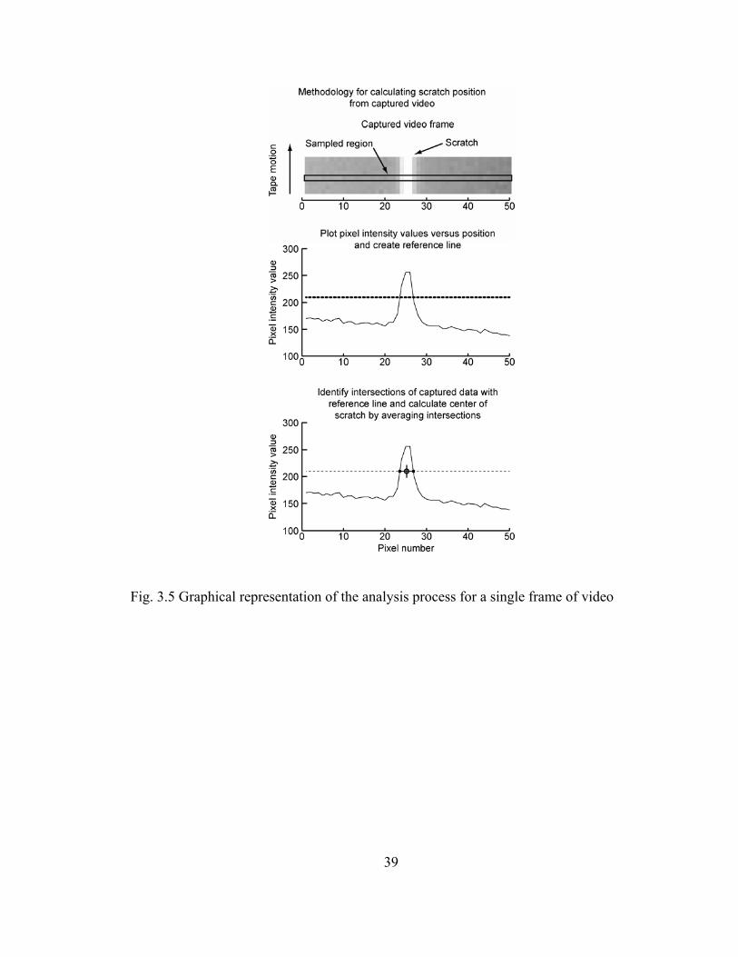
Videographic LTM mean total amplitude (LTMV ATM amplitude) was calculated
using another Matlab program. This program would first import the video data and
inspect a single row of pixels in each individual frame. Next, it identified where to begin
analysis by finding “dark” frames at the beginning of each pass where the tape had been
covered in permanent marker. Once the beginning of the tape was detected, the program
located the scratch edges by creating a reference value which was the mean value for the
frame plus thirty percent and interpolating where the adjacent pixel values crossed this
threshold. After the edges were located, they were averaged, and this value is the tape
position. Figure 3.5 shows this process as it would appear if it were done graphically.
After the tape position is calculated for every frame of interest for each pass, it is treated
the same as the optical edge probe data. Specifically, it is broken up into four equal
length time segments. The range is found for each of these sections and then these four
ranges are averaged to yield the ATM value for the pass.
3.3. Results and discussion
LTM was measured using a new technique that reports a more accurate value of
the true LTM, and the results of this method are presented alongside those of the optical
edge probe. As the results from all tests are similar, only one test is presented here on
behalf of the others.
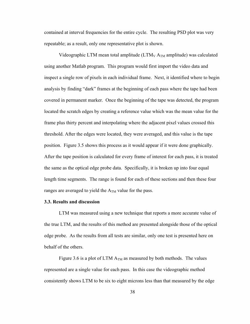
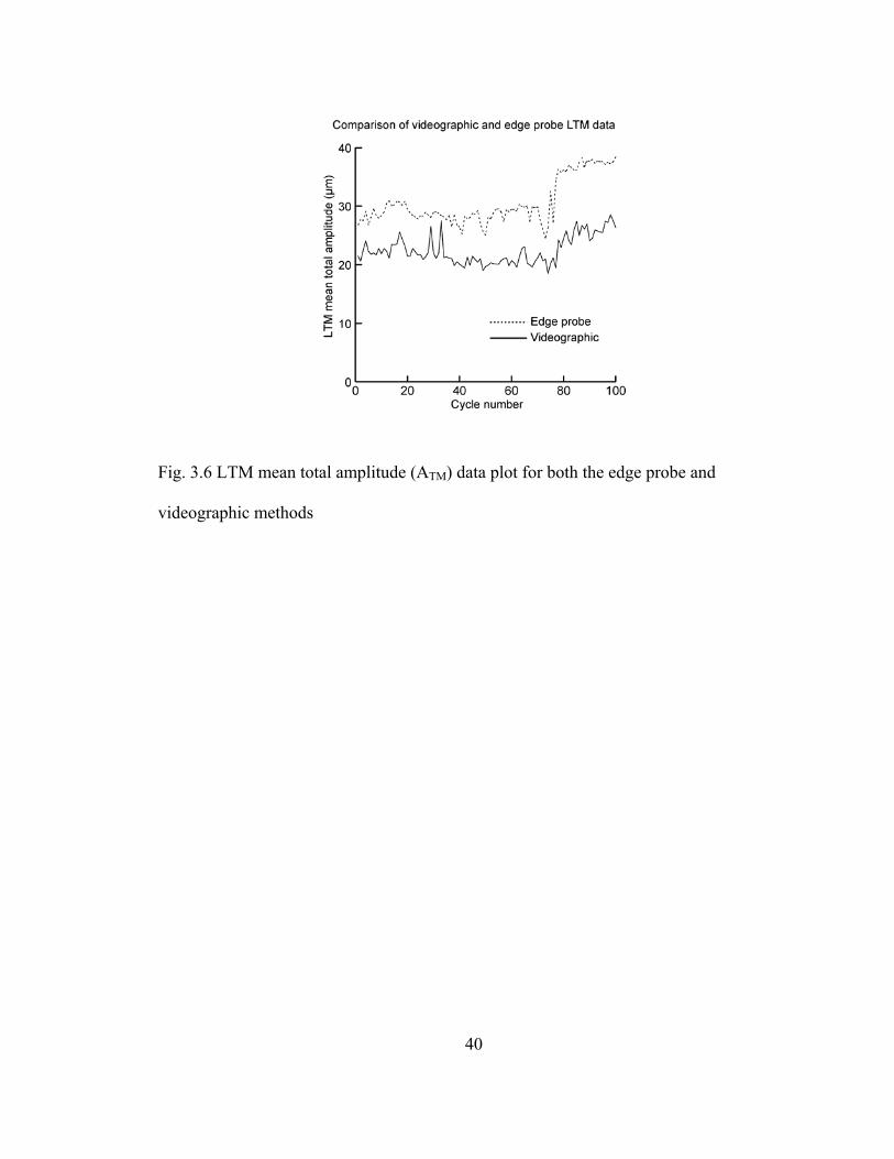
Figure 3.6 is a plot of LTM ATM as measured by both methods. The values
represented are a single value for each pass. In this case the videographic method
consistently shows LTM to be six to eight microns less than that measured by the edge
39
Fig. 3.5 Graphical representation of the analysis process for a single frame of video
40
Fig. 3.6 LTM mean total amplitude (ATM) data plot for both the edge probe and
videographic methods
41
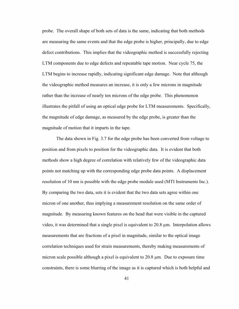
probe. The overall shape of both sets of data is the same, indicating that both methods
are measuring the same events and that the edge probe is higher, principally, due to edge
defect contributions. This implies that the videographic method is successfully rejecting
LTM components due to edge defects and repeatable tape motion. Near cycle 75, the
LTM begins to increase rapidly, indicating significant edge damage. Note that although
the videographic method measures an increase, it is only a few microns in magnitude
rather than the increase of nearly ten microns of the edge probe. This phenomenon
illustrates the pitfall of using an optical edge probe for LTM measurements. Specifically,
the magnitude of edge damage, as measured by the edge probe, is greater than the
magnitude of motion that it imparts in the tape.
The data shown in Fig. 3.7 for the edge probe has been converted from voltage to
position and from pixels to position for the videographic data. It is evident that both
methods show a high degree of correlation with relatively few of the videographic data
points not matching up with the corresponding edge probe data points. A displacement
resolution of 10 nm is possible with the edge probe module used (MTI Instruments Inc.).
By comparing the two data, sets it is evident that the two data sets agree within one
micron of one another, thus implying a measurement resolution on the same order of
magnitude. By measuring known features on the head that were visible in the captured
video, it was determined that a single pixel is equivalent to 20.8 µm. Interpolation allows
measurements that are fractions of a pixel in magnitude, similar to the optical image
correlation techniques used for strain measurements, thereby making measurements of
micron scale possible although a pixel is equivalent to 20.8 µm. Due to exposure time
constraints, there is some blurring of the image as it is captured which is both helpful and
42
Fig. 3.7 Real-time plot of data from the edge probe and videographic methods
43
harmful. It is helpful for the post processing in that it evens out the texture of the
background but detrimental in that it creates a certain degree of uncertainty which is
reflected in the resolution capabilities. As expected, but unavoidable due to limitations of
readily available equipment, the sampling rate of 86 Hz for the videographic method is
insufficient, resulting in peaks being missed by the videographic method that the edge
probe method does not. It is expected that this frequency limitation does not significantly
impact the mean total amplitude values reported above. Most of the peaks are indeed
measured by the videographic method and a more erratic trace would be expected for the
videographic method in Fig. 3.6 due to large ATM measurements being made in some
cycles but not in others.
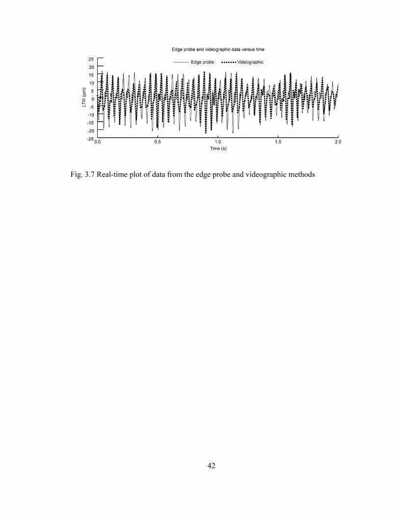
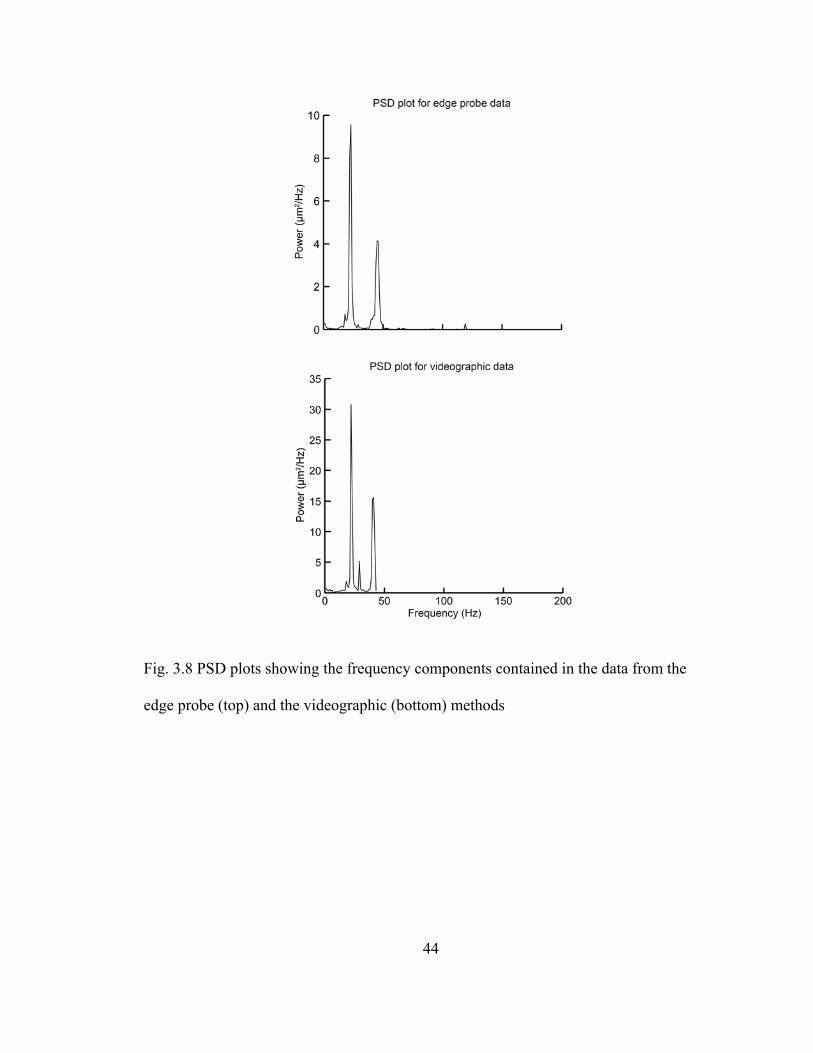
Frequency spectrum analysis yields the plots shown in Fig. 3.8. Here the
frequency components are calculated using a fast Fourier transform. Both sets of data
have nearly identical frequency components up to 43 Hz since this is the maximum
frequency that can be analyzed with the videographic method. The second largest peak
for the videographic method is shifted to the left slightly, but this area is somewhat
inaccurate since it is so close to the Nyquist frequency, so some error is expected. After
the data presented in Fig. 3.7, this information should not be surprising since both sets of
data have similar compositions and would therefore have similar frequency components.
3.4. Conclusions
This study has determined that it is possible to calculate tape position using a
video camera with similar accuracy to that of an optical edge probe. It has been shown
that the edge probe combines the effect of the tape edge and the true LTM of the tape
resulting in a exaggerated measure of LTM, but this new method allows for a reference
44
Fig. 3.8 PSD plots showing the frequency components contained in the data from the
edge probe (top) and the videographic (bottom) methods
45
line to be made in the system, thereby approximating a magnetic signal written to the tape
and eliminating effects of the tape edge. Important observations made in this study are
summarized below.
• Results of the videographic method show a true LTM that is six to eight microns less
than those reported by the edge probe, indicating that this method is capable of
rejecting edge defect and repeatable tape motion contributions. This is the expected
result and shows the same trend as what has been previously presented (Alfano and
Bhushan, 2006a).
• The correlation between the two methods is a very good indication that the
videographic method has the resolution necessary to be used for this type of
measurement. As mentioned previously, the major limitation to this method in the
current iteration is that its sampling rate is only 86 Hz and a sampling rate of at least
1000 Hz is desirable.
There are a couple of modifications that could improve this method in the future.
First, the largest gains in performance would be obtained by using a line scan camera.
This type of camera provides a similar resolution to what is available here but is able to
operate at much higher sampling rates, 1000’s of Hz. Although this type of camera only
produces a single row of pixels, that is all that was used in the analysis for this study.
The second area where improvements can be made is the method used to mark the tape.
This method produced less distortion of the tape than other methods that were attempted
and did not have any obvious adverse effects since both optical probe LTM values and
frequency components agree with previous work (Hansen and Bhushan, 2004), but any

46
distortion in the tape may affect LTM results and should be avoided where possible.
Therefore, it is of interest to develop a method that has as little effect on the physical
characteristics of the tape as possible.
47
CHAPTER 4
VIBRATION ANALYSIS OF AXIALLY MOVING MAGNETIC TAPE WITH COMPARISONS TO STATIC AND DYNAMIC EXPERIMENTAL RESULTS
4.1. Motivation
Capacities of magnetic tape are currently 400 GB (800 GB compressed) for LTO
Ultrium 3 and 500 GB (1.3 TB compressed) for SAIT (Anonymous, 2004, 2005). In
order to create a multi-terabyte capacity, cartridge manufacturers are increasing the areal
data density as well as the volumetric density (Bhushan, 1996, 2000). Increasing the
areal density results in higher capacity for a given volume of tape by decreasing both the
track pitch and the length of a bit. By using a thinner substrate and coatings, a greater
length of tape can be wound on a cartridge, thereby increasing data capacity for a given
volume.
As the areal density increases, the head-to-tape spacing must decrease in order to
maintain an acceptable signal-to-noise ratio and resolution (Bhushan, 1996). This
requires the tape to be smoother to minimize the asperity-induced head-to-tape spacing.
A side effect of having a smooth tape is that the coefficient of friction increases due to a
higher real area of contact and greater compliance (Bhushan, 2000). To reduce the
effects of the increased coefficient of friction, the tension is reduced, but this has the
negative effect of increasing the flying height of the tape over the heads and guides since
48
the hydrodynamic forces are affected to a lesser degree by the thickness of the substrate
(Elrod and Eshel, 1965). Potentially, the tape path becomes less stable and lateral tape
motion (LTM) becomes greater as the flying height increases due to reduced frictional
forces that would otherwise dampen the motion. This is a problem because if LTM
becomes excessive, the data track will move away from the read/write elements of the
head causing a track misregistration (TMR). In practice, the probability of TMR is
reduced in a commercial drive with a servo mechanism that follows a servo track written
at the time of manufacture and reduces the effect an LTM event has on data retrieval.
These tracking mechanisms have a limited bandwidth, typically less than 1 kHz, and
TMR may still occur if the LTM event is of significant amplitude and accelerates faster
than the servo mechanism can track it (Richards and Sharrock, 1998). The track widths
in next generation data patterns are narrower, which means that they have even less
tolerance of LTM before TMR occurs (Richards and Sharrock, 1998; Goldade and
Bhushan, 2003; Wang et al., 2003). Tape guiding that minimizes LTM is desirable and
as Goldade and Bhushan (2003) suggested, tape guiding is dependent on the quality of
the virgin tape edge, tape tension and speed, and type of guiding (stationary/rotary,
active/passive), among other factors.
In a previous study, a vibration model was developed to study the response of a
tape when subjected to a reel tilt input with tape guide impacts (Boyle and Bhushan,
2006). This previous study modeled the system as a stationary fixed-fixed Euler-
Bernoulli beam with consideration of guide impacts. The current study implements a
mathematical model to predict the natural frequencies and mode shapes for a tape
undergoing axial motion as operating parameters are varied and then compares this data
49
to experimental data and previous work. Accounting for the axial motion of the tape, the
system becomes a gyroscopic system. The parameters studied were axial velocity,
tension, free span length, and tape thickness as they relate to past, present, and future tape
drives. The beam is modeled as an axially moving Euler-Bernoulli beam with lateral
vibration being the subject of investigation. By knowing the effect of varying these
parameters, future drive can be designed to minimize sources of excitation which match
those of the tape. In this model the effects of wrapping around the guides and head,
damping at the guides and head, impacts with the tape edge, effects of tape cupping, and
air entrainment at the reels are neglected so that the simplest possible model with axial
velocity may be studied.
4.2. Sources of LTM
There are several sources of LTM in a tape drive. The drive reels, rotary guides,
tape pack, and tape edge all contribute to the excitation of the system. Tilting of the
reels, as if they had been placed on a bent axle, results in a periodic lateral motion being
imparted on the tape as illustrated in Fig. 4.1(a). Sources of this tilt include the entire reel
being skewed, hub imperfections, and misaligned/damaged flanges. Since the tilt is fixed
to the rotational position of the reel, it excites the tape at the reel rotational frequency.
Rotary guides also induce vibrations in much the same way as the reels but are generally
smaller in diameter and therefore rotate with a higher frequency. If the guides are tilted,
there may be periodic contacts with the flanges of the guides, causing an impact and
exciting the tape.
Imperfections in the tape pack and edge also contribute to LTM in the following
ways. During winding, wraps of tape will slide due to air being trapped between the
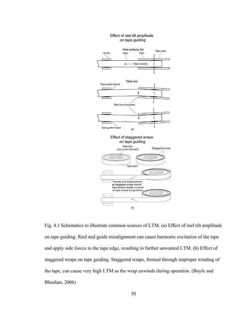
50
Fig. 4.1 Schematics to illustrate common sources of LTM. (a) Effect of reel tilt amplitude
on tape guiding. Reel and guide misalignment can cause harmonic excitation of the tape
and apply side forces to the tape edge, resulting in further unwanted LTM. (b) Effect of
staggered wraps on tape guiding. Staggered wraps, formed through improper winding of
the tape, can cause very high LTM as the wrap unwinds during operation. (Boyle and
Bhushan, 2006)
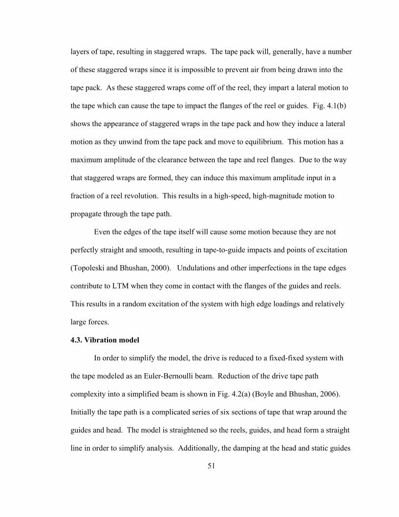
51
layers of tape, resulting in staggered wraps. The tape pack will, generally, have a number
of these staggered wraps since it is impossible to prevent air from being drawn into the
tape pack. As these staggered wraps come off of the reel, they impart a lateral motion to
the tape which can cause the tape to impact the flanges of the reel or guides. Fig. 4.1(b)
shows the appearance of staggered wraps in the tape pack and how they induce a lateral
motion as they unwind from the tape pack and move to equilibrium. This motion has a
maximum amplitude of the clearance between the tape and reel flanges. Due to the way
that staggered wraps are formed, they can induce this maximum amplitude input in a
fraction of a reel revolution. This results in a high-speed, high-magnitude motion to
propagate through the tape path.
Even the edges of the tape itself will cause some motion because they are not
perfectly straight and smooth, resulting in tape-to-guide impacts and points of excitation
(Topoleski and Bhushan, 2000). Undulations and other imperfections in the tape edges
contribute to LTM when they come in contact with the flanges of the guides and reels.
This results in a random excitation of the system with high edge loadings and relatively
large forces.
4.3. Vibration model
In order to simplify the model, the drive is reduced to a fixed-fixed system with
the tape modeled as an Euler-Bernoulli beam. Reduction of the drive tape path
complexity into a simplified beam is shown in Fig. 4.2(a) (Boyle and Bhushan, 2006).
Initially the tape path is a complicated series of six sections of tape that wrap around the
guides and head. The model is straightened so the reels, guides, and head form a straight
line in order to simplify analysis. Additionally, the damping at the head and static guides
52
is not taken into account because, at speed, the tape “flies” over these elements once a
hydrodynamic bearing is formed. This hydrodynamic effect is less likely in smooth roller
bearings and unlikely in those with air bleed channels where there will generally be tape-
to-guide contact, although these forces are neglected as well for simplification. Once the
tape path is straightened, the various components of the tape path are replaced by a
schematic representation of how they affect the tape path. The reels are effectively a
fixed constraint, and the guide flanges are modeled as point contacts with a clearance
between the tape and flange. The final simplification is made in Fig. 4.2(b) where the
guides and head are removed completely to create the maximum free span so that the
natural frequencies of the system are unaffected by additional forces.
The equation of motion for an Euler-Bernoulli beam with axial velocity V for this
system is (Chubachi, 1958; Mote, 1965)
( )LXFXUEI
XUP
XUV
TXUV
TU ,0 ,
2 4
4
2
2
2
22
2
2
2
∈=∂∂
+∂∂
−
∂∂
+∂∂
∂+
∂∂ρ , (1)
where ( )TXU , is the transverse displacement, ρ is the linear density, P is the tension, E
is the modulus of elasticity, I is the moment of inertia, and F is the external force. The
following variables are used to nondimensionalize the system
EIFLfEIPL
EIVLvLEITtLUuLXx322
4
,
, , , ,
==
====
µ
ρρ. (2)
Substituting the variables of Eq. 2 into Eq. 1 yields
( )2 22 , 0,1tt xt xx xx xxxxu vu v u u u f xµ+ − − + = ∈ (3)
where the subscripts indicate differentiation. Here the method of Wickert and Mote
(1990) is used to complete the modal analysis. Using the following differential operators
53
Fig. 4.2 (a) Reduction of the tape path to a schematic representation of the system (b)
Final simplification into a fixed-fixed Euler-Bernoulli beam model with axial velocity V.
54
( ) 4
4
2
222 ,2 ,~
xxvK
xvGIM
∂∂
+∂∂
−−=∂∂
== µ, (4)
where I~ is the identity operator, Eq. 3 can be rewritten as the second order equation
fKuGuMu ttt =++ (5)
M is the mass operator, G is the gyroscopic operator, and K is the stiffness operator. The
equation of motion (Eq. 3) can be cast in first order form as
qBwAw =+t (6)
where the state and excitation vectors are
( )
=
=0
),( ,f
txuu
tx t qw (7)
and the matrix differential operators are
=
=
0K-KG
0
0BA
KM
(8)
where A is symmetric and B is skew symmetric. Equation 6 must satisfy the initial
conditions
==)()(
)0,(xaxb
txw (9)
and the following boundary conditions
0)0,1()0,1(0)0,0()0,0(
============
txtxtxtx
x
x
wwww
(10)
Systems that have a symmetric and skew symmetric matrix are gyroscopic. Physically, it
is the Coriolis acceleration, G, that produces the gyroscopic properties. The Coriolis
acceleration is a function of the axial velocity, and as the axial velocity increases, so does

55
the force due to the Coriolis acceleration. At some axial velocity, the gyroscopic forces
overcome the restoring force. This axial velocity is called the critical velocity and is
defined as
22 4πµ +=cv , (11)
for an axially moving beam with fixed-fixed boundary conditions (Wickert and Mote,
1990).
4.3.1. Natural frequency analysis
The general and separable solution to Eq. 6 is
{ }( , ) Re ( ) tx t x eλφ=w (12)
where the eigenvalues are imaginary n niλ ω= and the eigenvectors φn are complex.
Equation 12 leads to the eigenvalue problem
0λ + =A Bφ φ . (13)
Solution of the eigenvalue problem results in the eigenfunctions being a linear
combination of i xce γ , with nontrivial solutions that satisfy the dispersion relation
(Wickert and Mote, 1990)
( ) 02 22224 =++−+ λλγγµγ ivv . (14)
Additionally, the boundary conditions (10) require that the four roots γk of (14) are related
by
( ) ( ) ( ) ( )( ) ( ) ( ) ( ) ( )( )( ) ( ) ( ) ( )( )
3 4 2 31 2 1 4
1 3 2 4
1 2 4 3 2 3 4 1
1 3 2 4
0
i ii i
i i
e e e e
e e
γ γ γ γγ γ γ γ
γ γ γ γ
γ γ γ γ γ γ γ γ
γ γ γ γ
+ ++ +
+ +
− − + + − − +
+ − − + = (15)
A Matlab program was developed to find values of λ. It accomplished this task by starting
at a value for ω slightly above zero and substituting this value into Eq. 14, at which point
56
the roots γk of Eq. 14 were calculated. Next, the roots of Eq. 14 are substituted into Eq.
15. The result of Eq. 15 approaches zero when the roots of Eq. 14 are those of a natural
frequency. The program takes advantage of the fact that the absolute value of Eq. 15
versus ω, where ω is the frequency used to calculate the roots of Eq. 14, is similar in
shape to the absolute value of the sine function in that it is smooth and continuous
between zeros where cusps are found. The program successively increases the value of ω
until the absolute value of Eq. 15 for ωm, where m is the index, was less than the absolute
value of Eq. 15 for ωm+1. Once this condition is satisfied, the value of ωm-1 is used as a
starting value, the step size is reduced by an order of magnitude, and iteration resumes by
increasing the value of ω by this new step size. This process was repeated until the
specified resolution was reached, and ωm was stored as ωn, the nth natural frequency. At
this point, the step size would be reset to the initial value and the iterations would resume
with the initial value of ωm being set to ωm+1 in order to calculate the next natural
frequency. This process was repeated until the specified number of natural frequencies
had been determined. In principle, the program finds the local minima of the functions
numerically through iteration.
4.3.2. Modal analysis
Once the natural frequencies had been determined, the roots of Eq. 14 for ωn are
summed to determine the eigenfunction for the mode shape
( ) ∑=
=4
1k
xik
kecx γψ . (16)
57
The final step in determining the mode shape is the determination of the values for each
ck. The boundary conditions (Eq. 10) are applied to Eq. 16 resulting in a set of four
homogeneous algebraic equations that can be written in matrix form as
0=Ac (17)
where { }1 2 3 4Tc c c c=c is the coefficient vector and A is the matrix of coefficients
(Gaith, M. and Muftu, S., 2005). Since the coefficient matrix is singular, not all values of
c can be calculated. A common method of solution is to solve for each coefficient such
that they are all in terms of a single coefficient such as c1. (c1) becomes (c1)n and is the
arbitrary constant of the eigenfunction which depends on n (Inman, 2001).
4.4. Experimental details
4.4.1. Description of the dynamic test apparatus and test procedure
Drive tests were conducted in a class 10,000 laboratory environment (22±1 °C;
relative humidity 45±5 %) using an Advanced Research Corporation (ARC) model 20
linear tape transport with a horizontal tape path and stationary guides. A detailed
description of the drive components and drive operation have been presented previously
(Goldade and Bhushan, 2003; Hansen and Bhushan, 2004). A series of tests for 6.5 µm
metal particle (MP) tape were run according to Table 4.1. The tape was tested at every
combination of tension and axial velocity for a total of nine tests. Each test had a pass
length of 100 m and was monitored for ten cycles.
Axial velocity (m/s) Tension (N) 4 0.5 6 1.0 8 1.5
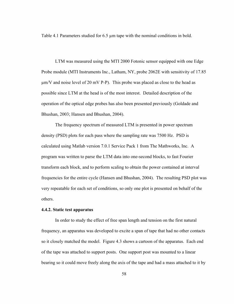
58
Table 4.1 Parameters studied for 6.5 µm tape with the nominal conditions in bold.
LTM was measured using the MTI 2000 Fotonic sensor equipped with one Edge
Probe module (MTI Instruments Inc., Latham, NY, probe 2062E with sensitivity of 17.85
µm/V and noise level of 20 mV P-P). This probe was placed as close to the head as
possible since LTM at the head is of the most interest. Detailed description of the
operation of the optical edge probes has also been presented previously (Goldade and
Bhushan, 2003; Hansen and Bhushan, 2004).
The frequency spectrum of measured LTM is presented in power spectrum
density (PSD) plots for each pass where the sampling rate was 7500 Hz. PSD is
calculated using Matlab version 7.0.1 Service Pack 1 from The Mathworks, Inc. A
program was written to parse the LTM data into one-second blocks, to fast Fourier
transform each block, and to perform scaling to obtain the power contained at interval
frequencies for the entire cycle (Hansen and Bhushan, 2004). The resulting PSD plot was
very repeatable for each set of conditions, so only one plot is presented on behalf of the
others.
4.4.2. Static test apparatus
In order to study the effect of free span length and tension on the first natural
frequency, an apparatus was developed to excite a span of tape that had no other contacts
so it closely matched the model. Figure 4.3 shows a cartoon of the apparatus. Each end
of the tape was attached to support posts. One support post was mounted to a linear
bearing so it could move freely along the axis of the tape and had a mass attached to it by

59
Fig. 4.3 The static test apparatus used to study the effects of free span length, tape
thickness, and tension of the first natural frequency by directly exciting the tape.
60
a string which was then hung over a bearing in order to provide tension to the tape. The
other support was attached to a vertically oriented loudspeaker driver and was reinforced
to prevent the tension from tilting the support post. Measurements were made at the mid
point of the free span and also at the excited end of the tape by using the MTI 2000
Fotonic sensor equipped with two Edge Probe modules (sensitivity of 17.85 µm/V and
noise level of 20 mVP-P and a second probe with a sensitivity of 14.72 µm/V). The mid
span peak-to-peak (P-P) amplitude was divided by the P-P amplitude of the excitation to
determine the amplitude ratio in order to correct for any nonlinearities of the amplifier
and loudspeaker driver system. A signal generator was used to produce a sinusoidal
signal which was then amplified by an audio amplifier that powered the loudspeaker
driver.
Tests were conducted by selecting a frequency and recording the P-P value
reported by the edge probes for each measurement location. P-P values were recorded at
1 Hz intervals for 0.5 m tests and 0.1 Hz intervals for 1.0 m tests in areas where the signal
changed quickly. Where the signal was changing more slowly, the data points varied
from 2 Hz to 5 Hz and 0.2 Hz to 0.5 Hz for 0.5 m and 1.0 m spans, respectively. Tests
were conducted for each thickness of tape at tensions of 0.5 N, 1.0 N, and 1.5 N for free
spans of 0.5 m and 1.0 m.
4.5. Results and discussion
4.5.1. Simulation
4.5.1.1 Natural frequency analysis
A program was written in Matlab to carry out the analysis described earlier
according to Table 4.2. These values are based on a combination of representative values
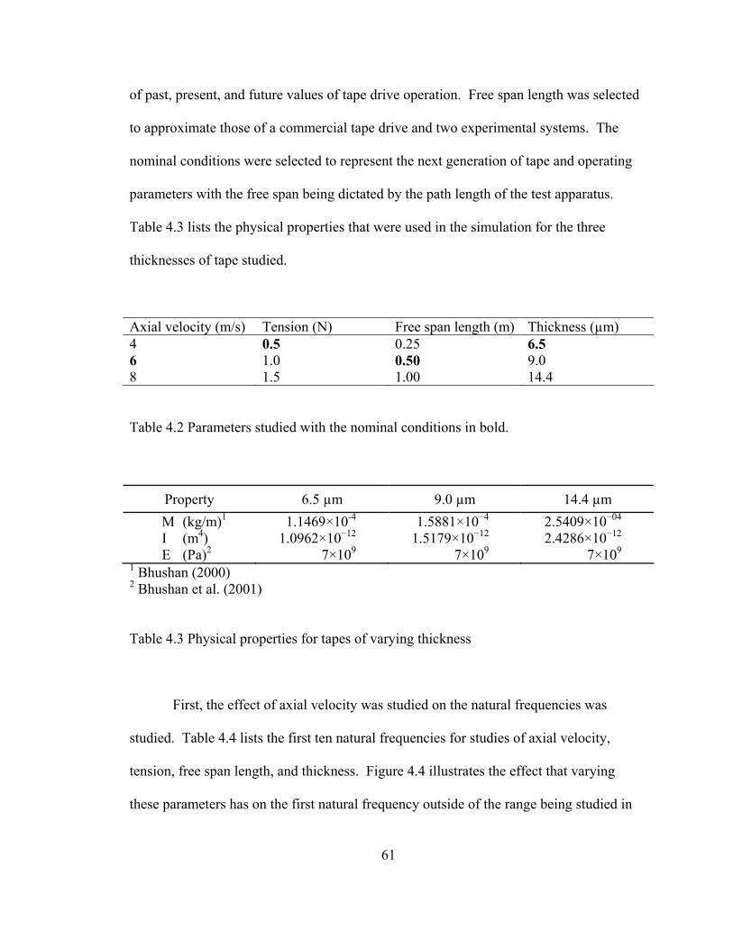
61
of past, present, and future values of tape drive operation. Free span length was selected
to approximate those of a commercial tape drive and two experimental systems. The
nominal conditions were selected to represent the next generation of tape and operating
parameters with the free span being dictated by the path length of the test apparatus.
Table 4.3 lists the physical properties that were used in the simulation for the three
thicknesses of tape studied.
Axial velocity (m/s) Tension (N) Free span length (m) Thickness (µm) 4 0.5 0.25 6.5 6 1.0 0.50 9.0 8 1.5 1.00 14.4 Table 4.2 Parameters studied with the nominal conditions in bold.
Property 6.5 µm 9.0 µm 14.4 µm M (kg/m)1 1.1469×10⁻⁴ 1.5881×10⁻⁴ 2.5409×10−04 I (m4) 1.0962×10⁻¹² 1.5179×10⁻¹² 2.4286×10⁻¹² E (Pa)2 7×10⁹ 7×10⁹ 7×10⁹ 1 Bhushan (2000) 2 Bhushan et al. (2001) Table 4.3 Physical properties for tapes of varying thickness
First, the effect of axial velocity was studied on the natural frequencies was
studied. Table 4.4 lists the first ten natural frequencies for studies of axial velocity,
tension, free span length, and thickness. Figure 4.4 illustrates the effect that varying
these parameters has on the first natural frequency outside of the range being studied in
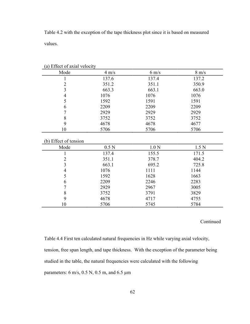
62
Table 4.2 with the exception of the tape thickness plot since it is based on measured
values.
(a) Effect of axial velocity Mode 4 m/s 6 m/s 8 m/s
1 137.6 137.4 137.2 2 351.2 351.1 350.9 3 663.3 663.1 663.0 4 1076 1076 1076 5 1592 1591 1591 6 2209 2209 2209 7 2929 2929 2929 8 3752 3752 3752 9 4678 4678 4677 10 5706 5706 5706 (b) Effect of tension
Mode 0.5 N 1.0 N 1.5 N 1 137.4 155.5 171.5 2 351.1 378.7 404.2 3 663.1 695.2 725.8 4 1076 1111 1144 5 1592 1628 1663 6 2209 2246 2283 7 2929 2967 3005 8 3752 3791 3829 9 4678 4717 4755 10 5706 5745 5784
Continued
Table 4.4 First ten calculated natural frequencies in Hz while varying axial velocity,
tension, free span length, and tape thickness. With the exception of the parameter being
studied in the table, the natural frequencies were calculated with the following
parameters: 6 m/s, 0.5 N, 0.5 m, and 6.5 µm
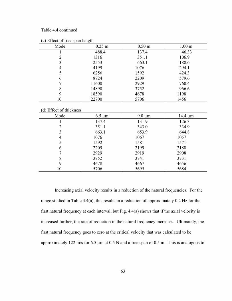
63
Table 4.4 continued (c) Effect of free span length
Mode 0.25 m 0.50 m 1.00 m 1 488.4 137.4 46.33 2 1316 351.1 106.9 3 2553 663.1 188.6 4 4199 1076 294.1 5 6256 1592 424.3 6 8724 2209 579.6 7 11600 2929 760.4 8 14890 3752 966.6 9 18590 4678 1198 10 22700 5706 1456 (d) Effect of thickness
Mode 6.5 µm 9.0 µm 14.4 µm 1 137.4 131.9 126.3 2 351.1 343.0 334.9 3 663.1 653.9 644.8 4 1076 1067 1057 5 1592 1581 1571 6 2209 2199 2188 7 2929 2919 2908 8 3752 3741 3731 9 4678 4667 4656 10 5706 5695 5684
Increasing axial velocity results in a reduction of the natural frequencies. For the
range studied in Table 4.4(a), this results in a reduction of approximately 0.2 Hz for the
first natural frequency at each interval, but Fig. 4.4(a) shows that if the axial velocity is
increased further, the rate of reduction in the natural frequency increases. Ultimately, the
first natural frequency goes to zero at the critical velocity that was calculated to be
approximately 122 m/s for 6.5 µm at 0.5 N and a free span of 0.5 m. This is analogous to
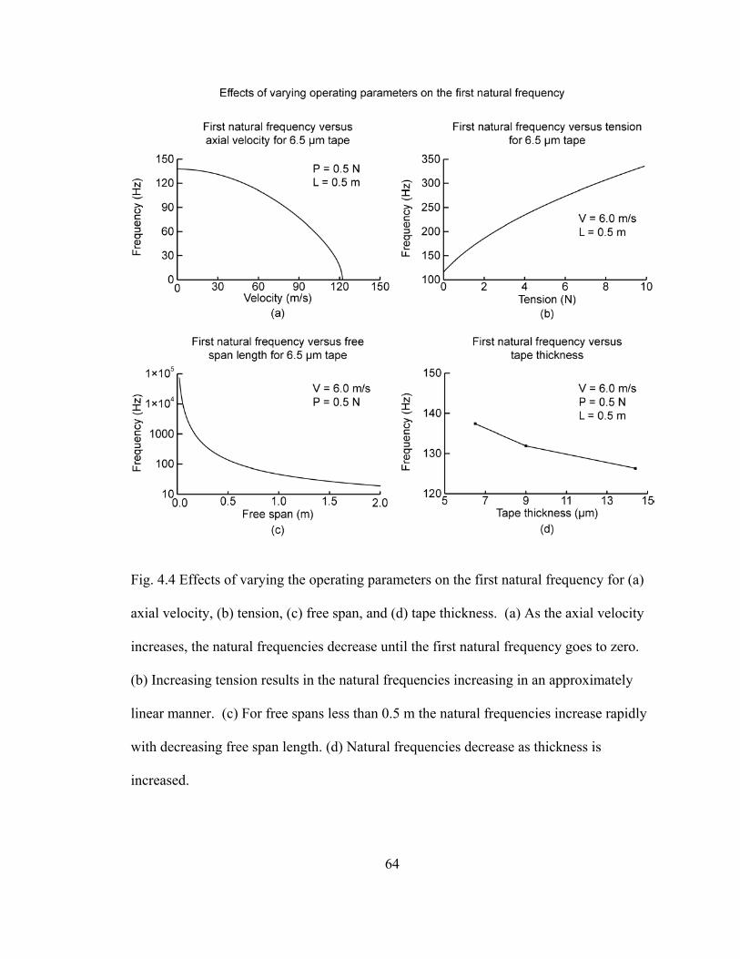
64
Fig. 4.4 Effects of varying the operating parameters on the first natural frequency for (a)
axial velocity, (b) tension, (c) free span, and (d) tape thickness. (a) As the axial velocity
increases, the natural frequencies decrease until the first natural frequency goes to zero.
(b) Increasing tension results in the natural frequencies increasing in an approximately
linear manner. (c) For free spans less than 0.5 m the natural frequencies increase rapidly
with decreasing free span length. (d) Natural frequencies decrease as thickness is
increased.
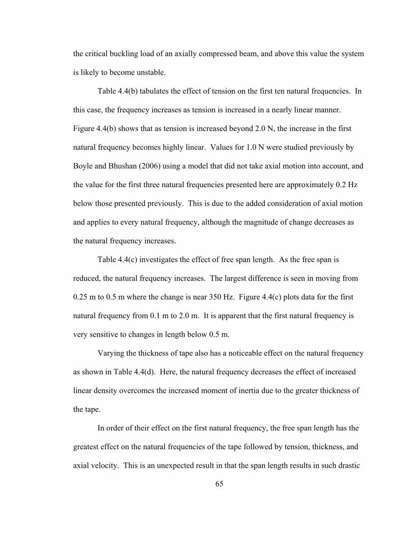
65
the critical buckling load of an axially compressed beam, and above this value the system
is likely to become unstable.
Table 4.4(b) tabulates the effect of tension on the first ten natural frequencies. In
this case, the frequency increases as tension is increased in a nearly linear manner.
Figure 4.4(b) shows that as tension is increased beyond 2.0 N, the increase in the first
natural frequency becomes highly linear. Values for 1.0 N were studied previously by
Boyle and Bhushan (2006) using a model that did not take axial motion into account, and
the value for the first three natural frequencies presented here are approximately 0.2 Hz
below those presented previously. This is due to the added consideration of axial motion
and applies to every natural frequency, although the magnitude of change decreases as
the natural frequency increases.
Table 4.4(c) investigates the effect of free span length. As the free span is
reduced, the natural frequency increases. The largest difference is seen in moving from
0.25 m to 0.5 m where the change is near 350 Hz. Figure 4.4(c) plots data for the first
natural frequency from 0.1 m to 2.0 m. It is apparent that the first natural frequency is
very sensitive to changes in length below 0.5 m.
Varying the thickness of tape also has a noticeable effect on the natural frequency
as shown in Table 4.4(d). Here, the natural frequency decreases the effect of increased
linear density overcomes the increased moment of inertia due to the greater thickness of
the tape.
In order of their effect on the first natural frequency, the free span length has the
greatest effect on the natural frequencies of the tape followed by tension, thickness, and
axial velocity. This is an unexpected result in that the span length results in such drastic
66
changes and high natural frequencies in the 0.25 m range corresponding to commercial
drives. Changes in tension are generally linear for any tension on the tape and are only
moderately sensitive to changes in magnitude. Tape thickness has a small effect on the
natural frequencies in the range of available tapes studied. The 14.4 µm tape is an
outdated tape thickness that was studied for comparison to historical data. Current
technology is the 9.0 µm tape, with 6.5 µm representing the next step in data storage tape
thickness. Due to the low axial velocities, relative to the critical speed, changes in the
natural frequencies are negligible. Although at higher velocities, this is not the case, and
even at these low velocities, the effect on the mode shapes can be seen.
4.5.1.2 Mode shapes
Coriolis acceleration of the system results in distortion of the mode shapes from
those for a stationary beam when axial velocity is considered. Figure 4.5 shows the first
four mode shapes for 0.5 m of 6.5 µm thick tape at 0.5 N of tension at 0 m/s, 8 m/s, and
20 m/s illustrating the effect of axial motion on the mode shapes. Each plot is composed
of the 0 m/s mode shape and the real and imaginary components of the mode shapes for 8
m/s and 20 m/s. As axial velocity is increased, the peak of the real component moves
slightly in the direction of motion, in this case to the right, and the imaginary component
shifts the same amount in the opposite direction. Since the final mode shape produced by
this analysis depends on the forcing function, it is necessary to present the real and
imaginary components separately for this general case. Also, as the velocity increases,
the magnitude of the real component of the mode shapes increases. In the second mode
and higher, the difference in magnitude becomes greater at each peak due to axial motion
67
Fig. 4.5 The first four mode shapes with varying axial velocities. Increasing axial
velocity results in real components of the mode shapes being shifted in the direction of
motion, to the right, and increases the amplitude of successive peaks. The opposite is
true for the imaginary components of the mode shapes in regards to both shifting and
amplitude in successive peaks.
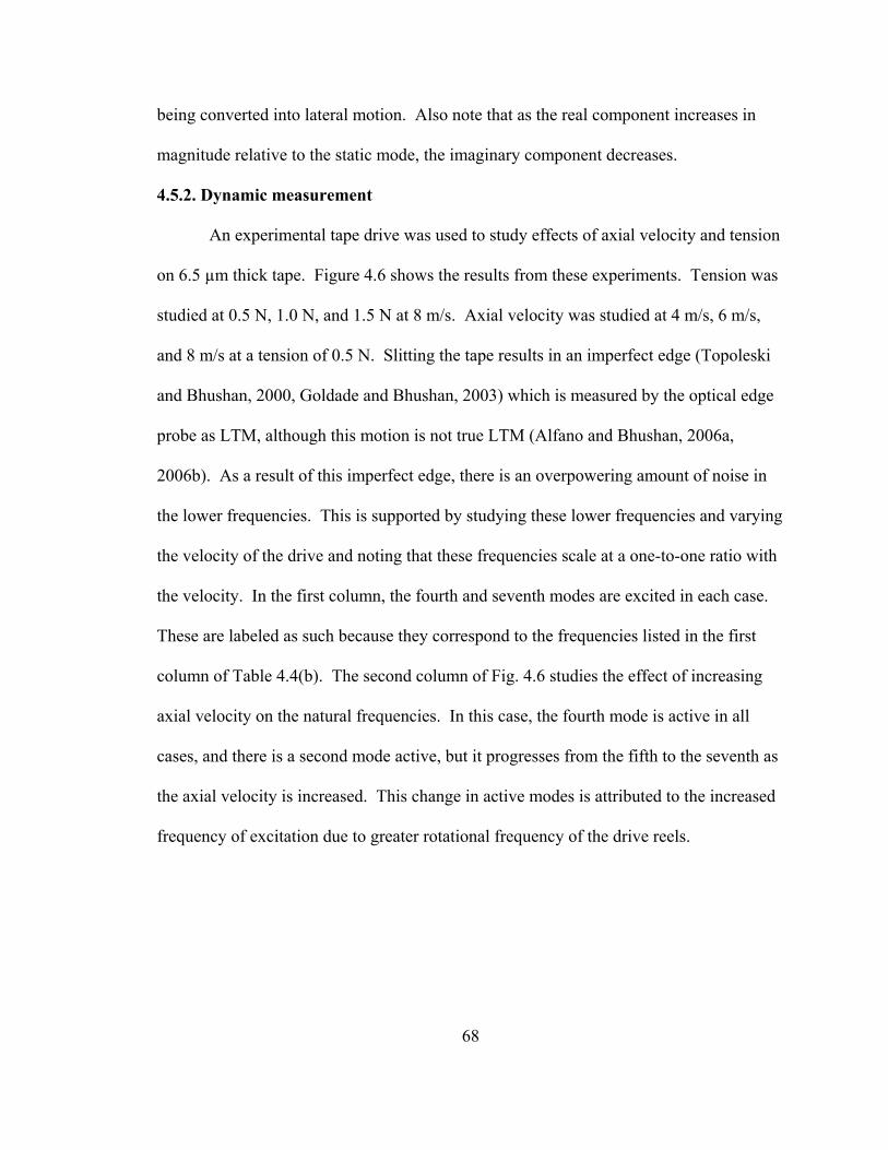
68
being converted into lateral motion. Also note that as the real component increases in
magnitude relative to the static mode, the imaginary component decreases.
4.5.2. Dynamic measurement
An experimental tape drive was used to study effects of axial velocity and tension
on 6.5 µm thick tape. Figure 4.6 shows the results from these experiments. Tension was
studied at 0.5 N, 1.0 N, and 1.5 N at 8 m/s. Axial velocity was studied at 4 m/s, 6 m/s,
and 8 m/s at a tension of 0.5 N. Slitting the tape results in an imperfect edge (Topoleski
and Bhushan, 2000, Goldade and Bhushan, 2003) which is measured by the optical edge
probe as LTM, although this motion is not true LTM (Alfano and Bhushan, 2006a,
2006b). As a result of this imperfect edge, there is an overpowering amount of noise in
the lower frequencies. This is supported by studying these lower frequencies and varying
the velocity of the drive and noting that these frequencies scale at a one-to-one ratio with
the velocity. In the first column, the fourth and seventh modes are excited in each case.
These are labeled as such because they correspond to the frequencies listed in the first
column of Table 4.4(b). The second column of Fig. 4.6 studies the effect of increasing
axial velocity on the natural frequencies. In this case, the fourth mode is active in all
cases, and there is a second mode active, but it progresses from the fifth to the seventh as
the axial velocity is increased. This change in active modes is attributed to the increased
frequency of excitation due to greater rotational frequency of the drive reels.
69
Fig. 4.6 Study of the effects of varying tension and velocity on the frequency components
of dynamic tape. Excited modes corresponding to the reel-to-reel free span length can be
seen in each plot.
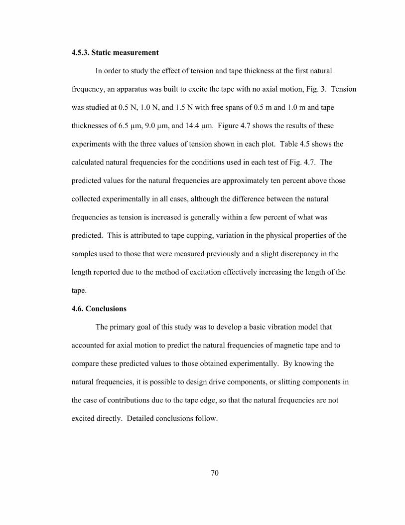
70
4.5.3. Static measurement
In order to study the effect of tension and tape thickness at the first natural
frequency, an apparatus was built to excite the tape with no axial motion, Fig. 3. Tension
was studied at 0.5 N, 1.0 N, and 1.5 N with free spans of 0.5 m and 1.0 m and tape
thicknesses of 6.5 µm, 9.0 µm, and 14.4 µm. Figure 4.7 shows the results of these
experiments with the three values of tension shown in each plot. Table 4.5 shows the
calculated natural frequencies for the conditions used in each test of Fig. 4.7. The
predicted values for the natural frequencies are approximately ten percent above those
collected experimentally in all cases, although the difference between the natural
frequencies as tension is increased is generally within a few percent of what was
predicted. This is attributed to tape cupping, variation in the physical properties of the
samples used to those that were measured previously and a slight discrepancy in the
length reported due to the method of excitation effectively increasing the length of the
tape.
4.6. Conclusions
The primary goal of this study was to develop a basic vibration model that
accounted for axial motion to predict the natural frequencies of magnetic tape and to
compare these predicted values to those obtained experimentally. By knowing the
natural frequencies, it is possible to design drive components, or slitting components in
the case of contributions due to the tape edge, so that the natural frequencies are not
excited directly. Detailed conclusions follow.
71
Fig. 4.7 Amplitude ratio versus frequency for the static test as tension, free span length,
and tape thickness are varied with three values of tension shown in each plot. The value
of the first natural frequency increases with increased tension and decreases with
increased free span length as predicted by the vibration model.
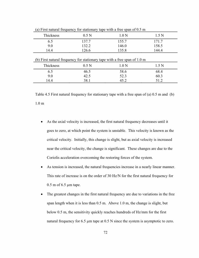
72
(a) First natural frequency for stationary tape with a free span of 0.5 m
Thickness 0.5 N 1.0 N 1.5 N 6.5 137.7 155.7 171.7 9.0 132.2 146.0 158.5 14.4 126.6 135.8 144.4 (b) First natural frequency for stationary tape with a free span of 1.0 m
Thickness 0.5 N 1.0 N 1.5 N 6.5 46.5 58.6 68.4 9.0 42.5 52.3 60.3 14.4 38.1 45.2 51.2 Table 4.5 First natural frequency for stationary tape with a free span of (a) 0.5 m and (b)
1.0 m
• As the axial velocity is increased, the first natural frequency decreases until it
goes to zero, at which point the system is unstable. This velocity is known as the
critical velocity. Initially, this change is slight, but as axial velocity is increased
near the critical velocity, the change is significant. These changes are due to the
Coriolis acceleration overcoming the restoring forces of the system.
• As tension is increased, the natural frequencies increase in a nearly linear manner.
This rate of increase is on the order of 30 Hz/N for the first natural frequency for
0.5 m of 6.5 µm tape.
• The greatest changes in the first natural frequency are due to variations in the free
span length when it is less than 0.5 m. Above 1.0 m, the change is slight, but
below 0.5 m, the sensitivity quickly reaches hundreds of Hz/mm for the first
natural frequency for 6.5 µm tape at 0.5 N since the system is asymptotic to zero.

73
• Increasing tape thickness results in a decrease of the natural frequencies since the
increased mass of the system reduces the natural frequencies to a greater degree
than the increased moment of inertia increases them.
• Simulation of the natural frequencies with the addition of axial motion resulted in
a negligible decrease as compared to those obtained using a stationary model.
This would suggest that as long as the axial velocity is below approximately ten
percent of the critical velocity, since the gyroscopic forces are still relatively
insignificant in this region, the difference between the two methods could be
insignificant depending on application.
• Axial motion results in a distortion of the mode shapes, causing a nonsymmetrical
profile with respect to the mid point of the tape. This is another effect of the
Coriolis acceleration where the axial motion of the tape resists the motion of
traveling lateral vibrations.
• There is a strong correlation between the predicted natural frequencies and those
measured experimentally in both the static and dynamic methods, implying that
the initial assumption that the tape path can be represented as a fixed-fixed beam
without any external forces is valid.

74
In order to improve and expand this model to better represent a real tape path,
damping from the tape, guides, and head should be considered in addition to the effect of
tape-to-guide impacts. The static vibration test could also prove to be useful in
examining mechanical properties of tape and any relationship to the degree of cupping to
the natural frequencies should be investigated.
75
CHAPTER 5
SUMMARY
In order to successfully increase the storage capacity of magnetic tape, the
substrate and layers must be made thinner and the number of data tracks must be
increased while the width and spacing between the tracks must be decreased. As the
tracks become narrower and closer together, lateral tape motion (LTM) becomes a
significant obstacle. In order to minimize LTM, the sources and mechanics need to be
understood. As part of understanding, the ability to accurately measure the true LTM is
necessary to gain insight to the motion of the tape as the head experiences it.
In studying the effects of tape thickness on tribological and magnetic durability
and LTM, several findings were made. First, tapes with thinner substrates are more
prone to produce debris due to increased stresses caused by edge impacts and compliance
resulting in cracking of the coatings. LTM for the thinner tape was less than that for the
thicker tape, and this is attributed to the increased friction of the thinner tape due to
smoother coatings and increased compliance. Magnetically, there was no significant
difference attributable to the substrate.
To measure the true LTM, a method of monitoring a simulated magnetic signal
with a video camera was developed. This method proved to be successful in rejecting
edge defect contributions as well as repeatable tape motion while making measurements
on the order of 1 µm. The primary limitation of the method used was the sampling rate

76
of the equipment, which ideally would be thousands of frames per second in order to
measure high frequency LTM.
Understanding of the mechanics of a magnetic tape with axial motion was
improved by implementing a vibration model to predict the natural frequencies and mode
shapes of various operating conditions. The results of the vibration model were
confirmed with experimental results of both dynamic and static experiments. Gyroscopic
forces due to axial motion result in lower natural frequencies for increased motion than
those for a static beam and a distortion of the mode shapes.

77
APPENDIX A
DROUPOUT COUNTER CODE
This QuickBASIC 4.5 program initializes, starts, and retrieves data from the
dropout counter. The retrieved data is then stored to the specified file.
QUICKBASIC CODE
DECLARE SUB WriteDrop (pass%) ' This file includes all function DECLARAtion supported by the DAQ driver. ' $INCLUDE: 'Q4IFACE.BI' '***************************************************************************** DECLARE SUB BootSeq () DECLARE SUB BuildTestParams () DECLARE SUB ContTest (time) DECLARE SUB DComms (d$) DECLARE SUB ShowData () TYPE DepthParm START AS SINGLE stp AS SINGLE BurWid AS SINGLE BurRate AS SINGLE END TYPE '----------------------------------------------------------------------------- DIM SHARED DoDepth(4) AS DepthParm, DOWidth(5), docount(20), BurstCount(4) COMMON SHARED DorCmd$, DorResp$, TestParams$, CountTime, DorStat, in$ COMMON SHARED /File/ fault COMMON SHARED /Dorad/ DownLoad$, DropParam$, burstlkout$ COMMON SHARED /Dorad/ TestSet$, testtime$, time COMMON SHARED /STATUS/ DorStatCode
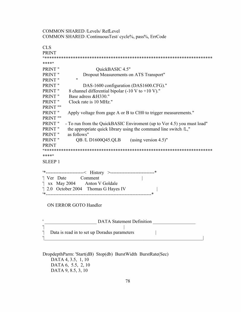
78
COMMON SHARED /Levels/ RefLevel COMMON SHARED /ContinuousTest/ cycle%, pass%, ErrCode CLS PRINT "***************************************************************************" PRINT " QuickBASIC 4.5" PRINT " Dropout Measurements on ATS Transport" PRINT " " PRINT " DAS-1600 configuration (DAS1600.CFG)." PRINT " 8 channel differential bipolar (-10 V to +10 V)." PRINT " Base adress &H330." PRINT " Clock rate is 10 MHz." PRINT "" PRINT " Apply voltage from gage A or B to CH0 to trigger measurements." PRINT "" PRINT " - To run from the QuickBASIC Enviroment (up to Ver 4.5) you must load" PRINT " the appropriate quick library using the command line switch /L," PRINT " as follows" PRINT " QB /L D1600Q45.QLB (using version 4.5)" PRINT "***************************************************************************" SLEEP 1 '*------------------------< History >----------------------------* '| Ver Date Comment | '| xx May 2004 Anton V Goldale '| 2.0 October 2004 Thomas G Hayes IV | '*-------------------------------------------------------------------* ON ERROR GOTO Handler ' ______________________ DATA Statement Definition __________________ '| | '| Data is read in to set up Doradus parameters | '|___________________________________________________________________| DropdepthParm: 'Start(dB) Stop(db) BurstWidth BurstRate(Sec) DATA 4, 3.5, 1, 10 DATA 6, 5.5, 2, 10 DATA 9, 8.5, 3, 10

79
DATA 12, 11.5, 4, 10 DropwidthParm: 'MicroSeconds DATA 0.5 DATA 1 DATA 5 DATA 10 DATA 25 '----------------------------- End Data ------------------------------- WaitTime% = 1 'Time to wait before sending next command to the tester CountTime = 10 'Duration of the COUNT step in seconds 'ON ERROR GOTO Handler ON KEY(31) GOSUB HotKey DorCmd$ = "" CALL BuildTestParams CALL BootSeq CALL ContTest(time) 1 END Handler: fault = ERR SELECT CASE ERR CASE 58: Error$ = "Duplicate file. " ' CALL message(Error$ + "Select another filename. ") fault = 0 RESUME NEXT CASE 200: LOCATE 21, 11: COLOR 4, 0 PRINT "Test Interrupt Initiated. Please standby...!" RESUME NEXT fault = 0 CASE ELSE: RESUME NEXT END SELECT HotKey: ' CALL Doradus("Abort", "", 1) CLOSE #100 GOTO 1 RETURN '=============================< End Main > ==================================
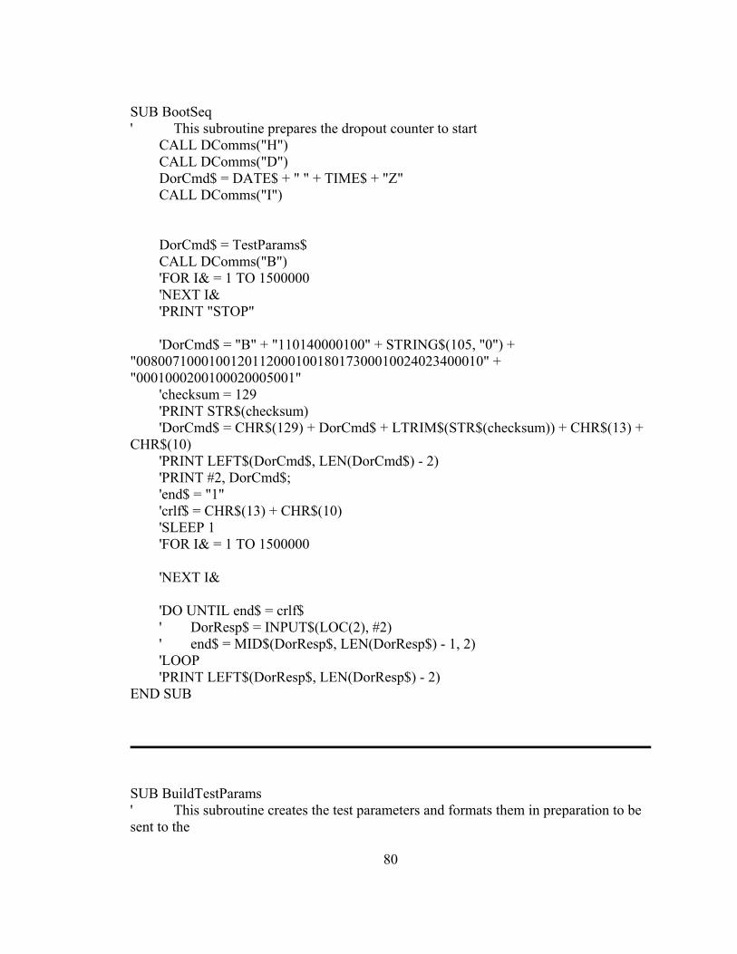
80
SUB BootSeq ' This subroutine prepares the dropout counter to start CALL DComms("H") CALL DComms("D") DorCmd$ = DATE$ + " " + TIME$ + "Z" CALL DComms("I") DorCmd$ = TestParams$ CALL DComms("B") 'FOR I& = 1 TO 1500000 'NEXT I& 'PRINT "STOP" 'DorCmd$ = "B" + "110140000100" + STRING$(105, "0") + "008007100010012011200010018017300010024023400010" + "0001000200100020005001" 'checksum = 129 'PRINT STR$(checksum) 'DorCmd$ = CHR$(129) + DorCmd$ + LTRIM$(STR$(checksum)) + CHR$(13) + CHR$(10) 'PRINT LEFT$(DorCmd$, LEN(DorCmd$) - 2) 'PRINT #2, DorCmd$; 'end$ = "1" 'crlf$ = CHR$(13) + CHR$(10) 'SLEEP 1 'FOR I& = 1 TO 1500000 'NEXT I& 'DO UNTIL end$ = crlf$ ' DorResp$ = INPUT$(LOC(2), #2) ' end$ = MID$(DorResp$, LEN(DorResp$) - 1, 2) 'LOOP 'PRINT LEFT$(DorResp$, LEN(DorResp$) - 2) END SUB
SUB BuildTestParams ' This subroutine creates the test parameters and formats them in preparation to be sent to the
81
' Dropout counter testnum$ = "1" pulseflag$ = "1" sampleperiod$ = "010" minutes$ = "000" seconds$ = "01" outpattern$ = "00" testset2$ = "04" + STRING$(98, "0") burstlkout$ = "01" testtime$ = RIGHT$("00000" + LTRIM$(STR$(CountTime)), 5) TestParams$ = testnum$ + pulseflag$ + sampleperiod$ + minutes$ + seconds$ + outpattern$ + testtime$ + testset2$ RESTORE DropdepthParm FOR I = 1 TO 4 READ DoDepth(I).START, DoDepth(I).stp, DoDepth(I).BurWid, DoDepth(I).BurRate NEXT I RESTORE DropwidthParm FOR I = 1 TO 5 READ DOWidth(I) NEXT I DropParam$ = "" FOR I = 1 TO 4 strt$ = RIGHT$("000" + LTRIM$(STR$(DoDepth(I).START * 2)), 3) stop$ = RIGHT$("000" + LTRIM$(STR$(DoDepth(I).stp * 2)), 3) burstwid$ = LTRIM$(STR$(DoDepth(I).BurWid)) burstrate$ = RIGHT$("00000" + LTRIM$(STR$(DoDepth(I).BurRate)), 5) DropParam$ = DropParam$ + strt$ + stop$ + burstwid$ + burstrate$ NEXT I FOR I = 1 TO 5 DOWidth$ = RIGHT$("0000" + LTRIM$(STR$(DOWidth(I) * 2)), 4) DropParam$ = DropParam$ + DOWidth$ NEXT I TestParams$ = TestParams$ + DropParam$ + burstlkout$ PRINT TestParams$ END SUB

82
SUB ContTest (time) ' This is the main loop of the program where the trigger input is monitored ' and the dropout counter is instructed to begin monitoring the signal. After ' the spcified time is up the data is read from the dropout counter and stored ' then the droupout counter is cleared and initialized in preparation for the ' next pass DIM BUFFA(1000) AS INTEGER DIM NumOfBoards AS INTEGER DIM DERR AS INTEGER DIM DEVHANDLE AS LONG DIM ADHANDLE AS LONG DIM STATUS AS INTEGER DIM count AS LONG PRINT "Input name of file:": INPUT in$ KEY(31) ON cycle% = 1 pass% = 1 DO 'STEP 1: A$ = "DAS1600.CFG" + CHR$(0) DERR = DAS1600DEVOPEN%(SSEGADD(A$), NumOfBoards) IF DERR <> 0 THEN BEEP: PRINT "ERROR "; HEX$(DERR); " OCCURRED DURING 'DEVOPEN'" 'STEP 2: DERR = DAS1600GETDEVHANDLE%(0, DEVHANDLE) IF DERR <> 0 THEN BEEP: PRINT "ERROR "; HEX$(DERR); "OCCURRED DURING 'GET DEVHANDLE'": STOP 'STEP 3: DERR = KGetADFrame%(DEVHANDLE, ADHANDLE) IF DERR <> 0 THEN BEEP: PRINT "ERROR "; HEX$(DERR); "OCCURRED DURING 'KGetADFrame'": STOP 'STEP 4: DAS1600ERR = KSetBufI%(ADHANDLE, BUFFA(0), 1000) IF DAS1600ERR <> 0 THEN BEEP: PRINT "ERROR "; HEX$(DAS1600ERR); "OCCURRED DURING 'KSetBufI'": STOP 'STEP 5: DERR = KSetClkRate%(ADHANDLE, 1000)

83
IF DERR <> 0 THEN BEEP: PRINT "ERROR "; HEX$(DERR); " OCCURRED DURING 'KSetClkRate'": STOP 'STEP 6: DERR = KSetTrig%(ADHANDLE, 1) IF DERR <> 0 THEN BEEP: PRINT "ERROR "; HEX$(DERR); " OCCURRED DURING 'KSetTrig'": STOP 'STEP 7: LEVEL = 2260: OPT = 0: CHAN = 0 DERR = KSetADTrig%(ADHANDLE, OPT, CHAN, LEVEL) IF DERR <> 0 THEN BEEP: PRINT "ERROR "; HEX$(DERR); " OCCURRED DURING 'KSetADTrig'": STOP 'STEP 8: DERR = KSetTrigHyst%(ADHANDLE, &H10) IF DERR <> 0 THEN BEEP: PRINT "ERROR "; HEX$(DERR); " OCCURRED DURING 'KSetTrigHyst'": STOP IF pass% = 1 THEN PRINT "Waiting for the beginning of cycle..." END IF 'STEP 9: DERR = KINTStart%(ADHANDLE) IF DERR <> 0 THEN BEEP: PRINT "ERROR "; HEX$(DERR); " OCCURRED DURING 'KINT'": STOP SELECT CASE pass% CASE 1 ' PRINT "CYCLE "; cycle%; ". Forward pass started." CASE 2 ' PRINT "CYCLE "; cycle%; ". Reverse pass started." END SELECT 'STEP 10: DERR = KINTStatus%(ADHANDLE, STATUS, count) IF DERR <> 0 THEN BEEP: PRINT "ERROR "; HEX$(DERR); " OCCURRED DURING 'KINTStatus'" 'STEP 11: DERR = KFreeFrame%(ADHANDLE)

84
IF DERR <> 0 THEN BEEP: PRINT "ERROR "; HEX$(DERR); " OCCURRED DURING 'KFreeFrame'": STOP CALL DComms("H") CALL DComms("D") DorCmd$ = DATE$ + " " + TIME$ + "Z" CALL DComms("I") CALL DComms("E") SleepTime = CountTime + 1 SLEEP SleepTime CALL DComms("A") IF (DorStat AND 4) = 0 THEN CALL WriteDrop(pass%) ELSE CALL DComms("H") CALL WriteDrop(pass%) END IF SELECT CASE pass% CASE 1 PRINT "Cycle "; cycle%; ". Forward pass done." pass% = 2 CASE 2 PRINT "Cycle "; cycle%; ". Reverse pass done." pass% = 1 cycle% = cycle% + 1 END SELECT CALL ShowData LOOP KEY(31) OFF END SUB
SUB DComms (d$) ' This subroutine handles the communication with the dropout counter through ' the serial port COM2 DorResp$ = "" end$ = "1" crlf$ = CHR$(13) + CHR$(10)
85
OPEN "COM2:9600,N,8,1" FOR RANDOM AS #2 checksum = 129 XOR ASC(d$) IF DorCmd$ <> "" THEN FOR J% = 1 TO LEN(DorCmd$) checksum = checksum XOR ASC(MID$(DorCmd$, J%, 1)) NEXT J% PRINT "checksum done" DorCmd$ = CHR$(129) + d$ + DorCmd$ + LTRIM$(STR$(checksum)) + CHR$(13) + CHR$(10) ELSE DorCmd$ = CHR$(129) + d$ + LTRIM$(STR$(checksum)) + CHR$(13) + CHR$(10) END IF PRINT LEFT$(DorCmd$, LEN(DorCmd$) - 2) PRINT #2, DorCmd$; FOR I& = 1 TO 1600000 NEXT I& DorResp$ = INPUT$(LOC(2), #2) end$ = MID$(DorResp$, LEN(DorResp$) - 1, 2) IF end$ <> crlf$ THEN PRINT "Communications Error" END IF PRINT LEFT$(DorResp$, LEN(DorResp$) - 2) DorStat = VAL(MID$(DorResp$, 3, 3)) PRINT "DorStat:"; DorStat DorCmd$ = "" FOR I& = 1 TO 1600000 NEXT I& END SUB
SUB ShowData ' This subroutine displays a table of the dropout data after each pass as was ' reported by the dropout counter PRINT "Test #: "; MID$(DorResp$, 12, 20) J = 1 FOR I = 32 TO 127 STEP 5 PRINT MID$(DorResp$, I, 5) + " "; IF J = 5 THEN PRINT ""

86
J = 0 END IF J = J + 1 NEXT I 'FOR I = 131 TO 137 STEP 2 ' Drop$ = Drop$ + MID$(DorResp$, I, 2) + ", " 'NEXT I 'Drop$ = Drop$ + MID$(DorResp$, 139, 4) + ", " + MID$(DorResp$, 143, 3) END SUB
SUB WriteDrop (pass%) ' This subroutine writes the data from the dropout counter to the spcified file CALL DComms("F") Drop$ = "" Drop$ = MID$(DorResp$, 12, 20) + ", " FOR I = 32 TO 127 STEP 5 Drop$ = Drop$ + MID$(DorResp$, I, 5) + ", " NEXT I FOR I = 133 TO 138 STEP 2 Drop$ = Drop$ + MID$(DorResp$, I, 2) + ", " NEXT I Drop$ = Drop$ + MID$(DorResp$, 140, 4) + ", " + MID$(DorResp$, 144, 3) OPEN in$ FOR APPEND AS #100 PRINT #100, LTRIM$(STR$(cycle%)); ","; STR$(pass%); ", "; Drop$ CLOSE #100 END SUB
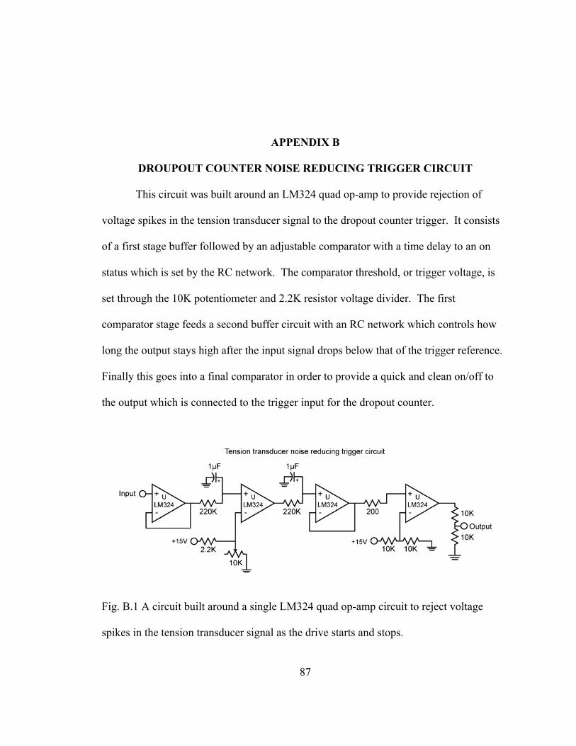
87
APPENDIX B
DROUPOUT COUNTER NOISE REDUCING TRIGGER CIRCUIT
This circuit was built around an LM324 quad op-amp to provide rejection of
voltage spikes in the tension transducer signal to the dropout counter trigger. It consists
of a first stage buffer followed by an adjustable comparator with a time delay to an on
status which is set by the RC network. The comparator threshold, or trigger voltage, is
set through the 10K potentiometer and 2.2K resistor voltage divider. The first
comparator stage feeds a second buffer circuit with an RC network which controls how
long the output stays high after the input signal drops below that of the trigger reference.
Finally this goes into a final comparator in order to provide a quick and clean on/off to
the output which is connected to the trigger input for the dropout counter.
Fig. B.1 A circuit built around a single LM324 quad op-amp circuit to reject voltage
spikes in the tension transducer signal as the drive starts and stops.

88
APPENDIX C
PSD SPECTRUM MATLAB CODE
This code is used to create power spectrum density plots (PSD) and frequency
spectrum plots from an ascii plotter file (.plt) without headers and normally just one or
two columns although more can be accommodated.
MATLAB CODE
% 12/9/04 Commented out multiplication factor for column 2 % 08/14/06 Added a user interface to open files rather than typing the path % and file name into the matlab command window clear; clc; [file_name, pathname] = uigetfile('*.plt', 'Pick a 4 m/s plt file'); if isequal(file_name,0) disp('User selected Cancel') else disp(['User selected', fullfile(pathname, file_name)]) end z=load(fullfile(pathname, file_name)); %samp_rate=input('Input sampling rate, in Hz: '); % fprintf('How many lines per second for waterfall plot generation? \n'); % fprintf('(Note: 1 line per second gives 1 Hz frequency resolution. Increasing \n'); % fprintf('lines per second decreases frequency resolution by same factor) \n'); % res=input(''); % Since the sample rate and desired resolution is usually constant for a % set of files it's usually easier to just define it rather than type it in % each time samp_rate=7544; res=1;

89
%% These are start and end times of fwd. and rev. pass for use in average %% power spectrum calculation. t1 = start of fwd, t2 = end of fwd, t3 = %% start of rev, t4 = end of rev. Note: these "times" really refer to %% columns of z_parsed (and Pyy): column 1 is 0-1 sec, col 2 is 1-2 sec, etc. So to %% start analysis at 1 sec, t1 must = 2. t1=3; t2=23; t3=29; t4=49; % Nyquist frequency always equals 1/2 sampling rate nyquist=samp_rate/2; N_z=length(z); % If file contains multiple columns, break it into multiple column vectors size_z=size(z); Nc_z=size_z(2); clear size_z; z1=z(:,1); if Nc_z > 1 z2=z(:,2); if Nc_z > 2 z3=z(:,3); if Nc_z > 3 z4=z(:,4); if Nc_z > 4 z5=z(:,5); end end end end clear z; %%%%%%%%%%%%%%%%%%%%%%%%%%%%%%%%%%%%%%%%%%% % This program can perform spectrum analysis on any signal. I assume one % or more columns contain LTM data. Below, multiply column(s) by the edge probe's % calibration factor(s) (micron/volt) z1=z1.*17.853; % z2=z2.*14.853;

90
%%%%%%%%%%%%%%%%%%%%%%%%%%%%%%%%%%%%%%%%%%%%%%%%%%%%%%%%%%%%%%%%%%%%%%%%% % Normalize tension transducer data (rescale one transducer signal to match % the scale of the other). In this case, columns 1 and 2 are the tension % signals and column 2 is scaled to match column 1 % z1_avg = mean(z1); % z2_avg = mean(z2); % z1 = (z1./z1_avg).*z2_avg; % clear z1_avg z2_avg; %%%%%%%%%%%%%%%%%%%%%%%%%%%%%%%%%%%%%%%%%%%%%%%%%%%%%%%%%%%%%%%%%%%%%%%%%% %%%%%%%%%%%%%%%%%%%% % Column 1 %%%%%%%%%%%%%%%%%%%% % Notes: % 1) The frequency values computed by the fft function correspond to % frequencies separated by 1/NT Hertz, where N = the number of points and % T= the sampling period (= 1/samp_rate), in sec. % 2) Since the discreet Fourier transform is a periodic function, the % values above the Nyquist frequency do not represent new information, so % only the first half of the fft output is kept. % Break file into columns of length samp_rate/res % Create corresponding time and frequency matrices z1_parsed(:,1)=z1(1:samp_rate/res); freq(:,1)=(0:res:nyquist)'; time(1:0.5*samp_rate/res+1,1)=1/res; i=1; while (i+1)*samp_rate/res < N_z z1_parsed(:,i+1)=z1(i*samp_rate/res+1:(i+1)*samp_rate/res); freq(:,i+1)= (0:res:nyquist)'; time(1:0.5*samp_rate/res+1,i+1)=(i+1)/res; i=i+1; end % Separate forward and reverse passes z1_parsed_fwd=z1_parsed(:,t1:t2); z1_parsed_rev=z1_parsed(:,t3:t4); % Create forward and reverse pass vectors for coherence calculation
91
z1_fwd=z1(samp_rate*t1:samp_rate*t2); z1_rev=z1(samp_rate*t3:samp_rate*t4); % Perform fft y1_fwd=fft(z1_parsed_fwd); y1_rev=fft(z1_parsed_rev); % Delete second half of freq. domain values (redundant part) N_y1_fwd=length(y1_fwd); y1_fwd=y1_fwd(1:N_y1_fwd/2+1,:); N_y1_rev=length(y1_rev); y1_rev=y1_rev(1:N_y1_rev/2+1,:); % Take magnitude of the fft and scale by length of input y1_fwd=abs(y1_fwd); y1_fwd=y1_fwd/length(z1_parsed_fwd); y1_rev=abs(y1_rev); y1_rev=y1_rev/length(z1_parsed_rev); % Compute power spectrum Pyy1_fwd=y1_fwd.^2; Pyy1_rev=y1_rev.^2; % Multiply values (except DC and nyquist components) by 2 because % we threw out half of values Pyy1_fwd(2:(length(Pyy1_fwd)-1),:)=Pyy1_fwd(2:(length(Pyy1_fwd)-1),:).*2; Pyy1_fwd(2:(length(Pyy1_fwd)-1),:)=Pyy1_fwd(2:(length(Pyy1_fwd)-1),:).*2; % Throw out DC component Pyy1_fwd(1,:)=[]; Pyy1_rev(1,:)=[]; freq(1,:)=[]; time(1,:)=[]; % Compute average power spectrum for each frequency over range of % times specified. i=1; while i <= (samp_rate/res)/2 Pyy1avgfwd(i) = mean(Pyy1_fwd(i,:)); Pyy1avgrev(i) = mean(Pyy1_rev(i,:)); i=i+1; end % Combine forward and reverse pass spectrums into one variable for

92
% waterfall plotting. Add columns of zeros for times when power spectrum % was not computed (i.e. at start/stop) i=0; while t1+i<=t2 Pyy1_comb(:,t1+i)=Pyy1_fwd(:,i+1); i=i+1; end temp=t1-1; while temp>0 Pyy1_comb(:,temp)=0; temp=temp-1; end temp=t3-t2-1; while t2+temp>t2 Pyy1_comb(:,t2+temp)=0; temp=temp-1; end i=0; while t3+i<=t4 Pyy1_comb(:,t3+i)=Pyy1_rev(:,i+1); i=i+1; end dummy=size(time); Nc_time=dummy(2); temp=t4+1; while temp<=Nc_time Pyy1_comb(:,temp)=0; temp=temp+1; end clear temp dummy; % Transpose matrices and create waterfall plot of data Pyy1_comb=Pyy1_comb'; time=time'; freq=freq'; figure(1); %waterfall(freq,time,Pyy1_comb); hhh = meshz(freq,time,Pyy1_comb); axis([0 200 0 Nc_time 0 40]); set(hhh,'MeshStyle','row'); grid off;
93
xlabel('Frequency (Hz)'); ylabel('time (sec)'); zlabel('Power'); title(file_name); % map defines the colors used. [0 0 0;0 0 0] is all black map = [0 0 0;0 0 0]; colormap(map); z_max1 = max(Pyy1_comb); z_max = [0 max(z_max1)]; clear z_max1; % set the X,Y,Z axis range %set(gca,'XLim',[0 200],'YLim',[0 Nc_time],'ZLim',[0 40]); % set the view point [azimuth elevation] view([-5 30]); set(gcf,'name','column 1 data','NumberTitle','off') figure(2); plot(freq(1,:),log(Pyy1avgfwd),'k'); xlabel('Frequency (Hz)'); ylabel('Average Power'); title(file_name); set(gca,'XLim',[0 3500]); text_x_loc= 250; text_y_loc=max(Pyy1avgfwd); text(text_x_loc,text_y_loc,['fwd pass'],'BackgroundColor',[1 1 1],'HorizontalAlignment','center'); set(gcf,'name','column 1 data','NumberTitle','off') % % figure; % plot(freq(1,:),Pyy1avgrev,'k'); % xlabel('Frequency (Hz)'); % ylabel('Average Power'); % title(file_name); % set(gca,'XLim',[0 800]); % text_x_loc= 250; % text_y_loc=max(Pyy1avgrev); % text(text_x_loc,text_y_loc,['rev pass'],'BackgroundColor',[1 1 1],'HorizontalAlignment','center'); % set(gcf,'name','column 1 data','NumberTitle','off') % % % Delete extra variables
94
% clear z1 y1_fwd y2_rev z1_parsed z1_parsed_fwd z1_parsed_rev N_y1_fwd N_y1_rev; % % %%%%%%%%%%%%%%%%%%%%%%%%%%%%%%%%% % % Column 2 % %%%%%%%%%%%%%%%%%%%%%%%%%%%%%%%%% % % if Nc_z > 1 % % z2_parsed(:,1)=z2(1:samp_rate/res); % i=1; % while (i+1)*samp_rate/res < N_z % z2_parsed(:,i+1)=z2(i*samp_rate/res+1:(i+1)*samp_rate/res); % i=i+1; % end % % % % Separate forward and reverse passes % z2_parsed_fwd=z2_parsed(:,t1:t2); % z2_parsed_rev=z2_parsed(:,t3:t4); % % % Create forward and reverse pass vectors for coherence calculation % z2_fwd=z2(samp_rate*t1:samp_rate*t2); % z2_rev=z2(samp_rate*t3:samp_rate*t4); % % % Subtract out average tape position for fwd and rev passes % z2_parsed_fwd=z2_parsed_fwd-mean(z2_parsed_fwd(:)); % z2_parsed_rev=z2_parsed_rev-mean(z2_parsed_rev(:)); % % % Perform fft % y2_fwd=fft(z2_parsed_fwd); % y2_rev=fft(z2_parsed_rev); % % % Delete second half of freq. domain values (redundant part) % N_y2_fwd=length(y2_fwd); % y2_fwd=y2_fwd(1:N_y2_fwd/2+1,:); % N_y2_rev=length(y2_rev); % y2_rev=y2_rev(1:N_y2_rev/2+1,:); % % % Take magnitude of the fft and scale by length of input % y2_fwd=abs(y2_fwd); % y2_fwd=y2_fwd/length(z2_parsed_fwd); % y2_rev=abs(y2_rev); % y2_rev=y2_rev/length(z2_parsed_rev); %

95
% % Compute power spectrum % Pyy2_fwd=y2_fwd.^2; % Pyy2_rev=y2_rev.^2; % % % Multiply values (except DC and nyquist components) by 2 because % % we threw out half of values % Pyy2_fwd(2:(length(Pyy2_fwd)-1),:)=Pyy2_fwd(2:(length(Pyy2_fwd)-1),:).*2; % Pyy2_fwd(2:(length(Pyy2_fwd)-1),:)=Pyy2_fwd(2:(length(Pyy2_fwd)-1),:).*2; % % % Throw out DC component % Pyy2_fwd(1,:)=[]; % Pyy2_rev(1,:)=[]; % % % % Compute average power spectrum for each frequency over range of % % times specified. % i=1; % while i <= (samp_rate/res)/2 % Pyy2avgfwd(i) = mean(Pyy2_fwd(i,:)); % Pyy2avgrev(i) = mean(Pyy2_rev(i,:)); % i=i+1; % end % % % Combine forward and reverse pass spectrums into one variable for % % waterfall plotting. Add columns of zeros for times when power spectrum % % was not computed (i.e. at start/stop) % % i=0; % while t1+i<=t2 % Pyy2_comb(:,t1+i)=Pyy2_fwd(:,i+1); % i=i+1; % end % temp=t1-1; % while temp>0 % Pyy2_comb(:,temp)=0; % temp=temp-1; % end % temp=t3-t2-1; % while t2+temp>t2 % Pyy2_comb(:,t2+temp)=0; % temp=temp-1; % end % i=0; % while t3+i<=t4 % Pyy2_comb(:,t3+i)=Pyy2_rev(:,i+1);
96
% i=i+1; % end % temp=t4+1; % while temp<=Nc_time % Pyy2_comb(:,temp)=0; % temp=temp+1; % end % clear temp dummy; % % % %%%%%%%%%%%%%%%%%%%%%%%%%%%%%%%%%%%%%%%%%%%%%%%%%%%%%%%%%%%%%%%%%%%%%%%%%%% % % Compute peak-peak LTM for each column of z_parsed (corresponding to time % % span of 1/res seconds) and report the max and mean values. Move and modify this % % section according to which column is LTM data. % % PPLTM_fwd=max(z2_parsed_fwd)-min(z2_parsed_fwd); % PPLTM_rev=max(z2_parsed_rev)-min(z2_parsed_rev); % max_LTM_fwd=max(PPLTM_fwd) % max_LTM_rev=max(PPLTM_rev) % mean_LTM_fwd=mean(PPLTM_fwd) % mean_LTM_rev=mean(PPLTM_rev) % clear dummy Nc_z2_parsed; % %%%%%%%%%%%%%%%%%%%%%%%%%%%%%%%%%%%%%%%%%%%%%%%%%%%%%%%%%%%%%%%%%%%%%%%%%%%% % % % Transpose matrices and create waterfall plot of data % Pyy2_comb=Pyy2_comb'; % % % figure; % waterfall(freq,time,Pyy2_comb); % xlabel('Frequency (Hz)'); % ylabel('time (sec)'); % zlabel('Power'); % title(file_name); % % map defines the colors used. [0 0 0;0 0 0] is all black % map = [0 0 0;0 0 0]; % colormap(map); % z_max1 = max(Pyy2_comb); % z_max = [0 max(z_max1)]; % clear z_max1;
97
% % set the X,Y,Z axis range % set(gca,'XLim',[0 200],'YLim',[0 Nc_time],'ZLim',z_max); % % set the view point [azimuth elevation] % view([-5 30]); % set(gcf,'name','column 2 data','NumberTitle','off') % % % figure; % plot(freq(1,:),Pyy2avgfwd,'k'); % xlabel('Frequency (Hz)'); % ylabel('Average Power'); % title(file_name); % set(gca,'XLim',[0 800]); % text_x_loc= 250; % text_y_loc=max(Pyy2avgfwd); % text(text_x_loc,text_y_loc,['fwd pass'],'BackgroundColor',[1 1 1],'HorizontalAlignment','center'); % set(gcf,'name','column 2 data','NumberTitle','off') % % figure; % plot(freq(1,:),Pyy2avgrev,'k'); % xlabel('Frequency (Hz)'); % ylabel('Average Power'); % title(file_name); % set(gca,'XLim',[0 800]); % text_x_loc= 250; % text_y_loc=max(Pyy2avgrev); % text(text_x_loc,text_y_loc,['rev pass'],'BackgroundColor',[1 1 1],'HorizontalAlignment','center'); % set(gcf,'name','column 2 data','NumberTitle','off') % % % Delete extra variables % clear z2 y2_fwd y2_rev z2_parsed z2_parsed_fwd z2_parsed_rev N_y2_fwd N_y2_rev; % % figure; % cohere(z1_fwd,z2_fwd,1024,samp_rate,'mean'); % title('Fwd pass coherence'); % % figure; % cohere(z1_rev,z2_rev,1024,samp_rate,'mean'); % title('Rev pass coherence'); % % % %%%%%%%%%%%%%%%%%%%%%%%%%%%%%%%%%
98
% % Column 3 % %%%%%%%%%%%%%%%%%%%%%%%%%%%%%%%%% % if Nc_z > 2 % z3_parsed(:,1)=z3(1:samp_rate/res); % % i=1; % while (i+1)*samp_rate/res < N_z % z3_parsed(:,i+1)=z3(i*samp_rate/res+1:(i+1)*samp_rate/res); % i=i+1; % end % % % Separate forward and reverse passes % z3_parsed_fwd=z3_parsed(:,t1:t2); % z3_parsed_rev=z3_parsed(:,t3:t4); % % % Subtract out average tape position for fwd and rev passes % z3_parsed_fwd=z3_parsed_fwd-mean(z3_parsed_fwd(:)); % z3_parsed_rev=z3_parsed_rev-mean(z3_parsed_rev(:)); % % % Perform fft % y3_fwd=fft(z3_parsed_fwd); % y3_rev=fft(z3_parsed_rev); % % % Delete second half of freq. domain values (redundant part) % N_y3_fwd=length(y3_fwd); % y3_fwd=y3_fwd(1:N_y3_fwd/2+1,:); % N_y3_rev=length(y3_rev); % y3_rev=y3_rev(1:N_y3_rev/2+1,:); % % % Take magnitude of the fft and scale by length of input % y3_fwd=abs(y3_fwd); % y3_fwd=y3_fwd/length(z3_parsed_fwd); % y3_rev=abs(y3_rev); % y3_rev=y3_rev/length(z3_parsed_rev); % % % Compute power spectrum % Pyy3_fwd=y3_fwd.^2; % Pyy3_rev=y3_rev.^2; % % % Multiply values (except DC and nyquist components) by 2 because % % we threw out half of values % Pyy3_fwd(2:(length(Pyy3_fwd)-1),:)=Pyy3_fwd(2:(length(Pyy3_fwd)-1),:).*2; % Pyy3_fwd(2:(length(Pyy3_fwd)-1),:)=Pyy3_fwd(2:(length(Pyy3_fwd)-1),:).*2; % % % Throw out DC component

99
% Pyy3_fwd(1,:)=[]; % Pyy3_rev(1,:)=[]; % % % % Compute average power spectrum for each frequency over range of % % times specified. % i=1; % while i <= (samp_rate/res)/2 % Pyy3avgfwd(i) = mean(Pyy3_fwd(i,:)); % Pyy3avgrev(i) = mean(Pyy3_rev(i,:)); % i=i+1; % end % % % Combine forward and reverse pass spectrums into one variable for % % waterfall plotting. Add columns of zeros for times when power spectrum % % was not computed (i.e. at start/stop) % % i=0; % while t1+i<=t2 % Pyy3_comb(:,t1+i)=Pyy3_fwd(:,i+1); % i=i+1; % end % temp=t1-1; % while temp>0 % Pyy3_comb(:,temp)=0; % temp=temp-1; % end % temp=t3-t2-1; % while t2+temp>t2 % Pyy3_comb(:,t2+temp)=0; % temp=temp-1; % end % i=0; % while t3+i<=t4 % Pyy3_comb(:,t3+i)=Pyy3_rev(:,i+1); % i=i+1; % end % temp=t4+1; % while temp<=Nc_time % Pyy3_comb(:,temp)=0; % temp=temp+1; % end % clear temp dummy; % %
100
% % Transpose matrices and create waterfall plot of data % Pyy3_comb=Pyy3_comb'; % % % figure; % waterfall(freq,time,Pyy3_comb); % xlabel('Frequency (Hz)'); % ylabel('time (sec)'); % zlabel('Power'); % title(file_name); % % map defines the colors used. [0 0 0;0 0 0] is all black % map = [0 0 0;0 0 0]; % colormap(map); % z_max1 = max(Pyy3_comb); % z_max = [0 max(z_max1)]; % clear z_max1; % % set the X,Y,Z axis range % set(gca,'XLim',[0 200],'YLim',[0 Nc_time],'ZLim',z_max); % % set the view point [azimuth elevation] % view([-5 30]); % set(gcf,'name','column 3 data','NumberTitle','off') % % figure; % plot(freq(1,:),Pyy3avgfwd,'k'); % xlabel('Frequency (Hz)'); % ylabel('Average Power'); % title(file_name); % set(gca,'XLim',[0 800]); % text_x_loc= 250; % text_y_loc=max(Pyy3avgfwd); % text(text_x_loc,text_y_loc,['fwd pass'],'BackgroundColor',[1 1 1],'HorizontalAlignment','center'); % set(gcf,'name','column 3 data','NumberTitle','off') % % figure; % plot(freq(1,:),Pyy3avgrev,'k'); % xlabel('Frequency (Hz)'); % ylabel('Average Power'); % title(file_name); % set(gca,'XLim',[0 800]); % text_x_loc= 250; % text_y_loc=max(Pyy3avgrev); % text(text_x_loc,text_y_loc,['rev pass'],'BackgroundColor',[1 1 1],'HorizontalAlignment','center'); % set(gcf,'name','column 3 data','NumberTitle','off')
101
% % % Delete extra variables % clear z3 y3_fwd y3_rev z3_parsed z3_parsed_fwd z3_parsed_rev N_y3_fwd N_y3_rev; % % %%%%%%%%%%%%%%%%%%%%%%%%%%%%%%%%% % % Column 4 % %%%%%%%%%%%%%%%%%%%%%%%%%%%%%%%%% % if Nc_z > 3 % z4_parsed(:,1)=z4(1:samp_rate/res); % i=1; % while (i+1)*samp_rate/res < N_z % z4_parsed(:,i+1)=z4(i*samp_rate/res+1:(i+1)*samp_rate/res); % i=i+1; % end % % % % Separate forward and reverse passes % z4_parsed_fwd=z4_parsed(:,t1:t2); % z4_parsed_rev=z4_parsed(:,t3:t4); % % % Subtract out average tape position for fwd and rev passes % z4_parsed_fwd=z4_parsed_fwd-mean(z4_parsed_fwd(:)); % z4_parsed_rev=z4_parsed_rev-mean(z4_parsed_rev(:)); % % % Perform fft % y4_fwd=fft(z4_parsed_fwd); % y4_rev=fft(z4_parsed_rev); % % % Delete second half of freq. domain values (redundant part) % N_y4_fwd=length(y4_fwd); % y4_fwd=y4_fwd(1:N_y4_fwd/2+1,:); % N_y4_rev=length(y4_rev); % y4_rev=y4_rev(1:N_y4_rev/2+1,:); % % % Take magnitude of the fft and scale by length of input % y4_fwd=abs(y4_fwd); % y4_fwd=y4_fwd/length(z4_parsed_fwd); % y4_rev=abs(y4_rev); % y4_rev=y4_rev/length(z4_parsed_rev); % % % Compute power spectrum % Pyy4_fwd=y4_fwd.^2; % Pyy4_rev=y4_rev.^2; %

102
% % Multiply values (except DC and nyquist components) by 2 because % % we threw out half of values % Pyy4_fwd(2:(length(Pyy4_fwd)-1),:)=Pyy4_fwd(2:(length(Pyy4_fwd)-1),:).*2; % Pyy4_fwd(2:(length(Pyy4_fwd)-1),:)=Pyy4_fwd(2:(length(Pyy4_fwd)-1),:).*2; % % % Throw out DC component % Pyy4_fwd(1,:)=[]; % Pyy4_rev(1,:)=[]; % % % % Compute average power spectrum for each frequency over range of % % times specified. % i=1; % while i <= (samp_rate/res)/2 % Pyy4avgfwd(i) = mean(Pyy4_fwd(i,:)); % Pyy4avgrev(i) = mean(Pyy4_rev(i,:)); % i=i+1; % end % % % Combine forward and reverse pass spectrums into one variable for % % waterfall plotting. Add columns of zeros for times when power spectrum % % was not computed (i.e. at start/stop) % % i=0; % while t1+i<=t2 % Pyy4_comb(:,t1+i)=Pyy4_fwd(:,i+1); % i=i+1; % end % temp=t1-1; % while temp>0 % Pyy4_comb(:,temp)=0; % temp=temp-1; % end % temp=t3-t2-1; % while t2+temp>t2 % Pyy4_comb(:,t2+temp)=0; % temp=temp-1; % end % i=0; % while t3+i<=t4 % Pyy4_comb(:,t3+i)=Pyy4_rev(:,i+1); % i=i+1; % end % temp=t4+1; % while temp<=Nc_time
103
% Pyy4_comb(:,temp)=0; % temp=temp+1; % end % clear temp dummy; % % % % Transpose matrices and create waterfall plot of data % Pyy4_comb=Pyy4_comb'; % % % figure; % waterfall(freq,time,Pyy4_comb); % xlabel('Frequency (Hz)'); % ylabel('time (sec)'); % zlabel('Power'); % title(file_name); % % map defines the colors used. [0 0 0;0 0 0] is all black % map = [0 0 0;0 0 0]; % colormap(map); % z_max1 = max(Pyy4_comb); % z_max = [0 max(z_max1)]; % clear z_max1; % % set the X,Y,Z axis range % set(gca,'XLim',[0 200],'YLim',[0 Nc_time],'ZLim',z_max); % % set the view point [azimuth elevation] % view([-5 30]); % set(gcf,'name','column 4 data','NumberTitle','off') % % figure; % plot(freq(1,:),Pyy4avgfwd,'k'); % xlabel('Frequency (Hz)'); % ylabel('Average Power'); % title(file_name); % set(gca,'XLim',[0 500]); % text_x_loc= 250; % text_y_loc=max(Pyy4avgfwd); % text(text_x_loc,text_y_loc,['fwd pass'],'BackgroundColor',[1 1 1],'HorizontalAlignment','center'); % set(gcf,'name','column 4 data','NumberTitle','off') % % figure; % plot(freq(1,:),Pyy4avgrev,'k'); % xlabel('Frequency (Hz)'); % ylabel('Average Power'); % title(file_name);

104
% set(gca,'XLim',[0 500]); % text_x_loc= 250; % text_y_loc=max(Pyy4avgrev); % text(text_x_loc,text_y_loc,['rev pass'],'BackgroundColor',[1 1 1],'HorizontalAlignment','center'); % set(gcf,'name','column 4 data','NumberTitle','off') % % % Delete extra variables % clear z4 y4_fwd y4_rev z4_parsed z4_parsed_fwd z4_parsed_rev N_y4_fwd N_y4_rev; % % end % end % end % % Delete extra variables % clear Nc_z Nyquist Nc_time;

105
APPENDIX D
VIDEOGRAPHIC ANALYSIS MATLAB CODE
This code reads an .avi file and breaks the file up into passes and performs the
analysis to determine the LTM from a longitudinal scratch in the tape.
MATLAB CODE
clc; clear all; j=1; z=0; % Get the following number of frames from the video file at a time. trying to % open the whole file at one time results in running out of memory and % crashing matlab stepsize=100; % Pick a file to open [filename, pathname] = uigetfile('*.avi', 'Pick a movie'); if isequal(filename,0) disp('User selected Cancel') else disp(['User selected ', fullfile(pathname, filename)]) fileinfo = aviinfo(fullfile(pathname,filename)) for w=1:fileinfo.NumFrames/stepsize-2 fileinfo.NumFrames/stepsize-w % index in the file and get the appropriate frames mov = aviread(fullfile(pathname,filename),(w-1)*stepsize+1:1:(w-1)*stepsize+stepsize); for n=1:stepsize z=z+1; % convert the avi files to images that matlab can work with F=mov(n); [X,Map]=frame2im(F); Xdou=double(X)+1; % Select a row of pixels to perform the analysis on vals=Xdou(5,1:fileinfo.Width);

106
% Set the reference value to find the edge of the scratch with % this may take some adjusting depending on the lighting and % scratch/mark characteristics. Positive for light in color % scratch and negative for dark scratches M=mean(vals); inters=M+.30*M; inter(1:fileinfo.Width)=inters; % % Use the following to make a plot which shows the reference % % line in relation to the data of the selected row of pixels % plot(1:fileinfo.Width,vals,1:fileinfo.Width,inter); % pause(.1); % find the dark frames and save them for breaking the file up % into passes. Once again this value may need tweaking depending % on conditions % if the frame is not less than this threshold then find the % edges of the scratch by iterating towards the scratch first % from the left then from the right to find each edge then % averaging the two values to get the center of the scratch if inters<170 black(j)=z; j=j+1; else f=1; while inters>vals(f) & f<fileinfo.Width f=f+1; end f=f-1; leftinter=((inters-vals(f))/(vals(f+1)-vals(f)))+f; g=f+1; while inters<vals(g) & g<fileinfo.Width g=g+1; end g=g-1; rightinter=(inters-vals(g))/(vals(g+1)-vals(g))+g; movinfo(z,1)=leftinter; movinfo(z,2)=rightinter; movinfoint(z)=mean([movinfo(z,1),movinfo(z,2)]); % plot(1:fileinfo.Width,vals,1:fileinfo.Width,inter,leftinter,inters,'r+',rightinter,inters,'r+'); % %axis([0 80 140 230]) % pause(.15); end end end
107
end % now find the max and mins for four sections of each pass and average % together u=1 k=size(black) for ii=1:k(2)-1 % If the difference between black frame numbers is greater than 700 % then the tape is starting a forward pass. When the tape returns % there are two sets of dark frames less than 700 frams apart. if black(ii+1)-black(ii)>700 movinfoavg(u)=mean(movinfoint((black(ii)+87):(black(ii)+303))); maxi(1)=max(movinfoint((black(ii)+87):(black(ii)+303))); maxi(2)=max(movinfoint((black(ii)+304):(black(ii)+520))); maxi(3)=max(movinfoint((black(ii)+521):(black(ii)+737))); maxi(4)=max(movinfoint((black(ii)+737):(black(ii)+954))); mini(1)=min(movinfoint((black(ii)+87):(black(ii)+303))); mini(2)=min(movinfoint((black(ii)+304):(black(ii)+520))); mini(3)=min(movinfoint((black(ii)+521):(black(ii)+737))); mini(4)=min(movinfoint((black(ii)+737):(black(ii)+954))); movinfoptp(u)=mean(maxi)-mean(mini); maxil(1)=max(movinfo((black(ii)+87):(black(ii)+303),1)); maxil(2)=max(movinfo((black(ii)+304):(black(ii)+520),1)); maxil(3)=max(movinfo((black(ii)+521):(black(ii)+737),1)); maxil(4)=max(movinfo((black(ii)+737):(black(ii)+954),1)); minil(1)=min(movinfo((black(ii)+87):(black(ii)+303),1)); minil(2)=min(movinfo((black(ii)+304):(black(ii)+520),1)); minil(3)=min(movinfo((black(ii)+521):(black(ii)+737),1)); minil(4)=min(movinfo((black(ii)+737):(black(ii)+954),1)); movinfoptpl(u)=mean(maxil)-mean(minil); u=u+1; end end

108
APPENDIX E
VIBRATION MODEL MATLAB CODE
This program calculates the natural frequencies and plots the mode shapes for any
combination of axial velocity, tension, free span, and tape thickness. This codes consists
of the main program and two functions which are called by the main program.
MATLAB CODE % This program finds the natural frequencies of an axially moving beam with % a single free span. clc; clear; % X Position along tape % L Length between reels % U Lateral deflection % T Time % P Tension % m Linear density % V Linear tape velocity % F External force % E Young's modulus % I Moment of inertia % %%% Nondimensional variables % x=X/L; % u=U/L; % t=T*sqrt(E*I/(m*L^4)); % f=F*L^3/E*I; % v=V*sqrt(m*L^2/(E*I)); % mu^2=P*L^2/(E*I);
109
L=[.25;.5;1]; % Free span (meters) P=[0;.5;1.0;1.5]; % Tension (Newtons) V=[0;4;6;8;20;40]; % Axial velocity (m/s) %Uncomment one of the following sets of tape characteristics to simulate %with that type of tape %% Properties of 6.5 µm overall thickness tape th=6.5; % microns m=1.1469e-4; % kg/m E=7e9; % Pascals I=1.0962e-12; % m^4 % %% Properties of 9 µm overall thickness tape % th=9.0; % micons % m=1.5881e-4; % kg/m % E=7e9; % Pascals % I=1.5179e-12; % m^4 % %% Properties of 14.4 µm overall thickness tape % th=14.4; % microns % m=2.5409e-4; % kg/m % E=7e9; % Pascals % I=2.4286e-12; % m^4 % Get the first wnnum natural frequencies with initial increment of inc % and a resolution of 10^-resolution wnnum=10; inc=1; resolution=10; % Get the size of the tension, velocity, and free span arrays for the loops % below Psize=size(P); Psize=Psize(1); Vsize=size(V); Vsize=Vsize(1); Lsize=size(L); Lsize=Lsize(1);
110
%Iterative solution finding: Starts at zero and works to the right until it %finds a zero %Works to the right then decreases the step size once r(n)<r(n+1) until %r(n)<r(n+1) until the desired resolution is reached for length=1:Lsize for tension=1:Psize for speed=1:Vsize %%% Nondimensional variables v=V(speed)*sqrt(m*L(length)^2/(E*I)); mu=sqrt(P(tension)*L(length)^2/(E*I)); % Print a header above each set of natural frequencies to % specify the conditions used fprintf(1,'\n%1.0f m/s, %1.1f N, %1.2f m, %1.1f µm\n',V(speed),P(tension),L(length),th); [w_non,y] = omegafinder_v(v,mu,wnnum,inc,resolution); % Gather all the roots and natural frequencies of % nondimensional and dimensional types and save them as a group % for plotting later w_non_clump(length,tension,speed,:)=w_non; y_clump(length,tension,speed,:,:)=y; w_dim=sqrt(E*I/(m*L(length)^4))*w_non; w_dim_clump(length,tension,speed,:)=w_dim; w_dim_hz=1/(2*pi)*sqrt(E*I/(m*L(length)^4))*w_non; for n=1:wnnum fprintf(1,'%14.7f\n',w_dim_hz(n)); end end end end % length=2; % speed=1; % tension=2; % for n=1:4 % y(:,:)=y_clump(length,tension,speed,:,:); % c(1,n)=1; % c(2,n)=-((y(4,n)-y(1,n))*(exp(i*y(3,n))-exp(i*y(1,n))))/((y(4,n)-y(2,n))*(exp(i*y(3,n))-exp(i*y(2,n)))); % c(3,n)=-((y(4,n)-y(1,n))*(exp(i*y(2,n))-exp(i*y(1,n))))/((y(4,n)-y(3,n))*(exp(i*y(2,n))-exp(i*y(3,n)))); % c(4,n)=-1-c(2,n)-c(3,n); % x=0:.005:1;

111
% psi=(c(1,n)*exp(i*y(1,n)*x)+c(2,n)*exp(i*y(2,n)*x)+c(3,n)*exp(i*y(3,n)*x)+c(4,n)*exp(i*y(4,n)*x)); % psi_r=real(psi); % psi_i=-imag(psi); % figure(n); % plot(x,psi_r,'b',x,psi_i,':b'); % % hold on; % end plotnmodes=4; length=2; speed=3; tension=2; for n=1:plotnmodes y(:,:)=y_clump(length,tension,speed,:,:); c(1,n)=1; c(2,n)=-((y(4,n)-y(1,n))*(exp(i*y(3,n))-exp(i*y(1,n))))/((y(4,n)-y(2,n))*(exp(i*y(3,n))-exp(i*y(2,n)))); c(3,n)=-((y(4,n)-y(1,n))*(exp(i*y(2,n))-exp(i*y(1,n))))/((y(4,n)-y(3,n))*(exp(i*y(2,n))-exp(i*y(3,n)))); c(4,n)=-1-c(2,n)-c(3,n); x=0:.005:1; psi=(c(1,n)*exp(i*y(1,n)*x)+c(2,n)*exp(i*y(2,n)*x)+c(3,n)*exp(i*y(3,n)*x)+c(4,n)*exp(i*y(4,n)*x)); psi_r=-real(psi); psi_i=-imag(psi); figure(n); plot(x,psi_r,'r',x,psi_i,':r'); hold on; end speed=1; for n=1:plotnmodes y(:,:)=y_clump(length,tension,speed,:,:); c(1,n)=1; c(2,n)=-((y(4,n)-y(1,n))*(exp(i*y(3,n))-exp(i*y(1,n))))/((y(4,n)-y(2,n))*(exp(i*y(3,n))-exp(i*y(2,n)))); c(3,n)=-((y(4,n)-y(1,n))*(exp(i*y(2,n))-exp(i*y(1,n))))/((y(4,n)-y(3,n))*(exp(i*y(2,n))-exp(i*y(3,n)))); c(4,n)=-1-c(2,n)-c(3,n);
112
x=0:.005:1; psi=(c(1,n)*exp(i*y(1,n)*x)+c(2,n)*exp(i*y(2,n)*x)+c(3,n)*exp(i*y(3,n)*x)+c(4,n)*exp(i*y(4,n)*x)); psi_r=-real(psi); psi_i=-imag(psi); figure(n); % plot(x,psi_r,'c',x,psi_i,':c'); plot(x,psi_r,'c'); end % speed=1; % % omega=w_dim_clump(length,tension,speed,:); % x=0:.005:1; % E=7*10^9; % I=1.5179*10^-12; % m=1.588*10^-4; % k_bar_sq=-P(tension)*L(length)^2/(E*I); % n=1; % for w=1:10 % beta=((omega(w))^2*m*L(length)^4/(E*I))^(1/4); % a=sqrt(-k_bar_sq/2+sqrt(k_bar_sq^2/4+beta^4)); % b=sqrt(k_bar_sq/2+sqrt(k_bar_sq^2/4+beta^4)); % yy(w,:)=(((cosh(a)-cos(b))/(sinh(a)-a/b*sin(b)))*(a/b*sin(b*x)-sinh(a*x))-cos(b*x)+cosh(a*x)); % end % % for n=1:plotnmodes % figure(n); % plot(x,yy(n,:),'b'); % % hold off; % end speed=5; for n=1:plotnmodes y(:,:)=y_clump(length,tension,speed,:,:); c(1,n)=1; c(2,n)=-((y(4,n)-y(1,n))*(exp(i*y(3,n))-exp(i*y(1,n))))/((y(4,n)-y(2,n))*(exp(i*y(3,n))-exp(i*y(2,n)))); c(3,n)=-((y(4,n)-y(1,n))*(exp(i*y(2,n))-exp(i*y(1,n))))/((y(4,n)-y(3,n))*(exp(i*y(2,n))-exp(i*y(3,n)))); c(4,n)=-1-c(2,n)-c(3,n); x=0:.005:1;

113
psi=(c(1,n)*exp(i*y(1,n)*x)+c(2,n)*exp(i*y(2,n)*x)+c(3,n)*exp(i*y(3,n)*x)+c(4,n)*exp(i*y(4,n)*x)); psi_r=-real(psi); psi_i=-imag(psi); figure(n); plot(x,psi_r,'g',x,psi_i,':g'); hold off; end
% This function returns the roots and the nondimensional natural % frequencies for wnnum natural frequencies using an initial increment of % inc and goes until a resolution of inc*10^-resolution is reached % for a given set of conditions determined by v and mu which are passed % from the calling funtion function [w_non,y] = omegafinder_v(v,mu,wnnum,inc,resolution) % Define a starting point above zero which is a solution but is trivial w=.1; for n=1:wnnum while residue_v(w,v,mu)<residue_v(w+inc,v,mu) w=w+inc; end while residue_v(w,v,mu)>residue_v(w+inc,v,mu) w=w+inc; end w=w-2*inc; for j=1:resolution while residue_v(w,v,mu)>residue_v(w+inc*10^-j,v,mu) w=w+inc*10^-j; end w=w-2*inc*10^-j; end w_non(n)=(w+inc*10^-resolution); [r,y(:,n)]=residue_v(w_non(n),v,mu); end

114
% This function returns the "residue" and roots for a given w, v, and mu % passed on from omegafinder_v which omegafinder_v uses to determine if it % has found a natural frequency function [r,y] = residue_v(w,v,mu) p=[1 0 (mu^2-v^2) -2*v*w -w^2]; y=roots(p); % An attempt to sort the roots so they are consistent in their order. % Otherwise it is possible for the real and imaginary components to become % interchanged % Ideally this is positive real, negative real, positive imaginary part, % negative imaginary part % This sort works in most cases but not all if y(1)<0 temp=y(1); y(1)=y(4); y(4)=temp; end temp=y(2); y(2)=y(4); y(4)=y(3); y(3)=temp; r=abs((y(1)-y(2))*(y(4)-y(3))*(exp(i*(y(1)+y(2)))+exp(i*(y(3)+y(4))))+(y(2)-y(3))*(y(4)-y(1))*(exp(i*(y(2)+y(3)))+exp(i*(y(1)+y(4))))+(y(1)-y(3))*(y(2)-y(4))*(exp(i*(y(1)+y(3)))+exp(i*(y(2)+y(4)))));
115
BIBLIOGRAPHY
Anonymous, (2004). SAIT Tape Overview – AIT Technology Forum. Retrieved November 16, 2005 from http://www.aittape.com/sait-tape.html
Anonymous, (2005). LTO – News – Toolbox – White Paper. Retrieved November 16, 2005 from http://www.lto-technology.com/newsite/html/about_white4.html
Alfano, A.D. and Bhushan, B. (2006a). “New technique for monitoring lateral tape motion using a magnetic signal.” Microsyst. Technol. 12, 565-570.
Alfano, A.D. and Bhushan, B. (2006b). “Magnetic Evaluation of Advanced Metal Evaporated Tape in an Advanced Linear Tape Drive,” J. Magn. Mag. Mater. (in press).
Beauchamp, K.G. and Yuen, C.K. (1979). Digital methods for signal analysis, George Allen & Unwin LTD, London, 140-141.
Bhushan, B. (1996). Tribology and Mechanics of Magnetic Storage Devices, 2nd Edition, Springer, New York.
Bhushan, B. (2000). Mechanics and Reliability of Flexible Magnetic Media, 2nd Edition, Springer, New York.
Bhushan, B., Ma, T., and Higashioji, T. (2001). “Tensile and Dynamic Properties of Improved Ultrathin Polymeric Films,” J. Appl. Poly. Sci. 83, 2225-2244.
Bhushan, B. and Mokashi, P.S. (2001), "Effect of Cycling on Debris Propensity in a Linear Tape Transport," J. Info. Storage Proc. Syst. 3, 267-275.
Boyle Jr, J.M. and Bhushan, B. (2006). “Vibration Modeling of Magnetic Tape with Vibro-impact of Tape--guide Contact,” J. Sound & Vibration 289, 632-655.
Chubachi, T. (1958). “Lateral Vibration of Axially Moving Wire or Belt Form Materials,” Bulletin Japan Society of Mechanical Engineers 1, 24-29.
Elrod, H.G. and Eshel, A. (1965). “The Theory of the Infinitely Wide, Perfectly Flexible, Self-Acting Foil Bearing,” Trans. ASME J. Basic Eng. 87, 831-836.
116
Gaith, M., and Müftü, S. (2005). “Transverse vibration of two axially moving, tensioned beams connected by an elastic foundation”, Proceedings of Vibration and Noise Control Symposium, ASME International Mechanical Engineering Congress and Exposition, Nov. 8-12, 2005, Orlando, Florida, CD-ROM Proceedings, IMECE 2005-80377.
Goldade, A. and Bhushan, B. (2003). “Measurement and Origin of Edge Damage in a Linear Tape Drive,” Tribol. Lett. 14, 167-180.
Goldade, A. and Bhushan, B. (2004). “Tape Edge Study in a Linear Tape Drive with Single-Flanged Guides,” J. Magn. Magn. Mater. 271, 409-430.
Hansen, W.S. and Bhushan, B. (2004). “ Effects of operating speed and tension and sources of lateral tape motion in a linear tape drive,” J. Magn. Magn. Mater. 293, 826-848.
Inman, D.J. (2001). Engineering Vibration, 2nd Edition, Prentice Hall, Englewood Cliffs, N.J.
Mote Jr, C.D. (1965). “A Study of Band Saw Vibrations,” J. Franklin Institute 279, 430-444.
Richards, D.B. and Sharrock, M.P. (1998). “Key issues in the design of magnetic tapes for linear systems of high track density,” IEEE Trans. Mag. 34, 1878-1882.
Taylor, R.J. and Talke, F.E. (2005). “High frequency lateral tape motion and the dynamics of tape edge contact,” Microsyst Technol. 11, 1166-1170.
Topoleski, J.J. and Bhushan, B. (2000). “Qualitative and Quantitative Evaluation of the Quality of Factory-slit Magnetic Tape Edges,” J. Info. Storage Proc. Syst. 2, 109-116.
Wang, J.H., Taylor, R.J., and Talke, F.E. (2003). “Lateral motion and edge wear of magnetic tapes,” Tribol. Inter. 36, 423-431.
Wickert, J.A. and Mote Jr, C.D. (1990). “Classical Vibration Analysis of Axially Moving Continua,” Trans. ASME J. Appl. Mech. 57, 738-744.
Wright, A. and Bhushan, B., (2006). “Effects of different magnetic tapes and operating parameters on lateral tape motion in a linear tape drive,” Tribology Transactions. 49, 1-14.