Embed Size (px)
Citation preview

Eigenvalues on Riemannian Manifolds

Publicações Matemáticas
Eigenvalues on Riemannian Manifolds
Changyu Xia UnB
29o Colóquio Brasileiro de Matemática
Copyright 2013 by Changyu Xia
Impresso no Brasil / Printed in Brazil
Capa: Noni Geiger / Sérgio R. Vaz
29o Colóquio Brasileiro de Matemática
• Análise em Fractais – Milton Jara • Asymptotic Models for Surface and Internal Waves - Jean-Claude Saut • Bilhares: Aspectos Físicos e Matemáticos - Alberto Saa e Renato de Sá
Teles • Controle Ótimo: Uma Introdução na Forma de Problemas e Soluções -
Alex L. de Castro • Eigenvalues on Riemannian Manifolds - Changyu Xia
• Equações Algébricas e a Teoria de Galois - Rodrigo Gondim, Maria Eulalia de Moraes Melo e Francesco Russo
• Ergodic Optimization, Zero Temperature Limits and the Max-Plus Algebra - Alexandre Baraviera, Renaud Leplaideur e Artur Lopes
• Expansive Measures - Carlos A. Morales e Víctor F. Sirvent • Funções de Operador e o Estudo do Espectro - Augusto Armando de
Castro Júnior • Introdução à Geometria Finsler - Umberto L. Hryniewicz e Pedro A. S.
Salomão • Introdução aos Métodos de Crivos em Teoria dos Números - Júlio
Andrade • Otimização de Médias sobre Grafos Orientados - Eduardo Garibaldi e
João Tiago Assunção Gomes ISBN: 978-85-244-0354-5
Distribuição: IMPA Estrada Dona Castorina, 110 22460-320 Rio de Janeiro, RJ E-mail: [email protected] http://www.impa.br
“eigenvaluecm2013/9/2page 3
i
i
i
i
i
i
i
i
Contents
1 Eigenvalue problems on Riemannian manifolds 11.1 Introduction . . . . . . . . . . . . . . . . . . . . . . . . 11.2 Some estimates for the first eigenvalue of the Laplacian 5
2 Isoperimetric inequalities for eigenvalues 142.1 Introduction . . . . . . . . . . . . . . . . . . . . . . . . 142.2 The Faber-Krahn Inequality . . . . . . . . . . . . . . . 162.3 The Szego-Weinberger Inequality . . . . . . . . . . . . 172.4 The Ashbaugh-Benguria Theorem . . . . . . . . . . . 192.5 The Hersch Theorem . . . . . . . . . . . . . . . . . . . 23
3 Universal Inequalities for Eigenvalues 293.1 Introduction . . . . . . . . . . . . . . . . . . . . . . . . 293.2 Eigenvalues of the Clamped Plate Problem . . . . 343.3 Eigenvalues of the Polyharmonic Operator . . . 463.4 Eigenvalues of the Buckling Problem . . . . . . . . . . 57
4 Polya Conjecture and Related Results 734.1 Introduction . . . . . . . . . . . . . . . . . . . . . . . . 734.2 The Kroger’s Theorem . . . . . . . . . . . . . . . . . . 774.3 A generalized Polya conjecture by Cheng-Yang . . 814.4 Another generalized Polya conjecture . . . . . . . . . . 85
5 The Steklov eigenvalue problems 945.1 Introduction . . . . . . . . . . . . . . . . . . . . . . . . 945.2 Estimates for the Steklov eigenvalues . . . . . . . . . . 95
3

“eigenvaluecm2013/9/2page 4
i
i
i
i
i
i
i
i
4 CONTENTS
Bibliography 103
“eigenvaluecm2013/9/2page 1
i
i
i
i
i
i
i
i
Chapter 1
Eigenvalue problems on
Riemannian manifolds
1.1 Introduction
Let (M, g) be an n-dimensional Reimannian manifold with boundary(possibly empty). The most important operator on M is the Lapla-cian ∆. In local coordinate system xin
i=1, the Laplacian is givenby
∆ =1√G
n∑
i,j=1
∂
∂xi
(√Ggij ∂
∂xj
)
where (gij) is the inverse matrix (gij)−1, gij = g( ∂
∂xi, ∂
∂xj) are the
coefficients of the Riemannian metric in the local coordinates, andG = det(gij). In local coordinates, the Riemannian measure dv on(M, g) is given by
dv =√Gdx1...dxn.
Let φ ∈ C∞(M) and set
||φ||21 =
∫
M
|∇φ|2 +
∫
M
|φ|2.
1
“eigenvaluecm2013/9/2page 2
i
i
i
i
i
i
i
i
2 [CAP. 1: EIGENVALUE PROBLEMS ON RIEMANNIAN MANIFOLDS
Here and in the future, the integrations on M are always taken withrespect to the Riemannian measure on M . Let us denote by H2
1 (M)
ando
H21 (M) the completion of C∞(M) and C∞
0 (M) with respect to
|| ||. The theory of Sobolev spaces tells us that H21 (M) =
o
H21 (M)
when M is complete. Our purpose is to study some eigenvalue prob-lems associated to the Laplacian operator on a compact manifold M .When ∂M = ∅, we consider the closed eigenvalue problem:
∆u+ λu = 0. (1.1)
When ∂M 6= ∅, we are interested in the following eigenvalue prob-lems.
• The Dirichlet problem:
∆u = λu in M,u|∂M = 0.
(1.2)
• The Neumannn problem:
∆u = λu in M,∂u∂ν
∣∣∂M
= 0,(1.3)
where ν is the unit outward normal to ∂M .
• The clamped plate problem:
∆2u = λu in M,u|∂M = ∂u
∂ν
∣∣∂M
= 0,(1.4)
• The buckling problem:
∆2u = −λ∆u in M,u|∂M = ∂u
∂ν
∣∣∂M
= 0,(1.5)
• The eigenvalue problem of poly-harmonic operator:
(−∆)lu = −λu in M,
u|∂M = ∂u∂ν
∣∣∂M
= · · · = ∂l−1u∂νl−1
∣∣∣∂M
= 0, l ≥ 2.(1.6)
“eigenvaluecm2013/9/2page 3
i
i
i
i
i
i
i
i
[SEC. 1.1: INTRODUCTION 3
• The buckling problem of arbitrary order:
(−∆)lu = −λ∆u in M,
u|∂M = ∂u∂ν
∣∣∂M
= · · · = ∂l−1u∂νl−1
∣∣∣∂M
= 0, l ≥ 2.(1.7)
• The Steklov problem of second order:
∆u = 0 in M,∂u∂ν = λu on ∂M.
(1.8)
• The Steklov problem of fourth order:
∆2u = 0 in M,u = ∆u− λ∂u
∂ν = 0 on ∂M.(1.9)
Let us denote by λ1 the first non-zero eigenvalue of the above prob-lems. We can arrange the eigenvalues of these problems as follows:
0 < λ1 ≤ λ2 ≤ · · · → +∞.
For many reasons in Mathematics and Physics, it is important toobtain nice estimates for the λ′s. We will concentrate our attentionon this problem. Let us list some basic facts in this direction.
Theorem 1.1 (Weyl’s asymptotic formula, [97]). In each of theeigenvalue problems (1.1), (1.2), (1.3), let N(λ) be the number ofeigenvalues, counted with multiplicity, ≤ λ. Then
N(λ) ∼ ωn|M |λn/2/(2π)n (1.10)
as λ→ ∞, where ωn is the volume of the unit ball in Rn and |M | is
the volume of M . In particular,
λn/2k ∼ (2π)n/ωnk/|M | (1.11)
as λ→ +∞.
There are similar asymptotic formulas for the other eigenvalueproblems above (Cf. [1], [79], [80]).
Define a space H as follows:
“eigenvaluecm2013/9/2page 4
i
i
i
i
i
i
i
i
4 [CAP. 1: EIGENVALUE PROBLEMS ON RIEMANNIAN MANIFOLDS
For the closed eigenvalue problem (1.1),
H =
f ∈ H2
1 (M)
∣∣∣∣∫
M
f = 0
. (1.12)
For the Dirichlet eigenvalue problem (1.2),
H =o
H21 (M). (1.13)
For the Neumann eigenvalue problem (1.3),
H =
f ∈ H2
1 (M)
∣∣∣∣∫
M
f = 0
. (1.14)
A fundamental fool in the theory of eigenvalues is the
Mini-Max principle. We can find a countable orthonormal ba-sis fi, fi ∈ C∞(M) for the problems (1.1), (1.2) and (1.3) suchthat
λ1 = inf ∫
M|∇f |2∫
Mf2 | f ∈ H
,
λi = inf ∫
M|∇f |2∫
Mf2 | f ∈ H,
∫Mffj = 0, j = 1, · · · , i− 1
.
(1.15)
In particular, we have the
Poincare inequality:∫
M
|∇f |2 ≥ λ1
∫
M
f2, ∀f ∈ H. (1.16)
For other eigenvalue problems above, similar mini-max principlesalso hold.
Theorem 1.2 (The Co-Area formula, [17]). Let M be a compactRiemannian manifold with boundary, f ∈ H1(M). Then for anynon-negative function g on M ,
∫
M
g =
∫ ∞
−∞
(∫
f=σ
g
|∇f |
)dσ (1.17)
“eigenvaluecm2013/9/2page 5
i
i
i
i
i
i
i
i
[SEC. 1.2: SOME ESTIMATES FOR THE FIRST EIGENVALUE OF THE LAPLACIAN 5
1.2 Some estimates for the first eigenvalue
of the Laplacian
In this section, we will prove some estimates for the first eigenvalueof the Laplacian.
Theorem 1.3 ([73]). Let M be an n-dimensional complete Rie-mannian manifold with Ricci curvature RicM ≥ n − 1. Then thefirst non-zero eigenvalue of the closed eigenvalue problem (1.1) of Msatisfies λ1(M) ≥ n.
The proof of Theorem 1.3 can be carried out by substituting afirst eigenfunction into the Bochner formula and integrating on Mthe resulted equality (see the proof of theorem 1.6 below).
An important classical result about eigenvalue is the following
Theorem 1.4 (Cheng’s Comparison Theorem, [18]). Let M bean n-dimensional complete Riemannian manifold with Ricci curva-ture satisfying RicM ≥ (n − 1)c and let BR(p) be an open geodesicball of radius R around a point p in M , where R < π/
√c, when
c > 0. Then the first eigenvalue of the Dirichlet problem (1.2) ofBR(p) satisfies
λ1(BR(p)) ≤ λ1(BR(c)), (1.18)
with equality holding if and only if BR(p) is isometric to BR(c), whereBR(c) is a geodesic ball of radius R in a complete simply connectedRiemannian manifold of constant curvature c and of dimension n.
An immediate application of Cheng’s eigenvalue comparison the-orem is a rigidity theorem for compact manifolds of positive Riccicurvature.
Theorem 1.5 (The Maximal Diameter Theorem, [18]). Let Mbe an n-dimensional complete Riemannian manifold with Ricci cur-vature RicM ≥ n− 1. If the diameter of M satisfies d(M) ≥ π, thenM is isometric to an n-dimensional unit sphere.
Proof. Take two points p, q ∈ M so that d(p, q) ≥ π; thenBπ/2(p)∩Bπ/2(q) = ∅. Let f and g be the first eigenfunctions corre-
“eigenvaluecm2013/9/2page 6
i
i
i
i
i
i
i
i
6 [CAP. 1: EIGENVALUE PROBLEMS ON RIEMANNIAN MANIFOLDS
sponding to the first Dirichlet eigenvalues of Bπ/2(p) and Bπ/2(q), re-spectively. We extend f and g on the wholeM by setting f |M\Bπ/2(p) =g|M\Bπ/2(q) = 0 and take two non-zero constants a and b such that
∫
M
(af + bg) = 0
Observe that the first Dirichlet eigenvalue of an n-dimensional unithemisphere is n. The mini-max principle and Cheng’s comparisontheorem then imply that
n ≤ λ1(M)
≤∫
M|∇(af + bg)|2∫
M(af + bg)2
=a2∫
Bπ/2(p)|∇f |2 + b2
∫Bπ/2(q)
|∇g|2
a2∫
Bπ/2(p)f2 + b2
∫Bπ/2(q)
g2
=a2λ1(Bπ/2(p))
∫Bπ/2(p)
f2 + b2λ1(Bπ/2(q))∫
Bπ/2(q)g2
a2∫
Bπ/2(p)f2 + b2
∫Bπ/2(q)
g2
≤na2
∫Bπ/2(p)
f2 + nb2∫
Bπ/2(q)g2
a2∫
Bπ/2(p)f2 + b2
∫Bπ/2(q)
g2= n.
We conclude from the equality case of the mini-max principle andCheng’s comparison theorem that each of Bπ/2(p) and Bπ/2(q) isisometric to the n-dimensional unit hemisphere and
M = Bπ/2(p) ∪Bπ/2(q)
Consequently, M is isometric to a unit n-sphere.
The maximal diameter theorem can be also used to prove theObata theorem below.
Theorem 1.6 ([76]). Let M be an n-dimensional complete Rie-mannian manifold with Ricci curvature RicM ≥ n − 1. If the firstnon-zero eigenvalue of the closed eigenvalue problem (1.1) of M is n,then M is isometric to a unit n-sphere.
“eigenvaluecm2013/9/2page 7
i
i
i
i
i
i
i
i
[SEC. 1.2: SOME ESTIMATES FOR THE FIRST EIGENVALUE OF THE LAPLACIAN 7
Proof. Let f be a first eigenfunction corresponding to the firsteigenvalue n of M . From the Bochner formula, we get
1
2∆|∇f |2 = |∇2f |2 + 〈∇f,∇(∆f)〉 + Ric(∇f,∇f) (1.19)
≥ (∆f)2
n− n|∇f |2 + (n− 1)|∇f |2 = nf2 − |∇f |2.
Integrating on M and noticing∫
M(nf2 − |∇f |2) = 0, we conclude
that the inequalities in 1.19 should take equality sign. Thus, we have
1
2∆(|∇f |2 + f2) =
1
2∆|∇f |2 +
1
2∆f2
= nf2 − |∇f |2 + f∆f + |∇f |2 = 0
and so |∇f |2 + f2 is a constant. Without lose of generality, we canassume that |∇f |2 + f2 = 1 and so
|∇f |√1 − f2
= 1.
Let p and q be points of M such that f(p) = −f(q) = −1 and take aunit speed minimizing geodesic γ : [0, l] →M from p to q. Integratingthe above equation along γ, we obtain
l =
∫
γ
ds =
∫
γ
|∇f |√1 − f2
ds ≥∫ 1
−1
dt√1 − t2
= π.
It then follows from the maximal diameter theorem that M is iso-metric to an unit n-sphere.
Remark 1.1. Let Mn be a compact Riemannian manifold withRicci curvature RicM ≥ n− 1 and nonempty boundary. If the meancurvature of ∂M is nonnegative, then the first Dirichlet eigenvalueof M satisfies λ1 ≥ n with equality holding if and only if Mn isisometric to an n-dimensional unit hemisphere [82]. Similarly, if theboundary ofM is convex, then the first non-zero Neumann eigenvalueof M must satisfy λ1 ≥ n with equality holding if and only if Mn isisometric to an n-dimensional unit hemisphere [34, 100].
“eigenvaluecm2013/9/2page 8
i
i
i
i
i
i
i
i
8 [CAP. 1: EIGENVALUE PROBLEMS ON RIEMANNIAN MANIFOLDS
We now prove another rigidity theorem using the techniques ofeigenvalues.
Theorem 1.7 ([101]). Let M be an n-dimensional complete Rie-mannian manifold with Ricci curvature RicM ≥ n− 1 and let N be aclosed minimal hypersurface which divides M into two disjoint opendomains Ω1 and Ω2. If there exists a point p ∈M such that d(p,N),the distance from p to N , is no less than π/2, then the pair (M,N) isisometric to the pair (Sn(1),Sn−1(1), being S
n(1) the unit n-sphere.
Proof. Assume without lose of generality that p ∈ Ω1. We knowfrom d(p,N) ≥ π/2 that Bπ/2(p) ⊂ Ω1. It then follows from the do-main monotonicity [17] that the first Dirichlet eigenvalues of Bπ/2(p)and Ω1 satisfy
λ1
(Bπ/2(p)
)≥ λ1(Ω1). (1.20)
On the other hand, Cheng’s comparison theorem tells us that
λ1
(Bπ/2(p)
)≤ n (1.21)
and Reilly’s estimate implies that λ1(Ω1) ≥ n. Thus, the inequalitiesin (1.20) and (1.21) should be equalities. Consequently, Bπ/2(p) = Ω1
is isometric to an n-dimensional unit hemisphere and so N = ∂Ω1 =S
n−1(1) is totally geodesic. It then follows from a result of [39] thatΩ2 is also isometric to an n-dimensional unit hemisphere.
Let λ1 be the least nontrivial eigenvalue of an n-dimensional com-pact manifold M and let φ be the corresponding eigenfunction. Bymultiplying with a constant it is possible to assume that
a− 1 = infMφ; a+ 1 = sup
Mφ
where 0 ≤ a(φ) < 1 is the median of φ.Suppose that Mn is a compact manifold without boundary of
nonnegative Ricci curvature and of diameter d. Li-Yau [72] showedthat the first nontrivial eigenvalue satisfies
λ1 ≥ π2
(1 + a)d2
“eigenvaluecm2013/9/2page 9
i
i
i
i
i
i
i
i
[SEC. 1.2: SOME ESTIMATES FOR THE FIRST EIGENVALUE OF THE LAPLACIAN 9
and conjectured that
λ1 ≥ π2
d2. (1.22)
Li-Yau’s conjecture was proved by Zhong and Yang in [103]. Let usprovide a proof of (1.22) given by Li in [71].
Lemma 1.1. The function
z(u) =2
π
(arcsin(u) + u
√1 − u2
)− u
defined on [-1, 1] satisfies
uz′ + z′′(1 − u2) + u = 0; (1.23)
z′2 − 2zz′′ + z′ ≥ 0; (1.24)
2z − uz′ + 1 ≥ 0; (1.25)
and
1 − u2 ≥ 2|z|. (1.26)
Proof. Differentiating yields
z′ =4
π
√1 − u2 − 1, z′′ =
−4u
π√
1 − u2.
Thus (1.23) is satisfied.To see (1.24), we note that
z′2 − 2zz′′ + z′ =4
π√
1 − u2
4
π
(√1 − u2 + u arcsinu
)− (1 + u2)
.
Since the right hand side is an even function, it suffices to check that
4
π
(√1 − u2 + u arcsinu
)− (1 + u2) ≥ 0
“eigenvaluecmb”2013/9/2page 10
i
i
i
i
i
i
i
i
10 [CAP. 1: EIGENVALUE PROBLEMS ON RIEMANNIAN MANIFOLDS
on [0, 1]. It is easy to see that
d
du
4
π
(√1 − u2 + u arcsinu
)− (1 + u2)
=
4
πarcsinu− 2u
which is nonpositive on [0, 1]. Hence
4
π
(√1 − u2 + u arcsinu
)− (1 + u2)
≥[
4
π
(√1 − u2 + u arcsinu
)− (1 + u2)
]∣∣∣∣u=1
= 0.
Inequality (1.25) follows easily because
2z − uz′ + 1 =4
πarcsinu+ 1 − u ≥ 0.
To see (1.26), let us consider the cases −1 ≤ u ≤ 0 and 0 ≤ u ≤ 1separately. It is clearly that the inequality is valid at -1, 0 and 1.Setting
f(u) = 1 − u2 − 4
π
(arcsinu+ u
√1 − u2
)+ 2u;
then
f ′ = −2u− 4
π(2√
1 − u2) + 2,
f ′′ = −2 +8u
π√
1 − u2,
and
f ′′′ =8
π(1 − u2)3/2.
When −1 ≤ u ≤ 0, f ′′ ≤ 0. Hence f(u) ≥ minf(−1), f(0) = 0. Forthe case 0 ≤ u ≤ 1, f ′′′ ≥ 0. Thus
f ′ ≤ maxf ′(0), f ′(1) = max
2 − 8
π, 0
= 0.
“eigenvaluecm2013/9/2page 11
i
i
i
i
i
i
i
i
[SEC. 1.2: SOME ESTIMATES FOR THE FIRST EIGENVALUE OF THE LAPLACIAN 11
Therefore f(u) ≥ f(1) which proves (1.26).
Lemma 1.2. Suppose M is a compact manifold without boundaryof nonnegative Ricci curvature. Assume that a nontrivial eigenfunc-tion φ corresponding to the eigenvalue λ is normalized so that for0 ≤ a < 1, a+ 1 = supM φ and a− 1 = infM φ. If u = φ− a, then
|∇|2 ≤ λ(1 − u2) + 2aλz(u) (1.27)
where
z(u) =2
π
(arcsinu+ u
√1 − u2
)− u. (1.28)
Proof. We need only to prove an estimate similar to (1.27) foru = ǫ(φ − a) where 0 < ǫ < 1. The lemma will follow by lettingǫ→ 0. By the definition of u; we have
∆u = −λ(u+ ǫa)
with −ǫ ≤ u ≤ ǫ. We may assume a > 0. Consider the function
Q = |∇u|2 − c(1 − u2) − 2aλz(u),
We can choose c large enough so that supM Q = 0. The lemmafollows if c ≤ λ ; for a sequence of ǫ→ 1, hence we may assume thatc > λ.
Let the maximizing point of Q be x0. We claim that |∇u(x0)| > 0since otherwise ∇u(x0) = 0 and
0 = Q(x0) = −c(1 − u2)(x0) − 2aλz(x0) ≤ −(c− aλ)(1 − ǫ2)
by (1.26), which is a contradiction.Differentiating in the ei direction gives
1
2Qi = ujuji + cuui − aλz′ui. (1.29)
We can assume at x0 that u(x0) = |∇u(x0)| and using Qi = 0, wehave
ujiuji ≥ u211 = (cu− aλz′)2. (1.30)
“eigenvaluecm2013/9/2page 12
i
i
i
i
i
i
i
i
12 [CAP. 1: EIGENVALUE PROBLEMS ON RIEMANNIAN MANIFOLDS
Differentiating again, using the commutation formula, Q(x0) = 0,(1.26), (1.29), and (1.30), we get
0 ≥ 1
2∆Q(x0) (1.31)
= ujiuji + uj(∆u)j + Ric(∇u,∇u) + (c− aλz′′) + (cu− aλz′)∆u
≥ (cu− aλz′)2 + (c− λ− aλz′′)(c(1 − u2) + 2aλz)
−λ(cu− aλz′)(u+ ǫa)
= −acλ((1 − u2)z′′ + uz′ + ǫu) + a2λ2(−2zz′′ + z′2 + ǫz′)
+aλ(c− λ)(−uz′ + 2z + 1) + (c− λ)(c− aλ).
However by (1.23), (1.24), and (1.25), we conclude that
0 ≥ acλ(1 − ǫ)u− a2λ2(1 − ǫ)z′ + (c− λ)(c− aλ) (1.32)
≥ −acλ(1 − ǫ) − a2λ2(1 − ǫ)
(4
π− 1
)+ (c− λ)(c− aλ)
≥ −(c+ λ)λ(1 − ǫ) + (c− λ)2.
This implies that
c ≤ λ
2 + (1 − ǫ) +
√(1 − ǫ)(9 − ǫ)
2
.
Taking ǫ→ 0 one gets the desired estimate.
Theorem 1.8. ([103]) Suppose M is a compact manifold withoutboundary whose Ricci curvature is nonnegative. Let a u ≥ 0 be themedian of a normalized first eigenfunction with a+ 1 = supM φ anda − 1 = infM φ; and let d be the diameter. Then the first non-zeroeigenvalue of M satisfies
d2λ1 ≥ π2 +6
π
(π2− 1)4
a2 ≥ π2(1 + 0.02a2). (1.33)
Proof. Let u = φ− a and let γ be the shortest geodesic from theminimizing point of u to the maximizing point with length at most
“eigenvaluecm2013/9/2page 13
i
i
i
i
i
i
i
i
[SEC. 1.2: SOME ESTIMATES FOR THE FIRST EIGENVALUE OF THE LAPLACIAN 13
d. Integrating the gradient estimate (1.27) along this segment withrespect to arc-length and using oddness, we have
dλ1/2 ≥∫
γ
ds
≥∫
γ
|∇u|ds√1 − u2 + 2az
≥∫ 1
0
1√
1 − u2 + 2az+
1√1 − u2 − 2az
du
≥∫ 1
0
1√1 − u2
2 +
3a2z2
1 − u2
du
≥ π + 3a2
(∫ 1
0
z√1 − u2
)2
= π +3a2
π2
(π2− 1)4
.
Remark 1.2. It has been shown by Hang-Wang [40] that if theequality holds in (1.33) then M is isometric to a circle.
Remark 1.3. Let Mn be a compact manifold with smoothboundary and nonnegative Ricci curvature. Suppose that the sec-ond fundamental form of M is nonnegative. Then the first nontrivialeigenvalue of the Laplacian with Neumann boundary conditions alsosatisfies the inequality (1.27). The proof runs the same as Lemma1.1 except that the possibility of the maximum of the test functionQ at the boundary must be handled. In fact, the boundary convex-ity assumption implies that the maximum of Q cannot occur on theboundary.
“eigenvaluecm2013/9/2page 14
i
i
i
i
i
i
i
i
Chapter 2
Isoperimetric
inequalities for
eigenvalues
2.1 Introduction
In this chapter, we will prove some isoperimetric inequalities for eigen-values on manifolds which have always been important problems ingeometric analysis. Owing to the limitation on the materials, we onlyselect some of the results in the area. For more interesting results,we refer to [3] , [8], [17] and the references therein. The isoperimetricinequalities to be proved are : the Faber-Krahn inequality for the firsteigenvalue of the Dirichlet eigenvalue; the Szego-Weinberger inequal-ity for the first nontrivial Neumann eigenvalue; the Hersch theoremfor the first closed eigenvalue on a compact Riemannian surface ofgenus zero; the Ashbaugh-Benguria theorem; etc. For the conve-nience of later use, we recall now the notion of spherically symmetricrearrangement. Suppose that f is a bounded measurable functionon the bounded measurable set Ω ⊂ R
n. Consider the distributionfunction µf (t) defined by
µf (t) = |x ∈ Ω||f(x)| > t| (2.1)
14
“eigenvaluecmb”2013/9/2page 15
i
i
i
i
i
i
i
i
[SEC. 2.1: INTRODUCTION 15
where | · | denotes Lebesgue measure. The distribution function canbe viewed as a function from [0,∞) to [0, |Ω|] and is nonincreasing.The decreasing rearrangement f∗ of f , is the inverse of µf and isdefined by
f∗(s) = inft ≥ 0|µf (t) < s. (2.2)
It is a nonincreasing function on [0, |Ω|]. For a bounded measurableset Ω ⊂ R
n, its spherical rearrangement Ω∗ is defined as the ballcentered at the origin having the same measure as Ω. The spherically(symmetric) decreasing rearrangement f⋆ : Ω∗ → R is defined by
f⋆(x) = f∗(Cn|x|n) for x ∈ Ω⋆ (2.3)
where Cn = πn/2/Γ(
n2 + 1
)is the volume of the unt ball in R
n. Animportant fact we will use is that
∫
Ω
f2 =
∫ |Ω|
0
(f∗(s))2ds =
∫
Ω∗
(f⋆)2. (2.4)
It is known that for any function f in the Sobolev space H10 (Ω),
f⋆ ∈ H10 (Ω∗) and
∫
Ω∗
|∇f⋆|2 ≤∫
Ω
|∇f |2. (2.5)
For two nonnegative measurable functions f and g on Ω we have
∫
Ω
fg ≤∫
Ω∗
f⋆g⋆. (2.6)
Let us recall the notion of spherically (symmetric) increasing rear-rangement, which we denote by a lower ⋆. The definition is almostidentical to that of spherically decreasing rearrangement, except thatg⋆ should be radially increasing (in the weak sense) on Ω∗. In thiscase, we have
∫
Ω
fg ≥∫
Ω∗
f⋆g⋆. (2.7)
“eigenvaluecmb”2013/9/2page 16
i
i
i
i
i
i
i
i
16 [CAP. 2: ISOPERIMETRIC INEQUALITIES FOR EIGENVALUES
2.2 The Faber-Krahn Inequality
In this section, we will prove the Faber-Krahn inequality which is oneof the oldest isoperimetric inequalities for an eigenvalue.
Theorem 2.1 (Faber-Krahn [36],[61]). For a bounded domainΩ ⊂ R
n, the first Dirichlet eigenvalue satisfies
λ1(Ω) ≥ λ1(Ω∗) (2.8)
with equality if and only if Ω = Ω∗.
Proof. Let u1 be a first Dirichlet eigenfunction for Ω. We havefrom (2.4), (2.5) and the mini-max principle that
λ1(Ω) =
∫Ω|∇u1|2∫Ωu2
1
(2.9)
=
∫Ω|∇u1|2∫
Ω∗(u∗1)
2
≥∫Ω∗ |∇u1|2∫Ω∗(u
∗1)
2
≥ λ1(Ω∗).
For the characterization of the case of equality, we refer to [56].
The Faber-Krahn inequality is valid for more general manifolds.Let M be an n-dimensional complete Riemannian manifold and for afixed κ ∈ R, let Mκ be the complete simply connected n-dimensionalspace form of constant sectional curvature κ. To each bounded do-main Ω in M , associate the geodesic ball D in Mκ satisfying
|Ω| = |D|. (2.10)
If κ > 0 then only consider those Ω for which |Ω| < |Mκ|.
Theorem 2.2. If, for all such Ω in M , equality (2.10) impliesthe isoperimetric inequality
|∂Ω| ≥ |∂D|, (2.11)
“eigenvaluecm2013/9/2page 17
i
i
i
i
i
i
i
i
[SEC. 2.3: THE SZEGO-WEINBERGER INEQUALITY 17
with equality in (2.11) if and only if Ω is isometric to D, then we alsohave, for every bounded domain Ω in M , that equality (2.10) impliesthe inequality for the first Dirichlet eigenvalue
λ1(Ω) ≥ λ1(D), (2.12)
with equality holding if and only if Ω is isometric to D.
For a proof of Theorem 2.2, we refer to [17].
2.3 The Szego-Weinberger Inequality
In this section, we prove the Szego-Weinberger inequality which is acounterpart to the first non-zero Neumann eigenvalue of the Faber-Krahn inequality.
Theorem 2.3 ([96]). Let Ω be a bounded domain in Rn. Then
the first non-zero Neumann eigenvalue of Ω satisfies
λ1(Ω) ≤ λ1(Ω∗) (2.13)
with equality holding if and only if Ω = Ω∗.
Proof. Let R be the radius of Ω∗ and let g be the solution of theequation
g′′ + n−1
r g′ − n−1r2 g + λ1(Ω
∗)g = 0g(0) = 0, g′(R) = 0
(2.14)
By a topological argument, we can take as trial functions Pi, suchthat
∫ΩPi = 0 for i = 1, · · · , n, with
Pi(x) = h(r)xi
r,
where the x′is are Cartesian coordinates, x = (x1, · · · , xn) ∈ Rn, r =
|x|, and
h(r) =
g(r) for 0 ≤ r ≤ Rg(R) for r ≥ R.
“eigenvaluecm2013/9/2page 18
i
i
i
i
i
i
i
i
18 [CAP. 2: ISOPERIMETRIC INEQUALITIES FOR EIGENVALUES
Observe that by an appropriate choice of sign, g(r) is increasing on[0,R] and hence that h is everywhere nondecreasing for r ≥ 0. Bysubstituting our trial functions Pi into the mini-max inequality forλ1, we find
λ1(Ω)
∫
Ω
P 2i ≤
∫
Ω
|∇Pi|2.
Summing this in i for 1 ≤ i ≤ n, we arrive at
λ1(Ω) ≤∫Ω
∑ni=1 |∇Pi|2∫
Ω
∑ni=1 P
2i
(2.15)
=
∫Ω
(h′(r)2 + n−1
r2 h(r)2)
∫Ωh(r)2
=
∫ΩA(r)∫
Ωh(r)2
where
A(r) = h′(r)2 +n− 1
r2h(r)2. (2.16)
A(r) is easily seen to be decreasing for 0 ≤ r ≤ R by differentiatingand using the differential equation (2.14). One finds
A′(r) = −2(λ1(Ω∗)hh′ + (n− 1)(rh′ − h)2/r3) < 0, 0 < r < R.(2.17)
Also, A(r) = (n − 1)g(R)2/r2 for r ≥ R shows that A is decreasingfor r > R. Since A is continuous for all r ≥ 0, it is also decreasingthere. Observe that
∫
Ω
A(r) ≤∫
Ω∗
A(r) (2.18)
since the volumes integrated over are the same in both cases, while inpassing from the left to right hand sides we are exchanging integratingover Ω\Ω∗ for integrating over Ω∗ \Ω which are sets of equal volume.Since A is (strictly) decreasing this clearly increases the value of theintegral unless Ω = Ω∗, when equality obtains. Similarly we find that
∫
Ω
h(r)2 ≥∫
Ω∗
h(r)2 (2.19)
“eigenvaluecm2013/9/2page 19
i
i
i
i
i
i
i
i
[SEC. 2.4: THE ASHBAUGH-BENGURIA THEOREM 19
since h is nondecreasing. Thus we arrive at
λ1(Ω) ≤∫Ω∗ A(r)∫Ω∗ h(r)2
= λ1(Ω∗), (2.20)
since each Pi is precisely a Neumann eigenfunction of ∆ with eigen-value λ1(BR) for the domain BR = Ω∗. This completes the proofof the Szego-Weinberger inequality, including the characterization ofthe case of equality.
2.4 The Ashbaugh-Benguria Theorem
In this section we consider the sharp upper bound for λ2/λ1 for theDirichlet eigenvalue problem proved by Ashbaugh-Benguria. In 1955and 1956, Payne, Polya and Weinberger [77], [78], proved that
λ2
λ1≤ 3 for Ω ⊂ R
2
and conjectured that
λ2
λ1≤ λ2
λ1
∣∣∣∣disk
=j21,1
j20,1
with equality if and only if Ω is a disk and where jp,k denotes thekth positive zero of the Bessel function Jp(t). For general dimensionn ≥ 2, the analogous statements are
λ2
λ1≤ 1 +
4
nfor Ω ⊂ R
n,
and the PPW conjecture
λ2
λ1≤ λ2
λ1
∣∣∣∣n−ball
=j2n/2,1
j2n/2−1,1
, (2.21)
with equality if and only if Ω is an n-ball. This important conjecturewas proved by Ashbaugh-Benguria (see [5], [6], [7]).
“eigenvaluecm2013/9/2page 20
i
i
i
i
i
i
i
i
20 [CAP. 2: ISOPERIMETRIC INEQUALITIES FOR EIGENVALUES
We proceed now with the proof of (2.21). Let us start from thevariational principle for λ2
λ2(Ω) = minφ∈H1
0 (Ω),06=φ⊥u1
∫Ω|∇φ|2∫Ωφ2
, (2.22)
which, by integration by parts, leads to
λ2(Ω) − λ1(Ω) (2.23)
≤∫Ω|∇P |2u2
1∫ΩP 2u2
1
, Pu1 ∈ H10 (Ω),
∫
Ω
Pu21 = 0, P 6= 0.
To get the isoperimetric result out of (2.23), one must make veryspecial choices of the function P , in particular, choices for which(2.23) is an equality if Ω is a ball. Thus we shall use n trial functionsP = Pi, such that
∫ΩPiu
21 = 0 for i = 1, · · · , n where
Pi = g(r)xi
r(2.24)
and
g(r) =
f(r) = “right” radial function on BR for 0 ≤ r ≤ R,f(R) for r ≥ R.
(2.25)
The right R in this case turns out to be the unique R such thatλ1(BR) = λ1(Ω). Substituting Pi into (2.23) and summing on i, wefind
λ2(Ω) − λ1(Ω) ≤∫ΩB(r)u2
1∫Ωf(r)2u2
1
(2.26)
where
B(r) = f ′(r)2 +n− 1
r2f(r)2. (2.27)
Now the equation (2.26) does not depend on the P ′is and so we are
in a position to define the function f . The idea is to take f as aproperly quotient of Bessel functions so that the equality occur if Ωis a ball in R
n. This motivates the choice of :
f(r) = w(γr), (2.28)
“eigenvaluecm2013/9/2page 21
i
i
i
i
i
i
i
i
[SEC. 2.4: THE ASHBAUGH-BENGURIA THEOREM 21
where
w(x) =
jn/2(βx)
jn/2−1(αx) , if 0 ≤ x < 1,
w(1) ≡ limx→1 w(x), if x ≥ 1,(2.29)
with α = jn/2−1,1, β = jn/2,1 and γ =√λ1/α.
Lemma 2.1. The equality occurs in (2.26) when Ω is a ball withλ1 as the first Dirichlet eigenvalue and f is given by (2.28).
Proof. If S1 is a closed ball of Rn of appropriate radius centered
in the origin in which the problem
∆z = −λz in S1,z|∂S1
= 0.(2.30)
has λ1 as the first eigenvalue, then
S1 = x ∈ Rn; |x| ≤ α/
√λ1 = 1/γ.
The second eigenvalue of the problem (2.30) is λ2 = β2
α2λ1. The firsteigenfunction of S1 is
z(x) = c|x|1−n/2jn/2−1(√λ1|x|),
and the eigenfunctions corresponding to λ2 are:
fi(x) = c|x|1−n/2jn/2(
√λ2|x|)
xi
|x| , i = 1, · · · , n,
where c is a non-zero constant.Let
Q(r) =
jn/2
(√λ2r
)
jn/2−1(√
λ1r), if 0 ≤ r < 1/γ,
limr→1/γ
jn/2
(√λ2r
)
jn/2−1(√
λ1r), if r ≥ 1/γ,
(2.31)
Observe that Q(r) = w(γr) = g(r) and let
Qi(x) = Q(|x|) xi
|x| = g(r)xi
|x| ,
“eigenvaluecm2013/9/2page 22
i
i
i
i
i
i
i
i
22 [CAP. 2: ISOPERIMETRIC INEQUALITIES FOR EIGENVALUES
then∫
S1
Qiz2 = 0, i = 1, · · · , n
and Qiz are eigenfunctions of λ2. Thus, we have
λ2 =
∫S1
|∇(Qiz)|2∫S1
(Qiz)2, i = 1, · · · , n.
Summing over i and simplifying, we get
λ2 − λ1 =
∫S1
((f ′(r))2 + (n− 1) f2(r)
r2
)z2
∫S1f2(r)z2
. (2.32)
This completes the proof of Lemma 3.1.Substituting (2.28) into (2.26), we get
λ2 − λ1 ≤ λ1
∫ΩB(γr)u2
1∫Ωw2(γr)u2
1
(2.33)
where
B(x) = (w′(x))2 + (n− 1)w2(x)
x2. (2.34)
From the definition of w and the properties of Bessel functions one canprove that w(t) is nondecreasing and B(t) is non-increasing. There-fore, we have
∫
Ω
B(γr)u21 ≤
∫
Ω∗
B(γr)∗(u∗1)2 ≤
∫
Ω∗
B(γr)(u∗1)2 (2.35)
and∫
Ω
w(γr)2u21 ≥
∫
Ω∗
w(γr)∗(u∗1)
2 ≤∫
Ω∗
w(γr)(u∗1)2 (2.36)
In order to continue the proof, we need a result of Chiti: If c is chosenso that
∫
Ω
u21 =
∫
Ω∗
u21 =
∫
S1
z2, (2.37)
“eigenvaluecm2013/9/2page 23
i
i
i
i
i
i
i
i
[SEC. 2.5: THE HERSCH THEOREM 23
then∫
Ω∗
f(r)(u∗1)2 ≥
∫
S1
f(r)z2, (2.38)
if f is increasing, and the reverse inequality if f is decreasing. Itfollows from (2.38) and the monotonicity properties of B and w that
∫
Ω∗
B(γr)(u∗1)2 ≤
∫
S1
B(γr)z2 (2.39)
and∫
Ω∗
w(γr)(u∗1)2 ≥
∫
S1
w(γr)2z2. (2.40)
Combining (2.33), (2.35), (2.36), (2.39), (2.40), and using the defini-tion of z, we finally get
λ2 − λ1 ≤λ1
∫S1B(γr)z2
α2∫
S1w2(γr)z2
=λ1
α2(β2 − α2). (2.41)
From here the inequality
λ2
λ1≤
j2n/2,1
j2n/2−1,1
(2.42)
follows immediately. Also, it is clear from the proof that the equalityholding in (2.42) if and only if Ω is a ball.
2.5 The Hersch Theorem
In 1974, Hersch proved an isoperimetric inequality for the first non-trivial eigenvalue on the 2-dimensional sphere S
2.
Theorem 2.5 ([48]). For any metric on S2, the first non-trivial
eigenvalue satisfies
λ1 ≤ 8π
A(S2). (2.43)
“eigenvaluecm2013/9/2page 24
i
i
i
i
i
i
i
i
24 [CAP. 2: ISOPERIMETRIC INEQUALITIES FOR EIGENVALUES
Proof. For any metric ds2 on S2, we can construct a conformal map
φ : (S2, ds2) → (S2, ds20), here ds20 denotes the standard metric on S2.
From the mini-max principle, we have
λ1 = inf∫S2
fdv=0
∫S2 |∇f |2dv∫
S2 f2dv, (2.44)
where dv is the area element with respect to ds2. Take the coordi-nate functions xi(i = 1, 2, 3) on (S2, ds20); then xi φ, i = 1, 2, 3, arefunctions on (S2, ds2).
Observe that φ is a conformal map and that in the case of surfaces,the Dirichlet integral of a function is a conformal invariant. Thus wehave∫
S2
|∇(xi φ)|2dv =
∫
S2
|∇xi|2dv = −∫
S2
xi∆xi = 2
∫
S2
(xi)2 =8π
3.
Since
Area(S2) =
∫
S2
dv =
3∑
i=1
∫
S2
(xi φ)2dv,
there exists at least one i such that∫
S2
(xi φ)2dv ≥ Area(S2)
3.
Also, we can choose φ satisfying∫
S2 xi φdv = 0 [85]. Thus
λ1 ≤∫
S2 |∇(xi φ)|2dv∫S2(xi φ)2dv
≤ 8π
A(S2). (2.45)
For the discussion of equality case, we refer to [48].
Remark 2.1. S2 is a Riemann surface of genus g = 0. For
Riemannian surface Σg of genus g > 0, Yang-Yau obtained a similarresult.
Theorem 2.6 ([99]). For any metric on Σg, the first eigenvaluesatisfies
λ1 ≤ 8π(1 + g)
|Σg|(2.46)
“eigenvaluecm2013/9/2page 25
i
i
i
i
i
i
i
i
[SEC. 2.5: THE HERSCH THEOREM 25
Remark 2.2. Hersch’s theorem can’t be generalized directly tothe case of higher dimensions [86]. That is, one can’t expect that
λ1Vol(M)2/n ≤ C,
with a constant depending only on n. It must depend also on othergeometric invariants of M .
Here is an interesting application of Hersch’s theorem.
Theorem 2.7 ([19]). Suppose that M is homeomorphic to S2 and
φ1, φ2, φ3 are three first eigenfunctions such that their square sum isa constant. Then M is actually isometric to a sphere with constantsectional curvature.
Proof. The assumption of Theorem 2.7 says that
∆φi + λ1(M)φi = 0, i = 1, 2, 3,∑3
i=1 φ2i = c, c is a constant.
Thus,
0 = ∆
(3∑
i=1
φ2i
)= 2
3∑
i=1
|∇φi|2 + 2
3∑
i=1
φi∆φi
= 2
3∑
i=1
|∇φi|2 − 2λ1(M)
3∑
i=1
φ2i
which gives
3∑
i=1
|∇φi|2 = cλ1(M). (2.47)
Taking the Laplacian of both sides of (2.47) and using the Bochner
“eigenvaluecm2013/9/2page 26
i
i
i
i
i
i
i
i
26 [CAP. 2: ISOPERIMETRIC INEQUALITIES FOR EIGENVALUES
formula, we get
0 =1
2
3∑
i=1
∆|∇φi|2 (2.48)
=3∑
i=1
|∇2φi|2 +3∑
i=1
∇φi · ∇(∆φi) +3∑
i=1
Ric(∇φi,∇φi)
=
3∑
i=1
|∇2φi|2 − λ1(M)23∑
i=1
φ2i +K
3∑
i=1
|∇φi|2
≥3∑
i=1
|∆φi|22
− cλ1(M)2 +Kcλ1(M)
= −λ1(M)2/2 +Kcλ1(M),
where K is the sectional curvature of M . Thus we have
λ1(M) ≥ 2K. (2.49)
Integrating (2.49) and using the Gauss-Bonnet formula, we have
λ1(M) × area(M) ≥ 8π. (2.50)
Combining (2.50) and Hersch’s theorem we know that M is a 2-sphere.
We have an isoperimetric upper bound for the first eigenvalue ofthe Laplacian of a closed (compact without boundary) hypersurfaceembedded in R
n.
Theorem 2.8 ([92]). Let M be a connected closed hypersurfaceembedded in R
n(n ≥ 3). Let Ω be the region bounded by M . Denoteby V and A the volume of Ω and the area of M , respectively. Thenthe first non-zero eigenvalue λ1 of the Laplacian acting on functionson M satisfies
λ1 ≤ (n− 1)A
nV
(ωn
V
)1/n
. (2.51)
with equality holding if and only if M is an (n− 1)-sphere.
“eigenvaluecm2013/9/2page 27
i
i
i
i
i
i
i
i
[SEC. 2.5: THE HERSCH THEOREM 27
Proof. Let us denote by x1, · · · , xn, the coordinate functions onR
n. By choosing the coordinates origin properly, we can assume that
∫
M
xi = 0, i = 1, · · · , n.
Since M cannot be contained in any hyperplane, each xi is not a con-stant function, i = 1, · · · , n. It follows from the Poincare inequalitythat for each fixed i ∈ 1, · · · , n
λ1
∫
M
x2i ≤
∫
M
|∇xi|2,
with equality holding if and only if ∆xi = −λ1xi.Summing over i from 1 to n, we get
λ1
∫
M
n∑
i=1
x2i ≤
∫
M
n∑
i=1
|∇xi|2 =
∫
M
(n− 1) = (n− 1)A, (2.52)
with equality if and only if
∆xi = −λ1xi, ∀i ∈ 1, · · · , n. (2.53)
Take a ball B in Rn of radius R centered at the origin so that vol(B) =
V ; then
R =
(V
ωn
)1/n
.
By using the weighted isoperimetric inequality proved in [14], we have
∫
M
n∑
i=1
x2i ≥
∫
∂B
n∑
i=1
x2i (2.54)
= area(∂B) ·R2
= nV
(V
ωn
)1/n
.
Substituting (2.54) into (2.52), one gets (2.51). If the equality holds in(2.51), then the inequalities (2.52) and (2.54) must take equality sign.
“eigenvaluecm2013/9/2page 28
i
i
i
i
i
i
i
i
28 [CAP. 2: ISOPERIMETRIC INEQUALITIES FOR EIGENVALUES
It follows that the position vector x = (x1, · · · , xn) when restrictedon M satisfies
∆x =: (∆x1, · · · ,∆xn) = −λ1(x1, · · · , xn).
Also, it is well known that
∆x = (n− 1)−→H,
where−→H is the mean curvature vector of M . Consider now the func-
tion g = |x|2 : M → R. Observing that−→H is normal to M , we infer
that
wf = 2〈w, x〉 = −2(n− 1)
λ1〈w,−→H 〉 = 0, ∀w ∈ χ(M).
Thus f is a constant function and so M is a hypersphere.
“eigenvaluecmb”2013/9/2page 29
i
i
i
i
i
i
i
i
Chapter 3
Universal Inequalities
for Eigenvalues
3.1 Introduction
Payne, Polya and Weinberger proved that the Dirichlet eigenvaluesof the Laplacian for Ω ⊂ R
2 satisfy the bound [77], [77].
λk+1 − λk ≤ 2
k
k∑
i=1
λi, k = 1, 2, · · · (3.1)
This result easily extends to Ω ⊂ Rn as
λk+1 − λk ≤ 4
kn
k∑
i=1
λi, k = 1, 2, · · · (3.2)
Many interesting generalizations of (1.3) have been done during thepast years, e. g., in [3], [4], [9], [20], [21], [22], [23], [25], [26], [27], [29],[30], [33], [41], [42], [43], [44], [45], [46], [47], [50], [52], [68], [69], [90],[98]. In 1991, Yang [98] proved the following much stronger result:
29
“eigenvaluecm2013/9/2page 30
i
i
i
i
i
i
i
i
30 [CAP. 3: UNIVERSAL INEQUALITIES FOR EIGENVALUES
Theorem 3.1. The Dirichlet eigenvalues of the Laplacian ofΩ ⊂ R
n satisfy the inequality
k∑
i=1
(λk+1 − λi)
(λk+1 −
(1 +
4
n
)λi
)≤ 0, for k = 1, 2, · · · . (3.3)
The inequality (3.3), as observed by Yang himself, and as laterproved, e. g., in [3], [4], [9], is the strongest of the classical inequal-ities that are derived following the scheme devised by Payne-Polya-Weinberger. Yang’s inequality provided a marked improvement foreigenvalues of large index. Recently, some Yang type inequalities oneigenvalues of the clamped plate problem, the buckling problem, thepolyharmonic operator and some other type eigenvalue problems havebeen proved. This chapter is devoted to prove some of the univer-sal inequalities in this subarea. Since the method in proving Yang’sinequality has been widely generalized in obtaining various universalinequalities for eigenvalues, we end this section by proving Yang’sinequality.
Proof of Theorem 3.1. Let uk be the orthonormal eigenfunctioncorresponding to the kth eigenvalue λk, i.e. uk satisfies
∆uk = −λkuk, in Ωuk|∂Ω = 0,∫Ωuiuj = δij .
(3.4)
Let x1, · · · , xn be the standard coordinate functions in Rn. For any
fixed p = 1, · · · , n, put g = xp and define φi by
φi = gui −k∑
j=1
aijuj , aij =
∫
Ω
guiuj = aji. (3.5)
It is easy to see that∫
Ω
φiuj = 0, for i, j = 1, · · · , k. (3.6)
Letting
bij =
∫
Ω
uj∇g · ∇ui,
“eigenvaluecm2013/9/2page 31
i
i
i
i
i
i
i
i
[SEC. 3.1: INTRODUCTION 31
from Green’s formula, we derive
λjaij =
∫
Ω
g(−∆uj)ui = −2bij + λiaij
and so
2bij = (λi − λj)aij . (3.7)
Since
∆φi = −λigui + 2∇g · ∇ui +
k∑
j=1
λjaijuj ,
we have∫
Ω
|∇φi|2 = λi
∫
Ω
φ2i − 2
∫
Ω
φi∇g · ∇ui. (3.8)
On the other hand, from the definition of φi, (3.5) and (3.6), wederive
−2
∫
Ω
φi∇g · ∇ui (3.9)
= −2
∫
Ω
g∇g · ui∇ui + 2k∑
j=1
aij
∫
Ω
uj∇g · ∇ui
= 1 +
k∑
j=1
(λi − λj)a2ij .
From the mini-max principle, we obtain
(λk+1 − λi)
∫
Ω
φ2i ≤ 1 +
k∑
j=1
(λi − λj)a2ij . (3.10)
Multiplying (3.9) by (λk+1 − λi)2 and taking sum on i from 1 to k,
we obtain
k∑
i=1
(λk+1 − λi)2 +
k∑
i,j=1
(λi − λj)(λk+1 − λi)2a2
ij (3.11)
= −2
k∑
i=1
(λk+1 − λi)2
∫
Ω
φi∇g · ∇ui.
“eigenvaluecm2013/9/2page 32
i
i
i
i
i
i
i
i
32 [CAP. 3: UNIVERSAL INEQUALITIES FOR EIGENVALUES
By aij = aji, bij = −bji, we have
−2
k∑
i=1
(λk+1 − λi)2
∫
Ω
φi∇g · ∇ui (3.12)
=
k∑
i=1
(λk+1 − λi)2 − 4
k∑
i=1
(λk+1 − λi)b2ij ≡ w.
Multiplying (3.10) by (λk+1 − λi)2 and taking sum on i from 1 to k,
we infer
k∑
i=1
(λk+1 − λi)3
∫
Ω
φ2i
≤k∑
i=1
(λk+1 − λi)2 − 4
k∑
i=1
(λk+1 − λi)b2ij = w.
From∫Ωuiφj = 0 for all i, j = 1, · · · , k, we have, for arbitrary con-
stants dij ,
w2
=
(−2
k∑
i=1
(λk+1 − λi)2
∫
Ω
φi∇g · ∇ui
)2
≤ 4k∑
i=1
∫
Ω
(λk+1 − λi)3φ2
i
×k∑
i=1
∫
Ω
(λk+1 − λi)1/2∇g · ∇ui −
k∑
j=1
dijuj
2
≤ 4w
k∑
i=1
∫
Ω
(λk+1 − λi)|∇g · ∇ui|2 +
k∑
j=1
dijuj
2
−2
k∑
j=1
dij(λk+1 − λi)1/2uj∇g · ∇ui
.
“eigenvaluecm2013/9/2page 33
i
i
i
i
i
i
i
i
[SEC. 3.1: INTRODUCTION 33
Then we have
w ≤ 4k∑
i=1
∫
Ω
(λk+1 − λi)
(∂ui
∂xp
)2
+4
−2
k∑
i,j=1
(λk+1 − λi)1/2bij +
k∑
i,j=1
d2ij
.
Putting dij = (λk+1 − λi)1/2bij , we obtain
w ≤ 4k∑
i=1
(λk+1 − λi)
∫
Ω
(∂ui
∂xp
)2
− 4k∑
i,j=1
(λk+1 − λi)b2ij (3.13)
and so we infer
k∑
i=1
(λk+1 − λi)2 ≤ 4
k∑
i=1
(λk+1 − λi)
∫
Ω
(∂ui
∂xp
)2
. (3.14)
Summing over p, we obtain
k∑
i=1
(λk+1 − λi)2 ≤ 4
n
k∑
i=1
(λk+1 − λi)
∫
Ω
|∇ui|2 (3.15)
=4
n
k∑
i=1
(λk+1 − λi)λi.
Yang’s inequality has been generalized to bounded domains incomplete submanifolds in Euclidean space. That is, we have
Theorem 3.2 ([20], [41]). Let Ω be a bounded domain in ann-dimensional complete Riemannian manifold Mn isometrically im-mersed in R
N . Then the Dirichlet eigenvalues of the Laplacian of Ωsatisfy the inequality
k∑
i=1
(λk+1 − λk)2 ≤ 4
n
k∑
i=1
(λk+1 − λk)(λi +n2
4||H||2), (3.16)
where H is the mean curvature vector field of Mn and ||H||2 =supΩ |H|2.
“eigenvaluecmb”2013/9/2page 34
i
i
i
i
i
i
i
i
34 [CAP. 3: UNIVERSAL INEQUALITIES FOR EIGENVALUES
3.2 Eigenvalues of the Clamped Plate
Problem
Let us generalize Yang’s method to prove universal inequalities foreigenvalues of the clamped plate problem on Riemannian manifolds.
Theorem 3.2 ([94]). Let M be an n-dimensional completeRiemannian manifold and let Ω be a bounded domain with smoothboundary in M . Denote by ν the outward unit normal of ∂Ω and letλi the i-th eigenvalue of the problem:
∆2u = λu in Ω,
u|∂Ω = ∂u∂ν
∣∣∂Ω
= 0.(3.17)
i) If M is isometrically immersed in Rm with mean curvature
vector H, then
k∑
i=1
(λk+1 − λi)2 (3.18)
≤ 1
n
k∑
i=1
(λk+1 − λi)2(n2H2
0 + (2n+ 4)λ1/2i
)1/2
×
k∑
i=1
(λk+1 − λi)(n2H2
0 + 4λ1/2i
)1/2
,
where H0 = supΩ |H|.ii) If there exists a function φ : Ω → R and a constant A0 such
that
|∇φ| = 1, |∆φ| ≤ A0, on Ω, (3.19)
“eigenvaluecmb”2013/9/2page 35
i
i
i
i
i
i
i
i
[SEC. 3.2: EIGENVALUES OF THE CLAMPED PLATE PROBLEM 35
then
k∑
i=1
(λk+1 − λi)2 (3.20)
≤
k∑
i=1
(λk+1 − λi)2(A2
0 + 4A0λ1/4i + 6λ
1/2i
)1/2
×
k∑
i=1
(λk+1 − λi)(2λ
1/4i +A0
)21/2
.
iii) If there exists a function ψ : Ω → R and a constant B0 suchthat
|∇ψ| = 1, ∆ψ = B0, on Ω, (3.21)
then
k∑
i=1
(λk+1 − λi)2 ≤
k∑
i=1
(λk+1 − λi)2(6λ
1/2i −B2
0)
1/2
(3.22)
×
k∑
i=1
(λk+1 − λi)(4λ
1/2i −B2
0
)1/2
.
iv) If Ω admits an eigenmap f = (f1, f2, · · · , fm+1) : Ω → Sm(1)
corresponding to an eigenvalue µ, that is,
∆fα = −µfα, α = 1, · · · ,m+ 1,
m+1∑
α=1
f2α = 1,
then
k∑
i=1
(λk+1 − λi)2 ≤
k∑
i=1
(λk+1 − λi)2(6λ
1/2i + µ
)1/2
(3.23)
×
k∑
i=1
(λk+1 − λi)(4λ
1/2i + µ
)1/2
,
“eigenvaluecm2013/9/2page 36
i
i
i
i
i
i
i
i
36 [CAP. 3: UNIVERSAL INEQUALITIES FOR EIGENVALUES
where Sm(1) is the unit m-sphere.
Theorem 3.2 can be deduced from a general result.
Lemma 3.1 ([89]). Let λi, i = 1, · · · , be the i-th eigenvelue of theproblem (3.17) and ui the orthonormal eigenfunction correspondingto λi, that is,
∆2ui = λiui in Ω,
ui|∂Ω = ∂ui
∂ν
∣∣∂Ω
= 0,∫Muiuj = δij , ∀ i, j = 1, 2, · · · .
(3.24)
Then for any smooth function h : Ω → R and any δ > 0, we have
k∑
i=1
(λk+1 − λi)2
∫
Ω
u2i |∇h|2 (3.25)
≤ δk∑
i=1
(λk+1 − λi)2
∫
Ω
u2i (∆h)
2 − 2ui|∇h|2∆ui
+4((∇h · ∇ui)2 + ui∆h∇h · ∇ui)
+k∑
i=1
(λk+1 − λi)
δ
∫
Ω
(∇h · ∇ui +
ui∆h
2
)2
.
Proof of Lemma 3.1. For i = 1, · · · , k, consider the functionsφi : Ω → R given by
φi = hui −k∑
j=1
rijuj ,
where
rij =
∫
Ω
huiuj .
Since φi|∂Ω = ∂φi
∂ν
∣∣∣∂Ω
= 0 and
∫
Ω
ujφi = 0, ∀ i, j = 1, · · · , k,
“eigenvaluecm2013/9/2page 37
i
i
i
i
i
i
i
i
[SEC. 3.2: EIGENVALUES OF THE CLAMPED PLATE PROBLEM 37
it follows from the mini-max inequality that
λk+1 ≤∫Ωφi∆
2φi∫Ωφ2
i
. (3.26)
We have
∫
Ω
φi∆2φi (3.27)
=
∫
Ω
φi
∆2(hui) −k∑
j=1
rijλjuj
=
∫
Ω
φi∆2(hui)
= λi||φi||2 −k∑
j=1
rijsij
+
∫
Ω
hui(∆(ui∆h) + 2∆(∇h · ∇ui) + 2∇h · ∇(∆ui) + ∆h∆ui),
where ||φi||2 =∫Ωφ2
i and
sij =
∫
Ω
uj(∆(ui∆h) + 2∆(∇h · ∇ui) + 2∇h · ∇(∆ui) + ∆h∆ui).
Multiplying the equation ∆2ui = λiui by huj , we have
huj∆2ui = λihuiuj . (3.28)
Changing the roles of i and j, one gets
hui∆2uj = λjhuiuj . (3.29)
Subtracting (3.28) from (3.29) and integrating the resulted equation
“eigenvaluecm2013/9/2page 38
i
i
i
i
i
i
i
i
38 [CAP. 3: UNIVERSAL INEQUALITIES FOR EIGENVALUES
on Ω, we get
(λj − λi)rij (3.30)
=
∫
Ω
(hui∆2uj − huj∆
2ui)
=
∫
Ω
(∆(hui)∆uj − ∆(huj)∆ui)
=
∫
Ω
((ui∆h+ 2∇h · ∇ui)∆uj − (uj∆h+ 2∇h · ∇uj)∆ui)
=
∫
Ω
uj(∆(ui∆h) + 2∆(∇h · ∇ui) + ∆h∆ui + 2∇(∆ui) · ∇h)= sij ,
Observe that
∫
Ω
hui(∆(ui∆h) + 2∆(∇h · ∇ui) + 2∇h · ∇(∆ui) + ∆h∆ui)
=
∫
Ω
(u2i (∆h)
2 + 4(|∇h · ∇ui|2 + ui∆h∇h · ∇ui) − 2ui|∇h|2∆ui).
It follows from (3.26), (3.27) and (3.30) that
(λk+1 − λi)||φi||2 (3.31)
≤∫
Ω
(u2i (∆h)
2 + 4(|∇h · ∇ui|2 + ui∆h∇h · ∇ui) − 2ui|∇h|2∆ui)
+
k∑
j=1
(λi − λj)r2ij .
Set
tij =
∫
Ω
uj
(∇h · ∇ui +
ui∆h
2
); (3.32)
“eigenvaluecm2013/9/2page 39
i
i
i
i
i
i
i
i
[SEC. 3.2: EIGENVALUES OF THE CLAMPED PLATE PROBLEM 39
then tij + tji = 0 and
∫
Ω
(−2)φi
(∇h · ∇ui +
ui∆h
2
)(3.33)
=
∫
Ω
(−2hui∇h · ∇ui − u2ih∆h) + 2
k∑
j=1
rijtij
=
∫
Ω
u2i |∇h|2 + 2
k∑
j=1
rijtij .
Multiplying (3.33) by (λk+1 − λi)2 and using the Schwarz inequality,
we get
(λk+1 − λi)2
∫
Ω
u2i |∇h|2 + 2
k∑
j=1
rijtij
(3.34)
= (λk+1 − λi)2
∫
M
(−2)φi
(∇h · ∇ui +
ui∆h
2
)
= (λk+1 − λi)2
∫
M
(−2)φi
(∇h · ∇ui +
ui∆h
2
)−
k∑
j=1
tijuj
≤ δ(λk+1 − λi)3||φi||2
+(λk+1 − λi)
δ
∫
M
∣∣∣∣∣∣∇h · ∇ui +
ui∆h
2−
k∑
j=1
tijuj
∣∣∣∣∣∣
2
= δ(λk+1 − λi)3||φi||2
+(λk+1 − λi)
δ
∫
Ω
(∇h · ∇ui +
ui∆h
2
)2
−k∑
j=1
t2ij
Substituting (3.31) into (3.34) and summing over i from 1 to k and
“eigenvaluecm2013/9/2page 40
i
i
i
i
i
i
i
i
40 [CAP. 3: UNIVERSAL INEQUALITIES FOR EIGENVALUES
noticing rij = rji, tij = −tji, we get
k∑
i=1
(λk+1 − λi)2
∫
Ω
u2i |∇h|2 − 2
k∑
i,j=1
(λk+1 − λi)(λi − λj)rijtij
≤k∑
i=1
(λk+1 − λi)2δ
∫
Ω
(u2i (∆h)
2 + 4((∇h · ∇ui)2 + ui∆h∇h · ∇ui)
−2ui|∇h|2∆ui) +
k∑
i=1
(λk+1 − λi)
δ
∫
Ω
((∇h · ∇ui)
2 +ui∆h
2
)2
−k∑
i,j=1
(λk+1 − λi)δ(λi − λj)2r2ij −
k∑
i,j=1
(λk+1 − λi)
δt2ij ,
which implies (3.25).
Proof of Theorem 3.2. Let ui∞i=1 be the orthonormal eigenfunc-tions corresponding to the eigenvalues λi∞i=1 of the problem (3.17).
i) Let xα, α = 1, · · · ,m, be the standard coordinate functions ofR
m. Taking h = xα in (3.25) and summing over α, we have
k∑
i=1
(λk+1 − λi)2
m∑
α=1
∫
Ω
u2i |∇xα|2 (3.35)
≤ δ
k+1∑
i=1
(λk+1 − λi)2
m∑
α=1
∫
Ω
(u2i (∆xα)2 + 4((∇xα · ∇ui)
2
+ui∆xα∇xα · ∇ui) − 2ui|∇xα|2∆ui)
+
k∑
i=1
(λk+1 − λi)
δ
m∑
α=1
∫
Ω
(∇xα · ∇ui +
ui∆xα
2
)2
,
Since M is isometrically immersed in Rm, we have
m∑
α=1
|∇xα|2 = n
“eigenvaluecm2013/9/2page 41
i
i
i
i
i
i
i
i
[SEC. 3.2: EIGENVALUES OF THE CLAMPED PLATE PROBLEM 41
which implies that
m∑
α=1
∫
Ω
u2i |∇xα|2 = n (3.36)
Also, we have
∆(x1, · · · , xm) ≡ (∆x1, · · · ,∆xm) = nH, (3.37)
m∑
α=1
(∇xα · ∇ui)2 =
m∑
α=1
(∇ui(xα))2 = |∇ui|2 (3.38)
and
m∑
α=1
∆xα∇xα · ∇ui =
m∑
α=1
∆xα∇ui(xα) = nH · ∇ui = 0. (3.39)
Substituting (3.36)-(3.39) into (3.35), we get
n
k∑
i=1
(λk+1 − λi)2 (3.40)
≤ δ
k∑
i=1
(λk+1 − λi)2
∫
Ω
(n2u2i |H|2 + 4|∇ui|2 − 2nui∆ui)
+
k∑
i=1
(λk+1 − λi)
δ
∫
Ω
(|∇ui|2 +
n2u2i |H|24
)
≤ δ
k∑
i=1
(λk+1 − λi)2(n2H2
0 + (2n+ 4)λ1/2i )
+
k∑
i=1
(λk+1 − λi)
δ
(λ
1/2i +
n2H20
4
).
Here in the last inequality, we have used the fact that |H| ≤ H0 and
∫
Ω
|∇ui|2 = −∫
Ω
ui∆ui ≤(∫
Ω
u2i
)1/2(∫
Ω
(∆ui)2
)1/2
= λ1/2i .(3.41)
“eigenvaluecm2013/9/2page 42
i
i
i
i
i
i
i
i
42 [CAP. 3: UNIVERSAL INEQUALITIES FOR EIGENVALUES
Taking
δ =
∑ki=1(λk+1 − λi)
(λ
1/2i +
n2H20
4
)
∑ki=1(λk+1 − λi)2(n2H2
0 + (2n+ 4)λ1/2i )
1/2
,
one gets (3.18).ii) Substituting h = φ into (3.25) and using (3.19) and the Schwarz
inequality, we get
k∑
i=1
(λk+1 − λi)2 (3.42)
≤ δ
k∑
i=1
(λk+1 − λi)2
∫
Ω
u2i (∆φ)2 + 4((∇φ · ∇ui)
2 + ui∆φ∇φ · ∇ui)
−2ui∆ui +
k∑
i=1
(λk+1 − λi)
δ
∫
Ω
(∇φ · ∇ui +
ui∆φ
2
)2
≤ δ
k∑
i=1
(λk+1 − λi)2
∫
Ω
(A20u
2i + 4(|∇ui|2 +A0|ui||∇ui|) − 2ui∆ui)
+
k∑
i=1
(λk+1 − λi)
δ
∫
Ω
(|∇ui|2 +A0|ui||∇ui| +
A20u
2i
4
).
Substituting (3.41) and
∫
Ω
|ui||∇ui| ≤(∫
Ω
u2i
)1/2(∫
Ω
|∇ui|2)1/2
≤ λ1/4i
into (3.42), we get
k∑
i=1
(λk+1 − λi)2
≤ δ
k∑
i=1
(λk+1 − λi)2(A2
0 + 4A0λ1/4i + 6λ
1/2i )
+
k∑
i=1
(λk+1 − λi)
δ
(λ
1/4i +
A0
2
)2
.
“eigenvaluecm2013/9/2page 43
i
i
i
i
i
i
i
i
[SEC. 3.2: EIGENVALUES OF THE CLAMPED PLATE PROBLEM 43
Taking
δ =
∑ki=1(λk+1 − λi)
(λ
1/4i + A0
2
)2
∑ki=1(λk+1 − λi)2(A2
0 + 4A0λ1/4i + 6λ
1/2i )
1/2
,
we obtain (3.20).
iii) Introducing h = ψ into (3.25) and using (3.21), we have
k∑
i=1
(λk+1 − λi)2
≤ δ
k∑
i=1
(λk+1 − λi)2
∫
Ω
(B20u
2i + 4(|∇ui|2 +B0ui∇ψ · ∇ui) − 2ui∆ui)
+
k∑
i=1
(λk+1 − λi)
δ
∫
Ω
(|∇ui|2 +B0ui∇ψ · ∇ui +
B20u
2i
4
)
≤ δk∑
i=1
(λk+1 − λi)2(6λ
1/2i −B2
0) +k∑
i=1
(λk+1 − λi)
δ
(λ
1/2i − B2
0
4
),
where in the last inequality, we have used the fact that
∫
Ω
ui〈∇ψ,∇ui〉 = −1
2
∫
Ω
u2i ∆ψ = −B
20
2.
Taking
δ =
∑ki=1(λk+1 − λi)
(λ
1/2i − B2
0
4
)
∑ki=1(λk+1 − λi)2(6λ
1/2i −B2
0)
1/2
,
we obtain (3.22).
iv) Taking the Laplacian of the equation
m+1∑
α=1
f2α = 1
“eigenvaluecm2013/9/2page 44
i
i
i
i
i
i
i
i
44 [CAP. 3: UNIVERSAL INEQUALITIES FOR EIGENVALUES
and using the fact that
∆fη = −µfη, η = 1, · · · ,m+ 1,
we have
m+1∑
η=1
|∇fη|2 = µ.
It then follows by taking h = fη in (3.25) and summing over η that
µk∑
i=1
(λk+1 − λi)2
≤ δk∑
i=1
(λk+1 − λi)2
∫
Ω
(µ2u2
i + 4m+1∑
α=1
(∇fα · ∇ui)2 − 2µui∆ui
)
+
k∑
i=1
(λk+1 − λi)
δ
∫
Ω
(m+1∑
α=1
(∇fα · ∇ui)2 +
µ2u2i
4
)
≤ δ
k∑
i=1
(λk+1 − λi)2(µ2 + 6µλ
1/2i )
+
k∑
i=1
(λk+1 − λi)
δ
(µλ
1/2i +
µ2
4
).
We get (3.23) by taking
δ =
∑ki=1(λk+1 − λi)
(λ
1/2i + µ
4
)
∑ki=1(λk+1 − λi)2
(6λ
1/2i + µ
)
1/2
.
Here are some examples of manifolds supporting the functions onthe whole manifolds as stated in items ii)-v) of Theorem 1.1.
Example 3.1. Let M be an n-dimensional Hadamard manifoldwith Ricci curvature satisfying RicM ≥ −(n − 1)c2, c ≥ 0 and let
“eigenvaluecm2013/9/2page 45
i
i
i
i
i
i
i
i
[SEC. 3.2: EIGENVALUES OF THE CLAMPED PLATE PROBLEM 45
γ : [0,+∞) → M be a geodesic ray, namely a unit speed geodesicwith d(γ(s), γ(t)) = t− s for any t > s > 0. The Busemann functionbγ corresponding to γ defined by
bγ(x) = limt→+∞
(d(x, γ(t)) − t)
satisfies |∇bγ | ≡ 1(Cf. [10], [49]). Also, it follows from Theorem 3.5 in[84] that |∆bγ | ≤ (n−1)c2 on M . Thus any Hadamard manifold withRicci curvature bounded below supports functions satisfying (3.19).
Example 3.2. Let (N, ds2N ) be a complete Riemannian manifoldand define a Riemannian metric on M = R ×N by
ds2M = dt2 + η2(t)ds2N , (3.43)
where η is a positive smooth function defined on R with η(0) = 1.The manifold (M,ds2M ) is called a warped product and denoted byM = R×ηN . It is known thatM is a complete Riemannian manifold.
Set η = e−t and consider the warped product M = R ×e−t N .Define ψ : M → R by ψ(x, t) = t. One can show that
|∇ψ| = 1, ∆ψ = 1 − n. (3.44)
That is, a warped product manifold M = R×e−t N admits functionssatisfying (3.21).
Let Hn be the n-dimensional hyperbolic space with constant cur-
vature −1. Using the upper half-space model, Hn is given by
Rn+ = (x1, x2, · · · , xn)|xn > 0 (3.45)
with metric
ds2 =dx2
1 + · · · + dx2n
x2n
(3.46)
One can check that the map Φ : R ×e−t Rn−1 given by
Φ(t, x) = (x, et)
is an isometry. Therefore, Hn admits a warped product model, H
n =R ×e−t R
n−1.
Example 2.3. Any compact homogeneous Riemannian manifoldadmits eigenmaps to some unit sphere for the first positive eigenvalueof the Laplacian [70].
“eigenvaluecm2013/9/2page 46
i
i
i
i
i
i
i
i
46 [CAP. 3: UNIVERSAL INEQUALITIES FOR EIGENVALUES
3.3 Eigenvalues of the Polyharmonic
Operator
The method of proving universal bounds for eigenvalues of the clampedplate problem can be generalized to the eigenvalue problem of poly-harmonic operators.
Theorem 3.3 ([55]). Let M be an n-dimensional compact Rie-mannian manifold with boundary ∂M (possibly empty) Let l be apositive integer and let λi, i = 1, · · · , be the i-th eigenvalue of theproblem (1.7) and ui be the orthonormal eigenfunction correspondingto λi, that is,
(−∆)lui = λiui in M,
ui|∂M = ∂ui
∂ν
∣∣∂M
= · · · = ∂l−1ui
∂νl−1
∣∣∣∂M
= 0,∫
Muiuj = δij , for any i, j = 1, 2, · · · .
(3.47)
Then for any function h ∈ Cl+2(M) ∩ Cl+1(∂M) and any positiveinteger k, we have
k∑
i=1
(λk+1 − λi)2
∫
M
u2i |∇h|2 (3.48)
≤ δ
k∑
i=1
(λk+1 − λi)2
∫
M
hui
((−∆)l(hui) − λihui)
)
+
k∑
i=1
(λk+1 − λi)
δ
∣∣∣∣
∣∣∣∣〈∇h,∇ui〉 +ui∆h
2
∣∣∣∣
∣∣∣∣2
,
where δ is any positive constant.
Proof. For i = 1, · · · , k, consider the functions φi : M → R givenby
φi = hui −k∑
j=1
rijuj , (3.49)
where
rij =
∫
M
huiuj . (3.50)
“eigenvaluecm2013/9/2page 47
i
i
i
i
i
i
i
i
[SEC. 3.3: EIGENVALUES OF THE POLYHARMONIC OPERATOR 47
Since
φi|∂M =∂φi
∂ν
∣∣∣∣∂M
= · · · =∂l−1φi
∂νl−1
∣∣∣∣∂M
= 0
and∫
M
ujφi = 0, ∀ i, j = 1, · · · , k,
it follows from the mini-max inequality that
λk+1
∫
M
φ2i (3.51)
≤∫
M
φi(−∆)lφi
= λi||φi||2 +
∫
M
φi
((−∆)lφi − λihui
)
= λi||φi||2 +
∫
M
φi
((−∆)l(hui) − λihui
)
= λi||φi||2 +
∫
M
hui
((−∆)l(hui) − λihui
)−
k∑
j=1
rijsij ,
where
sij =
∫
M
((−∆)l(hui) − λihui
)uj .
Notice that if u ∈ Cl+2(M) ∩ Cl+1(∂M) satisfies
u|∂M =∂u
∂ν
∣∣∣∣∂M
= · · · =∂l−1u
∂νl−1
∣∣∣∣∂M
= 0, (3.52)
then
u|∂M = ∇u|∂M = ∆u|∂M = ∇(∆u)|∂M = · · ·= ∆m−1u
∣∣∂M
= ∇(∆m−1u)∣∣∂M
= 0, when l = 2m
and
u|∂M = ∇u|∂M = ∆u|∂M = ∇(∆u)|∂M = · · · = ∆m−1u∣∣∂M
= ∇(∆m−1u)∣∣∂M
= ∆mu|∂M = 0, when l = 2m+ 1.
“eigenvaluecm2013/9/2page 48
i
i
i
i
i
i
i
i
48 [CAP. 3: UNIVERSAL INEQUALITIES FOR EIGENVALUES
We can then use integration by parts to conclude that
∫
M
uj(−∆)l(hui) =
∫
M
hui(−∆)l(uj) = λjrij ,
which gives
sij = (λj − λi)rij . (3.53)
Set
pi(h) = (−∆)l(hui) − λihui;
then we have from (3.51) and (3.53) that
(λk+1 − λi)||φi||2 ≤∫
M
φipi(h) (3.54)
=
∫
M
huipi(h) +k∑
j=1
(λi − λj)r2ij .
Set
tij =
∫
M
uj
(∇h · ∇ui +
ui∆h
2
); (3.55)
then tij + tji = 0 and
∫
M
(−2)φi
(∇h · ∇ui +
ui∆h
2
)= wi + 2
k∑
j=1
rijtij , (3.56)
where
wi =
∫
M
(−hu2i ∆h− 2hui∇h · ∇ui). (3.57)
“eigenvaluecm2013/9/2page 49
i
i
i
i
i
i
i
i
[SEC. 3.3: EIGENVALUES OF THE POLYHARMONIC OPERATOR 49
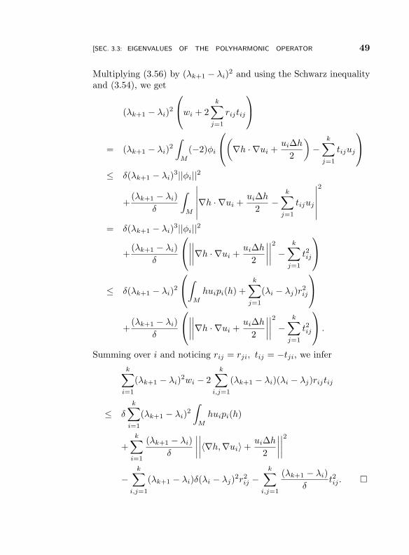
Multiplying (3.56) by (λk+1 − λi)2 and using the Schwarz inequality
and (3.54), we get
(λk+1 − λi)2
wi + 2k∑
j=1
rijtij
= (λk+1 − λi)2
∫
M
(−2)φi
(∇h · ∇ui +
ui∆h
2
)−
k∑
j=1
tijuj
≤ δ(λk+1 − λi)3||φi||2
+(λk+1 − λi)
δ
∫
M
∣∣∣∣∣∣∇h · ∇ui +
ui∆h
2−
k∑
j=1
tijuj
∣∣∣∣∣∣
2
= δ(λk+1 − λi)3||φi||2
+(λk+1 − λi)
δ
∣∣∣∣
∣∣∣∣∇h · ∇ui +ui∆h
2
∣∣∣∣
∣∣∣∣2
−k∑
j=1
t2ij
≤ δ(λk+1 − λi)2
∫
M
huipi(h) +k∑
j=1
(λi − λj)r2ij
+(λk+1 − λi)
δ
∣∣∣∣
∣∣∣∣∇h · ∇ui +ui∆h
2
∣∣∣∣
∣∣∣∣2
−k∑
j=1
t2ij
.
Summing over i and noticing rij = rji, tij = −tji, we infer
k∑
i=1
(λk+1 − λi)2wi − 2
k∑
i,j=1
(λk+1 − λi)(λi − λj)rijtij
≤ δ
k∑
i=1
(λk+1 − λi)2
∫
M
huipi(h)
+
k∑
i=1
(λk+1 − λi)
δ
∣∣∣∣
∣∣∣∣〈∇h,∇ui〉 +ui∆h
2
∣∣∣∣
∣∣∣∣2
−k∑
i,j=1
(λk+1 − λi)δ(λi − λj)2r2ij −
k∑
i,j=1
(λk+1 − λi)
δt2ij .
“eigenvaluecm2013/9/2page 50
i
i
i
i
i
i
i
i
50 [CAP. 3: UNIVERSAL INEQUALITIES FOR EIGENVALUES
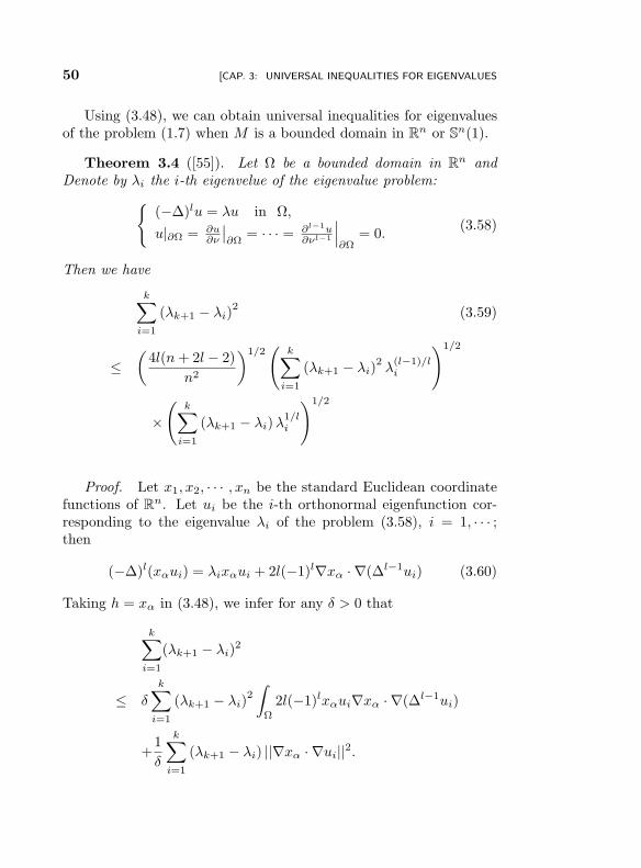
Using (3.48), we can obtain universal inequalities for eigenvaluesof the problem (1.7) when M is a bounded domain in R
n or Sn(1).
Theorem 3.4 ([55]). Let Ω be a bounded domain in Rn and
Denote by λi the i-th eigenvelue of the eigenvalue problem:
(−∆)lu = λu in Ω,
u|∂Ω = ∂u∂ν
∣∣∂Ω
= · · · = ∂l−1u∂νl−1
∣∣∣∂Ω
= 0.(3.58)
Then we have
k∑
i=1
(λk+1 − λi)2
(3.59)
≤(
4l(n+ 2l − 2)
n2
)1/2(
k∑
i=1
(λk+1 − λi)2λ
(l−1)/li
)1/2
×(
k∑
i=1
(λk+1 − λi)λ1/li
)1/2
Proof. Let x1, x2, · · · , xn be the standard Euclidean coordinatefunctions of R
n. Let ui be the i-th orthonormal eigenfunction cor-responding to the eigenvalue λi of the problem (3.58), i = 1, · · · ;then
(−∆)l(xαui) = λixαui + 2l(−1)l∇xα · ∇(∆l−1ui) (3.60)
Taking h = xα in (3.48), we infer for any δ > 0 that
k∑
i=1
(λk+1 − λi)2
≤ δ
k∑
i=1
(λk+1 − λi)2∫
Ω
2l(−1)lxαui∇xα · ∇(∆l−1ui)
+1
δ
k∑
i=1
(λk+1 − λi) ||∇xα · ∇ui||2.
“eigenvaluecm2013/9/2page 51
i
i
i
i
i
i
i
i
[SEC. 3.3: EIGENVALUES OF THE POLYHARMONIC OPERATOR 51
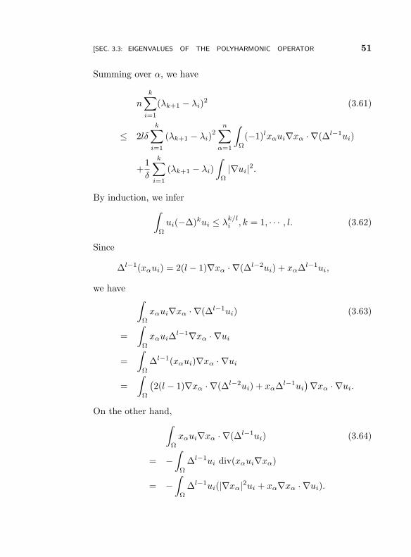
Summing over α, we have
n
k∑
i=1
(λk+1 − λi)2 (3.61)
≤ 2lδ
k∑
i=1
(λk+1 − λi)2
n∑
α=1
∫
Ω
(−1)lxαui∇xα · ∇(∆l−1ui)
+1
δ
k∑
i=1
(λk+1 − λi)
∫
Ω
|∇ui|2.
By induction, we infer
∫
Ω
ui(−∆)kui ≤ λk/li , k = 1, · · · , l. (3.62)
Since
∆l−1(xαui) = 2(l − 1)∇xα · ∇(∆l−2ui) + xα∆l−1ui,
we have∫
Ω
xαui∇xα · ∇(∆l−1ui) (3.63)
=
∫
Ω
xαui∆l−1∇xα · ∇ui
=
∫
Ω
∆l−1(xαui)∇xα · ∇ui
=
∫
Ω
(2(l − 1)∇xα · ∇(∆l−2ui) + xα∆l−1ui
)∇xα · ∇ui.
On the other hand,
∫
Ω
xαui∇xα · ∇(∆l−1ui) (3.64)
= −∫
Ω
∆l−1ui div(xαui∇xα)
= −∫
Ω
∆l−1ui(|∇xα|2ui + xα∇xα · ∇ui).
“eigenvaluecm2013/9/2page 52
i
i
i
i
i
i
i
i
52 [CAP. 3: UNIVERSAL INEQUALITIES FOR EIGENVALUES
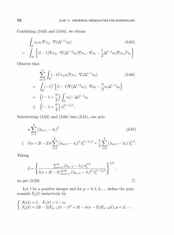
Combining (3.63) and (3.64), we obtain
∫
Ω
xαui∇xα · ∇(∆l−1ui) (3.65)
=
∫
M
(l − 1)∇xα · ∇(∆l−2ui)∇xα · ∇ui −
1
2∆l−1ui|∇xα|2ui
Observe that
n∑
α=1
∫
Ω
(−1)lxαui∇xα · ∇(∆l−1ui) (3.66)
=
∫
Ω
(−1)l
(l − 1)∇(∆l−2ui) · ∇ui −n
2ui∆
l−1ui
=(l − 1 +
n
2
)∫
Ω
ui(−∆)l−1ui
≤(l − 1 +
n
2
)λ
(l−1)/li .
Substituting (3.62) and (3.66) into (3.61), one gets
n
k∑
i=1
(λk+1 − λi)2
(3.67)
≤ l(n+ 2l − 2)δ
k∑
i=1
(λk+1 − λi)2λ
(l−1)/li +
1
δ
k∑
i=1
(λk+1 − λi)λ1/li .
Taking
δ =
∑ki=1 (λk+1 − λi)λ
1/li
l(n+ 2l − 2)∑k
i=1 (λk+1 − λi)2λ
(l−1)/li
1/2
,
we get (3.59).
Let l be a positive integer and for p = 0, 1, 2, ..., define the poly-nomials Fp(t) inductively by
F0(t) = 1, F1(t) = t− n,Fp(t) = (2t− 2)Fp−1(t) − (t2 + 2t− n(n− 2))Fp−2(t), p = 2, · · · .
“eigenvaluecm2013/9/2page 53
i
i
i
i
i
i
i
i
[SEC. 3.3: EIGENVALUES OF THE POLYHARMONIC OPERATOR 53
(3.68)
Set
Fl(t) = tl − al−1tl−1 + · · · + (−1)l−1a1t+ (−n)l. (3.69)
Theorem 3.4 ([55]). Let λi be the i-th eigenvalue of the eigen-value problem:
(−∆)lu = λu in Ω,
u|∂Ω = ∂u∂ν
∣∣∂Ω
= · · · = ∂l−1u∂νl−1
∣∣∣∂Ω
= 0,
where Ω is a compact domain in Sn(1). Then we have
k∑
i=1
(λk+1 − λi)2
(3.70)
≤ 1
n
k∑
i=1
(λk+1 − λi)2(a+
l−1λi
l−1
l + · · · + a+1 λi
1l + a+
0
)1/2
×
k∑
i=1
(λk+1 − λi)(n2 + 4λ
1/2i
)1/2
,
where a+j = max0, aj.
Proof. As before, let x1, x2, · · · , xn+1 be the standard coordinatefunctions of R
n+1; then
Sn(1) = (x1, . . . , xn+1) ∈ R
n+1;
n+1∑
α=1
x2α = 1.
It is well known that
∆xα = −nxα, α = 1, · · · , n+ 1. (3.71)
Taking the Laplacian of the equation∑n+1
α=1 x2α = 1 and using (3.71),
we get
n+1∑
α=1
|∇xα|2 = n. (3.72)
“eigenvaluecm2013/9/2page 54
i
i
i
i
i
i
i
i
54 [CAP. 3: UNIVERSAL INEQUALITIES FOR EIGENVALUES
Let ui be the i-th orthonormal eigenfunction corresponding to theeigenvalue λi, i = 1, 2, · · · . For any δ > 0, by taking h = xα in(3.48), we have
k∑
i=1
(λk+1 − λi)2
∫
Ω
u2i |∇xα|2
≤ δk+1∑
i=1
(λk+1 − λi)2
∫
Ω
xαui((−∆)l(xαui) − λixαui)
+1
δ
k∑
i=1
(λk+1 − λi)
∣∣∣∣
∣∣∣∣∇xα · ∇ui +ui∆xα
2
∣∣∣∣
∣∣∣∣2
Taking sum on α from 1 to n+ 1 and using (3.72), we get
n
k∑
i=1
(λk+1 − λi)2 (3.73)
≤ δ
k+1∑
i=1
(λk+1 − λi)2
n+1∑
α=1
∫
Ω
xαui((−∆)l(xαui) − λixαui)
+1
δ
k∑
i=1
(λk+1 − λi)
n+1∑
α=1
∣∣∣∣
∣∣∣∣∇xα · ∇ui +ui∆xα
2
∣∣∣∣
∣∣∣∣2
.
It is easy to see that
n+1∑
α=1
∣∣∣∣
∣∣∣∣∇xα · ∇ui +ui∆xα
2
∣∣∣∣
∣∣∣∣2
(3.74)
=
∫
Ω
n+1∑
α=1
((∇xα · ∇ui)
2 − n∇xα · ∇uiuixα +n2u2
ix2α
4
)
=n2
4+
∫
Ω
|∇ui|2
≤ n2
4+ λ
1/li .
For any smooth functions f, g on Ω, we have from the Bochner for-
“eigenvaluecm2013/9/2page 55
i
i
i
i
i
i
i
i
[SEC. 3.3: EIGENVALUES OF THE POLYHARMONIC OPERATOR 55
mula that
∆(∇f · ∇g) (3.75)
= 2∇2f · ∇2g + ∇f · ∇(∆g) + ∇g · ∇(∆f)
+2(n− 1)∇f · ∇g,
where
∇2f · ∇2g =n∑
s,t=1
∇2f(es, et)∇2g(es, et),
being e1, · · · , en orthonormal vector fields locally defined on Ω. Since
∇2xα = −xαI,
we infer from (3.75) by taking f = xα that
∆(∇xα · ∇g) (3.76)
= −2xα∆g + ∇xα · ∇(∆g) + (n− 2)∇xα · ∇g= −2xα∆g + ∇xα · ∇((∆ + (n− 2))g).
For each q = 0, 1, · · · , thanks to (3.71) and (3.76), there are polyno-mials Bq and Cq of degrees less than or equal to q such that
∆q(xαg) = xαBq(∆)g + 2∇xα · ∇(Cq(∆)g). (3.77)
It is obvious that
B0 = 1, B1 = t− n, C0 = 0, C1 = 1. (3.78)
It follows from (3.71), (3.76) and (3.77) that
∆q(xαg) = ∆(∆q−1(xαg)) (3.79)
= ∆(xαBq−1(∆)g + 2∇xα · ∇(Cq−1(∆)g))
= xα((∆ − n)Bq−1(∆) − 4∆Cq−1(∆))g
+2∇xα · ∇((Bq−1(∆) + (∆ + (n− 2))Cq−1(∆))g).
Thus, for any q = 2, · · · , we have
Bq(∆) = (∆ − n)Bq−1(∆) − 4∆Cq−1(∆), (3.80)
Cq(∆) = Bq−1(∆) + (∆ + (n− 2))Cq−1(∆). (3.81)
“eigenvaluecm2013/9/2page 56
i
i
i
i
i
i
i
i
56 [CAP. 3: UNIVERSAL INEQUALITIES FOR EIGENVALUES
Consequently,
Bq(∆) (3.82)
= (2∆ − 2)Bq−1(∆) − (∆ + n− 2)Bq−1(∆) − 4∆Cq−1(∆)
= (2∆ − 2)Bq−1(∆) − (∆2 + 2∆ − n(n− 2))Bq−2(∆)
+4∆[Bq−2(∆) + (∆ + n− 2)Cq−2(∆) − Cq−1(∆)]
= (2∆ − 2)Bq−1(∆) − (∆2 + 2∆ − n(n− 2))Bq−2(∆), q = 2, · · · .
Since (3.78) and (3.82) hold, we know that Bq = Fq, ∀q = 0, 1, · · · .It follows from (3.77) and the divergence theorem that
∫
Ω
xαui((−∆)l(xαui) − λixαui) (3.83)
=
∫
Ω
xαui
((−1)l (xαBl(∆)ui + 2∇xα · ∇(Cl(∆)ui)) − λixαui
)
=
∫
Ω
xαui
((−1)l
(xα(∆l − al−1∆
l−1 + · · · + (−n)l)ui
+2∇xα · ∇(Cl(∆)ui)) − λixαui)
=
∫
Ω
(−1)lxαui
(xα(−al−1∆
l−1 + · · · + (−n)l)ui + 2∇xα · ∇(Cl(∆)ui))
Summing on α, one has
∫
Ω
xαui((−∆)l(xαui) − λixαui) (3.84)
=
∫
Ω
ui(−1)l(−al−1∆l−1 + · · · + (−n)la0)ui
= al−1
∫
Ω
ui(−∆)l−1ui + · · · + a1
∫
Ω
ui(−∆)ui + nl
∫
Ω
u2i
≤ a+l−1λ
(l−1)/li + · · · + a+
1 λ1/li + nl.
“eigenvaluecm2013/9/2page 57
i
i
i
i
i
i
i
i
[SEC. 3.4: EIGENVALUES OF THE BUCKLING PROBLEM 57
Substituting (3.74) and (3.84) into (3.73), we infer
n
k∑
i=1
(λk+1 − λi)2
≤ δ
k∑
i=1
(λk+1 − λi)2(a+
l−1λ(l−1)/li + · · · + a+
1 λ1/li + nl)
+1
δ
k∑
i=1
(λk+1 − λi)
(λ
1/li +
n2
4
).
Taking
δ =
∑ki=1(λk+1 − λi)
(λ
1/li + n2
4
)
∑ki=1(λk+1 − λi)2(a
+l−1λ
(l−1)/li + · · · + a+
1 λ1/li + nl)
1/2
,
we get (3.70).
3.4 Eigenvalues of the Buckling Problem
Let Ω ⊂ Rn and consider the problem
∆2u = −λ∆u,u|∂Ω = ∂u
∂ν
∣∣∂Ω
= 0(3.85)
which is used to describe the critical buckling load of a clamped platesubjected to a uniform compressive force around its boundary.
Payne, Polya and Weinberger [77] proved
λ2/λ1 < 3 for Ω ⊂ R2.
For Ω ⊂ Rn this reads
λ2/λ1 < 1 + 4/n.
Subsequently Hile and Yeh [51] reconsidered this problem obtainingthe improved bound
λ2
λ1≤ n2 + 8n+ 20
(n+ 2)2for Ω ⊂ R
n.
“eigenvaluecmb”2013/9/2page 58
i
i
i
i
i
i
i
i
58 [CAP. 3: UNIVERSAL INEQUALITIES FOR EIGENVALUES
Ashbaugh [3] proved :
n∑
i=1
λi+1 ≤ (n+ 4)λ1. (3.86)
This inequality has been improved to the following form [54]:
n∑
i=1
λi+1 +4(λ2 − λ1)
n+ 4≤ (n+ 4)λ1.
Cheng and Yang introduced a new method to construct trial functionsfor the problem (3.85) and obtained the following universal inequality[28]:
k∑
i=1
(λk+1 − λi)2 ≤ 4(n+ 2)
n2
k∑
i=1
(λk+1 − λi)λi. (3.87)
It has been proved in [88] that for the problem (1.5) ifM is a boundedconnected domain in an n-dimensional unit sphere, then the followinginequality holds
2k∑
i=1
(λk+1 − λi)2 (3.88)
≤k∑
i=1
(λk+1 − λi)2
(δλi +
δ2(λi − (n− 2))
4(δλi + n− 2)
)
+1
δ
k∑
i=1
(λk+1 − λi)
(λi +
(n− 2)2
4
),
where δ is any positive constant.The inequality (3.87) has been generalized to eigenvalues of buck-
ling problem of arbitrary orders. That is, we have
Theorem 3.5 ([54]). Let l ≥ 2 and let λi be the i-th eigenvalueof the following eigenvalue problem:
(−∆)lu = −λ∆u in Ω,
u|∂Ω = ∂u∂ν
∣∣∂Ω
= · · · = ∂l−1u∂νl−1
∣∣∣∂Ω
= 0.(3.89)
“eigenvaluecm2013/9/2page 59
i
i
i
i
i
i
i
i
[SEC. 3.4: EIGENVALUES OF THE BUCKLING PROBLEM 59
where Ω is a bounded domain with smooth boundary in Rn. Then for
k = 1, · · · , we have
k∑
i=1
(λk+1 − λi)2 (3.90)
≤ 2(2l2 + (n− 4)l + 2 − n)1/2
n
k∑
i=1
(λk+1 − λi)2λ
(l−2)/(l−1)i
1/2
×
k∑
i=1
(λk+1 − λi)λ1/(l−1)i
1/2
.
Before proving theorem 3.5, let us recall a method of constructingtrial functions developed by Cheng-Yang (Cf. [28], [54]). LetM be ann-dimensional complete submanifold in an m-dimensional Euclideanspace R
m. Denote by · the canonical metric on Rm as well as that
induced on M . Let ∆ and ∇ be the Laplacian and the gradientoperator of M , respectively. Let Ω be a bounded connected domainof M with smooth boundary ∂Ω and let ν be the outward unit normalvector field of ∂Ω. For functions f and g on Ω, the Dirichlet innerproduct (f, g)D of f and g is given by
(f, g)D =
∫
Ω
∇f · ∇g.
The Dirichlet norm of a function f is defined by
||f ||D = (f, f)D1/2 =
(∫
Ω
|∇f |2)1/2
.
Consider the eigenvalue problem
(−∆)lu = −λ∆u in Ω,
u|∂Ω = ∂u∂ν
∣∣∂Ω
= · · · = ∂l−1u∂νl−1
∣∣∣∂Ω
= 0.(3.91)
Let
0 < λ1 ≤ λ2 ≤ λ3 ≤ · · · ,
“eigenvaluecm2013/9/2page 60
i
i
i
i
i
i
i
i
60 [CAP. 3: UNIVERSAL INEQUALITIES FOR EIGENVALUES
denote the successive eigenvalues, where each eigenvalue is repeatedaccording to its multiplicity.
Let ui be the i-th orthonormal eigenfunction of the problem (3.91)corresponding to the eigenvalue λi, i = 1, 2, · · · , that is, ui satisfies
(−∆)lui = −λi∆ui in Ω,
ui|∂Ω = ∂ui
∂ν
∣∣∂Ω
= · · · ∂l−1u∂νl−1
∣∣∣∂Ω
= 0,
(ui, uj)D =∫Ω〈∇ui,∇uj〉 = δij , ∀ i, j.
(3.92)
For k = 1, · · · , l, let ∇k denote the k-th covariant derivative operatoron M , defined in the usual weak sense via an integration by partsformula. For a function f on Ω, the squared norm of ∇kf is definedas
∣∣∇kf∣∣2 =
n∑
i1,··· ,ik=1
(∇kf(ei1 , · · · , eik
))2, (3.93)
where e1, · · · , en are orthonormal vector fields locally defined on Ω.Define the Sobolev space H2
l (Ω) by
H2l (Ω) = f : f, |∇f |, · · · ,
∣∣∇lf∣∣ ∈ L2(Ω).
Then H2l (Ω) is a Hilbert space with respect to the norm || · ||l,2:
||f ||l,2 =
(∫
Ω
(l∑
k=0
|∇kf |2))1/2
. (3.94)
Consider the subspace H2l,D(Ω) of H2
l (Ω) defined by
H2l,D(Ω) =
f ∈ H2
l (Ω) : f |∂Ω =∂f
∂ν
∣∣∣∣∂Ω
= · · · ∂l−1u
∂νl−1
∣∣∣∣∂Ω
= 0
.
The operator (−∆)l defines a self-adjoint operator acting on H2l,D(Ω)
with discrete eigenvalues 0 < λ1 ≤ · · · ≤ λk ≤ · · · for the bucklingproblem (3.91) and the eigenfunctions ui∞i=1 defined in (3.92) forma complete orthonormal basis for the Hilbert space H2
l,D(Ω). If φ ∈H2
l,D(Ω) satisfies (φ, uj)D = 0, ∀j = 1, 2, · · · , k, then the Rayleigh-Ritz inequality tells us that
λk+1||φ||2D ≤∫
Ω
φ(−∆)lφ. (3.95)
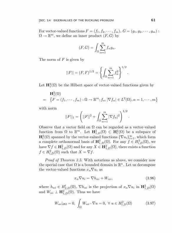
“eigenvaluecm2013/9/2page 61
i
i
i
i
i
i
i
i
[SEC. 3.4: EIGENVALUES OF THE BUCKLING PROBLEM 61
For vector-valued functions F = (f1, f2, · · · , fm), G = (g1, g2, · · · , gm) :Ω → R
m, we define an inner product (F,G) by
(F,G) =
∫
Ω
m∑
α=1
fαgα.
The norm of F is given by
||F || = (F, F )1/2 =
∫
Ω
m∑
α=1
f2α
1/2
.
Let H21(Ω) be the Hilbert space of vector-valued functions given by
H21(Ω)
=F = (f1, · · · , fm) : Ω → R
m; fα, |∇fα| ∈ L2(Ω), α = 1, · · · ,m
with norm
||F ||1 =
(||F ||2 +
∫
Ω
m∑
α=1
|∇fα|2)1/2
.
Observe that a vector field on Ω can be regarded as a vector-valuedfunction from Ω to R
m. Let H21,D(Ω) ⊂ H2
l (Ω) be a subspace of
H2l (Ω) spanned by the vector-valued functions ∇ui∞i=1, which form
a complete orthonormal basis of H21,D(Ω). For any f ∈ H2
l,D(Ω), we
have ∇f ∈ H21,D(Ω) and for anyX ∈ H2
1,D(Ω), there exists a function
f ∈ H2l,D(Ω) such that X = ∇f .
Proof of Theorem 3.5. With notations as above, we consider nowthe special case that Ω is a bounded domain in R
n. Let us decomposethe vector-valued functions xα∇ui as
xα∇ui = ∇hαi +Wαi, (3.96)
where hαi ∈ H l2,D(Ω), ∇hαi is the projection of xα∇ui in H2
1,D(Ω)
and Wαi ⊥ H21,D(Ω). Thus we have
Wαi|∂Ω = 0,
∫
Ω
Wαi · ∇u = 0, ∀ u ∈ H2l,D(Ω) (3.97)
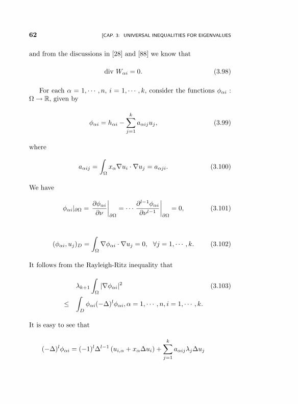
“eigenvaluecm2013/9/2page 62
i
i
i
i
i
i
i
i
62 [CAP. 3: UNIVERSAL INEQUALITIES FOR EIGENVALUES
and from the discussions in [28] and [88] we know that
div Wαi = 0. (3.98)
For each α = 1, · · · , n, i = 1, · · · , k, consider the functions φαi :Ω → R, given by
φαi = hαi −k∑
j=1
aαijuj , (3.99)
where
aαij =
∫
Ω
xα∇ui · ∇uj = aαji. (3.100)
We have
φαi|∂Ω =∂φαi
∂ν
∣∣∣∣∂Ω
= · · · ∂l−1φαi
∂νl−1
∣∣∣∣∂Ω
= 0, (3.101)
(φαi, uj)D =
∫
Ω
∇φαi · ∇uj = 0, ∀j = 1, · · · , k. (3.102)
It follows from the Rayleigh-Ritz inequality that
λk+1
∫
Ω
|∇φαi|2 (3.103)
≤∫
D
φαi(−∆)lφαi, α = 1, · · · , n, i = 1, · · · , k.
It is easy to see that
(−∆)lφαi = (−1)l∆l−1 (ui,α + xα∆ui) +
k∑
j=1
aαijλj∆uj
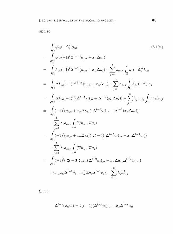
“eigenvaluecm2013/9/2page 63
i
i
i
i
i
i
i
i
[SEC. 3.4: EIGENVALUES OF THE BUCKLING PROBLEM 63
and so
∫
Ω
φαi(−∆)lφαi (3.104)
=
∫
Ω
φαi(−1)l∆l−1 (ui,α + xα∆ui)
=
∫
Ω
hαi(−1)l∆l−1 (ui,α + xα∆ui) −k∑
j=1
aαij
∫
Ω
uj(−∆)lhαi
=
∫
Ω
∆hαi(−1)l∆l−2 (ui,α + xα∆ui) −k∑
j=1
aαij
∫
Ω
hαi(−∆)luj
=
∫
Ω
∆hαi(−1)l((∆l−2ui),α + ∆l−2(xα∆ui)) +k∑
j=1
λjaαij
∫
Ω
hαi∆uj
=
∫
Ω
(−1)l(ui,α + xα∆ui)((∆l−2ui),α + ∆l−2(xα∆ui))
−k∑
j=1
λjaαij
∫
Ω
〈∇hαi,∇uj〉
=
∫
Ω
(−1)l(ui,α + xα∆ui)((2l − 3)(∆l−2ui),α + xα∆l−1ui))
−k∑
j=1
λjaαij
∫
Ω
〈∇hαi,∇uj〉
=
∫
Ω
(−1)l((2l − 3)ui,α(∆l−2ui),α + xα∆ui(∆l−2ui),α)
+ui,αxα∆l−1ui + x2α∆ui∆
l−1ui −k∑
j=1
λja2αij
Since
∆l−1(xαui) = 2(l − 1)(∆l−2ui),α + xα∆l−1ui,
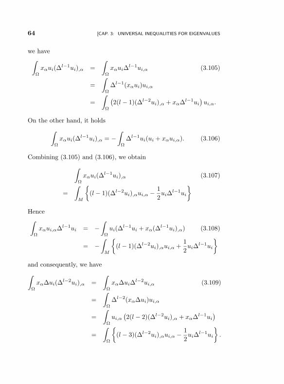
“eigenvaluecm2013/9/2page 64
i
i
i
i
i
i
i
i
64 [CAP. 3: UNIVERSAL INEQUALITIES FOR EIGENVALUES
we have∫
Ω
xαui(∆l−1ui),α =
∫
Ω
xαui∆l−1ui,α (3.105)
=
∫
Ω
∆l−1(xαui)ui,α
=
∫
Ω
(2(l − 1)(∆l−2ui),α + xα∆l−1ui
)ui,α.
On the other hand, it holds
∫
Ω
xαui(∆l−1ui),α = −
∫
Ω
∆l−1ui(ui + xαui,α). (3.106)
Combining (3.105) and (3.106), we obtain
∫
Ω
xαui(∆l−1ui),α (3.107)
=
∫
M
(l − 1)(∆l−2ui),αui,α − 1
2ui∆
l−1ui
Hence∫
Ω
xαui,α∆l−1ui = −∫
Ω
ui(∆l−1ui + xα(∆l−1ui),α) (3.108)
= −∫
M
(l − 1)(∆l−2ui),αui,α +
1
2ui∆
l−1ui
and consequently, we have
∫
Ω
xα∆ui(∆l−2ui),α =
∫
Ω
xα∆ui∆l−2ui,α (3.109)
=
∫
Ω
∆l−2(xα∆ui)ui,α
=
∫
Ω
ui,α
(2(l − 2)(∆l−2ui),α + xα∆l−1ui
)
=
∫
Ω
(l − 3)(∆l−2ui),αui,α − 1
2ui∆
l−1ui
.
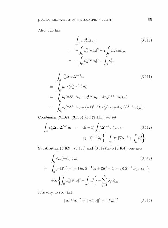
“eigenvaluecm2013/9/2page 65
i
i
i
i
i
i
i
i
[SEC. 3.4: EIGENVALUES OF THE BUCKLING PROBLEM 65
Also, one has∫
Ω
uix2α∆ui (3.110)
= −∫
Ω
x2α|∇ui|2 − 2
∫
Ω
xαuiui,α
= −∫
Ω
x2α|∇ui|2 +
∫
Ω
u2i ,
∫
Ω
x2α∆ui∆
l−1ui (3.111)
=
∫
Ω
ui∆(x2α∆l−1ui)
=
∫
Ω
ui(2∆l−1ui + x2α∆lui + 4xα(∆l−1ui),α)
=
∫
Ω
ui(2∆l−1ui + (−1)l−1λix2α∆ui + 4xα(∆l−1ui),α).
Combining (3.107), (3.110) and (3.111), we get
∫
Ω
x2α∆ui∆
l−1ui = 4(l − 1)
∫
Ω
(∆l−2ui),αui,α (3.112)
+(−1)l−1λi
−∫
Ω
x2α|∇ui|2 +
∫
Ω
u2i
.
Substituting (3.109), (3.111) and (3.112) into (3.104), one gets
∫
Ω
φαi(−∆)lφαi (3.113)
=
∫
Ω
(−1)l(−l + 1)ui∆
l−1ui + (2l2 − 4l + 3)(∆l−2ui),αui,α
+λi
∫
Ω
x2α|∇ui|2 −
∫
Ω
u2i
−
k∑
j=1
λja2αij .
It is easy to see that
||xα∇ui||2 = ||∇hαi||2 + ||Wαi||2 (3.114)
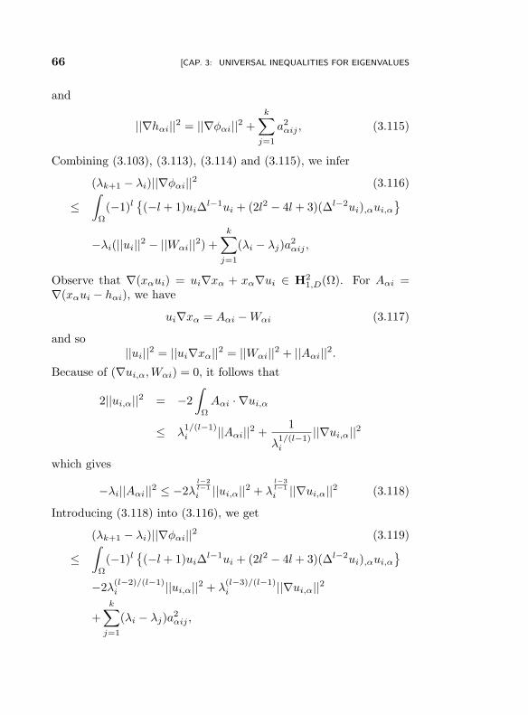
“eigenvaluecm2013/9/2page 66
i
i
i
i
i
i
i
i
66 [CAP. 3: UNIVERSAL INEQUALITIES FOR EIGENVALUES
and
||∇hαi||2 = ||∇φαi||2 +
k∑
j=1
a2αij , (3.115)
Combining (3.103), (3.113), (3.114) and (3.115), we infer
(λk+1 − λi)||∇φαi||2 (3.116)
≤∫
Ω
(−1)l(−l + 1)ui∆
l−1ui + (2l2 − 4l + 3)(∆l−2ui),αui,α
−λi(||ui||2 − ||Wαi||2) +
k∑
j=1
(λi − λj)a2αij ,
Observe that ∇(xαui) = ui∇xα + xα∇ui ∈ H21,D(Ω). For Aαi =
∇(xαui − hαi), we have
ui∇xα = Aαi −Wαi (3.117)
and so||ui||2 = ||ui∇xα||2 = ||Wαi||2 + ||Aαi||2.
Because of (∇ui,α,Wαi) = 0, it follows that
2||ui,α||2 = −2
∫
Ω
Aαi · ∇ui,α
≤ λ1/(l−1)i ||Aαi||2 +
1
λ1/(l−1)i
||∇ui,α||2
which gives
−λi||Aαi||2 ≤ −2λl−2
l−1
i ||ui,α||2 + λl−3
l−1
i ||∇ui,α||2 (3.118)
Introducing (3.118) into (3.116), we get
(λk+1 − λi)||∇φαi||2 (3.119)
≤∫
Ω
(−1)l(−l + 1)ui∆
l−1ui + (2l2 − 4l + 3)(∆l−2ui),αui,α
−2λ(l−2)/(l−1)i ||ui,α||2 + λ
(l−3)/(l−1)i ||∇ui,α||2
+
k∑
j=1
(λi − λj)a2αij ,
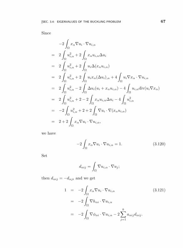
“eigenvaluecm2013/9/2page 67
i
i
i
i
i
i
i
i
[SEC. 3.4: EIGENVALUES OF THE BUCKLING PROBLEM 67
Since
−2
∫
Ω
xα∇ui · ∇ui,α
= 2
∫
Ω
u2i,α + 2
∫
Ω
xαui,α∆ui
= 2
∫
Ω
u2i,α + 2
∫
Ω
ui∆(xαui,α)
= 2
∫
Ω
u2i,α + 2
∫
Ω
uixα(∆ui),α + 4
∫
Ω
ui∇xα · ∇ui,α
= 2
∫
Ω
u2i,α − 2
∫
Ω
∆ui(ui + xαui,α) − 4
∫
Ω
ui,αdiv(ui∇xα)
= 2
∫
Ω
u2i,α + 2 − 2
∫
Ω
xαui,α∆ui − 4
∫
Ω
u2i,α
= −2
∫
Ω
u2i,α + 2 + 2
∫
Ω
∇ui · ∇(xαui,α)
= 2 + 2
∫
Ω
xα∇ui · ∇ui,α,
we have
−2
∫
Ω
xα∇ui · ∇ui,α = 1. (3.120)
Set
dαij =
∫
Ω
∇ui,α · ∇uj ;
then dαij = −dαji and we get
1 = −2
∫
Ω
xα∇ui · ∇ui,α (3.121)
= −2
∫
Ω
∇hαi · ∇ui,α
= −2
∫
Ω
∇φαi · ∇ui,α − 2
k∑
j=1
aαijdαij .
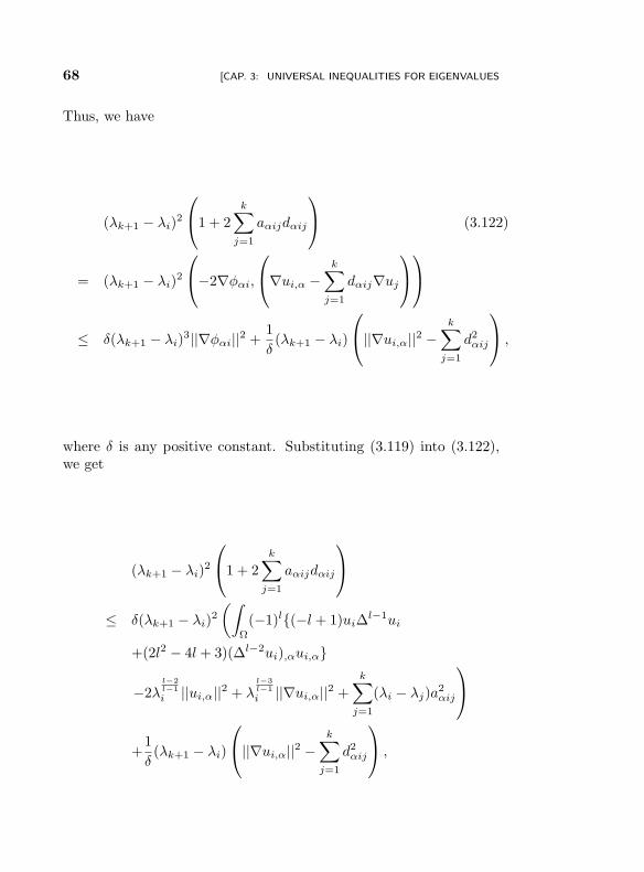
“eigenvaluecm2013/9/2page 68
i
i
i
i
i
i
i
i
68 [CAP. 3: UNIVERSAL INEQUALITIES FOR EIGENVALUES
Thus, we have
(λk+1 − λi)2
1 + 2
k∑
j=1
aαijdαij
(3.122)
= (λk+1 − λi)2
−2∇φαi,
∇ui,α −k∑
j=1
dαij∇uj
≤ δ(λk+1 − λi)3||∇φαi||2 +
1
δ(λk+1 − λi)
||∇ui,α||2 −k∑
j=1
d2αij
,
where δ is any positive constant. Substituting (3.119) into (3.122),we get
(λk+1 − λi)2
1 + 2
k∑
j=1
aαijdαij
≤ δ(λk+1 − λi)2
(∫
Ω
(−1)l(−l + 1)ui∆l−1ui
+(2l2 − 4l + 3)(∆l−2ui),αui,α
−2λl−2
l−1
i ||ui,α||2 + λl−3
l−1
i ||∇ui,α||2 +
k∑
j=1
(λi − λj)a2αij
+1
δ(λk+1 − λi)
||∇ui,α||2 −k∑
j=1
d2αij
,
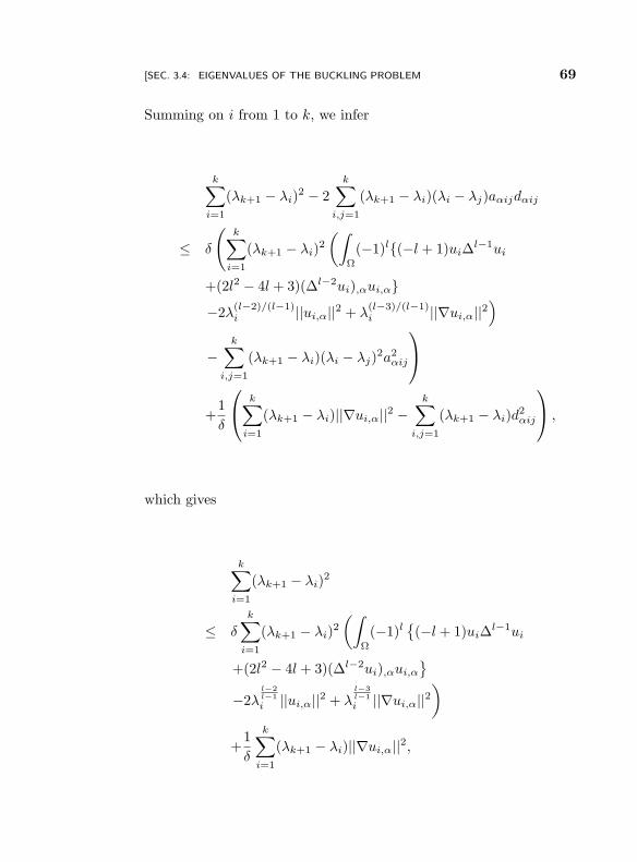
“eigenvaluecm2013/9/2page 69
i
i
i
i
i
i
i
i
[SEC. 3.4: EIGENVALUES OF THE BUCKLING PROBLEM 69
Summing on i from 1 to k, we infer
k∑
i=1
(λk+1 − λi)2 − 2
k∑
i,j=1
(λk+1 − λi)(λi − λj)aαijdαij
≤ δ
(k∑
i=1
(λk+1 − λi)2
(∫
Ω
(−1)l(−l + 1)ui∆l−1ui
+(2l2 − 4l + 3)(∆l−2ui),αui,α−2λ
(l−2)/(l−1)i ||ui,α||2 + λ
(l−3)/(l−1)i ||∇ui,α||2
)
−k∑
i,j=1
(λk+1 − λi)(λi − λj)2a2
αij
+1
δ
k∑
i=1
(λk+1 − λi)||∇ui,α||2 −k∑
i,j=1
(λk+1 − λi)d2αij
,
which gives
k∑
i=1
(λk+1 − λi)2
≤ δ
k∑
i=1
(λk+1 − λi)2
(∫
Ω
(−1)l(−l + 1)ui∆
l−1ui
+(2l2 − 4l + 3)(∆l−2ui),αui,α
−2λl−2
l−1
i ||ui,α||2 + λl−3
l−1
i ||∇ui,α||2)
+1
δ
k∑
i=1
(λk+1 − λi)||∇ui,α||2,
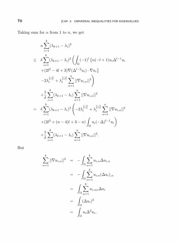
“eigenvaluecm2013/9/2page 70
i
i
i
i
i
i
i
i
70 [CAP. 3: UNIVERSAL INEQUALITIES FOR EIGENVALUES
Taking sum for α from 1 to n, we get
nk∑
i=1
(λk+1 − λi)2
≤ δ
k∑
i=1
(λk+1 − λi)2
(∫
Ω
(−1)ln(−l + 1)ui∆
l−1ui
+(2l2 − 4l + 3)∇(∆l−2ui) · ∇ui
−2λl−2
l−1
i + λl−3
l−1
i
n∑
α=1
||∇ui,α||2)
+1
δ
k∑
i=1
(λk+1 − λi)n∑
α=1
||∇ui,α||2
= δk∑
i=1
(λk+1 − λi)2
(−2λ
l−2
l−1
i + λl−3
l−1
i
n∑
α=1
||∇ui,α||2
+(2l2 + (n− 4)l + 3 − n)
∫
Ω
ui(−∆)l−1ui
)
+1
δ
k∑
i=1
(λk+1 − λi)
n∑
α=1
||∇ui,α||2.
But
k∑
α=1
||∇ui,α||2 = −∫
Ω
k∑
α=1
ui,α∆ui,α
= −∫
Ω
k∑
α=1
ui,α(∆ui),α
=
∫
Ω
k∑
α=1
ui,αα∆ui
=
∫
Ω
(∆ui)2
=
∫
Ω
ui∆2ui,
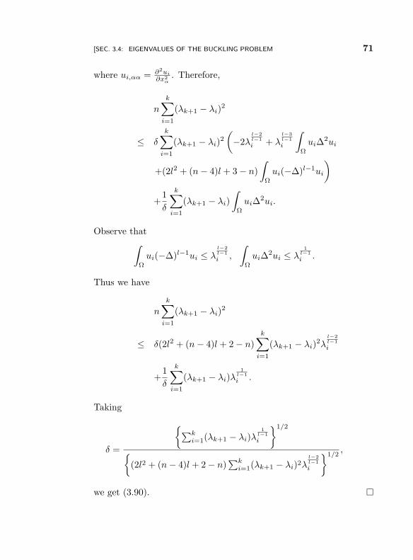
“eigenvaluecm2013/9/2page 71
i
i
i
i
i
i
i
i
[SEC. 3.4: EIGENVALUES OF THE BUCKLING PROBLEM 71
where ui,αα = ∂2ui
∂x2α
. Therefore,
nk∑
i=1
(λk+1 − λi)2
≤ δk∑
i=1
(λk+1 − λi)2
(−2λ
l−2
l−1
i + λl−3
l−1
i
∫
Ω
ui∆2ui
+(2l2 + (n− 4)l + 3 − n)
∫
Ω
ui(−∆)l−1ui
)
+1
δ
k∑
i=1
(λk+1 − λi)
∫
Ω
ui∆2ui.
Observe that∫
Ω
ui(−∆)l−1ui ≤ λl−2
l−1
i ,
∫
Ω
ui∆2ui ≤ λ
1l−1
i .
Thus we have
n
k∑
i=1
(λk+1 − λi)2
≤ δ(2l2 + (n− 4)l + 2 − n)k∑
i=1
(λk+1 − λi)2λ
l−2
l−1
i
+1
δ
k∑
i=1
(λk+1 − λi)λ1
l−1
i .
Taking
δ =
∑ki=1(λk+1 − λi)λ
1l−1
i
1/2
(2l2 + (n− 4)l + 2 − n)
∑ki=1(λk+1 − λi)2λ
l−2
l−1
i
1/2,
we get (3.90).
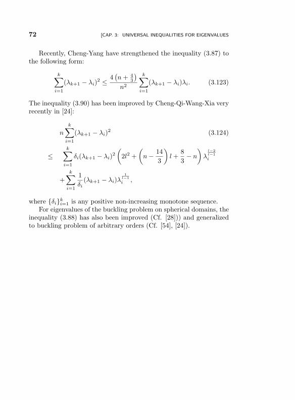
“eigenvaluecm2013/9/2page 72
i
i
i
i
i
i
i
i
72 [CAP. 3: UNIVERSAL INEQUALITIES FOR EIGENVALUES
Recently, Cheng-Yang have strengthened the inequality (3.87) tothe following form:
k∑
i=1
(λk+1 − λi)2 ≤ 4
(n+ 4
3
)
n2
k∑
i=1
(λk+1 − λi)λi. (3.123)
The inequality (3.90) has been improved by Cheng-Qi-Wang-Xia veryrecently in [24]:
n
k∑
i=1
(λk+1 − λi)2 (3.124)
≤k∑
i=1
δi(λk+1 − λi)2
(2l2 +
(n− 14
3
)l +
8
3− n
)λ
l−2
l−1
i
+
k∑
i=1
1
δi(λk+1 − λi)λ
1l−1
i ,
where δiki=1 is any positive non-increasing monotone sequence.
For eigenvalues of the buckling problem on spherical domains, theinequality (3.88) has also been improved (Cf. [28])) and generalizedto buckling problem of arbitrary orders (Cf. [54], [24]).
“eigenvaluecm2013/9/2page 73
i
i
i
i
i
i
i
i
Chapter 4
Polya Conjecture and
Related Results
4.1 Introduction
Let Ω ⊂ Rn be a bounded open set and consider the eigenvalue
problem of the Dirichlet Laplacian on Ω:
∆u+ λu = 0 in Ω,u|∂Ω = 0.
(4.1)
In 1960, Polya [81] showed that for any “plane covering domain” Ωin R
2 (those that tile R2) the Weyl asymptotic relation (1.) is in fact
a one-sided inequality (his proof also works for Rn-covering domains)
and conjectured, for any bounded domain Ω ⊂ Rn, the inequality
λk ≥ C(n)
(k
|Ω|
)2/n
∀k, with C(n) =(2π)2
ω2nn
. (4.2)
Polya’s conjecture has been a central problem about eigenvalues andmany important developments have been made during the past years.In 1982, Li-Yau [72] showed the lower bound
k∑
i=1
λi ≥nkC(n)
n+ 2
(k
|Ω|
)2/n
(4.3)
73
“eigenvaluecm2013/9/2page 74
i
i
i
i
i
i
i
i
74 [CAP. 4: POLYA CONJECTURE AND RELATED RESULTS
which yields an individual lower bound on λk in the form
λk ≥ nC(n)
n+ 2
(k
|Ω|
)2/n
. (4.4)
Similar bounds for eigenvalues with Neumann boundary conditionshave been proved in [62], [63] and [65]. It was pointed out in [66]that (4.3) also follows from an earlier result by Berezin [11] by theLegendre transformation. The inequality (4.3) has been improved byMelas:
Theorem 4.1 ([75]). For any bounded domain Ω ⊂ Rn and any
k ≥ 1, the eigenvalues of the problem (4.1) satisfy the inequality
k∑
i=1
λi ≥nkC(n)
n+ 2
(k
|Ω|
)2/n
+ d(n)k|Ω|I(Ω)
(4.5)
where the constant dn depends only on the dimension and I(Ω) =mina∈Rn
∫Ω|x− a|2dx is the “moment of inertia” of Ω.
Proof. Fix a k ≥ 1 and let u1, · · · , uk be an orthonormal setof eigenfunctions of (4.1) corresponding to the set of eigenvaluesλ1, · · · , λk. We consider the Fourier transform of each eigenfunction
fj(ξ) = uj(ξ) = (2π)−n/2
∫
Ω
uj(x)eix·ξdx. (4.6)
¿From Plancherel’s Theorem, we know that f1, · · · , fk is an orthonor-mal set in R
n. Bessel’s inequality implies that for every ξ ∈ Rn
k∑
j=1
|fj(ξ)|2 ≤ (2π)−n
∫
Ω
|eix·ξ|dx = (2π)−n|Ω| (4.7)
and
k∑
j=1
|∇fj(ξ)|2 ≤ (2π)−n
∫
Ω
|ixeix·ξ|dx = (2π)−nI(Ω). (4.8)
Since uj |∂Ω = 0 it is easy to see that∫
Rn
|ξ|2|fj(ξ)|2dξ =
∫
Ω
|∇uj |2 = λj . (4.9)
“eigenvaluecm2013/9/2page 75
i
i
i
i
i
i
i
i
[SEC. 4.1: INTRODUCTION 75
Setting
F (ξ) =
k∑
j=1
|fj(ξ)|2; (4.10)
then 0 ≤ F (ξ) ≤ (2π)−n|Ω|,
|∇F (ξ)| ≤ 2(
k∑
j=1
|fj(ξ)|2)1/2(
k∑
j=1
|∇fj(ξ)|2)1/2 (4.11)
≤ 2(2π)−n√
|Ω|I(Ω), ∀ξ ∈ Rn,
∫
Rn
F (ξ)dξ = k (4.12)
and
∫
Rn
|ξ|2F (ξ)dξ =k∑
j=1
λj . (4.13)
Let F ∗(ξ) = φ(|ξ|) denote the decreasing radial rearrangement of F .By approximating F we may assume that the function φ : [0;+∞) →[0, (2π)−n|Ω|] is absolutely continuous. Setting µ(t) = |F ∗ > t| =|F > t| the co-area formula (1.17) implies that
µ(t) =
∫ (2π)−n|Ω|
t
∫
F=s|∇F |−1dσsds. (4.14)
Observe that F ∗ is radial and so µ(φ(s)) = |F ∗ > φ(s)| = ωnsn
which gives nωnsn−1 = µ′(φ(s))φ′(s) a.e. It follows from (4.11),
(4.14) and the isoperimetric inequality that
−µ′(φ(s)) =
∫
F=φ(s)|∇F |−1dσs (4.15)
≥ ρ−1|F = φ(s)|≥ ρ−1nωns
n−1
“eigenvaluecm2013/9/2page 76
i
i
i
i
i
i
i
i
76 [CAP. 4: POLYA CONJECTURE AND RELATED RESULTS
and so for almost every s
−ρ ≤ φ′(s) ≤ 0, (4.16)
where
ρ = 2(2π)−n√|Ω|I(Ω).
From (4.12) and (4.13), we have
k =
∫
Rn
F (ξ)dξ =
∫
Rn
F ∗(ξ)dξ (4.17)
= nωn
∫ ∞
0
sn−1φ(s)ds
and
k∑
j=1
λj =
∫
Rn
|xi|2F (ξ)dξ (4.18)
≥∫
Rn
|xi|2F ∗(ξ)dξ
= nωn
∫ ∞
0
sn+1φ(s)ds.
We need an elementary lemma.
Lemma 4.1([75]) Let n ≥ 1, ρ, A > 0 and ψ : [0,+∞) → [0,+∞)be decreasing (and absolutely continuous) such that
−ρ ≤ φ′(s) ≤ 0,
∫ ∞
0
sn−1ψ(s)ds = A. (4.19)
Then∫ ∞
0
sn+1ψ(s)ds ≥ 1
n+ 2(nA)
n+2
n ψ(0)−2n +
Aψ(0)2
6(n+ 2)ρ2. (4.20)
Applying Lemma 4.1 to the function φ with A = (nωn)−1k, ρ =2(2π)−n
√|Ω|I(Ω) we get in view of (4.12) and (4.13) that
∑
j=1
λj ≥ n
n+ 2ω− 2
nn k
n+2
n φ(0)−2n +
ckφ(0)2
(n+ 2)ρ2(4.21)
“eigenvaluecmb”2013/9/2page 77
i
i
i
i
i
i
i
i
[SEC. 4.2: THE KROGER’S THEOREM 77
where c is any constant such that 0 < c < 16 . Observe that 0 <
φ(0) ≤ (2π)−n|Ω| and that if R is such that ωnRn = |Ω|, then I(Ω) ≥∫
B(R)|x|2dx = nωnRn+2
n+2 and so
ρ ≥ 2(2π)−n
√n
n+ 2ω− 2
nn |Ω|n+2
n +1 (4.22)
≥ (2π)−nω− 1
nn |Ω|n+1
n .
Let us choose c independent of n satisfying c < (2π)2ω− 1
nn . It is easy
to see that the function
g(t) =n
n+ 2ω− 2
nn k
n+2
n t−2t +
ckt2
(n+ 2)ρ2
is decreasing on (0, (2π)−n|Ω|]. We can replace φ(0) by (2π)−n|Ω| in(4.21) which gives the inequality (4.5).
4.2 The Kroger’s Theorem
Let λk be the kth eigenvalue for the Neumann boundary value prob-lem with respect to the Laplace operator on a bounded domainwith piecewise smooth boundary in R
n. Polys conjecture states that
λk ≤ Cn
(k|Ω|
) 2n
. With respect to this conjecture, Kroger proved the
following result.
Theorem 4.2 ([62]). The first k+1 Neumann eigenvalues of a abounded domain Ω with piecewise smooth boundary in R
n satisfy theinequality
λk+1 ≤ infr>2π
(nk
αn−1|Ω|
)1/n
rn+2
n+2 (αn−1|Ω|) − (2π)n∑k
j=1 λj
rn
n αn−1|Ω| − (2π)nk(4.24)
where αn−1 denotes the area of the (n− 1)-unit sphere in Rn.
Taking
r = 2π
(n(k + 1)
αn−1|Ω|
)1/n
,
“eigenvaluecm2013/9/2page 78
i
i
i
i
i
i
i
i
78 [CAP. 4: POLYA CONJECTURE AND RELATED RESULTS
one gets
Corollary 4.1. Under the assumptions of the Theorem the fol-lowing inequality holds for every k:
k∑
j=1
λj ≤ n
n+ 2(2π)2
(1
nαn−1|Ω|
)− 2n
kn+2
n (4.25)
Proof of Theorem 4.2. Let φjkj=1 be the set of orthonormal
eigenfunctions for the eigenvalues λ1, ..., λk. Fix z ∈ Rn and consider
hz : R → C given by hz(y) = eiy·z. Letting aj =∫Ωhz(x)uj(x)dx;
then the projection of hz(y) ≡ eiz·y into the subspace of L2(Ω)spanned by φ1, ..., φk can be written as
hz(y)|spanuiki=1
=
k∑
j=1
(∫
Ω
hz(x)uj(x)dx
)uj(y) (4.26)
=k∑
j=1
ajuj(y).
It is clear that the function gz(y) ≡ hz(y) −∑k
j=1 ajuj(y) is orthog-onal to uj , j = 1, · · · , k. Thus we have
λk+1 ≤∫Ω|∇gz(y)|2dy∫
Ωg2
zdy. (4.27)
Elementary computation sows that
∫
Ω
|∇gz(y)|2dy = |z|2|Ω| −k∑
j=1
|aj |2λj (4.28)
and
∫
Ω
g2zdy = |Ω| −
k∑
j=1
|aj |2. (4.29)
“eigenvaluecm2013/9/2page 79
i
i
i
i
i
i
i
i
[SEC. 4.2: THE KROGER’S THEOREM 79
Assuming that r > 2π(
nkαn−1|Ω|
)1/n
; then
λk+1 ≤∫
Br
(∫Ω|∇gz(y)|2dy
)dz
∫Br
(∫Ωgz(y)2dy
)dz
(4.30)
Since∫
Br
(∫
Ω
|∇gz(y)|2dy)dz (4.31)
=
∫
Br
|z|2|Ω|dz −∫
Br
k∑
j=1
λj |aj |2dz
=rn+2αn−1|Ω|
n+ 2−
k∑
j=1
λj
∫
Br
|aj |2dz
and∫
Br
(∫
Ω
(gz(y))2dy
)dz (4.32)
=
∫
Br
|Ω|dz −∫
Br
k∑
j=1
|aj |2dz
=rnαn−1|Ω|
n−
k∑
j=1
∫
Br
|aj |2dz,
we get
λk+1 ≤rn+2αn−1|Ω|
n+2 −∑kj=1 λj
∫Br
|aj |2dzrnαn−1|Ω|
n −∑kj=1
∫Br
|aj |2dz. (4.33)
Recall that the Fourier transform uj of uj is given by
uj(z) = (2π)−n2
∫
Rn
eiy·zuj(y)dy
and we know from the Plancherel Theorem that∫
Rn |uj |2(z)dz =
“eigenvaluecm2013/9/2page 80
i
i
i
i
i
i
i
i
80 [CAP. 4: POLYA CONJECTURE AND RELATED RESULTS
∫Rn |uj |2(y)dy. Hence we have
∫
Br
∣∣∣∣∫
Ω
hzujdy
∣∣∣∣2
dz ≤∫
Rn
∣∣∣∣∫
Ω
hzujdy
∣∣∣∣2
dz
= (2π)n
∫
Rn
|uj(z)|2dz
= (2π)n
∫
Rn
|uj(y)|2dy
= (2π)n.
Let us prove by induction that
λk+1 ≤rn+2αn−1|Ω|
n+2 − (2π)n∑k
j=1 λj
rnαn−1|Ω|n − (2π)nk
. (4.34)
Suppose that (4.34) is true for k − 1, that is
λk ≤rn+2αn−1|Ω|
n+2 − (2π)n∑k−1
j=1 λj
rnαn−1|Ω|n − (2π)n(k − 1)
.
We then have that
λk ≤rn+2αn−1|Ω|
n+2 − (2π)n∑k
j=1 λj
rnαn−1|Ω|n − (2π)nk
=A
B,
where
A =rn+2αn−1|Ω|
n+ 2− (2π)n
k∑
j=1
λj
and
B =rnαn−1|Ω|
n− (2π)nk.
Setting Cl = (2π)n −∫
Br|al|2dz and observing
rnαn−1|Ω|n
− (2π)nk > 0,
“eigenvaluecm2013/9/2page 81
i
i
i
i
i
i
i
i
[SEC. 4.3: A GENERALIZED POLYA CONJECTURE BY CHENG-YANG 81
we get
λk+1 ≤ A+∑k
l=1 λlCl
B +∑k
l=1 Cl
≤ A+ λk
∑kl=1 Cl
B +∑k
l=1 Cl
≤ A+ AB
∑kl=1 Cl
B +∑k
l=1 Cl
=A
B.
This completes the proof of Theorem 4.2.
4.3 A generalized Polya conjecture by
Cheng-Yang
In [31], Cheng-Yang investigated eigenvalues of the Dirichlet Lapla-cian on a bounded domain in an n-dimensional complete Riemannianmanifold M and proposed a generalized Polya conjecture.
Cheng-Yang’s Conjecture ([31]). Let Ω be a bounded domainin an n-dimensional complete Riemannian manifold M . Then, thereexists a constant c(M,Ω), which only depends on M and Ω such thateigenvalue λi’s of the eigenvalue problem
∆u = −λu in Ω,u|∂Ω = 0.
(4.35)
satisfy
1
k
k∑
i=1
λi + c(M,Ω) ≥ n
n+ 2
4π2
(ωn|Ω|) 2n
k2n , k = 1, · · · , (4.36)
λi + c(M,Ω) ≥ 4π2
(ωn|Ω|) 2n
k2n , k = 1, · · · , (4.37)
“eigenvaluecmb”2013/9/2page 82
i
i
i
i
i
i
i
i
82 [CAP. 4: POLYA CONJECTURE AND RELATED RESULTS
Remark 4.1. Cheng-Yang believed that in the above conjecture,
whenM is the unit sphere Sn(1), c(M,Ω) = n2
4 , whenM is the hyper-
bolic space Hn(−1), c(M,Ω) = − (n−1)2
4 and when M is a completeminimal submanifold in R
N , c(M,Ω) = 0. Cheng-Yang obtained apartial solution to the above conjecture.
Theorem 4.3 ([31]). Let Ω be a bounded domain in an n-dimensionalcomplete Riemannian manifold M . Then, there exists a constantH2 > 0, which only depends on M and Ω such that eigenvalue λ′is ofthe problem (4.35) satisfy
1
k
k∑
i=1
λi +H20 ≥ n√
(n+ 2)(n+ 4)
4π2
(ωn|Ω|) 2n
k2n , k = 1, · · · , (4.38)
Moreover, when M is the unit sphere Sn(1), one can take H2
0 = n2
4and when M is a complete minimal submanifold in R
N , one can takeH2
0 = 0.
A crucial result in the proof of Theorem 4.3 is the following
Lemma 4.2 ([25]). Let µ1 ≤ · · · ≤ µk+1 be any non-negative realnumbers satisfying
k∑
i=1
(µk+1 − µi)2 ≤ 4
t
k∑
i=1
µi(µk+1 − µi). (4.39)
Define
Gk =1
k
k∑
i=1
µi, Tk =1
k
k∑
i=1
µ2i , Fk =
(1 +
2
t
)G2
k − Tk. (4.40)
Then, we have
Fk+1 ≤ C(t, k)
(k + 1
k
) 4t
Fk, (4.41)
“eigenvaluecm2013/9/2page 83
i
i
i
i
i
i
i
i
[SEC. 4.3: A GENERALIZED POLYA CONJECTURE BY CHENG-YANG 83
where t is any positive real number and
C(t, k) = 1 − 1
3t
(k
k + 1
) 4t(1 + 2
t
) (1 + 4
t
)
(k + 1)3< 1. (4.42)
Proof of Theorem 4.3. From Nashs theorem, we know that M canbe isometricly immersed into a Euclidean space R
N , that is, thereexists an isometric immersion:
φ : M → RN . (4.43)
Thus, M can be seen as a complete submanifold isometricly immersedinto R
N . We denote by |H| the mean curvature of the immersion φ.From (3.16), we have
k∑
i=1
(λk+1 − λi)2 ≤ 4
n
k∑
i=1
(λk+1 − λi)(λi +n2
4supΩ
|H|2). (4.44)
Since eigenvalues are invariants of isometries, the above inequalityholds for any isometric immersion from M into a Euclidean space.Let us define
Φ = φ;φ is an isometric immersion from M into a Euclidean space.
Putting
H0 = infφ∈Φ
supΩ
|H|2;
then
k∑
i=1
(λk+1 − λi)2 ≤ 4
n
k∑
i=1
(λk+1 − λi)(λi +n2
4H2
0 ). (4.45)
Letting µi = λi + n2
4 H20 ; then
k∑
i=1
(µk+1 − µi)2 ≤ 4
n
k∑
i=1
µi(µk+1 − µi). (4.46)
“eigenvaluecm2013/9/2page 84
i
i
i
i
i
i
i
i
84 [CAP. 4: POLYA CONJECTURE AND RELATED RESULTS
From theorem 2.1 with t = n of [25], we have
Fk+1 ≤ C(n, k)
(k + 1
k
) 1n
Fk ≤(k + 1
k
) 1n
Fk.
Therefore, we infer
Fk+1
(k + 1)4n
≤ Fk
k4n
.
For any positive integers l and k, we have
Fk+l
(k + l)4n
≤ Fk
k4n
.
From the Weyl’s asymptotic formula (1.10)
liml→∞
λl
l2n
=4π2
(ωn|Ω|) 2n
,
we get
liml→∞
1λl
∑li=1 λi
l2n
=n
n+ 2
4π2
(ωn|Ω|) 2n
and
liml→∞
1λl
∑li=1 λ
2i
l4n
=n
n+ 4
16π4
(ωn|Ω|) 4n
.
Hence
liml→∞
Fk+l
(k + l)4n
=2n
(n+ 2)(n+ 4)
16π4
(ωn|Ω|) 4n
.
According to (4.46), we have, for any positive integer k,
Fk
k4n
≥ 2n
(n+ 2)(n+ 4)
16π4
(ωn|Ω|) 4n
. (4.47)
“eigenvaluecmb”2013/9/2page 85
i
i
i
i
i
i
i
i
[SEC. 4.4: ANOTHER GENERALIZED POLYA CONJECTURE 85
Since
Fk =
(1 +
2
n
)G2
k − Tk ≤ 2
nG2
k,
we get
2
n
G2k
k4n
≥ Fk
k4n
≥ 2n
(n+ 2)(n+ 4)
16π4
(ωn|Ω|) 4n
which implies (4.38).In order to finish the proof of Theorem 4.3, we need only to ob-
serve that Sn(1) can be seen as a compact hypersurface in R
n+1 withmean curvature 1 and that a complete minimal submanifold in R
N
has mean curvature |H| = 0.
4.4 Another generalized Polya conjecture
Let Ω be a bounded domain in Rn and let L be the elliptic operator
of order 2t defined by
Lu =t∑
m=r+1
am−r(−∆)mu, u ∈ C∞(Ω)
where r ≥ 0 is an integer, am−r’s are constants with am−r ≥ 0, r+1 ≤m ≤ t, at−r = 1, t a fixed positive integer. Consider the followingeigenvalue problem about L which is important in the study of variousbranches of mathematics, such as differential equations, differentialgeometry and mathematical physics:
Lu = λ(−∆)ru, u ∈ C∞(Ω),
(∂/∂ν)ju|∂Ω = 0, j = 0, 1, 2, · · · , t− 1.(4.48)
Let
0 < λ1,r ≤ λ2,r ≤ · · · ≤ λk,r ≤ · · · → ∞. (4.49)
be the eigenvalues of the problem (4.48). In [58], the following con-jecture was proposed :
“eigenvaluecmb”2013/9/2page 86
i
i
i
i
i
i
i
i
86 [CAP. 4: POLYA CONJECTURE AND RELATED RESULTS
Generalized Polya Conjecture. The eigenvalues λk,r, k =1, 2, · · · , of the eigenvalue problem (1.7) of the operator L satisfiesthe inequality
λk,r ≥t−r∑
m=1
amCm
(k
|Ω|
)2m/n
. (4.50)
With respect to the above generalized Polya conjecture, Ku-Ku-Tang showed in [58] that if r is even, then
λk,r ≥t−r∑
m=1
nam
n+ 2mCm
(k
|Ω|
)2m/n
, k = 1, 2, · · · . (4.51)
This section provides comparison theorems between the k-th eigenval-ues of the problem (4.1) and that of the problem (4.48) which showsthat if the Polya conjecture (4.2) is true then so is the generalizedPolya conjecture (4.50).
Theorem 4.3 ([93]). Let M be an n(≥ 2)-dimensional compactRiemannian manifold with boundary. Denote by ∆ the Laplacianoperator on M and let L be the elliptic operator given by
Lu =
t∑
m=r+1
am−r(−∆)mu, u ∈ C∞(M), (4.52)
where r ≥ 0 is an integer, am−r’s are constants with am−r ≥ 0, r +1 ≤ m ≤ t, at−r = 1, t a fixed positive integer. Consider the follow-ing eigenvalue problems:
Lu = λ(−∆)ru, u ∈ C∞(M),
(∂/∂ν)ju|∂M = 0, j = 0, 1, 2, · · · , t− 1,(4.53)
(−∆)r+1u = Λ(−∆)ru, u ∈ C∞(M),
(∂/∂ν)ju|∂M = 0, j = 0, 1, 2, · · · , r, (4.54)
−∆u = λu in M,u|∂M = 0.
(4.55)
“eigenvaluecm2013/9/2page 87
i
i
i
i
i
i
i
i
[SEC. 4.4: ANOTHER GENERALIZED POLYA CONJECTURE 87
Denote by
0 < λ1,r ≤ λ2,r ≤ · · · → ∞ (4.56)
0 < Λ1,r ≤ Λ2,r ≤ · · · → ∞ (4.57)
and
0 < λ1 < λ2 ≤ · · · → ∞ (4.58)
the successive eigenvalues for (4.53), (4.54) and (4.55), respectively.Here each eigenvalue is repeated according to its multiplicity. Thenfor any k = 1, 2, · · · , we have
λk,r ≥ a1Λk,r + a2Λ2k,r + · · · + at−(r+1)Λ
t−(r+1)k,r + Λt−r
k,r (4.59)
and
Λk,r ≥ λk. (4.60)
Remark 1.1. If M is a bounded domain in Rn, we know from
the inequality
λk,r ≥ a1λk + a2λ2k + · · · + at−(r+1)λ
t−(r+1)k + λt−r
k (4.61)
which is a combination of (4.59) and (4.60) that if the Polya conjec-ture (4.2) is true then so is the generalized Polya conjecture (4.50).
Proof of Theorem 4.3. Let uiki=1 be a set of orthonormal eigen-
functions of the problem (4.53) corresponding to λi,rki=1, that is,
Lui = λi,r(−∆)rui, in M,
ui|∂M = · · · = ∂t−1ui
∂νt−1
∣∣∣∂M
= 0,∫
Mui(−∆)ruj = δij , i, j = 1, · · · , k.
Similarly, let viki=1 be a set of orthonormal eigenfunctions of the
problem (4.54) corresponding to Λi,rki=1, that is,
(−∆)r+1vi = Λi,r(−∆)rvi in M,
vi|∂M = · · · = ∂rvi
∂νr
∣∣∣∂M
= 0,∫
Mvi(−∆)rvj = δij , i, j = 1, · · · , k.
“eigenvaluecm2013/9/2page 88
i
i
i
i
i
i
i
i
88 [CAP. 4: POLYA CONJECTURE AND RELATED RESULTS
Let w =∑k
j=1 αjuj 6= 0 be such that
∫
M
w(−∆)rvj = 0, ∀j = 1, · · · , k − 1. (4.62)
Such an element w exists because αj |1 ≤ j ≤ k is a non-trivialsolution of a system of (k − 1)-linear equations
k∑
j=1
αj
∫
M
uj(−∆)rvi = 0, 1 ≤ i ≤ k − 1, (4.63)
in k unknowns. Notice that if u ∈ C∞(M) satisfies
u|∂M =∂u
∂ν
∣∣∣∣∂M
= · · · =∂t−1u
∂νt−1
∣∣∣∣∂M
= 0,
then
u|∂M = ∇u|∂M = ∆u|∂M = ∇(∆u)|∂M = · · · =
= ∆p−1u∣∣∂M
= ∇(∆p−1u)∣∣∂M
= 0, when t = 2p
and
u|∂M = ∇u|∂M = ∆u|∂M = ∇(∆u)|∂M = · · · = ∆k−1u∣∣∂M
= ∇(∆p−1u)∣∣∂M
= ∆pu|∂M = 0, when t = 2p+ 1.
Observe that∫
Mw(−∆)rw 6= 0. In fact, from divergence theorem,
we have
∫
M
w(−∆)rw =
∫M
(∆r/2w)2, if r is even,∫M
∣∣∇(∆(r−1)/2w)∣∣2 , if r is odd.
Thus, if∫
Mw(−∆)rw = 0, then ∆r/2w = 0 when r is even and
∆(r−1)/2w = 0 when r is odd. It then follows from the maximumprinciple for harmonic functions that ∆r/2−1w = 0 when r is even and∆(r−1)/2−1w = 0 when r is odd. Continuing this process, we concludethat w = 0. This is a contradiction. Thus
∫Mw(−∆)rw 6= 0. Let us
assume without loss of generality that∫
M
w(−∆)rw = 1. (4.64)
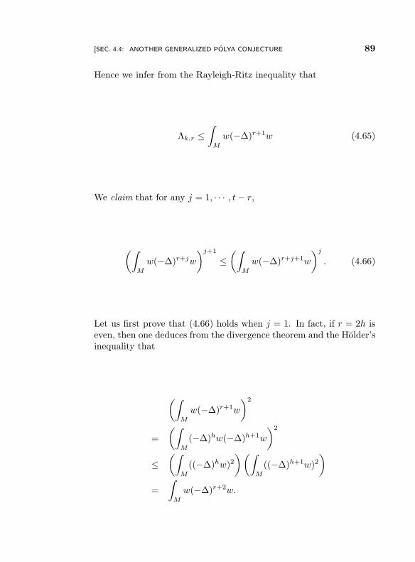
“eigenvaluecm2013/9/2page 89
i
i
i
i
i
i
i
i
[SEC. 4.4: ANOTHER GENERALIZED POLYA CONJECTURE 89
Hence we infer from the Rayleigh-Ritz inequality that
Λk,r ≤∫
M
w(−∆)r+1w (4.65)
We claim that for any j = 1, · · · , t− r,
(∫
M
w(−∆)r+jw
)j+1
≤(∫
M
w(−∆)r+j+1w
)j
. (4.66)
Let us first prove that (4.66) holds when j = 1. In fact, if r = 2h iseven, then one deduces from the divergence theorem and the Holder’sinequality that
(∫
M
w(−∆)r+1w
)2
=
(∫
M
(−∆)hw(−∆)h+1w
)2
≤(∫
M
((−∆)hw)2)(∫
M
((−∆)h+1w)2)
=
∫
M
w(−∆)r+2w.
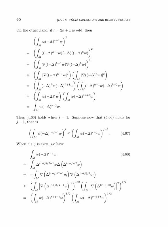
“eigenvaluecm2013/9/2page 90
i
i
i
i
i
i
i
i
90 [CAP. 4: POLYA CONJECTURE AND RELATED RESULTS
On the other hand, if r = 2h+ 1 is odd, then
(∫
M
w(−∆)r+1w
)2
=
(∫
M
((−∆)h+1w)(−∆)((−∆)hw)
)2
=
(∫
M
∇((−∆)h+1w)∇((−∆)hw)
)2
≤(∫
M
|∇((−∆)h+1w|2)(∫
M
|∇((−∆)hw)|2)
=
(∫
M
(−∆)hw(−∆)h+1w
)(∫
M
(−∆)h+1w(−∆)h+2w
)
=
(∫
M
w(−∆)rw
)(∫
M
w(−∆)2h+3w
)
=
∫
M
w(−∆)r+2w.
Thus (4.66) holds when j = 1. Suppose now that (4.66) holds forj − 1, that is
(∫
M
w(−∆)r+j−1w
)j
≤(∫
M
w(−∆)r+jw
)j−1
. (4.67)
When r + j is even, we have
∫
M
w(−∆)r+jw (4.68)
=
∫
M
∆(r+j)/2−1w∆(∆(r+j)/2w
)
= −∫
M
∇(∆(r+j)/2−1ui
)∇(∆(r+j)/2ui
)
≤(∫
M
∣∣∣∇(∆(r+j)/2−1w
)∣∣∣2)1/2(∫
M
∣∣∣∇(∆(r+j)/2w
)∣∣∣2)1/2
=
(∫
M
w(−∆)r+j−1w
)1/2(∫
M
w(−∆)r+j+1w
)1/2
,
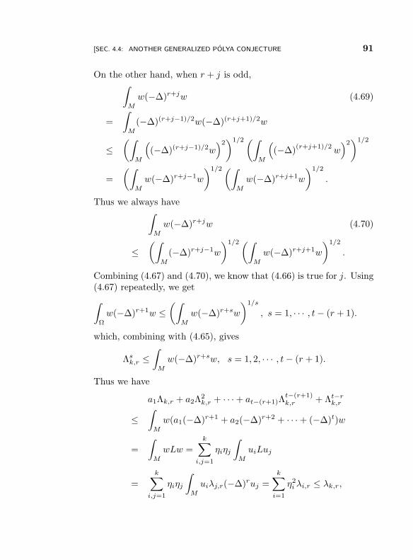
“eigenvaluecm2013/9/2page 91
i
i
i
i
i
i
i
i
[SEC. 4.4: ANOTHER GENERALIZED POLYA CONJECTURE 91
On the other hand, when r + j is odd,∫
M
w(−∆)r+jw (4.69)
=
∫
M
(−∆)(r+j−1)/2w(−∆)(r+j+1)/2w
≤(∫
M
((−∆)(r+j−1)/2w
)2)1/2(∫
M
((−∆)
(r+j+1)/2w)2)1/2
=
(∫
M
w(−∆)r+j−1w
)1/2(∫
M
w(−∆)r+j+1w
)1/2
.
Thus we always have∫
M
w(−∆)r+jw (4.70)
≤(∫
M
(−∆)r+j−1w
)1/2(∫
M
w(−∆)r+j+1w
)1/2
.
Combining (4.67) and (4.70), we know that (4.66) is true for j. Using(4.67) repeatedly, we get
∫
Ω
w(−∆)r+1w ≤(∫
M
w(−∆)r+sw
)1/s
, s = 1, · · · , t− (r + 1).
which, combining with (4.65), gives
Λsk,r ≤
∫
M
w(−∆)r+sw, s = 1, 2, · · · , t− (r + 1).
Thus we have
a1Λk,r + a2Λ2k,r + · · · + at−(r+1)Λ
t−(r+1)k,r + Λt−r
k,r
≤∫
M
w(a1(−∆)r+1 + a2(−∆)r+2 + · · · + (−∆)t)w
=
∫
M
wLw =k∑
i,j=1
ηiηj
∫
M
uiLuj
=
k∑
i,j=1
ηiηj
∫
M
uiλj,r(−∆)ruj =
k∑
i=1
η2i λi,r ≤ λk,r,
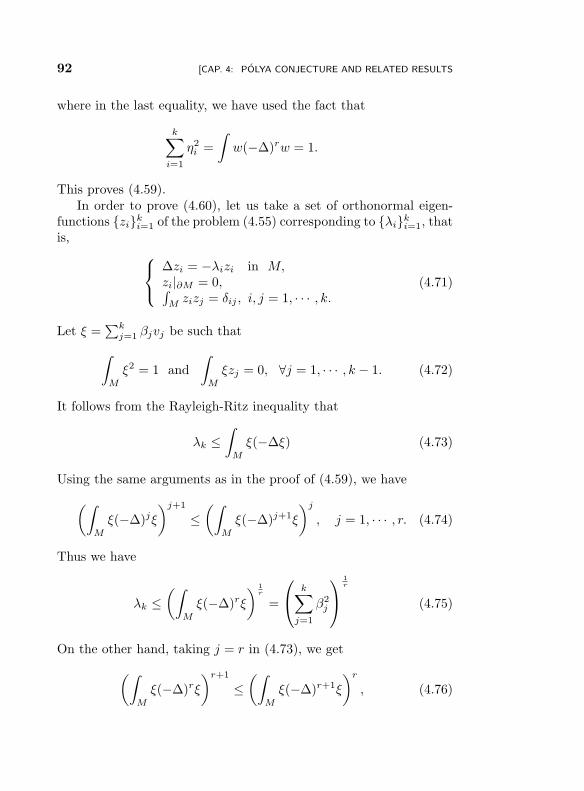
“eigenvaluecm2013/9/2page 92
i
i
i
i
i
i
i
i
92 [CAP. 4: POLYA CONJECTURE AND RELATED RESULTS
where in the last equality, we have used the fact that
k∑
i=1
η2i =
∫w(−∆)rw = 1.
This proves (4.59).In order to prove (4.60), let us take a set of orthonormal eigen-
functions ziki=1 of the problem (4.55) corresponding to λik
i=1, thatis,
∆zi = −λizi in M,zi|∂M = 0,∫
Mzizj = δij , i, j = 1, · · · , k.
(4.71)
Let ξ =∑k
j=1 βjvj be such that
∫
M
ξ2 = 1 and
∫
M
ξzj = 0, ∀j = 1, · · · , k − 1. (4.72)
It follows from the Rayleigh-Ritz inequality that
λk ≤∫
M
ξ(−∆ξ) (4.73)
Using the same arguments as in the proof of (4.59), we have
(∫
M
ξ(−∆)jξ
)j+1
≤(∫
M
ξ(−∆)j+1ξ
)j
, j = 1, · · · , r. (4.74)
Thus we have
λk ≤(∫
M
ξ(−∆)rξ
) 1r
=
k∑
j=1
β2j
1r
(4.75)
On the other hand, taking j = r in (4.73), we get
(∫
M
ξ(−∆)rξ
)r+1
≤(∫
M
ξ(−∆)r+1ξ
)r
, (4.76)
“eigenvaluecm2013/9/2page 93
i
i
i
i
i
i
i
i
[SEC. 4.4: ANOTHER GENERALIZED POLYA CONJECTURE 93
which implies that
k∑
j=1
β2j ≤
(∫
M
ξ(−∆)r+1ξ
) rr+1
(4.77)
=
∫
M
k∑
i,j=1
βiβjvi(−∆)r+1vj
rr+1
=
∫
M
k∑
i,j=1
βiβjviΛj,r(−∆)rvj
rr+1
=
k∑
j=1
Λj,rβ2j
rr+1
≤ Λr
r+1
k,r
k∑
j=1
β2j
rr+1
.
Thus we have
k∑
j=1
β2j ≤ Λr
k,r. (4.78)
Combining (4.75) and (4.78), one gets (4.60).
“eigenvaluecm2013/9/2page 94
i
i
i
i
i
i
i
i
Chapter 5
The Steklov eigenvalue
problems
5.1 Introduction
LetM be an n-dimensional compact Riemannian manifold with bound-ary. The Stekloff problem is to find a solution of the equation
∆u = 0 in M,∂u∂ν = pu on ∂M,
(5.1)
where p is a real number. This problem was first introduced bySteklov for bounded domains in the plane in [87]. His motivationcame from physics. The function u represents the steady state tem-perature on M such that the flux on the boundary is proportionalto the temperature. Problem (5.1) is also important in conductivityand harmonic analysis as it was initially studied by Calderon (Cf.[15]). This connection arises because the set of eigenvalues for theSteklov problem is the same as the set of eigenvalues of the well-known Dirichlet-Neumann map. This map associates to each func-tion u defined on the boundary ∂M , the normal derivative of theharmonic function on M with boundary data u. The Steklov eigen-value problem has appeared in quite a few physical fields, such asfluid mechanics, electromagnetism, elasticity, etc., and received in-
94
“eigenvaluecm2013/9/2page 95
i
i
i
i
i
i
i
i
[SEC. 5.2: ESTIMATES FOR THE STEKLOV EIGENVALUES 95
creasing attention [53], [64]. It has applications, for instance, in theinvestigation of surface waves [12], the analysis of stability of me-chanical oscillators immersed in a viscous fluid [32], and the study ofthe vibration modes of a structure in contact with an incompressiblefluid [13]. Numerical methods have been developed for this prob-lem. For instance, its optimal error estimates of linear finite elementapproximations have been obtained in [2]. Interesting estimates foreigenvalues of the Steklov problem have been obtained some of whichwill be introduced in this chapter.
5.2 Estimates for the Steklov eigenvalues
In this section, we prove some estimates for the Steklov eigenvalues.Let us recall firstly the Reilly’s formula. Let M be n-dimensionalcompact manifold M with boundary ∂M . We denote by 〈, 〉 theRiemannian metric on M as well as that induced on ∂M . Let ∇ and∆ be the connection and the Laplacian on M , respectively. Let νbe the unit outward normal vector of ∂M . The shape operator of∂M is given by S(X) = ∇Xν and the second fundamental form of∂M is defined as II(X,Y ) = 〈S(X), Y 〉, here X,Y ∈ T∂M . Theeigenvalues of S are called the principal curvatures of ∂M and themean curvature H of ∂M is given by H = 1
n−1 tr S, here tr S denotesthe trace of S. For a smooth function f defined on an n-dimensionalcompact manifold M with boundary ∂M , the following identity holds
if u = ∂f∂ν
∣∣∣∂M
, z = f |∂M and Ric denotes the Ricci tencor of M , then
(see [82], p. 46):∫
M
((∆f)2 − |∇2f |2 − Ric(∇f,∇f)
)(5.2)
=
∫
∂M
(((n− 1)Hu+ 2∆z)u+ II(∇z,∇z)
).
Here ∇2f is the Hessian of f ; ∆ and ∇ represent the Laplacianand the gradient on ∂M with respect to the induced metric on ∂M ,respectively.
Theorem 5.1 ([35]). Let M be an n-dimensional compact con-nected Riemannian manifold with non-negative Ricci curvature and
“eigenvaluecm2013/9/2page 96
i
i
i
i
i
i
i
i
96 [CAP. 5: THE STEKLOV EIGENVALUE PROBLEMS
boundary. Assume that the principal curvatures of ∂M are boundedfrom below by a positive constant c. Then the first non-zero eigen-value of the problem (5.1) satisfies p1 >
c2 .
Proof. Let f be the first eigenfunction of the Steklov problem(5.1). Setting z = f |∂M , u = ∂u
∂ν
∣∣∂M
and using Reilly’s formula wefind after integration by parts that
0 > −∫
M
|∇2f |2 ≥ −2
∫
∂M
∇z · ∇u+ c
∫
∂M
|∇z|2.
0 > −2p1
∫
∂M
|∇z|2 + c
∫
∂M
|∇z|2. (5.3)
Since z 6= constant, otherwise f=constant on M which is a contra-diction, we have
∫
∂M
|∇z|2 > 0. (5.4)
Thus (5.3) implies that p1 > c/2.
In view of Theorem 5.1, Escobar conjectured that under the sameconditions as in Theorem 5.1, p1 ≥ c.
Theorem 5.2. Let the conditions be as in Theorem 5.1. Thenwe have
i) The non-zero eigenvalue of the Laplacian of ∂M satisfies
λ1 ≥ (n− 1)c2 (5.5)
with equality holding if and only if M is isometric to a ball of radius1/c in R
n([102]).ii) The non-zero eigenvalue of the Steklov problem (5.1) satisfies
p1 ≤√λ1
(n− 1)c
(√λ1 +
√λ1 − (n− 1)c2
)(5.6)
Moreover, the equality holds in (5.6) if and only if M is isometric toa ball of radius 1/c in R
n ([89]).
“eigenvaluecm2013/9/2page 97
i
i
i
i
i
i
i
i
[SEC. 5.2: ESTIMATES FOR THE STEKLOV EIGENVALUES 97
Proof. Let z be an eigenfunction corresponding to the first nonzeroeigenvalue λ1 of the Laplacian of ∂M :
∆z + λ1z = 0.
Let f in C∞(M) be the solution of the Dirichlet problem
∆f = 0 in M,f |∂M = z.
(5.7)
It then follows from (5.2) and the nonnegativity of the Ricci curvatureof M that
0 ≥∫
M
((∆f)2 − |∇2f |2 − Ric(∇f,∇f)
)(5.8)
=
∫
∂M
(((n− 1)Hh+ 2∆z)h+ II(∇z,∇z)
)
≥∫
∂M
(−2(−λ1z)u+ (n− 1)cu2 + c|∇z|2)
≥∫
∂M
(2λ1zu+ (n− 1)cu2 + cλ1z2)
≥∫
∂M
(n− 1)c
(u+
λ1z
(n− 1)c
)2
+
(cλ1 −
λ21
(n− 1)c
)z2
≥∫
∂M
(cλ1 −
λ21
(n− 1)c
)z2
.
Thus we have
cλ1 −λ2
1
(n− 1)c≤ 0
or
λ1 ≥ (n− 1)c2.
If M is isometric to an n-dimensional Euclidean ball of radius 1c , it is
well known that λ1(M) = (n− 1)c2. Now we assume conversely thatλ1(M) = (n − 1)c2. In this case the inequalities in (5.8) must takeequality sign. In particular, we have
∇2f = 0, H = c, u = − λ1z
(n− 1)c= −cz. (5.9)
“eigenvaluecm2013/9/2page 98
i
i
i
i
i
i
i
i
98 [CAP. 5: THE STEKLOV EIGENVALUE PROBLEMS
From ∇2f = 0, we know that |∇f |2 is a constant and is not zerosince f is not a constant. Without loss of generality, we can assume|∇f |2 = 1. Thus for any point p ∈M , we have
1 = |∇f |2(p) = |∇z2|(p) + u2(p). (5.10)
It follows from (5.10) by integration and u = −cz, that
A(∂M) =
∫
∂M
(|∇z|2 + u2) (5.11)
=
∫
∂M
(λ1z2 + u2)
=
∫
∂M
(nu2).
On the other hand, from
1
2∆(f2) = |∇f |2 + f∆f = 1 (5.12)
and the divergence theorem we have
V (M) =
∫
M
1
2∆(f2) = −
∫
∂M
zu =
∫
∂M
u2
c,
which, combining with (5.11), gives
H = c =1
n· A(∂M)
V (M). (5.13)
It then follows from a result in [83] that M is isometric to a ball inR
n. Since λ1(∂M) = (n − 1)c2, the radius of M is easily seen to be1c . This proves item i) of Theorem 5.1.
Now let us prove (5.6). Let f and z be as in the proof of item i).We have from the Rayleigh-Ritz inequality that (Cf. [59])
p1 ≤∫
∂Mh2
∫M
|∇f |2 (5.14)
and
p1 ≤∫
M|∇f |2∫
∂Mz2
, (5.15)
“eigenvaluecm2013/9/2page 99
i
i
i
i
i
i
i
i
[SEC. 5.2: ESTIMATES FOR THE STEKLOV EIGENVALUES 99
which gives
p21 ≤
∫∂M
h2
∫∂M
z2. (5.16)
It then follows by substituting f into the Reilly’s formula that
0 ≥∫
M
((∆f)2 − |∇2f |2 − Ric(∇f,∇f)
)(5.17)
≥ (n− 1)c
∫
∂M
h2 − 2λ1
∫
∂M
hz + c
∫
∂M
|∇z|2
= (n− 1)c
∫
∂M
h2 − 2λ1
∫
∂M
hz + cλ1
∫
∂M
z2
≥ (n− 1)c
∫
∂M
h2 − 2λ1
(∫
∂M
h2
) 12(∫
∂M
z2
) 12
+ cλ1
∫
∂M
z2.
Hence, we have
(∫
∂M
h2
) 12
≤√λ1
(n− 1)c
(√λ1 +
√λ1 − (n− 1)c2
)(∫
∂M
z2
) 12
.
Hence
p1 ≤√λ1
(n− 1)c
(√λ1 +
√λ1 − (n− 1)c2
).
Assume now that
p1 =
√λ1
(n− 1)c
(√λ1 +
√λ1 − (n− 1)c2
).
Then the inequalities in (5.17) should take equality sign. We infertherefore
∇2f = 0, H = c (5.18)
and
h =
√λ1
(n− 1)c
(√λ1 +
√λ1 − (n− 1)c2
)z. (5.19)
“eigenvaluecmb”2013/9/2page 100
i
i
i
i
i
i
i
i
100 [CAP. 5: THE STEKLOV EIGENVALUE PROBLEMS
Take a local orthonormal fields ein−1i=1 tangent to ∂M . We infer
from (5.18) and (5.19) that
0 =
n−1∑
i=1
∇2f(ei, ei) = ∆z + (n− 1)Hh (5.20)
= −λ1z + (n− 1)c ·√λ1
(n− 1)c
(√λ1 +
√λ1 − (n− 1)c2
)z,
which gives λ1 = (n−1)c2 and so M is isometric to an n-dimensionalEuclidean ball of radius 1
c .
We consider now a fourth order Steklov eigenvalue problem onan n-dimensional compact connected Riemannian manifold (M, 〈, 〉)given by
∆2u = 0 in M, (5.21)
u = ∆u− q∂u
∂ν= 0 on ∂M,
wher q is a real number. Let q1 be the first non-zero eigenvalue of theproblem (5.21). As pointed by Kuttler [63], q1 is the sharp constantfor a priori estimates for the Laplace equation
∆v = 0 in M, v = g on ∂M, (5.22)
where g ∈ L2(∂M).It has been proven by Payne that if Ω ⊂ R2 is a bounded con-
vex domain with smooth boundary then q1(Ω) ≥ 2ρ0 with equalityholding if and only if Ω is a disk, where ρ0 is the minimum geodesiccurvature of ∂Ω. This Payne’s theorem has been extended to higherdimensional Euclidean domains by Ferrero, Gazzola and Weth [38].
Theorem 5.3 ([91]). Let (M, 〈, 〉) be an n(≥ 2)-dimensional com-pact connected Riemannian manifold with boundary ∂M and non-negative Ricci curvature. Assume that the mean curvature of M isbounded below by a positive constant c. Let q1 be the first eigenvalueof the following Stekloff eigenvalue problem :
∆2u = 0 in M, (5.23)
u = ∆u− q∂u
∂ν= 0 on ∂M.
“eigenvaluecm2013/9/2page 101
i
i
i
i
i
i
i
i
[SEC. 5.2: ESTIMATES FOR THE STEKLOV EIGENVALUES 101
Then q1 ≥ nc with equality holding if and only if M is isometric to aball of radius 1
c in Rn.
Proof. Let w be an eigenfunction corresponding to the first eigen-value q1 of the problem (5.23), that is
∆2w = 0 in M, (5.24)
w = ∆w − q1∂w
∂ν= 0 on ∂M.
Set η = ∂w∂ν
∣∣∂M
; then
q1 =
∫M
(∆w)2∫∂M
η2. (5.25)
Substituting w into Reilly’s formula, we have∫
M
(∆w)2 − |∇2w|2
(5.26)
=
∫
M
Ric(∇w,∇w) +
∫
∂M
(n− 1)Hη2
≥ (n− 1)c
∫
∂M
η2.
The Schwarz inequality implies that
|∇2w|2 ≥ 1
n(∆w)2 (5.27)
with equality holding if and only if ∇2w = ∆wn 〈, 〉. Combining (5.25)-
(5.27), we have q1 ≥ nc. This completes the proof of the first part ofTheorem 1.2. Assume now that q1 = nc. In this case, the inequalities(5.26) and (5.27) must take equality sign. In particular, we have
∇2w =∆w
n〈, 〉. (5.28)
Take an orthornormal frame e1, · · · , en−1, en on M such that whenrestricted to ∂M , en = ν. From 0 = ∇2w(ei, en), i = 1, · · · , n − 1,and w|∂M = 0, we conclude that η = ρ = const. and so ∆w|∂M =
“eigenvaluecm2013/9/2page 102
i
i
i
i
i
i
i
i
102 [CAP. 5: THE STEKLOV EIGENVALUE PROBLEMS
q1η = ncρ is also a constant. Since (5.26) takes equality sign and ηis constant, we infer that H ≡ c. Also, we conclude from the factthat ∆w is a harmonic function on M and the maximum principlethat ∆w is constant on M . Suppose without loss of generality that∆w = 1 and so we have
∇2w =1
n〈, 〉. (5.29)
It then follows by deriving (5.29) covariantly that ∇3w = 0 and fromthe Ricci identity,
R(X,Y )∇w = 0, (5.30)
for any X,Y tangent vector to M , where R is the curvature tensorof M . From the maximum principle w attains its minimum at somepoint x0 in the interior of M . From (5.29) it follows that
∇w =1
nr∂
∂r, (5.31)
where r is the distance function to x0. Using (5.30), (5.31), Cartan’stheorem and w|∂M = 0, we conclude that M is an Euclidean ballwhose center is x0, and f is given by
w(x) =1
n(|x− x0|2 − b2)
in M , b being the radius of the ball. Since the mean curvature of ∂Mis c, the radius of the ball is 1
c .
For more recent developments about Steklov eigenvalues, we referto [37, 74, 95] and the references therein.
“eigenvaluecm2013/9/2page 103
i
i
i
i
i
i
i
i
Bibliography
[1] S. Agmon, On kernels, eigenvalues and eigenfunctions of oper-ators related to elliptic problems, Comm. Pure Appl. Math. 18(1965), 627-663.
[2] M. G. Armentano, The effect of reduced integration inthe Steklov eigenvalue problem, Math. Model. Numer. Anal.38(2004) 27-36.
[3] M. S. Ashbaugh, Isoperimetric and universal inequalities foreigenvalues, in Spectral theory and geometry (Edinburgh, 1998),E. B. Davies and Yu Safalov (eds.), London Math. Soc. LectureNotes, vol. 273, Cambridge Univ. Press, Cambridge, 1999, pp.95-139.
[4] M. S. Ashbaugh, Universal eigenvalue bounds of Payne-Polya-Weinberger, Hile-Protter and H C Yang, Proc. India Acad. Sci.Math. Sci. 112 (2002), 3-30.
[5] M. S. Ashbaugh and R. D. Benguria, Proof of the Payne-Polya-Weinberger conjecture, Bull. Amer. Math. Soc. 25 (1991), 19-29.
[6] M. S. Ashbaugh and R. D. Benguria, A sharp bound for the ratioof the first two eigenvalues of Dirichlet Laplacian and extensions,Ann. of Math. 135 (1992), 601-628.
[7] M. S. Ashbaugh and R. D. Benguria, A second proof of thePayne-Polya-Weinberger conjecture, Commun. Math. Phys. 147(1992), 181-190.
103
“eigenvaluecm2013/9/2page 104
i
i
i
i
i
i
i
i
104 BIBLIOGRAPHY
[8] M. S. Ashbaugh, R. D. Benguria, Isoperimetric inequalities foreigenvalues of the Laplacian, Spectral Theory and MathematicalPhysics: a Festschrift in honor of Barry Simons 60th birthday,Proc. Sympos. Pure Math., 76 Part 1, Amer. Math. Soc., Prov-idence 2007, 105-139.
[9] M. S. Ashbaugh, L. Hermi, A unified approach to universal in-equalities for eigenvalues of elliptic operators, Pacific J. Math.217 (2004), 201-219.
[10] W. Ballmann, M. Gromov and V. Schroeder, Manifolds of Non-positive Curvature, Birkhauser, 1985.
[11] F. A. Berezin, Covariant and contravariant symbols of operators,Izv. Akad. Nauk SSSR Ser. Mat. 36 (1972), 1134-1167.
[12] S. Bergmann, M. Schiffer, Kernel Function and Elliptic Differen-tial Equations in Mathematical Physics. Academic, New York,1953.
[13] A. Bermudez, R. Rodrıguez, D. Santamarina, A finite elementsolution of an added mass formulation for coupled fluid-solidvibrations. Numer. Math. 87(2000) 201-227.
[14] M. F. Betta, F. Brock, A. Mercaldo, M. R. Posterar, A weightedisoperimetric inequality and applications to symmetrization, J.Inequal. and Appl. 4 (1999), 215-240.
[15] A. P. Calderon, On a inverse boundary value problem, in “Semi-nar in Numerical Analysis and Its Applications to ContinuumPhysics,” pp. 65-73, Soc. Brasileira de Matematica, Rio deJaneiro, 1980.
[16] M. P. do Carmo, Q. Wang, C. Xia, Inequalities for eigenvalues ofelliptic operators in divergence form on Riemannian manifolds,Ann Mat. Pura App. 189(2010), 643-660.
[17] I. Chavel, Eigenvalues in Riemannian geometry. Including achapter by Burton Randol. With an appendix by Jozef Dodz-iuk. Pure and Applied Mathematics, 115. Academic Press, Inc.,Orlando, FL, 1984. xiv+362 pp.
“eigenvaluecm2013/9/2page 105
i
i
i
i
i
i
i
i
BIBLIOGRAPHY 105
[18] S. Y. Cheng, Eigenvalue comparison theorem and its geometricapplications, Math. Z. 143(1975), 289-297.
[19] S. Y. Cheng, A characterization of the 2-sphere by eigenfunc-tions, Proc. Amer. Math. Soc. 55(1976), 379-381.
[20] D. Chen and Q. -M. Cheng, Extrinsic estimates for eigenvaluesof the Laplace operator, J. Math. Soc. Japan, 60(2008), 325-339.
[21] Q. M. Cheng, T. Ichikawa and S. Mametsuka, Inequalities foreigenvalues of Laplacian with any order, Commun. Contemp.Math., 11(2009), 639-655.
[22] Q. M. Cheng, T. Ichikawa and S. Mametsuka, Estimates foreigenvalues of the poly-Laplacian with any order in a unit sphere,Calculus of Variation and Partial Differential Equations, 36(2009), 507-523.
[23] Q. M. Cheng, T. Ichikawa and S. Mametsuka, Estimates foreigenvalues of a clamped plate problem on Riemannian mani-folds, J. Math. Soc. Japan, 62 (2010), 673-686.
[24] Q. M. Cheng, X. Qi, Q. Wang, C. Xia, Inequalities foreigenvalues of the buckling problem of arbitrary order, arXiv:1010.2327v1.
[25] Q. M. Cheng and H.C. Yang, Estimates on eigenvalues of Lapla-cian, Math. Ann. 331 (2005), 445-460.
[26] Q. M. Cheng and H. C. Yang, Inequalities for eigenvalues ofLaplacian on domains and compact complex hypersurfaces incomplex projective spaces, J. Math. Soc. Japan, 58 (2006), 545-561.
[27] Q. M. Cheng and H. C. Yang, Inequalities for eigenvalues of aclamped plate problem, Trans. Amer. Math. Soc., 358 (2006),2625-2635.
[28] Q. M. Cheng and H. C. Yang, Universal bounds for eigenvalues ofa buckling problem, Commun. Math. Phys. 262 (2006), 663-675.
“eigenvaluecm2013/9/2page 106
i
i
i
i
i
i
i
i
106 BIBLIOGRAPHY
[29] Q. M. Cheng and H. C. Yang, Bounds on eigenvalues of DirichletLaplacian, Math. Ann., 337 (2007), 159-175.
[30] Q. M. Cheng and H. C. Yang, Universal inequalities for eigenval-ues of a system of elliptic equations , Proc. Royal Soc. Edinburgh,139 A(2009), 273-285.
[31] Q. M. Cheng and H. C. Yang, Estimates for eigenvalues on Rie-mannian manifolds , J. Differential Equations, 247(2009), 2270-2281
[32] C. Conca, J. Planchard, M. Vanninathan, Fluid and PeriodicStructures. Wiley, New York, 1995.
[33] M. P do Carmo, Q. Wang and C. Xia, Inequalities for eigenvaluesof elliptic operator in divergence form, Annali di Matematica,189(2010), 643-660.
[34] J. F. Escobar, Uniqueness theorems on conformal deformationof metrics, Sobolev inequalities, and an eigenvalue estimate.Comm. Pure Appl. Math. 43 (1990), 857-883.
[35] J. F. Escobar, The geometry of the first non-zero Stekloff eigen-value, J. Funct. Anal. 150(1997), 544-556.
[36] G. B. Faber, dass unter allen homogenen Membranen von gle-icher Flache und gleicher Spannung die kreisformige den tief-sten Grundton gibt, Sitzungsber. Bayr. Akad. Wiss. Munchen,Math.-Phys. Kl. 1923, 169-172.
[37] A. Fraser, R. Schoen, The first Steklov eigenvalue, conformalgeometry, and minimal surfaces, Adv. Math. 226 (2011) 4011-4030.
[38] A. Ferreero, F. Gazzola, T. Weth, On a fourth order Stekloffeigenvalue problem, Analysis, 25(2005), 315-332.
[39] F. Hang and X. Wang, Rigidity theorems for compact mani-folds with boundary and positive Ricci curvature, J. Geom. Anal.19(2009), 628-642.
“eigenvaluecm2013/9/2page 107
i
i
i
i
i
i
i
i
BIBLIOGRAPHY 107
[40] F. Hang and X. Wang, A remark on Zhong-Yang’s eigenvalueestimate, IMRN, 2007.
[41] E. M. Harrell II, A. El Soufi, and S. Ilias, Universal inequali-ties for the eigenvalues of Laplace and Schrodinger operator onsubmanifolds, Trans. Amer. Math. Soc., 361 (2009), no. 5, 2337–2350.
[42] E. M. Harrell, Some geometric bounds on eigenvalue gaps, Com-mun. Part. Differ. Equ. 18 (1993), 179-198.
[43] E. M. Harrell, Commutators, eigenvalue gaps, and mean curva-ture in the theory of Schrodinger operators. Comm. Part. Differ.Equ 32 (2007), 401–413.
[44] E. M. Harrell and P. L. Michael, Commutator bounds for eigen-values, with applications to spectral geometry, Commun. Part.Differ. Equ. 19 (1994), 2037-2055.
[45] E. M. Harrell and P. L. Michael, Commutator bouds for eigen-values of some differential operators, Lecture Notes in Pure andApplied Mathematics, vol. 168(eds) G Ferreyra, G R Goldsteinand F Neubrander (New York: Marcel Dekker) (1995) pp. 235-244.
[46] E. M. Harrell and J. Stubbe, On trace inequalities and the uni-versal eigenvalue estimates for some partial differential opera-tors, Trans. Am. Math. Soc. 349 (1997), 1797-1809.
[47] E. M. Harrell, S. Y. Yolcu, Eigenvalue inequalities for Klein-Gordon operators, J. Funct. Anal. 256 (2009), 3977–3995.
[48] J. Hersch, Sur la frequence fondementale d’une membrane vi-brante: evaluations par defaunt et principe de maximum, ZAMP.11 (1960), 387-413.
[49] E. Heintz and H. C. Im Hof, Goemetry of horospheres, J. Diff.Geom. 12 (1977), 481-489.
[50] G. N. Hile and M. H. Protter, Inequalities for eigenvalues of theLaplacian, Indiana Univ. Math. J. 29 (1980), 523-538.
“eigenvaluecm2013/9/2page 108
i
i
i
i
i
i
i
i
108 BIBLIOGRAPHY
[51] G. N. Hile and R. Z. Yeh, Inequalities for eigenvalues of thebiharmonic operator, Pacific J. Math. 112(1984), 115-133.
[52] S. M. Hook, Domain independent upper bounds for eigenvaluesof elliptic operator, Trans. Amer. Math. soc. 318 (1990), 615-642.
[53] R. Ibrahim, Liquid sloshing dynamics. Theory and applications,Cambridge University Press, 2005.
[54] J. Jost, X. Q. Li-Jost, Q. Wang, C. Xia, Universal inequalities foreigenvalues of the buckling problem of arbitrary order, Commun.PDE. 35(2010), 1563-1589.
[55] J. Jost, X. Q. Li-Jost, Q. Wang, C. Xia, Universal bounds foreigenvalues of the polyharmonic operators. Trans. Amer. Math.Soc. 363(2011), 1821-1854.
[56] B. Kawohl, Rearrangements and Convexity of Level Sets in PDE,Lect. Notes in Math., vol. 1150, Springer-Verlag, Berlin, 1985.
[57] B. Kawohl and G. Sweers, Remarks on eigenvalues and eigen-functions of a special elliptic system, Z. Angew. Math. Phys. 38(1987), 730-740.
[58] H. T. Ku, M. C. Ku, D. Y. Tang, Inequalities for eigenvalues ofelliptic equations and the generalized Polya conjecture, J. Diff.Equations 97 (1992), 127-139.
[59] J. R. Kuttler, V. G. Sigillito, Inequalities for membrane andStekloff eigenvalues, J. Math. Anal. Appl. 23(1968), 148-160.
[60] J. R. Kuttler, Dirichlet eigenvalues, SIAM J. Numer. Anal. 16(1979), 332338.
[61] E. Krahn, Uber eine von Rayleigh formulierte Minimaleigen-schaft des Kreises, Math. Ann. 94 (1925), 97-100.
[62] P. Kroger, Upper bounds for the Neumann eigenvalues on abounded domain in Euclidean space. J. Funct. Anal. 106 (1992),353-357.
[63] P. Kroger, Estimates for sums of eigenvalues of the Laplacian,J. Funct. Anal. 126 (1994) 217-227.
“eigenvaluecm2013/9/2page 109
i
i
i
i
i
i
i
i
BIBLIOGRAPHY 109
[64] R. S. Lakes, Foam structures with a negative Poisson’s ratio,Science 235 (1987) 1038-1040.
[65] A. Laptev, Dirichlet and Neumann eigenvalue problems on do-mains in Euclidean spaces, J. Funct. Anal. 151 (1997), 531-545.
[66] A. Laptev, T. Weidl, Recent results on Lieb-Thirring inequal-ities. Journes “Equations aux Derivees Partielles (La Chapellesur Erdre, 2000), Exp. No. XX, 14 pp., Nantes: Univ. Nantes,2000.
[67] M. Levitin, Commutators, spectral trace identities, and universalestimates for eigenvalues, J. Funct. Anal. 192, 425-445 (2002)
[68] H. A. Levine and M. H. Protter, Unrestricted lower bounds foreigenvalues of elliptic equations and systems of equations withapplications to problems in elasticity, Math. Methods Appl. Sci.7 (1985), 210-222.
[69] M. Levitin and L. Parnovski, Commutators, spectral tranceidentities, and universal estimates for eigenvalues, J. FunctionalAnalysis, 192 (2002), 425-445.
[70] P. Li, Eigenvalue estimates on homogeneous manifolds, Com-ment. Math. Helv. 55 (1980), 347-363.
[71] P. Li, Lecture Notes on Geometric Analysis, in: Lecture NotesSeries, vol. 6, Research Institute of Mathematics and GlobalAnalysis Research Center, Seoul National University, Seoul,1993.
[72] P. Li, S. T. Yau, Eigenvalues of a compact Riemannian manifold,AMS Proc. Symp. Pure Math. 36 (1980), 205-239.
[73] A. Lichnerowicz, Geometrie des Groups des Transformationes,Dunod, Paris, 1958.
[74] G. Liu, The Weyl-type asymptotic formula for biharmonicSteklov eigenvalues on Riemannian manifolds, Adv. Math. 228(2011), 2162-2217.
“eigenvaluecm2013/9/2page 110
i
i
i
i
i
i
i
i
110 BIBLIOGRAPHY
[75] A. D. Melas, A lower bound for sums of eigenvalues of the Lapla-cian, Proc. Amer. Math. Soc. 131 (2003), 631-636.
[76] M. Obata, Certain conditions for a Riemannian manifold to beisometric with a sphere, J. Math. Soc. Japan, 14(1962), 333-340.
[77] L. E. Payne, G. Polya and H. F. Weinberger, Sur le quotientde deux frequences propres cosecutives, Comptes Rendus Acad.Sci. Paris 241 (1955), 917-919.
[78] L. E. Payne, G. Polya and H. F. Weinberger, On the ratio ofconsecutive eigenvalues, J. Math. and Phys. 35 (1956), 289-298.
[79] A. Pleijel, Proprietes asymptotique des fonctions fondamentalesdu problems des vibrations dans un corps elastique, Arkiv f. Mat.Astr. o. Fysik 26 (1939), 1-9.
[80] A. Pleijel, On the eigenvalues and eigenfunctions of elastic plates,Comm. Pure Appl. Math., 3 (1950), 1-10.
[81] G. Polya, On the eigenvalues of vibrating membranes, Proc. Lon-don MAth. Soc. 11(1961), 419-433.
[82] R. Reilly, Applications of the Hessian operator in a Riemannianmanifold, Indiana Univ. Math. J. 26 (1977), no. 3, 459-472.
[83] A. Ros, Compact hypersurfaces with constant higher order meancurvature, Revista matematica Iberroamericana 3 (1987), 447-453.
[84] T. Sakai, On Riemannian manifolds admitting a function whosegradient is of constant norm, Kodai Math. J. 19 (1996), 39-51.
[85] R. Schoen, S. T. Yau, Lectures on differential geometry, Aca-demic Press, 1984.
[86] H. Urakawa, Bounded domains which are isospectral but notcongruent, Ann. Sci. Ec. Norm. Sup., 15(1982), 441-456.
[87] M. W. Steklov, Sur les problemes fondamentaux de la physiquemathematique, Ann. Sci. Ecole Norm. Sup. 19 (1902) 455-490.
“eigenvaluecm2013/9/2page 111
i
i
i
i
i
i
i
i
BIBLIOGRAPHY 111
[88] Q. Wang, C. Xia, Universal bounds for eigenvalues of the buck-ling problem on spherical domains, Comm. Math. Phy. 270(2007), 759-775.
[89] Q. Wang, C. Xia, Universal bounds for eigenvalues of the bihar-monic operator on Riemannian manifolds, J. Funct. Anal. 245(2007), 334-352.
[90] Q. Wang, C. Xia, Universal bounds for eigenvalues ofSchrodinger operator on Riemannian manifolds, Ann. Acad. Sci.Fen. Math. 33 (2008), 319-336.
[91] Q. Wang, C. Xia, Sharp bounds for the first non-zero Stekloffeigenvalues, J. Funct. Anal. 257(2009) 2635-2654.
[92] Q. Wang, C. Xia, Isoperimetric bounds for the first eigenvalueof the Laplacian, ZAMP. 61(2010), 171-175.
[93] Q. Wang, C. Xia, Comparison theorems for eigenvalues of ellip-tic operators and the generalized Polya conjecture, Math. Phy.Anal. Geom. 13(2010), 235-253.
[94] Q. Wang, C. Xia, Inequalities for eigenvalues of a clamped plateproblem, Cal. Var. PDE. 40(2011), 273-289.
[95] Q. Wang, C. Xia, Inequalities for the Steklov eigenvalues. Chaos,Solitons and Fractals, 48(2013), 61-67.
[96] H. F. Weinberger, An isoperimetric inequality for the n-dimensional free membrane problem, J. Rational Mech. Anal.5 (1956), 633-636.
[97] H. Weyl, Der Asymptotishe Verteilungsgesetz der EigenwerteLinearer partieiler Differentialgleichungen, Math. Ann. 71(1912),441-469.
[98] H. C. Yang, An estimate of the difference between consecutiveeigenvalues, preprint IC/91/60 of ICTP, Trieste, 1991.
[99] P. Yang, S. T. Yau, Eigenvalues of the Laplacian of compactRiemannian surfaces and minimal submaifolds, Ann. Sci. Ec.Norm. Sup. Pisa 7(1980), 55-63.
“eigenvaluecm2013/9/2page 112
i
i
i
i
i
i
i
i
112 BIBLIOGRAPHY
[100] C. Xia, The first nonzero eigenvalue for manifolds with Riccicurvature having positive lower bound. Chinese mathematicsinto the 21st century (Tianjin, 1988), 243-249, Peking Univ.Press, Beijing, 1991.
[101] C. Xia, Rigidity and sphere theorem for manifolds with positiveRicci curvature, manuscripta math. 85(1994), 79-87.
[102] C. Xia, Rigidity for compact manifolds with boundary and non-negative Ricci curvature, Proc. Amer. Math. Soc. 125 (1997),1801-1806.
[103] J. Q. Zhong and H. C. Yang, On the estimate of first eigenvalueof a compact Riemannian manifold, Sci. Sinica Ser. A 27(1984),1265-1273.
![ANNALES DE L INSTITUT OURIER - Centre MersenneHarmonic morphisms between Riemannian manifolds were considered by Fuglede [19] and Ishihara [23], who established many of their basic](https://img.pdfslide.tips/doc/110x75/5f13ae409e0bdf38210d38ad/annales-de-l-institut-ourier-centre-mersenne-harmonic-morphisms-between-riemannian.jpg)


![SPACES OF CONSTANT CURVATURE · 2019-02-12 · [1] Prehomogeneous affine representations and flat pseudo–riemannian manifolds, to ap-pear in “Handbook of pseudo-Riemannian geometry](https://img.pdfslide.tips/doc/110x75/5f1f586de222092b1153fa57/spaces-of-constant-curvature-2019-02-12-1-prehomogeneous-afine-representations.jpg)
![A maximal function on harmonic extensions of H-type groups...of exponential growth. Harmonic extensions of H-type groups were introduced by Kaplan [15]. As Riemannian manifolds, these](https://img.pdfslide.tips/doc/110x75/60c132331c0f272b6918160e/a-maximal-function-on-harmonic-extensions-of-h-type-groups-of-exponential-growth.jpg)

![Scuola Normale Superiore di Pisa · 2017-08-28 · QUANTUM CONFINEMENT ON NON-COMPLETE RIEMANNIAN MANIFOLDS DARIO PRANDI[, LUCA RIZZI], AND MARCELLO SERI† Abstract. We consider](https://img.pdfslide.tips/doc/110x75/5f383a44c831565a0b23cfdc/scuola-normale-superiore-di-2017-08-28-quantum-confinement-on-non-complete-riemannian.jpg)


![Convergence of Riemannian manifolds with critical ... N Zergaenge.pdfSection 3], in order to prove distance estimates of the L2-curvature ow which only depend on signi cant geometric](https://img.pdfslide.tips/doc/110x75/612080abe3a1697fdf4b1ba1/convergence-of-riemannian-manifolds-with-critical-n-zergaengepdf-section-3.jpg)