Embed Size (px)
Citation preview
EIT Spectroscopy in Hollow Core Fibers
Masterthesis
Josephine Gutekunst
15. December 2016
5. Physikalisches Institut
Examiner: Prof. Dr. Tilman Pfau
Second Examiner: Prof. Dr. Martin Dressel

Ehrenwortliche Erklarung
Ich versichere hiermit ehrenwortlich mit meiner Unterschrift, dass
• ich die Arbeit selbstandig verfasst habe,
• ich keine anderen als die angegebenen Quellen benutzt habe und alle wortlich oder sinn-
gemaß aus anderen Werken ubernommenen Aussagen als solche gekennzeichnet habe,
• die eingereichte Arbeit weder vollstandig noch in wesentlichen Teilen Gegenstand eines
anderen Prufungsverfahrens gewesen ist,
• ich die Arbeit weder vollstandig noch in Teilen bereits veroffentlicht habe,
• der Inhalt des elektronischen Exemplars mit dem des Druckexemplars ubereinstimmt.
Declaration of Authorship
I herby garanty with my signiture, that
• I wrote this thesis on my own,
• I did not use any other sources than those reffered to and that I marked all literal and analo-
gous statements,
• this thesis is neither whole nor partly part of a different examination
• the content of the electronic and the printed exemplar coincide.
Josephine Gutekunst
Stuttgart, 15.12.2016

Summary
In this thesis absorption spectroscopy of a thermal atomic vapor inside hollow core optical fibers is
studied. Two different types of hollow core fiber samples are examined for diffusion behavior and
sub-doppler and EIT spectroscopy. The first sample consists of a capillary of an inner-diameter of
56 µm, with conventional optical fibers spliced on each end. It was shown that this fiber can be
filled with rubidium gas and that the transmission efficiency is suitable for absorption spectroscopy
measurements. Sub-doppler spectroscopy was also examined. The second sample consists of a
conventional vapor cell with two different fiber types mounted inside, a capillary and a kagome
style photonic crystal fiber. Two of these samples were prepared, one with fibers of inner-diameter
of 60 µm and the other one with fibers of an inner-diameter of 20 µm. The diffusion in and out
of these fibers were analyzed to study the effects of LIAD measurements and a theoretical model
to explain the behavior was constructed. The results were compared to previous results for fibers
in a conventional vacuum chamber. Additionally EIT measurements haven been performed for
both core sizes, to evaluated possible applications such as quantum nonlinear optics or the study
of optical bistabilities inside the hollow core of an optical fiber.
Zusammenfassung
In dieser Arbeit wurden Absorptionspektroskopie von thermischem Dampf in einer Hohlkernfaser
durchgefuhrt. Dazu wurden zwei unterschiedliche Arten von Proben mit Hohlkernfasern in Bezug
auf Diffusion, Sub-Doppler-Spektroskopie und EIT untersucht. Die erste Probe bestand aus einer
Kapillare mit einem Innendurchmesser von 56 µm, die an jedem Ende mit einer Glasfaser ver-
bunden war. Es wurde gezeigt, dass diese Hohlkernfaser mit Rubidium gefullt werden konnte
und dass die Transmissionseffizienz geeignet war um Spektroskopiemessungen durchzufuhren.
Außerdem wurden mit ihr Sub-Doppler-Spektroskopiemessungen durchgefuhrt. Die zweite Probe
bestand aus einer herkommlichen Dampfzelle, in der zwei unterschiedliche Hohlkernfasern be-
festigt waren, das eine war eine Kapillare und das andere eine Kagome Kristallfaser. Von dieser
Probenart wurden zwei Stuck gefertigt, in der einen befanden sich Hohlkernfasern mit einem In-
nendurchmesser von 60 µm und in der anderen mit 20 µm. Die Fasern mit den unterschiedlichen
Durchmessern wurden durch LIAD Messungen auf ihr Diffusionsverhalten untersucht und ein the-
oretisches Modell aufgestellt um diese zu erklaren. Die Ergebnisse wurden mit fruheren Ergebnis-
sen von Fasern in einer herkommlichen Vakuumapparatur, verglichen. Schließlich wurden noch
EIT Messungen in allen Fasern durchgefuhrt um mogliche Anwendungen zu untersuchen, wie

zum Beispiel nichtlineare Quantenoptik oder die Untersuchung optischer Bistabilitaten innerhalb
der Hohlkernfasern.
Contents
1 Introduction 1
2 Basics 3
2.1 Rubidium . . . . . . . . . . . . . . . . . . . . . . . . . . . . . . . . . . . . . . 3
2.2 Spectroscopy of Thermal Gas . . . . . . . . . . . . . . . . . . . . . . . . . . . . 4
2.2.1 Optical Density . . . . . . . . . . . . . . . . . . . . . . . . . . . . . . . 4
2.2.2 Broadening Mechanisms . . . . . . . . . . . . . . . . . . . . . . . . . . 5
2.2.3 Saturation Spectroscopy . . . . . . . . . . . . . . . . . . . . . . . . . . 6
2.3 Hollow Core Fibers . . . . . . . . . . . . . . . . . . . . . . . . . . . . . . . . . 7
2.3.1 Capillary . . . . . . . . . . . . . . . . . . . . . . . . . . . . . . . . . . 7
2.3.2 Kagome . . . . . . . . . . . . . . . . . . . . . . . . . . . . . . . . . . . 8
2.4 Diffusion in Thin Tubes . . . . . . . . . . . . . . . . . . . . . . . . . . . . . . . 9
2.5 Surface Interactions . . . . . . . . . . . . . . . . . . . . . . . . . . . . . . . . . 10
2.5.1 Light Induced Atom Desorption . . . . . . . . . . . . . . . . . . . . . . 10
2.5.2 Electric Fields Near Surfaces . . . . . . . . . . . . . . . . . . . . . . . . 11
2.6 Electromagnetic Induced Transparency . . . . . . . . . . . . . . . . . . . . . . . 12
2.6.1 Principle . . . . . . . . . . . . . . . . . . . . . . . . . . . . . . . . . . 12
2.6.2 Bistability . . . . . . . . . . . . . . . . . . . . . . . . . . . . . . . . . . 13
3 Fiber Series: Spectroscopy Below the Doppler Limit 15
3.1 Setup . . . . . . . . . . . . . . . . . . . . . . . . . . . . . . . . . . . . . . . . 15
3.1.1 Cell . . . . . . . . . . . . . . . . . . . . . . . . . . . . . . . . . . . . . 15
3.1.2 Oven . . . . . . . . . . . . . . . . . . . . . . . . . . . . . . . . . . . . 16
3.1.3 Laser Setup . . . . . . . . . . . . . . . . . . . . . . . . . . . . . . . . . 16
3.2 Results . . . . . . . . . . . . . . . . . . . . . . . . . . . . . . . . . . . . . . . . 17
3.2.1 Transmission . . . . . . . . . . . . . . . . . . . . . . . . . . . . . . . . 17
3.2.2 Absorption Spectroscopy . . . . . . . . . . . . . . . . . . . . . . . . . . 19
3.2.3 Optical Density . . . . . . . . . . . . . . . . . . . . . . . . . . . . . . . 20
3.2.4 Subdoppler Spectroscopy . . . . . . . . . . . . . . . . . . . . . . . . . . 21
4 Hollow Core Fibers Encapsulated in All-Glass Vapor Cell: EIT Spectroscopy 25
4.1 Setup . . . . . . . . . . . . . . . . . . . . . . . . . . . . . . . . . . . . . . . . 25
4.1.1 Cell . . . . . . . . . . . . . . . . . . . . . . . . . . . . . . . . . . . . . 25
4.1.2 Oven . . . . . . . . . . . . . . . . . . . . . . . . . . . . . . . . . . . . 25
4.1.3 Laser Setup . . . . . . . . . . . . . . . . . . . . . . . . . . . . . . . . . 26
4.2 Results . . . . . . . . . . . . . . . . . . . . . . . . . . . . . . . . . . . . . . . . 28
4.2.1 Optical Density . . . . . . . . . . . . . . . . . . . . . . . . . . . . . . . 28
4.2.2 LIAD . . . . . . . . . . . . . . . . . . . . . . . . . . . . . . . . . . . . 31
4.2.3 EIT . . . . . . . . . . . . . . . . . . . . . . . . . . . . . . . . . . . . . 37
5 Conclusion and Outlook 42
Bibliography 44
1 Introduction
1 Introduction
The aim of this thesis is to gain further insight into the combination of Rydberg spectroscopy in
atomic vapor and hollow core optical fiber. By combining the two very active fields of research
and technology, an encouraging route towards future applications is pursued.
Highly excited atoms, so called Rydberg atoms, have a very high polarizability. This makes
them exceptionally sensitive to outer disturbances, such as electromagnetic fields. Consequently,
they are a promising building block for high performance sensing applications, such as magne-
tometry or electric field sensing. Additionally, they show a strong long-range interaction among
themselves, which induces shifts of the energy levels. This enables the effect of the Rydberg
blockade [1], which opens a whole new path for things such as an optical quantum gate, and also
the possibility of optical nonlinearities at the single photon level.
Implementing Rydberg atoms into hollow core fibers is a promising concept to obtain minia-
turized, integrable, room-temperature devices. It is aimed to combine the best of two worlds: On
the one hand, hollow core photonic crystal fibers show low loss light guidance, and provide the
possibility to be filled with fluids or gases. Compared to spectroscopy in conventional vapor cells,
another major advantage is the large overlap between the light field and the atomic ensemble.
On the other hand, Rydberg spectroscopy of thermal atomic vapor provides a traceless means to
realize an electromagnetic field sensor, with high sensitivity. Measurements in alkali filled hollow
core fibers have been done in various experiments using vacuum chambers (e.g. [2–4]), proving
the general feasibility. For real-life applications however, the somewhat bulky steel-chamber has
to be eliminated, and portable samples are necessary.
In this thesis, two different hollow core fiber samples are examined. Both of them do not require
a vacuum chamber setup, except for the initial filling process of the fibers. The first sample is a
capillary with optical fibers spliced to each end. As it turns out, the transmission efficiency of the
sample allows for absorption spectroscopy, and the rubidium vapor density within the capillary
can be controlled. It was further investigated if spectroscopy of sub-doppler features is feasible.
The second sample contains two different types of hollow core fibers mounted inside a conven-
tional glass vapor cell. One fiber is a capillary, the other a kagome-style hollow core photonic
crystal fiber. The fibers in each sample have the same core diameter, and samples with 60 µm and
20 µm have been prepared. The fibers are examined for their diffusion properties via temperature
changes, and the effect of light induced atomic desorption for each diameter was studied. Finally,
EIT measurements were conducuted, both aiming for the minimal achievable linewidth and the
1
1 Introduction
possibility to enable optical bistability.
The thesis can be seen as a description of two separate projects discerned by the different sample
types, and is structured as follows. First, the theoretical background necessary to understand
the following measurements is layed out in section 2. In Section 3, the sample with attached
optical fibers gets examined. The vapor cell with integrated fiber samples is discussed in section
4. For both projects, first the optical setup and a precise description for the preparation of the
fiber-samples is given, before the results are discussed. The thesis concludes with an outlook in
section 5.
2

2 Basics
2 Basics
2.1 Rubidium
In this thesis, the spectroscopy measurements are done in a thermal vapor cell containing a rubid-
ium gas. Rubidium belongs to the group of the alkali metals and has therefore only one valence
electron. It has two isotopes, one stable (85Rb with a relative natural abundance of 72 %) and one
quasi-stable (the 87Rb with a relative natural abundance of 28 % and a life time of 4.9 · 1010yr).
Since the 85Rb is stable and yields higher atomic densities (at the same pressure) than the 87Rb, all
measurement which did not cover the “whole” rubidium spectra (see figure (2)) were done with
the 85Rb isotope. In table (1) some physical values are listed.
85Rb 87Rb
Atomic number Z 37 37
Total Nucleons Z + N 85 87
Nuclear Spin I 5/2 3/2
Atomic mass m 84.91 u 86.91 u
Density ρm(25 C) 1.53 g/cm3 1.53 g/cm3
Vapor Pressure Pv(25 C) 5.23 · 10−7 mbar 5.23 · 10−7 mbar
Table 1: Some selected numbers for the two rubidium isotopes, taken from [5].
In figure (1) the energy levels of rubidium are visualized for the D1- and D2-Line separately. The
resulting absorption spectra for the two transitions can be seen in figure (2).
5²S1/2
Rb Rb
F=2
F=3
F=2
F=3
5²P1/2
5²P3/2
F=2
F=3
F=4
F=1
6835 MHz5²S1/2
5²P1/2
5²P3/2
F=1
F=2
F=1
F=2
F=1
F=2
F=3
F=0
814 MHz
72 MHz
157 MHz
267 MHz
377.107386 THz(~795 nm)
384.230406 THz(~780 nm)
3036 MHz
362 MHz
29 MHz
63 MHz
121 MHz
384.230484 THz(~780 nm)
377.107463 THz(~795 nm)
D1-lineD1-line
D2-line D2-line
Figure 1: Energy levels of the rubidium D1-Line (795 nm) and D2-Line (780 nm) for both rubid-
ium isotopes.
3
2 Basics
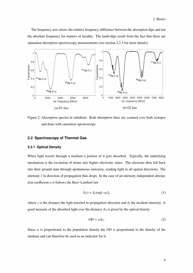
The frequency axis shows the relative frequency difference between the absorption dips and not
the absolute frequency for matters of lucidity. The lamb-dips result from the fact that these are
saturation absorption spectroscopy measurements (see section 2.2.3 for more details).
0 2000 4000 6000 8000
rel. frequency [MHz]
0
0.2
0.4
0.6
0.8
1
Tra
nsm
issio
n
87Rb F=2
85Rb F=3
85Rb F=2
87Rb F=1
(a) D1 line
0 1000 2000 3000 4000 5000 6000 7000 8000
rel. frequency [MHz]
0
0.2
0.4
0.6
0.8
1
Tra
nsm
issio
n
87Rb F=2
85Rb F=3
85Rb F=2
87Rb F=1
(b) D2 line
Figure 2: Absorption spectra in rubidium. Both absorption lines are scanned over both isotopes
and done with saturation spectroscopy.
2.2 Spectroscopy of Thermal Gas
2.2.1 Optical Density
When light travels through a medium a portion of it gets absorbed. Typically, the underlying
mechanism is the excitation of atoms into higher electronic states. The electrons then fall back
into their ground state through spontaneous emission, sending light in all spatial directions. The
intensity I in direction of propagation thus drops. In the case of an intensity independent absorp-
tion coefficient α it follows the Beer–Lambert law
I(z) = I0 exp[−αz], (1)
where z is the distance the light traveled in propagation direction and I0 the incident intensity. A
good measure of the absorbed light over the distance ∆z is given by the optical density
OD = α∆z. (2)
Since α is proportional to the population density the OD is proportional to the density of the
medium and can therefore be used as an indicator for it.
4
2 Basics
2.2.2 Broadening Mechanisms
In spectroscopy measurements the observed spectral lines are not strict monochromatic. There are
different broadening mechanisms that lead to distinct half widths. The most important ones in the
case of a thermal gas will be discussed in the following section.
The natural linewidth originates from the fact that the atomic states have a natural lifetime τ.
The transition of an atom can be viewed as a damped harmonic oscillator, where the damping
comes from the natural lifetime of the involved states. This results in a Lorentz-profile for the
observed spectral line [6]
L(ω) =Ak,i/2π
(ω − ω0)2 + (Ak,i/2)2 . (3)
with the normalization ∫ ∞
0L(ω)dω = 1 (4)
Here ω0 is the eigenfrequency of the system and Ak,i the Einstein coefficient of the transition from
state k to i. This results in a line width of ωL = 1/τk + 1/τi.
For the spectroscopy of thermal gas the movement of the atoms also plays an important role.
Because of the movement the observed frequency shifts from the eigenfrequency ω0 to ω = ω0 −
k · v, dependent of the velocity v of the atoms and the wave vector k of the emitted light. The
Maxwell-Boltzmann distribution leads to an overlap of the different shifts, resulting in a Gaussian
profile [6]
G(ω) = exp
−4 ln(2)(ω − ω0
ωD
)2 . (5)
This is called Doppler broadening with the Doppler width of ωD =ω0c
√2kBT ·4 ln(2)
m .
The pressure broadening is also an important broadening mechanism. It emerges when two
atoms collide or get close to each other. The interaction leads to a shift of the energy levels and a
reduction of the life time of the excited state. For an elastic collision the energies only get shifted
during the collision and the line shiftes by ∆ω = ω0−|EA(R)−EB(R)|
~ , where the energies of the atoms
A and B are dependent on the distance R between the atoms. For an inelastic collision the energy
of the collision partners gets (for a part or as whole) translated into inner energy or kinetic energy.
As a result of both processes, the line is broadened resembling a Lorentzian profile.
Another broadening mechanism is caused by the laser power and called power broadening. The
population density of the ground state of a two level atom depends on the pumprate P of the laser
and the relaxation probability R1,R2 of the involved states. For high values of P the population
difference is given by
∆N =∆N(P = 0)
1 + Swith S =
2PR1 + R2
. (6)
5
2 Basics
For R1 = 0 the saturation parameter S can be written as S (ω) =2σ12(ω)I(ω)~ωA12
, being dependent on
the intensity I of the laser. Since the absorption coefficient α =α0
1+S gets a frequency dependency
through the saturation parameter the line gets broadened with
∆ωS = ∆ω0√
1 + S (ω = ω0). (7)
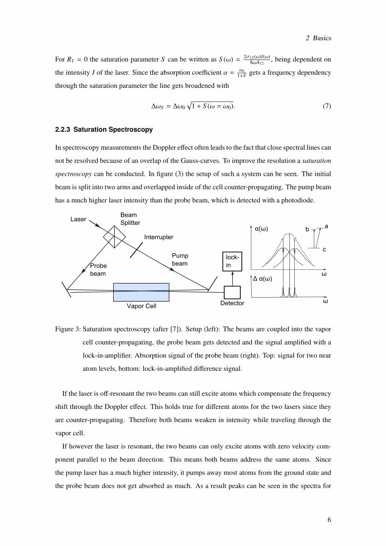
2.2.3 Saturation Spectroscopy
In spectroscopy measurements the Doppler effect often leads to the fact that close spectral lines can
not be resolved because of an overlap of the Gauss-curves. To improve the resolution a saturation
spectroscopy can be conducted. In figure (3) the setup of such a system can be seen. The initial
beam is split into two arms and overlapped inside of the cell counter-propagating. The pump beam
has a much higher laser intensity than the probe beam, which is detected with a photodiode.
Laser
Probe
beam
Pump
beam
Interrupter
Beam
Splitter
Detector
lock-
in
Vapor Cell
α ω
Δ α(ω)
ω
ω
ab
c
Figure 3: Saturation spectroscopy (after [7]). Setup (left): The beams are coupled into the vapor
cell counter-propagating, the probe beam gets detected and the signal amplified with a
lock-in-amplifier. Absorption signal of the probe beam (right). Top: signal for two near
atom levels, bottom: lock-in-amplified difference signal.
If the laser is off-resonant the two beams can still excite atoms which compensate the frequency
shift through the Doppler effect. This holds true for different atoms for the two lasers since they
are counter-propagating. Therefore both beams weaken in intensity while traveling through the
vapor cell.
If however the laser is resonant, the two beams can only excite atoms with zero velocity com-
ponent parallel to the beam direction. This means both beams address the same atoms. Since
the pump laser has a much higher intensity, it pumps away most atoms from the ground state and
the probe beam does not get absorbed as much. As a result peaks can be seen in the spectra for
6
2 Basics
on-resonant frequencies (see figure (3) right top). These are called lamb-dips. Right in the middle
of the resonance frequencies of two hyperfine states an additional lamb-dip appears, the so called
cross-over-resonance. It appears because at this frequency the two lasers excite the same moving
atom into the different exited states due to the Doppler shift.
The signal-to-noise ratio of the signal can be improved with the help of a lock-in amplifier. To
do this the pump laser is modulated with an interrupter so that the appearance of lamb-dips in the
probe signal gets modulated accordingly. The lock-in amplifier now amplifies the signal through
phase-sensitive detection. Additionally the Gaussian background of the spectrum can be removed
(see figure (3) right bottom) with a differential lock-in-amplifier, which amplifies the difference of
the signal with and without the pump beam.
2.3 Hollow Core Fibers
Hollow core fibers have, as the name indicates, a hollow core in contrast to solid core fiber or
conventional optical fibers. This core can be filled with gas or liquid which then overlaps very
well with light guided alongside the fiber core. In optical fibers the guiding mechanism is based
on total internal reflection of the light at the cladding with a lower refractive index than the core.
For hollow core fibers this is not possible since there is no cladding material with n < 1 available.
Here the guiding mechanisms are based on different effects, depending of the structure of the fiber.
In general there are three different fiber types: the capillaries, the bandgap hollow-core photonic
fibers (BG-HCPCF) and the kagome lattice fibers.
The core of the BG-HCPCF is surrounded by a honey-comb lattice which builds up a band-
gap. This band-gap results in frequency domains in which light can not travel through the fiber
and gets trapped in it. The BG-HCPCF usually have a very narrow transmission band width of
around 100 nm.
In this thesis the fibers used are the capillary and the kagome fiber. Therefore these two will be
discussed in more detail.
2.3.1 Capillary
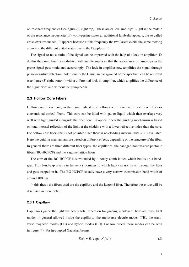
Capillaries guide the light via nearly total reflection for gracing incidence.There are three light
modes in general allowed inside the capillary: the transverse electric modes (TE), the trans-
verse magnetic modes (EH) and hybrid modes (EH). For low orders these modes can be seen
in figure (4). For in-coupled Gaussian beams
E(r) = E0 exp(−r2/ω2) (8)
7
2 Basics
only EH1m field modes can be excited [8]. They can be approximated with the Bessel-function J
E(r) = E0J0(umra
) (9)
for fibers of radius a. um is the m-th root of the zero order Bessel function J0. For the lowest loss
mode EH11, the highest coupling efficiency of 98.1% is reached for a beam waist to core ratio of
ω/a = 0.64 [8].
TE TM EH01 01 11
Figure 4: Schematics for possible light fields inside a hollow core fiber. Given are low order modes
of transverse electric (TE), transverse magnetic (TM) and hybrid (EH) field modes. For
Gaussian beams the EH11 is the lowest loss mode.
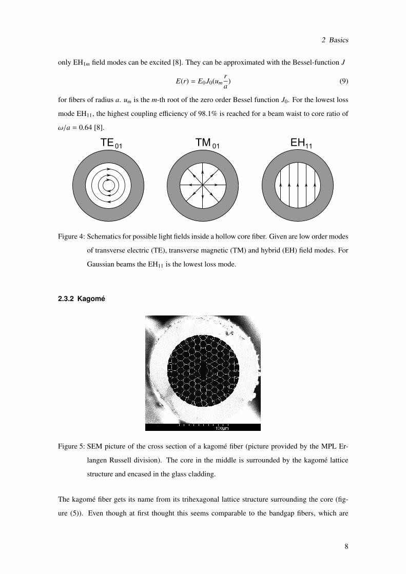
2.3.2 Kagome
Figure 5: SEM picture of the cross section of a kagome fiber (picture provided by the MPL Er-
langen Russell division). The core in the middle is surrounded by the kagome lattice
structure and encased in the glass cladding.
The kagome fiber gets its name from its trihexagonal lattice structure surrounding the core (fig-
ure (5)). Even though at first thought this seems comparable to the bandgap fibers, which are
8
2 Basics
surrounded by a honeycomb lattice structure, the guiding mechanism of the kagome is based on
a different effect. The kagome fiber has no bandgap that confines the light, rather anti-resonance
properties in the first ring of holes provide the guidiance of the light [9]. In comparison to bandgap
fibers this leads to broader transmission bands but also to higher losses.
2.4 Diffusion in Thin Tubes
The propagation of light in hollow core fibers has been discussed in the previous section. In this
section the propagation of atoms inside the core is discussed.
The diffusion properties of gas into a thin tube are determined by the Knudsen number Kn = λ2r ,
with λ being the mean free path of the gas molecules and r the radius of the tube. If Kn 1 it
means that the gas molecules mainly collide with each other and that collision with the tube wall
can be neglected and the dynamics can be described by the Navier-Stokes-equations. If Kn 1
(which will be the case in this thesis) the molecules have a long mean free path and collide mainly
with the tube wall. The dynamics in this case can be described with a one-dimensional diffusion
equation [10]∂n∂t
= D∂2n∂x2 . (10)
Here n(x, t) is the atomic density inside the thin tube for the time t at position x and D is the
diffusion constant, which for thin tubes is given by [10]
D =43
r2
τ + (2r/v). (11)
Here v =√
8kBT/(πm) is the mean velocity of the gas atoms with their mass m. The adsorption
time τ is dependent on the adsorption energy Ea, the temperature of the tube wall Tw and the
characteristic absorption time τ0:
τ = τ0 exp[
Ea
kBTW
]. (12)
τ can be interpreted as the mean time an adsorbed atom stays on the wall and is therefore inverse
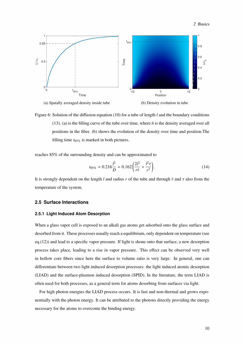
proportional to the adsorbtion rate ν = 1/τ. The solution of the diffusion equation (10) can be seen
in figure (6) for a thin tube of lenght l and with the following boundary conditions:
n(t = 0, x) = 0 for − l/2 < x < l/2
n(t, x = ±l/2) = n0 for all t. (13)
The tube is empty at time t = 0 and gets filled via diffusion from the surrounding atomic density
n0. In [3] the filling time of a thin tube is defined as the time when the density inside the tube
9
2 Basics
0 t85%
Time
0
0.5
0.85
1n/n0
(a) Spatally averaged density inside tube
-l/2 0 l/2
Position
0
t85%
Tim
e
0
0.2
0.4
0.6
0.8
1
n/n
0
(b) Density evolution in tube
Figure 6: Solution of the diffusion equation (10) for a tube of length l and the boundary conditions
(13). (a) is the filling curve of the tube over time, where n is the density averaged over all
positions in the fiber. (b) shows the evolution of the density over time and position.The
filling time t85% is marked in both pictures.
reaches 85% of the surrounding density and can be approximated to
t85% ≈ 0.216l2
D= 0.162
(2l2
rv+
l2τr2
). (14)
It is strongly dependent on the length l and radius r of the tube and through v and τ also from the
temperature of the system.
2.5 Surface Interactions
2.5.1 Light Induced Atom Desorption
When a glass vapor cell is exposed to an alkali gas atoms get adsorbed onto the glass surface and
desorbed from it. These processes usually reach a equilibrium, only dependent on temperature (see
eq.(12)) and lead to a specific vapor pressure. If light is shone onto that surface, a new desorption
process takes place, leading to a rise in vapor pressure. This effect can be observed very well
in hollow core fibers since here the surface to volume ratio is very large. In general, one can
differentiate between two light induced desorption processes: the light induced atomic desorption
(LIAD) and the surface-plasmon induced desorption (SPID). In the literature, the term LIAD is
often used for both processes, as a general term for atoms desorbing from surfaces via light.
For high photon energies the LIAD process occurs. It is fast and non-thermal and grows expo-
nentially with the photon energy. It can be attributed to the photons directly providing the energy
necessary for the atoms to overcome the binding energy.
10
2 Basics
For lower photon energies the dominating effect is the SPID. For rubidium this photon energy
is typically around 1.5 eV [11] which correspondes to a wavelength of around 827 nm. In this
case the desorption process is caused by a surface-plasmon getting excited (heating), which then
acts as a catalyst for non-thermal desorption of an atom. This leads to an effective evaporation of
nanoclusters (i.e. ”small droplets” of the alkalis).
A third effect should also be mentioned: the effect of light induced diffusion inside the glass
bulk. Atoms do not only get adsorbed to the surface but diffuse into the bulk. If now atoms
from the surface are desorbed through LIAD or SPID, atoms inside the bulk start to diffuse to the
surface, where they can also get desorbed via the light. The atoms in the bulk can act therefore as
a slowly depleting reservoir during the LIAD process.
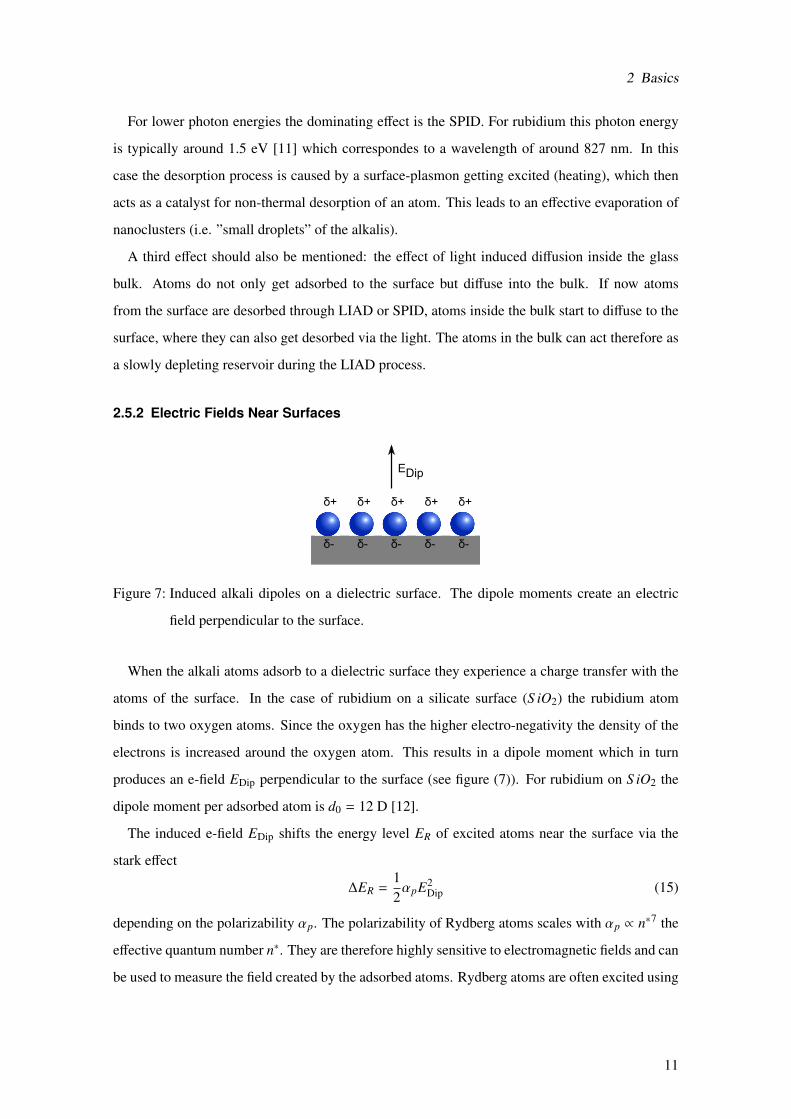
2.5.2 Electric Fields Near Surfaces
δ-
δ+
δ-δ-δ-δ-
δ+δ+δ+δ+
EDip
Figure 7: Induced alkali dipoles on a dielectric surface. The dipole moments create an electric
field perpendicular to the surface.
When the alkali atoms adsorb to a dielectric surface they experience a charge transfer with the
atoms of the surface. In the case of rubidium on a silicate surface (S iO2) the rubidium atom
binds to two oxygen atoms. Since the oxygen has the higher electro-negativity the density of the
electrons is increased around the oxygen atom. This results in a dipole moment which in turn
produces an e-field EDip perpendicular to the surface (see figure (7)). For rubidium on S iO2 the
dipole moment per adsorbed atom is d0 = 12 D [12].
The induced e-field EDip shifts the energy level ER of excited atoms near the surface via the
stark effect
∆ER =12αpE2
Dip (15)
depending on the polarizability αp. The polarizability of Rydberg atoms scales with αp ∝ n∗7 the
effective quantum number n∗. They are therefore highly sensitive to electromagnetic fields and can
be used to measure the field created by the adsorbed atoms. Rydberg atoms are often excited using
11
2 Basics
a two- or three-photon transitions. This can lead to new effects in comparison to a one-photon
transition.
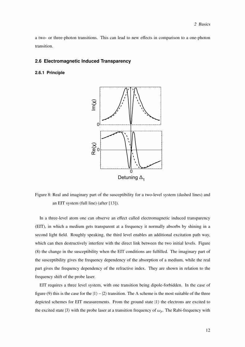
2.6 Electromagnetic Induced Transparency
2.6.1 Principle
Detuning 1
0
Re(
)Im
()
0
0
Figure 8: Real and imaginary part of the susceptibility for a two-level system (dashed lines) and
an EIT system (full line) (after [13]).
In a three-level atom one can observe an effect called electromagnetic induced transparency
(EIT), in which a medium gets transparent at a frequency it normally absorbs by shining in a
second light field. Roughly speaking, the third level enables an additional excitation path way,
which can then destructively interfere with the direct link between the two initial levels. Figure
(8) the change in the susceptibility when the EIT conditions are fulfilled. The imaginary part of
the susceptibility gives the frequency dependency of the absorption of a medium, while the real
part gives the frequency dependency of the refractive index. They are shown in relation to the
frequency shift of the probe laser.
EIT requires a three level system, with one transition being dipole-forbidden. In the case of
figure (9) this is the case for the |1〉 − |2〉 transition. The Λ scheme is the most suitable of the three
depicted schemes for EIT measurements. From the ground state |1〉 the electrons are excited to
the excited state |3〉 with the probe laser at a transition frequency of ωp. The Rabi-frequency with
12
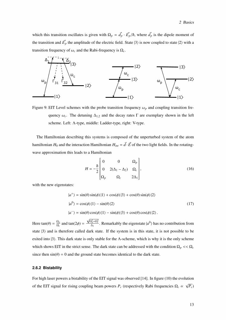
2 Basics
which this transition oscillates is given with Ωp = ~dp · ~Ep/~, where ~dp is the dipole moment of
the transition and ~Ep the amplitude of the electric field. State |3〉 is now coupled to state |2〉 with a
transition frequency of ωc and the Rabi-frequency is Ωc.
|1 |1 |1
|2
|2
|2
|3
|3
|3
p
c
Δ2
Δ1
Γ31Γ32
ωp
ωc
ωc
ωp
Figure 9: EIT Level schemes with the probe transition frequency ωp and coupling transition fre-
quency ωc. The detuning ∆1,2 and the decay rates Γ are exemplary shown in the left
scheme. Left: Λ-type, middle: Ladder-type, right: V-type.
The Hamiltonian describing this systems is composed of the unperturbed system of the atom
hamiltonian H0 and the interaction Hamiltonian Hint = ~d · ~E of the two light fields. In the rotating-
wave approximation this leads to a Hamiltonian
H = −~
2
0 0 Ωp
0 2(∆1 − ∆2) Ωc
Ωp Ωc 2∆1
, (16)
with the new eigenstates:
|a+〉 = sin(θ) sin(φ) |1〉 + cos(φ) |3〉 + cos(θ) sin(φ) |2〉
|a0〉 = cos(φ) |1〉 − sin(θ) |2〉 (17)
|a−〉 = sin(θ) cos(φ) |1〉 − sin(φ) |3〉 + cos(θ) cos(φ) |2〉 .
Here tan(θ) =ΩpΩc
and tan(2φ) =
√Ω2
p+Ω2c
∆1. Remarkably the eigenstate |a0〉 has no contribution from
state |3〉 and is therefore called dark state. If the system is in this state, it is not possible to be
exited into |3〉. This dark state is only stable for the Λ-scheme, which is why it is the only scheme
which shows EIT in the strict sense. The dark state can be addressed with the condition Ωp << Ωc
since then sin(θ) = 0 and the ground state becomes identical to the dark state.
2.6.2 Bistability
For high laser powers a bistability of the EIT signal was observed [14]. In figure (10) the evolution
of the EIT signal for rising coupling beam powers Pc (respectively Rabi frequencies Ωc ∝√
Pc)
13
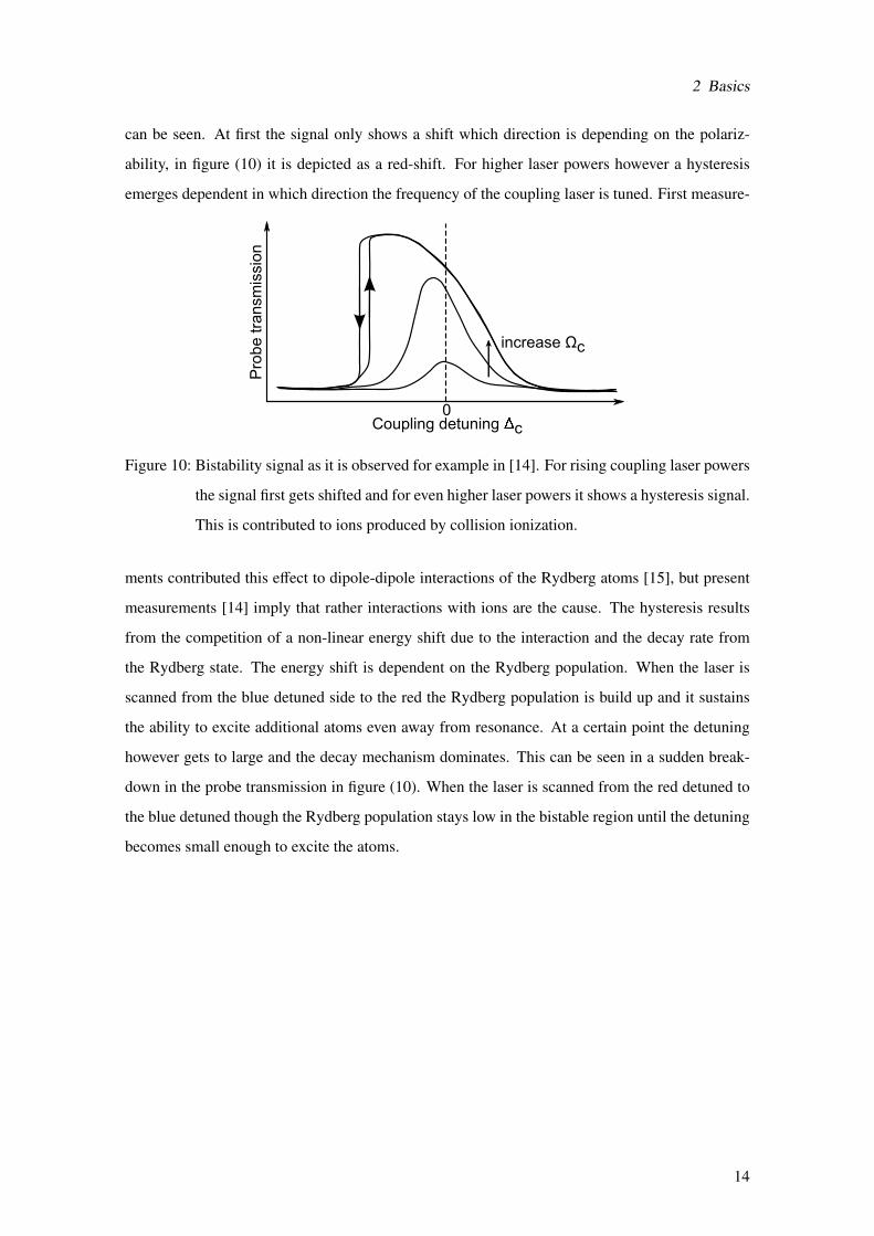
2 Basics
can be seen. At first the signal only shows a shift which direction is depending on the polariz-
ability, in figure (10) it is depicted as a red-shift. For higher laser powers however a hysteresis
emerges dependent in which direction the frequency of the coupling laser is tuned. First measure-
Coupling detuning c
Pro
be
tra
nsm
issio
n
0
increase Ωc
Figure 10: Bistability signal as it is observed for example in [14]. For rising coupling laser powers
the signal first gets shifted and for even higher laser powers it shows a hysteresis signal.
This is contributed to ions produced by collision ionization.
ments contributed this effect to dipole-dipole interactions of the Rydberg atoms [15], but present
measurements [14] imply that rather interactions with ions are the cause. The hysteresis results
from the competition of a non-linear energy shift due to the interaction and the decay rate from
the Rydberg state. The energy shift is dependent on the Rydberg population. When the laser is
scanned from the blue detuned side to the red the Rydberg population is build up and it sustains
the ability to excite additional atoms even away from resonance. At a certain point the detuning
however gets to large and the decay mechanism dominates. This can be seen in a sudden break-
down in the probe transmission in figure (10). When the laser is scanned from the red detuned to
the blue detuned though the Rydberg population stays low in the bistable region until the detuning
becomes small enough to excite the atoms.
14
3 Fiber Series: Spectroscopy Below the Doppler Limit
3 Fiber Series: Spectroscopy Below the Doppler Limit
3.1 Setup
3.1.1 Cell
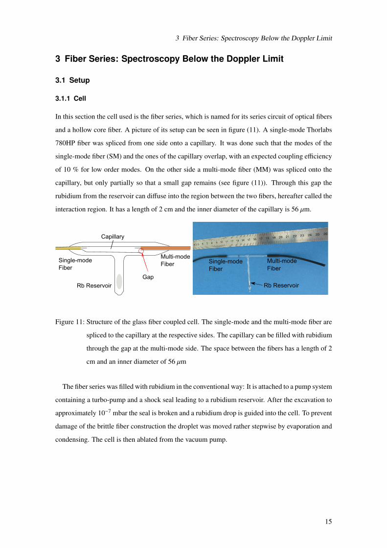
In this section the cell used is the fiber series, which is named for its series circuit of optical fibers
and a hollow core fiber. A picture of its setup can be seen in figure (11). A single-mode Thorlabs
780HP fiber was spliced from one side onto a capillary. It was done such that the modes of the
single-mode fiber (SM) and the ones of the capillary overlap, with an expected coupling efficiency
of 10 % for low order modes. On the other side a multi-mode fiber (MM) was spliced onto the
capillary, but only partially so that a small gap remains (see figure (11)). Through this gap the
rubidium from the reservoir can diffuse into the region between the two fibers, hereafter called the
interaction region. It has a length of 2 cm and the inner diameter of the capillary is 56 µm.
Single-mode
Fiber
Multi-mode
Fiber
Rb Reservoir
Gap
Capillary
Rb Reservoir
Single-mode
Fiber
Multi-mode
Fiber
Figure 11: Structure of the glass fiber coupled cell. The single-mode and the multi-mode fiber are
spliced to the capillary at the respective sides. The capillary can be filled with rubidium
through the gap at the multi-mode side. The space between the fibers has a length of 2
cm and an inner diameter of 56 µm
The fiber series was filled with rubidium in the conventional way: It is attached to a pump system
containing a turbo-pump and a shock seal leading to a rubidium reservoir. After the excavation to
approximately 10−7 mbar the seal is broken and a rubidium drop is guided into the cell. To prevent
damage of the brittle fiber construction the droplet was moved rather stepwise by evaporation and
condensing. The cell is then ablated from the vacuum pump.
15
3 Fiber Series: Spectroscopy Below the Doppler Limit
3.1.2 Oven
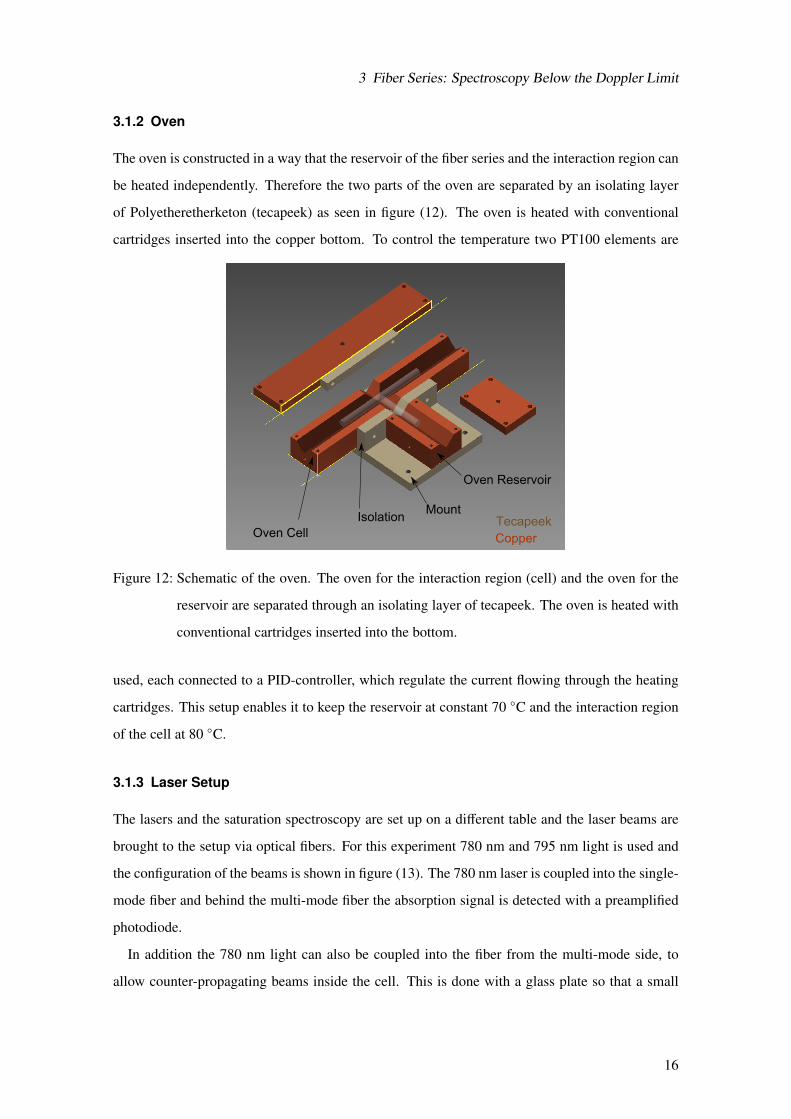
The oven is constructed in a way that the reservoir of the fiber series and the interaction region can
be heated independently. Therefore the two parts of the oven are separated by an isolating layer
of Polyetheretherketon (tecapeek) as seen in figure (12). The oven is heated with conventional
cartridges inserted into the copper bottom. To control the temperature two PT100 elements are
CopperOven Cell
Oven Reservoir
MountIsolation Tecapeek
Figure 12: Schematic of the oven. The oven for the interaction region (cell) and the oven for the
reservoir are separated through an isolating layer of tecapeek. The oven is heated with
conventional cartridges inserted into the bottom.
used, each connected to a PID-controller, which regulate the current flowing through the heating
cartridges. This setup enables it to keep the reservoir at constant 70 C and the interaction region
of the cell at 80 C.
3.1.3 Laser Setup
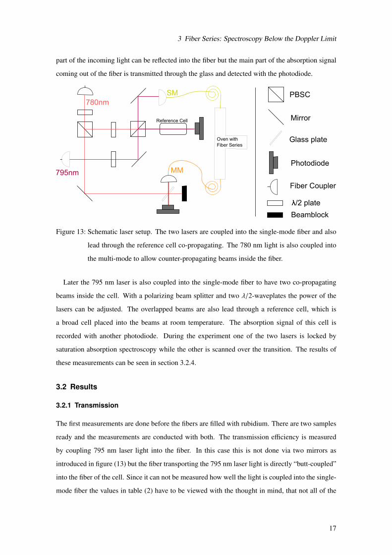
The lasers and the saturation spectroscopy are set up on a different table and the laser beams are
brought to the setup via optical fibers. For this experiment 780 nm and 795 nm light is used and
the configuration of the beams is shown in figure (13). The 780 nm laser is coupled into the single-
mode fiber and behind the multi-mode fiber the absorption signal is detected with a preamplified
photodiode.
In addition the 780 nm light can also be coupled into the fiber from the multi-mode side, to
allow counter-propagating beams inside the cell. This is done with a glass plate so that a small
16
3 Fiber Series: Spectroscopy Below the Doppler Limit
part of the incoming light can be reflected into the fiber but the main part of the absorption signal
coming out of the fiber is transmitted through the glass and detected with the photodiode.
795nm
780nm
MM
SM
Oven with
Fiber Series
PBSC
Mirror
Photodiode
/2 plate
Beamblock
Glass plate
Fiber Coupler
Reference Cell
Figure 13: Schematic laser setup. The two lasers are coupled into the single-mode fiber and also
lead through the reference cell co-propagating. The 780 nm light is also coupled into
the multi-mode to allow counter-propagating beams inside the fiber.
Later the 795 nm laser is also coupled into the single-mode fiber to have two co-propagating
beams inside the cell. With a polarizing beam splitter and two λ/2-waveplates the power of the
lasers can be adjusted. The overlapped beams are also lead through a reference cell, which is
a broad cell placed into the beams at room temperature. The absorption signal of this cell is
recorded with another photodiode. During the experiment one of the two lasers is locked by
saturation absorption spectroscopy while the other is scanned over the transition. The results of
these measurements can be seen in section 3.2.4.
3.2 Results
3.2.1 Transmission
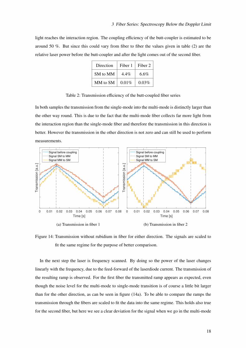
The first measurements are done before the fibers are filled with rubidium. There are two samples
ready and the measurements are conducted with both. The transmission efficiency is measured
by coupling 795 nm laser light into the fiber. In this case this is not done via two mirrors as
introduced in figure (13) but the fiber transporting the 795 nm laser light is directly “butt-coupled”
into the fiber of the cell. Since it can not be measured how well the light is coupled into the single-
mode fiber the values in table (2) have to be viewed with the thought in mind, that not all of the
17
3 Fiber Series: Spectroscopy Below the Doppler Limit
light reaches the interaction region. The coupling efficiency of the butt-coupler is estimated to be
around 50 %. But since this could vary from fiber to fiber the values given in table (2) are the
relative laser power before the butt-coupler and after the light comes out of the second fiber.
Direction Fiber 1 Fiber 2
SM to MM 4.4% 6.6%
MM to SM 0.01% 0.03%
Table 2: Transmission efficiency of the butt-coupled fiber series
In both samples the transmission from the single-mode into the multi-mode is distinctly larger than
the other way round. This is due to the fact that the multi-mode fiber collects far more light from
the interaction region than the single-mode fiber and therefore the transmission in this direction is
better. However the transmission in the other direction is not zero and can still be used to perform
measurements.
0 0.01 0.02 0.03 0.04 0.05 0.06 0.07 0.08
Time [s]
Tra
nsm
issio
n [
a.u
.]
Signal before coupling
Signal SM to MM
Signal MM to SM
(a) Transmission in fiber 1
0 0.01 0.02 0.03 0.04 0.05 0.06 0.07 0.08
Time [s]
Tra
nsm
issio
n [
a.u
.]
Signal before coupling
Signal SM to MM
Signal MM to SM
(b) Transmission in fiber 2
Figure 14: Transmission without rubidium in fiber for either direction. The signals are scaled to
fit the same regime for the purpose of better comparison.
In the next step the laser is frequency scanned. By doing so the power of the laser changes
linearly with the frequency, due to the feed-forward of the laserdiode current. The transmission of
the resulting ramp is observed. For the first fiber the transmitted ramp appears as expected, even
though the noise level for the multi-mode to single-mode transition is of course a little bit larger
than for the other direction, as can be seen in figure (14a). To be able to compare the ramps the
transmission through the fibers are scaled to fit the data into the same regime. This holds also true
for the second fiber, but here we see a clear deviation for the signal when we go in the multi-mode
18
3 Fiber Series: Spectroscopy Below the Doppler Limit
to single-mode direction, and with small nudges on the fiber the signal fluctuates strongly.
Fiber 1 is the first one to be filled with rubidium. Unfortunately the fibers broke, most likely
during the filling or the transport of the fiber. In both, the single-mode and the multi-mode fiber,
one could see a rupture under the microscope and the transmission efficiency in the direction
single-mode to multi-mode dropped to 0.05%. Therefore all the following measurements are done
with the second sample.
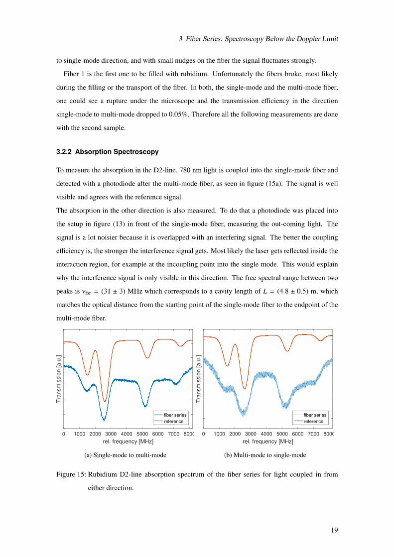
3.2.2 Absorption Spectroscopy
To measure the absorption in the D2-line, 780 nm light is coupled into the single-mode fiber and
detected with a photodiode after the multi-mode fiber, as seen in figure (15a). The signal is well
visible and agrees with the reference signal.
The absorption in the other direction is also measured. To do that a photodiode was placed into
the setup in figure (13) in front of the single-mode fiber, measuring the out-coming light. The
signal is a lot noisier because it is overlapped with an interfering signal. The better the coupling
efficiency is, the stronger the interference signal gets. Most likely the laser gets reflected inside the
interaction region, for example at the incoupling point into the single mode. This would explain
why the interference signal is only visible in this direction. The free spectral range between two
peaks is νfsr = (31 ± 3) MHz which corresponds to a cavity length of L = (4.8 ± 0.5) m, which
matches the optical distance from the starting point of the single-mode fiber to the endpoint of the
multi-mode fiber.
0 1000 2000 3000 4000 5000 6000 7000 8000
rel. frequency [MHz]
Tra
nsm
issio
n [a.u
.]
fiber series
reference
(a) Single-mode to multi-mode
0 1000 2000 3000 4000 5000 6000 7000 8000
rel. frequency [MHz]
Tra
nsm
issio
n [a.u
.]
fiber series
reference
(b) Multi-mode to single-mode
Figure 15: Rubidium D2-line absorption spectrum of the fiber series for light coupled in from
either direction.
19
3 Fiber Series: Spectroscopy Below the Doppler Limit
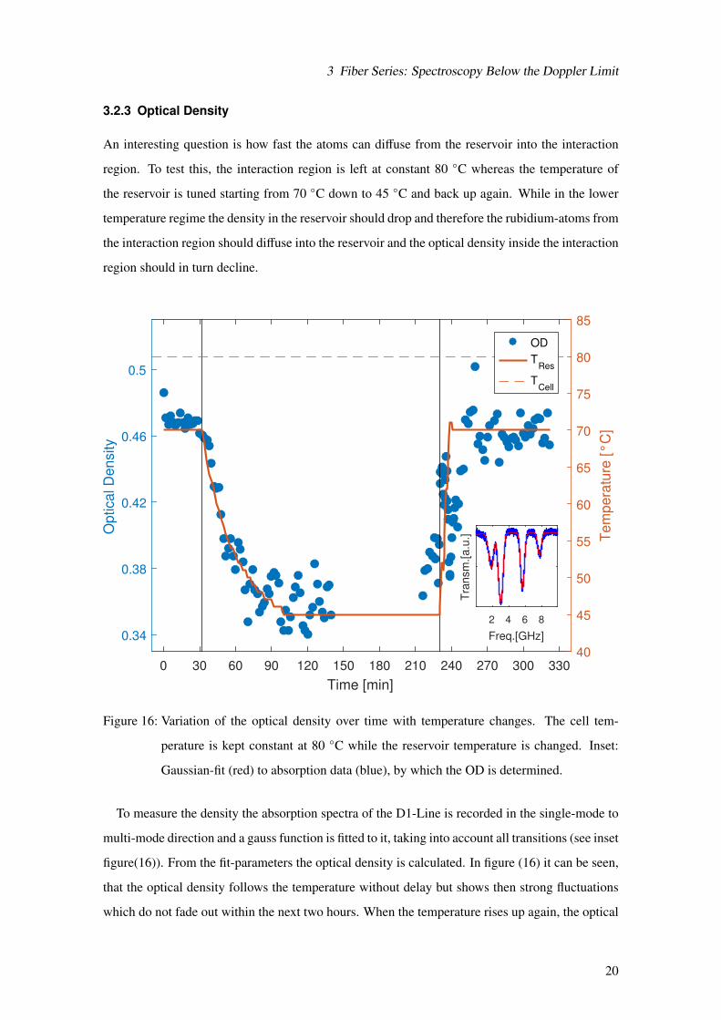
3.2.3 Optical Density
An interesting question is how fast the atoms can diffuse from the reservoir into the interaction
region. To test this, the interaction region is left at constant 80 C whereas the temperature of
the reservoir is tuned starting from 70 C down to 45 C and back up again. While in the lower
temperature regime the density in the reservoir should drop and therefore the rubidium-atoms from
the interaction region should diffuse into the reservoir and the optical density inside the interaction
region should in turn decline.
0 30 60 90 120 150 180 210 240 270 300 330
Time [min]
0.34
0.38
0.42
0.46
0.5
Optical D
ensity
40
45
50
55
60
65
70
75
80
85
Tem
pera
ture
[°
C]
OD
TRes
TCell
2 4 6 8
Freq.[GHz]
Tra
nsm
.[a
.u.]
Figure 16: Variation of the optical density over time with temperature changes. The cell tem-
perature is kept constant at 80 C while the reservoir temperature is changed. Inset:
Gaussian-fit (red) to absorption data (blue), by which the OD is determined.
To measure the density the absorption spectra of the D1-Line is recorded in the single-mode to
multi-mode direction and a gauss function is fitted to it, taking into account all transitions (see inset
figure(16)). From the fit-parameters the optical density is calculated. In figure (16) it can be seen,
that the optical density follows the temperature without delay but shows then strong fluctuations
which do not fade out within the next two hours. When the temperature rises up again, the optical
20
3 Fiber Series: Spectroscopy Below the Doppler Limit
density follows again nearly instantaneous and reaches a density a bit smaller and with stronger
fluctuations than before. Again, it will take several hours until the system equilibrates.
3.2.4 Subdoppler Spectroscopy
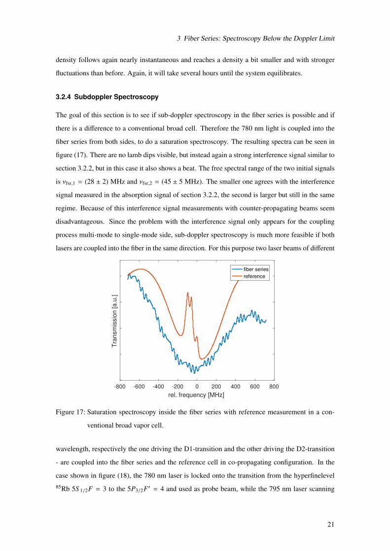
The goal of this section is to see if sub-doppler spectroscopy in the fiber series is possible and if
there is a difference to a conventional broad cell. Therefore the 780 nm light is coupled into the
fiber series from both sides, to do a saturation spectroscopy. The resulting spectra can be seen in
figure (17). There are no lamb dips visible, but instead again a strong interference signal similar to
section 3.2.2, but in this case it also shows a beat. The free spectral range of the two initial signals
is νfsr,1 = (28 ± 2) MHz and νfsr,2 = (45 ± 5 MHz). The smaller one agrees with the interference
signal measured in the absorption signal of section 3.2.2, the second is larger but still in the same
regime. Because of this interference signal measurements with counter-propagating beams seem
disadvantageous. Since the problem with the interference signal only appears for the coupling
process multi-mode to single-mode side, sub-doppler spectroscopy is much more feasible if both
lasers are coupled into the fiber in the same direction. For this purpose two laser beams of different
-800 -600 -400 -200 0 200 400 600 800
rel. frequency [MHz]
Tra
nsm
issio
n [
a.u
.]
fiber series
reference
Figure 17: Saturation spectroscopy inside the fiber series with reference measurement in a con-
ventional broad vapor cell.
wavelength, respectively the one driving the D1-transition and the other driving the D2-transition
- are coupled into the fiber series and the reference cell in co-propagating configuration. In the
case shown in figure (18), the 780 nm laser is locked onto the transition from the hyperfinelevel85Rb 5S 1/2F = 3 to the 5P3/2F′ = 4 and used as probe beam, while the 795 nm laser scanning
21
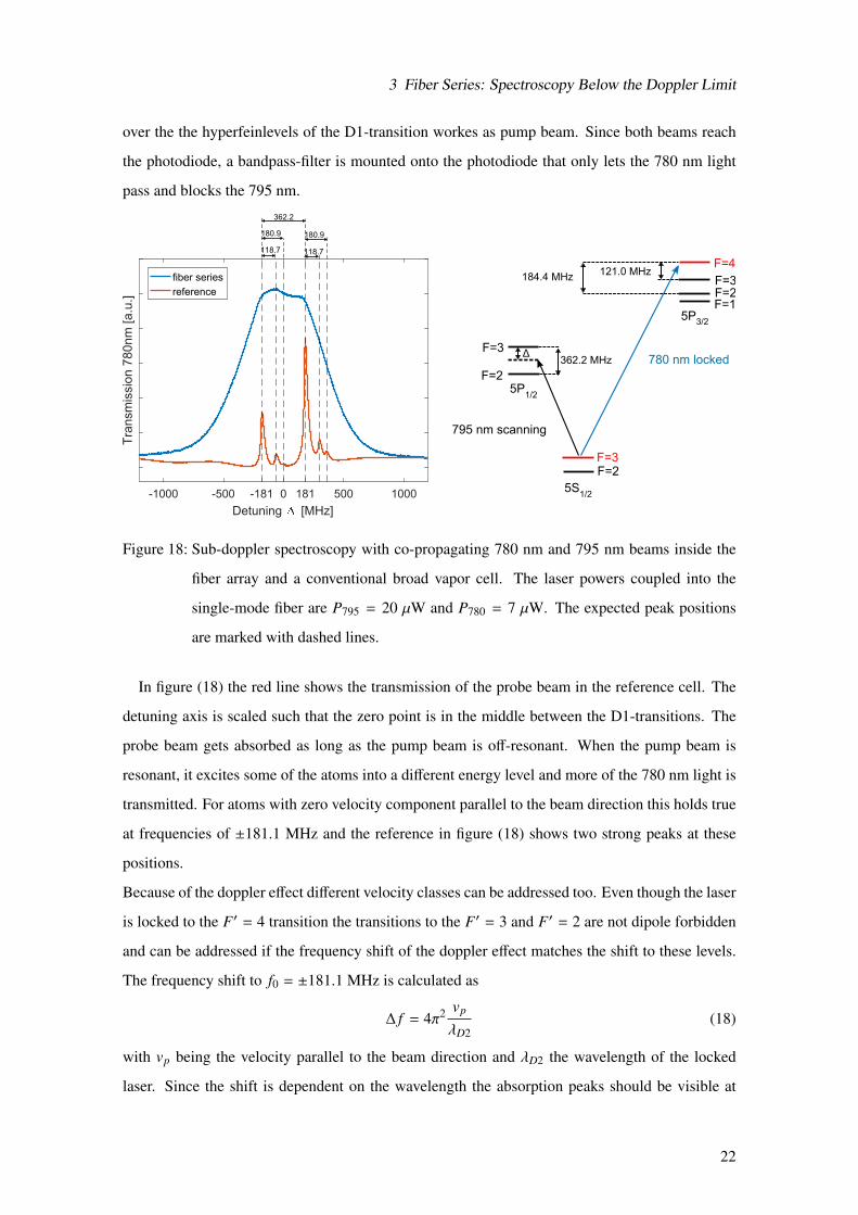
3 Fiber Series: Spectroscopy Below the Doppler Limit
over the the hyperfeinlevels of the D1-transition workes as pump beam. Since both beams reach
the photodiode, a bandpass-filter is mounted onto the photodiode that only lets the 780 nm light
pass and blocks the 795 nm.
-1000 -500 -181 0 181 500 1000
Detuning [MHz]
Tra
nsm
issio
n 7
80nm
[a.u
.]
fiber series
reference
118.7
180.9
118.7
180.9
362.2
F=2
F=2
F=3
F=2
F=3
F=3
F=4
F=1
5S1/2
5P1/2
5P3/2
780 nm locked
795 nm scanning
362.2 MHz
121.0 MHz184.4 MHz
Δ
Figure 18: Sub-doppler spectroscopy with co-propagating 780 nm and 795 nm beams inside the
fiber array and a conventional broad vapor cell. The laser powers coupled into the
single-mode fiber are P795 = 20 µW and P780 = 7 µW. The expected peak positions
are marked with dashed lines.
In figure (18) the red line shows the transmission of the probe beam in the reference cell. The
detuning axis is scaled such that the zero point is in the middle between the D1-transitions. The
probe beam gets absorbed as long as the pump beam is off-resonant. When the pump beam is
resonant, it excites some of the atoms into a different energy level and more of the 780 nm light is
transmitted. For atoms with zero velocity component parallel to the beam direction this holds true
at frequencies of ±181.1 MHz and the reference in figure (18) shows two strong peaks at these
positions.
Because of the doppler effect different velocity classes can be addressed too. Even though the laser
is locked to the F′ = 4 transition the transitions to the F′ = 3 and F′ = 2 are not dipole forbidden
and can be addressed if the frequency shift of the doppler effect matches the shift to these levels.
The frequency shift to f0 = ±181.1 MHz is calculated as
∆ f = 4π2 vp
λD2(18)
with vp being the velocity parallel to the beam direction and λD2 the wavelength of the locked
laser. Since the shift is dependent on the wavelength the absorption peaks should be visible at
22
3 Fiber Series: Spectroscopy Below the Doppler Limit
frequency shifts of
∆ fD1 = ∆ fλD2
λD1(19)
which correspond to ∆ fD1 = 118.7 MHz for the F′ = 3 transition and ∆ fD1 = 180.9 MHz for
the F′ = 2 transition. In figure (18) these positions are marked with dashed lines and they fit the
position of the peaks in the reference very well.
In comparison to the reference the signal of the fiber series is broadened. While the dominant
peaks of the reference have a full width half maximum of FWHMRef = 35 MHz the signal in the
fiber series is at FWHMSig = 598 MHz. This broadening is only slightly due to power broadening,
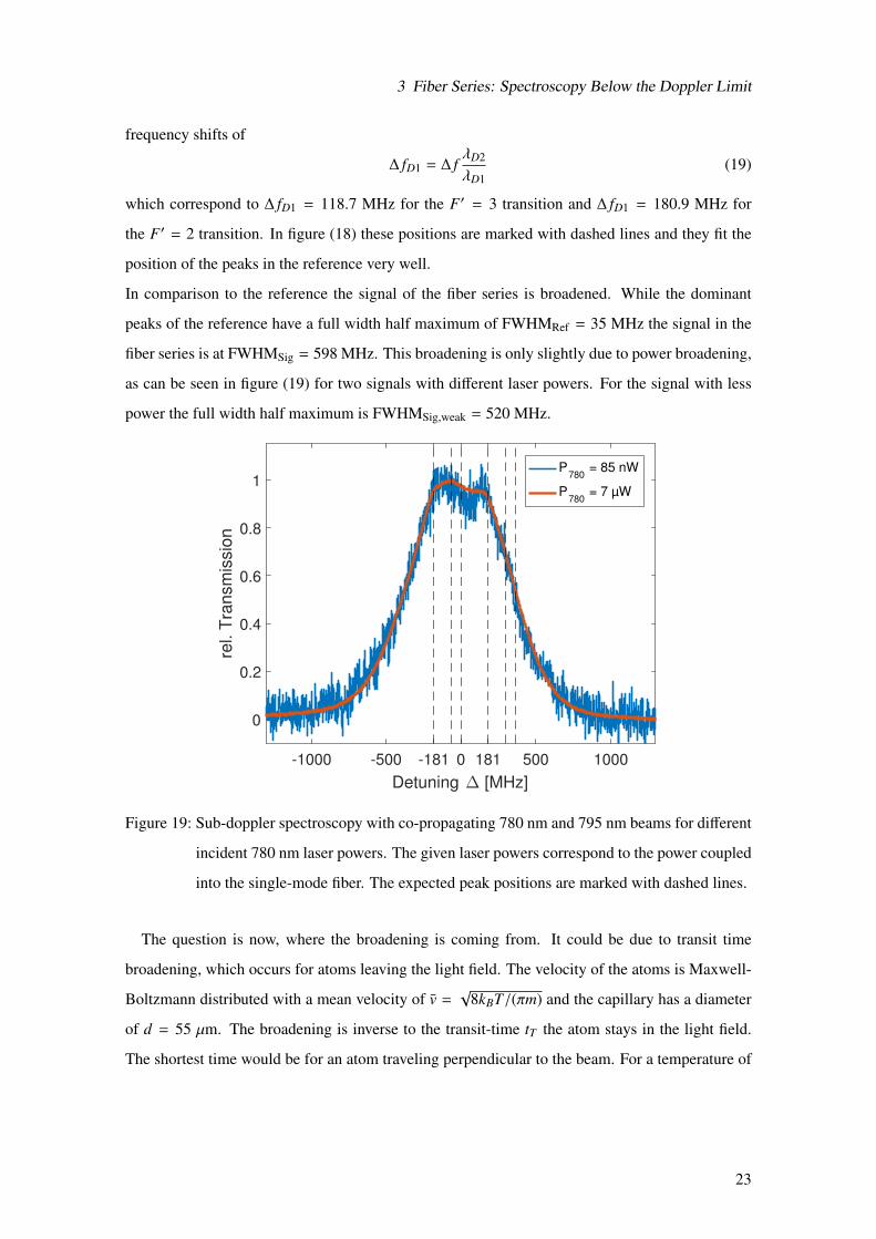
as can be seen in figure (19) for two signals with different laser powers. For the signal with less
power the full width half maximum is FWHMSig,weak = 520 MHz.
-1000 -500 -181 0 181 500 1000
Detuning ∆ [MHz]
0
0.2
0.4
0.6
0.8
1
rel. T
ran
sm
issio
n
P780
= 85 nW
P780
= 7 µW
Figure 19: Sub-doppler spectroscopy with co-propagating 780 nm and 795 nm beams for different
incident 780 nm laser powers. The given laser powers correspond to the power coupled
into the single-mode fiber. The expected peak positions are marked with dashed lines.
The question is now, where the broadening is coming from. It could be due to transit time
broadening, which occurs for atoms leaving the light field. The velocity of the atoms is Maxwell-
Boltzmann distributed with a mean velocity of v =√
8kBT/(πm) and the capillary has a diameter
of d = 55 µm. The broadening is inverse to the transit-time tT the atom stays in the light field.
The shortest time would be for an atom traveling perpendicular to the beam. For a temperature of
23
3 Fiber Series: Spectroscopy Below the Doppler Limit
80 C the transit-time broadening in this system should be
∆ FWHMtrans =1tT
=vd≈ 2π · 0.86 MHz, (20)
which is very small and does not explain a broadening of a few 100 MHz.
Another reason could be pressure broadening through contamination with other gases. If the
fiber series has a small leak air could diffuse into it. Air consists to 78% of N2. The power
broadening of the D2 line due to N2 is given in [16] as 18.3± 0.2 MHz/Torr. The weak signal was
broadened by 485 MHz, for this to be caused by pressure broadening with N2 the pressure inside
the fiber series has to be at 35.2 ± 0.4 mbar. This is pretty high but could be true if the fiber really
has a leak somewhere.
24
4 Hollow Core Fibers Encapsulated in All-Glass Vapor Cell: EIT Spectroscopy
4 Hollow Core Fibers Encapsulated in All-Glass Vapor Cell: EIT
Spectroscopy
4.1 Setup
4.1.1 Cell
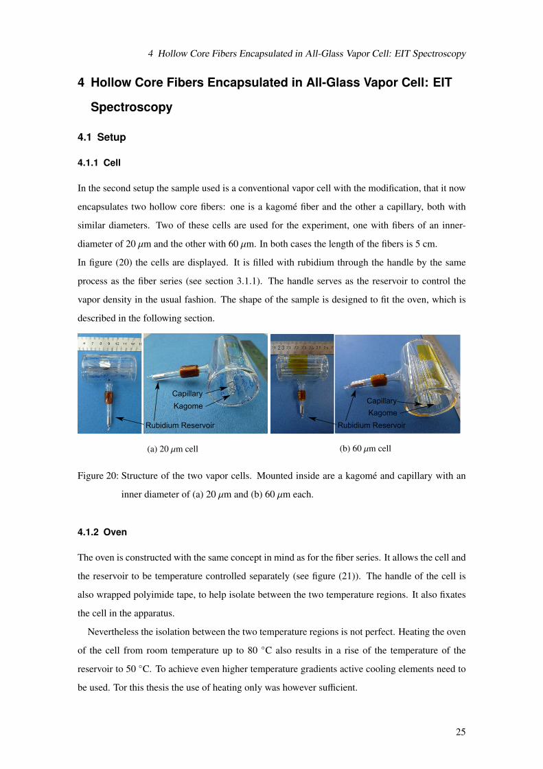
In the second setup the sample used is a conventional vapor cell with the modification, that it now
encapsulates two hollow core fibers: one is a kagome fiber and the other a capillary, both with
similar diameters. Two of these cells are used for the experiment, one with fibers of an inner-
diameter of 20 µm and the other with 60 µm. In both cases the length of the fibers is 5 cm.
In figure (20) the cells are displayed. It is filled with rubidium through the handle by the same
process as the fiber series (see section 3.1.1). The handle serves as the reservoir to control the
vapor density in the usual fashion. The shape of the sample is designed to fit the oven, which is
described in the following section.
Rubidium Reservoir
Kagome
Capillary
(a) 20 µm cell
Rubidium Reservoir
Kagome
Capillary
(b) 60 µm cell
Figure 20: Structure of the two vapor cells. Mounted inside are a kagome and capillary with an
inner diameter of (a) 20 µm and (b) 60 µm each.
4.1.2 Oven
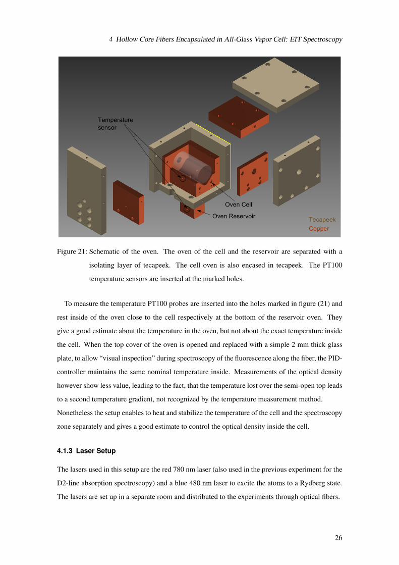
The oven is constructed with the same concept in mind as for the fiber series. It allows the cell and
the reservoir to be temperature controlled separately (see figure (21)). The handle of the cell is
also wrapped polyimide tape, to help isolate between the two temperature regions. It also fixates
the cell in the apparatus.
Nevertheless the isolation between the two temperature regions is not perfect. Heating the oven
of the cell from room temperature up to 80 C also results in a rise of the temperature of the
reservoir to 50 C. To achieve even higher temperature gradients active cooling elements need to
be used. Tor this thesis the use of heating only was however sufficient.
25
4 Hollow Core Fibers Encapsulated in All-Glass Vapor Cell: EIT Spectroscopy
Tecapeek
Copper
Oven Reservoir
Oven Cell
Temperature
sensor
Figure 21: Schematic of the oven. The oven of the cell and the reservoir are separated with a
isolating layer of tecapeek. The cell oven is also encased in tecapeek. The PT100
temperature sensors are inserted at the marked holes.
To measure the temperature PT100 probes are inserted into the holes marked in figure (21) and
rest inside of the oven close to the cell respectively at the bottom of the reservoir oven. They
give a good estimate about the temperature in the oven, but not about the exact temperature inside
the cell. When the top cover of the oven is opened and replaced with a simple 2 mm thick glass
plate, to allow “visual inspection” during spectroscopy of the fluorescence along the fiber, the PID-
controller maintains the same nominal temperature inside. Measurements of the optical density
however show less value, leading to the fact, that the temperature lost over the semi-open top leads
to a second temperature gradient, not recognized by the temperature measurement method.
Nonetheless the setup enables to heat and stabilize the temperature of the cell and the spectroscopy
zone separately and gives a good estimate to control the optical density inside the cell.
4.1.3 Laser Setup
The lasers used in this setup are the red 780 nm laser (also used in the previous experiment for the
D2-line absorption spectroscopy) and a blue 480 nm laser to excite the atoms to a Rydberg state.
The lasers are set up in a separate room and distributed to the experiments through optical fibers.
26
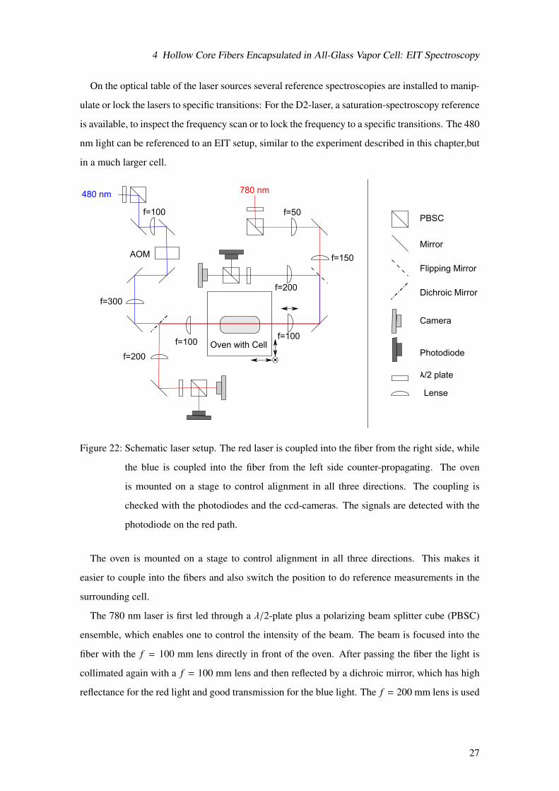
4 Hollow Core Fibers Encapsulated in All-Glass Vapor Cell: EIT Spectroscopy
On the optical table of the laser sources several reference spectroscopies are installed to manip-
ulate or lock the lasers to specific transitions: For the D2-laser, a saturation-spectroscopy reference
is available, to inspect the frequency scan or to lock the frequency to a specific transitions. The 480
nm light can be referenced to an EIT setup, similar to the experiment described in this chapter,but
in a much larger cell.
780 nm480 nm
PBSC
Mirror
Flipping Mirror
Dichroic Mirror
Oven with Cell
Camera
Photodiode
/2 plate
Lense
f=200
f=100
f=100
f=200
f=50
f=150AOM
f=100
f=300
Figure 22: Schematic laser setup. The red laser is coupled into the fiber from the right side, while
the blue is coupled into the fiber from the left side counter-propagating. The oven
is mounted on a stage to control alignment in all three directions. The coupling is
checked with the photodiodes and the ccd-cameras. The signals are detected with the
photodiode on the red path.
The oven is mounted on a stage to control alignment in all three directions. This makes it
easier to couple into the fibers and also switch the position to do reference measurements in the
surrounding cell.
The 780 nm laser is first led through a λ/2-plate plus a polarizing beam splitter cube (PBSC)
ensemble, which enables one to control the intensity of the beam. The beam is focused into the
fiber with the f = 100 mm lens directly in front of the oven. After passing the fiber the light is
collimated again with a f = 100 mm lens and then reflected by a dichroic mirror, which has high
reflectance for the red light and good transmission for the blue light. The f = 200 mm lens is used
27
4 Hollow Core Fibers Encapsulated in All-Glass Vapor Cell: EIT Spectroscopy
to enlarge the image of the end of the fiber and project it onto the ccd-camera. The coupling is
optimized through visual confirmation of the mode form and also of the transmitted power checked
with the photodiode. Later this photodiode is also used to record the absorption spectra as well as
the EIT signal.
The blue 480 nm beam is set up similarly to the red beam but coupled into the fiber counter-
propagating. There are only two differences: Behind the oven, instead of a dichroic mirror a
flipping mirror is used since this part of the beam is only needed for the coupling process.
Additionally, the first f = 100 mm lens is used to focus the beam into an acoustic optical modulator
(AOM). It is set up such that if the AOM is switched on, 80% of the light gets transmitted in the
first mode. Through this method the strength of the blue beam coupled into the fiber can be
modulated and a lock-in-amplifier can be used.
4.2 Results
4.2.1 Optical Density
The characterization of the system in comparison to the conventional system containing a vacuum-
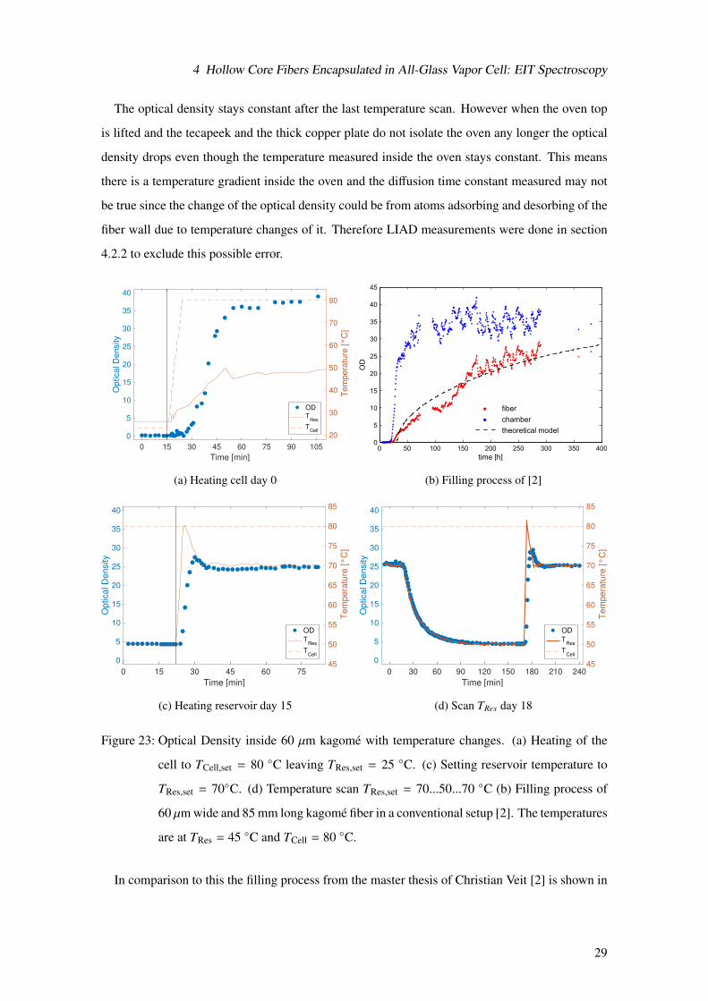
chamber and pump is of great interest. In figure (23) the filling process for the 60 µm kagome fiber
is shown. The cell had been filled with rubidium half a year ago and stored at room-temperature
before the cell was heated for the first time. In figure (23a) the measurement of the optical density
inside the fiber while heating the cell can be seen. At t = 15 min the temperature of the cell is
set to TCell,Set = 80 C. As mentioned the reservoir and the cell are not completely temperature
independent, therefore even though the set reservoir temperature is left at TRes,Set = 25 C it rises
with some delay. In response the optical density begins to rise at t = 26 min and saturates after
approximately 20 min at a mean value of 36.9. But over the course of the next four to five days the
optical density inside the fiber drops again until it stabilizes at a mean density of 5.8. This is best
explained by the fact, that the sample hat been stored at room temperature for half a year and the
rubidium atoms had time to diffuse into the fiber and get absorbed at the wall of the whole cell.
There were also rubidium droplets inside the cell which now evaporated, leading to a fast rise of
the density inside the cell and a slow equilibration of the system.
After two weaks, when the optical density was assumed to be stable, the reservoir temperature is
risen to TRes,set = 70 C as can be seen in figure (23c). The optical density reaches its maximum 6
minutes after the temperature was set. This implies a fast reaction of the system to the temperature
change and a diffusion time constant in the regime of minutes. In figure (23d) this is verified when
the graph of the optical density and the reservoir temperature show a very good overlap.
28
4 Hollow Core Fibers Encapsulated in All-Glass Vapor Cell: EIT Spectroscopy
The optical density stays constant after the last temperature scan. However when the oven top
is lifted and the tecapeek and the thick copper plate do not isolate the oven any longer the optical
density drops even though the temperature measured inside the oven stays constant. This means
there is a temperature gradient inside the oven and the diffusion time constant measured may not
be true since the change of the optical density could be from atoms adsorbing and desorbing of the
fiber wall due to temperature changes of it. Therefore LIAD measurements were done in section
4.2.2 to exclude this possible error.
0 15 30 45 60 75 90 105
Time [min]
0
5
10
15
20
25
30
35
40
Optical D
ensity
20
30
40
50
60
70
80
Tem
pera
ture
[°
C]
OD
TRes
TCell
(a) Heating cell day 0
laser detuning
transm
issio
n
(b) Filling process of [2]
0 15 30 45 60 75
Time [min]
0
5
10
15
20
25
30
35
40
Optical D
ensity
45
50
55
60
65
70
75
80
85
Tem
pera
ture
[°
C]
OD
TRes
TCell
(c) Heating reservoir day 15
0 30 60 90 120 150 180 210 240
Time [min]
0
5
10
15
20
25
30
35
40
Optical D
ensity
45
50
55
60
65
70
75
80
85
Tem
pera
ture
[°
C]
OD
TRes
TCell
(d) Scan TRes day 18
Figure 23: Optical Density inside 60 µm kagome with temperature changes. (a) Heating of the
cell to TCell,set = 80 C leaving TRes,set = 25 C. (c) Setting reservoir temperature to
TRes,set = 70C. (d) Temperature scan TRes,set = 70...50...70 C (b) Filling process of
60 µm wide and 85 mm long kagome fiber in a conventional setup [2]. The temperatures
are at TRes = 45 C and TCell = 80 C.
In comparison to this the filling process from the master thesis of Christian Veit [2] is shown in
29
4 Hollow Core Fibers Encapsulated in All-Glass Vapor Cell: EIT Spectroscopy
figure (23b) (note that the time-scale differs by a factor of 100). In this thesis the setup consists of
a conventional vacuum-chamber with the fibers mounted inside and a cesium reservoir. The fiber
had a length of 85 mm and an inner diameter of 60 µm . At t = 0 the reservoir and the cell are
heated to TRes = 45 C and TCell = 80 C respectively. In the first 10 hours no cesium can be
detected, most likely because of the cesium atoms depositing on the wall surfaces of the vacuum
chamber. But after that delay the optical density rises quickly inside the chamber and the optical
density inside the fiber follows. Noticeable is here, that the time scale of the diffusion process into
the fiber is in the regime of hours whereas in the case of the current thesis process happens within
minutes. To explain this some facts have to be taken into account.
In [2] the fiber is first exposed to cesium at the time t = 10 h and from there a curing process takes
place, where the atoms adsorbe on the surface and then diffuse into the glass bulk of the fiber.
Therefore the atoms indeed diffuse into the fiber but do not contribute to a rise in atomic density
in the fiber core. In the present thesis this curing process could not be observed due to various
reasons. First of all the fiber was first exposed to the rubidium vapor during the filling process
of the cell, when the cell was still connected to the vacuum pump and not in the optical set up.
Secondly when the cell was ablated from the vacuum setup the optical setup was not ready yet
since at that time the setup for the fiber series was installed first. So the fiber had enough time to
go through the curing process.
Nevertheless the fiber cell holds some advantages in comparison to the conventional vacuum-
chamber. Except for the (one time) filling process it gets by without a big vacuum setup. And the
vacuum setup can be used to fill multiple cells with different fiber types with minimal cleaning
effort of the vacuum parts. These cells can then easily be brought into the optical setup. Switching
times between fibers are only limited to the time it takes to open and close the oven and to couple
into the new fiber. If the cells are standardizes in respect to the fiber position inside the cell, the
coupling time can be reduces drastically.
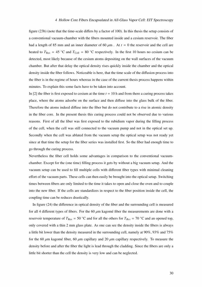
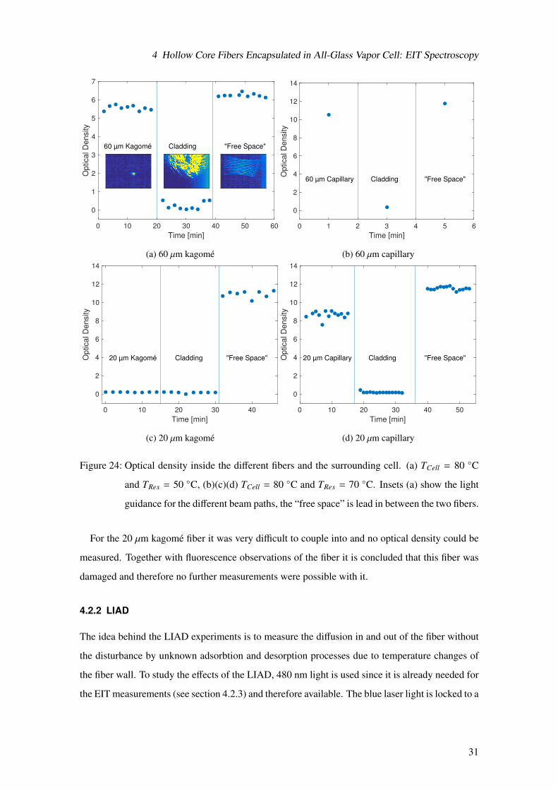
In figure (24) the difference in optical density of the fiber and the surrounding cell is measured
for all 4 different types of fibers. For the 60 µm kagome fiber the measurements are done with a
reservoir temperature of TRes = 50 C and for all the others for TRes = 70 C and an opened top,
only covered with a thin 2 mm glass plate. As one can see the density inside the fibers is always
a little bit lower than the density measured in the surrounding cell, namely at 90%, 93% and 75%
for the 60 µm kagome fiber, 60 µm capillary and 20 µm capillary respectively. To measure the
density before and after the fiber the light is lead through the cladding. Since the fibers are only a
little bit shorter than the cell the density is very low and can be neglected.
30
4 Hollow Core Fibers Encapsulated in All-Glass Vapor Cell: EIT Spectroscopy
0 10 20 30 40 50 60
Time [min]
0
1
2
3
4
5
6
7O
ptical D
ensity
60 µm Kagomé "Free Space"Cladding
(a) 60 µm kagome
0 1 2 3 4 5 6
Time [min]
0
2
4
6
8
10
12
14
Optical D
ensity
60 µm Capillary Cladding "Free Space"
(b) 60 µm capillary
0 10 20 30 40
Time [min]
0
2
4
6
8
10
12
14
Op
tica
l D
en
sity
20 µm Kagomé "Free Space"Cladding
(c) 20 µm kagome
0 10 20 30 40 50
Time [min]
0
2
4
6
8
10
12
14
Op
tica
l D
en
sity
20 µm Capillary "Free Space"Cladding
(d) 20 µm capillary
Figure 24: Optical density inside the different fibers and the surrounding cell. (a) TCell = 80 C
and TRes = 50 C, (b)(c)(d) TCell = 80 C and TRes = 70 C. Insets (a) show the light
guidance for the different beam paths, the “free space” is lead in between the two fibers.
For the 20 µm kagome fiber it was very difficult to couple into and no optical density could be
measured. Together with fluorescence observations of the fiber it is concluded that this fiber was
damaged and therefore no further measurements were possible with it.
4.2.2 LIAD
The idea behind the LIAD experiments is to measure the diffusion in and out of the fiber without
the disturbance by unknown adsorbtion and desorption processes due to temperature changes of
the fiber wall. To study the effects of the LIAD, 480 nm light is used since it is already needed for
the EIT measurements (see section 4.2.3) and therefore available. The blue laser light is locked to a
31
4 Hollow Core Fibers Encapsulated in All-Glass Vapor Cell: EIT Spectroscopy
cavity at a frequency off-resonant to any transition to avoid distortion of the density measurements
due to optical pumping or EIT effects. The optical density is monitored with the 780 nm light
like before.
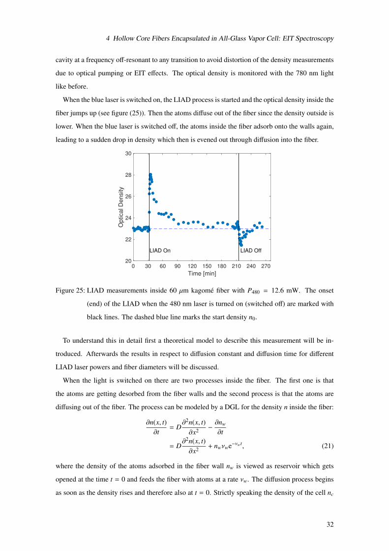
When the blue laser is switched on, the LIAD process is started and the optical density inside the
fiber jumps up (see figure (25)). Then the atoms diffuse out of the fiber since the density outside is
lower. When the blue laser is switched off, the atoms inside the fiber adsorb onto the walls again,
leading to a sudden drop in density which then is evened out through diffusion into the fiber.
0 30 60 90 120 150 180 210 240 270
Time [min]
20
22
24
26
28
30
Optical D
ensity
LIAD On LIAD Off
Figure 25: LIAD measurements inside 60 µm kagome fiber with P480 = 12.6 mW. The onset
(end) of the LIAD when the 480 nm laser is turned on (switched off) are marked with
black lines. The dashed blue line marks the start density n0.
To understand this in detail first a theoretical model to describe this measurement will be in-
troduced. Afterwards the results in respect to diffusion constant and diffusion time for different
LIAD laser powers and fiber diameters will be discussed.
When the light is switched on there are two processes inside the fiber. The first one is that
the atoms are getting desorbed from the fiber walls and the second process is that the atoms are
diffusing out of the fiber. The process can be modeled by a DGL for the density n inside the fiber:
∂n(x, t)∂t
= D∂2n(x, t)∂x2 −
∂nw
∂t
= D∂2n(x, t)∂x2 + nwνwe−νwt, (21)
where the density of the atoms adsorbed in the fiber wall nw is viewed as reservoir which gets
opened at the time t = 0 and feeds the fiber with atoms at a rate νw. The diffusion process begins
as soon as the density rises and therefore also at t = 0. Strictly speaking the density of the cell nc
32
4 Hollow Core Fibers Encapsulated in All-Glass Vapor Cell: EIT Spectroscopy
outside the fiber should rise because of the atoms diffusing outside, but since the volume of the cell
is much larger than the fiber, nc can be approximated to be constant throughout the measurement.
The density n should equilibrate to the same value as before the LIAD. This leads to the boundary
conditions for a fiber of length l of:
n(x, t = 0) = n0 for − l/2 ≤ x ≤ l/2 (22)
n(x = ±l/2, t) = n0. (23)
With this the numerical solution for eq. (21) can be computed. In the case of switching off the
blue light, only the sign in front of the desorption term changes in eq. (21). Now the wall is seen
as a drain and nw is the density of atoms getting absorbed into the fiber wall with the rate νw. Since
the optical density is proportional to the atomic density, this simulation can be transferred directly
to the measurements.
50 100 150
Time [min]
22
23
24
25
26
27
28
29
Optical D
ensity
t85%
= 51.76 min
OD
Theory
(a) P480 = 12.6 mW
50 100 150
Time [min]
22
23
24
25
26
27
28
29
Optical D
ensity
t85%
= 59.23 min
OD
Theory
(b) P480 = 12.6 mW
0 50 100 150 200
Time [min]
22
23
24
25
26
27
28
29
Op
tica
l D
en
sity
t85%
= 49.35 min
OD
Theory
(c) P480 = 6.3 mW
210 220 230 240 250 260
Time [min]
21
21.5
22
22.5
23
23.5
24
24.5
Optical D
ensity
t85%
= 39.90 min
OD
Theory
(d) P480 = 12.6 mW
220 240 260 280 300 320 340
Time [min]
21
21.5
22
22.5
23
23.5
24
24.5
Optical D
ensity
t85%
= 36.69 min
OD
Theory
(e) P480 = 12.6 mW
210 220 230 240 250 260 270
Time [min]
21
21.5
22
22.5
23
23.5
24
24.5
Optical D
ensity
t85%
= 25.86 min
OD
Theory
(f) P480 = 6.3 mW
Figure 26: LIAD measurements in 60 µm kagome fiber for different blue laser powers. The blue
dashed line marks the start density n0 and the end density used for the simulations.
Except for case (e) start and end density are the same. In (e) the system was not equili-
brated again before the laser was turned off leading to a higher start density.
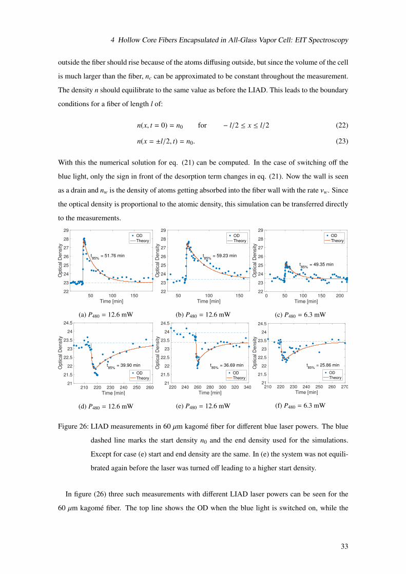
In figure (26) three such measurements with different LIAD laser powers can be seen for the
60 µm kagome fiber. The top line shows the OD when the blue light is switched on, while the
33
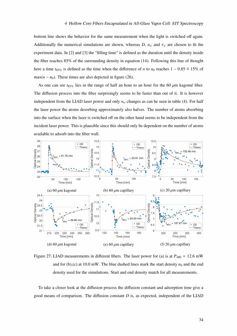
4 Hollow Core Fibers Encapsulated in All-Glass Vapor Cell: EIT Spectroscopy
bottom line shows the behavior for the same measurement when the light is switched off again.
Additionally the numerical simulations are shown, whereas D, nw and τw are chosen to fit the
experiment data. In [2] and [3] the “filling time” is defined as the duration until the density inside
the fiber reaches 85% of the surrounding density in equation (14). Following this line of thought
here a time t85% is defined as the time when the difference of n to n0 reaches 1 − 0.85 = 15% of
max(n − n0). These times are also depicted in figure (26).
As one can see t85% lies in the range of half an hour to an hour for the 60 µm kagome fiber.
The diffusion process into the fiber surprisingly seems to be faster than out of it. It is however
independent from the LIAD laser power and only nw changes as can be seen in table (4). For half
the laser power the atoms desorbing approximately also halves. The number of atoms absorbing
into the surface when the laser is switched off on the other hand seems to be independent from the
incident laser power. This is plausible since this should only be dependent on the number of atoms
available to adsorb into the fiber wall.
50 100 150
Time [min]
22
23
24
25
26
27
28
29
Optical D
ensity
t85%
= 51.76 min
OD
Theory
(a) 60 µm kagome
0 50 100
Time [min]
10.5
11
11.5
12
12.5
13
13.5
Optical D
ensity
t85%
= 23.91 min
OD
Theory
(b) 60 µm capillary
0 50 100 150
Time [min]
7.5
8
8.5
9
9.5
10
10.5
Optical D
ensity
t85%
= 152.48 min
OD
Theory
(c) 20 µm capillary
210 220 230 240 250 260
Time [min]
21
21.5
22
22.5
23
23.5
24
24.5
Optical D
ensity
t85%
= 39.90 min
OD
Theory
(d) 60 µm kagome
120 140 160 180
Time [min]
9.5
10
10.5
11
11.5
12
Optical D
ensity
t85%
= 24.93 min
OD
Theory
(e) 60 µm capillary
200 250 300 350
Time [min]
6
6.5
7
7.5
8
8.5
9
Optical D
ensity
t85%
= 187.67 minOD
Theory
(f) 20 µm capillary
Figure 27: LIAD measurements in different fibers. The laser power for (a) is at P480 = 12.6 mW
and for (b),(c) at 10.0 mW. The blue dashed lines mark the start density n0 and the end
density used for the simulations. Start and end density match for all measurements.
To take a closer look at the diffusion process the diffusion constant and adsorption time give a
good means of comparison. The diffusion constant D is, as expected, independent of the LIAD
34
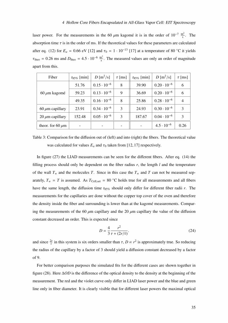
4 Hollow Core Fibers Encapsulated in All-Glass Vapor Cell: EIT Spectroscopy
laser power. For the measurements in the 60 µm kagome it is in the order of 10−7 m2
s . The
absorption time τ is in the order of ms. If the theoretical values for these parameters are calculated
after eq. (12) for Ea = 0.66 eV [12] and τ0 = 1 · 10−13 [17] at a temperature of 80 C it yields
τtheo = 0.26 ms and Dtheo = 4.5 · 10−6 m2
s . The measured values are only an order of magnitude
apart from this.
Fiber t85% [min] D [m2/s] τ [ms] t85% [min] D [m2/s] τ [ms]
51.76 0.15 · 10−6 8 39.90 0.20 · 10−6 6
60 µm kagome 59.23 0.13 · 10−6 9 36.69 0.20 · 10−6 6
49.35 0.16 · 10−6 8 25.86 0.28 · 10−6 4
60 µm capillary 23.91 0.34 · 10−6 3 24.93 0.30 · 10−6 3
20 µm capillary 152.48 0.05 · 10−6 3 187.67 0.04 · 10−6 3
theor. for 60 µm - - - - 4.5 · 10−6 0.26
Table 3: Comparison for the diffusion out of (left) and into (right) the fibers. The theoretical value
was calculated for values Ea and τ0 taken from [12, 17] respectively.
In figure (27) the LIAD measurements can be seen for the different fibers. After eq. (14) the
filling process should only be dependent on the fiber radius r, the length l and the temperature
of the wall Tw and the molecules T . Since in this case the Tw and T can not be measured sep-
arately, Tw = T is assumed. As TCell,set = 80 C holds true for all measurements and all fibers
have the same length, the diffusion time t85% should only differ for different fiber radii r. The
measurements for the capillaries are done without the copper top cover of the oven and therefore
the density inside the fiber and surrounding is lower than at the kagome measurements. Compar-
ing the measurements of the 60 µm capillary and the 20 µm capillary the value of the diffusion
constant decreased an order. This is expected since
D =43
r2
τ + (2r/v). (24)
and since 2rv in this system is six orders smaller than τ, D ∝ r2 is approximately true. So reducing
the radius of the capillary by a factor of 3 should yield a diffusion constant decreased by a factor
of 9.
For better comparison purposes the simulated fits for the different cases are shown together in
figure (28). Here ∆OD is the difference of the optical density to the density at the beginning of the
measurement. The red and the violet curve only differ in LIAD laser power and the blue and green
line only in fiber diameter. It is clearly visible that for different laser powers the maximal optical
35
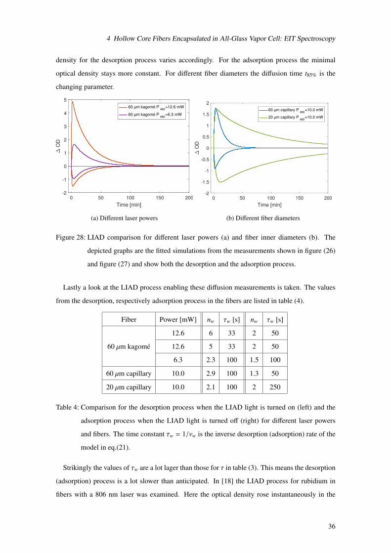
4 Hollow Core Fibers Encapsulated in All-Glass Vapor Cell: EIT Spectroscopy
density for the desorption process varies accordingly. For the adsorption process the minimal
optical density stays more constant. For different fiber diameters the diffusion time t85% is the
changing parameter.
0 50 100 150 200
Time [min]
-2
-1
0
1
2
3
4
5
∆ O
D
60 µm kagomé P480
=12.6 mW
60 µm kagomé P480
=6.3 mW
(a) Different laser powers
0 50 100 150 200
Time [min]
-2
-1.5
-1
-0.5
0
0.5
1
1.5
2
∆ O
D
60 µm capillary P480
=10.0 mW
20 µm capillary P480
=10.0 mW
(b) Different fiber diameters
Figure 28: LIAD comparison for different laser powers (a) and fiber inner diameters (b). The
depicted graphs are the fitted simulations from the measurements shown in figure (26)
and figure (27) and show both the desorption and the adsorption process.
Lastly a look at the LIAD process enabling these diffusion measurements is taken. The values
from the desorption, respectively adsorption process in the fibers are listed in table (4).
Fiber Power [mW] nw τw [s] nw τw [s]
12.6 6 33 2 50
60 µm kagome 12.6 5 33 2 50
6.3 2.3 100 1.5 100
60 µm capillary 10.0 2.9 100 1.3 50
20 µm capillary 10.0 2.1 100 2 250
Table 4: Comparison for the desorption process when the LIAD light is turned on (left) and the
adsorption process when the LIAD light is turned off (right) for different laser powers
and fibers. The time constant τw = 1/νw is the inverse desorption (adsorption) rate of the
model in eq.(21).
Strikingly the values of τw are a lot lager than those for τ in table (3). This means the desorption
(adsorption) process is a lot slower than anticipated. In [18] the LIAD process for rubidium in
fibers with a 806 nm laser was examined. Here the optical density rose instantaneously in the
36
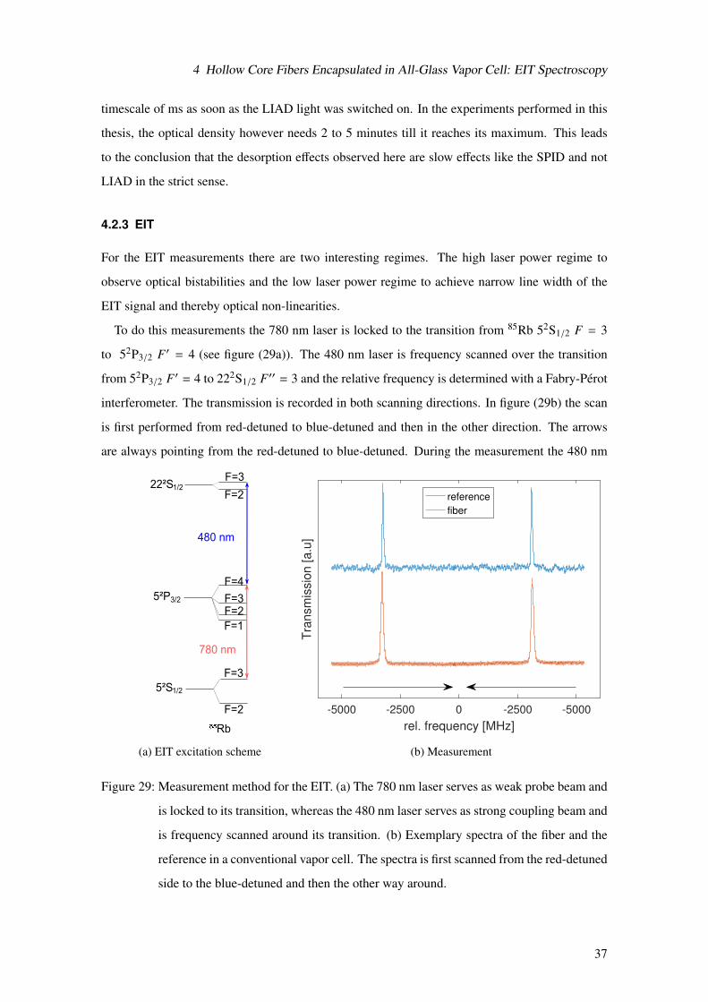
4 Hollow Core Fibers Encapsulated in All-Glass Vapor Cell: EIT Spectroscopy
timescale of ms as soon as the LIAD light was switched on. In the experiments performed in this
thesis, the optical density however needs 2 to 5 minutes till it reaches its maximum. This leads
to the conclusion that the desorption effects observed here are slow effects like the SPID and not
LIAD in the strict sense.
4.2.3 EIT
For the EIT measurements there are two interesting regimes. The high laser power regime to
observe optical bistabilities and the low laser power regime to achieve narrow line width of the
EIT signal and thereby optical non-linearities.
To do this measurements the 780 nm laser is locked to the transition from 85Rb 52S1/2 F = 3
to 52P3/2 F′ = 4 (see figure (29a)). The 480 nm laser is frequency scanned over the transition
from 52P3/2 F′ = 4 to 222S1/2 F′′ = 3 and the relative frequency is determined with a Fabry-Perot
interferometer. The transmission is recorded in both scanning directions. In figure (29b) the scan
is first performed from red-detuned to blue-detuned and then in the other direction. The arrows
are always pointing from the red-detuned to blue-detuned. During the measurement the 480 nm
5²S1/2
Rb
F=2
F=3
5²P3/2
F=2
F=3
F=4
F=1
780 nm
22²S1/2
480 nm
F=2
F=3
(a) EIT excitation scheme
-5000 -2500 0 -2500 -5000
rel. frequency [MHz]
Tra
nsm
issio
n [a.u
]
reference
fiber
(b) Measurement
Figure 29: Measurement method for the EIT. (a) The 780 nm laser serves as weak probe beam and
is locked to its transition, whereas the 480 nm laser serves as strong coupling beam and
is frequency scanned around its transition. (b) Exemplary spectra of the fiber and the
reference in a conventional vapor cell. The spectra is first scanned from the red-detuned
side to the blue-detuned and then the other way around.
37
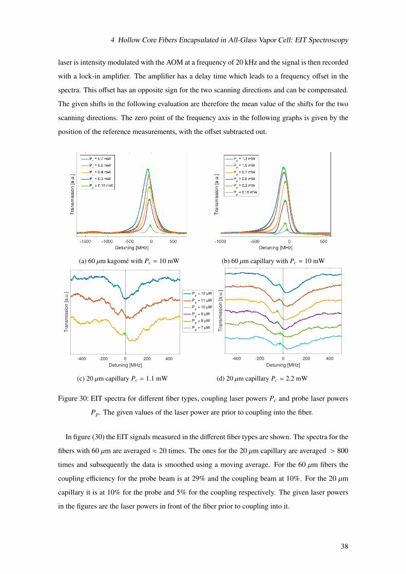
4 Hollow Core Fibers Encapsulated in All-Glass Vapor Cell: EIT Spectroscopy
laser is intensity modulated with the AOM at a frequency of 20 kHz and the signal is then recorded
with a lock-in amplifier. The amplifier has a delay time which leads to a frequency offset in the
spectra. This offset has an opposite sign for the two scanning directions and can be compensated.
The given shifts in the following evaluation are therefore the mean value of the shifts for the two
scanning directions. The zero point of the frequency axis in the following graphs is given by the
position of the reference measurements, with the offset subtracted out.
(a) 60 µm kagome with Pc = 10 mW (b) 60 µm capillary with Pc = 10 mW
-400 -200 0 200 400
Detuning [MHz]
Tra
nsm
issio
n [
a.u
.]
(c) 20 µm capillary Pc = 1.1 mW
-400 -200 0 200 400
Detuning [MHz]
Tra
nsm
issio
n [a.u
.]Pp = 12 µW
Pp = 11 µW
Pp = 10 µW
Pp = 9 µW
Pp = 8 µW
Pp = 7 µW
(d) 20 µm capillary Pc = 2.2 mW
Figure 30: EIT spectra for different fiber types, coupling laser powers Pc and probe laser powers
Pp. The given values of the laser power are prior to coupling into the fiber.
In figure (30) the EIT signals measured in the different fiber types are shown. The spectra for the
fibers with 60 µm are averaged ≈ 20 times. The ones for the 20 µm capillary are averaged > 800
times and subsequently the data is smoothed using a moving average. For the 60 µm fibers the
coupling efficiency for the probe beam is at 29% and the coupling beam at 10%. For the 20 µm
capillary it is at 10% for the probe and 5% for the coupling respectively. The given laser powers
in the figures are the laser powers in front of the fiber prior to coupling into it.
38
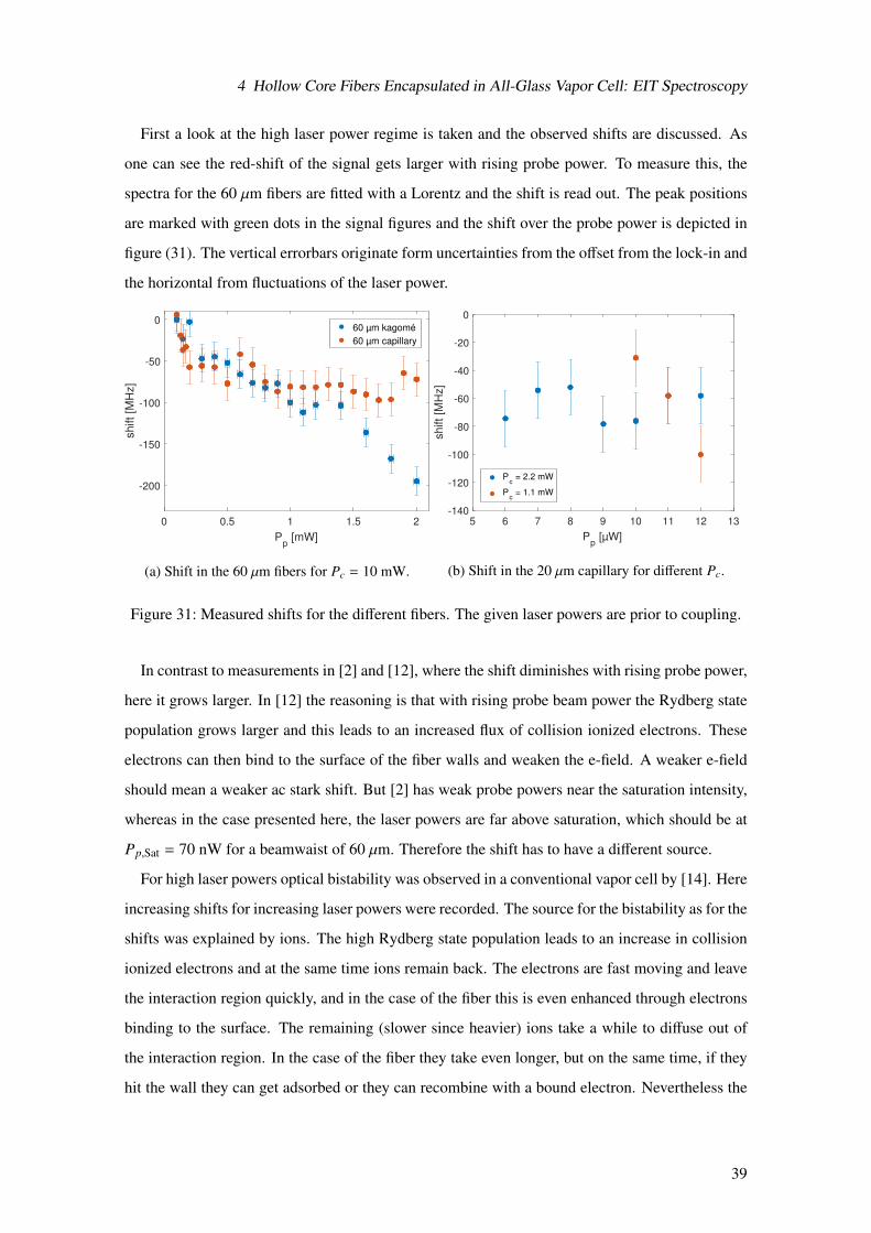
4 Hollow Core Fibers Encapsulated in All-Glass Vapor Cell: EIT Spectroscopy
First a look at the high laser power regime is taken and the observed shifts are discussed. As
one can see the red-shift of the signal gets larger with rising probe power. To measure this, the
spectra for the 60 µm fibers are fitted with a Lorentz and the shift is read out. The peak positions
are marked with green dots in the signal figures and the shift over the probe power is depicted in
figure (31). The vertical errorbars originate form uncertainties from the offset from the lock-in and
the horizontal from fluctuations of the laser power.
0 0.5 1 1.5 2
Pp [mW]
-200
-150
-100
-50
0
shift [M
Hz]
60 µm kagomé
60 µm capillary
(a) Shift in the 60 µm fibers for Pc = 10 mW.
5 6 7 8 9 10 11 12 13
Pp [µW]
-140
-120
-100
-80
-60
-40
-20
0
shift [M
Hz]
Pc = 2.2 mW
Pc = 1.1 mW
(b) Shift in the 20 µm capillary for different Pc.
Figure 31: Measured shifts for the different fibers. The given laser powers are prior to coupling.
In contrast to measurements in [2] and [12], where the shift diminishes with rising probe power,
here it grows larger. In [12] the reasoning is that with rising probe beam power the Rydberg state
population grows larger and this leads to an increased flux of collision ionized electrons. These
electrons can then bind to the surface of the fiber walls and weaken the e-field. A weaker e-field
should mean a weaker ac stark shift. But [2] has weak probe powers near the saturation intensity,
whereas in the case presented here, the laser powers are far above saturation, which should be at
Pp,Sat = 70 nW for a beamwaist of 60 µm. Therefore the shift has to have a different source.
For high laser powers optical bistability was observed in a conventional vapor cell by [14]. Here
increasing shifts for increasing laser powers were recorded. The source for the bistability as for the
shifts was explained by ions. The high Rydberg state population leads to an increase in collision
ionized electrons and at the same time ions remain back. The electrons are fast moving and leave
the interaction region quickly, and in the case of the fiber this is even enhanced through electrons
binding to the surface. The remaining (slower since heavier) ions take a while to diffuse out of
the interaction region. In the case of the fiber they take even longer, but on the same time, if they
hit the wall they can get adsorbed or they can recombine with a bound electron. Nevertheless the
39
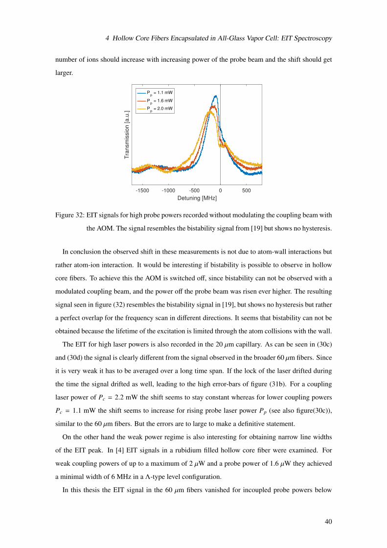
4 Hollow Core Fibers Encapsulated in All-Glass Vapor Cell: EIT Spectroscopy
number of ions should increase with increasing power of the probe beam and the shift should get
larger.
-1500 -1000 -500 0 500
Detuning [MHz]
Tra
nsm
issio
n [a.u
.]
Pp = 1.1 mW
Pp = 1.6 mW
Pp = 2.0 mW
Figure 32: EIT signals for high probe powers recorded without modulating the coupling beam with
the AOM. The signal resembles the bistability signal from [19] but shows no hysteresis.
In conclusion the observed shift in these measurements is not due to atom-wall interactions but
rather atom-ion interaction. It would be interesting if bistability is possible to observe in hollow
core fibers. To achieve this the AOM is switched off, since bistability can not be observed with a
modulated coupling beam, and the power off the probe beam was risen ever higher. The resulting
signal seen in figure (32) resembles the bistability signal in [19], but shows no hysteresis but rather
a perfect overlap for the frequency scan in different directions. It seems that bistability can not be
obtained because the lifetime of the excitation is limited through the atom collisions with the wall.
The EIT for high laser powers is also recorded in the 20 µm capillary. As can be seen in (30c)
and (30d) the signal is clearly different from the signal observed in the broader 60 µm fibers. Since
it is very weak it has to be averaged over a long time span. If the lock of the laser drifted during
the time the signal drifted as well, leading to the high error-bars of figure (31b). For a coupling
laser power of Pc = 2.2 mW the shift seems to stay constant whereas for lower coupling powers
Pc = 1.1 mW the shift seems to increase for rising probe laser power Pp (see also figure(30c)),
similar to the 60 µm fibers. But the errors are to large to make a definitive statement.
On the other hand the weak power regime is also interesting for obtaining narrow line widths
of the EIT peak. In [4] EIT signals in a rubidium filled hollow core fiber were examined. For
weak coupling powers of up to a maximum of 2 µW and a probe power of 1.6 µW they achieved
a minimal width of 6 MHz in a Λ-type level configuration.
In this thesis the EIT signal in the 60 µm fibers vanished for incoupled probe powers below
40
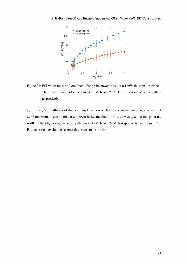
4 Hollow Core Fibers Encapsulated in All-Glass Vapor Cell: EIT Spectroscopy
0 0.5 1 1.5 2
Pp [mW]
0
50
100
150
200
250
Wid
th [
MH
z]
60 µm kagomé
60 µm capillary
Figure 33: EIT width for the 60 µm fibers. For probe powers smaller 0.1 mW the signal vanished.
The smallest width observed are at 33 MHz and 27 MHz for the kagome and capillary
respectively.
Pp = 100 µW indifferent of the coupling laser power. For the achieved coupling efficiency of
29 % this would mean a probe laser power inside the fiber of Pp,inside = 28 µW. At this point the
width for the 60 µm kagome and capillary is at 33 MHz and 27 MHz respectively (see figure (33)).
For the present excitation scheme this seems to be the limit.
41
5 Conclusion and Outlook
5 Conclusion and Outlook
The aim of this thesis was to gain further insight into the combination of Rydberg spectroscopy
in atomic vapor with hollow core optical fibers. Therefore, two different sample types of hollow
core fibers were examined. One was the fiber series and the other a conventional vapor cell with
two hollow core fibers mounted inside.
The fiber series is a step towards miniaturized optical devices for electromagnetic field measure-
ments. The setup of a single-mode optical fiber placed in series with a glass capillary followed
by a multi-mode optical fiber had a transmission efficiency of 4.4% respectively 6.6% for the
single-mode to multi-mode transmission direction, which is in the expected regime of ≈ 5%. In
the reverse direction, the transmission was lower, namely at 0.01% and 0.03% respectively, but
still non-zero. Absorption spectroscopy measurements could be done in both directions, but sub-
doppler spectroscopy proved to be challenging due to an interference signal of unknown origin
for light traveling in the multi-mode to single-mode direction. Measurements with co-propagating
beams in the single-mode to multi-mode direction lead to strongly broadened “Lamb dips”. The
broadening is most likely due to pressure broadening effects.
Nevertheless the principle of the device is proven to be working. Additional measurements
should be done with different samples to clarify the origin of the interference signal and the broad-
ening mechanism for the sub-doppler regime.
The second sample type consists of a capillary and a hollow core kagome photonic crystal fiber,
both mounted in a conventional all glass vapor cell. They each had the same inner-diameter. Two
of these samples were prepared, one with fibers of a inner-diameter of 60 µm and the other with
20 µm. LIAD measurements inside this fibers showed that the diffusion process is strongly de-
pendent on the core diameter, with smaller core sizes leading to longer diffusion times. For the
60 µm fibers the diffusion constants were in the order of 10−7 m2
s . Predictions from theoretical cal-
culations lead to diffusion constants in the order of 10−6 m2
s , which is only one order of magnitude
apart. The measured diffusion constant for the 20 µm fibers was at the order of 10−8 m2
s . Like it
was expected it is an order smaller than the diffusion in the 3 times wider fibers.
Finally EIT measurements with counter-propagating probe and coupling beams were performed.
For high laser powers the signal showed a red-shift which is contributed to collision ionization
of the Rydberg states. These ions interact with the Rydberg atoms and produce a energy shift
which rises with increasing ion population. The search for a bistability signal resulting from those
Rydberg-ion interactions lead to no finding. This is most likely contributed to the fact that the
42
5 Conclusion and Outlook
bistable states can not be sustained long enough due to collisions with the fiber wall. For weaker
laser powers the width of the signal was observed in order to evaluate the feasibility of non-linear
optics. There was a lower limit of the probe beam power under which the EIT signal vanished. At
this point the width was in the range of 30 MHz. Further measurements should be conducted so
examine what steps have to be taken to reduce this line width further. For example reducing the
atomic density inside the fibers could lead to EIT signals with lower laser powers.
Nevertheless the results for the two different fiber samples showed that bulky vacuum-chambers
are no longer necessary and an important step in the direction of generating miniaturized, inte-
grable, room-temperature devices was achieved.
43
Bibliography
Bibliography
[1] Rolf Heidemann, Ulrich Raitzsch, Vera Bendkowsky, Bjorn Butscher, Robert Low, Luis San-
tos, and Tilman Pfau. Evidence for coherent collective rydberg excitation in the strong block-
ade regime. Physical review letters, 99(16):163601, 2007.
[2] Christian Veit. Rf dressing of rydberg states in hollow-core fibers: Master thesis. Universitat
Stuttgart, 2015.
[3] Kathrin Kleinbach. Rydberg spectroscopy in hollow core fibers: Master thesis. Universitat
Stuttgart, 2014.
[4] P. S. Light, F. Benabid, F. Couny, M. Maric, and A. N. Luiten. Electromagnetically induced
transparency in rb-filled coated hollow-core photonic crystal fiber. Opt. Lett., 32(10):1323–
1325, 2007.
[5] Daniel A. Steck. Alkali D Line Data. Version 2.1.4. http://steck.us/alkalidata, 2010.
[6] Wolfgang Demtroder. Laserspektroskopie 1: Grundlagen. SpringerLink : Bucher. Springer-
Verlag Berlin Heidelberg, Berlin and Heidelberg, 6., aktualisierte auflage edition, 2011.
[7] Wolfgang Demtroder. Laserspektroskopie 2: Experimentelle Techniken. Springer, Berlin, 6.
neu bearbeitete und aktualisierte auflage edition, 2013.
[8] Rick K. Nubling. Launch conditions and mode coupling in hollow-glass waveguides. Optical
Engineering, 37(9):2454, 1998.
[9] G. J. Pearce, G. S. Wiederhecker, C. G. Poulton, S. Burger, and P. St. J. Russell. Mod-
els for guidance in kagome-structured hollow-core photonic crystal fibres. Optics Express,
15(20):12680, 2007.
[10] P. Clausing. Uber die adsorptionszeit und ihre messung durch stromungsversuche. Annalen
der Physik, 399(4):489–520, 1930.
[11] A. Burchianti, A. Bogi, C. Marinelli, C. Maibohm, E. Mariotti, S. Sanguinetti, and L. Moi.
Optical characterization and manipulation of alkali metal nanoparticles in porous silica. The
European Physical Journal D, 49(2):201–210, 2008.
[12] J. A. Sedlacek, E. Kim, S. T. Rittenhouse, P. F. Weck, H. R. Sadeghpour, and J. P. Shaf-
fer. Electric field cancellation on quartz by rb adsorbate-induced negative electron affinity.
Physical review letters, 116(13):133201, 2016.
44
Bibliography
[13] Michael Fleischhauer, Atac Imamoglu, and Jonathan P. Marangos. Electromagnetically in-
duced transparency: Optics in coherent media. Rev. Mod. Phys., 77(2):633–673, 2005.
[14] Daniel Weller, Alban Urvoy, Andy Rico, Robert Low, and Harald Kubler. Charge-induced
optical bistability in thermal rydberg vapor. Physical Review A, 94(6), 2016.
[15] C. Carr, R. Ritter, C. G. Wade, C. S. Adams, and K. J. Weatherill. Nonequilibrium phase
transition in a dilute rydberg ensemble. Physical review letters, 111(11):113901, 2013.
[16] Matthew Don Rotondaro. Collisional dynamics of the rubidium 52p levels: Dissertation.
1995.
[17] de Boer, J. H. The dynamical character of adsorption. Clarendon Press, Oxford, 1968.
[18] Amar R. Bhagwat, Aaron D. Slepkov, Vivek Venkataraman, Pablo Londero, and Alexan-
der L. Gaeta. On-demand all-optical generation of controlled rb-vapor densities in photonic-
band-gap fibers. Physical Review A, 79(6), 2009.
[19] D. S. Ding, C. S. Adams, B. S. Shi, G. C. Guo. Non-equilibrium phase-transitions in multi-
component rydberg gases. 2016.
45
Danksagung
Zuerst danke ich meinen Eltern, ohne die mir diese Studium nicht moglich gewesen ware und die
mich die ganzen letzten Jahre wunderbar und unubertrefflich unterstutzt haben.
Dann danke ich allen Mitarbeitern des Instituts und ganz besonders allen aus dem 3.Stock.
Fur all die vielen nutzlichen Ratschlage, Anregungen und Hilfestellungen die ihr mir das letzte
Jahr uber habt zukommen lassen. Ganz besonders danke ich Daniel Weller, der immer mit einer
helfenden Hand da war und mich sehr gut betreut hat. Vielen Dank auch fur das unermudliche
Korrekturlesen dieser Arbeit.
Nicht zuletzt bedanke ich mich bei meinen Freunden und Komilitonen, die immer da waren um
auch mal ein Problem auszudiskutieren, wenn ich einen Knoten im Kopf losen musste.
46