Electoral Control with Behavioral Voters

Daniel Diermeier�and Christopher Liy

Abstract

We present a model of electoral control with behavioral voters.

The model is intended to capture the main regularities of voting be-

havior found in empirical studies. Speci�cally, the voters�propensity

to keep an incumbent in o¢ ce is governed by a stochastic reinforce-

ment process instead of strategic reasoning. The likelihood of a pos-

itive feed-back for a voter depends on the e¤ort level exercised by the

public o¢ cial. We show that despite the lack of rational responses

by voters, the electoral control of public o¢ cials can be substantial.

Indeed, electoral control is the highest when voters are most forgetful.

Moreover, our model generates comparative statics that are consistent

with the main empirical regularities of electoral accountability.

JEL classi�cation: D03, D72, D83

Keywords: electoral control, adaptive behavioral voting, electoral account-

ability

�IBM Professor of Regulation and Competitive Practice, Department of ManagerialEconomics and Decision Sciences (MEDS), Kellogg School of Management, NorthwesternUniversity, 2001 Sheridan Rd., Evanston, IL. 60208, d-diermeier@kellogg.northwestern.eduand Canadian Institute for Advanced Research, CIFAR Program on Institutions, Organ-izations, and Growth, CIFAR, Toronto, ON M5G 1Z8.

yDepartment of Economics, Northwestern University, 2001 Sheridan Rd., Evanston, IL.60208, christopherli2015@u.northwestern.edu.

1 Introduction

The question of electoral control of public o¢ cials is of central concern in

political science. Some political theorists, e.g., Riker (1982; 9) following

Madison (Federalist 39), have even argued that democracy consists of the

control of public o¢ cials and little else. This has led to the question of how

well electoral accountability actually works. The formal political science

literature1 has focused on the e¤ect of asymmetric information on electoral

control.2 Some papers, like Barro (1973) and Ferejohn (1986), focus on moral

hazard, where the actions ("e¤ort") of the incumbent are unobservable and

the electorate chooses a retrospective voting rule to induce high e¤ort from

the incumbent. Other approaches, like Rogo¤ (1990) and Ashworth (2005),

consider the case of adverse selection, where the ability of the incumbent is

unknown and the electorate needs to screen out low ability incumbents. In a

typical model, the electorate and the incumbent interact in a dynamic game,

and the prediction is based on Nash Equilibrium. One of the main insights of

this literature is that some level of electoral accountability can be maintained

under informational asymmetry, albeit at a cost to the voters.3

In such models voters are assumed to be rational. They process information

as Bayesians and act strategically, and the game form is assumed to be com-

mon knowledge. This approach has been heavily criticized by political sci-

entists who empirically study voting behavior and public opinion. Concerns

go back to some of the early studies of voters conducted by the Columbia

and Michigan School (e.g. Berelson, Lazarsfeld and McPhee 1954, Campbell,

Converse, Miller, and Stokes 1960).

1See Ashworth (2012) for a recent overview2Under perfect information, the voters can trivially achieve complete electoral control

by conditioning reelection on the implementation of (voter) welfare maximizing policy.3In Rogo¤ (1990), for example, the voters can distinguish high ability incumbent from

low ability incumbent in a separating equilibrium, although the incumbent will implementin�ationary �scal policy, which is bad for welfare.

1

In his summary of post-war public opinion research, Stimson states (Stimson

2004; p. 13)

What those studies found was that ordinary Americans knew

almost nothing about public a¤airs and appeared to care about

issues as much as they knew: almost not at all. Their beliefs

were a scattering of unrelated ideas, often mutually contradictory.

Structure was nowhere to be found.

Recent research has further argued that not only do voters lack basic in-

formation or coherent policy positions, their reasoning processes are heavily

biased and bear no resemblance to Bayesian rationality (Achen and Bar-

tels 2004a). First, in evaluating the incumbent�s performance, voters rely

predominantly on the more recent events instead of the overall record (e.g.

Achen and Bartels 2004a, Bartels 2008, Bartels and Zaller 2001, Erickson

1989). Second, voters are a¤ected by irrelevant factors and events; they are

swayed by rhetoric, framing, and advertising and hold incumbents account-

able for events that are clearly beyond the o¢ ce holder�s control.4 One such

factor are facial features (Todorov et al. 2005, Bellew and Todorov 2007),

including facial similarities between candidates and voters (Bailenson et al.

2009). Another example are events that are clearly unrelated to the e¤orts of

candidates but nevertheless in�uence voters�attitudes. Studies have shown

that the voters� decision is a¤ected by shark attacks (Achen and Bartels

2004a), rainfall (Cole, Healy and Werker 2012, Gasper and Reeves 2011),

the global oil price (Wolfers 2007) and the success or failure of local college

football teams (Healy, Mo and Malhotra 2010).5

4These concerns not only apply to models with fully rational voters, but also accountsof "reasoning voters", where voters uses cues, endorsements by trusted parties, mediacoverage, debate performance etc. to make, while not fully rational, at least competentdecisions (e.g. Popkin 1991, Lupia and McCubbins 1998, Lau and Redlawsk 2006).

5Some external events do allow rational voters to deduce incumbent�s performance.For example, voter response will be in�uenced by disaster relief e¤orts (Cole, Healy, and

2

The aforementioned issues are particularly relevant in the domain of economic

voting. On the one hand, there is a large literature that documents the

correlation between favorable economic conditions and the reelection rates of

incumbents (e.g. Kramer 1971, Fair 1978, Lewis-Beck 1988, Erickson 1989,

Erickson 1990, Duch and Stevenson 2008). But establishing this correlation

by itself is not enough. For the standard principal-agent model to hold, voters

must be able to reward incumbents for good actions, but �lter out external

events ("luck") that are clearly beyond the incumbent�s control.

Wolfers (2007) provides evidence that this is not the case. Wolfers investig-

ates the impact of national economic conditions and the global oil price on

reelection rates for U.S. state governors. Consistent with previous studies

of economics voting, Wolfers (2007) shows that state economic performance

impacts gubernatorial reelection rates, but, crucially, he also shows that a

rise in oil prices has a positive e¤ect in oil producing states (such as Alaska,

Wyoming, and Texas), but a negative e¤ect on rust belt states which are net

consumers of oil (e.g. Michigan and Indiana). In other words, while gov-

ernors can do little to a¤ect global oil prices, they are still held accountable

by the voters.

The failure of rational information �ltering is not the only problem faced by

rational accounts of economic voting. As Hibbs (2006; p.570) has pointed out,

one implication of the principal-agent approach to electoral accountability is

that "the electorate should evaluate performance over the incumbent�s entire

term of o¢ ce, with little or no backward time discounting of performance

outcomes". In practice, however, much of the empirical economic voting

literature has used periods close to the election dates or overweighted recent

periods (e.g. Kramer 1971, Tufte 1978, Erickson 1989; Hibbs 2000; Bartels

and Zaller 2001). Achen and Bartels (2004a) argue that such restrictions

Werker 2011, Healy and Malhotra 2010, Gasper and Reeves 2011). The point is not thatthe incumbent�s performance (on the local economy or other matters of public importance,e.g. disaster management) has no e¤ect on reelection rates, but that rational voters shouldbe able to ignore irrelevant factors, but the evidence suggests that they aren�t.

3

are not an accident, but re�ect a fundamental feature of an electorate who

systematically ignores, discounts, or simply forgets relevant information that

occurred earlier in the term of an elected o¢ cial.6

The issues regarding voter sophistication have potentially important norm-

ative consequences for the assessment of democratic governance structures.

Arguments going as far back as Plato�s Republic have proclaimed that an

ill-informed and irrational public renders democracy unsuitable as a form of

government.7 A recent version of this criticism was formulated by Achen and

Bartels (2004b; p. 38):

Democratic government as practiced in the United States,

then, is a form of limited, random oligarchy. It is an oligarchy

because, year to year, the voters are not paying any attention and

thus have no say in what the government does. Only at election

time do they assess how they feel. At that point, the oligarchy

becomes random, because the choice between alternative govern-

ing teams often comes down to accidental and arbitrary criteria

such as droughts and recessions, which no government can a¤ect,

and aspects of the candidates�personal histories and personalities

6A separate line of argument, originally pointed out by Fearon (1999), has identi�eda tension between forward looking selection of good o¢ ce-holders and backward lookingstrategies that maximize incentives for o¢ ce-holders to engage in costly e¤ort (Alt, deMesquita and Rose 2011, Ashworth and de Mesquita 2008, Ashworth, de Mesquita andFriedenberg 2012). The election rule that selects good types may be di¤erent from theelection rule that maximized the o¢ ce-holder�s incentives to take costly action. There-fore, electoral control can increase if voters disregard some information about incumbents(Ashworth and de Mesquita 2013a). Ashworth and de Mesquita (2013b) show that in thepresence of both adverse selection and moral hazard, a rational retrospective voting ruledoes not necessarily maximize incentives for e¤ort nor ex-ante welfare. This leaves openthe possibility that a di¤erent (irrational) voting rule may induce higher e¤ort welfare.The results in our model are not driven by direct strategic interaction between voters andpoliticians since voters are non-strategic by de�nition. Moreover, we set aside issues ofincumbent quality and focus exclusively on electoral control as in the original Ferejohn(1986) model.

7For a discussion of this and related views see Dahl (1989).

4

with no relevance to the job.

In other words, the public control of o¢ cials does not function in an en-

vironment of an ignorant and uninterested public; electoral accountability

depends on an educated and engaged populace.8

In this paper, we assess whether such conclusions are valid. Much of the

existing debate has focused on the empirical validity of the rational voting

models. Behaviorally oriented researchers have provided evidence that con-

tradicts the assumption of voter rationality. Rational choice oriented scholars

have either tried to undermine the existing evidence against rational voters

or tried to argue that rational choice models of electoral control do a satis-

factory job of accounting for empirical data (e.g. Ashworth 2012, Ashworth

and Bueno de Mesquita 2013a).9

In this paper, we take a di¤erent approach. We do not engage in a debate on

the degree of rationality, information, and engagement found in the general

public. Instead, we will explore whether electoral accountability can exist

even when the voters are not rational. We will, for the sake of the argument,

set aside the rational voting model and assume that voters indeed behave

according to the behavioral tradition. Speci�cally, our model will capture

three main features of voting behavior identi�ed by the empirical studies.10

1. Voting partially depends on the actions ("e¤ort") of the incumbent, as

highlighted in the economic voting literature.8The popular press has engaged this issue in the context of "low information" voters,

a term originally due to Popkin (1991). As an example see the opinion piece by Berkeleycognitive linguist George Lako¤ (Lako¤ 2012).

9In a recent paper Healy and Lenz (2014) provide evidence that the myopia exhibitedby voters is based on the misinterpretation of information by voters, not rational disregardof an incumbent�s early performance. They show �rst that voters base they voting choiceson election year performance alone as suggested by the economic voting literature. Butif they are presented with cumulative economic performance over the entire period ofincumbency voters use the more comprehensive information instead.10For recent experimental results that support these �ndings see Huber, Hill, and Lentz

(2012).

5

2. Voting partially depends on irrelevant external events that are beyond

the control of the incumbent.

3. Voters are forgetful. They overweigh their experiences of the recent

past in forming their attitudes toward the incumbent.

Our modeling approach is along the lines of adaptive models of voting (Bendor,

Diermeier, and Ting 2003, Bendor, Diermeier, Siegel and Ting 2011, Bendor,

Kumar, and Siegel 2010, Andonie and Diermeier 2012). In this literature,

voter behavior is directly described by stochastic reinforcement processes as

opposed to rational utility maximization. The reinforcement process we use

satisfy intuitive properties and is well founded in the psychological learning

literature. We contribute to the adaptive voting literature by being the �rst

to examine interactions between strategic agents (i.e. the politician) and be-

havioral agents (i.e. the voters) in the context of electoral accountability.11

Moreover, unlike many existing adaptive voting models where solutions are

obtained numerically, our model can be solved analytically. This is mainly

driven by two features: �rst, we dispense with endogenous aspiration-levels,

and second, we consider a continuum of voters.

The rational electoral control model closest to ours is Ferejohn�s (1986) moral

hazard model. As in the Ferejohn (1986), we model politicians as rational

forward looking agents whose utility depends on the value of o¢ ce and the

level of e¤ort exercised. Unlike in Ferejohn (1986), voters in our model are

not strategic; the voters do not take into account the e¤ect of their behavior

on the politician�s incentive nor do they infer about politicians e¤ort in a

Bayesian rational manner. In spite of this, we show that electoral control of

11There are a few models that explore other aspects of politicians in the context ofbehavioral voting. Bisin, Lizzeri, and Yariv (2011) and Lizzeri and Yariv (2012) considertime-inconsistent voters. Achen and Bartels (2002) consider a model of two-candidatecompetition with uninformed voters. Their modeling approaches are substantively di¤er-ent than ours.

6

public o¢ cials, as measured by voter welfare, may exceed that of an envir-

onment with rational voters. We also obtain some of the comparative statics

that are known in the electoral control literature and have been supported

by empirical studies. For example, higher pay-o¤s (or lower cost of e¤ort)

improves electoral control, i.e. higher e¤ort by elected o¢ cials (e.g. Fere-

john (1986) and Ferraz and Finan 2009).12 There is also evidence that more

informative signals of e¤ort increase electoral control (e.g. Berry and Howell

2007, Snyder and Stromberg 2010). In our model, we show that electoral

control is enhanced if the voters pay attention to factors that are informative

of low e¤ort but uninformative of high e¤ort.

Because of the behavioral interpretation of our model, we can explore is-

sues that are novel to the electoral control literature. One such issue is the

relationship between voter memory and electoral control. The empirical lit-

erature on electoral behavior has argued that incumbent performances close

to the date of the the election have a disproportionately large e¤ect on voter

decision. One explanation is that voters have limited memory. The beha-

vioral framework allows us to parametrize voter forgetfulness. We �nd that

when elections are frequent, higher levels of forgetfulness may be bene�cial

to electoral control. Indeed, when election occurs in every period, electoral

control is maximized if voters are maximally forgetful, or "satis�ce"as in

Simon (1955) models of bounded rationality. However, when elections are

infrequent, satis�cing voters harm electoral control. Generally speaking, with

forgetful voters, increasing election frequency improves electoral control (see

Section 5.3)

In the next section we de�ne the baseline model. Section 3 characterizes

the optimal behavior of the public o¢ cials. Section 4 discusses the implica-

tions of our model in light of comparative statics. Section 5 explores some

12The relationship between incentives, e¤ort, and performance has also been studied inthe context of term limits. Term limits are associated with lower e¤ort, higher levels ofcorruption, and lower performance. (Besley and Case 1995, Ferraz and Finan 2008, Ferrazand Finan 2011, Alt, de Mesquita, and Rose 2011).

7

generalizations of our model. In particular, we show the robustness of our

results to heterogeneous feed-back and common shocks as well as discuss the

implications of recurring candidates and multi-period incumbency. Section

6 concludes.

2 The Model

The model considers a in�nite series of periods. Dates are denoted by t 2 N,although sometimes we will omit the date subscripts to simplify notions if no

confusion arises from doing so. We assume for now that an election is held in

every period. The candidates for the date t election is the incumbent from

period t � 1, denoted �t�1, and a challenger t ( �1 is given) The electorateis comprised of a continuum (measure 1) of in�nitely lived voters. We will

refer to a voter as "she" and the incumbent as "he". Voter i votes for �t�1at the date t election with probability (propensity) pi;t 2 [0; 1]. We denotethe vote share for �t�1 at the date t election as Pt =

Ripi;t: We assume that

�t�1 is reelected if Pt > 12(i.e. majority rule). Otherwise the challenger t

becomes the new incumbent �t.

The winner of the date t election chooses e¤ort at 2 fh; lg � R+, where oneshould interpret h as high e¤ort (working for the electorate) and l as low

e¤ort (shirking). The incumbent�s e¤ort level at date t in�uences the date

t payo¤, �ai;t 2 R for voter i, which in turn determines i�th propensity to

reelect the incumbent (to be speci�ed below). Date t utility for �t is w � at,where w is the value of holding o¢ ce. The incumbent chooses a (possibly

�nite) sequence of e¤orts to maximize his discounted utility with a discount

factor � < 1. We assume that w > h > l so the o¢ ce bene�ts compensate

for the incumbent�s cost of e¤ort.

While politicians are assumed to act as forward looking utility maximizers,

voters respond to (past) payo¤s in a myopic fashion. More speci�cally, we

8

assume that the voters follows an adaptive learning heuristic often called

the Law of E¤ect. This heuristic is viewed as "the most important principle

in learning theory"(Hilgart and Bower, 1966; p. 481), and its key axiom

is intuitive: agents increase the propensity for an action if that action has

produced satisfactory feed-back. In the current context, this means that the

voters increase the propensity of reelecting the incumbent if the payo¤ is

satisfactory. Formally, let �� be the threshold for satisfactory payo¤s, then:

pi;t+1 > pi;t if �ai;t > ��

pi;t+1 < pi;t if �ai;t < ��

pi;t+1 = pi;t if �ai;t = ��

(1)

We assume that i�th payo¤ is correlated with the incumbent�s e¤ort by im-

posing that �ai;t = �a + �i where �h > �� > �l are constants and f�ig are iid

random variables with median zero.13 �i embodies noisy events that are out-

side of incumbent�s control but nonetheless a¤ect voters decision (e.g. shark

attacks). For simplicity, we assume �i contains no atoms and therefore the

case of �ai;t = ��can be ignored.

We assume that the propensities evolve according to the Bush-Mosteller rule

(Bush and Mosteller 1955), which is one of the cornerstones of the behavioral

learning literature (see Borgers and Sarin 2000, Karandikar et al. 1998) and

its applications in political science (Bendor et al. 2003, 2011). The Bush-

Mosteller rule speci�es that:

pi;t+1 =

8<:(1� �)pi;t + � if �ai;t > ��

(1� �)pi;t if �ai;t < ��

(2)

where � 2 [0; 1]. Under the Bush-Mosteller rule, the next-period propensityis a convex combination of the current-period propensity and one (zero) if

13It will be clear in what follows that assuming f�ig being identical is without the lossof generality (see Section 5.1). The independence assumption is relaxed in Section 5.2.

9

the payo¤ is (not) satisfactory. It is straightforward to see (1) are satis�ed.

Note that a higher � means that pi;t+1 depends less on pi;t, which is associated

with payo¤s prior to date t, and more on the date t payo¤. For example, in

the case of � = 1, a voter�s decision at date t+1 depends only on the date t

payo¤, i.e. they are �satis�cers" as in Simon (1955).14 Thus, � captures the

voter�s forgetfulness, or more generally their tendency to place greater weight

on more recent experiences. By varying �, we can explore the relationship

between forgetfulness and electoral control.

It is clear from equations (2) that two (probabilistic) events are of importance:

�ai;t > �� and �ai;t < �

�. We refer to the former as G(ood experience) and the

latter B(ad experience). De�ne a = Pr(�ai;t > ��). From the incumbent�s

point of view, fh;lg are the only relevant properties of f�ai;tg, and theassumptions on �ai;t imply that

h > 12> l. One can interpret fh;lg

as a measure of the impact of noisy events (e.g. the weather, the global oil

prices, or local sporting events) on voter behavior. Suppose such random

events are rare, i.e. �i has low variance, or the incumbent�s e¤ort has great

impact on payo¤ relevant events, i.e. �h��l is large, then h would be closeto 1 and l to 0. On the other hand, if irrelevant events have a large impact

on voter�s behavior, then both h and l would be close to 12.

3 Electoral Control

We shall �rst de�ne a few notions and terms for expositional purposes. Given

the date t vote share Pt and e¤ort level at, �t�s vote share at the date t + 1

election is14Originally developed in the context of search behavior, it has also been applied to

models of voting (e.g. Bendor 2010, Bendor, Diermeier, Siegel, and Ting 2011).

10

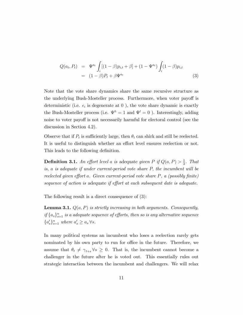
Q(at; Pt) = atZi

[(1� �)pi;t + �] + (1�at)Zi

(1� �)pi;t

= (1� �)Pt + �at (3)

Note that the vote share dynamics share the same recursive structure as

the underlying Bush-Mosteller process. Furthermore, when voter payo¤ is

deterministic (i.e. �i is degenerate at 0 ), the vote share dynamic is exactly

the Bush-Mosteller process (i.e. h = 1 and l = 0 ). Interestingly, adding

noise to voter payo¤ is not necessarily harmful for electoral control (see the

discussion in Section 4.2).

Observe that if Pt is su¢ ciently large, then �t can shirk and still be reelected.

It is useful to distinguish whether an e¤ort level ensures reelection or not.

This leads to the following de�nition.

De�nition 3.1. An e¤ort level a is adequate given P if Q(a; P ) > 12. That

is, a is adequate if under current-period vote share P; the incumbent will be

reelected given e¤ort a. Given current-period vote share P , a (possibly �nite)

sequence of action is adequate if e¤ort at each subsequent date is adequate.

The following result is a direct consequence of (3):

Lemma 3.1. Q(a; P ) is strictly increasing in both arguments. Consequently,if fasgns=1 is a adequate sequence of e¤orts, then so is any alternative sequencefa0sgns=1 where a0s � as 8s.

In many political systems an incumbent who loses a reelection rarely gets

nominated by his own party to run for o¢ ce in the future. Therefore, we

assume that �t 6= t+s 8s � 0. That is, the incumbent cannot become a

challenger in the future after he is voted out. This essentially rules out

strategic interaction between the incumbent and challengers. We will relax

11

this assumption in Section 5.4. We will also assume that if the challenger

wins the election, the propensity for the new incumbent is reset at 12. In

other words, the electorate is neutral towards a new incumbent. This is a

reasonable assumption because in a context of moral hazard, reelection is a

disciplining mechanism rather than a mechanism to select a competent leader

as in an adverse selection context.

Lemma 3.2 below is a simple observation that in the optimum, the incumbent

either exert su¢ cient e¤ort to remain in o¢ ce forever, or shirks and is voted

out.

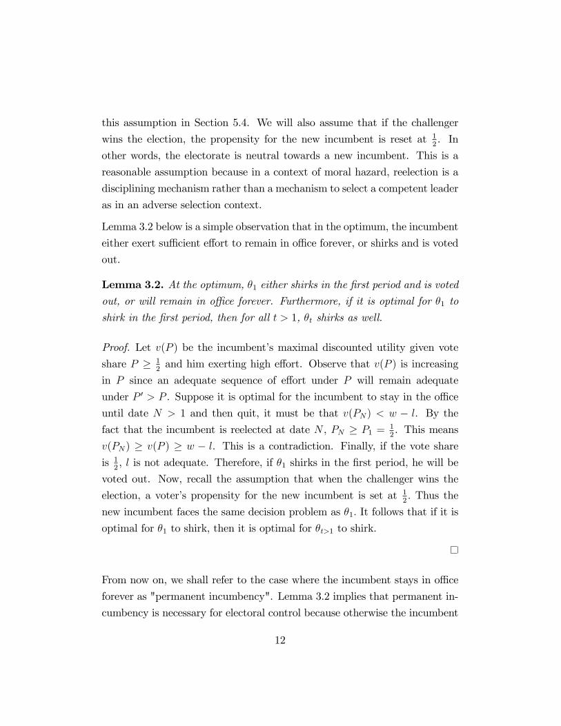
Lemma 3.2. At the optimum, �1 either shirks in the �rst period and is votedout, or will remain in o¢ ce forever. Furthermore, if it is optimal for �1 to

shirk in the �rst period, then for all t > 1, �t shirks as well.

Proof. Let v(P ) be the incumbent�s maximal discounted utility given vote

share P � 12and him exerting high e¤ort. Observe that v(P ) is increasing

in P since an adequate sequence of e¤ort under P will remain adequate

under P 0 > P . Suppose it is optimal for the incumbent to stay in the o¢ ce

until date N > 1 and then quit, it must be that v(PN) < w � l. By thefact that the incumbent is reelected at date N , PN � P1 =

12. This means

v(PN) � v(P ) � w � l. This is a contradiction. Finally, if the vote shareis 1

2, l is not adequate. Therefore, if �1 shirks in the �rst period, he will be

voted out. Now, recall the assumption that when the challenger wins the

election, a voter�s propensity for the new incumbent is set at 12: Thus the

new incumbent faces the same decision problem as �1: It follows that if it is

optimal for �1 to shirk, then it is optimal for �t>1 to shirk.

From now on, we shall refer to the case where the incumbent stays in o¢ ce

forever as "permanent incumbency". Lemma 3.2 implies that permanent in-

cumbency is necessary for electoral control because otherwise the incumbent

12

shirks every period.15 We will henceforth take as given the optimality of per-

manent incumbency unless otherwise stated. Lemma 3.3 below states that

permanent incumbency is optimal if the incumbent is su¢ ciently patient.

Lemma 3.3. Permanent incumbency is optimal if � > 1� w�hw�l .

To properly discuss electoral control, which is typically some measure of

voters�long-run payo¤, we need to characterize the optimal sequence of ef-

forts. Proposition 3.1 is an important step towards this goal. It shows that

the optimal e¤ort at any given period is a function of the vote share at that

period. In particular, the function is a cut-o¤ rule.

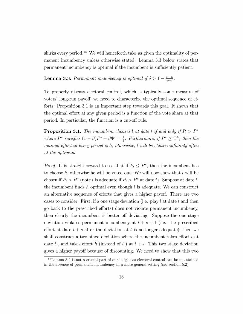
Proposition 3.1. The incumbent chooses l at date t if and only if Pt > P �

where P � satis�es (1� �)P � + �l = 12. Furthermore, if P � � h, then the

optimal e¤ort in every period is h, otherwise, l will be chosen in�nitely often

at the optimum.

Proof. It is straightforward to see that if Pt � P �, then the incumbent hasto choose h, otherwise he will be voted out. We will now show that l will be

chosen if Pt > P � (note l is adequate if Pt > P � at date t). Suppose at date t,

the incumbent �nds h optimal even though l is adequate. We can construct

an alternative sequence of e¤orts that gives a higher payo¤. There are two

cases to consider. First, if a one stage deviation (i.e. play l at date t and then

go back to the prescribed e¤orts) does not violate permanent incumbency,

then clearly the incumbent is better o¤ deviating. Suppose the one stage

deviation violates permanent incumbency at t + s + 1 (i.e. the prescribed

e¤ort at date t + s after the deviation at t is no longer adequate), then we

shall construct a two stage deviation where the incumbent takes e¤ort l at

date t , and takes e¤ort h (instead of l ) at t + s. This two stage deviation

gives a higher payo¤ because of discounting. We need to show that this two

15Lemma 3.2 is not a crucial part of our insight as electoral control can be maintainedin the absence of permanent incumbency in a more general setting (see section 5.2)

13

stage deviation is adequate. The following observations are important for

the proof.

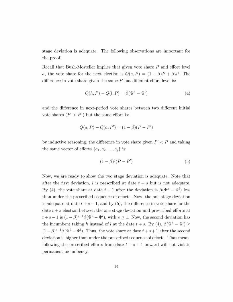
Recall that Bush-Mosteller implies that given vote share P and e¤ort level

a, the vote share for the next election is Q(a; P ) = (1 � �)P + �a: Thedi¤erence in vote share given the same P but di¤erent e¤ort level is:

Q(h; P )�Q(l; P ) = �(h �l) (4)

and the di¤erence in next-period vote shares between two di¤erent initial

vote shares (P 0 < P ) but the same e¤ort is:

Q(a; P )�Q(a; P 0) = (1� �)(P � P 0)

by inductive reasoning, the di¤erence in vote share given P 0 < P and taking

the same vector of e¤orts fa1; a2 : : : ; ajg is:

(1� �)j(P � P 0) (5)

Now, we are ready to show the two stage deviation is adequate. Note that

after the �rst deviation, l is prescribed at date t + s but is not adequate.

By (4), the vote share at date t + 1 after the deviation is �(h � l) lessthan under the prescribed sequence of e¤orts. Now, the one stage deviation

is adequate at date t+ s� 1, and by (5), the di¤erence in vote share for thedate t+ s election between the one stage deviation and prescribed e¤orts at

t+ s� 1 is (1� �)s�1�(h�l), with s � 1. Now, the second deviation hasthe incumbent taking h instead of l at the date t+ s. By (4), �(h �l) �(1��)s�1�(h�l). Thus, the vote share at date t+ s+1 after the seconddeviation is higher than under the prescribed sequence of e¤orts. That means

following the prescribed e¤orts from date t + s + 1 onward will not violate

permanent incumbency.

14

Now, since P1 = 12< h , incumbent�s vote share at any given point cannot

exceed h: Thus if the threshold is larger than h; the incumbent never

shirks. If P � < h, then if incumbent exert high e¤ort for many periods,

the vote share will converge to h and therefore exceed P � at some point. It

follows that the incumbent will shirk in�nitely often at the optimum.

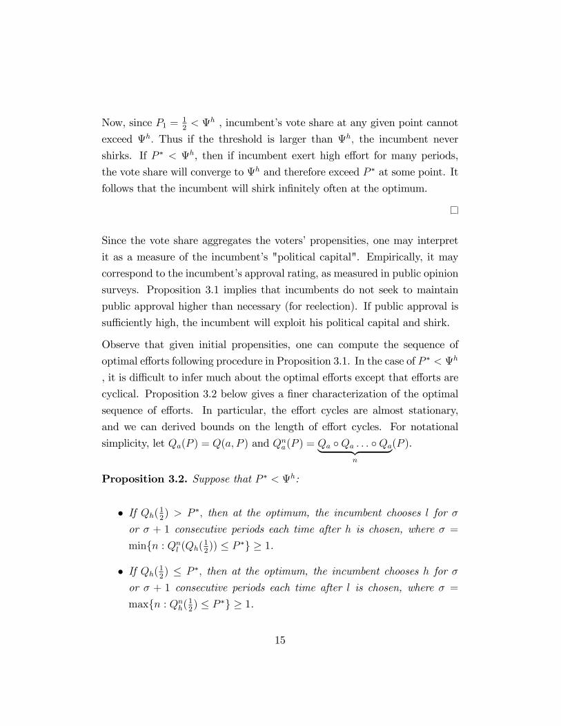
Since the vote share aggregates the voters�propensities, one may interpret

it as a measure of the incumbent�s "political capital". Empirically, it may

correspond to the incumbent�s approval rating, as measured in public opinion

surveys. Proposition 3.1 implies that incumbents do not seek to maintain

public approval higher than necessary (for reelection). If public approval is

su¢ ciently high, the incumbent will exploit his political capital and shirk.

Observe that given initial propensities, one can compute the sequence of

optimal e¤orts following procedure in Proposition 3.1. In the case of P � < h

, it is di¢ cult to infer much about the optimal e¤orts except that e¤orts are

cyclical. Proposition 3.2 below gives a �ner characterization of the optimal

sequence of e¤orts. In particular, the e¤ort cycles are almost stationary,

and we can derived bounds on the length of e¤ort cycles. For notational

simplicity, let Qa(P ) = Q(a; P ) and Qna(P ) = Qa �Qa : : : �Qa| {z }n

(P ).

Proposition 3.2. Suppose that P � < h:

� If Qh(12) > P �; then at the optimum, the incumbent chooses l for �

or � + 1 consecutive periods each time after h is chosen, where � =

minfn : Qnl (Qh(12)) � P�g � 1.

� If Qh(12) � P �; then at the optimum, the incumbent chooses h for �

or � + 1 consecutive periods each time after l is chosen, where � =

maxfn : Qnh(12) � P�g � 1.

15

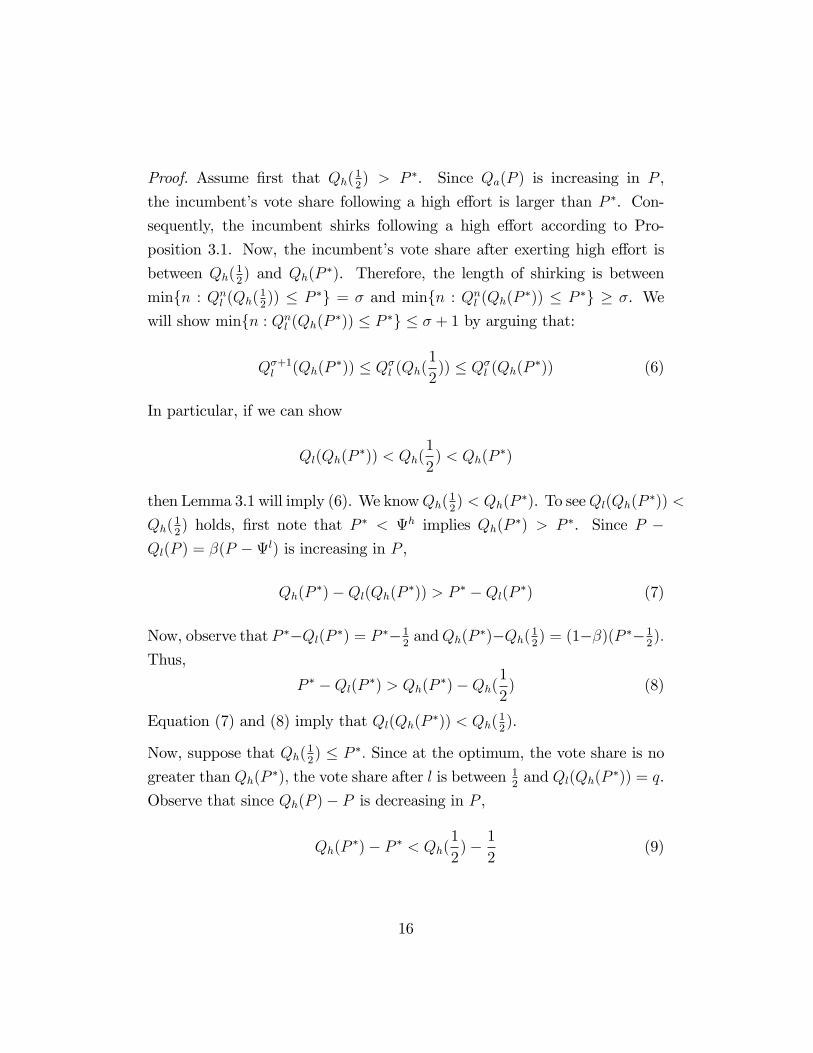
Proof. Assume �rst that Qh(12) > P �. Since Qa(P ) is increasing in P ,

the incumbent�s vote share following a high e¤ort is larger than P �. Con-

sequently, the incumbent shirks following a high e¤ort according to Pro-

position 3.1. Now, the incumbent�s vote share after exerting high e¤ort is

between Qh(12) and Qh(P�). Therefore, the length of shirking is between

minfn : Qnl (Qh(12)) � P �g = � and minfn : Qnl (Qh(P �)) � P �g � �. We

will show minfn : Qnl (Qh(P �)) � P �g � � + 1 by arguing that:

Q�+1l (Qh(P�)) � Q�l (Qh(

1

2)) � Q�l (Qh(P �)) (6)

In particular, if we can show

Ql(Qh(P�)) < Qh(

1

2) < Qh(P

�)

then Lemma 3.1 will imply (6). We knowQh(12) < Qh(P�). To seeQl(Qh(P �)) <

Qh(12) holds, �rst note that P � < h implies Qh(P �) > P �. Since P �

Ql(P ) = �(P �l) is increasing in P ,

Qh(P�)�Ql(Qh(P �)) > P � �Ql(P �) (7)

Now, observe that P ��Ql(P �) = P ��12andQh(P �)�Qh(12) = (1��)(P

��12):

Thus,

P � �Ql(P �) > Qh(P �)�Qh(1

2) (8)

Equation (7) and (8) imply that Ql(Qh(P �)) < Qh(12).

Now, suppose that Qh(12) � P�: Since at the optimum, the vote share is no

greater than Qh(P �); the vote share after l is between 12and Ql(Qh(P �)) = q.

Observe that since Qh(P )� P is decreasing in P ,

Qh(P�)� P � < Qh(

1

2)� 1

2(9)

16

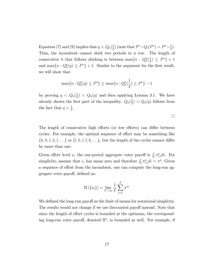
Equation (7) and (9) implies that q < Qh(12) (note that P��Ql(P �) = P ��1

2).

Thus, the incumbent cannot shirk two periods in a row. The length of

consecutive h that follows shirking is between maxfn : Qnh(12) � P �g + 1and maxfn : Qnh(q) � P �g + 1. Similar to the argument for the �rst result,we will show that

maxfn : Qnh(q) � P �g � maxfn : Qnh(1

2) � P �g � 1

by proving q < Qh(12) < Qh(q) and then applying Lemma 3.1. We have

already shown the �rst part of the inequality. Qh(12) < Qh(q) follows from

the fact that q > 12:

The length of consecutive high e¤orts (or low e¤orts) can di¤er between

cycles. For example, the optimal sequence of e¤ort may be something like

fh; h; l; h; l; : : :g or fl; h; l; l; h; : : :g, but the length of the cycles cannot di¤erby more than one.

Given e¤ort level a, the one-period aggregate voter payo¤ isRi�ai;tdi. For

simplicity, assume that �i has mean zero and thereforeRi�ai;tdi = �

a: Given

a sequence of e¤ort from the incumbent, one can compute the long-run ag-

gregate voter payo¤, de�ned as:

�(fatg) = limT!1

1

T

TXt=1

�at

We de�ned the long-run payo¤as the limit of means for notational simplicity.

The results would not change if we use discounted payo¤ instead. Note that

since the length of e¤ort cycles is bounded at the optimum, the correspond-

ing long-run voter payo¤, denoted ��, is bounded as well. For example, if

17

Qh(12) � P �; then

�

� + 1�h +

1

� + 1�l � �� � � + 1

� + 2�h +

1

� + 2�l

A similar bound can be derived for the case of Qh(12) > P�. Note that the

width of the bound is small for large �, and therefore the bounds can be a

good approximation for ��.

We use the lower bound of ��as the measure of electoral control. All of our

comparative statics would follow if we used the upper bound instead.

De�nition 3.2. Let electoral control e be the lower bound of ��; that is:

e =

8<: ��+1�h + 1

�+1�l if Qh(12) � P

�

1�+2�h + �+1

�+2�l if Qh(12) > P

�

where � is de�ned in Proposition 3.2.

Observe that e is maximized (i.e. e = �h) if the incumbent never shirks.

Proposition 3.1 shows that this is the case for some speci�cations of the

parameters. Therefore, electoral control with behavioral voters can be greater

than the electoral control with rational voters as in the Ferejohn model, where

there is always a strictly positive probability that the incumbent shirks.

4 Comparative Statics

In this section, we explore the relationship between various primitives of our

model and electoral control. In particular, we look at novel issues such as

when voter ignorance and forgetfulness can improve electoral control. Note

that since e is a strictly monotonic function of �, we will often treat � as

electoral control to simplify notations in the proofs.

18

4.1 The Value of O¢ ce

One of the fundamental insights provided by the rational voting theory of

electoral control is that a higher value of o¢ ce or lower cost of e¤ort improves

electoral control (Besley and Case 1995, Ferraz and Finan 2008, Ferraz and

Finan 2009, Ferraz and Finan 2011, Alt, de Mesquita, and Rose 2011). These

observations continue to hold in our framework as a corollary to Lemma 3.3.

In particular, high value of o¢ ce and low (relative) cost of high e¤ort helps

sustaining permanent incumbency, which is necessary for electoral control.

Corollary 4.1. If w is su¢ ciently low or h� l su¢ ciently high, e is minimaland equal to �l. For high values of w or low values of h� l, e > �l.

One can see from Proposition 3.1 and Proposition 3.2 that electoral control

given permanent incumbency does not depend on w; h nor l. Thus, w and

h� l a¤ect electoral control only in determining the optimality of permanentincumbency. Finally, if there is a �nite term limit, then the continuation

value of exerting high e¤ort is less than without term limits. It follows that

the incumbent has a higher incentive to shirk, and electoral control su¤ers.16

4.2 Informativeness of E¤orts

A second important �nding of the existing literature pertains to the inform-

ativeness of the signal observed by the electorate: electoral control improves

if observed outcomes become more informative of incumbent�s e¤ort (e.g.

Berry and Howell 2007, Snyder and Strömberg 2010, Ashworth 2012). Re-

call the interpretation of h and l: h is large (l small) if the impact of

noisy events on voter behavior is small vis-a-vis factors within incumbent�s

16For the impact on term-limits see Besley and Case (1995), Ferraz and Finan (2008),Ferraz and Finan (2011), Alt, de Mesquita, and Rose (2011).

19

control. Thus, one may interpret h and l as measures the informativeness

of e¤ort even though our voters are not Bayesians.

Unlike in standard models, the e¤ect of informativeness of high and low e¤ort

on electoral control is asymmetric. In particular, electoral control improves

when the electorate is in�uenced by factors that are informative of low e¤ort

but uninformative of high e¤ort. This is intuitive because if the electorate

is particularly sensitive to high e¤ort, then it is easier for the politicians

to build up political capital, which allows the politicians to shirk; while if

the electorate is sensitive to low e¤ort, then shirking is very costly for the

politicians. Thus, to improve electoral control voters should be skeptical, but

unforgiving. This is stated formally in the following proposition.

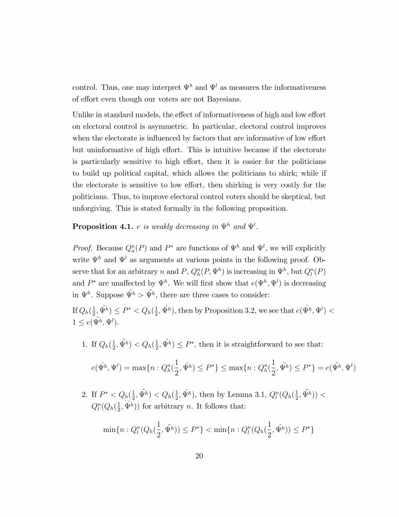
Proposition 4.1. e is weakly decreasing in h and l:

Proof. Because Qna(P ) and P� are functions of h and l, we will explicitly

write h and l as arguments at various points in the following proof. Ob-

serve that for an arbitrary n and P , Qnh(P;h) is increasing in h, but Qnl (P )

and P � are una¤ected by h. We will �rst show that e(h;l) is decreasing

in h. Suppose ̂h > ~h, there are three cases to consider:

IfQh(12 ;~h) � P � < Qh(12 ; ̂h); then by Proposition 3.2, we see that e(̂h;

l) <

1 � e( ~h;l).

1. If Qh(12 ;~h) < Qh(

12; ̂h) � P �; then it is straightforward to see that:

e(̂h;l) = maxfn : Qnh(1

2; ̂h) � P �g � maxfn : Qnh(

1

2; ~h) � P �g = e( ~h;l)

2. If P � < Qh(12 ;~h) < Qh(

12; ̂h), then by Lemma 3.1, Qnl (Qh(

12; ~h)) <

Qnl (Qh(12; ̂h)) for arbitrary n. It follows that:

minfn : Qnl (Qh(1

2; ~h)) � P �g < minfn : Qnl (Qh(

1

2; ̂h)) � P �g

20

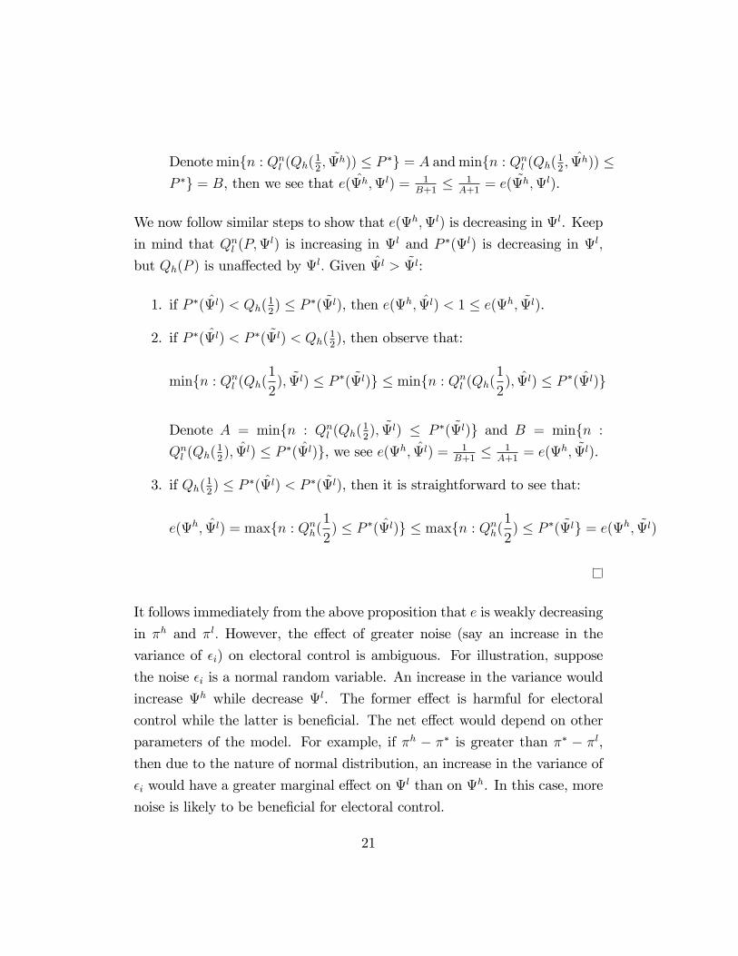
Denoteminfn : Qnl (Qh(12 ; ~h)) � P�g = A andminfn : Qnl (Qh(12 ; ̂h)) �

P �g = B, then we see that e(̂h;l) = 1B+1

� 1A+1

= e( ~h;l).

We now follow similar steps to show that e(h;l) is decreasing in l. Keep

in mind that Qnl (P;l) is increasing in l and P �(l) is decreasing in l;

but Qh(P ) is una¤ected by l: Given ̂l > ~l:

1. if P �(̂l) < Qh(12) � P�( ~l), then e(h; ̂l) < 1 � e(h; ~l).

2. if P �(̂l) < P �( ~l) < Qh(12), then observe that:

minfn : Qnl (Qh(1

2); ~l) � P �( ~l)g � minfn : Qnl (Qh(

1

2); ̂l) � P �(̂l)g

Denote A = minfn : Qnl (Qh(12); ~l) � P �( ~l)g and B = minfn :Qnl (Qh(

12); ̂l) � P �(̂l)g, we see e(h; ̂l) = 1

B+1� 1

A+1= e(h; ~l).

3. if Qh(12) � P�(̂l) < P �( ~l), then it is straightforward to see that:

e(h; ̂l) = maxfn : Qnh(1

2) � P �(̂l)g � maxfn : Qnh(

1

2) � P �( ~lg = e(h; ~l)

It follows immediately from the above proposition that e is weakly decreasing

in �h and �l: However, the e¤ect of greater noise (say an increase in the

variance of �i) on electoral control is ambiguous. For illustration, suppose

the noise �i is a normal random variable. An increase in the variance would

increase h while decrease l. The former e¤ect is harmful for electoral

control while the latter is bene�cial. The net e¤ect would depend on other

parameters of the model. For example, if �h � �� is greater than �� � �l,then due to the nature of normal distribution, an increase in the variance of

�i would have a greater marginal e¤ect on l than on h. In this case, more

noise is likely to be bene�cial for electoral control.

21

4.3 Voter Memory

In this section, we explore a new dimension of electoral control: the connec-

tion between voter memory and electoral control. Recall our interpretation

of � as a measure of voter�s forgetfulness: a higher � means the date t ex-

perience has a greater weight on determining the date t + 1 propensity. In

the extreme case of satis�cing (� = 1), the date t + 1 propensity is solely

determined by the date t experience.

The following result indicates that a high level of electoral control is obtained

when the voters are su¢ ciently forgetful. Intuitively, for a high level of

forgetfulness, the incumbent�s action at date t has a large impact on the

outcome of election at t + 1, but its impact on the outcome of election at

t+2, t+3; : : : is small (since the outcome in those elections is a¤ected mostly

by actions in t+1; t+2; : : :). Consequently, the degree of voter forgetfulness

determines how myopic or farsighted the incumbent is when choosing e¤ort.

And since for su¢ ciently large �, high e¤ort is needed for reelection, a myopic

incumbent would have very high incentive to exert high e¤ort. It follows that

electoral control is maximized in this case.

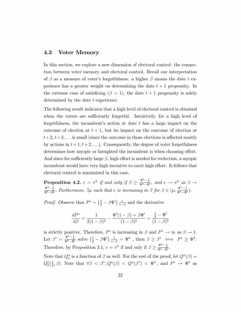
Proposition 4.2. e = �h if and only if � � h� 12

h�l , and e ! �h as � !h� 1

2

h�l : Furthermore, 9� such that e is increasing in � for � 2 (�;h� 1

2

h�l ):

Proof. Observe that P � =�12� �l

�11�� and the derivative

dP �

d�=

1

2(1� �)2 �l(1� �) + �l

(1� �)2 =12�l

(1� �)2

is strictly positive. Therefore, P � is increasing in � and P � !1 as � ! 1.

Let �� = h� 12

h�l solve�12� �l

�11�� = h , then � � �� () P � � h.

Therefore, by Proposition 3.1, e = �h if and only if � � h� 12

h�l .

Note that Qna is a function of � as well. For the rest of the proof, let Qn(�) =

Qnh(12; �): Note that 8� < ��; Qn(�) < Qn(��) < h , and P � ! h as

22

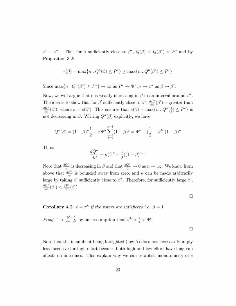
� ! �� . Thus for � su¢ ciently close to ��, Q(�) < Q(��) < P � and by

Proposition 3.2:

e(�) = maxfn : Qn(�) � P �g � maxfn : Qn(��) � P �g

Since maxfn : Qn(��) � P �g ! 1 as P � ! h, e! �h as � ! ��.

Now, we will argue that e is weakly increasing in � in an interval around ��.

The idea is to show that for �0 su¢ ciently close to ��, dP�

d�(�0) is greater than

dQ�

d�(�0), where � = e(�0). This ensures that e(�) = maxfn : Qn(1

2) � P �g is

not decreasing in �. Writing Qn(�) explicitly, we have

Qn(�) = (1� �)n12+ �h

n�1Xj=0

(1� �)j = h + (12�h)(1� �)n

Thus:dQn

d�= n(h � 1

2)(1� �)n�1

Note that dQn

d�is decreasing in � and that dQ

n

d�! 0 as n!1. We know from

above that dP �

d�is bounded away from zero, and � can be made arbitrarily

large by taking �0 su¢ ciently close to ��. Therefore, for su¢ ciently large �0,dQ�

d�(�0) < dP �

d�(�0).

Corollary 4.2. e = �h if the voters are satis�cers i.e. � = 1

Proof. 1 > h� 12

h�l by our assumption that h > 1

2> l.

Note that the incumbent being farsighted (low �) does not necessarily imply

less incentive for high e¤ort because both high and low e¤ort have long run

a¤ects on outcomes. This explain why we can establish monotonicity of e

23

with respect to � for high levels of �. In sum, we have shown that highly

forgetful voters as identi�ed by Achen and Bartels (2004a) can induce high

levels of electoral control, but, as we will show in Section 5.3, this conclusion

does depend on the frequency of elections. Recall that highly forgetful voters

induce the incumbent to behave myopically. This is bene�cial for electoral

control when elections are frequent (i.e. held in every period). However, when

elections are held once every k > 1 periods, a myopic incumbent would have

little incentive to exert high e¤ort except in periods close to an election. This

suggests that highly forgetful voters is likely to be bad for electoral control

when elections are infrequent.

5 Generalizations

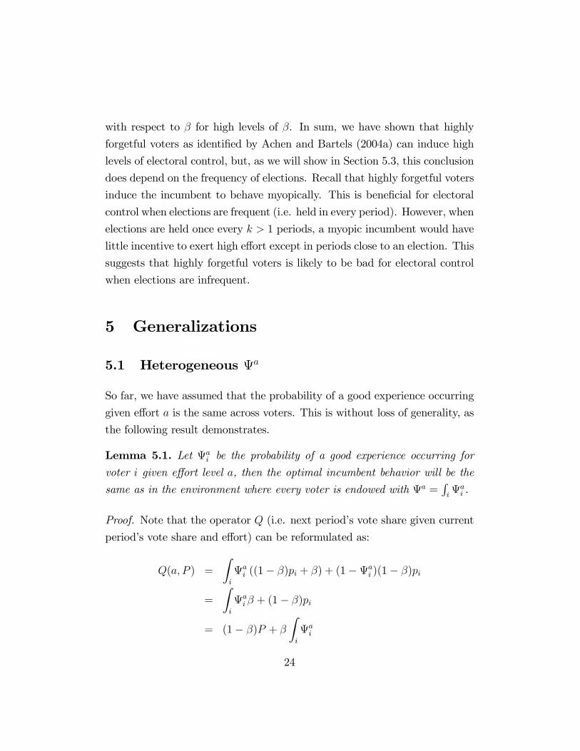
5.1 Heterogeneous a

So far, we have assumed that the probability of a good experience occurring

given e¤ort a is the same across voters. This is without loss of generality, as

the following result demonstrates.

Lemma 5.1. Let ai be the probability of a good experience occurring forvoter i given e¤ort level a, then the optimal incumbent behavior will be the

same as in the environment where every voter is endowed with a =Riai .

Proof. Note that the operator Q (i.e. next period�s vote share given current

period�s vote share and e¤ort) can be reformulated as:

Q(a; P ) =

Zi

ai ((1� �)pi + �) + (1�ai )(1� �)pi

=

Zi

ai � + (1� �)pi

= (1� �)P + �Zi

ai

24

Since the operator Q is the only relevant information for the incumbent�s

problem, we see that electoral control in an environment with heterogeneous

ai is equivalent to an environment with homogenous voters.

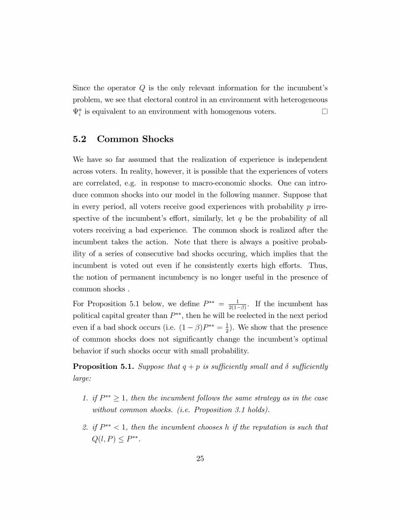
5.2 Common Shocks

We have so far assumed that the realization of experience is independent

across voters. In reality, however, it is possible that the experiences of voters

are correlated, e.g. in response to macro-economic shocks. One can intro-

duce common shocks into our model in the following manner. Suppose that

in every period, all voters receive good experiences with probability p irre-

spective of the incumbent�s e¤ort, similarly, let q be the probability of all

voters receiving a bad experience. The common shock is realized after the

incumbent takes the action. Note that there is always a positive probab-

ility of a series of consecutive bad shocks occuring, which implies that the

incumbent is voted out even if he consistently exerts high e¤orts. Thus,

the notion of permanent incumbency is no longer useful in the presence of

common shocks .

For Proposition 5.1 below, we de�ne P �� = 12(1��) . If the incumbent has

political capital greater than P ��, then he will be reelected in the next period

even if a bad shock occurs (i.e. (1� �)P �� = 12). We show that the presence

of common shocks does not signi�cantly change the incumbent�s optimal

behavior if such shocks occur with small probability.

Proposition 5.1. Suppose that q + p is su¢ ciently small and � su¢ cientlylarge:

1. if P �� � 1, then the incumbent follows the same strategy as in the casewithout common shocks. (i.e. Proposition 3.1 holds).

2. if P �� < 1, then the incumbent chooses h if the reputation is such that

Q(l; P ) � P ��.

25

Proof. For the �rst result, note that if P �� � 1, then the incumbent will bekicked out with probability q each period regardless of his e¤orts. Let P �be

as de�ned in Proposition 3.1. If P � P �, then the di¤erence in probabilityof reelection between high e¤ort and low e¤ort is 1 � p � q. Let v be thecontinuation value given high e¤ort, the incumbent should choose high e¤ort

if � � (1� p� q) � v is greater than h� l. This is true if � is large and q small,since v would be large in that case. Finally, it is straightforward to see that

if P > P �; then the two stage deviation argument applies, and therefore l is

optimal if P > P �:

For the second result, we have to argue that a su¢ ciently patient incumbent

has a strict incentive to maintain his reputation above P ��. In particular,

we want to show that the bene�t of exerting high e¤ort when P is below

P �� (i.e. an greater of probability of being reelected in the future) outweighs

the loss of utility due to high e¤ort. Let vP be the optimal discounted

utility given reputation level P (note that vP is increasing in P ). Suppose

P is such that Q(l; P ) � P �� < Q(h; P ); then if the incumbent chooses h,

he will have a higher probability of being reelected two periods from now

than if he were to choose l (since the vote share next period will be above

P ��). Let this di¤erence in probability be 4, then he should choose h if� � 4 � vP 0 > h� l where P 0 is the next period�s vote share given high e¤ort(and no shocks occurring). Now, since w � h > 0, vP ! 1 as � ! 1

and p + q ! 0. Therefore for su¢ ciently large � and small probability of

common shocks, high e¤ort will be optimal. Now suppose P < P �� is such

that Q(h; P ) = Qh(P ) < P �� < Q2h(P ); if the incumbent exert high e¤ort,

then given the step above, he will exert high e¤ort again next period and his

reputation will be above P �� after two periods (given no shocks occurring).

Therefore, the incumbent�s probability of being reelected three periods into

the future will be higher if he exert high e¤ort now rather than low e¤ort.

Again, for su¢ ciently patient incumbent and low probability of common

shock, this di¤erence in probability is enough to induce high e¤ort now. We

26

can iterate the same argument for P where Qn�1h (P ) < P �� < Qnh(P ) for any

n.

The second result in Proposition 5.1 suggests that the presence of common

shocks can improve electoral control. This follows from the fact that in the

baseline model, high e¤ort is exerted if and only if Q(l; P ) � 12, while here

the threhold for high e¤ort is P ��, which may be greater than 12. Intuitively,

the incumbent wishes to insulate himself against a bad shock by maintain-

ing higher political capital than in an environment without common shocks.

Thus, he needs to exert high e¤ort more often.

5.3 Multi-period Incumbency

In this section, we examine the incumbent�s behavior when an election is

held every k > 1 periods. That is, there is an election at date 1, k+1, 2k+1

and so on. Note that k = 1 corresponds to the baseline model in Section 2.

We show that the optimal e¤ort is still determined by a threshold rule even

though the incumbent no longer needs to maintain a vote share of 12in every

period. This rule is stationary in the sense that threshold rule for date t will

be the same as that for date t + k. To simplify notations, we will refer to

dates t 2 f� ; k + 1 � � ; 2k + 1 � � ; : : :g collectively as � . That is, � � k is

the number of period until the next election (e.g. � = 1 denotes dates prior

to an election, and � = k denotes election dates. )

Proposition 5.2. At date � ; the incumbent maintains P� > P ��� and he

shirks if and only if P� > P �� . where P��� and P �� are de�ned as follows:

If � < 1,

27

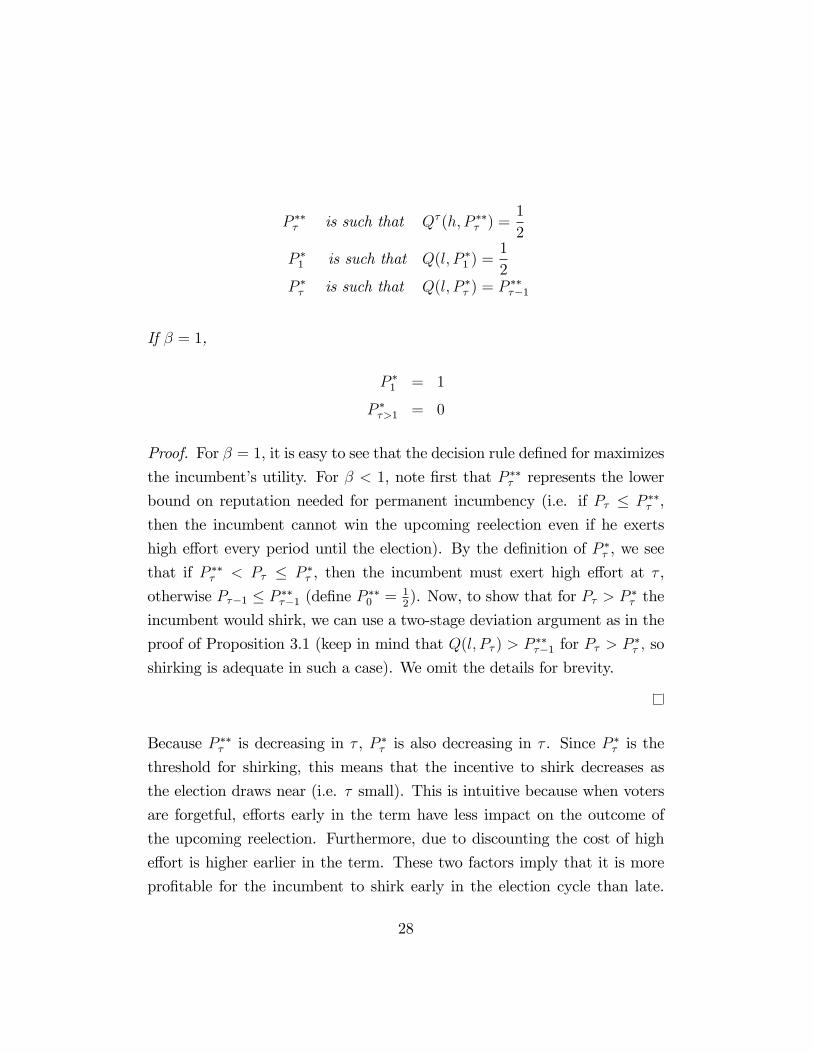
P ��� is such that Q� (h; P ��� ) =1

2

P �1 is such that Q(l; P �1 ) =1

2P �� is such that Q(l; P �� ) = P

����1

If � = 1,

P �1 = 1

P ��>1 = 0

Proof. For � = 1, it is easy to see that the decision rule de�ned for maximizes

the incumbent�s utility. For � < 1, note �rst that P ��� represents the lower

bound on reputation needed for permanent incumbency (i.e. if P� � P ��� ,

then the incumbent cannot win the upcoming reelection even if he exerts

high e¤ort every period until the election). By the de�nition of P �� , we see

that if P ��� < P� � P �� , then the incumbent must exert high e¤ort at � ,

otherwise P��1 � P ����1 (de�ne P ��0 = 12). Now, to show that for P� > P �� the

incumbent would shirk, we can use a two-stage deviation argument as in the

proof of Proposition 3.1 (keep in mind that Q(l; P� ) > P ����1 for P� > P�� ; so

shirking is adequate in such a case). We omit the details for brevity.

Because P ��� is decreasing in � , P �� is also decreasing in � . Since P�� is the

threshold for shirking, this means that the incentive to shirk decreases as

the election draws near (i.e. � small). This is intuitive because when voters

are forgetful, e¤orts early in the term have less impact on the outcome of

the upcoming reelection. Furthermore, due to discounting the cost of high

e¤ort is higher earlier in the term. These two factors imply that it is more

pro�table for the incumbent to shirk early in the election cycle than late.

28

Corollary 5.1 formalizes this intuition by showing that in the optimum, the

incumbent shirks prior to some point in the election cycle and exerts high

e¤ort thereafter.

We also provide a bound on the proportion of high e¤orts to low e¤orts within

an election cycle, and this bound is independent of k and decreasing in �: One

implication of the result is that ceteris paribus, high frequency of elections is

good for electoral control. A second implication is that when elections are

infrequent, highly forgetful voters are no longer a boon for electoral control.

For example, when voters are satis�cers i.e. � = 1, electoral control is

minimized if k > 1 while maximized if k = 1.

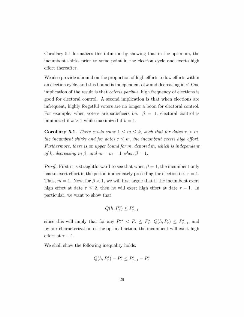
Corollary 5.1. There exists some 1 � m � k; such that for dates � > m;

the incumbent shirks and for dates � � m, the incumbent exerts high e¤ort.Furthermore, there is an upper bound for m; denoted �m, which is independent

of k, decreasing in �, and �m = m = 1 when � = 1.

Proof. First it is straightforward to see that when � = 1, the incumbent only

has to exert e¤ort in the period immediately preceding the election i.e. � = 1.

Thus, m = 1. Now, for � < 1, we will �rst argue that if the incumbent exert

high e¤ort at date � � 2, then he will exert high e¤ort at date � � 1. Inparticular, we want to show that

Q(h; P �� ) � P ���1

since this will imply that for any P ��� < P� � P �� , Q(h; P� ) � P ���1, and

by our characterization of the optimal action, the incumbent will exert high

e¤ort at � � 1.

We shall show the following inequality holds:

Q(h; P �� )� P �� � P ���1 � P ��

29

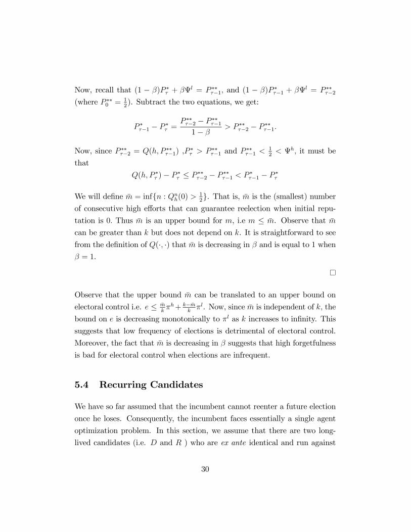
Now, recall that (1 � �)P �� + �l = P ����1; and (1 � �)P ���1 + �l = P ����2

(where P ��0 = 12). Subtract the two equations, we get:

P ���1 � P �� =P ����2 � P ����11� � > P ����2 � P ����1:

Now, since P ����2 = Q(h; P ����1) ,P�� > P ����1 and P

����1 <

12< h; it must be

that

Q(h; P �� )� P �� � P ����2 � P ����1 < P ���1 � P ��

We will de�ne �m = inffn : Qnh(0) > 12g. That is, �m is the (smallest) number

of consecutive high e¤orts that can guarantee reelection when initial repu-

tation is 0: Thus �m is an upper bound for m, i.e m � �m. Observe that �m

can be greater than k but does not depend on k. It is straightforward to see

from the de�nition of Q(�; �) that �m is decreasing in � and is equal to 1 when

� = 1.

Observe that the upper bound �m can be translated to an upper bound on

electoral control i.e. e � �mk�h+ k� �m

k�l. Now, since �m is independent of k; the

bound on e is decreasing monotonically to �l as k increases to in�nity. This

suggests that low frequency of elections is detrimental of electoral control.

Moreover, the fact that �m is decreasing in � suggests that high forgetfulness

is bad for electoral control when elections are infrequent.

5.4 Recurring Candidates

We have so far assumed that the incumbent cannot reenter a future election

once he loses. Consequently, the incumbent faces essentially a single agent

optimization problem. In this section, we assume that there are two long-

lived candidates (i.e. D and R ) who are ex ante identical and run against

30

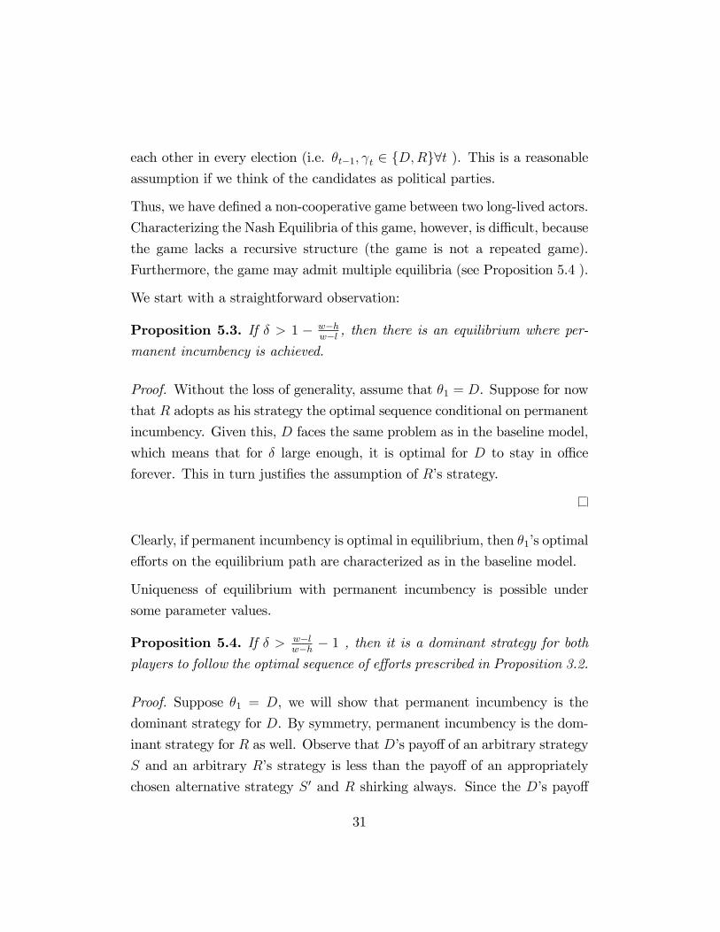
each other in every election (i.e. �t�1; t 2 fD;Rg8t ). This is a reasonableassumption if we think of the candidates as political parties.

Thus, we have de�ned a non-cooperative game between two long-lived actors.

Characterizing the Nash Equilibria of this game, however, is di¢ cult, because

the game lacks a recursive structure (the game is not a repeated game).

Furthermore, the game may admit multiple equilibria (see Proposition 5.4 ).

We start with a straightforward observation:

Proposition 5.3. If � > 1 � w�hw�l , then there is an equilibrium where per-

manent incumbency is achieved.

Proof. Without the loss of generality, assume that �1 = D. Suppose for now

that R adopts as his strategy the optimal sequence conditional on permanent

incumbency. Given this, D faces the same problem as in the baseline model,

which means that for � large enough, it is optimal for D to stay in o¢ ce

forever. This in turn justi�es the assumption of R�s strategy.

Clearly, if permanent incumbency is optimal in equilibrium, then �1�s optimal

e¤orts on the equilibrium path are characterized as in the baseline model.

Uniqueness of equilibrium with permanent incumbency is possible under

some parameter values.

Proposition 5.4. If � > w�lw�h � 1 , then it is a dominant strategy for both

players to follow the optimal sequence of e¤orts prescribed in Proposition 3.2.

Proof. Suppose �1 = D, we will show that permanent incumbency is the

dominant strategy for D. By symmetry, permanent incumbency is the dom-

inant strategy for R as well. Observe that D�s payo¤ of an arbitrary strategy

S and an arbitrary R�s strategy is less than the payo¤ of an appropriately

chosen alternative strategy S 0 and R shirking always. Since the D�s payo¤

31

under permanent incumbency is independent of R�s strategy, showing that

permanent incumbency dominates all other strategies when R always shirks

is su¢ cient to prove the dominance of permanent incumbency.

First, we will show that D�s best response to R shirking always is either

permanent incumbency or shirking always. The argument for this is similar

to the proof of Lemma 3.2. Let vP be D�s maximal discounted payo¤ given

initial distribution P and choosing h. Let ~v be the D�s maximal discounted

payo¤ for choosing l and losing the reelection. Note that ~v does not depend

on the initial distribution of propensities because the propensities for a newly

elected incumbent is reset to 12. Suppose theD�s best response is staying until

period N > 1 and then quit, it must be that vPN < ~v. However, the fact that

PN > P1 and D chose h at date 1 means vPN � vP1 > ~v: A contradiction.

Observe that if it is optimal for D to shirk at date 1, then it must be optimal

to shirk whenever D is elected to o¢ ce. Thus, D�s best response to R�s

strategy involves either permanent incumbency or shirking always. The pay-

o¤ associated with permanent incumbency is at least w�h1�� , while the payo¤

associated with shirking always is w�l1��2 : Therefore, if

w�h1�� >

w�l1��2 () � >

w�lw�h � 1 , then permanent incumbency is the dominant strategy.

Observe that the condition on � in Proposition 5.4 is not the same in the

condition in Proposition 5.3. In particular, the condition in Proposition 5.3

can always be satis�ed by taking � su¢ ciently large, the same cannot be

said for Proposition 5.4 since w�lw�h is not bounded above. The following is a

corollary of Proposition 5.3 and Proposition 5.4.

Corollary 5.2. If � � h� 12

h�l , and � �w�lw�h � 1, then there is an equilibrium

where both D and R always shirk. If, in addition, 1� w�hw�l < �, then there is

also a permanent incumbency equilibrium.

32

Proof. If � � h� 12

h�l , then l is never adequate. That means the payo¤ under

permanent incumbency is exactly w�h1�� : It follows from the proof of Proposi-

tion 5.4 that if w�h1�� �

w�l1��2 () � � w�l

w�h � 1, then D�s best response to Rshirking always is to shirk always. This in turn justi�es R shirking always.

Note that � � h� 12

h�l is a su¢ cient and necessary condition for maximal elect-

oral control in the baseline model. Thus, Corollary 5.2 shows that in some

instances, there can be two extremal equilibria: one in which the incumbent

exercises high e¤orts in every period, and one in which the incumbent shirks

in every period. This multiplicity of equilibria makes it di¢ cult to conduct

comparative statics.17 However, it is straightforward to see that the incum-

bent�s payo¤ under permanent incumbency must be the lower bound of the

equilibrium payo¤, since the incumbent can always deviate to permanent in-

cumbency. The fact that the incumbent�s equilibrium payo¤ is higher than

under permanent incumbency suggests that there is (weakly) more shirk-

ing in equilibrium than under permanent incumbency.18 This can be seen as

evidence that allowing the incumbent to reenter the race after losing is harm-

ful for electoral control. This is in accordance with a corresponding result in

Ferejohn (1986), where electoral control is decreasing in the probability that

an incumbent returns to a race after losing o¢ ce.

17One problem is that for some equilibria, the measure of electoral control de�ned earlier(i.e. e) may not apply since the sequence of e¤orts on an equilibrium path may not bewell-behaved.18Note that the incumbent obtains w in every period under permanent incumbency.

Thus if in a given equilibrium both players were to obtain higher payo¤s, that must meanl is chosen more often.

33

6 Conclusion

Critics of democracy have frequently argued that democratic forms of gov-

ernance require a well-informed and rational electorate (e.g. Dahl 1989). If

voters are found to lack these qualities, so the argument continues, a proper

justi�cation for democracy is lacking (e.g. Achen and Bartels 2004b). In

political economy, much of the debate has centered on whether in reality,

voter behavior is consistent with the rational choice foundation (e.g. Ash-

worth 2012) or not (e.g. Achen and Bartels 2004a) . In this paper, we set

this debate aside and investigate the underlying premise of the controversy:

electoral control of public o¢ cials requires a well-informed and rational elect-

orate. To do so we assume that voters act as the behavioralist critics of the

rational choice models have argued: they are forgetful, uninformed, biased

and care little about politics and policy.

Our model can account for many identi�ed empirical regularities such as the

detrimental e¤ect of lowering o¢ ce bene�ts, e.g. by imposing term limits. We

can also investigate the importance of new factors such as voter forgetfulness.

Surprisingly, if elections are frequently held, electoral control is highest if

voters are most forgetful and ignore all but the most immediate past.

Our results suggest that the institution of electoral control of public o¢ cials

may be far less dependent on the reasoning ability of the electorate than

previously believed. Indeed, behavioral voters may achieve higher levels of

electoral control than rational voters if elections occur frequently. This con-

clusion may no longer hold, however, for less frequent elections.

We also explore variois extensions and variations of the model, such as het-

erogeneity, common shocks, recurring candidates and multi-period incum-

bency. Most extensions con�rm the main results of the paper. Novel issues,

however, are raised by multi-period incumbency, which poses new questions

about the interplay of attention, term length, and voter memory. Potential

extensions include candidate quality as in adverse selection models or issues

34

of policy choice and ideological candidates. Such questions, we hope, will be

the subject of future research.

35

References

[1] Achen, C. & Bartels, L. (2004a). �Blind Retrospection: Electoral Re-

sponses to Drought, Flu, and Shark Attacks.âeï¿12Unpublished manu-

script. Princeton University.

[2] Achen, C., & Bartels, L., (2004b) �Musical Chairs: Pocketbook Voting

and the Limits of Democratic Accountability.�Unpublished manuscript.

Princeton University.

[3] Achen, C., & Bartels, L., (2002) �Ignorance and Bliss in Democratic

Politics: Party Competition with Uninformed Voters.�Unpublished ma-

nuscript. Princeton University.

[4] Alt, J., Bueno de Mesquita E., & Rose S. (2011) �Disentangling Ac-

countability and Competence in Elections: Evidence from US Term

Limits.âeï¿12Journal of Politics 73(1): 171-86.

[5] Andonie, C & Diermeier, D. (2012). �A Behavioral Model of Multi-

Candidate Elections�. working paper.

[6] Ashworth, S. (2012). �Electoral Accountability: Recent Theoretical and

Empirical Work�. Annual Review of Political Science 15:183-201

[7] Ashworth, S. (2005). �Reputational Dynamics and Political

Careersâeï¿12Journal of Law Economics and Organization 21:441-66

[8] Ashworth, S., and Ethan Bueno de Mesquita. (2008). �Electoral Selec-

tion, Strategic Challenger Entry, and the Incumbency Advantage.âeï¿12

Journal of Politics 70 (4): 1006�25.

[9] Ashworth, S., and de Mesquita. (2013a). "Disasters and Incumbent

Electoral Fortunes: No Implications for Democratic Competence."

Mimeo. University of Chicago

36

[10] Ashworth, S., and de Mesquita. (2013b). "Is Voter Competence Good

for Voters?: Information, Rationality, and Democratic Performance."

Mimeo. University of Chicago

[11] Ashworth, S., de Mesquita, E., & Friedenberg, A. (2012). �Accountab-

ility Trapsâeï¿12. mimeo. University of Chicago.

[12] Bailenson, J., Iyengar, S., Yee, N., & Collins, N. (2009). �Facial Sim-

ilarity between Candidates and Voters Causes In�uence.âeï¿12Public

Opinion Quarterly 72: 935-61.

[13] Barro, R. (1973). �The Control of Politicians: An Economic

Model.âeï¿12Public Choice 14 (1): 19�42

[14] Bartels, L.M., (2008). Unequal Democracy. Princeton: Princeton Uni-

versity Press.

[15] Bartels, L. M., & Zaller, J. (2001) �Presidential Vote Models: A

Recount.âeï¿12PS: Political Science and Politics 34: 9-20.

[16] Bellew, C. C., II. & Todorov, A. (2007) �Predicting Political Elections

from Rapid and Unre�ective Face Judgments,âeï¿12Proceedings of the

National Academy of Sciences 104: 17948-53.

[17] Bendor, J., Kumar, S.,&Siegel,D. (2010). �Adaptively Rational Retro-

spective Voting�. Journal of Theoretical Politics, 22: 26-63

[18] Bendor, J. Diermeier, D., Siegel, D., & Ting, M. (2011). �A Behavioral

Theory of Elections�Princeton University Press

[19] Bendor, J., Diermeier, D.,& Ting, M. (2003). �A Behavioral Model of

Turnout�. American Political Science Review, 97(2).

[20] Berelson, B.R., Lazarsfeld, P.F., & McPhee, W.N. (1954). Voting: A

Study of Opinion Formation in a Presidential Campaign. Chicago: Uni-

versity of Chicago Press.

37

[21] Berry, C. R., & Howell, W. G. (2007) �Accountability and Local Elec-

tions: Rethinking Retrospective Voting.âeï¿12Journal of Politics 69(3):

844-58.

[22] Besley, T. & Case, A. (1995) �Does Electoral Accountability Af-

fect Economic Policy Choices? Evidence from Gubernatiorial Term

Limits.âeï¿12Quarterly Journal of Economics. 110(3): 769-98.

[23] Bisin, A., Lizzeri, A., & Yariv, L., (2011) �Government Policy with Time

Inconsistent Voters.âeï¿12Working paper.

[24] Board, S., and Moritz Meyer-Ter-Vehn. (2013). �Reputation for

Quality.âeï¿12Econometrica 81 (6): 2381-2462.

[25] Borgers, T., Sarin, R. (2000). �Naive Reinforcement Learning with En-

dogenous Aspirations�. International Economic Review, 41: 921-950.

[26] Bush, R., Mosteller, F. �Stochastic Models of Learning,�Wiley, New

York, 1955.

[27] Campbell, A., Converse, P., Miller, W., & Stokes, D. (1960). The Amer-

ican Voter. New York: John Wiley & Sons.

[28] Cole, S., Healy, A., & Werker, E. (2012). �Do Voters Demand Respons-

ive Governments? Evidence from Indian Disaster Relief." Journal of

Development Economics 97: 167-181.

[29] Dahl, R. A. (1989). Democracy and Its Critics. New Haven: Yale Uni-

versity Press.

[30] Duch, R. M., & Stevenson, R. D. (2008) The Economic Vote. New York:

Cambridge University Press.

[31] Erikson, R. S. (1990) �Economic Conditions and the Congressional

Vote: A Review of the Macro-Level Evidence.âeï¿12American Journal

of Political Science 34: 373-99.

38

[32] Erikson, R.S. (1989). �Economic Conditions and the Presidential

Vote.âeï¿12American Political Science Review 83: 568 -73.

[33] Fair, R. (1978). �The E¤ect of Economic Events on Votes for

President.âeï¿12Review of Economics and Statistics 60: 159-72.

[34] Fearon, J. (1999). �Electoral Accountability and the Control of

Politicians.âeï¿12In Democracy, Accountability and Representation, eds.

Adam Przeworski, Susan C. Stokes, and Bernard Manin. New York:

Cambridge University Press, 55�97

[35] Ferejohn, J. (1986). �Incumbent Performance and Electoral Control�.

Public Choice 50:5-25

[36] Ferraz, C., & Finan, F. (2011) �Electoral Accountability and Corrup-

tion: Evidence from the Audits of Local Governments.âeï¿12American

Economic Review 101(4): 1274-311.

[37] Ferraz, C., & Finan, F. (2009) �Motivating Politicians: The Impacts of

Monetary Incentives on Quality and Performance.âeï¿12Working Paper.

[38] Ferraz, C., & Finan, F. (2008) �Exposing Corrupt Politicians: The Ef-

fect of Brazil�s Publicly Released Audits on Electoral Outcomes.âeï¿12

Quarterly Journal of Economics 123(2): 703-45.

[39] Gasper, J.T. & Reeves, A. (2011). �Make it Rain? Retrospection and

the Attentive Electorate in the Context of Natural Disasters." American

Journal of Political Science 55(2): 340-355.

[40] Harrington Jr, J. (1993) �Economic Policy, Economic Performance and

Elections�American Economic Review 83:27-42

[41] Healy, A., Mo, C., & Malhotra, N. (2010). �Irrelevant Events A¤ect

Voters�Evaluations of Government Performance.âeï¿12Proceedings of

the National Academy of Sciences 107(28): 12506-12511.

39

[42] Healy A, and Gabriel S. Lenz (2014) �Substituting the End for the

Whole: Why Voters Respond Primarily to the Election-Year Economy�

American Journal of Political Science 58 (1):31-47

[43] Hibbs, D. A. Jr. (2006). �Voting and the Macroeconomy.âeï¿12In Wein-

gast, B. R. and Wittmen, D., eds., The Oxford Handbook of Political

Economy, 565-586. Oxford: Oxford University Press.

[44] Hilgard, E.R. & Bower, G.H. (1966). Theories of Learning. New York:

Appleton-Century-Crofts.

[45] Huber, G.A., Hill, S.J., Lenz, G. S. (2012) �Sources of Bias in Retro-

spective Decision Making: Experimental Evidence on Voters�Limita-

tions in Controlling Incumbents.âeï¿12American Political Science Re-

view 106(4): 720-41.

[46] Karandikar, R., Mookherjee, D.,& Ray, D. (1998). �Evolving Aspirations

and Cooperation�. Journal of Economic Theory 80: 292-331

[47] Kramer, G. (1971). �Short-Term Fluctuations in U.S. Voting

Behavior.âeï¿12American Political Science Review 65: 131-43.

[48] Lako¤, G. (2012). �Dumb and Dumber.âeï¿12Foreign Policy.com.

[49] Lau, R.R., & Redlawsk, D.P. (2006). How Voters Decide: Information

Processing during Election Campaigns. New York: Cambridge Univer-

sity Press.

[50] Lewis-Beck, M. (1988). Economics and Elections: The Major Western

Democracies. Ann Arbor: University of Michigan Press.

[51] Lizzeri, A., amd Yariv, L., (2012) �Collective Self-Control.âeï¿12work-

ing paper.

40

[52] Lupia, A., and McCubbins, M. D., (1998). The Democratic Dilemma:

Can Citizens Learn What They Need to Know? New York: Cambridge

University Press.

[53] Popkin, S.L. (1991). The Reasoning Voter: Communication and Persua-

sion in Presidential Campaigns. Chicago: University of Chicago Press.

[54] Riker, W.H. (1982). �The Two-Party System and Duverger�s Law.âeï¿12

American Political Science Review 76: 753-66.

[55] Rogo¤, K. (1990) .�Equilibrium Political Budget Cycles�. American

Economic Review 80:21-36

[56] Simon, H. (1955). �A Behavioral Model of Rational Choice.âeï¿12

Quarterly Journal of Economics 69: 99-118.

[57] Stimson, J. (2004). Tides of Consent: How Public Opinion Shapes

American Politics. New York: Cambridge University Press.

[58] Snyder, J.M. & Stromberg, D. (2010) �Press Coverage and Political

Accountability.âeï¿12Journal of Political Economy 118(2): 355-408.

[59] Todorov, A., Mandisodza, A. N., Goren, A., and Hall, C.C. (2005) �In-

ferences of Competence from Faces Predict Election Outcomes,âeï¿12

Science 308: 1623-1626.

[60] Tufte E. (1978). Political Control of the Economy. Princeton : Princeton

University Press.

[61] Wolfers, J. (2007). �Are Voters Rational? Evidence from Gubernatorial

Elections.âeï¿12Unpublished manuscript.

41