Elsevier Al

7/27/2019 Elsevier Al

http://slidepdf.com/reader/full/elsevier-al 1/17

1

Idle-time Energy Savings Through Wake-up Modes

in Underwater Acoustic Networks

Albert F. Harris III†, Milica Stojanovic∗‡, and Michele Zorzi§

†Center for Remote Sensing of Ice Sheets - University of Kansas, USA

∗Massachusetts Institute of Technology, USA§Department of Information Engineering - University of Padova, Italy

[email protected], [email protected], [email protected]

Abstract

Interest in underwater sensor networks has increased recently due to the possibility of using autonomous

underwater vehicles and sensors to explore the oceans and monitor underwater equipment. Such networks, due to

the need for long term deployments, must be energy efficient, like their terrestrial counterparts. However, there are

fundamental differences between radio interfaces and acoustic modems, both in terms of achievable performance

(e.g., bit rate and latency) and in terms of energy consumption (i.e., transmit power, receive power, sleep power,etc.). These differences may cause techniques that are highly effective for radios to perform poorly in acoustic

scenarios. This paper considers asynchronous idle-time power management techniques and the effects of acoustic

modem properties on the optimal solutions. Specifically, we compare two main techniques, a sleep cycling solution

and a wakeup mode solution. We show that for traffic rates of greater than one packet every few hours, using a

wakeup mode may be the most efficient way to save energy.

I. INTRODUCTION

The current interest in underwater sensor networks stems from the potential to use long term sensing

devices and autonomous underwater vehicles (AUV) to explore the large mass of oceans on the planet.

To accomplish this type of exploration, the sensor nodes and AUVs must have the ability to self-

configure into a communication network and provide energy-efficient data transmission. To this end,

researchers have begun devising MAC-layer protocols that minimize energy consumption while supporting

the communication patterns needed by proposed applications.

Such communication patterns vary a great deal however. AUVs may need to be able to communicate

frequently to coordinate movements and group tasks. Underwater seismic sensors may be event driven,

producing traffic bursts only during times of seismic events. Finally, equipment monitoring sensors may

only deliver information once an hour or longer [1], [2].

Acoustic modems typically present a number of modes of operation, similar to radio interfaces (e.g.,

transmit, receive, sleep, etc.), each of which consumes different levels of energy. In radio communications,

the cost of keeping the interfaces idle is high; therefore, a number of idle-time power management

‡Funded in part by NSF grants 0520075 and 0427502

A short version of this work was presented at WUWNet ’06



2

solutions have been devised [3], [4], [5], [6], [7], [8], [9], [10], [11] to conserve energy during times

of no communication. It is natural to attempt to use these same methods for energy conservation in

underwater sensor networks. However, there are significant differences between acoustic modems and

radios, making it doubtful whether previous conclusions will be valid for the underwater environment.

The relative costs of various interface modes are significantly different for acoustic devices than for

radios. While typical radio interfaces [12] have similar costs for transmitting, receiving and idling, acoustic

modems have very high transmission costs with respect to receive costs, and have very low idle costs. This

implies that certain trade-offs worthwhile for radios may be too costly for acoustic modems. Furthermore,

capabilities inherent in acoustic modems (e.g., the possibility of an ultra-low power receive state) may

cause solutions that were too expensive for radio to be justifiable in an underwater network.

The physical deployments of underwater sensor networks are also potentially very different than those

of radio-based networks. The node density of terrestrial sensor networks is usually assumed to be very

high, while the node density of underwater sensor networks is expected to be considerably lower due

to different application requirements and to the fact that underwater sensor nodes are significantly more

expensive to acquire and deploy (e.g., consider a network of unmanned underwater vehicles or geosensing

devices). Additionally, the number of hops to a sink in a terrestrial network might be quite high. On

the other hand, due to the long latencies, in underwater networks the number of hops is expected to be

minimized to keep delays down [1], [2].All of these factors mean that a straightforward application of terrestrial idle-time power management

techniques to underwater sensor networks might result in suboptimal performance. Therefore, a careful

evaluation of the impacts of the differences between these two environments on such techniques is required

to guide the design of energy efficient protocols.

The main contribution of this work is an evaluation of idle-time power management techniques for

underwater sensor networks. Through an extensive simulation based on the energy consumption of various

modes for acoustic modems, we show that for sensors that transmit data with a period on the order of

minutes to a few hours, idle-time power management techniques that increase the needed transmission time

perform poorly. As an alternative, we investigate the use of a wakeup mode. Wakeup radios are not a new

idea, but they have not yet been adopted due to the fact that their implementation requires new hardware

and this technology may not be mature enough. Furthermore, it is possible that the savings achievable

through this hardware will not be compelling enough to justify its use. Essentially, in the wireless radio



3

world, wakeup modems do not produce significant results, which has led to quite a bit of time designing

sleep cycling algorithms. We show in this work that for the underwater acoustic environment, the case is

different and that wakeup modes improve performance significantly in these scenarios.

We also present an evaluation of four protocols via simulation. The baseline is a protocol that uses

no sleep or wakeup state during idle times. The other three protocols are an optimal sleep protocol,

our proposed wakeup mode protocol, and STEM [7] (a sleep cycling protocol that does not require

synchronization). There are two essential metrics that can be used to evaluate sensor network performance

in terms of energy efficiency. The first metric is total energy consumption. This metric shows the total

amount of energy consumed throughout the network. The second is the time to first node death. This metric

can be important in networks that are not very dense, in which the death of a single node may cause the

network to become disconnected. Depending on the application, other similar definitions (e.g., time to

death of a given fraction of nodes) could also be used. The simulations show that even for situations where

STEM outperforms the wakeup modem in terms of total energy, it still causes the maximum single-node

energy consumption to be much greater, decreasing the time to the first node death.

The rest of this paper is organized as follows. Section II presents the properties of radio interfaces and

some protocols used for idle-time power management. Section III presents the characteristics of acoustic

modems and presents their impact on idle-time protocols. Section IV presents our evaluation of these

protocols over different network traffic patterns for acoustic modems. Finally, Section V presents someconclusions and future directions.

II. RADIO COMMUNICATION

Wireless networking research has long focused on increasing the energy efficiency of the communica-

tions protocol stack due to the relatively high cost of the wireless interfaces compared with the rest of the

mobile system. Early work focused on adapting the transmit power level to reduce the energy spent during

transmission [13], [14], based on the belief that the cost of transmission far exceeded the cost of remainingidle. Furthermore, there is a direct trade-off between transmit energy and distance reachable, as higher

transmit powers yield greater transmission ranges. However, this relationship is not linear; therefore, it is

possible to save energy by transmitting over short distances, using a greater number of hops to reach the

final destination.

The problem with using transmit power control for saving energy is that the amount of energy consumed

by actual wireless interfaces is typically dominated by the power needed to keep the electronics on the



4

card active, transmit power can only vary in a 100 mW range, while the power to keep the card in transmit

mode is 2,140 mW). Furthermore, these interfaces consume nearly as much energy in receive and idle

mode as in transmit mode (e.g., for Cisco Aironet 350 interfaces [12].

This observation led researchers to look for methods to place the interfaces into a low-power sleep mode,

conserving the energy needed to keep the RF circuitry on. This type of solution was further encouraged

by two facts. First, terrestrial sensor network scenarios normally include very dense node placement.

Typically a large number of sensor nodes can be put into a sleep state without significantly affecting the

overall network coverage. Second, most of the interfaces available provide a low-power sleep mode (see

Table I). The challenge in designing sleep schemes lies in the fact that interfaces in a ”sleep” modes are

completely deaf. For radio technologies, the only way for a modem to receive a signal is to be in the full

receive mode. Therefore, some method to wake the cards up is required. Such methods can be broadly

divided into two categories: sleep cycling and wake-up radio.

A. Sleep Cycling

The majority of algorithms for facilitating the use of low-power sleep modes involve finding a way to

build node sleep schedules that maintain a reasonable throughput. The difficulty in such schemes lies in the

fact that the more time a node spends in sleep mode, the more likely that node is to miss a transmission.

The cost of such sleep node cycling is either increased delay in the network (packet reception is delayed

until the intended receiver is awakened), or in wasted energy due to the increased transmission activity

needed to wake up nodes from sleep states.

The goal of sleep cycling solutions is to provide a backbone so that the communication throughout the

network is not interrupted. To this end, a number of solutions have been suggested. Proactive solutions

attempt to build and maintain such a backbone, selecting an active set of nodes that cover the entire

network, and then rotating this set of active nodes to maximize the time before the first node in the

network runs out of energy. Solutions such as GAF [10] and SPAN [5] use location information to buildsuch active sets. In such solutions, although nodes are removed from the active set based on some measure

of utility [3], [4], [9], in general, many nodes will be kept awake even if they are not actively participating

in communication.

Reactive solutions [7], [8], [15], [11], [16] choose nodes that should be awake based on communication

patterns or active routing needs. The goal of these protocols is to minimize the number of nodes that

are awake and not actively forwarding data in the network. Such solutions rely on a power save mode



5

schedule that periodically wakes up nodes to listen for communication and attempts to balance this trade-

off between maximizing sleep time and minimizing the chance that nodes are asleep during forwarding

requests.

One example of a reactive solution is STEM [7]. STEM has a low duty cycle sleep state. A sender first

transmits a beacon in such a way that it is guaranteed to contact the intended receiver within some bounded

average beacon time. When the receiver wakes up and hears the beacon, it informs that sender that it is

awake and prepares to receive data. STEM trades off increased sleep time for increased average beacon

length (i.e., increased average transmission time). This trade off is common among such asynchronous

sleep schedule solutions and saves energy when the transmit and idle energy consumptions are on the

same order. The higher transmit costs seen in acoustic devices lead to a different trade off, as discussed

in Section III-A.

B. Wakeup Radio

Wakeup radios aim to avoid causing extra network delay or incurring energy cost due to the need for

a beacon signal by placing the main radio in a sleep state and using an ultra-low power radio to wake it

up. This avoids the need for complex scheduling and can maintain a high level of energy savings.

A number of solutions have been presented that suggest the use of a secondary, low-power radio to

wake up the main radio [17], [18], [19]. These solutions benefit from having an essentially ”perfect” sleepschedule, where nodes are asleep during all times when they are not needed for active communication.

The Minibrick [19] is an implementation of such a device, with ultra-low power transmit and receive

states (see Table II).

However, the wakeup radio solution has not yet been widely adopted. This could be due to a number

of factors: wakeup radio solutions require extra hardware that cannot be used for anything else, the gains

over sleep cycling solutions may not be large enough to motivate the hardware’s inclusion in commercial

devices, etc. Therefore, the most widely used techniques for energy savings in wireless sensor networks

are still based on sleep cycle methods.

III. ACOUSTIC MODEMS

Today’s acoustic modem technology includes commercially available modems (e.g., the Teledyne-

Benthos modem [20] and the Link-Quest modem [21]), as well as those developed for research purposes,



6

such as the Woods Hole Oceanographic Institution’s (WHOI) modem [22]. Heidemann, et al. [2] have

begun developing a modem with very low power characteristics.

The WHOI acoustic modem has two basic modes of operation: low rate and high rate. Low rate

transmission/detection is accomplished using FSK modulation and noncoherent detection, with a bit rate

of 80 bits per second (bps). High rate transmission is accomplished using PSK modulation and coherent

detection, with a variable bit rate between 2,500 and 5,000 bps.

The modem includes the main processor and the co-processor, which perform the signal processing

functions needed at the physical layer and the MAC layer in the current implementation. The modem is

coupled to the transducer, where electrical signals are converted into acoustical ones and vice-versa.

The main processor is used to generate the signals for transmission, and to receive the low rate signals.

Detection of high rate signals requires adaptive equalization and multichannel combining, which are

computationally intensive operations. These functions are implemented in the co-processor, which is

engaged only when the modem is receiving high-rate signals.

The modem can be in one of the following states, each of which is characterized by different power

consumption (see Table III for a summary).

1) Transmit. To transmit, the modem typically consumes between 10 and 50 W, less for shorter, and

more for longer distances. For example, at 50 W, an acoustic signal power of 185 dB re µPa1 can

be generated, which is sufficient for transmission over several kilometers in shallow water [22]. The

modem can also be used to transmit over very short distances on the order of a few hundreds of

meters, using lower transmission powers.

2) Listening. When in the listening state, the modem consumes 80 mW. In this state, the modem

is waiting for a packet. A packet arrival is detected by receiving a packet preamble. The packet

preamble also contains the information on the type of signal that is following, such as type of

modulation, packet length, etc.

3) Receiving, low rate. To receive a data packet modulated using FSK (low rate) the modem consumes

80 mW. The processor performs noncoherent detection in this case, which requires no more power

than needed for active listening.

4) Receiving, high rate. To receive a data packet modulated using PSK (high rate), the modem consumes

3 W. The co-processor must be engaged to perform coherent signal detection in this case, which

1dB re µPa is the common measure of signal strength for acoustic systems.



7

requires more power than needed for noncoherent detection.

5) Sleep. The modem is turned off in this state and is not capable of detecting signals.

Switching from one state to another happens almost instantaneously, except for several hundred mil-

liseconds that are needed to power up the co-processor. No extra power is required to switch from one

state to another [22].

The large difference in the power needed to transmit an acoustic signal and that needed to receive and

process it motivates the search for a suitable MAC/topology control protocol for use in an underwater

sensor network. Two of the main performance metrics for MAC protocol evaluation are throughput

efficiency and energy efficiency. While the throughput efficiency remains fundamentally limited by the

long propagation delay of acoustic signals [23], [24], significant savings in energy consumption can be

obtained through minimizing the amount of time the modem spends in transmit mode. Minimizing the

energy consumption is especially important in underwater networks of fixed nodes, which are battery-

powered and intended for long-term deployment.

Although the applications of underwater sensor networks are still evolving, one can envision at least

two types of applications: event-driven and periodic sensing. The two types of applications imply different

traffic patterns. In this work, we focus on a network of sensors whose task is to constantly sense their

environment and report their findings to an end node. The rate at which the information is generated ( i.e.,

the number of packets per second per node and the node density) determines the level of network activity

that must be supported. In this work, we analyze and compare four different protocols for varying traffic

generation rates.

A. Sleep Cycling

It has been suggested [2] that underwater sensor networks should have supernodes every few tens of

nodes to help minimize the time for data collection, depending on the application. Networks of mobile

unmanned vehicles will likely be even more sparse, due to the high cost of building and deploying them.

This poses an immediate difference with radio networks. Each node in an underwater sensor network

is likely to be vital to the connectivity of the network. Therefore, any proactive method that attempted

to keep a backbone awake at all times would likely have all of the nodes awake 100% of the time.

Furthermore, any sort of randomized wakeup sequences would also perform poorly due to this expected

low node density.



8

On the other hand, reactive schemes also are not ideal. First, most of these schemes increase the delay

until a node can receive data. The effects of this sort of delay increase are magnified in an event driven

network, where timely delivery of packets could be critical. Second, many of these schemes require a

sender to transmit a wakeup beacon in such a way that it is guaranteed to be received, often by repeated

transmission. But for acoustic modems, transmission is much more expensive than any other mode, causing

such beaconing to potentially outweigh the savings gained by being in sleep mode.

Essentially, any reactive scheme must have a way to wake up a sleeping node. Most of these schemes

use some type of low duty cycle wakeup for nodes to listen for incoming transmissions [7], [8], [15].

Senders are required to transmit a beacon, or request to transmit, in such a way that the intended receiver

is guaranteed to hear it .

Consider a sleep cycle where T rx is the time that a receiver is listening (see Figure 1). Then it is clear

that only if the beacon falls within T rx will the node be successfully awakened. For a given interval T ,

T sleep = T −T rx. Let the beacon be of length B and the inter-beacon time be Bl (the receiver must respond

in this time). Schurgers et al. [7], show that the average time a sender will spend sending beacons (T b)

is as follows:

T b = T + (B + Bl)

2 (1)

This demonstrates a basic trade-off between the amount of time spent sleeping and the amount of time

spent sending beacons. However, for acoustic radios, where the transmit energy consumption is so large,

these beaconing periods can consume a large amount of energy.

Consider the case where T rx = 225 ms and B + Bl = 150 ms. For the node to sleep for 75% of the

idle time, the average time it will be sending beacons is nearly 300 ms [7]. These numbers are reasonable

for radio networks but would be larger for acoustic modems due to the increased latencies, having the

effect of further increasing the energy consumption. Even at the lowest transmit power of 10 W, the 300

ms transmission for the sender and 75 ms listening time for the receiver translate to 3,750 mJ consumed

to wake up the node. This is nearly one minute of standard idle time; therefore, if the generated traffic is

about a packet a minute or more, there is no benefit in adopting a sleep cycle of this kind. Now, consider

the possibility of having an ultra-low power wakeup mode consuming only 500µW , such as the one

being developed by Heidemann, et al. [2]. The energy spent beaconing then translates to over 2 hours

of wakeup mode time, making the wakeup protocol even more advantageous, except for very low traffic



9

scenarios. In our numerical results, we will use a CSMA-based MAC protocol. A detailed comparison

among different MAC schemes (including scheduled TDMA-based MAC) is left for future research, as

in this paper we focus on evaluating the potential for energy savings via sleep modes or wakeup modes

rather than on the optimization of the MAC protocol actually followed by the nodes when they are awake.

B. Acoustic Wakeup

The ability of acoustic modems to implement an ultra-low power wakeup state yields another option.

In the case of radio, the extra hardware and difficulties in implementation may outweigh the benefits;

however, for certain traffic patterns, we expect such a mode would yield significant savings over sleep

cycling methods. Essentially, the amount of energy saved by transitioning into a low power sleep mode

must outweigh any energy expended to wake up intended receivers for asynchronous sleep cycling solutions

to be efficient. Because transmit power is so high for acoustic modems and idle energy is so low, this

sleep time must be significantly longer than for radio sensor networks.

Additionally, implementing wakeup modes in acoustic modems is considerably easier. First, no extra

transducer is needed, reducing the cost of implementation. Recall from Section III that a 500 µW wakeup

mode is described using very simple decoding. In principle, it is possible to design a signal that requires

only very simple processing. This type of signal is likely to rely on a set of tones, or a chirp, that are

amenable to low-complexity processing.In the next section we compare the effects network traffic patterns on the energy efficiency of various

sleep mechanisms. These results demonstrate that it is worthwhile to implement wakeup modes in acoustic

modems given the significant energy savings achievable over sleep cycling solutions.

IV. ACOUSTIC WAKEUP AND ENERGY

ANALYSIS

The goal of the following evaluations is to determine when a wakeup state is preferable to a sleep

cycling solution for underwater sensor networks. To this end we compare four protocols.

1) Standard Idle. This protocol simply stays in idle state and never transitions to a sleep or wakeup

mode.

2) Optimal Sleep. This protocol transitions immediately into a sleep mode and only wakes up during

active transmission and reception.



10

3) STEM [7] uses a sleep schedule, as described in Section III-A for receivers to transition in and out

of sleep mode. If a wakeup signal is received, the receiver sends a ”ready to receive” message to

the transmitter and transitions into the active listening state.

4) Wakeup Mode. This protocol transitions into an ultra-low power wakeup mode after transmission

and reception.

There are a number of ways to evaluate the impact of protocols on energy consumption in a sensor

network. One method is to evaluate the total energy consumption in the network for various traffic patterns.

Another method is to evaluate the time to first node death (or more generally the time until a given

percentage of nodes die), which corresponds to evaluating the maximum energy consumption across

nodes. We choose to look at both of these metrics in the following study.

A. Simulation Setup

We used the ns2 simulator [25] augmented with our underwater extension [26] to run our experiments.

To account for energy consumption, ns2 is augmented with an energy model of the four protocols in

various states using the values in Table III with a 10 W transmit power, presenting a worst-case for

our protocol using the WHOI micromodem. The network covers an 1000 m by 1000 m area, in which

25 nodes are deployed randomly. We further modified the ns2 physical layer and propagation model to

approximate the properties of the WHOI acoustic modem. A CSMA MAC layer is used and routing

is done via directed diffusion [27]. For our evaluations, we use the average of 20 runs for each set of

parameters tested. The resulting 95% confidence intervals are within ±2% of the values shown.

B. Evaluation

In this section, we evaluate the performance, in terms of energy consumption, of the four protocols

discussed above in two different situations: under different traffic generation rates, and as the cost of the

wakeup mode increases.

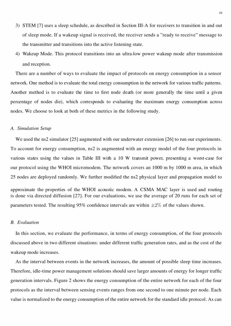
As the interval between events in the network increases, the amount of possible sleep time increases.

Therefore, idle-time power management solutions should save larger amounts of energy for longer traffic

generation intervals. Figure 2 shows the energy consumption of the entire network for each of the four

protocols as the interval between sensing events ranges from one second to one minute per node. Each

value is normalized to the energy consumption of the entire network for the standard idle protocol. As can



11

be seen, the wakeup mode protocol performs almost optimally. This is because the wakeup radio consumes

almost no energy and does not require any additional transmission. STEM, however, due to the probability

that a wakeup signal will be transmitted for some portion of the sleep interval, uses significantly more

energy. Similar curves for times up to 4 hour intervals were roughly the same ( e.g., for a four hour interval,

STEM: 0.76, Wakeup: 0.55, Optimal: 0.54), with STEM always consuming more energy due to increased

transmission times. It is worth pointing out that this represents a worst-case for idle management solutions

since in such a sparse network, virtually all nodes are needed for forwarding traffic.

The primary reason why STEM performs so poorly is that the transmit mode energy consumption of the

acoustic modem is so high (in this case 10 W) that sending the wakeup beacon is very costly. Therefore,

nodes that send the most traffic have much greater costs than the rest of the nodes. The greatest amount

of energy consumed by a node is depicted in Figure 3. Increasing a single node’s energy consumption is

another definite drawback of any sleep cycling solution that increases the transmission time needed to send

data. As can be seen in this figure, certain nodes have their energy expenditure increased dramatically

over the average network energy consumption. This will lead to rapid node failure. If the underwater

sensor networks are sparse, then this will rapidly result in network segmentation. Using a wakeup radio

again keeps the energy consumption very close to optimal.

The main reason why the wakeup mode protocol performs so near optimal for these situations is the

extremely low power used. A fair question to explore is: How low does this power have to be? To answerthis we again look at the same scenario, but this time fix the sensor event frequency at once per minute

per node and vary the power of the wakeup mode between 1 mW and 80 mW (the cost of idle mode).

Figure 4 depicts the total energy consumption of the network. For this traffic rate, the wakeup mode

protocol outperforms STEM for powers lower than about 50 mW. Recall the 500µW figure used early,

even if this number were off by a factor of 10, there would still be very significant gains. As the time

between sensor events increases, this value decreases; however, for events happening more often than

every few hours, the wakeup radio still has the potential to outperform STEM.

Even for wakeup mode levels where STEM outperforms wakeup mode in overall energy consumption,

the highest node energy consumptions are still higher (see Figure 5). This means that the problem

of causing the early death of a node still exists. This is due to the fundamental trade-off used by

unsynchronized sleep cycle solutions (increased transmission time for increased sleep time). When the

transmit and idle costs are close to each other, this trade-off makes sense. However, with the cost associated



12

with transmit power for acoustic modems, this trade-off causes the rapid energy drain of any node that

needs to transmit. Furthermore, to accurately implement a solution like STEM, information about traffic

generation rates is used to optimize the sleep cycle. This information may not be available in highly

dynamic environments. The use of a wakeup mode avoids the need for such information, making the

proposed solution more flexible and robust.

Added delay to transmission is another metric one could use to evaluate such schemes. The added delay

is essentially the sum of the amounts of time that it takes to wake up each node along the path to the

receiver. For wakeup modes, this time is constant with distance and is a function of the one-way transmit

time for the wakeup signal to be received (this can be on the order of a second for long range acoustic

signals) and the time it takes the hardware to power up to receive mode (on the order of microseconds).

Because the propagation time is so long underwater, this delay is dominated by the signal propagation

time which is given by the speed of sound and the distance the signal must travel. It is a fair assumption

that this delay will always be under one second per hop in the network. However, for sleep cycling

solutions, the delay added is both a function of the signal propagation time for the beacon to arrive plus

the average beaconing time. Recall the average beacon time for STEM is given in Equation 1. If we want

the inter-beacon time to be around one second, then the average delay added per hop to a packet will

be 750 ms. This number is added to the propagation delay, which would be equal for both the wakeup

mode and the sleep cycling solutions. Therefore, sleep cycling solutions also add more delay than wakeupmodes and this delay is dependent on the amount of time the node attempt to spend sleeping.

V. CONCLUSIONS AND FUTURE DIRECTIONS

This paper has examined how the differences between acoustic modems and radios affect the design

of idle-time power management schemes. Because idle-time power management schemes that use asyn-

chronous sleep cycling trade off increased transmission time for increased sleep time, their performance

when faced with the extremely high transmit power costs in acoustic modems may be poor.A possibility to implement an ultra-low power wakeup mode in acoustic modems would offer an

alternative to idle-time sleep cycling. We show through simulation that for underwater sensor networks

where the expected traffic generation is less than one packet per node per few hours, the wakeup mode

will save energy over sleep cycling both in terms of total network energy consumed and in terms of the

greatest energy consumption of a single node, thereby increasing the network lifetime by delaying the

first node death.



13

We also show that for a range of costs of wakeup modes, the sleep cycling solutions still perform

poorly. In fact, we show that the wakeup mode solution has the potential to perform almost as well as

the ideal sleep cycle solution, depending on the wakeup mode cost. Additionally, there is work currently

underway to provide wakeup modes consuming less then 10 mW, which would be sufficient to provide

very good performance.

Future work includes analyzing network scenarios with much lower traffic rates (on the order of days)

to find if there is a time when the sleep periods are long enough to cause sleep cycling to outperform

wakeup modes; however such long sleep periods may require longer beacons or large guard times to avoid

packet loss and may contain significant costs that would likely continue to outweigh their gains. For event

driven networks, where traffic is very sparse except during times of certain events, it may be advisable

to combine the techniques, using wakeup mode during times when the event rate is high. Methods of

transitioning between modes without causing large delays for the first event recognition is the subject of

such research.

REFERENCES

[1] I. Akyildiz, D. Pompili, and T. Melodia, “Underwater acoustic sensor networks: Research challenges,” Elsevier’s Ad Hoc Networks,

vol. 3, no. 3, 2005.

[2] J. Heidemann, W. Ye, J. Willis, A. Syed, and Y. Li, “Research challenges and applications for underwater sensor networking,” in

Proceedings of the IEEE Wireless Communications and Networkin Congerence, 2006.

[3] L. Bao and J. J. Garcia-Luna-Aceves, “Topology management in ad hoc networks,” in 4th ACM International Symposium on Mobile

Ad Hoc Networking and Computing (MobiHoc), 2003.

[4] A. Cerpa and D. Estrin, “ASCENT: Adaptive self-configuring sensor networks topologies,” in IEEE INFOCOM , 2002.

[5] B. Chen, K. Jamieson, H. Balakrishnan, and R. Morris, “Span: An energy-efficient coordination algorithm for topology maintenance

in ad hoc wireless networks,” in 7th Annual International Conference on Mobile Computing and Networking (MobiCom), 2001.

[6] R. Kravets and P. Krishnan, “Power management techniques for mobile communication,” in Proc. Fourth ACM International Conference

on Mobile Computing and Networking (MOBICOM’98), 1998.

[7] C. Schurgers, V. Tsiatsis, S. Ganeriwal, and M. Srivastava, “Topology management for sensor networks: Exploiting latency and density,”

in 3rd ACM International Symposium on Mobile Ad Hoc Networking and Computing (MobiHoc) , 2002.

[8] C. Sengul and R. Kravets, “Conserving energy with on-demand topology management,” in Second IEEE International Conference on

Mobile Ad Hoc and Sensor Systems (MASS), November 2005.

[9] J. Wu, F. Dai, M. Gao, and I. Stojmenovic, “On calculating power-aware connected dominating sets for efficient routing in ad hoc

wireless networks,” KICS Journal of Communications and Networks, vol. 4, no. 1, 2002.

[10] Y. Xu, J. Heidemann, and D. Estrin, “Geography-informed energy conservation for ad hoc routing,” in 7th Annual International

Conference on Mobile Computing and Networking (MobiCom), 2001.

[11] R. Zheng and R. Kravets, “On-demand power management for ad hoc networks,” in IEEE INFOCOM , 2003.



14

[12] Cisco, “Cisco Aironet 350 client data sheet,” http://www.cisco.com/.

[13] A. F. Harris III and R. Kravets, “Pincher: A power-saving wireless communication protocol,” University of Illinois at Urbana-Champaign,

Tech. Rep. UIUCDCS-R-2003-2368, 2003.

[14] D. Qiao, S. Choi, A. Jain, and K. G. Shin, “Miser: An optimal low-energy transmission strategy for ieee 802.11a/h,” in Mobicom,

2003.

[15] W. Ye, J. Heidemann, and D. Estrin, “An energy-efficient MAC protocol for wireless sensor networks,” in IEEE INFOCOM , 2002.

[16] M. Zorzi and R. Rao, “Geographic Random Forwarding (GeRaF) for Ad Hoc and Sensor Networks: Multihop Performance,” IEEE

Transactions on Mobile Computing, vol. 2, no. 4, pp. 349–365, 2003.

[17] C. F. Chiasserini and R. R. Rao, “Combining paging with dynamic power management,” in IEEE INFOCOM , 2001.

[18] J. Rabaey, J. Ammer, J. L. da Silva Jr., and D. Patel, “PicoRadio: ad-hoc wireless networking of ubiquitous low-energy sensor/monitor

nodes,” in IEEE Computer Society Annual Workshop on VLSI (WVLSI’00), 2000.

[19] E. Shih, P. Bahl, and M. J. Sinclair, “Wake on wireless: An event driven energy saving strategy of battery operated devices,” in 8th

Annual International Conference on Mobile Computing and Networking (MobiCom), 2002.

[20] Teledyne, “Teledyne-benthos modem,” http://www.rdinstruments.com/nemo.

[21] I. Link-Quest, “Link-quest modem,” http://www.link-quest.com/html/models1.htm.

[22] L. Freitag, M. Grund, S. Singh, J. Partan, P. Koski, and K. Ball, “The WHOI micro-modem: An acoustic communications and navigation

system for multiple platforms,” http://www.whoi.edu, 2005.

[23] M. Molins and M. Stojanovic, “Slotted FAMA: a MAC protocol for underwater acoustic networks,” in Proc. IEEE Oceans Conference,

2006.

[24] M. Stojanovic, “Optimization of a data link protocol for underater acoustic networks,” in Proc. IEEE Oceans Conference, 2005.

[25] ns2 Network Simulator, http://www.isi.edu/nsnam/ns/.

[26] A. F. Harris and M. Zorzi, “Modeling the underwater acoustic channel in ns2,” in ACM International Workshop on Network Simulation

Tools (NSTools), 2007.

[27] C. Intanagonwiwat, R. Govindan, and D. Estrin, “Directed diffusion: A scalable and robust communication paradigm for sensor

networks,” in MobiCom, 2000.

[28] J.-R. Jiang, Y.-C. Tseng, C.-S. Hsu, and T.-H. Lai, “Quorum-based asynchronous power-saving protocols for IEEE 802.11 ad hoc

networks,” in International Conference on Parallel Processing (ICPP), 2003.

[29] XBOW, “2nd generation micamote,” http://www.xbow.com.





16

0 10 20 30 40 50 600.6

0.65

0.7

0.75

0.8

0.85

0.9

0.95

1

1.05

1.1

Generation interval (s)

E n e r g y C o n s u m p t i o n ( n o r m a l i z e d t o I d l e )

Optimal

STEM

Wakeup

Idle

Fig. 2. Total energy consumption of the network vs. traffic generation interval

0 10 20 30 40 50 600.8

0.9

1

1.1

1.2

1.3

1.4

1.5

1.6

Generation interval (s)

E n e r g y C o n s u m p t i o n ( n o r m a l i z e d t o I d l e )

Optimal

Idle

Wakeup

STEM

Fig. 3. Highest energy consumption of a node vs. traffic generation interval

0 10 20 30 40 50 60 70 80

0.65

0.7

0.75

0.8

0.85

0.9

0.95

1

1.05

1.1

Wakeup Power (mW)

E n e r g y C o n s u m p t i o n ( n o

r m a l i z e d t o I d l e )

Idle

Optimal

Wakeup

STEM

Fig. 4. Total energy consumption of network vs. wakeup mode cost



17

0 10 20 30 40 50 60 70 800.7

0.8

0.9

1

1.1

1.2

1.3

1.4

1.5

1.6

1.7

Wakeup Power (mW)

E n e r g y C o n s u m p t i o n ( n o r m a l i z e d t o i d l e )

Idle

Optimal

Wakeup

STEM

Fig. 5. Highest energy consumption of a node vs. wakeup mode cost

Documents

Elsevier Al