Entanglement in a Quantum Annealing Processor

T. Lanting,1,* A. J. Przybysz,1 A. Yu. Smirnov,1 F. M. Spedalieri,2,3 M. H. Amin,1,4 A. J. Berkley,1 R. Harris,1 F. Altomare,1

S. Boixo,2,5 P. Bunyk,1 N. Dickson,1,† C. Enderud,1 J. P. Hilton,1 E. Hoskinson,1 M.W. Johnson,1 E. Ladizinsky,1

N. Ladizinsky,1 R. Neufeld,1 T. Oh,1 I. Perminov,1 C. Rich,1 M. C. Thom,1 E. Tolkacheva,1 S. Uchaikin,1,6

A. B. Wilson,1 and G. Rose11D-Wave Systems Inc., 3033 Beta Avenue, Burnaby, British Columbia, Canada V5G 4M9

2Information Sciences Institute, University of Southern California, Los Angeles, California 90089, USA3Center for Quantum Information Science and Technology, University of Southern California,

Los Angeles, California 90089, USA4Department of Physics, Simon Fraser University, Burnaby, British Columbia, Canada V5A 1S6

5Google, 340 Main Street, Venice, California 90291, USA6National Research Tomsk Polytechnic University, 30 Lenin Avenue, Tomsk, 634050, Russia

(Received 13 December 2013; published 29 May 2014)

Entanglement lies at the core of quantum algorithms designed to solve problems that are intractable byclassical approaches. One such algorithm, quantum annealing (QA), provides a promising path to apractical quantum processor. We have built a series of architecturally scalable QA processors consisting ofnetworks of manufactured interacting spins (qubits). Here, we use qubit tunneling spectroscopy to measurethe energy eigenspectrum of two- and eight-qubit systems within one such processor, demonstratingquantum coherence in these systems. We present experimental evidence that, during a critical portion ofQA, the qubits become entangled and entanglement persists even as these systems reach equilibrium with athermal environment. Our results provide an encouraging sign that QA is a viable technology for large-scale quantum computing.

DOI: 10.1103/PhysRevX.4.021041 Subject Areas: Quantum Physics,Quantum Information, Superconductivity

I. INTRODUCTION

The past decade has been exciting for the field ofquantum computation. A wide range of physical imple-mentations of architectures that promise to harness quan-tum mechanics to perform computation have been studied[1–3]. Scaling these architectures to build practical pro-cessors with many millions to billions of qubits will bechallenging [4,5]. A simpler architecture, designed toimplement a single quantum algorithm such as quantumannealing (QA), provides a more practical approach in thenear term [6,7]. However, one of the main features thatmakes such an architecture scalable, namely, a limitednumber of low-bandwidth external control lines [8], pro-hibits many typical characterization measurements used instudying prototype universal quantum computers [9–14].These constraints make it challenging to experimentallydetermine whether a scalable QA architecture, one that is

inevitably coupled to a thermal environment, is capable ofgenerating entangled states [15–18]. A demonstration ofentanglement is considered to be a critical milestone for anyapproach to building a quantum computing technology.Herein, we demonstrate an experimental method to detectentanglement in subsections of a quantum annealingprocessor to address this fundamental question.

II. QUANTUM ANNEALING

QA is designed to find the low-energy configurations ofsystems of interacting spins. Awide variety of optimizationproblems naturally map onto this physical system [19–22].A QA algorithm is described by a time-dependentHamiltonian for a set of N spins, i ¼ 1;…; N,

HSðsÞ ¼ EðsÞHP −1

2

Xi

ΔðsÞσxi ; (1)

where the dimensionless HP is

HP ¼ −Xi

hiσzi þ

Xi<j

Jijσziσ

zj (2)

and σx;zi are Pauli matrices for the ith spin. The energyscales Δ and E are the transverse and longitudinal energies

*tlanting@dwavesys.com†Present address: Side Effects Software, 1401-123 Front Street

West, Toronto, Ontario, Canada.

Published by the American Physical Society under the terms ofthe Creative Commons Attribution 3.0 License. Further distri-bution of this work must maintain attribution to the author(s) andthe published article’s title, journal citation, and DOI.

PHYSICAL REVIEW X 4, 021041 (2014)

2160-3308=14=4(2)=021041(14) 021041-1 Published by the American Physical Society

of the spins, respectively, and the biases hi and couplingsJij encode a particular optimization problem. The time-dependent variation of Δ and E is parametrized by s≡ t=tfwith time t ∈ ½0; tf� and total run (anneal) time tf. QA isperformed by first setting Δ ≫ E, which results in a groundstate into which the spins can be easily initialized [6]. ThenΔ is reduced and E is increased until E ≫ Δ. At this point,the system Hamiltonian is dominated by HP, whichrepresents the encoded optimization problem. At the endof the evolution, a ground state ofHP represents the lowestenergy configuration for the problem Hamiltonian and thusa solution to the optimization problem.

III. QUANTUM ANNEALING PROCESSOR

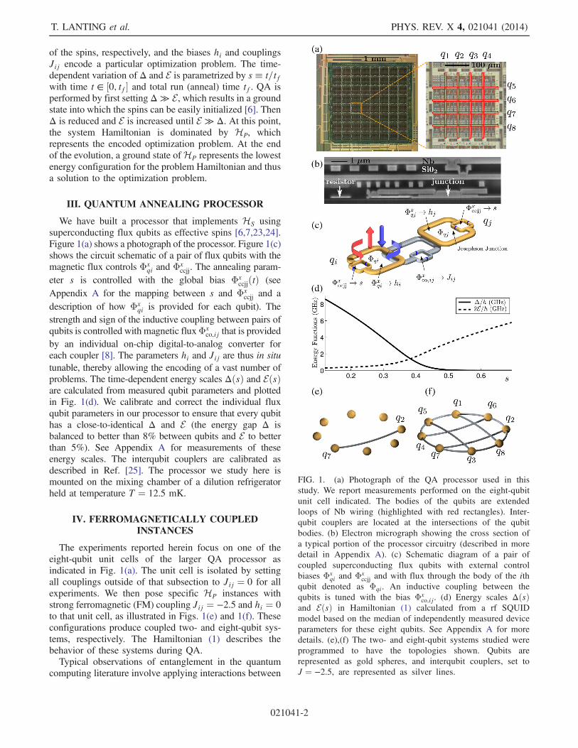
We have built a processor that implements HS usingsuperconducting flux qubits as effective spins [6,7,23,24].Figure 1(a) shows a photograph of the processor. Figure 1(c)shows the circuit schematic of a pair of flux qubits with themagnetic flux controls Φx

qi and Φxccjj. The annealing param-

eter s is controlled with the global bias ΦxccjjðtÞ (see

Appendix A for the mapping between s and Φxccjj and a

description of how Φxqi is provided for each qubit). The

strength and sign of the inductive coupling between pairs ofqubits is controlled with magnetic fluxΦx

co;ij that is providedby an individual on-chip digital-to-analog converter foreach coupler [8]. The parameters hi and Jij are thus in situtunable, thereby allowing the encoding of a vast number ofproblems. The time-dependent energy scales ΔðsÞ and EðsÞare calculated from measured qubit parameters and plottedin Fig. 1(d). We calibrate and correct the individual fluxqubit parameters in our processor to ensure that every qubithas a close-to-identical Δ and E (the energy gap Δ isbalanced to better than 8% between qubits and E to betterthan 5%). See Appendix A for measurements of theseenergy scales. The interqubit couplers are calibrated asdescribed in Ref. [25]. The processor we study here ismounted on the mixing chamber of a dilution refrigeratorheld at temperature T ¼ 12.5 mK.

IV. FERROMAGNETICALLY COUPLEDINSTANCES

The experiments reported herein focus on one of theeight-qubit unit cells of the larger QA processor asindicated in Fig. 1(a). The unit cell is isolated by settingall couplings outside of that subsection to Jij ¼ 0 for allexperiments. We then pose specific HP instances withstrong ferromagnetic (FM) coupling Jij ¼ −2.5 and hi ¼ 0to that unit cell, as illustrated in Figs. 1(e) and 1(f). Theseconfigurations produce coupled two- and eight-qubit sys-tems, respectively. The Hamiltonian (1) describes thebehavior of these systems during QA.Typical observations of entanglement in the quantum

computing literature involve applying interactions between

FIG. 1. (a) Photograph of the QA processor used in thisstudy. We report measurements performed on the eight-qubitunit cell indicated. The bodies of the qubits are extendedloops of Nb wiring (highlighted with red rectangles). Inter-qubit couplers are located at the intersections of the qubitbodies. (b) Electron micrograph showing the cross section ofa typical portion of the processor circuitry (described in moredetail in Appendix A). (c) Schematic diagram of a pair ofcoupled superconducting flux qubits with external controlbiases Φx

qi and Φxccjj and with flux through the body of the ith

qubit denoted as Φqi. An inductive coupling between thequbits is tuned with the bias Φx

co;ij. (d) Energy scales ΔðsÞand EðsÞ in Hamiltonian (1) calculated from a rf SQUIDmodel based on the median of independently measured deviceparameters for these eight qubits. See Appendix A for moredetails. (e),(f) The two- and eight-qubit systems studied wereprogrammed to have the topologies shown. Qubits arerepresented as gold spheres, and interqubit couplers, set toJ ¼ −2.5, are represented as silver lines.

T. LANTING et al. PHYS. REV. X 4, 021041 (2014)

021041-2

qubits, removing these interactions, and then performingmeasurements. Such an approach is well suited to gate-model architectures (see, e.g., Ref. [11]). During QA,however, the interaction between qubits is determined bythe particular instance of HP, in this case, a stronglyferromagnetic instance, and cannot be removed. In thisway, systems of qubits undergoing QA have much more incommon with condensed-matter systems, such as quantummagnets, for which interactions cannot be turned off.Indeed, a growing body of recent theoretical and exper-imental work suggests that entanglement plays a centralrole in many of the macroscopic properties of condensed-matter systems [26–32]. Here, we introduce otherapproaches to quantifying entanglement that are suitedto QA processors. We establish experimentally that thetwo- and eight-qubit systems, comprising macroscopic

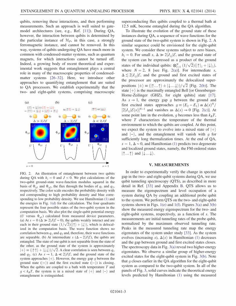
superconducting flux qubits coupled to a thermal bath at12.5 mK, become entangled during the QA algorithm.To illustrate the evolution of the ground state of these

instances during QA, a sequence of wave functions for theground state of the two-qubit system is shown in Fig. 2. Asimilar sequence could be envisioned for the eight-qubitsystem. We consider these systems subject to zero biases,hi ¼ 0. For small s, Δ ≫ 2jJijjE, and the ground state ofthe system can be expressed as a product of the groundstates of the individual qubits: ⊗N

i¼1 ð1=ffiffiffi2

p Þðj↑ii þ j↓iiÞ,where N ¼ 2, 8 [see Fig. 2(a)]. For intermediate s,Δ≲ 2jJijjE, and the ground and first excited states ofthe processor are approximately the delocalized super-positions j�i≡ ðj↑…↑i � j↓…↓iÞ= ffiffiffi

2p

[Fig. 2(b)]. Thestate jþi is the maximally entangled Bell [or Greenberger-Horne-Zeilinger (GHZ), for eight qubits] state [17].As s → 1, the energy gap g between the ground andfirst excited states approaches g≡ ðE2 − E1Þ ∝ ΔðsÞN=½2jJijjEðsÞ�N−1 and vanishes as ΔðsÞ → 0 [Fig. 2(c)]. Atsome point late in the evolution, g becomes less than kBT,where T characterizes the temperature of the thermalenvironment to which the qubits are coupled. At this point,we expect the system to evolve into a mixed state of jþiand j−i, and the entanglement will vanish with g forsufficiently long thermalization times. At the end of QA,s ¼ 1, Δ ∼ 0, and Hamiltonian (1) predicts two degenerateand localized ground states, namely, the FM-ordered statesj↑…↑i and j↓…↓i.

V. MEASUREMENTS

In order to experimentally verify the change in spectralgap in the two- and eight-qubit systems during QA, we usequbit tunneling spectroscopy (QTS), as described in moredetail in Ref. [33] and Appendix B. QTS allows us tomeasure the eigenspectrum and level occupation of asystem during QA by coupling an additional probe qubitto the system. We perform QTS on the two- and eight-qubitsystems shown in Figs. 1(e) and 1(f). Figures 3(a) and 3(b)show the measured energy eigenspectrum for the two- andeight-qubit systems, respectively, as a function of s. Themeasurements are initial tunneling rates of the probe qubit,normalized by the maximum observed tunneling rate.Peaks in the measured tunneling rate map the energyeigenstates of the system under study [33]. As the systemevolves (increasing s), ΔðsÞ in Hamiltonian (1) decreasesand the gap between ground and first excited states closes.The spectroscopy data in Fig. 3(a) reveal two higher-energyeigenstates. We observe a similar group of higher-energyexcited states for the eight-qubit system in Fig. 3(b). Notethat g closes earlier in the QA algorithm for the eight-qubitsystem as compared to the two-qubit system. In all of thepanels of Fig. 3, solid curves indicate the theoretical energylevels predicted by Hamiltonian (1) using the measured

(a) (b) (c)

FIG. 2. An illustration of entanglement between two qubitsduring QA with hi ¼ 0 and J < 0. We plot calculations of thetwo-qubit ground-state wave-function modulus squared in thebasis of Φq1 and Φq2, the flux through the bodies of q1 and q2,respectively. The color scale encodes the probability density withred corresponding to high probability density and blue corre-sponding to low probability density. We use Hamiltonian (1) andthe energies in Fig. 1(d) for the calculation. The four quadrantsrepresent the four possible states of the two-qubit system in thecomputation basis. We also plot the single-qubit potential energy(U versus Φq1) calculated from measured device parameters.(a) At s ¼ 0 (Δ ≫ 2jJjE ∼ 0), the qubits weakly interact and areeach in their ground state ð1= ffiffiffi

2p Þðj↑i þ j↓iÞ, which is delocal-

ized in the computation basis. The wave function shows nocorrelation between q1 and q2 and, therefore, their wave functionsare separable. (b) At intermediate s (Δ ∼ 2jJjE), the qubits areentangled. The state of one qubit is not separable from the state ofthe other, as the ground state of the system is approximatelyjþi≡ ðj↑↑i þ j↓↓iÞ= ffiffiffi

2p

. A clear correlation is seen between q1and q2. (c) As s → 1, Δ ≪ 2jJjE, and the ground state of thesystem approaches jþi. However, the energy gap g between theground state (jþi) and the first excited state (j−i) is closing.When the qubits are coupled to a bath with temperature T andg < kBT, the system is in a mixed state of jþi and j−i andentanglement is extinguished.

ENTANGLEMENT IN A QUANTUM ANNEALING PROCESSOR PHYS. REV. X 4, 021041 (2014)

021041-3

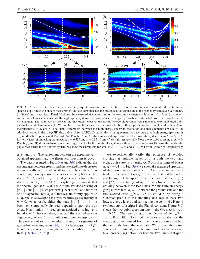
ΔðsÞ and EðsÞ. The agreement between the experimentallyobtained spectrum and the theoretical spectrum is good.The data presented in Figs. 3(a) and 3(b) indicate that the

spectral gap between ground and first excited state decreasesmonotonically with s when all hi ¼ 0. Under these biasconditions, these systems possess Z2 symmetry between thestates j↑…↑i and j↓…↓i. The degeneracy between thesestates is lifted by finite ΔðsÞ. To explicitly demonstrate thatthe spectral gap at hi ¼ 0 is due to the avoided crossing ofj↑…↑i and j↓…↓i, we performQTS at fixed s as a functionof a “diagnostic” bias hi ≠ 0 that was uniformly applied toall qubits, thus sweeping the systems through degeneracy athi ¼ 0. As a result, either the state j↑…↑i or j↓…↓ibecomes energetically favored, depending upon the signof hi. Hamiltonian (1) predicts an avoided crossing, as afunction of hi, between the ground and first excited states atdegeneracy, where hi ¼ 0, with a minimum energy gap g.The presence of such an avoided crossing is a signature ofground-state entanglement [14,35]. For large gaps, g > kBT,there is persistent entanglement at equilibrium (seeRefs. [18,26,28,29,31]).

We experimentally verify the existence of avoidedcrossings at multiple values of s in both the two- andeight-qubit systems by using QTS across a range of biaseshi ∈ f−4; 4g. In Fig. 3(c), we show the measured spectrumof the two-qubit system at s ¼ 0.339 up to an energy of6 GHz for a range of bias hi. The ground states at the far leftand far right of the spectrum are the localized states j↓↓iand j↑↑i, respectively. At hi ¼ 0, we observe an avoidedcrossing between these two states. We measure an energygap g at zero bias, hi ¼ 0, between the ground state and thefirst excited state, g=h ¼ 1.75� 0.08 GHz, by fitting aGaussian profile to the tunneling rate data at these twolowest-energy levels and subtracting the centroids. Here, h(without any subscript) is the Planck constant. Figure 3(d)shows the two-qubit spectrum later in the QA algorithm, ats ¼ 0.351. The energy gap has decreased to g=h ¼1.21� 0.06 GHz. Note that the error estimates for theenergy gaps are derived from the uncertainty in extractingthe centroids from the rate data. We discuss the actualsource of the underlying Gaussian widths (the observedlevel broadening) below. For both the two- and eight-qubit

(a) (b)

(c) (d) (e) (f)

FIG. 3. Spectroscopic data for two- and eight-qubit systems plotted in false color (color indicates normalized qubit tunnelspectroscopy rates). A nonzero measurement (false color) indicates the presence of an eigenstate of the probed system at a given energy(ordinate) and s (abscissa). Panel (a) shows the measured eigenspectrum for the two-qubit system as a function of s. Panel (b) shows asimilar set of measurements for the eight-qubit system. The ground-state energy E1 has been subtracted from the data to aid invisualization. The solid curves indicate the theoretical expectations for the energy eigenvalues using independently calibrated qubitparameters and Hamiltonian (1). We emphasize that the solid curves are not a fit, but rather a prediction based on Hamiltonian (1) andmeasurements of Δ and E. The slight differences between the high-energy spectrum prediction and measurements are due to theadditional states in the rf SQUID flux qubits. A full rf SQUID model that is in agreement with the measured high-energy spectrum isexplored in the Supplemental Material [34]. Panels (c) and (d) show measured eigenspectra of the two-qubit system versus h1 ¼ h2 ≡ hifor two values of annealing parameter s, s ¼ 0.339 and s ¼ 0.351 from left to right, respectively. Note the avoided crossing at hi ¼ 0.Panels (e) and (f) show analogous measured eigenspectra for the eight-qubit system (with h1 ¼ � � � ¼ h8 ≡ hi). Because the eight-qubitgap closes earlier in QA for this system, we show measurements for smaller s, s ¼ 0.271 and s ¼ 0.284 from left to right, respectively.

T. LANTING et al. PHYS. REV. X 4, 021041 (2014)

021041-4

systems, we confirm that the expectation values of σz for alldevices change sign as the system moves through theavoided crossing (see Figs. 1–3 of the SupplementalMaterial [34] and Ref. [35]).Figures 3(e) and 3(f) show similar measurements of the

spectrum of eight coupled qubits at s ¼ 0.271 and s ¼0.284 for a range of biases hi. Again, we observe anavoided crossing at hi ¼ 0. The measured energy gaps ats ¼ 0.271 and 0.284 are g=h ¼ 2.2� 0.08 GHz andg=h ¼ 1.66� 0.06 GHz, respectively. Although the eight-qubit gaps in Figs. 3(e) and 3(f) are close to the two-qubitgaps in Figs. 3(c) and 3(d), they are measured at quitedifferent values of the annealing parameter s. As expected,the eight-qubit gap is closing earlier in the QA algorithm ascompared to the two-qubit gap. The solid curves inFigs. 3(c)–3(f) indicate the theoretical energy levels pre-dicted by Hamiltonian (1) and measurements of ΔðsÞ andEðsÞ. Again, the agreement between the experimentallyobtained spectra and the theoretical spectra is good.For the early and intermediate parts of QA, the energy

gap g is larger than temperature, g ≫ kBT, for both thetwo- and eight-qubit systems. We expect that if we holdthe systems at these s, then the only eigenstate withsignificant occupation will be the ground state. Weconfirm this by using QTS in the limit of long tunnelingtimes to probe the occupation fractions. Details are

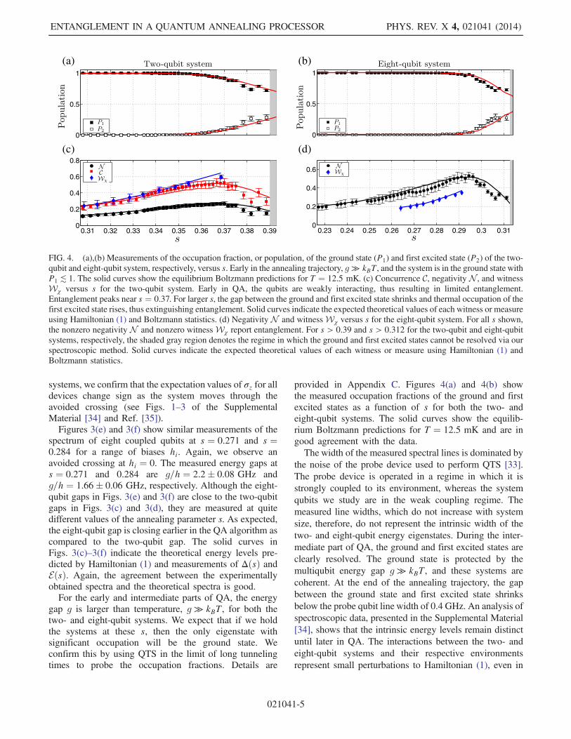
provided in Appendix C. Figures 4(a) and 4(b) showthe measured occupation fractions of the ground and firstexcited states as a function of s for both the two- andeight-qubit systems. The solid curves show the equilib-rium Boltzmann predictions for T ¼ 12.5 mK and are ingood agreement with the data.The width of the measured spectral lines is dominated by

the noise of the probe device used to perform QTS [33].The probe device is operated in a regime in which it isstrongly coupled to its environment, whereas the systemqubits we study are in the weak coupling regime. Themeasured line widths, which do not increase with systemsize, therefore, do not represent the intrinsic width of thetwo- and eight-qubit energy eigenstates. During the inter-mediate part of QA, the ground and first excited states areclearly resolved. The ground state is protected by themultiqubit energy gap g ≫ kBT, and these systems arecoherent. At the end of the annealing trajectory, the gapbetween the ground state and first excited state shrinksbelow the probe qubit line width of 0.4 GHz. An analysis ofspectroscopic data, presented in the Supplemental Material[34], shows that the intrinsic energy levels remain distinctuntil later in QA. The interactions between the two- andeight-qubit systems and their respective environmentsrepresent small perturbations to Hamiltonian (1), even in

0

0.5

1

0.31 0.32 0.33 0.34 0.35 0.36 0.37 0.38 0.390

0.2

0.4

0.6

0.8

0

0.5

1

0.23 0.24 0.25 0.26 0.27 0.28 0.29 0.3 0.310

0.2

0.4

0.6

(a) (b)

(c) (d)

FIG. 4. (a),(b) Measurements of the occupation fraction, or population, of the ground state (P1) and first excited state (P2) of the two-qubit and eight-qubit system, respectively, versus s. Early in the annealing trajectory, g ≫ kBT, and the system is in the ground state withP1 ≲ 1. The solid curves show the equilibrium Boltzmann predictions for T ¼ 12.5 mK. (c) Concurrence C, negativity N , and witnessWχ versus s for the two-qubit system. Early in QA, the qubits are weakly interacting, thus resulting in limited entanglement.Entanglement peaks near s ¼ 0.37. For larger s, the gap between the ground and first excited state shrinks and thermal occupation of thefirst excited state rises, thus extinguishing entanglement. Solid curves indicate the expected theoretical values of each witness or measureusing Hamiltonian (1) and Boltzmann statistics. (d) Negativity N and witness Wχ versus s for the eight-qubit system. For all s shown,the nonzero negativity N and nonzero witness Wχ report entanglement. For s > 0.39 and s > 0.312 for the two-qubit and eight-qubitsystems, respectively, the shaded gray region denotes the regime in which the ground and first excited states cannot be resolved via ourspectroscopic method. Solid curves indicate the expected theoretical values of each witness or measure using Hamiltonian (1) andBoltzmann statistics.

ENTANGLEMENT IN A QUANTUM ANNEALING PROCESSOR PHYS. REV. X 4, 021041 (2014)

021041-5

the regime in which entanglement is beginning to fall due tothermal mixing.

VI. ENTANGLEMENT DETECTION

The tunneling spectroscopy data show that, midwaythrough QA, both the two- and eight-qubit systems haveavoided crossings with the expected gap g ≫ kBT and haveground-state occupation P1 ≃ 1. While observation of anavoided crossing is evidence for the presence of anentangled ground state [35], we can make this observationmore quantitative with entanglement measures andwitnesses.For a large part of the QA algorithm, the two- and eight-

qubit systems are in their ground states with high occupa-tion fraction. We, therefore, begin the analysis with asusceptibility-based witness Wχ , which detects ground-state entanglement. This witness does not require explicitknowledge of Hamiltonian (1), but requires a nondegen-erate ground state, confirmed with the avoided crossingsshown in Fig. 3, and high occupation fraction of the groundstate, confirmed early in QA by the measurements ofP1 ≃ 1 shown in Fig. 4. We then perform measurementsof all available linear cross susceptibilities

χij ≡ dhσzi i=d ~hj; (3)

where hσzi i is the expectation value of σzi for the ith qubitand ~hj ¼ Ehj is a bias applied to the jth qubit. Themeasurements are performed at the degeneracy point (inthe middle of the avoided crossings), where the classicalcontribution to the cross susceptiblity is zero.From these measurements, we calculateWχ as defined in

Ref. [35] (see Appendix D for more details). A nonzerovalue of this witness detects ground-state entanglement,and global entanglement in the case of the eight-qubitsystem (meaning every possible bipartition of the eight-qubit system is entangled). Figures 4(c) and 4(d) show Wχ

for the two- and eight-qubit systems. Note that for twoqubits at degeneracy, Wχ coincides with ground-stateconcurrence. These results indicate that the two- andeight-qubit systems are entangled midway through QA.Note also that a susceptibility-based witness has a closeanalogy to susceptibility-based measurements of nano-magnetic systems that also report strong nonclassicalcorrelations [29,31].The occupation fraction measurements shown in Fig. 4

indicate that midway through QA, the first excited state ofthese systems is occupied as the energy gap g begins toapproach kBT. The systems are no longer in the groundstate but, rather, in a mixed state. To detect the presence ofmixed-state entanglement, we need knowledge about thedensity matrix of these systems. Occupation fractionmeasurements provide measurements of the diagonalelements of the density matrix in the energy basis. Weassume that the density matrix has no off-diagonal elements

in the energy basis (they decay on time scales of severalnanoseconds). We relax this assumption below. PopulationsP1 and P2 plotted in Figs. 4(a) and 4(b) indicate that thesystem occupies these states with almost 100% probability.This means that the density matrix can be written in theform ρ ¼ P

2i¼1 Pijψ iihψ ij, where jψ ii represents the ith

eigenstate of Hamiltonian (1).We use the density matrix to calculate standard entan-

glement measures, Wootters’ concurrence C [18] for thetwo-qubit system, and negativity N [16,36] for thetwo- and eight-qubit system. For the maximally entangledtwo-qubit Bell state, we note that C ¼ 1 and N ¼ 0.5.Figure 4(c) shows C as a function of s. Midway throughQA, we measure a peak concurrence C ¼ 0.53� 0.05,indicating significant entanglement in the two-qubit sys-tem. This value of C corresponds to an entanglement offormation Ef ¼ 0.388 (see Refs. [16,18] for definitions).This is comparable to the level of entanglement,Ef ¼ 0.378, obtained in Ref. [11]. Because concurrenceC is not applicable to more than two qubits, we usenegativity N to detect entanglement in the eight-qubitsystem. For N > 2, N A;B is defined on a particularbipartition of the system into subsystems A and B. Wedefine N to be the geometric mean of this quantity acrossall possible bipartitions. A nonzero N indicates thepresence of global entanglement. Figures 4(c) and 4(d)show the negativity calculated with measured P1 and P2

(and with the measured Hamiltonian parameters Δ andEJij) as a function of s for the two- and eight-qubit systems.The eight-qubit system has nonzero N for s < 0.315, thusindicating the presence of mixed-state global entanglement.Both concurrence C and negativityN decrease later in QA,where the first excited state approaches the ground state andbecomes thermally occupied. The experimental values ofthese entanglement measures are in agreement with thetheoretical predictions (solid lines in Fig. 4). The error barsin Figs. 4(c) and 4(d) represent uncertainties in themeasurements of P1ðsÞ, P2ðsÞ, ΔðsÞ, and EðsÞ.As stated above, the calculation of C and N relies on the

assumption that the off-diagonal terms in the density matrixdecay on time scales of several nanoseconds. We removethis assumption and demonstrate entanglement through theuse of another witness WAB, defined on some bipartitionA-B of the eight-qubit system. The witness, described inAppendix D, is designed in such a way that Tr½WABσ� ≥ 0for all separable states σ. When Tr½WABρðsÞ� < 0, the stateρðsÞ is entangled. Measurements of populations P1 and P2

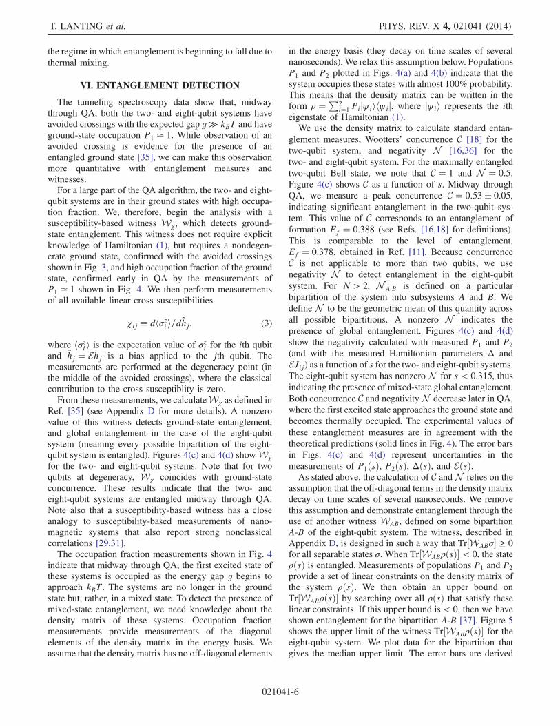
provide a set of linear constraints on the density matrix ofthe system ρðsÞ. We then obtain an upper bound onTr½WABρðsÞ� by searching over all ρðsÞ that satisfy theselinear constraints. If this upper bound is < 0, then we haveshown entanglement for the bipartition A-B [37]. Figure 5shows the upper limit of the witness Tr½WABρðsÞ� for theeight-qubit system. We plot data for the bipartition thatgives the median upper limit. The error bars are derived

T. LANTING et al. PHYS. REV. X 4, 021041 (2014)

021041-6

from a Monte Carlo analysis wherein we used the exper-imental uncertainties in Δ and J to estimate the uncertaintyin Tr½WABρ�. We also plot data for the two partitions thatgive the largest and smallest upper limits. For all values ofthe annealing parameter s, except for the last two points,upper limits from all possible bipartitions of the eight-qubitsystem are below zero. In this annealing range, the eight-qubit system is globally entangled.

VII. CONCLUSIONS

In summary, we provide experimental evidence for thepresence of quantum coherence and entanglement withinsubsets of qubits inside a quantum annealing processorduring its operation. Our conclusion is based on four levelsof evidence: (a) the observation of two- and eight- qubitavoided crossings with a multiqubit energy gap g ≫ kBT;(b) the witness Wχ, calculated with measured crosssusceptibilities and coupling energies, which reportsground-state entanglement of the two- and eight-qubitsystems [note that these two levels of evidence do notrequire explicit knowledge of Hamiltonian (1)]; (c) themeasurements of energy eigenspectra and equibrium occu-pation fractions during QA, which allow us to useHamiltonian (1) to reconstruct the density matrix, withsome weak assumptions, and calculate concurrence andnegativity (these standard measures of entanglement report

nonclassical correlations in the two- and eight-qubit sys-tems); (d) the entanglement witness WAB, which is calcu-lated with the measured Hamiltonian and with constraintsprovided by the measured populations of the ground andthe first excited states (this witness reports global entan-glement of the eight-qubit system midway through the QAalgorithm).The observed entanglement is persistent at thermal

equilibrium, an encouraging result as any practical hard-ware designed to run a quantum algorithm will be inevi-tably coupled to a thermal environment. The experimentaltechniques we discuss provide measurements of energylevels, and their populations, for arbitrary configurations ofHamiltonian parametersΔ, hi, Jij during the QA algorithm.The main limitation of the technique is the spectral width ofthe probe device. Improved designs of this device willallow much larger systems to be studied. Our measure-ments represent an effective approach for exploring the roleof quantum mechanics in QA processors and ultimately tounderstanding the fundamental power and capability ofquantum annealing.

ACKNOWLEDGMENTS

We thank C. Williams, P. Love, and J. Whittaker foruseful discussions. We acknowledge F. Cioata and P. Spearfor the design and maintenance of electronics controlsystems, J. Yao for fabrication support, and D. Bruce, P.deBuen, M. Gullen, M. Hager, G. Lamont, L. Paulson, C.Petroff, and A. Tcaciuc for technical support. F. M. S. wassupported by DARPA, under Contract No. FA8750-13-2-0035.

APPENDIX A: QA PROCESSOR DESCRIPTION

1. Chip description

The experiments discussed in herein were performed ona sample fabricated with a process consisting of a standardNb/AlOx/Nb trilayer, a TiPt resistor layer, planarized SiO2

dielectric layers, and six Nb wiring layers. The circuitdesign rules include a minimum linewidth of 0.25 μm and0.6-μm-diameter Josephson junctions. The processor chipis a network of densely connected eight-qubit unit cells thatare more sparsely connected to each other (see Fig. 1 forphotographs of the processor). We report measurementsmade on qubits from one of these unit cells. The chip ismounted on the mixing chamber of a dilution refrigeratorinside an Al superconducting shield and temperaturecontrolled at 12.5 mK.

2. Qubit parameters

The processor facilitates quantum annealing of com-pound-compound Josephson junction rf SQUID flux qubits[38]. The qubits are controlled via the external flux biasesΦx

qi andΦxccjj, which allow us to treat them as effective spins

(see Fig. 1). Pairs of qubits interact through tunable

0.24 0.26 0.28 0.3−0.5

−0.4

−0.3

−0.2

−0.1

0

0.1

0.2

FIG. 5. Upper limit of the quantity Tr½WABρ� versus s forseveral bipartitions A − B of the eight-qubit system. When thisquantity is less than 0, the system is entangled with respect to thisbipartition. The solid dots show the upper limit on Tr½WABρ� forthe median bipartition. The open dots above and below these arederived from the two bipartitions that give the highest and lowestupper limits on Tr½WABρ�, respectively. For the points at s > 0.3,the measurements of P1 and P2 do not constrain ρ enough tocertify entanglement.

ENTANGLEMENT IN A QUANTUM ANNEALING PROCESSOR PHYS. REV. X 4, 021041 (2014)

021041-7

inductive couplings [25]. The system can be described withthe time-dependent QA Hamiltonian,

HSðsÞ ¼ EðsÞ�−XNi

hiσzi þ

Xi<j

Jijσziσ

zj

�−1

2ΔðsÞ

XNi

σxi ;

(A1)

where σx;zi are Pauli matrices for the ith qubit, i ¼ 1;…; N.The energy scales Δ and E are the transverse and longi-tudinal energies of the spins, respectively, and the unitlessbiases hi and couplings Jij encode a particular optimization

problem. We define ~hi ≡ Ehi and ~Jij ≡ EJij. We map theannealing parameter s for this particular chip to a range ofΦx

ccjj with the relation

s≡ ðΦxccjjðtÞ − Φx

ccjj;initialÞ=ðΦxccjj;final − Φx

ccjj;initialÞ ¼ t=tf;

(A2)

where tf is the total anneal time. We implement QA for thisprocessor by ramping the external control Φx

ccjjðtÞ fromΦx

ccjj;initial ¼ 0.596 Φ0 (s ¼ 0) at t ¼ 0 to Φxccjj;final ¼ 0.666

Φ0 (s ¼ 1) at t ¼ tf. The energy scale E ≡Meff jIpqðsÞj2 isset by the s-dependent persistent current of the qubit jIpqðsÞjand the maximum mutual inductance between qubitsMeff ¼ 1.37 pH [8]. The transverse term in Hamiltonian(A1), ΔðsÞ, is the energy gap between the ground and firstexcited state of an isolated rf SQUID at zero bias. Δ alsochanges with annealing parameter s. Φx

qiðtÞ is provided by aglobal external magnetic flux bias along with local in situtunable DAC that tunes the coupling strength of this globalbias into individual qubits and thus allows us to specifyindividual biases hi. The coupling energy between the ithand jth qubit is set with a local in situ tunable DAC thatcontrols Φx

co;ij.The main quantities associated with a flux qubit, Δ and

jIpq j, primarily depend on macroscopic rf SQUID param-eters: junction critical current Ic, qubit inductance Lq, andqubit capacitance Cq. We calibrate all of these parameterson this chip as described in Refs. [6,8]. We calibrate allinterqubit coupling elements across their available tuningrange from 1.37 pH to −3.7 pH, as described in Ref. [25].We correct for variations in qubit parameters with on-chipcontrol as described in Ref. [8]. This allows us to match jIpq jand Δ across all qubits throughout the annealing trajectory.

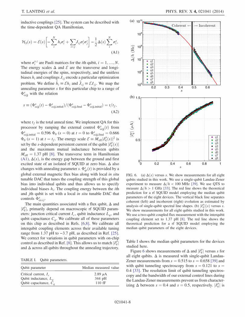
Table I shows the median qubit parameters for the devicesstudied here.Figure 6 shows measurements of Δ and jIpq j versus s for

all eight qubits. Δ is measured with single-qubit Landau-Zener measurements from s ¼ 0.515 to s ¼ 0.658 [39] andwith qubit tunneling spectroscopy from s ¼ 0.121 to s ¼0.4 [33]. The resolution limit of qubit tunneling spectros-copy and the bandwidth of our external control lines duringthe Landau-Zener measurements prevent us from character-izing Δ between s ¼ 0.4 and s ¼ 0.5, respectively. jIpq j is

TABLE I. Qubit parameters.

Qubit parameter Median measured value

Critical current, Ic 2.89 μAQubit inductance, Lq 344 pHQubit capacitance, Cq 110 fF

0.2 0.3 0.4 0.5 0.6105

106

107

108

109

1010

0 0.2 0.4 0.6 0.8 10

0.5

1

1.5

(a)

(b)

FIG. 6. (a) ΔðsÞ versus s. We show measurements for all eightqubits studied in this work. We use a single-qubit Landau-Zenerexperiment to measure Δ=h < 100 MHz [39]. We use QTS tomeasure Δ=h > 1 GHz [33]. The red line shows the theoreticalprediction for a rf SQUID model employing the median qubitparameters of the eight devices. The vertical black line separatescoherent (left) and incoherent (right) evolution as estimated byanalysis of single-qubit spectral line shapes. (b) jIpq jðsÞ versus s.We show measurements for all eight qubits studied in this work.We use a two-qubit coupled flux measurement with the interqubitcoupling element set to 1.37 pH [8]. The red line shows thetheoretical prediction for a rf SQUID model employing themedian qubit parameters of the eight devices.

T. LANTING et al. PHYS. REV. X 4, 021041 (2014)

021041-8

measured by coupling a second probe qubit to the qubit qiwith a coupling of Meff ¼ 1.37 pH and measuring the fluxMeff jIpqiðsÞj as a function of s. jIpq j is matched betweenqubits to within 3% and ΔðsÞ is matched between qubits towithin 8% across the annealing region explored inthis study.

APPENDIX B: QUBIT TUNNELINGSPECTROSCOPY

QTS allows one to measure the eigenspectrum of an N-qubit system governed by Hamiltonian HS. Details on themeasurement technique are presented elsewhere [33]. Forconvenience in comparing with this reference, we define aqubit energy bias ϵi ≡ 2~hi. Measurements are performed bycoupling an additional probe qubit qP, with qubit tunnelingamplitudeΔP ≪ Δ, j ~Jj, to one of theN qubits of the systemunder study, for example, q1. When we use a couplingstrength ~JP between qP and q1 and apply a compensatingbias ϵ1 ¼ 2~JP to q1, the resulting system plus probeHamiltonian becomes

HSþP ¼ HS − ½ ~JPσz1 − ð1=2ÞϵP�ð1 − σzPÞ: (B1)

For one of the localized states of the probe qubit, j↑iP,for which an eigenvalue of σzP is equal toþ1 (i.e., the probequbit in the right well), the contribution of the probe qubitis exactly canceled, leading toHSþP ¼ HS, with compositeeigenstates jn;↑i ¼ jni ⊗ j↑iP and eigenvalues ER

n ¼ En,which are identical to those of the original system withoutthe presence of the probe qubit. Here, jni is an eigenstate ofthe Hamiltonian HS (n ¼ 1; 2;…; 2N).For the other localized state of the probe qubit, j↓iP,

when this qubit is in the left well, the ground state of HSþP

is jψL0 ;↓i ¼ jψL

0 i ⊗ j↓iP, with eigenvalue ~EL0 ¼ EL

0 þ ϵP,where jψL

0 i is the ground state of HS − 2~JPσz1 and EL

0 is itseigenvalue. We choose j ~JPj ≫ kBT such that the statejψL

0 ;↓i is well separated from the next excited state forferromagnetically coupled systems, and, thus, system plusprobe can be initialized in this state to high fidelity.Introducing a small transverse term, − 1

2ΔPσ

xP, to

Hamiltonian (B1) results in incoherent tunneling fromthe initial state jψL

0 ;↓i to any of the available jn;↑i states[40]. A bias on the probe qubit ϵP changes the energydifference between the probe j↓iP and j↑iP manifolds. Wecan thus bring jψL

0 ;↓i into resonance with any of jn;↑istates (when ~EL

0 ¼ ERn ), allowing resonant tunneling

between the two states. The rate of tunneling out of theinitially prepared state jψL

0 ;↓i is thus peaked at thelocations of jn;↑i.The measurement of the eigenspectrum of an N-qubit

system thus proceeds as follows. We couple an additionalprobe qubit to one of the N qubits (say, to q1) with couplingconstant ~JP. We prepare the (N þ 1)-qubit system in thestate jψL

0 ;↓i by annealing from s ¼ 0 to s ¼ 1 in the

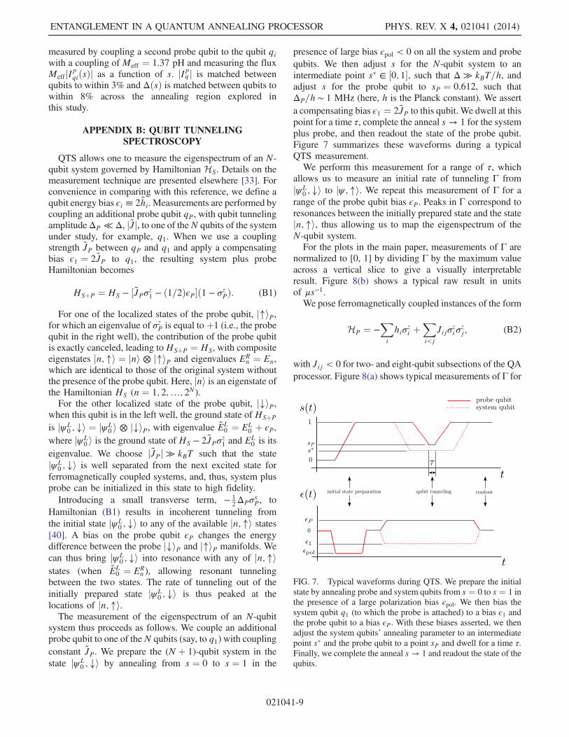
presence of large bias ϵpol < 0 on all the system and probequbits. We then adjust s for the N-qubit system to anintermediate point s� ∈ ½0; 1�, such that Δ ≫ kBT=h, andadjust s for the probe qubit to sP ¼ 0.612, such thatΔP=h ∼ 1 MHz (here, h is the Planck constant). We asserta compensating bias ϵ1 ¼ 2~JP to this qubit. We dwell at thispoint for a time τ, complete the anneal s → 1 for the systemplus probe, and then readout the state of the probe qubit.Figure 7 summarizes these waveforms during a typicalQTS measurement.We perform this measurement for a range of τ, which

allows us to measure an initial rate of tunneling Γ fromjψL

0 ;↓i to jψ ;↑i. We repeat this measurement of Γ for arange of the probe qubit bias ϵP. Peaks in Γ correspond toresonances between the initially prepared state and the statejn;↑i, thus allowing us to map the eigenspectrum of theN-qubit system.For the plots in the main paper, measurements of Γ are

normalized to [0, 1] by dividing Γ by the maximum valueacross a vertical slice to give a visually interpretableresult. Figure 8(b) shows a typical raw result in unitsof μs−1.We pose ferromagnetically coupled instances of the form

HP ¼ −Xi

hiσzi þ

Xi<j

Jijσziσ

zj; (B2)

with Jij < 0 for two- and eight-qubit subsections of the QAprocessor. Figure 8(a) shows typical measurements of Γ for

FIG. 7. Typical waveforms during QTS. We prepare the initialstate by annealing probe and system qubits from s ¼ 0 to s ¼ 1 inthe presence of a large polarization bias ϵpol. We then bias thesystem qubit q1 (to which the probe is attached) to a bias ϵ1 andthe probe qubit to a bias ϵP. With these biases asserted, we thenadjust the system qubits’ annealing parameter to an intermediatepoint s� and the probe qubit to a point sP and dwell for a time τ.Finally, we complete the anneal s → 1 and readout the state of thequbits.

ENTANGLEMENT IN A QUANTUM ANNEALING PROCESSOR PHYS. REV. X 4, 021041 (2014)

021041-9

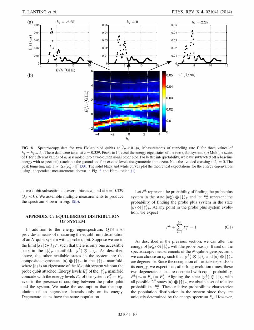
a two-qubit subsection at several biases hi and at s ¼ 0.339( ~JP < 0). We assemble multiple measurements to producethe spectrum shown in Fig. 8(b).

APPENDIX C: EQUILIBRIUM DISTRIBUTIONOF SYSTEM

In addition to the energy eigenspectrum, QTS alsoprovides a means of measuring the equilibrium distributionof an N-qubit system with a probe qubit. Suppose we are inthe limit j ~JPj ≫ kBT, such that there is only one accessiblestate in the j↓iP manifold: jψL

0 i ⊗ j↓iP. As describedabove, the other available states in the system are thecomposite eigenstates jni ⊗ j↑iP in the j↑iP manifold,where jni is an eigenstate of theN-qubit system without theprobe qubit attached. Energy levels ER

n of the j↑iP manifoldcoincide with the energy levels En of the system, ER

n ¼ En,even in the presence of coupling between the probe qubitand the system. We make the assumption that the pop-ulation of an eigenstate depends only on its energy.Degenerate states have the same population.

Let PL represent the probability of finding the probe plussystem in the state jψL

0 i ⊗ j↓iP and let PRn represent the

probability of finding the probe plus system in the statejni ⊗ j↑iP. At any point in the probe plus system evolu-tion, we expect

PL þX2Ni¼1

PRi ¼ 1: (C1)

As described in the previous section, we can alter theenergy of jψL

0 i ⊗ j↓iP with the probe bias ϵP. Based on thespectroscopic measurements of the N-qubit eigenspectrum,we can choose an ϵP such that jψL

0 i ⊗ j↓iP and jni ⊗ j↑iPare degenerate. Since the occupation of the state depends onits energy, we expect that, after long evolution times, thesetwo degenerate states are occupied with equal probability,PLðϵP ¼ EnÞ ¼ PR

n . Aligning the state jψL0 i ⊗ j↓iP with

all possible 2N states jni ⊗ j↑iP, we obtain a set of relativeprobabilities PR

n . These relative probabilities characterizethe population distribution in the system since they areuniquely determined by the energy spectrum En. However,

−4 −2 0 2 4

−2

0

2

4

6

0

0.01

0.02

0.03

0.04

0.05

0 5 10 150

0.01

0.02

0.03

0.04

0.05

0 5 10 150

0.01

0.02

0.03

0.04

0.05

0 5 10 150

0.01

0.02

0.03

0.04

0.05(a)

(b)

FIG. 8. Spectroscopy data for two FM-coupled qubits at ~JP < 0. (a) Measurements of tunneling rate Γ for three values ofh1 ¼ h2 ≡ hi. These data were taken at s ¼ 0.339. Peaks in Γ reveal the energy eigenstates of the two-qubit system. (b) Multiple scansof Γ for different values of hi assembled into a two-dimensional color plot. For better interpretability, we have subtracted off a baselineenergy with respect to (a) such that the ground and first excited levels are symmetric about zero. Note the avoided crossing at hi ¼ 0. Thepeak tunneling rate Γ ∼ jΔPhψL

0 jnij2 [33]. The solid black and white curves plot the theoretical expectations for the energy eigenvaluesusing independent measurements shown in Fig. 6 and Hamiltonian (1).

T. LANTING et al. PHYS. REV. X 4, 021041 (2014)

021041-10

as follows from Eq. (C1), the set PRn is not properly

normalized. The probability distribution of the systemitself is given by

PnðEnÞ ¼PRnP

2N

i¼1 PRi

; (C2)

whereP

2N

n¼1 Pn ¼ 1. At every eigenenergy, ϵP ¼ En, thedenominator of Eq. (C2) can be found from Eq. (C1), sothat the population distribution of the system Pn has theform

Pn ¼PRn

1 − PL ¼ PLðϵP ¼ EnÞ1 − PLðϵP ¼ EnÞ

: (C3)

Thus, the probability Pn to find the system of N qubits inthe state with energy En can be estimated by measuring PL

at ϵP ¼ En and using Eq. (C3).Measurements of PL proceed as they do for the spec-

troscopy measurements. The system plus probe is preparedin jψL

0 ;↓i. We then adjust ϵP ¼ En and an annealingparameter s for the N-qubit system to some intermediatepoint, and also sP ¼ 0.612 for the probe qubit, such thatΔP=h ∼ 1 MHz. We dwell at this point for a time τ ≫ 1=Γ,complete the anneal s → 1, and then readout the state of theprobe qubit. We typically investigate a range of τ to ensurethat we are in the long evolution time limit in which PL isindependent of τ. We use PL measured with τ ¼ 7041 μs toestimate P1 and P2. The Supplemental Material [34]contains typical data used for these estimates.

APPENDIX D: ENTANGLEMENT MEASURESAND WITNESSES

1. Definition of entanglement

A pure state jΨi of a system S consisting of two parts Aand B, S ¼ A∪B, is entangled [16] with relation to thisbipartition if the state jΨi cannot be represented as aproduct of states jΨAi and jΨBi describing the subsystemsA and B: jΨi ≠ jΨAi ⊗ jΨBi. An open quantum system ischaracterized by a density matrix ρ. An open system S isentangled [16] relative to the bipartition S ¼ A∪B if itsdensity matrix ρ cannot be written as a convex sum ofproduct states ρkA ⊗ ρkB, ρ ≠

Pkwkρ

kA ⊗ ρkB. Here, fρkAg

and fρkBg are sets of density matrices for the components Aand B, respectively; wk ≥ 0,

Pkwk ¼ 1. If there is no

bipartition for which the system is entangled, the state iscompletely separable or unentangled. If the system isentangled for all possible bipartitions, the state is globallyentangled.

2. Wχ : A susceptibility-based, ground-stateentanglement witness

For a bipartion of the system into two parts, A and B, wedefine a witness RAB as

RAB ¼ 1

4NAB

����Xi∈A

Xj∈B

~Jijχij

����; (D1)

where χij is a cross susceptibility, ~Jij ¼ EJij, and NAB is anumber of nonzero couplings, Jij ≠ 0, between qubits fromthe subset A and the subset B (see Ref. [35]). We note thatat low temperature, T ¼ 12.5 mK, the measured suscep-tibility χijðTÞ almost coincides with the ground-statesusceptibility χijðT ¼ 0Þ since contributions of excitedstates to χijðTÞ are proportional to their populations,Pn ≪ 1, for n > 1. We analyze a deviation of the mea-sured susceptibility from its ground-state value in theSupplemental Material [34]. To characterize globalentanglement in the system of N qubits, we introduce awitness Wχ ,

Wχ ¼ffiffiffiffiffiffiffiffiffiffiffiffiffiffiffiffiffiffiffiffiffiffiffiffiffiffiffiffiffiffiffiffiffiffiðQRABÞ1=Np

1þ ðQRABÞ1=Np

s; (D2)

which is given by a bounded geometrical mean of witnessesRAB calculated for all possible partitions of the wholesystem into two subsystems. Here, Np is a number of suchbipartitions, in particular, Np ¼ 127 for the eight-qubit ring.

3. Thermal density matrix ρ

Systems coupled to a thermal bath are in a mixed statewhen the energy gap between the ground and first excitedstates approaches kBT. Most mixed-state entanglementmeasures and witnesses require knowledge of the densitymatrix ρ. The density matrix can be measured usingquantum state tomography. However, this approach islimited to a small number of qubits [41]. As an alternateapproach, we consider an N-qubit system in a thermal(stationary) state [26]. The stationary system described byHamiltonian (1) can be characterized by a density matrixthat is diagonal in the energy basis, ρE ¼ diagfP1;P2;…; P2Ng. The off-diagonal elements of this matrixdisappear on a very short decoherence time scale (withina few nanoseconds) in the quantum annealing processoranalyzed in Ref. [6]. In thermal equilibrium, the occupationprobability Pμ ¼ e−Eμ=kBT=Z is the Boltzmann distributionover the eigenstates jμi with energies Eμ, such thatHjμi ¼ Eμjμi, T is temperature, and Z ¼ P

μe−Eμ=kBT

is the partition function. The density matrix ρ ¼PρM̄ N̄ jM̄ihN̄j in the computation basis jM̄i, where

ρM̄ N̄ ¼ PμPμhM̄jμihμjN̄i, is obtained from ρE by a unitary

transformation that depends on the parameters of theHamiltonian H. The parameters of Hamiltonian (1),

ENTANGLEMENT IN A QUANTUM ANNEALING PROCESSOR PHYS. REV. X 4, 021041 (2014)

021041-11

namely, the energy scale E, the qubit biases hi, tunnelingamplitudes Δ, coupling constants Jij, as well as proba-bilities Pμ, can be independently measured. This allows usto restore the density matrix ρ. We emphasize that thestationary-state entanglement, or thermal entanglement, isrobust and does not decay with time [26].

4. Concurrence C

For an open system described by a thermal densitymatrix ρ, concurrence C is defined as [16,18]

C ¼ maxf0;ffiffiffiffiffiλ4

p−

ffiffiffiffiffiλ3

p−

ffiffiffiffiffiλ2

p−

ffiffiffiffiffiλ1

pg; (D3)

where λ4 > λ3 > λ2 > λ1 are the roots of the matrix

R ¼ ρðσy1 ⊗ σy2Þρ�ðσy1 ⊗ σy2Þ; (D4)

fσxi ; σyi ; σzig are the Pauli matrices for the ith qubit, and ρ isthe density matrix of the system in the computation basis.An entanglement of formation Ef is another measure of

two-qubit entanglement. This measure is a monotonicfunction of concurrence C [16,18],

Ef ¼ F�1þ

ffiffiffiffiffiffiffiffiffiffiffiffiffi1 − C2

p

2

�; (D5)

where F ðxÞ ¼ −xlog2ðxÞ − ð1 − xÞlog2ð1 − xÞ is theentropy function.

5. Negativity N

Negativity is a measure that provides a sufficient, but notnecessary, condition for entanglement of an arbitrarynumber of qubits [36]. A nonzero value of negativitydetects entanglement. To calculate negativity, we find allbipartitions of the system. For two qubits, there is only onebipartition. An eight-qubit system can be bipartitioned into127 (¼ 8þ 28þ 56þ 35) possible combinations of twosubsystems, A and B. In the case when the state of thesystem is separable, its density matrix ρ should retain allproperties of the true density matrix after the partialtransposition of ρ with respect to the subsystem A or tothe subsystem B [16,36]. In particular, the partially trans-posed density matrix ρTA should not have negative eigen-values. The negativity, N ¼ ð1=2ÞPiðjλij − λiÞ, isproportional to the sum of all negative eigenvalues λi ofthe matrix ρTA , thus quantifying a degree of entangle-ment of the subsystem A and the subsystem B. For theeight-qubit system, we analyze negativities for all 127partitions, N 1=7, N 2=6, N 3=5, N 4=4, and calculate theirgeometrical average [42], or the global negativity, N ðρÞ ¼ðN 1=7N 2=6N 3=5N 4=4Þ1=127. Here, the negativity N 1=7 isequal to the product of 8 negativities for all possiblepartitions of the eight-qubit system into subsystems ofone and seven qubits, and so on. Nonzero values of the

global negativity mean that all possible subsystems of thewhole eight-qubit system are globally entangled. Note thatthe negativity of the maximally entangled GHZ state,N GHZ, is equal to 1=2.

6. Entanglement witness WAB

Consider Hamiltonian (1) with measured parameters.This Hamiltonian describes a transverse Ising model havingN qubits. The ground state jψ1i of this model is entangledwith respect to some bipartition A − B of the N-qubitsystem. We can form an operator jψ1ihψ1jTA, where TA is apartial transposition operator with respect to the A sub-system [16]. Let jϕi be the eigenstate of jψ1ihψ1jTA withthe most negative eigenvalue. We can form a new operatorWAB ¼ jϕihϕjTA . This operator can serve as an entangle-ment witness (it is trivially positive on all separablestates).Let ρðsÞ be the density matrix associated with the state of

the system at the annealing point s. If we have experimentalmeasurements of the occupation fraction of the ground stateand first excited state, P1ðsÞ � δP1 and P2ðsÞ � δP2,respectively, we can place a set of linear constraintson ρðsÞ:

Tr½ρðsÞjψ1ihψ1j� ≥ P1ðsÞ − δP1;

Tr½ρðsÞjψ1ihψ1j� ≤ P1ðsÞ þ δP1;

Tr½ρðsÞjψ2ihψ2j� ≥ P2ðsÞ − δP2;

Tr½ρðsÞjψ2ihψ2j� ≤ P2ðsÞ þ δP2:

We now search over all possible ρðsÞ that satisfy thelinear constraints provided by the experimental data. Thegoal is to maximize the witness Tr½WABρðsÞ� in order toestablish an upper limit for this quantity. Maximizing thisquantity can be cast as a semidefinite program [37], a classof convex optimization problems for which efficientalgorithms exist. When this upper limit is less than zero,entanglement is certified for the bipartition A − B.We test the robustness of this result with uncertainties in

the parameters of the Hamiltonian. To do this, we repeat theanalysis at several points during the QA algorithm whenadding random perturbations on the measured Hamiltonianthat correspond to the uncertainty on these measuredquantities. We sample 104 perturbed Hamiltonians and,for every perturbation, the optimization results inTr½WABρðsÞ� < 0.

[1] M. Mariantoni, H. Wang, T. Yamamoto, M. Neeley, R. C.Bialczak, Y. Chen, M. Lenander, E. Lucero, A. D.O’Connell, D. Sank, M. Weides, J. Wenner, Y. Yin, J.Zhao, A. N. Korotkov, A. N. Cleland, and J. M. Martinis,Implementing the Quantum von Neumann Architecture withSuperconducting Circuits, Science 334, 61 (2011).

T. LANTING et al. PHYS. REV. X 4, 021041 (2014)

021041-12

[2] E. Lucero, R. Barends, Y. Chen, J. Kelly, M. Mariantoni, A.Megrant, P. O’Malley, D. Sank, A. Vainsencher, J. Wenner,T. White, Y. Yin, A. N. Cleland, and J. M. Martinis,Computing Prime Factors with a Josephson Phase QubitQuantum Processor, Nat. Phys. 8, 719 (2012).

[3] M. D. Reed, L. DiCarlo, S. E. Nigg, L. Sun, L. Frunzio,S. M. Girvin, and R. J. Schoelkopf, Realization of Three-Qubit Quantum Error Correction with SuperconductingCircuits, Nature (London) 482, 382 (2012).

[4] A. G. Fowler, M. Mariantoni, J. M. Martinis, and A. N.Cleland, Surface Codes: Towards Practical Large-ScaleQuantum Computation, Phys. Rev. A 86, 032324(2012).

[5] T. S. Metodi, D. D. Thaker, and A.W. Cross, Proceedings ofthe 38th Annual IEEE/ACM International Symposium onMicroarchitecture (MICRO-38), 2005 (IEEE, New York,2005).

[6] M.W. Johnson et al., Quantum Annealing with Manufac-tured Spins, Nature (London) 473, 194 (2011).

[7] N. G. Dickson et al., Thermally Assisted QuantumAnnealing of a 16-Qubit Problem, Nat. Commun. 4,1903 (2013).

[8] R. Harris et al., Experimental Investigation of an Eight-Qubit Unit Cell in a Superconducting Optimization Proc-essor, Phys. Rev. B 82, 024511 (2010).

[9] R. Blatt and D. Wineland, Entangled States of TrappedAtomic Ions, Nature (London) 453, 1008 (2008).

[10] T. Monz, P. Schindler, J. T. Barreiro, M. Chwalla, D. Nigg,W. A. Coish, M. Harlander, W. Hänsel, M. Hennrich, and R.Blatt, 14-Qubit Entanglement: Creation and Coherence,Phys. Rev. Lett. 106, 130506 (2011).

[11] M. Ansmann, H. Wang, R. C. Bialczak, M. Hofheinz, E.Lucero, M. Neeley, A. D. O’Connell, D. Sank, M. Weides, J.Wenner, A. N. Cleland, and J. M. Martinis, Violation ofBell’s Inequality in Josephson Phase Qubits, Nature (Lon-don) 461, 504 (2009).

[12] M. Neeley, R. C. Bialczak, M. Lenander, E. Lucero, M.Mariantoni, A. D. O’Connell, D. Sank, H. Wang, M.Weides, J. Wenner, Y. Yin, T. Yamamoto, A. N. Cleland,and J. M. Martinis, Generation of Three-Qubit EntangledStates Using Superconducting Phase Qubits, Nature(London) 467, 570 (2010).

[13] L. DiCarlo, M. D. Reed, L. Sun, B. R. Johnson, J. M. Chow,J. M. Gambetta, L. Frunzio, S. M. Girvin, M. H. Devoret,and R. J. Schoelkopf, Preparation and Measurement ofThree-Qubit Entanglement in a Superconducting Circuit,Nature (London) 467, 574 (2010).

[14] A. J. Berkley, H. Xu, R. C. Ramos, M. A. Gubrud, F. W.Strauch, P. R. Johnson, J. R. Anderson, A. J. Dragt, C. J.Lobb, and F. C. Wellstood, Entangled MacroscopicQuantum States in Two Superconducting Qubits, Science300, 1548 (2003).

[15] G. Vidal, Efficient Classical Simulation of Slightly En-tangled Quantum Computations, Phys. Rev. Lett. 91,147902 (2003).

[16] O. Gühne and G. Tóth, Entanglement Detection, Phys. Rep.474, 1 (2009).

[17] D. Greenberger, M. Horne, A. Shimony, and A. Zeilinger,Bells Theorem without Inequalities, Am. J. Phys. 58, 1131(1990).

[18] W. K. Wootters, Entanglement of Formation of anArbitrary State of Two Qubits, Phys. Rev. Lett. 80, 2245(1998).

[19] A. B. Finnila, M. A. Gomez, C. Sebenik, C. Stenson, andJ. D. Doll, Quantum Annealing: A New Method for Mini-mizing Multidimensional Functions, Chem. Phys. Lett. 219,343 (1994).

[20] T. Kadowaki and H. Nishimori, Quantum Annealing in theTransverse Ising Model, Phys. Rev. E 58, 5355 (1998).

[21] E. Farhi, J. Goldstone, S. Gutmann, J. Lapan, A. Lundgren,and D. Preda, A Quantum Adiabatic Evolution AlgorithmApplied to Random Instances of an NP-Complete Problem,Science 292, 472 (2001).

[22] G. E. Santoro, R. Martonak, E. Tosatti, and R. Car, Theoryof Quantum Annealing of an Ising Spin Glass, Science 295,2427 (2002).

[23] A. Perdomo-Ortiz, N. Dickson, M. Drew-Brook, G. Rose,and A. Aspuru-Guzik, Finding Low-Energy Conformationsof Lattice Protein Models by Quantum Annealing, Sci. Rep.2, 571 (2012).

[24] S. Boixo, T. Albash, F. M. Spedalieri, N. Chancellor, andD. A. Lidar, Experimental Signature of ProgrammableQuantum Annealing, Nat. Commun. 4, 2067 (2013).

[25] R. Harris, T. Lanting, A. J. Berkley, J. Johansson, M.W.Johnson, P. Bunyk, E. Ladizinsky, N. Ladizinsky, T. Oh, andS. Han, A Compound Josephson Junction Coupler for FluxQubits with Minimal Cross Talk, Phys. Rev. B 80, 052506(2009).

[26] L. Amico, R. Fazio, A. Osterloch, and V. Vedral, Entangle-ment in Many-Body Systems, Rev. Mod. Phys. 80, 517(2008).

[27] X. Wang, Thermal and Ground-State Entanglement inHeisenberg XX Qubit Rings, Phys. Rev. A 66, 034302(2002).

[28] S. Ghosh, T. F. Rosenbaum, G. Aeppli, and S. N. Copper-smith, Entangled Quantum State of Magnetic Dipoles,Nature (London) 425, 48 (2003).

[29] T. Vértesi and E. Bene, Thermal Entanglement in theNanotubular System Na2V3O7, Phys. Rev. B 73, 134404(2006).

[30] C. Brukner, V. Vedral, and A. Zeilinger, Crucial Role ofQuantum Entanglement in Bulk Properties of Solids, Phys.Rev. A 73, 012110 (2006).

[31] T. G. Rappoport, L. Ghivelder, J. C. Fernandes, R. B.Guimaraes, and M. A. Continentino, Experimental Obser-vation of Quantum Entanglement in Low-DimensionalSystems, Phys. Rev. B 75, 054422 (2007).

[32] N. B. Christensen, H. M. Ronnow, D. F. McMorrow, A.Harrison, T. G. Perring, M. Enderle, R. Coldea, L. P.Regnault, and G. Aeppli, Quantum Dynamics and Entan-glement of Spins on a Square Lattice, Proc. Natl. Acad. Sci.U.S.A. 104, 15 264 (2007).

[33] A. J. Berkley, A. J. Przybysz, T. Lanting, R. Harris, N.Dickson, F. Altomare, M. H. Amin, P. Bunyk, C. Enderud,E. Hoskinson, M.W. Johnson, E. Ladizinsky, R. Neufeld, C.Rich, A. Y. Smirnov, E. Tolkacheva, S. Uchaikin, and A. B.Wilson, Tunneling Spectroscopy Using a Probe Qubit,Phys. Rev. B 87, 020502 (2013).

[34] See Supplemental Material at http://link.aps.org/supplemental/10.1103/PhysRevX.4.021041 includes

ENTANGLEMENT IN A QUANTUM ANNEALING PROCESSOR PHYS. REV. X 4, 021041 (2014)

021041-13

additional information on susceptibility and spectroscopymeasurements, additional detail on data analysis, and adiscussion of the susceptiblity-based witness at finitetemperature.

[35] A. Yu. Smirnov and M. H. Amin, Ground-State Entangle-ment in Coupled Qubits, Phys. Rev. A 88, 022329(2013).

[36] G. Vidal and R. F. Werner, A Computable Measure ofEntanglement, Phys. Rev. A 65, 032314 (2002).

[37] F. M. Spedalieri, Detecting Entanglement with Partial StateInformation, Phys. Rev. A 86, 062311 (2012).

[38] R. Harris, J. Johansson, A. J. Berkley, M.W. Johnson, T.Lanting, S. Han, P. Bunyk, E. Ladizinsky, T. Oh, I.Perminov, E. Tolkacheva, S. Uchaikin, E. M. Chapple, C.Enderud, C. Rich, M. Thom, J. Wang, B. Wilson, and G.Rose, Experimental Demonstration of a Robust andScalable Flux Qubit, Phys. Rev. B 81, 134510(2010).

[39] J. Johansson, M. H. S. Amin, A. J. Berkley, P. Bunyk,V. Choi, R. Harris, M.W. Johnson, T. M. Lanting,S. Lloyd, and G. Rose, Landau-Zener Transitions in aSuperconducting Flux Qubit, Phys. Rev. B 80, 012507(2009).

[40] R. Harris, M.W. Johnson, S. Han, A. J. Berkley, J. Johans-son, P. Bunyk, E. Ladizinsky, S. Govorkov, M. C. Thom, S.Uchaikin, B. Bumble, A. Fung, A. Kaul, A. Kleinsasser, M.H. S. Amin, and D. V. Averin, Probing Noise in Flux Qubitsvia Macroscopic Resonant Tunneling, Phys. Rev. Lett. 101,117003 (2008).

[41] M. P. da Silva, O. Landon-Cardinal, and D. Poulin,Practical Characterization of Quantum Devices withoutTomography, Phys. Rev. Lett. 107, 210404 (2011).

[42] P. J. Love, A. M. van den Brink, A. Yu. Smirnov, M. H. S.Amin, M. Grajcar, E. Il’ichev, A. Izmalkov, and A. M.Zagoskin, A Characterization of Global Entanglement,Quantum Inf. Process. 6, 187 (2007).

T. LANTING et al. PHYS. REV. X 4, 021041 (2014)

021041-14