Earth Planets Space, 61, 397–410, 2009

Equatorial GPS ionospheric scintillations over Kototabang, Indonesiaand their relation to atmospheric waves from below

Tadahiko Ogawa1∗, Yasunobu Miyoshi2, Yuichi Otsuka1, Takuji Nakamura3, and Kazuo Shiokawa1

1Solar-Terrestrial Environment Laboratory, Nagoya University, Toyokawa, Aichi 442-8507, Japan2Department of Earth and Planetary Sciences, Kyushu University, Fukuoka 812-8581, Japan

3Research Institute for Sustainable Humanosphere, Kyoto University, Uji, Kyoto 611-0011, Japan

(Received October 5, 2007; Revised January 25, 2008; Accepted March 12, 2008; Online published May 14, 2009)

Using Global Positioning System (GPS) satellites, we have been conducting equatorial ionospheric scintillationobservations at Kototabang, Indonesia since January 2003. Scintillations caused by equatorial plasma bubblesappear between 2000 and 0100 LT in equinoctial months with a seasonal asymmetry, and their activity decreaseswith decreasing solar activity. A comparison between scintillation index (S4) and Earth’s brightness temperature(Tbb) variations suggests that the scintillation activity can be related to tropospheric disturbances over the IndianOcean to the west of Kototabang. To understand better the reasons of day-to-day variability of S4, we analyze S4,Tbb and lower thermospheric neutral wind (u′2) data. The results show that S4 fluctuates with periods of about2.5, 5, 8, 14 and 25 days, possibly due to atmospheric waves from below and that similar periods are also foundin the Tbb and u′2 variations. Using a general circulation model, we made numerical simulations to determinethe behavior of neutral wind in the equatorial thermosphere. The results indicate the following: (1) 2- to 20-daywaves dissipate rapidly above about an altitude of 125 km, and 0.5- to 3-hour waves become predominant above100 km, (2) zonal winds above 200 km altitude are, on the whole, eastward during sunset-sunrise, (3) zonal windpatterns due to short-period (1–4 h) atmospheric gravity waves (AGWs) above 120 km altitude change day by day,exhibit wavy structures with scale lengths of about 30–1000 km and, as a whole, move eastward at about 100−1

while changing patterns over time. These simulations suggest that the Rayleigh-Taylor instability responsiblefor plasma bubble generation can be seeded by AGWs with short periods of about 0.5–3 h, and that backgroundconditions necessary for this instability are modulated by planetary-scale atmospheric waves propagating up toan altitude of about 120 km from below.Key words: Equatorial ionosphere, GPS scintillation, plasma bubble, atmospheric wave, tropospheric distur-bance.

1. IntroductionOne of the plasma disturbances peculiar to the nighttime

equatorial ionosphere concerns the plasma bubbles that aregenerated in the bottomside of the F region near sunsetthrough the Rayleigh-Taylor (RT) plasma instability mech-anism. Bubbles are recognized as spread echoes on iono-grams (equatorial spread-F), and are accompanied by HF-VHF radar echoes and ionospheric scintillations of satellitesignals. Giant geomagnetic-conjugate bubbles extending upto 1800 km altitude over the geomagnetic equator have of-ten been detected simultaneously with all-sky imagers atmidlatitude in Japan and Australia (Otsuka et al., 2002; Sh-iokawa et al., 2004; Ogawa et al., 2005). Although bubblecharacteristics and fundamental physical processes gener-ating bubbles have been well studied, many questions stillremain to be answered for a full understanding of the elec-trodynamics related to bubbles and spread-F (e.g., Abdu,

∗Now at National Institute of Information and Communications Tech-nology, Koganei, Tokyo 184-8795, Japan.

Copyright c© The Society of Geomagnetism and Earth, Planetary and Space Sci-ences (SGEPSS); The Seismological Society of Japan; The Volcanological Societyof Japan; The Geodetic Society of Japan; The Japanese Society for Planetary Sci-ences; TERRAPUB.

2001). The issues that we are concerned with in this pa-per are the day-to-day variability of bubble occurrences andseeding processes of plasma perturbations that ultimatelydevelop into bubbles through the RT instability.Plasma bubbles are usually accompanied by field-aligned

irregularities (FAIs) with various spatial scales. FAIs on thescale of a few meters cause coherent VHF radar backscat-ter (e.g., Woodman and LaHoz, 1976; Fukao et al., 2004),and those on a scale of a few hundred meter induce iono-spheric scintillations when a Global Positioning System(GPS) radio wave penetrates into the horizontally movingFAI region (Beach and Kintner, 1999). Basu et al. (1983)observed 257-MHz and 1.54-GHz scintillations associatedwith plasma depletions that were detected with an in situprobe. Using the 47-MHz EAR radar and a 630-nm all-skyimager at Kototabang, Otsuka et al. (2004) found that 3.2-m scale FAIs were confined within plasma bubbles. Theseobservations indicate a GPS scintillation technique to bevery useful to monitor continuously plasma bubble occur-rences throughout day, season and year. GPS scintillationsare caused by FAIs with a spatial scale of about 350 m (firstFresnel size) within and around bubbles.Atmospheric gravity waves (AGWs) propagating in the

equatorial thermosphere can seed plasma bubbles (e.g. Lin

397

398 T. OGAWA et al.: IONOSPHERIC SCINTILLATIONS AND ATMOSPHERIC WAVES

J F M A M J J A S O N D

J F M A M J J A S O N D

Month

S4

Kototabang, Sumatra (0.2 S, 100.3 E; dip. lat.=10.4 S)o

0 0.2 0.4 0.6 1.0

Lo

cal T

ime

(h

ou

rs)

20

22

0

2

o o

Elevation Angle 30o

0.8

2003

2004

2005

2006

2007

20

22

0

2

20

22

0

2

20

22

0

2

20

22

0

2

20

22

0

2

20

22

0

2

20

22

0

2

20

22

0

2

20

22

0

2

No Data

Fig. 1. Day-local time variations in the GPS scintillation index S4 at Kototabang during January 2003–June 2007. S4 values less than about 0.2 are dueto background noise. Black portions represent no data due to instrumental problems.

et al., 2005) and cause a sinusoidal oscillation of the al-titude of the bottomside F layer (Kelley et al., 1981) andwavy ion density structures with east-west wavelengths of150–800 km in the bottomside F layer (Singh et al., 1997).Tsunoda (2005) stressed that development of a large-scale(∼400 km) wavy structure was necessary for spread-F oc-currence and to explain day-to-day variability of spread-F.Ogawa et al. (2005) found wavy plasma structures withscales of a few hundred to 1000 km within the northernand southern equatorial anomaly crests. Planetary waves(PWs) with periods longer than 2 days are known to modu-late the equatorial mesosphere and ionosphere (Takahashiet al., 2005) and occurrences of the evening prereversalenhancement of the equatorial electric field and spread-F(Abdu et al., 2006a). Thus, the role of AGWs and PWs,probably propagating from below, cannot be disregardedwhen trying to understand the seeding and modulation pro-cesses of plasma bubbles and also vertical coupling in theatmosphere-ionosphere system (Lastovicka, 2006).We have been monitoring GPS ionospheric scintilla-

tions at Kototabang, West Sumatra in Indonesia (0.20◦S,100.32◦E; geomagnetic latitude � dip latitude 10.36◦S)

near the geographic equator since January 2003. Usingthe data from 2003 and 2004, Ogawa et al. (2006) pre-sented characteristics of equatorial ionospheric scintilla-tions over Kototabang. They also compared scintillationactivity with the Earth’s black body temperature (a measureof tropospheric disturbance) in order to investigate possibledynamical coupling between the ionosphere/thermosphereand troposphere over the equator. The results suggested thatsome correlations can exist between the scintillation (bub-ble) occurrence and tropospheric disturbance over the In-dian Ocean.In this paper we show the scintillation characteristics dur-

ing January 2003–June 2007 (during the declining phaseof 11-year solar cycle) and make a wavelet analysis ofscintillation, mesospheric/lower thermospheric wind andblack body temperature data to investigate modulations ofthese parameters due to long-period (≥2 days) atmosphericwaves. Further, to know how PWs and AGWs behavein the equatorial mesosphere and thermosphere/ionosphere,we make numerical simulations of neutral winds at altitudesbetween the ground and about 500 km, using a general cir-culation model with high spatial resolution.

T. OGAWA et al.: IONOSPHERIC SCINTILLATIONS AND ATMOSPHERIC WAVES 399

East Longitude Local Time

60

100

70

90

110

120

2003

Day

of

20

03

20 22 070 90 100 2

220 240 260 300 K

80

280

80

60

100

70

90

110

120

80

Tbb (2 S-2 N, 0-24 UT)o o Kototabang S4

Kototabang

0 0.2 0.4 0.6 1.00.8

S4

0.2

0.6

0.4

Fig. 2. Daily variations of black body temperature Tbb, averaged over 2◦S–2◦N and 0000–2400 UT, and GPS scintillation index S4 during March 1 (day60)–April 30 (day 120), 2003. Daily variation in S4 averaged over 1900–2300 LT is also plotted by white curve. Vertical line in Tbb plot indicates thelongitude of Kototabang (100.32◦E). Black portions in S4 plot denote the absence of observations due to instrumental problems.

2. Observations and Analysis2.1 GPS scintillation observationsIn January 2003, we started to monitor ionospheric scin-

tillations at Kototabang by means of three spaced 1.5754-GHz GPS receivers located with baseline distances of 116,127 and 152 m. Our aim is to measure the drift velocity ofFAIs (Ogawa et al., 2006; Otsuka et al., 2006). The scintil-lation magnitude is represented by the index S4 that is de-fined as the normalized standard deviation of signal inten-sity, i.e. S2

4 = (〈I 2〉 − 〈I 〉2) /〈I 〉2, where I is the signal in-tensity, and the angle brackets denote the ensemble averageof the enclosed quantity. S4 was calculated every 10 min byusing data from one of the receivers that provide signal in-tensity with a sampling rate of 20 Hz (50 ms). When signalsfrom multiple GPS satellites were simultaneously received,the highest S4 of all the S4 values was selected. The S4 datawith satellite elevation angles ≥30◦ were used to determinethe scintillation occurrence within the circular area, cover-ing the geomagnetic latitudes between 4◦ and 13◦S, with aradius of 520 km at 300 km altitude over Kototabang (seeFig. 3).Figure 1 shows S4 variations from January 2003 to June

2007 in day-local time coordinates. The S4 values lessthan about 0.2 originate from radio interference, receivernoise, etc. and, therefore, should be disregarded. Thevertical black portions represent the absence of data dueto instrumental problems, which happened sporadically.Such problems, however, do not detect from the follow-ing discussion on the scintillation activity characteristics.Figure 1 indicates the following: (1) scintillation activ-ity clearly decreases with decreasing solar activity from2003 to 2007; (2) scintillations appear predominantly inequinoctial months, i.e. in March–April and September–October, and mostly between near local sunset (∼2000 LT;LT=UT+ 7 h at Kototabang) and 0100 LT in March–April

and between 2000 and 2300 LT in September–October; (3)scintillation occurrences show clear day-to-day variabilityand are more frequent in March–April than September–October. Plasma bubbles imaged by an all-sky camera areknown to appear between sunset and later hours after mid-night, while the GPS scintillations disappear at around mid-night, as shown in Fig. 1: the latter fact means that the 350-km scale electron density irregularities causing the scintilla-tions disappear after midnight. Thus, Fig. 1 can be regardedas a proxy of the plasma bubble occurrences before mid-night over Kototabang. Since the bubbles near Kototabangare generated near the sunset terminator and then move east-ward at about 100−1 (Yokoyama et al., 2004; Fukao et al.,2006; Otsuka et al., 2006), the scintillations at earlier lo-cal times are believed to be generated at locations closer toKototabang.2.2 Comparison between scintillations and tropo-

spheric disturbancesA number of physical processes are responsible for caus-

ing the GPS scintillation activity shown in Fig. 1. One ofthese may be tropospheric disturbances in the equatorial re-gion, which launch atmospheric waves that propagate up-ward toward the ionosphere. In this paper, as a measure oftropospheric disturbances, we use black body temperature(Tbb) (often called the “cloud-top temperature”) of the Earthinferred from Outgoing Long wave Radiation (OLR) datathat were continuously monitored at 1-h intervals from geo-stationary meteorological satellites (GMS-5 before 21 May2003 and GOES-9 after 22 May 2003). In general, lower(higher) Tbb indicates the cloud top altitude to be higher(lower) because of more (less) active tropospheric convec-tion. It has been pointed out that AGWs inducing iono-spheric plasma disturbances may be launched upward fromactive convection regions in the troposphere (e.g., Rottger,1977, 1981; Hocke and Tsuda, 2001; Tsuda and Hocke,

400 T. OGAWA et al.: IONOSPHERIC SCINTILLATIONS AND ATMOSPHERIC WAVES

90 100 90 100

20

0

10

20

0

La

titu

de 10

20

0

10

East Longitude90 100

20

0

La

titu

de

10

20

0

La

titu

de

10

20

0

10

Correlation Between Tbb and S4 March 1 - April 30, 2003

S4 Deviation: 2100 - 2300 LT

East Longitude East Longitude

90 100 90 100

90 100

80 80

80

80 80 80

Tbb:1100 UT

Tbb:1400 UT

Tbb:1700 UT

Tbb:1300 UT

Tbb:1600 UT

Tbb:1200 UT

Tbb:1500 UT

Tbb:1800 UT

0 0.40.2-0.4 -0.2

Cross Correlation Coefficient

Fig. 3. Time variation of cross-correlation coefficients between S4 and Tbb. In calculating coefficients, S4 deviated from the average over 2100–2300 LTand March 1–April 30, 2003, and hourly Tbb deviated from the average over March 1–April 30, 2003 are used. GPS scintillation data were obtainedwithin the circular area with a radius of 520 km at 300 km altitude over Kototabang (�), which corresponds to a satellite elevation angle of ≥30◦, areused to calculate S4. The geomagnetic equator at about 9◦N is indicated by the horizontal red line.

2004). Tsuda et al. (2000) and Tsuda and Hocke (2004)showed that AGW energy in the stratosphere inferred fromGPS/Meteorology data is enhanced, in particular, over In-donesia where Tbb is low (cold).As an example, Fig. 2 shows daily variations of S4 at Ko-

totabang and Tbb during March 1 (day 60)–April 30 (day120), 2003. Note that a similar figure also appears in Fig. 6of Ogawa et al. (2006). The Tbb plot covers longitudes be-tween 70◦ and 102◦E (Kototabang longitude= 100.32◦E).The Tbb values averaged over 2◦S–2◦N and 0000–2400 UTare plotted in the figure. In the Tbb plot the cloud clus-ters with low temperature move eastward, and the organizedtemperature structures over the Indian Ocean are often dis-turbed at around 100◦E near Kototabang due to high moun-tains in Sumatra. It can be observed that when the scintil-lations occur between 2000 and 0000 LT, the Tbb values arehigher than, say, 270 K somewhere between 70◦ and 95◦E:for example, the scintillations on days 67–76, 81, 95–99 and102–104 are correlated to high Tbb at 80◦–96◦E. However,

this is not always true for other scintillation events; the Tbb

values for the scintillations on days 83–84 and 119 are loweverywhere, and those for the scintillations on days 92–93are high at 70◦–82◦E but low at 82◦–98◦E.To know quantitative relations between S4 and Tbb, cross-

correlation coefficients (R) between the two parameterswere calculated. For these calculations we used the S4values deviated from the average over 2100–2300 LT andMarch 1–April 30, 2003, and the hourly Tbb values deviatedfrom the average over the same days. The results are dis-played in Fig. 3. As described above, the scintillation dataobtained within the circular area with a radius of 520 km at300 km altitude over Kototabang, which corresponds to asatellite elevation angle of ≥30◦, were adopted to calculateS4. The high positive (red) and negative (blue) R values ex-ceeding ±0.45 appear predominantly in the 1400–1600 UTpanels. A high positive R area exists at latitudes of 0◦–10◦Nand longitudes of 75◦–82◦E, while high negative R areas oc-cur between 80◦ and 100◦E to the north and the south of the

T. OGAWA et al.: IONOSPHERIC SCINTILLATIONS AND ATMOSPHERIC WAVES 401

Jan 2003 - Jul 2005

200 400 600100 300 500 700 9001DayJan 1

0.0

0.1

2

4

8

16

32

64

Pe

rio

d (

day

s)

Jul 102003 2004 2005

SC0.2

S4

Dev

iatio

n (

18 -

02

LT)

800

90

%

90

%

90

%

2.5

5

10

20

(x10

)

-3P

owe

r

(b)

(a)

(c)

Lo

cal T

ime

(h

ou

rs)

20

22

0

2200 400 600100 300 500 700 9001 800

S4

0

0.2

0.4

0.6

0.8

1.0

Total Day

20042003 2005

Fig. 4. (a) Day-local time variations of S4 during January 2003–July 2005 (see Fig. 1). (b) Daily variation of S4 deviated from average over1800–0200 LT and 920 days is plotted. Geomagnetic storm commencement (SC) is marked by arrow. (c) Wavelet power spectra of S4 variationshown in (b). 90% confidence level is shown by thick solid curve. Spectra within cross-hatched areas are unreliable.

high positive R area. Note that R is positive when both S4and Tbb are high or low, while it is negative when one ishigh and the other is low, which means that for high (low)S4, Tbb at the red areas are high (low), and Tbb at the blueareas are low (high). One of the possible reasons why thered and blue areas are clearly separated in latitude is as fol-lows: when the tropospheric convection is active (accord-ingly, low Tbb) at latitudes of 0◦–10◦N and longitudes of75◦–82◦E, the convection at 80◦–100◦E to the north and thesouth of 0◦–10◦N becomes inactive (high Tbb) because ofmeridional circulation from the active region to the inactiveregions. In any case, Fig. 3 suggests that the scintillation oc-currences over Kototabang before midnight can be relatedto the tropospheric disturbances (high and low Tbb) mainlyover the Indian Ocean to the west of Kototabang.2.3 Wavelet analysis of S4, Tbb and lower thermo-

sphere windTo determine the spectral components of the Tbb and S4

variations, we made a wavelet analysis of both parameters.Figure 4(a) shows day-local time variations of S4 duringJanuary 2003–July 2005 (see Fig. 1). The daily variation ofS4 deviated from average over 1800–0200 LT and 920 daysis displayed in Fig. 4(b), where geomagnetic storm com-mencement (SC) is marked by a vertical arrow. Althoughsome geomagnetic storms might induce GPS scintillations,we think that as shown in Fig. 4(b), the association betweenthe SC and scintillation occurrences in equinoctial monthsis poor. Figure 4(c) shows wavelet power spectra of the S4

variation (Fig. 4(b)) in day-period coordinates. A 90% con-fidence level is shown by the thick solid curve. The spectrawithin the cross-hatched areas are unreliable because of aninsufficient amount of the data. Some spectral peaks hav-ing periods between 2 and 30 days can be clearly seen inequinoctial months in which the scintillations are highly ac-tivated. The S4 spectra in equinoctial months in 2003 and2004 are enlarged in Fig. 5. InMarch–April 2003 (Fig. 5(a))some spectral peaks appear between the 2- and 15-day pe-riod and a peak at around 24-day period. The spectral peaksbetween the 2- and 10-day period and at around the 24-dayperiod are observed in March–April 2004 (Fig. 5(c)). Sim-ilar spectral peaks with weak power are also discerned inSeptember–October 2003 (Fig. 5(b)) and 2004 (Fig. 5(d)).Next we compare wavelet periods among S4, neutral

winds in the lower thermosphere and Tbb. The neutral windswere measured with a meteor radar at Kototabang. In brief,this radar is operated at 37.7 MHz with an output power of12 kW and estimates horizontal wind velocities at an alti-tudes of 80–102 km with time and altitude resolutions of 1 hand 2 km, respectively (Sridharan et al., 2006). Only zonalwinds are examined in this paper. First, using hourly zonalwind data at a certain altitude, deviations from the 1-dayaverage were obtained. Second, the deviations were pro-cessed to calculate a time variation of the wind component(u′) with certain periods (2–8 and 2–24 h in our case). Fi-nally, the squared wind component (u′2) was averaged over1 day to know the daily variance (u′2) of the zonal wind.

402 T. OGAWA et al.: IONOSPHERIC SCINTILLATIONS AND ATMOSPHERIC WAVES

2

4

8

16

32

Pe

rio

d (

day

s)

60 80 100 120 140

2

4

8

16

32

Pe

rio

d (

day

s)

2

4

8

16

32

2

4

8

16

3240 220 260 280 300 320240

60 80 100 120 14040 220 260 280 300 320240

90%

90%

90

%

90%

90%

90%

90

%

Feb 1 - May 30, 2003

Jan 30 - May 29, 2004

Aug 8 - Nov 26, 2003

Aug 7 - Nov 25, 2004

S4 Wavelet Spectrum

Day

Day

Day

Day

2

4

16

8

(x10

)

-3P

ow

er

(a) (b)

(c) (d)

S4(18-02 LT)

Fig. 5. Wavelet power spectra of S4 in four seasons. (a) February 1–May 30, 2003, (b) August 8–November 26, 2003, (c) January 30–May 29, 2004and (d) August 7–November 25, 2004. 90% confidence level is shown by thick solid curve.

Jan 30 - May 30, 2003

Apr MayFeb MarDay40 60 100 120 140

2

4

16

32

2

4

16

32

40 60 100 120 140

2

4

16

32

Pe

rio

d (

day

s)

8

' 2

S4(18-02 LT)

U (2- h) 92 km8

8

80

80

2

4

16

322

4

16

32

8

8

Jan 30 - May 30, 200340 60 100 120 14080

8

90%

90%

90%

90%

90%

2

4

16

8

2

4

1

8

2

4

16

8

2

4

16

8

2

4

1

8

(x1

0

)-3

Po

we

r(x

10

)

5P

ow

er

90%

90%

90%

90%

90%

90%

90%

2

4

16

32

2

4

16

32

2

4

16

32

Pe

rio

d (

day

s)

8

8

8

2

4

16

322

4

16

32

8

8

S4(18-02 LT)

0N,80E

2

4

16

8

2.5

5

10

20

Apr MayFeb MarDay40 60 100 120 14080

Tbb

Tbb

Tbb

Tbb

0N,85E

0N,90E

0N,95E

(b)(a)

90%

(x1

0

)5

Po

we

r(x

10

)

5P

ow

er

(x1

0

)5

Po

we

r

(x1

0

)5

Po

we

r(x

10

)

-3P

ow

er

' 2U (2-24h) 92 km

' 2U (2- h) 86 km

8

' 2U (2-24h) 86 km

Fig. 6. Wavelet power spectra during January 30–May 30, 2003. (a) S4 and u′2 with periods of 2–8 and 2–24 h at altitudes of 92 and 86 km. (b) S4 andTbb at (0◦N, 80◦E), (0◦N, 85◦E), (0◦N, 90◦E), and (0◦N, 95◦E). 90% confidence level is shown by the thick solid curve.

Figure 6(a) shows wavelet spectra of S4 and u′2 with peri-ods of 2–8 and 2–24 h at altitudes of 92 and 86 km duringJanuary 30–May 30, 2003. Note that no data of S4 and u′2were obtained before day 60 and after day 120, respectively.

During days 60–120, the spectral peaks existing betweenthe 2- and 15-day period and at around the 24-day periodin S4 are also discerned in the u′2 spectra: in detail, the S4peaks between the 2- and 24-day period during days 65–90

T. OGAWA et al.: IONOSPHERIC SCINTILLATIONS AND ATMOSPHERIC WAVES 403

0

2

1

2

0

1

(x1

0

)3

Tb

b P

SD

S4

PS

D

Period (days)2 4 16 323 6 12 24

0

2

4

6

U

P

SD

'2

2

0

1

S4

PS

D

8

2 4 16 323 6 12 248

(b)

(x1

0

)5

(x1

0

)-2

(x1

0

)-2

S4

95%

95%

S4

(a) S4 (2003 Days: 60-120)

86 km : 2-24 h92 km : 2-24 h

2-8 h2-8 h

U (2003 Days: 30-120) ' 2

S4 (2003 Days: 60-120)Tbb (2003 Days: 30-150) 0N : 80E 85E

90E 95E

3

Fig. 7. Periodgrams of S4, Tbb and u′2 with periods of 2–8 and 2–24 h at altitudes of 92 and 86 km for wavelet power spectra shown in Fig. 6. 95%confidence level of each power spectral density (PSD) is shown by thin solid curve.

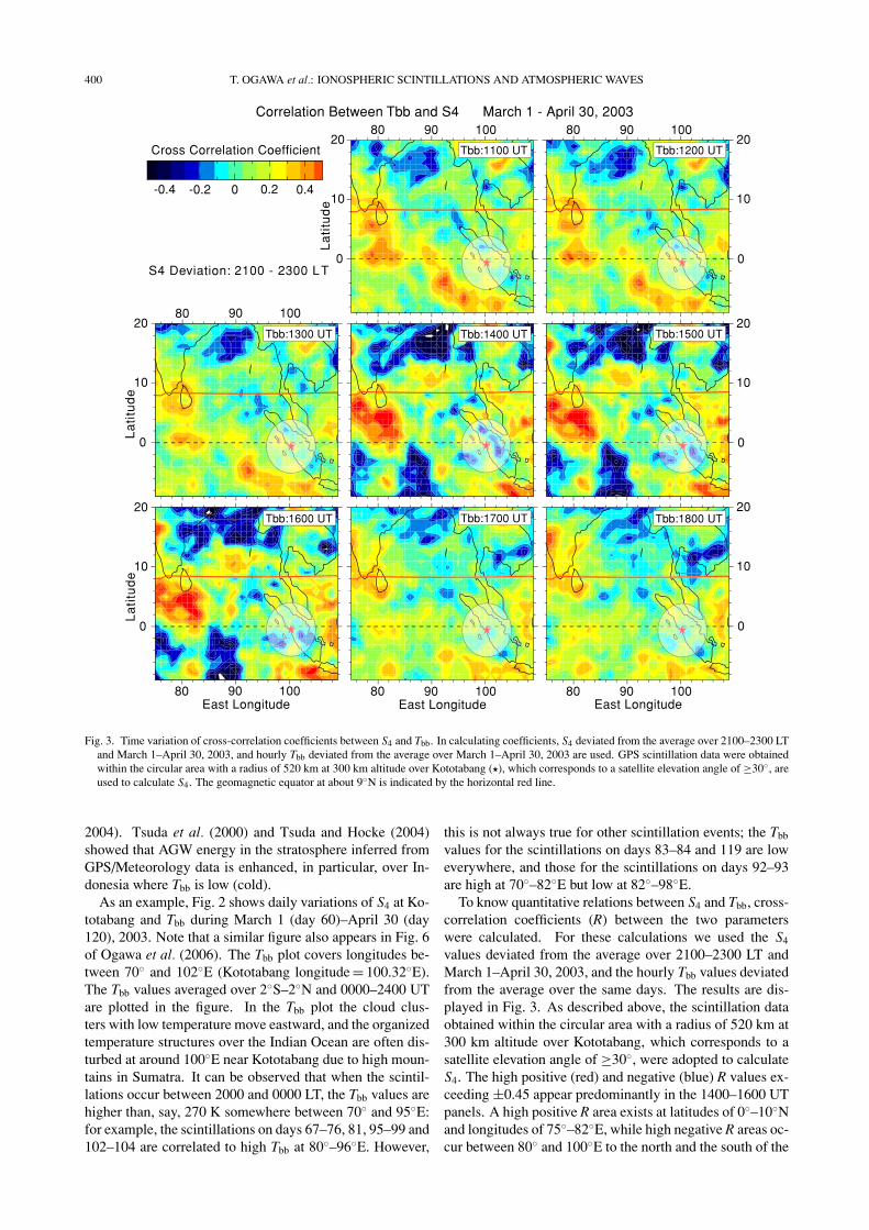
correspond well to the u′2 peaks at 92 km altitude during thesame days, and the S4 peaks between 2- and 8-day periodduring days 90–120 are also seen in the u′2 peaks at alti-tudes of 86 and 92 km during the same days. Figure 6(b)compares the wavelet spectra of S4 with Tbb spectra at theequator (0◦N) at four longitudes (80◦, 85◦, 90◦ and 95◦E)to the west of Kototabang. Some spectral peaks appearingbetween the 3- and 16-day period in the Tbb spectra are alsodiscerned in the S4 spectra.Figure 7 shows periodgrams of S4, Tbb and u′2 for the

wavelet power spectra shown in Fig. 6. The smooth thinsolid curves represent the 95% confidence level of thepower spectral density (PSD). The S4 and u′2 periodgramsin Fig. 7(a) exhibit spectral peaks at periods of about 2.5,5, 8, 14 and 25 days, and of about 2.5, 5, 7, 12–16 and22–25 days, respectively. The Tbb periodgrams in Fig. 7(b)have peaks at periods of about 5, 7 and 14 days. It is foundfrom Fig. 7 that some predominant periods seen in S4 havecounterparts in u′2 and Tbb, and that some predominant pe-riods appearing in Tbb do not always have counterparts inu′2 and S4. Similar wave periods are also discerned more orless in the seasons shown in Figs. 5(b), 5(c) and 5(d) (notshown). Thus, Figs. 6 and 7 suggest that the waves withperiods longer than 5 days, may be generated in the tro-posphere, can propagate upward to the lower thermosphere(92 km altitude) and may reach the ionosphere where theGPS scintillations originate. Note that the normal modeRossby waves have periods of 2, 5, 10 and 16 days (e.g.,Forbes, 1996). Since several spectral peaks of the S4 andu′2 fluctuations have periods similar to these waves, they

may be attributed to the upward propagation of PWs.

3. Simulation of Equatorial Atmospheric WavesIn Section 2, we have analyzed the data of S4 (GPS scin-

tillation index), u′2 (variance of zonal wind) at altitudes of86 and 92 km and Tbb (Earth’s black body temperature)to find that these parameters fluctuate with planetary-scalewave periods. However, it is very difficult to verify the exis-tence of such waves at ionospheric altitudes from our obser-vational data. To determine the behavior of neutral winds interms of PWs and AGWs that modulate them, we conductednumerical simulations using the Kyushu University GeneralCirculation Model (KUGCM): see Miyoshi and Fujiwara(2006, 2008) and Miyoshi (2006) for details. In brief, theKUGCM is a global spectral model with a triangular trun-cation of T85 (T21), which is equivalent to a grid spacing of1.4◦ (5.6◦) in latitude and longitude for a high (low) resolu-tion model. The low-resolution model was used only to ex-amine PWs with global scales. The region from the groundsurface to about 500 km altitude is divided into 75 verticallevels with a resolution of 0.4 × (atmospheric scale height)above the tropopause; i.e., the resolution is about 2, 8, 12and 17 km at 100, 150, 200 and 300 km altitude, respec-tively. The KUGCM includes a full set of the physical pro-cesses appropriate for the troposphere, stratosphere, meso-sphere and thermosphere, as well as schemes for hydrol-ogy, a boundary layer, radiation, eddy diffusion and moistconvection. It also includes cumulus and gravity wave pa-rameterizations, effects of the surface topography, amongothers. In the thermosphere the neutral composition is ob-

404 T. OGAWA et al.: IONOSPHERIC SCINTILLATIONS AND ATMOSPHERIC WAVES

12 30 366 24 42180

3

6

9

Frequency (cycles/day)

90 km100 km150 km200 km

2 0.64 1 Period (hours)1.5

oZonal Wind (0.4 N, 100 E) 10 Days in Late Marcho

0

3

6

9

0 0.2 0.4 0.6 1.00.8Frequency (cycles/day)

2 1.25510 Period (days)2.5

8

Periods: 0.5-12 hours

Periods: 1-100 days

PS

D (

m /

s )

22

90 km100 km150 km200 km

(b)

(a)

PS

D (

m /

s )

22

20

48

Fig. 8. Frequency spectra of zonal wind with periods of (a) 1–100 days and (b) 0.5–12 h at four altitudes simulated by high resolution KUGCM. 1- and0.5-day winds are not shown because of their strong power. Simulation data at (0.4◦N, 100◦E) for 10 days in late March are used.

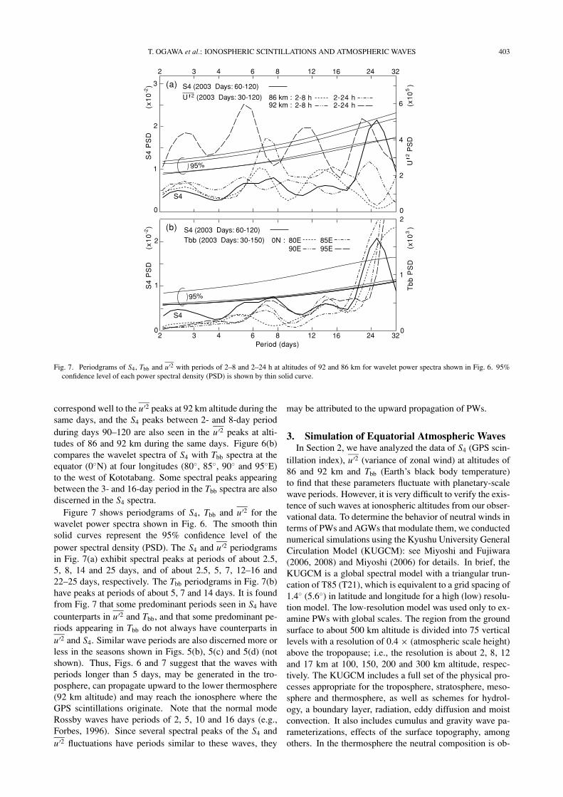
tained by solving the continuity equation for major species(N2, O2 and O), and infrared cooling, absorption of solarEUV and UV, ion drag, Joule heating and molecular dif-fusion are taken into account. A global electron densitydistribution model is also used. To exclude the effects ofday-to-day variations of solar EUV and UV fluxes and ge-omagnetic activity, the simulations were conducted undersolar cycle minimum and geomagnetically quiet conditions.In this paper, we discuss only zonal winds and waves be-cause these seem to be important for the seeding of plasmabubbles (e.g., Farley et al., 1986).3.1 Frequency spectrum of atmospheric wavesFigure 8 displays frequency spectra of the zonal wind

with periods of 1–100 days (Fig. 8(a)) and 0.5–12 h(Fig. 8(b)) at four altitudes from 90 to 200 km, whichare calculated from the high resolution (1.4◦) KUGCMdata at (0.4◦N, 100◦E) for 10 days in late March. InFig. 8(a), the waves with periods longer than ∼1 day dis-sipate quickly above 100 km and cannot propagate upwardbeyond 150 km. Contrary to this, the PSD of the 0.5- to3-hour waves in Fig. 8(b) increase with increasing altitude.The simulations indicate that these short-period waves canpropagate up to 400 km (see Figs. 11 and 12).To determine the detailed characteristics of the winds

shown in Fig. 8(a), Fig. 9 displays power spectra of the east-ward and westward propagating waves with periods longerthan 2 days at three altitudes in frequency-wave num-ber coordinates, which have been obtained from the low-resolution (5.6◦) KUGCM data at (2.8◦N, 0◦–360◦E) for1 year. Note that the spectral peaks at around zero frequencyare due to seasonal/1-year variations of the waves. Thewaves with periods of 2–20 days dissipate above 125 kmaltitude, as stated above (Fig. 8(a)). Several spectral peaks

can be observed below 125 km: the predominant ones areeastward propagating Kelvin waves with a 2-day periodwith zonal wave numbers K = +1 –+3 and westward prop-agating PWs with 6-day period with K = −1. The otherwaves are PWs with a 4-day period with K = −2, with 5-,10- and 16-day periods with K = −1 and with 2- to 2.5-dayperiods with K = −3 to −4. Note that the S4 periodgramin Fig. 7 indicates the spectral peaks at periods of about 2.5,5, 8, 14 and 25 days, which are partly consistent with thesimulation results.3.2 Time and altitude variations of atmospheric wavesIn this subsection we examine time and altitude vari-

ations of the equatorial wind simulated by the high-resolution (1.4◦) KUGCM. Figure 10 shows time variationsof zonal winds at (0.4◦N, 80◦E), (0.4◦N, 90◦E) and (0.4◦N,100◦E) at five altitudes from 150 to 350 km during 48 hin March 23–24. The winds fluctuate with time due to thewaves with periods of about 1–24 h. It is seen that the zonalwinds above 200 km altitude are, as a whole, eastward afterlocal sunset (∼1900 LT) until sunrise (∼0600 LT), with amaximum of about 80−1 near midnight, and westward in thedaytime with a maximum of about 80−1 near noon. Suchbehavior is mainly caused by a diurnal tide excited in thethermosphere.As shown in Fig. 8(b), the winds with periods of 0.5–

12 h become more evident with increasing altitude. In or-der to see the behavior of the short-period AGWs between1040 UT (1740 LT at Kototabang) and 1600 UT (2300 LT),Fig. 11 displays time variation in the zonal wind with pe-riods of 1–4 h at 0.4◦N during 1040–1600 UT (1740–2300 LT) on March 21 in longitude-altitude coordinates,which are simulated by the high resolution KUGCM. Thesolid (dotted) line contours indicate on eastward (westward)

T. OGAWA et al.: IONOSPHERIC SCINTILLATIONS AND ATMOSPHERIC WAVES 405

Frequency (cycles/day)

Wa

ven

um

be

r

Interval=1m/s2.5 days 5

1510 2.55

15

10

oZonal Wave (2.8 N, 0 -360 E) One Yearo o

Interval=0.4m/s

Interval=0.4m/s

Westward Eastward-0.1 0-0.3 -0.2 0.30.1 0.2 0.50.4-0.4-0.5

6

5

4

3

2

1

0

-0.1 0-0.3 -0.2 0.30.1 0.2 0.50.4-0.4-0.5

6

5

4

3

2

1

0

-0.1 0-0.3 -0.2 0.30.1 0.2 0.50.4-0.4-0.5

6

5

4

3

2

1

0

Wa

ven

um

be

rW

ave

nu

mb

er

h=100km

h=125km

h=150km

Fig. 9. Power spectra of eastward and westward propagating waves (periods ≥2 days) at three altitudes in frequency-wave number coordinatessimulated by low-resolution KUGCM. Simulation data at (2.8◦N, 0◦–360◦E) for 1 year are used. Spectral peaks at around zero frequency are due toseasonal/1-year variations of waves.

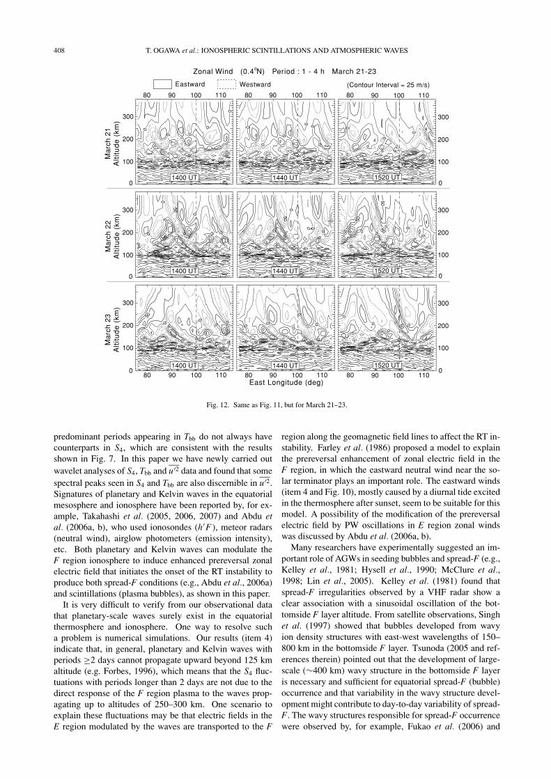
wind. Note that in the simulations the longitudinal resolu-tion is about 150 km and the altitudinal one changes from2 km at 100 km altitude to 17 km at 300 km altitude (seeabove). At altitudes of around 120–300 km, both eastwardand westward wind areas have scale lengths of about 300–1000 km (about 3◦–10◦ width) in longitude and about 30–100 km in altitude. They move, as a whole, eastward atabout 100−1 while changing the area patterns with time, inline with the results shown in Fig. 10. The velocities withinthe areas also change with time, with maximum eastwardand westward wind velocities of about 100−1. The windstructures seen in Fig. 11 change day by day. Figure 12shows time variations of the zonal winds with periods of 1–4 h between 1400 UT and 1520 UT on March 21–23. Thestructures and their eastward movement seen on March 21(Fig. 11) are also discerned on March 22 and 23. The struc-tures are more ordered on March 22 and 23 than March 21,and the wind velocities above 150 km altitude are fasteston March 22. Thus, Figs. 11 and 12 demonstrate that theactivity of the short-period AGWs in the equatorial thermo-sphere above 120 km altitude are changeable with time andday. It is noted that the wavy structures in the thermosphereabove 120 km altitude in Figs. 11 and 12 stem mainly fromthe ion drag and molecular viscosity, which also affect theupward propagation of PWs.

4. Summary and DiscussionThe results can be summarized as follows:

(1) 4.5-year observations of equatorial GPS scintillationsassociated with plasma bubbles indicate that scintil-lation activity clearly decreases with decreasing so-lar activity from 2003 to 2007. Scintillations appearpredominantly in equinoctial months, i.e. in March–April and September–October, and between 2000and 0100 LT in March–April and between 2000 and2300 LT in September–October. Scintillation occur-rences show clear day-to-day variability and appearmore often in March–April than September–October.

(2) Day-to-day comparison between S4 and Tbb shows thatthe scintillation occurrence can be related to Tbb varia-tion over the Indian Ocean to the west of Kototabang.Calculations of two-dimensional cross-correlation co-efficients (R) between S4 and Tbb indicate high posi-tive and negative R values exceeding ±0.45 appearingmainly at 1400–1600 UT (2100–2300 LT at Kotota-bang) at some localized areas (see Fig. 3). This resultsuggests that the scintillation occurrences before mid-night can be related, more or less, to the troposphericdisturbances over the Indian Ocean.

406 T. OGAWA et al.: IONOSPHERIC SCINTILLATIONS AND ATMOSPHERIC WAVES

oZonal Wind (0.4 N) March 23-24

h=200 km

h=250 km

h=300 km

h=350 km

0 6 12200

100

0

-100

200

100

0

-100

200

100

0

-100

200

100

0

-100

0 6 12

200

100

0

-100

Universal Time (hours)

Ea

stw

ard

Win

d (

m/s

)

7 13 19 1Local Time at 100 Eo

6 12

6 12

0 0

00

7 13 19 1 7

18 18

18 18

80 E90 E100 E

o

o

o

h=150 km

Fig. 10. Time variations of zonal winds at (0.4◦N, 80◦E), (0.4◦N, 90◦E) and (0.4◦N, 100◦E) at five altitudes during March 23–24 simulated byhigh-resolution KUGCM.

(3) Wavelet analyses of S4, u′2 and Tbb to determine thereasons of the day-to-day variability of the scintillationactivity indicate the following (1) S4 wavelet spectraexhibit some spectral peaks between the 2- and 15-day period and a peak at around the 24-day period.(2) Similar periods are also discerned in u′2 spectra.Some spectral peaks appearing between the 3- and 16-day period in Tbb are also recognized in S4. (3) In de-tail, wavelet periodgrams of S4 and u′2 exhibit spectralpeaks at periods of about 2.5, 5, 8, 14 and 25 days,and of about 2.5, 5, 7, 12–16 and 22–25 days, respec-tively. Tbb periodgrams have peaks at periods of about5, 7, and 14 days. These results suggest that long-period (≥2 days) atmospheric waves, i.e. planetary-scale waves, are responsible for the u′2 and S4 fluc-tuations.

(4) To determine the behavior of neutral winds in termsof PWs and short-period AGWs in the equatorial ther-mosphere, we conducted numerical simulations usingKUGCM. The results indicate the following (1) 2- to20-day waves dissipate rapidly above about 125 km,being unable to propagate upward further, and 0.5-

to 3-h waves become predominant with increasing al-titude beyond 100 km. (2) Below 125 km, west-ward propagating PWs exist with a period of 4 days(zonal wave number K = −2) and 5–6, 10 and 16 days(K = −1) in addition to 2- to 2.5-day waves (K = −3to −4), and eastward propagating Kelvin waves existwith periods of 2–5 days (K = +1 –+2). Figure 7 in-dicates the S4 spectral peaks at periods of about 2.5, 5,8, 14 and 25 days, which are partly consistent with thesimulation results. (3) Zonal winds above 200 km alti-tude at 80◦–100◦E near the equator are, on the whole,eastward after local sunset until sunrise, with a max-imum of about 80−1 near midnight, and westward inthe daytime with a maximum of about 80−1 near noon.Such a behavior is mainly due to a diurnal tide ex-cited in the thermosphere. (4) Zonal wind patterns, inaltitude-longitude coordinates, due to AGWs with pe-riods of 1–4 h above 120 km altitude, exhibit wavystructures with horizontal and vertical scale lengthsof about 300–1000 km and 30–100 km, respectively.They move, as a whole, eastward at about 100−1 whilechanging the structures with time. Wind direction

T. OGAWA et al.: IONOSPHERIC SCINTILLATIONS AND ATMOSPHERIC WAVES 407

(Contour Interval = 25 m/s)

Zonal Wind (0.4 N) Period : 1 - 4 h March 21o

Eastward Westward

Alt

itu

de

(km

)

East Longitude (deg)

300

200

100

0

300

200

100

0

50

90 100 110

50

50

90 100 110

50

300

200

100

090 100 110 90 100 110

-50

90 100 110

80 80

80 80 80

1040 UT 1120 UT 1200 UT

1240 UT 1320 UT 1400 UT

1440 UT 1520 UT 1600 UT

300

200

100

0

300

200

100

0

300

200

100

0

90 100 11080

0

0 0

0

000

0

0

0

0

0

0

0

0

00

0

00

0 00

0 0

0

0

0

0

00 0

0 0

Fig. 11. Time variation of zonal wind with periods of 1–4 h at 0.4◦N on March 21 in east longitude-altitude coordinates simulated by high-resolutionKUGCM. Solid (dotted) line contours indicate eastward (westward) wind. The longitude of Kototabang is shown by dashed line.

changes within such scale lengths. The wavy struc-tures change day by day.

The seasonal and yearly scintillation occurrence char-acteristics (item 1) are generally consistent with previousequatorial scintillation (bubble) observations (e.g., Basuand Basu, 1985; Basu et al., 1988; Burke et al., 2004; Gen-tile et al., 2006). The reason for the seasonal asymmetryis unknown. Eastward drifts of 350-m scale FAIs causingGPS scintillations also show the same seasonal asymmetry(Otsuka et al., 2006), i.e. the drifts between local sunsetand 2200 LT are faster in March–April than in September–October. Otsuka et al. (2006) speculate that this asym-metry is caused by seasonal asymmetry of neutral windsin the thermosphere. The seasonal occurrence pattern ofequatorial scintillations (bubbles) is known to depend onlongitude. In addition to the 350-m scale FAIs, bubblesare also accompanied by electron density irregularities withscale lengths of a few kilometers to tens of kilometers thatcause GPS total electron content (TEC) fluctuations (Beachand Kintner, 1999). Analyzing statistically the GPS data ofTEC fluctuations with such scale lengths obtained in India,Southeast Asia and Western Pacific, Ogawa et al. (2006)clarified that the scintillation occurrence patterns in 2003(Fig. 1) were quite similar to the bubble occurrence patternsover the Philippines, Singapore and Indonesia, but that they

deviate from those over Guam and India. More data ac-quisition for a full solar cycle is necessary to clarify thedetailed seasonal pattern at Kototabang, which is located inthe transition region between the Atlantic/Indian Ocean andPacific Ocean sectors. The solar cycle dependence of thescintillation occurrences can be explained by the changesin transequatorial thermospheric wind, background electricfield, vertical electron density gradient, electrical conduc-tivities in the E and F region, among others that controlthe excitation of the RT instability (e.g., Maruyama andMatuura, 1984; Sultan, 1996).As to item 2, Ogawa et al. (2006) also calculated cross

correlation coefficients between S4 and Tbb at 0◦N at fivelongitudes between 80◦–100◦E. They found that the coef-ficients during March 1–30 April 30, 2003, correspondingto Fig. 3 in this paper, decrease from +0.29 –+0.41 at 80◦

and 85◦E to +0.01 –+0.17 at 95◦E, which indicates thatthe scintillation occurrences over Kototabang may possiblybe affected by the tropospheric convective activity at longi-tudes of 80◦–90◦E. Figure 3 confirms in part these resultsand moreover suggests that the tropospheric convective ac-tivity at northern and southern latitudes some distance fromthe equator also affects the scintillation occurrences.As to item 3, using a FFT analysis, Ogawa et al. (2006)

found that S4 and Tbb have some common spectral peaksat periods between a few days and 13 days but that some

408 T. OGAWA et al.: IONOSPHERIC SCINTILLATIONS AND ATMOSPHERIC WAVES

-50

Ma

rch

22

Alt

itu

de

(km

)

East Longitude (deg)

300

200

100

0

90 100 110

300

200

100

0

90 100 110 90 100 110

300

200

100

0

300

200

100

090 100 110 90 100 11090 100 110

80 80 80

80 80 80

300

200

100

300

200

100

0

1400 UT 1440 UT 1520 UT

1400 UT 1440 UT 1520 UT

1400 UT 1440 UT 1520 UT

(Contour Interval = 25 m/s)

Zonal Wind (0.4 N) Period : 1 - 4 h March 21-23o

Eastward Westward

0

0

50

-50

50

-50

50

-50

5050

0

0

0

0

00

0

0

0

0

0

0

0

0

0

0

0

0 0

0

0

00

0

0

00

0

0 0

0

0

00 0 0

0

0

0

Ma

rch

23

Alt

itu

de

(km

)M

arc

h 2

1A

ltit

ud

e (

km)

Fig. 12. Same as Fig. 11, but for March 21–23.

predominant periods appearing in Tbb do not always havecounterparts in S4, which are consistent with the resultsshown in Fig. 7. In this paper we have newly carried outwavelet analyses of S4, Tbb and u′2 data and found that somespectral peaks seen in S4 and Tbb are also discernible in u′2.Signatures of planetary and Kelvin waves in the equatorialmesosphere and ionosphere have been reported by, for ex-ample, Takahashi et al. (2005, 2006, 2007) and Abdu etal. (2006a, b), who used ionosondes (h′F), meteor radars(neutral wind), airglow photometers (emission intensity),etc. Both planetary and Kelvin waves can modulate theF region ionosphere to induce enhanced prereversal zonalelectric field that initiates the onset of the RT instability toproduce both spread-F conditions (e.g., Abdu et al., 2006a)and scintillations (plasma bubbles), as shown in this paper.It is very difficult to verify from our observational data

that planetary-scale waves surely exist in the equatorialthermosphere and ionosphere. One way to resolve sucha problem is numerical simulations. Our results (item 4)indicate that, in general, planetary and Kelvin waves withperiods ≥2 days cannot propagate upward beyond 125 kmaltitude (e.g. Forbes, 1996), which means that the S4 fluc-tuations with periods longer than 2 days are not due to thedirect response of the F region plasma to the waves prop-agating up to altitudes of 250–300 km. One scenario toexplain these fluctuations may be that electric fields in theE region modulated by the waves are transported to the F

region along the geomagnetic field lines to affect the RT in-stability. Farley et al. (1986) proposed a model to explainthe prereversal enhancement of zonal electric field in theF region, in which the eastward neutral wind near the so-lar terminator plays an important role. The eastward winds(item 4 and Fig. 10), mostly caused by a diurnal tide excitedin the thermosphere after sunset, seem to be suitable for thismodel. A possibility of the modification of the prereversalelectric field by PW oscillations in E region zonal windswas discussed by Abdu et al. (2006a, b).Many researchers have experimentally suggested an im-

portant role of AGWs in seeding bubbles and spread-F (e.g.,Kelley et al., 1981; Hysell et al., 1990; McClure et al.,1998; Lin et al., 2005). Kelley et al. (1981) found thatspread-F irregularities observed by a VHF radar show aclear association with a sinusoidal oscillation of the bot-tomside F layer altitude. From satellite observations, Singhet al. (1997) showed that bubbles developed from wavyion density structures with east-west wavelengths of 150–800 km in the bottomside F layer. Tsunoda (2005 and ref-erences therein) pointed out that the development of large-scale (∼400 km) wavy structure in the bottomside F layeris necessary and sufficient for equatorial spread-F (bubble)occurrence and that variability in the wavy structure devel-opment might contribute to day-to-day variability of spread-F. The wavy structures responsible for spread-F occurrencewere observed by, for example, Fukao et al. (2006) and

T. OGAWA et al.: IONOSPHERIC SCINTILLATIONS AND ATMOSPHERIC WAVES 409

Saito and Maruyama (2007). Ogawa et al. (2005) foundthat bubbles with longitudinal spacings of 200–250 kmwere embedded within wavy plasma structures with scalesof a few hundreds to 1000 km. Rottger (1977, 1981)suggested that medium-scale traveling ionospheric distur-bances (MSTIDs), due to AGWs perhaps generated by con-vective activity in the intertropical convergence zone, had areasonable influence on the large-scale structure of spread-F irregularities and, hence, on plasma bubbles (see alsoMcClure et al., 1998). MSTID-like fluctuations that prop-agated southward were detected with an all-sky imager atKototabang by Shiokawa et al. (2006). From model cal-culations, Vadas and Fritts (2004) suggested that AGWswith sufficiently large vertical wavelengths and group ve-locities excited by mesoscale convective complexes at equa-torial latitudes can penetrate into the thermosphere, possi-bly contributing to the seeding of equatorial spread-F (seealso Vadas and Fritts, 2006; Vadas, 2007). Using the sameKUGCM as we have used in this paper, Miyoshi and Fuji-wara (2008) demonstrated that short-period (1.5–6 h) grav-ity waves with larger horizontal phase velocity (larger ver-tical wavelength) can penetrate into the thermosphere fromthe lower atmosphere and that day-to-day variability of hor-izontal wind fluctuations due to these gravity waves mayinduce ionospheric variability. Our simulations indicatethat AGWs with periods of 1–4 h can propagate into theequatorial ionosphere, being able to produce directly east-ward moving plasma structures with spatial scales of a fewtens to 1000 km, within which wind direction changes.Such plasma structures may be indirectly created througha process such that E region electric fields perturbed byAGWs are transported to the F region (e.g. Prakash, 1999).As shown in Fig. 12, the large-scale (a few hundreds to1000 km) horizontal wavy structures vary day by day, whichmay suggest that such a change in structure is responsiblefor the day-to-day variability of the GPS scintillation activ-ity.Apart from the AGW issue, Kudeki and Bhattacharyya

(1999) found a vortex plasma flow pattern at about 250 kmaltitude that was related to post-sunset bottomside spread-F events. A collisional shear instability, which is drivenby a plasma velocity shear, proposed by Hysell and Kudeki(2004) can produce large-scale (typically ∼200 km) wavestructures in the bottomside equatorial ionosphere (Hysellet al., 2004, 2006). We speculate that the vortical plasmaflow and velocity shear may originate from the wavy struc-tures shown in Figs. 11 and 12. To test this scenario, how-ever, it is necessary to calculate the electric field and plasmadrift caused by the neutral wind system that is simulated inthis paper.

5. ConclusionsWe have presented 4.5-year GPS ionospheric scintillation

observations at Kototabang, Indonesia with the aim of in-vestigating possible dynamical couplings between the iono-sphere/thermosphere and troposphere over the equator. Thescintillation activity is predominantly high between 2000and 0100 LT in equinoctial months with a seasonal asym-metry, and decreases with decreasing solar activity from

2003 to 2007, which is in line with previous equatorialscintillation (bubble) observations at other longitudes. TheS4 activity over Kototabang appears to be related to tropo-spheric disturbances over the Indian Ocean to the west ofKototabang. The scintillation index S4 shows clear day-to-day variability, with periods of about 2.5, 5, 8, 14 and25 days. Similar periods are also found in Earth’s bright-ness temperature Tbb and lower thermospheric neutral windu′2 variations, suggesting that S4 and u′2 are modulated bywaves with periods similar to PWs from below.The neutral wind system in the thermosphere simu-

lated by using KUGCM indicates the following: (1) 2-to 20-day waves, including planetary and Kelvin waves,dissipate rapidly above about 125 km, and 0.5- to 3-hwaves become predominant with increasing altitude beyond100 km, (2) zonal winds above 200 km altitude are, on thewhole, eastward after local sunset (∼1900 LT) until sunrise(∼0600 LT), (3) zonal wind patterns due to AGWs with pe-riods of 1–4 h above 120 km altitude exhibit wavy structureswith scale lengths of about 30–1000 km and, as a whole,move eastward at about 100−1 while changing the structureswith time. The wind direction changes within such scalelengths. The wavy structures change day by day. Thesesimulation results suggest that short-period gravity waves,which may contribute to the seeding of the RT instabilitygenerating plasma bubbles accompanied by scintillations,are generally present above 120 km altitude and that thebackground conditions necessary for the RT instability aremodulated by planetary-scale atmospheric waves. We sup-pose that such a scenario can explain the day-to-day vari-ability in the scintillation occurrences. Future work shouldinvestigate how ionospheric electric fields, electron densitydistribution, etc. are modulated with time, day and seasonby the simulated neutral winds.

Acknowledgments. GPS observations at the EAR site have beenconducted in collaboration with RISH of Kyoto University andLAPAN of Indonesia since September 2002. We are deeply grate-ful to the staff of LAPAN for their extensive collaborations to theobservations. We thank S. Sridharan and T. Yokoyama for theirhelp in the data analysis. Tbb data were supplied through KochiUniversity, Japan. This work is supported by Grant-in-Aid for Sci-entific Research on Priority Area-764 (13136201) of the Ministryof Education, Culture, Sports, Science and Technology of Japan,and partly by the 21st Century COE Program “Dynamics of theSun-Earth-Life Interactive System (SELIS)” of Nagoya Univer-sity.

ReferencesAbdu, M. A., Outstanding problems in the equatorial ionosphere-

thermosphere electrodynamics relevant to spread F , J. Atmos. Sol.-Terr.Phys., 63, 869–884, 2001.

Abdu, M. A., P. P. Batista, I. S. Batista, C. G. M. Brum, A. J. Carrasco,and B. W. Reinisch, Planetary wave oscillations in mesospheric winds,equatorial evening prereversal electric field and spread F , Geophys. Res.Lett., 33, L07107, doi:10.1029/2005GL024837, 2006a.

Abdu, M. A., T. K. Ramkumar, I. S. Batista, C. G. M. Brum, H. Takahashi,B. W. Reinisch, and J. H. Sobral, Planetary wave signatures in theequatorial atmosphere-ionosphere system, and mesosphere-E- an F-region coupling, J. Atmos. Sol.-Terr. Phys., 68, 509–522, 2006b.

Basu, Su. and S. Basu, Equatorial scintillations: Advances since ISEA-6,J. Atmos. Terr. Phys., 47, 753–768, 1985.

Basu, Su., S. Basu, J. P. MuClure, W. B. Hanson, and H. E. Whitney,High resolution topside in situ data of electron densities and VHF/GHzscintillations in the equatorial region, J. Geophys. Res., 88, 403–415,

410 T. OGAWA et al.: IONOSPHERIC SCINTILLATIONS AND ATMOSPHERIC WAVES

1983.Basu, S., E. MacKenzie, and Su. Basu, Ionospheric constraints of

VHF/UHF communications links during solar maximum and minimumperiods, Radio Sci., 23, 363–378, 1988.

Beach, T. L. and P. M. Kintner, Simultaneous Global Positioning Systemobservations of equatorial scintillations and total electron content fluc-tuations, J. Geophys. Res., 104, 22,553–22,565, 1999.

Burke, W. J., C. Y. Huang, L. C. Gentile, and L. Bauer, Seasonal-longitudinal variability of equatorial plasma bubbles, Ann. Geophys.,22, 3089–3098, 2004.

Farley, D. T., E. Bonelli, B. G. Fejer, and M. F. Larsen, The prereversalof the zonal electric field in the equatorial ionosphere, J. Geophys. Res.,91, 13,723–13,728, 1986.

Forbes, J. M., Planetary waves in the thermosphere-ionosphere system, J.Geomag. Geoelectr., 48, 91–98, 1996.

Fukao, S., Y. Ozawa, T. Yokoyama, M. Yamamoto, and R. T. Tsunoda,First observations of the spatial structure of F region 3-m-scale field-aligned irregularities with Equatorial Atmosphere Radar in Indonesia,J. Geophys. Res., 109, A02304, doi:10.1029/2003JA010096, 2004.

Fukao, S., T. Yokoyama, T. Tayama, M. Yamamoto, T. Maruyama, and S.Saito, Eastward traverse of equatorial plasma plumes observed with theEquatorial Atmosphere Radar in Indonesia, Ann. Geophys., 24, 1411–1418, 2006.

Gentile, L. C., W. J. Burke, and F. J. Rich, A global climatology forequatorial plasma bubbles in the topside ionosphere, Ann. Geophys., 24,163–172, 2006.

Hocke, K. and T. Tsuda, Gravity waves and ionospheric irregularitiesover tropical convection zones observed by GPS/MET radio occultation,Geophys. Res. Lett., 28, 2815–2818, 2001.

Hysell, D. L. and E. Kudeki, Collisional shear instability in the equa-torial F region ionosphere, J. Geophys. Res., 109, A11301, doi:10.1029/2004JA010636, 2004.

Hysell, D. L., M. C. Kelley, W. E. Swartz, and R. F. Woodman, Seedingand layering of equatorial spread F by gravity waves, J. Geophys. Res.,95, 17,253–17,260, 1990.

Hysell, D. L., J. Chun, and J. L. Chau, Bottom-type scattering layers andequatorial spread F, Ann. Geophys., 22, 4061–4069, 2004.

Hysell, D. L., M. F. Larsen, C. M. Swenson, and T. F. Wheeler, Shearflow effects at the onset of equatorial spread F, J. Geophys. Res., 111,A11317, doi:10.1029/2006JA011963, 2006.

Kelley, M. C., M. F. Larsen, C. LaHoz, and J. P. McClure, Gravity waveinitiation of equatorial spread F : A case study, J. Geophys. Res., 86,9087–9100, 1981.

Kudeki, E. and S. Bhattacharyya, Postsunset vortex in equatorial F-regionplasma drifts and implications for bottomside spread-F, J. Geophys.Res., 104, 28,163–28,170, 1999.

Lastovicka, J., Forcing of the ionosphere by waves from below, J. Atmos.Sol.-Terr. Phys., 68, 479–497, 2006.

Lin, C. S., T. J. Immel, H. C. Yeh, S. B. Mende, and J. L. Burch, Si-multaneous observations of equatorial plasma depletion by IMAGEand ROCSAT-1 satellites, J. Geophys. Res., 110, A06304, doi:10.1029/2004JA010774, 2005.

Maruyama, T. and N. Matuura, Longitudinal variability of annual changesin activity of equatorial spread F and plasma bubbles, J. Geophys. Res.,89, 10,903–10,912, 1984.

McClure, J. P., S. Singh, D. K. Bamgboye, F. S. Johnson, and H. Kil, Oc-currence of equatorial F region irregularities: Evidence for troposphericseeding, J. Geophys. Res., 103, 29,119–29,135, 1998.

Miyoshi, Y., Temporal variation of nonmigrating diurnal tide and its rela-tion with the moist convective activity, Geophys. Res. Lett., 33, L11815,doi:10.1029/2006GL026702, 2006.

Miyoshi, Y. and H. Fujiwara, Excitation mechanism of intraseasonal oscil-lation in the equatorial mesosphere and lower thermosphere, J. Geophys.Res., 111, D14108, doi:10.1029/2005JD006993, 2006.

Miyoshi, Y. and H. Fujiwara, Gravity waves in the thermosphere simulatedby a general circulation model, J. Geophys. Res., 113, D01101, doi:10.1029/2007JD008874, 2008.

Ogawa, T., E. Sagawa, Y. Otsuka, K. Shiokawa, T. J. Immel, S. B. Mende,and P. Wilkinson, Simultaneous ground- and satellite-based airglowobservations of geomagnetic conjugate plasma bubbles in the equatorialanomaly, Earth Planets Space, 57, 385–392, 2005.

Ogawa, T., Y. Otsuka, K. Shiokawa, A. Saito, and M. Nishioka, Iono-spheric disturbances over Indonesia and their possible association withatmospheric gravity waves from the troposphere, J. Meteor. Soc. Jpn.,84A, 327–342, 2006.

Otsuka, Y., K. Shiokawa, T. Ogawa, and P. Wilkinson, Geomagnetic conju-gate observations of equatorial airglow depletions, Geophys. Res. Lett.,

29(15), doi:10.1029/2002GL015347, 2002.Otsuka, Y., K. Shiokawa, T. Ogawa, T. Yokoyama, M. Yamamoto, and

S. Fukao, Spatial relationship of equatorial plasma bubbles and field-aligned irregularities observed with an all-sky airglow imager andthe Equatorial Atmosphere Radar, Geophys. Res. Lett., 31, L20802,doi:10.1029/2004GL020869, 2004.

Otsuka, Y., K. Shiokawa, and T. Ogawa, Equatorial ionospheric scintil-lations and zonal irregularity drifts observed with closely-spaced GPSreceivers in Indonesia, J. Meteor. Soc. Jpn., 84A, 343–351, 2006.

Prakash, S., Production of electric field perturbations by gravity wavewinds in the E region suitable for initiating equatorial spread F, J.Geophys. Res., 104, 10,051–10,069, 1999.

Rottger, J., Travelling disturbances in the equatorial ionosphere and theirassociation with penetrative cumulus convection, J. Atmos. Terr. Phys.,39, 987–998, 1977.

Rottger, J., Equatorial spread-F by electric fields and atmospheric gravitywaves generated by thunderstorms, J. Atmos. Terr. Phys., 43, 453–462,1981.

Saito, S. and T. Maruyama, Large-scale longitudinal variation inionospheric height and equatorial spread F occurrences observedby ionosondes, Geophys. Res. Lett., 34, L16109, doi:10.1029/2007GL030618, 2007.

Shiokawa, K., Y. Otsuka, T. Ogawa, and P. Wilkinson, Time evolution ofhigh-altitude plasma bubbles imaged at geomagnetic conjugate points,Ann. Geophys., 22, 3137–3143, 2004.

Shiokawa, K., Y. Otsuka, and T. Ogawa, Quasiperiodic southward movingwaves in 630-nm airglow images in the equatorial thermosphere, J.Geophys. Res., 111, A06301, doi:10.1029/2005JA011406, 2006.

Singh, S., F. S. Johnson, and R. A. Power, Gravity wave seeding of equa-torial plasma bubbles, J. Geophys. Res., 102, 7399–7410, 1997.

Sridharan, S., T. Tsuda, R. A. Vincent, T. Nakamura, and Effendy, A reporton radar observations of 5–8-day waves in the equatorial MLT region,J. Meteor. Soc. Jpn., 84A, 295–304, 2006.

Sultan, F. J., Linear theory and modeling of the Rayleigh-Taylor instabilityleading to the occurrence of equatorial spread F, J. Geophys. Res., 101,26,875–26,891, 1996.

Takahashi, H., L. M. Lima, C. W. Wrasse, M. A. Abdu, I. S. Batista, D.Gobbi, R. A. Buriti, and P. P. Batista, Evidence on 2–4 day oscillationsof the equatorial ionosphere h′ F and mesospheric airglow emissions,Geophys. Res. Lett., 32, L12102, doi:10.1029/2004GL022318, 2005.

Takahashi, H., C. W. Wrasse, D. Pancheva, M. A. Abdu, I. S. Batista, L.M. Lima, P. P. Batista, B. R. Clemesha, and K. Shiokawa, Signatures of3–6 day planetary waves in the equatorial mesosphere and ionosphere,Ann. Geophys., 24, 3343–3350, 2006.

Takahashi, H. et al., Signatures of ultra fast Kelvin waves in the equatorialmiddle atmosphere and ionosphere, Geophys. Res. Lett., 34, L11108,doi:10.1029/2007GL029612, 2007.

Tsuda, T. and K. Hocke, Application of GPS radio occultation data forstudies of atmospheric waves in the middle atmosphere and ionosphere,J. Meteor. Soc. Jpn., 82, 419–426, 2004.

Tsuda, T., M. Nishida, C. Rocken, and R. H.Ware, A global morphology ofgravity wave activity in the stratosphere revealed by the GPS occultationdata (GPS/MET), J. Geophys. Res., 105, 7257–7273, 2000.

Tsunoda, R. T., On the enigma of day-to-day variability in the equa-torial spread F, Geophys. Res. Lett., 32, L08103, doi:10.1029/2005GL022512, 2005.

Vadas, S. L., Horizontal and vertical propagation and dissipation of gravitywaves in the thermosphere from lower atmospheric and thermosphericsources, J. Geophys. Res., 112, A06305, doi:10.1029/2006JA011845,2007.

Vadas, S. L. and D. C. Fritts, Thermospheric responses to gravity wavesarising from mesoscale convective complexes, J. Atmos. Sol.-Terr.Phys., 66, 781–804, 2004.

Vadas, S. L. and D. C. Fritts, Influence of solar variability on gravity wavestructure and dissipation in the thermosphere from tropospheric convec-tion, J. Geophys. Res., 111, A10S12, doi:10.1029/2005JA011510, 2006.

Woodman, R. F. and C. LaHoz, Radar observations of F region equatorialirregularities, J. Geophys. Res., 81, 5447–5466, 1976.

Yokoyama, T., S. Fukao, and M. Yamamoto, Relationship of the onset ofequatorial F region irregularities with the sunset terminator observedwith the Equatorial Atmosphere Radar, Geophys. Res. Lett., 31, L24804,doi:10.1029/2004GL021529, 2004.

T. Ogawa (e-mail: taogawa@nict.go.jp), Y. Miyoshi, Y. Otsuka, T.Nakamura, and K. Shiokawa