Sonderforschungsbereich/Transregio 15 · www.gesy.uni-mannheim.de Universität Mannheim · Freie Universität Berlin · Humboldt-Universität zu Berlin · Ludwig-Maximilians-Universität München

Rheinische Friedrich-Wilhelms-Universität Bonn · Zentrum für Europäische Wirtschaftsforschung Mannheim

Speaker: Prof. Konrad Stahl, Ph.D. · Department of Economics · University of Mannheim · D-68131 Mannheim, Phone: +49(0621)1812786 · Fax: +49(0621)1812785

May 2006

*Kai A. Konrad, WZB, Reichpietschufer 50, D-10785 Berlin, Germany, e-mail: kkonrad@wz-berlin.de **Dan Kovenock, Krannert School of Management, Purdue University, West Lafayette, IN 47907, USA,

fax: +1-765-494-9658, e-mail: kovenock@purdue.edu

Financial support from the Deutsche Forschungsgemeinschaft through SFB/TR 15 is gratefully acknowledged.

Discussion Paper No. 121

Equilibrium and Efficiency in the Tug-of-War Kai A. Konrad*

Dan Kovenock**

Equilibrium and Efficiency in the Tug-of-War∗

Kai A. Konrad†and Dan Kovenock‡

May 16, 2006

AbstractWe characterize the unique Markov perfect equilibrium of a tug-of-

war without exogenous noise, in which players have the opportunity toengage in a sequence of battles in an attempt to win the war. Eachbattle is an all-pay auction in which the player expending the greaterresources wins. In equilibrium, contest effort concentrates on at mosttwo adjacent states of the game, the "tipping states", which are de-termined by the contestants’ relative strengths, their distances to finalvictory, and the discount factor. In these states battle outcomes arestochastic due to endogenous randomization. Both relative strengthand closeness to victory increase the probability of winning the battleat hand. Patience reduces the role of distance in determining outcomes.Applications range from politics, economics and sports, to biology,

where the equilibrium behavior finds empirical support: many specieshave developed mechanisms such as hierarchies or other organizationalstructures by which the allocation of prizes are governed by possiblyrepeated conflict. Our results contribute to an explanation why. Com-pared to a single stage conflict, such structures can reduce the overallresources that are dissipated among the group of players.Keywords: winner-take-all, all-pay auction, tipping, multi-stage con-

test, dynamic game, preemption, conflict, dominance.JEL classification numbers: D72, D74

∗Corresponding author: Kai A. Konrad, WZB, Reichpietschufer 50, D-10785 Berlin, Ger-many, e-mail: kkonrad@wz-berlin.de. Comments by Daniel Krähmer and Johannes Münsterare gratefully acknowledged. Part of this work was completed while the second author wasVisiting Professor at the Social Science Research Center Berlin (WZB). Konrad acknow-ledges funding from the German Science Foundation (DFG, grant no. SFB-TR-15). Theusual caveat applies.

†Free University of Berlin and Social Science Research Center Berlin (WZB).‡Krannert School of Management, Purdue University.

1

1 Introduction

Final success or failure in a conflict is often the result of the outcomes ofa series of potential battles. An illustrative example is the decision makingprocess in many organizations. Resources, jobs and other goods that involverents to individuals inside the organization are frequently allocated in a processthat has multiple decision stages. For instance, hiring decisions often involvea contest between candidates in which a hiring committee makes a decisionand forwards this decision to another committee. This committee approves tothe initial decision and forwards the case further until a final decision stage isreached, or may return the case to the previous committee. Two competingcandidates could expend effort trying to influence the decision process in eachstage. Such multi-layered decision processes obviously cause delay in decisionmaking and this can be seen as a cost. We will argue here that, compared to asingle stage decision process in which the rival players spend effort in a singlestage all-pay auction, the multi-stage decision process can be advantageous asit may improve allocative efficiency and reduce effort that is expended by rivalcontestants in the conflict.In more general terms we describe the multi-stage contest as a tug-of-war.

It consists of a (possibly infinite) sequence of battles between two contestantswho accumulate stage victories, and in which the contestant who first accu-mulates a sufficiently larger number of such victories than his rival is awardedthe prize for final victory. To our knowledge, Harris and Vickers (1987) werethe first to look formally at the tug-of-war. They analyse an R&D race as atug-of-war in which each single battle is determined as the outcome of a con-test with noise. The exogenous noise allows for deterministic equilibrium effortchoices in each battle, but, at the same time, makes the problem less tractableand has so far ruled out a fully analytic description of the equilibrium. Budd,Harris and Vickers (1993) apply a somewhat more complicated stochastic dif-ferential game approach to a dynamic duopoly, seen as a tug-of-war involvinga continuum of advertizing or R&D battles that determine the firms’ relativemarket positions. Using a complementary pair of asymptotic expansions forextreme parameter values and numerical simulations elsewhere, they isolatea number of effects that govern the process. Several of these appear in ouranalysis which, unlike their framework, derives an analytical solution for theunique Markov perfect equilibrium. Moreover, our analysis of battles withoutnoise leads to an equilibrium with mixed strategies and allows us to explicitlysolve for equilibrium for both symmetric and asymmetric environments.

2

We examine how the players’ respective fighting abilities, rewards from finalvictory, and the distances in terms of the required battle win differential toachieve victory interact to determine Markov perfect equilibrium behavior inthe tug-of-war. For notational convenience we concentrate on the asymmetryin the valuations of the final prize and assume equal fighting ability, but aswill be shown this is equivalent to the more general case with asymmetricvaluations of the prize and asymmetric fighting abilities. We show that thecontest effort that is dissipated in total and over all battle periods cruciallydepends on the starting point of the tug-of-war, and, for many starting points,is negligible, even if the asymmetry in the starting conditions is very limited.The multi-battle structure in a tug-of-war reduces the amount of resources

that is dissipated in the contest, compared to a single all-pay auction, whichhas been studied more carefully in the literature. Key references are Hillmanand Riley (1989) and Baye, Kovenock and deVries (1993, 1996) for the case ofcomplete information, and Amann and Leininger (1995, 1996), Krishna andMorgan (1997), Kura (1999), Moldovanu and Sela (2001) and Gavious, Mol-dovanu and Sela (2002) in the context of incomplete information.1 A repeatedall-pay auction has been considered by McAfee (2000). Apart from the use ofa different tie-breaking rule, a difference between our and his analysis is hisassumption that the final loser in the tug-of-war receives a strictly negativeprize, compared to a loser prize of zero in this paper. With negative loserprizes, the loser would like to delay final defeat, even if this delay does not im-ply or open up a chance for this player to turn defeat into victory. In contrast,with a loser prize of zero, when the tug-of-war ends, the loser sacrifices onlythe option to win the winner prize, but does not suffer more from terminationnow than from termination tomorrow. With negative loser prizes, contestantsmay continue the tug-of-war with negligible fighting effort forever, but the in-tensity of fighting picks up once the process moves close to final defeat of oneof the contestants. In contrast, with non-negative loser prizes, fighting takesplace only at stages where neither of the contestants has a major advantage.As a modeling device, the tug-of-war has a large number of applications in

diverse areas of science, including political science, economics, astronomy andhistory.2 The term ‘tug-of-war’ has also been used in biology. In the context

1For further applications of the all-pay auction see Arbatskaya (2003), Baik, Kim andNa (2001), Baye, Kovenock and De Vries (2005), Che and Gale (1998, 2003), Ellingsen(1991), Kaplan, Luski and Wettstein (2003), Konrad (2004), Moldovanu and Sela (2004),and Sahuguet and Persico (2005).

2To give a few examples: In politics, Whitford (2005) describes the struggle between the

3

of within-group conflict among animals, subjects could struggle repeatedly.3

For instance, the formation of hierarchies and their dynamic evolution oc-curs in repeated battle contests. As Hemelrijk (2000) describes for severalexamples, individuals may try to acquire a high rank, but the differentiationand asymmetry that is created by this can also reduce future conflict. Win-ning or losing a particular contest in a series of conflictual situations is knownto change future conflict behavior (Bergman et al. (2003), Beacham (2003)and Hsu and Wolf (1999)). This may partially be the result of informationabout own fighting skills and the fighting experience gained, but it may alsoarise from the change in strategic position with respect to future conflict aboutrank, territory, access to food, or opportunities to reproduce.Evidence from biology and political science shows that violent conflict often

does not take place, or, at least, the intensity of a conflict varies significantlyas a function of the conflicting parties’ actual strengths, previous experience,and the strategic symmetry or asymmetry of the particular situation in termsof territorial or other advantages. There are probably examples in line withthe result in McAfee, where fighting effort increases when the tug-of-war ap-proaches one of the end points. However, there are also situations in whichfighting occurs only in an interior state in which the players are sufficientlysymmetric. Parker and Rubenstein (1981) and Hammerstein (1981), for in-

president and legislature about the control of agencies as a tug-of-war. Yoo (2001) refers tothe relations between the US and North-Korea and Organski and Lust-Okar (1997) to thestruggle about the status of Jerusalem as cases of tug-of-war. According to Runciman (1987),at the time of the Crusades, when various local rulers frequently attacked one another, theysometimes succeeded in conquering a city or a fortification, only to lose this, or another,part of their territory to the same, or another, rival ruler later on. The conflict between tworival rulers can be seen as a sequence of battles. They start at some status quo in whicheach rules over a number of territories with fortified areas. They fight each other in battles,and each battle is concerned with one fortress or territory. In the sequence of successes andfailures, the fortresses or territories are destroyed or reallocated, and the conflict continuesuntil one of the rulers has lost all his fortresses or territories and is thus finally defeated.If battle success alternates more or less evenly, then such a contest can go on for a verylong time, possibly even forever. The end comes only when one of the rulers has been moresuccessful than his rival sufficiently often.

3The term also refers to contests between different species. Ehrenberg and McGrath(2004) refer to the interaction of microtubule motors, Larsson, Beignon and Bhardwaj (2004)and Zhou et al. (2004) refer to the interaction between viruses and the dendritic cells orother parts of the immune system as tugs of war. Tibbetts and Reeve (2000) consider therole of the amount of reproductive sharing within a group for the likelihood of within-groupconflict among the social wasp Polistes dominulus.

4

stance, emphasize the role of asymmetry in determining whether a conflictualsituation turns into a resource wasteful or violent conflict, with symmetrymaking fighting more likely. Different advantages and disadvantages may de-termine the overall asymmetry of a conflictual situation, and counterbalanceor add to each other. Schaub (1995) describes the conflict over food that oc-curs between long-tailed macaque females. Differences in strength and in thedistances between the animals and the location of the food govern their beha-vior. Superior strength or dominance of one contestant can be compensatedby a greater distance she has to the location of the food. Relative strength,together with the actual payoffs from winning determine contestants’ stakesat any given stage of a tug-of-war and determine the degree of asymmetrybetween the rival players.Our results may contribute to explaining why mechanisms such as hierarch-

ies or other organizational structures have evolved by which the allocation ofprizes is governed by a multi-stage conflict.4 Such structures may delay theallocation of a given prize, compared to a single stage conflict, but can con-siderably reduce the overall resources that are dissipated among the group ofplayers. Compared to a standard all-pay auction, a tug-of-war that is notrigged in favor of one of the players also improves allocative efficiency; theprobability with which the prize is awarded to the player who values it morehighly is higher in the tug-of-war than in the standard all-pay auction.In the next section we outline the structure of the tug-of-war and char-

acterize the unique Markov perfect equilibrium. In section 3 we discuss theefficiency properties of the tug-of-war and compare it with the all-pay auction.Section 4 concludes.

4There are, of course, other explanations for hierarchies more generally, which, however,focus on different aspects of a hierarchy (see, e.g., the survey in Radner 1992). Radner(1993) for instance, considers a problem of efficient information aggregation, asking what isthe efficient decision tree. Closer to the issue of allocation of goods in a conflict, Wärneryd(1998) and Müller and Wärneryd (2001) consider distributional conflict between rival groupsfollowed by distributional conflict within the winning group as a type of hierarchical conflict.Both these approaches focus on the "tree-" or "pyramid"-property of hierarchies that reducesthe number of players when moving to the top, whereas our approach does not use thisproperty. We consider only two contestants throughout and focus on the sequential, repeatednature of decision process.

5

2 The analytics of the tug-of-war

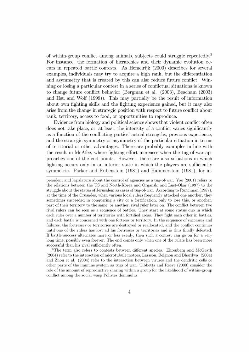
A tug-of-war is a multi-stage game with a potentially infinite horizon whichis characterized by the following elements. The set of players is {A,B}. Theset of states of the war is given by a finite ordered grid of m + 1 pointsM ≡ {0, 1, ...m} in R1. The tug-of-war begins at time t = 1 with playersin the intitial state j(1) = mA, 0 < mA < m, which may either be chosenby nature, or may be a feature of the institutional design. In each periodt = 1, 2, 3... a battle takes place between the players in which A (resp. B)expends effort at (resp. bt). A victory by player A (B) in state i at time tmoves the war to state i− 1 (i+ 1) at time t+ 1. The state in period t+ 1 istherefore j(t + 1) = mA + nBt − nAt, where nAt and nBt denote respectively,the number of battle victories that A and B have accumulated by the endof period t. This continues as long as the war stays in some interior statej ∈M int ≡ {1, 2, ..., (m− 1)}. The war ends when one of the players achievesfinal victory by driving the state to his favored terminal state, j = 0 andj = m, for player A and B respectively. A prize (for final victory) of sizeZA > 0 is awarded to A if the terminal state j = 0 is reached, and B receives aloser prize equal to zero at this state. Alternatively, a winner prize of ZB > 0is awarded to B if the terminal state j = m is reached, and A receives a loserprize of zero in this case. Without loss of generality we assume that ZA ≥ ZB.5

states j m m-1 mA-1 mA+1 mA 0 1

... ...

Figure 1:

Figure 1 depicts the set of states. PlayerA’s (B’s) period t payoff πA(at, j(t))(πB(bt, j(t))) is assumed to equal ZA (ZB) if player A (B) is awarded the prizein that period, and −at (−bt) if t is a period in which effort is expended.6 Weassume that each player maximizes the expected discounted sum of his per-

5Qualitatively similar results can be obtained for sufficiently small but positive loserprizes. The assumption that the loser prizes are non-negative is crucial for the results. Theanalysis with negative loser prizes is carried out in McAfee (2000).

6Since the per-period payoffs do not depend directly on time, we have dropped a timeindex.

6

period payoffs. Throughout we assume that 0 < δ < 1 denotes the common,time invariant, discount factor.7

The assumption that the cost of effort is simply measured by the effortitself is for notational simplicity only. Since a player’s preference over incomestreams is invariant with respect to a positive affine transformation of utility,if player A (B) has a constant unit cost of effort cA (cB) we may normalizeutility by dividing by cA (cB) to obtain a new utility function representing thesame preferences in which the unit cost of effort is 1 but player A (B) has aprize value ZA/cA (ZB/cB). Therefore, our model with asymmetric prizes canbe interpreted as one with both asymmetric prizes and fighting abilities.Each single battle in the tug-of-war is a simultaneous move all-pay auction

with complete information. A player’s action in each period in which the stateis interior is his effort, at ∈ [0, K] and bt ∈ [0, K], for A and B, respectively,where K ≥ ZA.8 The player who spends the higher effort in a period wins thebattle. We choose a deterministic tie-breaking rule for the case in which bothplayers choose the same effort, by which the ”advantaged” player wins. Givenm, ZA, ZB and δ, we say that player A is advantaged in state j if δjZA >δm−jZB, and B is advantaged if δjZA ≤ δm−jZB. We define j0 = min{j ∈M int

¯̄δjZA ≤ δm−jZB } where this is non-empty, and j0 = m otherwise: player

B is advantaged for j ∈M int such that j ≥ j0 and A is advantaged otherwise.If m = 2 and mA = 1, the tug-of-war reduces to the well-known case of

the standard all-pay auction with complete information at time t = 1, as inHillman and Riley (1989), Ellingsen (1991) or Baye, Kovenock and deVries(1996). In this case, one single battle takes place at state j = mA = 1. Theprocess moves from this state in period 1 to j = 0 or to j = 2 at the beginningof period 2, and the prize is handed over to A or B, respectively. Accordingly,the contest at period t = 1 in state j = 1 is over a prize that has a presentvalue of δZA and δZB for A and B, respectively, and the payoffs in the uniqueequilibrium of this game (which are in nondegenerate mixed strategies) areδ(ZA − ZB) for A and zero for B. In what follows, we consider the case withm > 2.For each period t, if a terminal state has not yet been reached by the

beginning of the period, players simultaneously choose efforts with common

7It is straightforward to extend our results to cases in which players have different, timeinvariant discount factors δA and δB.

8This upper limit makes the set of possible effort choices compact, but does not lead toa restriction that could be binding in any equilibrium, as an effort choice larger than ZA insome period is strictly dominated by a choice of effort of zero in this and all future periods.

7

knowledge of the initial state mA and the full history of effort choices, denotedas (at−1,bt−1) ≡ ((a1, ..., at−1), (b1, ..., bt−1)). Players also know the currentstate j(t) of the war and the state in any past period j(τ), τ < t. We definejt = (j(1), j(2), ...j(t)), where j(1) = mA. Hence, we will summarize thehistory at time t along any path which has not yet hit a terminal state byht = (at−1,bt−1, jt). We will call such a path a non-terminal period t historyand will denote the set of such histories by Ht. A history of the game thatgenerates a path that reaches a terminal state at precisely period t is termeda terminal period t history. Denote the set of terminal period t histories byT t, and the set of (at−1,bt−1) generating elements of T t by T t

e .If for an infinite sequence of effort choices, a = (a1, a2, ...) and b =

(b1, b2, ...) no terminal state is reached in finite time, we will call the cor-responding history h∞ = (a,b, j) a non-terminal history and denote the set ofsuch histories as H∞.Given these constructions, we define a behavior strategy σl for player l ∈

{A,B} as a sequence of mappings σl(ht) : Ht → Σ[0,K], that specifies forevery period t and non-terminal history ht an element of the set of probabilitydistributions over the feasible effort levels [0, K]. Each behavior strategy profileσ = (σA, σB) generates for each t a probability distribution over histories inthe set

Sτ≤t T

τ ∪Ht. It also generates a probability distribution over the setof all feasible paths of the game,

S∞τ=1 T

τ ∪H∞.Since we assume that each player’s payoff for the tug-of-war is the expec-

ted discounted sum of his per-period payoffs, the payoff for player A from abehavioral strategy profile σ is denoted vA(σ) = Eσ(Σ

t̃t=1δ

t−1πA(at, j(t))) ≡Eσ(πA(at̃−1,bt̃−1, jt̃)) where t̃ is the hitting time at which a terminal state isfirst reached.9 If a terminal state is never reached, t̃ = ∞. Note that fora given sequence of actions (at̃−1 bt̃−1), t̃ arises deterministically, accordingto the non-random transition rule embodied in the all-pay auction, so thatthe randomness of t̃ is generated entirely by the non-degenerate nature of theprobability distributions chosen by the behavioral strategies. If ht+1 = (atbt, jt+1) ∈ T t+1

e denotes a sequence of efforts that leads to a terminal state atprecisely period t̃ = t+ 1, then, the payoffs for A and B are

9We adopt a notational convention throughout this paper that the action set availableto each player in a terminal state is the effort level zero, so that for any hitting time t̃,at̃ = bt̃ = 0. Hence, in these states πA(at, j) and πB(bt, j) include only the prize awardedto the victor, and we suppress the terms at̃ and bt̃ in the notation Σ

t̃t=1δ

t−1πA(at, j(t)) ≡πA(at̃−1,bt̃−1, jt̃).

8

πA((at,bt, jt+1)) =

⎧⎪⎪⎪⎪⎨⎪⎪⎪⎪⎩−

tXi=1

δi−1ai +δtZA if j(t+ 1) = 0

−tX

i=1

δi−1ai if j(t+ 1) = m

(1)

and, respectively,

πB((at,bt, jt+1)) =

⎧⎪⎪⎪⎪⎨⎪⎪⎪⎪⎩−

tXi=1

δi−1ai +δtZB if j(t+ 1) = m

−tX̂i=1

δi−1ai if j(t+ 1) = 0.

(2)

If for an infinite sequence of effort choices, a = (a1, a2, ...) and b = (b1, b2, ...)no terminal state is reached in finite time, payoffs are

πA((a,b, j)) = −∞Xt=1

δt−1at and πB((a,b, j)) = −∞Xt=1

δt−1bt.

For a given behavior strategy profile σ = (σA, σB) each player’s payoff in thetug-of-war can be derived from calculating the expected sum of discountedper period payoffs generated by the probability distribution over histories inthe set

S∞τ=1 T

τ ∪ H∞. Moreover, for any t and ht ∈ Ht, one may defineeach player’s expected discounted value of future per-period payoffs (discoun-ted back to time t) conditional on the history ht by deriving the conditionaldistribution induced byσ|ht over

S∞τ=t+1 T

τ ∪ H∞. We shall refer to this asa player’s continuation value conditional on ht and denote it by vi(σ |ht ) =Eσ|ht(Σt̃

s=tδs−tπA(as, j(s))). Note that this has netted out any expenditures

accrued on the history ht.Since the players’ objective functions are additively separable in the per-

period (time invariant) payoffs and transitions probabilities depend only uponthe current state and actions, continuation payoffs from any sequence of cur-rent and future action profiles depend on past histories only through thecurrent state j. It therefore seems natural to restrict attention to Markovstrategies that depend only on the current state j and examine the set ofMarkov perfect equilibria. Indeed, this partition of histories is that obtained

9

from the more formal analysis of the determination of the Markov partitionin Maskin and Tirole (2001). For any t, we may partition past (non-terminal)histories in Ht by the period t state j(t), inducing a partition Ht(·), and definethe collection of partitions, H(·) ≡ {Ht(·)}∞t=1. It can be demonstrated that inour game the vector of collections (HA(·), HB(·)) = (H(·), H(·)) is the uniquemaximally coarse consistent collection (the Markov collection of partitions) inthe sense of Maskin and Tirole (2001, p. 201). For any time t, the current statej(t) therefore constitutes what they call the payoff-relevant history. Since ourgame is stationary, we may partition the set of all finite non-terminal historiesby the same state variables, j ∈M int ≡ {1, 2, ...(m−1)}, removing any depend-ence of the partition on the time t. We label this partition {j(t) = i}i∈Mint.This is the stationary partition defined by Maskin-Tirole, (2001, p. 203).In the continuation, we restrict attention to (stationary) Markov strategies

measurable with respect to the payoff relevant history determined by the sta-tionary partition {j(t) = i}i∈Mint. A stationary Markov strategy σl for playerl ∈ {A,B} is a mapping σl(j) :M int → Σ[0,K], that specifies for every interiorstate j a probability distribution over the set of feasible effort levels [0, K].If in the continuation game starting in period t and state j, σ = (σA, σB) isplayed, then the continuation value for player i at t is denoted as vi(σ |j ) andcan be calculated as the discounted sum of future expected period payoffs ina well-defined manner similar to that described above.In this context we are interested in deriving the set of Markov perfect

equilibria; that is a pair of Markov strategies that constitute mutually bestresponses for all feasible histories. In Propositions 1-3 below we demonstratethat the tug-of-war has a unique Markov perfect equilibrium for any combin-ation of mA,m,ZA, ZB and δ.Before stating these propositions, it is useful to derive some simple proper-

ties that must hold in any Markov perfect equilibrium of our model. Supposeσ∗ = (σ∗A, σ

∗B) is a Markov perfect equilibrium and denote player i’s continu-

ation value in state j under σ∗ by vi(σ∗ |j ) = vi(j). Subgame perfection and

stationarity imply that competition in any state j, j ∈ {1, 2, ...m − 1}, maybe viewed as an all-pay auction with prize zA(j) = δvA(j− 1)− δvA(j+1) forplayer A and zB(j) = δvB(j+1)− δvB(j−1) for player B. In equilibrium, thecontinuation value to player l of being in state j at time t is equal to the sumof the value of conceeding the prize without a fight (and thereby moving onestate away from the player’s desired terminal state) and the value of engagingin an all-pay auction with prizes zA(j) = δvA(j − 1)− δvA(j + 1) for player Aand zB(j) = δvB(j+1)−δvB(j−1) for player B. An immediate consequence of

10

the characterization of the unique equilibrium in the two-player all-pay auctionwith complete information (see Hillman and Riley (1989) and Baye, Kovenock,and De Vries (1996)) is that local stategies are uniquely determined and thecontinuation value for the two players in any state j ∈ {1, ...m − 1} at anytime t is

vA(j) = δvA(j + 1) + max(0, zA(j)− zB(j)) = δvA(j + 1)++max(0, δ[(vA(j − 1)− vA(j + 1))− (vB(j + 1)− vB(j − 1))]) (3)

and

vB(j) = δvB(j − 1) + max(0, zB(j)− zA(j)) = δvB(j − 1)++max(0, δ[(vB(j + 1)− vB(j − 1))− (vA(j − 1)− vA(j + 1))]).

(4)

Rearranging (3) and (4) we obtain

vA(j) = δvA(j+1)+max(0, δ[(vA(j−1)+vB(j−1))− (vA(j+1)+vB(j+1))])(5)

and

vB(j) = δvB(j−1)+max(0, δ[(vA(j+1)+vB(j+1))−(vA(j−1)+vB(j−1))])(6)

Note that the first summand in (5) and (6) is the discounted value of losingthe contest at j and the second summand in each of these expressions is theexpected gain arising from the contest at j. For at least one player this gainwill be zero and for the other player it will be non-negative and strictly positiveas long as J(j − 1) 6= J(j + 1), where J(l) ≡ vA(l) + vB(l) is the joint presentvalue of being in state l.Three immediate implications of the above construction are

(i) zA(j) − zB(j) ≥ 0 if and only if J(j − 1) − J(j + 1) ≥ 0 with strictinequality in one if and only if in the other.

(ii) zA(j)−zB(j) ≥ 0 if and only if vB(j) = δvB(j−1) and zA(j)−zB(j) ≤ 0if and only if vA(j) = δvA(j + 1).

(iii) If zA(j)− zB(j) ≥ 0 then vA(j) = δ[vA(j − 1) + vB(j − 1))− vB(j + 1)],and if zA(j)−zB(j) ≤ 0 then vB(j) = δ[vA(j+1)+vB(j+1))−vA(j−1)].

By assumption 0 and m are terminal states so that vA(0) = ZA ≥ ZB =vB(m) and vA(m) = vB(0) = 0. Moreover, since player A can only receive a

11

positive payoff in the state 0, player B can only receive a positive payoff inthe statem, and both players have available the opportunity to always expendzero effort, in any Markov perfect equilibrium the following inequalities holdfor all j:

0 ≤ vA(j) ≤ δjZA (7)

0 ≤ vB(j) ≤ δm−jZB (8)

and

vA(j) + vB(j) ≤ max(δjZA, δm−jZB) (9)

We can now prove the following

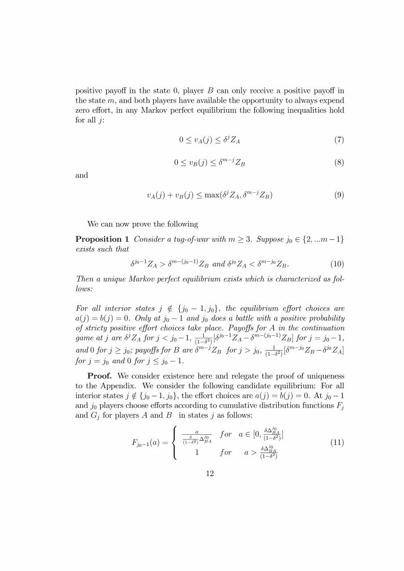
Proposition 1 Consider a tug-of-war with m ≥ 3. Suppose j0 ∈ {2, ...m−1}exists such that

δj0−1ZA > δm−(j0−1)ZB and δj0ZA < δm−j0ZB. (10)

Then a unique Markov perfect equilibrium exists which is characterized as fol-lows:

For all interior states j /∈ {j0 − 1, j0}, the equilibrium effort choices area(j) = b(j) = 0. Only at j0 − 1 and j0 does a battle with a positive probabilityof stricty positive effort choices take place. Payoffs for A in the continuationgame at j are δjZA for j < j0−1, 1

(1−δ2) [δj0−1ZA−δm−(j0−1)ZB] for j = j0−1,

and 0 for j ≥ j0; payoffs for B are δm−jZB for j > j0, 1(1−δ2) [δ

m−j0ZB−δj0ZA]

for j = j0 and 0 for j ≤ j0 − 1.Proof. We consider existence here and relegate the proof of uniqueness

to the Appendix. We consider the following candidate equilibrium: For allinterior states j /∈ {j0− 1, j0}, the effort choices are a(j) = b(j) = 0. At j0− 1and j0 players choose efforts according to cumulative distribution functions Fj

and Gj for players A and B in states j as follows:

Fj0−1(a) =

⎧⎪⎨⎪⎩a

δ(1−δ2)∆

j0BA

for a ∈ [0, δ∆j0BA

(1−δ2) ]

1 for a >δ∆

j0BA

(1−δ2)

(11)

12

Gj0−1(b) =

⎧⎨⎩ 1−δ

(1−δ2)∆j0BA

δδj0−2ZA+ b

δδj0−2ZAfor b ∈ [0, δ∆

j0BA

(1−δ2) ]

1 for b >δ∆

j0BA

(1−δ2)

(12)

Fj0(a) =

⎧⎨⎩ 1−δ

(1−δ2) ∆j0−1AB

δδm−(j0+1)ZB+ a

δδm−(j0+1)ZBfor a ∈ [0, δ ∆

j0−1AB

(1−δ2) ]

1 for a >δ ∆

j0−1AB

(1−δ2)

(13)

and

Gj0(b) =

⎧⎪⎨⎪⎩b

δ(1−δ2) ∆

j0−1AB

for b ∈ [0, δ ∆j0−1AB

(1−δ2) ]

1 for b >δ ∆

j0−1AB

(1−δ2) .(14)

where

∆j0BA = [δ

m−j0ZB − δj0ZA] and ∆j0−1AB = [δj0−1ZA − δm−(j0−1)ZB]. (15)

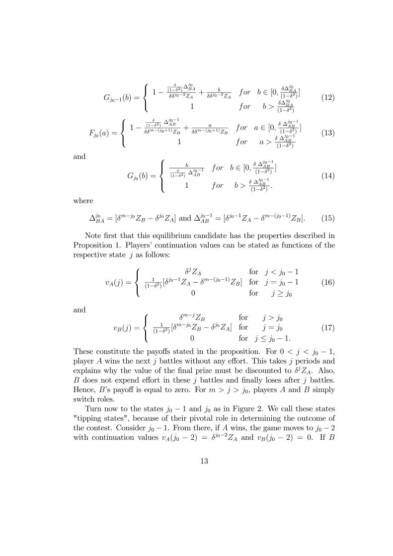
Note first that this equilibrium candidate has the properties described inProposition 1. Players’ continuation values can be stated as functions of therespective state j as follows:

vA(j) =

⎧⎨⎩δjZA for j < j0 − 1

1(1−δ2) [δ

j0−1ZA − δm−(j0−1)ZB] for j = j0 − 10 for j ≥ j0

(16)

and

vB(j) =

⎧⎨⎩δm−jZB for j > j0

1(1−δ2) [δ

m−j0ZB − δj0ZA] for j = j00 for j ≤ j0 − 1.

(17)

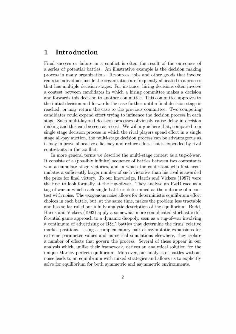
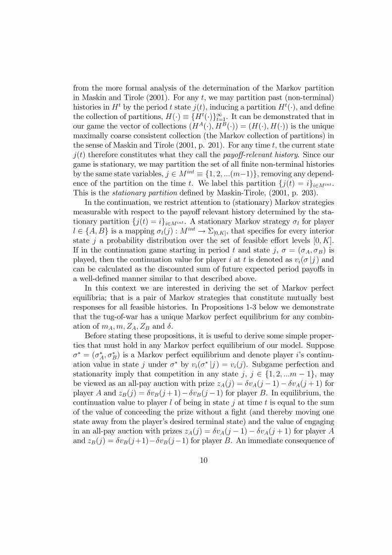
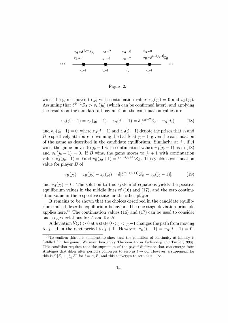
These constitute the payoffs stated in the proposition. For 0 < j < j0 − 1,player A wins the next j battles without any effort. This takes j periods andexplains why the value of the final prize must be discounted to δjZA. Also,B does not expend effort in these j battles and finally loses after j battles.Hence, B’s payoff is equal to zero. For m > j > j0, players A and B simplyswitch roles.Turn now to the states j0 − 1 and j0 as in Figure 2. We call these states

"tipping states", because of their pivotal role in determining the outcome ofthe contest. Consider j0− 1. From there, if A wins, the game moves to j0− 2with continuation values vA(j0 − 2) = δj0−2ZA and vB(j0 − 2) = 0. If B

13

... ...

AZjAv 20 −= δ

0=Bv

?=Av 0=Av( )

BZjmBv

Av1

0

0 +−=

=

δ0=Bv ?=Bv

20 −j 10 −j0

j 10 +j

Figure 2:

wins, the game moves to j0 with continuation values vA(j0) = 0 and vB(j0).Assuming that δj0−2ZA > vB(j0) (which can be confirmed later), and applyingthe results on the standard all-pay auction, the continuation values are

vA(j0 − 1) = zA(j0 − 1)− zB(j0 − 1) = δ[δj0−2ZA − vB(j0)] (18)

and vB(j0−1) = 0, where zA(j0−1) and zB(j0−1) denote the prizes that A andB respectively attribute to winning the battle at j0−1, given the continuationof the game as described in the candidate equilibrium. Similarly, at j0, if Awins, the game moves to j0 − 1 with continuation values vA(j0 − 1) as in (18)and vB(j0 − 1) = 0. If B wins, the game moves to j0 + 1 with continuationvalues vA(j0+1) = 0 and vB(j0+1) = δm−(j0+1)ZB. This yields a continuationvalue for player B of

vB(j0) = zB(j0)− zA(j0) = δ[δm−(j0+1)ZB − vA(j0 − 1)], (19)

and vA(j0) = 0. The solution to this system of equations yields the positiveequilibrium values in the middle lines of (16) and (17), and the zero continu-ation value in the respective state for the other player.It remains to be shown that the choices described in the candidate equilib-

rium indeed describe equilibrium behavior. The one-stage deviation principleapplies here.10 The continuation values (16) and (17) can be used to considerone-stage deviations for A and for B.A deviation b0(j) > 0 at a state 0 < j < j0−1 changes the path frommoving

to j − 1 in the next period to j + 1. However, vB(j − 1) = vB(j + 1) = 0 .

10To confirm this it is sufficient to show that the condition of continuity at infinity isfulfilled for this game. We may then apply Theorem 4.2 in Fudenberg and Tirole (1993).This condition requires that the supremum of the payoff difference that can emerge fromstrategies that differ after period t converges to zero as t → ∞. However, a supremum forthis is δt[Zi + 1

1−δK] for i = A,B, and this converges to zero as t→∞.

14

Hence, this deviation reduces B’s payoff by b0(j) compared to b(j) = 0. Adeviation b0(j) > 0 at j > j0 does not change the state in t + 1 compared tob(j) = 0 in the candidate equilibrium, due to the tiebreaking rule employed.The deviation reduces B’s payoff by b0(j) compared to b(j) = 0. An equivalentlogic applies for a(j) at states j /∈ {j0 − 1, j0}.Turn now to the state j0. In the candidate equilibrium, in state j0 contest-

ant A randomizes on the support [0, δ(1−δ2) [δ

j0−1ZA−δm−(j0−1)ZB]]. All actionsin the equilibrium support for A at j0 yield the same expected payoff equal toGj0(x)δvA(j0 − 1) + (1−Gj0(x))0− x = 0. A possible one-stage deviation forA at j0 is an a0(j0) > δ

(1−δ2) [δj0−1ZA − δm−(j0−1)ZB]. Compared to the action

a(j0) =δ

(1−δ2) [δj0−1ZA − δm−(j0−1)ZB] that is inside A’s equilibrium support,

this also leads to state j0−1, but costs the additional amount a0(j0)−a(j0) > 0.The deviation is therefore not profitable for A. The same type of argumentapplies for b(j0).A similar argument applies to the state j0−1. In the candidate equilibrium,

in state j0 − 1 contestant A randomizes on the support [0, δ(1−δ2)(δ

m−j0ZB −δj0ZA)]. All actions in the equilibrium support for A at j0 − 1 yield thesame expected payoff equal to Gj0−1(x)δvA(j0 − 2) + (1 − Gj0−1(x))0 − x =1

1−δ2 [δj0−1ZA − δm−(j0−1)ZB] = vA(j0 − 1).11 A possible one-stage deviation

for A at j0 − 1 is an a0(j0 − 1) > δ(1−δ2) [δ

m−j0ZB − δj0ZA]. Compared to the

action a(j0 − 1) = δ(1−δ2) [δ

m−j0ZB − δj0ZA] that is the upper bound of A’sequilibrium support, this also leads to state j0 − 2, but costs the additionalamount a0(j0 − 1)− a(j0 − 1) > 0. The deviation is not profitable for A. Thesame type of argument applies for b(j0 − 1).Intuitively, outside of the states j0−1 and j0, one of the players is indifferent

between winning and losing the component contest. For instance, in the statej0 − 2, the best that player B could achieve by winning the next componentcontest is to enter the state j0− 1 at which B’s continuation value is still zeroand smaller than player A’s continuation value. As B does not gain anythingfrom reaching j0− 1, B should not spend any effort trying to reach this state.But if B does not spend effort to win, it is easy for A to win.The states j0 − 1 and j0 are different. Battle victory or defeat at one of

these points leads to different continuation games and allocates a considerable

11More formally, all actions in the support of A’s equilibrium local strategy that are notmass points of B’s local strategy yield the same expected payoff. Since B has a mass pointat zero, this does not hold at a = 0, but for every a in a neigborhood above zero.

15

rent between A and B. This makes competition particularly strong at thesestates. We call these states "tipping states" because success of an advantagedplayer at each of these two states "tips" the game so that victory is obtainedwithout further effort. A loss by the advantaged player throws the systemback into a competitive state where the player becomes disadvantaged.Proposition 1 also shows that the allocation of a prize in a tug-of-war leads

to a seemingly peaceful outcome whenever the conflict starts in a state otherthan a tipping state. This will be important for drawing conclusions in section3 about the efficiency properties of a tug-of-war as an allocation mechanism.Proposition 1 does not consider all possible parameter cases. Before turning

to the remaining cases, note that the case j0 = 1 cannot emerge, as this requiresδZA < δm−1ZB, and this contradicts ZA ≥ ZB for m > 2. However, player A’sdominance could be sufficiently large that no interior j0 exists that has theproperties defined in Proposition 1. This leads to

Proposition 2 Suppose that δm−1ZA > δZB. Then a unique Markov perfectequilibrium exists with vB(j) = 0 and vA(j) = δjZA for all j ∈ {1, ...,m− 2},and vA(m− 1) = δm−1ZA − δZB and vB(m− 1) = 0 at j = m− 1.

Proof. We show that the following effort choices constitute an equilibriumand yield the payoffs described in the proposition. Uniqueness follows theargument in the Appendix.Effort is a(j) = b(j) = 0 for all j ∈M int\{m−1} and for j = m−1 efforts

are chosen according to the following cumulative distribution functions:

Fm−1(a) =½

aδZB

for a ∈ [0, δZB]

1 for a > δZB(20)

Gm−1(b) =½(1− δZB−b

δm−1ZA) for b ∈ [0, δZB]

1 for b > δZB.(21)

Note that this behavior yields the payoffs that are characterized in Proposition2. For states j = 1, 2, ..., (m − 2), A wins after j further battles, and noneof the players expends effort. This confirms vA(j) = δjZA and vB(j) = 0 forall j = 1, ...m − 2. For j = m, the payoffs are vA(m) = 0 and vB(m) = ZB.Finally, for j = m− 1, given the mixed strategies described by (20) and (21),the payoffs are vA(m− 1) = δm−1ZA > δZB and vB(m− 1) = 0.Now we confirm that the effort choices in the candidate equilibrium are

indeed mutually optimal replies. For interior states j < m − 1, a deviation

16

b0(j) > 0 makes B win the battle, instead of A. It leads to j + 1, instead ofj− 1, but vB(j+1) = vB(j− 1) = 0 . Hence, this deviation reduces B’s payoffby b0(j) compared to b(j) = 0. For A, for j < m − 1, contestant A reachesj = 0 along the shortest possible series of battle victories and does not spendany effort. Any positive effort can therefore only decrease A’s payoff. For j =m − 1, the battle either leads to j = m where B finally wins the prize, orto j = m − 2. The values the players attribute to reaching these states arevA(m) = 0, vB(m) = ZB, and vA(m− 2) = δm−2ZA and vB(m− 2) = 0. Usingthe results in Hillman and Riley (1989) and Baye, Kovenock and deVries (1996)on a complete information all-pay auction with prizes δ[δm−2ZA−0] = δm−1ZA

for A and δ[ZB−0] = δZB for B, it is confirmed that (20) and (21) describe theunique equilibrium cumulative distribution functions of effort for this all-payauction.Proposition 2 shows that a very strong player has a positive continuation

value regardless of the interior state in which the tug-of-war starts and winswith probability 1 without expending effort for every interior state exceptj = m− 1.So far we have ruled out the case of equality of continuation values at

interior states, and we turn to this case now which exhausts the set of possiblecases.

Proposition 3 The tug-of-war with δj0ZA = δ(m−j0)ZB ≡ Z for some j0 ∈{2, ...(m−1)} has a unique subgame perfect equilibrium in which players spenda(j) = b(j) = 0 in all interior states j 6= j0. They choose efforts a(j) and b(j)at j = j0 from the same uniform distribution on the range [0, Z]. Payoffs arevA(j) = δjZA and vB(j) = 0 for j < j0, vA(j) = 0 and vB(j) = δm−jZB forj > j0 and vA(j) = vB(j) = 0 for j = j0.

Proof. We again construct an equilibrium to demonstrate existence. Unique-ness follows from arguments similar to those appearing in the Appendix.In the candidate equilibrium each contestant expends zero effort at any

state j 6= j0 and expends effort at j = j0 according to a draw from thedistribution

F (x) =

½xZ

for x ∈ [0, Z]1 for x > Z.

(22)

At j = j0 the expected effort of each player equals Z/2, and each wins thisbattle with a probability of 1/2 and, in this case, eventually wins the overallcontest j0 − 1 or (m − j0) − 1 periods later, respectively, without spending

17

any further effort. This determines the continuation values in the candidateequilibrium. These continuation values are

vA = vB = 0 if j = j0vA = δjZA and vB = 0 if j < j0

vA = 0 and vB = δm−jZB if j > j0.(23)

It remains to show that the candidate equilibrium describes mutually op-timal replies. Consider one-stage deviations for A and B for some state j < j0.A choice a0(j) > 0 will not change the equilibrium outcome in the battle in thisperiod and hence will simply reduce A’s payoff by a0(j). A choice b0(j) > 0 willmake B win. If j < j0 − 1, following the candidate equilibrium A will simplywin a series of battles until final victory occurs. Hence, b0(j) > 0 reduces B’spayoff by this same amount b0(0) of effort. If j = j0−1, B’s battle victory willlead to j = j0, and candidate equilibrium play from here on will yield a payoffequal to zero to B. Accordingly, the deviation b0(j) > 0 yields a reductionof B’s payoff by this same amount. Consider one-stage deviations for A andB in some state j > j0. The same line of argument applies, with A and Bswitching roles. Finally, consider one-stage deviations for A and B at j = j0.Any such deviation for A must be a choice a0(j) > Z. Compared to a(j) = Z,this choice makes A win with the same probability 1, but yields a reductionin A’s payoff by a0(j)−Z, compared to a(j) = Z. The same argument appliesfor deviations by B at this state.The intuition for Proposition 3 is as follows. The two contestants enter into

a very strong fight whenever they reach the state j = j0. In this state theyare perfectly symmetric and they anticipate that the winner of the battle inthis state moves straight to final victory. In the battle that takes place in thiscase, they dissipate the maximum feasible rent from winning this battle. Thismaximum rent is what they get if they can move from there through a seriesof uncontested battles to final victory. Once one of the contestants, say A , hasacquired some advantage in the sense that the contest has moved to j < j0, theonly way for B to reach victory passes through the state with j = j0. As allrent is dissipated in the contest that takes place there, B is simply not willingto spend any effort to move the contest to that state. Hence, the considerableeffort that is spent at the point at which the tug-of-war becomes symmetricin terms of the prizes that are at stake for the two contestants prevents thecontestant who is lagging behind in terms of battle victories from spendingpositive effort.

18

Discounting played two important roles in our analysis. First, discountingleads to payoff functions that are continuous at infinity, allowing the applica-tion of the one-stage deviation principle, which greatly facilitates our proofs.Moreover, discounting is essential in giving a meaningful role to the distanceto the state with final victory. The following holds:

Proposition 4 For a given value of ZAZB

> 1, the tipping state j0 is an in-creasing step function of δ. Moreover, as δ → 1, A wins the tug-of-war withouteffort starting from any state j < m− 1.Proof. The tipping state j0 is by definition the smallest state j for which

player B is advantaged: j0 = min{j ∈M int¯̄δjZA ≤ δm−jZB } when this set is

non-empty, and j0 = m otherwise. For δ > 0, the inequality δjZA ≤ δm−jZB

is equivalent to δ2j−mZA ≤ ZB. Sincem ≥ 3, for δ sufficiently close to zero theinequality is clearly satisfied for j = m − 1, so that j0 is interior. Moreover,since δ2j−m ≥ 1 for j ≤ m

2, it must be the case that j0 > m

2. As δ → 1, the

inequality is violated at all interior states, even at j = m − 1. In this case,by definition j0 = m, and from Proposition 2 player A wins the war fromany state j < m − 1. For any 0 < δ < 1, δ2j−mZA ≤ ZB is equivalent to

2j − m ≥ logZBZA

log δ, so that j0 is the smallest index j satisfying the inequality.

Since the left hand side of this inequality is positive, and both the numeratorand denominator of the right hand side are negative, as δ increases, the righthand side monotonically increases, eventually diverging to∞ as δ → 1. Hence,as δ increases, the smallest index j satisfying the inequality must increase insteps until it hits m.As the discount factor increases, relative prize value or player strength

plays a greater role in the determination of the outcome than distance. Forany given value of ZB

ZA< 1, as δ increases the tipping state j0 moves in discrete

jumps towards m. Player A may suffer a greater distance disadvantage andstill win the prize with certainty.

3 Expenditure, allocative efficiency and thecost of delay

The tug-of-war with m > 2 resolves the allocation problem along a sequenceof states, where a violent battle may, but need not take place at each state.Only in the tipping states is positive effort expended with positive probability.

19

Once the process leaves the tipping states, the war moves to a terminal state,without further effort being expended. A tug-of-war that starts in a tippingstate will therefore be called "violent". A tug-of-war that starts outside atipping state will be called "peaceful".Compared to the standard all-pay auction, the tug-of-war could be inter-

preted as an institution that saves cost of effort in the problem of allocating aprize between rivals who are prepared to expend resources in fighting for theprize. Suppose for instance that ZA and ZB are independent random drawsfrom a continuous distribution with support [0, κ], where κ < K. Suppose thatthese values are known to the contestants but are not observable by the de-signer of the institution at the time that it must be implemented. Considerthe following tug-of-war as an anonymous mechanism in the case in which mis an even number, so that m

2is integer valued. Start the tug-of-war in the

symmetric state m2and assume, as we have throughout, that player A attempts

to move the state to j = 0 and player B attempts to move the state to j = m.Then the following result derives the probability of peaceful resolution:

Proposition 5 Let Γ(g) be the continuous cumulative distribution functionof g ≡ ZA/ZB, with support [0,∞]. The allocation is peaceful in the Markovperfect equilibrium with a probability Γ(δ2) + (1− Γ( 1

δ2)), and limδ→1(Γ(δ2) +

(1− Γ( 1δ2))) = 1.

Proof. For a proof we show that Γ(δ2)+(1−Γ( 1δ2)) is the probability that

the symmetric state m/2 is not a tipping state. Suppose that g > 1δ2. Then

ZA > ZB and δm2+1ZA > δm−(

m2+1)ZB. Hence, j0 − 1 > m

2. By Propositions

1-3 this implies that the tug-of-war that starts in m/2 consecutively moves toj = 0 with no effort being expended. Let g < δ2. Then ZA < ZB. Applyingthe results in Propositions 1-3 with A and B and j = 0 and j = m switchingroles shows that the tug-of-war that starts in m/2 moves to j = m withno effort being expended. Suppose now that g ∈ (1, 1

δ2). In this case j0 −

1 = m/2. Accordingly, a battle with positive expected efforts takes place atm/2 if δ

m2+1ZA 6= δm−(

m2+1)ZB. No expected effort is expended in this case

only if δm2+1ZA = δm−(

m2+1)ZB. However, the set of values of g for which

δm2+1ZA = δm−(

m2+1)ZB holds has a measure of zero. A similar argument

applies for g ∈ (δ2, 1), again with A and B and j = 0 and j = m switchingroles.Proposition 5 characterizes conditions on the asymmetry in the valuations

of the prize that are sufficient to make the tug-of-war evolve peacefully if it

20

starts in the symmetric state j = m/2. A sufficient condition for this to happenis that j = m

2is not a tipping state. If tipping states are j0 and j0 − 1 with

j0 − 1 > m/2 then the equilibrium process moves from j = m2further away

from the tipping states towards the terminal state j = 0. If ZA < ZB, and,hence, tipping states are j0 and j0+1, with j0+1 < m/2, then the equilibriumprocess moves further away from these states and towards the terminal statej = m.Note that the number of states is irrelevant for whether the tug-of-war

that starts in state j = m2is resolved peacefully or not, provided that m > 2.

Whether the tug-of-war is resolved peacefully or not depends only on the ratioof the two prizes and the discount factor. For a given continuous distributionof g, as the discount factor becomes large, the tug-of-war is resolved almostsurely peacefully.Of course, offsetting the potential gains from the tug-of-war in promoting

the peaceful resolution of resource contests are the potential costs of delayarising from the multi-stage nature of the conflict. The all-pay auction isresolved in a single stage (m = 2) and hence reduces this delay to the minimumattainable in a non-trivial contest. On the other hand, from Proposition 5 it isapparent that adding more states beyond m = 4 does not increase the chanceof peaceful resolution and only adds potential delay when a peaceful outcomearises. Moreover, if m

2is a tipping state, for a given draw of ZA and ZB the

sum of expected payoffs at this state is simply

δm/2

1− δ2max{(ZA − ZB), (ZB − ZA)} (24)

which is a strictly decreasing function in m. We state this as

Proposition 6 The sum of expected payoffs in the tug-of-war with m ≥ 4which have a symmetric state m

2is maximized at m = 4.

Using Proposition 5 we may compare the cases m = 2 and m = 4. Whenm = 4 we know that there is a probability Γ(δ2) + (1 − Γ(δ−2)) that theallocation is peaceful and a probability of Γ(δ−2)−Γ(δ2) that the allocation isviolent. We know that in the case m = 2 the allocation is always violent andthe sum of the players’ payoffs is δ(Z(1)−Z(2)), where Z(1) ≡ max(ZA, ZB) andZ(2) ≡ min(ZA, ZB). Ignoring discounting, the loss due to conflict, Z(2), can bedecomposed into the expected loss due to effort expended, 1

2Z(2)[1+(Z(2)/Z(1))],

21

and the expected loss due to misallocation of the prize, 12Z(2)[1− (Z(2)/Z(1))].

The loss due to delay then comes when the factor δ is applied.In the case where m = 4 the allocation is peaceful when (Z(1)/Z(2)) > δ−2.

In this case, starting from the state m2= 2 it takes two periods for the player

with the higher value to win and no effort is expended. Hence, the sum of thepayoffs of the two players in this case is δ2Z(1). The only inefficiency in thiscase is due to delay. For realizations of (ZA, ZB) satisfying (Z(1)/Z(2)) > δ−2,the tug-of-war is more efficient than the all-pay auction if and only if δ2Z(1) >δ(Z(1)−Z(2)) or, equivalently, (Z(1)/Z(2)) < (1− δ)−1. Since by assumption weare in the range where the tug-of-war is peaceful, (Z(1)/Z(2)) > δ−2. Note thatδ−2 > (1 − δ)−1 if δ < δ+ ≡

√5−12. In this case, the all-pay auction is more

efficient than the tug-of-war in this range of values of (Z(1)/Z(2)). For δ > δ+,δ−2 < (1 − δ)−1 and the tug-of-war is more efficient than the all-pay auctionfor values of (Z(1)/Z(2)) in the interval (δ

−2, (1− δ)−1) and the all-pay auctionis more efficient for values of (Z(1)/Z(2)) in the interval ((1− δ)−1,∞).When 1 ≤ (Z(1)/Z(2)) < δ−2, in the tug-of-war the state m

2is a tipping state

and the allocation involves active effort expenditure. The expected sum of thepayoffs in this case can again be compared to those in the all-pay auction. Form = 4 the expected sum of the payoffs in the tug-of-war can be calculatedfrom equation (24) and is equal to δ2

1−δ2 (Z(1) − Z(2)). Comparing this to theexpected sum of payoffs in the all-pay auction we find that for Z(1) 6= Z(2),δ2

1−δ2 (Z(1)−Z(2)) > δ(Z(1)−Z(2)) if and only if δ2+δ−1 > 0 or δ > δ+ ≡√5−12

.

Therefore, when the realization of (ZA, ZB) is such that the initial state m2

is a violent state in the tug-of-war, the tug-of-war is more efficient than theall-pay auction when δ > δ+ and the all-pay auction is more efficient than thetug-of-war when δ < δ+.We may summarize these results in the following proposition:

Proposition 7 When δ < δ+ =√5−12

, for any realization of (ZA, ZB), theall-pay auction (m = 2) is more efficient than a tug-of-war with m = 4. Whenδ > δ+ the tug-of-war with m = 4 is more efficient than the all-pay auctionfor (ZA, ZB) such that

Z(1)Z(2)∈ (1, (1 − δ)−1) and the all-pay auction is more

efficient for Z(1)Z(2)∈ ((1−δ)−1,∞). In particular, for any given continuous joint

distribution of (ZA, ZB), for sufficiently large δ the tug-or-war is more efficientthan the all-pay auction.

22

4 Conclusions

We studied the strategic behavior of players who compete in a series of singlebattles for two positive winner prizes. A sufficient lead in the number of battlevictories is needed to win the final prize. We showed that there is a uniquesubgame perfect equilibrium in Markov strategies and we characterized thisequilibrium. Contest effort concentrates on at most two states. Such states arecharacterized by three factors: the number of battle victories, or the ’distance’which the two contestants need to win the overall contest, the relative strengthor dominance of contestants, and the discount factor. The critical distancethat determines the tipping states in which the contest effort is focussed turnsout to be a function of the contestants’ relative strengths (or, equivalently, inthe relative valuations of the prize from final victory) and the discount factor.The larger one player’s dominance in strength, the higher must be this player’sdistance to final victory, compared to the other player’s distance.

Many animal species and economic institutions have developed mechan-isms such as hierarchies, or other organizational structures to govern the al-location of prizes, such as preferential food access and the right to reproducein the biological context, or prized jobs and contracts in the organizationalcontext. Behavior in these mechanisms could be interpreted as a conflict thatconsists of a series of battles, or repeated opportunities to struggle. Our resultshelp explain why these structures may have evolved. The tug-of-war delaysthe allocation of a given prize, compared to a single stage conflict, but canconsiderably increase the efficiency of allocation of the prize and reduce theoverall resources that are dissipated among the group of players.

5 Appendix

Consider a tug-of-war with m ≥ 3 and j0 ∈ {2, ...,m − 1} with the propertythat δj0ZA < δm−j0ZB and δj0−1ZA > δm−(j0−1)ZB. Then the Markov perfectequilibrium characterized in the Proposition 1 is unique in the class of Markovperfect equilibria.We will demonstrate the uniqueness of continuation values for every state j.

For given state-contingent continuation values we have already argued that theproblem reduces to a standard all-pay auction for both players at each interiorstate. Hence, uniqueness results from the uniqueness of the equilibrium in thestandard two-player all-pay auction with complete information.

23

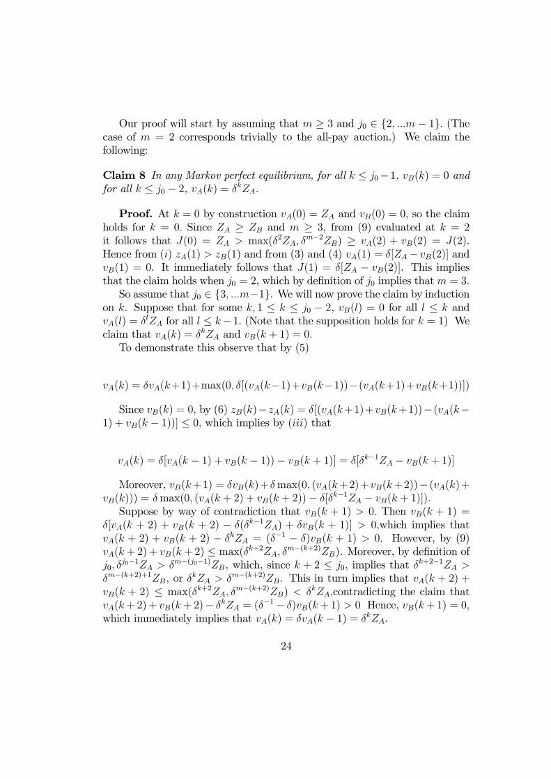
Our proof will start by assuming that m ≥ 3 and j0 ∈ {2, ...m− 1}. (Thecase of m = 2 corresponds trivially to the all-pay auction.) We claim thefollowing:

Claim 8 In any Markov perfect equilibrium, for all k ≤ j0−1, vB(k) = 0 andfor all k ≤ j0 − 2, vA(k) = δkZA.

Proof. At k = 0 by construction vA(0) = ZA and vB(0) = 0, so the claimholds for k = 0. Since ZA ≥ ZB and m ≥ 3, from (9) evaluated at k = 2it follows that J(0) = ZA > max(δ2ZA, δ

m−2ZB) ≥ vA(2) + vB(2) = J(2).Hence from (i) zA(1) > zB(1) and from (3) and (4) vA(1) = δ[ZA− vB(2)] andvB(1) = 0. It immediately follows that J(1) = δ[ZA − vB(2)]. This impliesthat the claim holds when j0 = 2, which by definition of j0 implies thatm = 3.So assume that j0 ∈ {3, ...m−1}. We will now prove the claim by induction

on k. Suppose that for some k, 1 ≤ k ≤ j0 − 2, vB(l) = 0 for all l ≤ k andvA(l) = δlZA for all l ≤ k− 1. (Note that the supposition holds for k = 1) Weclaim that vA(k) = δkZA and vB(k + 1) = 0.To demonstrate this observe that by (5)

vA(k) = δvA(k+1)+max(0, δ[(vA(k−1)+vB(k−1))−(vA(k+1)+vB(k+1))])

Since vB(k) = 0, by (6) zB(k)−zA(k) = δ[(vA(k+1)+vB(k+1))− (vA(k−1) + vB(k − 1))] ≤ 0, which implies by (iii) that

vA(k) = δ[vA(k − 1) + vB(k − 1))− vB(k + 1)] = δ[δk−1ZA − vB(k + 1)]

Moreover, vB(k+1) = δvB(k)+δmax(0, (vA(k+2)+vB(k+2))− (vA(k)+vB(k))) = δmax(0, (vA(k + 2) + vB(k + 2))− δ[δk−1ZA − vB(k + 1)]).Suppose by way of contradiction that vB(k + 1) > 0. Then vB(k + 1) =

δ[vA(k + 2) + vB(k + 2) − δ(δk−1ZA) + δvB(k + 1)] > 0,which implies thatvA(k + 2) + vB(k + 2) − δkZA = (δ−1 − δ)vB(k + 1) > 0. However, by (9)vA(k+ 2) + vB(k+2) ≤ max(δk+2ZA, δ

m−(k+2)ZB). Moreover, by definition ofj0, δ

j0−1ZA > δm−(j0−1)ZB, which, since k + 2 ≤ j0, implies that δk+2−1ZA >

δm−(k+2)+1ZB, or δkZA > δm−(k+2)ZB. This in turn implies that vA(k + 2) +

vB(k + 2) ≤ max(δk+2ZA, δm−(k+2)ZB) < δkZA,contradicting the claim that

vA(k+2)+ vB(k+2)− δkZA = (δ−1− δ)vB(k+1) > 0 Hence, vB(k+1) = 0,

which immediately implies that vA(k) = δvA(k − 1) = δkZA.

24

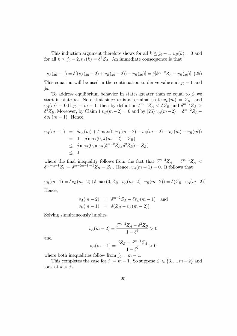
This induction argument therefore shows for all k ≤ j0− 1, vB(k) = 0 andfor all k ≤ j0 − 2, vA(k) = δkZA. An immediate consequence is that

vA(j0 − 1) = δ[(vA(j0 − 2) + vB(j0 − 2))− vB(j0)] = δ[δj0−2ZA− vB(j0)] (25)

This equation will be used in the continuation to derive values at j0 − 1 andj0.To address equilibrium behavior in states greater than or equal to j0,we

start in state m. Note that since m is a terminal state vB(m) = ZB andvA(m) = 0.If j0 = m − 1, then by definition δm−1ZA < δZB and δm−2ZA >δ2ZB.Moreover, by Claim 1 vB(m−2) = 0 and by (25) vA(m−2) = δm−2ZA−δvB(m− 1). Hence,

vA(m− 1) = δvA(m) + δmax(0, vA(m− 2) + vB(m− 2)− vA(m)− vB(m))

= 0 + δmax(0, J(m− 2)− ZB)

≤ δmax(0,max(δm−2ZA, δ2ZB)− ZB)

≤ 0

where the final inequality follows from the fact that δm−2ZA = δj0−1ZA <δm−j0−1ZB = δm−(m−1)−1ZB = ZB. Hence, vA(m− 1) = 0. It follows that

vB(m−1) = δvB(m−2)+δmax(0, ZB−vA(m−2)−vB(m−2)) = δ(ZB−vA(m−2))Hence,

vA(m− 2) = δm−2ZA − δvB(m− 1) and

vB(m− 1) = δ(ZB − vA(m− 2))Solving simultaneously implies

vA(m− 2) = δm−2ZA − δ2ZB

1− δ2> 0

and

vB(m− 1) = δZB − δm−1ZA

1− δ2> 0

where both inequalities follow from j0 = m− 1.This completes the case for j0 = m− 1. So suppose j0 ∈ {3, ...,m− 2} and

look at k > j0.

25

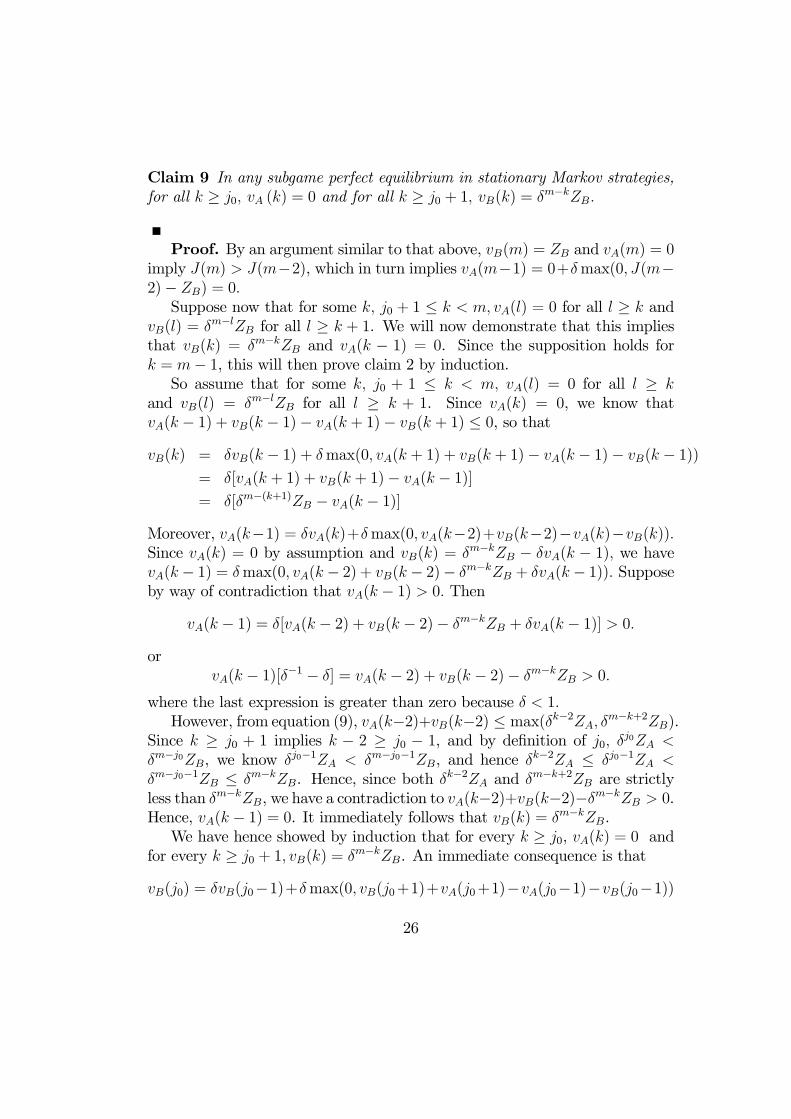
Claim 9 In any subgame perfect equilibrium in stationary Markov strategies,for all k ≥ j0, vA (k) = 0 and for all k ≥ j0 + 1, vB(k) = δm−kZB.

Proof. By an argument similar to that above, vB(m) = ZB and vA(m) = 0imply J(m) > J(m−2), which in turn implies vA(m−1) = 0+δmax(0, J(m−2)− ZB) = 0.Suppose now that for some k, j0 + 1 ≤ k < m, vA(l) = 0 for all l ≥ k and

vB(l) = δm−lZB for all l ≥ k + 1. We will now demonstrate that this impliesthat vB(k) = δm−kZB and vA(k − 1) = 0. Since the supposition holds fork = m− 1, this will then prove claim 2 by induction.So assume that for some k, j0 + 1 ≤ k < m, vA(l) = 0 for all l ≥ k

and vB(l) = δm−lZB for all l ≥ k + 1. Since vA(k) = 0, we know thatvA(k − 1) + vB(k − 1)− vA(k + 1)− vB(k + 1) ≤ 0, so thatvB(k) = δvB(k − 1) + δmax(0, vA(k + 1) + vB(k + 1)− vA(k − 1)− vB(k − 1))

= δ[vA(k + 1) + vB(k + 1)− vA(k − 1)]= δ[δm−(k+1)ZB − vA(k − 1)]

Moreover, vA(k−1) = δvA(k)+δmax(0, vA(k−2)+vB(k−2)−vA(k)−vB(k)).Since vA(k) = 0 by assumption and vB(k) = δm−kZB − δvA(k − 1), we havevA(k − 1) = δmax(0, vA(k − 2) + vB(k − 2)− δm−kZB + δvA(k − 1)). Supposeby way of contradiction that vA(k − 1) > 0. Then

vA(k − 1) = δ[vA(k − 2) + vB(k − 2)− δm−kZB + δvA(k − 1)] > 0.or

vA(k − 1)[δ−1 − δ] = vA(k − 2) + vB(k − 2)− δm−kZB > 0.

where the last expression is greater than zero because δ < 1.However, from equation (9), vA(k−2)+vB(k−2) ≤ max(δk−2ZA, δ

m−k+2ZB).Since k ≥ j0 + 1 implies k − 2 ≥ j0 − 1, and by definition of j0, δj0ZA <δm−j0ZB, we know δj0−1ZA < δm−j0−1ZB, and hence δk−2ZA ≤ δj0−1ZA <δm−j0−1ZB ≤ δm−kZB. Hence, since both δk−2ZA and δm−k+2ZB are strictlyless than δm−kZB, we have a contradiction to vA(k−2)+vB(k−2)−δm−kZB > 0.Hence, vA(k − 1) = 0. It immediately follows that vB(k) = δm−kZB.We have hence showed by induction that for every k ≥ j0, vA(k) = 0 and

for every k ≥ j0 + 1, vB(k) = δm−kZB. An immediate consequence is that

vB(j0) = δvB(j0−1)+δmax(0, vB(j0+1)+vA(j0+1)−vA(j0−1)−vB(j0−1))

26

Since vA(j0) = 0 implies J(j0 − 1) − J(j0 + 1) ≤ 0, the maximand in theexpression is nonnegative and

(7) vB(j0) = δ[vB(j0 + 1) + vA(j0 + 1)− vA(j0 − 1)]= δ[δm−(j0+1)ZB − vA(j0 − 1)]

Since from (25) vA(j0 − 1) = δ[δj0−2ZA − vB(j0)], we have a system of twolinearly independent equations in two unknowns. These have a unique solutionwhich is

vA(j0 − 1) =δj0−1ZA − δm−j0+1ZB

1− δ2> 0

vB(j0) =δm−j0ZB − δj0ZA

1− δ2> 0

6 References

Amann, E. and W. Leininger, 1995, Expected revenue of all-pay and first-pricesealed bid auctions with affiliated signals, Journal of Ecnomics - Zeitschrift fürNationalökonomie 61 (3), 273-279Amann, E. and W. Leininger, 1996, Asymmetric all-pay auctions with

incomplete information: The two-player case, Games and Ecnomic Behavior,14 (1), 1-18.Arbatskaya, M., 2003, The exclusion principle for symmetric multi-prize

all-pay auctions with endogenous valuations, Economics Letters, 80 (1), 73-80.Baik, K.H., I.G. Kim and S.Y. Na, 2001, Bidding for a group-specific

public-good prize, Journal of Public Economics, 82 (3), 415-429.Baye, M.R., D. Kovenock, and C. de Vries, 1993, Rigging the lobbying

process: an application of the all-pay auction, American Economic Review,83(1), 289-294.Baye, M.R., D. Kovenock, and C. de Vries, 1996, The all-pay auction with

complete information, Economic Theory, 8(2), 291-305.Baye, M.R., D. Kovenock, and de Vries, 2005, Comparative analysis of

litigation systems: an auction-theoretic approach, Economic Journal (forth-coming).

27

Beacham, J.L., 2003, Models of dominance hierarchy formation: Effects ofprior experience and intrinsic traits, Behaviour, 140, 1275-1303 Part 10Bergman, D.A., C. Kozlowski, J.C. McIntyre, R. Huber, A.G. Daws and

P.A. Moore, 2003, Temporal dynamics and communication of winner-effectsin the crayfish, orconectes rusticus, Behaviour, 140, 805-825 Part 6.Budd, C., C. Harris and J. Vickers, 1993, A model of the evolution of

duopoly: does the asymmetry between firms tend to increase or decrease?Review of Economic Studies, 60(3), 543-573.Che, Y.K., and I. Gale, 1998, Caps on political lobbying, American Eco-

nomic Review, 88, 643-651.Che, Y.K., and I. Gale, 2003, Optimal design of research contests, Amer-

ican Economic Review, 93 (3), 646-671.Ehrenberg, M. and J.L. McGrath, 2004, Actin mobility: staying on track

takes a little more effort, Current Biology, 14(21), R931-R932.Ellingsen, T., 1991, Strategic buyers and the social cost of monopoly, Amer-

ican Economic Review, 81(3), 648-657.Fudenberg, D., and J. Tirole, 1993, Game Theory, MIT Press, Cambridge

MA.Gavious, A., B. Moldovanu and A. Sela, 2002, Bid costs and endogenous

bid caps, RAND Journal of Economics, 33 (4), 709-722.Hammerstein, P., 1981, The role of asymmetries in animal contests, Animal

Behavior, 29, 193-205.Harris, C., and J. Vickers, 1987, Racing with uncertainty, Review of Eco-

nomic Studies, 54(1), 1-21.Hemelrijk, C.K., 2000, Towards the integration of social dominance and

spatial structure, Animal Behaviour, 59, Part 5, 1035-1048.Hillman, A., and J.G. Riley, 1989, Politically contestable rents and trans-

fers, Economics and Politics, 1, 17-40.Hsu, Y.Y. and L.L. Wolf, 1999, The winner and loser effect: integrating

multiple experiences, Animal Behaviour, 57, Part 4, 903-910.Kaplan, T.R., I. Luski, and D. Wettstein, 2003, Innovative activity and

sunk cost, International Journal of Industrial Organization, 21(8), 1111-1133.Konrad, K.A., 2004, Inverse Campaigning, Economic Journal, 114 (492),

69-82.Krishna, V., and J. Morgan, 1997, An analysis of the war of attrition and

the all-pay auction, Journal of Economic Theory, 72 (2), 343-362.Kura, T., 1999, Dilemma of the equality: an all-pay contest with individual

differences in resource holding potential, Journal of Theoretical Biology, 198

28

(3), 395-404.Larsson, M., Beignon, A.S., and Bhardway, N., 2004, DC-virus interplay:

a double edged sword, Seminars in Immunology, 16(3), 147-161.Maskin, E. and J. Tirole, 2001, Markov perfect equilibrium I. Observable

actions, Journal of Economic Theory, 100(2), 191-219.McAfee, R. Preston, 2000, Continuing wars of attrition, unpublished ma-

nuscript.Moldovanu, B. and A. Sela, 2001, The optimal allocation of prizes in con-

tests, American Economic Review, 91 (3), 542-558.Moldovanu, B. and A. Sela, 2004, Contest architecture, Journal of Eco-

nomic Theory (forthcoming).Müller, H.M., and K. Wärneryd, 2001, Inside versus outside ownership: a

political theory of the firm, RAND Journal of Economics, 32(3), 527-541.Organski, A.F.K., and E. Lust-Okar, 1997, The tug of war over the status

of Jerusalem: Leaders, strategies and outcomes, International Interactions, 23n(3-4), 333-350.Parker, G.A., and D.I. Rubenstein, 1981, Role assessment, reserve strategy,

and acquisition of information in asymmetric animal conflicts, Animal Beha-vior 29, 221-240.Radner, R., 1992, Hierarchy: the economics of managing, Journal of Eco-

nomic Literature, 30 (3), 1382-1415.Radner, R.,1993, The organization of decentralized information processing,

Econometrica, 61 (5), 1109-1146.Runciman, S., 1987, A History of the Crusades, Cambridge University

Press, Cambridge.Sahuguet, N. and N. Persico, 2005, Campaign spending regulation in a

model of redistributive politics, Economic Theory (forthcoming).Schaub, H., 1995, Dominance fades with distance - an experiment on food

competition in long-tailed macaques (macaca fascicularis), Journal of Com-parative Psychology, 109(2), 196-202.Tibbetts, E.A., and H.K. Reeve, 2000, Aggression and resource sharing

among foundresses in social wasp Polistes dominulus, Behavioral Ecology andSociobiology, 48(5), 344-352.Wärneryd, K., 1998, Distributional conflict and jurisdictional organization,

Journal of Public Economics, 69, 435-450.Whitford, A.B., 2005, The pursuit of political control by multiple prin-

cipals, Journal of Politics, 67(1), 29-49.

29

Yoo, C.Y., 2001, The Bush administration and the prospects of US-NorthKorean relations, Korean Journal of Defense Analysis, 13(1), 129-152.Zhou, D.P., C. Cantu, Y. Sagiv, N. Schrantz, A.B. Kulkarni, X.Y. Qi, D.J.

Mahuran, C.R. Morales, G.A. Grabowski, K. Benlagha, P. Savage, A. Bendelacand L. Teyton, 2004, Editing of CD1d-bound lipid antigens by endosomal lipidtransfer proteins, Science, 303 (5657), 523-527.

30