Embed Size (px)
Citation preview

P O L Y M E R P R O C E S S M O D E L I N G
3
AspenTech7
Vers
ion
V O L U M E 2
Use r G u i de
With Aspen Plus 107
Polymers Plus 7
COPYRIGHT 1981—1999 Aspen Technology, Inc.ALL RIGHTS RESERVED
The flowsheet graphics and plot components of Aspen Plus were developed by MY-Tech, Inc.
Aspen Aerotran�� Aspen Pinch�� ADVENT®� Aspen B-JAC�� Aspen Custom Modeler�� Aspen
Dynamics�� Aspen Hetran�� Aspen Plus®, AspenTech®, B-JAC®� BioProcess Simulator (BPS)�,
DynaPlus�, ModelManager�, Plantelligence�, the Plantelligence logo�, Polymers Plus®, PropertiesPlus®, SPEEDUP®, and the aspen leaf logo� are either registered trademarks, or trademarks of AspenTechnology, Inc., in the United States and/or other countries.
BATCHFRAC� and RATEFRAC� are trademarks of Koch Engineering Company, Inc.
Activator is a trademark of Software Security, Inc.
Rainbow SentinelSuperPro� is a trademark of Rainbow Technologies, Inc.
Élan License Manager is a trademark of Élan Computer Group, Inc., Mountain View, California, USA.
Microsoft Windows, Windows NT, Windows 95 and Windows 98 are either registered trademarks ortrademarks of Microsoft Corporation in the United States and/or other countries.
All other brand and product names are trademarks or registered trademarks of their respectivecompanies.
The License Manager portion of this product is based on:
Élan License Manager© 1989-1997 Élan Computer Group, Inc.All rights reserved
Use of Aspen Plus and This ManualThis manual is intended as a guide to using Aspen Plus process modeling software. This documentation containsAspenTech proprietary and confidential information and may not be disclosed, used, or copied without the priorconsent of AspenTech or as set forth in the applicable license agreement. Users are solely responsible for theproper use of Aspen Plus and the application of the results obtained.
Although AspenTech has tested the software and reviewed the documentation, the sole warranty for Aspen Plusmay be found in the applicable license agreement between AspenTech and the user. ASPENTECH MAKES NOWARRANTY OR REPRESENTATION, EITHER EXPRESS OR IMPLIED, WITH RESPECT TO THISDOCUMENTATION, ITS QUALITY, PERFORMANCE, MERCHANTABILITY, OR FITNESS FOR APARTICULAR PURPOSE.
Polymers Plus User Guide vii
CONTENTS
VOLUME 1Chapter 1 Introduction
About Polymers Plus................................................................................................. 1•1Overview of Polymerization Processes .................................................................... 1•2
Polymer Manufacturing Process Steps ................................................................. 1•2Issues of Concern in Polymer Process Modeling..................................................... 1•4
Monomer Synthesis and Purification.................................................................... 1•5Polymerization........................................................................................................ 1•5Recovery / Separation ............................................................................................ 1•6Polymer Processing ................................................................................................ 1•6Summary................................................................................................................. 1•6
Polymers Plus Tools.................................................................................................. 1•7Component Characterization................................................................................. 1•7Polymer Physical Properties.................................................................................. 1•8Polymerization Kinetics......................................................................................... 1•8Modeling Data ........................................................................................................ 1•8Process Flowsheeting ............................................................................................. 1•9
Defining a Model in Polymers Plus........................................................................ 1•10References ............................................................................................................... 1•12
Chapter 2 Polymer Structural Characterization
Polymer Structure..................................................................................................... 2•2Polymer Structural Properties................................................................................. 2•5Characterization Approach ...................................................................................... 2•5
Component Attributes............................................................................................ 2•6References ................................................................................................................. 2•6
Section 2.1 Component Classification
Component Categories.............................................................................................. 2•7Conventional Components..................................................................................... 2•8Polymers ................................................................................................................. 2•9Oligomers................................................................................................................ 2•9Segments............................................................................................................... 2•10Site-Based ............................................................................................................. 2•10
Component Databanks ........................................................................................... 2•11Pure Component Databank ................................................................................. 2•11Segment Databank............................................................................................... 2•12Polymer Databank................................................................................................ 2•12
Segment Methodology..............................................................................................2-13
CONTENTS
viii
Specifying Components...........................................................................................2•13Selecting Databanks.............................................................................................2•14Defining Component Names and Types..............................................................2•14Specifying Segments.............................................................................................2•15Specifying Polymers .............................................................................................2•15Specifying Oligomers............................................................................................2•16Specifying Site-Based Components .....................................................................2•17
References................................................................................................................2•18
Section 2.2 Polymer Structural Properties
Structural Properties as Component Attributes ...................................................2•19Component Attribute Classes.................................................................................2•20Component Attribute Categories ...........................................................................2•21
Polymer Component Attributes...........................................................................2•21Site-Based Species Attributes..............................................................................2•32User Attributes .....................................................................................................2•33
Component Attribute Initialization .......................................................................2•34Attribute Initialization Scheme...........................................................................2•34
Specifying Component Attributes ..........................................................................2•39Specifying Polymer Component Attributes ........................................................2•39Specifying Site-Based Component Attributes ....................................................2•39Specifying Conventional Component Attributes ................................................2•39Initializing Component Attributes in Streams or Blocks ..................................2•40
References................................................................................................................2•40
Section 2.3 Structural Property Distributions
Property Distribution Types...................................................................................2•41Distribution Functions............................................................................................2•43
Schulz-Flory Most Probable Distribution ...........................................................2•43Stockmayer Bivariate Distribution .....................................................................2•44
Distributions in Process Models.............................................................................2•45Average Properties and Moments .......................................................................2•45Method of Instantaneous Properties ...................................................................2•47Co-polymerization.................................................................................................2•50
Mechanism for Tracking Distributions..................................................................2•51Distributions in Kinetic Reactors ........................................................................2•51Distributions in Process Streams ........................................................................2•53
Requesting Distribution Calculations....................................................................2•54Selecting Distribution Characteristics ................................................................2•54Displaying Distribution Data for a Reactor........................................................2•54Displaying Distribution Data for Streams..........................................................2•55
References................................................................................................................2•56
Polymers Plus User Guide ix
Section 2.4 End-Use Properties
Polymer Properties ................................................................................................. 2•59End-Use Properties................................................................................................. 2•60
Relationship to Molecular Structure................................................................... 2•60Method for Calculating End-Use Properties ......................................................... 2•62
Intrinsic Viscosity................................................................................................. 2•63Zero-Shear Viscosity ............................................................................................ 2•63Density of Copolymer........................................................................................... 2•64Melt Index............................................................................................................. 2•64Melt Index Ratio................................................................................................... 2•65
Calculating End-Use Properties ............................................................................ 2•65Selecting an End-Use Property ........................................................................... 2•65Adding an End-Use Property Prop-Set............................................................... 2•66
References ............................................................................................................... 2•67
Chapter 3 Thermodynamic Properties
Properties of Interest in Process Simulation .......................................................... 3•2Properties for Equilibrium, Mass and Energy Balances ..................................... 3•2Properties for Detailed Equipment Design........................................................... 3•3Summary of Important Properties for Modeling.................................................. 3•3
Differences Between Polymers and Non-polymers................................................. 3•4Modeling Phase Equilibria in Polymer-Containing Mixtures................................ 3•6Modeling Other Thermophysical Properties of Polymers .................................... 3•10Property Models Available in Polymers Plus........................................................ 3•11
Activity Coefficient Models .................................................................................. 3•12Equations-of-State................................................................................................ 3•13Other Thermophysical Models ............................................................................ 3•14
Property Methods.................................................................................................... 3•15Thermodynamic Data for Polymers....................................................................... 3•17References ............................................................................................................... 3•18
Section 3.1 Van Krevelen Property Models
Summary of Applicability....................................................................................... 3•21Van Krevelen Models.............................................................................................. 3•22Liquid Enthalpy Model........................................................................................... 3•23
Liquid Enthalpy Model Parameters.................................................................... 3•24Solid Enthalpy Model ............................................................................................. 3•26
Solid Enthalpy Model Parameters ...................................................................... 3•27Liquid Gibbs Free Energy Model ........................................................................... 3•29
Liquid Gibbs Free Energy Model Parameters.................................................... 3•30Solid Gibbs Free Energy Model.............................................................................. 3•32
Solid Gibbs Free Energy Model Parameters ...................................................... 3•33Liquid Molar Volume Model................................................................................... 3•35
Liquid Molar Volume Model Parameters............................................................ 3•37Solid Molar Volume Model ..................................................................................... 3•38
Solid Molar Volume Model Parameters .............................................................. 3•39
CONTENTS
x
Glass Transition Temperature Correlation...........................................................3•41Glass Transition Correlation Parameters...........................................................3•41
Melt Transition Temperature Correlation ............................................................3•42Melt Transition Model Parameters .....................................................................3•42
Van Krevelen Property Parameter Estimation.....................................................3•43Specifying Physical Properties ...............................................................................3•44
Selecting Physical Property Methods..................................................................3•44Creating Customized Physical Property Methods..............................................3•45Entering Parameters for a Physical Property Model .........................................3•46Entering a Physical Property Parameter Estimation Method ..........................3•47Entering Molecular Structure for a Physical Property Estimation ..................3•48Entering Data for Physical Properties Parameter Optimization ......................3•49
References................................................................................................................3•50
Section 3.2 Tait Molar Volume Model
Summary of Applicability .......................................................................................3•51Tait Molar Volume Model .......................................................................................3•52
Tait Model Parameters.........................................................................................3•53Specifying the Tait Molar Volume Model ..............................................................3•53References................................................................................................................3•54
Section 3.3 Polymer Viscosity Models
Summary of Applicability .......................................................................................3•55Pure Polymer Modified Mark-Houwink Model .....................................................3•56
Modified Mark-Houwink Model Parameters ......................................................3•58Van Krevelen Viscosity-Temperature Correlation.............................................3•59Van Krevelen Correlation Parameters................................................................3•63
Concentrated Polymer Solution Viscosity Model ..................................................3•64Quasi-Binary System ...........................................................................................3•64Properties of Pseudo-Components.......................................................................3•65Solution Viscosity Model Parameters..................................................................3•67Polymer Solution Viscosity Estimation...............................................................3•67Polymer Solution Glass Transition Temperature ..............................................3•69Polymer Viscosity At Mixture Glass Transition Temperature ..........................3•69True Solvent Dilution Effect................................................................................3•70
Specifying the Viscosity Models .............................................................................3•70References................................................................................................................3•71
Section 3.4 Flory-Huggins Activity Coefficient Model
Summary of Applicability .......................................................................................3•73Flory-Huggins Model ..............................................................................................3•74
Flory-Huggins Model Parameters .......................................................................3•77Specifying the Flory-Huggins Model......................................................................3•77References................................................................................................................3•78
Polymers Plus User Guide xi
Section 3.5 NRTL Activity Coefficient Models
Summary of Applicability....................................................................................... 3•79Polymer NRTL Model Overview ............................................................................ 3•80Polymer NRTL Model ............................................................................................. 3•81Random Copolymer NRTL Model .......................................................................... 3•83
Parameters for the NRTL Models ....................................................................... 3•85Comparisons of the Polymer NRTL Models .......................................................... 3•86
Similarities ........................................................................................................... 3•86Differences ............................................................................................................ 3•86
Specifying the Polymer NRTL Models................................................................... 3•86References ............................................................................................................... 3•87
Section 3.6 UNIFAC Activity Coefficient Model
Summary of Applicability....................................................................................... 3•89Polymer UNIFAC Model ........................................................................................ 3•90
Polymer UNIFAC Model Parameters ................................................................. 3•92Specifying the UNIFAC Model............................................................................... 3•92References ............................................................................................................... 3•93
Section 3.7 Polymer UNIFAC Free Volume Model
Summary of Applicability....................................................................................... 3•95Polymer UNIFAC Free Volume Model .................................................................. 3•96
Polymer UNIFAC Free Volume Model Parameters........................................... 3•97Specifying the Polymer UNIFAC Free Volume Model ......................................... 3•97References ............................................................................................................... 3•98
Section 3.8 Polymer Ideal Gas Property Model
Summary of Applicability....................................................................................... 3•99Polymer Ideal Gas Property Model...................................................................... 3•100
Polymer Ideal Gas Model Parameters .............................................................. 3•102Specifying the Ideal Gas Model............................................................................ 3•102References ............................................................................................................. 3•103
Section 3.9 Sanchez-Lacombe EOS Model
Summary of Applicability..................................................................................... 3•105Sanchez-Lacombe Model ...................................................................................... 3•108
Pure Fluids ......................................................................................................... 3•108Fluid Mixtures.................................................................................................... 3•110Polymer Systems ................................................................................................ 3•111Sanchez-Lacombe Model Parameters ............................................................... 3•112
Specifying the Sanchez-Lacombe EOS Model ..................................................... 3•112References ............................................................................................................. 3•113
CONTENTS
xii
Section 3.10 Polymer SRK EOS Model
Summary of Applicability .....................................................................................3•116Polymer SRK EOS Model .....................................................................................3•117
Polymer SRK EOS Model Parameters ..............................................................3•119Specifying the Polymer SRK EOS Model ............................................................3•122References..............................................................................................................3•122
Section 3.11 SAFT Equation-of-State Model
Summary of Applicability .....................................................................................3•123SAFT EOS Model ..................................................................................................3•124
Extension to Fluid Mixtures ..............................................................................3•128Application of SAFT..............................................................................................3•130
SAFT EOS Model Parameters ...........................................................................3•132Specifying the SAFT EOS Model .........................................................................3•132References..............................................................................................................3•133
Chapter 4 Polymerization Reactions
Polymerization Reaction Categories ........................................................................4•2Step-Growth Polymerization .................................................................................4•4Chain-Growth Polymerization...............................................................................4•5
Polymerization Process Types ..................................................................................4•6Polymers Plus Reaction Models ...............................................................................4•7
Built-in Models .......................................................................................................4•7User Models ............................................................................................................4•8
References..................................................................................................................4•9
Section 4.1 Step-Growth Polymerization Model
Summary of Applications .......................................................................................4•12Step-Growth Processes ...........................................................................................4•12
Polyesters ..............................................................................................................4•12Nylon-6 ..................................................................................................................4•19Nylon-6,6 ...............................................................................................................4•20Polycarbonate .......................................................................................................4•23
Reaction Kinetic Scheme ........................................................................................4•25Overview ...............................................................................................................4•25Polyester Reaction Kinetics .................................................................................4•30Nylon-6 Reaction Kinetics....................................................................................4•37Nylon-6,6 Reaction Kinetics.................................................................................4•41Melt Polycarbonate Reaction Kinetics ................................................................4•49
Model Features and Assumptions..........................................................................4•52Model Predictions .................................................................................................4•52Phase Equilibria ...................................................................................................4•52Reaction Mechanism ............................................................................................4•53
Model Structure ......................................................................................................4•53Reacting Groups and Species...............................................................................4•53Reaction Stoichiometry Generation ....................................................................4•60Model-Generated Reactions.................................................................................4•61
Polymers Plus User Guide xiii
User Reactions...................................................................................................... 4•67User Subroutines.................................................................................................. 4•69
Specifying Step-Growth Polymerization Kinetics................................................. 4•87Accessing the Step-Growth Model....................................................................... 4•87Specifying the Step-Growth Model ..................................................................... 4•88Specifying Reacting Components ........................................................................ 4•89Listing Built-In Reactions.................................................................................... 4•89Specifying Built-In Reaction Rate Constants..................................................... 4•90Assigning Rate Constants to Reactions .............................................................. 4•90Including User Reactions..................................................................................... 4•91Adding or Editing User Reactions....................................................................... 4•92Assigning Rate Constants to User Reactions ..................................................... 4•92Selecting Report Options ..................................................................................... 4•92Including a User Kinetic Subroutine .................................................................. 4•93Including a User Rate Constant Subroutine ...................................................... 4•93Including a User Basis Subroutine ..................................................................... 4•93
References ............................................................................................................... 4•94
Section 4.2 Free-Radical Bulk Polymerization
Summary of Applications ....................................................................................... 4•96Free-Radical Bulk/Solution Processes ................................................................... 4•97Reaction Kinetic Scheme........................................................................................ 4•97
Initiation ............................................................................................................. 4•102Propagation......................................................................................................... 4•104Chain Transfer to Small Molecules................................................................... 4•105Termination ........................................................................................................ 4•105Short and Long Chain Branching ..................................................................... 4•106Beta-Scission....................................................................................................... 4•107
Model Features and Assumptions........................................................................ 4•107Calculation Method ............................................................................................ 4•108Quasi-Steady-State Approximation (QSSA)..................................................... 4•109Phase Equilibrium.............................................................................................. 4•109Gel Effect ............................................................................................................ 4•109
Polymer Properties Calculated ............................................................................ 4•112Specifying Free-Radical Polymerization Kinetics............................................... 4•115
Accessing the Free-Radical Model..................................................................... 4•115Specifying the Free-Radical Model.................................................................... 4•115Specifying Reacting Species............................................................................... 4•116Listing Reactions................................................................................................ 4•116Adding Reactions................................................................................................ 4•117Editing Reactions ............................................................................................... 4•117Assigning Rate Constants to Reactions ............................................................ 4•118Selecting Calculation Options ........................................................................... 4•118Adding Gel-Effect ............................................................................................... 4•118
References ............................................................................................................. 4•119
CONTENTS
xiv
Section 4.3 Emulsion Polymerization Model
Summary of Applications .....................................................................................4•122Emulsion Polymerization Processes ....................................................................4•123Reaction Kinetic Scheme ......................................................................................4•123
Micellar Nucleation ............................................................................................4•124Homogeneous Nucleation...................................................................................4•128Particle Growth ..................................................................................................4•130Radical Balance ..................................................................................................4•131Kinetics of Emulsion Polymerization ................................................................4•136
Model Features and Assumptions........................................................................4•139Model Assumptions ............................................................................................4•139Thermodynamics of Monomer Partitioning ......................................................4•139Polymer Particle Size Distribution....................................................................4•140
Polymer Particle Properties Calculated ..............................................................4•142User Profiles .......................................................................................................4•143
Specifying Emulsion Polymerization Kinetics ....................................................4•144Accessing the Emulsion Model ..........................................................................4•144Specifying the Emulsion Model .........................................................................4•144Specifying Reacting Species...............................................................................4•145Listing Reactions ................................................................................................4•145Adding Reactions................................................................................................4•146Editing Reactions ...............................................................................................4•146Assigning Rate Constants to Reactions ............................................................4•147Selecting Calculation Options............................................................................4•147Adding Gel-Effect ...............................................................................................4•147Specifying Phase Partitioning ...........................................................................4•148Specifying Particle Growth Parameters............................................................4•148
References..............................................................................................................4•149
Section 4.4 Ziegler-Natta Polymerization Model
Summary of Applications .....................................................................................4•152Ziegler-Natta Processes ........................................................................................4•152
Catalyst Types ....................................................................................................4•153Ethylene Process Types......................................................................................4•153Propylene Process Types....................................................................................4•154
Reaction Kinetic Scheme ......................................................................................4•157Catalyst Site Activation .....................................................................................4•164Chain Initiation ..................................................................................................4•165Propagation.........................................................................................................4•165Chain Transfer to Small Molecules ...................................................................4•166Site Deactivation ................................................................................................4•166Site Inhibition.....................................................................................................4•167Cocatalyst Poisoning ..........................................................................................4•167Long Chain Branching Reactions......................................................................4•167
Model Features and Assumptions........................................................................4•168Phase Equilibria .................................................................................................4•168Rate Calculations................................................................................................4•168
Polymers Plus User Guide xv
Polymer Properties Calculated ............................................................................ 4•169Specifying Ziegler-Natta Polymerization Kinetics ............................................. 4•170
Accessing the Ziegler-Natta Model ................................................................... 4•170Specifying the Ziegler-Natta Model .................................................................. 4•170Specifying Reacting Species............................................................................... 4•171Listing Reactions................................................................................................ 4•171Adding Reactions................................................................................................ 4•172Editing Reactions ............................................................................................... 4•172Assigning Rate Constants to Reactions ............................................................ 4•173
References ............................................................................................................. 4•174
Section 4.5 Ionic Polymerization Model
Summary of Applications ..................................................................................... 4•176Ionic Processes ...................................................................................................... 4•177Reaction Kinetic Scheme...................................................................................... 4•178
Formation of Active Species .............................................................................. 4•182Chain Initiation Reactions................................................................................. 4•183Propagation Reaction ......................................................................................... 4•183Association or Aggregation Reaction ................................................................ 4•184Exchange Reactions ........................................................................................... 4•184Equilibrium with Counter-Ion Reactions ......................................................... 4•184Chain Transfer Reactions .................................................................................. 4•185Chain Termination Reactions............................................................................ 4•185
Model Features and Assumptions........................................................................ 4•186Phase Equilibria ................................................................................................. 4•186Rate Calculations ............................................................................................... 4•186
Polymer Properties Calculated ............................................................................ 4•187Specifying Ionic Polymerization Kinetics............................................................ 4•188
Accessing the Ionic Model.................................................................................. 4•188Specifying the Ionic Model................................................................................. 4•188Specifying Reacting Species............................................................................... 4•189Listing Reactions................................................................................................ 4•189Adding Reactions................................................................................................ 4•190Editing Reactions ............................................................................................... 4•190Assigning Rate Constants to Reactions ............................................................ 4•191
References ............................................................................................................. 4•192
Section 4.6 Segment-Based Reaction Model
Summary of Applications ..................................................................................... 4•193Polymer Modification Processes........................................................................... 4•194Segment-Based Model Allowed Reactions........................................................... 4•195
Conventional Species Reactions ........................................................................ 4•196Side Group or Backbone Modifications............................................................. 4•196Chain Scission .................................................................................................... 4•196De-polymerization .............................................................................................. 4•197Combination Reactions ...................................................................................... 4•197Kinetic Rate Expression..................................................................................... 4•198
Model Features and Assumptions........................................................................ 4•199
CONTENTS
xvi
Polymer Properties Calculated.............................................................................4•199Specifying Segment-Based Polymer Modification Reactions .............................4•200
Accessing the Segment- Based Model ...............................................................4•200Specifying the Segment- Based Model ..............................................................4•200Specifying Reaction Settings .............................................................................4•201Building a Reaction Scheme ..............................................................................4•201Adding or Editing Reactions ..............................................................................4•202Assigning Rate Constants to Reactions ............................................................4•202
References..............................................................................................................4•203
VOLUME 2Chapter 5 Steady-State Flowsheeting
Polymer Manufacturing Flowsheets ........................................................................5•2Monomer Synthesis ................................................................................................5•4Polymer Synthesis ..................................................................................................5•4Recovery / Separations ...........................................................................................5•4Polymer Processing ................................................................................................5•5
Modeling Polymer Process Flowsheets ....................................................................5•5Steady-State Modeling Features..............................................................................5•5
Unit Operations Modeling Features......................................................................5•6Plant Data Fitting Features ..................................................................................5•6Process Model Application Tools ...........................................................................5•6
References..................................................................................................................5•6
Section 5.1 Steady-State Unit Operation Models
Summary of Aspen Plus Unit Operation Models ....................................................5•8Dupl .........................................................................................................................5•9Flash2....................................................................................................................5•11Flash3....................................................................................................................5•11FSplit.....................................................................................................................5•12Heater....................................................................................................................5•12Mixer .....................................................................................................................5•13Mult .......................................................................................................................5•14Pump .....................................................................................................................5•15Pipe........................................................................................................................5•15Sep .........................................................................................................................5•15Sep2 .......................................................................................................................5•15
Distillation Models ..................................................................................................5•16RadFrac .................................................................................................................5•16
Reactor Models ........................................................................................................5•16Mass-Balance Reactor Models................................................................................5•17
RStoic ....................................................................................................................5•17RYield ....................................................................................................................5•18
Polymers Plus User Guide xvii
Equilibrium Reactor Models .................................................................................. 5•19REquil ................................................................................................................... 5•19RGibbs................................................................................................................... 5•19
Kinetic Reactor Models........................................................................................... 5•20RCSTR................................................................................................................... 5•20RPlug..................................................................................................................... 5•35RBatch................................................................................................................... 5•46
Treatment of Component Attributes in Unit Operation Models ......................... 5•57References ............................................................................................................... 5•60
Section 5.2 Plant Data Fitting
Data Fitting Applications ....................................................................................... 5•62Data Fitting For Polymer Models .......................................................................... 5•63
Data Collection and Verification ......................................................................... 5•64Literature Review ................................................................................................ 5•65Preliminary Parameter Fitting ........................................................................... 5•65Preliminary Model Development ........................................................................ 5•67Trend Analysis...................................................................................................... 5•67Model Refinement ................................................................................................ 5•68
Steps in Using the Data Regression Tool .............................................................. 5•69Identifying Flowsheet Variables ......................................................................... 5•70Manipulating Variables Indirectly...................................................................... 5•72Entering Point Data............................................................................................. 5•74Entering Profile Data........................................................................................... 5•74Entering Standard Deviations ............................................................................ 5•75Defining Data Regression Cases ......................................................................... 5•76Sequencing Data Regression Cases..................................................................... 5•77Interpreting Data Regression Results ................................................................ 5•78Troubleshooting Convergence Problems............................................................. 5•79
Section 5.3 User Models
User Unit Operation Models .................................................................................. 5•85User Unit Operation Models Structure .............................................................. 5•86User Unit Operation Model Calculations ........................................................... 5•86User Unit Operation Report Writing .................................................................. 5•92
User Kinetic Models................................................................................................ 5•92User Physical Property Models .............................................................................. 5•97References ............................................................................................................. 5•101
CONTENTS
xviii
Section 5.4 Application Tools
Example Applications for a Simulation Model....................................................5•103Application Tools Available in Polymers Plus.....................................................5•104
Fortran ................................................................................................................5•105DESIGN-SPEC ...................................................................................................5•105SENSITIVITY.....................................................................................................5•105CASE-STUDY.....................................................................................................5•106OPTIMIZATION.................................................................................................5•106
Model Variable Accessing .....................................................................................5•106References...............................................................................................................5-109
Chapter 6 Run-Time Environment
Polymers Plus Architecture......................................................................................6•1Installation Issues.....................................................................................................6•2
Hardware Requirements........................................................................................6•2Installation Procedure............................................................................................6•2
Configuration Tips ....................................................................................................6•3Startup Files ...........................................................................................................6•3Simulation Templates ............................................................................................6•3
User Fortran..............................................................................................................6•3User Fortran Templates.........................................................................................6•3User Fortran Linking .............................................................................................6•4
Troubleshooting Guide..............................................................................................6•4User Interface Problems ........................................................................................6•4Simulation Engine Run-Time Problems ...............................................................6•7
Documentation and Online Help .............................................................................6•9References..................................................................................................................6•9
Appendix A Component Databanks
Pure Component Databank ..................................................................................... A•1POLYMER Databank............................................................................................... A•2SEGMENT Databank .............................................................................................. A•8
Appendix B Physical Property Methods
Appendix C Van Krevelen Functional Groups
Calculating Segment Properties From Functional Groups ................................... C•2Heat Capacity ........................................................................................................ C•2Molar Volume ........................................................................................................ C•2Enthalpy of Formation .......................................................................................... C•2Glass Transition Temperature ............................................................................. C•3Melt Transition Temperature ............................................................................... C•3Viscosity-Temperature Gradient .......................................................................... C•3
Polymers Plus User Guide xix
Appendix D Tait Model Coefficients
Appendix E Mass Based Property Parameters
Appendix F Equation-of-State Parameters
Appendix G Kinetic Rate Constant Parameters
Initiator Decomposition Rate .................................................................................. G•2
Appendix H Fortran Utilities
Component Attribute Handling Utilities ...............................................................H•3CAELID..................................................................................................................H•3CAID.......................................................................................................................H•4CAMIX ...................................................................................................................H•5CASPLT .................................................................................................................H•6CASPSS..................................................................................................................H•7CAUPDT ................................................................................................................H•8COPYCA ................................................................................................................H•9GETCRY ..............................................................................................................H•10GETDPN ..............................................................................................................H•11GETMWN ............................................................................................................H•12GETMWW............................................................................................................H•13LCAOFF...............................................................................................................H•14LCATT..................................................................................................................H•15NCAVAR ..............................................................................................................H•16
Component Handling Utilities ..............................................................................H•17CPACK.................................................................................................................H•17IFCMNC...............................................................................................................H•18ISCAT...................................................................................................................H•19ISOLIG.................................................................................................................H•20ISPOLY ................................................................................................................H•21ISSEG...................................................................................................................H•22SCPACK...............................................................................................................H•23XATOWT..............................................................................................................H•24XATOXT...............................................................................................................H•25
General Stream Handling Utilities ......................................................................H•26IPTYPE ................................................................................................................H•26LOCATS...............................................................................................................H•27LPHASE...............................................................................................................H•28NPHASE ..............................................................................................................H•29NSVAR.................................................................................................................H•30SSCOPY ...............................................................................................................H•31
Other Utilities ........................................................................................................H•32VOLL....................................................................................................................H•32
CONTENTS
xx
Input Language Reference
Specifying Components................................Input•Error! Bookmark not defined.Naming Components...................................................................................... Input•2Specifying Component Characterization Inputs ............................................ Input•3
Specifying Component Attributes .................................................................... Input•5Specifying Characterization Attributes............................................................ Input•5Specifying Conventional Component Attributes .......................................... Input•5Initializing Attributes in Streams ................................................................. Input•5
Requesting Distribution Calculations.............................................................. Input•7Calculating End Use Properties....................................................................... Input•8Specifying Physical Property Inputs.............................................................. Input•10
Specifying Property Methods....................................................................... Input•10Specifying Property Data ............................................................................. Input•12Estimating Property Parameters ................................................................ Input•14
Specifying Step-Growth Polymerization Kinetics......................................... Input•15Specifying Free-Radical Polymerization Kinetics......................................... Input•22Specifying Emulsion Polymerization Kinetics .............................................. Input•30Specifying Ziegler-Natta Polymerization Kinetics........................................ Input•38Specifying Ionic Polymerization Kinetics ...................................................... Input•50Specifying Segment-Based Polymer Modification Reactions ....................... Input•58References........................................................................................................ Input•60
Glossary
Index
Polymers Plus User Guide 5x1
5 STEADY-STATE FLOWSHEETING
Polymers Plus allows you to model polymerization processes in both steady-state anddynamic mode. In this chapter, flowsheeting capabilities for modeling processes insteady-state mode are described.
Topics covered include:
x Polymer Manufacturing Flowsheetsx Modeling Polymer Process Flowsheetsx Steady-State Modeling Features
Following this introduction, Polymers Plus flowsheeting capabilities for modeling steadystate processes are discussed in several sections.
SECTIONS PAGE
5.1 Steady-State Unit Operation Models (5x7)
5.2 Plant Data Fitting (5x61)
5.3 User Models (5x85)
5.4 Application Tools (5x10³)
5
STEADY-STATE MODELS Overview
5x2
POLYMER MANUFACTURING FLOWSHEETS
Polymer production processes are usually divided into the following major steps shown inFigure 5.1:
1. Monomer synthesis and purification
2. Polymerization
3. Recovery/separation
4. Polymer processing
The modeling issues of interest in each of these steps were discussed in Chapter 1. Thefocus here is on the various unit operations required in these processing steps.
Polymers Plus User Guide 5x3
Figure 5.1 Major Steps in Polymer Production Processes
STEADY-STATE MODELS Overview
5x4
MonomerSynthesis
During monomer synthesis and storage the engineer is concerned with purity since thepresence of contaminants, such as water or dissolved gases, may adversely affect thesubsequent polymerization stage by poisoning catalysts, depleting initiators, causingundesirable chain transfer or branching reactions which would cause less effective heatremoval. Another concern is the prevention of monomer degradation through properhandling or the addition of stabilizers. Control of emissions, and waste disposal are alsoimportant factors.
PolymerSynthesis
The polymerization step is the most important step in terms of capital and operating costs.The desired outcome for this step is a polymer product with specified properties (e.g.molecular weight distribution, melt index, viscosity, crystallinity) for given operatingconditions. The obstacles that must be overcome to reach this goal depend on the type ofpolymerization process.
Polymerization processes may be batch, semi-batch, or continuous. In addition, they maybe carried out in bulk, solution, suspension, or emulsion. Bulk continuous systems providebetter temperature and molecular weight control at the expense of conversion; batchsystems offer less control over molecular weight. In addition, they may result in a highviscosity product and require high temperatures and pressures. Solution systems alsoprovide good temperature control but have associated with them the cost of solventremoval from the polymer.
In summary, for the polymerization step, the mechanisms that take place during thereaction introduce changes in the reaction media which in turn make kinetics andconversion, residence time, agitation, and heat transfer the most important issues for themajority of process types.
Recovery /Separations
The recovery/separation step is the step where the desired polymer produced is furtherpurified or isolated from by-products or residual reactants. In this step, monomers andsolvents are separated and purified for recycle or resale. The important issues for this stepare phase equilibrium, heat and mass transfer.
Polymers Plus User Guide 5x5
PolymerProcessing
The last step, polymer processing, can also be considered a recovery step. In this step, thepolymer slurry is turned into solid pellets or chips. Heat of vaporization is an importantissue in this step (Grulke, 1994).
MODELING POLYMER PROCESS FLOWSHEETS
The obvious requirement for the simulation of process flowsheets is the availability of unitoperation models. Once these unit operation models are configured, they must be adjusted tomatch the actual process data. Finally, tools must be available to apply the fitted model togain better process understanding and perform needed process studies. As a result of theapplication of the process models, engineers are able to achieve goals such as productionrate optimization, waste minimization and compliance to environmental constraints. Yieldincrease and product purity are also important issues in the production of polymers.
STEADY-STATE MODELING FEATURES
Polymers Plus has tools available for addressing the three polymer process modelingaspects.
STEADY-STATE MODELS Overview
5x6
UnitOperationsModelingFeatures
A comprehensive suite of unit operations for modeling polymer processes is available inPolymers Plus. These include mixers, splitters, heaters, heat exchangers, single andmultistage separation models, reactors, etc. The unit operation models available arediscussed in Section 5.1.
Plant DataFittingFeatures
Several tools are available for fitting process models to actual plant data. Propertyparameters may be adjusted to accurately represent separation and phase equilibriumbehavior. This can be done through the Data Regression System (DRS). See the AspenPlus Properties Reference Manual for information about DRS.
Another important aspect of fitting models to plant data has to do with the development ofan accurate kinetic model within the polymerization reactors. The powerful plant datafitting feature (Data-Fit) can be used for fitting kinetic rate constant parameters. This isexplained in Section 5.2.
ProcessModelApplicationTools
The tools available for applying polymer process models include capabilities forperforming sensitivity and case studies, for performing optimizations, and for applyingdesign specifications. These features are discussed in Section 5.4.
REFERENCES
Dotson, N. A, R. Galván, R. L. Laurence, M. Tirrell, Polymerization Process Modeling,VCH Publishers, New York (1996).
Grulke, E. A., Polymer Process Engineering, Prentice Hall, Englewood Cliffs, New Jersey(1994).
Polymers Plus User Guide 5x7
5.1 STEADY-STATE UNIT OPERATION MODELS
This section summarizes some typical usage of the Aspen Plus unit operation models torepresent actual unit operations found in industrial polymerization processes.
Topics covered include:
x Summary of Aspen Plus Unit Operation Modelsx Distillation Modelsx Reactor Modelsx Mass-Balance Reactor Modelsx Equilibrium Reactor Modelsx Kinetic Reactor Modelsx Treatment of Component Attributes in Unit Operation Models
5.1
STEADY-STATE MODELS Unit Operations
5x8
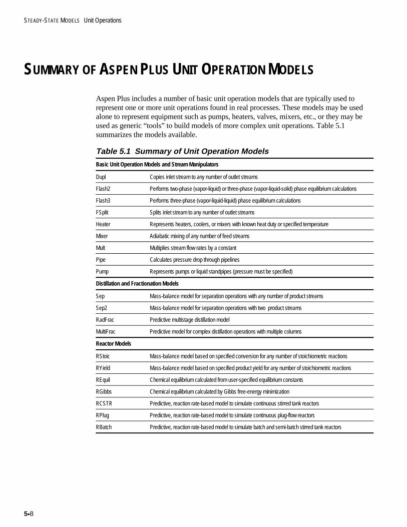
SUMMARY OF ASPEN PLUS UNIT OPERATION MODELS
Aspen Plus includes a number of basic unit operation models that are typically used torepresent one or more unit operations found in real processes. These models may be usedalone to represent equipment such as pumps, heaters, valves, mixers, etc., or they may beused as generic “tools” to build models of more complex unit operations. Table 5.1summarizes the models available.
Table 5.1 Summary of Unit Operation Models
Basic Unit Operation Models and Stream Manipulators
Dupl Copies inlet stream to any number of outlet streams
Flash2 Performs two-phase (vapor-liquid) or three-phase (vapor-liquid-solid) phase equilibrium calculations
Flash3 Performs three-phase (vapor-liquid-liquid) phase equilibrium calculations
FSplit Splits inlet stream to any number of outlet streams
Heater Represents heaters, coolers, or mixers with known heat duty or specified temperature
Mixer Adiabatic mixing of any number of feed streams
Mult Multiplies stream flow rates by a constant
Pipe Calculates pressure drop through pipelines
Pump Represents pumps or liquid standpipes (pressure must be specified)
Distillation and Fractionation Models
Sep Mass-balance model for separation operations with any number of product streams
Sep2 Mass-balance model for separation operations with two product streams
RadFrac Predictive multistage distillation model
MultiFrac Predictive model for complex distillation operations with multiple columns
Reactor Models
RStoic Mass-balance model based on specified conversion for any number of stoichiometric reactions
RYield Mass-balance model based on specified product yield for any number of stoichiometric reactions
REquil Chemical equilibrium calculated from user-specified equilibrium constants
RGibbs Chemical equilibrium calculated by Gibbs free-energy minimization
RCSTR Predictive, reaction rate-based model to simulate continuous stirred tank reactors
RPlug Predictive, reaction rate-based model to simulate continuous plug-flow reactors
RBatch Predictive, reaction rate-based model to simulate batch and semi-batch stirred tank reactors
Polymers Plus User Guide 5x9
Dupl The Dupl block copies one inlet stream to two or more outlet streams. By design, themass flow rate and attribute rates out of this block will be greater than the flow rates intothe block, violating mass and attribute conservation principles.
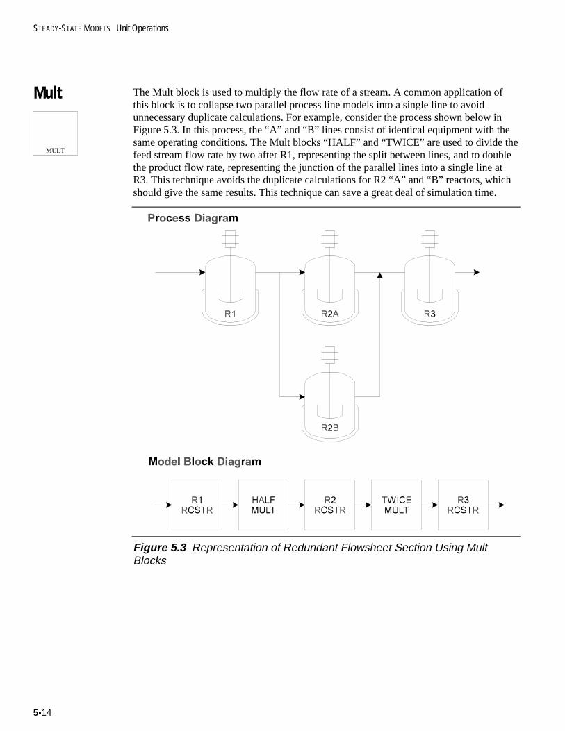
Frequently, the Dupl block is used as a shortcut to reduce the simulation time required tomodel a process consisting of two or more parallel process lines. For example, considerthe process shown in Figure 5.2. The second unit (“R2A” and “R2B”) in the “A” and “B”lines consist of identical unit operations operating at the same conditions. The third unit(“R3A” and “R3B”) operates differently in the two lines. Since the process lines areidentical up to the third unit, there is no need to include both process lines in the model.Instead, we can consider one line, such as “A” and duplicate the outlet stream at the pointwhere the process conditions diverge from each other.
Another application of the Dupl model is to carry out simple case studies. For example,assume there are two proposed scenarios for carrying out a given reaction. In the firstscenario, the reaction is carried out at a high temperature in a small reactor with a shortresidence time. In the second scenario, the reaction is carried out at a low temperature in alarge reactor with high residence times. The two reactors can be placed in a single flowsheet model. The duplicator block is used to copy one feed stream to both reactors. Thetwo “cases” can be compared by examining the stream summary.
STEADY-STATE MODELS Unit Operations
5x10
Operating Conditions
R1A R1B R2A R2B R3A R3B
Temperature, qqC 250 250 260 260 270 265
Pressure, torr 760 760 1200 1200 1500 1700
Volume, liter 2000 2000 1500 1500 1000 1200
Figure 5.2 Using Dupl Block to Eliminate Redundant Calculations
Polymers Plus User Guide 5x11
Flash2 The Flash2 block carries out a phase-equilibrium calculation for a vapor-liquid split. The“chemistry” feature of this block can be used to extend the phase equilibrium to vapor-liquid-solid systems. The free-water option can be used to extend the phase equilibriumcalculations to include a free water phase in addition to the organic liquid phase.
The Flash2 model can be used to simulate simple flash drums with any number of feedstreams. The model is also a good tool for representing spray condensers, single-stagedistillations, knock-back condensers, decanters, and other types of equipment whicheffectively operate as one ideal stage.
The Flash2 model assumes a perfect phase split, but an entrainment factor can bespecified to account for liquid carryover in the vapor stream. The entrainment factor isspecified by the user, it is not calculated by the model. If a correlation between the vaporflow rate and the entrainment rate is available, this correlation can be applied to the modelusing a Fortran block which reads the vapor flow rate calculated by the Flash block,calculates the entrainment rate, and writes the resulting prediction back to the Flash block.Note that this approach creates an information loop in the model which must beconverged.
The Flash2 block does not fractionate the polymer molecular weight distribution. Instead,the molecular weight distribution of the polymer in each product stream is assumed to bethe same as the feed stream.
Flash3 The Flash3 block carries out phase-equilibrium calculations for a vapor-liquid-liquidsplits. The liquid phases may be organic-organic (including polymer-monomer) oraqueous-organic. For aqueous-organic systems, the Flash3 model is more rigorous thanthe Flash2/free water approach described above. The key difference is that the Flash3model considers dissolved organic compounds in the aqueous phase while the free waterapproach assumes a pure water phase.
Generally, three-phase flashes are more difficult to converge than two-phase flashes.Three-phase flash failures may indicate bad binary interaction parameters between thecomponents. The problem may also stem from bogus vapor pressures or heats offormation. In general, it is a good idea to study two-phase splits for the system in questionbefore attempting to model a three-phase decanter or reactor.
STEADY-STATE MODELS Unit Operations
5x12
As with the two-phase flash, the three-phase flash is more stable if temperature andpressure are specified. Other options, such as duty and vapor fraction, are more difficult toconverge. Temperature estimates may aid convergence in duty-specified reactors.
The Flash3 block does not fractionate the polymer molecular weight distribution. Instead,the molecular weight distribution of the polymer in each product stream is assumed to bethe same as the feed stream.
FSplit The flow splitter block, FSplit, is used to represent valves or tanks with several outlets.The outlet flow rates can be specified on a mass, mole, or volume basis, or they can bespecified as a fraction of the feed stream. In general, the fraction specifications are bestbecause they are independent of the feed stream flow rates. This makes the model moreflexible and reliable when using tools like SENSITIVITY or DESIGN-SPEC which mightdirectly or indirectly manipulate the stream which is being split. The FSplit block can alsobe used with reactor models to account for back-mixing.
The FSplit block assumes that the class 2 polymer attributes split according to massmixing rules. For example, if the outlet stream is split 60:40, then the class 2 attributes,such as the segment flow rates, are also split 60:40. This approach is identical to assumingthat the properties of the polymer in each outlet stream are the same as the properties ofthe polymer in the inlet stream.
Heater Heater can be used to represent heaters, coolers, mixers, valves, or tanks. The Heaterblock allows you to specify the temperature or heat duty of the unit, but does not carry outrigorous heat exchange equations. Any number of feed streams can be specified for theHeater block. This block follows the same mixing rules as the Mixer model.
Polymers Plus User Guide 5x13
Mixer The mixer block, Mixer, is used to mix two or more streams to form a single mixed outlet.The mixer block can be used to represent mixing tanks, static mixers, or simply the unionof two pipes in a tee. The Mixer model assumes ideal, adiabatic mixing. The pressure ofthe mixer can be specified as an absolute value or as a drop relative to the lowest feedstream pressure.
The Mixer model is functionally equal to the Heater model, except it only allowsadiabatic mixing. For this reason, the Heater model may be a better choice for modelingmixing tanks.
The Mixer block assumes that the class 2 polymer attributes are additive. For example ifstream “A” and “B” are mixed to form stream “C”, and the zeroth moments of a polymerin stream “A” and “B” are 12 kmol/sec and 15 kmol/sec, then the polymer in the productstream has a zeroth moment of 12+15=27 kmol/sec.
STEADY-STATE MODELS Unit Operations
5x14
Mult The Mult block is used to multiply the flow rate of a stream. A common application ofthis block is to collapse two parallel process line models into a single line to avoidunnecessary duplicate calculations. For example, consider the process shown below inFigure 5.3. In this process, the “A” and “B” lines consist of identical equipment with thesame operating conditions. The Mult blocks “HALF” and “TWICE” are used to divide thefeed stream flow rate by two after R1, representing the split between lines, and to doublethe product flow rate, representing the junction of the parallel lines into a single line atR3. This technique avoids the duplicate calculations for R2 “A” and “B” reactors, whichshould give the same results. This technique can save a great deal of simulation time.
Figure 5.3 Representation of Redundant Flowsheet Section Using MultBlocks
Polymers Plus User Guide 5x15
Pump The Pump block changes the pressure of a stream. This block can be used to represent anactual pump, or it can be used to represent pressure increases due to liquid head instandpipes.
Pipe The Pipe model is used to calculate pressure drops in pipelines. The algorithms in thismodel are not designed for non-ideal fluids such as polymers, so the pipe model should beused with caution in polymer process models. A better option to calculate pressure dropsin polymer pipelines is to use RPlug with a user-written pressure-drop subroutine.
Sep The Sep block is a generic separation model which allows component fractionationbetween two or more product streams. The products can be split according to flow rate orfractional specifications. The Sep block is commonly used to represent distillationcolumns or other separation equipment when the product stream purity is well known andthe details of the separation process are not important.
The Sep block does not fractionate the polymer molecular weight distribution. Instead, themolecular weight distribution of the polymer in each product stream is assumed to be thesame as the feed stream.
Sep2 The Sep2 block is a generic separation model which allows component fractionationbetween two product streams. The products can be split according to flow rate orfractional specifications. The Sep2 block is commonly used to represent distillationcolumns or other separation equipment when the product stream purity is well known andthe details of the separation process are not important. Compared to the Sep block, theSep2 block has more flexible input options, but it only allows two outlet streams.
The Sep2 block does not fractionate the polymer molecular weight distribution. Instead,the molecular weight distribution of the polymer in each product stream is assumed to bethe same as the feed stream.
STEADY-STATE MODELS Unit Operations
5x16
DISTILLATION MODELS
Aspen Plus includes several shortcut distillation models (DISTL, SFRAC, etc.) which canbe used to represent distillation columns. These blocks do not fractionate the polymermolecular weight distribution. Instead, the molecular weight distribution of the polymer ineach product stream is assumed to be the same as the feed stream. The class-2 componentattributes in each product stream are set proportional to the mass flow rate of the attributedcomponent in each product stream.
With the exception of the RadFrac model, the rigorous distillation models in Aspen Plusdo not account for component attributes.
RadFrac The RadFrac block is a rigorous multistage distillation model for two- and three-phasesystems. RadFrac allows polymer feed streams at any tray, but it does not account forpolymerization reaction kinetics. The molecular weight distribution and other polymerproperties are not fractionated between the phases. Instead, the class-2 componentattributes of the polymer components are split at each stage in proportion to the polymercomponent mass fractions. For example, if 90% of the polymer fed to a given tray goes tothe liquid phase leaving that tray, then 90% of the zeroth moment and other class-2attributes are assigned to the liquid phase on that tray.
REACTOR MODELS
Aspen Plus includes three classes of reactor models which include various levels of rigorand predictive capability. These classes are: (1) mass-balance models; (2) equilibriummodels; and (3) rigorous kinetic models.
The least predictive models, RStoic and RYield, calculate output flow rates based onuser-specified input flow rates. If polymer components are involved in the reactions, thenthe component attributes associated with the polymer components must be specified forthe product stream. These models calculate the mass and energy balances, but they do notperform rigorous kinetic calculations.
The RGibbs and REquil models assume chemical and phase equilibrium. When polymercomponents are involved in the reactions, then the specified stoichiometry must beconsistent with the reference molecular weight of the polymer component. In addition, thecomponent attribute values for the polymer product must be specified by the user. Sincethe solution algorithms for these models do not consider the influence of the segmentalcomposition of polymer components, they cannot be applied to copolymers.
Polymers Plus User Guide 5x17
Rigorous kinetic models include RCSTR (continuous stirred tank reactor), RPlug (plug-flow reactor model), and RBatch (batch stirred tank reactor). Each of these models canconsider one, two, or three reacting phases. These reactor models are with the reactionkinetic models to predict product stream composition and flow rates based on calculatedreaction rates.
MASS-BALANCE REACTOR MODELS
RStoic The RStoic reactor model is used to represent reaction equipment when reaction kineticsare unknown or are unimportant, for example when reactions are very fast and proceeduntil the limiting reagent is exhausted. RStoic requires knowledge of the net reactionstoichiometry, and the extent of reaction or conversion of a key component.
RStoic calculates the product stream flow rates based on user-specified reactionstoichiometries and extent of reaction or conversion of a key component. The reactionstoichiometry statements may include monomers, oligomers, or polymers, but may notinclude segments. Instead, the segment information (SFLOW or SFRAC) must bespecified as component attributes in the COMP-ATTR sentence.
If polymer components are involved in any of the reactions, use the COMP-ATTR form tospecify molecular weight values (MWN, MWW or PDI) or degree of polymerization(DPN, DPW or PDI ) for the polymer products. Specify the SFRAC attribute forhomopolymers or copolymers with a known product polymer composition. Forcopolymers with product compositions which depend on the feed flow rates of monomersor polymer segments, specify dummy values for the SFLOW attribute and use a user-written Fortran block to predict product segment flow rates which are consistent with thecalculated product flow rates. Write the calculated results into the product stream of theRStoic block.
When some of the specified reactions involve polymers, the reaction stoichiometry mustbe written in a manner consistent with the reference molecular weight of the polymercomponent. Otherwise, the mass and energy balance calculations will not be consistent.
STEADY-STATE MODELS Unit Operations
5x18
RYield The RYield reactor model is used to represent reaction equipment when reaction kineticsare unknown or are unimportant, and the reactions result in a product distribution with aknown yield.
RYield calculates the product stream flow rates based on user-specified reactionstoichiometries and yield distributions. The reaction stoichiometry statements mayinclude monomers, oligomers, or polymers, but may not include segments. Instead, thesegment information (SFLOW or SFRAC) must be specified as component attributes inthe COMP-ATTR sentence.
If polymer components are involved in any of the reactions, use the COMP-ATTR form tospecify molecular weight values (MWN, MWW or PDI) or degree of polymerization(DPN, DPW or PDI ) for the polymer products. Specify the SFRAC attribute forhomopolymers or copolymers with a known product polymer composition. Forcopolymers with product compositions which depend on the feed flow rates of monomersor polymer segments, specify dummy values for the SFLOW attribute and use a user-written Fortran block to predict product segment flow rates which are consistent with thecalculated yield. Write the calculated results into the product stream of the RYield block.
When some of the specified reactions involve polymers, the reaction stoichiometry mustbe written in a manner consistent with the reference molecular weight of the polymercomponent. Otherwise, the mass and energy balance calculations will not be consistent.
Polymers Plus User Guide 5x19
EQUILIBRIUM REACTOR MODELS
REquil The REquil model calculates product stream flow rates using equilibrium constantsdetermined from Gibbs free energy. The equilibrium constants are based on user-specifiedreaction stoichiometries and yield distributions. The reaction stoichiometry statementsmay include monomers or oligomers, but may not include polymers or segments. If thefeed stream includes polymer components, the attributes of the polymer components willbe copied to the outlet stream.
RGibbs The RGibbs model uses the Gibbs free energy minimization technique to determine thecomposition of each phase. This algorithm cannot predict the product of equilibriumpolymerization reactions. Polymer phase equilibrium, however, can be predicted by themodel. The RGibbs phase equilibrium algorithm assumes that the composition andmolecular weight distribution of a polymer component is equal in each of the productphases. The class-2 component attributes of the polymer component are set in proportionto the mass flow of the polymer component in each of the product phases. The mass flowrates in the product phases are set by the Gibbs free energy minimization algorithm.
To properly split component attributes among the RGibbs solution phases, use the "Phaseequilibrium only" option. With this the model can predict multiple liquid phases such asthree liquid phases. Surface tension effects are not considered. If you are certain that therewill be no vapor phase, uncheck the "Include vapor phase" box to speed up calculations.Use one outlet stream for each predicted phase, to separate out the component attributesof that phase.
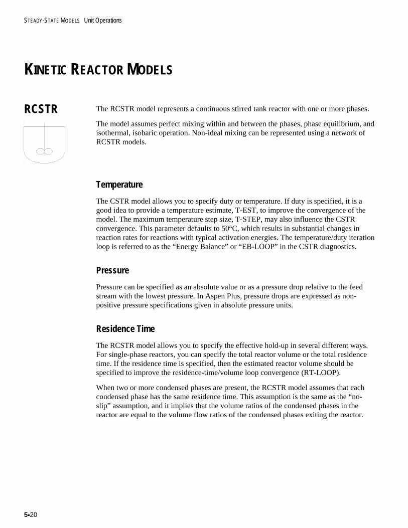
STEADY-STATE MODELS Unit Operations
5x20
KINETIC REACTOR MODELS
RCSTR The RCSTR model represents a continuous stirred tank reactor with one or more phases.
The model assumes perfect mixing within and between the phases, phase equilibrium, andisothermal, isobaric operation. Non-ideal mixing can be represented using a network ofRCSTR models.
Temperature
The CSTR model allows you to specify duty or temperature. If duty is specified, it is agood idea to provide a temperature estimate, T-EST, to improve the convergence of themodel. The maximum temperature step size, T-STEP, may also influence the CSTRconvergence. This parameter defaults to 50qC, which results in substantial changes inreaction rates for reactions with typical activation energies. The temperature/duty iterationloop is referred to as the “Energy Balance” or “EB-LOOP” in the CSTR diagnostics.
Pressure
Pressure can be specified as an absolute value or as a pressure drop relative to the feedstream with the lowest pressure. In Aspen Plus, pressure drops are expressed as non-positive pressure specifications given in absolute pressure units.
Residence Time
The RCSTR model allows you to specify the effective hold-up in several different ways.For single-phase reactors, you can specify the total reactor volume or the total residencetime. If the residence time is specified, then the estimated reactor volume should bespecified to improve the residence-time/volume loop convergence (RT-LOOP).
When two or more condensed phases are present, the RCSTR model assumes that eachcondensed phase has the same residence time. This assumption is the same as the “no-slip” assumption, and it implies that the volume ratios of the condensed phases in thereactor are equal to the volume flow ratios of the condensed phases exiting the reactor.
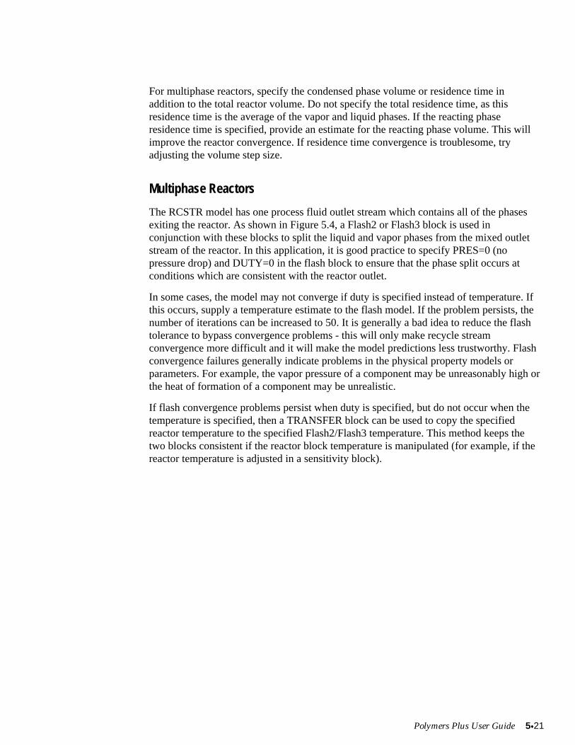
Polymers Plus User Guide 5x21
For multiphase reactors, specify the condensed phase volume or residence time inaddition to the total reactor volume. Do not specify the total residence time, as thisresidence time is the average of the vapor and liquid phases. If the reacting phaseresidence time is specified, provide an estimate for the reacting phase volume. This willimprove the reactor convergence. If residence time convergence is troublesome, tryadjusting the volume step size.
Multiphase Reactors
The RCSTR model has one process fluid outlet stream which contains all of the phasesexiting the reactor. As shown in Figure 5.4, a Flash2 or Flash3 block is used inconjunction with these blocks to split the liquid and vapor phases from the mixed outletstream of the reactor. In this application, it is good practice to specify PRES=0 (nopressure drop) and DUTY=0 in the flash block to ensure that the phase split occurs atconditions which are consistent with the reactor outlet.
In some cases, the model may not converge if duty is specified instead of temperature. Ifthis occurs, supply a temperature estimate to the flash model. If the problem persists, thenumber of iterations can be increased to 50. It is generally a bad idea to reduce the flashtolerance to bypass convergence problems - this will only make recycle streamconvergence more difficult and it will make the model predictions less trustworthy. Flashconvergence failures generally indicate problems in the physical property models orparameters. For example, the vapor pressure of a component may be unreasonably high orthe heat of formation of a component may be unrealistic.
If flash convergence problems persist when duty is specified, but do not occur when thetemperature is specified, then a TRANSFER block can be used to copy the specifiedreactor temperature to the specified Flash2/Flash3 temperature. This method keeps thetwo blocks consistent if the reactor block temperature is manipulated (for example, if thereactor temperature is adjusted in a sensitivity block).
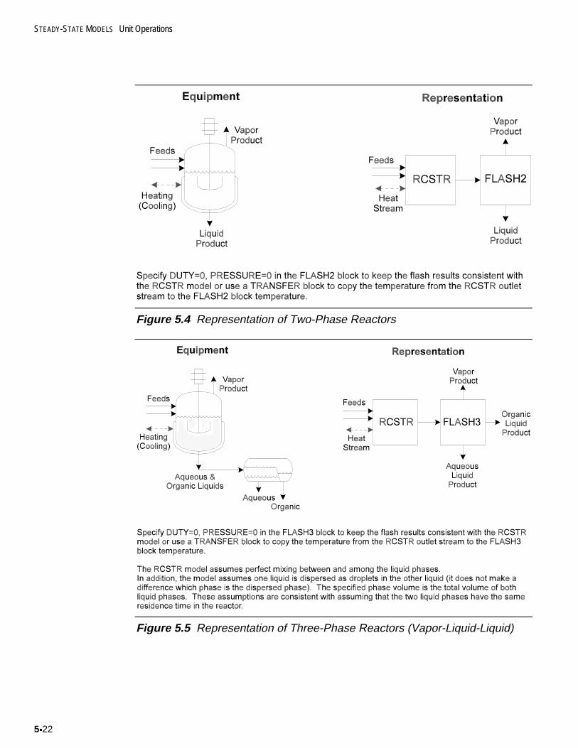
STEADY-STATE MODELS Unit Operations
5x22
Figure 5.4 Representation of Two-Phase Reactors
Figure 5.5 Representation of Three-Phase Reactors (Vapor-Liquid-Liquid)
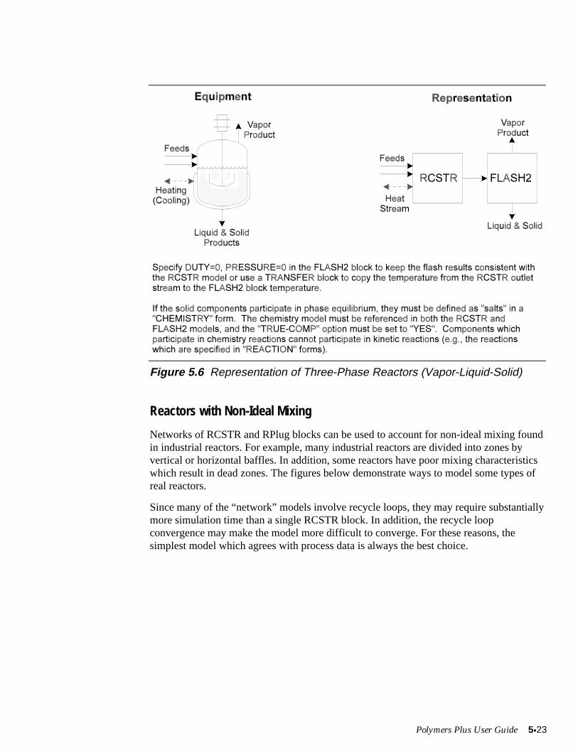
Polymers Plus User Guide 5x23
Figure 5.6 Representation of Three-Phase Reactors (Vapor-Liquid-Solid)
Reactors with Non-Ideal Mixing
Networks of RCSTR and RPlug blocks can be used to account for non-ideal mixing foundin industrial reactors. For example, many industrial reactors are divided into zones byvertical or horizontal baffles. In addition, some reactors have poor mixing characteristicswhich result in dead zones. The figures below demonstrate ways to model some types ofreal reactors.
Since many of the “network” models involve recycle loops, they may require substantiallymore simulation time than a single RCSTR block. In addition, the recycle loopconvergence may make the model more difficult to converge. For these reasons, thesimplest model which agrees with process data is always the best choice.
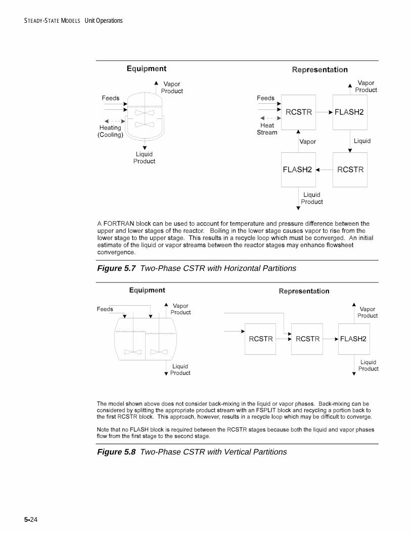
STEADY-STATE MODELS Unit Operations
5x24
Figure 5.7 Two-Phase CSTR with Horizontal Partitions
Figure 5.8 Two-Phase CSTR with Vertical Partitions
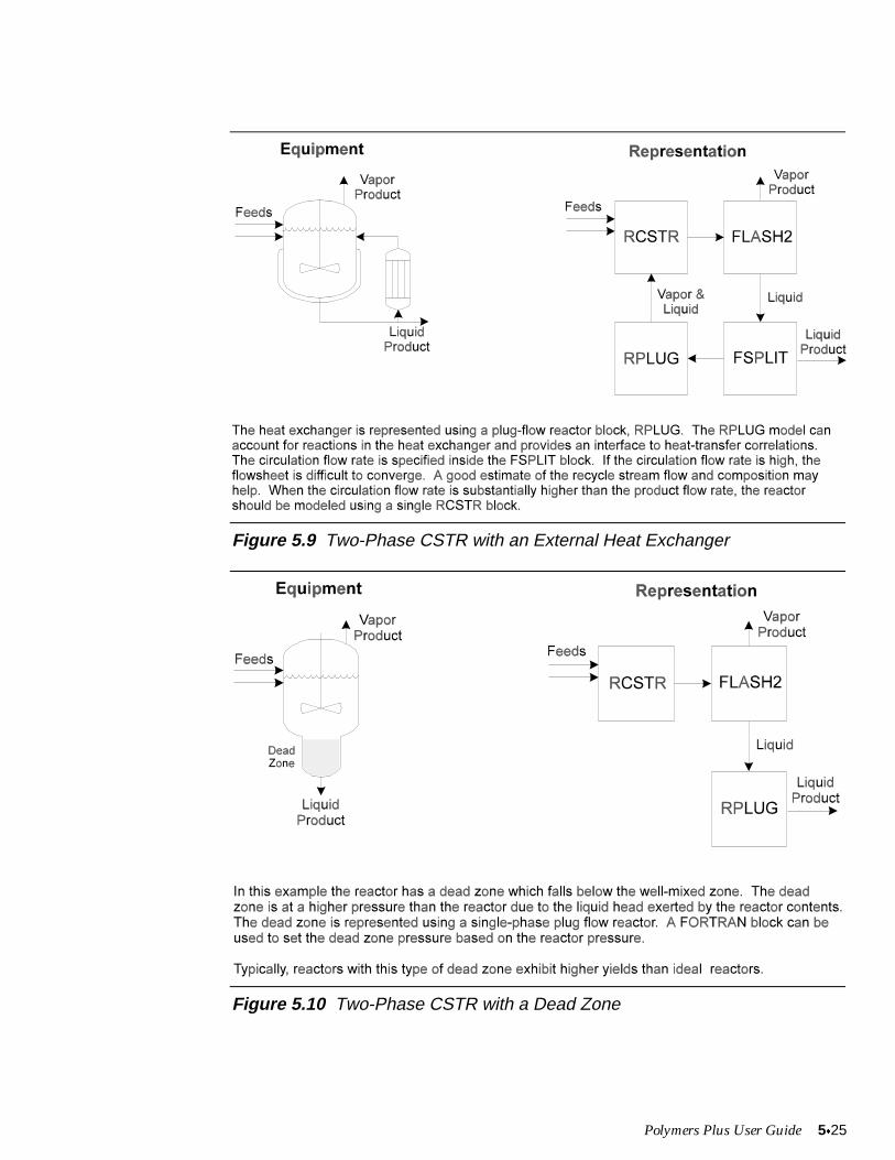
Polymers Plus User Guide 5x25
Figure 5.9 Two-Phase CSTR with an External Heat Exchanger
Figure 5.10 Two-Phase CSTR with a Dead Zone
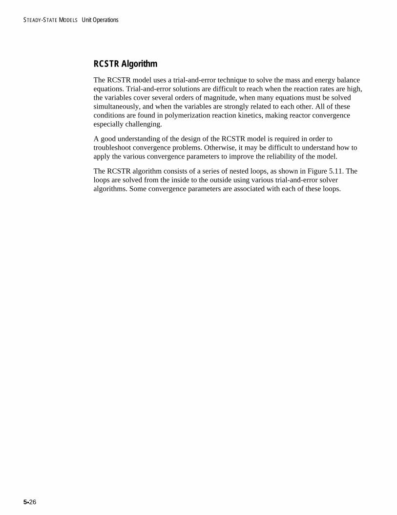
STEADY-STATE MODELS Unit Operations
5x26
RCSTR Algorithm
The RCSTR model uses a trial-and-error technique to solve the mass and energy balanceequations. Trial-and-error solutions are difficult to reach when the reaction rates are high,the variables cover several orders of magnitude, when many equations must be solvedsimultaneously, and when the variables are strongly related to each other. All of theseconditions are found in polymerization reaction kinetics, making reactor convergenceespecially challenging.
A good understanding of the design of the RCSTR model is required in order totroubleshoot convergence problems. Otherwise, it may be difficult to understand how toapply the various convergence parameters to improve the reliability of the model.
The RCSTR algorithm consists of a series of nested loops, as shown in Figure 5.11. Theloops are solved from the inside to the outside using various trial-and-error solveralgorithms. Some convergence parameters are associated with each of these loops.
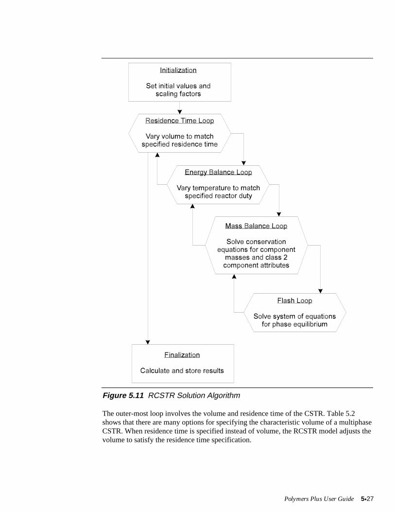
Polymers Plus User Guide 5x27
Figure 5.11 RCSTR Solution Algorithm
The outer-most loop involves the volume and residence time of the CSTR. Table 5.2shows that there are many options for specifying the characteristic volume of a multiphaseCSTR. When residence time is specified instead of volume, the RCSTR model adjusts thevolume to satisfy the residence time specification.
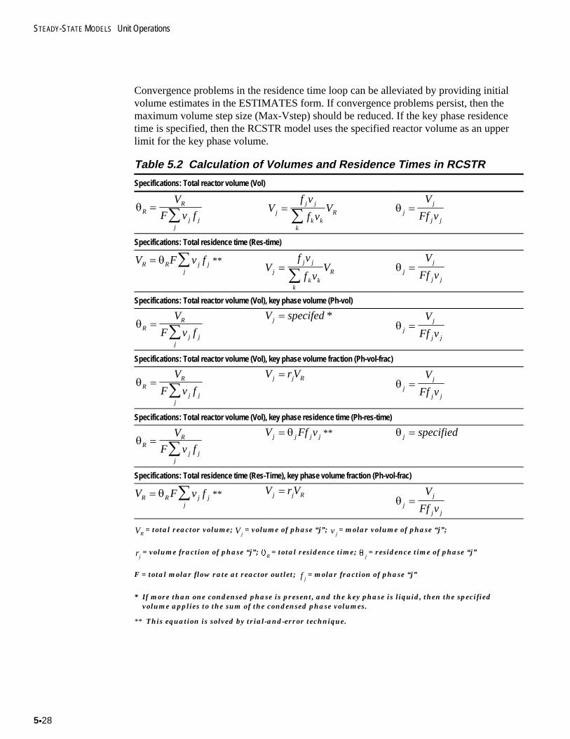
STEADY-STATE MODELS Unit Operations
5x28
Convergence problems in the residence time loop can be alleviated by providing initialvolume estimates in the ESTIMATES form. If convergence problems persist, then themaximum volume step size (Max-Vstep) should be reduced. If the key phase residencetime is specified, then the RCSTR model uses the specified reactor volume as an upperlimit for the key phase volume.
Table 5.2 Calculation of Volumes and Residence Times in RCSTR
Specifications: Total reactor volume (Vol)
TRR
j jj
V
F v f ¦
Vf v
f vVj
j j
k kk
R ¦
T j
j
j j
V
Ff v
Specifications: Total residence time (Res-time)
V F v fR R j jj
¦T **V
f v
f vVj
j j
k kk
R ¦
T j
j
j j
V
Ff v
Specifications: Total reactor volume (Vol), key phase volume (Ph-vol)
TRR
j jj
V
F v f
¦V specifedj *
T j
j
j j
V
Ff v
Specifications: Total reactor volume (Vol), key phase volume fraction (Ph-vol-frac)
TRR
j jj
V
F v f
¦V r Vj j R
T j
j
j j
V
Ff v
Specifications: Total reactor volume (Vol), key phase residence time (Ph-res-time)
TRR
j jj
V
F v f ¦
V Ff vj j j j T ** T j specified
Specifications: Total residence time (Res-Time), key phase volume fraction (Ph-vol-frac)
V F v fR R j jj
¦T ** V r Vj j R T j
j
j j
V
Ff v
VR= total reactor volume; Vj
= volume of phase “j”; vj= molar volume of phase “j”;
r j= volume fraction of phase “j”; TR
= total residence time; T j= residence time of phase “j”
F = total molar flow rate at reactor outlet; f j= molar fraction of phase “j”
* If more than one condensed phase is present, and the key phase is liquid, then the specifiedvolume applies to the sum of the condensed phase volumes.
** This equation is solved by trial-and-error technique.
Polymers Plus User Guide 5x29
EB LOOP The second loop is the energy balance conservation equation (EB-LOOP). In this loop,the reactor temperature is adjusted to match the specified reactor duty. If the temperatureis specified instead of the duty, this loop is by-passed.
Since the reaction rates are very sensitive to temperature, large changes in the reactortemperature between energy-balance iterations (EB-ITER) may cause the mass-balanceloop (MB-LOOP) to diverge. This problem can be solved by providing a goodtemperature estimate (T-EST) in the ESTIMATES form. If the problem persists, themaximum temperature step size (Max-Tstep) should be reduced (the default, 50qC, israther large).
MB-LOOP The next loop is the mass-balance loop (MB-LOOP). This loop uses a multivariablesolver to converge the conservation equations for component mole flow and for the classtwo component attributes.
Two solvers are available: Broyden and Newton. The Broyden algorithm tends to berelatively fast, but it may be unstable if the number of components and attributes is largeand the reaction rates are high. The Newton algorithm tends to be slower, but more stablefor many classes of problems. The Newton algorithm calculates the response of eachvariable to each other variable by perturbing the variables one at a time by a very smallamount. These perturbation steps require lots of simulation time, which makes eachiteration of the Newton algorithm slow.
The number of mass-balance iterations (MB-Maxit) is defined on the convergence form.By default, the model allows 50 mass-balance iterations. This default is sufficient for theNewton algorithm, but is usually too small for the Broyden algorithm. For polymerreaction kinetics, the number of required mass-balance iterations may be as high as 500.
Using a DampingFactor
The stability of the Broyden algorithm can be adjusted using a damping factor (DAMP-FAC) defined on the “Convergence” form. Decreasing the damping factor decreases thestep-size, resulting in a larger number of smaller, more stable steps. Thus, the maximumnumber of iterations should be increased as the damping factor is decreased.
The damping factor is sensitive on a log scale. If the Broyden algorithm appears unstable,try setting the damping factor to 0.5, 0.3, 0.1, 0.05 etc. Optimum damping factors forpolymerization kinetics typically fall between 0.1 and 0.001.
The conservation equations have the form:
accumulation input output Generation � �
For the component mole balance equations: R
S
F
S
F
S
G V
Si
i
iin
i
iout
i
i j jj
i
� �¦ ,
For the class-2 component attributes equations: R
S
A
S
A
S
G V
Si
i
iin
i
iout
i
i j jj
i
� �¦ ' ,
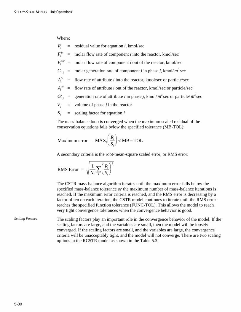
STEADY-STATE MODELS Unit Operations
5x30
Where:
Ri = residual value for equation i, kmol/sec
Fiin = molar flow rate of component i into the reactor, kmol/sec
Fiout = molar flow rate of component i out of the reactor, kmol/sec
Gi j, = molar generation rate of component i in phase j, kmol/m3 sec
Aiin = flow rate of attribute i into the reactor, kmol/sec or particle/sec
Aiout = flow rate of attribute i out of the reactor, kmol/sec or particle/sec
cGi j, = generation rate of attribute i in phase j, kmol/m3 sec or particle/m3 sec
Vj = volume of phase j in the reactor
Si = scaling factor for equation i
The mass-balance loop is converged when the maximum scaled residual of theconservation equations falls below the specified tolerance (MB-TOL):
Maximum error = MAX MB TOLi
R
Si
i
§
©¨
·
¹¸ � �
A secondary criteria is the root-mean-square scaled error, or RMS error:
RMS Error = 1
2
N
R
Si
i
ii
§
©¨
·
¹¸¦
The CSTR mass-balance algorithm iterates until the maximum error falls below thespecified mass-balance tolerance or the maximum number of mass-balance iterations isreached. If the maximum error criteria is reached, and the RMS error is decreasing by afactor of ten on each iteration, the CSTR model continues to iterate until the RMS errorreaches the specified function tolerance (FUNC-TOL). This allows the model to reachvery tight convergence tolerances when the convergence behavior is good.
Scaling Factors The scaling factors play an important role in the convergence behavior of the model. If thescaling factors are large, and the variables are small, then the model will be looselyconverged. If the scaling factors are small, and the variables are large, the convergencecriteria will be unacceptably tight, and the model will not converge. There are two scalingoptions in the RCSTR model as shown in the Table 5.3.
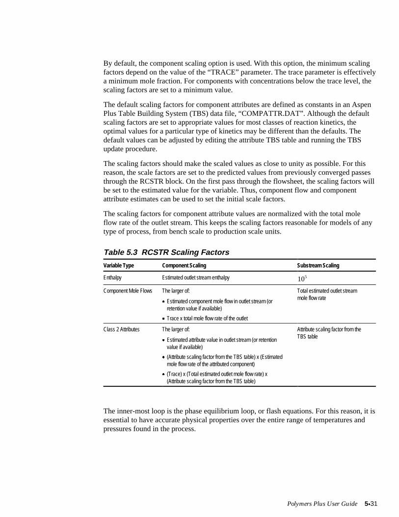
Polymers Plus User Guide 5x31
By default, the component scaling option is used. With this option, the minimum scalingfactors depend on the value of the “TRACE” parameter. The trace parameter is effectivelya minimum mole fraction. For components with concentrations below the trace level, thescaling factors are set to a minimum value.
The default scaling factors for component attributes are defined as constants in an AspenPlus Table Building System (TBS) data file, “COMPATTR.DAT”. Although the defaultscaling factors are set to appropriate values for most classes of reaction kinetics, theoptimal values for a particular type of kinetics may be different than the defaults. Thedefault values can be adjusted by editing the attribute TBS table and running the TBSupdate procedure.
The scaling factors should make the scaled values as close to unity as possible. For thisreason, the scale factors are set to the predicted values from previously converged passesthrough the RCSTR block. On the first pass through the flowsheet, the scaling factors willbe set to the estimated value for the variable. Thus, component flow and componentattribute estimates can be used to set the initial scale factors.
The scaling factors for component attribute values are normalized with the total moleflow rate of the outlet stream. This keeps the scaling factors reasonable for models of anytype of process, from bench scale to production scale units.
Table 5.3 RCSTR Scaling Factors
Variable Type Component Scaling Substream Scaling
Enthalpy Estimated outlet stream enthalpy 105
Component Mole Flows The larger of:
x Estimated component mole flow in outlet stream (orretention value if available)
x Trace x total mole flow rate of the outlet
Total estimated outlet streammole flow rate
Class 2 Attributes The larger of:
x Estimated attribute value in outlet stream (or retentionvalue if available)
x (Attribute scaling factor from the TBS table) x (Estimatedmole flow rate of the attributed component)
x (Trace) x (Total estimated outlet mole flow rate) x(Attribute scaling factor from the TBS table)
Attribute scaling factor from theTBS table
The inner-most loop is the phase equilibrium loop, or flash equations. For this reason, it isessential to have accurate physical properties over the entire range of temperatures andpressures found in the process.
STEADY-STATE MODELS Unit Operations
5x32
The flash calculations start from retention values once the mass-balance error falls belowthe retention threshold (Ret-Thresh) specified in the convergence form. If the retentionthreshold is set very high, then the flash may fail, resulting in step-size cuts in the massbalance loop. If the retention threshold is reduced, the reactor calculations may requiremore time. For most simulation problems, setting the retention threshold to 1 1010uresults in fast flash convergence without errors. If errors occur, try using the default value,1 105u . If errors persist, the most likely cause is a physical property problem.
Integration Initialization
The convergence behavior of the RCSTR model depends on how the model is initialized.There are two initialization options for the RCSTR model. By default, the RCSTR modelinitialized the solver as described below. Optionally, the RCSTR model can be initializedusing an integration approach.
In the integration algorithm, the RCSTR is treated as a dynamic stirred-tank reactor. Theconservation equations are numerically integrated from an initial condition to the steady-state condition. The initial compositions in the reactor are set equal to those in the feedstream.
If temperature is specified in the reactor, then the temperature profile during initializationcan be ramped from the feed stream temperature to the specified temperature over theinterval of several residence times. If duty is specified, then the duty can be ramped fromadiabatic conditions to the specified duty. Ramping allows the reactor to “cold-start” forimproved integration performance.
The numerical integration carries forward until the residual terms (accumulation terms)drop below the specified mass-balance tolerance. At this point, the model enters thesolver and continues until the model converges.
Note that initial guesses for component flow rates and component attributes should not beprovided when using the integration initialization option.
Solver Initialization
By default, the solver algorithm initializes itself based on previously-saved results(retention). This saves time if the RCSTR block is inside a flowsheet recycle loop, wherethe block will be run several times in succession. This also saves time if the block isinside a sensitivity, optimization, design-spec, or data-fit study. The retention values areignored if the “RESTART” switch in the “Block-Options” form is set to “YES”.
If the “RESTART” flag is “YES”, or during the first pass through the model, the modelwill initialize according to user-specified estimates. Estimates can be provided for thereactor volume, phase volume, reactor temperature, component flow rates, and componentattribute values. The component attribute estimates can be specified using class-2 orclass-0 attribute values.
Polymers Plus User Guide 5x33
If estimates are not provided, then the model assumes that the outlet stream conditionsequal the inlet stream conditions.
Troubleshooting Convergence Problems
To diagnose RCSTR convergence problems, set the terminal reporting level to “7” in theBlock-Options form. This causes the RCSTR model to report the residence time iterations(RT-ITER), energy balance iterations (EB-ITER), and mass-balance iterations (MB-ITER) to the control panel. In addition, the model reports the maximum and root-mean-square errors for each loop.
The history level controls the diagnostic messages written to the history file (.HIS file).The maximum mass-balance error is reported at level 5. At level 6, the model reports thevalue of each reacting component flow rate and each component attribute. At level 7, themodel reports values and rates of change (reaction rates) for components and attributes.
First, simplify the problem by specifying temperature and volume instead of duty andresidence time. If convergence problems persist, they must be related to the mass-balanceloop, the reaction kinetic model or rate constants, or the underlying physical propertycalculations.
Numerical integration is much more reliable than trial-and-error solvers. If the RCSTRmass-balance fails to converge, try running the same kinetics in an RPlug model. Ifpossible, set the phase criteria “liquid-only” to eliminate physical property problems fromthe list of possible sources of error. If the RPlug model cannot converge with the specifiedkinetics, then the problem is almost certainly related to reaction kinetics.
Possible sources of error in the reaction kinetics include:
x Errors in the molecular weight of a product or reactantx Errors in the specified stoichiometry of a reaction (mass balance is violated)x Unreasonable rate constants, especially activation energies (verify the units)x Reactions with zeroth-order reactants which are not presentx Unreasonable concentrations of catalysts or inhibitors (put the feed stream in a flash
block and verify that the concentrations in the reacting phase make sense).x Errors in user-written Fortran subroutines.
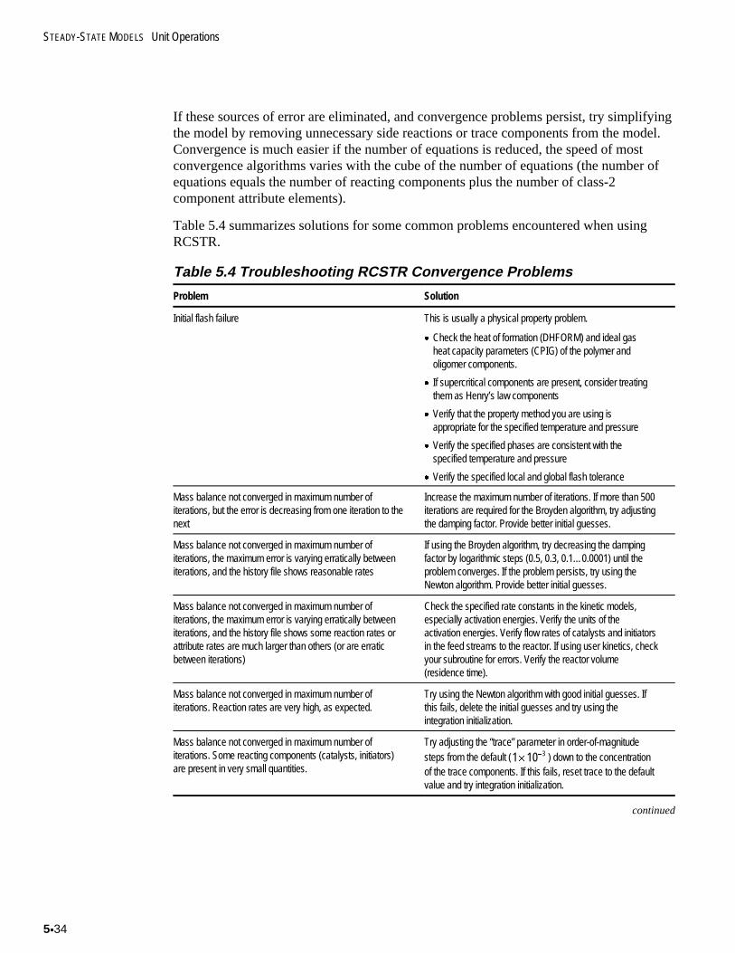
STEADY-STATE MODELS Unit Operations
5x34
If these sources of error are eliminated, and convergence problems persist, try simplifyingthe model by removing unnecessary side reactions or trace components from the model.Convergence is much easier if the number of equations is reduced, the speed of mostconvergence algorithms varies with the cube of the number of equations (the number ofequations equals the number of reacting components plus the number of class-2component attribute elements).
Table 5.4 summarizes solutions for some common problems encountered when usingRCSTR.
Table 5.4 Troubleshooting RCSTR Convergence Problems
Problem Solution
Initial flash failure This is usually a physical property problem.
x Check the heat of formation (DHFORM) and ideal gasheat capacity parameters (CPIG) of the polymer andoligomer components.
x If supercritical components are present, consider treatingthem as Henry’s law components
x Verify that the property method you are using isappropriate for the specified temperature and pressure
x Verify the specified phases are consistent with thespecified temperature and pressure
x Verify the specified local and global flash tolerance
Mass balance not converged in maximum number ofiterations, but the error is decreasing from one iteration to thenext
Increase the maximum number of iterations. If more than 500iterations are required for the Broyden algorithm, try adjustingthe damping factor. Provide better initial guesses.
Mass balance not converged in maximum number ofiterations, the maximum error is varying erratically betweeniterations, and the history file shows reasonable rates
If using the Broyden algorithm, try decreasing the dampingfactor by logarithmic steps (0.5, 0.3, 0.1…0.0001) until theproblem converges. If the problem persists, try using theNewton algorithm. Provide better initial guesses.
Mass balance not converged in maximum number ofiterations, the maximum error is varying erratically betweeniterations, and the history file shows some reaction rates orattribute rates are much larger than others (or are erraticbetween iterations)
Check the specified rate constants in the kinetic models,especially activation energies. Verify the units of theactivation energies. Verify flow rates of catalysts and initiatorsin the feed streams to the reactor. If using user kinetics, checkyour subroutine for errors. Verify the reactor volume(residence time).
Mass balance not converged in maximum number ofiterations. Reaction rates are very high, as expected.
Try using the Newton algorithm with good initial guesses. Ifthis fails, delete the initial guesses and try using theintegration initialization.
Mass balance not converged in maximum number ofiterations. Some reacting components (catalysts, initiators)are present in very small quantities.
Try adjusting the “trace” parameter in order-of-magnitudesteps from the default (1 10 3
u� ) down to the concentration
of the trace components. If this fails, reset trace to the defaultvalue and try integration initialization.
continued
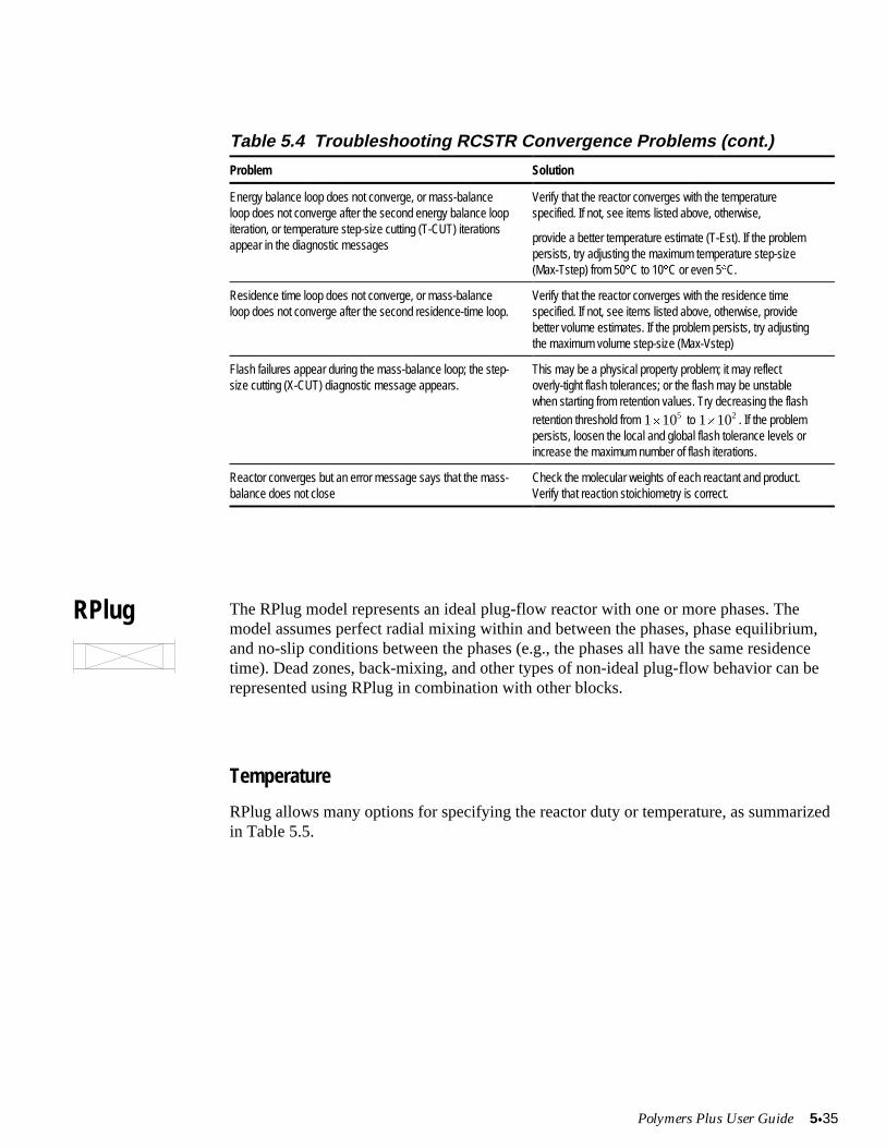
Polymers Plus User Guide 5x35
Table 5.4 Troubleshooting RCSTR Convergence Problems (cont.)
Problem Solution
Energy balance loop does not converge, or mass-balanceloop does not converge after the second energy balance loopiteration, or temperature step-size cutting (T-CUT) iterationsappear in the diagnostic messages
Verify that the reactor converges with the temperaturespecified. If not, see items listed above, otherwise,
provide a better temperature estimate (T-Est). If the problempersists, try adjusting the maximum temperature step-size(Max-Tstep) from 50qC to 10qC or even 5qC.
Residence time loop does not converge, or mass-balanceloop does not converge after the second residence-time loop.
Verify that the reactor converges with the residence timespecified. If not, see items listed above, otherwise, providebetter volume estimates. If the problem persists, try adjustingthe maximum volume step-size (Max-Vstep)
Flash failures appear during the mass-balance loop; the step-size cutting (X-CUT) diagnostic message appears.
This may be a physical property problem; it may reflectoverly-tight flash tolerances; or the flash may be unstablewhen starting from retention values. Try decreasing the flashretention threshold from 1 10u
5 to 1 10u2 . If the problem
persists, loosen the local and global flash tolerance levels orincrease the maximum number of flash iterations.
Reactor converges but an error message says that the mass-balance does not close
Check the molecular weights of each reactant and product.Verify that reaction stoichiometry is correct.
RPlug The RPlug model represents an ideal plug-flow reactor with one or more phases. Themodel assumes perfect radial mixing within and between the phases, phase equilibrium,and no-slip conditions between the phases (e.g., the phases all have the same residencetime). Dead zones, back-mixing, and other types of non-ideal plug-flow behavior can berepresented using RPlug in combination with other blocks.
Temperature
RPlug allows many options for specifying the reactor duty or temperature, as summarizedin Table 5.5.
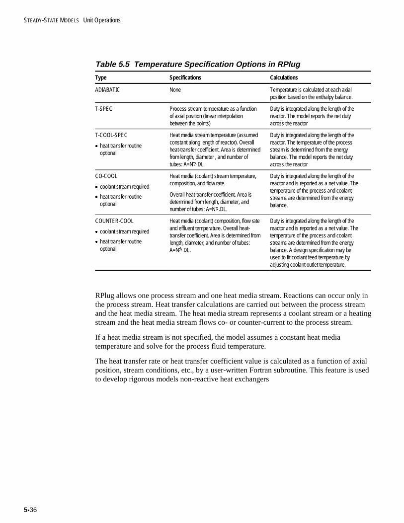
STEADY-STATE MODELS Unit Operations
5x36
Table 5.5 Temperature Specification Options in RPlug
Type Specifications Calculations
ADIABATIC None Temperature is calculated at each axialposition based on the enthalpy balance.
T-SPEC Process stream temperature as a functionof axial position (linear interpolationbetween the points)
Duty is integrated along the length of thereactor. The model reports the net dutyacross the reactor
T-COOL-SPEC
x heat transfer routineoptional
Heat media stream temperature (assumedconstant along length of reactor). Overallheat-transfer coefficient. Area is determinedfrom length, diameter , and number oftubes: A=N%DL
Duty is integrated along the length of thereactor. The temperature of the processstream is determined from the energybalance. The model reports the net dutyacross the reactor
CO-COOL
x coolant stream required
x heat transfer routineoptional
Heat media (coolant) stream temperature,composition, and flow rate.
Overall heat-transfer coefficient. Area isdetermined from length, diameter, andnumber of tubes: A=N%DL.
Duty is integrated along the length of thereactor and is reported as a net value. Thetemperature of the process and coolantstreams are determined from the energybalance.
COUNTER-COOL
x coolant stream required
x heat transfer routineoptional
Heat media (coolant) composition, flow rateand effluent temperature. Overall heat-transfer coefficient. Area is determined fromlength, diameter, and number of tubes:A=N%DL.
Duty is integrated along the length of thereactor and is reported as a net value. Thetemperature of the process and coolantstreams are determined from the energybalance. A design specification may beused to fit coolant feed temperature byadjusting coolant outlet temperature.
RPlug allows one process stream and one heat media stream. Reactions can occur only inthe process stream. Heat transfer calculations are carried out between the process streamand the heat media stream. The heat media stream represents a coolant stream or a heatingstream and the heat media stream flows co- or counter-current to the process stream.
If a heat media stream is not specified, the model assumes a constant heat mediatemperature and solve for the process fluid temperature.
The heat transfer rate or heat transfer coefficient value is calculated as a function of axialposition, stream conditions, etc., by a user-written Fortran subroutine. This feature is usedto develop rigorous models non-reactive heat exchangers
Polymers Plus User Guide 5x37
Pressure
The pressure at the reactor entry can be specified as an absolute value or as a pressuredrop relative to the feed stream. In Aspen Plus, pressure drops are expressed as non-positive pressure specifications given in absolute pressure units.
The pressure drop across the reactor can be specified as a constant or calculated in a user-written Fortran subroutine. If the pressure drop is specified, the model assumes it is linearalong the length of the reactor.
Residence Time
The RPlug model assumes a cylindrical geometry. The length, diameter, and number oftubes are specified. The process fluid is assumed to move through the tubes, and thecoolant is assumed to flow on the outside of the tubes.
The total reactor volume cannot be specified, but the aspect ratio (length/diameter) has noinfluence on the model predictions. Thus, the diameter can be set to 1.12838 units, whichcorresponds to an area of 1.0000 units2 . With this area, the length in units and volume inunits3 have the same numerical value, thus the specified length is equal to the volume.
The phase volumes cannot be specified independently. Instead, the RPlug model assumesthat the phases move through the reactor without slipping past each other. Thisassumption is valid for situations where one phase is dispersed as droplets or bubbles in asecond, continuous phase, such as dew in a vapor phase or small gas bubbles in a liquidphase. This assumption is not valid for multiphase plug flow reactors with controlledlevels.
With this assumption in place, the reactor residence time is equal to the residence time ofeach phase present in the reactor. The residence time is calculated by numericalintegration.
One work-around for the no-slip assumption is to write a user kinetic subroutine (or astep-growth mass-transfer routine) which calls the flash model directly. Then, specify thereactor as liquid-only and set the diameter to the hydraulic diameter of the reactor.
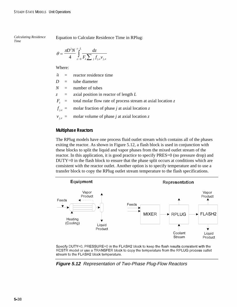
STEADY-STATE MODELS Unit Operations
5x38
Calculating ResidenceTime
Equation to Calculate Residence Time in RPlug:
TS
¦³
D N dz
F f vz j j z j zz
z L2
04 , ,
Where:
� = reactor residence time
D = tube diameter
N = number of tubes
z = axial position in reactor of length L
Fz = total molar flow rate of process stream at axial location z
f j z, = molar fraction of phase j at axial location z
vj z, = molar volume of phase j at axial location z
Multiphase Reactors
The RPlug models have one process fluid outlet stream which contains all of the phasesexiting the reactor. As shown in Figure 5.12, a flash block is used in conjunction withthese blocks to split the liquid and vapor phases from the mixed outlet stream of thereactor. In this application, it is good practice to specify PRES=0 (no pressure drop) andDUTY=0 in the flash block to ensure that the phase split occurs at conditions which areconsistent with the reactor outlet. Another option is to specify temperature and to use atransfer block to copy the RPlug outlet stream temperature to the flash specifications.
Figure 5.12 Representation of Two-Phase Plug-Flow Reactors
Polymers Plus User Guide 5x39
Reactors with Non-Ideal Mixing
Back-mixed plug flow reactors can be modeled using a recycle stream or by breaking thereactor down into a series of RCSTR blocks. The recycle-stream approach has theadvantage of RPlug’s profile-based input and output plotting, but it requires a flowsheetconvergence loop which may be difficult to converge, especially if the circulation ratio islarge. The series-of-CSTRs approach does not require recycle loop convergence, but theresults are not as easily interpreted as the RPlug model.
Reactors with dead zones can be represented using parallel plug-flow reactors, as shownin Figure 5.13. The dead zone is represented by a plug-flow reactor with a large residencetime. The active zone is represented as a plug-flow reactor with a shorter residence time.The volumes of the two reactors sum to the total volume of the real reactor. This approachassumes the dead zone reaches steady state.
As always, the simplest model which agrees with process data is the best choice.
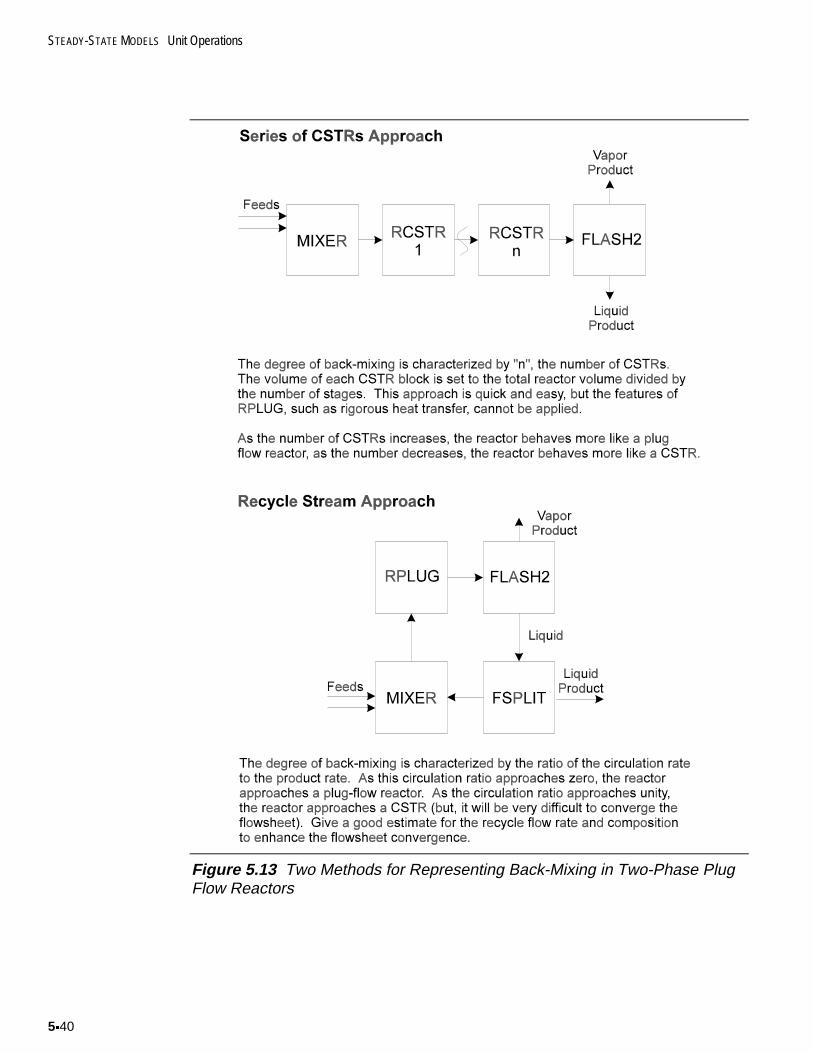
STEADY-STATE MODELS Unit Operations
5x40
Figure 5.13 Two Methods for Representing Back-Mixing in Two-Phase PlugFlow Reactors
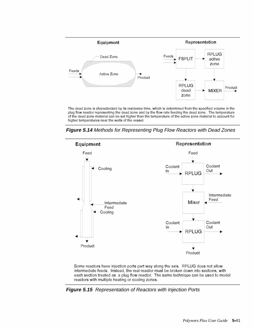
Polymers Plus User Guide 5x41
Figure 5.14 Methods for Representing Plug Flow Reactors with Dead Zones
Figure 5.15 Representation of Reactors with Injection Ports
STEADY-STATE MODELS Unit Operations
5x42
Troubleshooting Convergence Problems
To diagnose numerical problems in RPlug, set the terminal reporting level to “7” in theBlock-Options form. With this setting, the RPlug block will report the normalized axiallocation, residence time (in seconds), pressure (in Pascal), temperature (in K), and vapormolar fraction at each converged step.
The history level controls the diagnostic messages written to the history file (.HIS file).The maximum mass-balance error is reported at level 5. At level 6, the model reportsreacting component flow rates and component attribute values. At level 7, the model alsoreports the rates of change of these variables.
First, simplify the problem by specifying temperature instead of duty or heat-transferparameters (coolant temperature, U, or coolant stream). Specify the reactor as “liquid-only”. This will eliminate many possible sources of error and help focus the problem onkinetics and integration parameters.
Scaling Factors
RPlug uses Gear’s variable-step-size algorithm to numerically integrate the mass, energy,and attribute conservation equations along the axial dimension of the reactor. At eachaxial step, the conservation equations are solved by a trial-and-error technique.
Like RCSTR, RPlug solves the conservation equations using scaling factors to normalizethe variables. The values of these scaling factors can have a strong influence on the speedand reliability of the integration.
The Gear integrator in Aspen Plus offers two error scaling options (ERR-METHOD inRPlug), summarized in Table 5.6. The static scaling method uses a constant set of scalingfactors throughout the reactor. The dynamic scaling method updates the scaling factorsbased on the previously converged step. Both scaling methods conform to minimumscaling rules which are determined by a parameter called “cutoff”, which is analogous to“trace” in RCSTR.
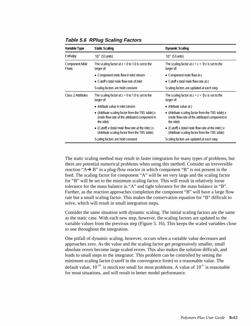
Polymers Plus User Guide 5x43
Table 5.6 RPlug Scaling Factors
Variable Type Static Scaling Dynamic Scaling
Enthalpy 105 (SI units) 105 (SI units)
Component MoleFlows
The scaling factor at z = 0 to 1.0 is set to thelarger of:
x Component mole flow in inlet stream
x Cutoff x total mole flow rate of inlet
Scaling factors are held constant
The scaling factor at z = z + �z is set to thelarger of:
x Component mole flow at z
x Cutoff x total mole flow rate at z
Scaling factors are updated at each step
Class 2 Attributes The scaling factor at z = 0 to 1.0 is set to thelarger of:
x Attribute value in inlet stream
x (Attribute scaling factor from the TBS table) x(mole flow rate of the attributed component inthe inlet)
x (Cutoff) x (total mole flow rate at the inlet ) x(Attribute scaling factor from the TBS table)
Scaling factors are held constant
The scaling factor at z = z + �z is set to thelarger of:
x Attribute value at z
x (Attribute scaling factor from the TBS table) x(mole flow rate of the attributed component inthe inlet)
x (Cutoff) x (total mole flow rate at the inlet ) x(Attribute scaling factor from the TBS table)
Scaling factors are updated at each step
The static scaling method may result in faster integration for many types of problems, butthere are potential numerical problems when using this method. Consider an irreversiblereaction “AÆ B” in a plug-flow reactor in which component “B” is not present in thefeed. The scaling factor for component “A” will be set very large and the scaling factorfor “B” will be set to the minimum scaling factor. This will result in relatively loosetolerance for the mass balance in “A” and tight tolerance for the mass balance in “B”.Further, as the reaction approaches completion the component “B” will have a large flowrate but a small scaling factor. This makes the conservation equation for “B” difficult tosolve, which will result in small integration steps.
Consider the same situation with dynamic scaling. The initial scaling factors are the sameas the static case. With each new step, however, the scaling factors are updated to thevariable values from the previous step (Figure 5. 16). This keeps the scaled variables closeto one throughout the integration.
One pitfall of dynamic scaling, however, occurs when a variable value decreases andapproaches zero. As the value and the scaling factor get progressively smaller, smallabsolute errors become large scaled errors. This also makes the solution difficult, andleads to small steps in the integrator. This problem can be controlled by setting theminimum scaling factor (cutoff in the convergence form) to a reasonable value. Thedefault value, 10-10 is much too small for most problems. A value of 10-5 is reasonablefor most situations, and will result in better model performance.
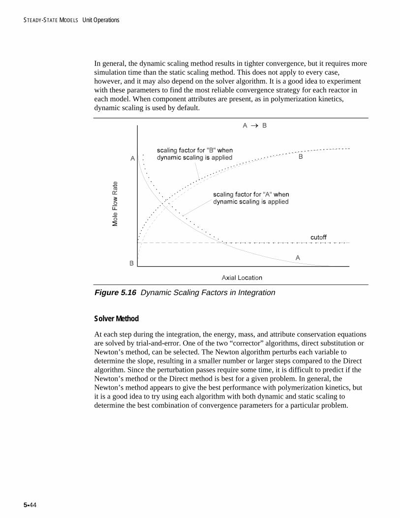
STEADY-STATE MODELS Unit Operations
5x44
In general, the dynamic scaling method results in tighter convergence, but it requires moresimulation time than the static scaling method. This does not apply to every case,however, and it may also depend on the solver algorithm. It is a good idea to experimentwith these parameters to find the most reliable convergence strategy for each reactor ineach model. When component attributes are present, as in polymerization kinetics,dynamic scaling is used by default.
Figure 5.16 Dynamic Scaling Factors in Integration
Solver Method
At each step during the integration, the energy, mass, and attribute conservation equationsare solved by trial-and-error. One of the two “corrector” algorithms, direct substitution orNewton’s method, can be selected. The Newton algorithm perturbs each variable todetermine the slope, resulting in a smaller number or larger steps compared to the Directalgorithm. Since the perturbation passes require some time, it is difficult to predict if theNewton’s method or the Direct method is best for a given problem. In general, theNewton’s method appears to give the best performance with polymerization kinetics, butit is a good idea to try using each algorithm with both dynamic and static scaling todetermine the best combination of convergence parameters for a particular problem.
Polymers Plus User Guide 5x45
The corrector tolerance is set as a ratio from the integration tolerance (Corr-Tol-Ratio).By default, the corrector tolerance is ten times tighter than the integration tolerance (thecorrector tolerance ratio is 0.1). For some problems, especially those involving reactorswith heat transfer calculations, the optimal corrector tolerance ratio may be higher than0.1, but this ratio should not be set larger than 1.0. The flash tolerance should be tighterthan the corrector tolerance. Otherwise, round-off errors in the flash calculations make thecorrector tolerance difficult to achieve. The model always uses the smaller of thespecified RPlug flash tolerance (in the convergence form) or the global flash tolerance.
Other Integration Parameters
By default, the initial step size in RPlug is set to one percent of the reactor length(Hinit=0.01). If the solver cannot converge the equations with this step size, it will cut thestep size by a factor of ten. This process will repeat up to six times. If the solver stillcannot converge, the reactor calculation fails with an error message “solver cannotconverge with minimum step size”.
Frequently, reaction rates or heat transfer rates are much faster near the entrance of thereactor than at the exit of a reactor due to step changes in temperature or pressure or dueto the high concentrations of reactants at the inlet of the reactor. For these types ofproblems, the minimum step size may need to be reduced. For step-growth kinetics, tryusing an initial step size of 1 10-4u . Smaller initial step-sizes may be required for additionkinetics, especially if quasi-steady-state approximations are not applied.
The maximum number of integration steps defaults to 1000. For very “stiff” kinetics, e.g.,kinetics with fast reaction rates involving trace components, the maximum number ofsteps may need to be increased, especially if the corrector is using direct substitution. Ifmore than 5000 steps are required, try changing the corrector method, scaling method, orincrease the cutoff level.
RPlug stores many types of results at regular intervals (printing points). The number ofintervals defaults to ten, but the number of print points can be increased to get smootherplots. Since the integration steps do not necessarily correspond to the print points, themodel uses polynomial interpolation to determine the results for a print point based on thesteps before and after this point. If the integration step sizes are very large, theinterpolation algorithm may give strange results, such as sine waves. This problem can befixed by reducing the maximum step size (Max-StepSize) to a value smaller than theincrements between print points (this forces the model to use linear interpolation). Bydefault, the maximum step size is much larger than the reactor length.
Summary
Table 5.7 summarizes common problems encountered when using the RPlug unitoperation block.
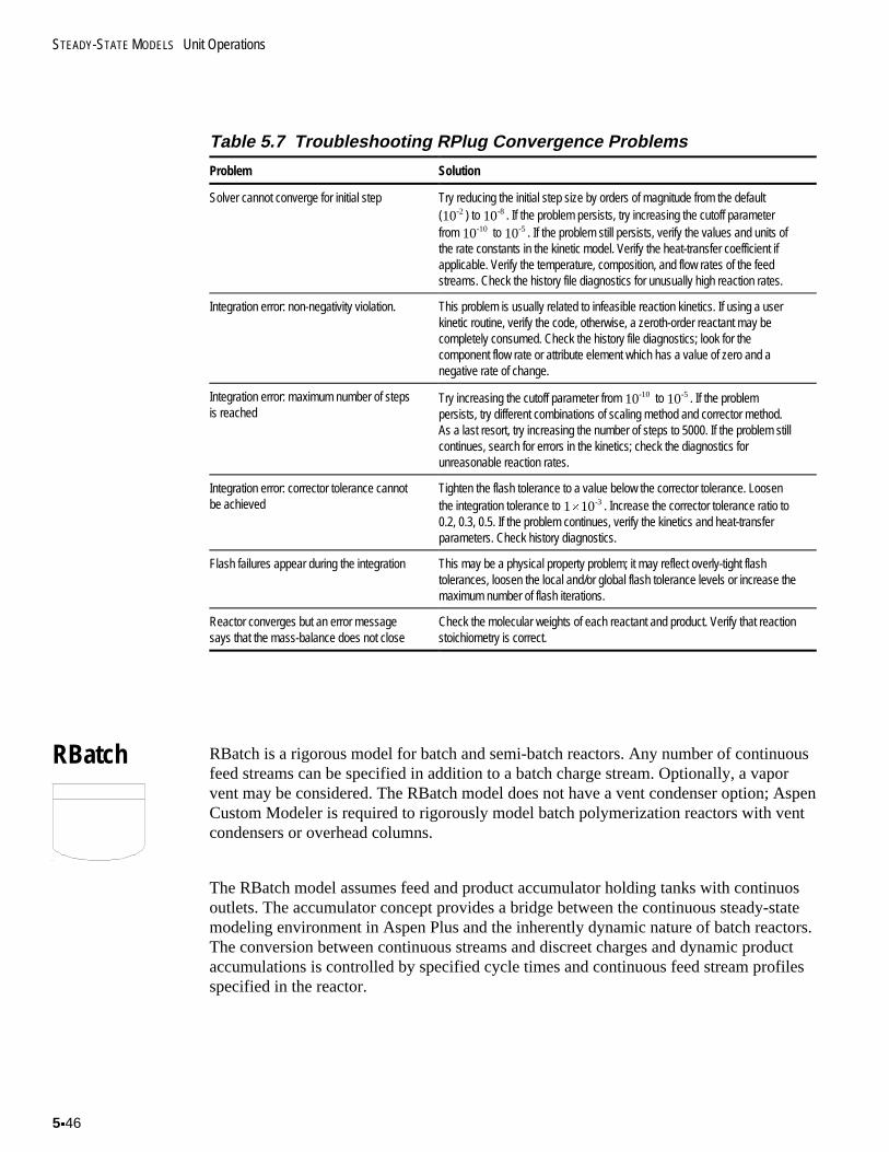
STEADY-STATE MODELS Unit Operations
5x46
Table 5.7 Troubleshooting RPlug Convergence Problems
Problem Solution
Solver cannot converge for initial step Try reducing the initial step size by orders of magnitude from the default(10-2 ) to 10-8 . If the problem persists, try increasing the cutoff parameterfrom 10-10 to 10-5 . If the problem still persists, verify the values and units ofthe rate constants in the kinetic model. Verify the heat-transfer coefficient ifapplicable. Verify the temperature, composition, and flow rates of the feedstreams. Check the history file diagnostics for unusually high reaction rates.
Integration error: non-negativity violation. This problem is usually related to infeasible reaction kinetics. If using a userkinetic routine, verify the code, otherwise, a zeroth-order reactant may becompletely consumed. Check the history file diagnostics; look for thecomponent flow rate or attribute element which has a value of zero and anegative rate of change.
Integration error: maximum number of stepsis reached
Try increasing the cutoff parameter from 10-10 to 10-5 . If the problempersists, try different combinations of scaling method and corrector method.As a last resort, try increasing the number of steps to 5000. If the problem stillcontinues, search for errors in the kinetics; check the diagnostics forunreasonable reaction rates.
Integration error: corrector tolerance cannotbe achieved
Tighten the flash tolerance to a value below the corrector tolerance. Loosenthe integration tolerance to 1 10-3
u . Increase the corrector tolerance ratio to0.2, 0.3, 0.5. If the problem continues, verify the kinetics and heat-transferparameters. Check history diagnostics.
Flash failures appear during the integration This may be a physical property problem; it may reflect overly-tight flashtolerances, loosen the local and/or global flash tolerance levels or increase themaximum number of flash iterations.
Reactor converges but an error messagesays that the mass-balance does not close
Check the molecular weights of each reactant and product. Verify that reactionstoichiometry is correct.
RBatch RBatch is a rigorous model for batch and semi-batch reactors. Any number of continuousfeed streams can be specified in addition to a batch charge stream. Optionally, a vaporvent may be considered. The RBatch model does not have a vent condenser option; AspenCustom Modeler is required to rigorously model batch polymerization reactors with ventcondensers or overhead columns.
The RBatch model assumes feed and product accumulator holding tanks with continuosoutlets. The accumulator concept provides a bridge between the continuous steady-statemodeling environment in Aspen Plus and the inherently dynamic nature of batch reactors.The conversion between continuous streams and discreet charges and dynamic productaccumulations is controlled by specified cycle times and continuous feed stream profilesspecified in the reactor.
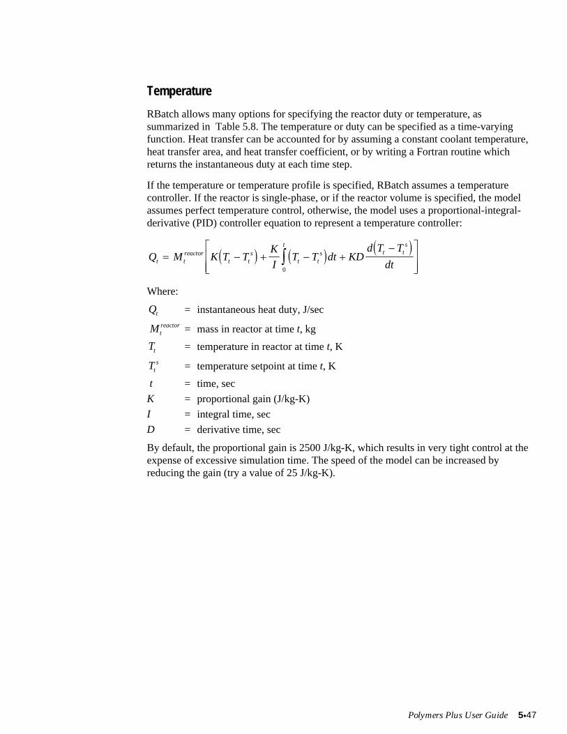
Polymers Plus User Guide 5x47
Temperature
RBatch allows many options for specifying the reactor duty or temperature, assummarized in Table 5.8. The temperature or duty can be specified as a time-varyingfunction. Heat transfer can be accounted for by assuming a constant coolant temperature,heat transfer area, and heat transfer coefficient, or by writing a Fortran routine whichreturns the instantaneous duty at each time step.
If the temperature or temperature profile is specified, RBatch assumes a temperaturecontroller. If the reactor is single-phase, or if the reactor volume is specified, the modelassumes perfect temperature control, otherwise, the model uses a proportional-integral-derivative (PID) controller equation to represent a temperature controller:
� � � �� �
Q M K T TK
IT T dt KD
d T T
dtt treactor
t ts
t ts t t
st
� � � ��ª
¬««
º
¼»»
³0
Where:
Qt = instantaneous heat duty, J/sec
Mtreactor = mass in reactor at time t, kg
Tt = temperature in reactor at time t, K
Tts = temperature setpoint at time t, K
t = time, sec
K = proportional gain (J/kg-K)
I = integral time, sec
D = derivative time, sec
By default, the proportional gain is 2500 J/kg-K, which results in very tight control at theexpense of excessive simulation time. The speed of the model can be increased byreducing the gain (try a value of 25 J/kg-K).
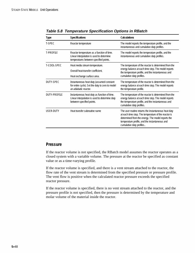
STEADY-STATE MODELS Unit Operations
5x48
Table 5.8 Temperature Specification Options in RBatch
Type Specifications Calculations
T-SPEC Reactor temperature The model reports the temperature profile, and theinstantaneous and cumulative duty profiles.
T-PROFILE Reactor temperature as a function of time.Linear interpolation is used to determinetemperatures between specified points.
The model reports the temperature profile, and theinstantaneous and cumulative duty profiles.
T-COOL-SPEC Heat media stream temperature.
Overall heat-transfer coefficient.
Heat exchange surface area.
The temperature of the reactor is determined from theenergy balance at each time step. The model reportsthe temperature profile, and the instantaneous andcumulative duty profiles.
DUTY-SPEC Instantaneous heat duty (assumed constantfor entire cycle). Set the duty to zero to modelan adiabatic reactor.
The temperature of the reactor is determined from theenergy balance at each time step. The model reportsthe temperature profile.
DUTY-PROFILE Instantaneous heat duty as function of time.Linear interpolation is used to determine dutybetween specified points.
The temperature of the reactor is determined from theenergy balance at each time step. The model reportsthe temperature profile, and the instantaneous andcumulative duty profiles.
USER-DUTY Heat transfer subroutine name The user routine returns the instantaneous heat dutyat each time step. The temperature of the reactor isdetermined from the energy. The model reports thetemperature profile, and the instantaneous andcumulative duty profiles..
Pressure
If the reactor volume is not specified, the RBatch model assumes the reactor operates as aclosed system with a variable volume. The pressure at the reactor be specified as constantvalue or as a time-varying profile.
If the reactor volume is specified, and there is a vent stream attached to the reactor, theflow rate of the vent stream is determined from the specified pressure or pressure profile.The vent flow is positive when the calculated reactor pressure exceeds the specifiedreactor pressure.
If the reactor volume is specified, there is no vent stream attached to the reactor, and thepressure profile is not specified, then the pressure is determined by the temperature andmolar volume of the material inside the reactor.
Polymers Plus User Guide 5x49
If the reactor volume is controlled, a pressure controller model can be linked to acontinuous feed stream. The flow rate of the feed stream is adjusted to maintain a constantpressure inside the vessel. The continuous feed stream flow rate can decrease to zero, butit cannot reverse direction if the pressure exceeds the specified setpoint. The model uses aproportional-integral-derivative (PID) controller equation to represent the pressurecontroller:
� � � �� �
F K P PK
IP P dt KD
d P P
dtt t ts
t ts
tt t
s
� � � ��ª
¬««
º
¼»»
³0
Where:
Ft = instantaneous flow rate, kmol/sec
Pt = pressure in reactor at time t, Pa
Pts = pressure setpoint at time t, Pa
t = time, sec
K = proportional gain (kmol/sec)/Pa
I = integral time, sec
D = derivative time, sec
Reactor Volume
If the reactor pressure is not specified, then RBatch will predict the reactor pressure basedon a specified reactor volume. The pressure will be manipulated by a trial-and-erroralgorithm to satisfy the specified volume.
If pressure and volume are both specified, you must either attach a vent stream to thereactor or attach a continuous make-up stream and pressure controller to the reactor.
Residence Time
The residence time of the reactor is controlled by user-specified stop criteria. You canspecify whether RBatch should halt the reaction when the stop criterion variable isapproached from above or below. If several stop criteria are specified, RBatch stops at thefirst stop criteria it reaches.
In addition to stop criteria, you must specify a maximum time for the reactor. Thisprevents runaway calculations in the event that none of the stop criteria are feasible.
STEADY-STATE MODELS Unit Operations
5x50
The stop criteria may include one or more of the following:
x A maximum reaction timex A maximum or minimum component mole or mass fraction in the reactorx The amount of material (mass, moles, or volume) in the reactor or vent accumulatorx A maximum vent flow ratex A maximum or minimum reactor temperature, pressure, or vapor fractionx The value of a Prop-Set property (includes user Prop-Set properties or system
properties such as viscosity, etc.)
Batch Operations
RBatch can represent batch or semi-batch reactors, depending on what streams areconnected to it in the flowsheet. If a vent stream or time-varying continuous feed stream isconnected to the RBatch block, then the model operates in semi-batch mode.
The batch reactor model is interfaced into the Aspen Plus continuous flow, steady-statemodeling environment through the concept of holding tanks, as shown in Figure 5.17. Theholding tanks convert the:
x Continuous batch charge stream to a discreet batch chargex Final vent accumulator inventory to a continuous, time-averaged vent streamx Final reactor inventory to a continuous, time-averaged reactor product stream
Figure 5.17 RBatch Reactor Configuration
Polymers Plus User Guide 5x51
Four types of streams are associated with RBatch:
x Continuous Batch Chargex Time-Varying Continuous Feedx Time-averaged Continuous Reactor Productx Time-averaged Continuous Vent Product
Continuous Batch Charge: The material transferred to the reactor at the start of the cycle.The mass of the batch charge equals the flow rate of the batch charge stream, multipliedby the batch cycle time. The mass of the batch charge is equivalent to accumulating thebatch charge stream in a holding tank during a reactor cycle. The contents of the batchcharge holding tank are instantaneously transferred to the reactor at the start of each batchcycle.
Time-Varying Continuous Feed: Streams which are fed to the reactor over some discreetinterval during the batch cycle. The composition, temperature, pressure, componentattribute values, and time-averaged flow rate of the stream are specified in the flowsheet.The flow rate of the continuous feed streams can be specified as a constant value, a time-varying profile, or manipulated by the pressure controller model to meet a time-varyingpressure setpoint.
Time-averaged Continuous Reactor Product: This stream is determined by dividing thefinal reactor inventory by the cycle time. This is analogous to instantaneously dumpingthe reactor contents to a large holding tank at the end of the cycle, and continuouslydraining the tank throughout each cycle.
Time-averaged Continuous Vent Product: This stream is determined by dividing thefinal vent accumulator inventory by the cycle time. During the batch cycle, the time-varying continuous vent stream is accumulated in the vent accumulator. The modelassumes the vent accumulator contents are instantly drained to a large holding tank at theend of the cycle, and the holding tank contents are continuously removed throughout thecycle.
Cycle Time
RBatch is a dynamic batch reactor model which is interfaced into the Aspen Pluscontinuous steady-state modeling environment. The interface requires converting batchcharges and accumulator inventories into continuous stream flow rates. The cycle time isused to convert the batch charge flow rate into the initial reactor inventory. The cycle timeis also used to convert the vent accumulator inventory and the reactor inventory into ventand reactor product streams.
STEADY-STATE MODELS Unit Operations
5x52
For example, assuming a reactor has a cycle time of two hours and that no continuousfeed streams are specified, then:
x If the batch charge stream is set to 50 kg/hour, the initial reactor inventory is 100 kg.x If at the end of the reaction cycle, the vent accumulator contains 30 kg of material, the
time-averaged continuous vent stream flow rate is 15 kg/hr. The composition of thetime-averaged vent stream will be the same as the final composition in the ventaccumulator.
x The final reactor inventory will be 70 kg, and the time-averaged reactor product flowrate will be 35 kg/hr.
RBatch allows you to specify a feed time and down time instead of the cycle time. In thiscase, the time-averaged batch charge stream is divided by the feed time to calculate theinitial batch inventory. The time-averaged product flow rates are based on the cycle time,which is calculated from the sum of the feed time, the down time, and the reaction time.This option is not recommended unless it is used to correct the mass balance for theinfluence of time-varying continuous feed streams.
Troubleshooting Convergence Problems
To diagnose numerical problems in RBatch, set the terminal reporting level to “7” in theBlock-Options form. With this setting, RBatch reports the time (in seconds), pressure (inPascal), temperature (in K), and vapor mole fraction at each converged integration step.
The history level controls the diagnostic messages written to the history file (.HIS file).The maximum mass-balance error is reported at level 5. At level 6, the model reportsreacting component flow rates and component attribute values. At level 7, the model alsoreports the rates of change of these variables.
First, simplify the problem by specifying temperature instead of duty or heat-transferparameters (coolant temperature, U, or heat transfer subroutine). Specify the reactor as“liquid-only”. Specify the reactor pressure, but not the reactor volume. This will eliminatemany possible sources of error and help focus the problem on kinetics and integrationparameters. Once the model works with these settings, then revert the settings to duty,volume, and so on, making sure the model converges with each new specification.
Scaling Factors
RBatch uses Gear’s variable-step-size algorithm to numerically integrate the mass,energy, and attribute conservation equations for the reactor and the mass-balanceequations for the vent condenser (if applicable). At each time step, the conservationequations are solved by a trial-and-error technique.
RBatch solves the conservation equations using scaling factors to normalize the variables.The values of these scaling factors have a strong influence on the speed and reliability ofthe integration.
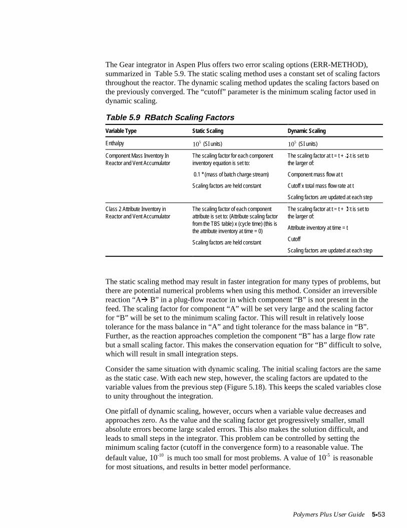
Polymers Plus User Guide 5x53
The Gear integrator in Aspen Plus offers two error scaling options (ERR-METHOD),summarized in Table 5.9. The static scaling method uses a constant set of scaling factorsthroughout the reactor. The dynamic scaling method updates the scaling factors based onthe previously converged. The “cutoff” parameter is the minimum scaling factor used indynamic scaling.
Table 5.9 RBatch Scaling Factors
Variable Type Static Scaling Dynamic Scaling
Enthalpy 105 (SI units) 105 (SI units)
Component Mass Inventory InReactor and Vent Accumulator
The scaling factor for each componentinventory equation is set to:
0.1 * (mass of batch charge stream)
Scaling factors are held constant
The scaling factor at t = t + �t is set tothe larger of:
Component mass flow at t
Cutoff x total mass flow rate at t
Scaling factors are updated at each step
Class 2 Attribute Inventory inReactor and Vent Accumulator
The scaling factor of each componentattribute is set to: (Attribute scaling factorfrom the TBS table) x (cycle time) (this isthe attribute inventory at time = 0)
Scaling factors are held constant
The scaling factor at t = t + �t is set tothe larger of:
Attribute inventory at time = t
Cutoff
Scaling factors are updated at each step
The static scaling method may result in faster integration for many types of problems, butthere are potential numerical problems when using this method. Consider an irreversiblereaction “AÆ B” in a plug-flow reactor in which component “B” is not present in thefeed. The scaling factor for component “A” will be set very large and the scaling factorfor “B” will be set to the minimum scaling factor. This will result in relatively loosetolerance for the mass balance in “A” and tight tolerance for the mass balance in “B”.Further, as the reaction approaches completion the component “B” has a large flow ratebut a small scaling factor. This makes the conservation equation for “B” difficult to solve,which will result in small integration steps.
Consider the same situation with dynamic scaling. The initial scaling factors are the sameas the static case. With each new step, however, the scaling factors are updated to thevariable values from the previous step (Figure 5.18). This keeps the scaled variables closeto unity throughout the integration.
One pitfall of dynamic scaling, however, occurs when a variable value decreases andapproaches zero. As the value and the scaling factor get progressively smaller, smallabsolute errors become large scaled errors. This also makes the solution difficult, andleads to small steps in the integrator. This problem can be controlled by setting theminimum scaling factor (cutoff in the convergence form) to a reasonable value. Thedefault value, 10-10 is much too small for most problems. A value of 10-5 is reasonablefor most situations, and results in better model performance.
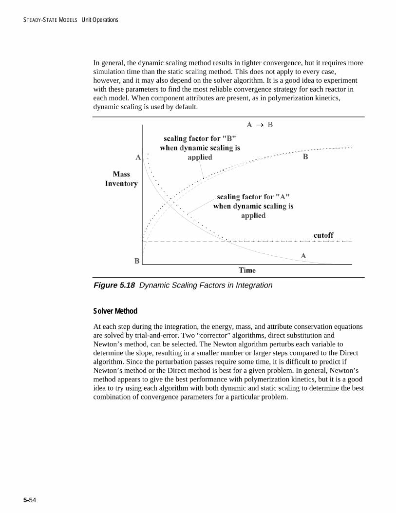
STEADY-STATE MODELS Unit Operations
5x54
In general, the dynamic scaling method results in tighter convergence, but it requires moresimulation time than the static scaling method. This does not apply to every case,however, and it may also depend on the solver algorithm. It is a good idea to experimentwith these parameters to find the most reliable convergence strategy for each reactor ineach model. When component attributes are present, as in polymerization kinetics,dynamic scaling is used by default.
Figure 5.18 Dynamic Scaling Factors in Integration
Solver Method
At each step during the integration, the energy, mass, and attribute conservation equationsare solved by trial-and-error. Two “corrector” algorithms, direct substitution andNewton’s method, can be selected. The Newton algorithm perturbs each variable todetermine the slope, resulting in a smaller number or larger steps compared to the Directalgorithm. Since the perturbation passes require some time, it is difficult to predict ifNewton’s method or the Direct method is best for a given problem. In general, Newton’smethod appears to give the best performance with polymerization kinetics, but it is a goodidea to try using each algorithm with both dynamic and static scaling to determine the bestcombination of convergence parameters for a particular problem.
Polymers Plus User Guide 5x55
The corrector tolerance is set as a ratio from the integration tolerance (Corr-Tol-Ratio).By default, the corrector tolerance is ten times tighter than the integration tolerance (thecorrector tolerance ratio is 0.1). For some problems, especially those involving reactorswith heat transfer calculations, the optimal corrector tolerance ratio may be higher than0.1, but this ratio should not be set larger than 1.0. The flash tolerance should be tighterthan the corrector tolerance. Otherwise, round-off errors in the flash calculations make thecorrector tolerance difficult to achieve. The model always uses the smaller of thespecified RPlug flash tolerance (in the convergence form) or the global flash tolerance.
Other Integration Parameters
By default, the initial step size in RBatch is set to one tenth of a second (Hinit=0.1). If thesolver cannot converge the equations with this step size, it will cut the step size by a factorof ten. This process will repeat up to six times. If the solver still cannot converge, thereactor fails with an error message “solver cannot converge with minimum step size”.
Frequently, initial reaction rates or heat transfer rates are very fast, so the minimum stepsize may need to be reduced. For step-growth kinetics, the default value should besufficient. Smaller initial step-sizes may be required for addition kinetics, especially ifquasi-steady-state approximations are not applied.
The maximum number of integration steps defaults to 1000. For very “stiff” kinetics, e.g.,kinetics with fast reaction rates involving trace components, the maximum number ofsteps may need to be increased, especially if the corrector is using direct substitution. Ifmore than 5000 steps are required, try changing the corrector method, scaling method, orincrease the cutoff level.
RBatch stores many types of results at regular intervals (printing points). The number ofintervals depends on the reaction time. Since the integration steps do not necessarilycorrespond to the print points, the model uses polynomial interpolation to determine theresults for a print point based on the steps before and after this point. If the integrationstep sizes are very large, the interpolation algorithm may give strange results, such as sinewaves. This problem can be fixed by reducing the maximum step size (Max-StepSize) toa value smaller than the increments between print points (this forces the model to uselinear interpolation). By default, no maximum step size is enforced.
RBatch has the option to stop exactly at print points and vent accumulator points insteadof interpolating these points. When the “exact” option is set to “yes”, the model adjuststhe integration steps to exactly match these points. This requires extra steps in theintegrator which may slow down the model, but it results in more accurate simulations.
Summary
Table 5.10 below summarizes common problems encountered when using RBatch.
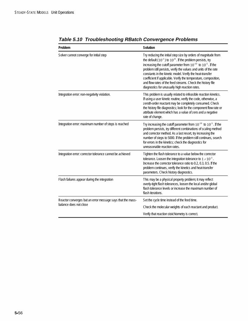
STEADY-STATE MODELS Unit Operations
5x56
Table 5.10 Troubleshooting RBatch Convergence Problems
Problem Solution
Solver cannot converge for initial step Try reducing the initial step size by orders of magnitude fromthe default (10-1 ) to 10-8 . If the problem persists, tryincreasing the cutoff parameter from 10-10 to 10-5 . If theproblem still persists, verify the values and units of the rateconstants in the kinetic model. Verify the heat-transfercoefficient if applicable. Verify the temperature, composition,and flow rates of the feed streams. Check the history filediagnostics for unusually high reaction rates.
Integration error: non-negativity violation. This problem is usually related to infeasible reaction kinetics.If using a user kinetic routine, verify the code, otherwise, azeroth-order reactant may be completely consumed. Checkthe history file diagnostics; look for the component flow rate orattribute element which has a value of zero and a negativerate of change.
Integration error: maximum number of steps is reached Try increasing the cutoff parameter from 10-10 to 10-5 . If theproblem persists, try different combinations of scaling methodand corrector method. As a last resort, try increasing thenumber of steps to 5000. If the problem still continues, searchfor errors in the kinetics; check the diagnostics forunreasonable reaction rates.
Integration error: corrector tolerance cannot be achieved Tighten the flash tolerance to a value below the correctortolerance. Loosen the integration tolerance to 1 10-3
u .Increase the corrector tolerance ratio to 0.2, 0.3, 0.5. If theproblem continues, verify the kinetics and heat-transferparameters. Check history diagnostics.
Flash failures appear during the integration This may be a physical property problem; it may reflectoverly-tight flash tolerances, loosen the local and/or globalflash tolerance levels or increase the maximum number offlash iterations.
Reactor converges but an error message says that the mass-balance does not close
Set the cycle time instead of the feed time.
Check the molecular weights of each reactant and product.
Verify that reaction stoichiometry is correct.
Polymers Plus User Guide 5x57
TREATMENT OF COMPONENT ATTRIBUTES IN UNIT OPERATIONMODELS
As described in previous chapters, Polymers Plus includes two classes of componentattributes. Class-2 attributes are “primary conserved quantities” and always have flow-typeunits (attribute value / unit time). These attributes include the zeroth moment of the polymer(polymer molecule flow rate), the segment flow rates, etc. Class-0 attributes are secondaryquantities which can be derived from the primary quantities.
The class-2 attributes follow flow-based mixing rules. In other words, if two streams aremixed, the product stream class-2 attributes are equal to the sum of the feed streamclass-2 attributes. These mixing rules apply to each unit operation which allows multiplefeeds of the same type (for example, multiple process fluid feeds). In the distillationmodels, these mixing rules apply on a tray-by-tray basis (e.g., if two or more feed streamsenter the same tray).
The blocks with more than one outlet (Flash2, Flash3, Sep, etc.) assume that the class 2polymer attributes split according to mass mixing rules. For example, if 90% of the massof the polymer flows to the liquid phase, then 90% of the polymer molecules also flowwith the liquid phase. This approach is identical to assuming that the properties of thepolymer, such as the molecular weight distribution, are not fractionated in any way;instead, the molecular weight distribution of each polymer component in each of theproduct phases is identical to that of the polymer in the feed stream. Table 5.11summarizes the attribute handling for the different models.
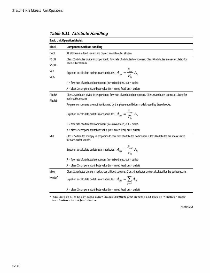
STEADY-STATE MODELS Unit Operations
5x58
Table 5.11 Attribute Handling
Basic Unit Operation Models
Block Component Attribute Handling
Dupl All attributes in feed stream are copied to each outlet stream.
FSplit
SSplit
Sep
Sep2
Class 2 attributes divide in proportion to flow rate of attributed component. Class 0 attributes are recalculated foreach outlet stream.
Equation to calculate outlet stream attributes: AF
FAout
out
inin
F = flow rate of attributed component (in = mixed feed, out = outlet)
A = class-2 component attribute value (in = mixed feed, out = outlet)
Flash2
Flash3
Class 2 attributes divide in proportion to flow rate of attributed component. Class 0 attributes are recalculated foreach outlet stream.
Polymer components are not fractionated by the phase equilibrium models used by these blocks.
Equation to calculate outlet stream attributes: AF
FAout
out
inin
F = flow rate of attributed component (in = mixed feed, out = outlet)
A = class-2 component attribute value (in = mixed feed, out = outlet)
Mult Class 2 attributes multiply in proportion to flow rate of attributed component. Class 0 attributes are recalculatedfor each outlet stream.
Equation to calculate outlet stream attributes: AF
FAout
out
inin
F = flow rate of attributed component (in = mixed feed, out = outlet)
A = class-2 component attribute value (in = mixed feed, out = outlet)
Mixer
Heater*
Class 2 attributes are summed across all feed streams. Class 0 attributes are recalculated for the outlet stream.
Equation to calculate outlet stream attributes: A Aout infeeds
¦
A = class-2 component attribute value (in = mixed feed, out = outlet)
* This also applies to any block which allows multiple feed streams and uses an “implied” mixerto calculate the net feed stream.
continued
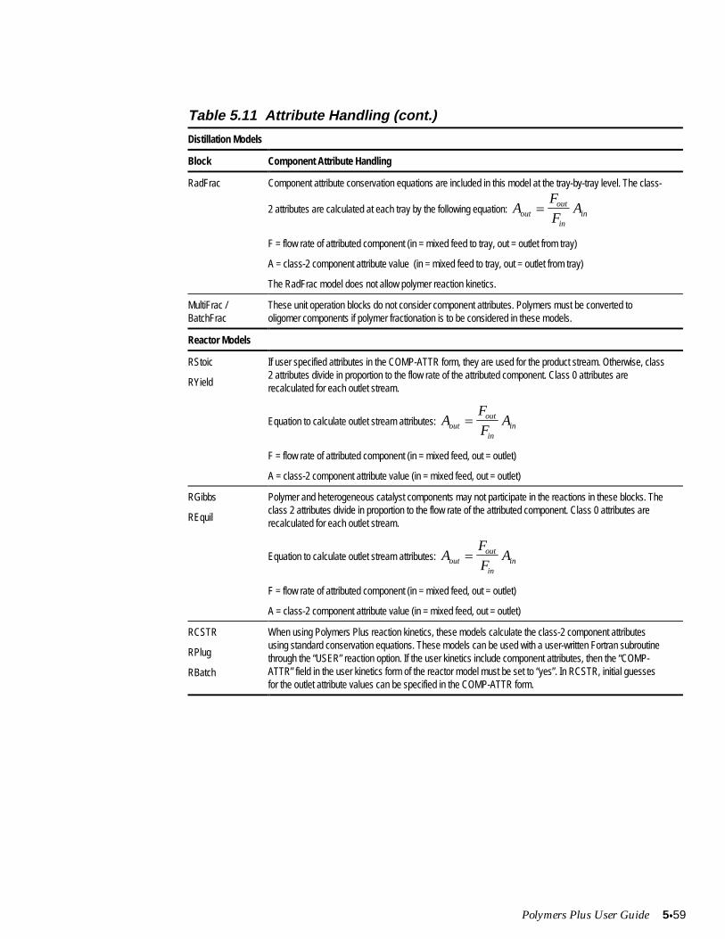
Polymers Plus User Guide 5x59
Table 5.11 Attribute Handling (cont.)
Distillation Models
Block Component Attribute Handling
RadFrac Component attribute conservation equations are included in this model at the tray-by-tray level. The class-
2 attributes are calculated at each tray by the following equation: AF
FAout
out
inin
F = flow rate of attributed component (in = mixed feed to tray, out = outlet from tray)
A = class-2 component attribute value (in = mixed feed to tray, out = outlet from tray)
The RadFrac model does not allow polymer reaction kinetics.
MultiFrac /BatchFrac
These unit operation blocks do not consider component attributes. Polymers must be converted tooligomer components if polymer fractionation is to be considered in these models.
Reactor Models
RStoic
RYield
If user specified attributes in the COMP-ATTR form, they are used for the product stream. Otherwise, class2 attributes divide in proportion to the flow rate of the attributed component. Class 0 attributes arerecalculated for each outlet stream.
Equation to calculate outlet stream attributes: AF
FAout
out
inin
F = flow rate of attributed component (in = mixed feed, out = outlet)
A = class-2 component attribute value (in = mixed feed, out = outlet)
RGibbs
REquil
Polymer and heterogeneous catalyst components may not participate in the reactions in these blocks. Theclass 2 attributes divide in proportion to the flow rate of the attributed component. Class 0 attributes arerecalculated for each outlet stream.
Equation to calculate outlet stream attributes: AF
FAout
out
inin
F = flow rate of attributed component (in = mixed feed, out = outlet)
A = class-2 component attribute value (in = mixed feed, out = outlet)
RCSTR
RPlug
RBatch
When using Polymers Plus reaction kinetics, these models calculate the class-2 component attributesusing standard conservation equations. These models can be used with a user-written Fortran subroutinethrough the “USER” reaction option. If the user kinetics include component attributes, then the “COMP-ATTR” field in the user kinetics form of the reactor model must be set to “yes”. In RCSTR, initial guessesfor the outlet attribute values can be specified in the COMP-ATTR form.
STEADY-STATE MODELS Unit Operations
5x60
REFERENCES
Chan, W.-M., P. E. Gloor, A. E. Hamielec, "A Kinetic Model for Olefin Polymerization inHigh-Pressure Autoclave Reactors," AIChE J., 39, No. 1 (1993).
Chaudhari, R. V., Y. T. Shah, Recent Advances in Slurry Reactors, Concepts and Designof Chemical Reactors, S.A. Whitaker and A. Cassano eds., Gordon and Breach SciencePublishers, Switzerland (1986).
Henderson, J. N., T. C. Bouton, eds., "Polymerization Reactors and Processes," ACSSymp. Ser., American Chemical Society (1979).
Rodriguez, F., Principles of Polymer Systems, Taylor & Francis, New York (1996).
Trambouze, P., H. van Landeghem, J. P. Wauquier, Chemical Reactors:Design/Engineering/Operation, Editions Technips, Paris (1988).
Walas, S. M., Chemical Process Equipment Selection and Design, Butterworths, Boston(1988).
Polymers Plus User Guide 5x61
5.2 PLANT DATA FITTING
Polymers Plus simulation models can be fit to plant or laboratory data using Data-Fit. Oneor more sets of measured data is provided which may include model inputs or results.Data-Fit adjusts or estimates input parameters to find the best match between the modelpredictions and data. Data-Fit can also reconcile measured data against the model.
Data-Fit minimizes the weighted sum of square errors, where each error is the differencebetween a reconciled input or calculated output and the data. In statistical terms, Data-Fitperforms either ordinary least squares or maximum likelihood (errors-in-variables)estimation.
Topics covered include:
x Data Fitting Applicationsx Data Fitting For Polymer Modelsx Steps in Using the Data Regression Tool (including troubleshooting tips)
This section emphasizes using the Data-Fit tool to fit process reaction kinetic parameters.A more general description of this tool is available in the Aspen Plus Reference Manual.
5.2
STEADY-STATE MODELS Data Fitting
5x62
DATA FITTING APPLICATIONS
The data regression tool in Aspen Plus can be used to fit model parameters and reconcileprocess data. These applications may be carried out simultaneously.
Parameter regression usually involves adjusting model parameters to improve theagreement between model predictions and process data. For example, process rateconstants may be manipulated to match the measured polymer molecular weight andmonomer conversion. Manipulated parameters may include reaction rate or equilibriumconstants, physical property constants, or equipment specifications. Fitted parameters mayinclude model predictions such as reactant conversion, product yield, by-product content,polymer component attributes, stream compositions or flow rates, or equipment heat duty,temperature, pressure, or holdup.
Data reconciliation runs involve manipulating one or more sets of model inputs to matchmodel predictions to process data. For example, the average feed rate of a makeup streamcan be estimated based on the flow rate and composition of the feed and product streams.Manipulated data typically includes feed stream flow rates and compositions, equipmentoperating conditions, heat transfer coefficients, etc.
The Data-Fit model can be used to reconcile input data and fit model parameterssimultaneously. Simultaneous regression and reconciliation is typically used to fine-tunemodels which already match process data and trends relatively well.
Polymers Plus User Guide 5x63
DATA FITTING FOR POLYMER MODELS
Polymer process models frequently include non-ideal phase equilibrium, reaction kinetics,and complicated unit operations. Fitting these complex models against process andlaboratory data is not a trivial task. A great deal of consideration must be given to the waythis problem is approached.
A detailed example describing how to fit a free-radical reaction kinetics problem isincluded in the Polymers Plus Examples & Applications Case Book.
A general procedure for fitting complex models is given below.
Step1. Process Data Review
Collect data for the process. Sources of data include process information managementsystem (PIMS), process design documents (PDDs), process flow diagrams (PFDs). Verifyreproducibility / standard deviations of data by collecting multiple data sets for each case.Verify steady state by collecting data at regular intervals over several plant residencetimes. Verify data feasibility against mass and energy balance calculations.
Step 2. Literature Search
Collect information about the process. Sources of data include in-house lab data,databanks, trade journals, conference notes, polymer handbooks, on-line electronicdatabases, experimental designs, etc.
Step 3. Preliminary Model Fitting
Carry out physical property data regression, property constant parameter estimation runs.Test the parameters against all pertinent data from steps 1 and 2. To the extent possible,verify pure component physical properties and phase equilibrium predictions usingProperty Analysis tools.
Step 4. Preliminary Model Development
Develop a basic model of the process, ignoring details such as non-ideal mixing, heattransfer, etc. Specify temperature instead of duty, volume instead of residence time. Useparameters from steps 1-3.
STEADY-STATE MODELS Data Fitting
5x64
Step 5. Trend Analysis
Use the sensitivity feature to evaluate trends between model outputs (conversion, polymerattributes, etc.) and model inputs (rate constants, operating conditions, etc.) Compare thepredicted trends against available process or lab data. If the trends are not well matched,adjust specific model parameters to improve the predicted trend. Model fitting may becarried out using Sensitivity, Design-Specification, Data-Fit, or by trial and error.
Step 6. Model Refinement
Use the Data-Fit tool to carry out simultaneous parameter estimation and datareconciliation. Relax model assumptions, such as perfect mixing, as needed. Bring modelup to the appropriate level of detail, fitting key parameters at each development step.
DataCollectionandVerification
The first step in fitting a model is to collect and review data. Sources of data may includeprocess information management system (PIMS), process design documents (PDDs), andprocess flow diagrams (PFDs), shift log sheets, and laboratory analysis reports. It isimportant to verify the reproducibility of the data by collecting several duplicate sets ofeach datum. Duplicate data are especially important for analytical measurements such asmelt flow index and intrinsic viscosity.
For continuous processes, it is a good idea to verify that the process operates understeady-state conditions by collecting data at regular intervals. The data should becollected at regular intervals over a period which exceeds the cumulative residence timeof the key unit operations in the process.
Verify data feasibility against mass and energy balance calculations. It is impossible toforce a rigorous model to match data which violates the fundamental conservationequations.
When possible, obtain calibration data for unit operating conditions, especially levelcalibration data for reactors and flow rate calibration data for flow meters. The methodand assumptions used to calibrate these instruments must be taken into consideration fordata reconciliation runs.
Polymers Plus User Guide 5x65
LiteratureReview
Before you regress process data, it is a good idea to collect information about the process.Sources of data include in-house lab data, databanks, trade journals, conference notes,polymer handbooks, on-line electronic databases, experimental designs, and so on.
The open and in-house process literature may contain a wealth of information about keymodel parameters. Further, these sources may provide additional sources of fundamentaldata which can be used to independently evaluate model parameters.
Simulation studies described in trade journals are an excellent source of insight andknow-how related to model development. These studies frequently point out whichassumptions are valid and which parameters are important. In addition, these papers mayelucidate reaction mechanisms or physical phenomena which should be considered in arigorous process model.
The physical property and rate constant data reported in the open literature are neverperfect, but they do serve as a good starting point for fitting the model.
PreliminaryParameterFitting
It is important to determine as many of the model parameters as possible early in themodel development process. Try to decouple the parameters from each other wheneverpossible. For example, find ways to establish phase equilibrium parameters independentlyof reaction equilibrium constants. Make simplifying assumptions to reduce the number ofunknown parameters.
Physical property parameters should be firmly established before fitting rate constants.When data are available, use the physical property data regression system (DRS) to fit thedensity, enthalpy, heat capacity, and vapor pressure of pure components. If phaseequilibrium data are available, use DRS to regress phase equilibrium parameters.
When property data are unavailable for a component, the property constant estimationsystem (PCES) can be used to estimate property parameters from molecular structure.These estimations, however, should be checked against process data. If data are availablefor components with similar structures, they can be used to estimate the properties ofcomponents which are not found in the databank.
Table 5.12 lists some of the key physical property parameters in Polymers Plus anddescribes how they influence polymerization kinetics.
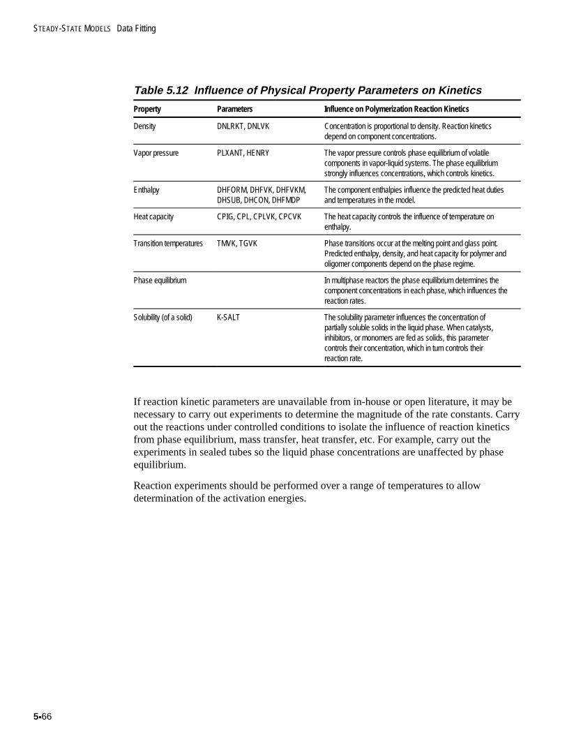
STEADY-STATE MODELS Data Fitting
5x66
Table 5.12 Influence of Physical Property Parameters on Kinetics
Property Parameters Influence on Polymerization Reaction Kinetics
Density DNLRKT, DNLVK Concentration is proportional to density. Reaction kineticsdepend on component concentrations.
Vapor pressure PLXANT, HENRY The vapor pressure controls phase equilibrium of volatilecomponents in vapor-liquid systems. The phase equilibriumstrongly influences concentrations, which controls kinetics.
Enthalpy DHFORM, DHFVK, DHFVKM,DHSUB, DHCON, DHFMDP
The component enthalpies influence the predicted heat dutiesand temperatures in the model.
Heat capacity CPIG, CPL, CPLVK, CPCVK The heat capacity controls the influence of temperature onenthalpy.
Transition temperatures TMVK, TGVK Phase transitions occur at the melting point and glass point.Predicted enthalpy, density, and heat capacity for polymer andoligomer components depend on the phase regime.
Phase equilibrium In multiphase reactors the phase equilibrium determines thecomponent concentrations in each phase, which influences thereaction rates.
Solubility (of a solid) K-SALT The solubility parameter influences the concentration ofpartially soluble solids in the liquid phase. When catalysts,inhibitors, or monomers are fed as solids, this parametercontrols their concentration, which in turn controls theirreaction rate.
If reaction kinetic parameters are unavailable from in-house or open literature, it may benecessary to carry out experiments to determine the magnitude of the rate constants. Carryout the reactions under controlled conditions to isolate the influence of reaction kineticsfrom phase equilibrium, mass transfer, heat transfer, etc. For example, carry out theexperiments in sealed tubes so the liquid phase concentrations are unaffected by phaseequilibrium.
Reaction experiments should be performed over a range of temperatures to allowdetermination of the activation energies.
Polymers Plus User Guide 5x67
PreliminaryModelDevelopment
Once the preliminary parameter fitting is complete, these parameters can be used todevelop a preliminary model. At this stage of the model development process, it may bebest to use simplified models for some of the ancillary operations which are not directlyinvolved in the polymerization reactors. For example, it may be more convenient torepresent distillation columns using the non-predictive Sep or Sep2 models instead of theRadFrac or MultiFrac rigorous distillation models.
The most important rule for model development is to “keep it simple”. Modeldevelopment must be carried out in several stages. Add detail to the model one step at atime. Each generation of the model can yield valuable insights into the process and canprovide substantial benefit to the model developer. At each stage in the process, fit theappropriate model parameters and validate the model against all sources of available data.Verify the predicted trends against process data, operator experience, and engineeringknow-how. Over time, the level of detail and power of the model can be increased.
During the preliminary development, use the most basic specifications possible. Forexample, in the RCSTR model specify temperature and reacting phase volume instead ofduty and residence time. This approach will make the model run faster and will help toisolate the influence of property parameters from reaction kinetic parameters.
Once the preliminary model is complete, it can be tested against process data. Majordiscrepancies between the data and the model predictions should be addressed during thisstep.
TrendAnalysis
Use the preliminary model to carry out trend evaluation studies. The sensitivity featurecan be used to examine the influence of process variables on the model predictions.Compare these trends against process data. If the predicted trends are not consistent,adjust the appropriate model parameters to improve the match. For example, if thepredicted slope of the monomer conversion versus temperature curve is less than themeasured slope, the activation energy of the polymerization reaction may be too low.
Use the sensitivity tool to examine the influence of the model parameters on the modelpredictions and to determine which parameters are important in the model. Parametricstudies can be carried out by manipulating two or more variables in a sensitivity study.
It is good practice to include as many model predictions as possible in each sensitivitystudy. The simulation runs take the same amount of time regardless of the number ofdefined variables. It is much easier to understand the predicted trends when the sensitivityresults are detailed.
Once you know which parameters are critical to the model predictions, the data regressiontool can be used to adjust these parameters to match specific trends. Keep the number ofmanipulated parameters to a minimum until all of the key parameters are establishedindependently.
STEADY-STATE MODELS Data Fitting
5x68
ModelRefinement
The Data-Fit tool is the best choice for refining the fit between the model predictions andthe process data, especially when several sets of data are available. Data-Fit can adjustseveral model parameters simultaneously, capturing subtle interactions among theparameters to get the best overall match between the process data and model predictions.
When the model predictions cannot match the process data, the assumptions in the modelmay be too broad. Perhaps the process is limited by heat- or mass-transfer, or a reactor isnot ideally mixed. Maybe there are additional side reactions which should be consideredin the model, or the rate expression needs to be modified to account for some unusualaspect of reaction kinetics. These issues can be addressed during the model refinementprocess by adding new layers of detail to the model. Avoid adding more detail thannecessary, however, because model fitting is a process of diminishing returns.
Model refinement is an open-ended process. The model parameters can be tuned moreaccurately as more data become available from the process. Bad data points are easier tospot when there are more sets of data to compare.
It is impossible for a simulation model to match process data perfectly. There are severalsources of error that lead to differences between the model results and process data,including:
x Variations in process operating conditions due to disturbances, excursions from steadystate, control system actions, etc.
x Imperfect calibration of flow meters, level controllers, etc.x Analytical error in lab measurementsx Simplifications and assumptions in the model, such as ideal mixing, isothermal and
isobaric vessels, phase equilibrium, etc.x Errors in the model parameters.
Polymers Plus User Guide 5x69
STEPS IN USING THE DATA REGRESSION TOOL
There are three steps involved in using the data regression tool:
x Creating a base-case modelx Entering lab or process data and operating conditions into data setsx Defining regression cases
Step 1. Creating a base-case model
If the regression tool is being used to fit reaction kinetic parameters from lab batch reactordata, use the RBatch model with an appropriate reaction kinetic model.
If the model parameters are being regressed from process data, develop a model of theprocess. Before setting up the data fit run, make sure the model predictions are reasonableand that the model is robust (converges without errors) over the ranges of eachmanipulated parameter. You can use sensitivity blocks to screen the model for accuracyand to test how robust the model is.
The rate constants and property parameters entered into the base case model become theinitial estimates for the regression.
Step 2. Entering lab or process data and operating conditions into data sets
There are two types of data sets used with the regression tool, “Point-Data” and “Profile-Data”:
Use To specify
Point-Data x Operating conditions for steady-state unit operation models.
x Feed streams for continuous processes or batch charge streams.
x Analytical data, measured flow rates, or composition data for product streams.
x Polymer or catalyst component attribute data for product streams.
Profile-Data x Operating profiles for batch reactors or plug-flow reactors, including temperature, pressure, and dutyprofiles, continuous feed stream profiles, etc.
x Time-series measured data for a batch reactor or data along the axial profile of a plug-flow reactor.
x Note: Component attribute profiles and user variable profiles are not available as profile data in thisrelease of Polymers Plus. To fit profile data for these types of variables, treat each data point in theprofile as a point datum, and specify the coinciding stop-time (RBatch) or length (RPlug) of the reactoras another point datum in the same data set.
STEADY-STATE MODELS Data Fitting
5x70
Step 3. Defining regression cases
For each case, specify the parameters to be adjusted and the data sets to be fitted. Severalregression cases can be included in the same simulation run. The cases are runsequentially; a prompt will appear on the screen which allows you to specify which casesto include in the run, and the sequence order of the cases. Each successive case uses thefitted parameters and reconciled data from the previous case. If the data regression is runagain, the previously fit values are used as initial estimates unless the simulation isreinitialized.
IdentifyingFlowsheetVariables
You must identify each measured and manipulated variable considered in the regression.Most types of variables, such as stream flow rates, equipment operating conditions, andcomponent attribute values can be accessed directly using the variable accessing system..
In the data regression and data set forms, you cannot access vector data, such as thestream vector and component attribute vector. You must access each stream variable orcomponent attribute element as a separate scalar variable.
When specifying feed stream data, avoid using mole, mass, or volume fractions asvariables in the data set. If the composition of the feed stream changes from onevalidation case to another, specify the flow rates of the components in the stream. If thecomposition is constant but the flow rate changes, specify the composition and base-caseflow rate in the model, and specify the total stream flow rate as a point-data variable. Thisavoids problems with normalizing fractions and reduces the number of variables handledby the data-fit algorithm.
Some unit operation models have both input and results variables for the same operatingcondition. For example, in the RCSTR model you can access the specified heat duty(DUTY), or the calculated reactor duty (QCALC). If a variable is an INPUT variable inthe regression it must be specified in the unit operation model.
For example, if the reactor duty is a manipulated INPUT variable in the regression, itmust be specified as an input variable (DUTY), and the reactor duty must be specified inthe reactor model. If the reactor duty is a measured RESULTS variable, it must bespecified as a results variable (QCALC), and is usually not specified in the model (thetemperature is specified instead). Table 5.13 provides a cross-reference of commonly-used INPUT and RESULTS variables for key specifications related to several unitoperation models.
Some measured data, such as polymer melt index and intrinsic viscosity, are not predictedby the standard property sets in Polymers Plus. The best way to include these properties ina data regression is to write a user Prop-Set property subroutine. Each user property canbe linked to a property set. Property sets can be accessed as stream-property variables.
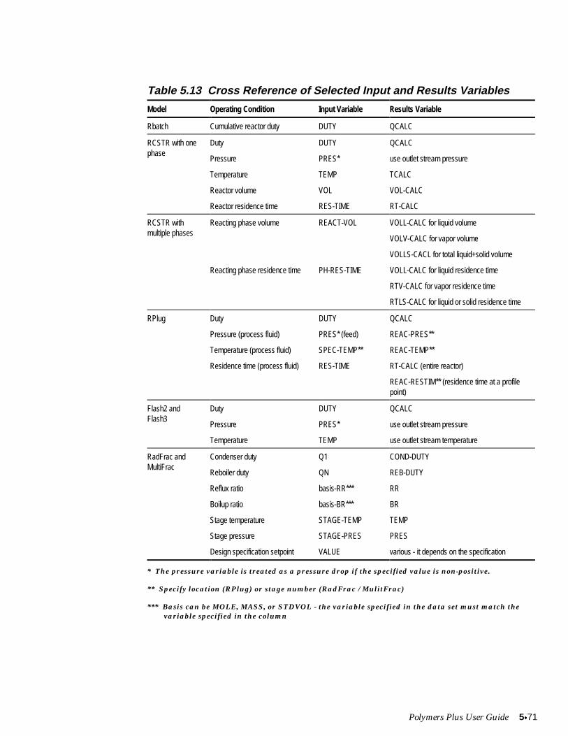
Polymers Plus User Guide 5x71
Table 5.13 Cross Reference of Selected Input and Results Variables
Model Operating Condition Input Variable Results Variable
Rbatch Cumulative reactor duty DUTY QCALC
RCSTR with onephase
Duty
Pressure
Temperature
Reactor volume
Reactor residence time
DUTY
PRES*
TEMP
VOL
RES-TIME
QCALC
use outlet stream pressure
TCALC
VOL-CALC
RT-CALC
RCSTR withmultiple phases
Reacting phase volume REACT-VOL VOLL-CALC for liquid volume
VOLV-CALC for vapor volume
VOLLS-CACL for total liquid+solid volume
Reacting phase residence time PH-RES-TIME VOLL-CALC for liquid residence time
RTV-CALC for vapor residence time
RTLS-CALC for liquid or solid residence time
RPlug Duty
Pressure (process fluid)
Temperature (process fluid)
Residence time (process fluid)
DUTY
PRES* (feed)
SPEC-TEMP**
RES-TIME
QCALC
REAC-PRES**
REAC-TEMP**
RT-CALC (entire reactor)
REAC-RESTIM** (residence time at a profilepoint)
Flash2 andFlash3
Duty
Pressure
Temperature
DUTY
PRES*
TEMP
QCALC
use outlet stream pressure
use outlet stream temperature
RadFrac andMultiFrac
Condenser duty
Reboiler duty
Reflux ratio
Boilup ratio
Stage temperature
Stage pressure
Design specification setpoint
Q1
QN
basis-RR***
basis-BR***
STAGE-TEMP
STAGE-PRES
VALUE
COND-DUTY
REB-DUTY
RR
BR
TEMP
PRES
various - it depends on the specification
* The pressure variable is treated as a pressure drop if the specified value is non-positive.
** Specify location (RPlug) or stage number (RadFrac / MulitFrac)
*** Basis can be MOLE, MASS, or STDVOL - the variable specified in the data set must match thevariable specified in the column
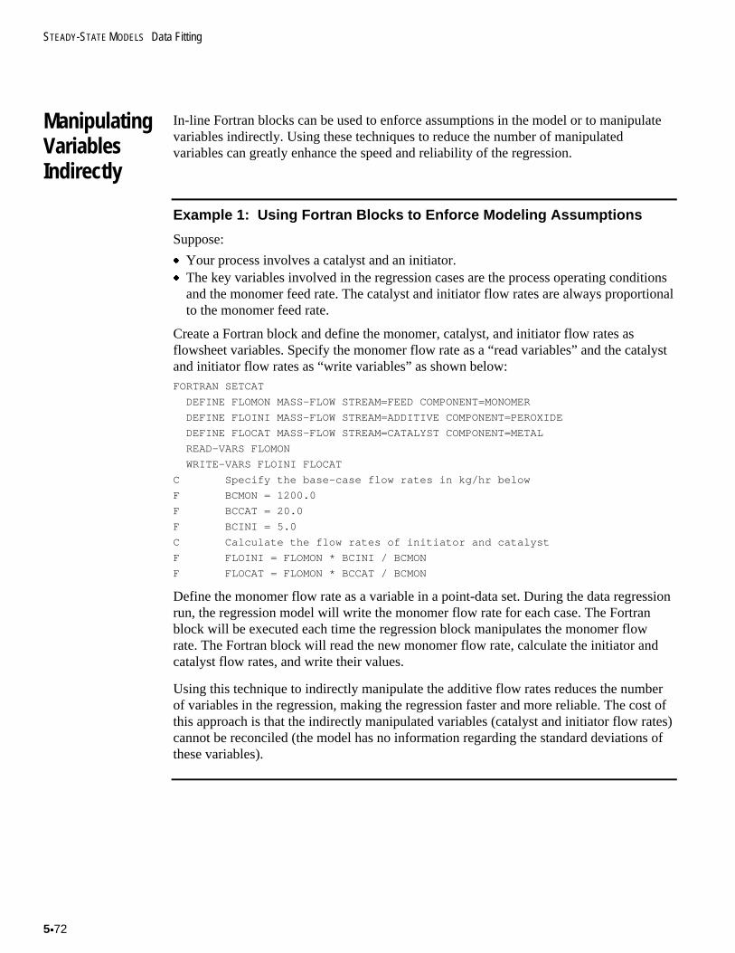
STEADY-STATE MODELS Data Fitting
5x72
ManipulatingVariablesIndirectly
In-line Fortran blocks can be used to enforce assumptions in the model or to manipulatevariables indirectly. Using these techniques to reduce the number of manipulatedvariables can greatly enhance the speed and reliability of the regression.
Example 1: Using Fortran Blocks to Enforce Modeling Assumptions
Suppose:
x Your process involves a catalyst and an initiator.x The key variables involved in the regression cases are the process operating conditions
and the monomer feed rate. The catalyst and initiator flow rates are always proportionalto the monomer feed rate.
Create a Fortran block and define the monomer, catalyst, and initiator flow rates asflowsheet variables. Specify the monomer flow rate as a “read variables” and the catalystand initiator flow rates as “write variables” as shown below:FORTRAN SETCAT
DEFINE FLOMON MASS-FLOW STREAM=FEED COMPONENT=MONOMER
DEFINE FLOINI MASS-FLOW STREAM=ADDITIVE COMPONENT=PEROXIDE
DEFINE FLOCAT MASS-FLOW STREAM=CATALYST COMPONENT=METAL
READ-VARS FLOMON
WRITE-VARS FLOINI FLOCAT
C Specify the base-case flow rates in kg/hr below
F BCMON = 1200.0
F BCCAT = 20.0
F BCINI = 5.0
C Calculate the flow rates of initiator and catalyst
F FLOINI = FLOMON * BCINI / BCMON
F FLOCAT = FLOMON * BCCAT / BCMON
Define the monomer flow rate as a variable in a point-data set. During the data regressionrun, the regression model will write the monomer flow rate for each case. The Fortranblock will be executed each time the regression block manipulates the monomer flowrate. The Fortran block will read the new monomer flow rate, calculate the initiator andcatalyst flow rates, and write their values.
Using this technique to indirectly manipulate the additive flow rates reduces the numberof variables in the regression, making the regression faster and more reliable. The cost ofthis approach is that the indirectly manipulated variables (catalyst and initiator flow rates)cannot be reconciled (the model has no information regarding the standard deviations ofthese variables).
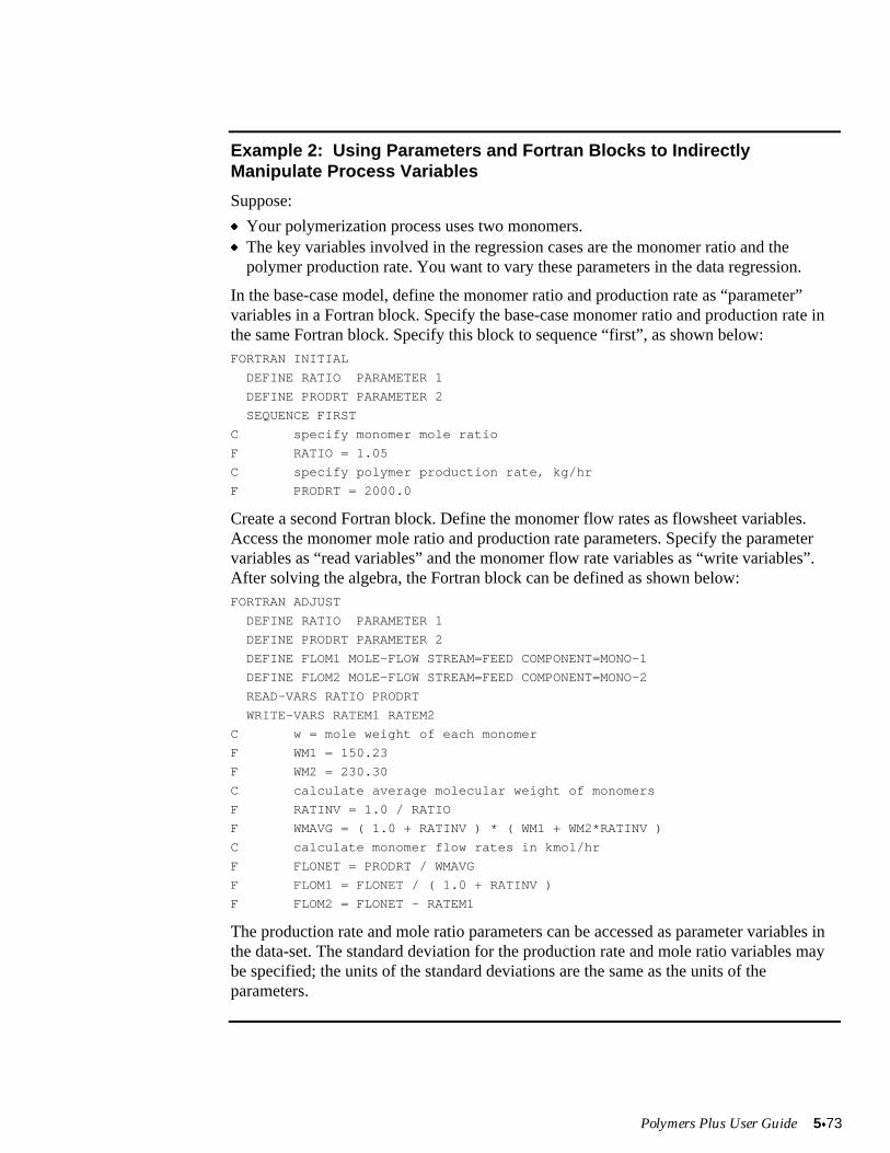
Polymers Plus User Guide 5x73
Example 2: Using Parameters and Fortran Blocks to IndirectlyManipulate Process Variables
Suppose:
x Your polymerization process uses two monomers.x The key variables involved in the regression cases are the monomer ratio and the
polymer production rate. You want to vary these parameters in the data regression.
In the base-case model, define the monomer ratio and production rate as “parameter”variables in a Fortran block. Specify the base-case monomer ratio and production rate inthe same Fortran block. Specify this block to sequence “first”, as shown below:FORTRAN INITIAL
DEFINE RATIO PARAMETER 1
DEFINE PRODRT PARAMETER 2
SEQUENCE FIRST
C specify monomer mole ratio
F RATIO = 1.05
C specify polymer production rate, kg/hr
F PRODRT = 2000.0
Create a second Fortran block. Define the monomer flow rates as flowsheet variables.Access the monomer mole ratio and production rate parameters. Specify the parametervariables as “read variables” and the monomer flow rate variables as “write variables”.After solving the algebra, the Fortran block can be defined as shown below:FORTRAN ADJUST
DEFINE RATIO PARAMETER 1
DEFINE PRODRT PARAMETER 2
DEFINE FLOM1 MOLE-FLOW STREAM=FEED COMPONENT=MONO-1
DEFINE FLOM2 MOLE-FLOW STREAM=FEED COMPONENT=MONO-2
READ-VARS RATIO PRODRT
WRITE-VARS RATEM1 RATEM2
C w = mole weight of each monomer
F WM1 = 150.23
F WM2 = 230.30
C calculate average molecular weight of monomers
F RATINV = 1.0 / RATIO
F WMAVG = ( 1.0 + RATINV ) * ( WM1 + WM2*RATINV )
C calculate monomer flow rates in kmol/hr
F FLONET = PRODRT / WMAVG
F FLOM1 = FLONET / ( 1.0 + RATINV )
F FLOM2 = FLONET - RATEM1
The production rate and mole ratio parameters can be accessed as parameter variables inthe data-set. The standard deviation for the production rate and mole ratio variables maybe specified; the units of the standard deviations are the same as the units of theparameters.
STEADY-STATE MODELS Data Fitting
5x74
EnteringPoint Data
There are two types of point data: input variables and result variables. Input variablesinclude feed stream flow rates, equipment operating conditions, and other parameterswhich are inputs to the simulation model. Result variables include product stream flowrates or composition, polymer or catalyst component attributes, stream properties, or anyother simulation calculation which can be compared to measured process data.
If some results data are missing from one or more sets of data, they can be left blank onthe input forms. The model will estimate the values of these results and tabulate themafter the regression run.
Unknown input data may also be estimated. Leave the input field blank and specify largestandard deviations (for example, 50%) for each missing datum. Supply a realistic initialguess and make sure the standard deviation results in reasonable bounds for each missingvariable.
The upper and lower bounds for reconciled unknown input variables are determined fromthe specified standard deviation and the “bound factor”, which defaults to ten:
Lower bound = Measured value - (Bound Factor)*(Standard Deviation)
Upper bound = Measured value + (Bound Factor)*(Standard Deviation)
Make sure these limits are reasonable. In particular, the limits for a stream flow rate mustnot allow the stream flow rate to become zero or negative.
EnteringProfile Data
The plug-flow reactor model (RPlug) predicts results at various points along its lengthaxis. The batch reactor model (RBatch) predicts results at various points in time duringthe batch cycle. You can define profile data sets to specify the operating profiles as inputdata, or to fit the model to measured results data.
To do this, specify the time and value for each datum in the profile. You can specifystandard deviations for results variables. Data reconciliation is not allowed for inputprofile data.
Table 5.14 lists the profile data sets which are currently available for these reactormodels. Other types of profiles, including component attribute, user variable, and userProp-Set property profiles are planned for a future releases of Polymers Plus.
If you are fitting component attribute or user Prop-Set property profiles, you must treat themeasured variables as point data for the reactor outlet stream. Use the reactor length orstop-time as an additional point data. Each profile point must be treated as a separate datacase in the data set.
If some results data are missing from one or more sets of profile data, they can be leftblank on the input forms. The model will estimate the values of these results and tabulatethem after the regression run.
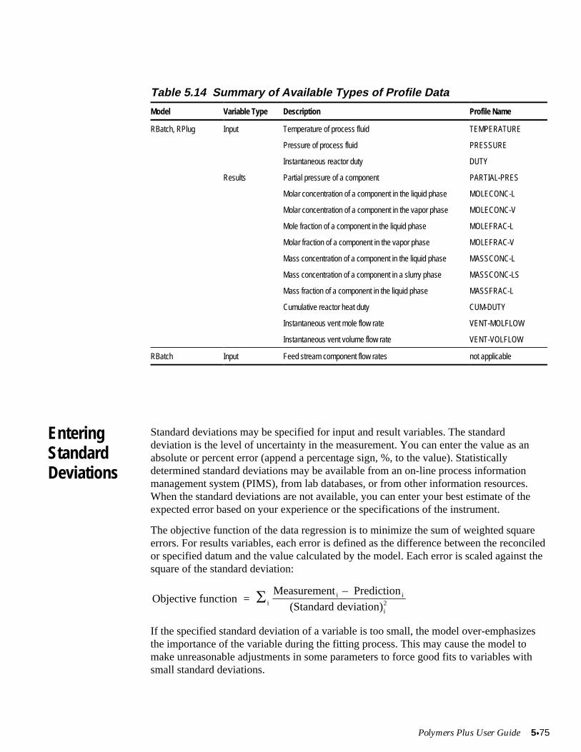
Polymers Plus User Guide 5x75
Table 5.14 Summary of Available Types of Profile Data
Model Variable Type Description Profile Name
RBatch, RPlug Input Temperature of process fluid TEMPERATURE
Pressure of process fluid PRESSURE
Instantaneous reactor duty DUTY
Results Partial pressure of a component PARTIAL-PRES
Molar concentration of a component in the liquid phase MOLECONC-L
Molar concentration of a component in the vapor phase MOLECONC-V
Mole fraction of a component in the liquid phase MOLEFRAC-L
Molar fraction of a component in the vapor phase MOLEFRAC-V
Mass concentration of a component in the liquid phase MASSCONC-L
Mass concentration of a component in a slurry phase MASSCONC-LS
Mass fraction of a component in the liquid phase MASSFRAC-L
Cumulative reactor heat duty CUM-DUTY
Instantaneous vent mole flow rate VENT-MOLFLOW
Instantaneous vent volume flow rate VENT-VOLFLOW
RBatch Input Feed stream component flow rates not applicable
EnteringStandardDeviations
Standard deviations may be specified for input and result variables. The standarddeviation is the level of uncertainty in the measurement. You can enter the value as anabsolute or percent error (append a percentage sign, %, to the value). Statisticallydetermined standard deviations may be available from an on-line process informationmanagement system (PIMS), from lab databases, or from other information resources.When the standard deviations are not available, you can enter your best estimate of theexpected error based on your experience or the specifications of the instrument.
The objective function of the data regression is to minimize the sum of weighted squareerrors. For results variables, each error is defined as the difference between the reconciledor specified datum and the value calculated by the model. Each error is scaled against thesquare of the standard deviation:
Objective function = Measurement Prediction
(Standard deviation)ii i
i26
�
If the specified standard deviation of a variable is too small, the model over-emphasizesthe importance of the variable during the fitting process. This may cause the model tomake unreasonable adjustments in some parameters to force good fits to variables withsmall standard deviations.
STEADY-STATE MODELS Data Fitting
5x76
You must be careful to consider both the precision and accuracy of each variable. Forexample, a variable may have a low standard deviation because it is very precise (itreproduces well in successive trials), but the measurement may be inaccurate (it may notreflect the true value of the measured parameter). Consider the case where a levelcontroller may show little deviation in the liquid volume in a reactor, but the calibrationof the level transducer may not be accurate to within ten percent of the real liquid volume.In this case, the standard deviation of the specified liquid volume should be large enoughto reflect the accuracy of the volume, not the deviation of the liquid level.
If standard deviations are specified for input variables, the model reconciles thesevariables. If you do not specify the standard deviation of an input variable, the modelassumes the specified values are exact. Reconciling input variables accounts formeasurement errors in the operating conditions and can lead to better models, but it cansubstantially increase how long the run takes to complete.
Standard deviations must be specified for each of the result variables. Specify reasonablestandard deviations to keep the model from forcing a match by making wild adjustmentsto the parameters. The specified standard deviations are probably too small (or the dataquality is poor) if several of the parameters reach their upper or lower bounds.
Defining DataRegressionCases
You can fit any number of data sets in the same regression case. Point-Data and Profile-Data may both be included. Each regression case must involve at least one estimatedparameter and at least one reconciled input variable. There are no upper limits to thenumber of estimated parameters and reconciled inputs, however the required simulationtime is very sensitive to the number of variables included in each regression case.
Each input variable with a non-zero standard deviation is reconciled (adjusted). Thereconciled inputs are tabulated in the regression results.
Each estimated parameter must be defined in the base case, or have a default value (suchas a physical property parameter). The specified values for the base case run are used asthe initial guesses for the regression. If the base-case value lies outside the specifiedbounds, the boundary condition closest to the base case value is used.
Polymers Plus User Guide 5x77
SequencingDataRegressionCases
For data fit problems, Aspen Plus will:
x Run the base-case simulationx Execute the data regressionx Replace the base-case parameter values with the estimated parameter values and rerun
the base-case simulation
If Case-Study or Sensitivity blocks are present, Aspen Plus runs them after the regressionis complete. The estimated parameter values are used to calculate the results for theseblocks.
Flowsheet convergence loops and Design-Specification loops are used in the preliminaryand final base-case simulations and they are sequenced inside the data regression loop.The sequencing of Fortran blocks and Transfer blocks depends on which variables areaccessed.
If more than one regression is included in a simulation, the regressions can be affectedsequentially. Each successive regression uses the estimated parameters from the previousregression.
Regression blocks can be manually sequenced if the automatic sequence does not meetthe needs of a particular run, however automatic sequencing is usually the best choice.
STEADY-STATE MODELS Data Fitting
5x78
InterpretingDataRegressionResults
The key results of the data regression tool are:x The Chi-square statistic and critical Chi-square value for the fit.x Estimates and standard deviations for each estimated parameter.x A table of the measured values, estimated values, and normalized residuals for each
data set.
The Chi-square value is an indicator of the quality of the fit. A model is considered wellfit if the Chi-square value falls below the critical Chi-square value. The reliability ofdifferent fits or different modeling approaches can be tested by comparing the Chi-squarevalues of the fits. For example, suppose a reactor is thought to have non-ideal mixing.This assumption can be evaluated by developing two models, one which assumes idealmixing (one CSTR stage) and one which assumes non-ideal mixing (a series of CSTRstages). The two models can be fit against the same data using the same parameters. Themodel with the lower Chi-square statistic represents the data more accurately, and can beconsidered the most realistic
x
Ideally, the standard deviations of the estimated parameters are small, and the confidenceinterval of each parameter is narrow. In practice, however, the standard deviation of theparameters may be relatively large. This does not necessarily indicate a poor fit. Forexample, if the activation energy and pre-exponential factor for a reaction are bothincluded as estimated parameters in the data regression, then the standard deviation of theestimated pre-exponential factor will be large. In this example, small differences in oneparameter (the activation energy) requires large differences in another parameter (the pre-exponential factor) to keep the model predictions relatively constant.
The residual values are indicative of the difference between the measured data and modelpredictions. For fitted data, the residuals are defined as:
Residual = (Measured value - Predicted value ) (Standard deviationi i i2
i/ )
For reconciled data, the residuals are defined as:
Residual = (Measured value - Estimated value ) (Standard deviationi i i2
i/ )
Review the residual values to verify they are sensible. Large residual values may indicatea major problem with the model or data, or may reflect an unreasonably tight standarddeviation. Never specify extremely tight standard deviations. This causes the dataregression algorithm to waste time attempting to obtain tight fits on some variables. Ifsome data are considered extremely accurate, they should be assigned standard deviationsof zero.
The regression results may be plotted against the initial estimates and measured data.Plots of this type include a 45q dotted line which indicates a “perfect fit”, e.g., eachprediction is exactly equal to the measured data. Points which fall far from this line arethe least well fit. Verify these outliers to make sure the data is correctly entered into themodel and that the units of measurement are consistent.
Polymers Plus User Guide 5x79
TroubleshootingConvergenceProblems
If the data regression tool fails to converge, check the objective function. A largeobjective function value indicates a poor fit between the model predictions and measureddata. If the objective function is large, review the residual values for each type ofmeasured data. Large residual values may indicate a very basic error in the data entry. Forexample, the data may be entered in the wrong units or there may be typing errors in thespecified values. Always review the model thoroughly to eliminate these types ofproblems before adjusting convergence parameters or making other major changes to theregression.
Convergence errors can occur for a number of reasons. When a problem occurs, ask:
x Does the base case model converge well and give reasonable results?x Is the base case model formulated to handle data which may be out of mass or energy
balance?x Are the initial estimates of the parameters good enough?x Are the specified standard deviations reasonable?x Do the model inputs completely determine the measured results?x Do the specified bounds allow the regression to take the model into infeasible regions,
causing the unit operation blocks or flowsheet convergence to fail?x Are the assumptions and simplifications in the model reasonable?
Regression runs with many variables and runs for highly non-linear models may still bedifficult to converge. In some cases, the convergence criteria may be unnecessarily tight.Table 5.15 summarizes several convergence parameters which can be used to tune aregression run. It is not necessary to adjust the convergence parameters for mostregressions.
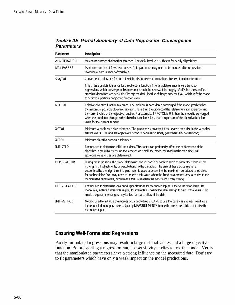
STEADY-STATE MODELS Data Fitting
5x80
Table 5.15 Partial Summary of Data Regression ConvergenceParameters
Parameter Description
ALG-ITERATION Maximum number of algorithm iterations. The default value is sufficient for nearly all problems
MAX-PASSES Maximum number of flowsheet passes. This parameter may need to be increased for regressionsinvolving a large number of variables.
SSQTOL Convergence tolerance for sum of weighted square errors (Absolute objective function tolerance)
This is the absolute tolerance for the objective function. The default tolerance is very tight, soregressions which converge to this tolerance should be reviewed thoroughly. Verify that the specifiedstandard deviations are sensible. Change the default value of this parameter if you which to fit the modelto achieve a particular objective function value.
RFCTOL Relative objective function tolerance. The problem is considered converged if the model predicts thatthe maximum possible objective function is less than the product of the relative function tolerance andthe current value of the objective function. For example, if RFCTOL is 0.1, then the model is convergedwhen the predicted change in the objective function is less than ten percent of the objective functionvalue for the current iteration.
XCTOL Minimum variable step-size tolerance. The problem is converged if the relative step size in the variablesfalls below XCTOL and the objective function is decreasing slowly (less than 50% per iteration).
XFTOL Minimum objective step-size tolerance
INIT-STEP Factor used to determine initial step sizes. This factor can profoundly affect the performance of thealgorithm. If the initial steps are too large or too small, the model must adjust the step size untilappropriate step sizes are determined.
PERT-FACTOR During the regression, the model determines the response of each variable to each other variable bymaking small adjustments, or pertubations, to the variables. The size of these adjustments isdetermined by the algorithm, this parameter is used to determine the maximum pertubation step sizesfor each variable. You may need to increase this value when the fitted data are not very sensitive to themanipulated parameters, or decrease this value when the sensitivity is very strong.
BOUND-FACTOR Factor used to determine lower and upper bounds for reconciled inputs. If the value is too large, themodel may enter an infeasible region, for example a stream flow rate may go to zero. If the value is toosmall, the parameter ranges may be too narrow to allow fit the data.
INIT-METHOD Method used to initialize the regression. Specify BASE-CASE to use the base case values to initializethe reconciled input parameters. Specify MEASUREMENTS to use the measured data to initialize thereconciled inputs.
Ensuring Well-Formulated Regressions
Poorly formulated regressions may result in large residual values and a large objectivefunction. Before starting a regression run, use sensitivity studies to test the model. Verifythat the manipulated parameters have a strong influence on the measured data. Don’t tryto fit parameters which have only a weak impact on the model predictions.
Polymers Plus User Guide 5x81
Make sure the parameter ranges are sensible. It is a waste of time to fit a parameter withina narrow range (less than 5%). On the other hand, if the range is too large, the regressionalgorithm may push the model into an infeasible region. For example, if the distillate tofeed ratio in a column is allowed to decrease to zero, the column model will fail.
The way the data regression is formulated has a major influence on how quickly andeasily the problem converges. De-couple the manipulated variables as much as possible.For example, don’t fit the rate constants and phase equilibrium parameters at the sametime if the two sets of parameters can be fit independently in two smaller data regressionruns.
Use the weighing factors if some sets of data are more reliable than others. A largerweight may be assigned to a set of data that are based on long-term averages from theprocess information management system, lower weights might be assigned to data basedon poorly kept records from the distant past.
Make sure the manipulated parameters can be determined from the available data. Forexample, the activation energy of a reaction cannot be determined from isothermal data.
The base-case file needs to be formulated in a robust manner. If the base case model doesnot converge reliably away from the base case condition, then it is likely that theregression run will fail. Use the sensitivity tool to verify that the model is stable over theentire range of each manipulated parameter and to verify that the model is sensitive toeach parameter.
Where possible, use relative or normalized inputs instead of absolute inputs. For example,in column models use the distillate to feed ratio (D:F) instead of distillate flow rate. Usepressure drop specifications instead of pressure. These specifications make the modelmore reliable and help to avoid problems which occur if the measured data is out of massbalance with each other.
Fitting Activation Energy
It is tempting to try to fit activation energies and pre-exponential factors in the sameregression run. This can lead to significant headaches if the problem is not approachedright. Consider, for example, the standard Arrehnius rate expression:
k knet o
E
RTact
�
exp
Using this expression, the net rate constant, knet , is sensitive to the activation energy,Eact . If the activation energy is adjusted a little bit, a large adjustment must be made tothe pre-exponential factor to offset this difference. In other words, the activation energycontrols the magnitude of the reaction rate as well as the temperature sensitivity of thereaction rate.
STEADY-STATE MODELS Data Fitting
5x82
A better approach is to use the modified Arrehnius expression:
k knet o
E
R T Tact
ref
��
§
©¨̈
·
¹¸̧
exp
1 1
The parameter Tref is a reference temperature which typically represents the middle of the
temperature range used to estimate the activation energy. Using this formula, the net rateconstant, knet , remains constant at the reference temperature regardless of the value of theactivation energy. With this approach, the pre-exponential factor, ko , controls themagnitude of the reaction rate at the reference temperature. The activation energy, Eact ,controls the temperature sensitivity of the rate constant. This makes it much easier to fitthe model.
Scaling the Fitted Parameters
When several types of parameters are adjusted in the same run, the magnitude of themanipulated parameters may influence how well the data regression converges. Ideally,the manipulated parameters should be within several orders of magnitude of each other.
Suppose, for example, the manipulated parameters include rate constants for severaldifferent types of reactions. These expected values of the rate constants may differ byseveral orders of magnitude. In this situation, the regression procedure may over-emphasize the manipulated variables with the smallest magnitude.
You can get around this problem using two Fortran blocks as shown in Example 3. Useone Fortran block to define a PARAMETER variable for each manipulated variable in theregression. Initialize each parameter to one. Use a second Fortran block to READ theseparameter values, to multiply them by base case values, and then WRITE the results to themanipulated variables. In the data regression block, manipulate the PARAMETERvariables.
This technique allows the data regression to operate on normalized variables instead ofabsolute variables which makes it much easier for the regression algorithm to chooseappropriate step sizes and ensures that the variables are given equal weighting by thealgorithm.
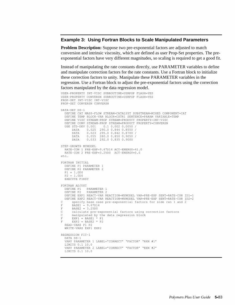
Polymers Plus User Guide 5x83
Example 3: Using Fortran Blocks to Scale Manipulated Parameters
Problem Description: Suppose two pre-exponential factors are adjusted to matchconversion and intrinsic viscosity, which are defined as user Prop-Set properties. The pre-exponential factors have very different magnitudes, so scaling is required to get a good fit.
Instead of manipulating the rate constants directly, use PARAMETER variables to defineand manipulate correction factors for the rate constants. Use a Fortran block to initializethese correction factors to unity. Manipulate these PARAMETER variables in theregression. Use a Fortran block to adjust the pre-exponential factors using the correctionfactors manipulated by the data regression model.USER-PROPERTY INT-VISC SUBROUTINE=USRPSP FLASH=YESUSER-PROPERTY CONVERSN SUBROUTINE=USRPSP FLASH=YESPROP-SET INT-VISC INT-VISCPROP-SET CONVERSN CONVERSN
DATA-SET DS-1 DEFINE CAT MASS-FLOW STREAM=CATALYST SUBSTREAM=MIXED COMPONENT=CAT DEFINE TEMP BLOCK-VAR BLOCK=CSTR1 SENTENCE=PARAM VARIABLE=TEMP DEFINE VISC STREAM-PROP STREAM=PRODUCT PROPERTY=INT-VISC DEFINE CONV STREAM-PROP STREAM=PRODUCT PROPERTY=CONVERSN USE STD-DEV 0.001 0.1 0.002 0.0050 / DATA 0.025 290.0 0.844 0.8550 / DATA 0.023 295.0 0.842 0.8700 / DATA 0.055 280.0 0.850 0.9050 / DATA 0.033 292.0 0.835 0.9000
STEP-GROWTH MYMODEL RATE-CON 1 PRE-EXP=9.67D14 ACT-ENERGY=41.0 RATE-CON 2 PRE-EXP=3.25D0 ACT-ENERGY=0.0etc…
FORTRAN INITIAL DEFINE P1 PARAMETER 1 DEFINE P2 PARAMETER 2 P1 = 1.0D0 P2 = 1.0D0 EXECUTE FIRST
FORTRAN ADJUST DEFINE P1 PARAMETER 1 DEFINE P2 PARAMETER 2 DEFINE EXP1 REACT-VAR REACTION=MYMODEL VAR=PRE-EXP SENT=RATE-CON ID1=1 DEFINE EXP2 REACT-VAR REACTION=MYMODEL VAR=PRE-EXP SENT=RATE-CON ID2=2C specify base case pre-exponential factors for side rxn 1 and 2F BASE1 = 9.67D14F BASE2 = 3.25D0C calculate pre-exponential factors using correction factorsC manipulated by the data regression blockF EXP1 = BASE1 * P1F EXP2 = BASE2 * P2 READ-VARS P1 P2 WRITE-VARS EXP1 EXP2
REGRESSION FIT-1 DATA DS-1 VARY PARAMETER 1 LABEL=”CORRECT” “FACTOR” “RXN #1” LIMITS 0.1 10.0 VARY PARAMETER 2 LABEL=”CORRECT” “FACTOR” “RXN #2” LIMITS 0.1 10.0

STEADY-STATE MODELS Data Fitting
5x84
Polymers Plus User Guide 5x85
5.3 USER MODELS
This section discusses the features available in Polymers Plus for incorporating usermodules into a simulation model.
Topics covered include:
x User Unit Operation Modelsx User Kinetic Modelsx User Physical Property Models
More details concerning User Models are available in Aspen Plus User Models.
USER UNIT OPERATION MODELS
There are cases where users may need to create special models to represent a process.Usually these models can be configured by combining several of the standard unit operationbuilding blocks. For more complex reactor geometries or in order to represent highly non-ideal systems users may need to provide their own model as a Fortran subroutine.
There are two user unit operation blocks available: USER and USER2. The first allows alimited number of inlet and outlet streams. The second allows multiple inlet and outletstreams. Both unit operations take full advantage of the Aspen Plus flowsheetingcapabilities. The required Fortran subroutine must process the feed streams and return thecondition and composition of the outlet streams.
5.3
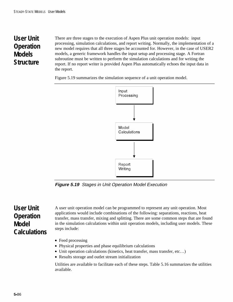
STEADY-STATE MODELS User Models
5x86
User UnitOperationModelsStructure
There are three stages to the execution of Aspen Plus unit operation models: inputprocessing, simulation calculations, and report writing. Normally, the implementation of anew model requires that all three stages be accounted for. However, in the case of USER2models, a generic framework handles the input setup and processing stage. A Fortransubroutine must be written to perform the simulation calculations and for writing thereport. If no report writer is provided Aspen Plus automatically echoes the input data inthe report.
Figure 5.19 summarizes the simulation sequence of a unit operation model.
Figure 5.19 Stages in Unit Operation Model Execution
User UnitOperationModelCalculations
A user unit operation model can be programmed to represent any unit operation. Mostapplications would include combinations of the following: separations, reactions, heattransfer, mass transfer, mixing and splitting. There are some common steps that are foundin the simulation calculations within unit operation models, including user models. Thesesteps include:
x Feed processingx Physical properties and phase equilibrium calculationsx Unit operation calculations (kinetics, heat transfer, mass transfer, etc…)x Results storage and outlet stream initialization
Utilities are available to facilitate each of these steps. Table 5.16 summarizes the utilitiesavailable.
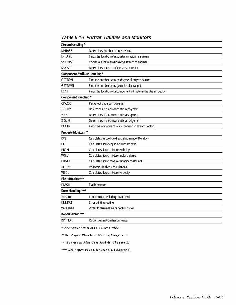
Polymers Plus User Guide 5x87
Table 5.16 Fortran Utilities and MonitorsStream Handling *
NPHASE Determines number of substreams
LPHASE Finds the location of a substream within a stream
SSCOPY Copies a substream from one stream to another
NSVAR Determines the size of the stream vector
Component Attribute Handling *
GETDPN Find the number average degree of polymerization
GETMWN Find the number average molecular weight
LCATT Finds the location of a component attribute in the stream vector
Component Handling *
CPACK Packs out trace components
ISPOLY Determines if a component is a polymer
ISSEG Determines if a component is a segment
ISOLIG Determines if a component is an oligomer
KCCID Finds the component index (position in stream vector)
Property Monitors **
KVL Calculates vapor-liquid equilibrium ratio (K-value)
KLL Calculates liquid-liquid equilibrium ratio
ENTHL Calculates liquid mixture enthalpy
VOLV Calculates liquid mixture molar volume
FUGLY Calculates liquid mixture fugacity coefficient
IDLGAS Performs ideal gas calculations
VISCL Calculates liquid mixture viscosity
Flash Routine ***
FLASH Flash monitor
Error Handling ****
IRRCHK Function to check diagnostic level
ERRPRT Error printing routine
WRTTRM Writer to terminal file or control panel
Report Writer ****
RPTHDR Report pagination /header writer
* See Appendix H of this User Guide.
** See Aspen Plus User Models, Chapter 3.
*** See Aspen Plus User Models, Chapter 2.
**** See Aspen Plus User Models, Chapter 4.
STEADY-STATE MODELS User Models
5x88
Stream Processing
In order to perform its calculations the user model must be able to read and process theAspen Plus stream structure. The stream structure is documented in Appendix C of AspenPlus User Models. Example 1 shows a USER2 model routine.
Note that data in the streams coming in and out of the model are stored in SIunits.
There are several utilities available for stream processing. These perform functions suchas finding the number of stream variables, i.e. the size of the stream vector, copying onestream to another, finding the total number of substreams, and finding specific substreamswithin a stream. Several stream handling utilities are documented in Appendix H: FortranUtilities of this User Guide.
In addition to the standard composition and state information found in the streamstructure, there are also component attributes. If the user model processes polymers, thencomponent attributes must be processed and their outlet stream values must be calculatedand stored. The attributes available include polymer properties such as degree ofpolymerization, molecular weight, polydispersity, and copolymer composition. These aredocumented in Section 2.2 of this User Guide. In order to process attributes, there areFortran utilities available that perform functions such as copying attributes from onestream to another, retrieving number average molecular weight and degree ofpolymerization, retrieving copolymer composition, locating specific component attributeswithin the stream vector, and determining the size of a vector component attribute. Thecomponent attribute handling utilities are documented in Appendix H.
There are also utilities for processing components: for excluding trace components, fordetermining component type (polymer, oligomer, segment, catalyst), etc. These can befound with the component attribute processing utilities.
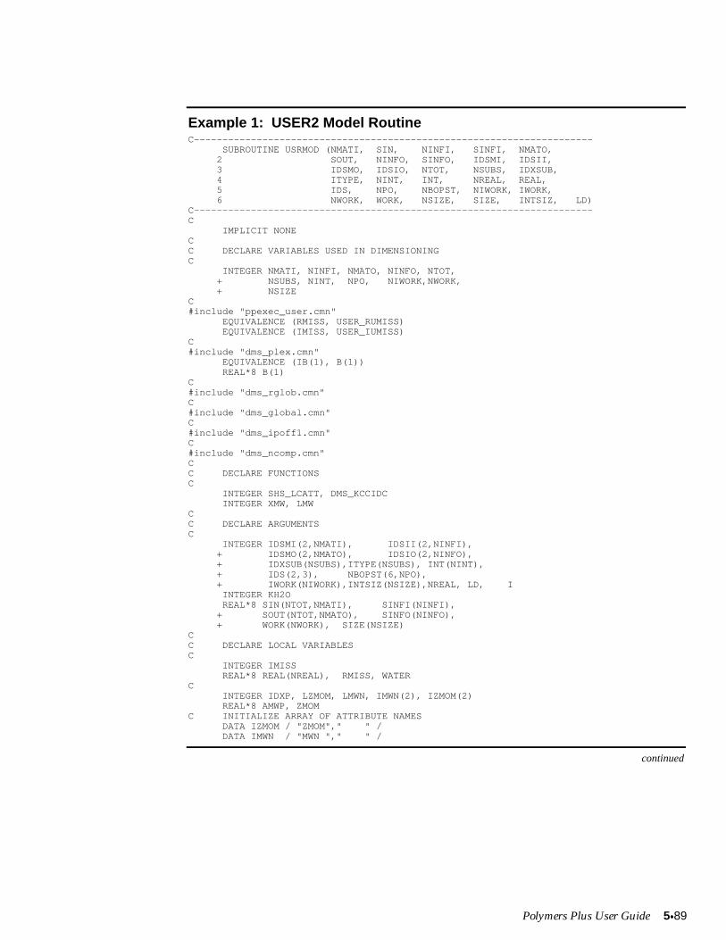
Polymers Plus User Guide 5x89
Example 1: USER2 Model RoutineC---------------------------------------------------------------------- SUBROUTINE USRMOD (NMATI, SIN, NINFI, SINFI, NMATO, 2 SOUT, NINFO, SINFO, IDSMI, IDSII, 3 IDSMO, IDSIO, NTOT, NSUBS, IDXSUB, 4 ITYPE, NINT, INT, NREAL, REAL, 5 IDS, NPO, NBOPST, NIWORK, IWORK, 6 NWORK, WORK, NSIZE, SIZE, INTSIZ, LD)C----------------------------------------------------------------------C IMPLICIT NONECC DECLARE VARIABLES USED IN DIMENSIONINGC INTEGER NMATI, NINFI, NMATO, NINFO, NTOT, + NSUBS, NINT, NPO, NIWORK,NWORK, + NSIZEC#include "ppexec_user.cmn" EQUIVALENCE (RMISS, USER_RUMISS) EQUIVALENCE (IMISS, USER_IUMISS)C#include "dms_plex.cmn" EQUIVALENCE (IB(1), B(1)) REAL*8 B(1)C#include "dms_rglob.cmn"C#include "dms_global.cmn"C#include "dms_ipoff1.cmn"C#include "dms_ncomp.cmn"CC DECLARE FUNCTIONSC INTEGER SHS_LCATT, DMS_KCCIDC INTEGER XMW, LMWCC DECLARE ARGUMENTSC INTEGER IDSMI(2,NMATI), IDSII(2,NINFI), + IDSMO(2,NMATO), IDSIO(2,NINFO), + IDXSUB(NSUBS),ITYPE(NSUBS), INT(NINT), + IDS(2,3), NBOPST(6,NPO), + IWORK(NIWORK),INTSIZ(NSIZE),NREAL, LD, I INTEGER KH2O REAL*8 SIN(NTOT,NMATI), SINFI(NINFI), + SOUT(NTOT,NMATO), SINFO(NINFO), + WORK(NWORK), SIZE(NSIZE)CC DECLARE LOCAL VARIABLESC INTEGER IMISS REAL*8 REAL(NREAL), RMISS, WATERC INTEGER IDXP, LZMOM, LMWN, IMWN(2), IZMOM(2) REAL*8 AMWP, ZMOMC INITIALIZE ARRAY OF ATTRIBUTE NAMES DATA IZMOM / "ZMOM"," " / DATA IMWN / "MWN "," " /
continued
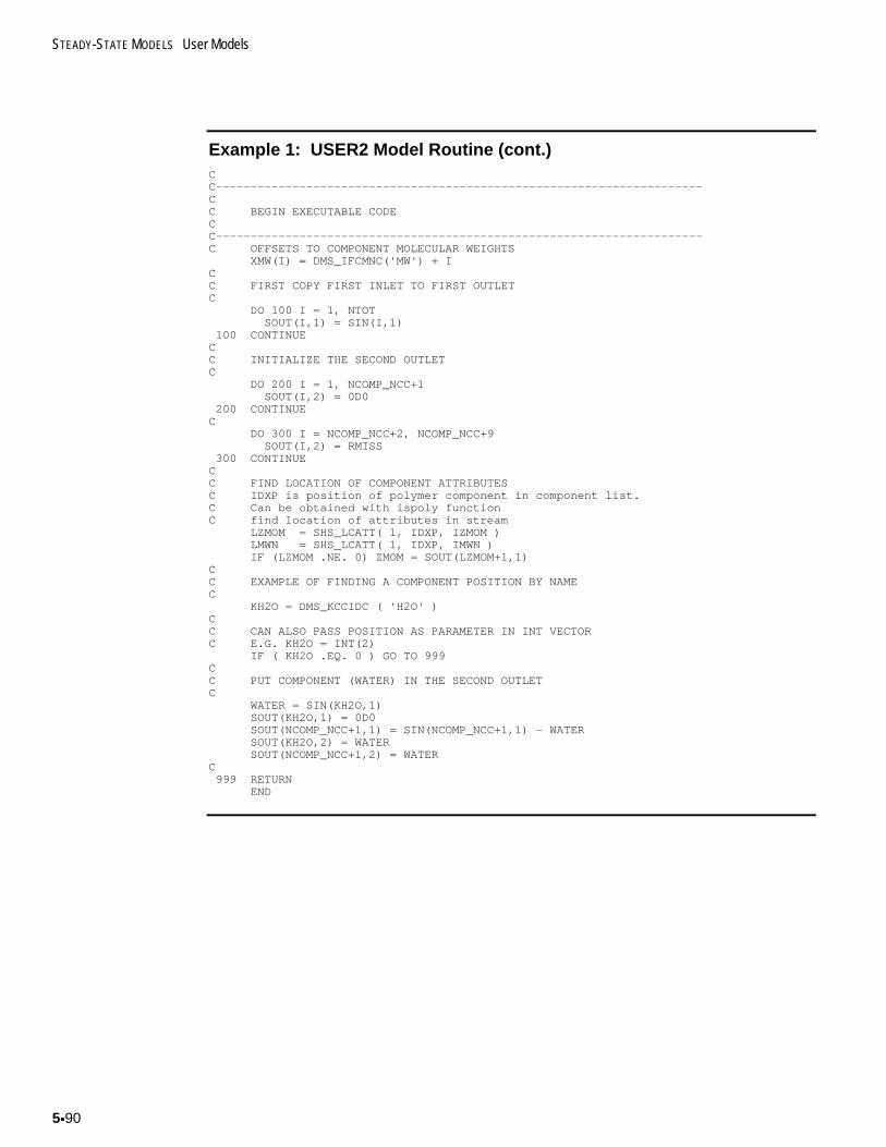
STEADY-STATE MODELS User Models
5x90
Example 1: USER2 Model Routine (cont.)CC----------------------------------------------------------------------CC BEGIN EXECUTABLE CODECC----------------------------------------------------------------------C OFFSETS TO COMPONENT MOLECULAR WEIGHTS XMW(I) = DMS_IFCMNC('MW') + ICC FIRST COPY FIRST INLET TO FIRST OUTLETC DO 100 I = 1, NTOT SOUT(I,1) = SIN(I,1) 100 CONTINUECC INITIALIZE THE SECOND OUTLETC DO 200 I = 1, NCOMP_NCC+1 SOUT(I,2) = 0D0 200 CONTINUEC DO 300 I = NCOMP_NCC+2, NCOMP_NCC+9 SOUT(I,2) = RMISS 300 CONTINUECC FIND LOCATION OF COMPONENT ATTRIBUTESC IDXP is position of polymer component in component list.C Can be obtained with ispoly functionC find location of attributes in stream LZMOM = SHS_LCATT( 1, IDXP, IZMOM ) LMWN = SHS_LCATT( 1, IDXP, IMWN ) IF (LZMOM .NE. 0) ZMOM = SOUT(LZMOM+1,1)CC EXAMPLE OF FINDING A COMPONENT POSITION BY NAMEC KH2O = DMS_KCCIDC ( 'H2O' )CC CAN ALSO PASS POSITION AS PARAMETER IN INT VECTORC E.G. KH2O = INT(2) IF ( KH2O .EQ. 0 ) GO TO 999CC PUT COMPONENT (WATER) IN THE SECOND OUTLETC WATER = SIN(KH2O,1) SOUT(KH2O,1) = 0D0 SOUT(NCOMP_NCC+1,1) = SIN(NCOMP_NCC+1,1) - WATER SOUT(KH2O,2) = WATER SOUT(NCOMP_NCC+1,2) = WATERC 999 RETURN END
Polymers Plus User Guide 5x91
Physical Property Calculations
Physical properties and phase equilibrium calculations can be performed within a usermodel. Property methods, models, and parameters specified in the input either through abuilt-in or a user-defined property method, can be used for the user model calculations.This can be done through property monitors. The user model requests the property ofinterest by calling a specific monitor, sets the state information and calculation codes inthe call to the monitors, and in turn obtains thermodynamic properties such as fugacitycoefficients, enthalpies, entropies, molar volumes, etc. A flash calculation routine is alsoavailable. See Table 5.16 for a listing of frequently used property monitors. The FLASHroutine and the property monitors are documented in Chapters 2 and 3 of Aspen Plus UserModels. See also User Physical Property Models later in this section.
Unit Operation Calculations
The purpose of a user unit operation block is to allow the flexibility to program usercorrelations or algorithms to represent a process. Independently from the physicalproperty calculations for which monitors are provided, users can take advantage of theFortran subroutine structure to incorporate the calculations needed to represent theirprocess. Aspen Plus System Management documents programming guidelines to befollowed when defining the model calculations. The calculations performed within a userunit operator model for a polymer system are similar to those that could be performedwithin a kinetic model. See User Kinetic Models later in this section.
Diagnostics
Throughout the simulation calculations, a user model may call the Aspen Plus errorhandler to issue diagnostic messages ranging from fatal errors to warnings andinformation. The error handler is documented in Chapter 4 of Aspen Plus User Models.These diagnostics can be written to the terminal or the control panel. The USER labeledcommons contains output file numbers through which the terminal, control panel andsimulation files can be accessed. See Appendix A of Aspen Plus User Models for adescription of the USER labeled common.
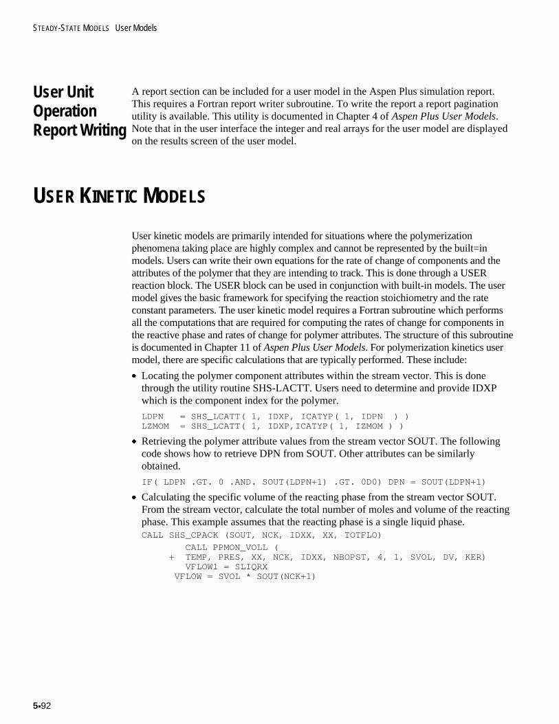
STEADY-STATE MODELS User Models
5x92
User UnitOperationReport Writing
A report section can be included for a user model in the Aspen Plus simulation report.This requires a Fortran report writer subroutine. To write the report a report paginationutility is available. This utility is documented in Chapter 4 of Aspen Plus User Models.Note that in the user interface the integer and real arrays for the user model are displayedon the results screen of the user model.
USER KINETIC MODELS
User kinetic models are primarily intended for situations where the polymerizationphenomena taking place are highly complex and cannot be represented by the built=inmodels. Users can write their own equations for the rate of change of components and theattributes of the polymer that they are intending to track. This is done through a USERreaction block. The USER block can be used in conjunction with built-in models. The usermodel gives the basic framework for specifying the reaction stoichiometry and the rateconstant parameters. The user kinetic model requires a Fortran subroutine which performsall the computations that are required for computing the rates of change for components inthe reactive phase and rates of change for polymer attributes. The structure of this subroutineis documented in Chapter 11 of Aspen Plus User Models. For polymerization kinetics usermodel, there are specific calculations that are typically performed. These include:
x Locating the polymer component attributes within the stream vector. This is donethrough the utility routine SHS-LACTT. Users need to determine and provide IDXPwhich is the component index for the polymer.
LDPN = SHS_LCATT( 1, IDXP, ICATYP( 1, IDPN ) )LZMOM = SHS_LCATT( 1, IDXP,ICATYP( 1, IZMOM ) )
x Retrieving the polymer attribute values from the stream vector SOUT. The followingcode shows how to retrieve DPN from SOUT. Other attributes can be similarlyobtained.
IF( LDPN .GT. 0 .AND. SOUT(LDPN+1) .GT. 0D0) DPN = SOUT(LDPN+1)
x Calculating the specific volume of the reacting phase from the stream vector SOUT.From the stream vector, calculate the total number of moles and volume of the reactingphase. This example assumes that the reacting phase is a single liquid phase.CALL SHS_CPACK (SOUT, NCK, IDXX, XX, TOTFLO)
CALL PPMON_VOLL ( + TEMP, PRES, XX, NCK, IDXX, NBOPST, 4, 1, SVOL, DV, KER) VFLOW1 = SLIQRX VFLOW = SVOL * SOUT(NCK+1)
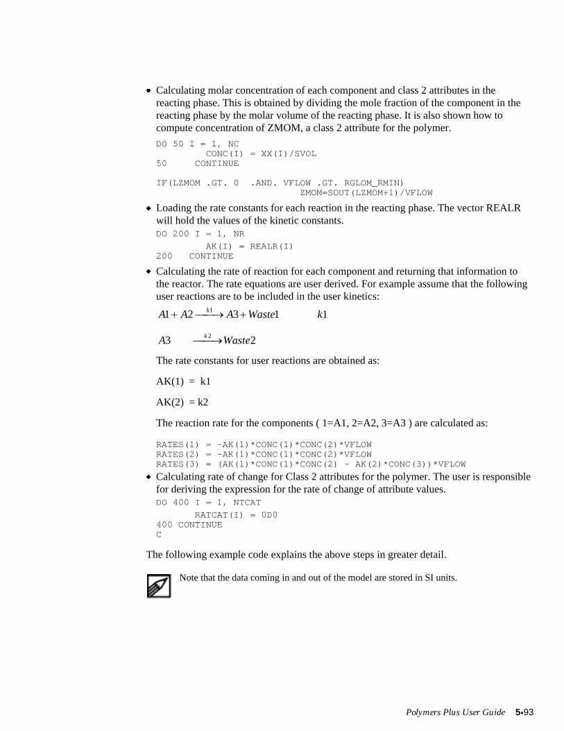
Polymers Plus User Guide 5x93
x Calculating molar concentration of each component and class 2 attributes in thereacting phase. This is obtained by dividing the mole fraction of the component in thereacting phase by the molar volume of the reacting phase. It is also shown how tocompute concentration of ZMOM, a class 2 attribute for the polymer.
DO 50 I = 1, NC CONC(I) = XX(I)/SVOL50 CONTINUE
IF(LZMOM .GT. 0 .AND. VFLOW .GT. RGLOM_RMIN) ZMOM=SOUT(LZMOM+1)/VFLOW
x Loading the rate constants for each reaction in the reacting phase. The vector REALRwill hold the values of the kinetic constants.DO 200 I = 1, NR
AK(I) = REALR(I)200 CONTINUE
x Calculating the rate of reaction for each component and returning that information tothe reactor. The rate equations are user derived. For example assume that the followinguser reactions are to be included in the user kinetics:
A A A Waste kk1 2 3 1 11� � o� �
A Wastek3 22� o�
The rate constants for user reactions are obtained as:
AK(1) = k1
AK(2) = k2
The reaction rate for the components ( 1=A1, 2=A2, 3=A3 ) are calculated as:
RATES(1) = -AK(1)*CONC(1)*CONC(2)*VFLOWRATES(2) = -AK(1)*CONC(1)*CONC(2)*VFLOWRATES(3) = (AK(1)*CONC(1)*CONC(2) - AK(2)*CONC(3))*VFLOW
x Calculating rate of change for Class 2 attributes for the polymer. The user is responsiblefor deriving the expression for the rate of change of attribute values.DO 400 I = 1, NTCAT
RATCAT(I) = 0D0400 CONTINUEC
The following example code explains the above steps in greater detail.
Note that the data coming in and out of the model are stored in SI units.
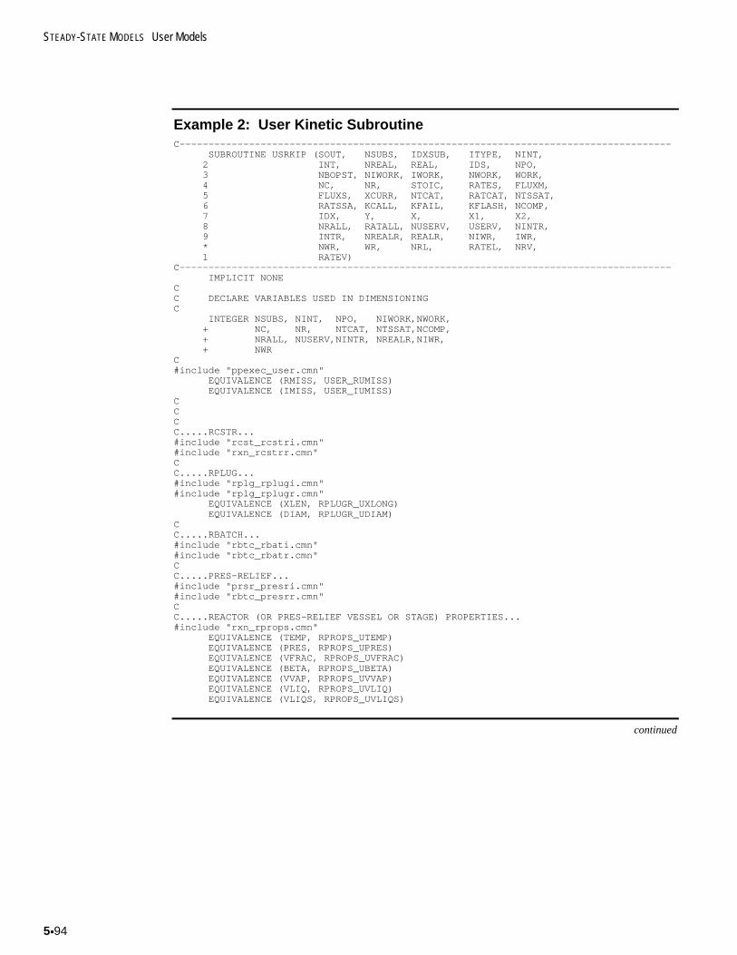
STEADY-STATE MODELS User Models
5x94
Example 2: User Kinetic SubroutineC------------------------------------------------------------------------------------- SUBROUTINE USRKIP (SOUT, NSUBS, IDXSUB, ITYPE, NINT, 2 INT, NREAL, REAL, IDS, NPO, 3 NBOPST, NIWORK, IWORK, NWORK, WORK, 4 NC, NR, STOIC, RATES, FLUXM, 5 FLUXS, XCURR, NTCAT, RATCAT, NTSSAT, 6 RATSSA, KCALL, KFAIL, KFLASH, NCOMP, 7 IDX, Y, X, X1, X2, 8 NRALL, RATALL, NUSERV, USERV, NINTR, 9 INTR, NREALR, REALR, NIWR, IWR, * NWR, WR, NRL, RATEL, NRV, 1 RATEV)C------------------------------------------------------------------------------------- IMPLICIT NONECC DECLARE VARIABLES USED IN DIMENSIONINGC INTEGER NSUBS, NINT, NPO, NIWORK,NWORK, + NC, NR, NTCAT, NTSSAT,NCOMP, + NRALL, NUSERV,NINTR, NREALR,NIWR, + NWRC#include "ppexec_user.cmn" EQUIVALENCE (RMISS, USER_RUMISS) EQUIVALENCE (IMISS, USER_IUMISS)CCCC.....RCSTR...#include "rcst_rcstri.cmn"#include "rxn_rcstrr.cmn"CC.....RPLUG...#include "rplg_rplugi.cmn"#include "rplg_rplugr.cmn" EQUIVALENCE (XLEN, RPLUGR_UXLONG) EQUIVALENCE (DIAM, RPLUGR_UDIAM)CC.....RBATCH...#include "rbtc_rbati.cmn"#include "rbtc_rbatr.cmn"CC.....PRES-RELIEF...#include "prsr_presri.cmn"#include "rbtc_presrr.cmn"CC.....REACTOR (OR PRES-RELIEF VESSEL OR STAGE) PROPERTIES...#include "rxn_rprops.cmn" EQUIVALENCE (TEMP, RPROPS_UTEMP) EQUIVALENCE (PRES, RPROPS_UPRES) EQUIVALENCE (VFRAC, RPROPS_UVFRAC) EQUIVALENCE (BETA, RPROPS_UBETA) EQUIVALENCE (VVAP, RPROPS_UVVAP) EQUIVALENCE (VLIQ, RPROPS_UVLIQ) EQUIVALENCE (VLIQS, RPROPS_UVLIQS)
continued
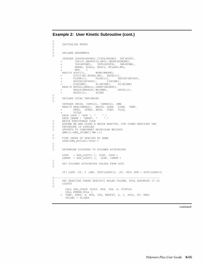
Polymers Plus User Guide 5x95
Example 2: User Kinetic Subroutine (cont.)
CC INITIALIZE RATESCCC DECLARE ARGUMENTSC INTEGER IDXSUB(NSUBS),ITYPE(NSUBS), INT(NINT), + IDS(2),NBOPST(6,NPO),IWORK(NIWORK), + IDX(NCOMP), INTR(NINTR), IWR(NIWR), + NREAL, KCALL, KFAIL, KFLASH,NRL, + NRV, I REAL*8 SOUT(1), WORK(NWORK), + STOIC(NC,NSUBS,NR), RATES(1), + FLUXM(1), FLUXS(1), RATCAT(NTCAT), + RATSSA(NTSSAT), Y(NCOMP), + X(NCOMP), X1(NCOMP), X2(NCOMP) REAL*8 RATALL(NRALL),USERV(NUSERV), + REALR(NREALR),WR(NWR), RATEL(1), + RATEV(1), XCURRCC DECLARE LOCAL VARIABLESC INTEGER IMISS, IDPN(2), IZMOM(2), XMW REAL*8 REAL(NREAL), RMISS, XLEN, DIAM, TEMP, + PRES, VFRAC, BETA, VVAP, VLIQ, + VLIQS DATA IDPN / "DPN ", " " / DATA IZMOM / "ZMOM", " " /C BEGIN EXECUTABLE CODEC ASSUME WE ARE USING A BATCH REACTOR. FOR OTHER REACTORS THEC PROCEDURE IS SIMILARC OFFSETS TO COMPONENT MOLECULAR WEIGHTS XMW(I)=DMS_IFCMNC('MW')+ICC FIND INDEX OF SPECIES BY NAME IDXP=DMS_KCCIDC('POLY')CCC DETERMINE POINTERS TO POLYMER ATTRIBUTES
LDPN = SHS_LCATT( 1, IDXP, IDPN ) LZMOM = SHS_LCATT( 1, IDXP, IZMOM )CC GET POLYMER ATTRIBUTES VALUES FROM SOUTC
IF( LDPN .GT. 0 .AND. SOUT(LDPN+1) .GT. 0D0) DPN = SOUT(LDPN+1)
C------------------------------------------------------------------C GET REACTING PHASE SPECIFIC MOLAR VOLUME, SVOL ASSUMING IT ISC LIQUIDC CALL SHS_CPACK (SOUT, NCK, IDX, X, TOTFLO) CALL PPMON_VOLL ( + TEMP, PRES, X, NCK, IDX, NBOPST, 4, 1, SVOL, DV, KER) VFLOW1 = SLIQRX
continued
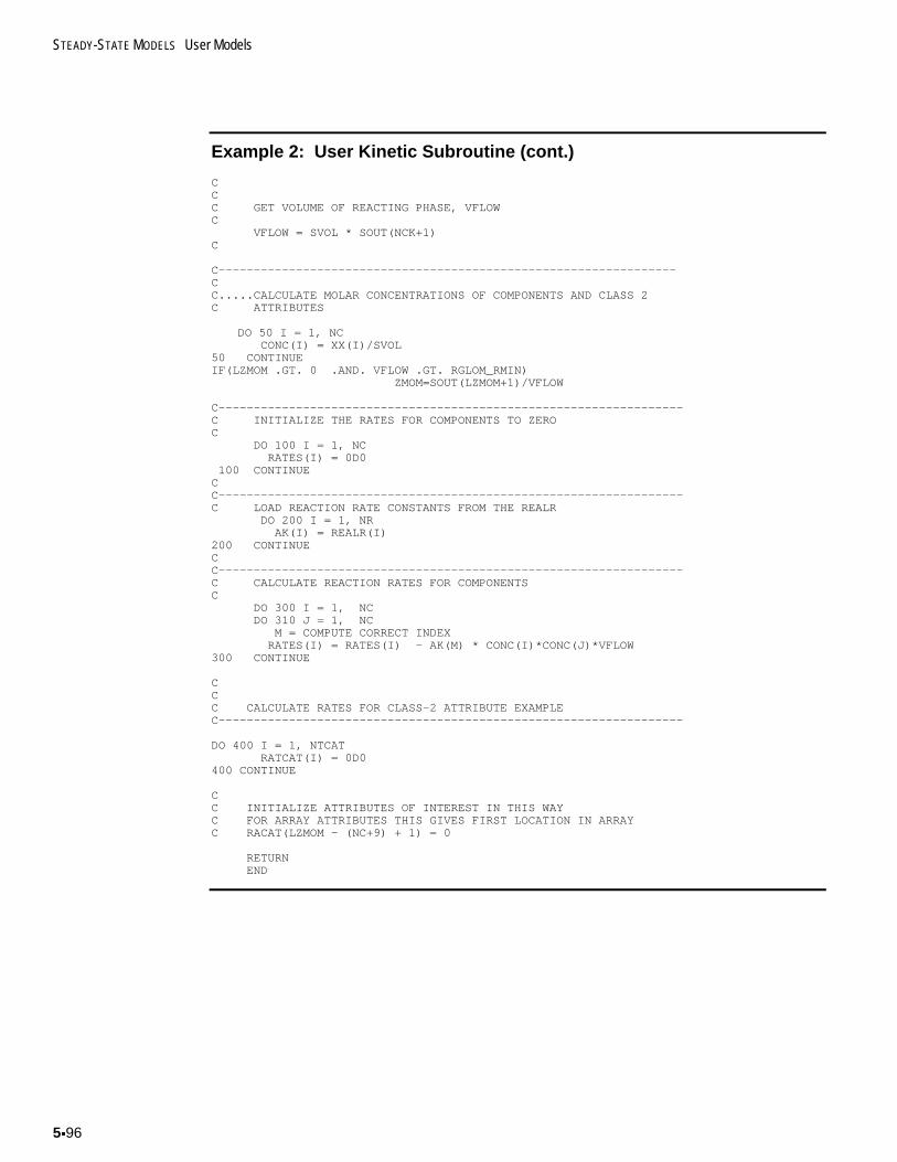
STEADY-STATE MODELS User Models
5x96
Example 2: User Kinetic Subroutine (cont.)
CCC GET VOLUME OF REACTING PHASE, VFLOWC VFLOW = SVOL * SOUT(NCK+1)C
C-----------------------------------------------------------------CC.....CALCULATE MOLAR CONCENTRATIONS OF COMPONENTS AND CLASS 2C ATTRIBUTES
DO 50 I = 1, NC CONC(I) = XX(I)/SVOL50 CONTINUEIF(LZMOM .GT. 0 .AND. VFLOW .GT. RGLOM_RMIN) ZMOM=SOUT(LZMOM+1)/VFLOW
C------------------------------------------------------------------C INITIALIZE THE RATES FOR COMPONENTS TO ZEROC DO 100 I = 1, NC RATES(I) = 0D0 100 CONTINUECC------------------------------------------------------------------C LOAD REACTION RATE CONSTANTS FROM THE REALR DO 200 I = 1, NR AK(I) = REALR(I)200 CONTINUECC------------------------------------------------------------------C CALCULATE REACTION RATES FOR COMPONENTSC DO 300 I = 1, NC DO 310 J = 1, NC M = COMPUTE CORRECT INDEX RATES(I) = RATES(I) - AK(M) * CONC(I)*CONC(J)*VFLOW300 CONTINUE
CCC CALCULATE RATES FOR CLASS-2 ATTRIBUTE EXAMPLEC------------------------------------------------------------------
DO 400 I = 1, NTCAT RATCAT(I) = 0D0400 CONTINUE
CC INITIALIZE ATTRIBUTES OF INTEREST IN THIS WAYC FOR ARRAY ATTRIBUTES THIS GIVES FIRST LOCATION IN ARRAYC RACAT(LZMOM - (NC+9) + 1) = 0
RETURN END
Polymers Plus User Guide 5x97
USER PHYSICAL PROPERTY MODELS
There is often a need among industrial users to calculate one or more physical propertiesbased on in-house or literature correlations and expressions that are not available inPolymers Plus. In such cases, users can take advantage of physical property user models.
A user subroutine needs to be supplied for each user model which will calculate thedesired property. For each physical property, a fixed subroutine name and argument listexists; these can be found in Aspen Plus User Models, Chapter 6. An example of a simpleuser subroutine which calculates and returns the liquid molar enthalpy of a mixture(HLMX) is provided below. For instructions on how to use user physical property modelsfrom the graphical user interface, see Section 3.1.
User model development in polymer simulation is very similar to that in the simulation ofstandard components. In case some polymer attributes are needed for the calculation of auser property, these can be retrieved by calling the appropriate utility routine (see Table5.16 for a summary of the utilities available). The following can be helpful whiledeveloping a physical property user model in Polymers Plus:
x The index vector, IDX, contains the indexes of the components present in the currentcalculation run. For example, if the first component present currently is listed third inthe component list, then: IDX(1) = 3.
x Parameter values are retrieved using the utility DMS_IFCMNC. For example, supposeyou want to pick up the molecular weight of a component. You need to define aninteger array with elements the locations of the molecular weights of all thecomponents in the component list on the plex vector, B:
XMW(I) = DMS_IFCMNC('MW') + I
Then, the molecular weight of the component listed third in the component list isB(XMW(3)).
x In polymer user models, it is often necessary to identify whether a particular componentis polymer, oligomer, or segment. This is done by the utility logical functions ISPOLY,ISOLIG, and ISSEG. For instance, suppose you want to perform a certain manipulationon the polymer components present in your run:IF (ISPOLY(I)) GO TO 10
Which will send the calculation to line number 10 if the component with index I is apolymer component.
x The mole fraction vector X (or Z) is based on the apparent molecular weight of thepolymer components. If you need to perform calculations for a polymer run where themole fractions are needed, then you must use the true mole fractions (which are basedon the true molecular weight of the polymer) rather than the apparent mole fractions X.This is done by a conversion utility routine called XATOXT:CALL XATOXT( N, IDX, XMW, X, XTRUE)
STEADY-STATE MODELS User Models
5x98
Where: XMW is the vector of the apparent molecular weights, IDX is the index vector,X is the stream apparent mole fraction vector, and XTRUE is the vector which containsthe mole fractions based on the true molecular weight of the polymer.
x Polymer attributes needed for calculations in user physical property models areretrieved using utility subroutines. For a list of available utilities see Table 5.16. As anexample, to get the number average degree of polymerization, DPn, for a particularcomponent you must give:CALL GETDPN( 1, 1, I, DPN )
Where I is the component index. For a detailed description of all the polymer utilitiesavailable see Appendix H.
x Users can call several Aspen Plus subroutines to perform specific tasks. For example,routine IDLGAS will return the ideal-gas properties of the components and theirmixture, while PL001 will return the vapor pressure of the desired components (see inAspen Plus User Models, Chapter 3).
x After calculating a molar property, the appropriate conversion must be made so that thereturned property is based on the apparent mole basis. For instance, after the calculationof the liquid enthalpy of a polymer component based on the true molecular weight, thefollowing conversion should be made:
HL_app = HL_true * MW_app / MW_true
A sample user subroutine that calculates and returns the mixture liquid enthalpy is givenin the Example 3.
Note that the data coming in and out of the model are stored in SI units.
Example 3: User subroutine for mixture liquid enthalpy calculationC---------------------------------------------------------------------- SUBROUTINE HL2U (T ,P ,Z ,N ,IDX , 1 IRW ,IIW ,KCALC ,KOP ,NDS , 2 KDIAG ,QMX ,DQMX ,KER )CC----------------------------------------------------------------------C HV2U IS A USER MIXTURE ENTHALPY SUBROUTINECC THIS USER SUBROUTINE CALCULATES THE LIQUID ENTHALPY OF A BINARYC MIXTURE CONTAINING ONE POLYMER AND ONE SOLVENT.CCC NAME OF MODULE: HL2UCC IMPLICIT NONEC DIMENSION Z(N), IDX(N), KOP(10) DIMENSION D(15)
continued
Polymers Plus User Guide 5x99
Example 3: User subroutine for mixture liquid enthalpy calculation(cont.)C... USER DIMENSION DIMENSION XTRUE(10)CC#include "dms_ncomp.cmn"#include "ppexec_user.cmn"#include "dms_plex.cmn"C EQUIVALENCE (IB(1), B(1)) INTEGER XMW, DHFORM, CPIG, II, DMS_IFCMNC INTEGER IMON, IPOL, IIMON, IIPOL, I, N, J, ISEG REAL*8 DELT1, DELT2, DELT3, DELT4, H_MON, H,POL, * HM_MIX, AVG_MW, T, TREF, QMXCC----------------------------------------------------------------------CC STATEMENT FUNCTIONS FOLLOWC XMW(I) = DMS_IFCMNC('MW') + I DHFORM(I) = DMS_IFCMNC('DHFORM') + I CPIG(I,J) = DMS_IFCMNC('CPIG') + 11*(J - 1) + ICC *** NOTE *******************************************CC PARAMETERS ARE LOCATED USING THE UTILITY DMS_IFCMNCC AND THE NAME OF THE PARAMETER. FOR EXAMPLE,C DMS_IFCMNC('MW') RETRIEVES THE LOCATIONS WHERE THEC COMPONENT MOLECULAR WEIGHTS ARE STORED.CC ****************************************************C DO 100 I=1,10 XSEG(I) = 0.D0 100 CONTINUEC TREF = 298.15CC----------------------------------------------------------------------CC *** NOTE *******************************************C COMPONENT ID FOR MONOMER *HARD-WIRED* AT POSITION 2C COMPONENT ID FOR POLYMER *HARD-WIRED* AT POSITION 3C ****************************************************C IMON = 2 IPOL = 3 ISEG = 4CCC## BOTH Z AND XSEG ARE PACKED: XSEG(IPOL) CONTAINS MOLE FRAC OF SEGMENTC CALL XATOXT(N, IDX, B(XMW(1)), Z, XTRUE)CC POLYMERIC SPECIES PROP-SET PROPERTIESC DELT1 = T - TREF DELT2 = (T**2 - TREF**2)/2.D0 DELT3 = (T**3 - TREF**3)/3.D0
continued
STEADY-STATE MODELS User Models
5x100
Example 3: User subroutine for mixture liquid enthalpy calculation(cont.) DELT4 = (T**4 - TREF**4)/4.D0 H_MON = B(DHFORM(IMON)) + B(CPIG(1,IMON))*DELT1 + + B(CPIG(2,IMON))*DELT2 + B(CPIG(3,IMON))*DELT3 + B(CPIG(4,IMON)) +*DELT4 H_POL = B(DHFORM(IPOL)) + B(CPIG(1,IPOL))*DELT1 + + B(CPIG(2,IPOL))*DELT2 + B(CPIG(3,IPOL))*DELT3 + B(CPIG(4,IPOL)) +*DELT4CC *** NOTE *******************************************C IN CASE A COMPONENT ATTRIBUTE WAS NEEDED FOR THEC CALCULATION OF THE POLYMER ENTHALPY, THE APPROPRIATEC UTILITY ROUTINE SHOULD BE CALLED.CC FOR EXAMPLE, SUPPOSE THE NUMBER-AVERAGE DEGREE OFC POLYMERIZATION (DPn) OF THE POLYMER WAS NECESSARY.C THE UTILITY ROUTINE GETDPN CAN BE USED TO RETURNC THE DESIRED ATTRIBUTE:CC CALL GETDPN (1, 1, IPOL, DPN)CC THE ARGUMENTS HAVE THE FOLLOWING MEANING:CC 1 = CONVENTIONAL SUBSTREAMC 1 = DPN FOR 1 COMPONENT IS REQUESTED (NCP=1)C IPOL = POLYMER COMPONENT INDEXC DPN = RETURNED VALUE OF THE NUMBER AVERAGEC DEGREE OF POLYMERIZATIONCC ****************************************************C IIMON = 0 IIPOL = 0 DO 10 I=1,N II = IDX(I) IF (II.EQ.IMON) IIMON = I IF (II.EQ.IPOL) IIPOL = I 10 CONTINUEC HM_MIX = H_MON*XTRUE(IIMON) + H_POL*XTRUE(IIPOL) AVG_MW = B(XMW(IMON))*Z(IIMON) + B(XMW(IPOL))*Z(IIPOL)CCC CONVERT FROM TRUE TO APPARENT MOLE BASIS QMX = HM_MIX * AVG_MW / B(XMW(ISEG))CC 999 CONTINUE RETURN END

Polymers Plus User Guide 5x101
REFERENCES
Aspen Plus Reference Manual, "User Models," Aspen Technology, Inc. (1998).
Aspen Plus Reference Manual, "System Management," Aspen Technology, Inc. (1998).

STEADY-STATE MODELS User Models
5x10²
Polymers Plus User Guide 5x10³
5.4 APPLICATION TOOLS
This section discusses the tools available for applying Polymers Plus features to solve real-life problems.
The topics covered include:
x Example Applications for a Simulation Modelx Application Tools Available in Polymers Plusx Model Variable Accessing
EXAMPLE APPLICATIONS FOR A SIMULATION MODEL
The main purpose of a simulation model is to provide the engineer with a deeperunderstanding of the molecular and macroscopic processes which are vital to a polymermanufacturing process. This understanding will eventually lead to improvements in variousaspects of the process related to safety, productivity, and polymer product quality. These aresome typical scenarios in which a simulation model is used to meet this objective.
A model may be used to:
x Identify superior grade transition policies and better plant startup and shutdownprocedures which minimize offspec polymer product
x Reduce the number of lengthy and costly experiments on bench, pilot, and plant scalefor polymer product and polymerization process development
x Train process engineers, chemists, plant operatorsx Identify sources of variance in polymer product qualityx Provide data for the design of rupture discs and vent linesx Find optimal temperature profiles for a continuous reactor train which minimize
reaction medium viscosity while meeting product specificationsx Investigate monomer feed policies for a semi-batch copolymerization process for
keeping the chemical composition distribution narrowx Design a free-radical initiator mix to maximize productivity under the constraints of
safe reactor operations
5.4
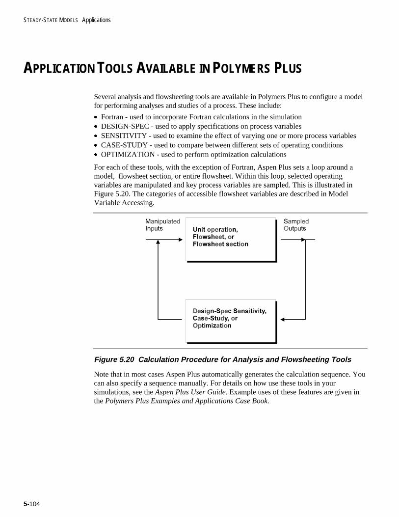
STEADY-STATE MODELS Applications
5x10⁴
APPLICATION TOOLS AVAILABLE IN POLYMERS PLUS
Several analysis and flowsheeting tools are available in Polymers Plus to configure a modelfor performing analyses and studies of a process. These include:
x Fortran - used to incorporate Fortran calculations in the simulationx DESIGN-SPEC - used to apply specifications on process variablesx SENSITIVITY - used to examine the effect of varying one or more process variablesx CASE-STUDY - used to compare between different sets of operating conditionsx OPTIMIZATION - used to perform optimization calculations
For each of these tools, with the exception of Fortran, Aspen Plus sets a loop around amodel, flowsheet section, or entire flowsheet. Within this loop, selected operatingvariables are manipulated and key process variables are sampled. This is illustrated inFigure 5.20. The categories of accessible flowsheet variables are described in ModelVariable Accessing.
Figure 5.20 Calculation Procedure for Analysis and Flowsheeting Tools
Note that in most cases Aspen Plus automatically generates the calculation sequence. Youcan also specify a sequence manually. For details on how use these tools in yoursimulations, see the Aspen Plus User Guide. Example uses of these features are given inthe Polymers Plus Examples and Applications Case Book.
Polymers Plus User Guide 5x10⁵
Fortran Fortran blocks provide a mechanism for you to incorporate Fortran statements into theflowsheet calculations. This can be used calculate and set input variables based on specialuser inputs. For this reason, Fortran blocks can be used as feed-forward controllers. Youcan also use Fortran blocks to calculate and write results to the Aspen Plus report, controlpanel, or external file.
To use this block you must specify which model variables to sample or manipulate, enterthe Fortran statements, and set the sequence in which the block must be executed duringthe flowsheet calculations.
An example use of a Fortran block as a feed-forward controller would be to hold theflowrate of a catalyst proportional to a monomer flow for a situation where that monomerflow varies.
DESIGN-SPEC Design-Spec blocks allow you to set a process variable which is normally calculatedduring the simulation. For each specification, you must identify which process variablecan be adjusted to meet that specification. For this reason, Design-Spec blocks can beused as feedback controllers.
To use this block you must specify which model variables must be fixed, what values theymust be fixed at, and which model input variables can be manipulated. You can includeFortran statements in Design-Spec blocks.
An example use of a Design-Spec block would be to set a maximum amount forimpurities in a product stream.
SENSITIVITY Sensitivity blocks provide a mechanism for you to analyze the effect of operatingvariables which you select on the process. This block generates a matrix of manipulatedvariables versus sampled variables. If there is more than one manipulated variable, thesensitivity analysis is performed for each combination of manipulated variables. It isrecommended that you use multiple Sensitivity blocks if you do not want to combine themanipulated variables.
To use this block you must specify which are the manipulated variables, which are thesampled variables, and how they must be tabulated. You can include Fortran statements inSensitivity blocks.
An example use of a Sensitivity block would be to determine the effect of reactortemperature or pressure on the polymer product properties.
STEADY-STATE MODELS Applications
5x10⁶
CASE-STUDY Case-Study blocks provide another mechanism for you to analyze the effect of operatingconditions on process variables. They allow you to make several runs in series for theentire flowsheet. Since a report is generated for the whole flowsheet for each case, you donot need to specify output variables to be sampled.
To use this block you must identify the case study variables, assign values for thesevariables, and specify reporting options.
An example use of Case-Study would be to investigate the effect of changing feedconditions and composition on key process variables.
OPTIMIZATION Optimization blocks provide a mechanism for you to minimize or maximize an objectivefunction calculated using key process variables. To define the objective function youwould use Fortran statements.
To use this block you must define the objective function, specify manipulated variables,and define constraints, if any.
An example use of Optimization would be to find the optimal reactor temperature to meetpolymer product property specifications while minimizing reaction medium viscosity.
MODEL VARIABLE ACCESSING
When using the various model analysis tools to perform sensitivity studies, optimizationstudies, case studies, or data fitting, or when applying design specifications, or adding in-lineFortran to a simulation model, users must access many different flowsheet variables. Theseflowsheet variables are grouped by type:
x Unit operation block variablex Stream variable (including polymer component attributes)x Reaction variablex Physical property variable
A list of such variables is given in Table 5.13.
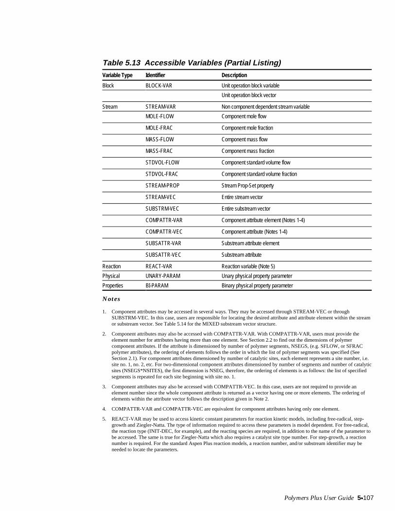
Polymers Plus User Guide 5x10⁷
Table 5.13 Accessible Variables (Partial Listing)Variable Type Identifier Description
Block BLOCK-VAR Unit operation block variable
Unit operation block vector
Stream STREAM-VAR Non component dependent stream variable
MOLE-FLOW Component mole flow
MOLE-FRAC Component mole fraction
MASS-FLOW Component mass flow
MASS-FRAC Component mass fraction
STDVOL-FLOW Component standard volume flow
STDVOL-FRAC Component standard volume fraction
STREAM-PROP Stream Prop-Set property
STREAM-VEC Entire stream vector
SUBSTRM-VEC Entire substream vector
COMPATTR-VAR Component attribute element (Notes 1-4)
COMPATTR-VEC Component attribute (Notes 1-4)
SUBSATTR-VAR Substream attribute element
SUBSATTR-VEC Substream attribute
Reaction REACT-VAR Reaction variable (Note 5)
Physical UNARY-PARAM Unary physical property parameter
Properties BI-PARAM Binary physical property parameter
Notes
1. Component attributes may be accessed in several ways. They may be accessed through STREAM-VEC or throughSUBSTRM-VEC. In this case, users are responsible for locating the desired attribute and attribute element within the streamor substream vector. See Table 5.14 for the MIXED substream vector structure.
2. Component attributes may also be accessed with COMPATTR-VAR. With COMPATTR-VAR, users must provide theelement number for attributes having more than one element. See Section 2.2 to find out the dimensions of polymercomponent attributes. If the attribute is dimensioned by number of polymer segments, NSEGS, (e.g. SFLOW, or SFRACpolymer attributes), the ordering of elements follows the order in which the list of polymer segments was specified (SeeSection 2.1). For component attributes dimensioned by number of catalytic sites, each element represents a site number, i.e.site no. 1, no. 2, etc. For two-dimensional component attributes dimensioned by number of segments and number of catalyticsites (NSEGS*NSITES), the first dimension is NSEG, therefore, the ordering of elements is as follows: the list of specifiedsegments is repeated for each site beginning with site no. 1.
3. Component attributes may also be accessed with COMPATTR-VEC. In this case, users are not required to provide anelement number since the whole component attribute is returned as a vector having one or more elements. The ordering ofelements within the attribute vector follows the description given in Note 2.
4. COMPATTR-VAR and COMPATTR-VEC are equivalent for component attributes having only one element.
5. REACT-VAR may be used to access kinetic constant parameters for reaction kinetic models, including free-radical, step-growth and Ziegler-Natta. The type of information required to access these parameters is model dependent. For free-radical,the reaction type (INIT-DEC, for example), and the reacting species are required, in addition to the name of the parameter tobe accessed. The same is true for Ziegler-Natta which also requires a catalyst site type number. For step-growth, a reactionnumber is required. For the standard Aspen Plus reaction models, a reaction number, and/or substream identifier may beneeded to locate the parameters.
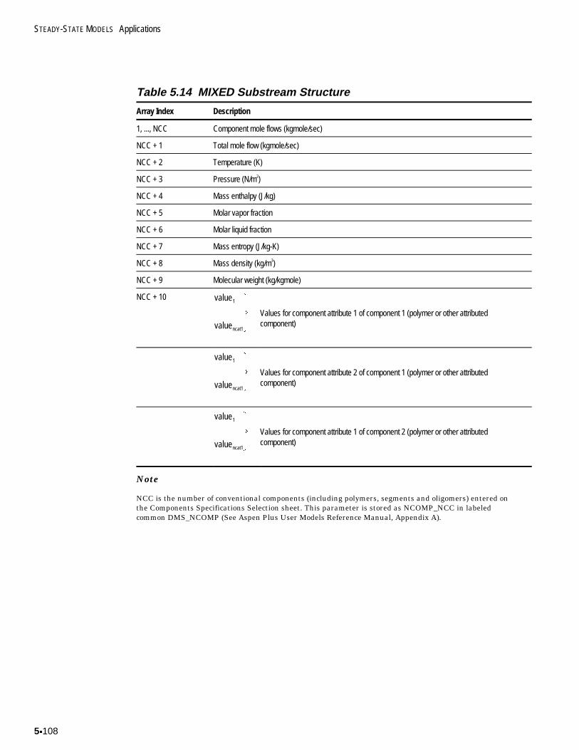
STEADY-STATE MODELS Applications
5x10⁸
Table 5.14 MIXED Substream Structure
Array Index Description
1, ..., NCC Component mole flows (kgmole/sec)
NCC + 1 Total mole flow (kgmole/sec)
NCC + 2 Temperature (K)
NCC + 3 Pressure (N/m2)
NCC + 4 Mass enthalpy (J/kg)
NCC + 5 Molar vapor fraction
NCC + 6 Molar liquid fraction
NCC + 7 Mass entropy (J/kg-K)
NCC + 8 Mass density (kg/m3)
NCC + 9 Molecular weight (kg/kgmole)
NCC + 10 value
value
1
ncat1
½
¾°
¿°
Values for component attribute 1 of component 1 (polymer or other attributedcomponent)
value
value
1
ncat1
½
¾°
¿°
Values for component attribute 2 of component 1 (polymer or other attributedcomponent)
value
value
1
ncat1
½
¾°
¿°
Values for component attribute 1 of component 2 (polymer or other attributedcomponent)
Note
NCC is the number of conventional components (including polymers, segments and oligomers) entered onthe Components Specifications Selection sheet. This parameter is stored as NCOMP_NCC in labeledcommon DMS_NCOMP (See Aspen Plus User Models Reference Manual, Appendix A).

Polymers Plus User Guide 5x10⁹
REFERENCES
Aspen Plus User Guide, Version 10.0, Aspen Technology, Inc. (1998).
Convergence and Optimization in Aspen Plus, Aspen Technology, Inc., Course notes.

STEADY-STATE MODELS Applications
5x110
Polymers Plus User Guide 6x1
6 RUN-TIME ENVIRONMENT
This chapter discusses various topics related to working in the Polymers Plusenvironment.
The topics covered include:
x Polymers Plus Architecturex Installation Issuesx Configuration Tipsx User Fortranx Troubleshooting Guidex Documentation and Online Help
POLYMERS PLUS ARCHITECTURE
Polymers Plus is a layered product. In other words, this product works in conjunction with amain program. This main program is Aspen Plus for steady-state simulation, or AspenCustom Modeler for dynamic simulation. Polymers Plus brings to these simulators thepolymer process technology in the form of component characterization, physical propertymodels and databanks, kinetic models, and the associated input forms. Figure 6.1 illustratesthe overall architecture.
As a result of this layered architecture the installation and configuration of Polymers Plusis closely tied to that of Aspen Plus for steady-state simulation and that of Aspen CustomModeler for dynamic simulation. In this chapter we will focus on topics related to theAspen Plus environment.
6
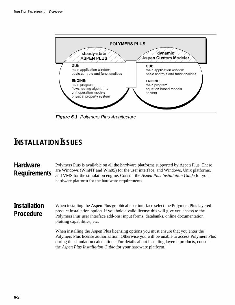
RUN-TIME ENVIRONMENT Overview
6x2
Figure 6.1 Polymers Plus Architecture
INSTALLATION ISSUES
HardwareRequirements
Polymers Plus is available on all the hardware platforms supported by Aspen Plus. Theseare Windows (WinNT and Win95) for the user interface, and Windows, Unix platforms,and VMS for the simulation engine. Consult the Aspen Plus Installation Guide for yourhardware platform for the hardware requirements.
InstallationProcedure
When installing the Aspen Plus graphical user interface select the Polymers Plus layeredproduct installation option. If you hold a valid license this will give you access to thePolymers Plus user interface add-ons: input forms, databanks, online documentation,plotting capabilities, etc.
When installing the Aspen Plus licensing options you must ensure that you enter thePolymers Plus license authorization. Otherwise you will be unable to access Polymers Plusduring the simulation calculations. For details about installing layered products, consultthe Aspen Plus Installation Guide for your hardware platform.
Polymers Plus User Guide 6x3
CONFIGURATION TIPS
Startup Files The information needed to launch the main Aspen Plus application window is recorded instartup files. These files define the type of simulation, default settings for the userinterface, hosts for the simulation engine, run settings, etc. One type of startup file is usedto define defaults for the type of simulation. This is the simulation template.
SimulationTemplates
Simulation templates are available to help you get started setting up your model. Thesetemplates typically contain options such as unit sets, physical property method selection,and Table File Format (TFF) selection for stream result tables. Polymer simulationtemplates are available. You can create your own personal template to allow fasterdefinition of a new simulation model. To use a simulation template, after starting AspenPlus, on the startup box select the template startup option. Then choose one of thepolymer simulation templates. This will automatically setup a global unit set, anappropriate polymer property method, and a polymer TFF for the stream tables.
To learn more about TFF files see the Aspen Plus System Management ReferenceManual.
USER FORTRAN
User FortranTemplates
There are several ways for you to customize your models by adding calculations inFortran. Section 2.4 described how to setup user a Prop-Set for calculating end-useproperties. Section 5.3 described how to setup user unit operation models, user kineticmodels, and user property models. Templates are available for your use in creating theFortran files used in these features. You will find these templates in the followinglocations:
Version Location
Windows %asptop%\user
UNIX $ASPDIR/user
VMS ASP$ROOT:[USER]
RUN-TIME ENVIRONMENT Overview
6x4
User FortranLinking
User Fortran calculations in the form of user routines are linked dynamically to PolymersPlus during a simulation. Within user Fortran, you will often access utilities locatedwithin Polymers Plus. In order to access these utilities, you will need to know the name ofthe object libraries where they are located. This applies to the utilities described inAppendix H. The name of the utility as shown in the example call sequence includes thename of the object library where it is located.
You can also create your own dynamic link libraries to hold your user Fortran files.Chapter 2 of Aspen Plus System Management, describes how to work with Fortran codemodifications.
TROUBLESHOOTING GUIDE
Following are tips to help you diagnose and resolve problems you may run into while settingup or running Polymers Plus.
User InterfaceProblems
Here is a list of symptoms relating problems you may encounter when using the userinterface. Possible causes and solutions are given for each symptom.
x The polymer input forms cannot be found on the GUIx A file created without using polymer features appears incomplete in the components
recordx Windows crashes during input specificationsx Windows crashes during simulation calculationsx Windows crashes after simulation is complete
Symptom: The polymer input forms cannot be found on the GUI.
Cause: The installation was not complete.
Solution: You must locate your installation CD and do an incremental installation ofPolymers Plus. Select the custom installation and choose the Polymers Plus layeredproduct.
�� or ��
Polymers Plus User Guide 6x5
Cause: Polymers Plus is installed but not enabled.
Solution: Enable Polymers Plus. From the Tools menu, select Options. On the Startuptab there is a box entitled Enable forms for layered products . Make sure you selectPolymers Plus.
Symptom: A file created without using polymer features appears incomplete in thecomponents record.
Cause: You visited the polymer record while creating the file, then later switched offPolymers Plus.
Solution: You must enable Polymers Plus (From the Tools menu, Select Options, clickon the Startup tab). In the Data Browser, select Polymers (Polymers will appear asincomplete), right mouse click, select Delete.
Symptom: Windows crashes during input specifications.
Cause: An invalid operation was performed either by the Aspen Plus program or byanother program running simultaneously.
Solution: Usually, when you crash, a backup file is created. Startup Aspen Plus again,then you should be able to recover your file. If the invalid operation was caused by AspenPlus, repeat the input steps that lead to the crash, verify that it is reproducible, and submitthe problem to Technical Support.
Symptom: Windows crashes during simulation calculations.
Cause: The simulation engine encountered an error that could not be transferred to theGUI.
Solution: Export an input summary. Run the input summary alone, then examine therun history for simulation errors. Change the input specifications associated with the errorand rerun.
�� or ��
RUN-TIME ENVIRONMENT Overview
6x6
Cause: Aspen Plus ran out of resources to create run files. This can happen especiallyfor large simulations. You may see error messages referring to the amount of virtualmemory available.
Solution: Free-up some disk space and run again. Also, consult the Aspen Plus SystemManagement Reference Manual, Chapter 3. An entire section is devoted to managingvirtual memory on Win95 and WinNT.
�� or ��
Cause: Aspen Plus ran out of memory to load dynamic link libraries.
Solution: Free-up some disk space or increase the amount of memory available to theapplication then run again.
Symptom: Windows crashes after simulation is complete.
Cause: Aspen Plus could not load the simulation results.
Solution: If you are running on a remote hosts, there may have been a communicationfailure at the end of the simulation calculations. You can submit the run again or you canmanually load the results file (.SUM) from the remote host.
�� or ��
If you are running on a local PC host, Aspen Plus may have run out of memory to load theresults. Free-up some disk space or increase the amount of memory available to theapplication and run again.
�� or ��
If the load failure was not due to any of the above, there may be some informationrecorded in the results file (.SUM) which is causing the problem. Contact TechnicalSupport and be prepared to supply the results file and/or your saved simulation file.
Polymers Plus User Guide 6x7
SimulationEngine Run-TimeProblems
Here is a list of symptoms relating to problems you may encounter with the simulationengine at run-time. Possible causes and solutions are given for each symptom.
x During simulation calculations an error message occurs for a license failurex A message box comes up stating that an error occurred in the Aspen Plus enginex A run history message appears referring to a dynamic load module errorx A run history message appears which refers to "Virtual Memory Exhausted"x After one run a subsequent run following an input change crashes
Symptom: During simulation calculations an error message occurs for a license failure.
Cause: The application could not find a valid free license to complete the simulation.
Solution: If the license error message refers to "Feature 10". This means that you do nothave a license for Aspen Plus itself. If you are using a licensed installation, then this couldbe a temporary license failure. This can happen for multi-user sites, or if you are using alicense manager located on a network. In that case, you simply need to try again later.
�� or ��
If you are using an installation with a single activator, then your license key file may becorrupted, the port where the activator is plugged in could be damaged, or the activatorcould be damaged. To correct your license key files, perform a license key installationagain. If the problem is your activator, contact Technical Support to have it replaced.
�� or ��
If the license error message refers to another feature number, you may still have run into atemporary license failure (see above). In that case, try again. If this was not a temporarylicense failure, then you created a simulation file which uses features for which you arenot licensed. If the message refers to "Feature 15", then you are trying to use PolymersPlus without a valid license. Other feature numbers refer to specific add-on products. Youmust contact AspenTech to obtain a valid Polymers Plus license.
Symptom: A message box comes up stating that an error occurred in the Aspen Plusengine.
Cause: See "Windows crashes during simulation calculations" under User InterfaceProblems. See also "After one run a subsequent run following an input change crashes" inthis section.
Solution: See "Windows crashes during simulation calculations" under User InterfaceProblems. See also "After one run a subsequent run following an input change crashes" inthis section.
RUN-TIME ENVIRONMENT Overview
6x8
Symptom: A run history message appears referring to a dynamic load module error.
Cause: Aspen Plus ran out of resources to load dynamic link libraries.
Solution: See "Windows crashes during simulation calculations" under User InterfaceProblems.
�� or ��
Cause: You are referencing user Fortran and do not have the compiled object file inyour working directory. The working directory is the location from which you opened anexisting file. If you created a file from a template or opened an existing file from a floppyor a write protected area (e.g. \xmp or \app) the working directory is as specified in ToolsOptions Startup.
Solution: Compile the user Fortran and place it in your run directory.
Symptom: A run history message appears which refers to "Virtual Memory Exhausted".
Cause: You ran out of virtual memory space to load the run files.
Solution: See the Aspen Plus System Management Reference Manual, Chapter 3 whichdiscusses virtual memory management.
Symptom: After one run a subsequent run following an input change crashes.
Cause: The problem size has changed as a result of the input or for other reasons AspenPlus unsuccessfully tried to reuse the previous run data space. Usually an error messageappears which states that a "Fatal error has been encountered".
Solution: Usually after the crash you should be able to recover your file and run with theinput change. To prevent this from happening for the same run, reinitialize the simulationbefore making repeated runs. This is still a problem which should be reported toTechnical Support.
Polymers Plus User Guide 6�9
DOCUMENTATION AND ONLINE HELP
Polymers Plus is available to you in electronic format. Your installation package includes adocumentation CD-ROM. On there you will find this Polymers Plus User Guide, Volumes Iand II, and also the Polymers Plus Examples and Applications Case Book. These aredelivered in the Portable Document Format (PDF). They can be read using the AdobeAcrobat Reader�.
In addition, you will find Polymers Plus online help from within the application. Thisonline help can be accessed from the main application window Help menu Help TopicsContents. In the Help contents go to "Using Polymers Plus" for step-by-step proceduralinstructions. Online Help can also be accessed through the fully integrated search indexand Find menu. You can also request help from within the polymer input forms using thehelp key, F1, or using the "What's This" button
.
REFERENCES
Aspen Plus Installation Guides for Windows, Unix and VMS, Version 10.0, AspenTechnology, Inc. (1998).
Aspen Plus Reference Manual, "System Management", Aspen Technology, Inc. (1998).
Aspen Plus User Guide, Version 10.0, Aspen Technology, Inc. (1998).

RUN-TIME ENVIRONMENT Overview
6x10
Polymers Plus User Guide Ax1
A COMPONENT DATABANKS
This appendix documents the Polymers Plus component databanks. There are currentlytwo databanks available:
x POLYMER Databank - containing polymer pure component parameters (Ax2)x SEGMENT Databank - containing segment pure component parameters (Ax8)
In addition users may retrieve parameters from the Aspen Plus databanks.
PURE COMPONENT DATABANK
The pure component databanks contain pure component data for over 1500 species.Typically components such as monomers, solvents, catalysts, initiators, etc. would beretrieved from the pure component databanks. The parameters in these databanks includethose listed in Table A.1.
A
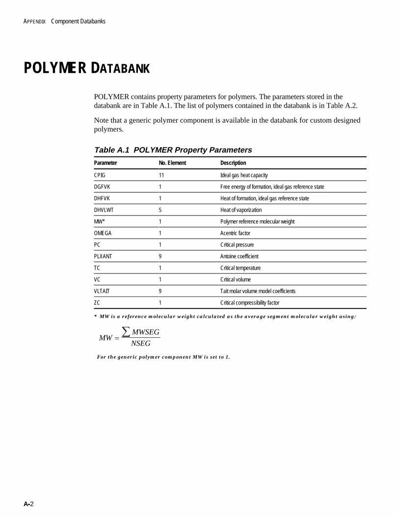
APPENDIX Component Databanks
Ax2
POLYMER DATABANK
POLYMER contains property parameters for polymers. The parameters stored in thedatabank are in Table A.1. The list of polymers contained in the databank is in Table A.2.
Note that a generic polymer component is available in the databank for custom designedpolymers.
Table A.1 POLYMER Property Parameters
Parameter No. Element Description
CPIG 11 Ideal gas heat capacity
DGFVK 1 Free energy of formation, ideal gas reference state
DHFVK 1 Heat of formation, ideal gas reference state
DHVLWT 5 Heat of vaporization
MW* 1 Polymer reference molecular weight
OMEGA 1 Acentric factor
PC 1 Critical pressure
PLXANT 9 Antoine coefficient
TC 1 Critical temperature
VC 1 Critical volume
VLTAIT 9 Tait molar volume model coefficients
ZC 1 Critical compressibility factor
* MW is a reference molecular weight calculated as the average segment molecular weight using:
MWMWSEG
NSEG ¦
For the generic polymer component MW is set to 1.
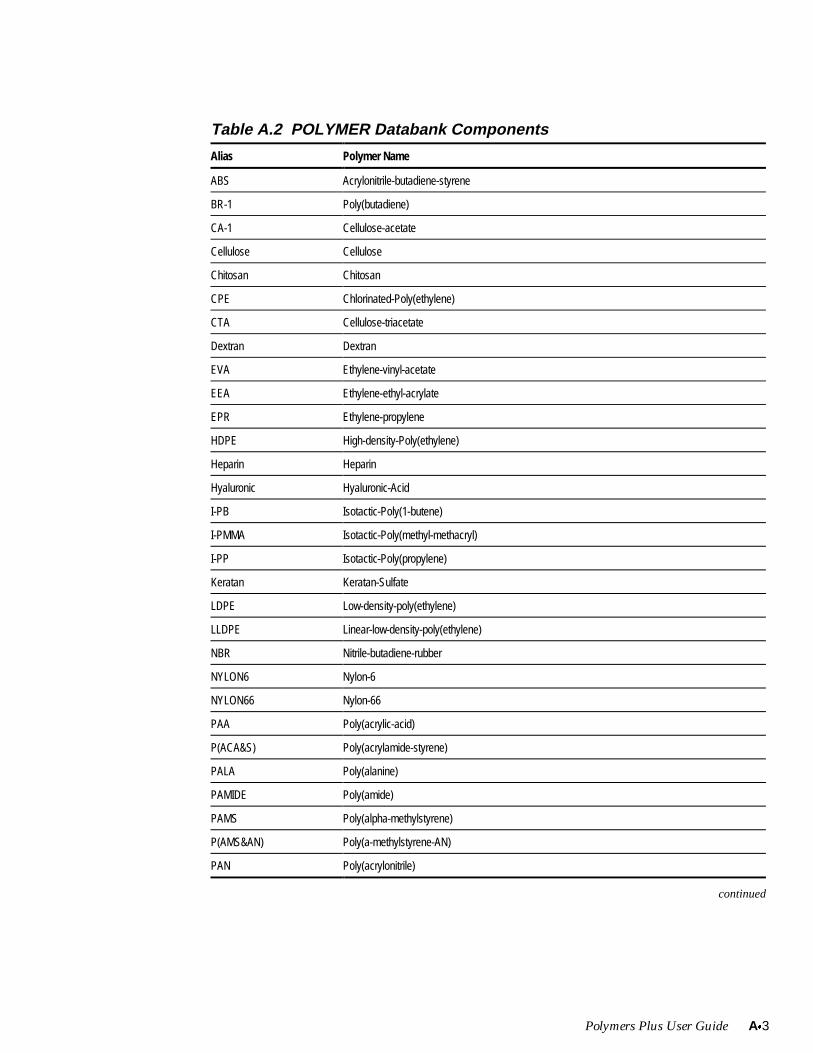
Polymers Plus User Guide Ax3
Table A.2 POLYMER Databank Components
Alias Polymer Name
ABS Acrylonitrile-butadiene-styrene
BR-1 Poly(butadiene)
CA-1 Cellulose-acetate
Cellulose Cellulose
Chitosan Chitosan
CPE Chlorinated-Poly(ethylene)
CTA Cellulose-triacetate
Dextran Dextran
EVA Ethylene-vinyl-acetate
EEA Ethylene-ethyl-acrylate
EPR Ethylene-propylene
HDPE High-density-Poly(ethylene)
Heparin Heparin
Hyaluronic Hyaluronic-Acid
I-PB Isotactic-Poly(1-butene)
I-PMMA Isotactic-Poly(methyl-methacryl)
I-PP Isotactic-Poly(propylene)
Keratan Keratan-Sulfate
LDPE Low-density-poly(ethylene)
LLDPE Linear-low-density-poly(ethylene)
NBR Nitrile-butadiene-rubber
NYLON6 Nylon-6
NYLON66 Nylon-66
PAA Poly(acrylic-acid)
P(ACA&S) Poly(acrylamide-styrene)
PALA Poly(alanine)
PAMIDE Poly(amide)
PAMS Poly(alpha-methylstyrene)
P(AMS&AN) Poly(a-methylstyrene-AN)
PAN Poly(acrylonitrile)
continued
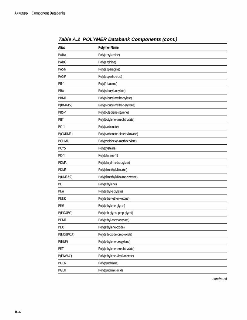
APPENDIX Component Databanks
Ax4
Table A.2 POLYMER Databank Components (cont.)
Alias Polymer Name
PARA Poly(acrylamide)
PARG Poly(arginine)
PASN Poly(asparagine)
PASP Poly(aspartic-acid)
PB-1 Poly(1-butene)
PBA Poly(n-butyl-acrylate)
PBMA Poly(n-butyl-methacrylate)
P(BMA&S) Poly(n-butyl-methac-styrene)
PBS-1 Poly(butadiene-styrene)
PBT Poly(butylene-terephthalate)
PC-1 Poly(carbonate)
P(C&DMS) Poly(carbonate-dimet-siloxane)
PCHMA Poly(cyclohexyl-methacrylate)
PCYS Poly(cysteine)
PD-1 Poly(decene-1)
PDMA Poly(decyl-methacrylate)
PDMS Poly(dimethylsiloxane)
P(DMS&S) Poly(dimethylsiloxane-styrene)
PE Poly(ethylene)
PEA Poly(ethyl-acrylate)
PEEK Poly(ether-ether-ketone)
PEG Poly(ethylene-glycol)
P(EG&PG) Poly(eth-glycol-prop-glycol)
PEMA Poly(ethyl-methacrylate)
PEO Poly(ethylene-oxide)
P(EO&POX) Poly(eth-oxide-prop-oxide)
P(E&P) Poly(ethylene-propylene)
PET Poly(ethylene-terephthalate)
P(E&VAC) Poly(ethylene-vinyl-acetate)
PGLN Poly(glutamine)
PGLU Poly(glutamic-acid)
continued
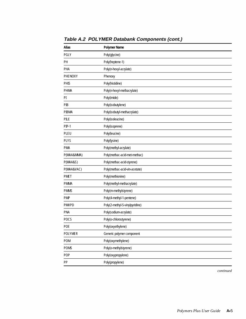
Polymers Plus User Guide Ax5
Table A.2 POLYMER Databank Components (cont.)
Alias Polymer Name
PGLY Poly(glycine)
PH Poly(heptene-1)
PHA Poly(n-hexyl-acrylate)
PHENOXY Phenoxy
PHIS Poly(histidine)
PHMA Poly(n-hexyl-methacrylate)
PI Poly(imide)
PIB Poly(isobutylene)
PIBMA Poly(isobutyl-methacrylate)
PILE Poly(isoleucine)
PIP-1 Poly(isoprene)
PLEU Poly(leucine)
PLYS Poly(lysine)
PMA Poly(methyl-acrylate)
P(MAA&MMA) Poly(methac-acid-met-methac)
P(MAA&S) Poly(methac-acid-styrene)
P(MAA&VAC) Poly(methac-acid-vin-acetate)
PMET Poly(methionine)
PMMA Poly(methyl-methacrylate)
PMMS Poly(m-methylstyrene)
PMP Poly(4-methyl-1-pentene)
PMVPD Poly(2-methyl-5-vinylpyridine)
PNA Poly(sodium-acrylate)
POCS Poly(o-chlorostyrene)
POE Poly(oxyethylene)
POLYMER Generic polymer component
POM Poly(oxymethylene)
POMS Poly(o-methylstyrene)
POP Poly(oxypropylene)
PP Poly(propylene)
continued
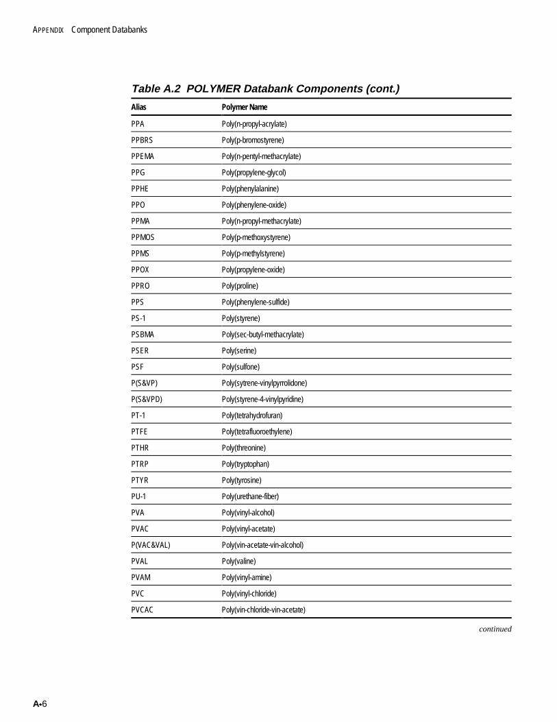
APPENDIX Component Databanks
Ax6
Table A.2 POLYMER Databank Components (cont.)
Alias Polymer Name
PPA Poly(n-propyl-acrylate)
PPBRS Poly(p-bromostyrene)
PPEMA Poly(n-pentyl-methacrylate)
PPG Poly(propylene-glycol)
PPHE Poly(phenylalanine)
PPO Poly(phenylene-oxide)
PPMA Poly(n-propyl-methacrylate)
PPMOS Poly(p-methoxystyrene)
PPMS Poly(p-methylstyrene)
PPOX Poly(propylene-oxide)
PPRO Poly(proline)
PPS Poly(phenylene-sulfide)
PS-1 Poly(styrene)
PSBMA Poly(sec-butyl-methacrylate)
PSER Poly(serine)
PSF Poly(sulfone)
P(S&VP) Poly(sytrene-vinylpyrrolidone)
P(S&VPD) Poly(styrene-4-vinylpyridine)
PT-1 Poly(tetrahydrofuran)
PTFE Poly(tetrafluoroethylene)
PTHR Poly(threonine)
PTRP Poly(tryptophan)
PTYR Poly(tyrosine)
PU-1 Poly(urethane-fiber)
PVA Poly(vinyl-alcohol)
PVAC Poly(vinyl-acetate)
P(VAC&VAL) Poly(vin-acetate-vin-alcohol)
PVAL Poly(valine)
PVAM Poly(vinyl-amine)
PVC Poly(vinyl-chloride)
PVCAC Poly(vin-chloride-vin-acetate)
continued
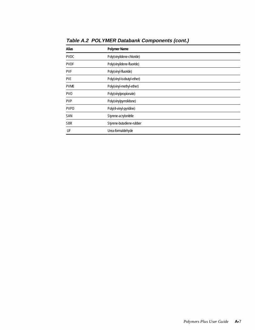
Polymers Plus User Guide Ax7
Table A.2 POLYMER Databank Components (cont.)
Alias Polymer Name
PVDC Poly(vinylidene-chloride)
PVDF Poly(vinylidene-fluoride)
PVF Poly(vinyl-fluoride)
PVI Poly(vinyl-isobutyl-ether)
PVME Poly(vinyl-methyl-ether)
PVO Poly(vinylpropionate)
PVP Poly(vinylpyrrolidone)
PVPD Poly(4-vinyl-pyridine)
SAN Styrene-acrylonitrile
SBR Styrene-butadiene-rubber
UF Urea-formaldehyde
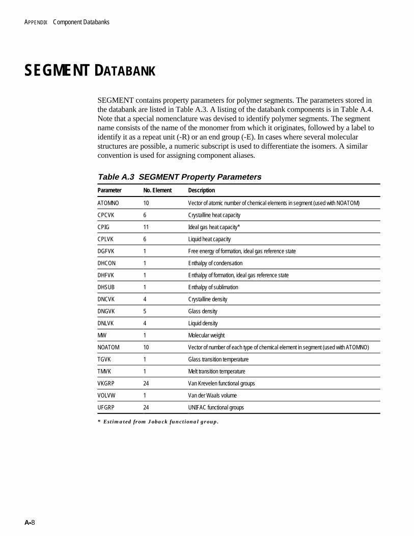
APPENDIX Component Databanks
Ax8
SEGMENT DATABANK
SEGMENT contains property parameters for polymer segments. The parameters stored inthe databank are listed in Table A.3. A listing of the databank components is in Table A.4.Note that a special nomenclature was devised to identify polymer segments. The segmentname consists of the name of the monomer from which it originates, followed by a label toidentify it as a repeat unit (-R) or an end group (-E). In cases where several molecularstructures are possible, a numeric subscript is used to differentiate the isomers. A similarconvention is used for assigning component aliases.
Table A.3 SEGMENT Property Parameters
Parameter No. Element Description
ATOMNO 10 Vector of atomic number of chemical elements in segment (used with NOATOM)
CPCVK 6 Crystalline heat capacity
CPIG 11 Ideal gas heat capacity*
CPLVK 6 Liquid heat capacity
DGFVK 1 Free energy of formation, ideal gas reference state
DHCON 1 Enthalpy of condensation
DHFVK 1 Enthalpy of formation, ideal gas reference state
DHSUB 1 Enthalpy of sublimation
DNCVK 4 Crystalline density
DNGVK 5 Glass density
DNLVK 4 Liquid density
MW 1 Molecular weight
NOATOM 10 Vector of number of each type of chemical element in segment (used with ATOMNO)
TGVK 1 Glass transition temperature
TMVK 1 Melt transition temperature
VKGRP 24 Van Krevelen functional groups
VOLVW 1 Van der Waals volume
UFGRP 24 UNIFAC functional groups
* Estimated from Joback functional group.
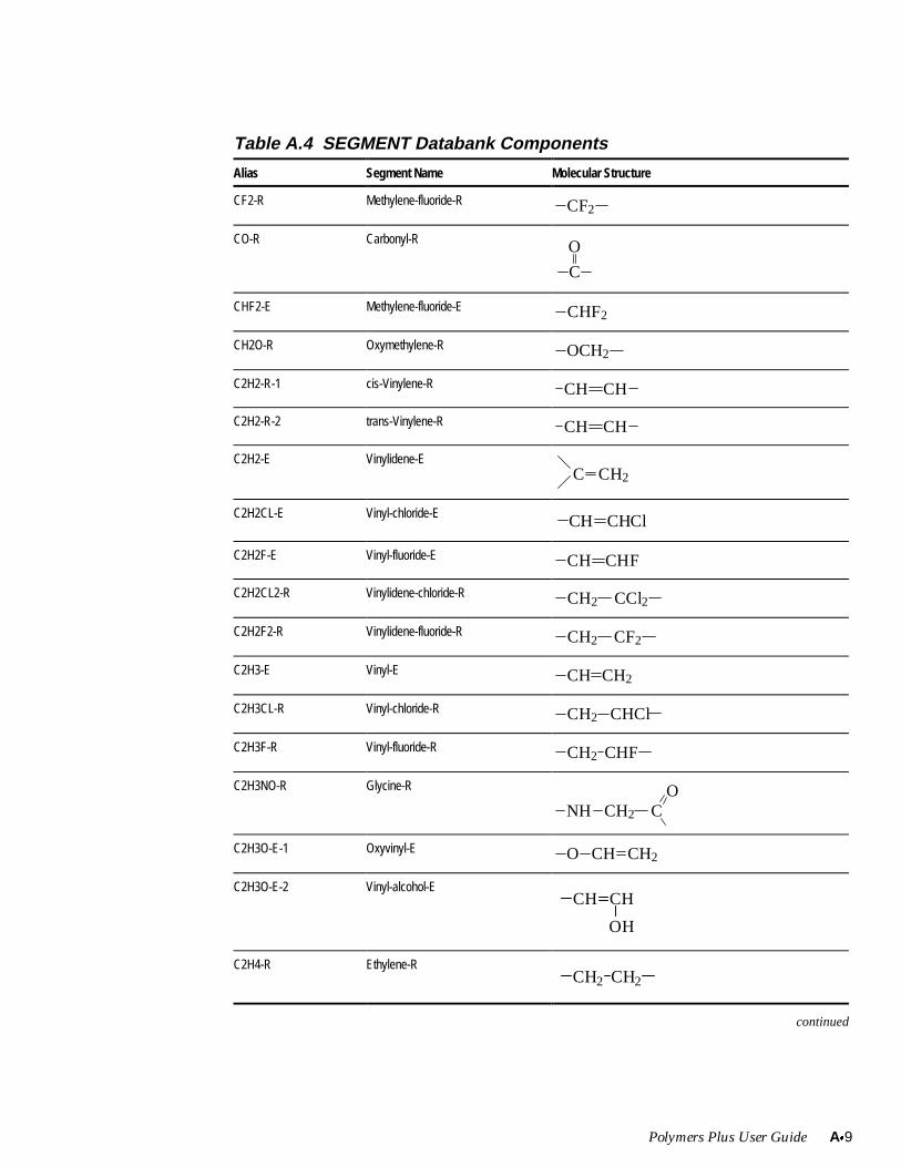
Polymers Plus User Guide Ax9
Table A.4 SEGMENT Databank Components
Alias Segment Name Molecular Structure
CF2-R Methylene-fluoride-R CF2
CO-R Carbonyl-R
C
O
CHF2-E Methylene-fluoride-E CHF2
CH2O-R Oxymethylene-R OCH2
C2H2-R-1 cis-Vinylene-R CH CH
C2H2-R-2 trans-Vinylene-R CH CH
C2H2-E Vinylidene-EC CH2
C2H2CL-E Vinyl-chloride-E CH CHCl
C2H2F-E Vinyl-fluoride-E CH CHF
C2H2CL2-R Vinylidene-chloride-R CH2 CCl2
C2H2F2-R Vinylidene-fluoride-R CH2 CF2
C2H3-E Vinyl-E CH CH2
C2H3CL-R Vinyl-chloride-R CH2 CHCl
C2H3F-R Vinyl-fluoride-R CH2 CHF
C2H3NO-R Glycine-R
CH2NHO
C
C2H3O-E-1 Oxyvinyl-E O CH2CH
C2H3O-E-2 Vinyl-alcohol-ECH CH
OH
C2H4-R Ethylene-RCH2 CH2
continued
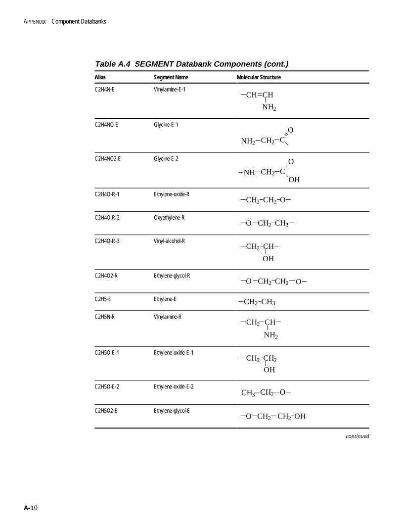
APPENDIX Component Databanks
Ax10
Table A.4 SEGMENT Databank Components (cont.)
Alias Segment Name Molecular Structure
C2H4N-E Vinylamine-E-1CH CH
NH2
C2H4NO-E Glycine-E-1
NH2 CH2 CO
C2H4NO2-E Glycine-E-2
CH2 CO
NHOH
C2H4O-R-1 Ethylene-oxide-RCH2 CH2 O
C2H4O-R-2 Oxyethylene-RCH2 CH2O
C2H4O-R-3 Vinyl-alcohol-RCH2 CH
OH
C2H4O2-R Ethylene-glycol-RCH2 CH2O O
C2H5-E Ethylene-E CH2 CH3
C2H5N-R Vinylamine-RCH2 CH
NH2
C2H5O-E-1 Ethylene-oxide-E-1CH2 CH2
OH
C2H5O-E-2 Ethylene-oxide-E-2CH2CH3 O
C2H5O2-E Ethylene-glycol-ECH2O CH2 OH
continued
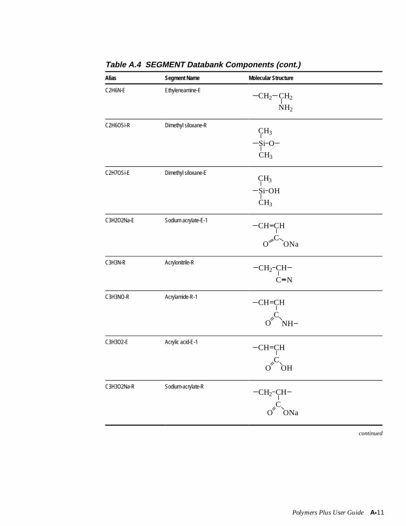
Polymers Plus User Guide Ax11
Table A.4 SEGMENT Databank Components (cont.)
Alias Segment Name Molecular Structure
C2H6N-E Ethyleneamine-ECH2 CH2
NH2
C2H6OSi-R Dimethyl siloxane-RCH3
Si O
CH3
C2H7OSi-E Dimethyl siloxane-ECH3
Si OH
CH3
C3H2O2Na-E Sodium acrylate-E-1CH CH
CO ONa
C3H3N-R Acrylonitrile-RCHCH2
C N
C3H3NO-R Acrylamide-R-1CH CH
CO NH
C3H3O2-E Acrylic acid-E-1CH CH
CO OH
C3H3O2Na-R Sodium-acrylate-R
CO
CHCH2
ONa
continued
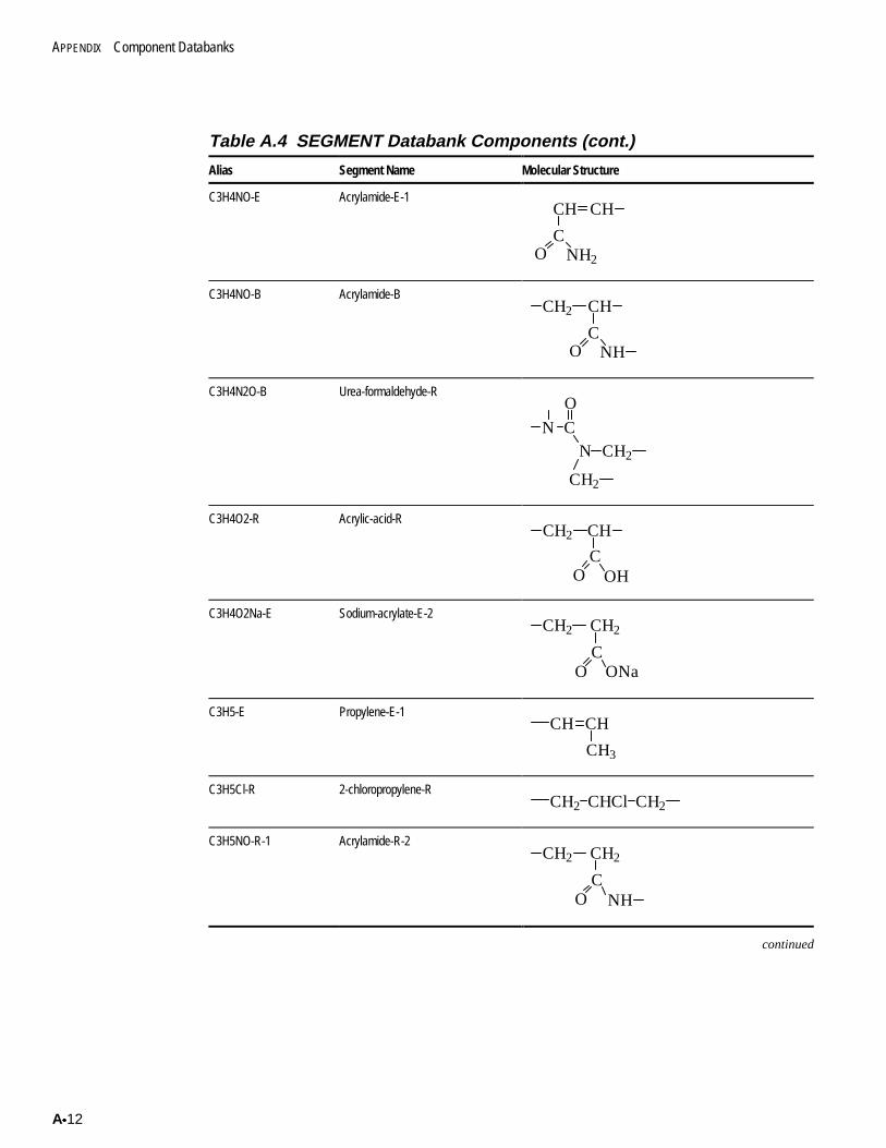
APPENDIX Component Databanks
Ax12
Table A.4 SEGMENT Databank Components (cont.)
Alias Segment Name Molecular Structure
C3H4NO-E Acrylamide-E-1
CO
CH CH
NH2
C3H4NO-B Acrylamide-B
CO
CHCH2
NH
C3H4N2O-B Urea-formaldehyde-R
CH2
N C
O
N
CH2
C3H4O2-R Acrylic-acid-RCH2
O
CH
COH
C3H4O2Na-E Sodium-acrylate-E-2CH2
OC
ONa
CH2
C3H5-E Propylene-E-1CH CH
CH3
C3H5Cl-R 2-chloropropylene-RCH2 CHCl CH2
C3H5NO-R-1 Acrylamide-R-2CH2
OC
CH2
NH
continued
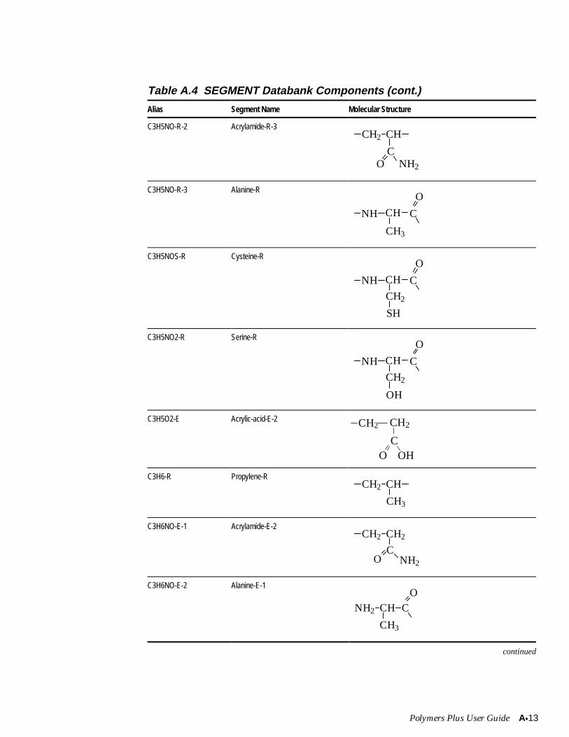
Polymers Plus User Guide Ax13
Table A.4 SEGMENT Databank Components (cont.)
Alias Segment Name Molecular Structure
C3H5NO-R-2 Acrylamide-R-3CH2 CH
OC
NH2
C3H5NO-R-3 Alanine-R
CHNH C
O
CH3
C3H5NOS-R Cysteine-R
CHNH C
O
CH2
SH
C3H5NO2-R Serine-R
CHNH C
O
CH2
OH
C3H5O2-E Acrylic-acid-E-2
CO OH
CH2 CH2
C3H6-R Propylene-RCH2 CH
CH3
C3H6NO-E-1 Acrylamide-E-2CH2 CH2
CO NH2
C3H6NO-E-2 Alanine-E-1
NH2 CH C
O
CH3
continued
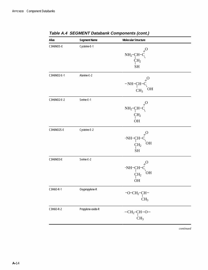
APPENDIX Component Databanks
Ax14
Table A.4 SEGMENT Databank Components (cont.)
Alias Segment Name Molecular Structure
C3H6NOS-E Cysteine-E-1
NH2 CH C
O
CH2
SH
C3H6NO2-E-1 Alanine-E-2O
CH CNHOHCH3
C3H6NO2-E-2 Serine-E-1O
CH CNH2
CH2
OH
C3H6NO2S-E Cysteine-E-2O
CH CNH
CH2OH
SH
C3H6NO3-E Serine-E-2O
CH CNH
CH2OH
OH
C3H6O-R-1 Oxypropylene-RO CH2 CH
CH3
C3H6O-R-2 Propylene-oxide-R
CH3
OCH2 CH
continued
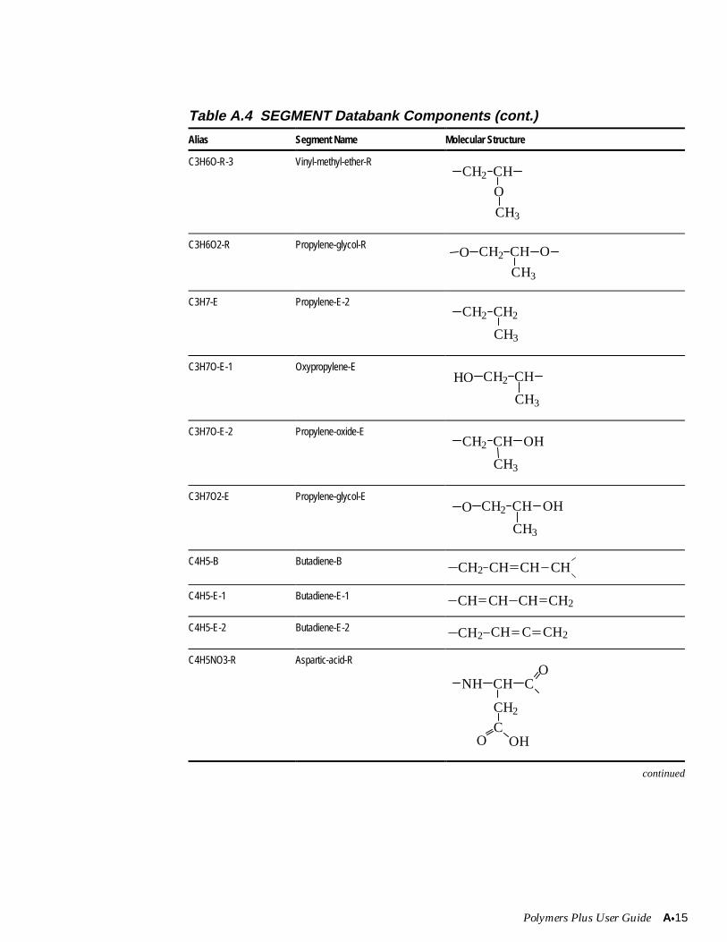
Polymers Plus User Guide Ax15
Table A.4 SEGMENT Databank Components (cont.)
Alias Segment Name Molecular Structure
C3H6O-R-3 Vinyl-methyl-ether-R
CH3
O
CH2 CH
C3H6O2-R Propylene-glycol-R
CH3
OCH2 CHO
C3H7-E Propylene-E-2
CH3
CH2 CH2
C3H7O-E-1 Oxypropylene-ECH2 CH
CH3
HO
C3H7O-E-2 Propylene-oxide-ECH2 CH
CH3
OH
C3H7O2-E Propylene-glycol-ECH2 CH
CH3
OHO
C4H5-B Butadiene-B CH2 CH CH CH
C4H5-E-1 Butadiene-E-1 CH CH2CH CH
C4H5-E-2 Butadiene-E-2 CH2CH2 CH C
C4H5NO3-R Aspartic-acid-R
NH CH CO
CH2
CO OH
continued
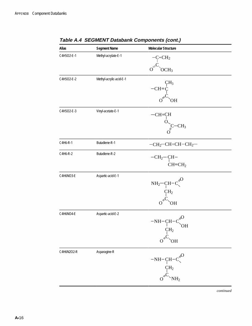
APPENDIX Component Databanks
Ax16
Table A.4 SEGMENT Databank Components (cont.)
Alias Segment Name Molecular Structure
C4H5O2-E-1 Methyl-acrylate-E-1
CO OCH3
CH2C
C4H5O2-E-2 Methyl-acrylic-acid-E-1
CO OH
CCH3
CH
C4H5O2-E-3 Vinyl-acetate-E-1
OCH3
CH CH
CO
C4H6-R-1 Butadiene-R-1 CH CHCH2 CH2
C4H6-R-2 Butadiene-R-2CHCH2
CH CH2
C4H6NO3-E Aspartic-acid-E-1
CH
CH2
CO OH
CO
NH2
C4H6NO4-E Aspartic-acid-E-2
CH
CH2
CO OH
CO
NHOH
C4H6N2O2-R Asparagine-R
CH
CH2
CO
CO
NH
NH2
continued
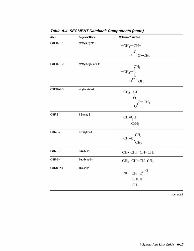
Polymers Plus User Guide Ax17
Table A.4 SEGMENT Databank Components (cont.)
Alias Segment Name Molecular Structure
C4H6O2-R-1 Methyl-acrylate-RCH
CO
CH2
O CH3
C4H6O2-R-2 Methyl acrylic-acid-R
O
CH2
CH3
C
COH
C4H6O2-R-3 Vinyl-acetate-R
O
CH2 CH
OC CH3
C4H7-E-1 1-Butene-ECH CH
C2H5
C4H7-E-2 Isobutylene-E
CH CCH3
CH3
C4H7-E-3 Butadiene-E-3 CH CH2CH2 CH2
C4H7-E-4 Butadiene-E-4 CHCH2 CH CH3
C4H7NO2-R Threonine-R
NH CH CO
CHOH
CH3
continued
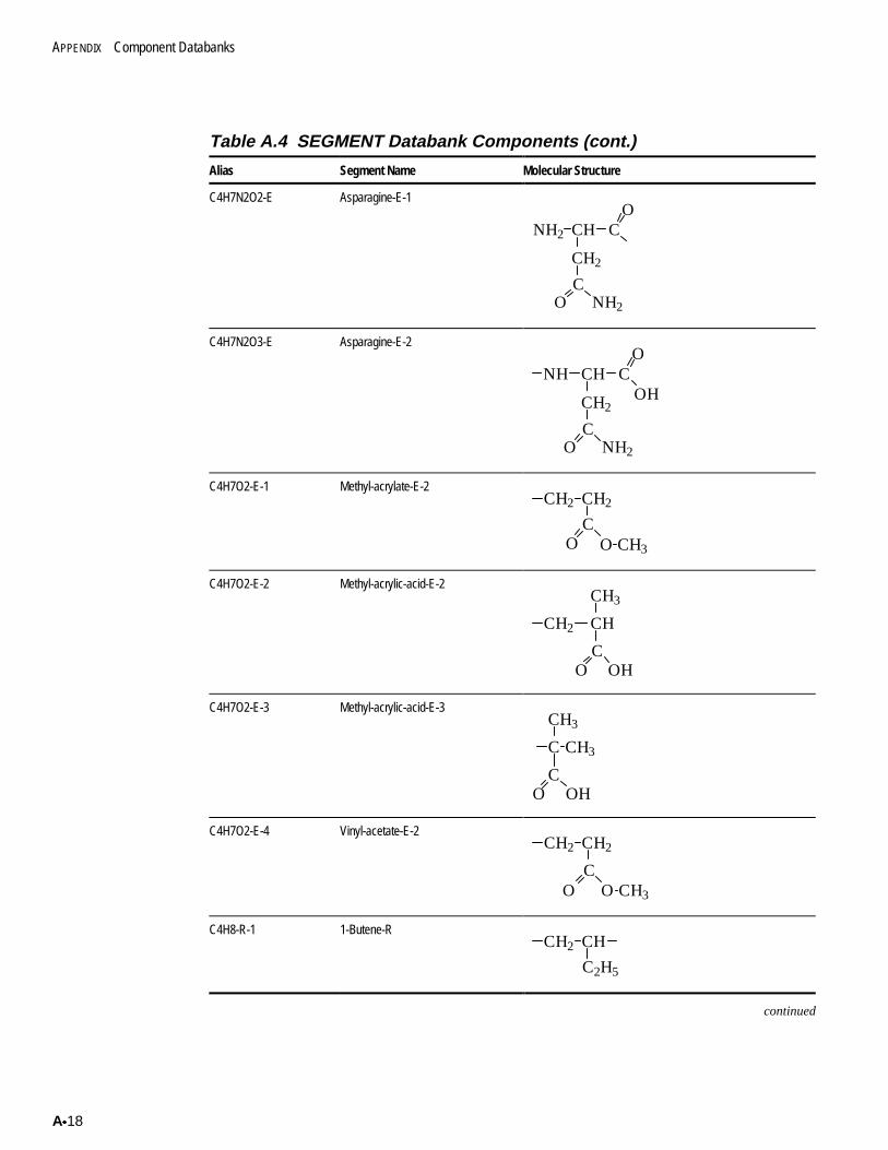
APPENDIX Component Databanks
Ax18
Table A.4 SEGMENT Databank Components (cont.)
Alias Segment Name Molecular Structure
C4H7N2O2-E Asparagine-E-1
NH2
CH2
CO
NH2 CH CO
C4H7N2O3-E Asparagine-E-2
NH2
CH2
CO
CO
CHNHOH
C4H7O2-E-1 Methyl-acrylate-E-2CH2 CH2
CO O CH3
C4H7O2-E-2 Methyl-acrylic-acid-E-2CH3
CHCH2
O OHC
C4H7O2-E-3 Methyl-acrylic-acid-E-3CH3
O OH
C CH3
C
C4H7O2-E-4 Vinyl-acetate-E-2CH2 CH2
CO O CH3
C4H8-R-1 1-Butene-RCH2 CH
C2H5
continued
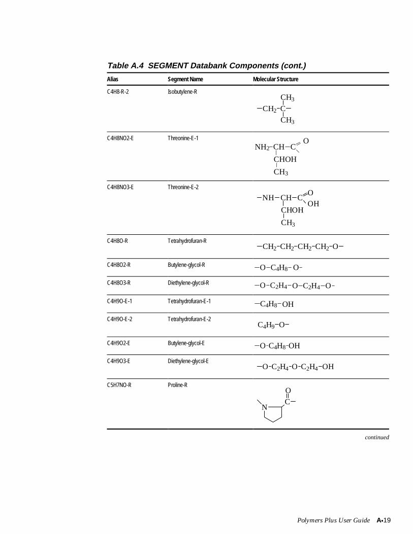
Polymers Plus User Guide Ax19
Table A.4 SEGMENT Databank Components (cont.)
Alias Segment Name Molecular Structure
C4H8-R-2 Isobutylene-R
CH2 C
CH3
CH3
C4H8NO2-E Threonine-E-1
CHNH2 CO
CHOH
CH3
C4H8NO3-E Threonine-E-2
CH CO
CHOH
CH3
NHOH
C4H8O-R Tetrahydrofuran-RCH2 CH2 CH2 CH2 O
C4H8O2-R Butylene-glycol-R O C4H8 O
C4H8O3-R Diethylene-glycol-R O C2H4 O C2H4 O
C4H9O-E-1 Tetrahydrofuran-E-1 C4H8 OH
C4H9O-E-2 Tetrahydrofuran-E-2C4H9 O
C4H9O2-E Butylene-glycol-E O C4H8 OH
C4H9O3-E Diethylene-glycol-EO C2H4 O C2H4 OH
C5H7NO-R Proline-R
NC
O
continued
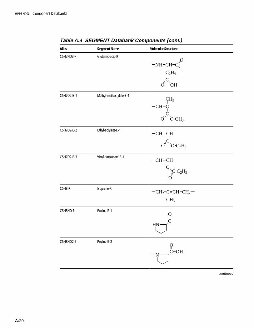
APPENDIX Component Databanks
Ax20
Table A.4 SEGMENT Databank Components (cont.)
Alias Segment Name Molecular Structure
C5H7NO3-R Glutamic-acid-R
NH CH CO
C2H4
CO OH
C5H7O2-E-1 Methyl-methacrylate-E-1CH3
CCH
CO O CH3
C5H7O2-E-2 Ethyl-acrylate-E-1CH CH
CO O C2H5
C5H7O2-E-3 Vinyl-propionate-E-1CH CH
OC C2H5
O
C5H8-R Isoprene-RCH2 C CH CH2
CH3
C5H8NO-E Proline-E-1
HNC
O
C5H8NO2-E Proline-E-2O
NC OH
continued
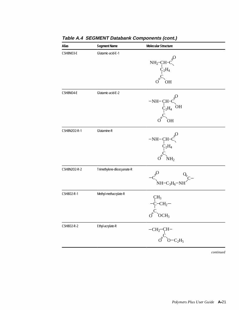
Polymers Plus User Guide Ax21
Table A.4 SEGMENT Databank Components (cont.)
Alias Segment Name Molecular Structure
C5H8NO3-E Glutamic-acid-E-1
NH2 CH CO
C2H4
CO OH
C5H8NO4-E Glutamic-acid-E-2
NHO
C2H4
CO OH
CH COH
C5H8N2O2-R-1 Glutamine-R
NHO
C2H4
CO
CH C
NH2
C5H8N2O2-R-2 Trimethylene-diisocyanate-RO
NH C3H6 NHC C
O
C5H8O2-R-1 Methyl-methacrylate-R
C
CH3
CH2
CO OCH3
C5H8O2-R-2 Ethyl-acrylate-R
CO O C2H5
CHCH2
continued
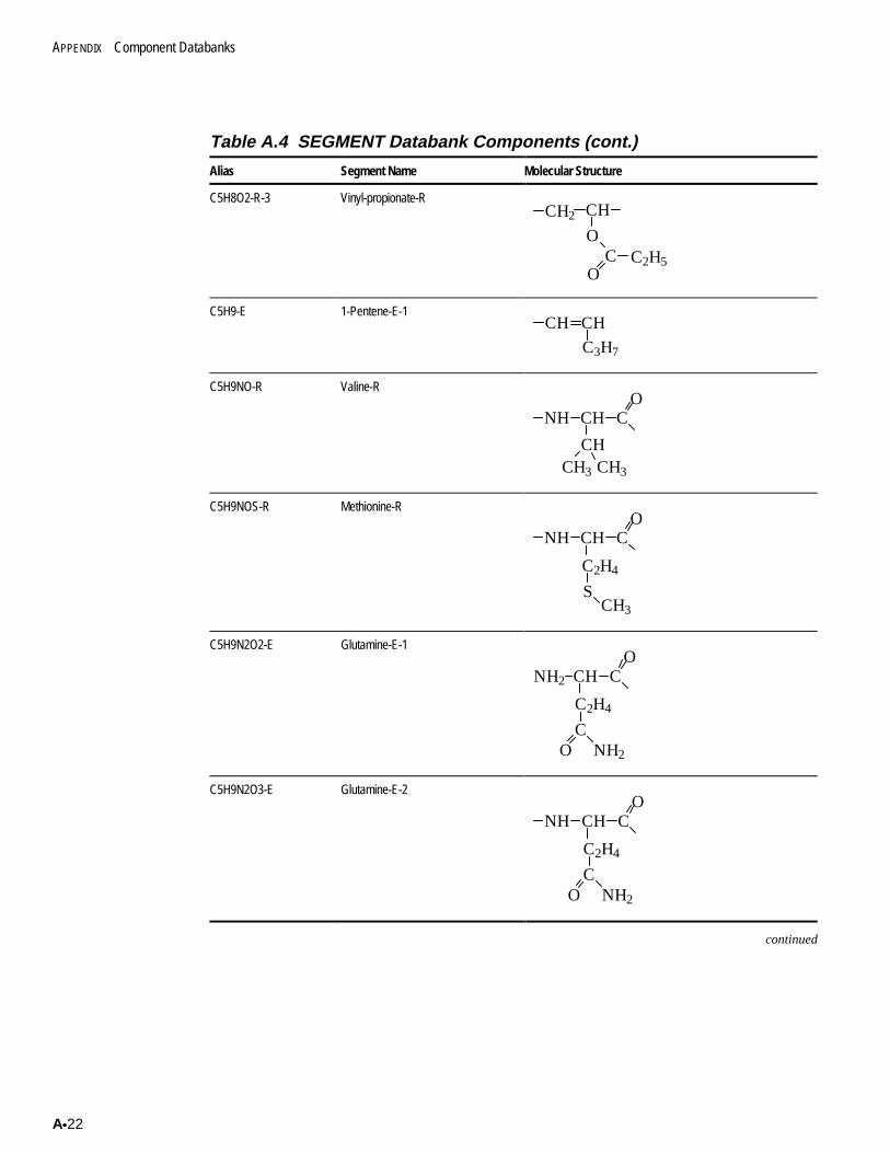
APPENDIX Component Databanks
Ax22
Table A.4 SEGMENT Databank Components (cont.)
Alias Segment Name Molecular Structure
C5H8O2-R-3 Vinyl-propionate-R
OC2H5
CHCH2
CO
C5H9-E 1-Pentene-E-1CH CH
C3H7
C5H9NO-R Valine-R
NH CH CO
CH3 CH3
CH
C5H9NOS-R Methionine-R
NH CH CO
CH3
C2H4
S
C5H9N2O2-E Glutamine-E-1O
C2H4
NH2 CCH
CO NH2
C5H9N2O3-E Glutamine-E-2O
C2H4
CO NH2
CCHNH
continued
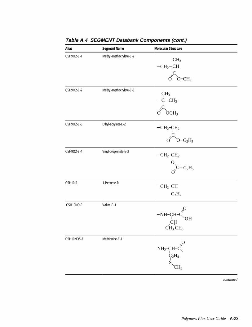
Polymers Plus User Guide Ax23
Table A.4 SEGMENT Databank Components (cont.)
Alias Segment Name Molecular Structure
C5H9O2-E-1 Methyl-methacrylate-E-2
O CH3
CO
CH3
CH2 CH
C5H9O2-E-2 Methyl-methacrylate-E-3
O
CH3
C
C
CH3
OCH3
C5H9O2-E-3 Ethyl-acrylate-E-2CH2 CH2
CO O C2H5
C5H9O2-E-4 Vinyl-propionate-E-2CH2 CH2
O
OC2H5C
C5H10-R 1-Pentene-RCH2 CH
C3H7
C5H10NO-E Valine-E-1
NH CH CO
OHCH
CH3 CH3
C5H10NOS-E Methionine-E-1O
CH3
CH CNH2
C2H4
S
continued
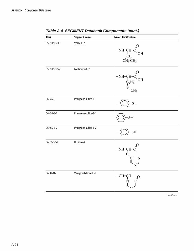
APPENDIX Component Databanks
Ax24
Table A.4 SEGMENT Databank Components (cont.)
Alias Segment Name Molecular Structure
C5H10NO2-E Valine-E-2
NH CH CO
OHCH
CH3 CH3
C5H10NO2S-E Methionine-E-2
NH CH CO
OH
CH3
C2H4
S
C6H4S-R Phenylene-sulfide-R
S
C6H5S-E-1 Phenylene-sulfide-E-1
S
C6H5S-E-2 Phenylene-sulfide-E-2
SH
C6H7N3O-R Histidine-R
NH CH CC
O
NC
N
C6H8NO-E Vinylpyrrolidnone-E-1O
CN
CHCH
continued
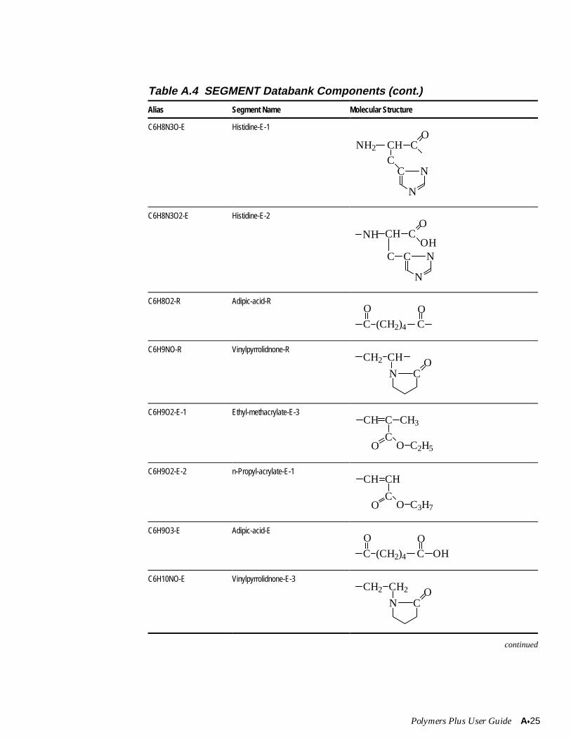
Polymers Plus User Guide Ax25
Table A.4 SEGMENT Databank Components (cont.)
Alias Segment Name Molecular Structure
C6H8N3O-E Histidine-E-1
NH2 CH CC
O
NC
N
C6H8N3O2-E Histidine-E-2
CH CO
NHOH
NC
N
C
C6H8O2-R Adipic-acid-R
CC (CH2)4
O O
C6H9NO-R Vinylpyrrolidnone-RCH2 CH
CNO
C6H9O2-E-1 Ethyl-methacrylate-E-3CH C CH3
CO C2H5O
C6H9O2-E-2 n-Propyl-acrylate-E-1CH CH
CO C3H7O
C6H9O3-E Adipic-acid-E
C OHC (CH2)4
O O
C6H10NO-E Vinylpyrrolidnone-E-3CH2 CH2
N CO
continued
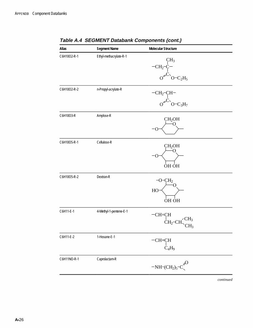
APPENDIX Component Databanks
Ax26
Table A.4 SEGMENT Databank Components (cont.)
Alias Segment Name Molecular Structure
C6H10O2-R-1 Ethyl-methacrylate-R-1
CH2 C
CO C2H5O
CH3
C6H10O2-R-2 n-Propyl-acrylate-RCH2 CH
CO C3H7O
C6H10O3-R Amylose-R
OCH2OH
O
C6H10O5-R-1 Cellulose-R
OCH2OH
O
OH OH
C6H10O5-R-2 Dextran-R
O
OH OH
HO
CH2O
C6H11-E-1 4-Methyl-1-pentene-E-1CH CH
CH2 CHCH3
CH3
C6H11-E-2 1-Hexane-E-1CH CH
C4H9
C6H11NO-R-1 Caprolactam-R
NH (CH2)5 CO
continued
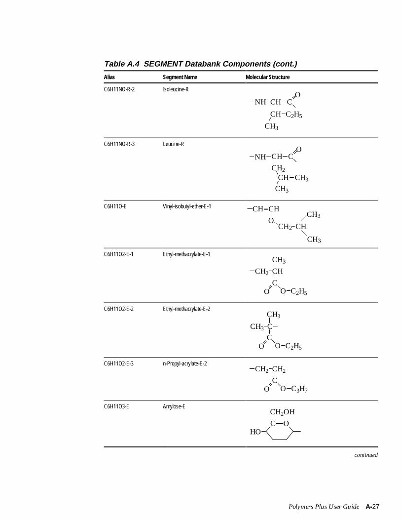
Polymers Plus User Guide Ax27
Table A.4 SEGMENT Databank Components (cont.)
Alias Segment Name Molecular Structure
C6H11NO-R-2 Isoleucine-R
NH CH
CH C2H5
OC
CH3
C6H11NO-R-3 Leucine-RO
C
CH3
CH
CH2
NH
CH
CH3
C6H11O-E Vinyl-isobutyl-ether-E-1
CH3
CH CH
OCH2 CH
CH3
C6H11O2-E-1 Ethyl-methacrylate-E-1
CH2 CH
CH3
CO O C2H5
C6H11O2-E-2 Ethyl-methacrylate-E-2
O O C2H5
C
CH3
CCH3
C6H11O2-E-3 n-Propyl-acrylate-E-2
O O C3H7
C
CH2 CH2
C6H11O3-E Amylose-E
C O
CH2OH
HO
continued
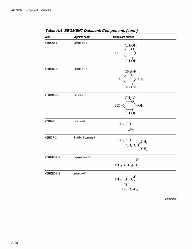
APPENDIX Component Databanks
Ax28
Table A.4 SEGMENT Databank Components (cont.)
Alias Segment Name Molecular Structure
C6H11O5-E Cellulose-E-1
OCH2OH
HO
OH OH
C6H11O6-E-1 Cellulose-E-2
OCH2OH
OH
OH OH
O
C6H11O6-E-2 Dextran-E-2
OOH
OH OH
CH2 O
HO
C6H12-R-1 1-Hexane-RCH2 CH
C4H9
C6H12-R-2 4-Methyl-1-pentene-RCH2 CH
CH2 CHCH3
CH3
C6H12NO-E-1 Caprolactam-E-1
NH2 (CH2)5 C
O
C6H12NO-E-2 Isoleucine-E-1
NH2 CH C
CH
O
CH3 C2H5
continued
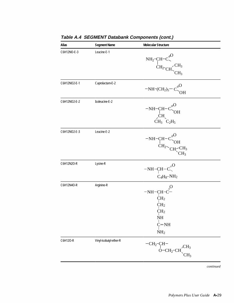
Polymers Plus User Guide Ax29
Table A.4 SEGMENT Databank Components (cont.)
Alias Segment Name Molecular Structure
C6H12NO-E-3 Leucine-E-1
NH2 CH C
CH2 CH
O
CH3
CH3
C6H12NO2-E-1 Caprolactam-E-2 OC
OH(CH2)5NH
C6H12NO2-E-2 Isoleucine-E-2O
COH
NH CH
CHC2H5CH3
C6H12NO2-E-3 Leucine-E-2O
COH
NH CH
CH2
CH3
CH CH3
C6H12N2O-R Lysine-R OCNH CH
C4H8 NH2
C6H12N4O-R Arginine-R
NH CH CCH2
CH2
CH2
NH
C NH
NH2
O
C6H12O-R Vinyl-isobutyl-ether-RCH2 CH
O CH2 CHCH3
CH3
continued
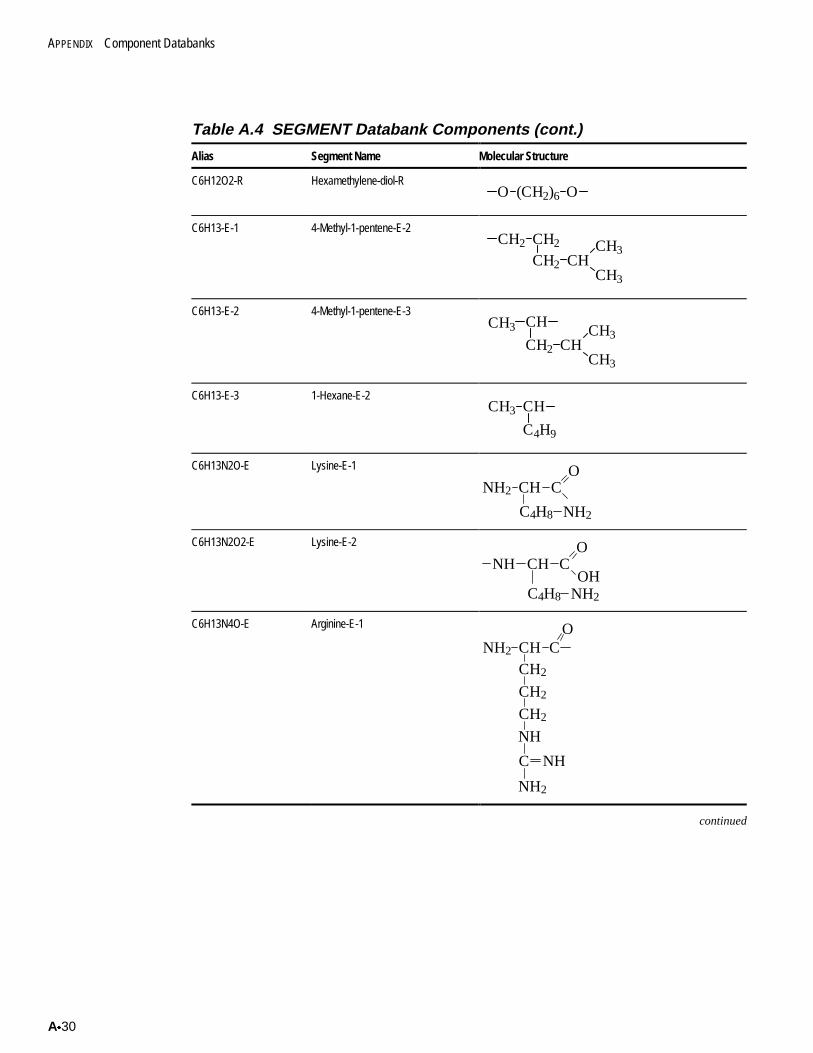
APPENDIX Component Databanks
Ax30
Table A.4 SEGMENT Databank Components (cont.)
Alias Segment Name Molecular Structure
C6H12O2-R Hexamethylene-diol-RO (CH2)6 O
C6H13-E-1 4-Methyl-1-pentene-E-2CH2 CH2
CH2 CHCH3
CH3
C6H13-E-2 4-Methyl-1-pentene-E-3
CH3
CH3
CH2 CH
CHCH3
C6H13-E-3 1-Hexane-E-2CH3 CH
C4H9
C6H13N2O-E Lysine-E-1
NH2 CH CO
NH2C4H8
C6H13N2O2-E Lysine-E-2 OCH CNH
OHNH2C4H8
C6H13N4O-E Arginine-E-1 OCH CCH2
CH2
CH2
NH
C NH
NH2
NH2
continued
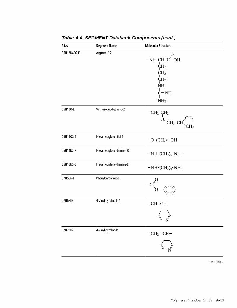
Polymers Plus User Guide Ax31
Table A.4 SEGMENT Databank Components (cont.)
Alias Segment Name Molecular Structure
C6H13N4O2-E Arginine-E-2
CH CCH2
CH2
CH2
NH
C NH
NH2
NHO
OH
C6H13O-E Vinyl-isobutyl-ether-E-2CH2 CH2
OCH2 CH
CH3
CH3
C6H13O2-E Hexamethylene-diol-EO (CH2)6 OH
C6H14N2-R Hexamethylene-diamine-R(CH2)6 NHNH
C6H15N2-E Hexamethylene-diamine-E(CH2)6NH NH2
C7H5O2-E Phenylcarbonate-E
CO
O
C7H6N-E 4-Vinyl-pyridine-E-1CH CH
N
C7H7N-R 4-Vinyl-pyridine-R
N
CHCH2
continued
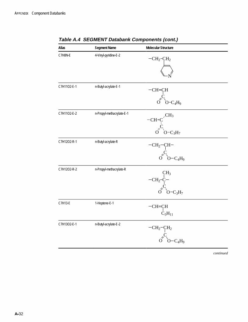
APPENDIX Component Databanks
Ax32
Table A.4 SEGMENT Databank Components (cont.)
Alias Segment Name Molecular Structure
C7H8N-E 4-Vinyl-pyridine-E-2
N
CH2 CH2
C7H11O2-E-1 n-Butyl-acrylate-E-1CH CH
CO O C4H9
C7H11O2-E-2 n-Propyl-methacrylate-E-1
CH CC
O O C3H7
CH3
C7H12O2-R-1 n-Butyl-acrylate-RCH
O O C4H9
C
CH2
C7H12O2-R-2 n-Propyl-methacrylate-R
O O C3H7
CH2 CC
CH3
C7H13-E 1-Heptene-E-1CH CH
C5H11
C7H13O2-E-1 n-Butyl-acrylate-E-2
O O C4H9
CH2 CH2
C
continued
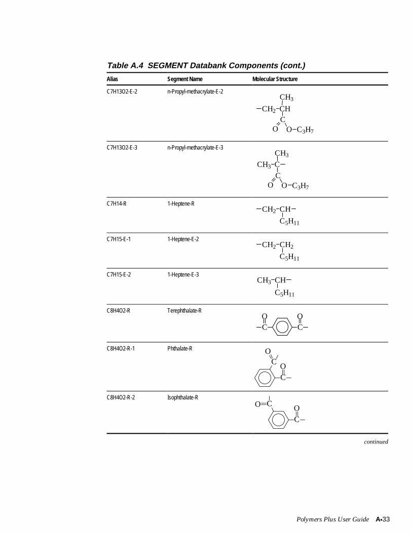
Polymers Plus User Guide Ax33
Table A.4 SEGMENT Databank Components (cont.)
Alias Segment Name Molecular Structure
C7H13O2-E-2 n-Propyl-methacrylate-E-2
O O C3H7
CH2 CHC
CH3
C7H13O2-E-3 n-Propyl-methacrylate-E-3
O O C3H7
CH3
C
CH3 C
C7H14-R 1-Heptene-RCH2 CH
C5H11
C7H15-E-1 1-Heptene-E-2CH2 CH2
C5H11
C7H15-E-2 1-Heptene-E-3
C5H11
CH3 CH
C8H4O2-R Terephthalate-R
C CO O
C8H4O2-R-1 Phthalate-R
C
C
O
O
C8H4O2-R-2 Isophthalate-RC
COO
continued
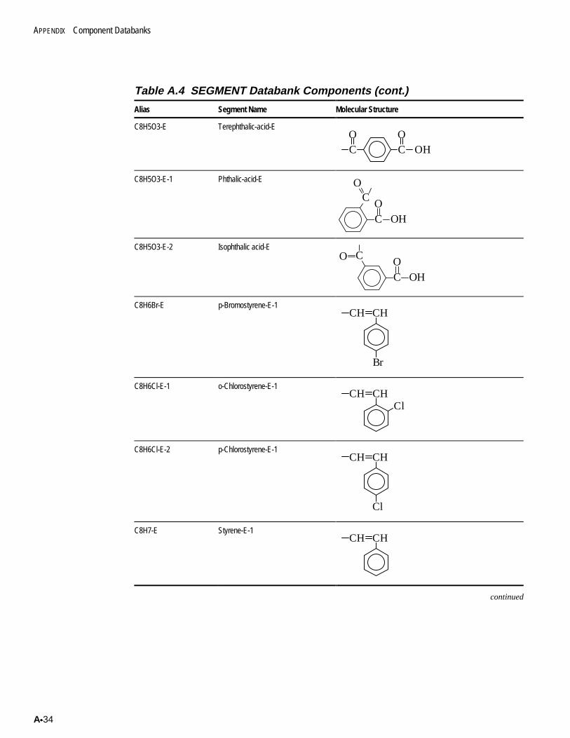
APPENDIX Component Databanks
Ax34
Table A.4 SEGMENT Databank Components (cont.)
Alias Segment Name Molecular Structure
C8H5O3-E Terephthalic-acid-E
C CO O
OH
C8H5O3-E-1 Phthalic-acid-E
C
C OH
O
O
C8H5O3-E-2 Isophthalic acid-EC
COO
OH
C8H6Br-E p-Bromostyrene-E-1
Br
CHCH
C8H6Cl-E-1 o-Chlorostyrene-E-1CHCH
Cl
C8H6Cl-E-2 p-Chlorostyrene-E-1CHCH
Cl
C8H7-E Styrene-E-1CHCH
continued
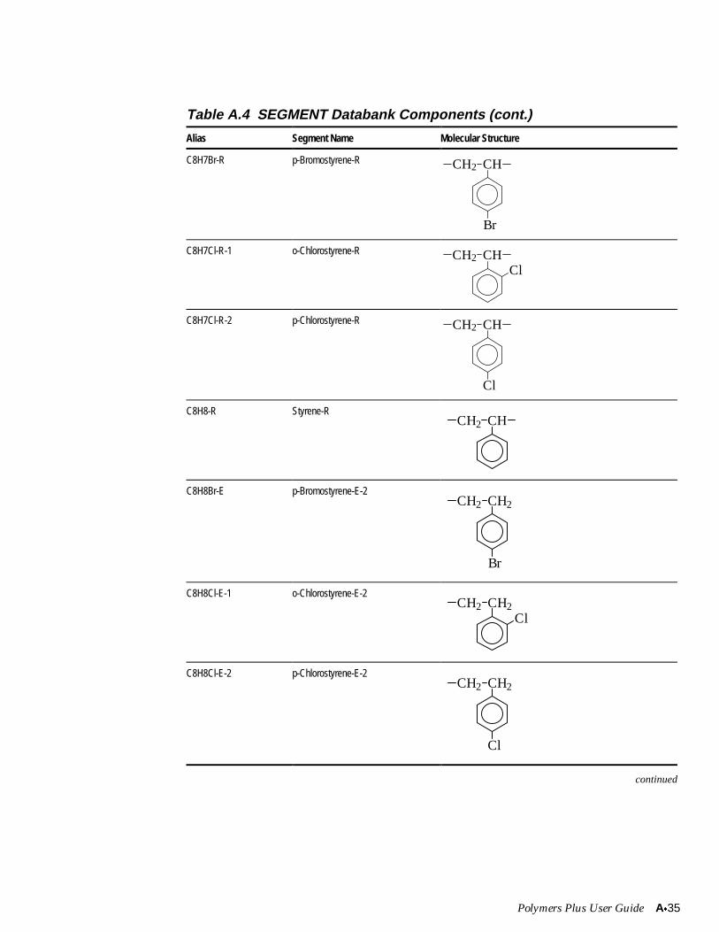
Polymers Plus User Guide Ax35
Table A.4 SEGMENT Databank Components (cont.)
Alias Segment Name Molecular Structure
C8H7Br-R p-Bromostyrene-R CH
Br
CH2
C8H7Cl-R-1 o-Chlorostyrene-R CHCl
CH2
C8H7Cl-R-2 p-Chlorostyrene-R CH
Cl
CH2
C8H8-R Styrene-RCHCH2
C8H8Br-E p-Bromostyrene-E-2CH2 CH2
Br
C8H8Cl-E-1 o-Chlorostyrene-E-2CH2 CH2
Cl
C8H8Cl-E-2 p-Chlorostyrene-E-2CH2 CH2
Cl
continued
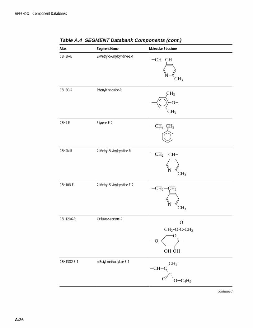
APPENDIX Component Databanks
Ax36
Table A.4 SEGMENT Databank Components (cont.)
Alias Segment Name Molecular Structure
C8H8N-E 2-Methyl-5-vinylpyridine-E-1CH CH
NCH3
C8H8O-R Phenylene-oxide-R
CH3
CH3
O
C8H9-E Styrene-E-2CH2 CH2
C8H9N-R 2-Methyl-5-vinylpyridine-R
NCH3
CHCH2
C8H10N-E 2-Methyl-5-vinylpyridine-E-2CH2 CH2
CH3N
C8H12O6-R Cellulose-acetate-R
O
OH OH
O
CH2 O C CH3
O
C8H13O2-E-1 n-Butyl-methacrylate-E-1
CH CCH3
CO O C4H9
continued
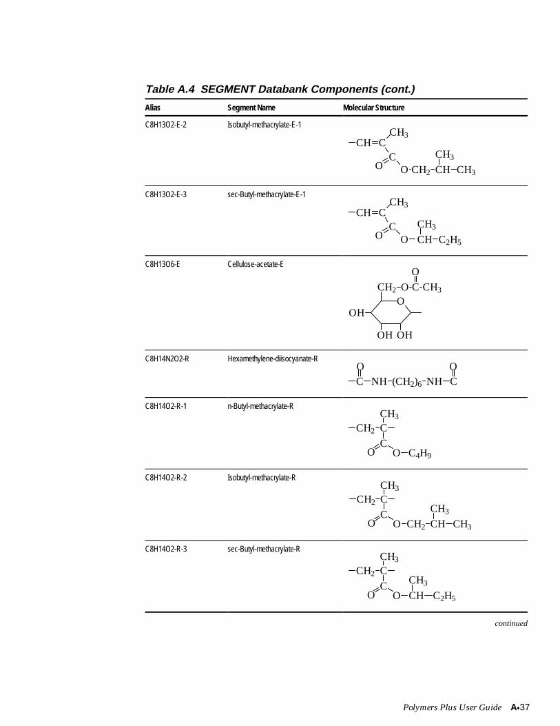
Polymers Plus User Guide Ax37
Table A.4 SEGMENT Databank Components (cont.)
Alias Segment Name Molecular Structure
C8H13O2-E-2 Isobutyl-methacrylate-E-1
CH CCH3
CO O CH2 CH CH3
CH3
C8H13O2-E-3 sec-Butyl-methacrylate-E-1
CH CCH3
CO O CH
CH3
C2H5
C8H13O6-E Cellulose-acetate-E
O
OH OH
CH2 O C CH3
O
OH
C8H14N2O2-R Hexamethylene-diisocyanate-R
C NH (CH2)6 NH CO O
C8H14O2-R-1 n-Butyl-methacrylate-R
CH2 CCH3
CO O C4H9
C8H14O2-R-2 Isobutyl-methacrylate-R
CH2 CCH3
CO O CH2 CH CH3
CH3
C8H14O2-R-3 sec-Butyl-methacrylate-R
CH2 CCH3
CO O CH
CH3
C2H5
continued
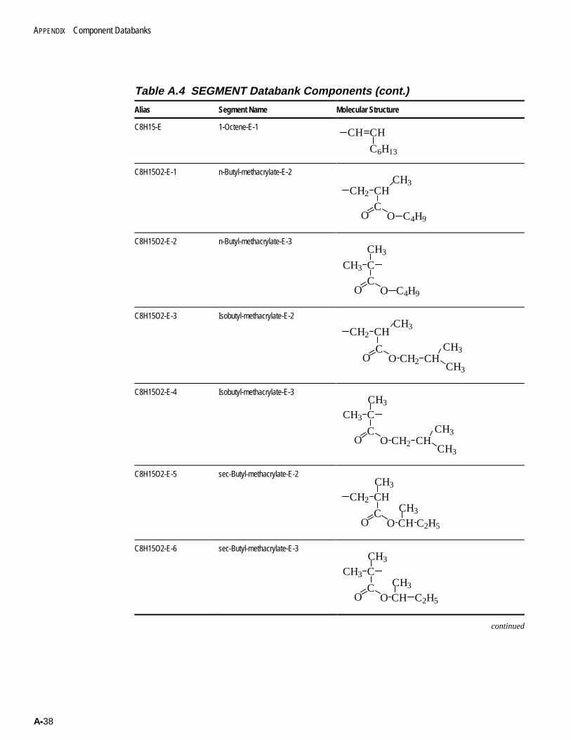
APPENDIX Component Databanks
Ax38
Table A.4 SEGMENT Databank Components (cont.)
Alias Segment Name Molecular Structure
C8H15-E 1-Octene-E-1CH CH
C6H13
C8H15O2-E-1 n-Butyl-methacrylate-E-2
CH2 CH
CO O C4H9
CH3
C8H15O2-E-2 n-Butyl-methacrylate-E-3
O O C4H9
C
CCH3
CH3
C8H15O2-E-3 Isobutyl-methacrylate-E-2
O O CH2 CHC
CH3CH2 CH
CH3
CH3
C8H15O2-E-4 Isobutyl-methacrylate-E-3
O O CH2 CHC
CH3
CH3
CH3
CH3 C
C8H15O2-E-5 sec-Butyl-methacrylate-E-2
O O CH C2H5
C
CH3
CH3
CH2 CH
C8H15O2-E-6 sec-Butyl-methacrylate-E-3
O O CHC
CH3
CH3
CH3 C
C2H5
continued
Polymers Plus User Guide Ax39
Table A.4 SEGMENT Databank Components (cont.)
Alias Segment Name Molecular Structure
C8H16-R 1-Octene-RCH2 CH
C6H13
C8H17-E-1 1-Octene-E-2CH2 CH2
C6H13
C8H17-E-2 1-Octene-E-3
C6H13
CH3 CH
C9H7O3-E dimethyl-terephthalate-E
C CO O
CH3O
C9H9-E-1 alpha-Methylstyrene-E-1
CCH
CH3
C9H9-E-2 m-Methylstyrene-E-1
CH3
CHCH
C9H9-E-3 o-Methylstyrene-E-1CHCH
CH3
C9H9-E-4 p-Methylstyrene-E-1CHCH
CH3
continued
APPENDIX Component Databanks
Ax40
Table A.4 SEGMENT Databank Components (cont.)
Alias Segment Name Molecular Structure
C9H9NO-R Phenylalanine-R
CH2
CH CNHO
C9H9NO2-R Tyrosine-R
CH2
CH C
OH
NHO
C9H9O-E p-Methoxystyrene-E-1
OCH3
CHCH
C9H10-R-1 alpha-Methylstyrene-R
CCH2
CH3
C9H10-R-2 m-Methylstyrene-R
CH3
CHCH2
C9H10-R-3 o-Methylstyrene-RCH
CH3
CH2
continued
Polymers Plus User Guide Ax41
Table A.4 SEGMENT Databank Components (cont.)
Alias Segment Name Molecular Structure
C9H10-R-4 p-Methylstyrene-RCH
CH3
CH2
C9H10NO-E Phenylalanine-E-1
CH2
CH CNH2
O
C9H10NO2-E-1 Phenylalanine-E-2
CH2
CH CNHO
OH
C9H10NO2-E-2 Tyrosine-E-1
CH2
CH CNH2
OH
O
C9H10NO3-E Tyrosine-E-2
CH2
CH C
OH
NHO
OH
continued
APPENDIX Component Databanks
Ax42
Table A.4 SEGMENT Databank Components (cont.)
Alias Segment Name Molecular Structure
C9H10O-R p-Methoxystyrene-RCH
OCH3
CH2
C9H11-E-1 alpha-Methylstyrene-E-2
CH
CH3
CH2
C9H11-E-2 alpha-Methylstyrene-E-3CH3
CH3 C
C9H11-E-3 m-Methylstyrene-E-2
CH3
CH2 CH2
C9H11-E-4 o-Methylstyrene-E-2
CH3
CH2 CH2
C9H11-E-5 p-Methylstyrene-E-2
CH3
CH2 CH2
continued
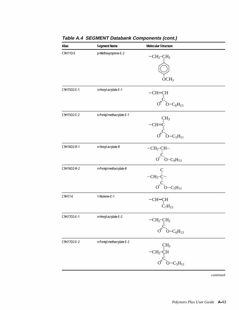
Polymers Plus User Guide Ax43
Table A.4 SEGMENT Databank Components (cont.)
Alias Segment Name Molecular Structure
C9H11O-E p-Methoxystyrene-E-2
OCH3
CH2 CH2
C9H15O2-E-1 n-Hexyl-acrylate-E-1CH CH
CO O C6H13
C9H15O2-E-2 n-Pentyl-methacrylate-E-1
CH C
C
CH3
O O C5H11
C9H16O2-R-1 n-Hexyl-acrylate-R
O O C6H13
CH
C
CH2
C9H16O2-R-2 n-Pentyl-methacrylate-R
O O C5H11
CCH2 C
C
C9H17-E 1-Nonene-E-1CH CH
C7H15
C9H17O2-E-1 n-Hexyl-acrylate-E-2
O O C6H13
CH2 CH2
C
C9H17O2-E-2 n-Pentyl-methacrylate-E-2
O O C5H11
CH3
CHCH2
C
continued
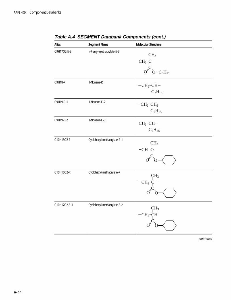
APPENDIX Component Databanks
Ax44
Table A.4 SEGMENT Databank Components (cont.)
Alias Segment Name Molecular Structure
C9H17O2-E-3 n-Pentyl-methacrylate-E-3
O O C5H11
C
CH3
CCH3
C9H18-R 1-Nonene-RCH2 CH
C7H15
C9H19-E-1 1-Nonene-E-2CH2 CH2
C7H15
C9H19-E-2 1-Nonene-E-3CH
C7H15
CH3
C10H15O2-E Cyclohexyl-methacrylate-E-1
O OC
CH3
CCH
C10H16O2-R Cyclohexyl-methacrylate-R
O OC
CH3
CCH2
C10H17O2-E-1 Cyclohexyl-methacrylate-E-2
O OC
CH3
CHCH2
continued
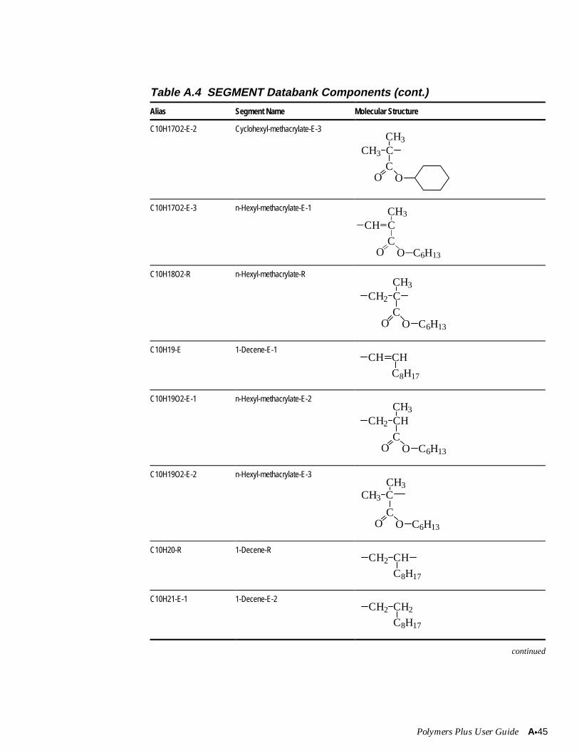
Polymers Plus User Guide Ax45
Table A.4 SEGMENT Databank Components (cont.)
Alias Segment Name Molecular Structure
C10H17O2-E-2 Cyclohexyl-methacrylate-E-3
O OC
CH3
CCH3
C10H17O2-E-3 n-Hexyl-methacrylate-E-1
O OC
C6H13
CH3
CCH
C10H18O2-R n-Hexyl-methacrylate-R
O OC
C6H13
CH3
CCH2
C10H19-E 1-Decene-E-1CH CH
C8H17
C10H19O2-E-1 n-Hexyl-methacrylate-E-2
O OC
C6H13
CH3
CHCH2
C10H19O2-E-2 n-Hexyl-methacrylate-E-3
O OC
C6H13
CH3CCH3
C10H20-R 1-Decene-RCH
C8H17
CH2
C10H21-E-1 1-Decene-E-2CH2 CH2
C8H17
continued
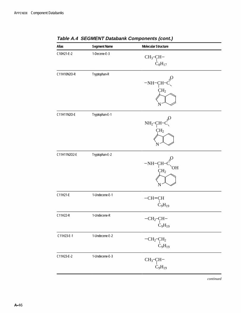
APPENDIX Component Databanks
Ax46
Table A.4 SEGMENT Databank Components (cont.)
Alias Segment Name Molecular Structure
C10H21-E-2 1-Decene-E-3CH3 CH
C8H17
C11H10N2O-R Tryptophan-R
NH CH C
CH2
N
O
C11H11N2O-E Tryptophan-E-1
CH2
N
CH CNH2
O
C11H11N2O2-E Tryptophan-E-2
NH CH C
CH2
N
O
OH
C11H21-E 1-Undecene-E-1CH CH
C9H19
C11H22-R 1-Undecene-RCH
C9H19
CH2
C11H23-E-1 1-Undecene-E-2CH2 CH2
C9H19
C11H23-E-2 1-Undecene-E-3CH3 CH
C9H19
continued
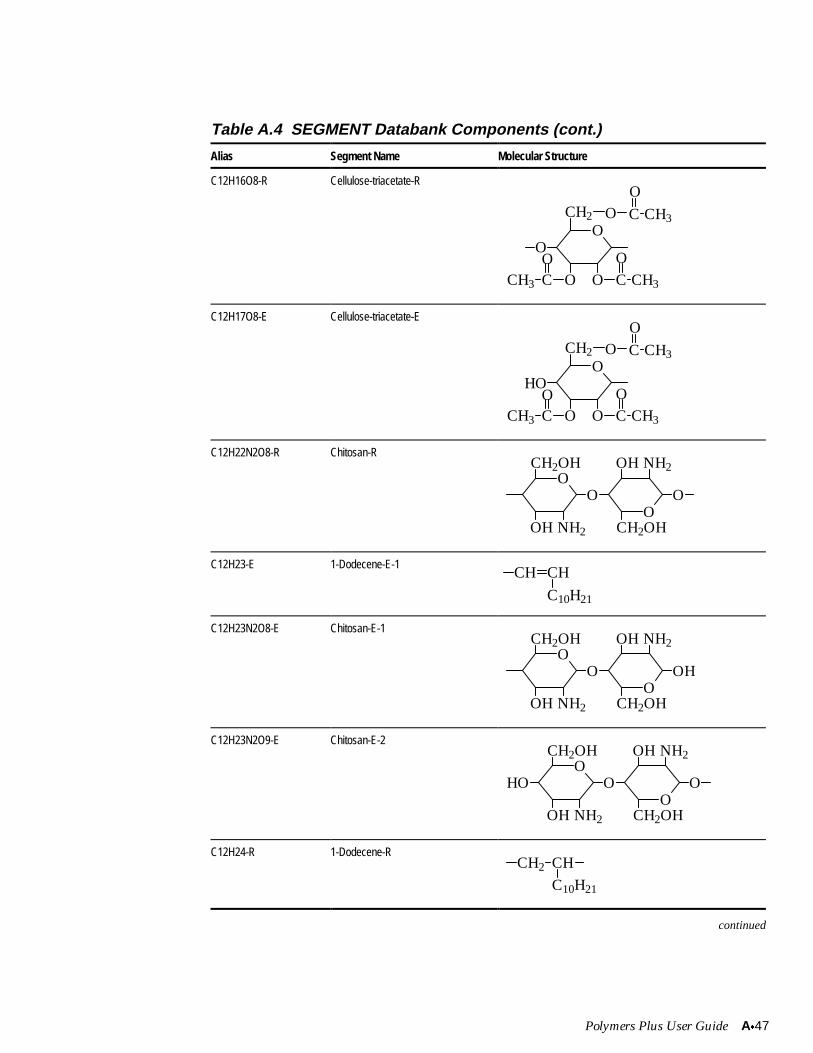
Polymers Plus User Guide Ax47
Table A.4 SEGMENT Databank Components (cont.)
Alias Segment Name Molecular Structure
C12H16O8-R Cellulose-triacetate-R
O
O O
O
CCCH3 CH3
CH2
OO
O C CH3
O
C12H17O8-E Cellulose-triacetate-E
O
O O CCCH3 CH3
CH2
HOOO
O C CH3
O
C12H22N2O8-R Chitosan-R
OO
OH NH2
CH2OH
OCH2OH
O
NH2OH
C12H23-E 1-Dodecene-E-1CH CH
C10H21
C12H23N2O8-E Chitosan-E-1
OO
OH NH2
CH2OH
OCH2OH
NH2OH
OH
C12H23N2O9-E Chitosan-E-2
OO
OH NH2
CH2OH
HOO
CH2OH
NH2OH
O
C12H24-R 1-Dodecene-RCH2 CH
C10H21
continued
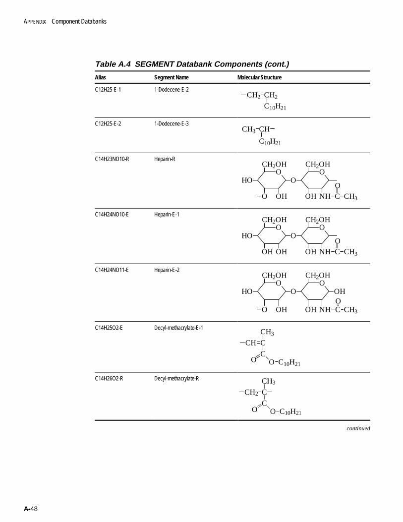
APPENDIX Component Databanks
Ax48
Table A.4 SEGMENT Databank Components (cont.)
Alias Segment Name Molecular Structure
C12H25-E-1 1-Dodecene-E-2CH2 CH2
C10H21
C12H25-E-2 1-Dodecene-E-3
C10H21
CH3 CH
C14H23NO10-R Heparin-R
OO
O OH
CH2OH
HOO
OH NH C CH3
CH2OH
O
C14H24NO10-E Heparin-E-1
OO
OH
CH2OH
HO
OH
O
OH NH C CH3
CH2OH
O
C14H24NO11-E Heparin-E-2
OO
OH
CH2OH
HO
O
O
OH NH
OH
CH2OH
C CH3
O
C14H25O2-E Decyl-methacrylate-E-1
CH C
CH3
CO C10H21
O
C14H26O2-R Decyl-methacrylate-R
O C10H21O
C
CH3
C
CH2
continued
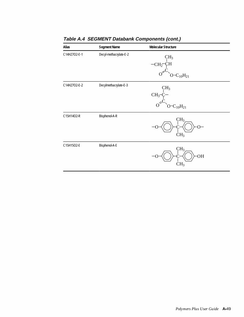
Polymers Plus User Guide Ax49
Table A.4 SEGMENT Databank Components (cont.)
Alias Segment Name Molecular Structure
C14H27O2-E-1 Decyl-methacrylate-E-2
CH
CH3
O C10H21
CCH2
O
C14H27O2-E-2 Decylmethacrylate-E-3
O C10H21
C
CH3
CH3 C
O
C15H14O2-R Bisphenol-A-R
O C
CH3
CH3
O
C15H15O2-E Bisphenol-A-E
O C
CH3
CH3
OH

APPENDIX Component Databanks
Ax50
Polymers Plus User Guide Bx1
B PHYSICAL PROPERTY METHODS
This appendix documents the physical property route structure for the polymer specificproperty methods:
x POLYFH - Flory-Huggins property method (Bx2)x POLYNRTL - Non-random two liquid property method (Bx4)x POLYUF - UNIFAC property method (Bx6)x POLYUFV - UNIFAC free volume property method (Bx8)x POLYSL - Sanchez-Lacombe EOS property method (Bx10)x POLSRK - Polymer Soave-Redlich-Kwong EOS Property Method (Bx12)x POLYSAFT - SAFT EOS Property Method (Bx14)
For each property method the property models used in the route calculations aredescribed.
B
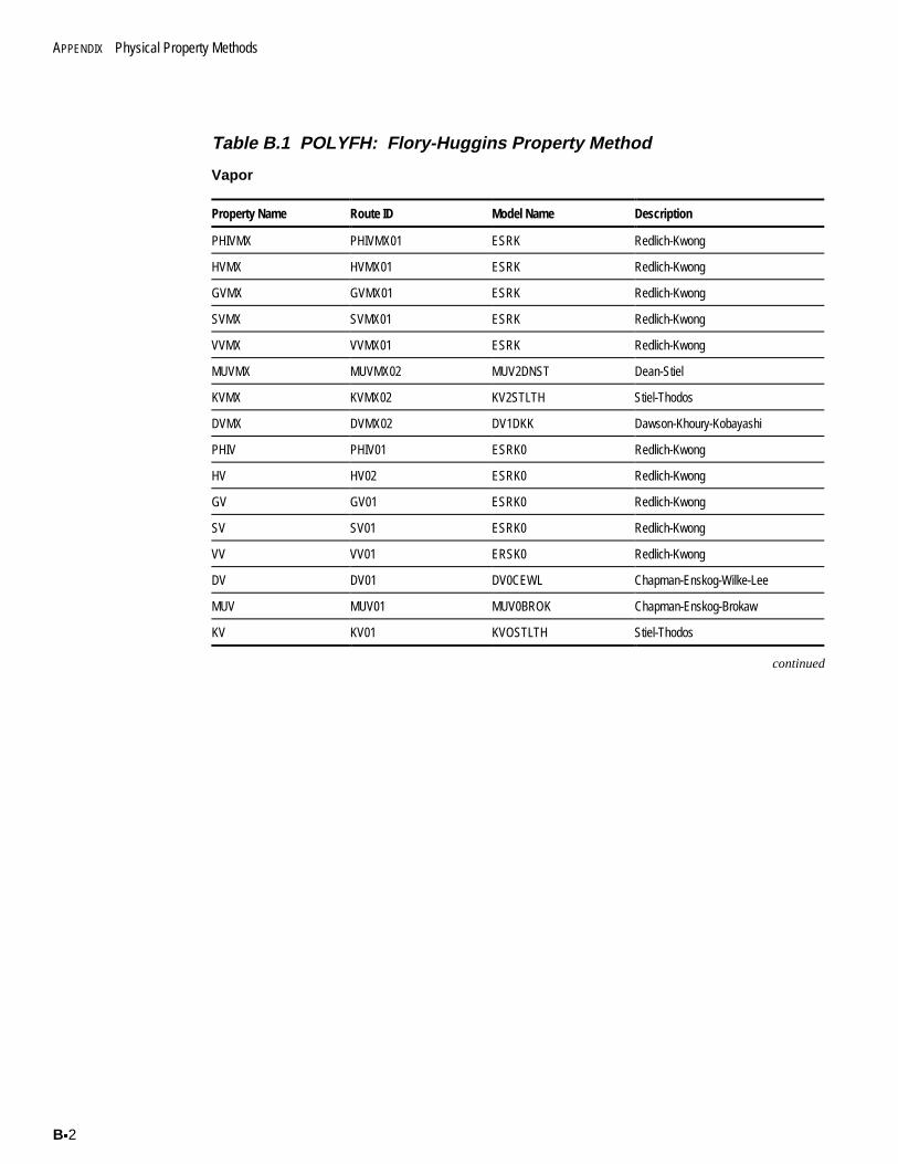
APPENDIX Physical Property Methods
Bx2
Table B.1 POLYFH: Flory-Huggins Property Method
Vapor
Property Name Route ID Model Name Description
PHIVMX PHIVMX01 ESRK Redlich-Kwong
HVMX HVMX01 ESRK Redlich-Kwong
GVMX GVMX01 ESRK Redlich-Kwong
SVMX SVMX01 ESRK Redlich-Kwong
VVMX VVMX01 ESRK Redlich-Kwong
MUVMX MUVMX02 MUV2DNST Dean-Stiel
KVMX KVMX02 KV2STLTH Stiel-Thodos
DVMX DVMX02 DV1DKK Dawson-Khoury-Kobayashi
PHIV PHIV01 ESRK0 Redlich-Kwong
HV HV02 ESRK0 Redlich-Kwong
GV GV01 ESRK0 Redlich-Kwong
SV SV01 ESRK0 Redlich-Kwong
VV VV01 ERSK0 Redlich-Kwong
DV DV01 DV0CEWL Chapman-Enskog-Wilke-Lee
MUV MUV01 MUV0BROK Chapman-Enskog-Brokaw
KV KV01 KVOSTLTH Stiel-Thodos
continued
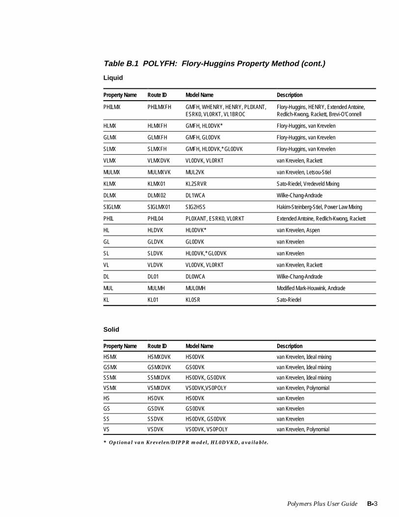
Polymers Plus User Guide Bx3
Table B.1 POLYFH: Flory-Huggins Property Method (cont.)
Liquid
Property Name Route ID Model Name Description
PHILMX PHILMXFH GMFH, WHENRY, HENRY, PL0XANT,ESRK0, VL0RKT, VL1BROC
Flory-Huggins, HENRY, Extended Antoine,Redlich-Kwong, Rackett, Brevi-O'Connell
HLMX HLMXFH GMFH, HL0DVK* Flory-Huggins, van Krevelen
GLMX GLMXFH GMFH, GL0DVK Flory-Huggins, van Krevelen
SLMX SLMXFH GMFH, HL0DVK,* GL0DVK Flory-Huggins, van Krevelen
VLMX VLMXDVK VL0DVK, VL0RKT van Krevelen, Rackett
MULMX MULMXVK MUL2VK van Krevelen, Letsou-Stiel
KLMX KLMX01 KL2SRVR Sato-Riedel, Vredeveld Mixing
DLMX DLMX02 DL1WCA Wilke-Chang-Andrade
SIGLMX SIGLMX01 SIG2HSS Hakim-Steinberg-Stiel, Power Law Mixing
PHIL PHIL04 PL0XANT, ESRK0, VL0RKT Extended Antoine, Redlich-Kwong, Rackett
HL HLDVK HL0DVK* van Krevelen, Aspen
GL GLDVK GL0DVK van Krevelen
SL SLDVK HL0DVK,* GL0DVK van Krevelen
VL VLDVK VL0DVK, VL0RKT van Krevelen, Rackett
DL DL01 DL0WCA Wilke-Chang-Andrade
MUL MULMH MUL0MH Modified Mark-Houwink, Andrade
KL KL01 KL0SR Sato-Riedel
Solid
Property Name Route ID Model Name Description
HSMX HSMXDVK HS0DVK van Krevelen, Ideal mixing
GSMX GSMXDVK GS0DVK van Krevelen, Ideal mixing
SSMX SSMXDVK HS0DVK, GS0DVK van Krevelen, Ideal mixing
VSMX VSMXDVK VS0DVK,VS0POLY van Krevelen, Polynomial
HS HSDVK HS0DVK van Krevelen
GS GSDVK GS0DVK van Krevelen
SS SSDVK HS0DVK, GS0DVK van Krevelen
VS VSDVK VS0DVK, VS0POLY van Krevelen, Polynomial
* Optional van Krevelen/DIPPR model, HL0DVKD, available.
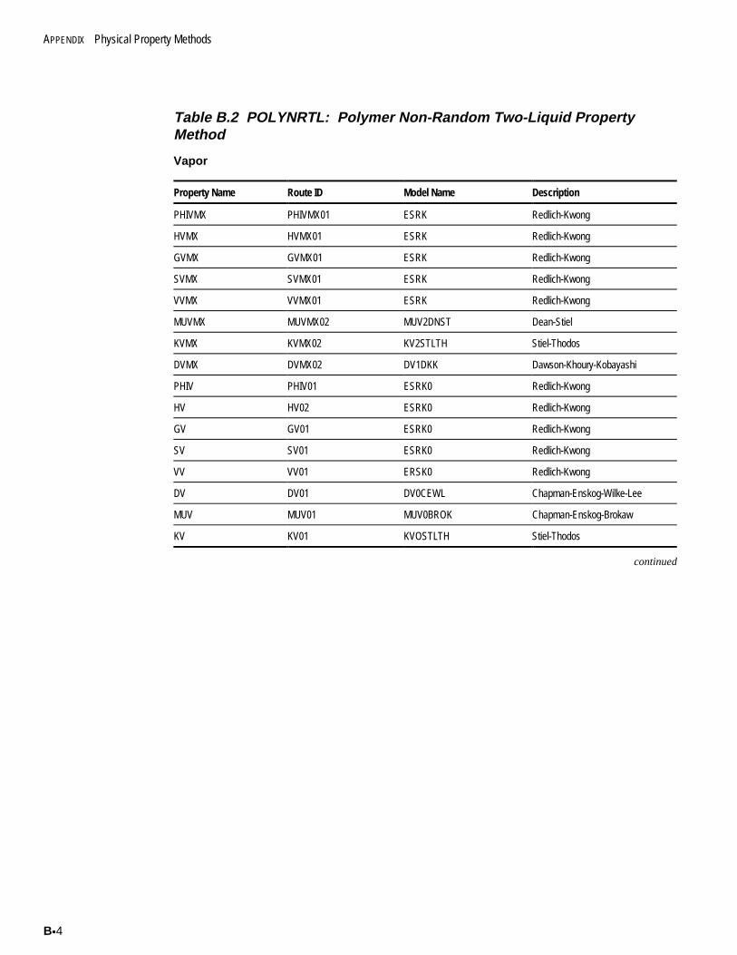
APPENDIX Physical Property Methods
Bx4
Table B.2 POLYNRTL: Polymer Non-Random Two-Liquid PropertyMethod
Vapor
Property Name Route ID Model Name Description
PHIVMX PHIVMX01 ESRK Redlich-Kwong
HVMX HVMX01 ESRK Redlich-Kwong
GVMX GVMX01 ESRK Redlich-Kwong
SVMX SVMX01 ESRK Redlich-Kwong
VVMX VVMX01 ESRK Redlich-Kwong
MUVMX MUVMX02 MUV2DNST Dean-Stiel
KVMX KVMX02 KV2STLTH Stiel-Thodos
DVMX DVMX02 DV1DKK Dawson-Khoury-Kobayashi
PHIV PHIV01 ESRK0 Redlich-Kwong
HV HV02 ESRK0 Redlich-Kwong
GV GV01 ESRK0 Redlich-Kwong
SV SV01 ESRK0 Redlich-Kwong
VV VV01 ERSK0 Redlich-Kwong
DV DV01 DV0CEWL Chapman-Enskog-Wilke-Lee
MUV MUV01 MUV0BROK Chapman-Enskog-Brokaw
KV KV01 KVOSTLTH Stiel-Thodos
continued
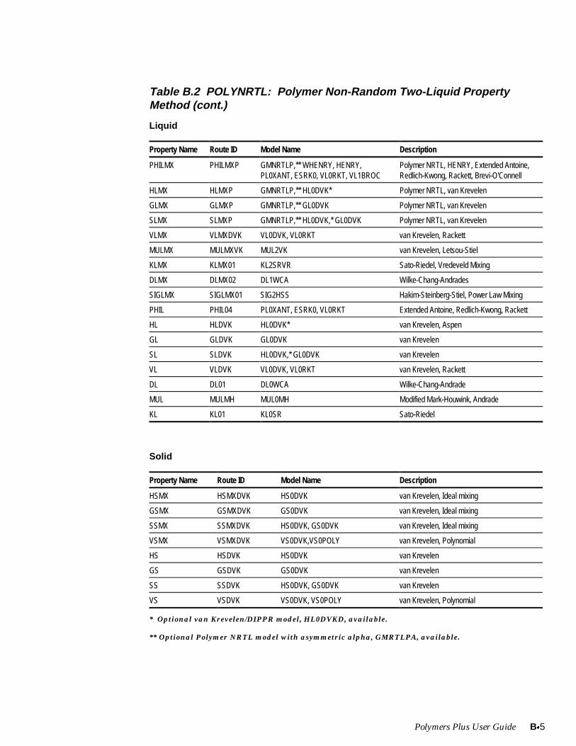
Polymers Plus User Guide Bx5
Table B.2 POLYNRTL: Polymer Non-Random Two-Liquid PropertyMethod (cont.)
Liquid
Property Name Route ID Model Name Description
PHILMX PHILMXP GMNRTLP,** WHENRY, HENRY,PL0XANT, ESRK0, VL0RKT, VL1BROC
Polymer NRTL, HENRY, Extended Antoine,Redlich-Kwong, Rackett, Brevi-O'Connell
HLMX HLMXP GMNRTLP,** HL0DVK* Polymer NRTL, van Krevelen
GLMX GLMXP GMNRTLP,** GL0DVK Polymer NRTL, van Krevelen
SLMX SLMXP GMNRTLP,** HL0DVK,* GL0DVK Polymer NRTL, van Krevelen
VLMX VLMXDVK VL0DVK, VL0RKT van Krevelen, Rackett
MULMX MULMXVK MUL2VK van Krevelen, Letsou-Stiel
KLMX KLMX01 KL2SRVR Sato-Riedel, Vredeveld Mixing
DLMX DLMX02 DL1WCA Wilke-Chang-Andrades
SIGLMX SIGLMX01 SIG2HSS Hakim-Steinberg-Stiel, Power Law Mixing
PHIL PHIL04 PL0XANT, ESRK0, VL0RKT Extended Antoine, Redlich-Kwong, Rackett
HL HLDVK HL0DVK* van Krevelen, Aspen
GL GLDVK GL0DVK van Krevelen
SL SLDVK HL0DVK,* GL0DVK van Krevelen
VL VLDVK VL0DVK, VL0RKT van Krevelen, Rackett
DL DL01 DL0WCA Wilke-Chang-Andrade
MUL MULMH MUL0MH Modified Mark-Houwink, Andrade
KL KL01 KL0SR Sato-Riedel
Solid
Property Name Route ID Model Name Description
HSMX HSMXDVK HS0DVK van Krevelen, Ideal mixing
GSMX GSMXDVK GS0DVK van Krevelen, Ideal mixing
SSMX SSMXDVK HS0DVK, GS0DVK van Krevelen, Ideal mixing
VSMX VSMXDVK VS0DVK,VS0POLY van Krevelen, Polynomial
HS HSDVK HS0DVK van Krevelen
GS GSDVK GS0DVK van Krevelen
SS SSDVK HS0DVK, GS0DVK van Krevelen
VS VSDVK VS0DVK, VS0POLY van Krevelen, Polynomial
* Optional van Krevelen/DIPPR model, HL0DVKD, available.
** Optional Polymer NRTL model with asymmetric alpha, GMRTLPA, available.
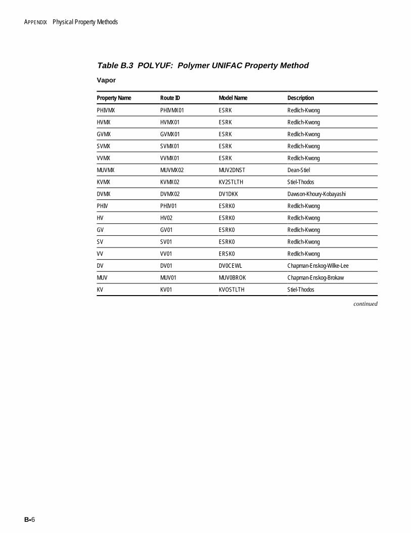
APPENDIX Physical Property Methods
Bx6
Table B.3 POLYUF: Polymer UNIFAC Property Method
Vapor
Property Name Route ID Model Name Description
PHIVMX PHIVMX01 ESRK Redlich-Kwong
HVMX HVMX01 ESRK Redlich-Kwong
GVMX GVMX01 ESRK Redlich-Kwong
SVMX SVMX01 ESRK Redlich-Kwong
VVMX VVMX01 ESRK Redlich-Kwong
MUVMX MUVMX02 MUV2DNST Dean-Stiel
KVMX KVMX02 KV2STLTH Stiel-Thodos
DVMX DVMX02 DV1DKK Dawson-Khoury-Kobayashi
PHIV PHIV01 ESRK0 Redlich-Kwong
HV HV02 ESRK0 Redlich-Kwong
GV GV01 ESRK0 Redlich-Kwong
SV SV01 ESRK0 Redlich-Kwong
VV VV01 ERSK0 Redlich-Kwong
DV DV01 DV0CEWL Chapman-Enskog-Wilke-Lee
MUV MUV01 MUV0BROK Chapman-Enskog-Brokaw
KV KV01 KVOSTLTH Stiel-Thodos
continued
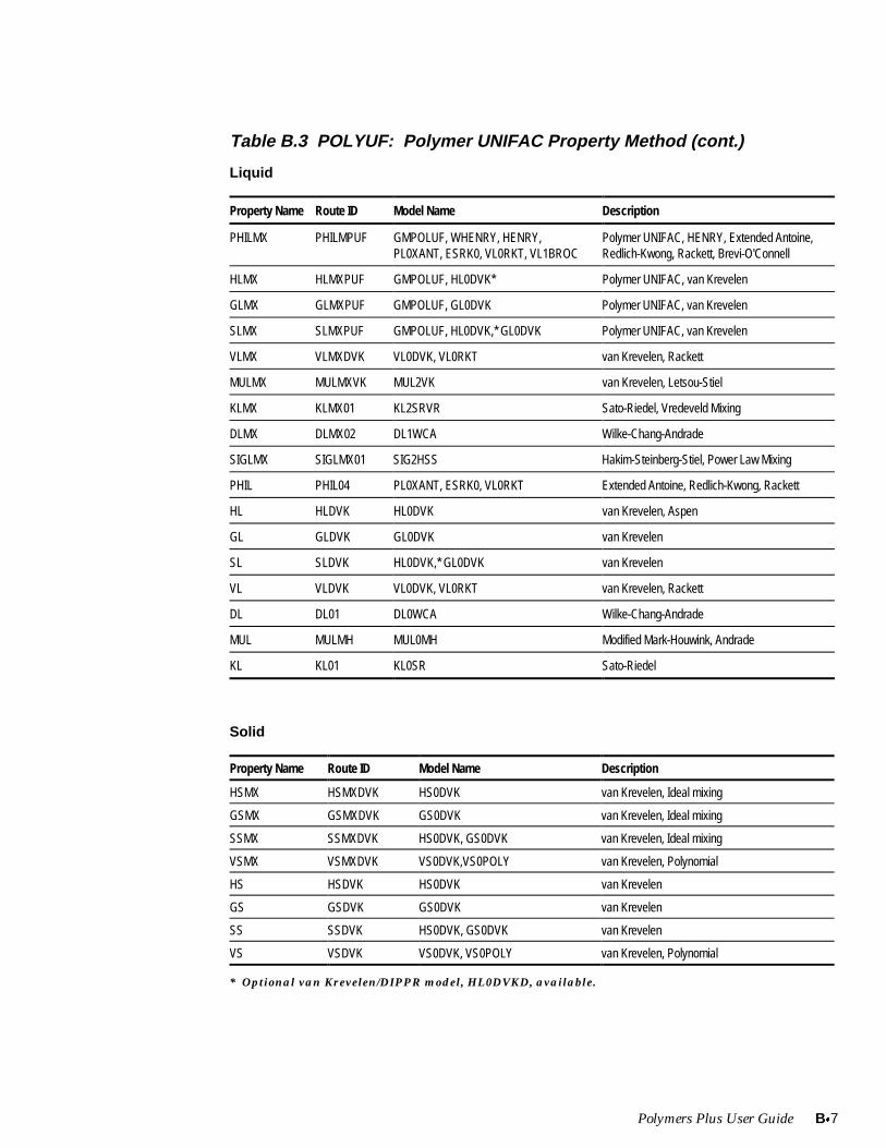
Polymers Plus User Guide Bx7
Table B.3 POLYUF: Polymer UNIFAC Property Method (cont.)
Liquid
Property Name Route ID Model Name Description
PHILMX PHILMPUF GMPOLUF, WHENRY, HENRY,PL0XANT, ESRK0, VL0RKT, VL1BROC
Polymer UNIFAC, HENRY, Extended Antoine,Redlich-Kwong, Rackett, Brevi-O'Connell
HLMX HLMXPUF GMPOLUF, HL0DVK* Polymer UNIFAC, van Krevelen
GLMX GLMXPUF GMPOLUF, GL0DVK Polymer UNIFAC, van Krevelen
SLMX SLMXPUF GMPOLUF, HL0DVK,* GL0DVK Polymer UNIFAC, van Krevelen
VLMX VLMXDVK VL0DVK, VL0RKT van Krevelen, Rackett
MULMX MULMXVK MUL2VK van Krevelen, Letsou-Stiel
KLMX KLMX01 KL2SRVR Sato-Riedel, Vredeveld Mixing
DLMX DLMX02 DL1WCA Wilke-Chang-Andrade
SIGLMX SIGLMX01 SIG2HSS Hakim-Steinberg-Stiel, Power Law Mixing
PHIL PHIL04 PL0XANT, ESRK0, VL0RKT Extended Antoine, Redlich-Kwong, Rackett
HL HLDVK HL0DVK van Krevelen, Aspen
GL GLDVK GL0DVK van Krevelen
SL SLDVK HL0DVK,* GL0DVK van Krevelen
VL VLDVK VL0DVK, VL0RKT van Krevelen, Rackett
DL DL01 DL0WCA Wilke-Chang-Andrade
MUL MULMH MUL0MH Modified Mark-Houwink, Andrade
KL KL01 KL0SR Sato-Riedel
Solid
Property Name Route ID Model Name Description
HSMX HSMXDVK HS0DVK van Krevelen, Ideal mixing
GSMX GSMXDVK GS0DVK van Krevelen, Ideal mixing
SSMX SSMXDVK HS0DVK, GS0DVK van Krevelen, Ideal mixing
VSMX VSMXDVK VS0DVK,VS0POLY van Krevelen, Polynomial
HS HSDVK HS0DVK van Krevelen
GS GSDVK GS0DVK van Krevelen
SS SSDVK HS0DVK, GS0DVK van Krevelen
VS VSDVK VS0DVK, VS0POLY van Krevelen, Polynomial
* Optional van Krevelen/DIPPR model, HL0DVKD, available.
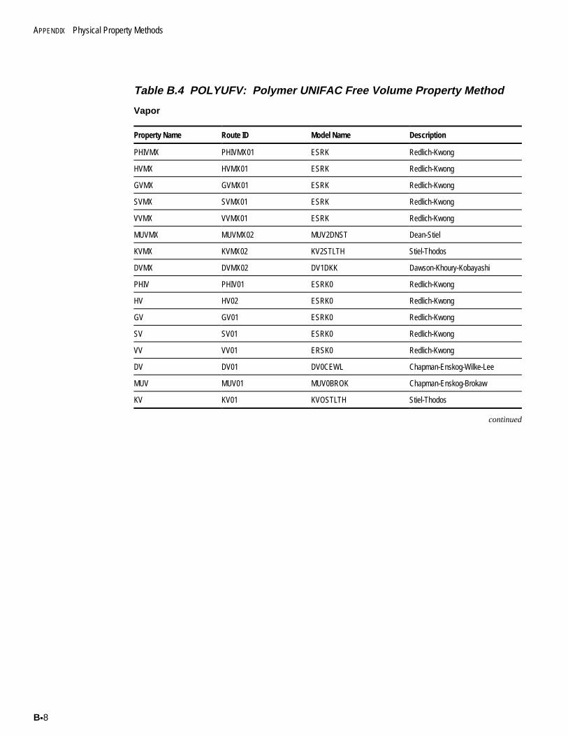
APPENDIX Physical Property Methods
Bx8
Table B.4 POLYUFV: Polymer UNIFAC Free Volume Property Method
Vapor
Property Name Route ID Model Name Description
PHIVMX PHIVMX01 ESRK Redlich-Kwong
HVMX HVMX01 ESRK Redlich-Kwong
GVMX GVMX01 ESRK Redlich-Kwong
SVMX SVMX01 ESRK Redlich-Kwong
VVMX VVMX01 ESRK Redlich-Kwong
MUVMX MUVMX02 MUV2DNST Dean-Stiel
KVMX KVMX02 KV2STLTH Stiel-Thodos
DVMX DVMX02 DV1DKK Dawson-Khoury-Kobayashi
PHIV PHIV01 ESRK0 Redlich-Kwong
HV HV02 ESRK0 Redlich-Kwong
GV GV01 ESRK0 Redlich-Kwong
SV SV01 ESRK0 Redlich-Kwong
VV VV01 ERSK0 Redlich-Kwong
DV DV01 DV0CEWL Chapman-Enskog-Wilke-Lee
MUV MUV01 MUV0BROK Chapman-Enskog-Brokaw
KV KV01 KVOSTLTH Stiel-Thodos
continued
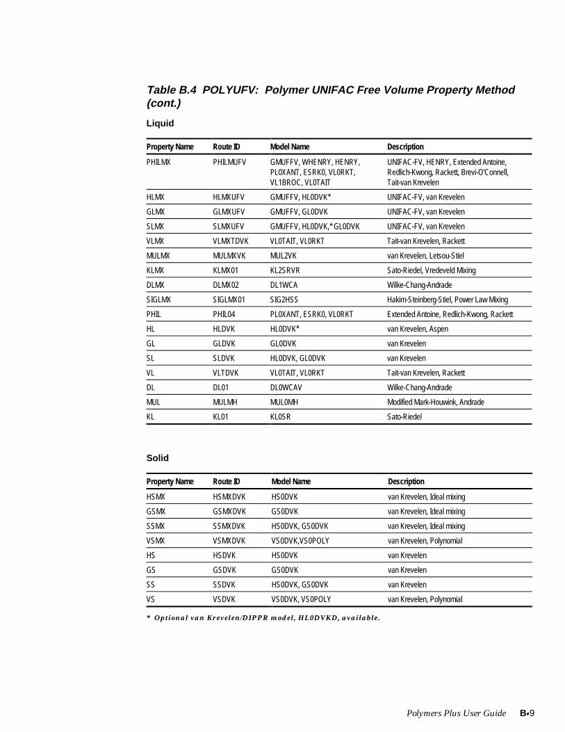
Polymers Plus User Guide Bx9
Table B.4 POLYUFV: Polymer UNIFAC Free Volume Property Method(cont.)
Liquid
Property Name Route ID Model Name Description
PHILMX PHILMUFV GMUFFV, WHENRY, HENRY,PL0XANT, ESRK0, VL0RKT,VL1BROC, VL0TAIT
UNIFAC-FV, HENRY, Extended Antoine,Redlich-Kwong, Rackett, Brevi-O'Connell,Tait-van Krevelen
HLMX HLMXUFV GMUFFV, HL0DVK* UNIFAC-FV, van Krevelen
GLMX GLMXUFV GMUFFV, GL0DVK UNIFAC-FV, van Krevelen
SLMX SLMXUFV GMUFFV, HL0DVK,* GL0DVK UNIFAC-FV, van Krevelen
VLMX VLMXTDVK VL0TAIT, VL0RKT Tait-van Krevelen, Rackett
MULMX MULMXVK MUL2VK van Krevelen, Letsou-Stiel
KLMX KLMX01 KL2SRVR Sato-Riedel, Vredeveld Mixing
DLMX DLMX02 DL1WCA Wilke-Chang-Andrade
SIGLMX SIGLMX01 SIG2HSS Hakim-Steinberg-Stiel, Power Law Mixing
PHIL PHIL04 PL0XANT, ESRK0, VL0RKT Extended Antoine, Redlich-Kwong, Rackett
HL HLDVK HL0DVK* van Krevelen, Aspen
GL GLDVK GL0DVK van Krevelen
SL SLDVK HL0DVK, GL0DVK van Krevelen
VL VLTDVK VL0TAIT, VL0RKT Tait-van Krevelen, Rackett
DL DL01 DL0WCAV Wilke-Chang-Andrade
MUL MULMH MUL0MH Modified Mark-Houwink, Andrade
KL KL01 KL0SR Sato-Riedel
Solid
Property Name Route ID Model Name Description
HSMX HSMXDVK HS0DVK van Krevelen, Ideal mixing
GSMX GSMXDVK GS0DVK van Krevelen, Ideal mixing
SSMX SSMXDVK HS0DVK, GS0DVK van Krevelen, Ideal mixing
VSMX VSMXDVK VS0DVK,VS0POLY van Krevelen, Polynomial
HS HSDVK HS0DVK van Krevelen
GS GSDVK GS0DVK van Krevelen
SS SSDVK HS0DVK, GS0DVK van Krevelen
VS VSDVK VS0DVK, VS0POLY van Krevelen, Polynomial
* Optional van Krevelen/DIPPR model, HL0DVKD, available.
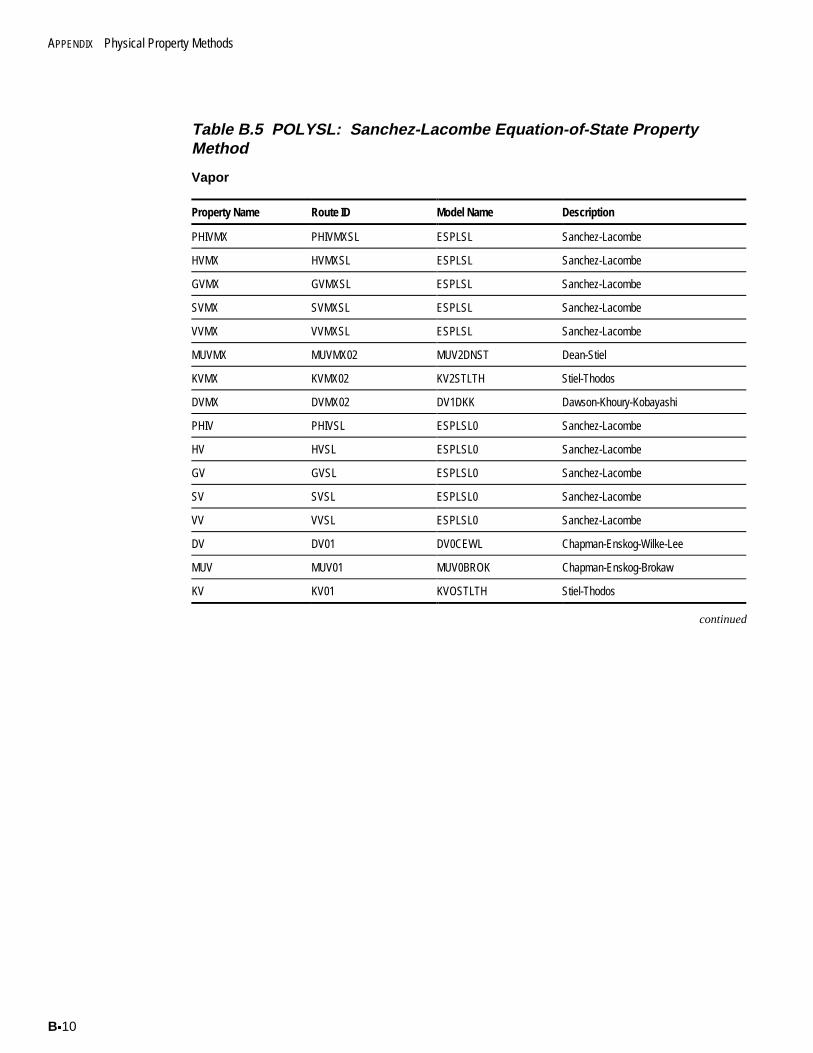
APPENDIX Physical Property Methods
Bx10
Table B.5 POLYSL: Sanchez-Lacombe Equation-of-State PropertyMethod
Vapor
Property Name Route ID Model Name Description
PHIVMX PHIVMXSL ESPLSL Sanchez-Lacombe
HVMX HVMXSL ESPLSL Sanchez-Lacombe
GVMX GVMXSL ESPLSL Sanchez-Lacombe
SVMX SVMXSL ESPLSL Sanchez-Lacombe
VVMX VVMXSL ESPLSL Sanchez-Lacombe
MUVMX MUVMX02 MUV2DNST Dean-Stiel
KVMX KVMX02 KV2STLTH Stiel-Thodos
DVMX DVMX02 DV1DKK Dawson-Khoury-Kobayashi
PHIV PHIVSL ESPLSL0 Sanchez-Lacombe
HV HVSL ESPLSL0 Sanchez-Lacombe
GV GVSL ESPLSL0 Sanchez-Lacombe
SV SVSL ESPLSL0 Sanchez-Lacombe
VV VVSL ESPLSL0 Sanchez-Lacombe
DV DV01 DV0CEWL Chapman-Enskog-Wilke-Lee
MUV MUV01 MUV0BROK Chapman-Enskog-Brokaw
KV KV01 KVOSTLTH Stiel-Thodos
continued
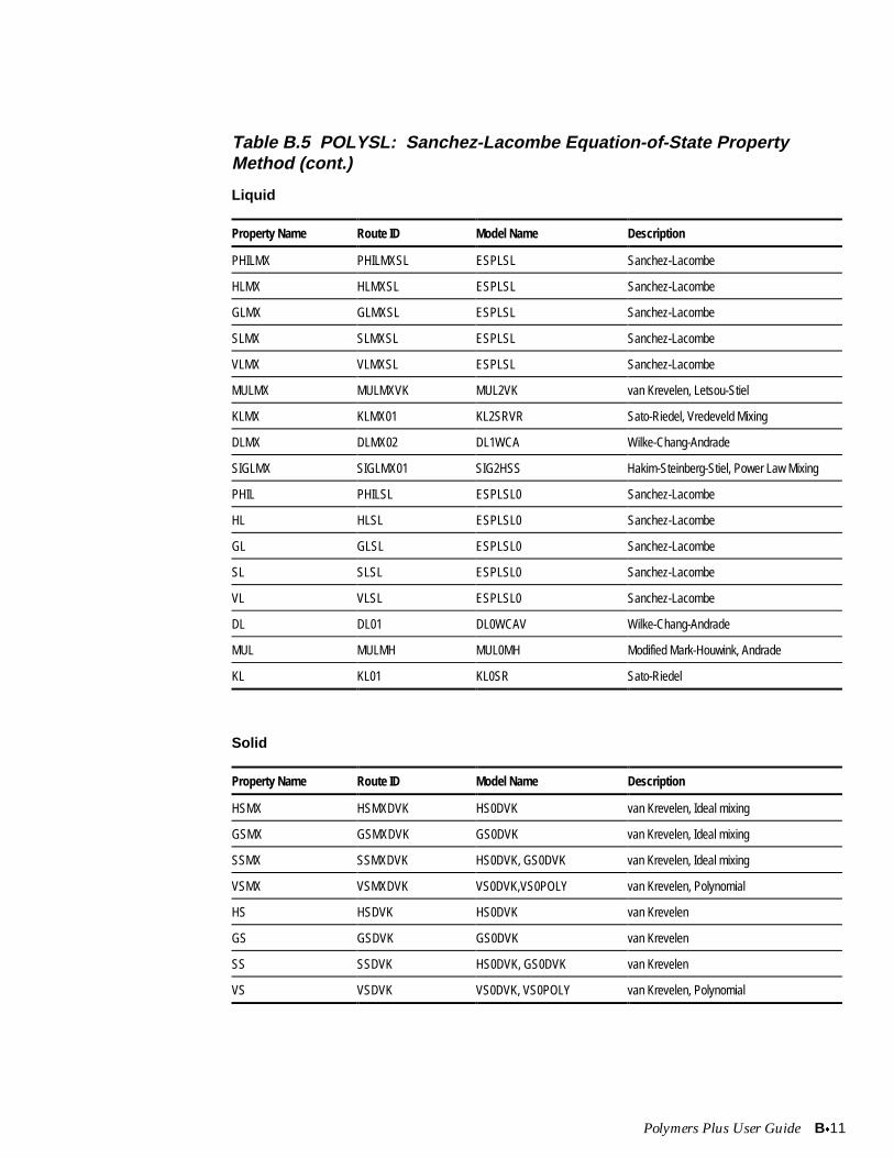
Polymers Plus User Guide Bx11
Table B.5 POLYSL: Sanchez-Lacombe Equation-of-State PropertyMethod (cont.)
Liquid
Property Name Route ID Model Name Description
PHILMX PHILMXSL ESPLSL Sanchez-Lacombe
HLMX HLMXSL ESPLSL Sanchez-Lacombe
GLMX GLMXSL ESPLSL Sanchez-Lacombe
SLMX SLMXSL ESPLSL Sanchez-Lacombe
VLMX VLMXSL ESPLSL Sanchez-Lacombe
MULMX MULMXVK MUL2VK van Krevelen, Letsou-Stiel
KLMX KLMX01 KL2SRVR Sato-Riedel, Vredeveld Mixing
DLMX DLMX02 DL1WCA Wilke-Chang-Andrade
SIGLMX SIGLMX01 SIG2HSS Hakim-Steinberg-Stiel, Power Law Mixing
PHIL PHILSL ESPLSL0 Sanchez-Lacombe
HL HLSL ESPLSL0 Sanchez-Lacombe
GL GLSL ESPLSL0 Sanchez-Lacombe
SL SLSL ESPLSL0 Sanchez-Lacombe
VL VLSL ESPLSL0 Sanchez-Lacombe
DL DL01 DL0WCAV Wilke-Chang-Andrade
MUL MULMH MUL0MH Modified Mark-Houwink, Andrade
KL KL01 KL0SR Sato-Riedel
Solid
Property Name Route ID Model Name Description
HSMX HSMXDVK HS0DVK van Krevelen, Ideal mixing
GSMX GSMXDVK GS0DVK van Krevelen, Ideal mixing
SSMX SSMXDVK HS0DVK, GS0DVK van Krevelen, Ideal mixing
VSMX VSMXDVK VS0DVK,VS0POLY van Krevelen, Polynomial
HS HSDVK HS0DVK van Krevelen
GS GSDVK GS0DVK van Krevelen
SS SSDVK HS0DVK, GS0DVK van Krevelen
VS VSDVK VS0DVK, VS0POLY van Krevelen, Polynomial
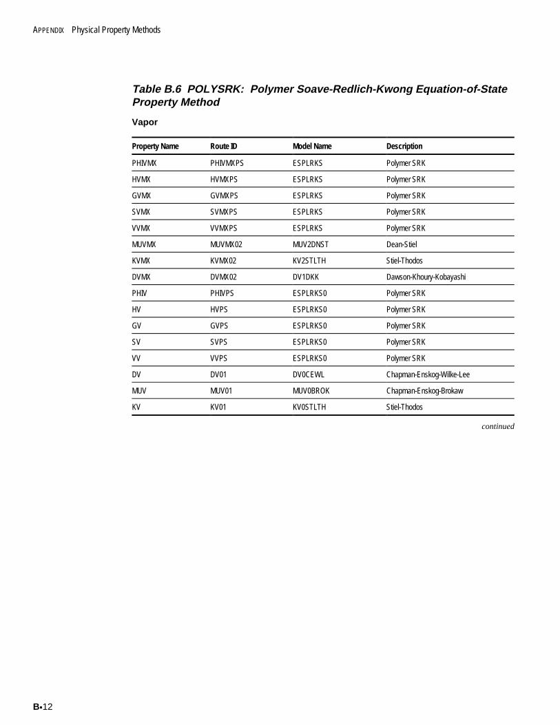
APPENDIX Physical Property Methods
Bx12
Table B.6 POLYSRK: Polymer Soave-Redlich-Kwong Equation-of-StateProperty Method
Vapor
Property Name Route ID Model Name Description
PHIVMX PHIVMXPS ESPLRKS Polymer SRK
HVMX HVMXPS ESPLRKS Polymer SRK
GVMX GVMXPS ESPLRKS Polymer SRK
SVMX SVMXPS ESPLRKS Polymer SRK
VVMX VVMXPS ESPLRKS Polymer SRK
MUVMX MUVMX02 MUV2DNST Dean-Stiel
KVMX KVMX02 KV2STLTH Stiel-Thodos
DVMX DVMX02 DV1DKK Dawson-Khoury-Kobayashi
PHIV PHIVPS ESPLRKS0 Polymer SRK
HV HVPS ESPLRKS0 Polymer SRK
GV GVPS ESPLRKS0 Polymer SRK
SV SVPS ESPLRKS0 Polymer SRK
VV VVPS ESPLRKS0 Polymer SRK
DV DV01 DV0CEWL Chapman-Enskog-Wilke-Lee
MUV MUV01 MUV0BROK Chapman-Enskog-Brokaw
KV KV01 KV0STLTH Stiel-Thodos
continued
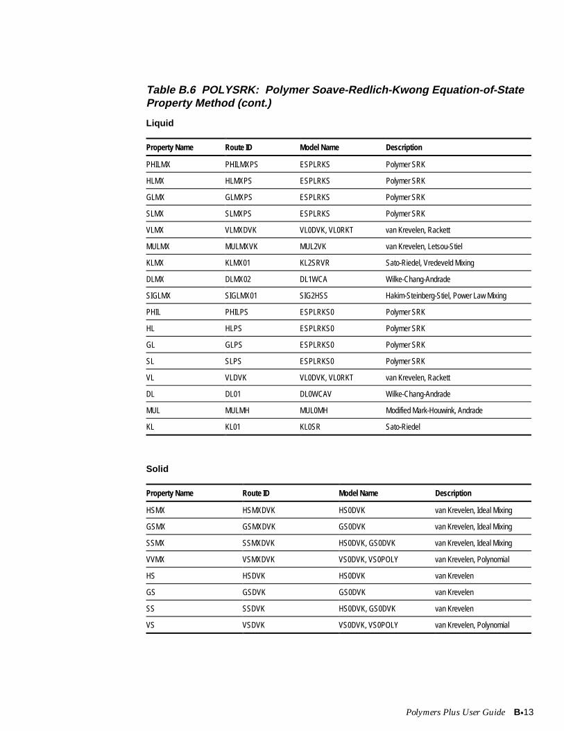
Polymers Plus User Guide Bx13
Table B.6 POLYSRK: Polymer Soave-Redlich-Kwong Equation-of-StateProperty Method (cont.)
Liquid
Property Name Route ID Model Name Description
PHILMX PHILMXPS ESPLRKS Polymer SRK
HLMX HLMXPS ESPLRKS Polymer SRK
GLMX GLMXPS ESPLRKS Polymer SRK
SLMX SLMXPS ESPLRKS Polymer SRK
VLMX VLMXDVK VL0DVK, VL0RKT van Krevelen, Rackett
MULMX MULMXVK MUL2VK van Krevelen, Letsou-Stiel
KLMX KLMX01 KL2SRVR Sato-Riedel, Vredeveld Mixing
DLMX DLMX02 DL1WCA Wilke-Chang-Andrade
SIGLMX SIGLMX01 SIG2HSS Hakim-Steinberg-Stiel, Power Law Mixing
PHIL PHILPS ESPLRKS0 Polymer SRK
HL HLPS ESPLRKS0 Polymer SRK
GL GLPS ESPLRKS0 Polymer SRK
SL SLPS ESPLRKS0 Polymer SRK
VL VLDVK VL0DVK, VL0RKT van Krevelen, Rackett
DL DL01 DL0WCAV Wilke-Chang-Andrade
MUL MULMH MUL0MH Modified Mark-Houwink, Andrade
KL KL01 KL0SR Sato-Riedel
Solid
Property Name Route ID Model Name Description
HSMX HSMXDVK HS0DVK van Krevelen, Ideal Mixing
GSMX GSMXDVK GS0DVK van Krevelen, Ideal Mixing
SSMX SSMXDVK HS0DVK, GS0DVK van Krevelen, Ideal Mixing
VVMX VSMXDVK VS0DVK, VS0POLY van Krevelen, Polynomial
HS HSDVK HS0DVK van Krevelen
GS GSDVK GS0DVK van Krevelen
SS SSDVK HS0DVK, GS0DVK van Krevelen
VS VSDVK VS0DVK, VS0POLY van Krevelen, Polynomial
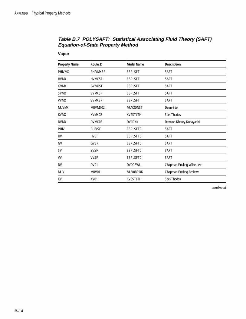
APPENDIX Physical Property Methods
Bx14
Table B.7 POLYSAFT: Statistical Associating Fluid Theory (SAFT)Equation-of-State Property Method
Vapor
Property Name Route ID Model Name Description
PHIVMX PHIVMXSF ESPLSFT SAFT
HVMX HVMXSF ESPLSFT SAFT
GVMX GVMXSF ESPLSFT SAFT
SVMX SVMXSF ESPLSFT SAFT
VVMX VVMXSF ESPLSFT SAFT
MUVMX MUVMX02 MUV2DNST Dean-Stiel
KVMX KVMX02 KV2STLTH Stiel-Thodos
DVMX DVMX02 DV1DKK Dawson-Khoury-Kobayashi
PHIV PHIVSF ESPLSFT0 SAFT
HV HVSF ESPLSFT0 SAFT
GV GVSF ESPLSFT0 SAFT
SV SVSF ESPLSFT0 SAFT
VV VVSF ESPLSFT0 SAFT
DV DV01 DV0CEWL Chapman-Enskog-Wilke-Lee
MUV MUV01 MUV0BROK Chapman-Enskog-Brokaw
KV KV01 KV0STLTH Stiel-Thodos
continued
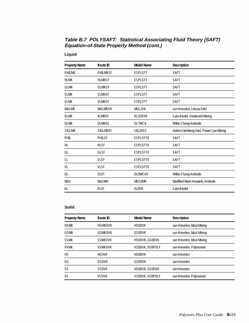
Polymers Plus User Guide Bx15
Table B.7 POLYSAFT: Statistical Associating Fluid Theory (SAFT)Equation-of-State Property Method (cont.)
Liquid
Property Name Route ID Model Name Description
PHILMX PHILMXSF ESPLSFT SAFT
HLMX HLMXSF ESPLSFT SAFT
GLMX GLMXSF ESPLSFT SAFT
SLMX SLMXSF ESPLSFT SAFT
VLMX VLMXSF ESPLSFT SAFT
MULMX MULMXVK MUL2VK van Krevelen, Letsou-Stiel
KLMX KLMX01 KL2SRVR Sato-Riedel, Vredeveld Mixing
DLMX DLMX02 DL1WCA Wilke-Chang-Andrade
SIGLMX SIGLMX01 SIG2HSS Hakim-Steinberg-Stiel, Power Law Mixing
PHIL PHILSF ESPLSFT0 SAFT
HL HLSF ESPLSFT0 SAFT
GL GLSF ESPLSFT0 SAFT
SL SLSF ESPLSFT0 SAFT
VL VLSF ESPLSFT0 SAFT
DL DL01 DL0WCAV Wilke-Chang-Andrade
MUL MULMH MUL0MH Modified Mark-Houwink, Andrade
KL KL01 KL0SR Sato-Riedel
Solid
Property Name Route ID Model Name Description
HSMX HSMXDVK HS0DVK van Krevelen, Ideal Mixing
GSMX GSMXDVK GS0DVK van Krevelen, Ideal Mixing
SSMX SSMXDVK HS0DVK, GS0DVK van Krevelen, Ideal Mixing
VVMX VSMXDVK VS0DVK, VS0POLY van Krevelen, Polynomial
HS HSDVK HS0DVK van Krevelen
GS GSDVK GS0DVK van Krevelen
SS SSDVK HS0DVK, GS0DVK van Krevelen
VS VSDVK VS0DVK, VS0POLY van Krevelen, Polynomial

APPENDIX Physical Property Methods
Bx16
Polymers Plus User Guide Cx1
C VAN KREVELEN FUNCTIONAL GROUPS
This appendix lists the van Krevelen functional group parameters. These functionalgroups used by the van Krevelen property models are listed by category:
x Hydrocarbon groups (Cx4)x Other Hydrogen-containing groups (Cx5)x Oxygen-containing groups (Cx7)x Nitrogen-containing groups (Cx8)x Sulfur-containing groups (Cx10)x Halogen-containing groups (Cx10)
C
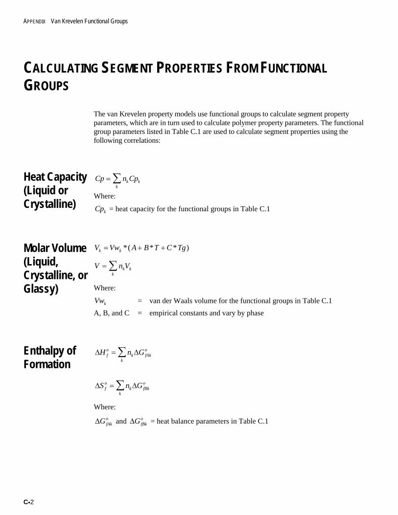
APPENDIX Van Krevelen Functional Groups
Cx2
CALCULATING SEGMENT PROPERTIES FROM FUNCTIONALGROUPS
The van Krevelen property models use functional groups to calculate segment propertyparameters, which are in turn used to calculate polymer property parameters. The functionalgroup parameters listed in Table C.1 are used to calculate segment properties using thefollowing correlations:
Heat Capacity(Liquid orCrystalline)
Cp n Cpk kk
¦
Where:
Cpk = heat capacity for the functional groups in Table C.1
Molar Volume(Liquid,Crystalline, orGlassy)
V Vw A B T C Tgk k � �*( * * )
V n Vk kk
¦
Where:
Vwk = van der Waals volume for the functional groups in Table C.1
A, B, and C = empirical constants and vary by phase
Enthalpy ofFormation
' 'H n Gfo
k fAko
k
¦
' 'S n Gfo
k fBko
k
¦
Where:
'GfAko and 'GfBk
o = heat balance parameters in Table C.1
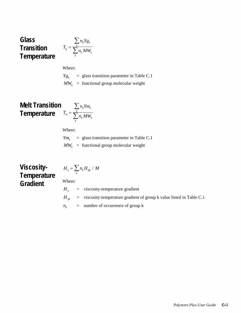
Polymers Plus User Guide Cx3
GlassTransitionTemperature
Tn Yg
n MWg
k kk
k kk
¦
¦
Where:
Ygk = glass transition parameter in Table C.1
MWk = functional group molecular weight
Melt TransitionTemperature T
n Ym
n MWm
k kk
k kk
¦
¦
Where:
Ymk = glass transition parameter in Table C.1
MWk = functional group molecular weight
Viscosity-TemperatureGradient
H n H Mk kk
K K ¦ /
Where:
HK
= viscosity-temperature gradient
H kK = viscosity-temperature gradient of group k value listed in Table C.1
nk = number of occurrence of group k
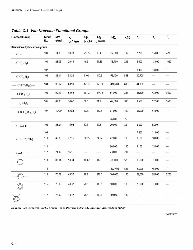
APPENDIX Van Krevelen Functional Groups
Cx4
Table C.1 Van Krevelen Functional Groups
Functional Group GroupNo.
MWg/mol
Vw
cm / mol3
Cpc
J/mol-K
Cpl
J/mol-K''GfA
o''GfB
o Yg Ym HKK
Bifunctional hydrocarbon groups
CH2100 14.03 10.23 25.35 30.4 -22,000 102 2,700 5,700 420
CH(CH3)101 28.05 20.45 46.5 57.85 -48,700 215 8,000 13,000 1060
102 8,000 13,000 ----
CH(C5H9)103 82.14 53.28 110.8 147.5 -73,400 548 30,700 ---- ----
CH(C6H11)104 96.17 63.58 121.2 173. 9 -118,400 680 41,300 ---- ----
CH(C6H5)105 90.12 52.62 101.2 144.15 84,300 287 36,100 48,000 3600
C(CH3)2106 42.08 30.67 68.0 81.2 -72,000 330 8,500 12,100 1620
C(CH3)(C6H5)107 104.14 62.84 122.7 167.5 61,000 402 51,000 54,000 ----
76,000 76
CH CH 108 26.04 16.94 37.3 42.8 70,000 83 3,800 8,000 ----
109 7,400 11,000 ----
CH C(CH3)110 40.06 27.16 60.05 74.22 42,000 183 8,100 10,000 ----
111 36,000 190 9,100 13,000 ----
C C 112 24.02 16.1 ---- ---- 230,000 -50 ---- ---- ----
113 82.14 53.34 103.2 147.5 -96,400 578 19,000 31,000 ----
114 -102,400 585 27,000 45,000 ----
115 76.09 43.32 78.8 113.1 100,000 180 29,000 38,000 3200
116 76.09 43.32 78.8 113.1 100,000 180 25,000 31,000 ----
117 76.09 43.32 78.8 113.1 100,000 180 ---- ---- ----
Source: Van Krevelen, D.W., Properties of Polymers, 3rd Ed., Elsevier, Amsterdam (1990).
continued
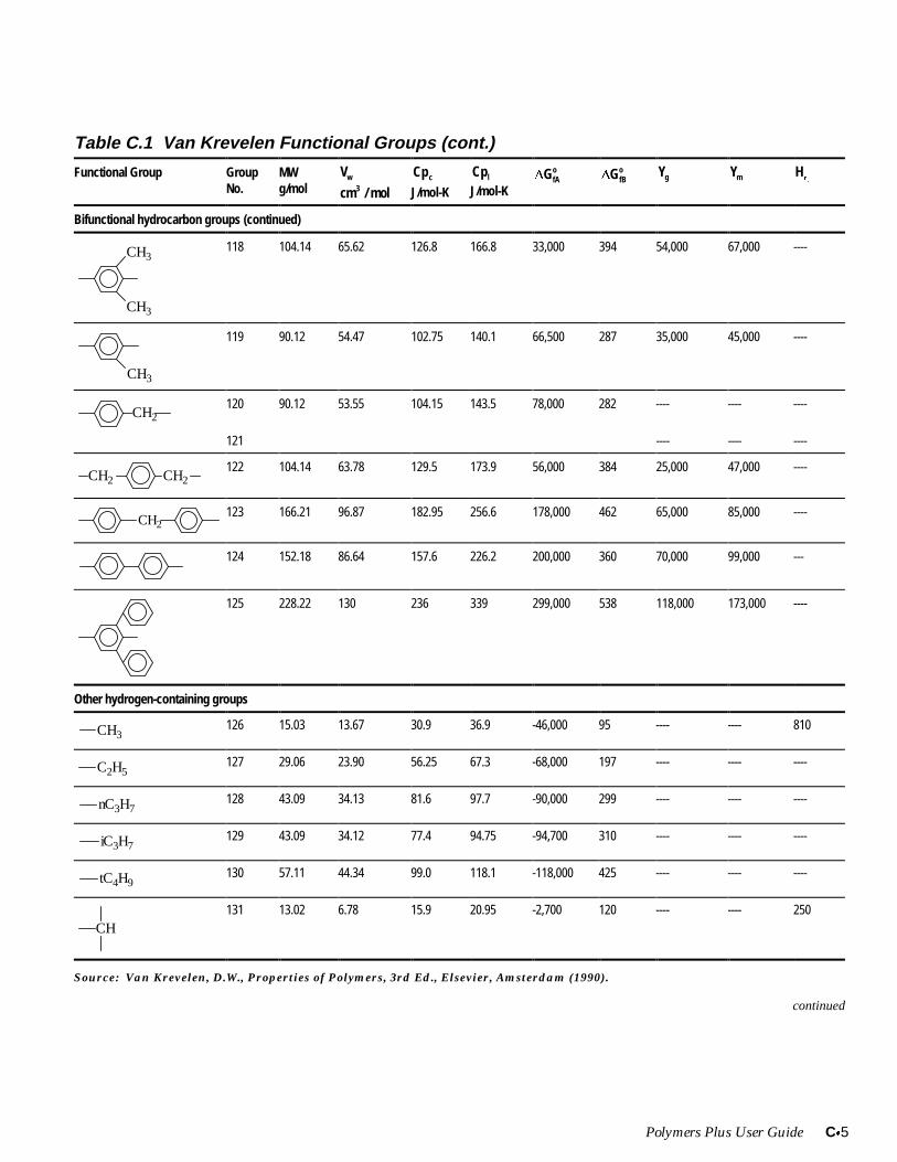
Polymers Plus User Guide Cx5
Table C.1 Van Krevelen Functional Groups (cont.)
Functional Group GroupNo.
MWg/mol
Vw
cm / mol3
Cpc
J/mol-K
Cpl
J/mol-K''GfA
o''GfB
o Yg Ym HKK
Bifunctional hydrocarbon groups (continued)
CH3
CH3
118 104.14 65.62 126.8 166.8 33,000 394 54,000 67,000 ----
CH3
119 90.12 54.47 102.75 140.1 66,500 287 35,000 45,000 ----
CH2120 90.12 53.55 104.15 143.5 78,000 282 ---- ---- ----
121 ---- ---- ----
CH2CH2122 104.14 63.78 129.5 173.9 56,000 384 25,000 47,000 ----
CH2123 166.21 96.87 182.95 256.6 178,000 462 65,000 85,000 ----
124 152.18 86.64 157.6 226.2 200,000 360 70,000 99,000 ---
125 228.22 130 236 339 299,000 538 118,000 173,000 ----
Other hydrogen-containing groups
CH3126 15.03 13.67 30.9 36.9 -46,000 95 ---- ---- 810
C2H5127 29.06 23.90 56.25 67.3 -68,000 197 ---- ---- ----
nC3H7128 43.09 34.13 81.6 97.7 -90,000 299 ---- ---- ----
iC3H7129 43.09 34.12 77.4 94.75 -94,700 310 ---- ---- ----
tC4H9130 57.11 44.34 99.0 118.1 -118,000 425 ---- ---- ----
CH131 13.02 6.78 15.9 20.95 -2,700 120 ---- ---- 250
Source: Van Krevelen, D.W., Properties of Polymers, 3rd Ed., Elsevier, Amsterdam (1990).
continued
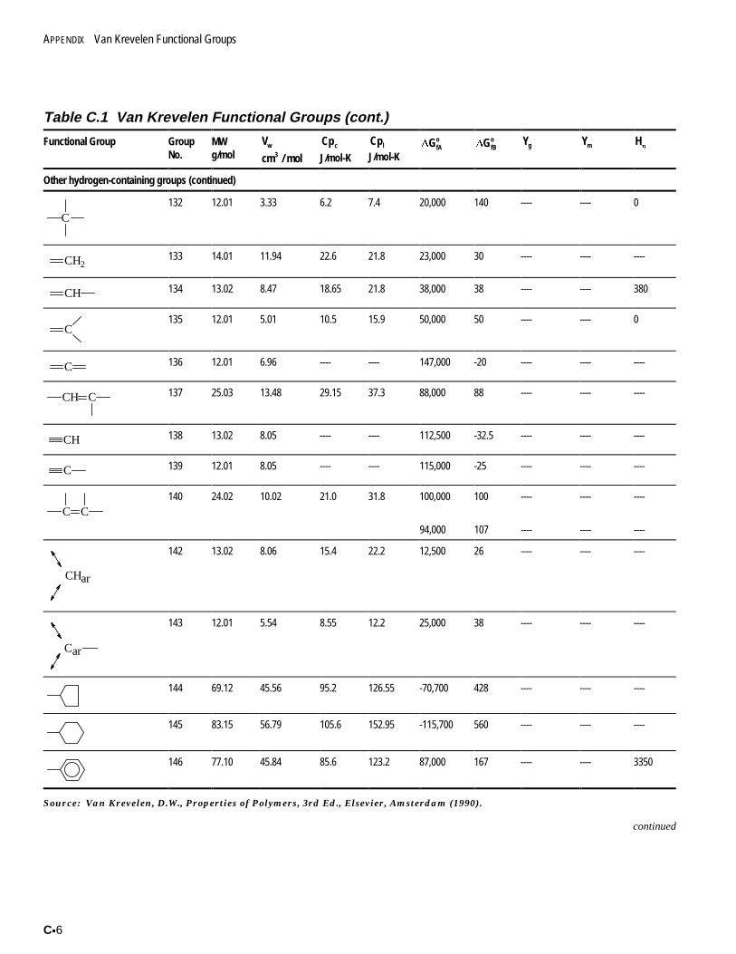
APPENDIX Van Krevelen Functional Groups
Cx6
Table C.1 Van Krevelen Functional Groups (cont.)
Functional Group GroupNo.
MWg/mol
Vw
cm / mol3
Cpc
J/mol-K
Cpl
J/mol-K''GfA
o''GfB
o Yg Ym HKK
Other hydrogen-containing groups (continued)
C132 12.01 3.33 6.2 7.4 20,000 140 ---- ---- 0
CH2133 14.01 11.94 22.6 21.8 23,000 30 ---- ---- ----
CH 134 13.02 8.47 18.65 21.8 38,000 38 ---- ---- 380
C135 12.01 5.01 10.5 15.9 50,000 50 ---- ---- 0
C 136 12.01 6.96 ---- ---- 147,000 -20 ---- ---- ----
CH C 137 25.03 13.48 29.15 37.3 88,000 88 ---- ---- ----
CH 138 13.02 8.05 ---- ---- 112,500 -32.5 ---- ---- ----
C 139 12.01 8.05 ---- ---- 115,000 -25 ---- ---- ----
C C140 24.02 10.02 21.0 31.8 100,000 100 ---- ---- ----
94,000 107 ---- ---- ----
CHar
142 13.02 8.06 15.4 22.2 12,500 26 ---- ---- ----
Car
143 12.01 5.54 8.55 12.2 25,000 38 ---- ---- ----
144 69.12 45.56 95.2 126.55 -70,700 428 ---- ---- ----
145 83.15 56.79 105.6 152.95 -115,700 560 ---- ---- ----
146 77.10 45.84 85.6 123.2 87,000 167 ---- ---- 3350
Source: Van Krevelen, D.W., Properties of Polymers, 3rd Ed., Elsevier, Amsterdam (1990).
continued
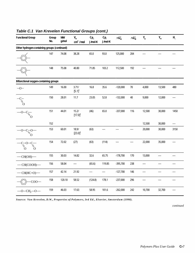
Polymers Plus User Guide Cx7
Table C.1 Van Krevelen Functional Groups (cont.)
Functional Group GroupNo.
MWg/mol
Vw
cm / mol3
Cpc
J/mol-K
Cpl
J/mol-K''GfA
o''GfB
o Yg Ym HKK
Other hydrogen-containing groups (continued)
147 74.08 38.28 65.0 93.0 125,000 204 ---- ---- ----
148 75.08 40.80 71.85 103.2 112,500 192 ---- ---- ----
Bifunctional oxygen-containing groups
O 149 16.00 3.71/[5.1]1
16.8 35.6 -120,000 70 4,000 13,500 480
C
O
150 28.01 11.7 23.05 52.8 -132,000 40 9,000 12,000 ----
O C
O
151 44.01 15.2/[17.0]1
(46) 65.0 -337,000 116 12,500 30,000 1450
152 12,500 30,000 ----
O C O
O
153 60.01 18.9/[23.0]1
(63) ---- ---- ---- 20,000 30,000 3150
C O C
O O
154 72.02 (27) (63) (114) ---- ---- 22,000 35,000 ----
CH(OH) 155 30.03 14.82 32.6 65.75 -178,700 170 13,000 ---- ----
CH(COOH) 156 58.04 ---- (65.6) 119.85 -395,700 238 ---- ---- ----
CH(HC=O) 157 42.14 21.92 ---- ---- -127,700 146 ---- ---- ----
COO158 120.10 58.52 (124.8) 178.1 -237,000 296 ---- ---- ----
O CH2 O 159 46.03 17.63 58.95 101.6 -262,000 242 10,700 32,700 ----
Source: Van Krevelen, D.W., Properties of Polymers, 3rd Ed., Elsevier, Amsterdam (1990).
continued
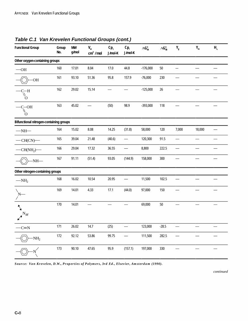
APPENDIX Van Krevelen Functional Groups
Cx8
Table C.1 Van Krevelen Functional Groups (cont.)
Functional Group GroupNo.
MWg/mol
Vw
cm / mol3
Cpc
J/mol-K
Cpl
J/mol-K''GfA
o''GfB
o Yg Ym HKK
Other oxygen-containing groups
OH 160 17.01 8.04 17.0 44.8 -176,000 50 --- ---- ----
OH161 93.10 51.36 95.8 157.9 -76,000 230 ---- ---- ----
C H
O
162 29.02 15.14 ---- ---- -125,000 26 ---- ---- ----
C OH
O
163 45.02 ---- (50) 98.9 -393,000 118 ---- ---- ----
Bifunctional nitrogen-containing groups
NH 164 15.02 8.08 14.25 (31.8) 58,000 120 7,000 18,000 ----
CH(CN) 165 39.04 21.48 (40.6) ---- 120,300 91.5 ---- ---- ----
CH(NH2)166 29.04 17.32 36.55 ---- 8,800 222.5 ---- ---- ----
NH167 91.11 (51.4) 93.05 (144.9) 158,000 300 ---- ---- ----
Other nitrogen-containing groups
NH2168 16.02 10.54 20.95 ---- 11,500 102.5 ---- ---- ----
N169 14.01 4.33 17.1 (44.0) 97,000 150 ---- ---- ----
Nar
170 14.01 ---- ---- ---- 69,000 50 ---- ---- ----
C N 171 26.02 14.7 (25) ---- 123,000 -28.5 ---- ---- ----
NH2172 92.12 53.86 99.75 ---- 111,500 282.5 ---- ---- ----
N173 90.10 47.65 95.9 (157.1) 197,000 330 ---- ---- ----
Source: Van Krevelen, D.W., Properties of Polymers, 3rd Ed., Elsevier, Amsterdam (1990).
continued
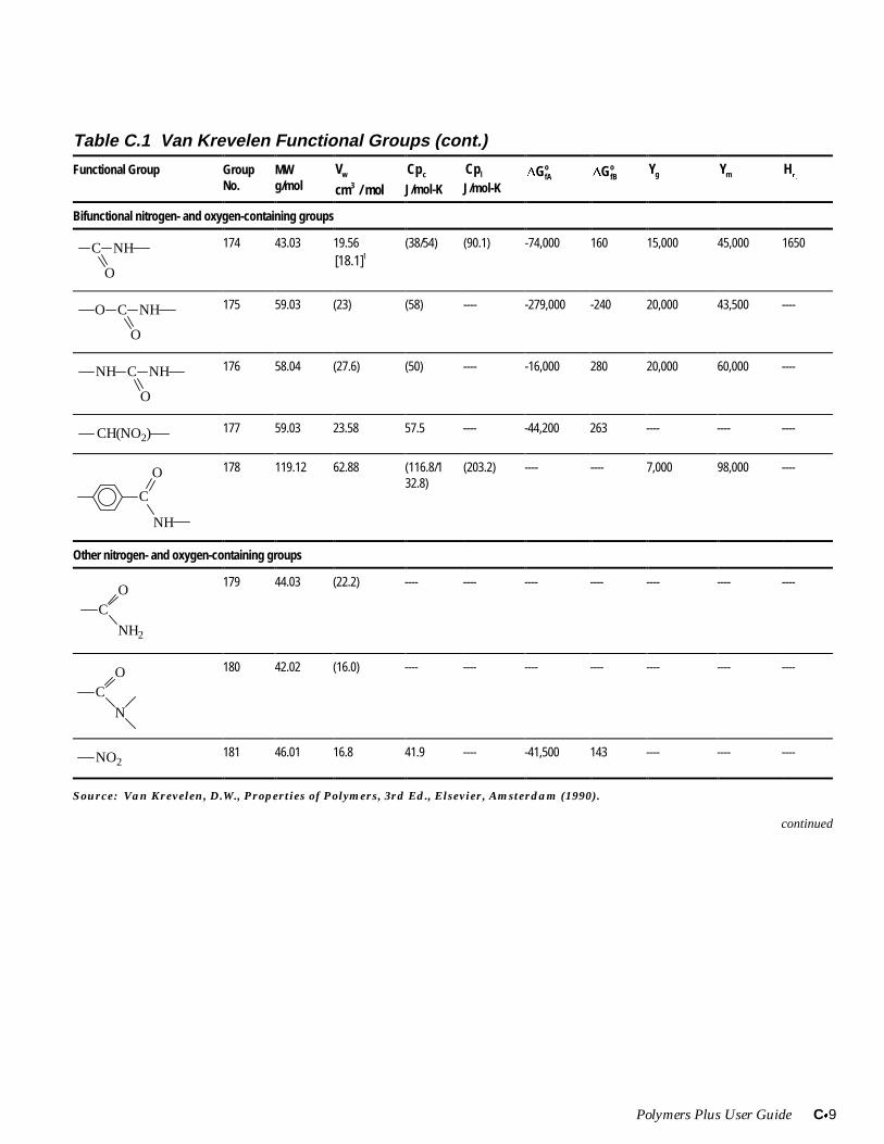
Polymers Plus User Guide Cx9
Table C.1 Van Krevelen Functional Groups (cont.)
Functional Group GroupNo.
MWg/mol
Vw
cm / mol3
Cpc
J/mol-K
Cpl
J/mol-K''GfA
o''GfB
o Yg Ym HKK
Bifunctional nitrogen- and oxygen-containing groups
C NH
O
174 43.03 19.56[18.1]1
(38/54) (90.1) -74,000 160 15,000 45,000 1650
O C NH
O
175 59.03 (23) (58) ---- -279,000 -240 20,000 43,500 ----
NH C NH
O
176 58.04 (27.6) (50) ---- -16,000 280 20,000 60,000 ----
CH(NO2)177 59.03 23.58 57.5 ---- -44,200 263 ---- ---- ----
C
NH
O 178 119.12 62.88 (116.8/132.8)
(203.2) ---- ---- 7,000 98,000 ----
Other nitrogen- and oxygen-containing groups
CO
NH2
179 44.03 (22.2) ---- ---- ---- ---- ---- ---- ----
CO
N
180 42.02 (16.0) ---- ---- ---- ---- ---- ---- ----
NO2181 46.01 16.8 41.9 ---- -41,500 143 ---- ---- ----
Source: Van Krevelen, D.W., Properties of Polymers, 3rd Ed., Elsevier, Amsterdam (1990).
continued
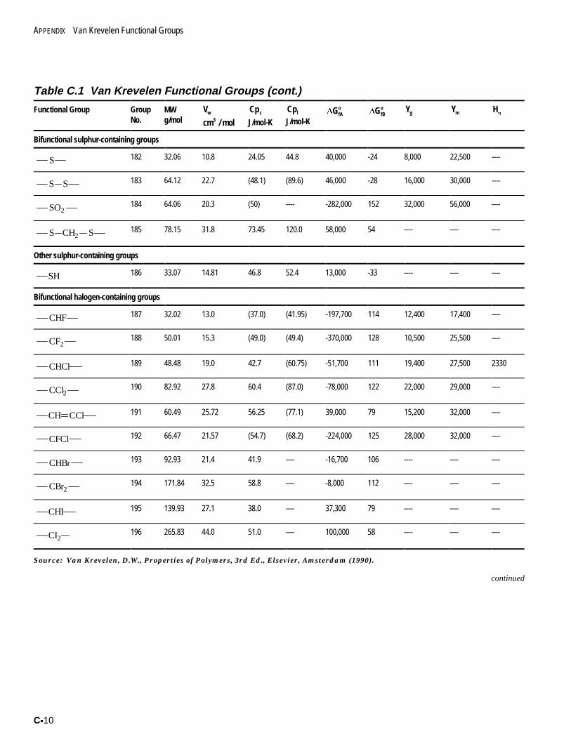
APPENDIX Van Krevelen Functional Groups
Cx10
Table C.1 Van Krevelen Functional Groups (cont.)
Functional Group GroupNo.
MWg/mol
Vw
cm / mol3
Cpc
J/mol-K
Cpl
J/mol-K''GfA
o''GfB
o Yg Ym HKK
Bifunctional sulphur-containing groups
S 182 32.06 10.8 24.05 44.8 40,000 -24 8,000 22,500 ----
S S 183 64.12 22.7 (48.1) (89.6) 46,000 -28 16,000 30,000 ----
SO2184 64.06 20.3 (50) ---- -282,000 152 32,000 56,000 ----
S CH2 S 185 78.15 31.8 73.45 120.0 58,000 54 ---- ---- ----
Other sulphur-containing groups
SH 186 33.07 14.81 46.8 52.4 13,000 -33 ---- ---- ----
Bifunctional halogen-containing groups
CHF 187 32.02 13.0 (37.0) (41.95) -197,700 114 12,400 17,400 ----
CF2188 50.01 15.3 (49.0) (49.4) -370,000 128 10,500 25,500 ----
CHCl 189 48.48 19.0 42.7 (60.75) -51,700 111 19,400 27,500 2330
CCl2190 82.92 27.8 60.4 (87.0) -78,000 122 22,000 29,000 ----
CH CCl 191 60.49 25.72 56.25 (77.1) 39,000 79 15,200 32,000 ----
CFCl 192 66.47 21.57 (54.7) (68.2) -224,000 125 28,000 32,000 ----
CHBr 193 92.93 21.4 41.9 ---- -16,700 106 ---- ---- ----
CBr2194 171.84 32.5 58.8 ---- -8,000 112 ---- ---- ----
CHI 195 139.93 27.1 38.0 ---- 37,300 79 ---- ---- ----
CI2196 265.83 44.0 51.0 ---- 100,000 58 ---- ---- ----
Source: Van Krevelen, D.W., Properties of Polymers, 3rd Ed., Elsevier, Amsterdam (1990).
continued
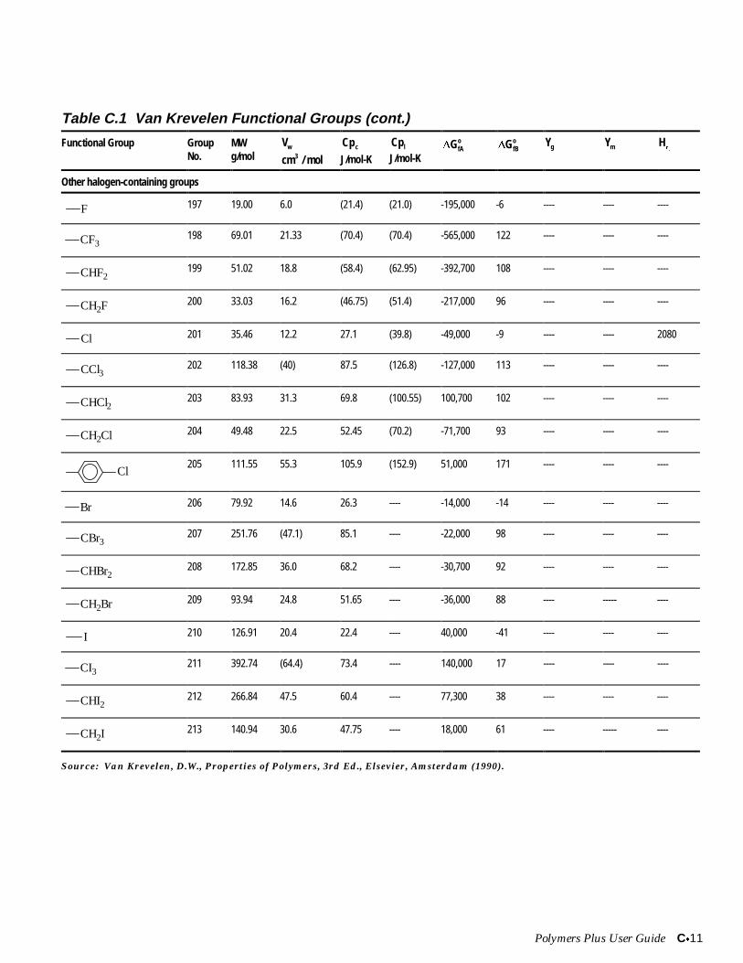
Polymers Plus User Guide Cx11
Table C.1 Van Krevelen Functional Groups (cont.)
Functional Group GroupNo.
MWg/mol
Vw
cm / mol3
Cpc
J/mol-K
Cpl
J/mol-K''GfA
o''GfB
o Yg Ym HKK
Other halogen-containing groups
F 197 19.00 6.0 (21.4) (21.0) -195,000 -6 ---- ---- ----
CF3198 69.01 21.33 (70.4) (70.4) -565,000 122 ---- ---- ----
CHF2199 51.02 18.8 (58.4) (62.95) -392,700 108 ---- ---- ----
CH2F200 33.03 16.2 (46.75) (51.4) -217,000 96 ---- ---- ----
Cl 201 35.46 12.2 27.1 (39.8) -49,000 -9 ---- ---- 2080
CCl3202 118.38 (40) 87.5 (126.8) -127,000 113 ---- ---- ----
CHCl2203 83.93 31.3 69.8 (100.55) 100,700 102 ---- ---- ----
CH2Cl 204 49.48 22.5 52.45 (70.2) -71,700 93 ---- ---- ----
Cl205 111.55 55.3 105.9 (152.9) 51,000 171 ---- ---- ----
Br 206 79.92 14.6 26.3 ---- -14,000 -14 ---- ---- ----
CBr3207 251.76 (47.1) 85.1 ---- -22,000 98 ---- ---- ----
CHBr2208 172.85 36.0 68.2 ---- -30,700 92 ---- ---- ----
CH2Br 209 93.94 24.8 51.65 ---- -36,000 88 ---- ----- ----
I 210 126.91 20.4 22.4 ---- 40,000 -41 ---- ---- ----
CI3211 392.74 (64.4) 73.4 ---- 140,000 17 ---- ---- ----
CHI2212 266.84 47.5 60.4 ---- 77,300 38 ---- ---- ----
CH2I213 140.94 30.6 47.75 ---- 18,000 61 ---- ----- ----
Source: Van Krevelen, D.W., Properties of Polymers, 3rd Ed., Elsevier, Amsterdam (1990).

APPENDIX Van Krevelen Functional Groups
Cx12
Polymers Plus User Guide Dx1
D TAIT MODEL COEFFICIENTS
This appendix lists parameters available for the Tait molar volume calculations forselected polymers.
These parameters are available in POLYMER for the polymers listed in Table D.1.
D
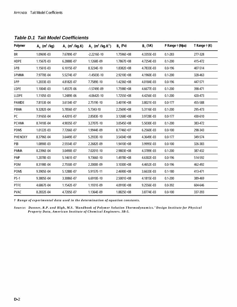
APPENDIX Tait Model Coefficients
Dx2
Table D.1 Tait Model Coefficients
Polymer A0 (m / kg)3 A1
(m / kg.K)3 A2 (m / kg.K )3 2 B0
(Pa) B1 (1/K) P Range † (Mpa) T Range † (K)
BR 1.0969E-03 7.6789E-07 -2.2216E-10 1.7596E+08 4.3355E-03 0.1-283 277-328
HDPE 1.1567E-03 6.2888E-07 1.1268E-09 1.7867E+08 4.7254E-03 0.1-200 415-472
I-PB 1.1561E-03 6.1015E-07 8.3234E-10 1.8382E+08 4.7833E-03 0.0-196 407-514
I-PMMA 7.9770E-04 5.5274E-07 -1.4503E-10 2.9210E+08 4.1960E-03 0.1-200 328-463
I-PP 1.2033E-03 4.8182E-07 7.7589E-10 1.4236E+08 4.0184E-03 0.0-196 447-571
LDPE 1.1004E-03 1.4557E-06 -1.5749E-09 1.7598E+08 4.6677E-03 0.1-200 398-471
LLDPE 1.1105E-03 1.2489E-06 -4.0642E-10 1.7255E+08 4.4256E-03 0.1-200 420-473
PAMIDE 7.8153E-04 3.6134E-07 2.7519E-10 3.4019E+08 3.8021E-03 0.0-177 455-588
PBMA 9.3282E-04 5.7856E-07 5.7343-10 2.2569E+08 5.3116E-03 0.1-200 295-473
PC 7.9165E-04 4.4201E-07 2.8583E-10 3.1268E+08 3.9728E-03 0.0-177 430-610
PCHMA 8.7410E-04 4.9035E-07 3.2707E-10 3.0545E+08 5.5030E-03 0.1-200 383-472
PDMS 1.0122E-03 7.7266E-07 1.9944E-09 8.7746E+07 6.2560E-03 0.0-100 298-343
PHENOXY 8.3796E-04 3.6449E-07 5.2933E-10 3.5434E+08 4.3649E-03 0.0-177 349-574
PIB 1.0890E-03 2.5554E-07 2.2682E-09 1.9410E+08 3.9995E-03 0.0-100 326-383
PMMA 8.2396E-04 3.0490E-07 7.0201E-10 2.9803E+08 4.3789E-03 0.1-200 387-432
PMP 1.2078E-03 5.1461E-07 9.7366E-10 1.4978E+08 4.6302E-03 0.0-196 514-592
POM 8.3198E-04 2.7550E-07 2.2000E-09 3.1030E+08 4.4652E-03 0.0-196 462-492
POMS 9.3905E-04 5.1288E-07 5.9157E-11 2.4690E+08 3.6633E-03 0.1-180 413-471
PS-1 9.3805E-04 3.3086E-07 6.6910E-10 2.5001E+08 4.1815E-03 0.1-200 389-469
PTFE 4.6867E-04 1.1542E-07 1.1931E-09 4.0910E+08 9.2556E-03 0.0-392 604-646
PVAC 8.2832E-04 4.7205E-07 1.1364E-09 1.8825E+08 3.8774E-03 0.0-100 337-393
† Range of experimental data used in the determination of equation constants.
Source: Danner, R.P. and High, M.S. "Handbook of Polymer Solution Thermodynamics." Design Institute for PhysicalProperty Data, American Institute of Chemical Engineers. 3B-5.
Polymers Plus User Guide Ex1
E MASS BASED PROPERTY PARAMETERS
The Aspen Plus convention is to use mole based parameters for property modelcalculations. However, polymer property parameters are often more convenientlyobtained on a mass basis. To satisfy the needs of users who may prefer the use of massbased parameters, in Polymers Plus there is a corresponding mass based parameter forselected mole based parameters.
Table E.1 shows a list of model parameters and their mass-based counterparts. Note thatthe mass based parameters should only be used for polymers and oligomers, and not forsegments.
E
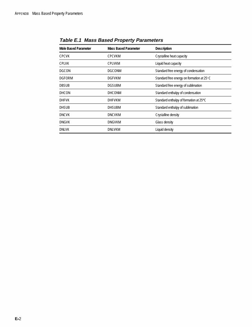
APPENDIX Mass Based Property Parameters
Ex2
Table E.1 Mass Based Property Parameters
Mole Based Parameter Mass Based Parameter Description
CPCVK CPCVKM Crystalline heat capacity
CPLVK CPLVKM Liquid heat capacity
DGCON DGCONM Standard free energy of condensation
DGFORM DGFVKM Standard free energy on formation at 25qC
DBSUB DGSUBM Standard free energy of sublimation
DHCON DHCONM Standard enthalpy of condensation
DHFVK DHFVKM Standard enthalpy of formation at 25qC
DHSUB DHSUBM Standard enthalpy of sublimation
DNCVK DNCVKM Crystalline density
DNGVK DNGVKM Glass density
DNLVK DNLVKM Liquid density
Polymers Plus User Guide Fx1
F EQUATION-OF-STATE PARAMETERS
This appendix lists unary parameters available for use with the Sanchez-Lacombeequation of state model (POLYSL property method) and the SAFT (POLYSAFT)equation of state model. Parameters are available for selected:
x Polymers (SL) (Fx2)x Monomers (SL) (Fx3)x Solvents (SL) (Fx3)x Solvents and Polymers (SAFT) (Fx6)
The parameters are not automatically retrieved from databanks. These parameters are notunique in any way. Users may generate them through experimental data regression for thecomponents of interest.
Table F.1 lists the Sanchez-Lacombe unary parameters for polymers while Table F.2 liststhe Sanchez-Lacombe unary parameters for monomers and solvents. Table F.3 lists theSAFT unary parameters for solvents, monomers and polymers.
F
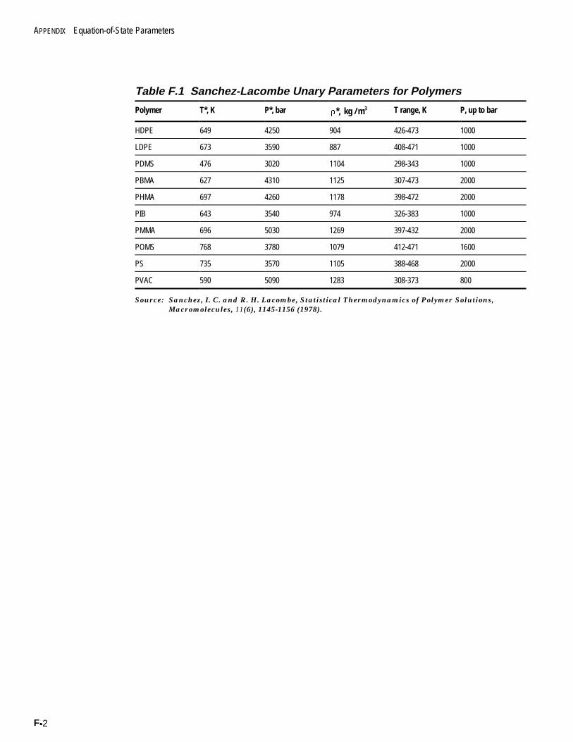
APPENDIX Equation-of-State Parameters
Fx2
Table F.1 Sanchez-Lacombe Unary Parameters for Polymers
Polymer T*, K P*, bar UU*, kg / m3 T range, K P, up to bar
HDPE 649 4250 904 426-473 1000
LDPE 673 3590 887 408-471 1000
PDMS 476 3020 1104 298-343 1000
PBMA 627 4310 1125 307-473 2000
PHMA 697 4260 1178 398-472 2000
PIB 643 3540 974 326-383 1000
PMMA 696 5030 1269 397-432 2000
POMS 768 3780 1079 412-471 1600
PS 735 3570 1105 388-468 2000
PVAC 590 5090 1283 308-373 800
Source: Sanchez, I. C. and R. H. Lacombe, Statistical Thermodynamics of Polymer Solutions,Macromolecules, 11(6), 1145-1156 (1978).
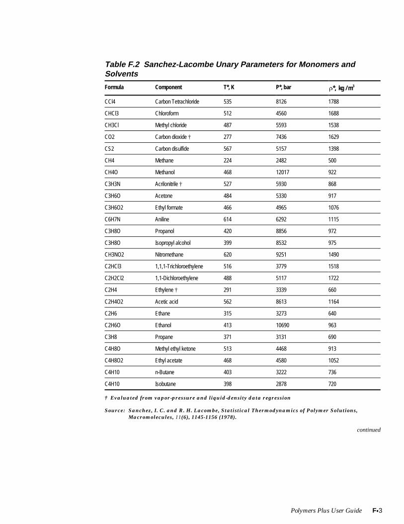
Polymers Plus User Guide Fx3
Table F.2 Sanchez-Lacombe Unary Parameters for Monomers andSolvents
Formula Component T*, K P*, bar UU*, kg / m3
CCl4 Carbon Tetrachloride 535 8126 1788
CHCl3 Chloroform 512 4560 1688
CH3Cl Methyl chloride 487 5593 1538
CO2 Carbon dioxide † 277 7436 1629
CS2 Carbon disulfide 567 5157 1398
CH4 Methane 224 2482 500
CH4O Methanol 468 12017 922
C3H3N Acrilonitrile † 527 5930 868
C3H6O Acetone 484 5330 917
C3H6O2 Ethyl formate 466 4965 1076
C6H7N Aniline 614 6292 1115
C3H8O Propanol 420 8856 972
C3H8O Isopropyl alcohol 399 8532 975
CH3NO2 Nitromethane 620 9251 1490
C2HCl3 1,1,1-Trichloroethylene 516 3779 1518
C2H2Cl2 1,1-Dichloroethylene 488 5117 1722
C2H4 Ethylene † 291 3339 660
C2H4O2 Acetic acid 562 8613 1164
C2H6 Ethane 315 3273 640
C2H6O Ethanol 413 10690 963
C3H8 Propane 371 3131 690
C4H8O Methyl ethyl ketone 513 4468 913
C4H8O2 Ethyl acetate 468 4580 1052
C4H10 n-Butane 403 3222 736
C4H10 Isobutane 398 2878 720
† Evaluated from vapor-pressure and liquid-density data regression
Source: Sanchez, I. C. and R. H. Lacombe, Statistical Thermodynamics of Polymer Solutions,Macromolecules, 11(6), 1145-1156 (1978).
continued
APPENDIX Equation-of-State Parameters
Fx4
Table F.2 Sanchez-Lacombe Unary Parameters for Monomers andSolvents (cont.)
Formula Component T*, K P*, bar UU*, kg / m3
C4H10O Tert-butyl alcohol 448 6931 952
C4H10O Diethyl ether 431 3627 870
C5H5N Pyridine 566 5492 1079
C5H10 Cyclopentane 491 3800 867
C5H12 n-Pentane 441 3101 755
C5H12 Isopentane 424 3080 765
C5H12 Neopentane 415 2655 744
C6H5Cl Chlorobenzene 585 4367 1206
C6H6 Benzene 523 4438 994
C6H6O Phenol 530 7934 1192
C6H14 n-Hexane 476 2979 775
C6H12 Cyclohexane 497 3830 902
C6H12O2 n-Butyl acetate 498 3942 1003
C7H8 Toluene 543 4023 966
C7H16 n-Heptane 487 3090 800
C8H8 Styrene † 563 3684 870
C8H10 p-Xylene 561 3810 949
C8H10 m-Xylene 560 3850 952
C8H10 o-Xylene 571 3942 965
C8H18 n-Octane 502 3080 815
C9H20 n-Nonane 517 3070 828
C10H18 trans-Decalin 621 3151 935
C10H18 cis-Decalin 631 3334 960
† Evaluated from vapor-pressure and liquid-density data regression
Source: Sanchez, I. C. and R. H. Lacombe, Statistical Thermodynamics of Polymer Solutions,Macromolecules, 11(6), 1145-1156 (1978).
continued
Polymers Plus User Guide Fx5
Table F.2 Sanchez-Lacombe Unary Parameters for Monomers andSolvents (cont.)
Formula Component T*, K P*, bar UU*, kg / m3
C10H22 n-Decane 530 3040 837
C11H24 n-Undecane 542 3030 846
C12H26 n-Dodecane 552 3009 854
C13H28 n-Tridecane 560 2989 858
C14H10 Phenanthrene 801 3769 1013
C14H30 n-Tetradecane 570 2959 864
C17H36 n-Heptadecane 596 2867 880
C20H42 n-Eicosane † 617 3067 961
H2O Water 623 26871 1105
H2S Hydrogen Sulfate 382 6129 1095
† Evaluated from vapor-pressure and liquid-density data regression
Source: Sanchez, I. C. and R. H. Lacombe, Statistical Thermodynamics of Polymer Solutions,Macromolecules, 11(6), 1145-1156 (1978).
APPENDIX Equation-of-State Parameters
Fx6
Table F.3 SAFT Unary Parameters for Various Non-Associating Fluids
Formula Component T range, K v , cm / moloo 3 m u / k, Ko
N2 Nitrogen --- 19.457 1.0 123.53
AR Argon --- 16.29 1.0 150.86
CO Carbon Monoxide 72-121 15.776 1.221 111.97
CO2 Carbon Dioxide 218-288 13.578 1.417 216.08
CL2 Chlorine 180-400 22.755 1.147 367.44
CS2 Carbon Disulfide 278-533 23.622 1.463 396.05
SO2 Sulfur Dioxide 283-413 22.611 1.133 335.84
CH4 Methane 92-180 21.576 1.0 190.29
C2H6 Ethane 160-300 14.460 1.941 191.44
C3H8 Propane 190-360 13.457 2.696 193.03
C4H10 n-Butane 220-420 12.599 3.458 195.11
C5H12 n-Pentane 233-450 12.533 4.091 200.02
C6H14 n-Hexane 243-493 12.475 4.724 202.72
C7H16 n-Heptane 273-523 12.282 5.391 204.61
C8H18 n-Octane 303-543 12.234 6.045 206.03
C9H20 n-Nonane 303-503 12.240 6.883 203.56
C10H22 n-Decane 313-573 11.723 7.527 205.46
C12H26 n-Dodecane 313-523 11.864 8.921 205.93
C14H30 n-Tetradecane 313-533 12.389 9.978 209.40
C16H34 n-Hexadecane 333-593 12.300 11.209 210.65
C20H42 n-Eicosane 393-573 12.0 13.940 211.25
C28H58 n-Octacosane 449-704 12.0 19.287 209.96
C36H74 n-Hexatriacontane 497-768 12.0 24.443 208.74
C44H90 n-Tetratetracontane 534-725 12.0 29.252 207.73
C5H10 Cyclopentane 252-483 12.469 3.670 226.70
C6H12 Methyl-cyclopentane 263-503 13.201 4.142 223.25
C7H14 Ethyl-cyclopentane 273-513 13.766 4.578 229.04
C8H16 Propyl-cyclopentane 293-423 14.251 5.037 232.18
continued
Source: Huang, S. H. and M. Radosz, Equation of State for Small, Large, Polydisperse, andAssociating Molecules, Ind., Eng. Chem. Res., 29, 2284-2294 (1990).
Polymers Plus User Guide Fx7
Table F.3 SAFT Unary Parameters for Various Non-Associating Fluids(cont.)
Formula Component T range, K v , cm / moloo 3 m u / k, Ko
C9H18 Butyl-cyclopentane 314-578 14.148 5.657 230.61
C10H20 Pentyl-cyclopentane 333-483 13.460 6.503 225.56
C6H12 Cyclohexane 283-513 13.502 3.970 236.41
C7H14 Methylcyclohexane 273-533 15.651 3.954 248.44
C8H16 Ethylcyclohexane 273-453 15.503 4.656 243.16
C9H18 Propylcyclohexane 313-453 15.037 5.326 238.51
C10H20 Butylcyclohexane 333-484 14.450 6.060 234.30
C11H22 Pentylcyclohexane 353-503 14.034 6.804 230.91
C6H6 Benzene 300-540 11.421 3.749 250.19
C7H8 Methyl-benzene 293-533 11.789 4.373 245.27
C8H10 Ethyl-benzene 293-573 12.681 4.719 248.79
C9H12 n-Propyl-benzene 323-573 12.421 5.521 238.66
C10H14 n-Butyl-benzene 293-523 12.894 6.058 238.19
C8H10 m-Xylene 309-573 12.184 4.886 245.88
C12H10 Biphenyl 433-653 12.068 6.136 280.54
C10H8 Naphthalene 373-693 13.704 4.671 304.80
C11H10 1-Methyl-naphthalene 383-511 13.684 5.418 293.45
C12H12 1-Ethyl-naphthalene 393-563 12.835 6.292 276.18
C13H14 1-n-Propyl-naphthalene 403-546 13.304 6.882 266.82
C14H16 1-n-Butyl-naphthalene 413-566 13.140 7.766 252.11
C14H10 Phenanthrene 373-633 16.518 5.327 352.00
C14H10 Anthracene 493-673 16.297 5.344 352.65
C16H10 Pyrene 553-673 18.212 5.615 369.38
C2H6O Dimethyl-ether 179-265 11.536 2.799 207.83
C3H8O Methyl-ethyl-ether 266-299 10.065 3.540 203.54
C4H10O methyl-n-propyl-ether 267-335 10.224 4.069 208.13
continued
Source: Huang, S. H. and M. Radosz, Equation of State for Small, Large, Polydisperse, andAssociating Molecules, Ind., Eng. Chem. Res., 29, 2284-2294 (1990).
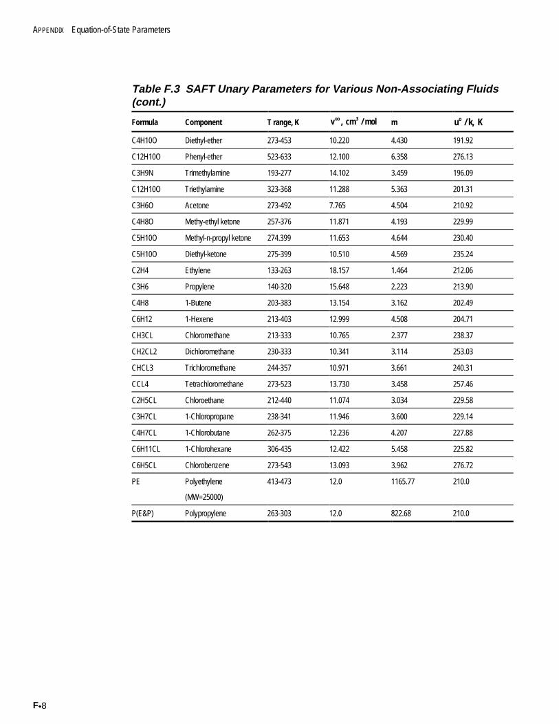
APPENDIX Equation-of-State Parameters
Fx8
Table F.3 SAFT Unary Parameters for Various Non-Associating Fluids(cont.)
Formula Component T range, K v , cm / moloo 3 m u / k, Ko
C4H10O Diethyl-ether 273-453 10.220 4.430 191.92
C12H10O Phenyl-ether 523-633 12.100 6.358 276.13
C3H9N Trimethylamine 193-277 14.102 3.459 196.09
C12H10O Triethylamine 323-368 11.288 5.363 201.31
C3H6O Acetone 273-492 7.765 4.504 210.92
C4H8O Methy-ethyl ketone 257-376 11.871 4.193 229.99
C5H10O Methyl-n-propyl ketone 274.399 11.653 4.644 230.40
C5H10O Diethyl-ketone 275-399 10.510 4.569 235.24
C2H4 Ethylene 133-263 18.157 1.464 212.06
C3H6 Propylene 140-320 15.648 2.223 213.90
C4H8 1-Butene 203-383 13.154 3.162 202.49
C6H12 1-Hexene 213-403 12.999 4.508 204.71
CH3CL Chloromethane 213-333 10.765 2.377 238.37
CH2CL2 Dichloromethane 230-333 10.341 3.114 253.03
CHCL3 Trichloromethane 244-357 10.971 3.661 240.31
CCL4 Tetrachloromethane 273-523 13.730 3.458 257.46
C2H5CL Chloroethane 212-440 11.074 3.034 229.58
C3H7CL 1-Chloropropane 238-341 11.946 3.600 229.14
C4H7CL 1-Chlorobutane 262-375 12.236 4.207 227.88
C6H11CL 1-Chlorohexane 306-435 12.422 5.458 225.82
C6H5CL Chlorobenzene 273-543 13.093 3.962 276.72
PE Polyethylene
(MW=25000)
413-473 12.0 1165.77 210.0
P(E&P) Polypropylene 263-303 12.0 822.68 210.0
Polymers Plus User Guide Gx1
G KINETIC RATE CONSTANT PARAMETERS
This appendix provides decomposition rate parameters for commonly used initiators.Within each group the initiators are arranged by increasing total number of carbon atoms.
The parameters are grouped as follows:
x Azo-nitriles (Gx4)x Sulfonyl Peroxides (Gx4)x Peroxydicarbonates (Gx4)x Acyl Peroxides (Gx6)x Alkyl Peroxides (Gx7)x Per-Esters (Gx7)x Per-Ketals (Gx9)x Hydroperoxides (Gx10)
G
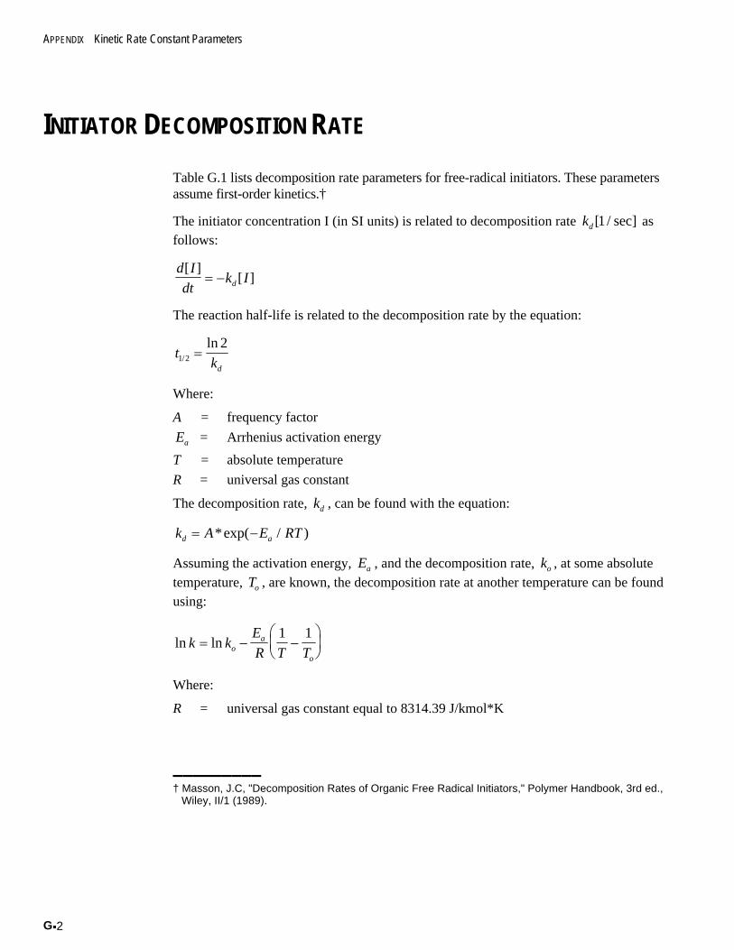
APPENDIX Kinetic Rate Constant Parameters
Gx2
INITIATOR DECOMPOSITION RATE
Table G.1 lists decomposition rate parameters for free-radical initiators. These parametersassume first-order kinetics.†
The initiator concentration I (in SI units) is related to decomposition rate kd[ / sec]1 asfollows:
d I
dtk Id
[ ][ ] �
The reaction half-life is related to the decomposition rate by the equation:
tkd
1 2
2/
ln
Where:
A = frequency factor
Ea = Arrhenius activation energy
T = absolute temperature
R = universal gas constant
The decomposition rate, kd , can be found with the equation:
k A E RTd a �*exp( / )
Assuming the activation energy, Ea , and the decomposition rate, ko , at some absolutetemperature, To , are known, the decomposition rate at another temperature can be foundusing:
ln lnk kE
R T Toa
o
� �§
©¨
·
¹¸
1 1
Where:
R = universal gas constant equal to 8314.39 J/kmol*K
_________† Masson, J.C, "Decomposition Rates of Organic Free Radical Initiators," Polymer Handbook, 3rd ed.,
Wiley, II/1 (1989).
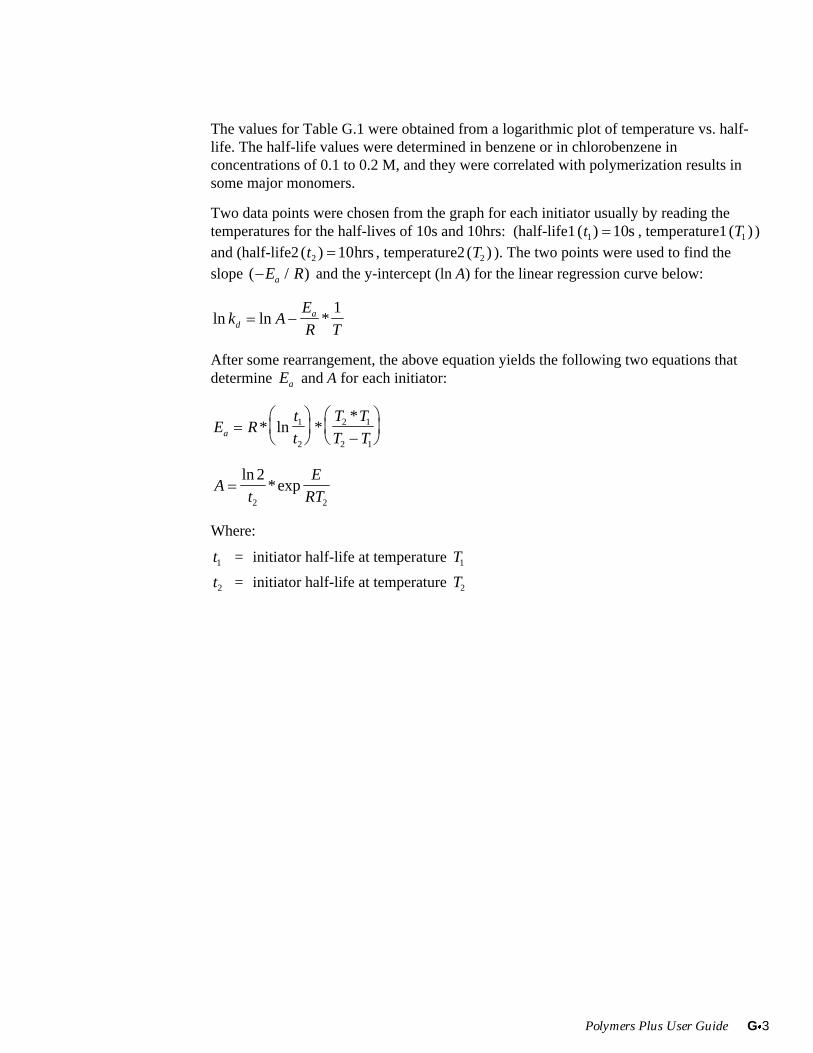
Polymers Plus User Guide Gx3
The values for Table G.1 were obtained from a logarithmic plot of temperature vs. half-life. The half-life values were determined in benzene or in chlorobenzene inconcentrations of 0.1 to 0.2 M, and they were correlated with polymerization results insome major monomers.
Two data points were chosen from the graph for each initiator usually by reading thetemperatures for the half-lives of 10s and 10hrs: (half-life1( )t1 10 s, temperature1( )T1 )and (half-life2( )t2 10 hrs, temperature2( )T2 ). The two points were used to find theslope ( / )�E Ra and the y-intercept (ln A) for the linear regression curve below:
ln ln *k AE
R Tda �
1
After some rearrangement, the above equation yields the following two equations thatdetermine Ea and A for each initiator:
E Rt
t
T T
T Ta §
©¨
·
¹¸
�
§
©¨
·
¹¸* ln *
*1
2
2 1
2 1
At
E
RT
ln*exp
2
2 2
Where:
t1 = initiator half-life at temperature T1
t2 = initiator half-life at temperature T2
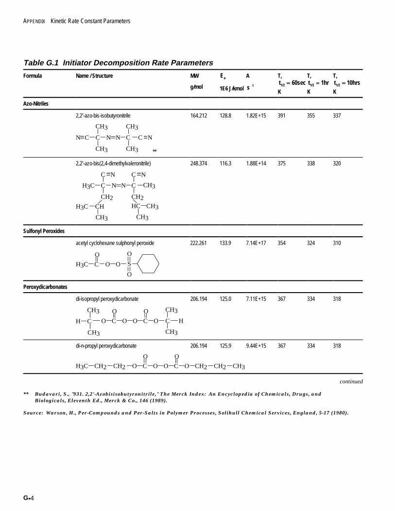
APPENDIX Kinetic Rate Constant Parameters
Gx4
Table G.1 Initiator Decomposition Rate Parameters
Formula Name / Structure MW
g/mol
Ea
1E6 J/kmol
A
s 1�
T,t 60sec1/2
K
T,t 1hr1/2
K
T,t 10hrs1/2
K
Azo-Nitriles
2,2'-azo-bis-isobutyronitrile 164.212 128.8 1.82E+15 391 355 337
C
CH3
NN
CH3
C
CH3
NCN C
CH3 **
2,2'-azo-bis(2,4-dimethylvaleronitrile) 248.374 116.3 1.88E+14 375 338 320
CH3CH
C
H3C
CH3
HC
NN
CH2
C CH3H3C
NCC N
CH2
CH3
Sulfonyl Peroxides
acetyl cyclohexane sulphonyl peroxide 222.261 133.9 7.14E+17 354 324 310
O O S
O
C
O
O
H3C
Peroxydicarbonates
di-isopropyl peroxydicarbonate 206.194 125.0 7.11E+15 367 334 318
OO C
OO
C OO
CH3
CH3
CH3
CH3
C HCH
di-n-propyl peroxydicarbonate 206.194 125.9 9.44E+15 367 334 318
CH3OO C
OO
C OOH3C CH2 CH2CH2 CH2
continued
** Budavari, S., "931. 2,2'-Azobisisobutyronitrile," The Merck Index: An Encyclopedia of Chemicals, Drugs, andBiologicals, Eleventh Ed., Merck & Co., 146 (1989).
Source: Warson, H., Per-Compounds and Per-Salts in Polymer Processes, Solihull Chemical Services, England, 5-17 (1980).
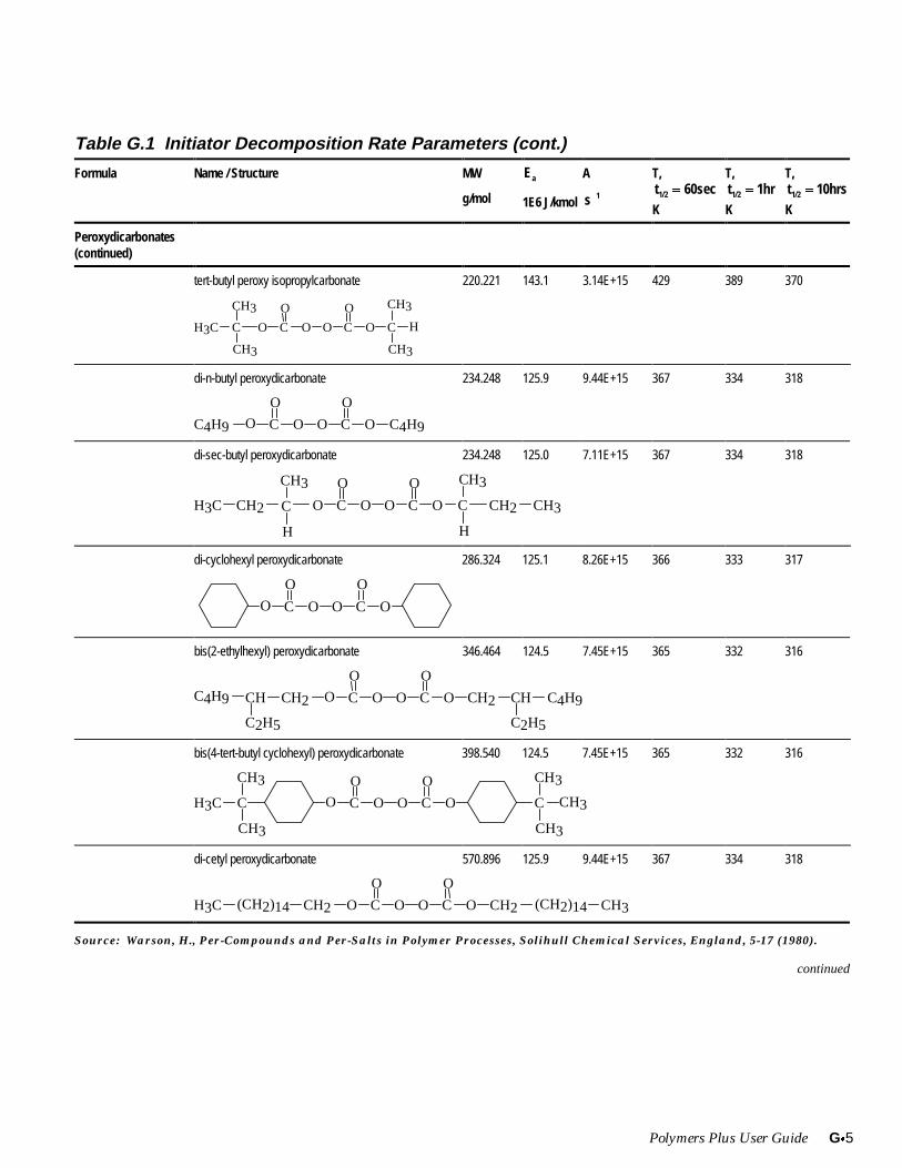
Polymers Plus User Guide Gx5
Table G.1 Initiator Decomposition Rate Parameters (cont.)
Formula Name / Structure MW
g/mol
Ea
1E6 J/kmol
A
s 1�
T,t 60sec1/2
K
T,t 1hr1/2
K
T,t 10hrs1/2
K
Peroxydicarbonates(continued)
tert-butyl peroxy isopropylcarbonate 220.221 143.1 3.14E+15 429 389 370
C
CH3
CH3C OO C
O
CH3
CH3 CH3
O HO
O
C
di-n-butyl peroxydicarbonate 234.248 125.9 9.44E+15 367 334 318
OO C
OO
C OOC4H9 C4H9
di-sec-butyl peroxydicarbonate 234.248 125.0 7.11E+15 367 334 318
COO C
OO
C OOH3C
H
CH3
CH2CH2 C CH3
H
CH3
di-cyclohexyl peroxydicarbonate 286.324 125.1 8.26E+15 366 333 317
OO C
OO
C OO
bis(2-ethylhexyl) peroxydicarbonate 346.464 124.5 7.45E+15 365 332 316
C2H5
CH2OO C
OO
C OO C4H9CH2 CHC4H9 CH
C2H5
bis(4-tert-butyl cyclohexyl) peroxydicarbonate 398.540 124.5 7.45E+15 365 332 316
C CH3H3C COO C
OO
C OO
CH3
CH3
CH3
CH3
di-cetyl peroxydicarbonate 570.896 125.9 9.44E+15 367 334 318
OO C
OO
C OOH3C (CH2)14 CH3CH2 CH2 (CH2)14
Source: Warson, H., Per-Compounds and Per-Salts in Polymer Processes, Solihull Chemical Services, England, 5-17 (1980).
continued
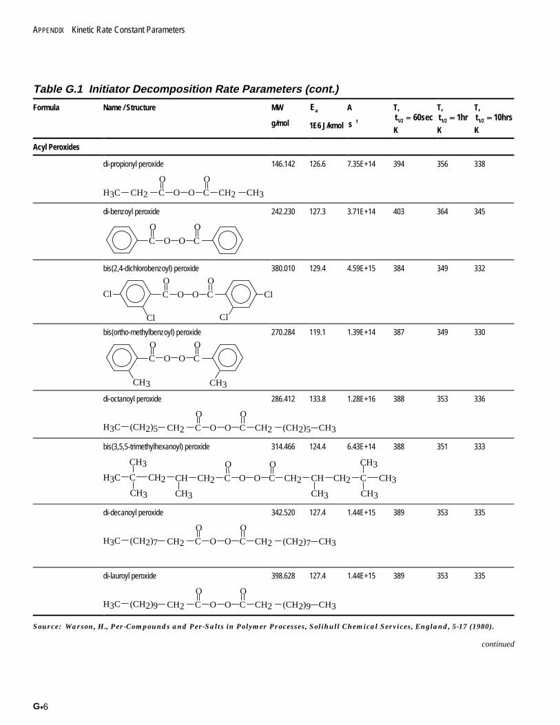
APPENDIX Kinetic Rate Constant Parameters
Gx6
Table G.1 Initiator Decomposition Rate Parameters (cont.)
Formula Name / Structure MW
g/mol
Ea
1E6 J/kmol
A
s 1�
T,t 60sec1/2
K
T,t 1hr1/2
K
T,t 10hrs1/2
K
Acyl Peroxides
di-propionyl peroxide 146.142 126.6 7.35E+14 394 356 338
CH3OO C
OO
CH3C CH2 CH2
di-benzoyl peroxide 242.230 127.3 3.71E+14 403 364 345
OO C
OO
C
bis(2,4-dichlorobenzoyl) peroxide 380.010 129.4 4.59E+15 384 349 332
Cl
OO C
OO
C
Cl
ClCl
bis(ortho-methylbenzoyl) peroxide 270.284 119.1 1.39E+14 387 349 330
OO C
OO
C
CH3 CH3
di-octanoyl peroxide 286.412 133.8 1.28E+16 388 353 336
CH3(CH2)5 OO C
OO
CH3C CH2 CH2 (CH2)5
bis(3,5,5-trimethylhexanoyl) peroxide 314.466 124.4 6.43E+14 388 351 333
C CH3
CH3
CHH3C OO C
OO
C
CH3
CH3
CH2
CH3
CH3
C CH2
CH3
CH CH2 CH2
di-decanoyl peroxide 342.520 127.4 1.44E+15 389 353 335
CH3(CH2)7 OO C
OO
CH3C CH2 CH2 (CH2)7
di-lauroyl peroxide 398.628 127.4 1.44E+15 389 353 335
CH3(CH2)9 OO C
OO
CH3C CH2 CH2 (CH2)9
Source: Warson, H., Per-Compounds and Per-Salts in Polymer Processes, Solihull Chemical Services, England, 5-17 (1980).
continued
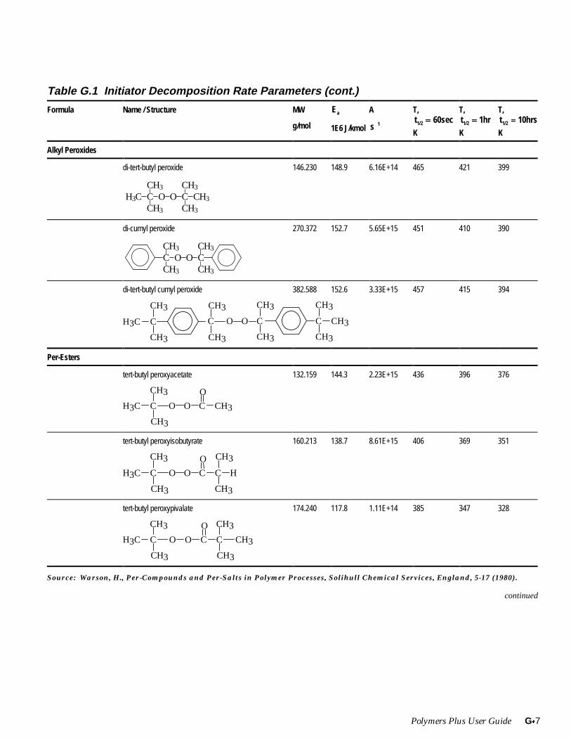
Polymers Plus User Guide Gx7
Table G.1 Initiator Decomposition Rate Parameters (cont.)
Formula Name / Structure MW
g/mol
Ea
1E6 J/kmol
A
s 1�
T,t 60sec1/2
K
T,t 1hr1/2
K
T,t 10hrs1/2
K
Alkyl Peroxides
di-tert-butyl peroxide 146.230 148.9 6.16E+14 465 421 399
H3C C O O C CH3
CH3
CH3
CH3
CH3
di-cumyl peroxide 270.372 152.7 5.65E+15 451 410 390
CH3
CH3
CH3
CH3
COOC
di-tert-butyl cumyl peroxide 382.588 152.6 3.33E+15 457 415 394
OO CC
CH3
CH3
CH3
CH3
H3C CH3
CH3
CH3
C
CH3
CH3
C
Per-Esters
tert-butyl peroxyacetate 132.159 144.3 2.23E+15 436 396 376
C CH3H3C OO C
O
CH3
CH3
tert-butyl peroxyisobutyrate 160.213 138.7 8.61E+15 406 369 351
C
CH3
CH3C OO C
O
CH3
CH3 CH3
H
tert-butyl peroxypivalate 174.240 117.8 1.11E+14 385 347 328
O OC CH3H3C
O
C
CH3
CH3 CH3
CH3
C
Source: Warson, H., Per-Compounds and Per-Salts in Polymer Processes, Solihull Chemical Services, England, 5-17 (1980).
continued
APPENDIX Kinetic Rate Constant Parameters
Gx8
Table G.1 Initiator Decomposition Rate Parameters (cont.)
Formula Name / Structure MW
g/mol
Ea
1E6 J/kmol
A
s 1�
T,t 60sec1/2
K
T,t 1hr1/2
K
T,t 10hrs1/2
K
Per-Esters (continued)
tert-butyl peroxydiethylacetate 188.267 126.7 2.07E+14 407 367 348
C
C2H5
CH3C OO C
O
CH3
CH3 C2H5
H
tert-butyl peroxybenzoate 194.230 138.8 2.96E+14 442 399 378
CH3C OO C
O
CH3
CH3
tert-butyl peroxy-2-ethylhexanoate 216.321 127.3 2.87E+14 406 366 347
C CH3
C2H5
CHH3C OO C
O
CH3
CH3
CH2 CH2 CH2
tert-butyl peroxy-3,5,5-trimethyl- hexanoate 230.348 143.0 2.38E+15 159 391 372
C CH3
CH3
CHH3C OO C
O
CH3
CH3
CH2 CH2 C
CH3
CH3
tert-butyl peroxyneodecanoate 244.375 121.3 1.26E+15 372 337 320
O OC CH3H3C
O
C
CH3
CH3
(CH2)5
CH3
CH3
C
Source: Warson, H., Per-Compounds and Per-Salts in Polymer Processes, Solihull Chemical Services, England, 5-17 (1980).
continued
Polymers Plus User Guide Gx9
Table G.1 Initiator Decomposition Rate Parameters (cont.)
Formula Name / Structure MW
g/mol
Ea
1E6 J/kmol
A
s 1�
T,t 60sec1/2
K
T,t 1hr1/2
K
T,t 10hrs1/2
K
Per-Ketals
2,2-di-tert-butyl peroxybutane 234.36 141.5 1.15E+15 435 394 374
C CH3H3C COO
CH3
CH3
CH3
CH3
O O
CH3
C
CH2
CH3
1,1-di-tert-butyl peroxycyclohexane 260.374 143.1 3.14E+15 429 389 370
C CH3H3C COO
CH3
CH3
CH3
CH3
O O
1,1-di-tert-butyl peroxy-3,5,5- trimethylcyclohexane 302.455 144.8 6.96E+15 426 387 368
C CH3H3C COO
CH3
CH3
CH3
CH3
O O
CH3
CH3
CH3
4,4-di-tert-butyl peroxy n-butyl valerate 334.453 139.5 2.10E+14 448 404 383
O O
CH3C O
O
CH3C C2H4
OO
C( CH3 )3
C( CH3 )3
CH2 CH2 CH2
1,4-bis(tert-butyl peroxyisopropyl) benzene 338.488 152.6 3.33E+15 457 415 394
OO CC
CH3
CH3
CH3
CH3
H3C
CH3
CH3
CH3
CH3
C CO O CH3
Source: Warson, H., Per-Compounds and Per-Salts in Polymer Processes, Solihull Chemical Services, England, 5-17 (1980).
continued
APPENDIX Kinetic Rate Constant Parameters
Gx10
Table G.1 Initiator Decomposition Rate Parameters (cont.)
Formula Name / Structure MW
g/mol
Ea
1E6 J/kmol
A
s 1�
T,t 60sec1/2
K
T,t 1hr1/2
K
T,t 10hrs1/2
K
Hydroperoxides
tert-butyl hydroperoxide 90.122 142.8 1.23E+12 532 472 444
OC
CH3
CH3
H3C HO
cumene hydroperoxide 152.193 113.0 9.05E+08 542 466 432
CH3
CH3
C O O H
di-isopropyl benzene monohydroperoxide 194.274 115.4 3.51E+09 525 455 423
CH3
CH3
CH C O O H
CH3
CH3
Source: Warson, H., Per-Compounds and Per-Salts in Polymer Processes, Solihull Chemical Services, England, 5-17 (1980).
Polymers Plus User Guide Hx1
H FORTRAN UTILITIES
This appendix describes the input and output arguments for various Fortran utilities usefulfor writing user kinetic subroutines. For each utility a list of variables in the argument listis given along with their I/O status, their type, and a brief description. These utilities areavailable to you in addition to those documented in the Aspen Plus User ModelsReference Manual.
The utilities documented in this appendix are:
x Component Attribute Handling Utilitiesx Component Handling Utilitiesx General Stream Handling Utilitiesx Other Utilities
A list of utilities contained in each category follows:
Component Attribute Handling Utilities
x CAELID (Hx3)x CAID (Hx4)x CAMIX (H x5)x CASPLT (Hx6)x CASPSS (Hx7)x CAUPDT (Hx8)x COPYCA (Hx9)x GETCRY (Hx10)x GETDPN (Hx11)x GETMWN (Hx12)x GETMWW (Hx13)x LCAOFF (Hx14)x LCATT (Hx15)x NCAVAR (Hx16)
H
APPENDIX Fortran Utilities for User Subroutines
Hx2
Component Handling Utilities
x CPACK (Hx17)x IFCMNC (Hx18)x ISCAT (Hx19)x ISOLIG (Hx20)x ISPOLY (Hx21)x ISSEG (Hx22)x SCPACK (Hx23)x XATOWT (Hx24)x XATOXT (H x25)
General Stream Handling Utilities
x IPTYPE (Hx26)x LOCATS (Hx27)x LPHASE (Hx28)x NPHASE (Hx29)x NSVAR (Hx30)x SSCOPY (Hx31)
Other Utilities
x VOLL (H x32)
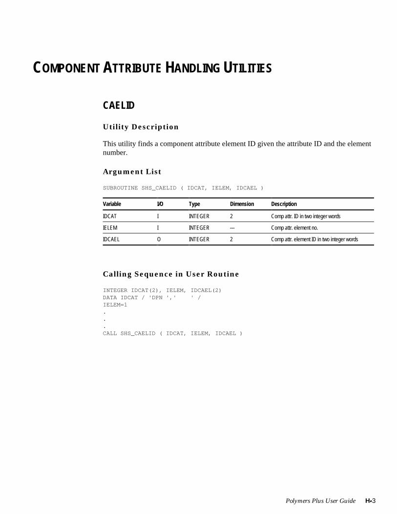
Polymers Plus User Guide Hx3
COMPONENT ATTRIBUTE HANDLING UTILITIES
CAELID
Utility Description
This utility finds a component attribute element ID given the attribute ID and the elementnumber.
Argument List
SUBROUTINE SHS_CAELID ( IDCAT, IELEM, IDCAEL )
Variable I/O Type Dimension Description
IDCAT I INTEGER 2 Comp attr. ID in two integer words
IELEM I INTEGER --- Comp attr. element no.
IDCAEL O INTEGER 2 Comp attr. element ID in two integer words
Calling Sequence in User Routine
INTEGER IDCAT(2), IELEM, IDCAEL(2)DATA IDCAT / 'DPN ',' ' /IELEM=1...CALL SHS_CAELID ( IDCAT, IELEM, IDCAEL )
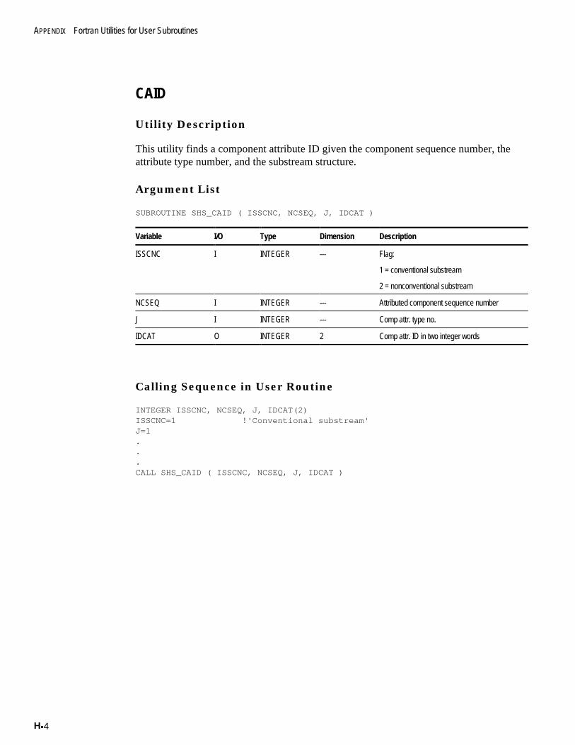
APPENDIX Fortran Utilities for User Subroutines
Hx4
CAID
Utility Description
This utility finds a component attribute ID given the component sequence number, theattribute type number, and the substream structure.
Argument List
SUBROUTINE SHS_CAID ( ISSCNC, NCSEQ, J, IDCAT )
Variable I/O Type Dimension Description
ISSCNC I INTEGER --- Flag:
1 = conventional substream
2 = nonconventional substream
NCSEQ I INTEGER --- Attributed component sequence number
J I INTEGER --- Comp attr. type no.
IDCAT O INTEGER 2 Comp attr. ID in two integer words
Calling Sequence in User Routine
INTEGER ISSCNC, NCSEQ, J, IDCAT(2)ISSCNC=1 !'Conventional substream'J=1...CALL SHS_CAID ( ISSCNC, NCSEQ, J, IDCAT )
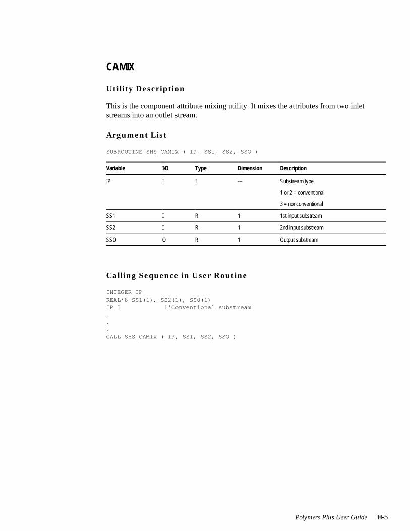
Polymers Plus User Guide Hx5
CAMIX
Utility Description
This is the component attribute mixing utility. It mixes the attributes from two inletstreams into an outlet stream.
Argument List
SUBROUTINE SHS_CAMIX ( IP, SS1, SS2, SSO )
Variable I/O Type Dimension Description
IP I I --- Substream type
1 or 2 = conventional
3 = nonconventional
SS1 I R 1 1st input substream
SS2 I R 1 2nd input substream
SSO O R 1 Output substream
Calling Sequence in User Routine
INTEGER IPREAL*8 SS1(1), SS2(1), SS0(1)IP=1 !'Conventional substream'...CALL SHS_CAMIX ( IP, SS1, SS2, SSO )
APPENDIX Fortran Utilities for User Subroutines
Hx6
CASPLT
Utility Description
This is the component attribute splitting utility. It calculates the attribute values in aproduct stream for a given feed stream.
Argument List
SUBROUTINE SHS_CASPLT ( FEED, PROD, NSUBS, IDXSUB, ITYPE )
Variable I/O Type Dimension Description
FEED I DBL (1) Combined feed stream
PROD O DBL (1) Given outlet stream
NSUBS I INT --- Number of substreams
ITYPE I INT NSUB Substream type vector
IDXSUB I INT NSUB Substream index vector
Calling Sequence in User Routine
INTEGER NSUBS, ITYPE(1), IDXSUB(1)REAL*8 FEED(1), PROD(1)IDXSUB(1)=1 !'First substream'ITYPE(1)=1 !'Conventional'...CALL SHS_CASPLT ( FEED, PROD, NSUBS, IDXSUB, ITYPE )
Polymers Plus User Guide Hx7
CASPSS
Utility Description
This is the component attribute splitting utility for substreams. It calculates the attributevalues in a product substream for a given feed substream.
Argument List
SUBROUTINE SHS_CASPSS ( FEED, PROD, ITYPE )
Variable I/O Type Dimension Description
FEED I DBL (1) Feed substream
PROD O DBL (1) Outlet substream
ITYPE I INT NSUB Substream type
Calling Sequence in User Routine
INTEGER ITYPE(1)REAL*8 FEED(1), PROD(1)ITYPE(1)=1 !'Conventional'...CALL SHS_CASPSS ( FEED, PROD, ITYPE )
APPENDIX Fortran Utilities for User Subroutines
Hx8
CAUPDT
Utility Description
This utility calculates class zero component attribute values in a product stream based onclass 2 component attributes.
Argument List
SUBROUTINE SHS_CAUPDT ( STREAM, NSUBS, IDXSUB, IPHASE )
Variable I/O Type Dimension Description
STREAM R*8 I (1) Stream vector
NSUBS I I --- Number of substreams
IDXSUB I I NSUBS Substream index vector
IPHASE I I NSUBS Substream type vector
1= MIXED
2= CISOLID
3= NCSOLID
Calling Sequence in User Routine
INTEGER NSUBS, IDXSUB(1), IPHASE(1)REAL*8 STREAM(1)IPHASE(1)=1 !'First phase'...CALL SHS_CAUPDT ( STREAM, NSUBS, IDXSUB, IPHASE )
Polymers Plus User Guide Hx9
COPYCA
Utility Description
This utility copies all attribute values from one stream into another stream of the sametype.
Argument List
SUBROUTINE SHS_COPYCA( LDIN, LD, LVRIN, LVR, IPHIN, IPH )
Variable I/O Type Dimension Description
LDIN I I --- Location of the descriptor bead for the inputstream
LD I I --- Location of the descriptor bead for the outputstream
LVRIN I I --- Location of the real stream variable data forthe input stream
LVR I I --- Location of the real stream variable
IPHIN I I --- Phase no. in the input stream
IPH I I --- Phase no. in the output stream data for theoutput stream
Calling Sequence in User Routine
INTEGER IPHIN, IPHINTEGE LDIN, LD, LVRIN, LVR !'Use LOCATS utility model to obtain these values'IPHIN=1IPH=1...CALL SHS_COPYCA( LDIN, LD, LVRIN, LVR, IPHIN, IPH )
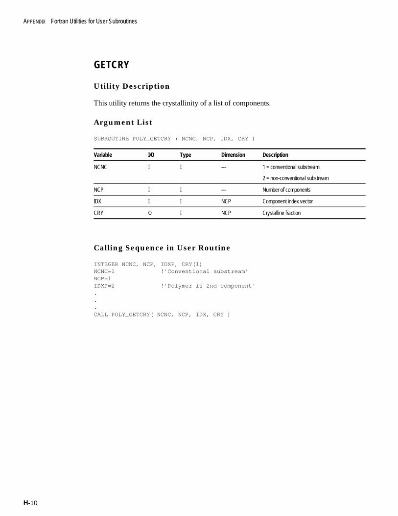
APPENDIX Fortran Utilities for User Subroutines
Hx10
GETCRY
Utility Description
This utility returns the crystallinity of a list of components.
Argument List
SUBROUTINE POLY_GETCRY ( NCNC, NCP, IDX, CRY )
Variable I/O Type Dimension Description
NCNC I I --- 1 = conventional substream
2 = non-conventional substream
NCP I I --- Number of components
IDX I I NCP Component index vector
CRY O I NCP Crystalline fraction
Calling Sequence in User Routine
INTEGER NCNC, NCP, IDXP, CRY(1)NCNC=1 !'Conventional substream'NCP=1IDXP=2 !'Polymer is 2nd component'...CALL POLY_GETCRY( NCNC, NCP, IDX, CRY )
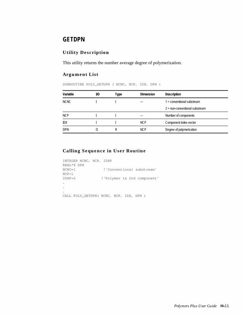
Polymers Plus User Guide Hx11
GETDPN
Utility Description
This utility returns the number average degree of polymerization.
Argument List
SUBROUTINE POLY_GETDPN ( NCNC, NCP, IDX, DPN )
Variable I/O Type Dimension Description
NCNC I I --- 1 = conventional substream
2 = non-conventional substream
NCP I I --- Number of components
IDX I I NCP Component index vector
DPN O R NCP Degree of polymerization
Calling Sequence in User Routine
INTEGER NCNC, NCP, IDXPREAL*8 DPNNCNC=1 !'Conventional substream'NCP=1IDXP=2 !'Polymer is 2nd component'...CALL POLY_GETDPN( NCNC, NCP, IDX, DPN )
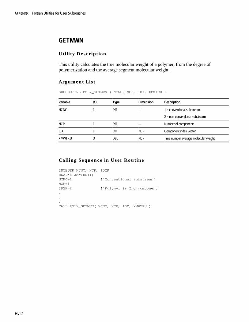
APPENDIX Fortran Utilities for User Subroutines
Hx12
GETMWN
Utility Description
This utility calculates the true molecular weight of a polymer, from the degree ofpolymerization and the average segment molecular weight.
Argument List
SUBROUTINE POLY_GETMWN ( NCNC, NCP, IDX, XMWTRU )
Variable I/O Type Dimension Description
NCNC I INT --- 1 = conventional substream
2 = non-conventional substream
NCP I INT --- Number of components
IDX I INT NCP Component index vector
XMWTRU O DBL NCP True number average molecular weight
Calling Sequence in User Routine
INTEGER NCNC, NCP, IDXPREAL*8 XMWTRU(1)NCNC=1 !'Conventional substream'NCP=1IDXP=2 !'Polymer is 2nd component'...CALL POLY_GETMWN( NCNC, NCP, IDX, XMWTRU )
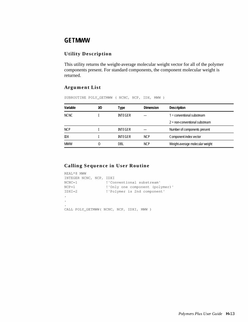
Polymers Plus User Guide Hx13
GETMWW
Utility Description
This utility returns the weight-average molecular weight vector for all of the polymercomponents present. For standard components, the component molecular weight isreturned.
Argument List
SUBROUTINE POLY_GETMWW ( NCNC, NCP, IDX, MWW )
Variable I/O Type Dimension Description
NCNC I INTEGER --- 1 = conventional substream
2 = non-conventional substream
NCP I INTEGER --- Number of components present
IDX I INTEGER NCP Component index vector
MWW O DBL NCP Weight-average molecular weight
Calling Sequence in User RoutineREAL*8 MWWINTEGER NCNC, NCP, IDXINCNC=1 !'Conventional substream'NCP=1 !'Only one component (polymer)'IDXI=2 !'Polymer is 2nd component'...CALL POLY_GETMWW( NCNC, NCP, IDXI, MWW )
APPENDIX Fortran Utilities for User Subroutines
Hx14
LCAOFF
Utility Description
This utility finds the offset of a component attribute from the beginning of the substreamgiven the structure of the substream, the component sequence number and the attributetype number.
Argument List
FUNCTION SHS_LCAOFF (ISSCNC, NCSEQ, J)
Variable I/O Type Dimension Description
ISSCNC I INTEGER --- Flag:
1 = Conventional substream
2 = non conventional substream
NCSEQ I INTEGER --- Attributed component sequence number
J I INTEGER --- Comp. attribute type no.
LCAOFF O INTEGER --- Attribute offset from substream
Calling Sequence in User Routine
INTEGER ISSCNC, NCSEQ, J, SHS_LCAOFFISSCNC=1 !'Conventional substream'NCSEQ=2 !'Second attributed component'J=1 !'First component attribute in the list for this component'...N = SHS_LCAOFF (ISSCNC, NCSEQ, J)
Polymers Plus User Guide Hx15
LCATT
Utility Description
This utility finds the offset of a component attribute from the substream given thestructure of the substream, attributed component sequence number and the attribute ID.
Argument List
FUNCTION SHS_LCATT (ISSCNC, NCSEQ, IDCATT)
Variable I/O Type Dimension Description
ISSCNC I INTEGER --- Flag:
1 = conventional substream
2 = non conventional substream
NCSEQ I INTEGER --- Attributed component sequence number
IDCATT I INTEGER 2 Component attribute ID in two integer words
LCATT O INTEGER --- Attribute offset
Calling Sequence in User Routine
INTEGER ISSCNC, NCSEQ, IAID(2), SHS_LCATTDATA IAD / DPN ', / ' ' /ISSCNC=1NCSEQ=1...N = SHS_LCATT (ISSCNC, NCSEQ, IAID)

APPENDIX Fortran Utilities for User Subroutines
Hx16
NCAVAR
Utility Description
This utility finds the number of elements in a component attribute given the attribute typeindex, the component index, and the substream type.
Argument List
FUNCTION SHS_NCAVAR (ISSCNC, NCSEQ, J)
Variable I/O Type Dimension Description
ISSCNC I INTEGER --- Flag:
1 = conventional substream
2 = non conventional substream
NCSEQ I INTEGER --- Attributed component sequence number
J I INTEGER --- Comp attribute type no.
NCAVAR O INTEGER --- Attribute length
Calling Sequence in User Routine
INTEGER ISSCNC, NCSEQ, J, SHS_NCAVARISSCNC=1 !'Conventional substream'NCSEQ=1J=1...N = SHS_NCAVAR (ISSCNC, NCSEQ, J)
Polymers Plus User Guide Hx17
COMPONENT HANDLING UTILITIES
CPACK
Utility Description
This utility packs a list of conventional components into an output vector which containscomponents whose mole fraction is greater than a minimun value XMIN.
Argument List
SUBROUTINE SHS_CPACK (PHASE, NCP, IDX, X, FLOW)
Variable I/O Type Dimension Description
PHASE I REAL NVCP Vector of component flows
NCP O INTEGER --- Number of components actually present
IDX O INTEGER NCC Index vector of components actually present
X O REAL NCC Mole fraction vector of components actuallypresent
FLOW O REAL --- Total molar flow of the phase
Calling Sequence in User Routine
INTEGER NCP, IDX(1)REAL*8 X(1), FLOW, PHASE(1)...CALL SHS_CPACK (PHASE, NCP, IDX, X, FLOW)
APPENDIX Fortran Utilities for User Subroutines
Hx18
IFCMNC
Utility Description
This utility is used to retrieve parameter values from the plex.
Argument List
FUNCTION DMS_IFCMNC ( NAME )
Variable I/O Type Dimension Description
NAME I CHARACTER*8 --- Parameter name as a character string
Calling Sequence in User Routine
C
INTEGER TC, I . . . TC(I)=DMS_IFCMNC('TC')+I
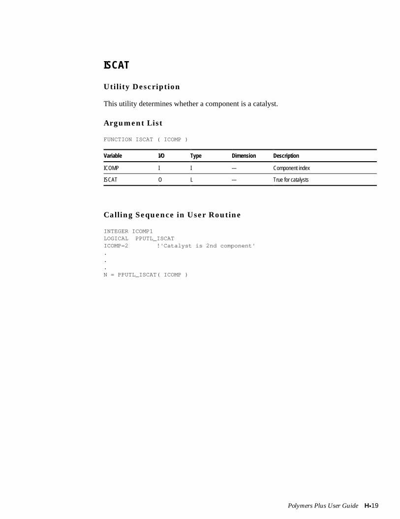
Polymers Plus User Guide Hx19
ISCAT
Utility Description
This utility determines whether a component is a catalyst.
Argument List
FUNCTION ISCAT ( ICOMP )
Variable I/O Type Dimension Description
ICOMP I I --- Component index
ISCAT O L --- True for catalysts
Calling Sequence in User Routine
INTEGER ICOMP1LOGICAL PPUTL_ISCATICOMP=2 !'Catalyst is 2nd component'...N = PPUTL_ISCAT( ICOMP )
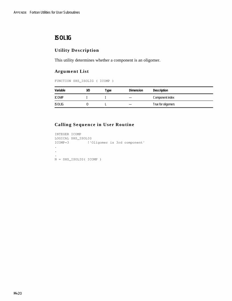
APPENDIX Fortran Utilities for User Subroutines
Hx20
ISOLIG
Utility Description
This utility determines whether a component is an oligomer.
Argument List
FUNCTION SHS_ISOLIG ( ICOMP )
Variable I/O Type Dimension Description
ICOMP I I --- Component index
ISOLIG O L --- True for oligomers
Calling Sequence in User Routine
INTEGER ICOMPLOGICAL SHS_ISOLIGICOMP=3 !'Oligomer is 3rd component'...N = SHS_ISOLIG( ICOMP )
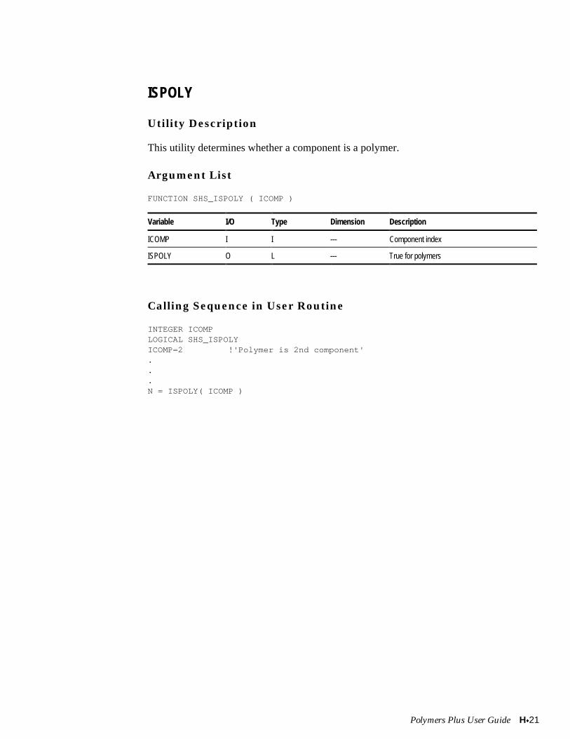
Polymers Plus User Guide Hx21
ISPOLY
Utility Description
This utility determines whether a component is a polymer.
Argument List
FUNCTION SHS_ISPOLY ( ICOMP )
Variable I/O Type Dimension Description
ICOMP I I --- Component index
ISPOLY O L --- True for polymers
Calling Sequence in User Routine
INTEGER ICOMPLOGICAL SHS_ISPOLYICOMP=2 !'Polymer is 2nd component'...N = ISPOLY( ICOMP )

APPENDIX Fortran Utilities for User Subroutines
Hx22
ISSEG
Utility Description
This utility determines whether a component is a segment.
Argument List
FUNCTION PPUTL_ISSEG ( ICOMP )
Variable I/O Type Dimension Description
ICOMP I I --- Component index
ISSEG O L --- True for segments
Calling Sequence in User Routine
INTEGER ICOMPLOGICAL PPUTL_ISSEGICOMP=5 !'Segment is 5th component'...N = PPUTL_ISSEG( ICOMP )
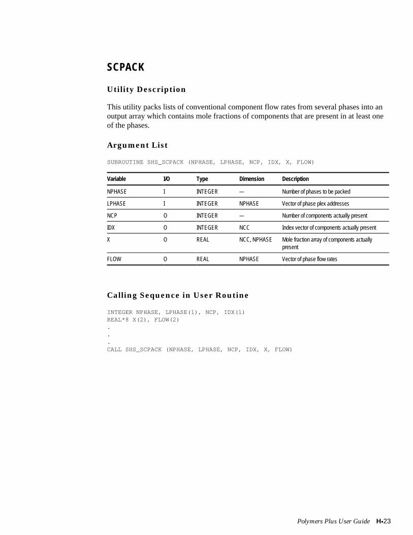
Polymers Plus User Guide Hx23
SCPACK
Utility Description
This utility packs lists of conventional component flow rates from several phases into anoutput array which contains mole fractions of components that are present in at least oneof the phases.
Argument List
SUBROUTINE SHS_SCPACK (NPHASE, LPHASE, NCP, IDX, X, FLOW)
Variable I/O Type Dimension Description
NPHASE I INTEGER --- Number of phases to be packed
LPHASE I INTEGER NPHASE Vector of phase plex addresses
NCP O INTEGER --- Number of components actually present
IDX O INTEGER NCC Index vector of components actually present
X O REAL NCC, NPHASE Mole fraction array of components actuallypresent
FLOW O REAL NPHASE Vector of phase flow rates
Calling Sequence in User Routine
INTEGER NPHASE, LPHASE(1), NCP, IDX(1)REAL*8 X(2), FLOW(2)...CALL SHS_SCPACK (NPHASE, LPHASE, NCP, IDX, X, FLOW)
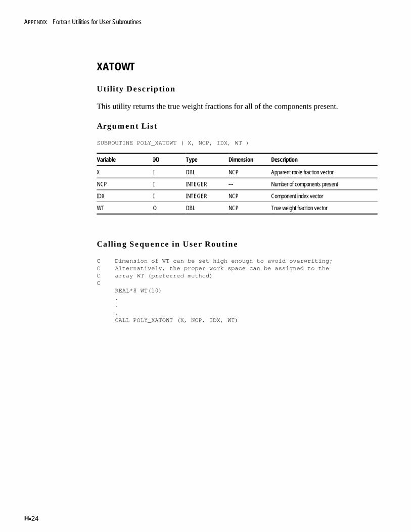
APPENDIX Fortran Utilities for User Subroutines
Hx24
XATOWT
Utility Description
This utility returns the true weight fractions for all of the components present.
Argument List
SUBROUTINE POLY_XATOWT ( X, NCP, IDX, WT )
Variable I/O Type Dimension Description
X I DBL NCP Apparent mole fraction vector
NCP I INTEGER --- Number of components present
IDX I INTEGER NCP Component index vector
WT O DBL NCP True weight fraction vector
Calling Sequence in User Routine
C Dimension of WT can be set high enough to avoid overwriting;C Alternatively, the proper work space can be assigned to theC array WT (preferred method)C REAL*8 WT(10) . . . CALL POLY_XATOWT (X, NCP, IDX, WT)
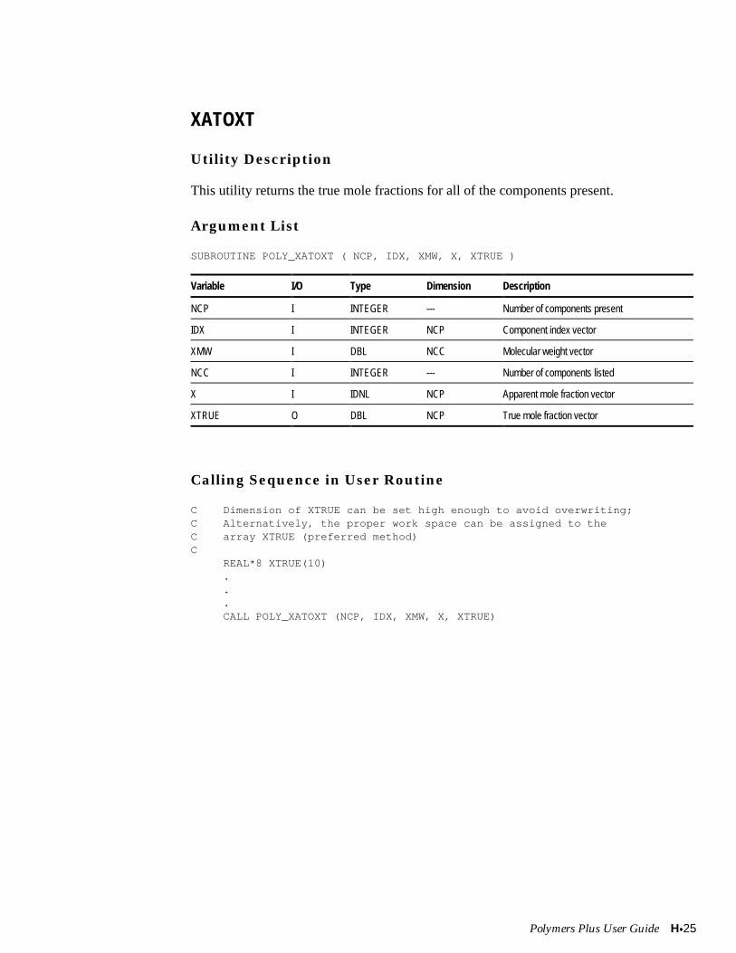
Polymers Plus User Guide Hx25
XATOXT
Utility Description
This utility returns the true mole fractions for all of the components present.
Argument List
SUBROUTINE POLY_XATOXT ( NCP, IDX, XMW, X, XTRUE )
Variable I/O Type Dimension Description
NCP I INTEGER --- Number of components present
IDX I INTEGER NCP Component index vector
XMW I DBL NCC Molecular weight vector
NCC I INTEGER --- Number of components listed
X I IDNL NCP Apparent mole fraction vector
XTRUE O DBL NCP True mole fraction vector
Calling Sequence in User Routine
C Dimension of XTRUE can be set high enough to avoid overwriting;C Alternatively, the proper work space can be assigned to theC array XTRUE (preferred method)C REAL*8 XTRUE(10) . . . CALL POLY_XATOXT (NCP, IDX, XMW, X, XTRUE)
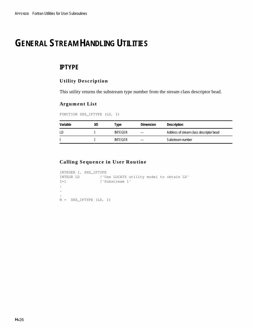
APPENDIX Fortran Utilities for User Subroutines
Hx26
GENERAL STREAM HANDLING UTILITIES
IPTYPE
Utility Description
This utility returns the substream type number from the stream class descriptor bead.
Argument List
FUNCTION SHS_IPTYPE (LD, I)
Variable I/O Type Dimension Description
LD I INTEGER --- Address of stream class descriptor bead
I I INTEGER --- Substream number
Calling Sequence in User Routine
INTEGER I, SHS_IPTYPEINTEGR LD !'Use LOCATS utility model to obtain LD'I=1 !'Substream 1'...N = SHS_IPTYPE (LD, I)
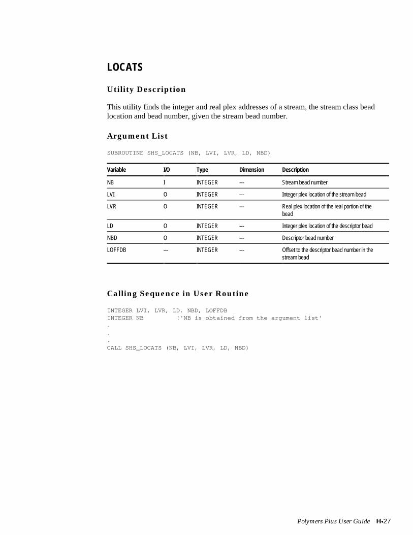
Polymers Plus User Guide Hx27
LOCATS
Utility Description
This utility finds the integer and real plex addresses of a stream, the stream class beadlocation and bead number, given the stream bead number.
Argument List
SUBROUTINE SHS_LOCATS (NB, LVI, LVR, LD, NBD)
Variable I/O Type Dimension Description
NB I INTEGER --- Stream bead number
LVI O INTEGER --- Integer plex location of the stream bead
LVR O INTEGER --- Real plex location of the real portion of thebead
LD O INTEGER --- Integer plex location of the descriptor bead
NBD O INTEGER --- Descriptor bead number
LOFFDB --- INTEGER --- Offset to the descriptor bead number in thestream bead
Calling Sequence in User Routine
INTEGER LVI, LVR, LD, NBD, LOFFDBINTEGER NB !'NB is obtained from the argument list'...CALL SHS_LOCATS (NB, LVI, LVR, LD, NBD)
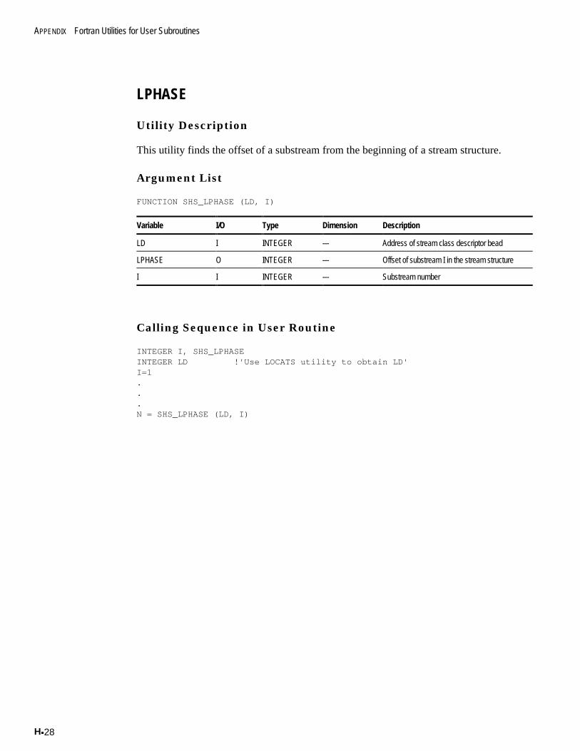
APPENDIX Fortran Utilities for User Subroutines
Hx28
LPHASE
Utility Description
This utility finds the offset of a substream from the beginning of a stream structure.
Argument List
FUNCTION SHS_LPHASE (LD, I)
Variable I/O Type Dimension Description
LD I INTEGER --- Address of stream class descriptor bead
LPHASE O INTEGER --- Offset of substream I in the stream structure
I I INTEGER --- Substream number
Calling Sequence in User Routine
INTEGER I, SHS_LPHASEINTEGER LD !'Use LOCATS utility to obtain LD'I=1...N = SHS_LPHASE (LD, I)
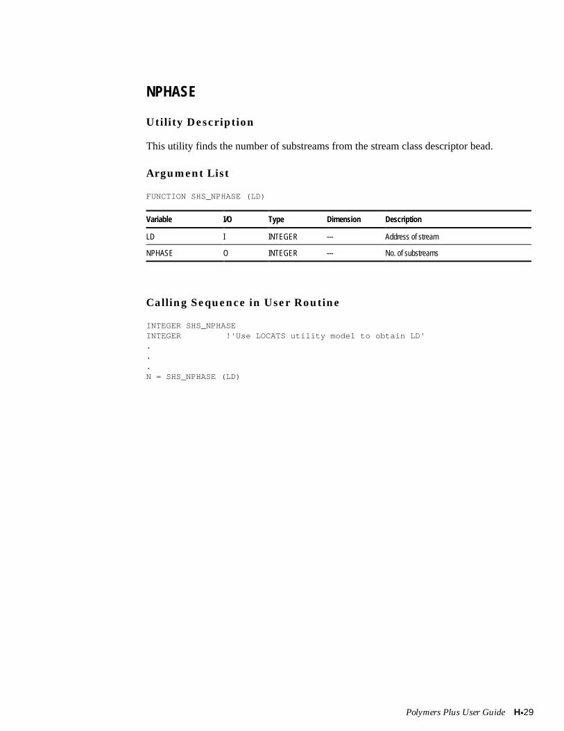
Polymers Plus User Guide Hx29
NPHASE
Utility Description
This utility finds the number of substreams from the stream class descriptor bead.
Argument List
FUNCTION SHS_NPHASE (LD)
Variable I/O Type Dimension Description
LD I INTEGER --- Address of stream
NPHASE O INTEGER --- No. of substreams
Calling Sequence in User Routine
INTEGER SHS_NPHASEINTEGER !'Use LOCATS utility model to obtain LD'...N = SHS_NPHASE (LD)
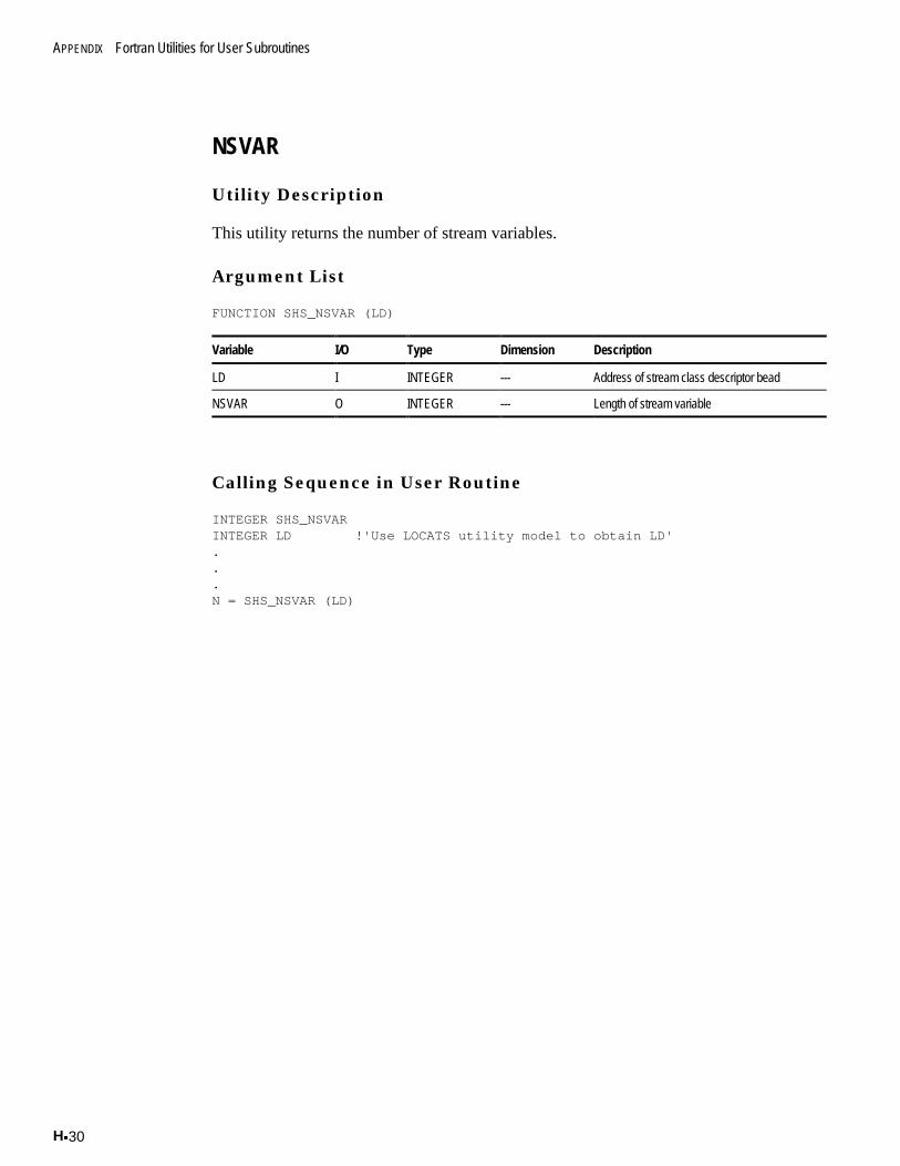
APPENDIX Fortran Utilities for User Subroutines
Hx30
NSVAR
Utility Description
This utility returns the number of stream variables.
Argument List
FUNCTION SHS_NSVAR (LD)
Variable I/O Type Dimension Description
LD I INTEGER --- Address of stream class descriptor bead
NSVAR O INTEGER --- Length of stream variable
Calling Sequence in User Routine
INTEGER SHS_NSVARINTEGER LD !'Use LOCATS utility model to obtain LD'...N = SHS_NSVAR (LD)
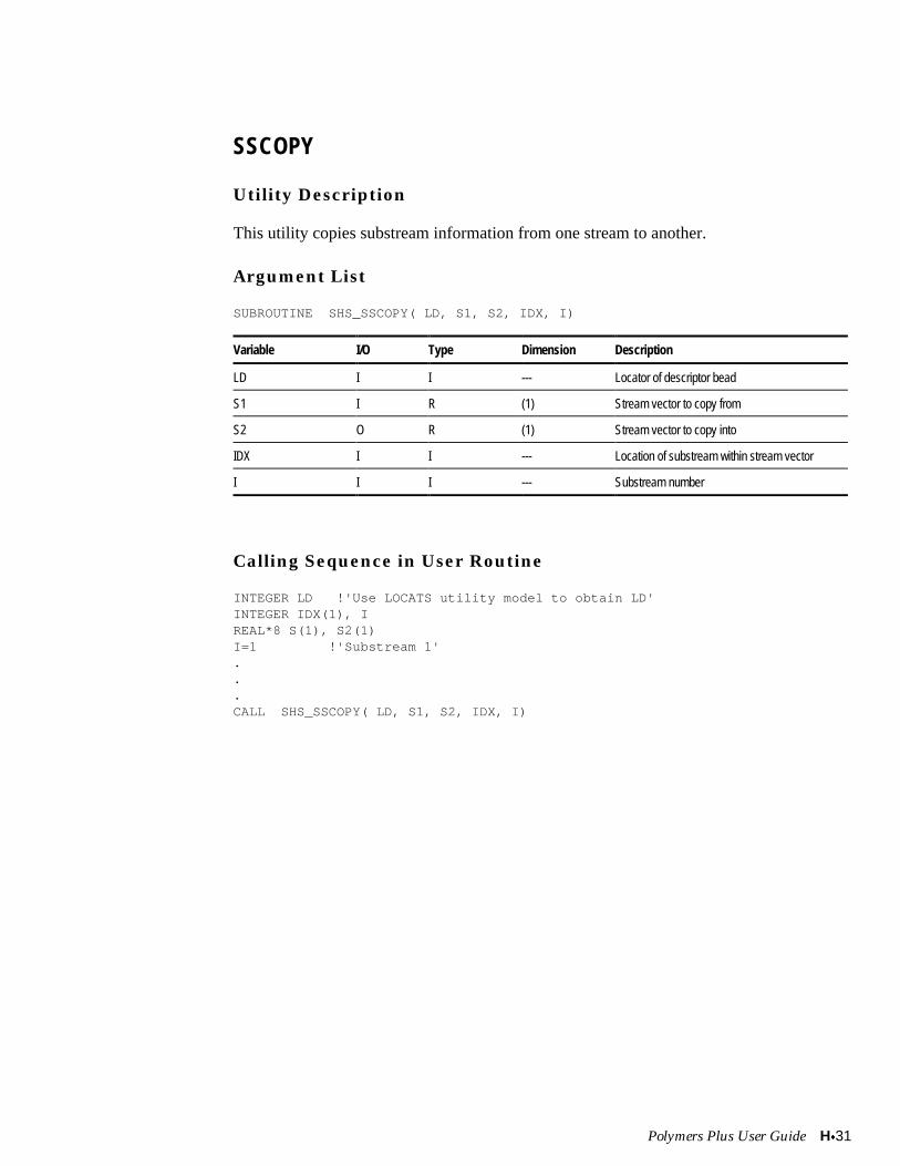
Polymers Plus User Guide Hx31
SSCOPY
Utility Description
This utility copies substream information from one stream to another.
Argument List
SUBROUTINE SHS_SSCOPY( LD, S1, S2, IDX, I)
Variable I/O Type Dimension Description
LD I I --- Locator of descriptor bead
S1 I R (1) Stream vector to copy from
S2 O R (1) Stream vector to copy into
IDX I I --- Location of substream within stream vector
I I I --- Substream number
Calling Sequence in User Routine
INTEGER LD !'Use LOCATS utility model to obtain LD'INTEGER IDX(1), IREAL*8 S(1), S2(1)I=1 !'Substream 1'...CALL SHS_SSCOPY( LD, S1, S2, IDX, I)
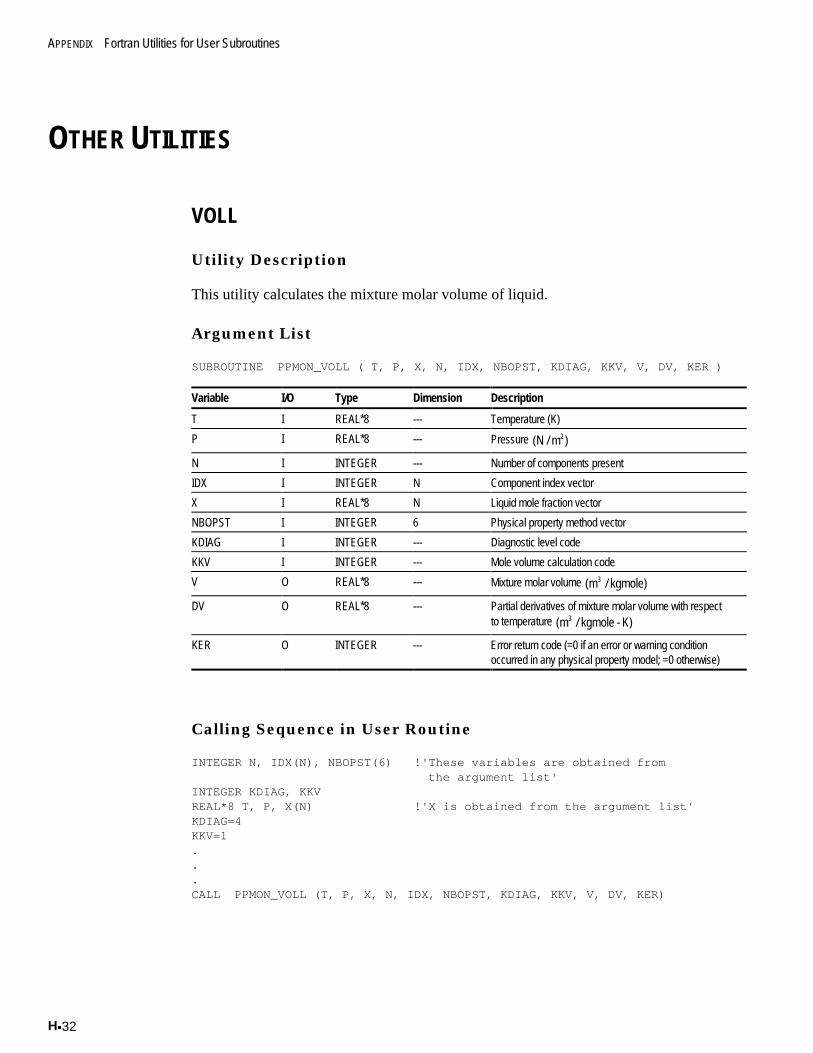
APPENDIX Fortran Utilities for User Subroutines
Hx32
OTHER UTILITIES
VOLL
Utility Description
This utility calculates the mixture molar volume of liquid.
Argument List
SUBROUTINE PPMON_VOLL ( T, P, X, N, IDX, NBOPST, KDIAG, KKV, V, DV, KER )
Variable I/O Type Dimension Description
T I REAL*8 --- Temperature (K)
P I REAL*8 --- Pressure (N / m )2
N I INTEGER --- Number of components present
IDX I INTEGER N Component index vector
X I REAL*8 N Liquid mole fraction vector
NBOPST I INTEGER 6 Physical property method vector
KDIAG I INTEGER --- Diagnostic level code
KKV I INTEGER --- Mole volume calculation code
V O REAL*8 --- Mixture molar volume (m / kgmole)3
DV O REAL*8 --- Partial derivatives of mixture molar volume with respectto temperature (m / kgmole - K)3
KER O INTEGER --- Error return code (=0 if an error or warning conditionoccurred in any physical property model; =0 otherwise)
Calling Sequence in User Routine
INTEGER N, IDX(N), NBOPST(6) !'These variables are obtained from the argument list'INTEGER KDIAG, KKVREAL*8 T, P, X(N) !'X is obtained from the argument list'KDIAG=4KKV=1...CALL PPMON_VOLL (T, P, X, N, IDX, NBOPST, KDIAG, KKV, V, DV, KER)
POLYMERS PLUS User Guide Input x1
INPUT LANGUAGE REFERENCE
This section describes the input language for:
x Specifying Components (Inputx2)x Specifying Component Attributes (Inputx5)x Requesting Distribution Calculations (Inputx7)x Calculating End Use Properties (Inputx8)x Specifying Physical Property Inputs (Inputx10)x Specifying Step-Growth Polymerization Kinetics (Inputx15)x Specifying Free-Radical Polymerization Kinetics (Inputx22)x Specifying Emulsion Polymerization Kinetics (Inputx30)x Specifying Ziegler-Natta Polymerization Kinetics (Inputx38)x Specifying Ionic Polymerization Kinetics (Inputx50)x Specifying Segment-Based Polymer Modification Reactions (Inputx58)
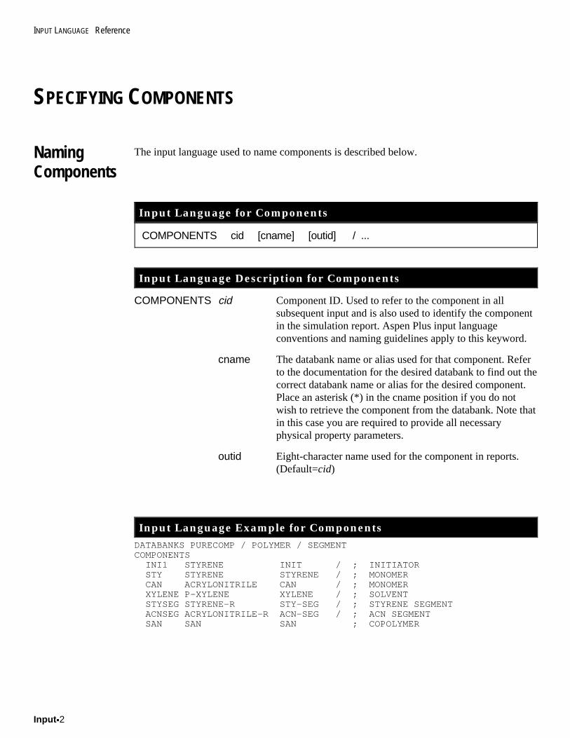
INPUT LANGUAGE Reference
Input x2
SPECIFYING COMPONENTS
NamingComponents
The input language used to name components is described below.
Input Language for Components
COMPONENTS cid [cname] [outid] / ...
Input Language Description for Components
COMPONENTS cid Component ID. Used to refer to the component in allsubsequent input and is also used to identify the componentin the simulation report. Aspen Plus input languageconventions and naming guidelines apply to this keyword.
cname The databank name or alias used for that component. Referto the documentation for the desired databank to find out thecorrect databank name or alias for the desired component.Place an asterisk (*) in the cname position if you do notwish to retrieve the component from the databank. Note thatin this case you are required to provide all necessaryphysical property parameters.
outid Eight-character name used for the component in reports.(Default=cid)
Input Language Example for ComponentsDATABANKS PURECOMP / POLYMER / SEGMENTCOMPONENTS INI1 STYRENE INIT / ; INITIATOR STY STYRENE STYRENE / ; MONOMER CAN ACRYLONITRILE CAN / ; MONOMER XYLENE P-XYLENE XYLENE / ; SOLVENT STYSEG STYRENE-R STY-SEG / ; STYRENE SEGMENT ACNSEG ACRYLONITRILE-R ACN-SEG / ; ACN SEGMENT SAN SAN SAN ; COPOLYMER
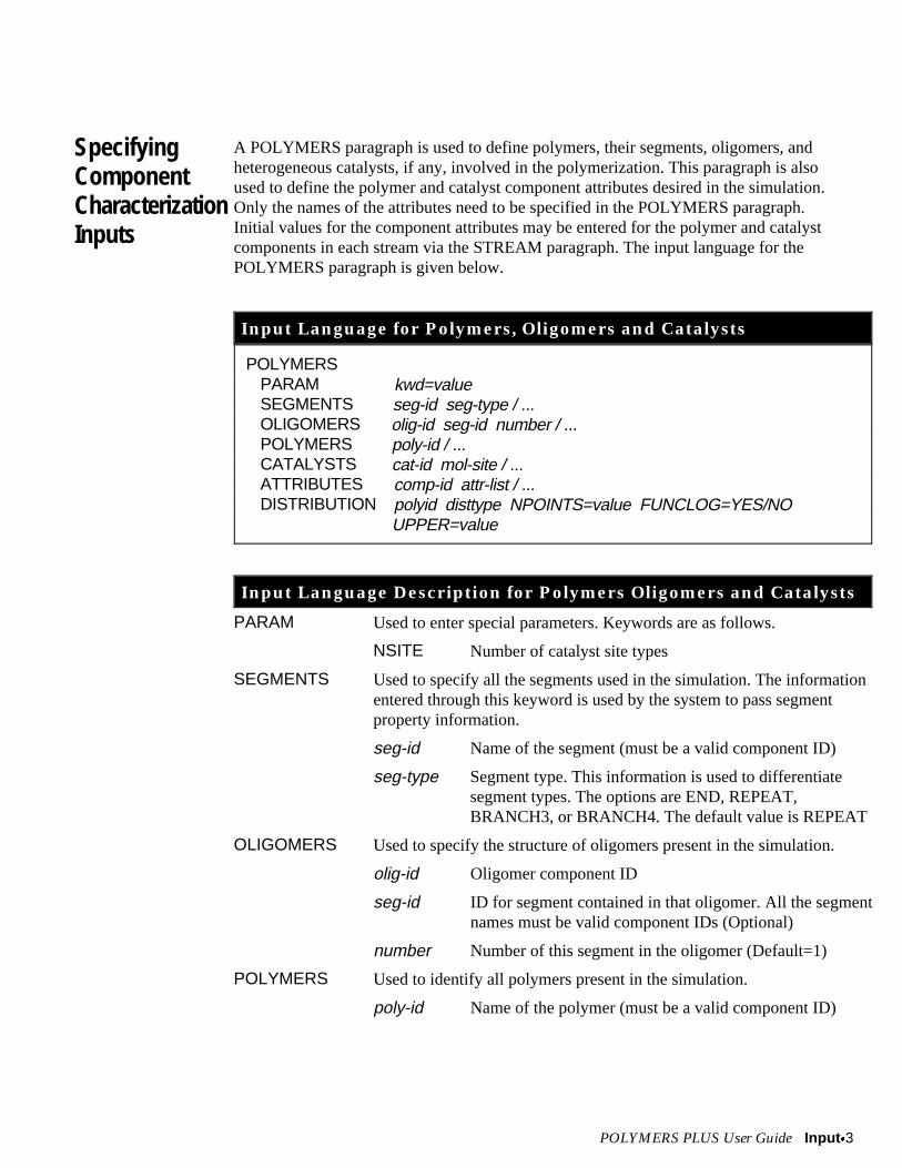
POLYMERS PLUS User Guide Input x3
SpecifyingComponentCharacterizationInputs
A POLYMERS paragraph is used to define polymers, their segments, oligomers, andheterogeneous catalysts, if any, involved in the polymerization. This paragraph is alsoused to define the polymer and catalyst component attributes desired in the simulation.Only the names of the attributes need to be specified in the POLYMERS paragraph.Initial values for the component attributes may be entered for the polymer and catalystcomponents in each stream via the STREAM paragraph. The input language for thePOLYMERS paragraph is given below.
Input Language for Polymers, Oligomers and Catalysts
POLYMERSPARAM kwd=valueSEGMENTS seg-id seg-type / ...OLIGOMERS olig-id seg-id number / ...POLYMERS poly-id / ...CATALYSTS cat-id mol-site / ...ATTRIBUTES comp-id attr-list / ...DISTRIBUTION polyid disttype NPOINTS=value FUNCLOG=YES/NO
UPPER=value
Input Language Description for Polymers Oligomers and Catalysts
PARAM Used to enter special parameters. Keywords are as follows.
NSITE Number of catalyst site types
SEGMENTS Used to specify all the segments used in the simulation. The informationentered through this keyword is used by the system to pass segmentproperty information.
seg-id Name of the segment (must be a valid component ID)
seg-type Segment type. This information is used to differentiatesegment types. The options are END, REPEAT,BRANCH3, or BRANCH4. The default value is REPEAT
OLIGOMERS Used to specify the structure of oligomers present in the simulation.
olig-id Oligomer component ID
seg-id ID for segment contained in that oligomer. All the segmentnames must be valid component IDs (Optional)
number Number of this segment in the oligomer (Default=1)
POLYMERS Used to identify all polymers present in the simulation.
poly-id Name of the polymer (must be a valid component ID)
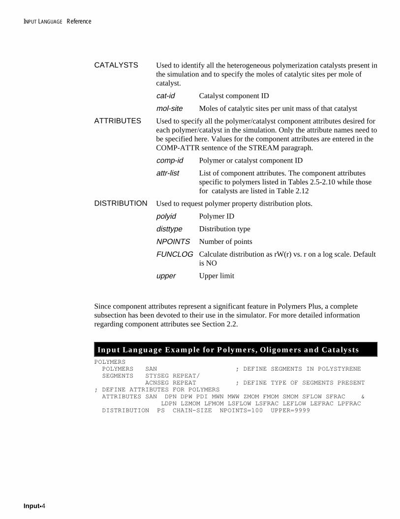
INPUT LANGUAGE Reference
Input x4
CATALYSTS Used to identify all the heterogeneous polymerization catalysts present inthe simulation and to specify the moles of catalytic sites per mole ofcatalyst.
cat-id Catalyst component ID
mol-site Moles of catalytic sites per unit mass of that catalyst
ATTRIBUTES Used to specify all the polymer/catalyst component attributes desired foreach polymer/catalyst in the simulation. Only the attribute names need tobe specified here. Values for the component attributes are entered in theCOMP-ATTR sentence of the STREAM paragraph.
comp-id Polymer or catalyst component ID
attr-list List of component attributes. The component attributesspecific to polymers listed in Tables 2.5-2.10 while thosefor catalysts are listed in Table 2.12
DISTRIBUTION Used to request polymer property distribution plots.
polyid Polymer ID
disttype Distribution type
NPOINTS Number of points
FUNCLOG Calculate distribution as rW(r) vs. r on a log scale. Defaultis NO
upper Upper limit
Since component attributes represent a significant feature in Polymers Plus, a completesubsection has been devoted to their use in the simulator. For more detailed informationregarding component attributes see Section 2.2.
Input Language Example for Polymers, Oligomers and CatalystsPOLYMERS POLYMERS SAN ; DEFINE SEGMENTS IN POLYSTYRENE SEGMENTS STYSEG REPEAT/ ACNSEG REPEAT ; DEFINE TYPE OF SEGMENTS PRESENT; DEFINE ATTRIBUTES FOR POLYMERS ATTRIBUTES SAN DPN DPW PDI MWN MWW ZMOM FMOM SMOM SFLOW SFRAC & LDPN LZMOM LFMOM LSFLOW LSFRAC LEFLOW LEFRAC LPFRAC DISTRIBUTION PS CHAIN-SIZE NPOINTS=100 UPPER=9999
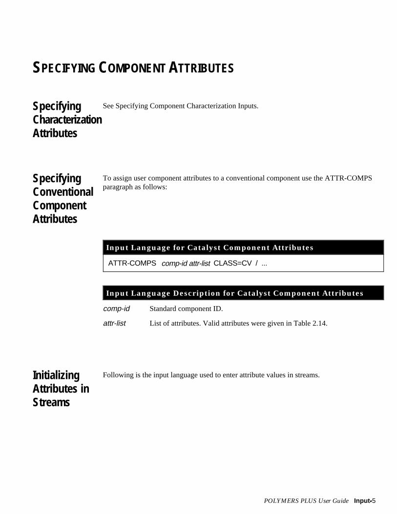
POLYMERS PLUS User Guide Input x5
SPECIFYING COMPONENT ATTRIBUTES
SpecifyingCharacterizationAttributes
See Specifying Component Characterization Inputs.
SpecifyingConventionalComponentAttributes
To assign user component attributes to a conventional component use the ATTR-COMPSparagraph as follows:
Input Language for Catalyst Component Attributes
ATTR-COMPS comp-id attr-list CLASS=CV / ...
Input Language Description for Catalyst Component Attributes
comp-id Standard component ID.
attr-list List of attributes. Valid attributes were given in Table 2.14.
InitializingAttributes inStreams
Following is the input language used to enter attribute values in streams.
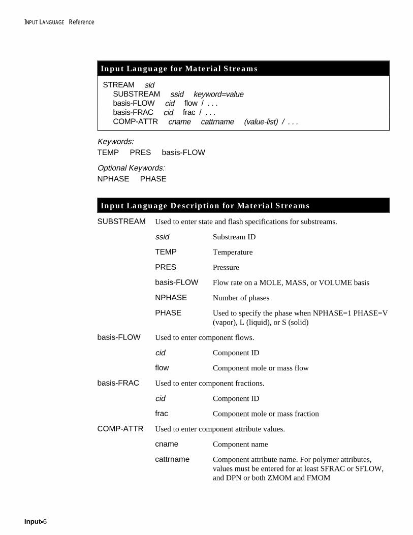
INPUT LANGUAGE Reference
Input x6
Input Language for Material Streams
STREAM sid SUBSTREAM ssid keyword=value basis-FLOW cid flow / . . . basis-FRAC cid frac / . . . COMP-ATTR cname cattrname (value-list) / . . .
Keywords:TEMP PRES basis-FLOW
Optional Keywords:NPHASE PHASE
Input Language Description for Material Streams
SUBSTREAM Used to enter state and flash specifications for substreams.
ssid Substream ID
TEMP Temperature
PRES Pressure
basis-FLOW Flow rate on a MOLE, MASS, or VOLUME basis
NPHASE Number of phases
PHASE Used to specify the phase when NPHASE=1 PHASE=V(vapor), L (liquid), or S (solid)
basis-FLOW Used to enter component flows.
cid Component ID
flow Component mole or mass flow
basis-FRAC Used to enter component fractions.
cid Component ID
frac Component mole or mass fraction
COMP-ATTR Used to enter component attribute values.
cname Component name
cattrname Component attribute name. For polymer attributes,values must be entered for at least SFRAC or SFLOW,and DPN or both ZMOM and FMOM
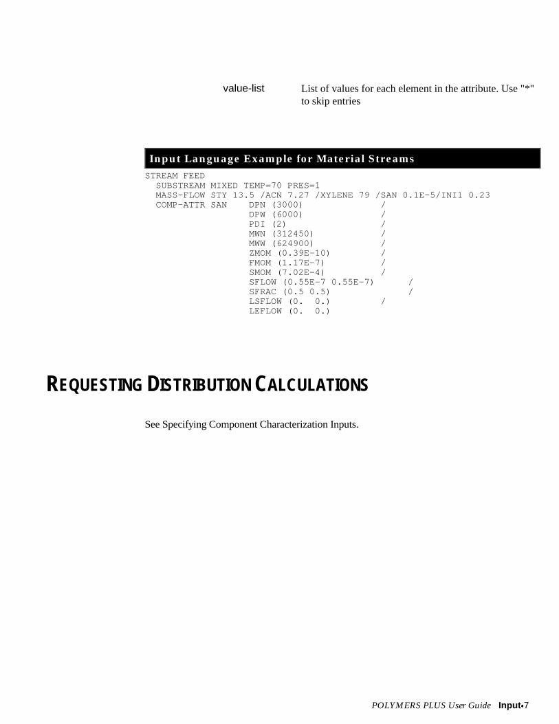
POLYMERS PLUS User Guide Input x7
value-list List of values for each element in the attribute. Use "*"to skip entries
Input Language Example for Material StreamsSTREAM FEED SUBSTREAM MIXED TEMP=70 PRES=1 MASS-FLOW STY 13.5 /ACN 7.27 /XYLENE 79 /SAN 0.1E-5/INI1 0.23 COMP-ATTR SAN DPN (3000) / DPW (6000) / PDI (2) / MWN (312450) / MWW (624900) / ZMOM (0.39E-10) / FMOM (1.17E-7) / SMOM (7.02E-4) / SFLOW (0.55E-7 0.55E-7) / SFRAC (0.5 0.5) / LSFLOW (0. 0.) / LEFLOW (0. 0.)
REQUESTING DISTRIBUTION CALCULATIONS
See Specifying Component Characterization Inputs.
INPUT LANGUAGE Reference
Input x8
CALCULATING END USE PROPERTIES
Input Language for Prop-Set
PROP-SET propsetid propname-list keyword=value
Optional Keywords:COMPS PHASE UNITS TEMP PRES
Input Language Description for Prop-Set
Use the Prop-Set paragraph to define a property set. A property set is a collection ofthermodynamic, transport, and other properties. Each property set you define is identifiedby an ID you supply.
propsetid Property set ID.
propname-list List of property names. (See Aspen Plus Physical Property DataReference Manual.)
COMPS List of component IDs (applies to all properties listed in Aspen PlusPhysical Property Data Reference Manual). (Default=all componentsactually present when the property is calculated.)
PHASE PHASE=V Vapor
PHASE=L Total liquid
PHASE=L1 First-liquid
PHASE=L2 Second-liquid
PHASE=T Total mixture
PHASE=S Solid
Phase compositions are determined at stream conditions. (Default=T, iflisted as a valid phase for the property in Aspen Plus Physical PropertyData Reference Manual; otherwise no default.)
UNITS Units options selected for the units keywords that are listed for theproperty in Aspen Plus Physical Property Data Reference Manual.(Default=IN-UNITS if Prop-Set is specified for design specifications,Fortran blocks, optimization paragraphs and constraint paragraphs.Default=OUT-UNITS if Prop-Set is specified for reports. If a property hasmole, mass, or flow units, the default will be mole units.)
POLYMERS PLUS User Guide Input x9
TEMP Temperatures for property calculations. (Default=stream temperature. ForVVSTD and VVSTDMX, Default=25qC.)
PRES Pressures for property calculations. (Default=stream pressure. For VVSTDand VVSTDMX, Default=1 atm.)
Input Language for USER-PROPERTY
USER-PROPERTY userpropid propname-list keyword=value
Keyword:SUBROUTINE
Optional Keywords:FLASH UNIT-TYPE UNIT-LABEL COMP-DEP LVPCT-DEP CURVE-PROPDEFAULT-PROP BLEND-METHOD BLEND-OPT EXTRAPOLATE
Input Language Description for USER-PROPERTY
Use the USER-PROPERTY paragraph to define the property. This property can bereferenced in the Prop-Set paragraph in the same way as built-in properties. You mustsupply a Fortran subroutine to calculate the value of the user Prop-Set properties.
userpropid User property set ID. This property must be different from built-inproperties. (See Aspen Plus Physical Property Data Reference Manual.)
SUBROUTINE Name of user-supplied subroutine for calculating the property. For detailson writing the user-supplied subroutine, see Aspen Plus User ModelsReference Manual.
INPUT LANGUAGE Reference
Input x10
FLASH FLASH=NO Does not flash the stream before the user-supplied subroutine is called (Default)
FLASH=NOCOMPOSITE Does not flash the stream for total streamproperties (When PHASE=T in the Prop-Setparagraph), but flashes for any other phasespecification
FLASH=YES Always flashes stream before the user-supplied subroutine is called
UNIT-TYPE Units keyword for the property. If not entered, unit conversion is notperformed on property values returned from the user-supplied subroutine.
UNIT-LABEL Unit label for the property printed in the report. A unit label is used onlywhen unit conversion is performed by the user-supplied subroutine (that is,when UNIT-TYPE is not given).
COMP-DEP COMP-DEP=YES Property is component property
COMP-DEP=NO Property is a mixture property (Default)
SPECIFYING PHYSICAL PROPERTY INPUTS
SpecifyingPropertyMethods
To input language used to specify property methods is described below.
Input Language for Physical Property Methods
PROPERTIES opsetname keyword=value /opsetname [sectionid-list] keyword=value / . . .
Optional keywords:FREE-WATER SOLU-WATER HENRY-COMPS
HENRY-COMPS henryid cid-list
POLYMERS PLUS User Guide Input x11
Input Language Description for Property Methods
The PROPERTIES paragraph is used to specify the property method(s) to be used in yoursimulation. In this paragraph properties may be specified for the entire flowsheet, for aflowsheet section, or for an individual unit operation block. Depending on the componentsystem used, additional information may be required such as Henry's law information,water solubility correlation, free-water phase properties. The input language forspecifying property methods is as follows.
opsetname Primary property method name (See Table 3.2).
sectionid-list List of flowsheet section IDs.
FREE-WATER Free water phase property method name (Default=STEAM-TA).
SOLU-WATER Method for calculating the K-value of water in the organic phase.
SOLU-WATER=0 Water solubility correlation is used,vapor phase fugacity for water calculatedby free water phase property method
SOLU-WATER=1 Water solubility correlation is used,vapor phase fugacity for water calculatedby primary property method
SOLU-WATER=2 Water solubility correlation is used with acorrection for unsaturated systems, vaporphase fugacity for water calculated byprimary property method
SOLU-WATER=3 Primary property method is used. Thismethod is not recommended for water-hydrocarbon systems unless water-hydrocarbon interaction parameters areavailable. (Default)
HENRY-COMPS Henry's constant component list ID.
The HENRY-COMPS paragraph identifies lists of components for which Henry's law andinfinite dilution normalization are used. There may be any number of HENRY-COMPSparagraphs since different lists may apply to different blocks or sections of the flowsheet.
henryid Henry's constant component list ID
cid-list List of component IDs
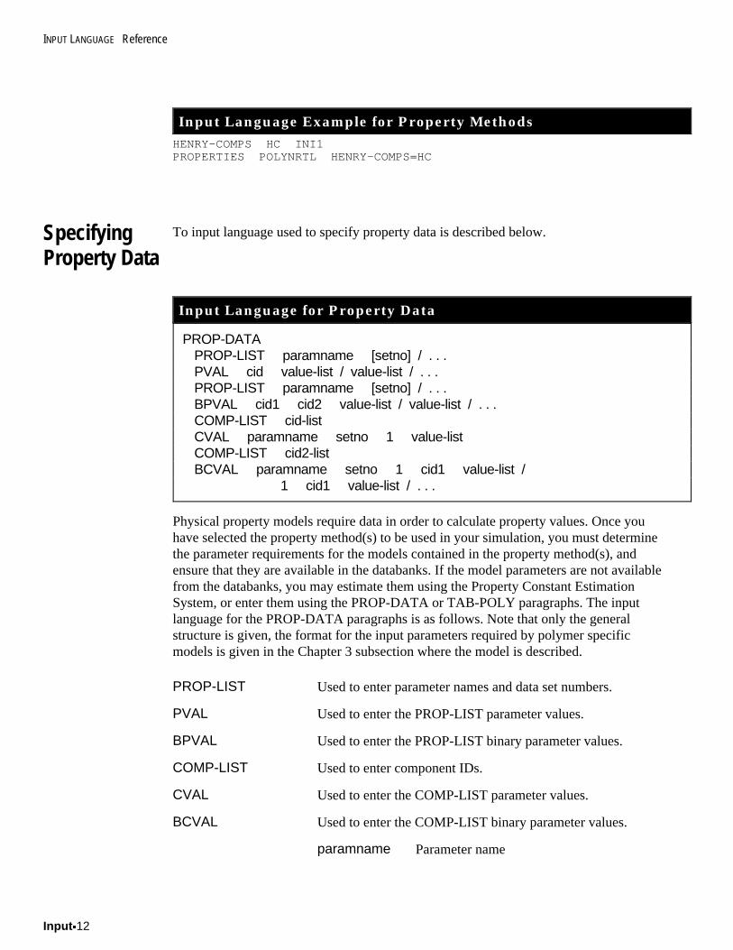
INPUT LANGUAGE Reference
Input x12
Input Language Example for Property MethodsHENRY-COMPS HC INI1PROPERTIES POLYNRTL HENRY-COMPS=HC
SpecifyingProperty Data
To input language used to specify property data is described below.
Input Language for Property Data
PROP-DATAPROP-LIST paramname [setno] / . . .PVAL cid value-list / value-list / . . .PROP-LIST paramname [setno] / . . .BPVAL cid1 cid2 value-list / value-list / . . .COMP-LIST cid-listCVAL paramname setno 1 value-listCOMP-LIST cid2-listBCVAL paramname setno 1 cid1 value-list /
1 cid1 value-list / . . .
Physical property models require data in order to calculate property values. Once youhave selected the property method(s) to be used in your simulation, you must determinethe parameter requirements for the models contained in the property method(s), andensure that they are available in the databanks. If the model parameters are not availablefrom the databanks, you may estimate them using the Property Constant EstimationSystem, or enter them using the PROP-DATA or TAB-POLY paragraphs. The inputlanguage for the PROP-DATA paragraphs is as follows. Note that only the generalstructure is given, the format for the input parameters required by polymer specificmodels is given in the Chapter 3 subsection where the model is described.
PROP-LIST Used to enter parameter names and data set numbers.
PVAL Used to enter the PROP-LIST parameter values.
BPVAL Used to enter the PROP-LIST binary parameter values.
COMP-LIST Used to enter component IDs.
CVAL Used to enter the COMP-LIST parameter values.
BCVAL Used to enter the COMP-LIST binary parameter values.
paramname Parameter name
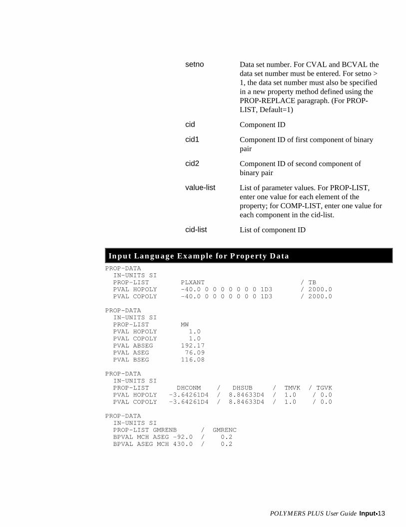
POLYMERS PLUS User Guide Input x13
setno Data set number. For CVAL and BCVAL thedata set number must be entered. For setno >1, the data set number must also be specifiedin a new property method defined using thePROP-REPLACE paragraph. (For PROP-LIST, Default=1)
cid Component ID
cid1 Component ID of first component of binarypair
cid2 Component ID of second component ofbinary pair
value-list List of parameter values. For PROP-LIST,enter one value for each element of theproperty; for COMP-LIST, enter one value foreach component in the cid-list.
cid-list List of component ID
Input Language Example for Property DataPROP-DATA IN-UNITS SI PROP-LIST PLXANT / TB PVAL HOPOLY -40.0 0 0 0 0 0 0 0 1D3 / 2000.0 PVAL COPOLY -40.0 0 0 0 0 0 0 0 1D3 / 2000.0
PROP-DATA IN-UNITS SI PROP-LIST MW PVAL HOPOLY 1.0 PVAL COPOLY 1.0 PVAL ABSEG 192.17 PVAL ASEG 76.09 PVAL BSEG 116.08
PROP-DATA IN-UNITS SI PROP-LIST DHCONM / DHSUB / TMVK / TGVK PVAL HOPOLY -3.64261D4 / 8.84633D4 / 1.0 / 0.0 PVAL COPOLY -3.64261D4 / 8.84633D4 / 1.0 / 0.0
PROP-DATA IN-UNITS SI PROP-LIST GMRENB / GMRENC BPVAL MCH ASEG -92.0 / 0.2 BPVAL ASEG MCH 430.0 / 0.2
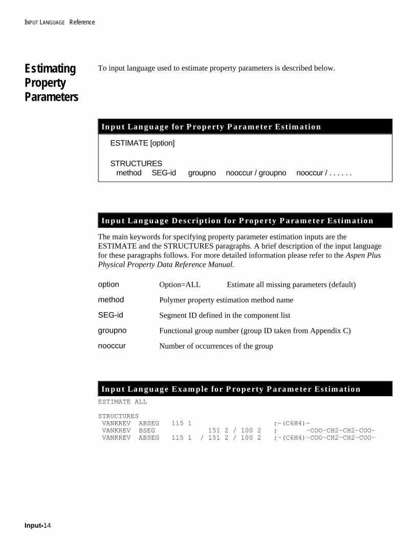
INPUT LANGUAGE Reference
Input x14
EstimatingPropertyParameters
To input language used to estimate property parameters is described below.
Input Language for Property Parameter Estimation
ESTIMATE [option]
STRUCTURES method SEG-id groupno nooccur / groupno nooccur / . . . . . .
Input Language Description for Property Parameter Estimation
The main keywords for specifying property parameter estimation inputs are theESTIMATE and the STRUCTURES paragraphs. A brief description of the input languagefor these paragraphs follows. For more detailed information please refer to the Aspen PlusPhysical Property Data Reference Manual.
option Option=ALL Estimate all missing parameters (default)
method Polymer property estimation method name
SEG-id Segment ID defined in the component list
groupno Functional group number (group ID taken from Appendix C)
nooccur Number of occurrences of the group
Input Language Example for Property Parameter EstimationESTIMATE ALL
STRUCTURES VANKREV ABSEG 115 1 ;-(C6H4)- VANKREV BSEG 151 2 / 100 2 ; -COO-CH2-CH2-COO- VANKREV ABSEG 115 1 / 151 2 / 100 2 ;-(C6H4)-COO-CH2-CH2-COO-
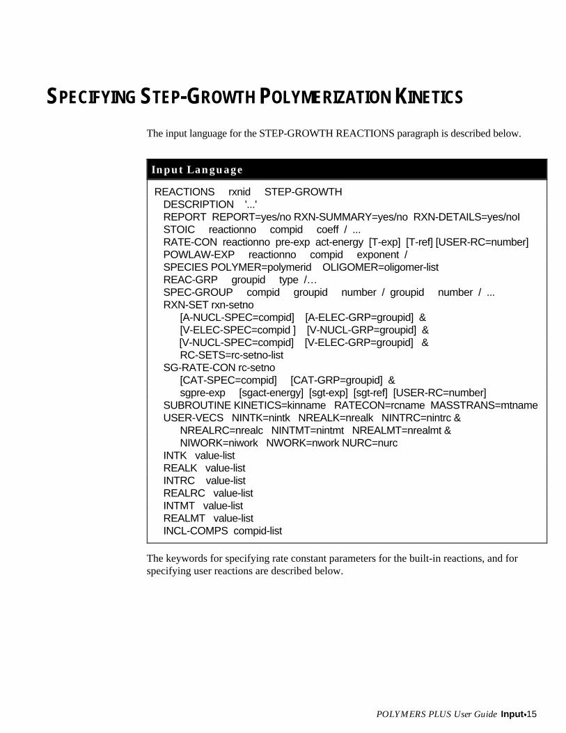
POLYMERS PLUS User Guide Input x15
SPECIFYING STEP-GROWTH POLYMERIZATION KINETICS
The input language for the STEP-GROWTH REACTIONS paragraph is described below.
Input Language
REACTIONS rxnid STEP-GROWTHDESCRIPTION '...'REPORT REPORT=yes/no RXN-SUMMARY=yes/no RXN-DETAILS=yes/noISTOIC reactionno compid coeff / ...RATE-CON reactionno pre-exp act-energy [T-exp] [T-ref] [USER-RC=number]POWLAW-EXP reactionno compid exponent /SPECIES POLYMER=polymerid OLIGOMER=oligomer-listREAC-GRP groupid type /…SPEC-GROUP compid groupid number / groupid number / ...RXN-SET rxn-setno
[A-NUCL-SPEC=compid] [A-ELEC-GRP=groupid] &[V-ELEC-SPEC=compid ] [V-NUCL-GRP=groupid] &
[V-NUCL-SPEC=compid] [V-ELEC-GRP=groupid] &RC-SETS=rc-setno-list
SG-RATE-CON rc-setno[CAT-SPEC=compid] [CAT-GRP=groupid] &sgpre-exp [sgact-energy] [sgt-exp] [sgt-ref] [USER-RC=number]
SUBROUTINE KINETICS=kinname RATECON=rcname MASSTRANS=mtnameUSER-VECS NINTK=nintk NREALK=nrealk NINTRC=nintrc &
NREALRC=nrealc NINTMT=nintmt NREALMT=nrealmt &NIWORK=niwork NWORK=nwork NURC=nurc
INTK value-listREALK value-listINTRC value-listREALRC value-listINTMT value-listREALMT value-listINCL-COMPS compid-list
The keywords for specifying rate constant parameters for the built-in reactions, and forspecifying user reactions are described below.
INPUT LANGUAGE Reference
Input x16
Input Language Description
rxnid Unique paragraph ID.
DESCRIPTION Up to 64 characters between double quotes.
REPORT Reaction report options- controls writing of reaction report in .REPfile.
REPORT=YES Print reaction report
REPORT=NO Do not print reaction report
RXN-SUMMARY=YES
Print stoichiometry for each model-generatedand user-specified reaction. (Default).
RXN-SUMMARY=NO
Do not print this summary.
RXN-DETAILS=YES Print stoichiometry, rate constants, andprobability factors for each model-generatedand user-specified reaction.
RXN-DETAILS=NO Do not print this detailed summary.
STOIC Used to specify stoichiometry for user reactions.
Reactionno Reaction number
compid Component ID
coeff Stoichiometric coefficient (positive forproducts, negative for reactants)
RATE-CON Used to specify rate constants for user reactions.
Reactionno Reaction number
pre-exp Pre-exponential factor in inverse-time units
act-energy Activation energy in mole enthalpy units
T-exp Temperature exponent
T-ref Reference temperature
number User rate constant flag
POWLAW-EXP Used to specify power-law exponents for user reactions.
reactionno Reaction number
compid Component ID
POLYMERS PLUS User Guide Input x17
exponent Power law exponent
SPECIES Used to specify key components involved in the reactions.
polymerid Component ID for polymer product
oligomer-list List of oligomers to be tracked
REAC-GRP Used to identify the names and types of reacting functional groupsparticipating in the reaction network.
groupid Functional group ID
type Functional group type
EE-GRP Electrophilic repeat unit
NN-GRP Nucleophilic repeat unit
EN-GRP Mixed electrophilic/nucleophilic repeat unit
E-GRP Electrophilic leaving group
N-GRP Nucleophilic leaving group
EX-GRP Electrophilic modifier (end cap)
NX-GRP Nucleophilic modifier (end cap)
SPEC-GROUP Used to characterize the reacting functional group composition of thecomponents (segments and monomers) participating in the step-growth reaction network.
compid Component ID
groupid Reactive functional group ID
number Number of occurrences of group in species
SG-RATE-CON Used to specify rate constants for model-generated step-growthreactions and to specify which catalyst they apply to (if any).
setno Rate constant set number
CAT-SPEC=compid Component ID of catalyst species
CAT-GRP=groupid Group ID of catalyst group
USER-RC=number User rate expression flag
sgpre-exp Pre-exponential factor in inverse-time units
sgact-energy Activation energy in mole-enthalpy units
INPUT LANGUAGE Reference
Input x18
sgt-exp Temperature exponent
sgt-ref Reference temperature in temperature units
RXN-SET Used to assign sets of rate constants to model-generated reactions.
A-NUCL-SPEC=compid
Component ID of reactant which acts as theattacking nucleophile
A-ELEC-GRP=groupid
Group ID of electrophilic leaving group inattacking nucleophilic reactant
V-ELEC-SPEC=compid
Component ID of reactant which acts as thenucleophile. When reactions occur insidepolymer molecules, this may be a segment.
V-ELEC-GRP=groupid
Group ID of electrophilic group in victimspecies (attached to V-NUCL-GRP)
V-NUCL-SPEC=compid
Component ID of nucleophilic reactantattached to the victim electrophilic reactantat the reacting site
V-NUCL-GRP=groupid
Group ID of nucleophilic group in victimspecies (attached to V-ELEC-GRP)
RC-SETS =rcsetno-list
List of rate constants (from SG-RATE-CON)which apply to the set of reactions identifiedby the previous keywords
SUBROUTINE Used to provide the names of user-supplied Fortran subroutines. Thesubroutine argument lists are documented in Tables 4.38-4.40.
KINETICS=kinname User kinetic subroutine name
RATECON=rcname User rate constant subroutine name
MASSTRAN=mtname
User concentration basis / mass-transfersubroutine name
USER-VECS Used to specify the size of vectors for user subroutines.
NINTK=nintk Length of integer array for kinetics
NREALK=nrealk Length of real array for kinetics
NINTRC=nintrc Length of integer array for rate constants
NREALRC=nrealrc Length of real array for rate constants
NINTMT=nintmt Length of integer array for mass transfer
POLYMERS PLUS User Guide Input x19
NREALMT=nrealmt Length of real array for mass transfer
NIWORK=niwork Total length of integer workspace
NWORK=nwork Total length of real workspace
INTK Used to enter integer parameter for kinetics.
REALK Used to enter real parameters for kinetics.
INTRC Used to enter integer parameters for rate constants.
REALRC Used to enter real parameters for rate constants.
INTMT Used to enter integer parameters for mass transfer.
REALMT Used to enter real parameters for mass transfer.
INCL-COMPS Used to list components which participate in reactions in the userkinetics model, but which do not appear in model-generated or user-specified reactions.
Compid-list List of additional components to include inthe mass-balance calculations
Input Language ExampleREACTIONS NYLON STEP-GROWTH DESCRIPTION “NYLON-6 KINETICS: SIMPLE MODEL WITHOUT CYCLICS” REPORT RXN-DETAILS=YES SPECIES POLYMER=NYLON6 REAC-GROUP TNH2 E-GRP / TCOOH N-GRP / BCAP EN-GRP SPECIES-GRP T-NH2 TNH2 1 / T-NH2 BCAP 1 / T-COOH TCOOH 1 / & T-COOH BCAP 1 / ACA TNH2 1 / ACA TCOOH 1 / & ACA BCAP 1 / B-ACA BCAP 1 / H2O TNH2 1 / H2O TCOOH 1 SG-RATE-CON 1 TREF=260 PRE-EXP= 5.461 ACT-ENERGY=23.271 SG-RATE-CON 2 CAT-SPEC=ACA TREF=260 PRE-EXP=40.678 ACT-ENERGY=20.670 SG-RATE-CON 3 CAT-SPEC=T-COOH TREF=260 PRE-EXP=40.678 ACT-ENERGY=20.670 SG-RATE-CON 4 TREF=260 PRE-EXP=0.0124 ACT-ENERGY=29.217 SG-RATE-CON 5 CAT-SPEC=ACA TREF=260 PRE-EXP=0.0924 ACT-ENERGY=26.616 SG-RATE-CON 6 CAT-SPEC=T-COOH TREF=260 PRE-EXP=0.0924 ACT-ENERGY=26.616 RXN-SET 1 ELECTRO-GRP=TNH2 NUCLEO-GRP=TCOOH RC-SETS= 1 2 3 RXN-SET 2 NUCLEOPHILE=H2O RC-SETS= 4 5 6
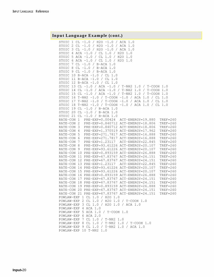
INPUT LANGUAGE Reference
Input x20
Input Language Example (cont.) STOIC 1 CL -1.0 / H2O -1.0 / ACA 1.0 STOIC 2 CL -1.0 / H2O -1.0 / ACA 1.0 STOIC 3 CL -1.0 / H2O -1.0 / ACA 1.0 STOIC 4 ACA -1.0 / CL 1.0 / H2O 1.0 STOIC 5 ACA -1.0 / CL 1.0 / H2O 1.0 STOIC 6 ACA -1.0 / CL 1.0 / H2O 1.0 STOIC 7 CL -1.0 / B-ACA 1.0 STOIC 8 CL -1.0 / B-ACA 1.0 STOIC 9 CL -1.0 / B-ACA 1.0 STOIC 10 B-ACA -1.0 / CL 1.0 STOIC 11 B-ACA -1.0 / CL 1.0 STOIC 12 B-ACA -1.0 / CL 1.0 STOIC 13 CL -1.0 / ACA -1.0 / T-NH2 1.0 / T-COOH 1.0 STOIC 14 CL -1.0 / ACA -1.0 / T-NH2 1.0 / T-COOH 1.0 STOIC 15 CL -1.0 / ACA -1.0 / T-NH2 1.0 / T-COOH 1.0 STOIC 16 T-NH2 -1.0 / T-COOH -1.0 / ACA 1.0 / CL 1.0 STOIC 17 T-NH2 -1.0 / T-COOH -1.0 / ACA 1.0 / CL 1.0 STOIC 18 T-NH2 -1.0 / T-COOH -1.0 / ACA 1.0 / CL 1.0 STOIC 19 CL -1.0 / B-ACA 1.0 STOIC 20 CL -1.0 / B-ACA 1.0 STOIC 21 CL -1.0 / B-ACA 1.0 RATE-CON 1 PRE-EXP=0.00424 ACT-ENERGY=19.880 TREF=260 RATE-CON 2 PRE-EXP=0.840712 ACT-ENERGY=18.806 TREF=260 RATE-CON 3 PRE-EXP=0.840712 ACT-ENERGY=18.806 TREF=260 RATE-CON 4 PRE-EXP=1.370519 ACT-ENERGY=17.962 TREF=260 RATE-CON 5 PRE-EXP=271.7817 ACT-ENERGY=16.888 TREF=260 RATE-CON 6 PRE-EXP=271.7817 ACT-ENERGY=16.888 TREF=260 RATE-CON 7 PRE-EXP=1.23117 ACT-ENERGY=22.845 TREF=260 RATE-CON 8 PRE-EXP=93.61226 ACT-ENERGY=20.107 TREF=260 RATE-CON 9 PRE-EXP=93.61226 ACT-ENERGY=20.107 TREF=260 RATE-CON 10 PRE-EXP=0.893159 ACT-ENERGY=26.888 TREF=260 RATE-CON 11 PRE-EXP=67.83767 ACT-ENERGY=24.151 TREF=260 RATE-CON 12 PRE-EXP=67.83767 ACT-ENERGY=24.151 TREF=260 RATE-CON 13 PRE-EXP=1.23117 ACT-ENERGY=22.845 TREF=260 RATE-CON 14 PRE-EXP=93.61226 ACT-ENERGY=20.107 TREF=260 RATE-CON 15 PRE-EXP=93.61226 ACT-ENERGY=20.107 TREF=260 RATE-CON 16 PRE-EXP=0.893159 ACT-ENERGY=26.888 TREF=260 RATE-CON 17 PRE-EXP=67.83767 ACT-ENERGY=24.151 TREF=260 RATE-CON 18 PRE-EXP=67.83767 ACT-ENERGY=24.151 TREF=260 RATE-CON 19 PRE-EXP=0.893159 ACT-ENERGY=26.888 TREF=260 RATE-CON 20 PRE-EXP=67.83767 ACT-ENERGY=24.151 TREF=260 RATE-CON 21 PRE-EXP=67.83767 ACT-ENERGY=24.151 TREF=260 POWLAW-EXP 1 CL 1.0 / H2O 1.0 POWLAW-EXP 2 CL 1.0 / H2O 1.0 / T-COOH 1.0 POWLAW-EXP 3 CL 1.0 / H2O 1.0 / ACA 1.0 POWLAW-EXP 4 ACA 1.0 POWLAW-EXP 5 ACA 1.0 / T-COOH 1.0 POWLAW-EXP 6 ACA 2.0 POWLAW-EXP 7 CL 1.0 / T-NH2 1.0 POWLAW-EXP 8 CL 1.0 / T-NH2 1.0 / T-COOH 1.0 POWLAW-EXP 9 CL 1.0 / T-NH2 1.0 / ACA 1.0 POWLAW-EXP 10 T-NH2 1.0
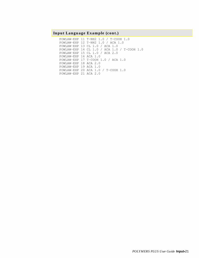
POLYMERS PLUS User Guide Input x21
Input Language Example (cont.) POWLAW-EXP 11 T-NH2 1.0 / T-COOH 1.0 POWLAW-EXP 12 T-NH2 1.0 / ACA 1.0 POWLAW-EXP 13 CL 1.0 / ACA 1.0 POWLAW-EXP 14 CL 1.0 / ACA 1.0 / T-COOH 1.0 POWLAW-EXP 15 CL 1.0 / ACA 2.0 POWLAW-EXP 16 ACA 1.0 POWLAW-EXP 17 T-COOH 1.0 / ACA 1.0 POWLAW-EXP 18 ACA 2.0 POWLAW-EXP 19 ACA 1.0 POWLAW-EXP 20 ACA 1.0 / T-COOH 1.0 POWLAW-EXP 21 ACA 2.0
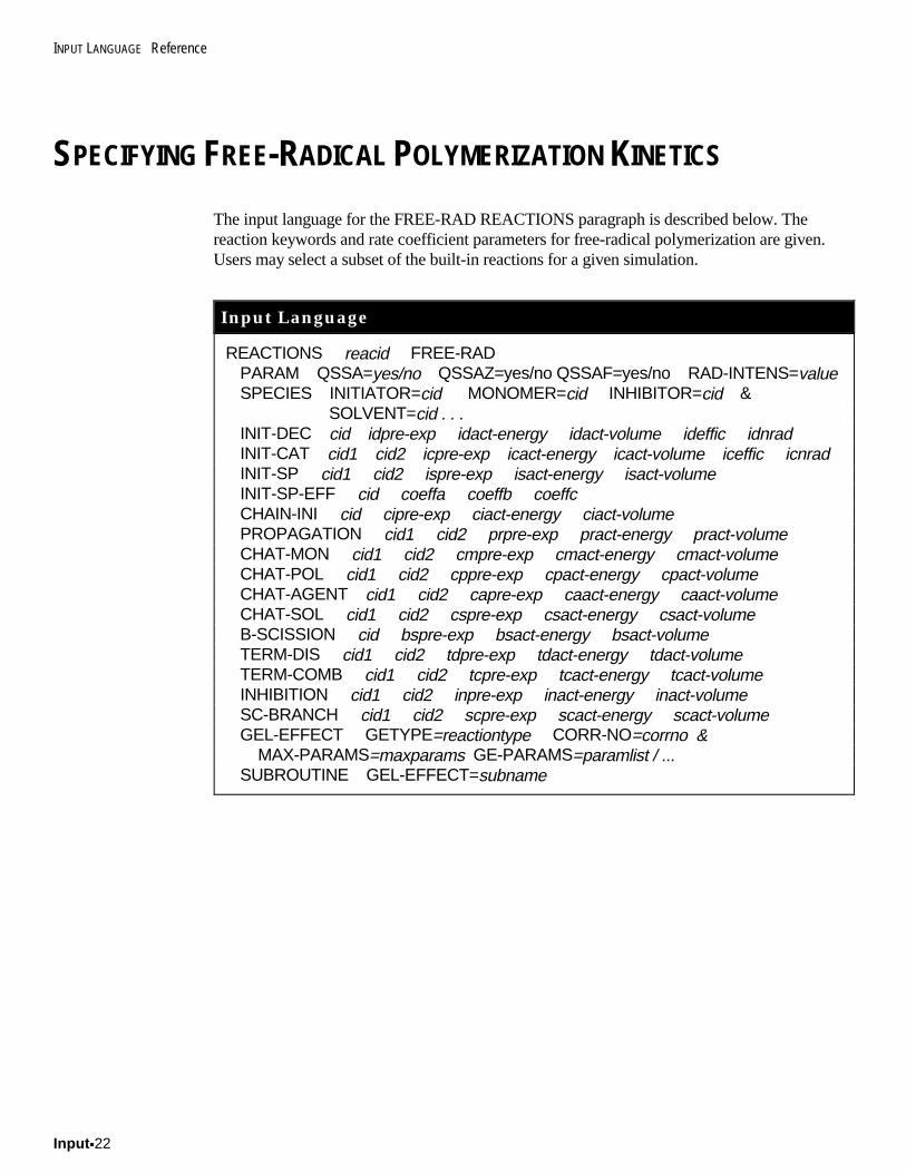
INPUT LANGUAGE Reference
Input x22
SPECIFYING FREE-RADICAL POLYMERIZATION KINETICS
The input language for the FREE-RAD REACTIONS paragraph is described below. Thereaction keywords and rate coefficient parameters for free-radical polymerization are given.Users may select a subset of the built-in reactions for a given simulation.
Input Language
REACTIONS reacid FREE-RADPARAM QSSA=yes/no QSSAZ=yes/no QSSAF=yes/no RAD-INTENS=valueSPECIES INITIATOR=cid MONOMER=cid INHIBITOR=cid &
SOLVENT=cid . . .INIT-DEC cid idpre-exp idact-energy idact-volume ideffic idnradINIT-CAT cid1 cid2 icpre-exp icact-energy icact-volume iceffic icnradINIT-SP cid1 cid2 ispre-exp isact-energy isact-volumeINIT-SP-EFF cid coeffa coeffb coeffcCHAIN-INI cid cipre-exp ciact-energy ciact-volumePROPAGATION cid1 cid2 prpre-exp pract-energy pract-volumeCHAT-MON cid1 cid2 cmpre-exp cmact-energy cmact-volumeCHAT-POL cid1 cid2 cppre-exp cpact-energy cpact-volumeCHAT-AGENT cid1 cid2 capre-exp caact-energy caact-volumeCHAT-SOL cid1 cid2 cspre-exp csact-energy csact-volumeB-SCISSION cid bspre-exp bsact-energy bsact-volumeTERM-DIS cid1 cid2 tdpre-exp tdact-energy tdact-volumeTERM-COMB cid1 cid2 tcpre-exp tcact-energy tcact-volumeINHIBITION cid1 cid2 inpre-exp inact-energy inact-volumeSC-BRANCH cid1 cid2 scpre-exp scact-energy scact-volumeGEL-EFFECT GETYPE=reactiontype CORR-NO=corrno & MAX-PARAMS=maxparams GE-PARAMS=paramlist / ...SUBROUTINE GEL-EFFECT=subname
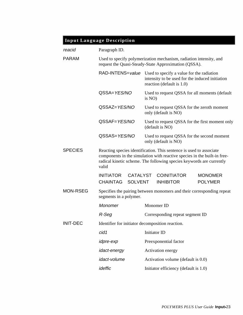
POLYMERS PLUS User Guide Input x23
Input Language Description
reacid Paragraph ID.
PARAM Used to specify polymerization mechanism, radiation intensity, andrequest the Quasi-Steady-State Approximation (QSSA).
RAD-INTENS=value Used to specify a value for the radiationintensity to be used for the induced initiationreaction (default is 1.0)
QSSA=YES/NO Used to request QSSA for all moments (defaultis NO)
QSSAZ=YES/NO Used to request QSSA for the zeroth momentonly (default is NO)
QSSAF=YES/NO Used to request QSSA for the first moment only(default is NO)
QSSAS=YES/NO Used to request QSSA for the second momentonly (default is NO)
SPECIES Reacting species identification. This sentence is used to associatecomponents in the simulation with reactive species in the built-in free-radical kinetic scheme. The following species keywords are currentlyvalid
INITIATOR CATALYST COINITIATOR MONOMERCHAINTAG SOLVENT INHIBITOR POLYMER
MON-RSEG Specifies the pairing between monomers and their corresponding repeatsegments in a polymer.
Monomer Monomer ID
R-Seg Corresponding repeat segment ID
INIT-DEC Identifier for initiator decomposition reaction.
cid1 Initiator ID
idpre-exp Preexponential factor
idact-energy Activation energy
idact-volume Activation volume (default is 0.0)
ideffic Initiator efficiency (default is 1.0)
INPUT LANGUAGE Reference
Input x24
idnrad Number of radicals from one initiator molecule(default is 2.0)
INIT-CAT Identifier for catalyzed initiator decomposition reaction.
cid1 Initiator ID
cid2 Catalyst ID
icpre-exp Preexponential factor
icact-energy Activation energy
icact-volume Activation volume (default is 0.0)
iceffic Initiator efficiency (default is 1.0)
icnrad Number of radicals from one initiator molecule(default is 2.0)
INIT-SP Identifier for thermal and radiation induced initiation reaction.
cid1 Monomer ID
cid2 Co-initiator ID
ispre-exp Preexponential factor
isact-energy Activation energy
isact-volume Activation volume (default is 0.0)
INIT-SP-EFF Parameters for thermal and radiation induced initiation reaction.
cid Monomer ID
coeffa Exponent for coinitiator concentration (defaultis 0.0)
coeffb Exponent for monomer concentration (default is0.0)
coeffc Exponent for radiation intensity (default is 0.0)
CHAIN-INI Identifier for chain initiation reaction.
cid1 Monomer ID
cipre-exp Preexponential factor
ciact-energy Activation energy
ciact-volume Activation volume (default is 0.0)
POLYMERS PLUS User Guide Input x25
PROPAGATION Identifier for chain propagation reaction.
cid1 Monomer corresponding to polymer activesegment ID
cid2 Monomer ID
prpre-exp Preexponential factor
pract-energy Activation energy
pract-volume Activation volume (default is 0.0)
CHAT-MON Identifier for chain transfer to monomer reaction.
cid1 Monomer corresponding to polymer activesegment ID
cid2 Monomer ID
cmpre-exp Preexponential factor
cmact-energy Activation energy
cmact-volume Activation volume (default is 0.0)
CHAT-POL Identifier for chain transfer to polymer reaction.
cid1 Monomer corresponding to polymer activesegment ID
cid2 Monomer corresponding to polymer reactingsegment ID on dead chain
cppre-exp Preexponential factor
cpact-energy Activation energy
cpact-volume Activation volume (default is 0.0)
CHAT-AGENT Identifier for chain transfer to transfer agent reaction.
cid1 Monomer corresponding to polymer activesegment ID
cid2 Transfer agent ID
capre-exp Preexponential factor
caact-energy Activation energy
caact-volume Activation volume (default is 0.0)
INPUT LANGUAGE Reference
Input x26
CHAT-SOL Identifier for chain transfer to solvent reaction.
cid1 Monomer corresponding it polymer activesegment ID
cid2 Solvent ID
cspre-exp Preexponential factor
csact-energy Activation energy
csact-volume Activation volume (default is 0.0)
B-SCISSION Identifier for beta-scission reaction.
cid1 Monomer corresponding to polymer activesegment ID
bspre-exp Preexponential factor
bsact-energy Activation energy
bsact-volume Activation volume (default is 0.0)
TERM-DIS Identifier for chain termination by disproportionation reaction.
cid1 Monomer corresponding to first polymer activesegment ID
cid2 Monomer corresponding to second polymeractive segment ID
tdpre-exp Preexponential factor
tdact-energy Activation energy
tdact-volume Activation volume (default is 0.0)
TERM-COMB Identifier for chain termination by combination reaction.
cid1 Monomer corresponding to first polymer activesegment ID
cid2 Monomer corresponding to second polymeractive segment ID
tcpre-exp Preexponential factor
tcact-energy Activation energy
tcact-volume Activation volume (default is 0.0)
POLYMERS PLUS User Guide Input x27
INHIBITION Identifier for chain inhibition reaction.
cid1 Monomer corresponding to polymer activesegment ID
cid2 Inhibitor ID
inpre-exp Preexponential factor
inact-energy Activation energy
inact-volume Activation volume (default is 0.0)
SC-BRANCH Identifier for short chain branching reaction.
cid1 Monomer corresponding to reactant polymeractive segment ID
cid2 Monomer corresponding to product activesegment ID
scpre-exp Preexponential factor
scact-energy Activation energy
scact-volume Activation volume (default is 0.0)
GEL-EFFECT Gel effect switch and correlation selection. This sentence is used to
�� Include a gel effect for any reactions in the built-in kinetic schemeand for the initiator efficiency
�� Select a gel effect correlation from a list of built-in and user specifiedgel effect correlations
�� Specify the maximum number of parameters
�� Specify the parameter values for the selected correlation
The default action is to not include a gel effect.
GETYPE=reactiontype
Used to identify the type of reaction to apply geleffect to. A list of valid reaction types follows
INITIATION Initiator decomposition
INIT-EFF Initiator efficiency
PROPAGATION Propagation, chain initiation and inducedinitiation reactions
CHAT-MON Chain transfer to monomer
INPUT LANGUAGE Reference
Input x28
CHAT-POL Chain transfer to polymer
CHAT-AGENT Chain transfer to agent
CHAT-SOL Chain transfer to solvent
TERMINATION Termination
CORR-NO=corrno Used to select a correlation number. If acorrelation number greater than the number ofbuilt-in correlations (currently 2) is specifiedthen the user should supply a Fortran subroutinecontaining the user gel effect correlation.
MAX-PARAMS=maxparams
Used to enter the maximum number of gel effectparameters for the correlation selected.
GE-PARAMS=paramlist
Used to enter a list of parameters for thecorrelation selected.
SUBROUTINE User subroutines sentence.
GEL-EFFECT=subname
Used to specify the name of the subroutinecontaining user gel effect correlations. The usergel-effect subroutine argument list was shown inTable 4.42. A Fortran template calledUSRGEL.F is available for your use.
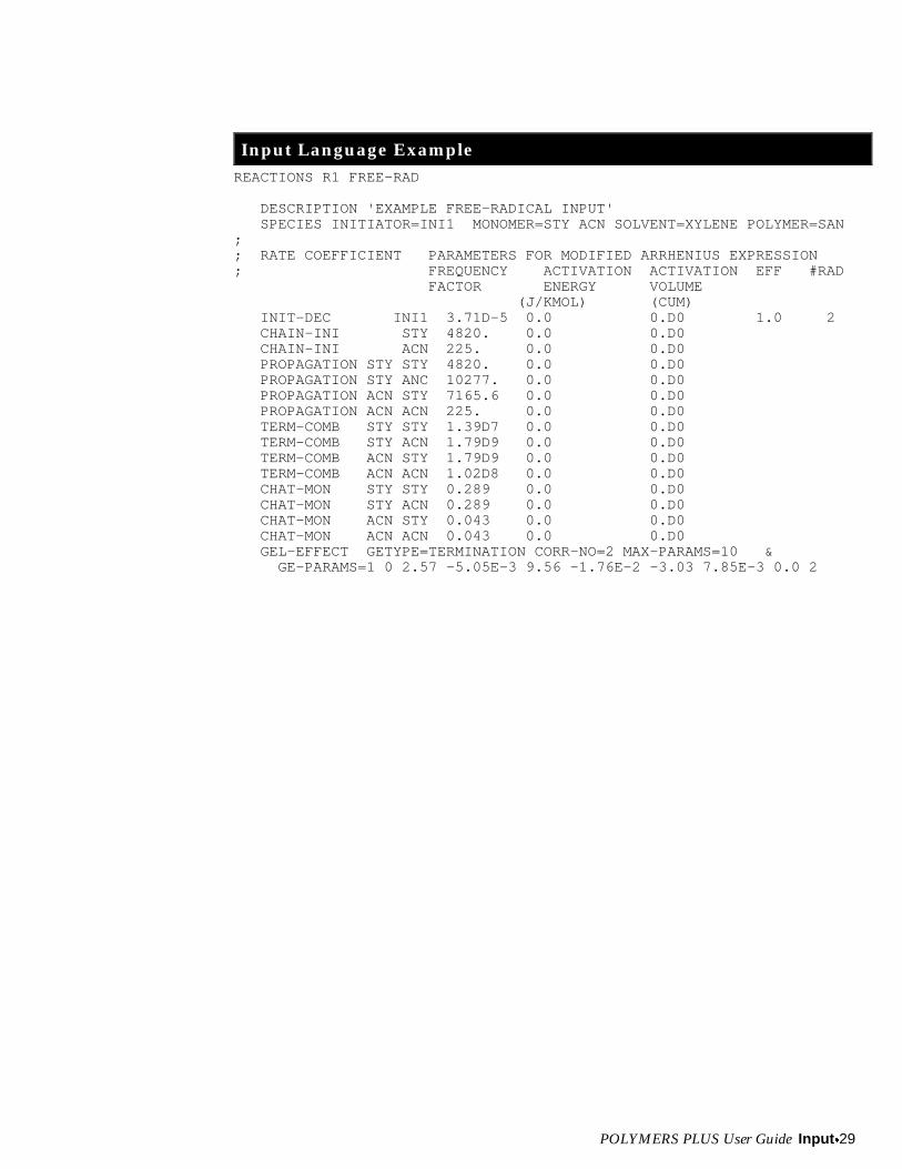
POLYMERS PLUS User Guide Input x29
Input Language ExampleREACTIONS R1 FREE-RAD
DESCRIPTION 'EXAMPLE FREE-RADICAL INPUT' SPECIES INITIATOR=INI1 MONOMER=STY ACN SOLVENT=XYLENE POLYMER=SAN;; RATE COEFFICIENT PARAMETERS FOR MODIFIED ARRHENIUS EXPRESSION; FREQUENCY ACTIVATION ACTIVATION EFF #RAD FACTOR ENERGY VOLUME (J/KMOL) (CUM) INIT-DEC INI1 3.71D-5 0.0 0.D0 1.0 2 CHAIN-INI STY 4820. 0.0 0.D0 CHAIN-INI ACN 225. 0.0 0.D0 PROPAGATION STY STY 4820. 0.0 0.D0 PROPAGATION STY ANC 10277. 0.0 0.D0 PROPAGATION ACN STY 7165.6 0.0 0.D0 PROPAGATION ACN ACN 225. 0.0 0.D0 TERM-COMB STY STY 1.39D7 0.0 0.D0 TERM-COMB STY ACN 1.79D9 0.0 0.D0 TERM-COMB ACN STY 1.79D9 0.0 0.D0 TERM-COMB ACN ACN 1.02D8 0.0 0.D0 CHAT-MON STY STY 0.289 0.0 0.D0 CHAT-MON STY ACN 0.289 0.0 0.D0 CHAT-MON ACN STY 0.043 0.0 0.D0 CHAT-MON ACN ACN 0.043 0.0 0.D0 GEL-EFFECT GETYPE=TERMINATION CORR-NO=2 MAX-PARAMS=10 & GE-PARAMS=1 0 2.57 -5.05E-3 9.56 -1.76E-2 -3.03 7.85E-3 0.0 2
INPUT LANGUAGE Reference
Input x30
SPECIFYING EMULSION POLYMERIZATION KINETICS
The input language for the EMULSION REACTIONS paragraph is described below. Usersare able to select the phases in which the reactions are occurring and also define the kineticsof particle absorption, desorption, and termination.
Input Language
REACTIONS reacid EMULSIONPARAM KBASIS=mole/massSPLIT-PM spm-cid kllSPECIES INITIATOR=cid MONOMER=cid INHIBITOR=cid &
DISPERSANT=cid . . .INIT-DEC phasid cid idpre-exp idact-energy [idact-volume] ideffic idnradINIT-CAT phasid cid1 cid2 icpre-exp icact-energy [icact-volume] iceffic icnradINIT-SP phasid cid1 cid2 ispre-exp isact-energy [isact-volume]INIT-ACT phasid cid1 cid2 iapre-exp iaact-energy [iaact-volume] iaeffic ianradCHAIN-INI phasid cid cipre-exp ciact-energy [ciact-volume]PROPAGATION phasid cid1 cid2 prpre-exp pract-energy [pract-volume]CHAT-MON phasid cid1 cid2 cmpre-exp cmact-energy [cmact-volume]CHAT-POL phasid cid1 cid2 cppre-exp cpact-energy [cpact-volume]CHAT-AGENT phasid cid1 cid2 capre-exp caact-energy [caact-volume]B-SCISSION phasid cid bspre-exp bsact-energy [bsact-volume]TERM-DIS phasid cid1 cid2 tdpre-exp tdact-energy [tdact-volume]TERM-COMB phasid cid1 cid2 tcpre-exp tcact-energy [tcact-volume]INHIBITION phasid cid1 cid2 inpre-exp inact-energy [inact-volume]SC-BRANCH phasid cid1 cid2 scpre-exp scact-energy [scact-volume]REDUCTION phasid cid1 cid2 rdpre-exp rdact-energy [rdact-volume] rdeffic rdnradOXIDATION phasid cid1 cid2 oxpre-exp oxact-energy [oxact-volumeINIT-SP-EFF cid coeffa coeffb coeffcGEL-EFFECT GETYPE=reactiontype CORR-NO=corrno & MAX-PARAMS=maxparams GE-PARAMS=paramlist / ...SUBROUTINE GEL-EFFECT=subnameABS-MIC ampre-exp amact-energyABS-PART appre-exp apact-energyDES-PART dppre-exp dpact-energyEMUL-PARAMS emulid cmc-conc area
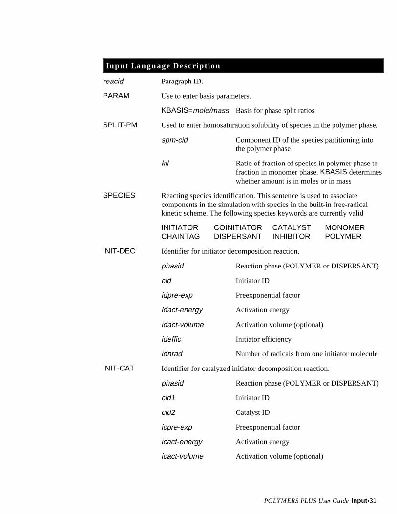
POLYMERS PLUS User Guide Input x31
Input Language Description
reacid Paragraph ID.
PARAM Use to enter basis parameters.
KBASIS=mole/mass Basis for phase split ratios
SPLIT-PM Used to enter homosaturation solubility of species in the polymer phase.
spm-cid Component ID of the species partitioning intothe polymer phase
kll Ratio of fraction of species in polymer phase tofraction in monomer phase. KBASIS determineswhether amount is in moles or in mass
SPECIES Reacting species identification. This sentence is used to associatecomponents in the simulation with species in the built-in free-radicalkinetic scheme. The following species keywords are currently valid
INITIATOR COINITIATOR CATALYST MONOMERCHAINTAG DISPERSANT INHIBITOR POLYMER
INIT-DEC Identifier for initiator decomposition reaction.
phasid Reaction phase (POLYMER or DISPERSANT)
cid Initiator ID
idpre-exp Preexponential factor
idact-energy Activation energy
idact-volume Activation volume (optional)
ideffic Initiator efficiency
idnrad Number of radicals from one initiator molecule
INIT-CAT Identifier for catalyzed initiator decomposition reaction.
phasid Reaction phase (POLYMER or DISPERSANT)
cid1 Initiator ID
cid2 Catalyst ID
icpre-exp Preexponential factor
icact-energy Activation energy
icact-volume Activation volume (optional)
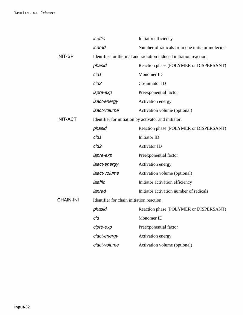
INPUT LANGUAGE Reference
Input x32
iceffic Initiator efficiency
icnrad Number of radicals from one initiator molecule
INIT-SP Identifier for thermal and radiation induced initiation reaction.
phasid Reaction phase (POLYMER or DISPERSANT)
cid1 Monomer ID
cid2 Co-initiator ID
ispre-exp Preexponential factor
isact-energy Activation energy
isact-volume Activation volume (optional)
INIT-ACT Identifier for initiation by activator and initiator.
phasid Reaction phase (POLYMER or DISPERSANT)
cid1 Initiator ID
cid2 Activator ID
iapre-exp Preexponential factor
iaact-energy Activation energy
iaact-volume Activation volume (optional)
iaeffic Initiator activation efficiency
ianrad Initiator activation number of radicals
CHAIN-INI Identifier for chain initiation reaction.
phasid Reaction phase (POLYMER or DISPERSANT)
cid Monomer ID
cipre-exp Preexponential factor
ciact-energy Activation energy
ciact-volume Activation volume (optional)
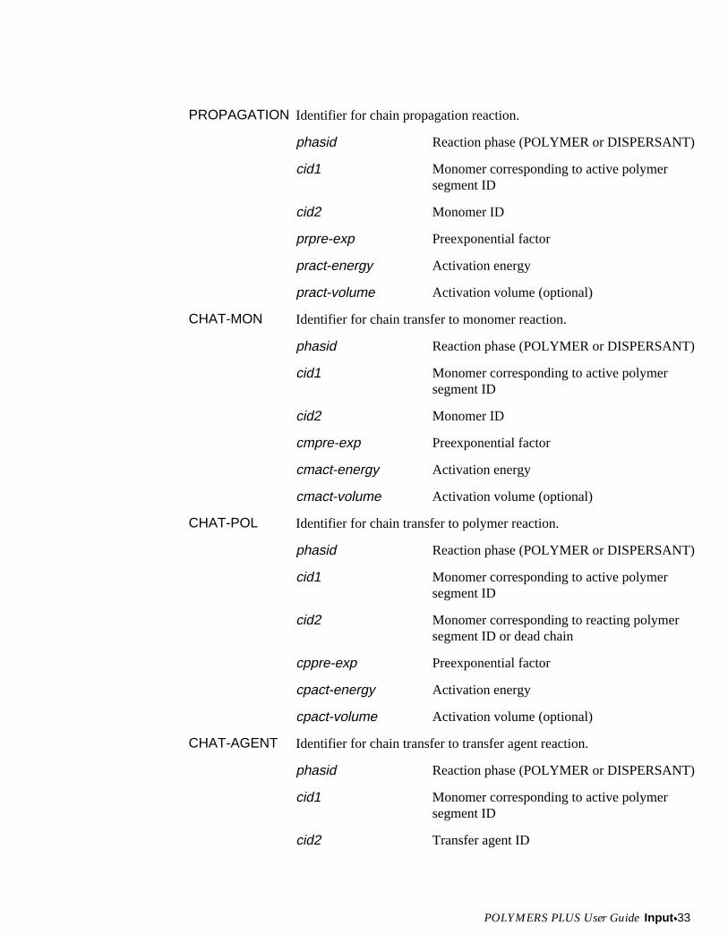
POLYMERS PLUS User Guide Input x33
PROPAGATION Identifier for chain propagation reaction.
phasid Reaction phase (POLYMER or DISPERSANT)
cid1 Monomer corresponding to active polymersegment ID
cid2 Monomer ID
prpre-exp Preexponential factor
pract-energy Activation energy
pract-volume Activation volume (optional)
CHAT-MON Identifier for chain transfer to monomer reaction.
phasid Reaction phase (POLYMER or DISPERSANT)
cid1 Monomer corresponding to active polymersegment ID
cid2 Monomer ID
cmpre-exp Preexponential factor
cmact-energy Activation energy
cmact-volume Activation volume (optional)
CHAT-POL Identifier for chain transfer to polymer reaction.
phasid Reaction phase (POLYMER or DISPERSANT)
cid1 Monomer corresponding to active polymersegment ID
cid2 Monomer corresponding to reacting polymersegment ID or dead chain
cppre-exp Preexponential factor
cpact-energy Activation energy
cpact-volume Activation volume (optional)
CHAT-AGENT Identifier for chain transfer to transfer agent reaction.
phasid Reaction phase (POLYMER or DISPERSANT)
cid1 Monomer corresponding to active polymersegment ID
cid2 Transfer agent ID
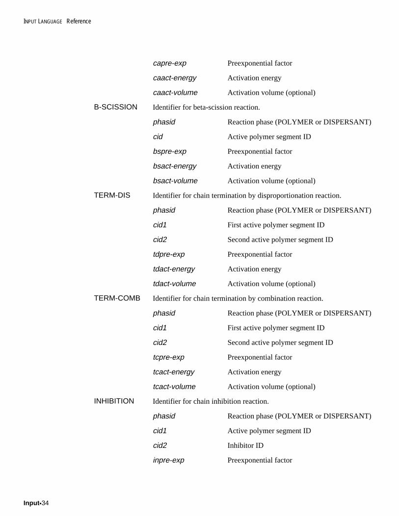
INPUT LANGUAGE Reference
Input x34
capre-exp Preexponential factor
caact-energy Activation energy
caact-volume Activation volume (optional)
B-SCISSION Identifier for beta-scission reaction.
phasid Reaction phase (POLYMER or DISPERSANT)
cid Active polymer segment ID
bspre-exp Preexponential factor
bsact-energy Activation energy
bsact-volume Activation volume (optional)
TERM-DIS Identifier for chain termination by disproportionation reaction.
phasid Reaction phase (POLYMER or DISPERSANT)
cid1 First active polymer segment ID
cid2 Second active polymer segment ID
tdpre-exp Preexponential factor
tdact-energy Activation energy
tdact-volume Activation volume (optional)
TERM-COMB Identifier for chain termination by combination reaction.
phasid Reaction phase (POLYMER or DISPERSANT)
cid1 First active polymer segment ID
cid2 Second active polymer segment ID
tcpre-exp Preexponential factor
tcact-energy Activation energy
tcact-volume Activation volume (optional)
INHIBITION Identifier for chain inhibition reaction.
phasid Reaction phase (POLYMER or DISPERSANT)
cid1 Active polymer segment ID
cid2 Inhibitor ID
inpre-exp Preexponential factor
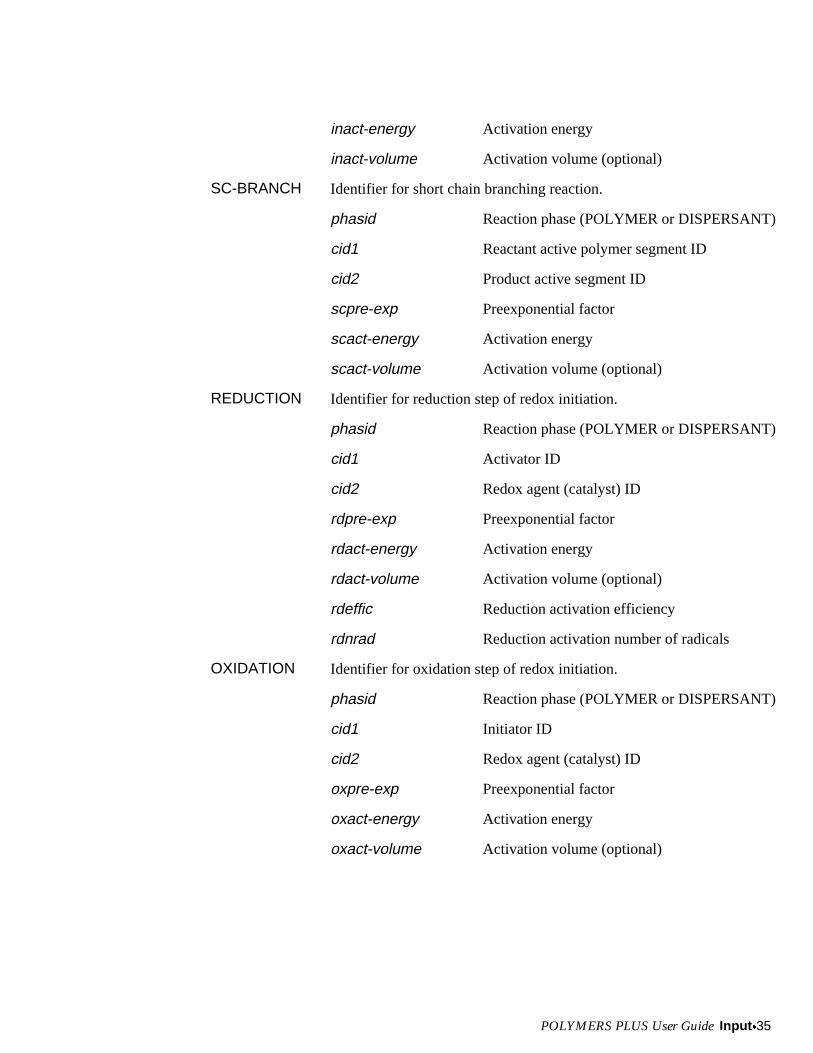
POLYMERS PLUS User Guide Input x35
inact-energy Activation energy
inact-volume Activation volume (optional)
SC-BRANCH Identifier for short chain branching reaction.
phasid Reaction phase (POLYMER or DISPERSANT)
cid1 Reactant active polymer segment ID
cid2 Product active segment ID
scpre-exp Preexponential factor
scact-energy Activation energy
scact-volume Activation volume (optional)
REDUCTION Identifier for reduction step of redox initiation.
phasid Reaction phase (POLYMER or DISPERSANT)
cid1 Activator ID
cid2 Redox agent (catalyst) ID
rdpre-exp Preexponential factor
rdact-energy Activation energy
rdact-volume Activation volume (optional)
rdeffic Reduction activation efficiency
rdnrad Reduction activation number of radicals
OXIDATION Identifier for oxidation step of redox initiation.
phasid Reaction phase (POLYMER or DISPERSANT)
cid1 Initiator ID
cid2 Redox agent (catalyst) ID
oxpre-exp Preexponential factor
oxact-energy Activation energy
oxact-volume Activation volume (optional)
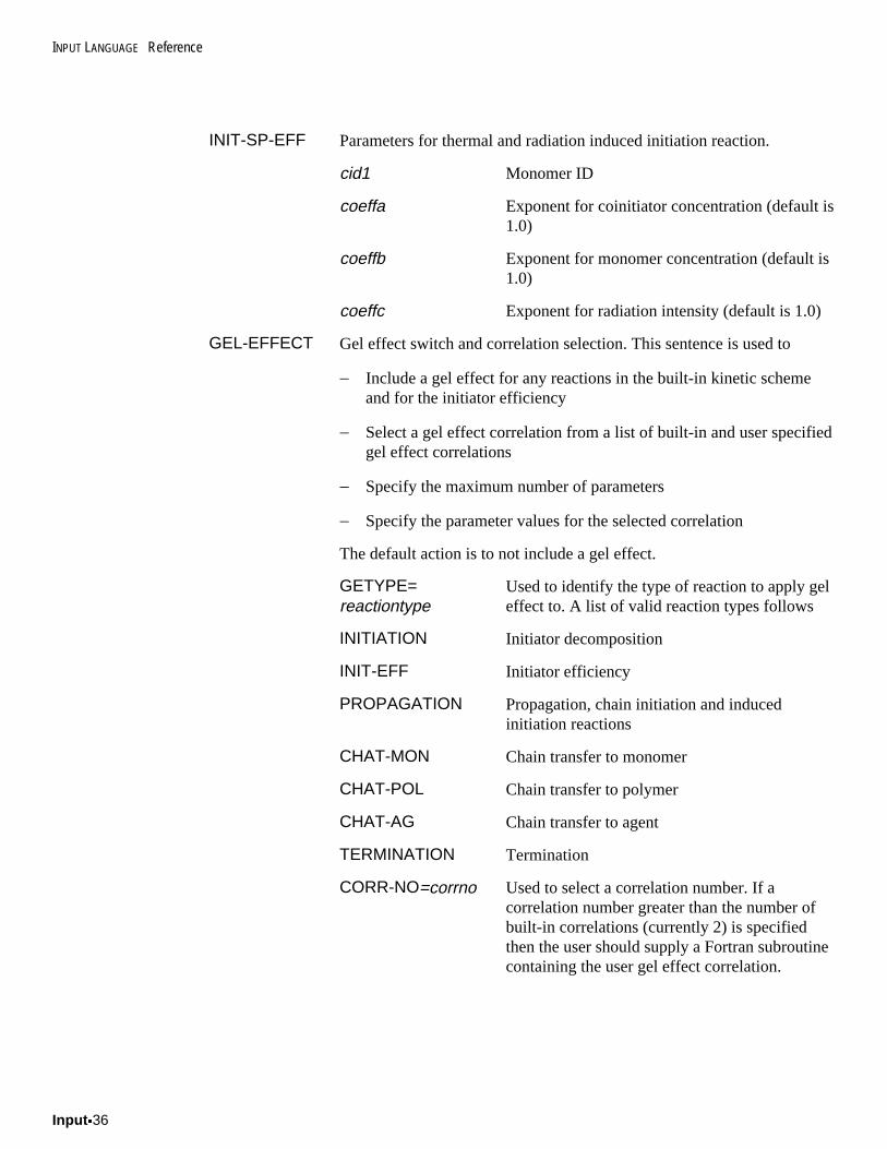
INPUT LANGUAGE Reference
Input x36
INIT-SP-EFF Parameters for thermal and radiation induced initiation reaction.
cid1 Monomer ID
coeffa Exponent for coinitiator concentration (default is1.0)
coeffb Exponent for monomer concentration (default is1.0)
coeffc Exponent for radiation intensity (default is 1.0)
GEL-EFFECT Gel effect switch and correlation selection. This sentence is used to
�� Include a gel effect for any reactions in the built-in kinetic schemeand for the initiator efficiency
�� Select a gel effect correlation from a list of built-in and user specifiedgel effect correlations
�� Specify the maximum number of parameters
�� Specify the parameter values for the selected correlation
The default action is to not include a gel effect.
GETYPE=reactiontype
Used to identify the type of reaction to apply geleffect to. A list of valid reaction types follows
INITIATION Initiator decomposition
INIT-EFF Initiator efficiency
PROPAGATION Propagation, chain initiation and inducedinitiation reactions
CHAT-MON Chain transfer to monomer
CHAT-POL Chain transfer to polymer
CHAT-AG Chain transfer to agent
TERMINATION Termination
CORR-NO=corrno Used to select a correlation number. If acorrelation number greater than the number ofbuilt-in correlations (currently 2) is specifiedthen the user should supply a Fortran subroutinecontaining the user gel effect correlation.
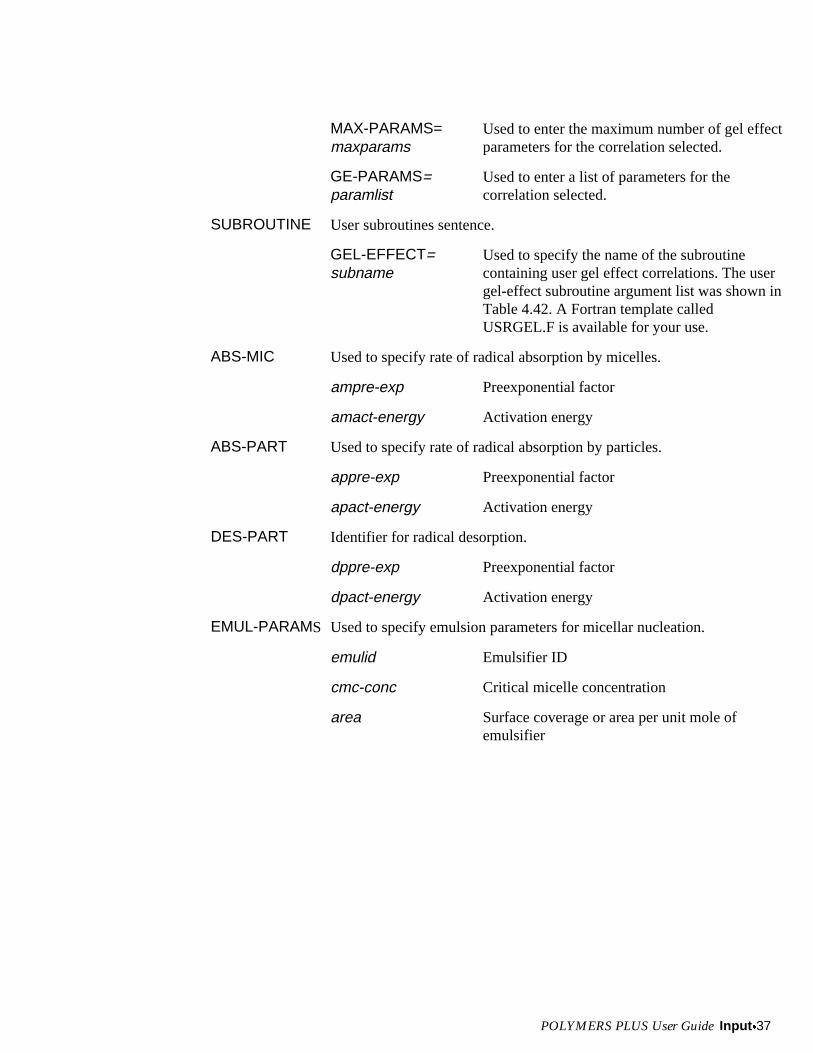
POLYMERS PLUS User Guide Input x37
MAX-PARAMS=maxparams
Used to enter the maximum number of gel effectparameters for the correlation selected.
GE-PARAMS=paramlist
Used to enter a list of parameters for thecorrelation selected.
SUBROUTINE User subroutines sentence.
GEL-EFFECT=subname
Used to specify the name of the subroutinecontaining user gel effect correlations. The usergel-effect subroutine argument list was shown inTable 4.42. A Fortran template calledUSRGEL.F is available for your use.
ABS-MIC Used to specify rate of radical absorption by micelles.
ampre-exp Preexponential factor
amact-energy Activation energy
ABS-PART Used to specify rate of radical absorption by particles.
appre-exp Preexponential factor
apact-energy Activation energy
DES-PART Identifier for radical desorption.
dppre-exp Preexponential factor
dpact-energy Activation energy
EMUL-PARAMS Used to specify emulsion parameters for micellar nucleation.
emulid Emulsifier ID
cmc-conc Critical micelle concentration
area Surface coverage or area per unit mole ofemulsifier
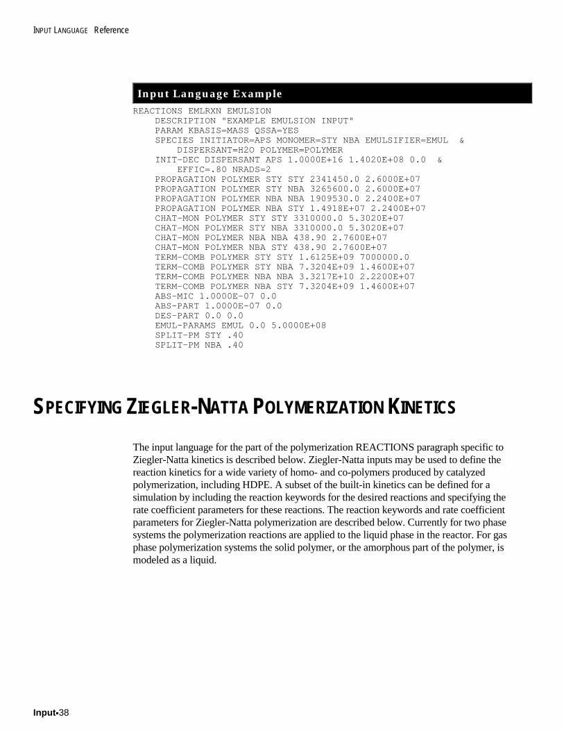
INPUT LANGUAGE Reference
Input x38
Input Language ExampleREACTIONS EMLRXN EMULSION DESCRIPTION "EXAMPLE EMULSION INPUT" PARAM KBASIS=MASS QSSA=YES SPECIES INITIATOR=APS MONOMER=STY NBA EMULSIFIER=EMUL & DISPERSANT=H2O POLYMER=POLYMER INIT-DEC DISPERSANT APS 1.0000E+16 1.4020E+08 0.0 & EFFIC=.80 NRADS=2 PROPAGATION POLYMER STY STY 2341450.0 2.6000E+07 PROPAGATION POLYMER STY NBA 3265600.0 2.6000E+07 PROPAGATION POLYMER NBA NBA 1909530.0 2.2400E+07 PROPAGATION POLYMER NBA STY 1.4918E+07 2.2400E+07 CHAT-MON POLYMER STY STY 3310000.0 5.3020E+07 CHAT-MON POLYMER STY NBA 3310000.0 5.3020E+07 CHAT-MON POLYMER NBA NBA 438.90 2.7600E+07 CHAT-MON POLYMER NBA STY 438.90 2.7600E+07 TERM-COMB POLYMER STY STY 1.6125E+09 7000000.0 TERM-COMB POLYMER STY NBA 7.3204E+09 1.4600E+07 TERM-COMB POLYMER NBA NBA 3.3217E+10 2.2200E+07 TERM-COMB POLYMER NBA STY 7.3204E+09 1.4600E+07 ABS-MIC 1.0000E-07 0.0 ABS-PART 1.0000E-07 0.0 DES-PART 0.0 0.0 EMUL-PARAMS EMUL 0.0 5.0000E+08 SPLIT-PM STY .40 SPLIT-PM NBA .40
SPECIFYING ZIEGLER-NATTA POLYMERIZATION KINETICS
The input language for the part of the polymerization REACTIONS paragraph specific toZiegler-Natta kinetics is described below. Ziegler-Natta inputs may be used to define thereaction kinetics for a wide variety of homo- and co-polymers produced by catalyzedpolymerization, including HDPE. A subset of the built-in kinetics can be defined for asimulation by including the reaction keywords for the desired reactions and specifying therate coefficient parameters for these reactions. The reaction keywords and rate coefficientparameters for Ziegler-Natta polymerization are described below. Currently for two phasesystems the polymerization reactions are applied to the liquid phase in the reactor. For gasphase polymerization systems the solid polymer, or the amorphous part of the polymer, ismodeled as a liquid.
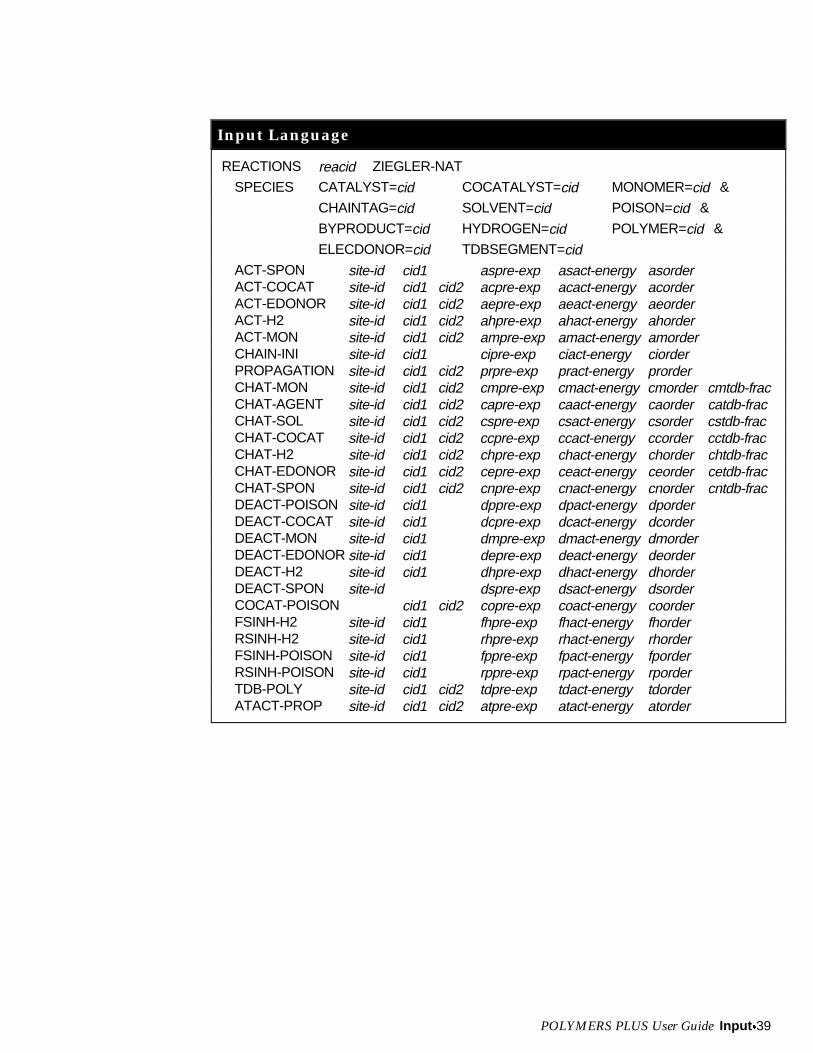
POLYMERS PLUS User Guide Input x39
Input Language
REACTIONS reacid ZIEGLER-NAT
SPECIES CATALYST=cid COCATALYST=cid MONOMER=cid &
CHAINTAG=cid SOLVENT=cid POISON=cid &
BYPRODUCT=cid HYDROGEN=cid POLYMER=cid &
ELECDONOR=cid TDBSEGMENT=cidACT-SPON site-id cid1 aspre-exp asact-energy asorderACT-COCAT site-id cid1 cid2 acpre-exp acact-energy acorderACT-EDONOR site-id cid1 cid2 aepre-exp aeact-energy aeorderACT-H2 site-id cid1 cid2 ahpre-exp ahact-energy ahorderACT-MON site-id cid1 cid2 ampre-exp amact-energy amorderCHAIN-INI site-id cid1 cipre-exp ciact-energy ciorderPROPAGATION site-id cid1 cid2 prpre-exp pract-energy prorderCHAT-MON site-id cid1 cid2 cmpre-exp cmact-energy cmorder cmtdb-fracCHAT-AGENT site-id cid1 cid2 capre-exp caact-energy caorder catdb-fracCHAT-SOL site-id cid1 cid2 cspre-exp csact-energy csorder cstdb-fracCHAT-COCAT site-id cid1 cid2 ccpre-exp ccact-energy ccorder cctdb-fracCHAT-H2 site-id cid1 cid2 chpre-exp chact-energy chorder chtdb-fracCHAT-EDONOR site-id cid1 cid2 cepre-exp ceact-energy ceorder cetdb-fracCHAT-SPON site-id cid1 cid2 cnpre-exp cnact-energy cnorder cntdb-fracDEACT-POISON site-id cid1 dppre-exp dpact-energy dporderDEACT-COCAT site-id cid1 dcpre-exp dcact-energy dcorderDEACT-MON site-id cid1 dmpre-exp dmact-energy dmorderDEACT-EDONOR site-id cid1 depre-exp deact-energy deorderDEACT-H2 site-id cid1 dhpre-exp dhact-energy dhorderDEACT-SPON site-id dspre-exp dsact-energy dsorderCOCAT-POISON cid1 cid2 copre-exp coact-energy coorderFSINH-H2 site-id cid1 fhpre-exp fhact-energy fhorderRSINH-H2 site-id cid1 rhpre-exp rhact-energy rhorderFSINH-POISON site-id cid1 fppre-exp fpact-energy fporderRSINH-POISON site-id cid1 rppre-exp rpact-energy rporderTDB-POLY site-id cid1 cid2 tdpre-exp tdact-energy tdorderATACT-PROP site-id cid1 cid2 atpre-exp atact-energy atorder
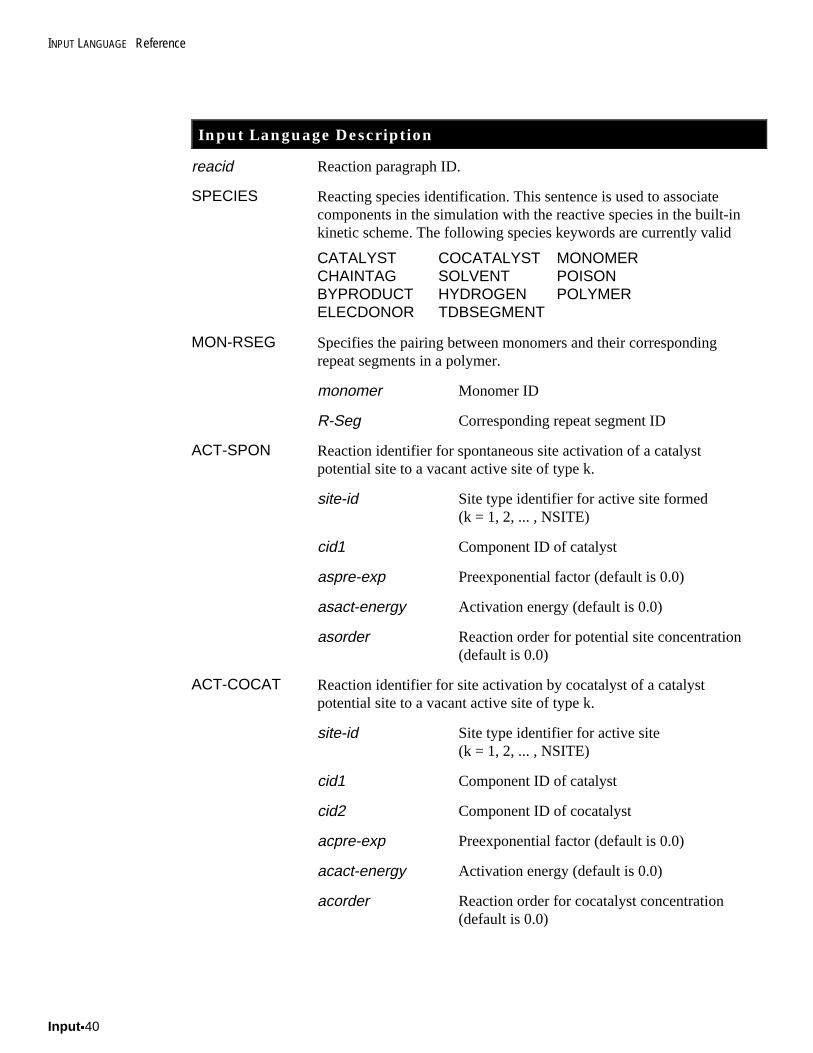
INPUT LANGUAGE Reference
Input x40
Input Language Description
reacid Reaction paragraph ID.
SPECIES Reacting species identification. This sentence is used to associatecomponents in the simulation with the reactive species in the built-inkinetic scheme. The following species keywords are currently valid
CATALYST COCATALYST MONOMERCHAINTAG SOLVENT POISONBYPRODUCT HYDROGEN POLYMERELECDONOR TDBSEGMENT
MON-RSEG Specifies the pairing between monomers and their correspondingrepeat segments in a polymer.
monomer Monomer ID
R-Seg Corresponding repeat segment ID
ACT-SPON Reaction identifier for spontaneous site activation of a catalystpotential site to a vacant active site of type k.
site-id Site type identifier for active site formed(k = 1, 2, ... , NSITE)
cid1 Component ID of catalyst
aspre-exp Preexponential factor (default is 0.0)
asact-energy Activation energy (default is 0.0)
asorder Reaction order for potential site concentration(default is 0.0)
ACT-COCAT Reaction identifier for site activation by cocatalyst of a catalystpotential site to a vacant active site of type k.
site-id Site type identifier for active site(k = 1, 2, ... , NSITE)
cid1 Component ID of catalyst
cid2 Component ID of cocatalyst
acpre-exp Preexponential factor (default is 0.0)
acact-energy Activation energy (default is 0.0)
acorder Reaction order for cocatalyst concentration(default is 0.0)
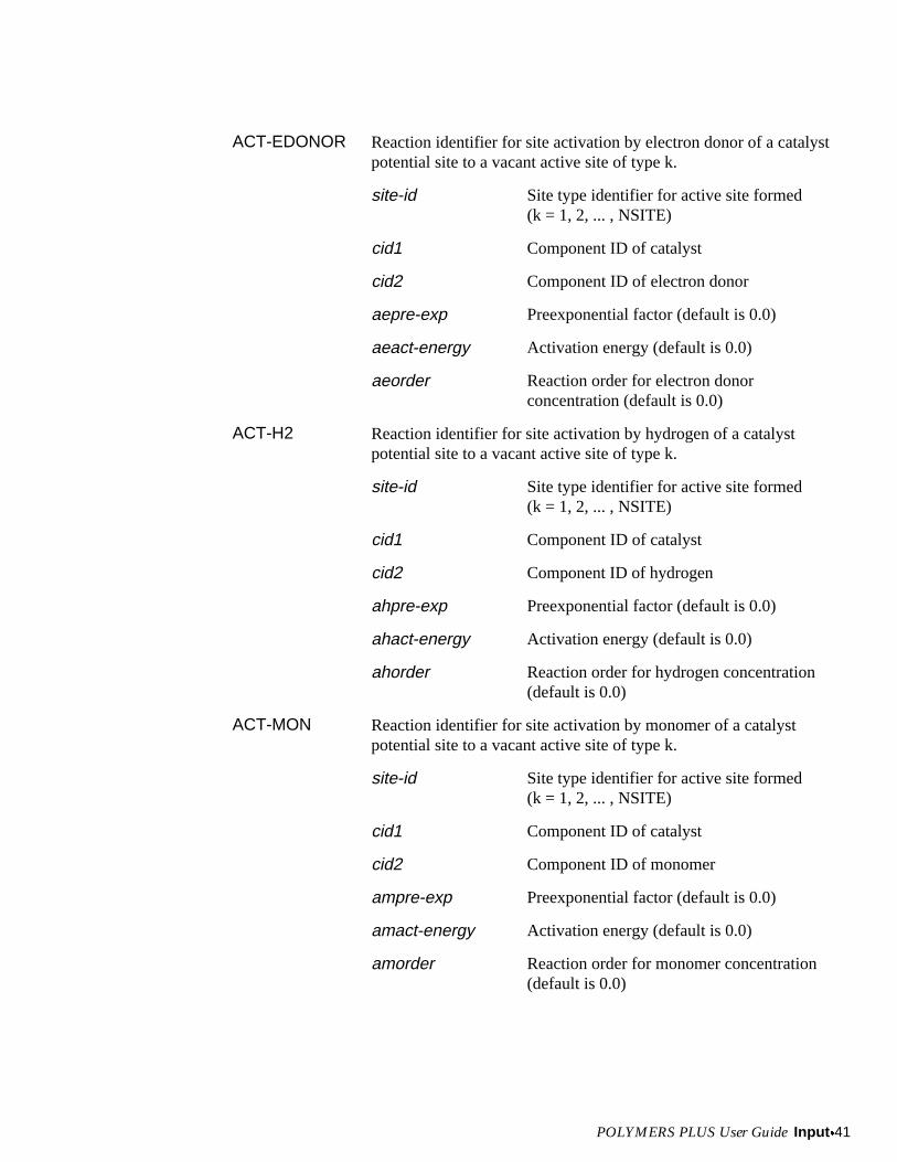
POLYMERS PLUS User Guide Input x41
ACT-EDONOR Reaction identifier for site activation by electron donor of a catalystpotential site to a vacant active site of type k.
site-id Site type identifier for active site formed(k = 1, 2, ... , NSITE)
cid1 Component ID of catalyst
cid2 Component ID of electron donor
aepre-exp Preexponential factor (default is 0.0)
aeact-energy Activation energy (default is 0.0)
aeorder Reaction order for electron donorconcentration (default is 0.0)
ACT-H2 Reaction identifier for site activation by hydrogen of a catalystpotential site to a vacant active site of type k.
site-id Site type identifier for active site formed(k = 1, 2, ... , NSITE)
cid1 Component ID of catalyst
cid2 Component ID of hydrogen
ahpre-exp Preexponential factor (default is 0.0)
ahact-energy Activation energy (default is 0.0)
ahorder Reaction order for hydrogen concentration(default is 0.0)
ACT-MON Reaction identifier for site activation by monomer of a catalystpotential site to a vacant active site of type k.
site-id Site type identifier for active site formed(k = 1, 2, ... , NSITE)
cid1 Component ID of catalyst
cid2 Component ID of monomer
ampre-exp Preexponential factor (default is 0.0)
amact-energy Activation energy (default is 0.0)
amorder Reaction order for monomer concentration(default is 0.0)
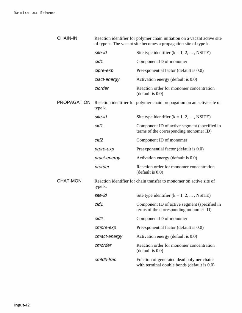
INPUT LANGUAGE Reference
Input x42
CHAIN-INI Reaction identifier for polymer chain initiation on a vacant active siteof type k. The vacant site becomes a propagation site of type k.
site-id Site type identifier (k = 1, 2, ... , NSITE)
cid1 Component ID of monomer
cipre-exp Preexponential factor (default is 0.0)
ciact-energy Activation energy (default is 0.0)
ciorder Reaction order for monomer concentration(default is 0.0)
PROPAGATION Reaction identifier for polymer chain propagation on an active site oftype k.
site-id Site type identifier (k = 1, 2, ... , NSITE)
cid1 Component ID of active segment (specified interms of the corresponding monomer ID)
cid2 Component ID of monomer
prpre-exp Preexponential factor (default is 0.0)
pract-energy Activation energy (default is 0.0)
prorder Reaction order for monomer concentration(default is 0.0)
CHAT-MON Reaction identifier for chain transfer to monomer on active site oftype k.
site-id Site type identifier (k = 1, 2, ... , NSITE)
cid1 Component ID of active segment (specified interms of the corresponding monomer ID)
cid2 Component ID of monomer
cmpre-exp Preexponential factor (default is 0.0)
cmact-energy Activation energy (default is 0.0)
cmorder Reaction order for monomer concentration(default is 0.0)
cmtdb-frac Fraction of generated dead polymer chainswith terminal double bonds (default is 0.0)
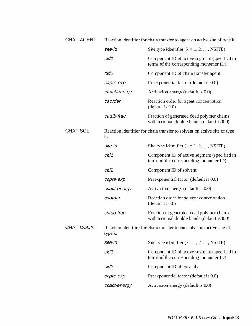
POLYMERS PLUS User Guide Input x43
CHAT-AGENT Reaction identifier for chain transfer to agent on active site of type k.
site-id Site type identifier (k = 1, 2, ... , NSITE)
cid1 Component ID of active segment (specified interms of the corresponding monomer ID)
cid2 Component ID of chain transfer agent
capre-exp Preexponential factor (default is 0.0)
caact-energy Activation energy (default is 0.0)
caorder Reaction order for agent concentration(default is 0.0)
catdb-frac Fraction of generated dead polymer chainswith terminal double bonds (default is 0.0)
CHAT-SOL Reaction identifier for chain transfer to solvent on active site of typek.
site-id Site type identifier (k = 1, 2, ... , NSITE)
cid1 Component ID of active segment (specified interms of the corresponding monomer ID)
cid2 Component ID of solvent
cspre-exp Preexponential factor (default is 0.0)
csact-energy Activation energy (default is 0.0)
csorder Reaction order for solvent concentration(default is 0.0)
cstdb-frac Fraction of generated dead polymer chainswith terminal double bonds (default is 0.0)
CHAT-COCAT Reaction identifier for chain transfer to cocatalyst on active site oftype k.
site-id Site type identifier (k = 1, 2, ... , NSITE)
cid1 Component ID of active segment (specified interms of the corresponding monomer ID)
cid2 Component ID of cocatalyst
ccpre-exp Preexponential factor (default is 0.0)
ccact-energy Activation energy (default is 0.0)
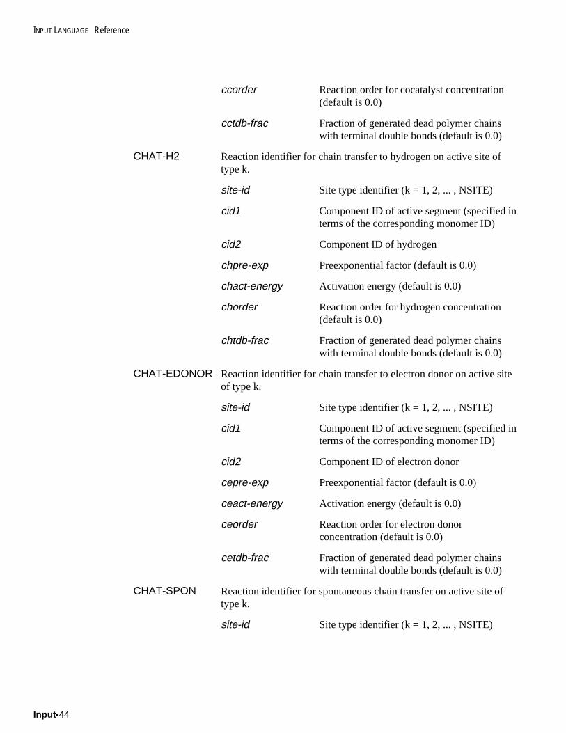
INPUT LANGUAGE Reference
Input x44
ccorder Reaction order for cocatalyst concentration(default is 0.0)
cctdb-frac Fraction of generated dead polymer chainswith terminal double bonds (default is 0.0)
CHAT-H2 Reaction identifier for chain transfer to hydrogen on active site oftype k.
site-id Site type identifier (k = 1, 2, ... , NSITE)
cid1 Component ID of active segment (specified interms of the corresponding monomer ID)
cid2 Component ID of hydrogen
chpre-exp Preexponential factor (default is 0.0)
chact-energy Activation energy (default is 0.0)
chorder Reaction order for hydrogen concentration(default is 0.0)
chtdb-frac Fraction of generated dead polymer chainswith terminal double bonds (default is 0.0)
CHAT-EDONOR Reaction identifier for chain transfer to electron donor on active siteof type k.
site-id Site type identifier (k = 1, 2, ... , NSITE)
cid1 Component ID of active segment (specified interms of the corresponding monomer ID)
cid2 Component ID of electron donor
cepre-exp Preexponential factor (default is 0.0)
ceact-energy Activation energy (default is 0.0)
ceorder Reaction order for electron donorconcentration (default is 0.0)
cetdb-frac Fraction of generated dead polymer chainswith terminal double bonds (default is 0.0)
CHAT-SPON Reaction identifier for spontaneous chain transfer on active site oftype k.
site-id Site type identifier (k = 1, 2, ... , NSITE)
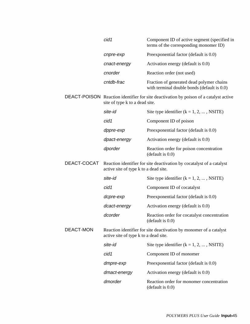
POLYMERS PLUS User Guide Input x45
cid1 Component ID of active segment (specified interms of the corresponding monomer ID)
cnpre-exp Preexponential factor (default is 0.0)
cnact-energy Activation energy (default is 0.0)
cnorder Reaction order (not used)
cntdb-frac Fraction of generated dead polymer chainswith terminal double bonds (default is 0.0)
DEACT-POISON Reaction identifier for site deactivation by poison of a catalyst activesite of type k to a dead site.
site-id Site type identifier (k = 1, 2, ... , NSITE)
cid1 Component ID of poison
dppre-exp Preexponential factor (default is 0.0)
dpact-energy Activation energy (default is 0.0)
dporder Reaction order for poison concentration(default is 0.0)
DEACT-COCAT Reaction identifier for site deactivation by cocatalyst of a catalystactive site of type k to a dead site.
site-id Site type identifier (k = 1, 2, ... , NSITE)
cid1 Component ID of cocatalyst
dcpre-exp Preexponential factor (default is 0.0)
dcact-energy Activation energy (default is 0.0)
dcorder Reaction order for cocatalyst concentration(default is 0.0)
DEACT-MON Reaction identifier for site deactivation by monomer of a catalystactive site of type k to a dead site.
site-id Site type identifier (k = 1, 2, ... , NSITE)
cid1 Component ID of monomer
dmpre-exp Preexponential factor (default is 0.0)
dmact-energy Activation energy (default is 0.0)
dmorder Reaction order for monomer concentration(default is 0.0)
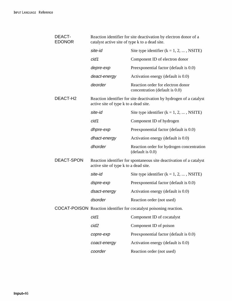
INPUT LANGUAGE Reference
Input x46
DEACT-EDONOR
Reaction identifier for site deactivation by electron donor of acatalyst active site of type k to a dead site.
site-id Site type identifier (k = 1, 2, ... , NSITE)
cid1 Component ID of electron donor
depre-exp Preexponential factor (default is 0.0)
deact-energy Activation energy (default is 0.0)
deorder Reaction order for electron donorconcentration (default is 0.0)
DEACT-H2 Reaction identifier for site deactivation by hydrogen of a catalystactive site of type k to a dead site.
site-id Site type identifier (k = 1, 2, ... , NSITE)
cid1 Component ID of hydrogen
dhpre-exp Preexponential factor (default is 0.0)
dhact-energy Activation energy (default is 0.0)
dhorder Reaction order for hydrogen concentration(default is 0.0)
DEACT-SPON Reaction identifier for spontaneous site deactivation of a catalystactive site of type k to a dead site.
site-id Site type identifier (k = 1, 2, ... , NSITE)
dspre-exp Preexponential factor (default is 0.0)
dsact-energy Activation energy (default is 0.0)
dsorder Reaction order (not used)
COCAT-POISON Reaction identifier for cocatalyst poisoning reaction.
cid1 Component ID of cocatalyst
cid2 Component ID of poison
copre-exp Preexponential factor (default is 0.0)
coact-energy Activation energy (default is 0.0)
coorder Reaction order (not used)
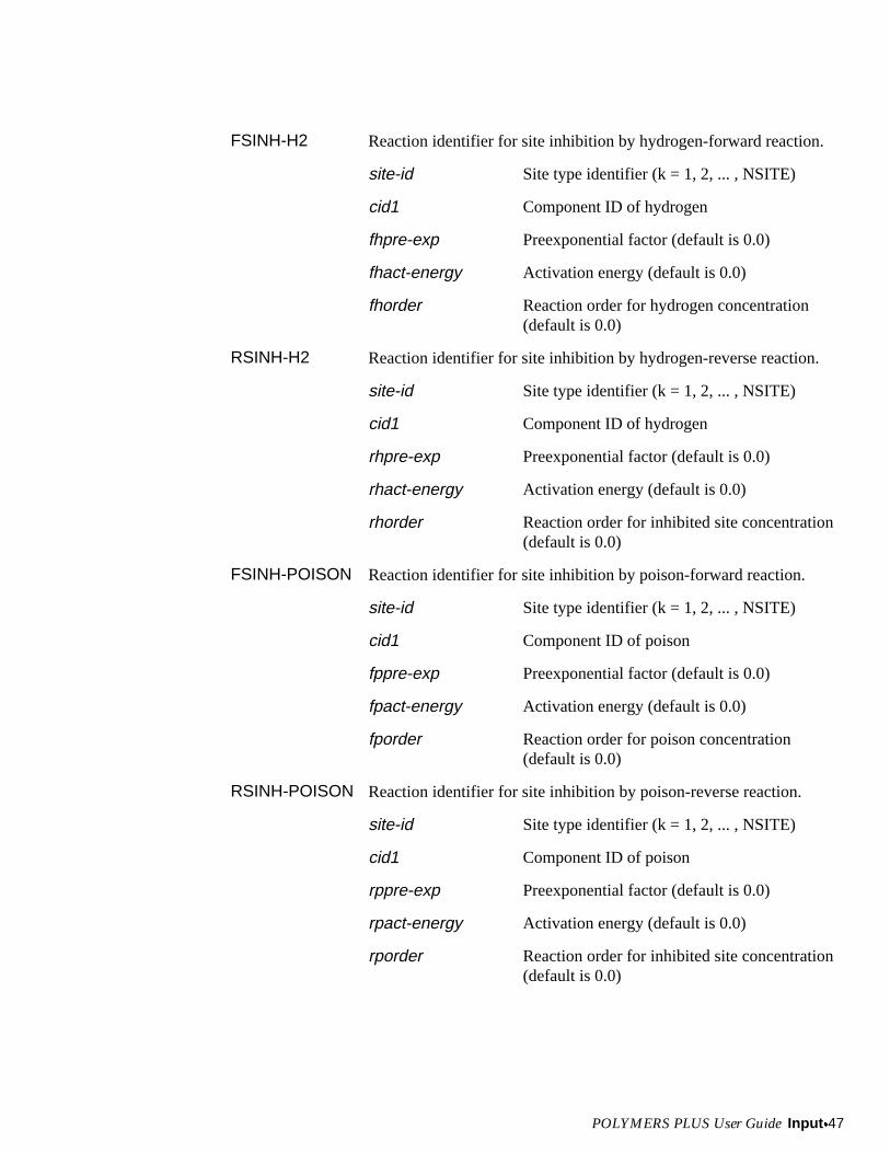
POLYMERS PLUS User Guide Input x47
FSINH-H2 Reaction identifier for site inhibition by hydrogen-forward reaction.
site-id Site type identifier (k = 1, 2, ... , NSITE)
cid1 Component ID of hydrogen
fhpre-exp Preexponential factor (default is 0.0)
fhact-energy Activation energy (default is 0.0)
fhorder Reaction order for hydrogen concentration(default is 0.0)
RSINH-H2 Reaction identifier for site inhibition by hydrogen-reverse reaction.
site-id Site type identifier (k = 1, 2, ... , NSITE)
cid1 Component ID of hydrogen
rhpre-exp Preexponential factor (default is 0.0)
rhact-energy Activation energy (default is 0.0)
rhorder Reaction order for inhibited site concentration(default is 0.0)
FSINH-POISON Reaction identifier for site inhibition by poison-forward reaction.
site-id Site type identifier (k = 1, 2, ... , NSITE)
cid1 Component ID of poison
fppre-exp Preexponential factor (default is 0.0)
fpact-energy Activation energy (default is 0.0)
fporder Reaction order for poison concentration(default is 0.0)
RSINH-POISON Reaction identifier for site inhibition by poison-reverse reaction.
site-id Site type identifier (k = 1, 2, ... , NSITE)
cid1 Component ID of poison
rppre-exp Preexponential factor (default is 0.0)
rpact-energy Activation energy (default is 0.0)
rporder Reaction order for inhibited site concentration(default is 0.0)
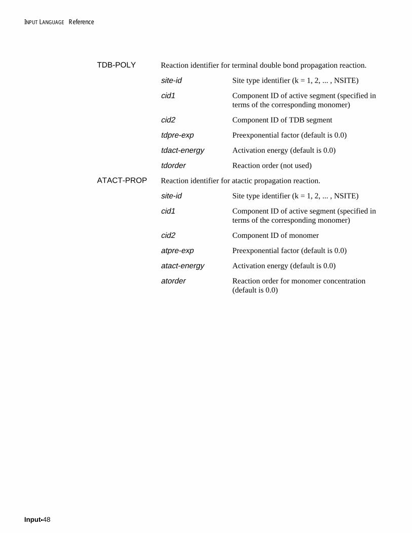
INPUT LANGUAGE Reference
Input x48
TDB-POLY Reaction identifier for terminal double bond propagation reaction.
site-id Site type identifier (k = 1, 2, ... , NSITE)
cid1 Component ID of active segment (specified interms of the corresponding monomer)
cid2 Component ID of TDB segment
tdpre-exp Preexponential factor (default is 0.0)
tdact-energy Activation energy (default is 0.0)
tdorder Reaction order (not used)
ATACT-PROP Reaction identifier for atactic propagation reaction.
site-id Site type identifier (k = 1, 2, ... , NSITE)
cid1 Component ID of active segment (specified interms of the corresponding monomer)
cid2 Component ID of monomer
atpre-exp Preexponential factor (default is 0.0)
atact-energy Activation energy (default is 0.0)
atorder Reaction order for monomer concentration(default is 0.0)
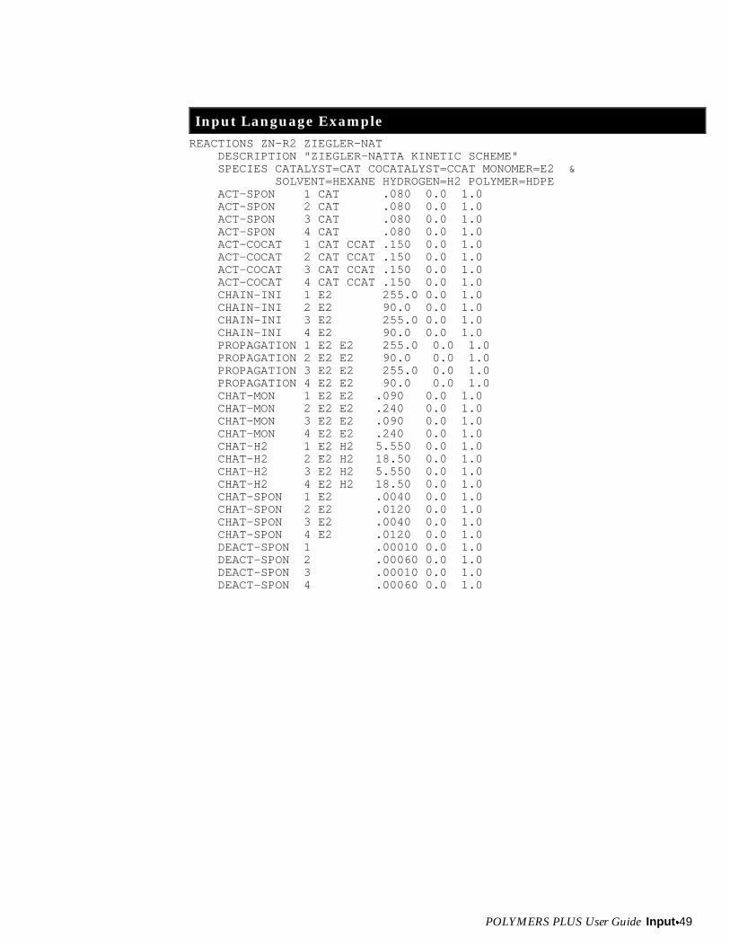
POLYMERS PLUS User Guide Input x49
Input Language ExampleREACTIONS ZN-R2 ZIEGLER-NAT DESCRIPTION "ZIEGLER-NATTA KINETIC SCHEME" SPECIES CATALYST=CAT COCATALYST=CCAT MONOMER=E2 & SOLVENT=HEXANE HYDROGEN=H2 POLYMER=HDPE ACT-SPON 1 CAT .080 0.0 1.0 ACT-SPON 2 CAT .080 0.0 1.0 ACT-SPON 3 CAT .080 0.0 1.0 ACT-SPON 4 CAT .080 0.0 1.0 ACT-COCAT 1 CAT CCAT .150 0.0 1.0 ACT-COCAT 2 CAT CCAT .150 0.0 1.0 ACT-COCAT 3 CAT CCAT .150 0.0 1.0 ACT-COCAT 4 CAT CCAT .150 0.0 1.0 CHAIN-INI 1 E2 255.0 0.0 1.0 CHAIN-INI 2 E2 90.0 0.0 1.0 CHAIN-INI 3 E2 255.0 0.0 1.0 CHAIN-INI 4 E2 90.0 0.0 1.0 PROPAGATION 1 E2 E2 255.0 0.0 1.0 PROPAGATION 2 E2 E2 90.0 0.0 1.0 PROPAGATION 3 E2 E2 255.0 0.0 1.0 PROPAGATION 4 E2 E2 90.0 0.0 1.0 CHAT-MON 1 E2 E2 .090 0.0 1.0 CHAT-MON 2 E2 E2 .240 0.0 1.0 CHAT-MON 3 E2 E2 .090 0.0 1.0 CHAT-MON 4 E2 E2 .240 0.0 1.0 CHAT-H2 1 E2 H2 5.550 0.0 1.0 CHAT-H2 2 E2 H2 18.50 0.0 1.0 CHAT-H2 3 E2 H2 5.550 0.0 1.0 CHAT-H2 4 E2 H2 18.50 0.0 1.0 CHAT-SPON 1 E2 .0040 0.0 1.0 CHAT-SPON 2 E2 .0120 0.0 1.0 CHAT-SPON 3 E2 .0040 0.0 1.0 CHAT-SPON 4 E2 .0120 0.0 1.0 DEACT-SPON 1 .00010 0.0 1.0 DEACT-SPON 2 .00060 0.0 1.0 DEACT-SPON 3 .00010 0.0 1.0 DEACT-SPON 4 .00060 0.0 1.0
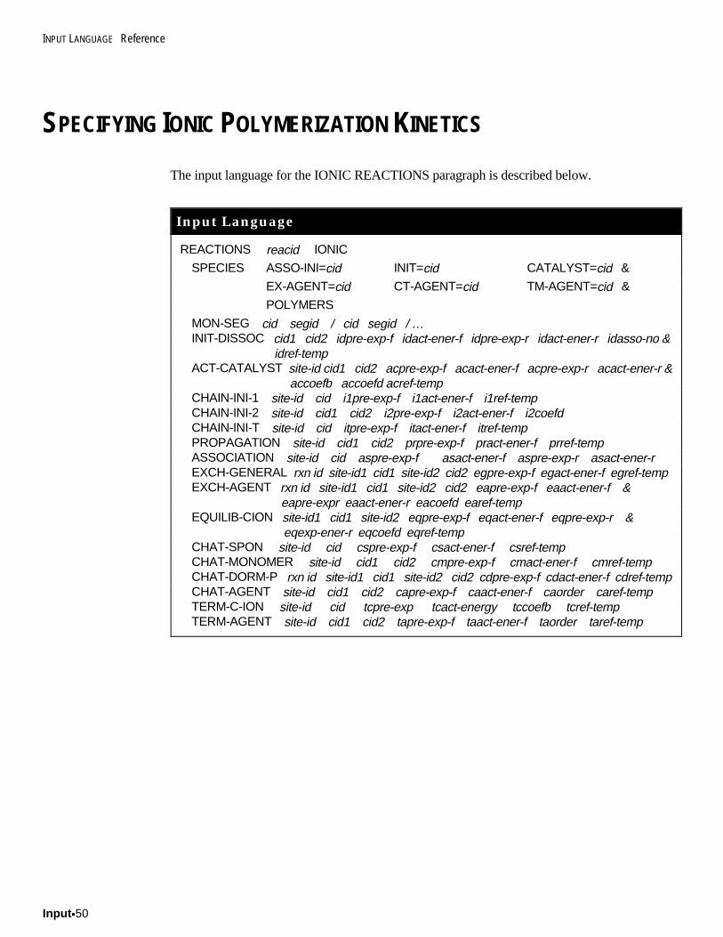
INPUT LANGUAGE Reference
Input x50
SPECIFYING IONIC POLYMERIZATION KINETICS
The input language for the IONIC REACTIONS paragraph is described below.
Input Language
REACTIONS reacid IONIC
SPECIES ASSO-INI=cid INIT=cid CATALYST=cid &
EX-AGENT=cid CT-AGENT=cid TM-AGENT=cid &
POLYMERS
MON-SEG cid segid / cid segid / …INIT-DISSOC cid1 cid2 idpre-exp-f idact-ener-f idpre-exp-r idact-ener-r idasso-no &
idref-tempACT-CATALYST site-id cid1 cid2 acpre-exp-f acact-ener-f acpre-exp-r acact-ener-r &
accoefb accoefd acref-tempCHAIN-INI-1 site-id cid i1pre-exp-f i1act-ener-f i1ref-tempCHAIN-INI-2 site-id cid1 cid2 i2pre-exp-f i2act-ener-f i2coefdCHAIN-INI-T site-id cid itpre-exp-f itact-ener-f itref-tempPROPAGATION site-id cid1 cid2 prpre-exp-f pract-ener-f prref-tempASSOCIATION site-id cid aspre-exp-f asact-ener-f aspre-exp-r asact-ener-rEXCH-GENERAL rxn id site-id1 cid1 site-id2 cid2 egpre-exp-f egact-ener-f egref-tempEXCH-AGENT rxn id site-id1 cid1 site-id2 cid2 eapre-exp-f eaact-ener-f &
eapre-expr eaact-ener-r eacoefd earef-tempEQUILIB-CION site-id1 cid1 site-id2 eqpre-exp-f eqact-ener-f eqpre-exp-r &
eqexp-ener-r eqcoefd eqref-tempCHAT-SPON site-id cid cspre-exp-f csact-ener-f csref-tempCHAT-MONOMER site-id cid1 cid2 cmpre-exp-f cmact-ener-f cmref-tempCHAT-DORM-P rxn id site-id1 cid1 site-id2 cid2 cdpre-exp-f cdact-ener-f cdref-tempCHAT-AGENT site-id cid1 cid2 capre-exp-f caact-ener-f caorder caref-tempTERM-C-ION site-id cid tcpre-exp tcact-energy tccoefb tcref-tempTERM-AGENT site-id cid1 cid2 tapre-exp-f taact-ener-f taorder taref-temp
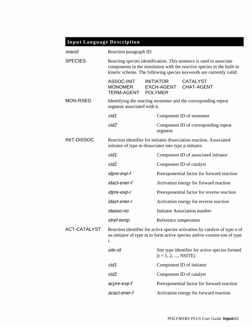
POLYMERS PLUS User Guide Input x51
Input Language Description
reacid Reaction paragraph ID.
SPECIES Reacting species identification. This sentence is used to associatecomponents in the simulation with the reactive species in the built-inkinetic scheme. The following species keywords are currently valid:
ASSOC-INIT INITIATOR CATALYSTMONOMER EXCH-AGENT CHAT-AGENTTERM-AGENT POLYMER
MON-RSEG Identifying the reacting monomer and the corresponding repeatsegment associated with it.
cid1 Component ID of monomer
cid2 Component ID of corresponding repeatsegment
INIT-DISSOC Reaction identifier for initiator dissociation reaction. Associatedinitiator of type m dissociates into type p initiator.
cid1 Component ID of associated initiator
cid2 Component ID of catalyst
idpre-exp-f Preexponential factor for forward reaction
idact-ener-f Activation energy for forward reaction
idpre-exp-r Preexponential factor for reverse reaction
idact-ener-r Activation energy for reverse reaction
idasso-no Initiator Association number
idref-temp Reference temperature
ACT-CATALYST Reaction identifier for active species activation by catalyst of type n ofan initiator of type m to form active species and/or counter-ion of typei.
site-id Site type identifier for active species formed(i = 1, 2, ..., NSITE)
cid1 Component ID of initiator
cid2 Component ID of catalyst
acpre-exp-f Preexponential factor for forward reaction
acact-ener-f Activation energy for forward reaction
INPUT LANGUAGE Reference
Input x52
acpre-exp-r Preexponential factor for reverse reaction
acact-ener-r Activation energy for reverse reaction
accoefb 0 if cid2 does not participate in the reaction.1 if cid2 participates in the reaction
accoefd 0 if counter-ion is absent. 1 if counter-ion ispresent
acref-temp Reference temperature
CHAIN-INI-1 Reaction identifier for chain initiation of active species of type i bymonomer of type j.
site-id Site type identifier for active species formed(i = 1, 2, ..., NSITE)
cid Component ID of monomer
i1pre-exp-f Preexponential factor
i1act-ener-f Activation energy
i1ref-temp Reference temperature
CHAIN-INI-2 Reaction identifier for chain initiation of active species of type i bymonomer of type j reacting with initiator of type m.
site-id Site type identifier for active species formed(i = 1, 2, ..., NSITE)
cid1 Component ID of initiator
cid2 Component ID of monomer
i2pre-exp-f Preexponential factor
i2act-ener-f Activation energy
i2coefd 1 if counter-ion is formed. 0 otherwise
tref Reference temperature
CHAIN-INI-T Reaction identifier for chain initiation of transfer active species of typei by monomer of type j.
site-id Site type identifier for active species formed(i = 1, 2, ..., NSITE)
cid Component ID of monomer
itpre-exp-f Preexponential factor
POLYMERS PLUS User Guide Input x53
itact-ener-f Activation energy
itref-temp Reference temperature
PROPAGATION Reaction identifier for polymer chain propagation on an active speciesof type i.
site-id Site type identifier for active species formed(i = 1, 2, ..., NSITE)
cid1 Component ID of active segment
cid2 Component ID of monomer
prpre-exp-f Preexponential factor
pract-ener-f Activation energy
prref-temp Reference temperature
ASSOCIATION Reaction identifier for polymer association with active species of typei.
site-id Site type identifier for active species formed(i = 1, 2, ..., NSITE)
cid Component ID of active segment
aspre-exp-f Preexponential factor for forward reaction(forming aggregate polymer)
asact-ener-f Activation energy for forward reaction
aspre-exp-r Preexponential factor for reverse reaction
asact-ener-r Activation energy for reverse reaction
asasso-no Polymer association
asref-temp Reference temperature
EXCH-GENERAL Reaction identifier for general exchange reaction between twogrowing polymer chains with unique active species and end segmentsattached to them.
rxn id Reaction ID for a unique rate constant
site-id1 Site type identifier for first active species(i = 1, 2, ... , NSITE)
cid1 Component ID of active segment on siteid1
INPUT LANGUAGE Reference
Input x54
site-id2 Site type identifier for second active species(i = 1, 2, ... , NSITE)
cid2 Component ID of active segment on siteid2
egpre-exp-f Preexponential factor
egact-ener-f Activation energy
egref-temp Reference temperature
EXCH-AGENT Reaction identifier for exchange between growing i polymer specieswith k segment attached to it and an exchange-agent of type m.
rxn id Reaction ID for a unique rate constant
site-id1 Site type identifier for first active species(i = 1, 2, ... , NSITE)
cid1 Component ID of active segment on siteid1
site-id2 Site type identifier for second active species(i = 1, 2, ... , NSITE) formed
cid2 Component ID of exchange agent
eapre-exp-f Preexponential factor for forward reaction
eaact-ener-f Activation energy for forward reaction
eapre-exp-r Preexponential factor for reverse reaction
eaact-ener-r Activation energy for reverse reaction
eacoefd 0 if Po is absent. 1 if Po is present
earef-temp Reference temperature
EQUILIB-CION Reaction identifier for equilibrium with counter-ion between i and jactive species with kth segment attached to it.
site-id1 Site type identifier for first active species(i = 1, 2, ... , NSITE)
cid Component ID of active segment
site-id2 Site type identifier for second active species(j = 1, 2, ... , NSITE)
eqpre-exp-f Preexponential factor for forward reaction
eqact-ener-f Activation energy for forward reaction
POLYMERS PLUS User Guide Input x55
eqpre-exp-r Preexponential factor for reverse reaction
eqact-ener-r Activation energy for reverse reaction
eqcoefd 0 if counter-ion is absent. 1 if counter-ion ispresent
eqref-temp Reference temperature
CHAT-SPON Reaction identifier for spontaneous chain transfer on active species oftype i.
site-id Site type identifier for active species(i=1, 2, ... , NSITE)
cid Component ID of active segment
cspre-exp-f Preexponential factor
csact-ener-f Activation energy
csref-temp Reference temperature
CHAT-MONOMER Reaction identifier for chain transfer to monomer of type j on activespecies of type i.
site-id Site type identifier for active species(i=1, 2, ... , NSITE)
cid1 Component ID of active segment
cid2 Component ID of monomer
cmpre-exp-f Preexponential factor
cmact-ener-f Activation energy
cmref-temp Reference temperature
CHAT-DORM-P Reaction identifier for chain transfer on active species of type i to formdormant polymer of type j.
rxn id Reaction ID for a unique rate constant
site-id1 Site type identifier for growing active species(i = 1, 2, ... , NSITE)
cid1 Component ID of active segment on siteid1
site-id2 Site type identifier for product active species(j = 1, 2, ... , NSITE) formed
cid2 Component ID of monomer
INPUT LANGUAGE Reference
Input x56
cdpre-exp-f Preexponential factor
cdact-ener-f Activation energy
cdref-temp Reference temperature
CHAT-AGENT Reaction identifier for chain transfer to chain transfer agent on activespecies of type i.
site-id Site type identifier for active species(i=1, 2, ... , NSITE)
cid1 Component ID of active segment
cid2 Component ID of chain transfer agent
capre-exp-f Preexponential factor
caact-ener-f Activation energy
caorder Reaction order for chain transfer agentconcentration
caref-temp Reference temperature
TERM-C-ION Reaction identifier for chain termination with counter-ion.
site-id Site type identifier for active species(i=1, 2, ... , NSITE)
cid Component ID of active segment
tcpre-exp Preexponential factor
tcact-energy Activation energy
tcoefb 0 if counter-ion does not participate in thereaction. 1 if it does
tcref-temp Reference temperature
TERM-AGENT Reaction identifier for termination with terminating agent.
site-id Site type identifier (i = 1, 2, ... , NSITE)
cid1 Component ID of active agent
cid2 Component ID of terminating agent
tapre-exp-f Preexponential factor
taact-ener-f Activation energy
POLYMERS PLUS User Guide Input x57
taorder Reaction order for terminating agentconcentration
taref-temp Reference temperature
Input Language ExampleREACTIONS R-ION IONIC DESCRIPTION "IONIC KINETIC SCHEME" SPECIES ASSOC-INIT=BULI-3 INITIATOR=BULI-1 POLYMER=PS MON-RSEG STYRENE STY-SEG INIT-DISSOC BULI-3 BULI-1 1.0 0. 2.715E10 0. 3 CHAIN-INI-2 1 BULI-1 STYRENE 0.2055E-2 0. 1 CHAIN-INI-2 2 BULI-1 STYRENE 0.2055E0 0. 0 PROPAGATION 1 STY-SEG STYRENE 0.2055 0. ASSOCIATION 2 STY-SEG 149.7 0 1.0 0 2 EQUILIB-CION 2 STY-SEG 1 1E-3 0. 1.0 0. 1
INPUT LANGUAGE Reference
Input x58
SPECIFYING SEGMENT-BASED POLYMER MODIFICATIONREACTIONS
The input language for the SEGMENT-BAS REACTIONS paragraph is described here.
Input Language
REACTIONS rxnid SEGMENT-BASDESCRIPTION '...'PARAM T-REFERENCE=value PHASE=V/L/L1/L2 CBASIS=basisSPECIES POLYMER=polymeridSTOIC reactionno compid coef / ...RATE-CON reactionno pre-exp act-energy [t-exp] / ...POWLAW-EXP reactionno compid exponent /
The keywords for specifying rate constant parameters, reaction stoichiometry, reactingpolymer, are described below.
Input Language Description
reacid Unique paragraph ID.
DESCRIPTION Up to 64 characters between double quotes.
PARAM Used to enter reaction specifications.
T-REFERENCE=value Reference temperature. If no referencetemperature is given, the term 1/Tref isdropped from the rate expression shown inEquation 4.48.
PHASE=V/L/L1/L2 Reacting phase
CBASIS Basis for power law rate expression. Choicesare as follows
MOLARITY MOLALITY MOLEFRACMASSFRAC MASSCONC
SPECIES Used to specify reacting polymer.
POLYMER=polymerid Polymer component ID (for reacting polymer)
POLYMERS PLUS User Guide Input x59
STOIC Used to specify stoichiometry for user reactions.
reactionno Reaction number
compid Component ID
coef Stoichiometric coefficient (negative forreactants and positive for products)
RATE-CON Used to specify rate constant parameters.
reactionno Reaction number
pre-exp Pre-exponential factor in SI units
act-energy Activation energy in mole enthalpy units
t-exp Temperature exponent
POWLAW-EXP Used to specify power-law exponents.
reactionno Reaction number
compid Component ID
exponent Power law exponent
Input Language ExampleREACTIONS R-1 SEGMENT-BAS PARAM CBASIS=MOLEFRAC SPECIES POLYMER=PVAC STOIC 1 VAC-SEG -1 / H2O -1 / VOH-SEG 1 / ACETIC 1 RATE-CON 1 .001 POWLAW-EXP 1 VAC-SEG 1 / H2O 1 / VOH-SEG 0 / ACETIC 0

INPUT LANGUAGE Reference
Input x60
REFERENCES
Aspen Plus Reference Manual, "Physical Property Data," Aspen Technology, Inc. (1998).
Aspen Plus Reference Manual, "User Models," Aspen Technology, Inc. (1998).
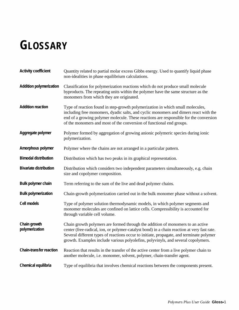
Polymers Plus User Guide Gloss x1
GLOSSARY
Activity coefficient Quantity related to partial molar excess Gibbs energy. Used to quantify liquid phasenon-idealities in phase equilibrium calculations.
Addition polymerization Classification for polymerization reactions which do not produce small moleculebyproducts. The repeating units within the polymer have the same structure as themonomers from which they are originated.
Addition reaction Type of reaction found in step-growth polymerization in which small molecules,including free monomers, dyadic salts, and cyclic monomers and dimers react with theend of a growing polymer molecule. These reactions are responsible for the conversionof the monomers and most of the conversion of functional end groups.
Aggregate polymer Polymer formed by aggregation of growing anionic polymeric species during ionicpolymerization.
Amorphous polymer Polymer where the chains are not arranged in a particular pattern.
Bimodal distribution Distribution which has two peaks in its graphical representation.
Bivariate distribution Distribution which considers two independent parameters simultaneously, e.g. chainsize and copolymer composition.
Bulk polymer chain Term referring to the sum of the live and dead polymer chains.
Bulk polymerization Chain-growth polymerization carried out in the bulk monomer phase without a solvent.
Cell models Type of polymer solution thermodynamic models, in which polymer segments andmonomer molecules are confined on lattice cells. Compressibility is accounted forthrough variable cell volume.
Chain growthpolymerization
Chain growth polymers are formed through the addition of monomers to an activecenter (free-radical, ion, or polymer-catalyst bond) in a chain reaction at very fast rate.Several different types of reactions occur to initiate, propagate, and terminate polymergrowth. Examples include various polyolefins, polyvinyls, and several copolymers.
Chain-transfer reaction Reaction that results in the transfer of the active center from a live polymer chain toanother molecule, i.e. monomer, solvent, polymer, chain-transfer agent.
Chemical equilibria Type of equilibria that involves chemical reactions between the components present.
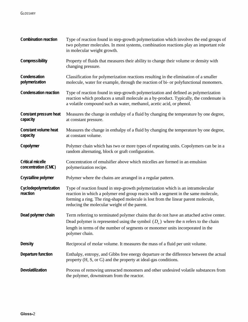
GLOSSARY
Gloss x2
Combination reaction Type of reaction found in step-growth polymerization which involves the end groups oftwo polymer molecules. In most systems, combination reactions play an important rolein molecular weight growth.
Compressibility Property of fluids that measures their ability to change their volume or density withchanging pressure.
Condensationpolymerization
Classification for polymerization reactions resulting in the elimination of a smallermolecule, water for example, through the reaction of bi- or polyfunctional monomers.
Condensation reaction Type of reaction found in step-growth polymerization and defined as polymerizationreaction which produces a small molecule as a by-product. Typically, the condensate isa volatile compound such as water, methanol, acetic acid, or phenol.
Constant pressure heatcapacity
Measures the change in enthalpy of a fluid by changing the temperature by one degree,at constant pressure.
Constant volume heatcapacity
Measures the change in enthalpy of a fluid by changing the temperature by one degree,at constant volume.
Copolymer Polymer chain which has two or more types of repeating units. Copolymers can be in arandom alternating, block or graft configuration.
Critical micelleconcentration (CMC)
Concentration of emulsifier above which micelles are formed in an emulsionpolymerization recipe.
Crystalline polymer Polymer where the chains are arranged in a regular pattern.
Cyclodepolymerizationreaction
Type of reaction found in step-growth polymerization which is an intramolecularreaction in which a polymer end group reacts with a segment in the same molecule,forming a ring. The ring-shaped molecule is lost from the linear parent molecule,reducing the molecular weight of the parent.
Dead polymer chain Term referring to terminated polymer chains that do not have an attached active center.Dead polymer is represented using the symbol ( )Dn where the n refers to the chainlength in terms of the number of segments or monomer units incorporated in thepolymer chain.
Density Reciprocal of molar volume. It measures the mass of a fluid per unit volume.
Departure function Enthalpy, entropy, and Gibbs free energy departure or the difference between the actualproperty (H, S, or G) and the property at ideal-gas conditions.
Devolatilization Process of removing unreacted monomers and other undesired volatile substances fromthe polymer, downstream from the reactor.
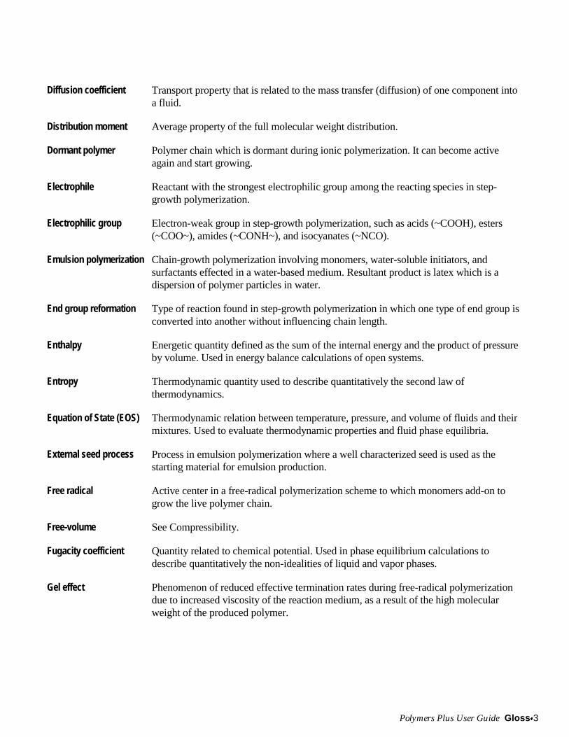
Polymers Plus User Guide Gloss x3
Diffusion coefficient Transport property that is related to the mass transfer (diffusion) of one component intoa fluid.
Distribution moment Average property of the full molecular weight distribution.
Dormant polymer Polymer chain which is dormant during ionic polymerization. It can become activeagain and start growing.
Electrophile Reactant with the strongest electrophilic group among the reacting species in step-growth polymerization.
Electrophilic group Electron-weak group in step-growth polymerization, such as acids (~COOH), esters(~COO~), amides (~CONH~), and isocyanates (~NCO).
Emulsion polymerization Chain-growth polymerization involving monomers, water-soluble initiators, andsurfactants effected in a water-based medium. Resultant product is latex which is adispersion of polymer particles in water.
End group reformation Type of reaction found in step-growth polymerization in which one type of end group isconverted into another without influencing chain length.
Enthalpy Energetic quantity defined as the sum of the internal energy and the product of pressureby volume. Used in energy balance calculations of open systems.
Entropy Thermodynamic quantity used to describe quantitatively the second law ofthermodynamics.
Equation of State (EOS) Thermodynamic relation between temperature, pressure, and volume of fluids and theirmixtures. Used to evaluate thermodynamic properties and fluid phase equilibria.
External seed process Process in emulsion polymerization where a well characterized seed is used as thestarting material for emulsion production.
Free radical Active center in a free-radical polymerization scheme to which monomers add-on togrow the live polymer chain.
Free-volume See Compressibility.
Fugacity coefficient Quantity related to chemical potential. Used in phase equilibrium calculations todescribe quantitatively the non-idealities of liquid and vapor phases.
Gel effect Phenomenon of reduced effective termination rates during free-radical polymerizationdue to increased viscosity of the reaction medium, as a result of the high molecularweight of the produced polymer.
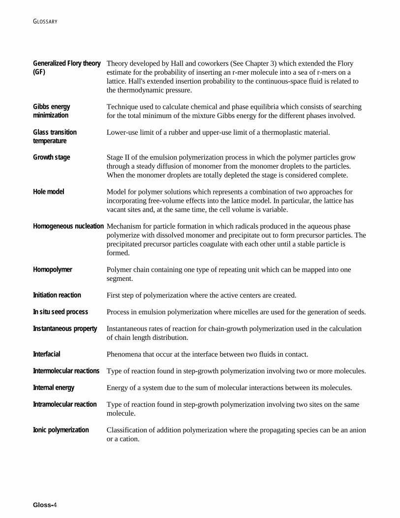
GLOSSARY
Gloss x4
Generalized Flory theory(GF)
Theory developed by Hall and coworkers (See Chapter 3) which extended the Floryestimate for the probability of inserting an r-mer molecule into a sea of r-mers on alattice. Hall's extended insertion probability to the continuous-space fluid is related tothe thermodynamic pressure.
Gibbs energyminimization
Technique used to calculate chemical and phase equilibria which consists of searchingfor the total minimum of the mixture Gibbs energy for the different phases involved.
Glass transitiontemperature
Lower-use limit of a rubber and upper-use limit of a thermoplastic material.
Growth stage Stage II of the emulsion polymerization process in which the polymer particles growthrough a steady diffusion of monomer from the monomer droplets to the particles.When the monomer droplets are totally depleted the stage is considered complete.
Hole model Model for polymer solutions which represents a combination of two approaches forincorporating free-volume effects into the lattice model. In particular, the lattice hasvacant sites and, at the same time, the cell volume is variable.
Homogeneous nucleation Mechanism for particle formation in which radicals produced in the aqueous phasepolymerize with dissolved monomer and precipitate out to form precursor particles. Theprecipitated precursor particles coagulate with each other until a stable particle isformed.
Homopolymer Polymer chain containing one type of repeating unit which can be mapped into onesegment.
Initiation reaction First step of polymerization where the active centers are created.
In situ seed process Process in emulsion polymerization where micelles are used for the generation of seeds.
Instantaneous property Instantaneous rates of reaction for chain-growth polymerization used in the calculationof chain length distribution.
Interfacial Phenomena that occur at the interface between two fluids in contact.
Intermolecular reactions Type of reaction found in step-growth polymerization involving two or more molecules.
Internal energy Energy of a system due to the sum of molecular interactions between its molecules.
Intramolecular reaction Type of reaction found in step-growth polymerization involving two sites on the samemolecule.
Ionic polymerization Classification of addition polymerization where the propagating species can be an anionor a cation.
Polymers Plus User Guide Gloss x5
Latex The final product obtained at the end of the emulsion polymerization after the seedstage, growth stage, and monomer finishing stage are complete.
Lattice model Model of polymer solutions based on the incompressible lattice theory which assumethat the lattice is occupied by both chains and vacant lattice sites or holes. Pure chainfluid is therefore treated as a binary mixture between molecules and holes.
Linear polymer Polymer with repeat units placed one after the other, without forming branches.
Liquid-liquid phaseequilibrium (LLE)
State of coexistence of two liquid phases at equilibrium.
Live polymer chain Term referring to growing polymer chains containing n segments, with an active centerattached to a segment of type i, i.e., segment formed from monomer i. Live polymer isrepresented using the symbol ( )Pn
i where the n refers to the chain length in terms of thenumber of segments or monomer units incorporated in the polymer chain.
Low molecular weightpolymer
Polymer formed from a high molecular weight polymer by random scission.
Lower critical solutiontemperature (LCST)
Temperature above which liquid-liquid phase split occurs in polymer mixtures due tofree volume effects.
Melt State of aggregation of a polymer at temperatures higher than its melting temperature.
Melting temperature Highest temperature at which polymer crystallites can exist.
Method of moments Method of calculating polymer properties through distribution moments or averages ofthe distribution rather than through the full distribution.
Micellar nucleation Mechanism for particle formation in which micelles act as the site of nucleation.
Micelles Aggregates of emulsifier molecules.
Monomers Small molecules. Two or more bond together form a polymer.
Monomer finishing stage Stage III of the emulsion polymerization process in which the reaction mixture consistsof the monomer swollen polymer particles and the aqueous medium. During this stagefurther polymerization of the monomer in the particles takes place and results in adecrease of the particle size due to the higher density of the polymer compared to themonomer.
Multimodal distribution Distribution which has several peaks in its graphical representation.
Nucleation period Time required for particle nucleation to be completed in emulsion polymerization, alsocalled nucleation time. Usually last 10-15 minutes in conventional polymerizationsystems.
GLOSSARY
Gloss x6
Nucleophile Reactant with the strongest nucleophilic group between the reacting species in step-growth polymerization.
Nucleophilic groups Electron-strong groups in step-growth polymerization, typically alcohols (~OH), amines(~NH2), or water.
Nucleophilic addition Bimolecular reaction mechanism in which electrophile and nucleophile combine toform a new functional group. These reactions are typically irreversible.
Nucleophilic substitution Bimolecular reaction mechanism in which reactions from a nucleophilic group from onereactant, nucleophile, displace a nucleophilic group in the other reactant, electrophile,resulting in two new products. These reactions tend to be highly reversible.
Oligomer Small polymer chain containing 20 or less repeating units. Structure and properties ofoligomers are fixed.
Perturbation Any deviation between the properties of the real and the reference fluid.
Perturbed-hard chaintheory (PHCT)
Theory developed by Prausnitz and co-workers (See Chapter 3) which represents thefirst attempt to combine the vast body of knowledge in statistical mechanics into apractical equation of state for industrial applications.
Phase equilibria Coexistence of two or more homogeneous phases at equilibrium.
Polydispersity Polymer property that accounts for the fact that a polymer is a multicomponent mixtureof species with differing chain lengths, chain compositions, and degrees of branching.The polydispersity represents the width of the full distribution of the polymer.
Polymer Macromolecule made up of many smaller repeating units providing linear and branchedchain structures.
Polymer fractionation Process during which the low molecular weight fractions of a polydisperse polymer areseparated from the high molecular weight fractions. This is often achieved by theaddition of an anti-solvent in the polymer solution, which tends to precipitate the highends of the polymer.
Precipitationpolymerization
Polymerization process where the formed polymer precipitates out of the reactionmedium.
Propagation reaction Main step of polymerization where monomers add-on to a growing polymer chain.
Polymers Plus User Guide Gloss x7
Pseudocondensationreaction
Type of reaction found in step-growth polymerization which involves rearrangement ofatoms in two different functional groups, resulting in a new functional group. No by-products are produced by pseudocondensation reactions. Pseudocondensation reactionscan involve two monomers, a monomer and a polymer end group, or two polymer endgroups, and are nucleophilic addition reactions.
Quasi-steady-stateapproximation (QSSA)
Assumption that live polymer moments attain their steady-state value instantaneouslyduring free-radical polymerization. This assumption makes the system of differentialequations much easier to integrate. QSSA is also referred to as stationary-statehypothesis.
Random scission reaction Type of reaction that occurs during polymerization which involves the spontaneouscleavage of a polymer chain due to thermal degradation.
Rearrangement reaction Type of reaction found in step-growth polymerization which occur between twopolymer molecules, resulting in two new polymer molecules with different molecularweights. These reactions may involve the end group of one molecule and an internal siteon another molecule, or they may involve internal sites on both molecules.
Reverse condensationreaction
Type of reaction found in step-growth polymerization where condensate moleculescleave an existing polymer chain, producing two smaller chains. Reverse condensationreactions near the end of a polymer molecule can generate free monomers
Ring-addition reaction Type of reaction found in step-growth polymerization which involves intermolecularreactions between polymer end groups and cyclic monomers or oligomers. The endgroup of the polymer links to the cyclic compound, opening the ring and lengthening thechain of the linear molecule.
Ring-opening reaction Type of reaction found in step-growth polymerization which involves intermolecularreactions between condensate or monomer molecules and cyclic monomers oroligomers. Condensate molecules or monomers react with cyclic compounds, openingthe ring structure to produce linear oligomers or cyclic monomers.
Ring-closing reaction Type of reaction found in step-growth polymerization which involves intramolecularreactions which occur between the two end groups of a linear molecule. Ring-closingreactions which occur between two end groups of a branched or network molecule arereferred to here as intramolecular cyclization to differentiate them from reactions whichform ring-shaped molecules.
Ring-scission reaction See Ring opening reactions.
Seed stage Stage I of the emulsion polymerization process in which particle nucleation iscompleted. Usually last 10-15 minutes in conventional polymerization systems.
Segments Repeating structure within a chain that is produced when monomers bond togetherthrough polymerization and become polymers.
GLOSSARY
Gloss x8
Semi-crystalline polymer Polymer which contains regions that are crystalline and regions that are amorphous. Thedegree of crystallinity determines the fraction of the polymer that is in crystalline form.
Single-site catalyst Catalyst with only one type of sites. These catalysts produce the same polymer on alltheir sites.
Solution polymerization Polymerization carried out in the presence of an inert solvent in which monomers andpolymers are dissolved.
Stationary statehypothesis
See Quasi-steady-state approximation.
Statistical associatingfluid theory (SAFT)
Theory developed by Gubbins, Radosz and collaborators (See Chapter 3) which uses areference fluid term to account for hard-sphere repulsions, chain formation, andchemical association or hydrogen-bonding.
Step-growthpolymerization
Classification of polymerization reactions in which monomers react with theirfunctional groups, resulting in a polymer chain that continues to grow from both ends aspolymerization progresses.
Surface tension Quantitative index of the tension of the surface layer of a liquid and its tendency tocontract to the smallest possible area.
Surface area Parameter that measures the surface area of chain molecules; used in some equations ofstate for chain molecules.
Suspensionpolymerization
Chain-growth polymerization involving monomers suspended as droplets in acontinuous phase (usually water) to which an oil-soluble initiator is added.
Tangent sphere model Model for polymer solutions which treats molecules as a chain of freely-jointed, tangenthard spheres, where segments on a chain are tangent with their neighboring segments,and can rotate freely without overlaps.
Terminal model Model which uses the assumption the rate of propagation is independent of the polymerchain length, and depends only on the concentration of monomers and active segmentson live polymer chains with active segments.
Terminal monomer loss Type of reaction found in step-growth polymerization involving the loss of a monomerunit at the end of a polymer chain due to thermal degradation mechanisms.
Termination reaction Last stage of polymerization where the active centers are destroyed and live polymerchains become dead polymer chains.
Thermal conductivity Transport property related to heat transfer.
Thermophysicalproperties
Volumetric and calorimetric properties of pure components and their mixtures.
Polymers Plus User Guide Gloss x9
Transport phenomena Transfer of mass, heat, and momentum at non-equilibrium conditions.
Unimodal distribution Distribution where the graphical representation mimics the normal bell-shaped curve.
Upper critical solutiontemperature (UCST)
Temperature below which liquid-liquid phase split occurs in polymer mixtures.
Vapor-liquid equilibrium(VLE)
State of coexistence of a liquid and a vapor phase at equilibrium.
Viscosity Transport property related to the rheological behavior of a fluid. It is a function of thepolymer size, the mixture composition, the temperature, and the shear rate.
Zero-shear viscosity Viscosity of a fluid at zero shear rate conditions.

GLOSSARY
Gloss x10
Polymers Plus User Guide Index x1
INDEX
This index includes entries in the Examples andApplications Case Book for your convenience.
AABS 3•43–3•44, 4•122Acrylonitrile-butadiene-styrene 3•43–3•44, 4•122Activation energy 3•56, 3•62, 4•99, 4•103, 4•138, 4•164, 4•182,
4•198, 5•81–5•82, G•2Activation volume 4•99, 4•103, 4•138Activity coefficient models
Flory-Huggins 3•12, 3•73–3•78NRTL 3•12, 3•79–3•87UNIFAC 3•13, 3•89–3•93UNIFAC free volume 3•13, 3•95–3•98
Addition polymers 2•43, 4•177Aggregate polymer 2•19, 2•21, 2•26, 2•30, 2•36, 2•38, 4•178,
4•186–4•187Amorphous solid 3•5Analysis tools 1•9, 5•103–5•109Arrhenius expression 3•56, 4•99, 4•103, 4•138–4•139, 4•164,
4•182Aspen Custom Modeler simulations
expandable polystyrene batch polymerization process DN•45–DN•52
LLDPE / HDPE process DN•25–DN•34polyethylene terephthalate continuous process DN•9–DN•18polyethylene terephthalate semi-batch/batch process DN•1–
DN•8polystyrene bulk polymerization process DN•19–DN•24polyvinyl chloride polymerization process DN•35–DN•44
Aspen Plus 1•7associating data with process streams 2•53data fit 5•77distillation models 5•16equilibrium reactor models 5•19ideal gas model 3•14, 3•99kinetic reactor models 5•20–5•56mass-balance reactor models 5•17–5•18property model calculations E•1property models 3•22PSRK EOS model 3•115pure component databank 2•11reactor models 5•16–5•17standard reaction models 4•8unit operation models 5•8–5•16, 5•85–5•92user kinetic models 5•92–5•96
Aspen Plus (continued)user physical property models 5•97–5•100
Attributescatalyst 2•32composite aggregate polymer 2•26composite live polymer 2•25composite polymer 2•23–2•24initialization scheme 2•20, 2•34–2•38site based aggregate polymer 2•30site based live polymer 2•29site based polymer 2•27user 2•33
Average properties 2•43, 2•45–2•46Azo-bis-isobutyronitrile SS•106
BBatch polymerization
expandable polystyrene DN•45–DN•52polyethylene terephthalate DN•1–DN•8
Benzene EX•77Beta-scission 4•107Binary parameters
interaction 3•76, 3•82, EX•41, EX•77Binary polymer solution viscosity 3•64, 3•67Branching
frequency 2•21, 2•24, 2•28, 4•167reactions 4•98, 4•106–4•107, 4•160–4•162, 4•167
Bulk distributionchain length moment equation 4•114
Bulk polymerization 4•6free-radical 4•95–4•120polystyrene DN•19–DN•24polystyrene by thermal initiation SS•1–SS•18
Butadiene SS•89
CCarnahan-Starling expression 3•127Case study block 5•106Catalysts
metallocene 4•153poisoning 4•167single site 4•153site activation 4•157, 4•164supported 4•153–4•156unsupported 4•153–4•156Ziegler-Natta 4•160–4•162
INDEX
Index x2
Categorizing polymers 2•5Cell models 3•106Chain
branching frequency 2•24, 2•28, 4•167initiation 4•102–4•104, 4•165scission 4•195, 4•196
Chain lengthaverage properties 2•46distribution 2•6, 2•20, 2•21, 2•23–2•27, 2•46–2•47, 2•50first moment 2•34, 4•112instantaneous weight distribution 2•49instanteous number-average 2•50second moment 4•112weight-average chain length 2•50zeroth moment 2•34, 4•112
Chain transferto agent 4•105, 4•161, 4•166, 4•185to hydrogen 4•160, 4•166to monomer 4•105, 4•160, 4•166, 4•180, 4•185to polymer 4•105, 4•112to solvent 4•105, 4•161, 4•166
Characterizingapproach 2•5components 1•10, 2•13
Class 0 component attributes 2•20, 2•33, 5•57Class 1 component attributes 2•20, 2•33Class 2 component attributes 2•20, 2•33–2•34, 5•31, 5•43, 5•57Closed-packed volume 3•109CMC 4•124Cocatalysts
poisoning 4•167Component attributes 2•6, 2•22–2•33
aggregate polymer 2•19, 2•21, 2•26, 2•30, 2•36, 2•38, 4•178,4•186–4•187
categories 2•21class 0 2•20, 2•33, 5•57class 1 2•20, 2•33class 2 2•20, 2•33–2•34, 5•31, 5•43, 5•57classes 2•20composite 2•21convergence 2•20degree of branching 2•19, 2•41degree of polymerization 2•9, 2•19, 2•44emulsion polymers 4•142for catalysts 2•20, 2•21, 2•32for ionic initiator 2•19, 2•21, 2•33for polymers 2•19, 2•21initialization 2•20, 2•34, 2•40live 2•19, 2•25, 2•29, 2•31, 2•36–2•37live polymer 2•21, 2•25, 2•29, 2•37molecular weight 2•9segment composition 2•9, 2•19site-based 2•27–2•30
Component attributes (continued)specifying 2•39–2•40specifying conventional 2•39specifying input language INPUT•5–INPUT•7specifying polymer 2•39specifying site-based 2•39structural properties tracked 2•9, 2•19tracking approach 2•19unit operation model treatment 5•57–5•59user-specified 2•33
Component databanksfor polymers 1•8, A•1–A•7for pure components 2•11, 3•92, A•1for segments 1•8, 2•11–2•12, A•1, A•8–A•49selecting 2•14
Componentscatalysts 2•10categories 2•7–2•10fortran utilities 5•87, H•1–H•32ionic initiators 2•8, 2•10property 2•11, 3•117site-based 2•10specifying 2•13–2•17specifying input language INPUT•2–INPUT•4types 2•14–2•15
Composite aggregate polymer set 2•22, 2•26Composite live polymer set 2•22, 2•25Composite polymer set 2•22–2•24Compressibility 3•13, 3•95, 3•106, 3•116Concentrated solution 3•64Condensation polymerization 4•2, 4•53Consumption of radicals 2•48–2•49, 4•103, 4•131Continuous process
polyethylene terephthalate DN•9–DN•18Conventional components 2•8, H•17
pure component constant values 3•118viscosity calculation 3•56
Convergencedata regression 5•79–5•83RBatch 5•52–5•56RCSTR 5•33–5•35RPlug 5•42–5•46
Coordination catalysts 4•152potential sites 4•164
Copolymerizationfree-radical 4•95–4•120ionic 4•175–4•192Ziegler-Natta 4•151–4•174
Critical concentrationpolymer solution 3•64
Critical micelle concentration 4•124Critical molecular weight 3•56Cross-linked polymers 2•9
Polymers Plus User Guide Index x3
Crystallinity parameter 3•23Cyclohexane SS•20
DData
collection 5•64, 5•65verification 5•64, 5•65
Data fitting 5•6, 5•61–5•83applications 5•62data collection 5•64, 5•65data verification 5•64, 5•65parameters 5•65–5•66steps for polymer models 5•63–5•68
Data regression 5•61–5•83convergence problems 5•79–5•83data collection 5•64, 5•65data verification 5•64, 5•65defining cases 5•76
fitting mixture parameters EX•41-EX•54flowsheet variables 5•70–5•71result interpretation 5•78sequencing cases 5•77standard deviation 5•75–5•76steps for polymer models 5•63–5•68steps for using tool 5•69
Databanksfunctional group 1•8polymer 1•8, A•1–A•7pure component 2•11, 3•92, A•1segment 1•8, A•8–A•49
Dead sites 2•20, 2•32, 4•166Defining
components 1•10feed streams 1•11polymerization kinetics 1•11
Degree ofbranching 2•19, 2•24, 2•28, 2•41polymerization 2•19–2•21, 2•23, 2•27, 2•44
Density function 2•45–2•46Density of copolymer 2•60, 2•62, 2•64Depolymerization 4•194, 4•195, 4•197Design specifications 5•105Devolatilization of monomers 3•6Diluent effect 3•67Distillation models 5•16Distribution
chain length moment equation 4•113–4•114displaying data for reactors 2•54–2•55displaying data for streams 2•55functions 2•43, 2•45–2•46moment equation 4•113–4•114moments 2•45–2•46, 4•108particle size 4•130, 4•139, 4•140–4•142
Distribution (continued)polymer 2•47, 2•51
Distribution calculationsselecting 2•54specifying 2•54–2•55
Di-tert-butyl peroxide SS•4Documentation 6•9Dodecyl mercaptan SS•4Dupl 5•9–5•11Dynamic models 1•7, 1•11
expandable polystyrene batch polymerization process DN•45–DN•52
LLDPE / HDPE process DN•25–DN•34polyethylene terephthalate continuous process DN•9–DN•18polyethylene terephthalate semi-batch/batch process DN•1–
DN•8polystyrene bulk polymerization process DN•19–DN•24polyvinyl chloride polymerization process DN•35–DN•44
Dynamic simulations 1•7
EEG DN•1, DN•9, DN•10Emulsion polymerization 4•121–4•149
accessing model 4•144applications 4•122attributes 4•142built-in reaction listing 4•145homogeneous nucleation 4•128–4•129kinetic scheme 4•123–4•139latex 4•125, 4•131micellar nucleation 4•124–4•127model features 4•139–4•141monomer partitioning 4•139–4•140particle growth 4•123, 4•130particle size distribution 4•130, 4•139, 4•140–4•142properties calculated 4•142radical balance 4•131–4•135rate constants 4•139seed process 4•130Smith-Ewart theory 4•135specifying calculation options 4•147specifying gel-effect 4•147specifying input language INPUT•30–INPUT•38specifying model 4•144specifying particle growth parameters 4•148specifying phase partitioning 4•148specifying rate constants 4•147specifying reacting species 4•145specifying reactions 4•146stage I (seed) 4•125, 4•140stage II (growth) 4•125, 4•130, 4•140stage III (finishing) 4•125styrene butadiene process SS•89–SS•103
INDEX
Index x4
End-use properties 2•59, 2•60–2•65adding a Prop-Set 2•66calculating 2•65, EX•91-EX•102selecting 2•65specifying input language INPUT•8–INPUT•10
Enthalpy 3•2–3•3condensation 3•24, 3•27formation 3•24, 3•27, 3•100–3•101, C•2ideal gas 3•100mixing 3•74, 3•80–3•82sublimation 3•24, 3•27
Entropy 3•3ideal gas 3•101mixing 3•74, 3•80–3•82
EPS DN•45– DN•52Equations of state
data regression EX•41-EX•54polymer SRK 3•115–3•122SAFT 3•123–3•134Sanchez-Lacombe 3•105–3•114
Equilibrium reactor models 5•7, 5•19REquil 5•19RGibbs 5•19
Estimationphysical properties 3•43physical property parameters 3•47–3•48solution viscosity 3•67
Ethanol EX•77Ethyl acetate
methyl methacrylate polymerization SS•125–SS•140Ethyl acrylate SS•105Ethyl benzene SS•4, SS•141Ethylene SS•19, SS•48Ethylene glycol DN•1, DN•9, DN•10Ethylene-polyethylene EX•41Ethylene-propylene 4•152, 4•155Excel
linking with Polymers Plus EX•24-EX•25Expandable polystyrene
batch polymerization process DN•45–DN•52Expansion coefficient 3•66
FFeed streams
conditions 2•34Flash2 5•11Flash3 5•11–5•12Flory-Huggins
activity coefficient model 3•12, 3•73–3•78, 3•95applicability 3•73concentration basis 3•76interaction parameter 3•17, 3•73, 3•82liquid-liquid equilibrium EX•77
Flory-Huggins (continued)parameters 3•77
Flowsheeting options 1•9, 5•104–5•106variables 5•106–5•108
Fluidized bed reactor 4•155Fortran
templates 6•3user models 6•4
Fortran utilitiescomponent attribute handling 5•88, H•3–H•16component handling H•17–H•25general stream handling H•26–H•31other H•32
Fractionating oligomers EX•77-EX•90Free energy 3•29–3•31Free volume calculations 3•97Free-radical polymerization 4•95–4•120
accessing model 4•115applications 4•96beta-scission reaction scheme 4•107built-in reaction listing 4•116bulk/solution 4•95–4•120chain transfer to small molecules 4•105equation for bulk polymer chain length 4•114equation for live chain length distribution 4•113equation for relationship between moments and properties
4•114gel effect 4•106, 4•109–4•111initiation reaction kinetic scheme 4•102–4•103kinetic scheme 4•97–4•107LDPE high pressure process SS•47–SS•64methyl methacrylate in ethyl acetate SS•125–SS•140model features 4•107–4•111phase equilibrium 4•109polystyrene SS•1–SS•18propagation reaction kinetic scheme 4•98, 4•104properties calculated 4•112–4•114quasi-steady state approximation 4•109rate expression 4•102, 4•103reaction kinetic scheme 4•97–4•107short/long chain branching reaction kinetic scheme 4•106–
4•107specifying calculation options 4•118specifying gel-effect 4•118specifying input language INPUT•22–INPUT•29specifying model 4•115specifying rate constants 4•118specifying reacting species 4•116specifying reactions 4•117styrene ethyl acrylate process SS•105–SS•124termination reaction kinetic scheme 4•105–4•106
Free-volume 3•95, 3•105–3•106Frequency function 2•45–2•46
Polymers Plus User Guide Index x5
FSplit 5•12Fugacity coefficient 3•2Functional group databank 1•8Functional groups
van Krevelen 3•43, C•1–C•11
GGas-phase polymerization 4•153
polypropylene process SS•155–SS•173Gel effect 4•106, 4•109–4•111, SS•109
correlation DN•38, DN•48Gel permeation chromatography 2•52Generalized Flory theory (GF) 3•107Generation of radicals 2•48, 4•131, 4•136–4•137Generic component attributes 2•33Gibbs free energy
excess 3•117liquid 3•29minimization 3•2, 3•10of condensation 3•30, 3•33of formation 3•30, 3•33, 3•101of mixing 3•74of sublimation 3•30, 3•33solid 3•32
Glass transition temperature 3•24, 3•27, 3•30, 3•33, 3•36, 3•39,C•3
correlation 3•41of mixture 3•69of pseudo-polymer 3•65of pseudo-solvent 3•66parameters 3•41polymer solution 3•69
Glycol DN•9GPC 2•52Group contribution method
predicting pure component properties EX•29-EX•40UNIFAC 3•89van Krevelen 3•10, 3•43
HHDPE
dynamic process DN•25–DN•34high temperature solution process SS•19–SS•46
Heat of polymerization 4•112Heater 5•12Hemoltz free energy 3•126High density polyethylene 4•152
dynamic process DN•25–DN•34high temperature solution process SS•19–SS•46
HIPP 4•155Hole models 3•106, 3•107Homosaturation solubility 4•140
Hydrogen SS•20
IIdeal gas
applicability 3•99departure functions 3•99enthalpy 3•100entropy 3•101parameter estimation 3•102parameters 3•102property model 3•99–3•103
Inhibition 4•106, 4•157–4•158, 4•160–4•162, 4•167catalyst sites 2•32, 4•158, 4•167
Initiationchain 4•102–4•104chemical 4•102decomposition 4•102, 4•131, 4•136, G•1–G•10free-radical polymerization 4•97, 4•102ionic 2•10, 2•21, 2•33, 4•179, 4•182radiation 4•103thermal 4•103, SS•1–SS•18
Input languagecatalysts INPUT•3–INPUT•4characterization inputs INPUT•3–INPUT•4components INPUT•2–INPUT•4emulsion INPUT•30–INPUT•38estimate INPUT•14free-rad INPUT•22–INPUT•29ionic INPUT•50–INPUT•57oligomers INPUT•3–INPUT•4polymers INPUT•3–INPUT•4properties INPUT•10–INPUT•14prop-set INPUT•8segment-bas INPUT•58–INPUT•59segments INPUT•3–INPUT•4step-growth INPUT•15–INPUT•21stream INPUT•5–INPUT•7Ziegler-Natta INPUT•38–INPUT•49
Installation 6•1–6•2Instantaneous number-average 2•50Instantaneous properties 2•45, 2•47–2•50Instantaneous weight chain length 2•49–2•50Interaction energy 3•109Intrinsic viscosity 2•63, 5•70, 5•83Ionic initiator 2•10, 2•33Ionic polymerization 4•175–4•192
accessing model 4•188applications 4•176built-in reaction listing 4•189kinetic scheme 4•178–4•185model features 4•186–4•187phase equilibria 4•186polymer properties calculated 4•187–4•188
INDEX
Index x6
Ionic polymerization (continued)propagation 4•180, 4•183properties calculated 4•187–4•188rate constants 4•182specifying input language INPUT•50–INPUT•57specifying model 4•188specifying rate constants 4•191specifying reaction species 4•189specifying reactions 4•190
KKinetics
emulsion polymerization 4•123–4•139fitting parameters EX•55-EX•76
free-radical polymerization 4•97–4•107ionic polymerization 4•178–4•185mechanisms 1•8melt polycarbonate 4•49–4•51multi-site models 2•52nylon reaction 4•37–4•48polyester reaction 4•30–4•36RBatch 5•46–5•56RCSTR 5•20–5•35reactor models 5•20–5•56reactors 2•51RPlug 5•35–5•46segment-based reaction model 4•198step-growth polymerization 4•25–4•51Ziegler-Natta polymerization 4•157–4•167
LLattice models 3•106Lattice theory 3•74, 3•106, 3•108LCST 3•8, 3•9, 3•105, 3•106, 3•112, 3•116LDPE SS•47–SS•64Linear condensation polymers 2•43Linear low density polyethylene 4•152
dynamic process DN•25–DN•34Liquid enthalpy
correlations 3•23parameters 3•24–3•25
Liquid Gibbs free energycorrelations 3•29parameters 3•30–3•31
Liquid molar volumecorrelations 3•35parameters 3•37
Liquid-liquid phase equilibrium (LLE) 3•8Live polymer 2•21, 2•25, 2•29, 2•37, 4•187
chain length distribution moment equation 4•113LLDPE
dynamic process DN•25–DN•34
Long chain branching 2•23, 2•27, 2•60, 4•112, 4•167, 4•169Loop reactors 4•154, 4•155Low density polyethylene 4•96
high pressure process SS•47–SS•64Low molecular weight polymer 2•43Lower critical solution temperature 3•8, 3•9, 3•105, 3•106, 3•112,
3•116
MMark-Houwink equation 3•56Mass-balance reactor models 5•17–5•18
RStoic 5•17RYield 5•18
Mass-based property parameters E•1–E•2Material streams 2•34Melt index 1•5, 2•60–2•61, 2•64–2•65, 5•70Melt index ratio 2•60, 2•65Melt polycarbonate
reaction kinetics 4•49–4•51Melt transition temperature 3•24, 3•27, 3•30, 3•33, C•3
correlation 3•21, 3•42parameters 3•42
Metallocene based catalysts 4•153Methanol EX•55Method of instantaneous properties 2•6, 2•45, 2•47–2•50, 2•51Method of moments 2•45, 2•47, 4•108, 4•168, 4•186Methyl methacrylate
polymerization in ethyl acetate SS•125–SS•140Methyl peroxide EX•55Mixer 5•13Mixing 1•9, 3•65–3•66Model parameters
fitting 5•65–5•66Models
adding in-line Fortran 5•105application tools 5•103–5•109case studies 5•106design specifications 5•105equations of state (EOS) 3•105–3•134optimization 5•106possible uses 5•103preliminary development 5•67refining 5•68sensitivity study 5•105steady-state unit operation 5•7–5•60trend analysis 5•67unit operation 1•9user unit operation calculations 5•86–5•91user unit operation model structure 5•86
Modified Mark-Houwink equation 3•56Molecular weight 1•5, 1•7, 2•11, 2•23, 2•29
control of 4•105critical 3•56
Polymers Plus User Guide Index x7
Molecular weight (continued)number-average 2•27, 2•64weight-average 2•21, 2•23, 2•27, 2•63, 2•64, 3•56
Moments of chain length distributionfirst 2•23, 2•24–2•25, 2•27, 2•34, 4•113, 4•114second 2•23, 2•27, 4•113, 4•114third 2•23, 2•27, 4•113, 4•114zeroth 4•113, 4•114
Moments of particle size distribution 4•140–4•141Monomers 2•2, 2•8
devolatilization of 3•6partitioning 4•139–4•140synthesis 1•2–1•5, 5•3, 5•4
Most-probable distribution 2•44, 4•36, 4•40, 4•46–4•47, 4•59Mult 5•14
Nn-butyl-acrylate EX•29NRTL
activity coefficient model 3•79–3•87applicability 3•79comparison of models 3•79, 3•86interaction parameters 3•81, 3•84parameters 3•85polymer model 3•80–3•82random copolymer model 3•83–3•84
Nucleationhomogeneous 4•128–4•129micellar 4•124–4•127
Nucleophilic reactions 4•25definitions 4•27
Number-averagedegree of polymerization 2•21, 2•23molecular weight 2•23, 2•27
Nylon 4•19–4•23caprolactam polymerization process SS•65–SS•87reaction kinetics 4•37–4•48user-specified reactions 4•40, 4•46
OOccupied sites 2•32Oligomers 2•2, 2•5, 2•9, 2•11, 3•5
fractionating EX•77-EX•90specifying 2•16
Optimization 5•106Organoaluminum catalysts 4•153, 4•164
PParameters
estimation 3•43glass transition 3•41liquid enthalpy 3•24–3•25
Parameters (continued)liquid Gibbs 3•30–3•31liquid molar volume 3•37melt transition 3•42NRTL models 3•85polymer SRK EOS 3•119SAFT EOS 3•132solid enthalpy 3•27–3•28solid Gibbs 3•33–3•34solid molar volume 3•39–3•40Tait model 3•53van Krevelen estimation 3•43
Perturbation theory 3•125Perturbed hard-sphere theory 3•127Perturbed-hard chain theory 3•107PET (see polyethylene terephthalate)Phase equilibria
ionic polymerization 4•186modeling 3•6step-growth polymerization 4•52Ziegler-Natta polymerization 4•168
PHCT 3•107, 3•127Physical properties
customized 3•45enthalpy 3•2–3•3entropy 3•3estimation 3•43estimation method 3•47–3•48fitting parameters 5•65–5•66Flory-Huggins 3•77fugacity coefficient 3•2ideal gas 3•102input language INPUT•10–INPUT•14liquid Gibbs free energy 3•29–3•31mass-based E•1–E•2modified Mark-Houwink viscosity 3•58NRTL 3•13, 3•85POLYSRK EOS 3•119POLYUFV 3•95
predicting parameters EX•29-EX•40Sanchez-Lacombe EOS 3•112solid Gibbs free energy 3•32solution viscosity 3•67specifying 3•44–3•49Tait 3•53UNIFAC 3•92UNIFAC free volume 3•97van Krevelen 3•63
Physical property parametersentering data 3•46–3•49optimization 3•49
Pipe 5•15Plant data fitting 5•61–5•83
INDEX
Index x8
Plasticizer effect 3•69Plug flow reactor 2•47, 2•51, 4•70PMMA SS•125–SS•140Poly(butyl-acrylate) EX•29Polycarbonate 4•23–4•24Polydispersity 3•4
index 2•23, 2•43, 2•50Polyester 4•12–4•18
reaction kinetics 4•30–4•36technology package 4•18
Polyethylene SS•19–SS•46, DN•25product EX•91
Polyethylene terephthalatebatch step-growth polymerization 4•16–4•17continuous process DN•9–DN•18continuous step-growth polymerization 4•12–4•15semi-batch/batch process DN•1–DN•8user-specified reactions 4•36
Polyisobutylene 4•5, 4•193, 4•196POLYMER databank 1•8, 2•12, A•1–A•7Polymer NRTL 3•79–3•87Polymerization 1•2–1•6
degree of 2•9, 2•19–2•21, 2•23, 2•27, 2•44emulsion 4•6, 4•121–4•149free-radical 4•95–4•120heat of 4•112ionic 4•175–4•192step-growth 4•11–4•94suspension DN•35Ziegler-Natta 4•151–4•174
Polymers 2•2, 2•9addition 2•43, 4•177aggregate 2•19, 2•21, 2•26, 2•30, 2•36, 2•38, 4•178, 4•186–
4•187attributes 1•7, 1•11, 4•112, 4•169branched 2•2, 2•9by property 2•4characterizing 2•5component characterization 1•7data fitting models 5•63–5•68dead 2•21, 4•98–4•105, 4•159definition 1•2distribution 2•50, 2•53, 4•58fractionation 3•10linear condensation 2•43live 2•21, 2•25, 2•29, 2•37, 4•187low molecular weight 2•43mass 2•51, 4•199method of instantaneous properties 2•6, 2•45, 2•47, 2•51method of moments 2•45, 2•47, 4•108, 4•168, 4•186monomer synthesis 1•2–1•5, 5•3, 5•4nomenclature for A•3–A•7processing 1•2–1•6, 5•2–5•5
Polymers (continued)production of molecules 2•49properties 2•5, 2•6, 2•59, 4•112–4•114, 4•169, 4•187–4•188property parameters A•2purification 1•2–1•5recovery 1•2–1•4, 1•6, 5•3, 5•4segments 1•10, 2•10, 3•80, 3•92, 4•57, A•8–A•49separation 1•2–1•4, 1•6, 5•3, 5•4solution viscosity 3•14, 3•55, 3•64, 3•67specifying 2•15–2•16structure 2•5synthesis 5•4tracking properties of 1•1, 2•19types 2•2viscosity models 3•55–3•71
Polymers Pluscalculating end-use properties EX•91-EX•102
configuration tips 6•3creating a simulation model EX•1-EX•28data regression EX•41–EX•54
features 1•1, 1•7–1•11, 5•103–5•109, 6•1fitting kinetic parameters EX•55–EX•76fractionating oligomers EX•77–EX•90
installation 6•1–6•2linking with Excel EX•24–EX•25predicting physical properties EX•29–EX•40
troubleshooting 6•4–6•8user fortran models 6•3–6•4
Polymethyl methacrylate 4•193, SS•125–SS•140Polyolefin EX•91, SS•47
production EX•41Polypropylene 4•5, 4•107, 4•152, 4•154
gas-phase polymerization processes SS•155–SS•173POLYSAFT
model parameters 3•132SAFT EOS model 3•123–3•134
POLYSRKmodel parameters 3•119polymer SRK EOS model 3•115–3•122
Polystyrene EX•29, EX•77, DN•45bulk polymerization by thermal initiation SS•1–SS•18dynamic bulk polymerization process DN•19–DN•24styrene monomer distillation SS•141–SS•154
Polyvinyl acetate 4•194, 4•196Polyvinyl chloride
dynamic polymerization process DN•35–DN•44Population balance method 4•108, 4•168Potential sites 2•20, 2•32, 4•164Process feed streams 1•11, 2•9, 2•20, 2•34Process modeling 1•4–1•6, 3•1–3•16
data fitting 5•63–5•68dynamic 1•7, 1•11, DN•1–DN•52flowsheets 5•5
Polymers Plus User Guide Index x9
Process modeling (continued)steady-state 1•7, 1•11, 4•18, 5•1–5•60, SS•1–SS•173steady-state features 5•5–5•6
Production rate of polymer 2•49Propagation 4•98, 4•104, 4•160–4•162, 4•165, 4•180, 4•183
rate 2•48Property distributions 2•41, 2•43, 2•44, 2•47
bimodal 2•42, 2•45bivariate 2•42multimodal 2•42unimodal 2•42
Property methods 1•8, 3•15–3•16customized 3•45POLYFH B•1–B•3POLYNRTL B•4–B•5, SS•4, SS•70, SS•93, SS•144, SS•159,
DN•12, DN•22, DN•28, DN•37, DN•47POLYSAFT 3•123, B•14–B•15, F•1POLYSL B•10–B•11, F•1, SS•50POLYSRK B•12–B•13POLYUF B•6–B•7POLYUFV B•8–B•9selecting 3•44–3•45
Property parameter databanks 1•8Prop-Set 2•62, 4•52, 5•70, 5•74, 5•83, Ex•91Pseudo-components
approach EX•77Pseudocondensation reactions 4•27Pseudo-polymer 3•64–3•66, 3•70Pseudo-solvent 3•64–3•66Pump 5•15Pure components
databank 2•11, 3•92, A•1predicting properties for polymers EX•29-EX•40
Purification 1•2–1•5PVC DN•35–DN•44
QQSSA 2•21, 4•109, 4•132Quackenbos 2•64–2•65Quasi-binary system 3•64, 3•70
RRadFrac 5•16Rate constant parameters 4•74, 4•164, 4•167, 4•182
data-fitting 5•6initiator decomposition G•1–G•10
Rate expressionfree-radical 4•53, 4•102, 4•103ionic 4•182segment-based reactions 4•198step-growth 4•61, 4•62, 4•63, 4•68, 4•74Ziegler-Natta 4•164
RBatch 5•46–5•56RCSTR 5•20–5•35Reaction models
Aspen Plus 5•7–5•60Reaction order 4•164Reactions
combination 4•197user-specified step-growth 4•67–4•68
Reactor models 5•16–5•17Recovery/separation 1•2–1•4, 1•6, 5•4REquil 5•19Reverse condensation reactions 4•27RGibbs 5•19RPlug 5•35–5•46RStoic 5•17Run procedures
for Polymers Plus 6•1–6•3RYield 5•18
SSAFT 3•13, 3•107SAFT EOS model 3•123–3•134
applicability 3•123fluid mixtures 3•128–3•130fluid system application 3•130–3•132
Sanchez-Lacombe EX•41applicability of EOS models 3•105EOS models 3•105–3•114parameters 3•112
SBR SS•89Schulz-Flory distribution 2•44Scission 4•28, 4•196Seed process 4•130Segment approach 2•13, 3•79, 3•83, 3•86Segment composition 2•2, 2•10, 2•19SEGMENT databank 1•8, 2•11–2•12, A•1, A•8–A•49Segment-based reaction model 4•193–4•203
accessing model 4•200applications 4•193assumptions 4•199backbone modifications 4•196chain scission 4•196combination reactions 4•197depolymerization 4•197kinetics 4•198properties calculated 4•199rate expression 4•198reaction categories 4•195–4•198reactions allowed 4•195–4•198side group modifications 4•196specifying input language INPUT•58–INPUT•59specifying model 4•200specifying rate constants 4•202
INDEX
Index x10
Segment-based reaction model (continued)specifying reaction scheme 4•201specifying reaction settings 4•201specifying reactions 4•202
Segments 2•10, 2•12, 2•13closed-packed volume 3•109mole flow 2•23mole fraction 2•23nomenclature for A•9–A•49property parameters A•8specifying 2•15structure 2•2types 2•10
Semi-batch polymerizationpolyethylene terephthalate DN•1–DN•8
Semi-crystalline copolymer density 2•64Semi-crystalline solid 3•5Sensitivity blocks 5•105Sep 5•15Sep2 5•15Separation/recovery 1•2–1•4, 1•6, 5•4Short chain branching frequency 2•24, 2•28Simulations
application tools 5•103–5•109creating a model EX•1-EX•28
templates 6•3Site activation 4•160–4•162, 4•164Site deactivation 4•166–4•167Site inhibition 4•158, 4•160–4•162, 4•167Site-based aggregate polymer set 2•22, 2•30Site-based components
attributes 2•27–2•30specifying 2•17
Site-based live polymer set 2•22, 2•29Site-based polymer set 2•22, 2•27–2•28Site-based species attributes 2•32–2•33Slurry processes 4•153–4•156Smith-Ewart theory 4•135Solid enthalpy
correlations 3•26parameters 3•27–3•28
Solid Gibbs free energycorrelations 3•32parameters 3•33–3•34
Solid molar volumecorrelations 3•38parameters 3•39–3•40
Solution polymerization 4•97, 4•153Solution viscosity
estimation 3•67–3•68parameters 3•67
Specifyingadditional simulation options 1•11component attributes 2•39–2•40components 2•13–2•17databanks 2•14distribution calculations 2•54–2•55emulsion kinetics 4•144end-use properties 2•65–2•66free-radical kinetics 4•115–4•118global simulation options 1•10ionic kinetics 4•188–4•191physical properties 3•44–3•49property methods 3•44–3•45property models 1•11segment-based reactions 4•200–4•202step-growth kinetics 4•87–4•93UOS model operating conditions 1•11Ziegler-Natta polymerization 4•170–4•173
Standard conventional components 2•8Standard deviation
entering in data regession 5•75–5•76Star copolymer 2•2Stationary state hypothesis 4•132Steady-state models
HDPE high temperature solution process SS•19–SS•46LDPE high pressure process SS•47–SS•64methyl methacrylate polymerization in ethyl acetate SS•125–
SS•140nylon 6 caprolactam polymerization processSS•65–SS•87polypropylene gas-phase polymerization processes SS•155–
SS•173polystyrene bulk polymerization by thermal initiation SS•1–
SS•18polystyrene with styrene monomer distillation SS•141–SS•154styrene butadiene emulsion copolymerization process SS•89–
SS•103styrene ethyl acrylate free-radical copolymerization process
SS•105–SS•124Steady-state unit operation models 5•7–5•60
distillation 5•16equilibrium reactor 5•19kinetic reactor 5•20–5•56mass-balance reactor 5•17–5•18reactor 5•16–5•17
Step-growth polymerization 4•11–4•94accessing model 4•87applications 4•12batch PET 4•16–4•17built-in reaction listing 4•89continuous PET 4•12–4•15functional groups 4•4, 4•25, 4•54, 4•57kinetic scheme 4•25–4•51melt polycarbonate reaction kinetics 4•49–4•51
Polymers Plus User Guide Index x11
Step-growth polymerization (continued)model features 4•11, 4•52–4•53model predictions 4•52model structure 4•53–4•87model-generated reactions 4•61–4•66nucleophilic reactions 4•25nylon 4•19–4•23, 4•37–4•48nylon 6 caprolactam polymerization process SS•65–SS•87phase equilibria 4•52polycarbonate 4•23–4•24polyester 4•12–4•18, 4•30–4•36polyester technology package 4•18rate constants 4•31, 4•37, 4•42, 4•48, 4•49, 4•61rate expression 4•61, 4•62, 4•63, 4•68, 4•74reacting species 4•57–4•58reaction stoichiometry 4•60specifying components 4•89specifying input language INPUT•15–INPUT•21specifying model 4•88specifying rate constants 4•90, 4•92specifying report options 4•92specifying subroutines 4•93user reactions 4•91–4•92user subroutines 4•69–4•87
Stirred bed reactors 4•154–4•156Stockmayer 2•43, 2•44Structure
of monomers 2•2, 2•8of oligomers 2•2, 2•5, 2•9, 2•11, 2•13of polymers 2•2–2•5, 2•9of segments 2•2, 2•10, 2•13
Styrene EX•30, SS•1, SS•89, SS•105, SS•141, DN•19monomer distillation of polystyrene SS•141–SS•154
Styrene butadieneemulsion copolymerization process SS•89–SS•103
Styrene-butadiene rubber SS•89Styrene-butyl-acrylate EX•30Styrene ethyl acrylate
free-radical copolymerization process SS•105–SS•124Surface area 3•107Suspension polymerization DN•35
TTait molar volume model 3•51–3•54
applicability 3•51coefficients D•1–D•2equation 3•52, 3•97parameters 3•53
Tangent-sphere models 3•107Temperature
glass transition 3•24, 3•27, 3•30, 3•33, 3•36, 3•39, C•3glass transition estimation 3•41melt transition estimation 3•42
Templatesfortran 6•3polymer simulation 6•3
Terephthalic acid DN•9Terminal double bond polymerization 4•157Termination models 4•98, 4•159Thermal initiation
polystyrene bulk polymerization SS•1–SS•18Tips
configuration 6•3TPA DN•9Troubleshooting 6•4–6•8True solvent dilution effect 3•67, 3•70Two dimensionless parameters 2•48
UUCST 3•8, 3•9, 3•13, 3•106, 3•112UNIFAC
activity coefficient model 3•13, 3•89–3•93applicability 3•89functional groups 3•90–3•91parameters 3•92physical property method B•6–B•7
UNIFAC free volumeactivity coefficient model 3•95–3•98applicability 3•95parameters 3•97physical property method B•8–B•9
Unit operation models 1•9, 5•8–5•16Aspen Plus 5•7–5•60calculations for user models 5•86–5•91component attribute treatment 5•57–5•59Dupl 5•9–5•11Flash2 5•11Flash3 5•11–5•12FSplit 5•12Heater 5•12Mixer 5•13Mult 5•14Pipe 5•15Pump 5•15RadFrac 5•16Sep 5•15Sep2 5•15structure for user models 5•86user 5•85–5•102
Upper critical solution temperature 3•8, 3•9, 3•13, 3•106, 3•112User attributes 2•33User component attributes 2•33User models 5•85–5•102
calculations 5•86–5•91development 5•97–5•100kinetic 5•92–5•96
INDEX
Index x12
User models (continued)physical property 5•97–5•100structure 5•86unit operation 5•85–5•92
User properties 4•167User reactions
nylon 4•40nylon salt 4•46polyethylene terephthalate 4•36rate expression 4•68step-growth polymerization 4•67–4•68
User subroutinesstep-growth polymerization 4•69–4•87
VVacant sites 2•32, 4•158Van der Waals 3•129
volume 3•36, 3•39, C•2Van Krevelen
functional groups 3•62, C•1–C•11group contribution EX•29-EX•40
liquid Gibbs free energy 3•29–3•31liquid molar volume 3•35–3•37models 3•21–3•50solid Gibbs free energy 3•32–3•34solid molar volume 3•38–3•40thermophysical property models 3•21–3•50viscosity-temperature relationship 3•69
Van Krevelen models 3•21, 3•22, 3•43applicability 3•21glass transition temperature correlation 3•41group contribution 3•43, EX•29–EX•40input language INPUT•10–INPUT•14liquid enthalpy 3•23–3•25melt transition temperature estimation 3•21, 3•42parameter estimation 3•43parameters 3•63solid enthalpy 3•26–3•28
Vapor-liquid equilibrium (VLE) 3•6Vinyl acetate EX•55Viscosity
binary solution estimation 3•67concentrated polymer solutions 3•64–3•70critical mass 3•56, 3•59, 3•62dilution effect 3•67estimation 3•67mixture 3•66, 3•67, 3•70models 3•55–3•71polymer melt 3•56, 3•62, 3•69polymer solution 3•14, 3•64, 3•67temperature correlation 3•59–3•63zero-shear 2•63, 3•14, 3•55–3•56, 3•59, 3•65
Volumeactivation 4•99, 4•103, 4•138closed-packed 3•109expansion coefficient 3•66
WWeight-average
degree of polymerization 2•9, 2•19, 2•25, 2•26, 2•27, 2•29,2•30, 2•44
molecular weight 2•23Williams-Landel-Ferry 3•59
ZZero-shear viscosity 2•63, 3•14, 3•55–3•56, 3•59, 3•65Ziegler-Natta catalysts 2•10, 4•160–4•162
attributes 2•32dead sites 2•20, 2•32inhibited sites 2•32occupied sites 2•32potential sites 2•20, 2•32vacant sites 2•32
Ziegler-Natta polymerization 4•151–4•174accessing model 4•170applications 4•152built-in reaction listing 4•171bulk process 4•155, 4•156catalyst site activation 4•164catalyst states 4•157–4•158chain initiation 4•165chain transfer to small molecules 4•166dynamic modeling of LLDPE / HDPE DN•25–DN•34gas-phase process 4•155, 4•156HDPE high temperature solution process SS•19–SS•46inhibition reaction scheme 4•157–4•162, 4•167internal double-bond polymerization 4•159kinetic scheme 4•157–4•167long chain branching reaction scheme 4•167model features 4•168phase equilibria 4•168poisoning reaction scheme 4•167polyethylene processes 4•154polymer properties calculated 4•169polypropylene gas-phase polymerization processes SS•155–
SS•173propagation reaction scheme 4•160–4•162properties calculated 4•169propylene process 4•154–4•156rate constants 4•164rate expression 4•164site deactivation 4•166–4•167slurry process 4•153–4•156solution process 4•153

Polymers Plus User Guide Index x13
Ziegler-Natta polymerization (continued)specifying input language INPUT•38–INPUT•49specifying model 4•170specifying rate constants 4•173specifying reacting species 4•171specifying reactions 4•172terminal double bond 4•157

INDEX
Index x14
COMMENTS
Name
Title
Company
Address
Telephone
What did you like most about this User Guide?
What did you like least about this User Guide?

What improvements or changes would you like in this User Guide?
What specific topics would you like included in this User Guide?
If you found any errors in this User Guide, list the error and page number:
Additional comments:
Forward this form to:
Aspen Technology, Inc.Attn: Polymer Technology CoordinatorTen Canal ParkCambridge, Massachusetts 02141USATelefax: +1-617/949-1030


![ss{]a-dn -Xew ersion for the intelectually... · 6 _p≤n-]-c-amb sh√p-hnfn t\cn-Sp-∂- Ip´nIfpsS hnZym`ymkw $ ]mTy]≤Xn ersion Abbreviations Used RTE Act - Right To Education](https://img.pdfslide.tips/doc/110x75/5e8d91cb537c9a444572d3ed/ssa-dn-xew-for-the-intelectually-6-pan-c-amb-shap-hnfn-tcn-sp-a-.jpg)

![Thermochemistry [ Enthalpy and Calorimetry]](https://img.pdfslide.tips/doc/110x75/557ddce9d8b42a4e358b4993/thermochemistry-enthalpy-and-calorimetry.jpg)