Estimating mixed layer nitrate in the North Atlantic Ocean · 1Leibniz Institut fur Meereswissenschaften (IFM-GEOMAR), Kiel, Germany¨ 2International Paciﬁc Research Center, School

Biogeosciences, 7, 795–807, 2010www.biogeosciences.net/7/795/2010/© Author(s) 2010. This work is distributed underthe Creative Commons Attribution 3.0 License.

Biogeosciences

Estimating mixed layer nitrate in the North Atlantic Ocean

T. Steinhoff1, T. Friedrich 2, S. E. Hartman3, A. Oschlies1, D. W. R. Wallace1, and A. Kortzinger1

1Leibniz Institut fur Meereswissenschaften (IFM-GEOMAR), Kiel, Germany2International Pacific Research Center, School of Ocean and Earth Science and Technology, University of Hawaii at Manoa,Honolulu, Hawaii, USA3National Oceanography Centre, Southampton, UK

Received: 29 July 2009 – Published in Biogeosciences Discuss.: 3 September 2009Revised: 27 January 2010 – Accepted: 23 February 2010 – Published: 1 March 2010

Abstract. Here we present an equation for the estimation ofnitrate in surface waters of the North Atlantic Ocean (40◦ Nto 52◦ N, 10◦ W to 60◦ W). The equation was derived bymultiple linear regression (MLR) from nitrate, sea surfacetemperature (SST) observational data and model mixed layerdepth (MLD) data. The observational data were taken frommerchant vessels that have crossed the North Atlantic on aregular basis in 2002/2003 and from 2005 to the present. Itis important to find a robust and realistic estimate of MLDbecause the deepening of the mixed layer is crucial for ni-trate supply to the surface. We compared model data fromtwo models (FOAM and Mercator) with MLD derived fromfloat data (using various criteria). The Mercator model givesa MLD estimate that is close to the MLD derived from floats.MLR was established using SST, MLD from Mercator, timeand latitude as predictors. Additionally a neural network wastrained with the same dataset and the results were validatedagainst both model data as a “ground truth” and an indepen-dent observational dataset. This validation produced RMSerrors of the same order for MLR and the neural network ap-proach. We conclude that it is possible to estimate nitrateconcentrations with an uncertainty of±1.4 µmol L−1 in theNorth Atlantic.

1 Introduction

Estimating seasonal new production is fundamental for ourunderstanding of the global carbon cycle. Especially in re-gions where nitrate is depleted during summer the amount ofnitrate that is available at the onset of the productive season

Correspondence to:T. Steinhoff([email protected])

is essential for further production estimates estimates. Inter-annual changes of the nitrate availability will directly influ-ence new production and carbon drawdown (Koeve, 2001).But estimating nutrient fluxes into the upper ocean and theirsubsequent utilisation by marine primary production is still abig challenge in oceanography. Even though there are con-tinuous sampling programs at Bermuda Atlantic Time Series(BATS, Bates, 2007) station in the western North Atlanticand European Station for Time Series in the Ocean, CanaryIslands (ESTOC,Gonzalez-Davila et al., 2007) in the easternpart of the subtropical North Atlantic, it is impossible to mapnutrient variability for the whole basin. The mechanism ofnutrient supply is very different at the two stations: at BATSit is mainly driven by eddies and at ESTOC by winter con-vection (Cianca et al., 2007). Furthermore these two stationsare located in the subtropical gyre where seasonality is low.In the temperate North Atlantic, between 30◦ N and 60◦ N,the coverage of surface nutrient data is sparse especially be-cause of very few wintertime observations.Kortzinger et al.(2008) andHartman et al.(2010) reported the seasonal cycleof nutrient data for the years 2003/2004 with data from a sin-gle location, the Porcupine Abyssal Plain site (PAP), locatedin the temperate North East Atlantic Ocean (49◦ N, 16.5◦ W).

Some work has been done to estimate winter nitrateconcentrations from nitrate-density relationships (Garsideand Garside, 1995), nitrate-temperature/density relationships(Kamykowski and Zentara, 1986; Sherlock et al., 2007) orto estimate nutrient fields from remotely sensed data (Goeset al., 2000; Kamykowski et al., 2002; Switzer et al., 2003).Several other attempts were made to estimate wintertime ni-trate concentration (e.g.Takahashi et al., 1985; Glover andBrewer, 1988; Kortzinger et al., 2001; Koeve, 2001) as thevalues at the onset of the productive season are crucial to as-sess new production (Minas and Codespoti, 1993).

Published by Copernicus Publications on behalf of the European Geosciences Union.

http://creativecommons.org/licenses/by/3.0/

796 T. Steinhoff et al.: Estimating nitrate in the North Atlantic

Another possible application of predicting seasonal nutri-ent cycles, that are not based on climatology, is the parame-terization of CO2 partial pressure in seawater (pCO2). Stud-ies have been performed to relate thepCO2 in the North At-lantic to remotely sensed data (Lefevre et al., 2005; Jametet al., 2007; Luger et al., 2008; Chierici et al., 2009; Friedrichand Oschlies, 2009a,b; Telszewski et al., 2009) as it is drivenby many factors: thermodynamics, biology, mixing and air-sea gas exchange. Chlorophylla (chl-a) concentrations areoften employed to estimate the biological driver of thepCO2,but the utility of chl-a for this purpose is rather limited (Onoet al., 2004; Luger et al., 2008). Given that nitrate changesare directly related to new production we believe that estima-tion of the entire seasonal cycle of nitrate could also improvepCO2 predictions.

Here we present (and compare) two methods using obser-vational data to estimate mixed-layer nitrate in the North At-lantic between 40◦ N and 52◦ N and 10◦ W and 60◦ W. Thefirst method is a multi linear regression (MLR) and the sec-ond method used the same data to train a neural network.

However, the quality of any prediction depends on thequality of the predictors. Therefore we chose the variables tobe used in the prediction, sea surface temperature (SST) andMLD, very carefully. Reliable and well tested SST prod-ucts are available (e.g. the Advanced Microwave ScanningRadiometer-EOS (AMSR-E) on NASA EOS Aqua satellite,Emery et al., 2006). The situation is more complicated forMLD because there is no uniform criterion for its estimation.Numerous criteria for the estimation of MLD can be foundin the literature (e.g.Kara et al., 2003; de Boyer Montegutet al., 2004) and often the criteria need to be adjusted re-gionally. The proposed criteria vary from simple temper-ature difference criteria to advanced methods such as thecurvature criterion ofLorbacher et al.(2006) that uses theshape of vertical profiles (temperature or density). For allthese criteria temperature/density profiles are required forthe MLD estimation. Alternatively, MLD climatologies orMLD estimates from models can be used. In this study wecompare MLD calculated from in-situ measured profiles (i.e.by ARGO floats), MLD climatology ofMonterey and Lev-itus (1997), and MLD estimates from two different models(FOAM and Mercator).

2 Data and calculations

2.1 Discrete water samples

We used data from water samples taken on “Volunteer Ob-serving Ships” (VOS) along a trans-Atlantic route betweenEurope and North America (Fig.1a). The studies werepart of two European research projects: CArbon VAriabilityStudies by Ships Of Opportunity (CAVASSOO) and CAR-BOOCEAN. During CAVASSOO (2002/2003) samples werecollected from the merchant vessel M/V Falstaff (Wallenius

60 oW 48 oW 36 oW 24 oW 12 oW

30 oN

36 oN

42 oN

48 oN

54 oN

60 oN

BATS40°N/49°W

ESTOC

PAP

60 oW 48 oW 36 oW 24 oW 12 oW

30 oN

36 oN

42 oN

48 oN

54 oN

60 oN

6

5

4

3

2

1

aa

bb

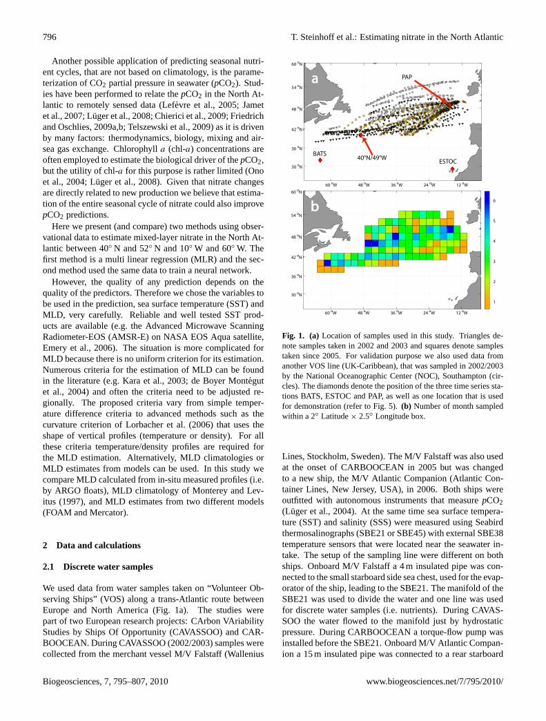
Fig. 1. (a) Location of samples used in this study. Triangles de-note samples taken in 2002 and 2003 and squares denote samplestaken since 2005. For validation purpose we also used data fromanother VOS line (UK-Caribbean), that was sampled in 2002/2003by the National Oceanographic Center (NOC), Southampton (cir-cles). The diamonds denote the position of the three time series sta-tions BATS, ESTOC and PAP, as well as one location that is usedfor demonstration (refer to Fig.5). (b) Number of month sampledwithin a 2◦ Latitude× 2.5◦ Longitude box.

Lines, Stockholm, Sweden). The M/V Falstaff was also usedat the onset of CARBOOCEAN in 2005 but was changedto a new ship, the M/V Atlantic Companion (Atlantic Con-tainer Lines, New Jersey, USA), in 2006. Both ships wereoutfitted with autonomous instruments that measurepCO2(Luger et al., 2004). At the same time sea surface tempera-ture (SST) and salinity (SSS) were measured using Seabirdthermosalinographs (SBE21 or SBE45) with external SBE38temperature sensors that were located near the seawater in-take. The setup of the sampling line were different on bothships. Onboard M/V Falstaff a 4 m insulated pipe was con-nected to the small starboard side sea chest, used for the evap-orator of the ship, leading to the SBE21. The manifold of theSBE21 was used to divide the water and one line was usedfor discrete water samples (i.e. nutrients). During CAVAS-SOO the water flowed to the manifold just by hydrostaticpressure. During CARBOOCEAN a torque-flow pump wasinstalled before the SBE21. Onboard M/V Atlantic Compan-ion a 15 m insulated pipe was connected to a rear starboard

Biogeosciences, 7, 795–807, 2010 www.biogeosciences.net/7/795/2010/

T. Steinhoff et al.: Estimating nitrate in the North Atlantic 797

side seachest, that was used only by us. A torque-flow pumpwas installed near the seachest to pump the water to the sam-pling site. The water depth of both seachests varied between4 and 8 m depending on the draught of the ship.

On both ships samples were taken by trained IFM-GEOMAR personnel and we employed the same samplingprocedure for the nitrate samples: seawater was drawninto 60 mL plastic bottles that were immediately frozen at−18◦C. The storage and transportation of the samples was noproblem because the freezer was next to the sampling pointand samples were removed when the ships stopped in Ger-many. They were transported in cooling boxes to the labora-tory and analyzed at the IFM-GEOMAR, Kiel, following themethod ofHansen and Koroleff(1999). The overall accuracyof these samples is±3% in the range of 0–10 µmol L−1. Thedata were manually inspected for each cruise seperately anddata were flagged (good, suspicious or bad). In this studywe used only data that were flagged “good” and that weretaken at water depths deeper than 1000 m, in order to excludeany influence by shelf waters. We used 413 samples (spreadover 4 years) from 28 different cruises for our calculation.Figure 1a shows the positions of the samples. The earlierdata taken on the M/V Falstaff (black triangles) are locatedcloser to the southern end of the study region, covering a lat-itudinal band between 40◦ N and 50◦ N. The data from theM/V Atlantic Companion (grey squares) are located furtherto the north between 45◦ N and 55◦ N. Figure1b shows thenumber of month where data were available in 2◦ Latitude×

2.5◦ Longitude boxes. The maximum number of month withsamples per pixel is 6. The cruises are equally distributedover the seasons, so that the linear interpolation approach isan adequate method to fill the gaps between the measuredlocations.

2.2 Mixed layer depth

We compared MLD estimations from the climatology ofMonterey and Levitus(1997), the output of two ocean mod-els, and calculated by applying different criteria on verticaltemperature profiles measured by the ARGO float network inorder to identify the most suitable MLD estimate. The datafrom the ARGO floats were collected and made freely avail-able by the Coriolis project and programmes that contributeto it (http://www.coriolis.eu.org).

2.2.1 MLD calculated from ARGO data

We downloaded all profile data available for the time period2002–2007 in our study region from the ARGO website. Allprofiles were linearly interpolated onto 5 m depth intervals.MLD was calculated only from temperature profiles for thiscomparison, because the number of profiles including bothtemperature and salinity is less than the number of temper-ature profiles. We note that calculations based on a temper-ature criterion represent the iso-thermal layer (ILD) which

can be different from the MLD (Kara et al., 2003), but weassume this difference to be negligible for our comparisonstudy.Thomson and Fine(2002) have shown that using tem-perature related MLD estimates are preferable for biologi-cal applications. We used only profiles with at least 10 datapoints, with the uppermost data points shallower than 15 m.For the specified time period we found more than 23 000 pro-files. The MLD was calculated using the commonly usedthreshold difference method with various1T (1T = 0.2◦C,0.5◦C and 1◦C). We used the uppermost data point of eachprofile (≤15 m) as the surface reference temperature. In ad-dition to these simple difference criteria, we also applied thecurvature criterion ofLorbacher et al.(2006) that defines theMLD by the curvature of the given profile (temperature ordensity). We used a Matlabrroutine that was provided bythe authors for the calculation.

2.2.2 Climatological MLD

The MLD climatology ofMonterey and Levitus(1997) con-tains monthly MLD fields on a 1◦×1◦ grid for the globalocean. MLD is calculated based on three different criteria:a temperature difference, a density difference, and a variabledensity change. As previous stated, we used only the datacalculated with the temperature difference criterion, whichemploys a surface-to-depth difference of 0.5◦C.

2.2.3 Modelled MLD

For the modelled MLD we chose the output fromtwo models: (a) Forecasting Ocean Assimilation Model(FOAM) from the Met Office, UK (http://www.ncof.co.uk/FOAM-System-Description.html) and (b) Mercator Project,France (www.mercator-ocean.fr). The two models providedaily MLD from 2002 with a spatial resolution of 1/8◦

×1/8◦

and 1/6◦×1/6◦, for FOAM and Mercator, respectively. A dif-ference criterion of 1◦C for temperature and 0.05 kg m−3 fordensity is used in the FOAM model while difference criteriaof 0.2◦C and 0.01 kg m−3 are used for Mercator.

2.2.4 Comparison of MLD estimates

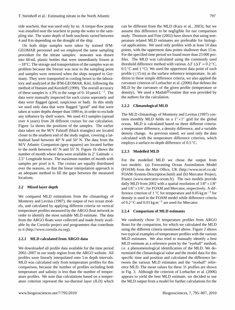
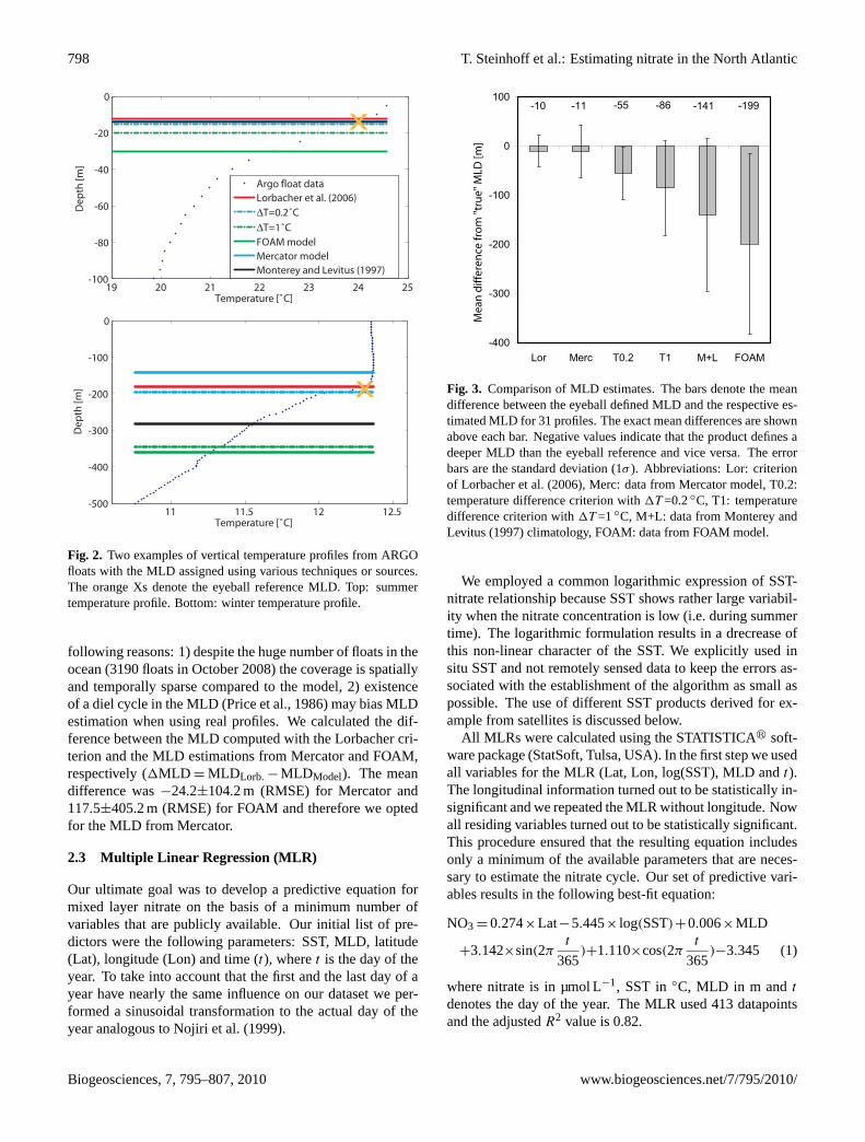
We randomly chose 31 temperature profiles from ARGOfloats for the comparison, for which we calculated the MLDusing the different criteria mentioned above. Figure2 showstwo typical examples of temperature profiles with the variousMLD estimates. We also tried to manually identify a bestMLD estimate as a reference point by the “eyeball” method,i.e. a phenomenological identification of the MLD. We de-termined the climatological value and the model data for thisspecific time and position and calculated the difference be-tween the various MLD estimates and the “eyeball” refer-ence MLD. The mean values for these 31 profiles are shownin Fig. 3. Although the criterion ofLorbacher et al.(2006)appears to yield the best MLD estimate, we decided to usethe MLD output from a model for further calculations for the

www.biogeosciences.net/7/795/2010/ Biogeosciences, 7, 795–807, 2010

http://www.coriolis.eu.org

http://www.ncof.co.uk/FOAM-System-Description.html

http://www.ncof.co.uk/FOAM-System-Description.html

www.mercator-ocean.fr


19 20 21 22 23 24 25-100

-80

-60

-40

-20

0

Temperature [˚C]

]m[

htpe

D

Argo float dataLorbacher et al. (2006)∆T=0.2˚C

∆T=1˚CFOAM modelMercator modelMonterey and Levitus (1997)

11 11.5 12 12.5-500

-400

-300

-200

-100

0

Temperature [˚C]

Dep

th [m

]

x

x

Fig. 2. Two examples of vertical temperature profiles from ARGOfloats with the MLD assigned using various techniques or sources.The orange Xs denote the eyeball reference MLD. Top: summertemperature profile. Bottom: winter temperature profile.

following reasons: 1) despite the huge number of floats in theocean (3190 floats in October 2008) the coverage is spatiallyand temporally sparse compared to the model, 2) existenceof a diel cycle in the MLD (Price et al., 1986) may bias MLDestimation when using real profiles. We calculated the dif-ference between the MLD computed with the Lorbacher cri-terion and the MLD estimations from Mercator and FOAM,respectively (1MLD = MLDLorb. −MLDModel). The meandifference was−24.2±104.2 m (RMSE) for Mercator and117.5±405.2 m (RMSE) for FOAM and therefore we optedfor the MLD from Mercator.

2.3 Multiple Linear Regression (MLR)

Our ultimate goal was to develop a predictive equation formixed layer nitrate on the basis of a minimum number ofvariables that are publicly available. Our initial list of pre-dictors were the following parameters: SST, MLD, latitude(Lat), longitude (Lon) and time (t), wheret is the day of theyear. To take into account that the first and the last day of ayear have nearly the same influence on our dataset we per-formed a sinusoidal transformation to the actual day of theyear analogous toNojiri et al. (1999).

991-68-55-11-01- 141-

004-

003-

002-

001-

0

001

MAOFL+M1T2.0TcreMroL

Mea

n d

iffer

ence

fro

m "

tru

e" M

LD [m

]

Fig. 3. Comparison of MLD estimates. The bars denote the meandifference between the eyeball defined MLD and the respective es-timated MLD for 31 profiles. The exact mean differences are shownabove each bar. Negative values indicate that the product defines adeeper MLD than the eyeball reference and vice versa. The errorbars are the standard deviation (1σ ). Abbreviations: Lor: criterionof Lorbacher et al.(2006), Merc: data from Mercator model, T0.2:temperature difference criterion with1T =0.2◦C, T1: temperaturedifference criterion with1T =1◦C, M+L: data from Monterey andLevitus (1997) climatology, FOAM: data from FOAM model.

We employed a common logarithmic expression of SST-nitrate relationship because SST shows rather large variabil-ity when the nitrate concentration is low (i.e. during summertime). The logarithmic formulation results in a drecrease ofthis non-linear character of the SST. We explicitly used insitu SST and not remotely sensed data to keep the errors as-sociated with the establishment of the algorithm as small aspossible. The use of different SST products derived for ex-ample from satellites is discussed below.

All MLRs were calculated using the STATISTICAr soft-ware package (StatSoft, Tulsa, USA). In the first step we usedall variables for the MLR (Lat, Lon, log(SST), MLD andt).The longitudinal information turned out to be statistically in-significant and we repeated the MLR without longitude. Nowall residing variables turned out to be statistically significant.This procedure ensured that the resulting equation includesonly a minimum of the available parameters that are neces-sary to estimate the nitrate cycle. Our set of predictive vari-ables results in the following best-fit equation:

NO3 = 0.274×Lat−5.445× log(SST)+0.006×MLD

+3.142×sin(2πt

365)+1.110×cos(2π

t

365)−3.345 (1)

where nitrate is in µmol L−1, SST in◦C, MLD in m and t

denotes the day of the year. The MLR used 413 datapointsand the adjustedR2 value is 0.82.



To study possible improvements by adding chl-a datafrom SeaWifs (http://oceancolor.gsfc.nasa.gov) to the initialdataset we performed a MLR with SST, MLD, Lat, Lon, timeand chl-a as predictors. The chl-data were 8 day compositeswith 9km resolution (at the equator). The adjustedR2 valueof the resulting equation is also 0.82. A major drawback ofadding chl-a is the reduction of datapoints for the MLR. Dueto the typical clouds above the North Atlantic the cases werewe had data for nitrate, MLD and chl-a were reduced to 230.Therefore we did not include chl-a in the algorithm.

2.4 Self-Organizing Map (SOM)

The regression coefficients provide information about physi-cal relationships between nitrate and SST or MLD, respec-tively, if the predictors of a MLR are independent. Thedrawback of this method is the limitation to a linear relationand (even for a polynomial regression) the fitting to a pre-defined function. Therefore, a neural network approach wasadditionally employed using a self-organizing map. SOMswere introduced to science byKohonen (1982) and suc-cessfully applied to oceanographic data byLefevre et al.(2005), Friedrich and Oschlies(2009a,b) and Telszewskiet al. (2009). SOMs are able to estimate a target value (e.g.nitrate) from related parameters (e.g. MLD, SST) withoutfitting to a predefined function by recognizing relationshipsin the observational data during the training process. Thesame predictive parameters used in the MLR (Eq.1) wereemployed in the SOM.

2.5 Algorithm validation

2.5.1 Validation against observational data

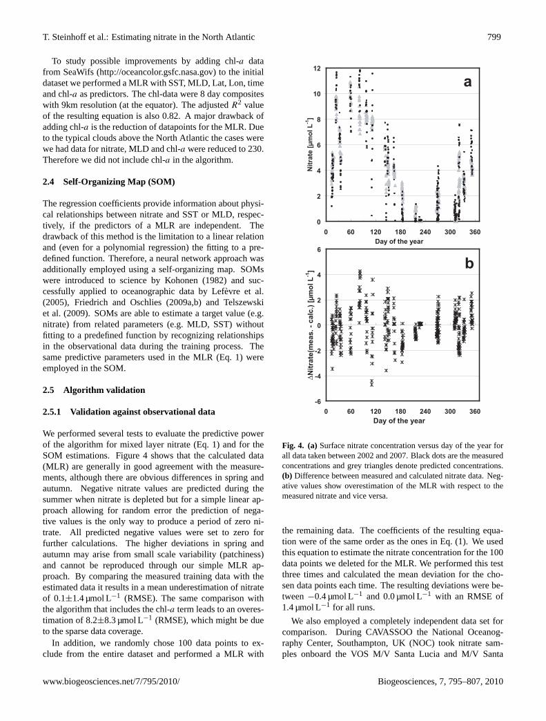
We performed several tests to evaluate the predictive powerof the algorithm for mixed layer nitrate (Eq.1) and for theSOM estimations. Figure4 shows that the calculated data(MLR) are generally in good agreement with the measure-ments, although there are obvious differences in spring andautumn. Negative nitrate values are predicted during thesummer when nitrate is depleted but for a simple linear ap-proach allowing for random error the prediction of nega-tive values is the only way to produce a period of zero ni-trate. All predicted negative values were set to zero forfurther calculations. The higher deviations in spring andautumn may arise from small scale variability (patchiness)and cannot be reproduced through our simple MLR ap-proach. By comparing the measured training data with theestimated data it results in a mean underestimation of nitrateof 0.1±1.4 µmol L−1 (RMSE). The same comparison withthe algorithm that includes the chl-a term leads to an overes-timation of 8.2±8.3 µmol L−1 (RMSE), which might be dueto the sparse data coverage.

In addition, we randomly chose 100 data points to ex-clude from the entire dataset and performed a MLR with

0

2

4

6

8

10

12

0 60 120 180 240 300 360Day of the year

Nitr

ate

[µm

ol L

-1]

a

-6

-4

-2

0

2

4

6

0 60 120 180 240 300 360Day of the year

∆ Nitr

ate(

mea

s. -

calc

.) [µ

mol

L-1

] b

Fig. 4. (a)Surface nitrate concentration versus day of the year forall data taken between 2002 and 2007. Black dots are the measuredconcentrations and grey triangles denote predicted concentrations.(b) Difference between measured and calculated nitrate data. Neg-ative values show overestimation of the MLR with respect to themeasured nitrate and vice versa.

the remaining data. The coefficients of the resulting equa-tion were of the same order as the ones in Eq. (1). We usedthis equation to estimate the nitrate concentration for the 100data points we deleted for the MLR. We performed this testthree times and calculated the mean deviation for the cho-sen data points each time. The resulting deviations were be-tween−0.4 µmol L−1 and 0.0 µmol L−1 with an RMSE of1.4 µmol L−1 for all runs.

We also employed a completely independent data set forcomparison. During CAVASSOO the National Oceanog-raphy Center, Southampton, UK (NOC) took nitrate sam-ples onboard the VOS M/V Santa Lucia and M/V Santa


http://oceancolor.gsfc.nasa.gov


Maria, respectively. Both ships were sailing between theUK and Carribean (Fig.1) and produced more than 600 ni-trate samples between May 2002 and December 2003 in thearea north of 40◦ N. We used the SST from their datasetand the matching MLD from Mercator to estimate corre-sponding nitrate data with both methods: SOM and MLR.Since we do not have the MLD for all 2002 dates we in-cluded only 344 datapoints. In average nitrate was under-estimated by 0.6±1.2 µmol L−1 (RMSE) with the MLR andoverestimated by 0.4±1.5 µmol L−1 (RMSE) with the SOM.Using only data between 10◦ W and 50◦ W (the SOM wastrained only in this region) the MLR underestimates nitrateby 0.5±1.1 µmol L−1 (RMSE) and the SOM overestimates itby 0.3±1.3 µmol L−1 (RMSE).

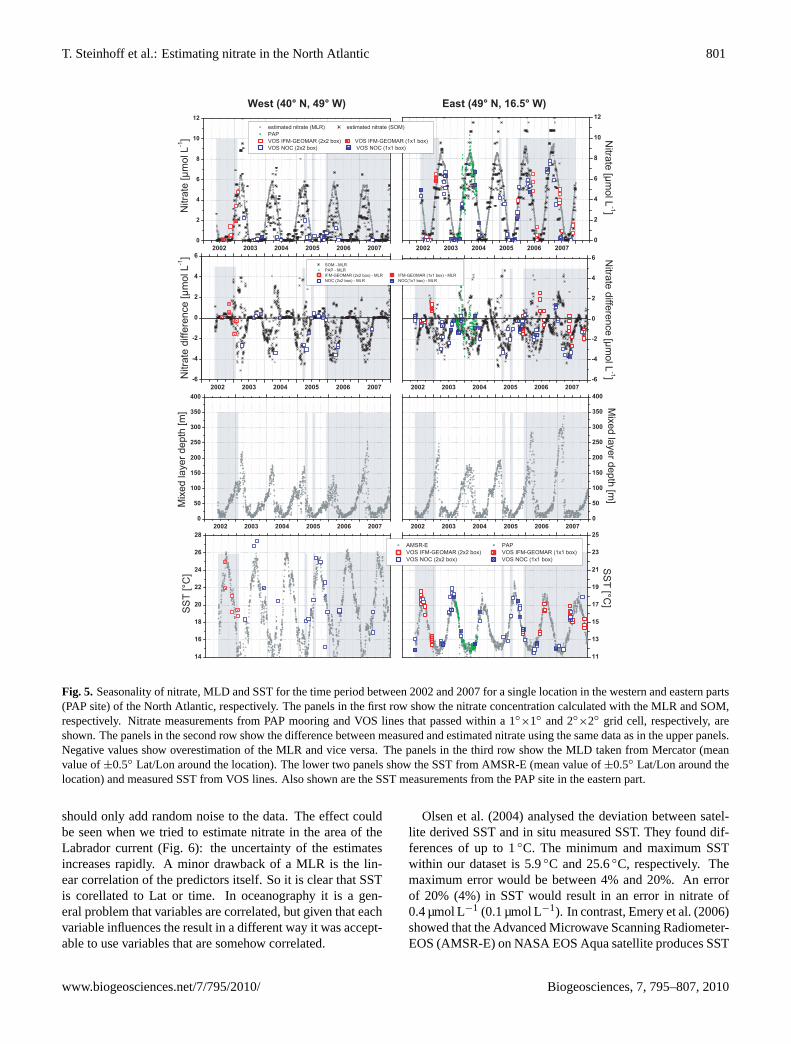
Figure5 shows the intra and interannual variability of SST,MLD and nitrate concentration for the time period between2002 and 2007 for two example locations: eastern (49◦ N,16.5◦ W, PAP) and western (40◦ N, 49◦ W) North Atlantic.SST and nitrate are also available for a whole annual cycle in2002/2003 at the PAP site (Kortzinger et al., 2008), resultingin another independent dataset. The West Atlantic locationwas chosen to illustrate the limitations of a MLR approachbecause the Labrador current may introduce short term vari-ability on a daily timescale. The corresponding SST and ni-trate values measured onboard one of the VOS lines men-tioned above were added to the plot if one of the VOS linecrossed an area of 1◦

×1◦ (2◦×2◦) latitude/longitude around

the location within one day. The annual amplitude of SSTis more pronounced in the western region and the short termvariability is also higher. The VOS SST measurements are ingood agreement with AMSR-E in the eastern region. Devia-tions can be seen in the westerly region due to the high shortterm variability there, especially if data are from a 2◦

×2◦

grid cell. This short term variability at the westerly locationalso results in deviation of the VOS measured nitrate datafrom the predicted concentrations.

The MLD amplitude is slightly higher at PAP station. Theinstruments at PAP were deployed in approximately 30 mdepth andKortzinger et al.(2008) excluded data that weremeasured below the thermocline. The SST data measuredat PAP and from the VOS lines agree with the data fromAMSR-E. This results in good agreement between measure-ments and predicted values of nitrate. In contrast to the mea-sured and SOM estimated nitrate data the (MLR) calculatednitrate data show a smooth seasonality. A comparison of thelatter two results in a RMS error of 0.9 µmol L−1. A compar-ison of the SOM calculated data and the measured values atPAP results in a RMS error of 1.4 µmol L−1. However, theSOM estimates in the western part are in better agreementwith the measured data. Figure5 (second row) shows the dif-ference between MRL estimated nitrate and the other nitrateproducts. The SOM estimates and the VOS measurementsdeviate mostly in the same order and direction.

2.5.2 Validation using a biogeochemical model

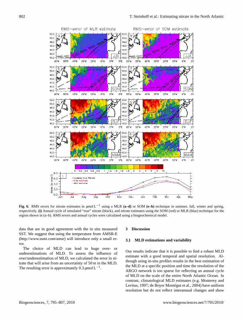
Predicted nitrate concentrations were also validated againstnitrate concentrations predicted by a high-resolutionnitrogen-based nitrate-phytoplankton-zooplankton-detritusmodel of the North Atlantic. All model details are describedin Oschlies et al.(2000) andEden and Oschlies(2006). Theadvantage of this model-based validation is that the modelproduces daily nitrate fields with a horizontal resolution of1/12◦

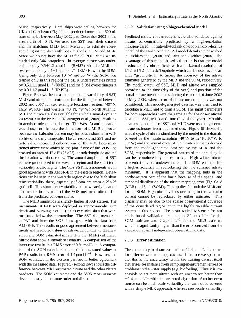
×1/12◦ latitude/longitude which can be used as a basinwide “ground-truth” to assess the accuracy of the nitrateestimates generated by the MLR and the SOM, respectively.The model output of SST, MLD and nitrate was sampledaccording to the time (day of the year) and position of theactual nitrate measurements during the period of June 2002to May 2003, where error of nitrate measurements was notconsidered. This model-generated data set was then used tocalculate a MLR and to train a SOM. The input parametersfor both approaches were the same as for the observationaldata: Lat, SST, MLD and time (day of the year). Monthlymean model outputs of SST and MLD were used to generatenitrate estimates from both methods. Figure6i shows theannual cycle of nitrate simulated by the model in the domaincovered by the nitrate sampling (40◦ N to 52◦ N, 10◦ W to50◦ W) and the annual cycle of the nitrate estimates derivedfrom the model-generated data set by the MLR and theSOM, respectively. The general pattern of the annual cyclecan be reproduced by the estimates. High winter nitrateconcentrations are underestimated. The SOM estimate hasa higher accuracy in reproducing the late summer nitrateminimum. It is apparent that the mapping fails in thenorth-western part of the basin because of the spatial andtemporal distribution of the nitrate mapping error (Fig.6a–d(MLR) and6e–h (SOM)). This applies for both the MLR andfor the SOM. High nitrate values occurring in the Labradorcurrent cannot be reproduced by either estimate. Thisdisparity may be due to the sparse observational coverageof the considered region or to the highly variable currentsystem in this region. The basin wide RMS-error for ourmodel-based validation amounts to 2.1 µmol L−1 for theSOM estimate and 2.2 µmol L−1 for the MLR estimatewhich is significantly higher than the error derived from thevalidation against independent observational data.

2.5.3 Error estimation

The uncertainty in nitrate estimation of 1.4 µmol L−1 appearsfor different validation approaches. Therefore we speculatethat this is the uncertainty within the training dataset itselfthat arises for instance from sampling/measurement errors orproblems in the water supply (e.g. biofouling). Thus it is im-possible to estimate nitrate with an uncertainty better than±1.4 µmol L−1 with the presented algorithm. Another errorsource can be small scale variability that can not be coveredwith a simple MLR approach, whereas mesoscale variability



Fig. 5. Seasonality of nitrate, MLD and SST for the time period between 2002 and 2007 for a single location in the western and eastern parts(PAP site) of the North Atlantic, respectively. The panels in the first row show the nitrate concentration calculated with the MLR and SOM,respectively. Nitrate measurements from PAP mooring and VOS lines that passed within a 1◦

×1◦ and 2◦×2◦ grid cell, respectively, areshown. The panels in the second row show the difference between measured and estimated nitrate using the same data as in the upper panels.Negative values show overestimation of the MLR and vice versa. The panels in the third row show the MLD taken from Mercator (meanvalue of±0.5◦ Lat/Lon around the location). The lower two panels show the SST from AMSR-E (mean value of±0.5◦ Lat/Lon around thelocation) and measured SST from VOS lines. Also shown are the SST measurements from the PAP site in the eastern part.

should only add random noise to the data. The effect couldbe seen when we tried to estimate nitrate in the area of theLabrador current (Fig.6): the uncertainty of the estimatesincreases rapidly. A minor drawback of a MLR is the lin-ear correlation of the predictors itself. So it is clear that SSTis corellated to Lat or time. In oceanography it is a gen-eral problem that variables are correlated, but given that eachvariable influences the result in a different way it was accept-able to use variables that are somehow correlated.

Olsen et al.(2004) analysed the deviation between satel-lite derived SST and in situ measured SST. They found dif-ferences of up to 1◦C. The minimum and maximum SSTwithin our dataset is 5.9◦C and 25.6◦C, respectively. Themaximum error would be between 4% and 20%. An errorof 20% (4%) in SST would result in an error in nitrate of0.4 µmol L−1 (0.1 µmol L−1). In contrast,Emery et al.(2006)showed that the Advanced Microwave Scanning Radiometer-EOS (AMSR-E) on NASA EOS Aqua satellite produces SST



Fig. 6. RMS errors for nitrate estimates in µmol L−1 using a MLR(a–d) or SOM (e–h) technique in summer, fall, winter and spring,respectively.(i) Annual cycle of simulated “true” nitrate (black), and nitrate estimates using the SOM (red) or MLR (blue) technique for theregion shown in (a–h). RMS errors and annual cycles were calculated using a biogeochemical model.

data that are in good agreement with the in situ measuredSST. We suggest that using the temperature from AMSR-E(http://www.ssmi.com/amsr) will introduce only a small er-ror.

The choice of MLD can lead to huge over- orunderestimations of MLD. To assess the influence ofover/underestimation of MLD, we calculated the error in ni-trate that will arise from an uncertainty of 50 m in the MLD.The resulting error is approximately 0.3 µmol L−1.

3 Discussion

3.1 MLD estimations and variability

Our results indicate that it is possible to find a robust MLDestimate with a good temporal and spatial resolution. Al-though using in-situ profiles results in the best estimation ofthe MLD at a specific position and time the resolution of theARGO network is too sparse for reflecting an annual cycleof MLD on the scale of the entire North Atlantic Ocean. Incontrast, climatological MLD estimates (e.g.Monterey andLevitus, 1997; de Boyer Montegut et al., 2004) have uniformresolution but do not reflect interannual changes and show


http://www.ssmi.com/amsr


considerable deviations from observations (e.g. tend to sig-nificantly overpredict MLD). Using MLD generated by mod-els could be a compromise: data are produced on a daily ba-sis, on a regular grid, and can be in good agreement with ob-servations. Here we compare results from two models sincethe model dependent differences are large.

For in-situ profiles, such as those measured by floats, thecurvature criterion ofLorbacher et al.(2006) results in MLDthat are closest to those which are eyeball-defined (Fig.3).The model output from FOAM yields MLD that are sig-nificantly deeper than in-situ observations. This finding isin good agreement withde Boyer Montegut et al.(2004)who, among others, showed that a temperature criterion of1◦C (see Fig.2.2.3) is too large for the subpolar North At-lantic. We chose the model output of the Mercator project, asthis provides high resolution and MLD that are close to theeyeball-defined MLD.

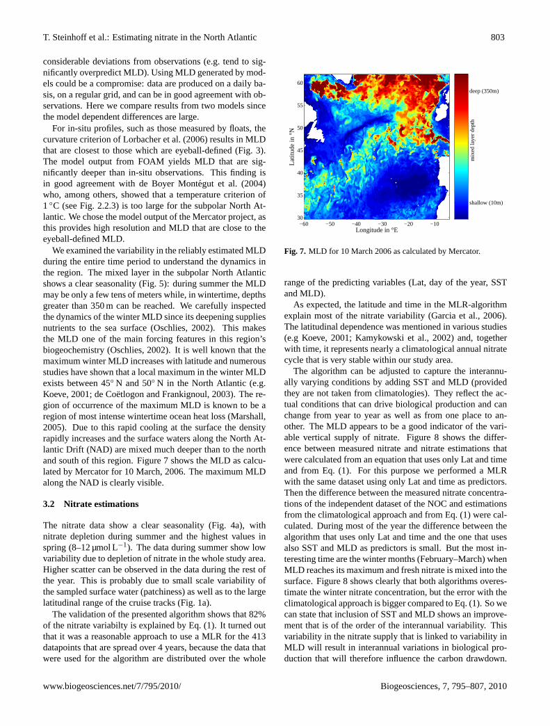
We examined the variability in the reliably estimated MLDduring the entire time period to understand the dynamics inthe region. The mixed layer in the subpolar North Atlanticshows a clear seasonality (Fig.5): during summer the MLDmay be only a few tens of meters while, in wintertime, depthsgreater than 350 m can be reached. We carefully inspectedthe dynamics of the winter MLD since its deepening suppliesnutrients to the sea surface (Oschlies, 2002). This makesthe MLD one of the main forcing features in this region’sbiogeochemistry (Oschlies, 2002). It is well known that themaximum winter MLD increases with latitude and numerousstudies have shown that a local maximum in the winter MLDexists between 45◦ N and 50◦ N in the North Atlantic (e.g.Koeve, 2001; de Coetlogon and Frankignoul, 2003). The re-gion of occurrence of the maximum MLD is known to be aregion of most intense wintertime ocean heat loss (Marshall,2005). Due to this rapid cooling at the surface the densityrapidly increases and the surface waters along the North At-lantic Drift (NAD) are mixed much deeper than to the northand south of this region. Figure7 shows the MLD as calcu-lated by Mercator for 10 March, 2006. The maximum MLDalong the NAD is clearly visible.

3.2 Nitrate estimations

The nitrate data show a clear seasonality (Fig.4a), withnitrate depletion during summer and the highest values inspring (8–12 µmol L−1). The data during summer show lowvariability due to depletion of nitrate in the whole study area.Higher scatter can be observed in the data during the rest ofthe year. This is probably due to small scale variability ofthe sampled surface water (patchiness) as well as to the largelatitudinal range of the cruise tracks (Fig.1a).

The validation of the presented algorithm shows that 82%of the nitrate variabilty is explained by Eq. (1). It turned outthat it was a reasonable approach to use a MLR for the 413datapoints that are spread over 4 years, because the data thatwere used for the algorithm are distributed over the whole

−60 −50 −40 −30 −20 −1030

35

40

45

50

55

60

Longitude in °E

Lat

itude

in °

N

shallow (10m)

deep (350m)

mix

ed la

yer

dept

h

Fig. 7. MLD for 10 March 2006 as calculated by Mercator.

range of the predicting variables (Lat, day of the year, SSTand MLD).

As expected, the latitude and time in the MLR-algorithmexplain most of the nitrate variability (Garcia et al., 2006).The latitudinal dependence was mentioned in various studies(e.g Koeve, 2001; Kamykowski et al., 2002) and, togetherwith time, it represents nearly a climatological annual nitratecycle that is very stable within our study area.

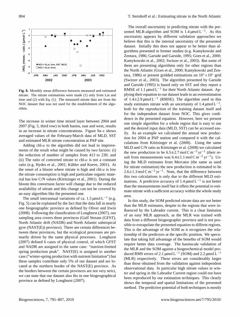
The algorithm can be adjusted to capture the interannu-ally varying conditions by adding SST and MLD (providedthey are not taken from climatologies). They reflect the ac-tual conditions that can drive biological production and canchange from year to year as well as from one place to an-other. The MLD appears to be a good indicator of the vari-able vertical supply of nitrate. Figure8 shows the differ-ence between measured nitrate and nitrate estimations thatwere calculated from an equation that uses only Lat and timeand from Eq. (1). For this purpose we performed a MLRwith the same dataset using only Lat and time as predictors.Then the difference between the measured nitrate concentra-tions of the independent dataset of the NOC and estimationsfrom the climatological approach and from Eq. (1) were cal-culated. During most of the year the difference between thealgorithm that uses only Lat and time and the one that usesalso SST and MLD as predictors is small. But the most in-teresting time are the winter months (February–March) whenMLD reaches its maximum and fresh nitrate is mixed into thesurface. Figure8 shows clearly that both algorithms overes-timate the winter nitrate concentration, but the error with theclimatological approach is bigger compared to Eq. (1). So wecan state that inclusion of SST and MLD shows an improve-ment that is of the order of the interannual variability. Thisvariability in the nitrate supply that is linked to variability inMLD will result in interannual variations in biological pro-duction that will therefore influence the carbon drawdown.



-6

-5

-4

-3

-2

-1

0

1

∆ NO

3 (m

eas.

- ca

lc.)

[µm

ol L

-1]

NO3 = f(Lat, time, SST, MLD)NO3 = f(Lat, time)

2002 2003JFM AMJ JAS OND JFM AMJ JAS OND

Fig. 8. Monthly mean difference between measured and estimatednitrate. The nitrate estimations were made (1) only from Lat andtime and (2) with Eq. (1). The measured nitrate data are from theNOC dataset that was not used for the establishment of the algo-rithm.

The increase in winter time mixed layer between 2004 and2007 (Fig.5, third row) in both basins, east and west, resultsin an increase in nitrate concentrations. Figure9a–c showsaveraged values of the February/March data of MLD, SSTand estimated MLR nitrate concentration at PAP site.

Adding chl-a to the algorithm did not lead to improve-ments of the result what might be caused by two factors: (i)the reduction of number of samples from 413 to 230; and(ii) The ratio of converted nitrate to chl-a is not a constantratio (e.g.Hydes et al., 2001; Kahler and Koeve, 2001). Atthe onset of a bloom where nitrate is high and chl-a is lowthe nitrate consumption is high and particulate organic mate-rial has low C/N values (Kortzinger et al., 2001). During thebloom this conversion factor will change due to the reducedavailability of nitrate and this change can not be covered byan easy algorithm like the presented one.

The small interannual variations of ca. 1.5 µmol L−1 (e.g.Fig.5) can be explained by the fact that the data fall in nearlyone biogeographic province as defined byOliver and Irwin(2008). Following the classification ofLonghurst(2007), oursampling area covers three provinces (Gulf Stream (GFST),North Atlantic drift (NADR) and North Atlantic subtropicalgyre (NAST(E)) province). There are certain differences be-tween these provinces, but the ecological processes are pri-marily driven by the same physical processes.Longhurst(2007) defined 6 cases of physical control, of which GFSTand NADR are assigned to the same case: “nutrient-limitedspring production peak”. NAST(E) is assigned to anothercase (“winter-spring production with nutrient limitation”) butthese samples contribute only 5% of our dataset and are lo-cated at the northern border of the NAST(E) province. Asthe borders between the certain provinces are not very strict,we can state that our dataset also fits in one biogeographicalprovince as defined byLonghurst(2007).

The overall uncertainty in predicting nitrate with the pre-sented MLR-algorithm and SOM is 1.4 µmol L−1. As thisuncertainty appears by different validation approaches webelieve that this is the internal uncertainty of the presenteddataset. Initially this does not appear to be better than al-gorithms presented in former studies (e.g.Kamykowski andZentara, 1986; Garside and Garside, 1995; Goes et al., 2000;Kamykowski et al., 2002; Switzer et al., 2003). But some ofthem are presenting algorithms only for other regions thanthe North Atlantic (Goes et al., 2000; Kamykowski and Zen-tara, 1986) or present gridded estimations on 10◦

×10◦ grid(Switzer et al., 2003). The algorithm presented byGarsideand Garside(1995) is based only on SST and they report aRMSE of 1.1 µmol L−1 for their North Atlantic dataset. Ap-plying their equation to our dataset leads to an overestimationof 1.4±2.9 µmol L−1 (RMSE). The algorithm used in thisstudy estimates nitrate with an uncertainty of 1.4 µmol L−1,both for the reproduction of the training dataset itself andfor the independent dataset from NOC. This gives confi-dence in the presented equation. However, here we presentone simple algorithm for a whole region that is easy to useand the desired input data (MLD, SST) can be accessed eas-ily. As an example we calculated the annual new produc-tion for 2004 at PAP station and compared it with the cal-culations fromKortzinger et al.(2008). Using the sameMLD and C/N ratio asKortzinger et al.(2008) we calculatedthe new production to be 6.5±2.7 mol C m−2 yr−1 (their re-sult from measurements was 6.4±1.1 mol C m−2 yr−1). Us-ing the MLD estimates from Mercator (the same as usedfor nitrate estimation) the new production is estimated to be2.6±1.3 mol C m−2 yr−1. Note, that the difference betweenthis two calculations is only due to the different MLD esti-mations. A predictive accuracy of 1.4 µmol L−1 is not betterthan the measurements itself but it offers the potential to esti-mate nitrate with a sufficient accuracy within the whole studyarea.

In this study, the SOM predicted nitrate data are not betterthan the MLR estimates, despite in the regions that were in-fluenced by the Labrador current. This is a clear limitaionof an easy MLR approach, as the MLR was trained withdata from a different biogeographic province and is not pos-sible to extrapolate the presented equation to differnt regions.This is the advantage of the SOM as it recognizes the rela-tionship of the predictors at the specific position. We specu-late that taking full advantage of the benefits of SOM wouldrequire better data coverage. The basinscale validation ofthe MLR and the SOM against a biogeochemical model pro-duced RMS errors of 2.1 µmol L−1 (SOM) and 2.2 µmol L−1

(MLR) respectively. These errors are considerably largerthan those obtained from the validation against independentobservational data. In particular high nitrate values in win-ter and spring in the Labrador Current region could not havebeen reproduced by our estimation techniques. This clearlyshows the temporal and spatial limitations of the presentedmethod. The predictive potential of both techniques is mostly



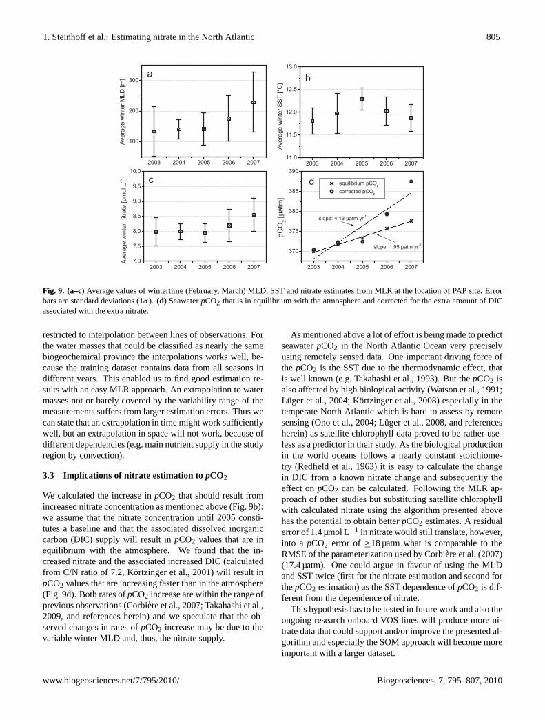
Fig. 9. (a–c)Average values of wintertime (February, March) MLD, SST and nitrate estimates from MLR at the location of PAP site. Errorbars are standard deviations (1σ ). (d) SeawaterpCO2 that is in equilibrium with the atmosphere and corrected for the extra amount of DICassociated with the extra nitrate.

restricted to interpolation between lines of observations. Forthe water masses that could be classified as nearly the samebiogeochemical province the interpolations works well, be-cause the training dataset contains data from all seasons indifferent years. This enabled us to find good estimation re-sults with an easy MLR approach. An extrapolation to watermasses not or barely covered by the variability range of themeasurements suffers from larger estimation errors. Thus wecan state that an extrapolation in time might work sufficientlywell, but an extrapolation in space will not work, because ofdifferent dependencies (e.g. main nutrient supply in the studyregion by convection).

3.3 Implications of nitrate estimation to pCO2

We calculated the increase inpCO2 that should result fromincreased nitrate concentration as mentioned above (Fig.9b):we assume that the nitrate concentration until 2005 consti-tutes a baseline and that the associated dissolved inorganiccarbon (DIC) supply will result inpCO2 values that are inequilibrium with the atmosphere. We found that the in-creased nitrate and the associated increased DIC (calculatedfrom C/N ratio of 7.2,Kortzinger et al., 2001) will result inpCO2 values that are increasing faster than in the atmosphere(Fig.9d). Both rates ofpCO2 increase are within the range ofprevious observations (Corbiere et al., 2007; Takahashi et al.,2009, and references herein) and we speculate that the ob-served changes in rates ofpCO2 increase may be due to thevariable winter MLD and, thus, the nitrate supply.

As mentioned above a lot of effort is being made to predictseawaterpCO2 in the North Atlantic Ocean very preciselyusing remotely sensed data. One important driving force ofthe pCO2 is the SST due to the thermodynamic effect, thatis well known (e.g.Takahashi et al., 1993). But thepCO2 isalso affected by high biological activity (Watson et al., 1991;Luger et al., 2004; Kortzinger et al., 2008) especially in thetemperate North Atlantic which is hard to assess by remotesensing (Ono et al., 2004; Luger et al., 2008, and referencesherein) as satellite chlorophyll data proved to be rather use-less as a predictor in their study. As the biological productionin the world oceans follows a nearly constant stoichiome-try (Redfield et al., 1963) it is easy to calculate the changein DIC from a known nitrate change and subsequently theeffect onpCO2 can be calculated. Following the MLR ap-proach of other studies but substituting satellite chlorophyllwith calculated nitrate using the algorithm presented abovehas the potential to obtain betterpCO2 estimates. A residualerror of 1.4 µmol L−1 in nitrate would still translate, however,into a pCO2 error of ≥18 µatm what is comparable to theRMSE of the parameterization used byCorbiere et al.(2007)(17.4 µatm). One could argue in favour of using the MLDand SST twice (first for the nitrate estimation and second forthepCO2 estimation) as the SST dependence ofpCO2 is dif-ferent from the dependence of nitrate.

This hypothesis has to be tested in future work and also theongoing research onboard VOS lines will produce more ni-trate data that could support and/or improve the presented al-gorithm and especially the SOM approach will become moreimportant with a larger dataset.



Acknowledgements.We thank the captains and crews of M/VFalstaff, M/V Atlantic Companion, M/V Santa Maria and M/VSanta Lucia for their support. We would also like to thank allthe people involved in taking/measuring the nitrate samples.Mooring data and support for this research were provided bythe European research projects ANIMATE (Atlantic Network ofInterdisciplinary Moorings and Time-Series for Europe), MERSEA(Marine Environment and Security for the European Sea) andEUR-OCEANS (European Network of Excellence for OceanEcosystems Analysis). This route of M/V Santa Maria and M/VSanta Lucia is used by the CAVASSOO (Carbon Variability Studiesby Ships Of Opportunity) project to investigate seasonal andyear-to-year variations in carbon fluxes in the North Atlantic. Moreinformation on CAVASSOO (EC funded between Nov 2000 andNov 2003, EC grant number EVK2-CT-2000-00088) is availableon: http://tracer.env.uea.ac.uk/e072/. This work was supportedby the European Commission under the CARBOOCEAN projectGOCE 511176-2. The authors thank the Ocean Biology ProcessingGroup (Code 614.2) at the GSFC, Greenbelt, MD 20771, forthe production and distribution of the ocean color data. Twoanonymous reviewer provided helpful comments.

Edited by: S. W. A. Naqvi

References

Bates, N. R.: Interannual variability of the oceanic CO2 sinkin the subtropical gyre of the North Atlantic Ocean over thelast 2 decades, J. Geophys. Res., 112, C09013, doi:10.1029/2006JC003759, 2007.

Chierici, M., Olsen, A., Johannessen, T., Trinanes, J., and Wan-ninkhof, R.: Algorithms to estimate the carbon dioxide uptake inthe northern North Atlantic using shipboard observations, satel-lite and ocean analysis data, Deep-Sea Res. II, 56, 630–639,2009.

Cianca, A., Helmke, P., Mourino, B., Rueda, M. J., Llinas,O., and Neuer, S.: Decadal analysis of hydrography andin situ nutrient budgets in the western and eastern NorthAtlantic subtropical gyre, J. Geophys. Res., 112, C07025,doi:10.1029/2006JC003788, 2007.

Corbiere, A., Metzl, N., Reverdin, G., Brunet, C., and Takahashi,T.: Interannual and decadal variability of the oceanic carbon sinkin the North Atlantic subpolar gyre, Tellus, 59B, 168–178, 2007.

de Boyer Montegut, C., Madec, G., Fischer, A. S., Lazar, A., andIudicone, D.: Mixed layer depth over the global ocean: An exam-ination of profile data and profile-based climatology, J. Geophys.Res., 109, C12003, doi:10.1029/2004JC002378, 2004.

de Coetlogon, G. and Frankignoul, C.: The persistence of WinterSea Surface Temperature in the North Atlantic, J. Climate, 16,1364–1377, 2003.

Eden, C. and Oschlies, A.: Adiabatic reduction of circulation-related CO2 air-sea flux biases in a North Atlantic carbon-cycle model, Global Biogeochem. Cy., 20, GB2008,doi:10.1029/2005GB002521, 2006.

Emery, W., Brandt, P., Funk, A., and Boning, C.: A comparison ofsea surface temperatures from microwave remote sensing of theLabrador Sea with in situ measurements and model simulations,J. Geophys. Res., 111, C12013, doi:10.1029/2006JC003578,2006.

Friedrich, T. and Oschlies, A.: Neural network-based esti-mates of North Atlantic surfacepCO2 from satellite data:A methodological study, J. Geophys. Res., 114, C03020,doi:10.1029/2007JC004646, 2009a.

Friedrich, T. and Oschlies, A.: Basin-scalepCO2 maps estimatedfrom ARGO float data – a model study, J. Geophys. Res., 114,C10012, doi:10.1029/2009JC005322, 2009b.

Garcia, H., Locarnini, R., Boyer, T., and Antonov, J.: Volume 4:Nutrients (phosphate, nitrate, silicate), in: World Ocean Atlas2005, edited by: Ed. NOAA Atlas NESDIS 64, U. G. P. O., S.Levitus, 2006.

Garside, C. and Garside, J. C.: Euphotic-zone nutrient algorithmsfor the NABE and EqPac study site, Deep-Sea Res.II, 42, 335–347, 1995.

Glover, D. M. and Brewer, P. G.: Estimates of wintertime mixedlayer nutrient concentration in the North Atlantic, Deep-SeaRes., 35, 1525–1546, 1988.

Goes, J. I., Saino, T., Oaku, H., Ishizaka, J., Wong, C. S., and Nojiri,Y.: Basin scale estimates of sea surface nitrate and new produc-tion from remotely sensed sea surface temperature and chloro-phyll, Geophys. Res. Lett., 27, 1263–1266, 2000.

Gonzalez-Davila, M., Santana-Casiano, J. M., and Gonzalez-Davila, E. F.: Interannual variability of the upper ocean carboncycle in the northeast Atlantic Ocean, Geophys. Res. Lett., 34,L07608, doi:10.1029/2006GL028145, 2007.

Hansen, H. and Koroleff, F.: Determination of nutrients, in: Meth-ods of seawater analysis, edited by: Grasshoff, K., Kremling, K.,and Erhardt, M., Verlag Chemie, Weinheim, Germany, 159–228,1999.

Hartman, S. E., Larkin, K. E., Lampitt, R. S., Lankhorst, M., andHydes, D. J.: Seasonal and inter-annual biogeochemical varia-tions in the Porcupine Abyssal Plain 2003-2005 associated withwinter mixing and surface circulation, Deep Sea Res. II, In Press,doi: 10.1016/j.dsr2.2010.01.007, 2010.

Hydes, D., Gall, A. L., Miller, A., Brockmann, U., Raabe, T., Hol-ley, S., Alvarez-Salgado, X., Antia, A., Balzer, W., L.Chou,Elskens, M., Helder, W., Joint, I., and Orren, M.: Supply anddemand of nutrients and dissolved organic matter at and acrossthe NW European shelf break in relation to hydrography and bio-geochemical activity, Deeep-Sea Res. II, 48, 3023–3047, 2001.

Jamet, C., Moulin, C., and Lefevre, N.: Estimation of the oceanicpCO2 in the North Atlantic from VOS lines in-situ measure-ments: parameters needed to generate seasonally mean maps,Ann. Geophys., 25, 2247–2257, 2007,http://www.ann-geophys.net/25/2247/2007/.

Kahler, P. and Koeve, W.: Marine dissolved organic matter: can itsC:N Ratio explain carbon overconsumption?, Deep Sea Res. I,48, 49–62, 2001.

Kamykowski, D. and Zentara, S.-J.: Predicting plant nutrient con-centration from temperature and sigma-t in the upper Kilometerof the world ocean, Deep-Sea Res. A, 33, 89–105, 1986.

Kamykowski, D., Zentara, S.-J., Morrison, J. M., and Switzer,A. C.: Dynamic global patterns of nitrate, phosphate, sil-icate, and iron, Global Biogeochem. Cy., 16(4), 1077,doi:10.1029/2001GB001640, 2002.

Kara, A. B., Rochford, P. A., and Hurlburt, H. E.: Mixed layer depthvariability over the global ocean, J. Geophys. Res., 108(C3),3079, doi:10.1029/2000JC000736, 2003.

Koeve, W.: Wintertime nutrients in the Noth Atlantic – new ap-


http://tracer.env.uea.ac.uk/e072/

http://www.ann-geophys.net/25/2247/2007/


proaches and implications for new production estimates, Mar.Chem., 74, 245–260, 2001.

Kohonen, T.: Self-Organized Formation of Topologically CorrectFeature Maps, Biol. Cybern., 43, 59–69, 1982.

Kortzinger, A., Koeve, W., Kahler, P., and Mintrop, L.: C:N ratiosin the mixed layer during the productive season in the northeastAtlantic Ocean, Deep-sea Res.I, 48, 661–688, 2001.

Kortzinger, A., Send, U., Lampitt, R. S., Hartman, S., Wallace, D.W. R., Karstensen, J., Villagarcia, M. G., Llinas, O., and De-Grandpre, M. D.: The seasonalpCO2 cycle at 49◦ N/16.5◦ Win the northeastern Atlantic Ocean and what it tells us aboutbiological productivity, J. Geophys. Res., 113, C04020, doi:10.1029/2007JC004347, 2008.

Lefevre, N., Watson, A. J., and Watson, A. R.: A comparison ofmultiple regression and neural network techniques for mappingin situpCO2 data, Tellus, 57B, 375–384, 2005.

Longhurst, A. R.: Ecological geography of the sea, Academic Press,Boston, 2nd edn., 2007.

Lorbacher, K., Dommenget, D., Niiler, P., and Kohl, A.: Oceanmixed layer depth: A subsurface proxy of ocean-atmospherevariability, J. Geophys. Res., 111, C07010, doi:10.1029/2003JC002157, 2006.

Luger, H., Wallace, D. W. R., Kortzinger, A., and Nojiri, Y.: ThepCO2 varability in the midlatitude North Atlantic Ocean duringa full annual cycle, Global Biochem. Cy., 18, GB3023, doi:10.1029/2003GB002200, 2004.

Luger, H., Wanninkhof, R., Olsen, A., Trinanes, J., Johannessen,T., Wallace, D., and Kortzinger, A.: The sea-air CO2 flux in theNorth Atlantic estimated from sattelite and ARGO profiling data,Tech. rep., NOAA, OAR AOML-96, 2008.

Marshall, J.: CLIMODE: a mode water dynamics experiment insupport of CLIVAR, Clivar Variations, 3, No. 2, 8–14, 2005.

Minas, H. J. and Codespoti, L. A.: Estimates of primary productionby observation of changes in the mesoscale nitrate field, ICESMar. Sci. Symp., 197, 215–235, 1993.

Monterey, G. and Levitus, S.: Seasonal Variability of the MixedLayer Depth for the World Ocean, in: NOAA Atlas NESDIS 14,US Gov. Printing Office, Wash., DC, 1997.

Nojiri, Y., Fujinuma, Y., Zeng, J., and Wong, C.: Monitoring ofpCO2 with complete seasonal coverage utilizing a cargo shipM/S Skaugran between Japan and Canada/US, in: Proceed-ings of the 2nd International Symposium CO2 in the Oceans,CGER/NIES, 1999.

Oliver, M. J. and Irwin, A. J.: Objective global ocean biogeographicprovinces, Geoph. Res. Lett., 35, L15601, doi:10.1029/2008/GL034238, 2008.

Olsen, A., Trinanes, J. A., and Wanninkhof, R.: Sea-air flux ofCO2in the Caribbean Sea estimated using in situ and remote sensingdata, Remote Sens. Environ., 89, 309–325, 2004.

Ono, T., Saino, T., Kurita, N., and Sasaki, K.: Basin-scale extrapo-lation of shipboardpCO2 data by using satellite SST and Chla,Int. J. Remote. Sens., 25(19), 3803–3815, 2004.

Oschlies, A.: Nutrient supply to the surface waters of the NorthAtlantic: A model study, J. Geophys. Res., 107, 3046, doi:10.1029/2000JC000275, 2002.

Oschlies, A., Koeve, W., and Garcon, V.: An eddy-permitting cou-pled physical-biological model of the North Atlantic. Part 2:Ecosystem dynamics and comparison with satellite and JGOFSlocal studies data, Global Biogeochem. Cy., 14, 499–523, 2000.

Price, J. F., Weller, R. A., and Pinkel, R.: Diurnal Cycling: Obser-vations and Models of the Upper Ocean Response to, J. Geophys.Res., 91, 8411–8427, 1986.

Redfield, A. C., Ketchum, B. H., and Richards, F. A.: The influenceof organisms on the composition of seawater, in: The Sea, Vol.2,edited by: Hill, M., vol. 2, 26–77, Interscience, New York, 1963.

Sherlock, V., Pickmere, S., Currie, K., Hadfield, M., Nodder, S., andBoyd, P. W.: Predictive accuracy of temperature-nitrate relation-ships for the oceanic mixed layer of the New Zealand region, J.Geophys. Res., 112, C06010, doi:10.1029/2006JC003562, 2007.

Switzer, A. C., Kamykowski, D., and Zentara, S.-J.: Mappingnitrate in the global ocean using remotely sensed sea surfacetemperature, J. Geophys. Res., 108(C8), 3280, doi:10.1029/2000JC000444, 2003.

Takahashi, T., Broeker, W. S., and Langer, S.: Redfield Ratio Basedon Chemical Data from Isopycnal Surfaces, J. Geophys. Res., 90,6907–6924, 1985.

Takahashi, T., Olafsson, J., Goddard, J. G., Chipman, D. W., andSutherland, S. C.: Seasonal Variation of CO2 and Nutrients inthe High-Latitude Surface Oceans: a comparative study, GlobalBiogeochem. Cy., 7, 843–878, 1993.

Takahashi, T., Sutherland, S. C., Wanninkhof, R., Sweeney, C.,Feely, R. A., Chipman, D. W., Hales, B., Friederich, G., Chavez,F., Sabine, C., Watson, A., Bakker, D. C., Schuster, U., Metzl,N., Yoshikawa-Inoue, H., Ishii, M., Midorikawa, T., Nojiri,Y., Kortzinger, A., Steinhoff, T., Hoppema, M., Olafsson,J., Arnarson, T. S., Tilbrook, B., Johannessen, T., Olsen, A.,Bellerby, R., Wong, C., Delille, B., Bates, N., and de Baar,H. J.: Climatological mean and decadal change in surface oceanpCO2, and net sea-air CO2 flux over the global oceans, DeepSea Res. II, 56, 554–577, doi:10.1016/j.dsr2.2008.12.009,http://www.sciencedirect.com/science/article/B6VGC-4V59VVH-1/2/6c157bd4052048ac211736c038787a3a, surface Ocean CO2Variability and Vulnerabilities, 2009.

Telszewski, M., Chazottes, A., Schuster, U., Watson, A. J., Moulin,C., Bakker, D. C. E., Gonzalez-Davila, M., Johannessen, T.,Kortzinger, A., Luger, H., Olsen, A., Omar, A., Padin, X. A.,Rıos, A. F., Steinhoff, T., Santana-Casiano, M., Wallace, D. W.R., and Wanninkhof, R.: Estimating the monthlypCO2 distribu-tion in the North Atlantic using a self-organizing neural network,Biogeosciences, 6, 1405–1421, 2009,http://www.biogeosciences.net/6/1405/2009/.

Thomson, R. E. and Fine, I. V.: Estimating Mixed Layer Depthfrom Oceanic Profile Data, J. Atmos. Ocean. Tech., 20, 319–329,2002.

Watson, A. J., Robinson, C., Robinson, J., Williams, P., andFasham, M.: Spatial variability in the sink for atmospheric car-bon dioxide in the North Atlantic, Nature, 350, 50–53, 1991.


http://www.sciencedirect.com/science/article/B6VGC-4V59VVH-1/2/6c157bd4052048ac211736c038787a3a



http://www.biogeosciences.net/6/1405/2009/

Documents

Estimating mixed layer nitrate in the North Atlantic Ocean · 1Leibniz Institut fur Meereswissenschaften (IFM-GEOMAR), Kiel, Germany¨ 2International Paciﬁc Research Center, School