Estimating Rate Constants of Chemical Reactions using ...three-mode.leidenuniv.nl/bibliogr/bijlsmas_thesis/thesisbijlsma.pdf · Estimating Rate Constants of Chemical Reactions using

Estimating Rate Constantsof Chemical Reactions

using Spectroscopy

Sabina Bijlsma2000

��

��

Printing: Ponsen & Looijen b.v. (Wageningen, The Netherlands)

��

��

ACADEMISCH PROEFSCHRIFT

ter verkrijging van de graad van doctor

aan de Universiteit van Amsterdam

op gezag van de Rector Magnificus

prof. dr. J.J.M. Franse

ten overstaan van een door het college voor promoties ingestelde

commissie in het openbaar te verdedigen in de Aula der Universiteit

op donderdag 22 juni 2000 te 10.00 uur

door

��

geboren te Amsterdam

Promotor : prof. dr. A.K. Smilde, University of Amsterdam

Other committee members : prof. dr. A. Bliek, University of Amsterdam

prof. dr. L.M.C. Buydens, Catholic University of

Nijmegen

prof. dr. H.A.L. Kiers, University of Groningen

prof. dr. G.J. Koomen, University of Amsterdam

prof. dr. P.J. Schoenmakers, University of Amsterdam

dr. R. Tauler, University of Barcelona, Spain

Faculty: : Faculty of Science

��

i

��

�� v

�� vii

��

1.1 Short overview of the history of chemical kinetics 1

1.2 Experimental techniques in kinetics 3

1.3 Spectroscopy 4

1.4 Multivariate analysis tools 5

1.5 Constraints in kinetics 6

1.6 Goal of the thesis 6

1.7 Structure of the thesis 7

1.8 References 7

��

2.1 Introduction 11

2.2 The measurement model 11

2.3 Traditional curve fitting 13

2.4 Fixed-size window evolving factor analysis 15

2.5 Classical curve resolution 16

2.6 Weighted curve resolution 18

2.7 Implementation of constraints 20

2.8 References 20

��!��

3.1 Introduction 23

3.2 Shifting an exponential function 23

3.3 The trilinear structure 24

3.4 Non-iterative three-way methods 31

3.5 Iterative three-way methods 33

3.6 The relative fit error 36

3.7 Implementation of constraints 36

3.8 References 37

��

ii

��"��#�� $��%��%��&��$��

4.1 Introduction 39

4.2 Accuracy of reaction rate constant estimates 39

4.3 A jackknife based method 40

4.4 References 40

��'��(��(��&)��$��*��+�

5.1 Introduction 41

5.2 A two-step epoxidation reaction

5.2.1 Description of the reaction 41

5.2.2 Sample preparation 42

5.2.3 Experimental set-up 43

5.2.4 Dataprocessing 44

5.2.5 The repeatability of experiments 45

5.3 A two-step biochemical reaction

5.3.1 Description of the reaction 45

5.3.2 Sample preparation 46

5.3.3 Experimental set-up 47

5.3.4 Pure spectra 48

5.3.5 Dataprocessing 49

5.3.6 The repeatability of experiments 50

5.4 References 50

��,��

6.1 Introduction 51

6.2 SW-NIR data

6.2.1 Introduction 51

6.2.2 Simulation set-up 52

6.2.3 Results and discussion 53

6.2.4 Conclusions 57

6.3 UV-Vis data (1)




6.4 UV-Vis data (2)




��

iii

6.5 General conclusions 71

6.6 References 72

��-��

7.1 Introduction 73

7.2 SW-NIR data





7.3 UV-Vis data





7.5 References 85

��.��$��/��

8.1 Introduction 87

8.2 SW-NIR and UV-Vis data




��0��+��%��

9.1 Introduction 97

9.2 UV-Vis data





��1��2��3


10.2 Future work 115

10.3 References 116

��

iv

��)

A. Short summary of the datasets 117

B. The proof for a unique solution of the curve resolution model 118

*�$$�� 121

*�$��4 125

5��6�� 129

(�3�� 131

v

��

CCR Classical curve resolution

CR Curve resolution

DECRA Direct exponential curve resolution algorithm

FSWEFA Fixed size window evolving factor analysis

GEP Generalized eigenvalue problem

GRAM Generalized rank annihilation method

GRAM-LM-PAR Generalized rank annihilation method-

Levenberg-Marquardt-parallel factor analysis

HELP Heuristic evolving latent projection

MCR Multivariate curve resolution

PARAFAC Parallel factor analysis

RFE Relative fit error

SSQ Sum of squares

SVD Singular value decomposition

SW-NIR Short-wavelength near-infrared

TCF Traditional curve fitting

TFA Target factor analysis

TLD Trilinear decomposition

TLD-LM-PAR Trilinear decomposition-Levenberg-Marquardt-

parallel factor analysis

UV-Vis Ultraviolet visible

WCR Weighted curve resolution

WLS Weighted least squares

��

vi

vii

��

In general, boldface capital characters denote matrices and boldface lower case

characters denote vectors.

� ((�-�)×3) The matrix with concentration profiles obtained from a GEP

��M� ((�-�)×3) The matrix � after the �th iteration~� ((�-�)×3) The new matrix � obtained by an initial estimate for �1 and �2

~~� ((�-�)×2) The first two columns of matrix

~�

�L The �th column of matrix �

�L�M� The �th column of matrix � after the �th iteration

� ((�+1)×3) The matrix with combined spectra obtained from a GEP

(2×3) The matrix with scaling factors obtained from a GEP

�8�� The initial concentration of species �

�8�L The concentration of species � at time point �; �:�L and �<�L

for and , respectively

(�×�) Matrix with pure spectra

� (�×�) Matrix with spectral residuals

�* ((�-�)×(�+1)×2) Three-way array with spectral residuals

� (�×�) Matrix with concentration profiles

� The step size parameter

� Number of reacting absorbing species

�a, �b Second order reaction rate constants

�1, �2 (Pseudo-) first order reaction rate constants

� Equals )( 12

1

��−

1� , 2� Mean estimated �1 and �2 calculated over the individual

estimates

� Number of time points

� Number of wavelengths

� The time shift parameter

L The time at point �

(�×�) Matrix with spectra during a certain time course

* (�×(�+1)) The augmented datamatrix

*1 ((�-�)×(�+1)) Datamatrix 1 formed by splitting *

��

viii

*2 ((�-�)×(�+1)) Datamatrix 2 formed by splitting *

* ((�-�)×(�+1)×2) Three-way array formed by stacking *1 and *

2

~

((�-�)×(2��2)) Matrix obtained by matricizing *

� ((�-�)×2�) Matrix obtained by removing the two columns of

constants from ~

T Transpose of

-1 Inverse of

Estimate of

1

��

��

� ��

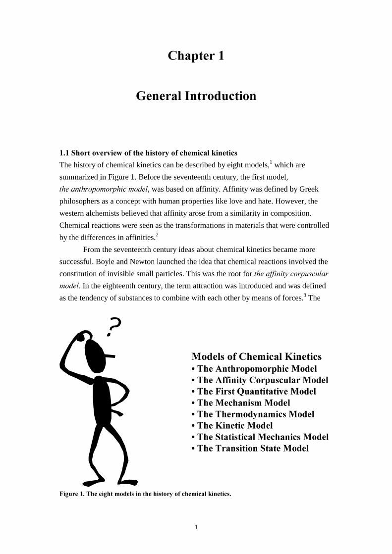
The history of chemical kinetics can be described by eight models,1 which are

summarized in Figure 1. Before the seventeenth century, the first model,

�� , was based on affinity. Affinity was defined by Greek

philosophers as a concept with human properties like love and hate. However, the

western alchemists believed that affinity arose from a similarity in composition.

Chemical reactions were seen as the transformations in materials that were controlled

by the differences in affinities.2

From the seventeenth century ideas about chemical kinetics became more

successful. Boyle and Newton launched the idea that chemical reactions involved the

constitution of invisible small particles. This was the root for ��

� ��. In the eighteenth century, the term attraction was introduced and was defined

as the tendency of substances to combine with each other by means of forces.3 The

�� !��"��

!�#��#��

��

2

rate of transformation was related to different degrees of affinity/attraction between

the particles. Bergman showed for the very first time in history that an increase of the

reaction temperature could change the affinities of the substances.4 Also ideas about

catalysts were developed. �� was the first model

concerned with the occurrence and the rate of chemical reactions. Predictions of the

occurrence and rates were very limited. They were based on affinity tables which were

empirically developed. A large drawback of the model was the absence of any

mathematical treatment between the energy of a system and the reaction rate.

The use of mathematics in chemical kinetics began in Germany in 1850 with

the quantitative investigation of the inversion of sucrose by Wilhelmy5 resulting in

�� . He produced the first quantitative rate law for chemical

reactions. He also introduced that a chemical reaction was a process in which particles

interacted and affinity was not playing a role at all.

Harcourt and Esson introduced �� in the nineteenth

century. The idea that in a chemical reaction particles interact with each other in

distinct steps was born.6 Esson developed empirical equations in which the amount of

product formed and time were connected. This resulted in integrated differential

equations for rates of chemical reactions. This was achieved for what we now call first

order, second order and pseudo-first order reactions. By means of the introduction of

mathematics in chemistry more accurate predictions of rates of chemical reactions

became available. Harcourt and Esson studied also the influence of temperature on

reaction rates in more detail. Within �� , Ostwald7 investigated the

catalysis within chemical reactions. He proposed the existence of alternative pathways

in catalyzed reactions. When at the beginning of the twentieth century it became

possible to detect and identify reaction intermediates using experimental techniques,

catalysis was developed further.

A large step forward in the study of chemical kinetics was achieved by

introduction of �� . Van ‘t Hoff8 investigated the energy

necessary for the occurrence of forward and backwards reactions in equilibrium

reactions. Arrhenius9 proposed that there is a minimum amount of energy necessary

for the reaction to occur which was defined as the energy barrier. Later, the term

activation energy was introduced. A key issue in �� is that a

relationship was introduced between energy and energy barrier, which was not present

in previous models.

In the twentieth century �� was introduced in which a new

attribute was defined. A chemical reaction, involving the breaking and making of

bonds, would be the cause of collisions between molecules.10 This led to the

introduction of a steric factor into the Arrhenius equation in order to explain why only

��

3

a proportion of the collisions occurring were effective. However, obtaining a

magnitude of the steric factor was very problematic.11 Despite these difficulties,

�� contributed to a better understanding of the process of a chemical

reaction and of the reasons why different reactions took place at different rates.

At the same time that �� was developed, a group of scientists

applied statistical mechanics to systems of reacting molecules resulting in

�� . Mathematical equations were derived for the rate of a

chemical reaction obtained from the consideration of the passage of systems through

the potential energy surface.12 Also the idea that radicals might be present in chemical

reactions was born.13

�� was a serious attempt in order to overcome the

shortcomings of all previous models discussed. The new model proposed that only

some of the molecules create transitional complexes. It became possible to derive the

concentration at which substances pass through the critical configuration of the

transition state by applying statistical methods. The model took into account the

statistical properties of reactive systems as well as the microscopic details of

molecular collisions.14,15 With the development of experimental techniques to detect

reaction intermediates a significant progress in the detailed understanding of the

mechanisms of catalyzed reactions became possible. Some important experimental

techniques are described in the next Section of this Chapter.

Nowadays, investigating rates of chemical reactions is a very popular topic.16

If reaction rates are known it is possible to estimate when a reaction mixture

approaches equilibrium, for example. Another reason for studying reaction rates is

that reaction mechanisms can be unraveled into elementary steps. Rates of chemical

reactions are also investigated to determine the end point of a reaction in process

industry. If rapid on-line estimation methods for reaction rate constants become

available then reaction rate constants of a certain chemical process can be monitored

on-line in order to control the process within the desired specification limits.

However, this is not applied yet and has to be developed still. This thesis can be seen

as a first step in this direction, because it reports applications of novel techniques

which are very suitable for rapid estimation of reaction rate constants.

�$�%&��'��

The first step in kinetic analysis is to obtain the concentrations of the reactants and

products at different times after the reaction has been initiated. The temperature must

be kept constant during the reaction which requires certain demands on the

experimental set-up, because most chemical reactions are sensitive to the temperature.

��

4

A procedure to obtain concentrations of chemical species in time of a reacting

system is the following. Samples of the reaction mixture are taken in time by means of

the quenching method.16 In the quenching method samples are cooled suddenly or

added to a large amount of solvent which will stop the reaction. Subsequently, the

quenched samples are analyzed using techniques like: titration, mass spectrometry,

gas chromatography, polarimetry, nuclear magnetic resonance or spectroscopy, for

example, in order to obtain concentrations of different species involved in the reacting

system. If concentrations of different species in the reaction mixture are obtained in

time, a kinetic model can be fitted to the concentration versus time data. This results

in an estimation of the unknown reaction rate constants.17-19

The quenching procedure has some serious drawbacks. It is only applicable to

reactions that are quite slow. No reaction must occur during the time it takes to

quench the samples. Secondly, taking samples from the reaction mixture and

analyzing these samples is expensive and very time-consuming.

A reaction in which at least one species is a gas results in a change of pressure

in a system of constant volume. Hence, its progress can be followed by measuring the

pressure difference in time. A disadvantage of the method is that it is far from

specific, because all gas-phase species contribute to the pressure differences

measured.

The use of on-line spectroscopic techniques overcomes the shortcomings of

the quenching procedure discussed as shown in this thesis. On-line spectroscopic

techniques are explained in the next Section of this Chapter.

�(��

Using spectroscopic techniques, for example infrared (IR) spectroscopy,20,21 it is

possible to monitor specific reacting IR absorbing species of chemical reactions

without the need to take samples of the reacting system. Spectroscopic monitoring of

reactions can be realized by using probes, flowcells and optical fibers. In the

fingerprint area of IR, bands of functional groups are sharp. A disadvantage of IR

spectroscopy is that very short light pathlengths (µm’s) are required, which makes the

measurements more difficult.

Nowadays, a lot of commercial software packages are available for estimating

reaction rate constants from spectral data like KINSIM22 and FITSIM.23 However,

these packages can only deal with univariate progress curves. The absorption spectra

that are characteristic for spectroscopic techniques contain wide bands that might have

a large spectral overlap. In such complex spectra it is difficult to find single

wavelengths that are specific for only one of the reacting absorbing species. For

wavelengths that are not specific for only one reacting absorbing species the molar

��

5

absorbances of the individual reacting absorbing species have to be known. Hence, in

reasonably complex cases methods like KINSIM and FITSIM fail. Multivariate

analysis tools can overcome the mentioned problems as is shown in this thesis.

Using near-infrared (NIR) spectroscopy, short-wavelength near-infrared

(SW-NIR) spectroscopy or UV-Vis spectroscopy20,21 it is possible to use longer light

pathlengths (mm’s - cm’s), making the experimental set-up easier and more widely

applicable. Several publications have shown applications of SW-NIR spectroscopy to

monitor processes. Cavinato ��.24 used SW-NIR for the determination of ethanol

during the time course of a fermentation process. The measurements were performed

non-invasively. Aldridge��.25 used SW-NIR to monitor the free radical

polymerization of methyl-methacrylate. The conversion was obtained by a plot of one

specific wavelength, representative for the monomer, of the recorded spectra versus

reaction time. The reaction rate constants of the chemical reactions studied were not

estimated in the publications mentioned in this paragraph.

In 1974, Sylvestre ��26 published a paper which describes the first

application of spectroscopic techniques to estimate reaction rate constants from

chemical reactions using multivariate analysis tools. In the literature, there are a lot of

papers published on this topic.27-34 In these publications the emphasis is not on the

spectroscopic techniques used, but there is focussed on new multivariate approaches

to estimate the reaction rate constants from the spectral data obtained. Important

multivariate analysis tools are discussed in the next Section of this Chapter. In this

thesis, new multivariate analysis tools are presented.

�)��

Chemometrics is a part of chemistry that develops mathematical and statistical

methods for analyzing chemical data.35 Multivariate analysis is widely used in

chemometrics. Curve resolution36 is a group of multivariate analysis tools based on

the determination of qualitative information and the recovery of response profiles, for

example time profiles. Nowadays, new modifications of curve resolution techniques

and applications have been published.37-44

The traditional curve resolution techniques can be adapted in order to estimate

pure spectra of reacting absorbing species and reaction rate constants simultaneously

from spectral data of the reacting system using specific kinetic model information as

is shown in this thesis. In that case, equations describing the kinetics are used

explicitly by the algorithm.26-34 In the curve resolution methods, an iterative least

squares optimization procedure is implemented to estimate the values of the unknown

parameters. The pure spectra obtained can be used to identify chemical species using

��

6

library spectra. This is useful for checking the reaction mechanism and locating

unknown side reactions.

For processes with unknown stoichiometry, curve resolution can be combined

with target factor analysis (TFA).45,46 The Kalman filter is also a very popular tool for

estimating reaction rate constants from spectroscopic data.47,48 Otto gives a short

overview of the use of multivariate analysis tools in kinetic analysis.49 The use of

three-way analysis to estimate reaction rate constants from batch processes is a new

approach.50,51 In that approach different kinetic runs are analyzed simultaneously if

these several runs have a certain correlation in the data structure. In a specific case it

is possible to create a three-way structure from only one spectral dataset as is shown in

this thesis.

�*��

The accuracy of reaction rate constant estimates can possibly be improved by using

constraints during the optimization procedure. In the literature, constraints like

unimodality of concentration profiles,52,53 closure,51,52 selectivity52 and non-negativity

of both concentration profiles and pure spectra51,52 are used as constraints during

optimization of the curve resolution model in order to improve the accuracy of

parameter estimates. Often some of the pure spectra of the absorbing species involved

in the chemical reactions of interest are known beforehand or easy to measure. This

information can be implemented in adapted curve resolution methods as is shown in

this thesis. In three-way analysis constraints are very often used to avoid numerical

problems and to speed up the algorithms.51,54,55 Constraints in three-way analysis are

also discussed in this thesis.

�+��

The initial aim of the work described in this thesis was to use and adapt existing curve

resolution based methods to estimate reaction rate constants from spectroscopic data

obtained in time of chemical reactions, to validate the obtained parameter estimates

and to investigate the use of constraints within curve resolution methods. When

Antalek and Windig56 published a paper about the use of non-iterative three-way

methods for estimating parameters from exponential profiles, it became a challenge to

modify and apply these methods to kinetic profiles. This has been investigated in

detail and new iterative three-way methods, specific for estimating reaction rate

constants, have been developed. This thesis gives an overview of the theory of several

two-way and three-way methods. Applications of these methods to simulated and

experimental data are reported.

��

7

�,��

This thesis is organized as follows. In ��$, the measurement model is

explained in detail and the theory of some two-way methods is presented. Also

attention is paid to the use of constraints within these methods. In ��(, the

three-way methods are presented. Also in this Chapter the use of constraints is

discussed. In ��), methods in order to achieve quality assessment of obtained

reaction rate constant estimates are reported. ��*, deals with a detailed

overview of four experimental datasets used in this thesis. A short summary of the

datasets can be found in the Appendix. Applications of two-way methods and

three-way methods to simulated and experimental data are given in ��+ and ,,

respectively. ��- treats the comparison between the performance of two-way

and three-way methods. ��. is concerned with the implementation of

constraints within a specific curve resolution method, discussed in ��$.

General conclusions of the work presented and suggestions for further research are

given in ��/.

The methods presented in this thesis are not applied to all datasets which are

described in ��*. This is because of the large time gap between the

measurements of several datasets. This thesis is organized in such a way, that

�� +, ,, - and ., which all deal with applications, can be read independently.

This also holds for ��$, (, ) and *, which deal with theory and the description

of experimental datasets. However, all �� use the measurement model defined

in ��$, ��$�$.

�-�0��1. Justi R, Gilbert JK. ‘History and philosophy of science through models: The case of chemical

kinetics’. �� , 1999; -: 287-307.

2. Mellor JW. �� , Longmans Green: London, 1904.

3. Duncan A. �� !� ��"��#��, Oxford University Press: Oxford,

1996.

4. Mierzecki R. ��$��, Kluwer: Dordrecht, 1991.

5. Farber E. ‘Early studies concerning time in chemical reactions’. ��, 1961; ,: 875-894.

6. Partington JR. %�$��&'��(), MacMillan: London, 1964.

7. Ostwald W. �� *��, Longman Green: New York, 1909.

8. Van ‘t Hoff JH. �� , Frederick Miller and Williams & Norgate:

Amsterdam and London, 1896.

9. Arrhenius S. ‘On the reaction velocity of the inversion of cane sugar by acids’, in �� +�� "�

��,��, ed. By Black MH, Laidler KJ. Pergamon Press: Oxford, 1967;

31-35.

10. Glasstone S, Laidler KJ, Eyring H. ��+��*��#��,��

+��-�'��-�� , Erlbaum: New Jersey, 1941; 3-34.

��

8

11. Rice OK, Ramsberger HC. ‘Theories of unimolecular reactions at low pressures’. .��%��

��, 1927; ).: 1617.

12. Semenoff N. ‘The oxidation of phosphorus vapour at low pressures’, in �� +�� "��

��,��, ed. By Black MH, Laidler KJ. Pergamon Press: Oxford, 1967; 127-153.

13. Christiansen JA. ‘On the reaction between hydrogen and bromine’, in �� +�� "��

��,��, ed. By Black MH, Laidler KJ. Pergamon Press: Oxford, 1967; 119-126.

14. Evans MG, Polanyi M. ‘Some applications of the transition state method to the calculation of

reaction velocities’. ��/�� , 1935; (: 875-894.

15. Evans MG. ‘Thermodynamical treatment of transition state’. ��/�� ,

1938; (): 49-57.

16. Atkins PW. *��, Oxford University Press: Oxford, 1998, Chapter 25.

17. Kaufman D, Sterner C, Masek B, Svenningsen R, Samuelson G. ‘An NMR kinetics experiment’.

.�� , 1982; *.: 885-886.

18. Chrastil J. ‘Determination of the first order consecutive reaction rate constants from final product’.

��, 1988; $: 289-292.

19. Chrastil J. ‘Determination of the first-order consecutive reversible reaction kinetics’. ��,

1993; ,: 103-106.

20. Burns DA, Ciurczak EW. $�� 0��1��#�� %��, Dekker: New York, 1992.

21. Workman JR JJ. ‘Interpretive spectroscopy for near infrared’.�%��+�� , 1996; (:

251-320.

22. Barshop BA, Wrenn RF, Frieden C. ‘Analysis of numerical methods for computer simulation of kinetic

processes: Development of KINSIM-A flexible, portable system’. %��2��, 1983; (/:

134-145.

23. Zimmerle CT, Frieden C. ’Analysis of progress curves by simulations generated by numerical

integration’. 2��.�, 1989; $*-: 381-387.

24. Cavinato AG, Mayes DM, Ge Z, Callis JB. ‘Noninvasive method for monitoring ethanol in

fermentation processes using fiber-optic near-infrared spectroscopy’. %��, 1990; +$:

1977-1982.

25. Aldridge PK, Burns DH, Kelly JJ, Callis JB. ‘Monitoring of methylmethacrylate polymerization

using non-invasive SW-NIR spectroscopy’.�*�� 3��, 1993; ): 155-160.

26. Sylvestre EA, Lawton WH, Maggio MS. ‘Curve resolution using a postulated chemical reaction’.

��, 1974; +: 353-368.

27. Mayes DM, Kelly JJ, Callis JB. ‘Non-invasive monitoring of a two-step sequential chemical reaction

with shortwave near-infrared spectroscopy’, in 1��#+� ��4�2�� "��"��

0�� %�� 1�+�%��, ed. by Hildrum KI, Isaksson T, Naes T, Tandberg A.

Ellis Horwood: Chichester, 1992; 377-387.

28. Chau F-T, Mok K-W. ‘Multiwavelength analysis for a first-order consecutive reaction’. ��

��, 1992; +: 239-242.

29. Bugnon P, Chottard J-C, Jestin J-L, Jung B, Laurenczy G, Maeder M, Merbach AE, Zuberbühler AD.

‘Second-order globalisation for the determination of activation parameters in kinetics’. %��

%��, 1994; $.-: 193-201.

30. Tam KY, Chau FT. ‘Multivariate study of kinetic data for a two-step consecutive reaction using target

factor analysis’. ��0��, 1994; $*: 25-42.

31. Maeder M, Molloy KJ, Schumacher MM. ‘Analysis of non-isothermal kinetic measurements’. %��

��%��, 1997; ((,: 73-81.

��

9

32. Furusjö E, Danielsson L-G. ‘A method for the determination of reaction mechanisms and rate constants

from two-way spectroscopic data’. %��%��, 1998; (,(: 83-94.

33. Molloy KJ, Maeder M, Schumacher MM. ‘Hard modelling of spectroscopic measurements.

Applications in non-ideal industrial reaction systems’. ��0��, 1999; )+:

221-230.

34. Furusjö E, Danielsson L-G. ‘Target testing procedure for determining chemical kinetics from

spectroscopic data with absorption shifts and baseline drift’. ��0��, 2000;

*/: 63-73.

35. Massart DL, Vandeginste BGM, Buydens LMC, de Jong S, Lewi PJ, Smeyers-Verbeke J.

$�� 0�� 3��, Elsevier: Amsterdam, 1997.

36. Lawton WH, Sylvestre EA. ‘Self modeling curve resolution’. ��, 1971; (: 617-633.

37. Shrager RI, Hendler RW. ‘Titration of individual components in a mixture with resolution of difference

spectra, pK’s, and redox transitions’. %��, 1982; *): 1147-1152.

38. Frans SD, Harris JM. ‘Reiterative least-squares spectral resolution of organic acid/base mixtures’.

%��, 1984; *+: 466-470.

39. Frans SD, Harris JM. ‘Least squares singular value decomposition for the resolution of pK’s and

spectra from organic acid/base mixtures’. %��, 1985; *,: 1718-1721.

40. Shrager RI. ‘Chemical transitions measured by spectra and resolved using singular value

decomposition’. ��0��, 1986; : 59-70.

41. Tauler R, Fleming S, Kowalski BR. ‘Multivariate curve resolution applied to spectral data from

multiple runs of an industrial process’. %��, 1993; +*: 2040-2047.

42. Lacorte S, Barceló D, Tauler R. ‘Determination of traces of herbicide mixtures in water by on-line

solid-phase extraction followed by liquid chromatography with diode-array detection and multivariate

self-modelling curve resolution’. .��"��%, 1995; +.,: 345-355.

43. Tauler R, Izquierdo-Ridorsa A, Gargallo R, Casassas E. ‘Application of a new multivariate curve

resolution procedure to the simultaneous analysis of several spectroscopic titrations of the

copper (II)-polyinosinic acid system’. ��0��, 1995; $,: 163-174.

44. Casassas E, Marqués I, Tauler R. ‘Study of acid-base properties of fulvic acids using fluorescence

spectrometry and multivariate curve resolution methods’. %��%��, 1995; (/: 473-484.

45. Bonvin D, Rippin DWT. ‘Target factor analysis for the identification of stochiometric models’.

��"��, 1990; )*: 3417-3426.

46. Harmon JL, Duboc Ph, Bonvin D. ‘Factor analytical modeling of biochemical data’. ��

��"�, 1995; .: 1287-1300.

47. Jimenez-Prieto R, Velasco A, Silva M, Perez-Bendito D. ‘Kalman filtering of data from first- and

second-order kinetics’. ��, 1993; )/: 1731-1739.

48. Mok K-W, Chau F-T. ‘Application of the extended Kalman filter for analysis of a consecutive

first-order reaction’. �� %��, 1996; *: 170-174.

49. Otto M. ‘Chemometrics in kinetic analysis’. ��%��, 1990; *: 685-688.

50. Gui M, Rutan SC, Agbodjan A. ‘Kinetic detection of overlapped amino acids in thin-layer

chromatography with a direct trilinear decomposition method’. %��, 1995; +,: 3293-3299.

51. Saurina J, Hernandez-Cassou S, Tauler R. ‘Multivariate curve resolution and trilinear

decomposition methods in the analysis of stopped-flow kinetic data for binary amino acid mixtures’.

%��, 1997: +.: 2329-2336.

52. Tauler R, Smilde A, Kowalski B. ‘Selectivity, local rank, three-way data analysis and ambiguity in

multivariate curve resolution’. .��, 1995; .: 31-58.

��

10

53. de Juan A, van der Heyden Y, Tauler R, Massart, DL. ‘Assessment of new constraints applied to the

alternating least squares method’. %��%��, 1997; ()+: 307-318.

54. Saurina J, Hernandez-Cassou S., Tauler R. ‘Multivariate curve resolution applied to

continuous-flow spectrophotometric titrations. Reaction between amino acids and

1,2-naphthoquinone-4-sulfonic acid’ %��, 1995; +,: 3722-3726.

55. Bro R. 5��#6��%��/�� 4�5� ��-�%�"�� %��, Doctoral

Thesis, 1998.

56. Antalek B, Windig W. ‘Generalized rank annihilation method applied to a single multicomponent

pulsed gradient spin echo NMR data set’. .��%��, 1996; -: 10331-10332.

11

��

��

��

The theory of the two-way methods traditional curve fitting (TCF), classical curve

resolution (CCR) and weighted curve resolution (WCR) for estimating reaction rate

constants from spectroscopic data in time of chemical reactions is described in this

Chapter. Constraints that can be implemented into these two-way methods are also

discussed. Before algorithms and the implementation of constraints are treated in

detail, the measurement model is described firstly.

��

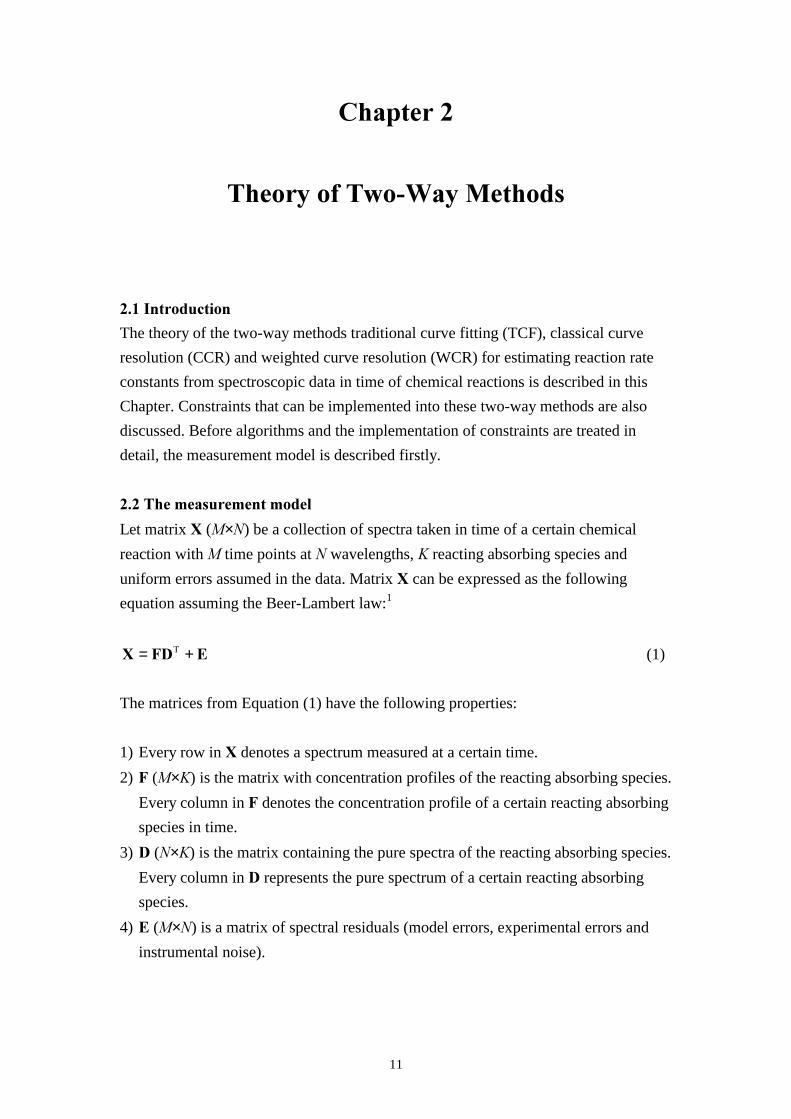
Let matrix � (�×�) be a collection of spectra taken in time of a certain chemical

reaction with � time points at � wavelengths, � reacting absorbing species and

uniform errors assumed in the data. Matrix � can be expressed as the following

equation assuming the Beer-Lambert law:1

�� += T (1)

The matrices from Equation (1) have the following properties:

1) Every row in � denotes a spectrum measured at a certain time.

2) � (�×�) is the matrix with concentration profiles of the reacting absorbing species.

Every column in � denotes the concentration profile of a certain reacting absorbing

species in time.

3) (�×�) is the matrix containing the pure spectra of the reacting absorbing species.

Every column in represents the pure spectrum of a certain reacting absorbing

species.

4) � (�×�) is a matrix of spectral residuals (model errors, experimental errors and

instrumental noise).

��

12

Suppose the following two-step consecutive reaction is considered with

second order reaction rate constant a (M-1min-1) and first order reaction rate constant

2 (min-1).

�� NND →→+ 2

Equation (2)-(5) describe the differential equations of species �, �, � and �,

respectively.

� ��

� �D

[ ][ ][ ]= − (2)

� ��

� ��

[ ] [ ]= (3)

][]][[][

2 � ��

D−= (4)

][][

2 � �� = (5)

The first reaction step of the two-step consecutive reaction can be made pseudo-first

order if reactant � is present in large excess. In that case, the reaction can be described

as:

�� NN →→ 21

with pseudo-first order reaction rate constant 1 (min-1). If the first reaction step is a

pseudo-first order reaction, Equation (6)-(8) can be used to describe the concentration

profiles of species �, � and �, respectively.

� � 8 L 8

N WL

, ,= −0

1 (6)

)( 21

12

10,,

LLWNWN8

L:

�� −− −

−= (7)

� � � �< L 8 8 L : L, , , ,= − −0 (8)

��

13

where �8�� is the initial concentration of �; �8�L��:�L�and��<�L� are the concentrations

of �, � and � at time tL, respectively. It is assumed that only species � and species �

are present at the start of the reaction. The relation given in Equation (9) links the

second order reaction rate constant a and the pseudo-first order reaction rate constant

1 discussed.

0

1

][�

D

= (9)

where [�]0 is the initial concentration of species �.

If concentrations in time of the reacting absorbing species are available, the

reaction rate constants can be obtained by fitting, for example, Equation (6)-(8) in

case of pseudo-first order conditions to the time versus concentration data using

mathematical techniques.2-4 However, in practice only � is �� and � and are

both �� . In that case, it is impossible to estimate the reaction rate constants of

the considered chemical reaction using techniques which are based on fitting the

kinetic expressions to the concentration versus time data since these concentrations

are not measured. Often, it is possible to obtain a part of by means of measuring

pure spectra of reactants and products. However, obtaining pure spectra of

intermediate species can be a problem because they are difficult to isolate. Matrix � is

�� , but a model for � (structure) is �� if a suitable kinetic model for the

chemical reaction of interest and the initial concentrations of the different reacting

absorbing species are ��. Iterative algorithms are necessary in order to estimate

the reaction rate constants of interest. Three iterative algorithms which can be used to

achieve this goal are described in Sections 2.3, 2.5 and 2.6 of this Chapter. In the next

Sections it is assumed that species �, � and � are spectroscopically active whereas

species � is not spectroscopically active.

�!��"�� #

In traditional curve fitting (TCF) reaction rate constants are estimated from the

absorbance differences in time, which is a concentration profile of a certain species,

obtained from one (or more) selective wavelength(s), that is (are) specific for mainly

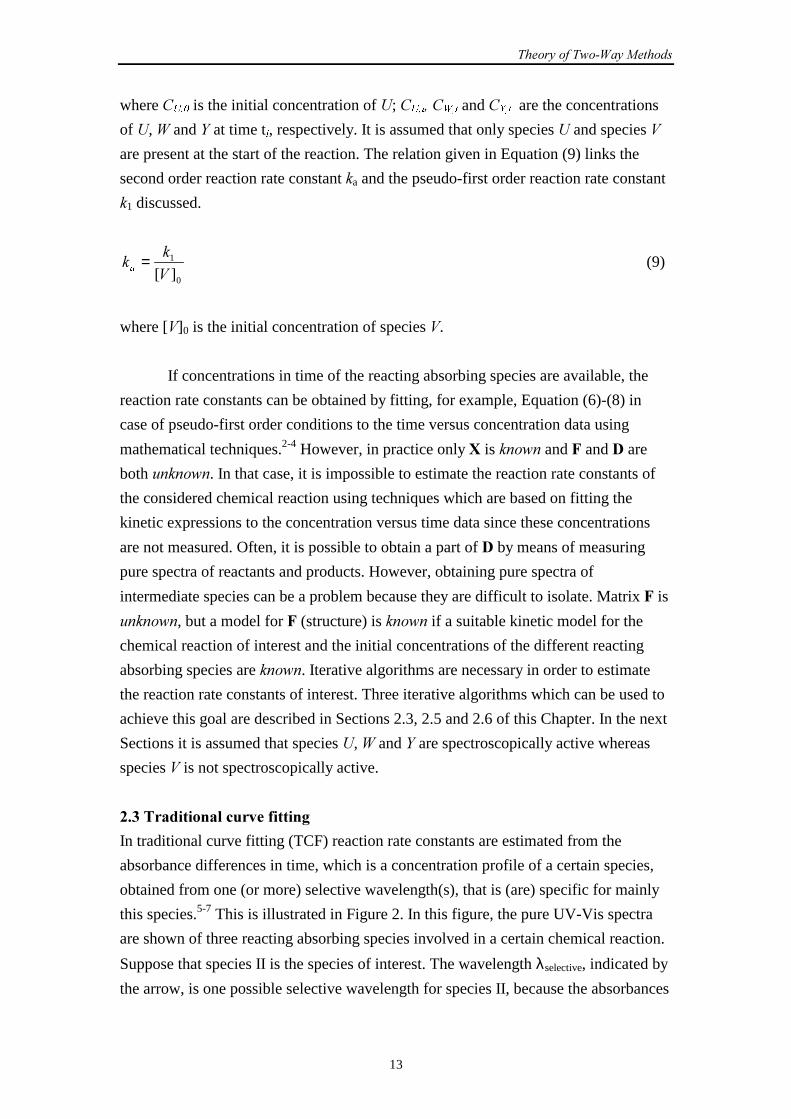
this species.5-7 This is illustrated in Figure 2. In this figure, the pure UV-Vis spectra

are shown of three reacting absorbing species involved in a certain chemical reaction.

Suppose that species II is the species of interest. The wavelength λselective, indicated by

the arrow, is one possible selective wavelength for species II, because the absorbances

��

14

!$$ !%$ !&$ %$ %'$ ($$$

$�%

$�&

��

��"��#��)��*

+,��,��)+�-�*

λselective

�T

λselective.��.��

��

�

��

��

/��0��

��/��

+,��,��

��

��#��"�� #�

of species I and III at this wavelength are very small. From the absorbance versus time

data obtained from one or more selective wavelengths, which results in a

concentration profile, unknown reaction rate constants can be estimated quite easily

and fast. This is done by means of fitting the rate equation of the specific species to

the obtained concentration profile. It is important to stress that TCF is an univariate

method in case of one selective wavelength.

Consider the measurement model described in Section 2.2 of this Chapter.

From Equation (4) in case of second order kinetics or from Equation (7) in case of

pseudo-first order kinetics, it is observed that the reaction rate constants of interest,

a and 2 or 1 and 2, can be estimated from �� the concentration profile of the

intermediate species (species �). Hence, if one or more selective wavelengths are

chosen for the intermediate species, the reaction rate constants can be estimated from

the concentration profile obtained from the absorbance versus time data. Selective

wavelengths for the intermediate species can be obtained using fixed-size window

evolving factor analysis (FSWEFA), a local rank selection method.8-10 Also other

local rank selection methods like heuristic evolving latent projection (HELP)11,12

could be used to obtain these selective wavelengths. In FSWEFA selective

��

15

wavelengths are obtained from a matrix containing the spectra of the reacting system

in time. The FSWEFA technique is explained in more detail in the next Section.

After selective wavelengths have been obtained, the mean absorbance for the

selective wavelengths chosen for every time point is calculated. This will give a

concentration profile for the intermediate species. It is essential that the pure spectra

of reactant and product are both known in advance. Finally, the concentration profile

obtained is fitted to the equation of the theoretical concentration profile of the

intermediate species using the Levenberg-Marquardt algorithm.13 This algorithm, for

finding an optimum in a response surface, smoothly varies between two methods for

finding the optimum, the steepest decent method, that is used �� from the optimum,

and the inverse Hessian method, that is used �� to the optimum.

�%��1��2��"��"��#� ��

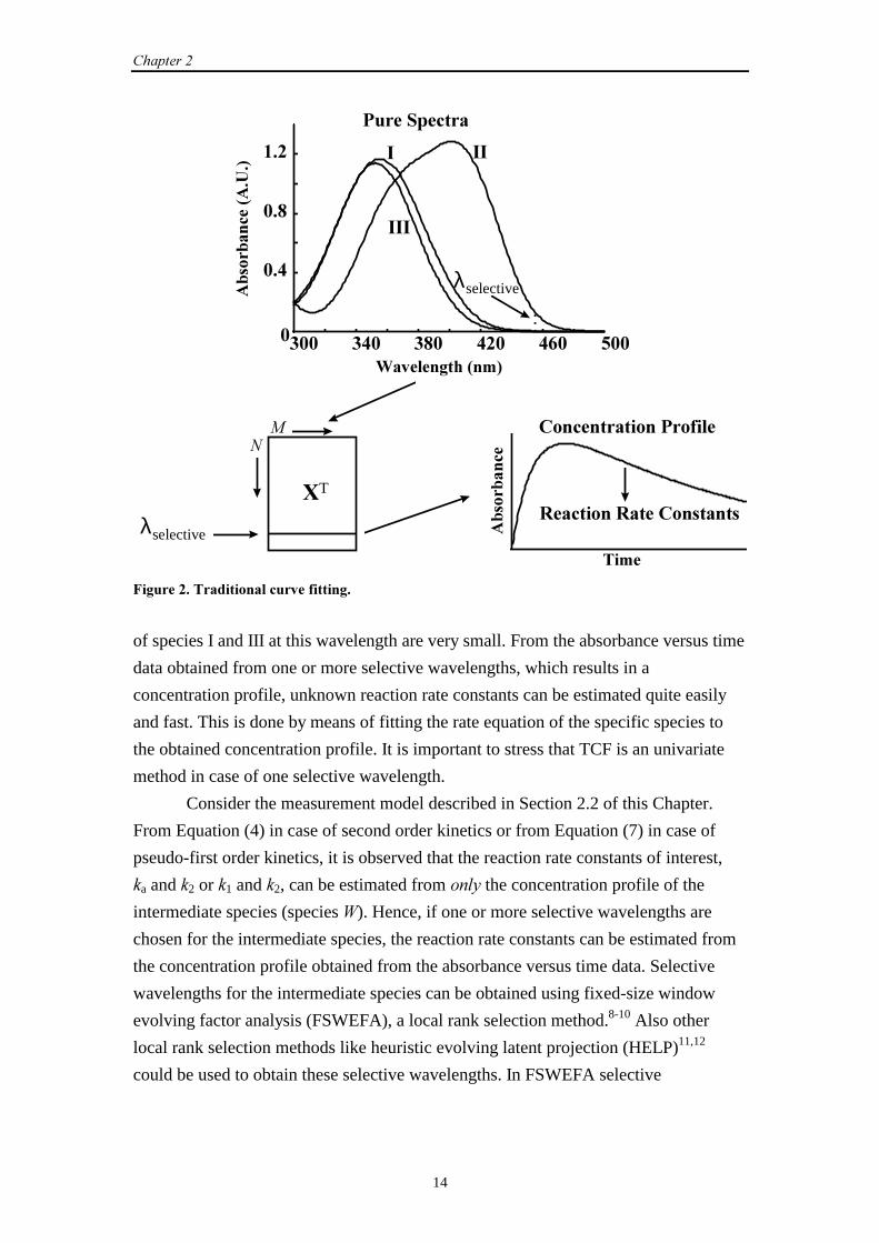
Fixed size window evolving factor analysis (FSWEFA)8-10 is applicable if the rows or

columns of a matrix have a certain structure, for example the appearance and

disappearance of chemical species in time. In FSWEFA a window of rows or columns

is selected which is moved over the dataset. Typically a window size equal to the

number of expected reacting absorbing chemical species, for example, is chosen. At

each position of the window a singular value decomposition (SVD)14 is calculated and

the associated singular values are plotted as a function of the position of the window.

In this way, local rank can be estimated. This procedure is illustrated in Figure 3.

�T�

�

�T��

�T��

�T��

��

03 03 03

3RVLWLRQ�RI�WKH�ZLQGRZ

ORJ��VLQJXODU�YDOXH�

4��5�6��

��"��#�� "��#��

��#��!��1��2��"��"��#� ��)�0��+*�

��

16

In this thesis, FSWEFA has been applied in the spectral domain, because

selective wavelengths have to be located. Therefore, a fixed size window of three

wavelengths has been moved over the rows of datamatrix �T, because it is known that

three reacting absorbing species are involved in the reacting system in case of the

reaction described in Section 2.2 of this Chapter. However, in Figure 3, a fixed size

window of ten wavelengths has been moved over the rows of �T. From the plots of

the log (singular value) versus position of the window, local rank of one, representing

the presence of mainly the intermediate, is detected. From these plots it is obvious that

three reacting absorbing species are involved and hence it is sufficient to use a fixed

window size of three wavelengths instead of ten wavelengths. The approach presented

can only be applied, if the pure spectra of reactant and product are both known in

advance. The pure spectrum of reactant and product are both shown in Figure 2 of the

previous Section indicated by species I and species III, respectively. Because the

position of the window corresponds to a certain sequence of three wavelengths,

selective wavelengths for the intermediate are obtained quite easily.

�(��"��

Curve resolution15,16 is a set of techniques based on the determination of qualitative

information and the recovery of response profiles, for example time profiles. If

parameters of interest, for example reaction rate constants, are incorporated as

unknowns in curve resolution this results in modifications of curve resolution

techniques, because specific kinetic information is used explicitly. One of these

modifications is the classical curve resolution (CCR) algorithm.17 In CCR, an estimate

for a and 2 in case of second order kinetics or an estimate of 1 and 2 in case of

pseudo-first order kinetics and an estimate of can be obtained simultaneously by

minimization of the sum of squares (SSQ) of residuals defined in Equation (10).

∑∑= =

=0

P

1

Q

PQ��

1 1

2 (10)

where the residual PQ is the !,�th element of matrix � from Equation (1).

The differential equations in case of second order kinetics are solved

numerically using the Runge-Kutta (4,5) formula.13 In that case, numerical integration

is part of the algorithm. Stepwise the algorithm works as follows according to an

alternating least squares scheme.

"�#�#��#$��#��

��

17

Construct the estimate of �, � , using Equation (2)-(5) in case of second order kinetics

or Equation (6)-(8) in case of pseudo-first order kinetics and the starting values for the

reaction rate constants.

�#�#!#$��#��

Repeat step 1 up to step 5 of the following minimization loop until the SSQ has been

minimized.

1) Minimize Equation (11) with respect to , where is obtained using

Equation (12) which represents an ordinary least squares step.

2T

ˆ

ˆˆmin ��'

− (11)

1TT )ˆˆ(ˆˆ −= �� (12)

2) Update the reaction rate constants using the Levenberg-Marquardt13 algorithm

according to Equation (13).

2T

ˆ,ˆ

ˆˆmin21

�� −NN

(13)

3) Calculate � , according to Equation (14).

Tˆˆˆ �� = (14)

4) Calculate matrix � by applying Equation (15).

�� ˆ−= (15)

5) Calculate SSQ.

It is important to stress that step 1 and step 2 reduce the sum of squares of

residuals and convergence is guaranteed. This is the principle of alternating least

squares. The columns of matrix � are �� updated simultaneously in %� iteration.

Hence, �� concentration profiles are updated simultaneously in %� iteration.

Moreover, only starting values for the reaction rate constants are required and no

��

18

initial estimates of the pure spectra are needed. In the Appendix a proof is given that

assuming the kinetic model proposed in this thesis is sufficient for uniqueness of the

solution of the curve resolution model and no rotational freedom of the solution is

present.

CCR can account for non-uniform errors present in the data by using weighted

least squares (WLS) if the structure of the measurement error is known.18 However,

the use of WLS is beyond the scope of this thesis, since the structure of this

measurement error is unknown.

�'��#��"��

Equation (16) shows the SVD of �T (�×�) assuming � ≤ �. For the cases where

�<� is valid � can be used instead of �T.

TT -03� = (16)

with -T- = �, 3T3 = 33T = �, - (�×�), 3 (�×�) and 0 (�×�) is a diagonal matrix

with the non-negative singular values arranged in decreasing order on the diagonal.

Equation (17) shows the truncated version of Equation (16) to the first & significant

singular values.

TTT or//////

-03��30-� == (17)

/- (�×&) contains the first & columns of - ,

/0 (&×&) is the upper left part of 0 ,

/3 (�×&) represents the first & columns of 3 , �-- =

//

T and �33 =//

T . The

estimate of �, �� , is reconstructed using the valid kinetic equations and the starting

values for the reaction rate constants. If Equation (1) from Section 2.2 holds then ��

and 3L span the same space and are connected with each other by means of a

transformation matrix 7 according to Equation (18).

7�3 ˆˆ=/

(18)

with

/3��7 T1T ˆ)ˆˆ(ˆ −= (19)

��

19

Following the target factor analysis (TFA) approach used by Maeder ��.19-21 the

objective function given in Equation (20) is minimized over 1 and 2 ensuring that for

the proper 1 and 2 the minimum of zero will be attained.

2

ˆ,ˆ)ˆˆ(min

21

//

NN

07��3 (20)

where 3/

and 0/ are both fixed during optimization. Because the columns of 3

/ are

weighted by 0/ in order to account for the differences in the order of magnitude of

importance of the different columns of 3/

as suggested by Shrager,22 the algorithm is

called weighted curve resolution (WCR). This approach can be very valuable in case

of data with a poor signal to noise ratio. If Equation (20) is used without weighting the

columns of 3/

, the algorithm is called curve resolution (CR) in this thesis.

From Equation (20) it is obvious that WCR reflects a separable problem,

because the concentration space and spectral space are separated. This is an important

difference between CCR and WCR. In WCR only reaction rate constant estimates are

obtained whereas in CCR reaction rate constant estimates and pure spectra estimates

are obtained simultaneously. In WCR, the matrix with concentration profiles, �� , can

be reconstructed using the optimal values of the reaction rate constants found. An

estimate of the pure spectra of the reacting absorbing species, , can be obtained by

applying Equation (12) from the previous Section.

If the reaction rate constants are estimated, the relative fit error can be

calculated according to Equation (21) and (22) for CR and WCR, respectively.

%100*ˆˆ

errorfitRelative/

/

3

7�3��

−= (21)

%100*)ˆˆ(

errorfitRelative//

//

03

07�3��

−= (22)

where a number of 0% indicates that there are no residuals left.

��

20

�8��

In Chapter 1, it has been explained already that the use of constraints implemented

into optimization algorithms can be very useful with respect to the accuracy of

reaction rate constant estimates. Three different types of constraints are considered in

this thesis. In ��#�� ' only the pure spectrum of the reactant is used in the

optimization procedure. In ��#��'( the pure spectra of reactant and product are

both used in the optimization procedure. In ��#��&� the pure spectra are

updated in each iteration of the optimization procedure using a non-negative least

squares step.23 Implementation of the three constraints mentioned in the optimization

procedure is only possible in case of CCR. In TCF and WCR, the pure spectra of

reacting absorbing species are not used during optimization of the reaction rate

constants and hence implementation of the constraints discussed is not possible. In the

next Chapter, the use of constraints within three-way methods is reported.

Using constraint R, the first column of matrix will be fixed during the

whole optimization procedure. Only the reaction rate constants and the pure spectra of

the intermediate and the product (second and third column of , respectively) are

updated simultaneously during the optimization procedure. Using constraint RP, the

first and third column of matrix will be fixed during the whole procedure. Only the

reaction rate constants and the pure spectrum of the intermediate (second column of

) are updated simultaneously during the optimization procedure. In the CCR

algorithm described in Section 2.5 the pure spectra are estimated using an ordinary

least squares step. In ��#��&� the pure spectra are updated in each iteration

using a non-negative least squares step.

�&�.� ��1. Burns DA, Ciurczak EW. )��*�� "��+��#�, Dekker: New York, 1992.

2. Kaufman D, Sterner C, Masek B, Svenningsen R, Samuelson G. ‘An NMR kinetics experiment’.

,-��!-�.��#��, 1982; (9: 885-886.

3. Chrastil J. ‘Determination of the first order consecutive reaction rate constants from final product’.

��!��-��!-, 1988; �: 289-292.

4. Chrastil J. ‘Determination of the first-order consecutive reversible reaction kinetics’. ��!��-��!-,

1993; �8: 103-106.

5. Drobnica L, Sturdik E. ‘The reaction of carbonyl cyanide phenylhydrazones with thiols’. /#��#!-

/#��-�+��, 1979; (&(: 462-476.

6. Bisby RH, Thomas EW. ‘Kinetic analysis by the method of nonlinear least squares’. ,-��!#��

.��#��, 1986; '!: 990-992.

7. Chau F-T, Mok K-W. ‘Multiwavelength analysis for a first-order consecutive reaction’. ��!��

��!-, 1992; �': 239-242.

8. Maeder M, Zuberbuehler AD. ‘The resolution of overlapping chromatographic peaks by evolving

factor analysis’. +��-��#!-�+��, 1986; �&�: 287-291.

��

21

9. Maeder M. ‘Evolving factor analysis for the resolution of overlapping chromatographic peaks’. +��-

��!-, 1987; (9: 527-530.

10. Keller HR, Massart DL. ‘Peak purity control in liquid chromatography with photodiode-array detection

by a fixed size moving window evolving factor analysis’. +��-��#!-�+��, 1991; %':

379-390.

11. Kvalheim OM, Liang Y-Z. ‘Heuristic evolving latent projections: Resolving two-way

multicomponent data. 1. Selectivity, latent-projective graph, datascope, local rank, and unique

resolution’. +��-��!-, 1992; '%: 936-946.

12. Liang Y-Z, Kvalheim OM, Keller HR, Massart DL, Kiechle P, Erni F. ‘Heuristic evolving latent

projections: Resolving two-way multicomponent data. 2. Detection and resolution of minor

constituents’. +��-��!-, 1992; '%: 946-953.

13. Press WH, Teukolsky SA, Vetterling WT, Flannery BP. ��!#��'�#��, Cambridge University

Press: New York, 1992.

14. Martens H., Naes T. ��#%�#��#*��#��, Wiley: Chichester, 1989.

15. Lawton WH, Sylvestre EA. ‘Self modeling curve resolution’. ��!�#��, 1971; �!: 617-633.

16. Sylvestre EA, Lawton WH, Maggio MS. ‘Curve resolution using a postulated chemical reaction’.

��!�#��, 1974; �': 353-368.

17. Frans SD, Harris JM. ‘Reiterative least-squares spectral resolution of organic acid/base mixtures’.

+��-��!-, 1984; (': 466-470.

18. Kiers HAL. ‘Weighted least squares fitting using ordinary least squares algorithms’, (��!�# �,

1997; ': 251-266.

19. Bugnon P, Chottard J-C, Jestin J-L, Jung B, Laurenczy G, Maeder M, Merbach AE, Zuberbühler AD.

‘Second-order globalisation for the determination of activation parameters in kinetics’. +��-��#!-

+��, 1994; 9&: 193-201.

20. Maeder M, Molloy KJ, Schumacher MM. ‘Analysis of non-isothermal kinetic measurements’. +��-

��#!-�+��, 1997; !!8: 73-81.

21. Molloy KJ, Maeder M, Schumacher MM. ‘Hard modelling of spectroscopic measurements.

Applications in non-ideal industrial reaction systems’. ��!�!�#��"��-�&�*-��-, 1999; %':

221-230.

22. Shrager RI. ‘Chemical transitions measured by spectra and resolved using singular value

decomposition’. ��!�!�#��"��-�&�*-��-, 1986; �: 59-70.

23. Bro R, de Jong S. ‘A fast non-negativity-constrained least squares algorithm’. ,-��!�!�#��, 1997;

��: 393-402.

��

22

23

��

��

��

In this Chapter, non-iterative and iterative three-way methods for estimating reaction

rate constants from spectroscopic data are described. It is possible to use constraints

within three-way methods. This is discussed in Section 3.7. Before the algorithms are

explained in detail the principle on which the three-way methods are based is

explained in the next Section.

��

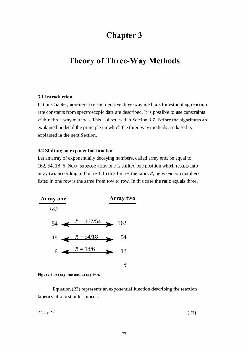
Let an array of exponentially decaying numbers, called array one, be equal to

162, 54, 18, 6. Next, suppose array one is shifted one position which results into

array two according to Figure 4. In this figure, the ratio, �, between two numbers

listed in one row is the same from row to row. In this case the ratio equals three.

��

��

54

18

6

��

162

54

18

�

��=�162/54

� = 54/18

��=�18/6

!��"��

Equation (23) represents an exponential function describing the reaction

kinetics of a first order process.

� � N W= − 1 (23)

��

24

where �1 is a reaction rate constant and � is the concentration of a certain species at

time . If the exponent is shifted in time, by means of introducing shift parameter �,

Equation (23) can be written as Equation (24).

� �V

N W 6= − +1( ) (24)

where �V is the “shifted concentration”. The ratio of Equation (23) and (24), called λis an indirect measure for �1 as is shown in Equation (25).

λ λ= = = = ⇒ =

−

− +− + +�

��

��

�V

N W

N W 6

N W N W 6 N 6

1

11 1 1

1( )( ) ln( )

(25)

Hence, the reaction rate constant �1 is calculated easily from the ratio of the

non-shifted and the shifted exponential function.

��

Consider the first reaction step, described in Section 2.2 of Chapter 2, under

pseudo-first order conditions. Equation (6) from Section 2.2 of Chapter 2, describes

the concentration profile of the reactant (species �). In this Section, it is supposed, for

convenience, that the initial concentration of species �, C8�0, is equal to 1 moll-1.

Assume that matrix # (�×�), as defined in Section 2.2 of Chapter 2, contains

spectroscopic measurements of only species � in time. This matrix contains two-way

data and no trilinear structure is present at first sight. However, it is possible to build a

trilinear structure according to the following procedure developed by Windig and

Antalek.1,2

Two matrices, #1 and #2, are created from # by means of a time shift �, which

can be any positive integer value between 1 and (�-1). This results in:

#1 = (#([1 . . . (�-�)])×�) and #2 = (#([(1+�) . . . �])×�). These two matrices

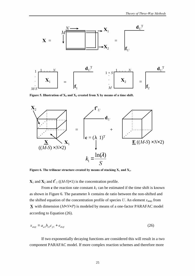
created by means of splitting # are visualized in Figure 5, where �8 (�×1) is the pure

spectrum of species �, 8 (�×1) is the concentration profile of species �,

1 ((�-�)×1) and 2 ((�-�)×1) are the concentration profiles of species � with time

shift � in matrices #1 and #2, respectively.

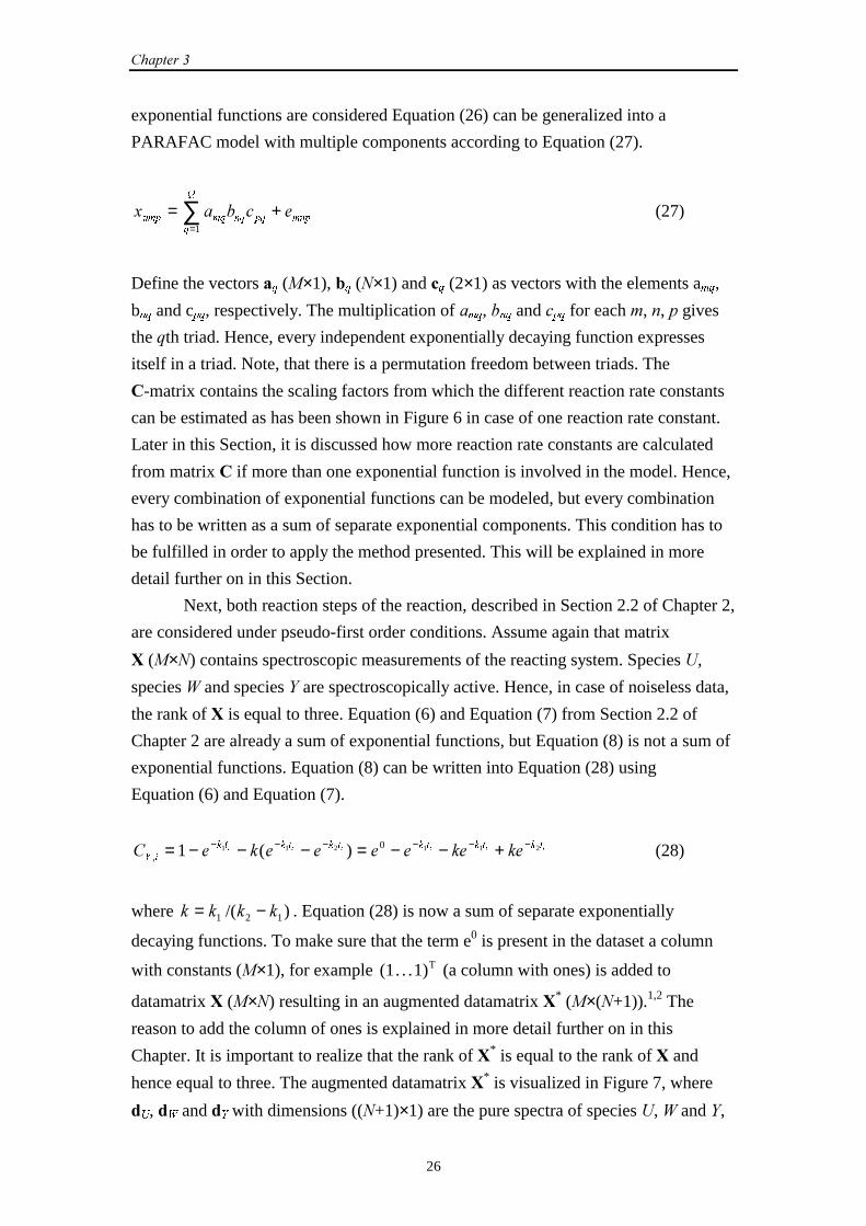
The matrices #1 and #2 formed by splitting # can be put into a trilinear or

PARAFAC3,4 model by means of stacking as shown in Figure 6 to construct a

three-way array # ((�-�)×�×2). Vector � (2×1) contains the scaling factors of

��

25

#1

1...

1 . . . �1 + �

�-�

.

.

.�

= = 1 2

�

# =

�

=

��T

�

#2

��T ��T

#1

#2

1 . . . �

!��$�� #��#�� %�#�&��%�� %��

= +

'�((�-�) ×�×2)

��

*�

((�-�) ×�×2)# #1

#2

��

)ln(1

λ=

� = ( 1)Tλ

!��(��&��%�� )��#��#��

#1 and #2 and *8 ((�-�)×1) is the concentration profile.

From � the reaction rate constant �1 can be estimated if the time shift is known

as shown in Figure 6. The parameter λ contains de ratio between the non-shifted and

the shifted equation of the concentration profile of species �. An element �PQS from

# with dimension (�×�×�) is modeled by means of a one-factor PARAFAC model

according to Equation (26).

PQSSQPPQS�� += 111 (26)

If two exponentially decaying functions are considered this will result in a two

component PARAFAC model. If more complex reaction schemes and therefore more

��

26

exponential functions are considered Equation (26) can be generalized into a

PARAFAC model with multiple components according to Equation (27).

� � � � �PQS PT QT ST PQS

T

4

= +=

∑1

(27)

Define the vectors �T (�×1), &T (�×1) and �T (2×1) as vectors with the elements aPT,

bQT and cST, respectively. The multiplication of �PT, �QT and �ST for each �, , gives

the !th triad. Hence, every independent exponentially decaying function expresses

itself in a triad. Note, that there is a permutation freedom between triads. The

�-matrix contains the scaling factors from which the different reaction rate constants

can be estimated as has been shown in Figure 6 in case of one reaction rate constant.

Later in this Section, it is discussed how more reaction rate constants are calculated

from matrix � if more than one exponential function is involved in the model. Hence,

every combination of exponential functions can be modeled, but every combination

has to be written as a sum of separate exponential components. This condition has to

be fulfilled in order to apply the method presented. This will be explained in more

detail further on in this Section.

Next, both reaction steps of the reaction, described in Section 2.2 of Chapter 2,

are considered under pseudo-first order conditions. Assume again that matrix

# (�×�) contains spectroscopic measurements of the reacting system. Species �,

species � and species " are spectroscopically active. Hence, in case of noiseless data,

the rank of # is equal to three. Equation (6) and Equation (7) from Section 2.2 of

Chapter 2 are already a sum of exponential functions, but Equation (8) is not a sum of

exponential functions. Equation (8) can be written into Equation (28) using

Equation (6) and Equation (7).

LLLLLLWNWNWNWNWNWN

L<�� 211211 0

, )(1 −−−−−− +−−=−−−= (28)

where )/( 121 �� −= . Equation (28) is now a sum of separate exponentially

decaying functions. To make sure that the term e0 is present in the dataset a column

with constants (�×1), for example T1) . . . (1 (a column with ones) is added to

datamatrix # (�×�) resulting in an augmented datamatrix #* (�×(�+1)).1,2 The

reason to add the column of ones is explained in more detail further on in this

Chapter. It is important to realize that the rank of #* is equal to the rank of # and

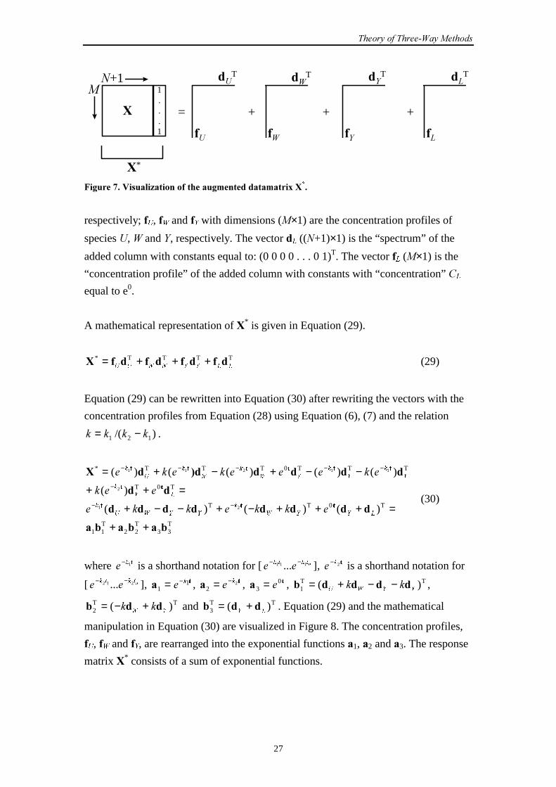
hence equal to three. The augmented datamatrix #* is visualized in Figure 7, where

�8, �: and �< with dimensions ((�+1)×1) are the pure spectra of species �, � and ",

��

27

= + +

�

��T ��T �"T

#

�+1

� "

+

�#T

#

� 1...1

#*

!��*��+��,�� %��%��# �

respectively; 8, : and < with dimensions (�×1) are the concentration profiles of

species �, � and ", respectively. The vector �/ ((�+1)×1) is the “spectrum” of the

added column with constants equal to: (0 0 0 0 . . . 0 1)T. The vector / (�×1) is the

“concentration profile” of the added column with constants with “concentration” �/

equal to e0.

A mathematical representation of #* is given in Equation (29).

TTTT*//<<::88� � � � # +++= (29)

Equation (29) can be rewritten into Equation (30) after rewriting the vectors with the

concentration profiles from Equation (28) using Equation (6), (7) and the relation

)/( 121 �� −= .

T33

T22

T11

T0TT

T0T

TTT0TTT*

)()()(

)(

)()()(()(

21

2

11211

&�&�&�

��

��

��-��#

WWW

WW

WWWWWW

++

=+++−+−−+

=++

−−+−+=

−−

−

−−−−−

/<<:

N

<<:8

N

/<

N

<

N

<

N

<:

N

:

N

8

N

��

��

��

(30)

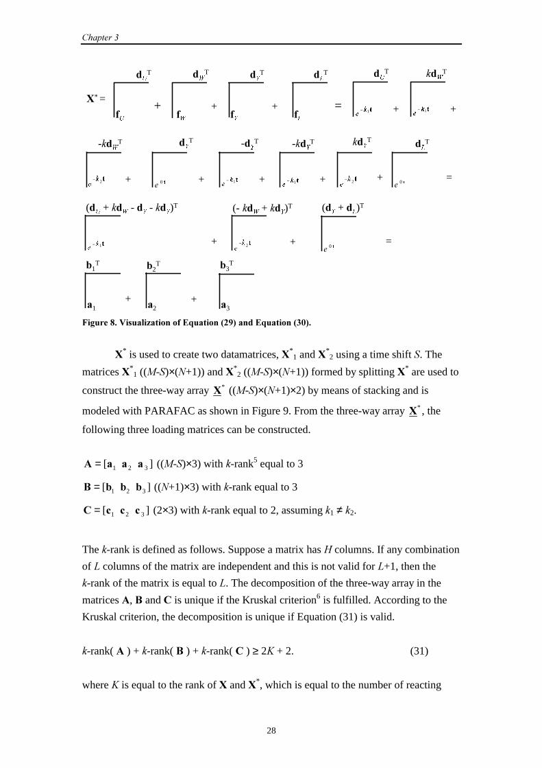
where W1N�− is a shorthand notation for [ QWNWN �� 111 ... −− ], W2N�− is a shorthand notation for

[ QWNWN �� 212 ... −− ], � W

11= −� N , W� 2

2N�−= , � W

30= � , TT

1 )(<<:8

�� & −−+= ,

TT2 )(

<:�� & +−= and TT

3 )(/<��& += . Equation (29) and the mathematical

manipulation in Equation (30) are visualized in Figure 8. The concentration profiles,

8, : and <, are rearranged into the exponential functions �1, �2 and �3. The response

matrix #* consists of a sum of exponential functions.

��

28

+ + 8

�8

T �:

T �<

T

:

<

+

�/

T

/

#* == + +

�8

T ��:

T

-��:

T

+

-�<

T

H

N− 1WH

N− 1W

W2NH

−H

N− 1W+

�<

T

� 0 W+

�/

T

+

-��<

T

H

N− 1W

��<

T

+ =

HN− 1W

(�8 + ��

: - �

< - ��

<)T (- ��

: + ��

<)T

+

(�< + �

/)T

+ =

&1T &2

T

+

&3T

+�1 �2 �3

� 0 W

� 0 W

W2NH

−

W2NH

−

!��.��+��,�� '/��0�1-��'/��02-�

#* is used to create two datamatrices, #*1 and #*

2 using a time shift �. The

matrices #*1 ((�-�)×(�+1)) and #*

2 ((�-�)×(�+1)) formed by splitting #* are used to

construct the three-way array #* ((�-�)×(�+1)×2) by means of stacking and is

modeled with PARAFAC as shown in Figure 9. From the three-way array #* , the

following three loading matrices can be constructed.

� � �� = [ ]1 2 3 ((�-�)×3) with �-rank5 equal to 3

3 & ��& ��&= [ ]1 2 3 ((�+1)×3) with �-rank equal to 3

� � �� = [ ]1 2 3 (2×3) with �-rank equal to 2, assuming �1 ≠ �2.

The �-rank is defined as follows. Suppose a matrix has $ columns. If any combination

of # columns of the matrix are independent and this is not valid for #+1, then the

�-rank of the matrix is equal to #. The decomposition of the three-way array in the

matrices �, 3 and � is unique if the Kruskal criterion6 is fulfilled. According to the

Kruskal criterion, the decomposition is unique if Equation (31) is valid.

�-rank( � ) + �-rank( 3 ) + �-rank( � ) ≥ 2% + 2. (31)

where % is equal to the rank of # and #*, which is equal to the number of reacting

��

29

= +

+

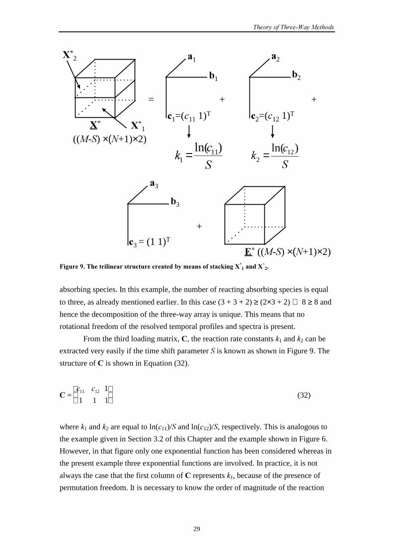
'4�((�-�) ×(�+1)×2)

#*

&1

&3

&2

+

#*1

#*2

�3 = (1 1)T

�1=(�11 1)T

�2�1

�3

((�-�) ×(�+1)×2)

�2=(�12 1)T

��

�)ln( 11

1 =�

��

)ln( 122 =

!��1� ��&��%�� )��#

��#

��

absorbing species. In this example, the number of reacting absorbing species is equal

to three, as already mentioned earlier. In this case (3 + 3 + 2) ≥ (2×3 + 2) ⇒ 8 ≥ 8 and

hence the decomposition of the three-way array is unique. This means that no

rotational freedom of the resolved temporal profiles and spectra is present.

From the third loading matrix, �, the reaction rate constants �1 and �2 can be

extracted very easily if the time shift parameter � is known as shown in Figure 9. The

structure of � is shown in Equation (32).

� =� �11 12 1

1 1 1

(32)

where �1 and �2 are equal to ln(�11)/� and ln(�12)/�, respectively. This is analogous to

the example given in Section 3.2 of this Chapter and the example shown in Figure 6.

However, in that figure only one exponential function has been considered whereas in

the present example three exponential functions are involved. In practice, it is not

always the case that the first column of � represents �1, because of the presence of

permutation freedom. It is necessary to know the order of magnitude of the reaction

��

30

rate constants in advance to judge which column represents �1, for example. So far,

the whole procedure is valid if #* is splitted into two datasets.

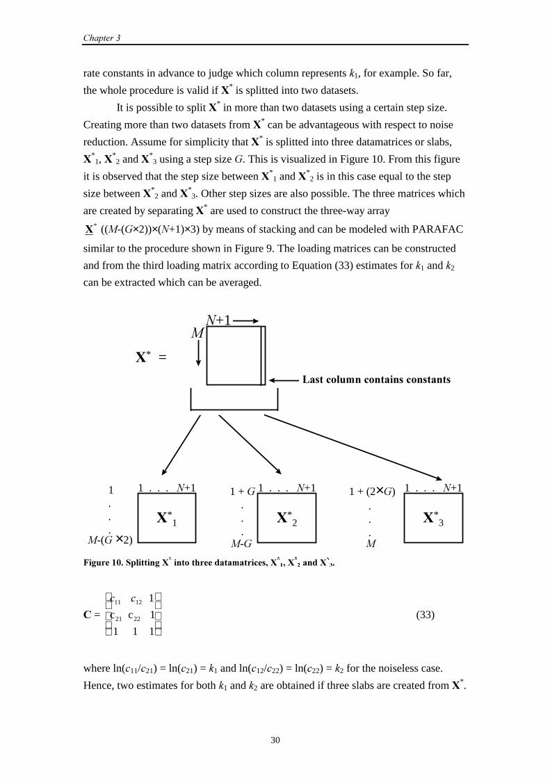
It is possible to split #* in more than two datasets using a certain step size.

Creating more than two datasets from #* can be advantageous with respect to noise

reduction. Assume for simplicity that #* is splitted into three datamatrices or slabs,

#*1, #

*2 and #*

3 using a step size &. This is visualized in Figure 10. From this figure

it is observed that the step size between #*1 and #*

2 is in this case equal to the step

size between #*2 and #*

3. Other step sizes are also possible. The three matrices which

are created by separating #* are used to construct the three-way array

#* ((�-(&×2))×(�+1)×3) by means of stacking and can be modeled with PARAFAC

similar to the procedure shown in Figure 9. The loading matrices can be constructed

and from the third loading matrix according to Equation (33) estimates for �1 and �2

can be extracted which can be averaged.

#*1

1...

1 . . . �+1

�-(&�×2)

#* =

�

#*2

1 . . . �+1

5��%��

�+1

#*3

1 + (2×&) . . .

1 . . . �+1

�

1 + & . . .�-&

!��2��# ��%��6�#

�6�#

��#

��

� =

� �11 12 1

c c 1

1 1 121 22

(33)

where ln(�11/�21) = ln(�21) = �1 and ln(�12/�22) = ln(�22) = �2 for the noiseless case.

Hence, two estimates for both �1 and �2 are obtained if three slabs are created from #*.

��

31

These estimates can be averaged. Likewise, three estimates of reaction rate constants

are obtained from four slabs, etc…

The trilinear structure discussed in this Section is the root of the non-iterative

and the iterative algorithms which are discussed in the next Sections. However, using

these algorithms it is necessary that the exponential functions involved have to be

written as a sum of exponential functions. This is a drawback, because that makes

three-way modelling as presented in this Chapter only suitable for (pseudo-) first order

kinetic problems. In case of, for example, second order kinetics two-way methods

described in the previous Chapter have to be used to obtain reaction rate constant

estimates.

�"�7��8�� %��

Consider again the two reaction steps from the reaction, described in Section 2.2 of

Chapter 2, under pseudo-first order conditions and matrix # with spectroscopic

measurements of the reaction. Two slabs are created from #* resulting in the

three-way array #* ((�-�)×(�+1)×2). From this structure the reaction rate constants

can be estimated according to the following steps.

1) Start with a generalized eigenvalue problem (GEP)7 which gives the two loading

matrices � and 3. The third loading matrix, �, is obtained by a least squares step. In

order to solve the GEP, the matrices #*1 and #*

2 need to be transferred into square

matrices. This can be done by using a common space8 onto which both matrices are

projected. In this paper, the common space was based on #*1 + #*

2.

2) Recognize the triad which is constant and permute the model such that the third

triad models the added constant. For the noiseless case or in case of adding a column

with constants (soft constraint), where the order of magnitude of the constants is large

compared to the order of magnitude of the signal in #, the third column of �, �3, is

constant and vector �3, the third column of �, is equal to (1 1)T. In case of adding a

column with constants, where the order of magnitude of the constants is comparable

to the order of magnitude of the signal, the third column of � is not equal to (1 1)T. If

the order of magnitude of the reaction rate constants is known in advance, the reaction

rate constants �1 and �2 can be estimated directly from the scaling factors listed in the

first two columns of the � matrix if the time shift is known.

Note, that the GEP not always gives satisfactory results, because it can

produce complex results. The third column of � and � are known beforehand.

��

32

However, this knowledge cannot be implemented at first sight. However, if a column

with constants is added to # as mentioned earlier, the third column of � and � are

forced to be constant. In case of data with a moderate signal to noise ratio, the third

column of the two matrices is often not constant. That problem is solved by adding a

column with constants to #, where the order of magnitude of the constant is large

compared to the signal present in #. Using this approach, the columns are forced to be

constant. Comparing the results of GEP with the third column of � and � gives a

check on the quality of the results obtained.

The procedure described is a modification of the generalized rank annihilation

method (GRAM). In this thesis, the modified GRAM procedure is just called GRAM.

Windig and Antalek used this new GRAM procedure for obtaining parameters from

NMR signals.9,10 They called the new procedure the direct exponential curve

resolution algorithm (DECRA). GRAM is a non-iterative algorithm and hence no

starting values are needed for the reaction rate constants. The time necessary to obtain

the reaction rate constants is known in advance. These properties make GRAM

suitable for cases where fast estimates of parameters are desired.

Consider that three slabs are created from #* resulting in the three-way array

#* ((�-(&×2))×(�+1)×3). It is not possible to estimate reaction rate constants using

GRAM. In this case, the trilinear decomposition (TLD) algorithm which is well

described in the literature by Booksh ��'(,11 has to be used. Here, a short description

is given.

1) The three-way array #* ((�-(&×3))×(�+1)×3) is decomposed into three loading

matrices �, 3 and �. The matrices � and 3 are both obtained by solving a GEP and �

is obtained by means of a three-way least squares fit (PARAFAC fit) from #* , � and

3. A common space of #*1 + #*

3 is used for solving the GEP.

2) Estimate the reaction rate constants from the scaling factors listed in �.

3) Average the estimates for �1 and �2. This yields a mean estimated �1 and �2.

Also in case of TLD the time needed to obtain the reaction rate constants is

known in advance and because of the non-iterative nature of the algorithm no starting

values are required for the kinetic parameters.

��

33

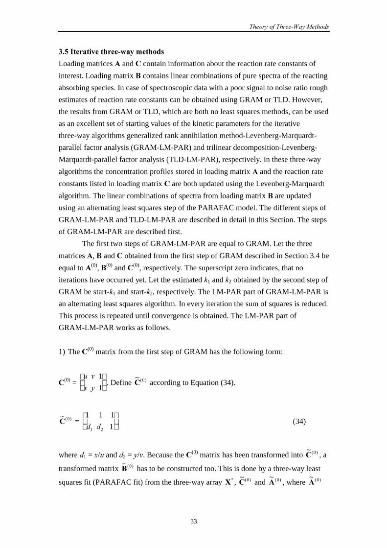
�$��8�� %��

Loading matrices � and � contain information about the reaction rate constants of

interest. Loading matrix 3 contains linear combinations of pure spectra of the reacting

absorbing species. In case of spectroscopic data with a poor signal to noise ratio rough

estimates of reaction rate constants can be obtained using GRAM or TLD. However,

the results from GRAM or TLD, which are both no least squares methods, can be used

as an excellent set of starting values of the kinetic parameters for the iterative

three-way algorithms generalized rank annihilation method-Levenberg-Marquardt-

parallel factor analysis (GRAM-LM-PAR) and trilinear decomposition-Levenberg-

Marquardt-parallel factor analysis (TLD-LM-PAR), respectively. In these three-way

algorithms the concentration profiles stored in loading matrix � and the reaction rate

constants listed in loading matrix � are both updated using the Levenberg-Marquardt

algorithm. The linear combinations of spectra from loading matrix 3 are updated

using an alternating least squares step of the PARAFAC model. The different steps of

GRAM-LM-PAR and TLD-LM-PAR are described in detail in this Section. The steps

of GRAM-LM-PAR are described first.

The first two steps of GRAM-LM-PAR are equal to GRAM. Let the three

matrices �, 3 and � obtained from the first step of GRAM described in Section 3.4 be

equal to �(0), 3(0) and �(0), respectively. The superscript zero indicates, that no

iterations have occurred yet. Let the estimated �1 and �2 obtained by the second step of

GRAM be start-�1 and start-�2, respectively. The LM-PAR part of GRAM-LM-PAR is

an alternating least squares algorithm. In every iteration the sum of squares is reduced.

This process is repeated until convergence is obtained. The LM-PAR part of

GRAM-LM-PAR works as follows.

1) The �(0) matrix from the first step of GRAM has the following form:

�(0) = )��*

��

1

1

. Define

~ ( )� 0 according to Equation (34).

~ ( )� 0 = 1 1 1

11 2� �

(34)

where �1 = �/) and �2 = �/*. Because the �(0) matrix has been transformed into ~ ( )� 0 , a

transformed matrix ~ ( )3 0 has to be constructed too. This is done by a three-way least

squares fit (PARAFAC fit) from the three-way array #* , ~ ( )� 0 and

~ ( )� 0 , where ~ ( )� 0

��

34

is a matrix with the reconstructed exponentially decaying functions using start-�1 and

start-�2 for �1 and �2, respectively, according to Equation (35).

~[~~

, ] [~~

, ~~ , ]( ) ( ) ( ) ( ) ( ) ( )� � � � � �0 030

10

20

30= = (35)

where the matrix with a double tilde consist of the first two columns of the considered

matrix, W� 1)0(1

~~ N�−= and W� 2)0(2

~~ N�−= . The vector T)...( )(111 60WNWN �� −−− is reduced to the

shorthand notation � N− 1W and T)(1 )...(60

−=� . The first two columns of ~ ( )� 0 , )0(

~~� , are

a function of �1 and �2, respectively and, hence, these are a function of �1, �2 and �.

The third column of ~ ( )� 0 , �3

(0), is constant. This column is fixed during the

GRAM-LM-PAR algorithm.

2) Matricize #* into ~ *# ((�-�)×(2�+2)). In chemometrics matricizing is often

denoted as “unfolding”. However, in psychometrics this has another meaning.12

Subtract the contribution of the columns of constants from ~ *# resulting in

� *# ((�-�)×(2�+2)).

T)0(3

)0(3

)0(3

*)0*( )~

(~

&��## ⊗−=� (36)

where ⊗ denotes the Kronecker product12 and �3 is the third column of )0(~� equal to

T)11( �� .

3) Next, matrices are partitioned:

~ ( )3 0 = [~~

,~

]( ) ( )3 &03

0 (37)

~ ( )� 0 = [~~ ( )� 0 ,

1

1

] (38)

where the matrices with a double tilde consist of the first two columns of the

considered matrix.

4) Equation (39) is minimized for fixed )0(~~3 over �1 and �2 ensuring that for the

proper �1 and �2 this minimum will be attained.

��

35

(39)2

T)0()0()0()0(*

ˆ,ˆ)

~~~~(

~~min

21

3��# −�NN

�

where � denotes the column-wise Kronecker product also known as the Khatri-Rao

product.12

Update ~~ ( )� 0 and

~~ ( )� 0 simultaneously using the optimal values for �1 and �2 according

to the Levenberg-Marquardt algorithm.

5) Update ~ ( )3 0 (all three columns!) using a least-squares PARAFAC step.

6) Calculate the loss function according to Equation (40).

(40)))~~~~

(~~

( T)()()()(*)( LLLLL ��,� 3��# −= � �

where SSQ is the sum of squares. If Equation (41) holds the iterations are stopped.

� ��

L L

L

( ) ( )

( )

−−−

<1

610 (41)

The TLD-LM-PAR algorithm is exactly the same algorithm as

GRAM-LM-PAR except that in TLD-LM-PAR the TLD results are used as an initial

set of starting values for �1 and �2 instead of the GRAM results for the reaction rate

constants. Only the first two steps of the TLD-LM-PAR algorithm differ from those of

the GRAM-LM-PAR algorithm. For TLD-LM-PAR the first two steps are given

below.

1) Applying TLD gives loading matrices �(0), 3(0), �(0) and multiple reaction rate

constant estimates. The reaction rate constant estimates are averaged resulting in ��1

and 2� .

2) Define ~ ( )� 0 ,

~ ( )3 0 and ~ ( )� 0 . The first column of �(0) represents W1N�− and the second

column of �(0) represents W2N�− . Hence, �1 and �2 can be replaced by ��1 and 2� ,

respectively, resulting in ~ ( )� 0 which is a reconstruction of the concentration profiles

using the averaged reaction rate constant estimates. ~ ( )� 0 is a reconstruction of �(0)

��

36

where the last row and last column are set to a row vector and a column vector of

ones, respectively, and ��1 and 2� are used for the reconstruction of �(0). Matrix ~ ( )3 0

is constructed by means of a three-way least squares fit (PARAFAC fit) from #* ,~ ( )� 0 and

~ ( )� 0 .

The next steps are equal to the GRAM-LM-PAR algorithm.

�(��8��

If reaction rate constants are estimated with GRAM, TLD, GRAM-LM-PAR or

TLD-LM-PAR, the relative fit error can be estimated. This is done as follows.

Matricize the three-way matrix #* resulting in #~

. Estimate #~

, #~

, according to

Equation (42).

(42)T* )~~

(~~

3��# = �

Delete the two columns with constants from #~

and #~

to construct

#� ((�-�)×2�) and #� ((�-�)×2�), respectively. The relative fit error (RFE) can be

estimated according to Equation (43).

∑∑

∑∑

= =

= =

−=

,

L

-

M

LM

,

L

-

M

LM

1 1

2

1 1

2

)(

)ˆ(

RFE#

##

�

��

(43)

where - = (�-�), . = 2�, / = 1, 2, …, - and 0 = 1, 2, …, .. From Equation (43) it can be

seen that it is necessary to delete the columns with constants from the two-way arrays,

because otherwise the denominator will dominate.

�*��%��%��

The use of constraint R, constraint RP and constraint NNLS, as discussed in Section

2.7 of Chapter 2, is only possible for the iterative three-way methods

(GRAM-LM-PAR and TLD-LM-PAR). Using ��/��/ known pure spectra of reacting

absorbing species within three-way methods is more complicated compared to

��

37

two-way methods, because loading matrix 3 contains linear combinations of pure

spectra. The use of pure spectra of reacting absorbing species as constraints in

iterative three-way methods is beyond the scope of this thesis.

In case of non-iterative three-way methods (GRAM and TLD), the following

soft constraint is implemented. The third column of loading matrix � is forced to be

constant by means of adding a column with constants to matrix #, where the order of

magnitude of the constants is large compared to the order of magnitude of the signal

in #.

The following constraints have been used in this thesis in case of

GRAM-LM-PAR and TLD-LM-PAR. The third column of loading matrix � and

loading matrix � are fixed during the whole least squares part of the three-way

algorithms. In case of GRAM-LM-PAR and TLD-LM-PAR the structure of � given

in Equation (32) and Equation (33), respectively, is implemented.

�.��9� ��1. Antalek B, Windig W. ‘Generalized rank annihilation method applied to a single multicomponent

pulsed gradient spin echo NMR data set’. .(�1�(��(��(, 1996; ��.: 10331-10332.

2. Windig W, Antalek B. ‘Direct exponential curve resolution algorithm (DECRA): A novel

application of the generalized rank annihilation method for a single spectral mixture data set with

exponentially decaying contribution profiles’. ��/��- �''(�#��(��(, 1997; *: 241-254.

3. Harshman RA, Lundy ME. ‘PARAFAC: Parallel factor analysis’. ��)�/� �'��/�/��2�3��

1 �'��/�, 1994, �.: 39-72.

4. Smilde AK. ‘Three-way analyses problems and prospects’. ��/��- �''(�#��(��(, 1992;

�$: 143-157.

5. Kruskal JB. in �)'/4��3��1 �'��/�, ed. by Coppi R, Bolasco S. Elsevier: Amsterdam, 1989;

7-18.

6. Kruskal JB, Harshman RA, Lundy ME. in �)'/4��3��1 �'��/�, ed. by Coppi R, Bolasco S.

Elsevier: Amsterdam, 1989; 115-122.

7. Sanchez E, Kowalski BR. ‘Generalized rank annihilation factor analysis’. 1 �'(��(, 1986; $.:

496-499.

8. Wilson B, Sanchez E, Kowalski BR. ‘An improved algorithm for the generalized rank annihilation

method’. .(��/��, 1989; : 493-498.

9. Windig W, Hornak JP, Antalek B. ‘Multivariate image analysis of magnetic resonance images with

the direct exponential curve resolution algorithm (DECRA). Part 1: Algorithm and model study’.

.(��5 (�� (, 1998; ��: 298-306.

10. Antalek B, Hornak JP, Windig W. ‘Multivariate image analysis of magnetic resonance images with

the direct exponential curve resolution algorithm (DECRA). Part 2: Application to human brain

images’. .(��5 (�� (, 1998; ��: 307-315.

11. Booksh KS, Lin Z, Wang Z, Kowalski BR. ‘Extension of trilinear decomposition method with an

application to the flow probe sensor’. 1 �'(��(, 1994; ((: 2561-2569.

12. Kiers HAL. ‘Towards a standardized notation and terminology in multiway analysis’.

.(��/��, 2000; in press.

��

38

39

��

��

��

��

If reaction rate constants are estimated from spectroscopic data of repeated batch runs,

these estimates have a certain accuracy. The accuracy of reaction rate constant

estimates is influenced by model errors, experimental errors and instrumental noise

which are always present. Examples of experimental errors are: initial concentration

errors of reactants at the start of the reaction and temperature fluctuations during the

reaction. Instrumental noise is caused by variations of the instrument. If, for example,

a suitable kinetic model for the data is used and the Beer-Lambert law is valid, model

errors can be kept very small compared to experimental errors and instrumental noise.

Assume a batch process with reaction rate constant �1. Suppose that model

errors are negligible compared to the experimental errors and instrumental noise

present. For each individual batch process run the reaction rate constant, �1, can be

estimated. A standard deviation can be obtained, from the �1 estimates of � repeated

individual batch process runs, which represents the upper error bound.

A lower level of standard deviation, the lower error bound, represents the

influence of mainly instrumental noise on the �1 estimates. It can be estimated using a

jackknife based resampling method described in Section 4.3.1,2

��

The accuracy of a parameter can be divided into the precision and the bias of the

parameter according to equation (44).

222 ))ˆ(())ˆ(ˆ()ˆ(WUXHWUXH�� −+−=− (44)

��

where � indicates the expectation operator. The accuracy, bias and precision of a

parameter can be estimated by applying Equation (45), (46) and (47), respectively.

��

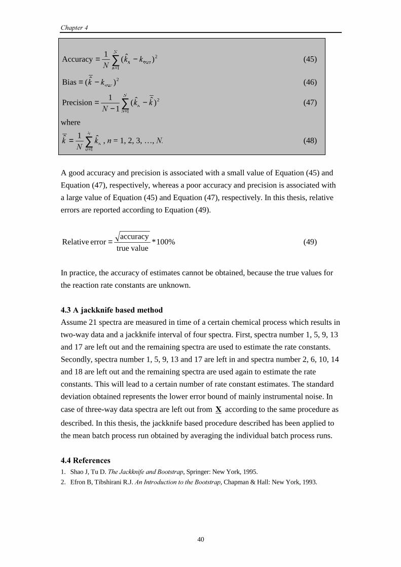
40

∑=

−=1

Q

WUXHQ��

1

2)ˆ(1

Accuracy (45)

2)ˆ(BiasWUXH�� −= (46)

∑=

−−

=1

Q

Q��

1

2)ˆˆ(1

1Precision (47)

where

∑=

=1

Q

Q�

�

1

ˆ1ˆ , � = 1, 2, 3, …, � (48)

A good accuracy and precision is associated with a small value of Equation (45) and

Equation (47), respectively, whereas a poor accuracy and precision is associated with

a large value of Equation (45) and Equation (47), respectively. In this thesis, relative

errors are reported according to Equation (49).

%100* valuetrue

accuracy error Relative = (49)

In practice, the accuracy of estimates cannot be obtained, because the true values for

the reaction rate constants are unknown.

�� !!� ��"��

Assume 21 spectra are measured in time of a certain chemical process which results in

two-way data and a jackknife interval of four spectra. First, spectra number 1, 5, 9, 13

and 17 are left out and the remaining spectra are used to estimate the rate constants.

Secondly, spectra number 1, 5, 9, 13 and 17 are left in and spectra number 2, 6, 10, 14

and 18 are left out and the remaining spectra are used again to estimate the rate

constants. This will lead to a certain number of rate constant estimates. The standard

deviation obtained represents the lower error bound of mainly instrumental noise. In

case of three-way data spectra are left out from # according to the same procedure as

described. In this thesis, the jackknife based procedure described has been applied to

the mean batch process run obtained by averaging the individual batch process runs.

��1. Shao J, Tu D. ��, Springer: New York, 1995.

2. Efron B, Tibshirani R.J. ��, Chapman & Hall: New York, 1993.

41

��

��

��

��

In this Chapter, four different experimental datasets used in this thesis are described.

A short summary of the datasets can be found in the Appendix. Dataset 1 contains

short-wavelength near-infrared (SW-NIR)1,2 measurements of a two-step epoxidation

performed under pseudo-first order conditions. Dataset 2 contains ultraviolet-visible

(UV-Vis)1,2 measurements of a two-step biochemical reaction also performed under

pseudo-first order conditions at a certain pH. At a different pH the same reaction has

been monitored using UV-Vis spectroscopy performed under pseudo-first order

conditions and second order conditions, resulting in dataset 3 and dataset 4,

respectively.

For dataset 2, 3 and 4, pure spectra of some of the reacting absorbing species

involved in the reaction have been measured. This is described in this Chapter

together with the experimental set-up, dataprocessing and the repeatability of

experiments.

��

��

The two-step consecutive epoxidation of 2,5-di- � -butyl-1,4-benzoquinone using

� -butyl hydroperoxide and Triton B catalyst3,4 was monitored in time using

SW-NIR spectroscopy. The reaction consists of the following two steps:i

� + � → DN � + �

� + � → EN � + �

i In this thesis, reaction rate constants with Arabic subscript are second order reaction rate constants and

reaction rate constants with numerical subscript are (pseudo-) first order reaction rate constants.

��

42

with second order reaction rate constants �a and �b both in M-1min-1. Species �, �, �,

� and � are specified in Table 1.

�!�� "��"�� #�$�%��

Species

� 2,5-di- � -butyl-1,4-benzoquinone

� � -butyl hydroperoxide

� 2,5-di- � -butyl mono-epoxide-1,4-benzoquinone

� cis and trans 2,5-di- � -butyl di-epoxide-1,4-benzoquinone

� � -butyl alcohol

No distinction was made between the cis and trans product (species �) of the second

step of the reaction, because the spectral differences are negligible in SW-NIR.4

The first and second reaction step are both second order reactions. However, if

species � is present in large excess, the first and second reaction step become both

pseudo-first order reactions with pseudo-first order reaction rate constants �1 (min-1)

and �2 (min-1), respectively. Hence, Equation (6)-(8), defined in Section 2.2 of

Chapter 2, can be used in order to describe the concentration profiles of the reactant

(species �), intermediate (species �) and main-product (species �) of the reaction,

respectively.

��

A cuvette was filled with 0.264 g (1.2 mmol) of 2,5-di- � -butyl-1,4-benzoquinone,

as synthesized by the procedure described by Hairfield � ��.3 A melting point of

152-153°C was obtained for 2,5-di- � -butyl-1,4-benzoquinone. The reported melting

point is 152.5°C.5 Next, 2,5-di- � -butyl-1,4-benzoquinone was dissolved in 15 ml

dioxane (Acros 99+%) and 1.55 ml (12 mmol) of a � -butylhydroperoxide 70%

(Acros) solution in water and 13.21 ml ethanol (BDH Laboratory Supplies, pro

analysis) were both added. After the target reaction temperature had been reached,

data collection was started immediately after addition of 0.24 ml ice-cold Triton B

catalyst (Acros, 40 wt. % in methanol) in 0.50 ml ethanol and 0.60 ml dioxane. The

excess of � -butylhydroperoxide in moles was ten times

2,5-di- � -butyl-1,4-benzoquinone. At this excess, pseudo-first order kinetics may be

assumed.

��

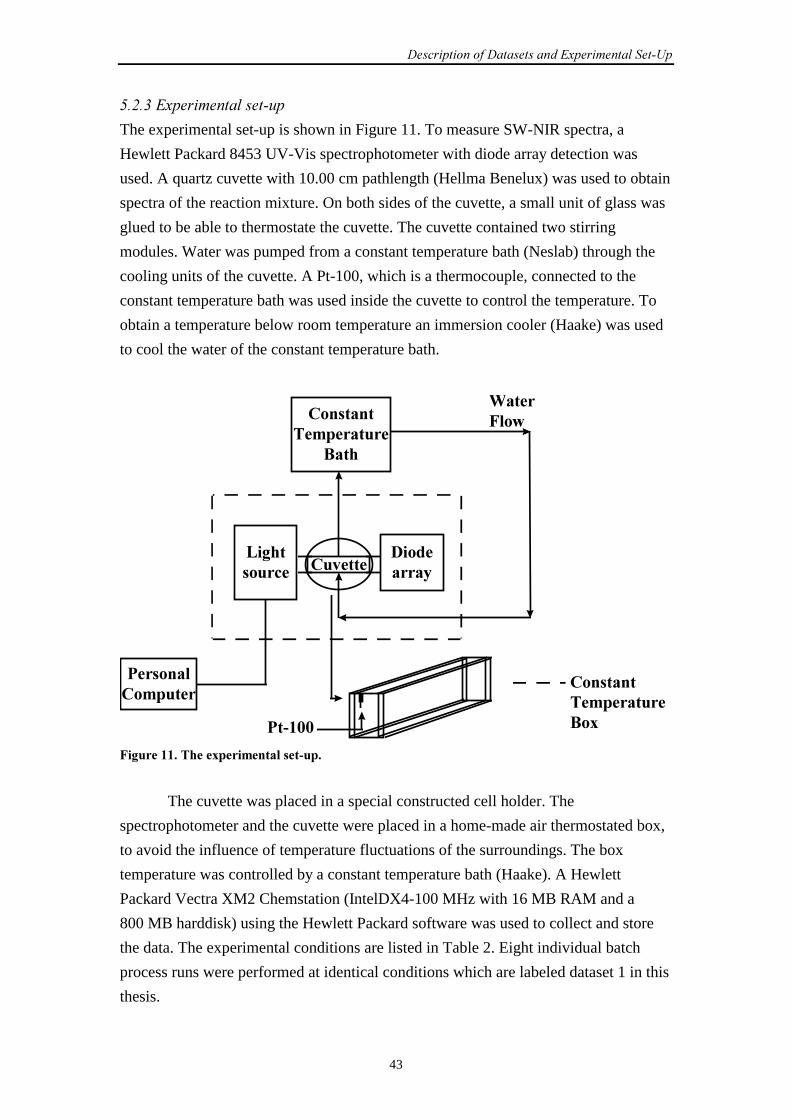
43

��!�� "�

The experimental set-up is shown in Figure 11. To measure SW-NIR spectra, a

Hewlett Packard 8453 UV-Vis spectrophotometer with diode array detection was

used. A quartz cuvette with 10.00 cm pathlength (Hellma Benelux) was used to obtain

spectra of the reaction mixture. On both sides of the cuvette, a small unit of glass was

glued to be able to thermostate the cuvette. The cuvette contained two stirring

modules. Water was pumped from a constant temperature bath (Neslab) through the

cooling units of the cuvette. A Pt-100, which is a thermocouple, connected to the

constant temperature bath was used inside the cuvette to control the temperature. To

obtain a temperature below room temperature an immersion cooler (Haake) was used

to cool the water of the constant temperature bath.

& '��

��(��"��

��

)��

*��

*��++

�� )��

#��,��

, '��

The cuvette was placed in a special constructed cell holder. The

spectrophotometer and the cuvette were placed in a home-made air thermostated box,

to avoid the influence of temperature fluctuations of the surroundings. The box

temperature was controlled by a constant temperature bath (Haake). A Hewlett

Packard Vectra XM2 Chemstation (IntelDX4-100 MHz with 16 MB RAM and a

800 MB harddisk) using the Hewlett Packard software was used to collect and store

the data. The experimental conditions are listed in Table 2. Eight individual batch

process runs were performed at identical conditions which are labeled dataset 1 in this

thesis.

��

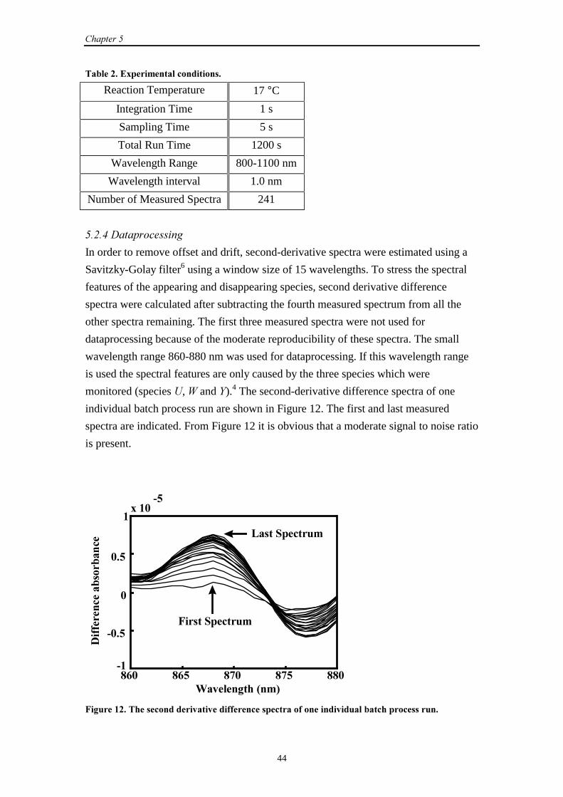
44

�!��

Reaction Temperature 17 °C

Integration Time 1 s

Sampling Time 5 s

Total Run Time 1200 s

Wavelength Range 800-1100 nm

Wavelength interval 1.0 nm

Number of Measured Spectra 241

��#�� $

In order to remove offset and drift, second-derivative spectra were estimated using a

Savitzky-Golay filter6 using a window size of 15 wavelengths. To stress the spectral

features of the appearing and disappearing species, second derivative difference

spectra were calculated after subtracting the fourth measured spectrum from all the

other spectra remaining. The first three measured spectra were not used for

dataprocessing because of the moderate reproducibility of these spectra. The small

wavelength range 860-880 nm was used for dataprocessing. If this wavelength range

is used the spectral features are only caused by the three species which were

monitored (species �, � and �).4 The second-derivative difference spectra of one

individual batch process run are shown in Figure 12. The first and last measured

spectra are indicated. From Figure 12 it is obvious that a moderate signal to noise ratio

is present.

-.+ -. -/+ -/ --+��

�+�

+

+�

��+

�

#�"��'��0��1

��!��!��

, ��

&��

, '�� "�� "�� " ��!��

��

45

In case of using the WCR algorithm, described in Section 2.6 of Chapter 2, the

datamatrix with measured spectra of the reacting system was truncated into three

singular values. For the two-way methods starting values of 0.30 min-1 and 0.05 min-1

were used for �1 and �2, respectively, based on the estimates of these reaction rate

constants obtained by others.3,4

Data processing was performed in the Matlab environment (Version 5.2, The

Mathworks Inc.) on a Pentium 133 MHz Computer with 64 MB RAM and a 1.2 GB

harddisk.

��%�� &�� '��

The repeatability, (batch, for ) batch process runs was calculated using Equation (50).7

%100*

1

1

2

batch 2

22∑=

−=

,

L

L)( (50)

where 2L is the spectral matrix for experiment � and 2 is the averaged spectral matrix

obtained from the ) individual experiments.

The repeatability was equal to 23.28% for dataset 1. This poor repeatability is

mainly a consequence of the small differences in absorbances of the species and the

error propagation due to taking the second derivative.

�3��! ��

��!��

The two-step consecutive reaction of 3-chlorophenylhydrazonopropane dinitrile with

2-mercaptoethanol8,9 was monitored using UV-Vis spectroscopy. The reaction

consists of the following two steps:

� + � → DN �

� → 2N � + �

with second order reaction rate constant �a (M-1min-1) and first order reaction rate

constant �2 (min-1). Species �, �, �, � and � are specified in Table 3.

If species � is present in large excess the first step of the reaction becomes

pseudo-first order with pseudo-first order reaction rate constant �1 (min-1). Hence,

Equation (6)-(8), from Section 2.2 of Chapter 2, can be used in order to describe the

��

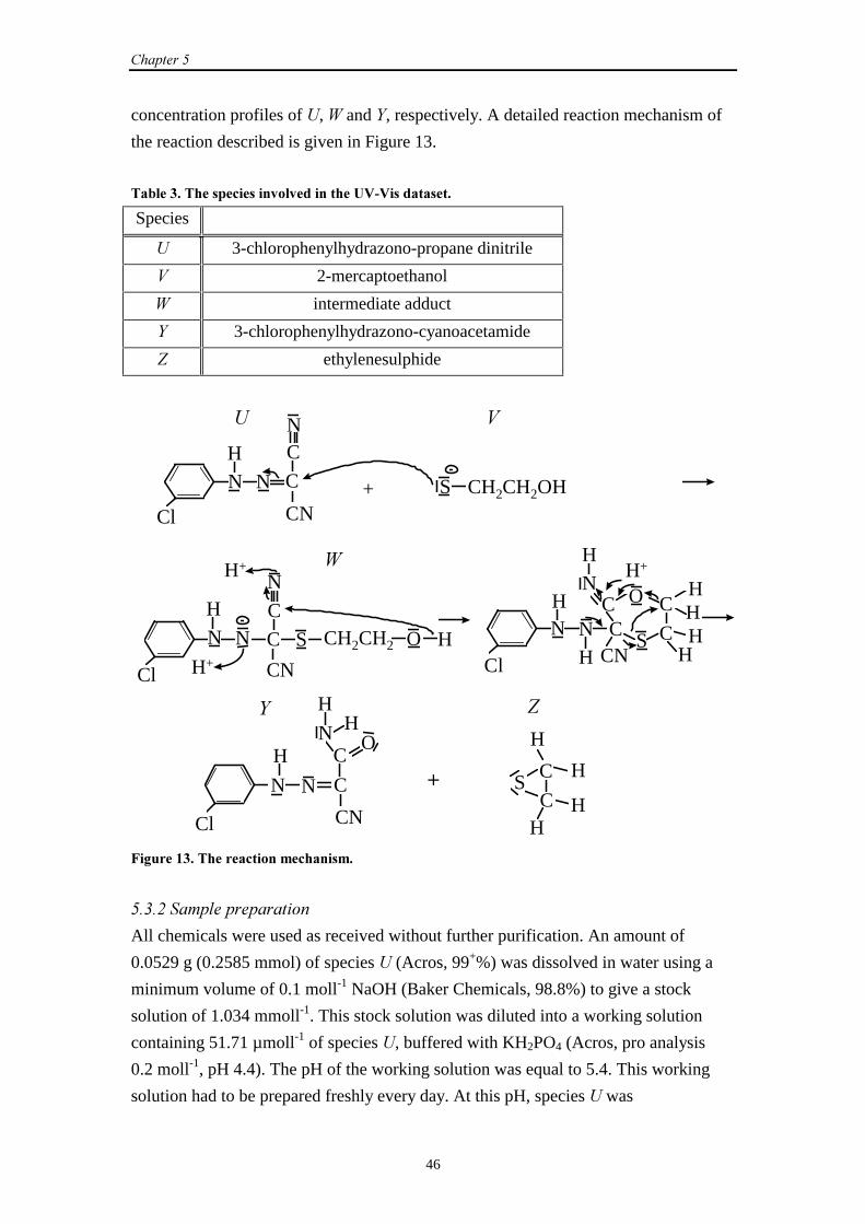
46

concentration profiles of �, � and �, respectively. A detailed reaction mechanism of

the reaction described is given in Figure 13.

�!��3�� "��"�� 4�4 ��

Species

� 3-chlorophenylhydrazono-propane dinitrile

� 2-mercaptoethanol

� intermediate adduct

� 3-chlorophenylhydrazono-cyanoacetamide

� ethylenesulphide

NH

N

C

CN

C

Cl+ CH2CH2OHS

N��

N

H

NC

CN

C

Cl

S CH2CH2

N

HO

H+

NH

NC

CNC

ClS C

H+ H

NO C

HHH

H

HH+�

N

H

N

C

CN

C

N O

Cl

HH

�

C

C

H

H

HH

S

�

5

, '��3��

��!��

All chemicals were used as received without further purification. An amount of

0.0529 g (0.2585 mmol) of species � (Acros, 99+%) was dissolved in water using a

minimum volume of 0.1 moll-1 NaOH (Baker Chemicals, 98.8%) to give a stock

solution of 1.034 mmoll-1. This stock solution was diluted into a working solution

containing 51.71 µmoll-1 of species �, buffered with KH2PO4 (Acros, pro analysis

0.2 moll-1, pH 4.4). The pH of the working solution was equal to 5.4. This working

solution had to be prepared freshly every day. At this pH, species � was

��

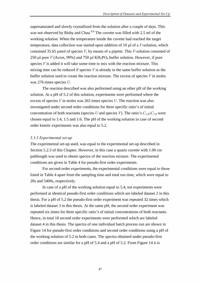
47

supersaturated and slowly crystallized from the solution after a couple of days. This

was not observed by Bisby and Chau.8,9 The cuvette was filled with 2.5 ml of the

working solution. When the temperature inside the cuvette had reached the target

temperature, data collection was started upon addition of 10 µl of a �-solution, which

contained 35.65 µmol of species �, by means of a pipette. This �-solution consisted of

250 µl pure � (Acros, 99%) and 750 µl KH2PO4 buffer solution. However, if pure

species � is added it will take some time to mix with the reaction mixture. This

mixing time can be reduced if species � is already in the same buffer solution as the

buffer solution used to create the reaction mixture. The excess of species � in moles

was 276 times species �.

The reaction described was also performed using an other pH of the working

solution. At a pH of 5.2 of this solution, experiments were performed where the

excess of species � in moles was 265 times species �. The reaction was also

investigated under second order conditions for three specific ratio’s of initial

concentration of both reactants (species � and species �). The ratio’s �8,0:�9,0 were

chosen equal to 1:4, 1:5 and 1:6. The pH of the working solution in case of second

order kinetic experiments was also equal to 5.2.

��!�!�� "�

The experimental set-up used, was equal to the experimental set-up described in

Section 5.2.3 of this Chapter. However, in this case a quartz cuvette with 1.00 cm

pathlength was used to obtain spectra of the reaction mixture. The experimental

conditions are given in Table 4 for pseudo-first order experiments.

For second-order experiments, the experimental conditions were equal to those

listed in Table 4 apart from the sampling time and total run time, which were equal to

20s and 5400s, respectively.

In case of a pH of the working solution equal to 5.4, ten experiments were

performed at identical pseudo-first order conditions which are labeled dataset 2 in this

thesis. For a pH of 5.2 the pseudo-first order experiment was repeated 32 times which

is labeled dataset 3 in this thesis. At the same pH, the second order experiment was

repeated six times for three specific ratio’s of initial concentrations of both reactants.

Hence, in total 18 second order experiments were performed which are labeled

dataset 4 in this thesis. The spectra of one individual batch process run are shown in

Figure 14 for pseudo-first order conditions and second order conditions using a pH of

the working solution of 5.2 in both cases. The spectra obtained under pseudo-first

order conditions are similar for a pH of 5.4 and a pH of 5.2. From Figure 14 it is

��

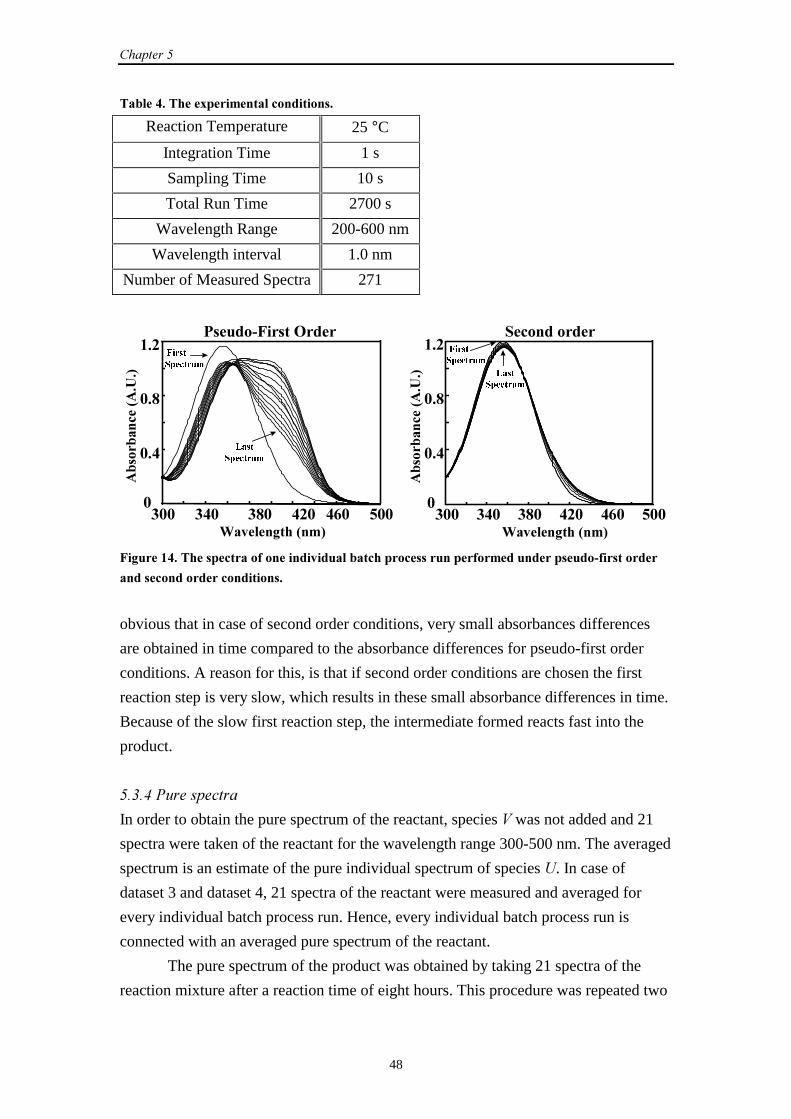
48

�!��6��

Reaction Temperature 25 °C

Integration Time 1 s

Sampling Time 10 s

Total Run Time 2700 s

Wavelength Range 200-600 nm

Wavelength interval 1.0 nm

Number of Measured Spectra 271

3++ 36+ 3-+ 6�+ 6.+ +++

+�6

+�-

��

#�"��'��0��1

�!��!��0��1

)LUVW

��6SHFWUXP

/DVW

6SHFWUXP

*��, ��7��

3++ 36+ 3-+ 6�+ 6.+ +++

+�6

+�-

��

#�"��'��0��1

)LUVW

��6SHFWUXP

/DVW

6SHFWUXP

��

�!��!��0��1

, '��6�� " ��!��

��

obvious that in case of second order conditions, very small absorbances differences

are obtained in time compared to the absorbance differences for pseudo-first order

conditions. A reason for this, is that if second order conditions are chosen the first

reaction step is very slow, which results in these small absorbance differences in time.

Because of the slow first reaction step, the intermediate formed reacts fast into the

product.

��!�#�*"��

In order to obtain the pure spectrum of the reactant, species � was not added and 21

spectra were taken of the reactant for the wavelength range 300-500 nm. The averaged

spectrum is an estimate of the pure individual spectrum of species �. In case of

dataset 3 and dataset 4, 21 spectra of the reactant were measured and averaged for

every individual batch process run. Hence, every individual batch process run is

connected with an averaged pure spectrum of the reactant.

The pure spectrum of the product was obtained by taking 21 spectra of the

reaction mixture after a reaction time of eight hours. This procedure was repeated two

��

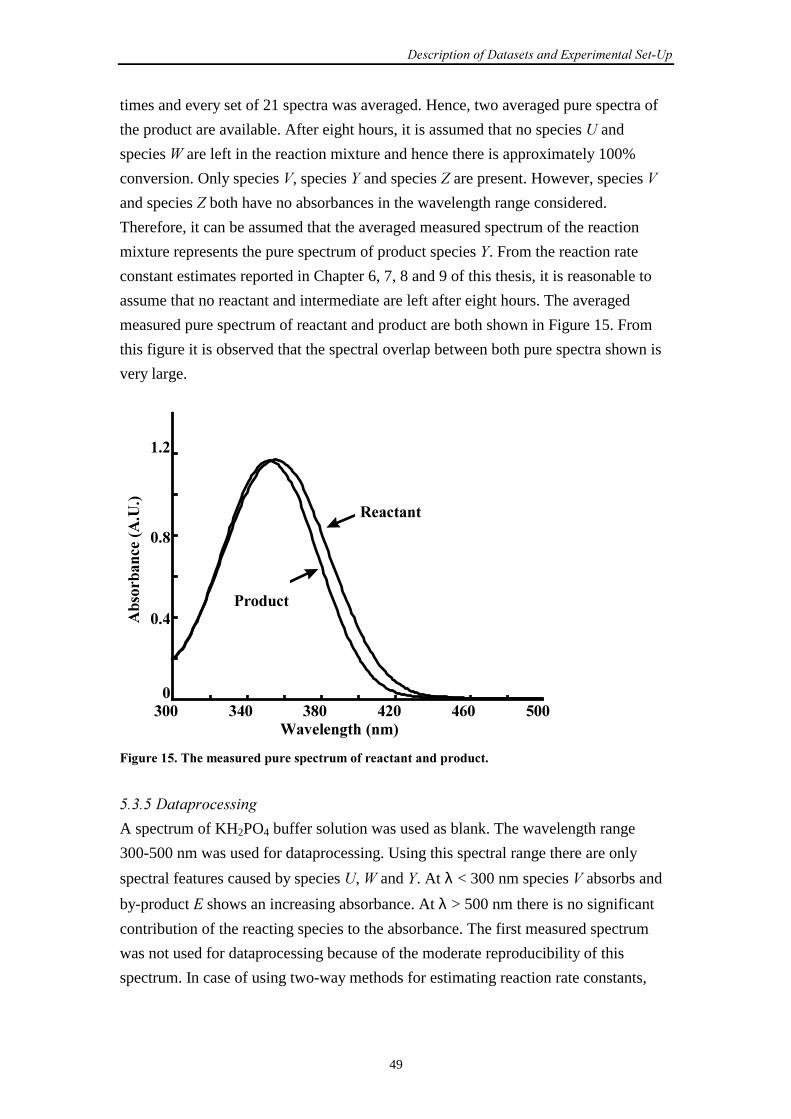
49

times and every set of 21 spectra was averaged. Hence, two averaged pure spectra of

the product are available. After eight hours, it is assumed that no species � and

species � are left in the reaction mixture and hence there is approximately 100%

conversion. Only species �, species � and species � are present. However, species �

and species � both have no absorbances in the wavelength range considered.

Therefore, it can be assumed that the averaged measured spectrum of the reaction

mixture represents the pure spectrum of product species �. From the reaction rate

constant estimates reported in Chapter 6, 7, 8 and 9 of this thesis, it is reasonable to

assume that no reactant and intermediate are left after eight hours. The averaged

measured pure spectrum of reactant and product are both shown in Figure 15. From

this figure it is observed that the spectral overlap between both pure spectra shown is

very large.

3++ 36+ 3-+ 6�+ 6.+ +++

+�6

+�-

��

#�"��'��0��1

�!��!��0��1

*��

%��

, '��

��!�� $

A spectrum of KH2PO4 buffer solution was used as blank. The wavelength range

300-500 nm was used for dataprocessing. Using this spectral range there are only

spectral features caused by species �, � and �. At λ < 300 nm species � absorbs and

by-product � shows an increasing absorbance. At λ > 500 nm there is no significant

contribution of the reacting species to the absorbance. The first measured spectrum

was not used for dataprocessing because of the moderate reproducibility of this

spectrum. In case of using two-way methods for estimating reaction rate constants,

��

50

starting values of 0.30 min-1 and 0.05 min-1 were used for �1 and �2, respectively,

based on the estimates obtained by others.8,9

Data processing was performed in the Matlab environment (Version 5.2, The

Mathworks Inc.) on a Pentium 133 MHz Computer with 64 MB RAM and a 1.2 GB

harddisk.

��!�+�%�� &�� '��

The repeatability was calculated for the UV-Vis datasets using Equation (50) from

Section 5.2.5 of this Chapter. The repeatability was equal to 0.54% and 1.60% for

dataset 2 and dataset 3, respectively. For dataset 4, three repeatability numbers were

calculated, because there were three different ratio’s of initial concentrations of the

reactants involved. For a ratio of 1:4, 1:5 en 1:6 the repeatability was equal to 1.28%,

2.15% and 1.15%, respectively. Hence, it can be concluded that dataset 3 and

dataset 4 have a similar repeatability. The repeatability of dataset 2 is excellent for

spectroscopic measurements.

�6�%��1. Workman JJ Jr. ‘Interpretive spectroscopy for near infrared’. ,�� (�-�, 1996; 3�:

251-320.

2. Burns DA, Ciurczak EW. .��&��/�� )��,��'��, Dekker: New York, 1992.

3. Hairfield EM, Moomaw EW, Tamburri RA, Vigil RA.�‘The epoxidation of

2,5-di-tert-butyl-1,4-benzoquinone’. 0��"� ��, 1985; .�: 175-177.


with shortwave near-infrared spectroscopy’, in /��)�� (�� '1�2��$��$� ��3��

&� 4�� ,��'��/)(�,�� , ed. by Hildrum KI, Isaksson T, Naes T, Tandberg A.


5. Weast RC. .��&�� '��*�'��, 1st Student Edition, Press CRC: Florida, 1988.

6. Savitzky A, Golay MJE. ‘Smoothing and differentiation of data by simplified least squares

procedures’. ,��, 1964; 3.: 1627-1639.

7. Smilde AK, Tauler R, Henshaw JM, Burgess LW, Kowalski BR. ‘Multicomponent Determination

of Chlorinated Hydrocarbons Using a Reaction-Based Chemical Sensor. 3. Medium-Rank Second-

Order Calibration with Restricted Tucker Models’. ,��, 1994; ..: 3345-3351.

8. Bisby RH, Thomas EW. ‘Kinetic analysis by the method of nonlinear least squares’. 0��

��"� ��, 1986; .3: 990-992.

9. Chau F-T, Mok K-W. ‘Multiwavelength analysis for a first-order consecutive reaction’. ��" ��

��, 1992; �.: 239-242.

51

��

��

��

In this Chapter,i the results of the two-way methods traditional curve fitting (TCF)

combined with fixed size window evolving factor analysis (FSWEFA), classical curve

resolution (CCR), weighted curve resolution (WCR) and curve resolution (CR),

applied to the four datasets described in Chapter 5, are presented. A short summary of

the four datasets is given in the Appendix. The theory of the two-way methods used

has already been described in Chapter 2 of this thesis. Note, that CR is the same

algorithm as WCR without weighting certain matrices during the optimization

procedure (see Section 2.6, Chapter 2). The starting values of the reaction rate

constants used for the two-way methods have been reported in Section 5.2.4 and

Section 5.3.5 of Chapter 5. If other sets of starting values were used, similar results

were obtained.

��

��

CR and WCR, which are described in Section 2.6 of Chapter 2, are applied to estimate

reaction rate constants from dataset 1. Dataset 1 contains SW-NIR measurements in

time of a two-step consecutive epoxidation reaction as described in Section 5.2 of

Chapter 5. Some simulations with synthetic spectra from a simple two-step process

i This Chapter is based on the following papers:

� Bijlsma S, Louwerse DJ, Smilde AK. ‘Rapid estimation of rate constants of batch processes using

on-line SW-NIR’. ��, 1998; !!: 2713-2723.

� Bijlsma S, Smilde AK. ‘Application of curve resolution based methods to kinetic data’. ��

� ��, 1999; "#: 231-240.

� Bijlsma S, Boelens HFM, Smilde AK. ‘Rapid determination of rate constants in second order kinetics’.

submitted.

� Bijlsma S, Boelens HFM, Hoefsloot HCJ, Smilde AK. ‘Estimating reaction rate constants: comparison

between traditional curve fitting and curve resolution’. submitted.

��

52

are used to show that the methods can be applied to estimate unknown reaction rate

constants in cases where the pure spectra of the reacting absorbing species involved

are extremely overlapped. For the reaction rate constant estimates obtained from

dataset 1, upper and lower error bounds are estimated in order to perform quality

assessment as described in Section 4.3 of Chapter 4. For the simulated data and

dataset 1, the performance of CR and WCR are compared.

��

For the simulations, the two-step consecutive reaction valid for dataset 1 was

considered. Concentration profiles (matrix $) were simulated for 21 time points for

species �, � and � corresponding to a �1 value of 0.30 min-1, a �2 value of 0.05 min-1

and an initial concentration of species � of 1 moll-1. The time range was chosen from

0 min to 20 min with increments of 1 min. Pure SW-NIR spectra (matrix %) were

simulated for the three individual reacting absorbing species for the wavelength range

850-1050 nm with increments of 1 nm using Gaussian peaks with a peak sigma of

15 nm. The maximum of the pure spectra of species �, � and � corresponded to

different wavelengths to control the amount of spectral overlap of the individual

spectra of these three species. The simulated spectra for datamatrix & were calculated

according to Equation (1) of Section 2.2, Chapter 2. Normally distributed white noise

was added to datamatrix &. The sigma of the white noise added was defined as a

certain percentage of the maximum absorbance of the simulated SW-NIR spectrum at

time 0.

The amount of spectral overlap presented in the pure SW-NIR spectra of the

different reacting absorbing species involved was varied by moving the individual

spectrum of species � and � along the wavelength axis. The pure spectra of the

individual reacting absorbing species with a small and a strong spectral overlap are

shown in Figure 16. A small spectral overlap corresponded to an absorbance

maximum of the pure spectra at 900 nm, 950 nm and 1000 nm for species �, � and �,

respectively (solid line). A strong overlap corresponded to a maximum of the pure

spectra at 930 nm, 950 nm and 970 nm for the species �, � and �, respectively

(dotted line). One hundred sets of SW-NIR spectra were simulated according to two

different noise levels (1% and 4%). For data reduction using the SVD, three singular

values were chosen, because three species were involved in the simulated SW-NIR

spectra. For every noise level 100 �1 and �2 values were estimated. The starting values

for �1 and �2 were always equal to 0.20 min-1 and 0.04 min-1, respectively.

�� !"��#�$��

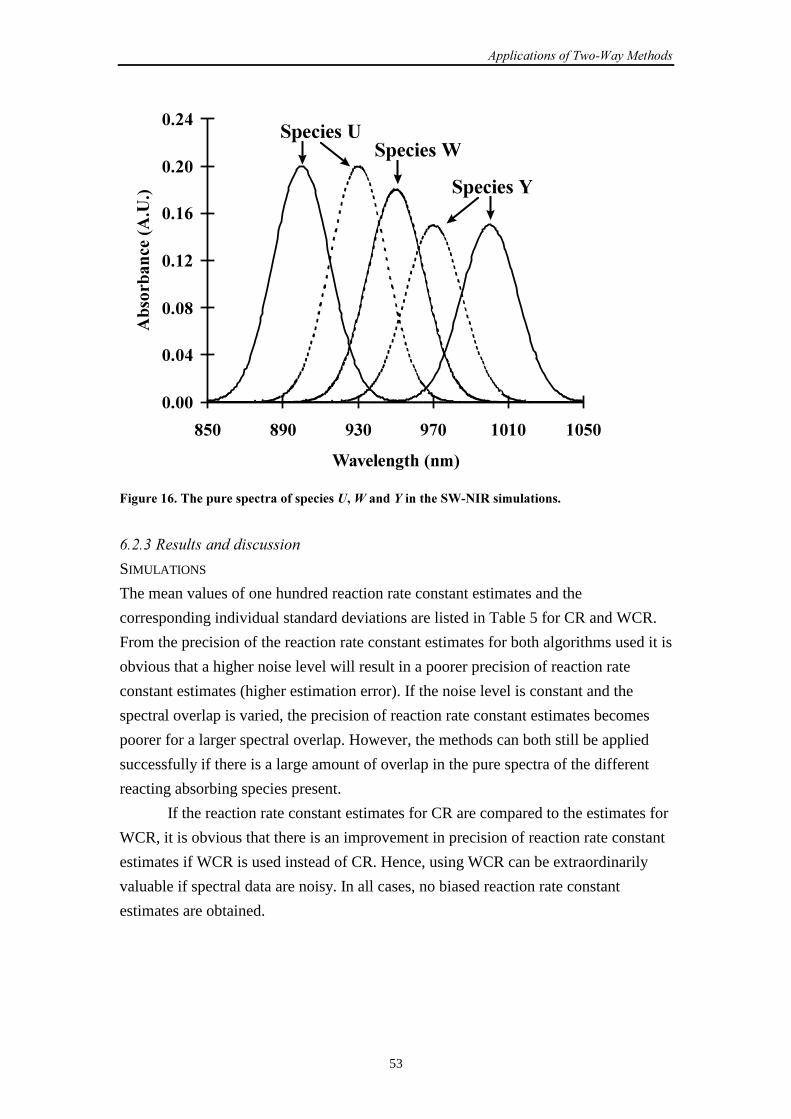
53

'�''

'�'!

'�'(

'��

'��

'��'

'��!

()' (#' #"' #*' �'�' �')'

��+��,��-�./

0��0�� -�1�/

�� 1��

�� 2

$�,�� 3�� .��

��%�&��

SIMULATIONS

The mean values of one hundred reaction rate constant estimates and the

corresponding individual standard deviations are listed in Table 5 for CR and WCR.

From the precision of the reaction rate constant estimates for both algorithms used it is

obvious that a higher noise level will result in a poorer precision of reaction rate

constant estimates (higher estimation error). If the noise level is constant and the

spectral overlap is varied, the precision of reaction rate constant estimates becomes

poorer for a larger spectral overlap. However, the methods can both still be applied

successfully if there is a large amount of overlap in the pure spectra of the different

reacting absorbing species present.

If the reaction rate constant estimates for CR are compared to the estimates for

WCR, it is obvious that there is an improvement in precision of reaction rate constant

estimates if WCR is used instead of CR. Hence, using WCR can be extraordinarily

valuable if spectral data are noisy. In all cases, no biased reaction rate constant

estimates are obtained.

��

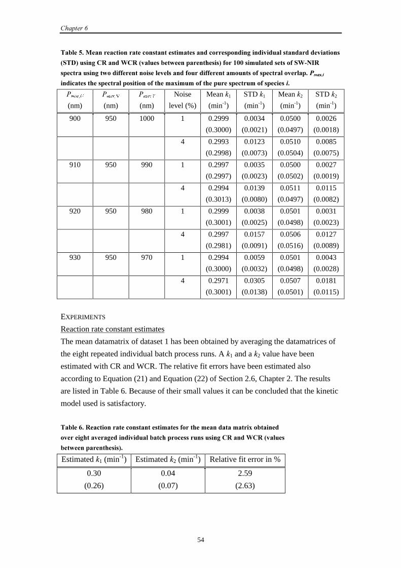
54

��0��)�� .�� ,��+��+��

-��%/��,�� -+��0��/��''��.��

�� ,��+��.�� +��PD[�L

�� .�4�.�.�� .��

'PD[�8

(nm)

'PD[�:

(nm)

'PD[�<

(nm)

Noise

level (%)

Mean �1

(min-1)

STD �1

(min-1)

Mean �2

(min-1)

STD �2

(min-1)

900 950 1000 1 0.2999

(0.3000)

0.0034

(0.0021)

0.0500

(0.0497)

0.0026

(0.0018)

4 0.2993

(0.2998)

0.0123

(0.0073)

0.0510

(0.0504)

0.0085

(0.0075)

910 950 990 1 0.2997

(0.2997)

0.0035

(0.0023)

0.0500

(0.0502)

0.0027

(0.0019)

4 0.2994

(0.3013)

0.0139

(0.0080)

0.0511

(0.0497)

0.0115

(0.0082)

920 950 980 1 0.2999

(0.3001)

0.0038

(0.0025)

0.0501

(0.0498)

0.0031

(0.0023)

4 0.2997

(0.2981)

0.0157

(0.0091)

0.0506

(0.0516)

0.0127

(0.0089)

930 950 970 1 0.2994

(0.3000)

0.0059

(0.0032)

0.0501

(0.0498)

0.0043

(0.0028)

4 0.2971

(0.3001)

0.0305

(0.0138)

0.0507

(0.0501)

0.0181

(0.0115)

EXPERIMENTS

Reaction rate constant estimates

The mean datamatrix of dataset 1 has been obtained by averaging the datamatrices of

the eight repeated individual batch process runs. A �1 and a �2 value have been

estimated with CR and WCR. The relative fit errors have been estimated also

according to Equation (21) and Equation (22) of Section 2.6, Chapter 2. The results

are listed in Table 6. Because of their small values it can be concluded that the kinetic

model used is satisfactory.

��0�� .��.��.��4��0��

�+��,��+��,��+��0�� ,�� -+��

0��/�

Estimated �1 (min-1) Estimated �2 (min-1) Relative fit error in %

0.30

(0.26)

0.04

(0.07)

2.59

(2.63)

�� !"��#�$��

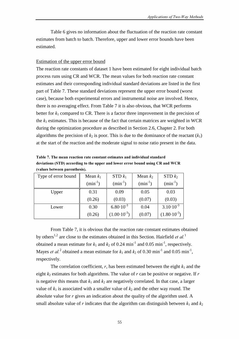
55

Table 6 gives no information about the fluctuation of the reaction rate constant

estimates from batch to batch. Therefore, upper and lower error bounds have been

estimated.

Estimation of the upper error bound

The reaction rate constants of dataset 1 have been estimated for eight individual batch

process runs using CR and WCR. The mean values for both reaction rate constant

estimates and their corresponding individual standard deviations are listed in the first

part of Table 7. These standard deviations represent the upper error bound (worst

case), because both experimental errors and instrumental noise are involved. Hence,

there is no averaging effect. From Table 7 it is also obvious, that WCR performs

better for �1 compared to CR. There is a factor three improvement in the precision of

the �1 estimates. This is because of the fact that certain matrices are weighted in WCR

during the optimization procedure as described in Section 2.6, Chapter 2. For both

algorithms the precision of �2 is poor. This is due to the dominance of the reactant (�1)

at the start of the reaction and the moderate signal to noise ratio present in the data.

��0��*��.�� .��+��

��+��-��%/�� ,��0��,��

-+��0��/�

Type of error bound Mean �1

(min-1)

STD �1

(min-1)

Mean �2

(min-1)

STD �2

(min-1)

Upper 0.31

(0.26)

0.09

(0.03)

0.05

(0.07)

0.03

(0.03)

Lower 0.30

(0.26)

6.80·10-3

(1.00·10-3)

0.04

(0.07)

3.10·10-3

(1.80·10-3)

From Table 7, it is obvious that the reaction rate constant estimates obtained

by others1,2 are close to the estimates obtained in this Section. Hairfield ��1

obtained a mean estimate for �1 and �2 of 0.24 min-1 and 0.05 min-1, respectively.

Mayes ��2 obtained a mean estimate for �1 and �2 of 0.30 min-1 and 0.05 min-1,

respectively.

The correlation coefficient, , has been estimated between the eight �1 and the

eight �2 estimates for both algorithms. The value of can be positive or negative. If

is negative this means that �1 and �2 are negatively correlated. In that case, a larger

value of �1 is associated with a smaller value of �2 and the other way round. The

absolute value for gives an indication about the quality of the algorithm used. A

small absolute value of indicates that the algorithm can distinguish between �1 and �2

��

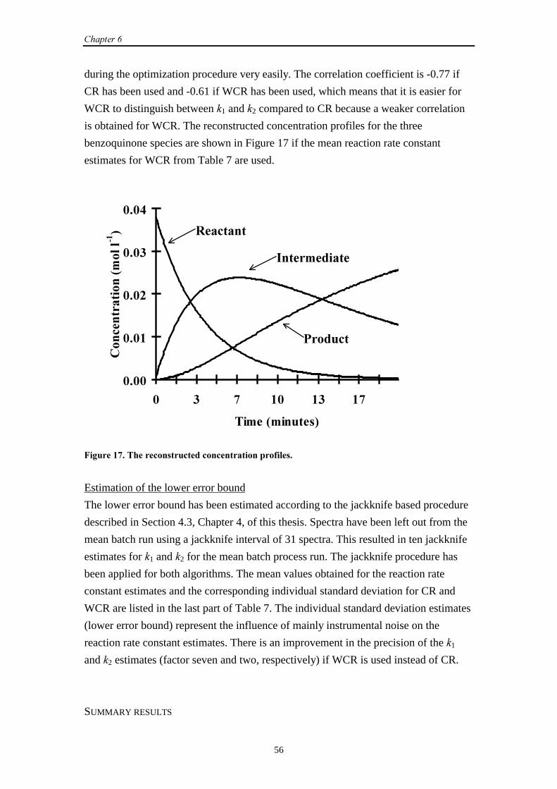
56

during the optimization procedure very easily. The correlation coefficient is -0.77 if

CR has been used and -0.61 if WCR has been used, which means that it is easier for

WCR to distinguish between �1 and �2 compared to CR because a weaker correlation

is obtained for WCR. The reconstructed concentration profiles for the three

benzoquinone species are shown in Figure 17 if the mean reaction rate constant

estimates for WCR from Table 7 are used.

'�''

'�'�

'�'�

'�'"

'�'!

' " * �' �" �*

��.��-.��/

�� -.��/

$�,��*��

Estimation of the lower error bound

The lower error bound has been estimated according to the jackknife based procedure

described in Section 4.3, Chapter 4, of this thesis. Spectra have been left out from the

mean batch run using a jackknife interval of 31 spectra. This resulted in ten jackknife

estimates for �1 and �2 for the mean batch process run. The jackknife procedure has

been applied for both algorithms. The mean values obtained for the reaction rate

constant estimates and the corresponding individual standard deviation for CR and

WCR are listed in the last part of Table 7. The individual standard deviation estimates

(lower error bound) represent the influence of mainly instrumental noise on the

reaction rate constant estimates. There is an improvement in the precision of the �1

and �2 estimates (factor seven and two, respectively) if WCR is used instead of CR.

SUMMARY RESULTS

��

��.��

5��

�� !"��#�$��

57

Using WCR, the mean estimated �1 value is 0.26 min-1 with an error between

1.00⋅10-3 min-1 (lower error bound) and 0.03 min-1 (upper error bound). With this

algorithm the mean estimated �2 value is 0.07 min-1 with an error between

1.80⋅10-3 min-1 (lower error bound) and 0.03 min-1 (upper error bound). These values

show that it is possible to estimate the reaction rate constants with good precision

even in case of high spectral overlap and a high noise level. For all �1 and �2 estimates,

too high �1 estimates tend to occur with too low �2 estimates and vice versa due to the

moderate correlation (-0.61) between both reaction rate constants.

��(��

Reaction rate constants have been estimated from dataset 1 using CR and WCR. This

dataset has been used as an example batch process to illustrate that the algorithms can

be applied successfully if there is a strong spectral overlap of the pure spectra of the

different reacting absorbing species and a high noise level are present in the data. An

advantage of the procedure described is the rapid estimation of the reaction constants.

Also upper and lower error bounds of the reaction rate constants can be estimated

which is very important for quality assessment. Simulations have shown that the

presented algorithms can be still applied successfully in case of an extreme overlap of

the spectra of the individual species involved in the considered process. From the

reaction rate constant estimates obtained from experimental and simulated data it can

be concluded that WCR performed the best with respect to the precision of reaction

rate constant estimates.

Because of the rapid estimation of the reaction rate constants from on-line

SW-NIR measurements, the use of the procedures presented can have many

applications in the field of obtaining information about batch processes and statistical

control of batch processes using fast on-line SW-NIR sensors. The expansion to more

complicated processes, e.g. batch polymerization processes is also possible.

�"�16�6��-�/

��%��

In Section 2.7 of Chapter 2 the use of constraints in CCR has been discussed in detail.

If pure spectra of some reacting absorbing species are known �� these can be

incorporated in CCR as a constraint resulting in constraint R or constraint RP. It is

expected that this will result in a better accuracy of kinetic parameter estimates

compared to methods which do not use this specific �� spectral information. In

this Section, constraint RP is implemented in CCR. Hence, the pure spectra of reactant

and product are both implemented in the CCR algorithm.

��

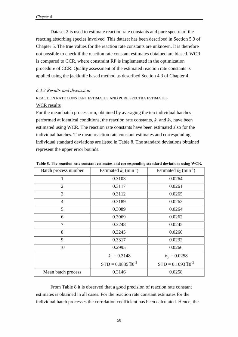
58

Dataset 2 is used to estimate reaction rate constants and pure spectra of the

reacting absorbing species involved. This dataset has been described in Section 5.3 of

Chapter 5. The true values for the reaction rate constants are unknown. It is therefore

not possible to check if the reaction rate constant estimates obtained are biased. WCR

is compared to CCR, where constraint RP is implemented in the optimization

procedure of CCR. Quality assessment of the estimated reaction rate constants is

applied using the jackknife based method as described Section 4.3 of Chapter 4.

��%��&��

REACTION RATE CONSTANT ESTIMATES AND PURE SPECTRA ESTIMATES

WCR results

For the mean batch process run, obtained by averaging the ten individual batches

performed at identical conditions, the reaction rate constants, �1 and �2, have been

estimated using WCR. The reaction rate constants have been estimated also for the

individual batches. The mean reaction rate constant estimates and corresponding

individual standard deviations are listed in Table 8. The standard deviations obtained

represent the upper error bounds.

��0��(�� .�� ,��+��,��

Batch process number Estimated �1 (min-1) Estimated �2 (min-1)

1 0.3103 0.0264

2 0.3117 0.0261

3 0.3112 0.0265

4 0.3189 0.0262

5 0.3089 0.0264

6 0.3069 0.0262

7 0.3248 0.0245

8 0.3245 0.0260

9 0.3317 0.0232

10 0.2995 0.0266

�1 = 0.3148

STD = 0.9835⋅10-2

2� = 0.0258

STD = 0.1093⋅10-2

Mean batch process 0.3146 0.0258

From Table 8 it is observed that a good precision of reaction rate constant

estimates is obtained in all cases. For the reaction rate constant estimates for the

individual batch processes the correlation coefficient has been calculated. Hence, the

�� !"��#�$��

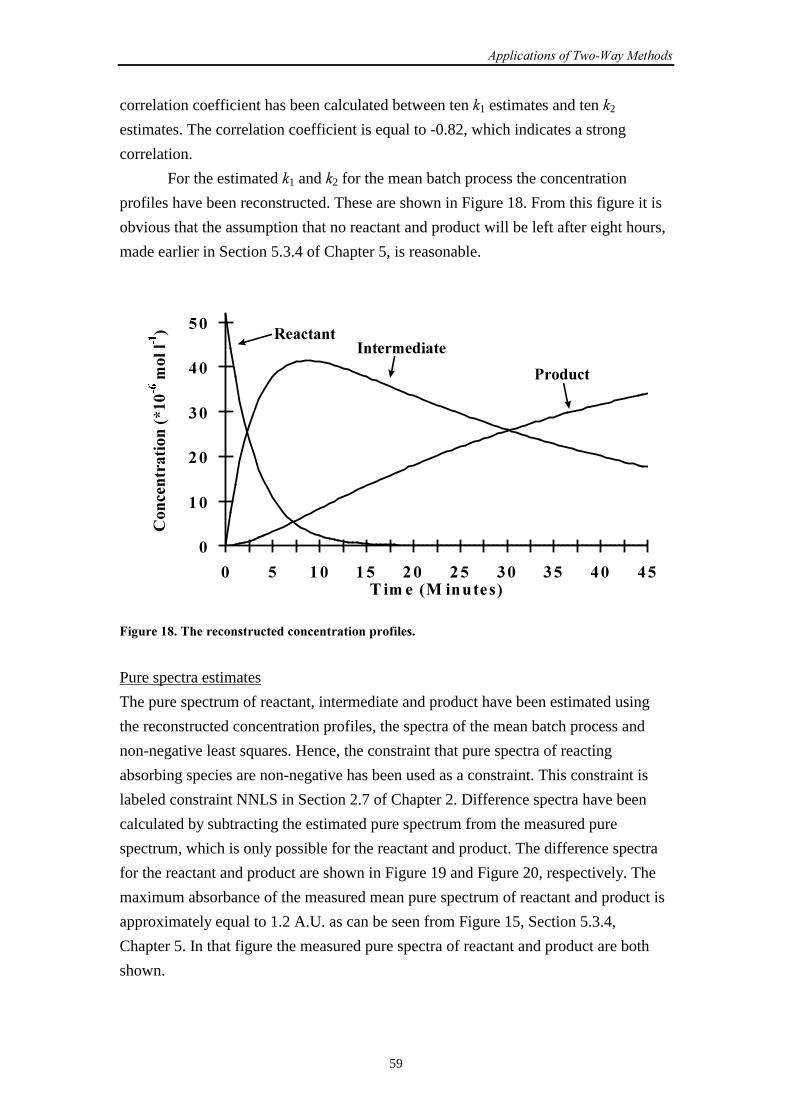
59

correlation coefficient has been calculated between ten �1 estimates and ten �2

estimates. The correlation coefficient is equal to -0.82, which indicates a strong

correlation.

For the estimated �1 and �2 for the mean batch process the concentration

profiles have been reconstructed. These are shown in Figure 18. From this figure it is

obvious that the assumption that no reactant and product will be left after eight hours,

made earlier in Section 5.3.4 of Chapter 5, is reasonable.

�� .��

5��

'

�'

�'

"'

!'

)'

' ) �' �) �' �) "' ") !' !)� �. ��-� ��/

�� -7�'�

�

�.��

�

/

$�,��(��

Pure spectra estimates

The pure spectrum of reactant, intermediate and product have been estimated using

the reconstructed concentration profiles, the spectra of the mean batch process and

non-negative least squares. Hence, the constraint that pure spectra of reacting

absorbing species are non-negative has been used as a constraint. This constraint is

labeled constraint NNLS in Section 2.7 of Chapter 2. Difference spectra have been

calculated by subtracting the estimated pure spectrum from the measured pure

spectrum, which is only possible for the reactant and product. The difference spectra

for the reactant and product are shown in Figure 19 and Figure 20, respectively. The

maximum absorbance of the measured mean pure spectrum of reactant and product is

approximately equal to 1.2 A.U. as can be seen from Figure 15, Section 5.3.4,

Chapter 5. In that figure the measured pure spectra of reactant and product are both

shown.

��

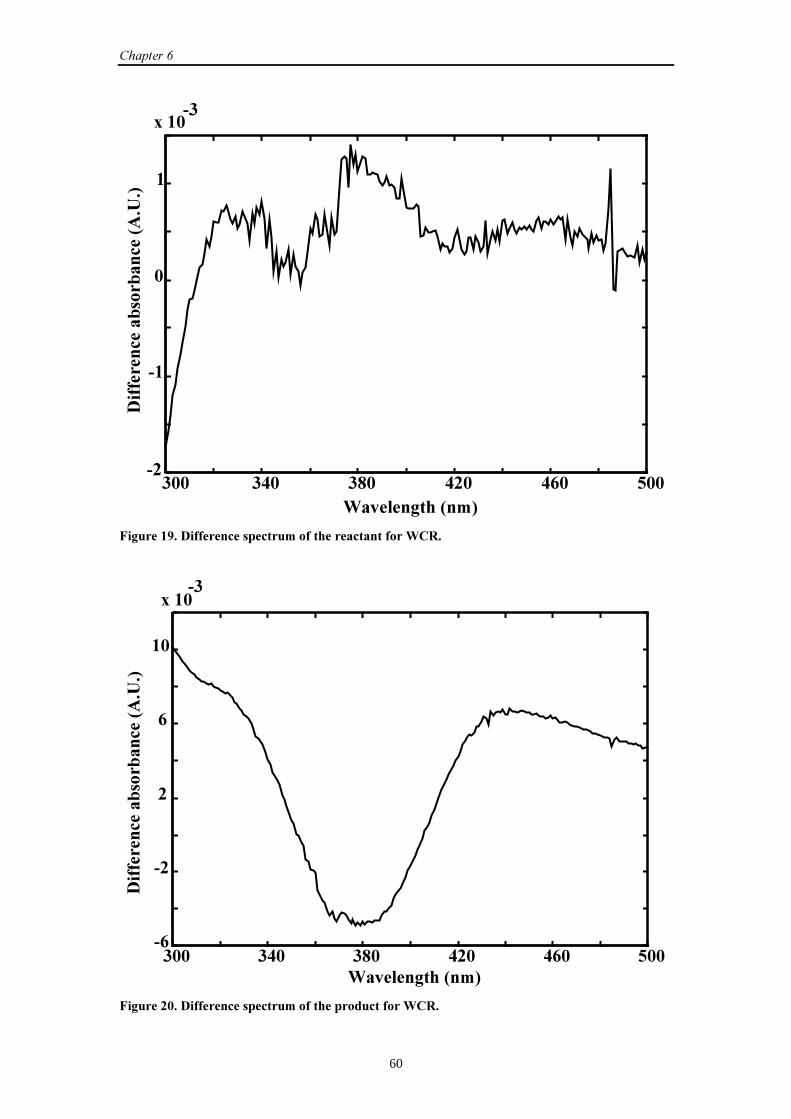
60

"'' "!' "(' !�' !' )''��

��

'

�

4��'�"

��+��,��-�./

%�� 0��0�� -�1�/

$�,��#��%�� .��

"'' "!' "(' !�' !' )''�

��

�

�'

4��'�"

��+��,��-�./

%�� 0��0�� -�1�/

$�,��'��%�� .��

�� !"��#�$��

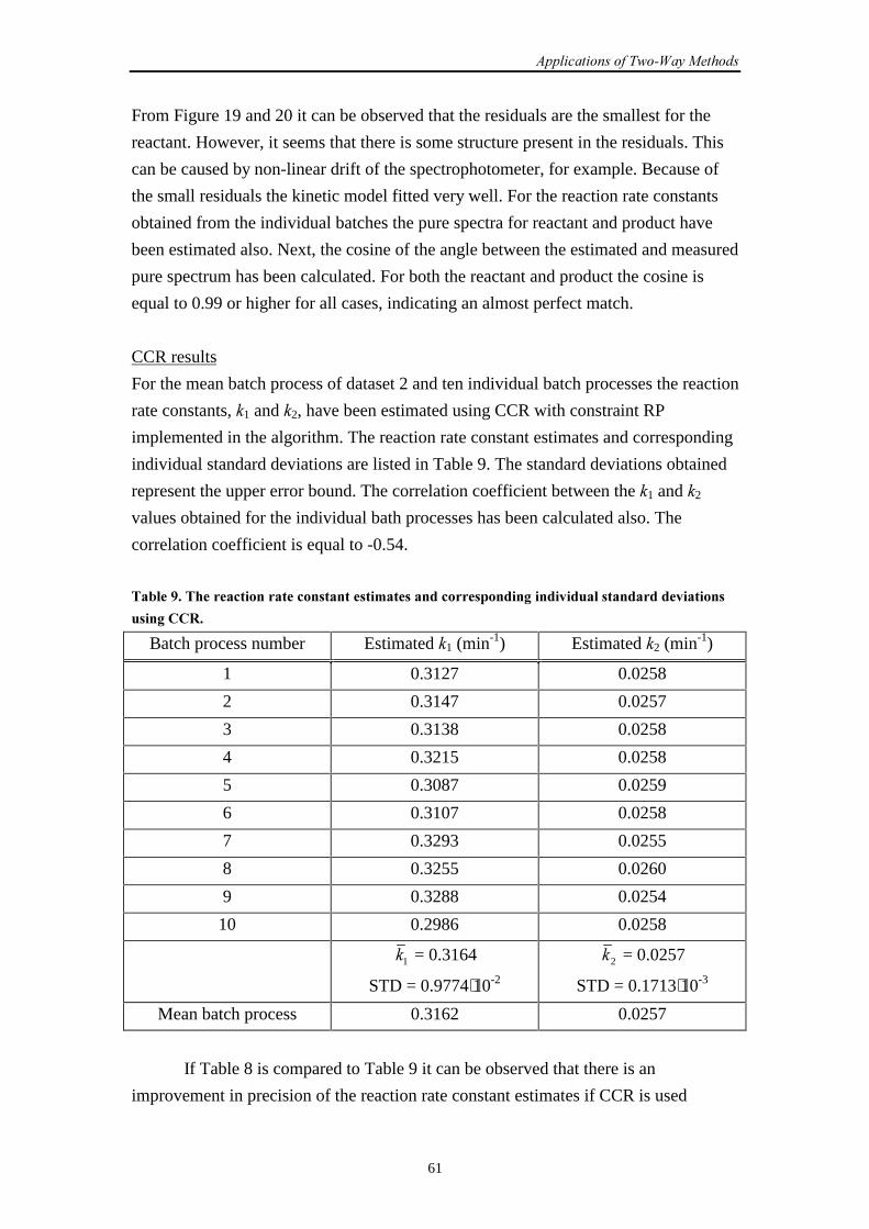
61

From Figure 19 and 20 it can be observed that the residuals are the smallest for the

reactant. However, it seems that there is some structure present in the residuals. This

can be caused by non-linear drift of the spectrophotometer, for example. Because of

the small residuals the kinetic model fitted very well. For the reaction rate constants

obtained from the individual batches the pure spectra for reactant and product have

been estimated also. Next, the cosine of the angle between the estimated and measured

pure spectrum has been calculated. For both the reactant and product the cosine is

equal to 0.99 or higher for all cases, indicating an almost perfect match.

CCR results

For the mean batch process of dataset 2 and ten individual batch processes the reaction

rate constants, �1 and �2, have been estimated using CCR with constraint RP

implemented in the algorithm. The reaction rate constant estimates and corresponding

individual standard deviations are listed in Table 9. The standard deviations obtained

represent the upper error bound. The correlation coefficient between the �1 and �2

values obtained for the individual bath processes has been calculated also. The

correlation coefficient is equal to -0.54.

��0��#�� .�� ,��+��+��

��,��

Batch process number Estimated �1 (min-1) Estimated �2 (min-1)

1 0.3127 0.0258

2 0.3147 0.0257

3 0.3138 0.0258

4 0.3215 0.0258

5 0.3087 0.0259

6 0.3107 0.0258

7 0.3293 0.0255

8 0.3255 0.0260

9 0.3288 0.0254

10 0.2986 0.0258

�1 = 0.3164

STD = 0.9774⋅10-2

2� = 0.0257

STD = 0.1713⋅10-3

Mean batch process 0.3162 0.0257

If Table 8 is compared to Table 9 it can be observed that there is an

improvement in precision of the reaction rate constant estimates if CCR is used

��

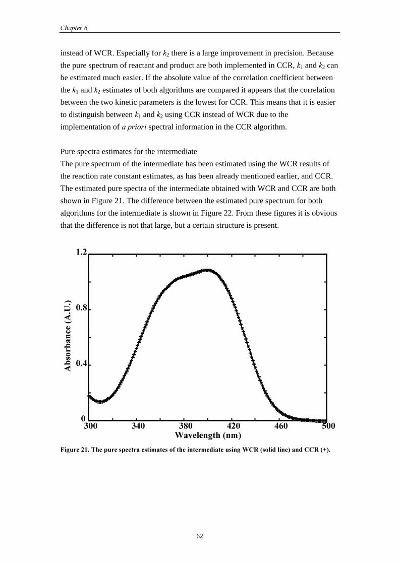
62

instead of WCR. Especially for �2 there is a large improvement in precision. Because

the pure spectrum of reactant and product are both implemented in CCR, �1 and �2 can

be estimated much easier. If the absolute value of the correlation coefficient between

the �1 and �2 estimates of both algorithms are compared it appears that the correlation

between the two kinetic parameters is the lowest for CCR. This means that it is easier

to distinguish between �1 and �2 using CCR instead of WCR due to the

implementation of �� spectral information in the CCR algorithm.

Pure spectra estimates for the intermediate

The pure spectrum of the intermediate has been estimated using the WCR results of

the reaction rate constant estimates, as has been already mentioned earlier, and CCR.

The estimated pure spectra of the intermediate obtained with WCR and CCR are both

shown in Figure 21. The difference between the estimated pure spectrum for both

algorithms for the intermediate is shown in Figure 22. From these figures it is obvious

that the difference is not that large, but a certain structure is present.

"'' "!' "(' !�' !' )'''

'�!

'�(

��

��+��,��-�./

0��0�� -�1�/

$�,�� .��.��,�� -��/�� -8/�

�� !"��#�$��

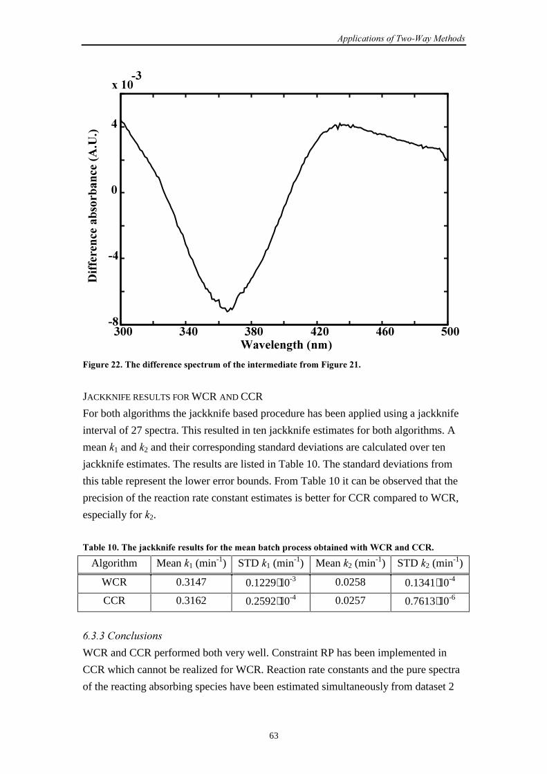
63

"'' "!' "(' !�' !' )''�(

�!

'

!

4��'�"

��+��,��-�./

%�� 0��0�� -�1�/

$�,�� .��.��.�$�,��

JACKKNIFE RESULTS FOR WCR AND CCR

For both algorithms the jackknife based procedure has been applied using a jackknife

interval of 27 spectra. This resulted in ten jackknife estimates for both algorithms. A

mean �1 and �2 and their corresponding standard deviations are calculated over ten

jackknife estimates. The results are listed in Table 10. The standard deviations from

this table represent the lower error bounds. From Table 10 it can be observed that the

precision of the reaction rate constant estimates is better for CCR compared to WCR,

especially for �2.

��0��'��9� ::��.��0�� 0��

Algorithm Mean �1 (min-1) STD �1 (min-1) Mean �2 (min-1) STD �2 (min-1)

WCR 0.3147 0.1229⋅10-3 0.0258 0.1341⋅10-4

CCR 0.3162 0.2592⋅10-4 0.0257 0.7613⋅10-6

��%�%��

WCR and CCR performed both very well. Constraint RP has been implemented in

CCR which cannot be realized for WCR. Reaction rate constants and the pure spectra

of the reacting absorbing species have been estimated simultaneously from dataset 2

��

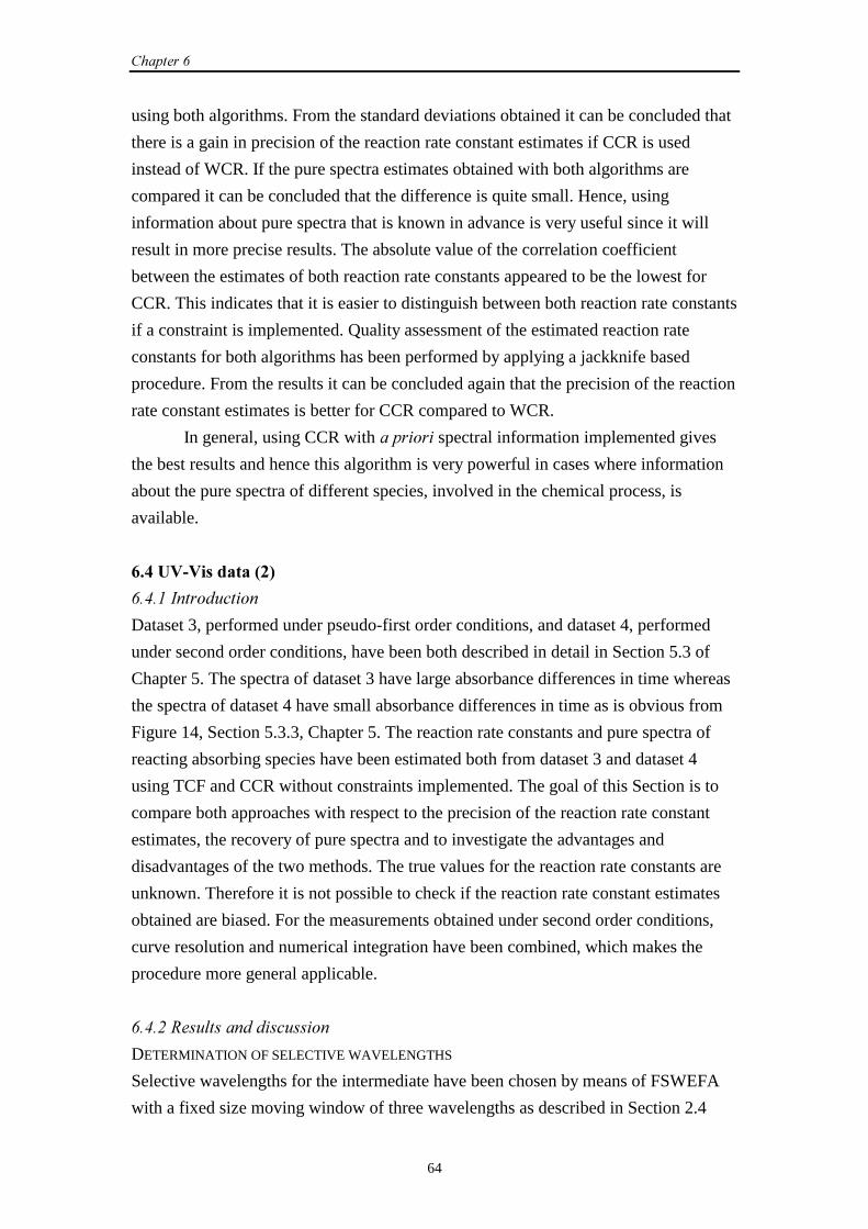
64

using both algorithms. From the standard deviations obtained it can be concluded that

there is a gain in precision of the reaction rate constant estimates if CCR is used

instead of WCR. If the pure spectra estimates obtained with both algorithms are

compared it can be concluded that the difference is quite small. Hence, using

information about pure spectra that is known in advance is very useful since it will

result in more precise results. The absolute value of the correlation coefficient

between the estimates of both reaction rate constants appeared to be the lowest for

CCR. This indicates that it is easier to distinguish between both reaction rate constants

if a constraint is implemented. Quality assessment of the estimated reaction rate

constants for both algorithms has been performed by applying a jackknife based

procedure. From the results it can be concluded again that the precision of the reaction

rate constant estimates is better for CCR compared to WCR.

In general, using CCR with �� spectral information implemented gives

the best results and hence this algorithm is very powerful in cases where information

about the pure spectra of different species, involved in the chemical process, is

available.

�!�16�6��-�/

��(��

Dataset 3, performed under pseudo-first order conditions, and dataset 4, performed

under second order conditions, have been both described in detail in Section 5.3 of

Chapter 5. The spectra of dataset 3 have large absorbance differences in time whereas

the spectra of dataset 4 have small absorbance differences in time as is obvious from

Figure 14, Section 5.3.3, Chapter 5. The reaction rate constants and pure spectra of

reacting absorbing species have been estimated both from dataset 3 and dataset 4

using TCF and CCR without constraints implemented. The goal of this Section is to

compare both approaches with respect to the precision of the reaction rate constant

estimates, the recovery of pure spectra and to investigate the advantages and

disadvantages of the two methods. The true values for the reaction rate constants are

unknown. Therefore it is not possible to check if the reaction rate constant estimates

obtained are biased. For the measurements obtained under second order conditions,

curve resolution and numerical integration have been combined, which makes the

procedure more general applicable.

��(��&��

DETERMINATION OF SELECTIVE WAVELENGTHS

Selective wavelengths for the intermediate have been chosen by means of FSWEFA

with a fixed size moving window of three wavelengths as described in Section 2.4

�� !"��#�$��

65

from Chapter 2. In Figure 23 the FSWEFA plots (log (singular value) as a function of

the position of the window) are shown for one individual batch process run under

pseudo-first order conditions and one individual batch process run obtained under

second order conditions. FSWEFA plots obtained for other individual batches are

comparable.

"'' "!' "(' !�' !' )''��'

�

��

�

5��

��,�-��,��+��/

"'' "!' "(' !�' !' )''��'

�

��

�

��,�-��,��+��/

;�5�� <;��

5��

=� ��:�>��=� ��:�>��

$�,��"��5��,�-��,��+��/�+��$��?$��

In Figure 23, the position of the window equal to 301 means wavelength range

300-302 nm, the position of the window equal to 340 corresponds to 339-341 nm,

etc… If Figure 23 is examined critically it can be observed that the local rank case of

interest (local rank equals 1), is at position number 444. This corresponds to the

wavelength range 443-445 nm. Hence, at this window absorbance differences are

mainly caused by one species. It is known that the pure spectra of reactant and product

have no absorbances in the wavelength range 443-445 nm (see Figure 15,

Section 5.3.4, Chapter 5). Therefore it is reasonable to assume that the absorbances at

this wavelength range are mainly caused by the intermediate.

REACTION RATE CONSTANT ESTIMATES

In this Section, the focus will be mainly on the precision of the reaction rate constant

estimates. TCF and CCR have both been applied to the pseudo-first order dataset

(dataset 3) and the second order dataset (dataset 4). The reaction rate constant

estimates for every individual batch for the two methods are shown in Figure 24.

��

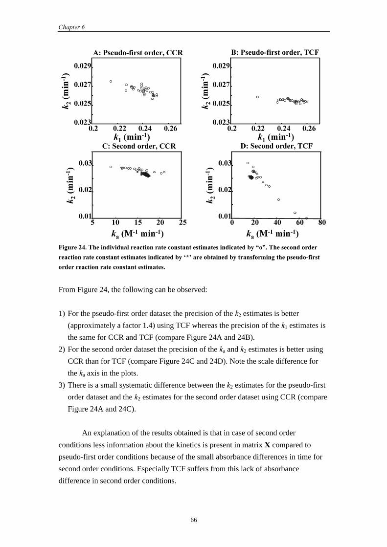
66

'�� '�� '��! '��'�'�"

'�'�)

'�'�*

'�'�#

'�� '�� '��! '��'�'�"

'�'�)

'�'�*

'�'�#� ��-.��/

��-.��/

� ��-.��/

��-.��/

��-��.��/

� ��-.��/

� ��-.��/

��-��.��/

;�5��3��

�;�� 3��

<;�5��3��$

%;�� 3��$

) �' �) �' �)'�'�

'�'�

'�'"

' �' !' ' (''�'�

'�'�

'�'"

$�,��!��+�� .�� 0��@�A��

�� .�� 0��B7C��0��0��.��,��

�� .��

From Figure 24, the following can be observed:

1) For the pseudo-first order dataset the precision of the �2 estimates is better

(approximately a factor 1.4) using TCF whereas the precision of the �1 estimates is

the same for CCR and TCF (compare Figure 24A and 24B).

2) For the second order dataset the precision of the �a and �2 estimates is better using

CCR than for TCF (compare Figure 24C and 24D). Note the scale difference for

the �a axis in the plots.

3) There is a small systematic difference between the �2 estimates for the pseudo-first

order dataset and the �2 estimates for the second order dataset using CCR (compare

Figure 24A and 24C).

An explanation of the results obtained is that in case of second order

conditions less information about the kinetics is present in matrix & compared to

pseudo-first order conditions because of the small absorbance differences in time for

second order conditions. Especially TCF suffers from this lack of absorbance

difference in second order conditions.

�� !"��#�$��

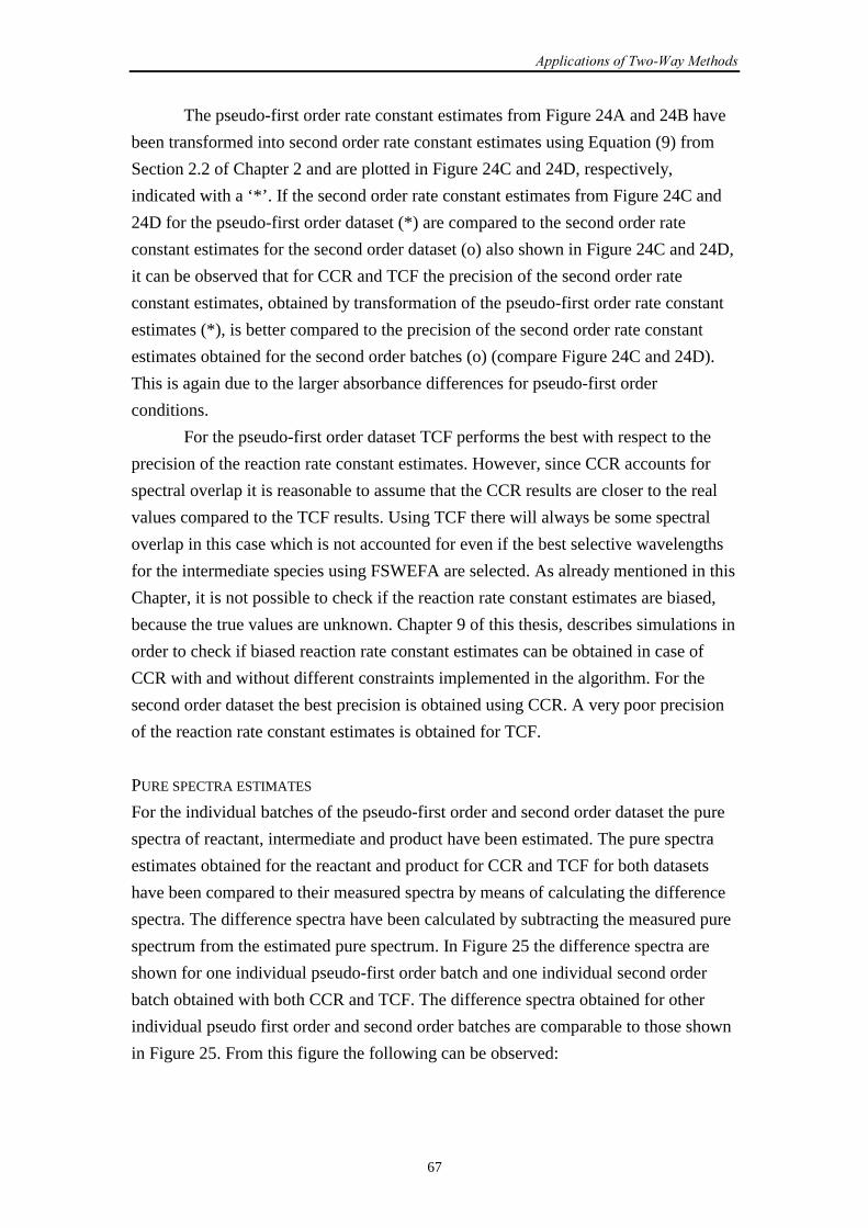
67

The pseudo-first order rate constant estimates from Figure 24A and 24B have

been transformed into second order rate constant estimates using Equation (9) from

Section 2.2 of Chapter 2 and are plotted in Figure 24C and 24D, respectively,

indicated with a ‘*’. If the second order rate constant estimates from Figure 24C and

24D for the pseudo-first order dataset (*) are compared to the second order rate

constant estimates for the second order dataset (o) also shown in Figure 24C and 24D,

it can be observed that for CCR and TCF the precision of the second order rate

constant estimates, obtained by transformation of the pseudo-first order rate constant

estimates (*), is better compared to the precision of the second order rate constant

estimates obtained for the second order batches (o) (compare Figure 24C and 24D).

This is again due to the larger absorbance differences for pseudo-first order

conditions.

For the pseudo-first order dataset TCF performs the best with respect to the

precision of the reaction rate constant estimates. However, since CCR accounts for

spectral overlap it is reasonable to assume that the CCR results are closer to the real

values compared to the TCF results. Using TCF there will always be some spectral

overlap in this case which is not accounted for even if the best selective wavelengths

for the intermediate species using FSWEFA are selected. As already mentioned in this

Chapter, it is not possible to check if the reaction rate constant estimates are biased,

because the true values are unknown. Chapter 9 of this thesis, describes simulations in

order to check if biased reaction rate constant estimates can be obtained in case of

CCR with and without different constraints implemented in the algorithm. For the

second order dataset the best precision is obtained using CCR. A very poor precision

of the reaction rate constant estimates is obtained for TCF.

PURE SPECTRA ESTIMATES

For the individual batches of the pseudo-first order and second order dataset the pure

spectra of reactant, intermediate and product have been estimated. The pure spectra

estimates obtained for the reactant and product for CCR and TCF for both datasets

have been compared to their measured spectra by means of calculating the difference

spectra. The difference spectra have been calculated by subtracting the measured pure

spectrum from the estimated pure spectrum. In Figure 25 the difference spectra are

shown for one individual pseudo-first order batch and one individual second order

batch obtained with both CCR and TCF. The difference spectra obtained for other

individual pseudo first order and second order batches are comparable to those shown

in Figure 25. From this figure the following can be observed:

��

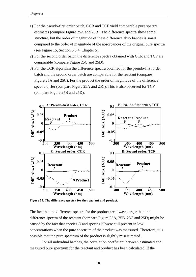
68

1) For the pseudo-first order batch, CCR and TCF yield comparable pure spectra

estimates (compare Figure 25A and 25B). The difference spectra show some

structure, but the order of magnitude of these difference absorbances is small

compared to the order of magnitude of the absorbances of the original pure spectra

(see Figure 15, Section 5.3.4, Chapter 5).

2) For the second order batch the difference spectra obtained with CCR and TCF are

comparable (compare Figure 25C and 25D).

3) For the CCR algorithm the difference spectra obtained for the pseudo-first order

batch and the second order batch are comparable for the reactant (compare

Figure 25A and 25C). For the product the order of magnitude of the difference

spectra differ (compare Figure 25A and 25C). This is also observed for TCF

(compare Figure 25B and 25D).

"'' )''")' !'' !)'�'��

�'�')

'

'�')

'��

"'' ")' !'' !)' )''�'��

�'�')

'

'�')

'��

"'' ")' !'' !)' )''�'��

�'�')

'

'�')

'��

"'' ")' !'' !)' )''�'��

�'�')

'

'�')

'��

%��0��-�1�/

%��0��-�1�/

%��0��-�1�/

%��0��-�1�/

;�5��3��

�;�� 3��

<;�5��3��$

%;�� 3��$

�� 5��

�� 5��

��

5��

5��

��+��,��-�./

��+��,��-�./

��+��,��-�./

��+��,��-�./

$�,��)��

The fact that the difference spectra for the product are always larger than the

difference spectra of the reactant (compare Figure 25A, 25B, 25C and 25D) might be

caused by the fact that species � and species � were still present in low

concentrations when the pure spectrum of the product was measured. Therefore, it is

possible that the pure spectrum of the product is slightly misestimated.

For all individual batches, the correlation coefficient between estimated and

measured pure spectrum for the reactant and product has been calculated. If the

�� !"��#�$��

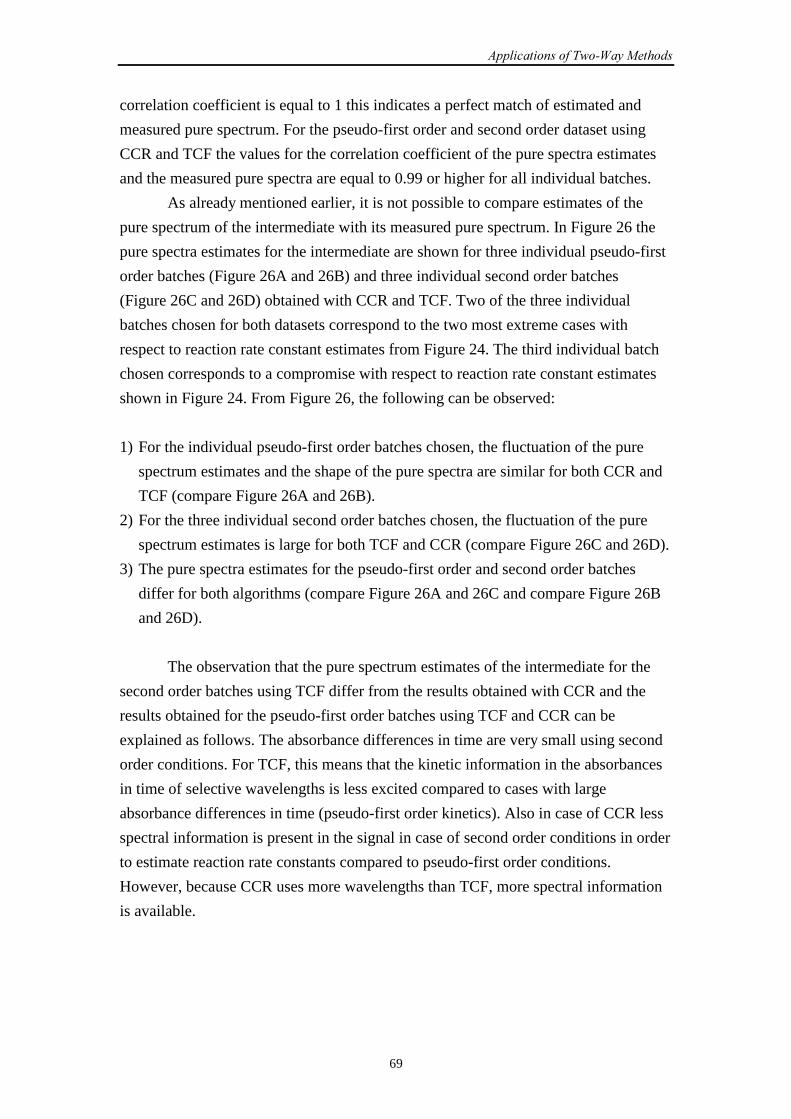
69

correlation coefficient is equal to 1 this indicates a perfect match of estimated and

measured pure spectrum. For the pseudo-first order and second order dataset using

CCR and TCF the values for the correlation coefficient of the pure spectra estimates

and the measured pure spectra are equal to 0.99 or higher for all individual batches.

As already mentioned earlier, it is not possible to compare estimates of the

pure spectrum of the intermediate with its measured pure spectrum. In Figure 26 the

pure spectra estimates for the intermediate are shown for three individual pseudo-first

order batches (Figure 26A and 26B) and three individual second order batches

(Figure 26C and 26D) obtained with CCR and TCF. Two of the three individual

batches chosen for both datasets correspond to the two most extreme cases with

respect to reaction rate constant estimates from Figure 24. The third individual batch

chosen corresponds to a compromise with respect to reaction rate constant estimates

shown in Figure 24. From Figure 26, the following can be observed:

1) For the individual pseudo-first order batches chosen, the fluctuation of the pure

spectrum estimates and the shape of the pure spectra are similar for both CCR and

TCF (compare Figure 26A and 26B).

2) For the three individual second order batches chosen, the fluctuation of the pure

spectrum estimates is large for both TCF and CCR (compare Figure 26C and 26D).

3) The pure spectra estimates for the pseudo-first order and second order batches

differ for both algorithms (compare Figure 26A and 26C and compare Figure 26B

and 26D).

The observation that the pure spectrum estimates of the intermediate for the

second order batches using TCF differ from the results obtained with CCR and the

results obtained for the pseudo-first order batches using TCF and CCR can be

explained as follows. The absorbance differences in time are very small using second

order conditions. For TCF, this means that the kinetic information in the absorbances

in time of selective wavelengths is less excited compared to cases with large

absorbance differences in time (pseudo-first order kinetics). Also in case of CCR less

spectral information is present in the signal in case of second order conditions in order

to estimate reaction rate constants compared to pseudo-first order conditions.

However, because CCR uses more wavelengths than TCF, more spectral information

is available.

��

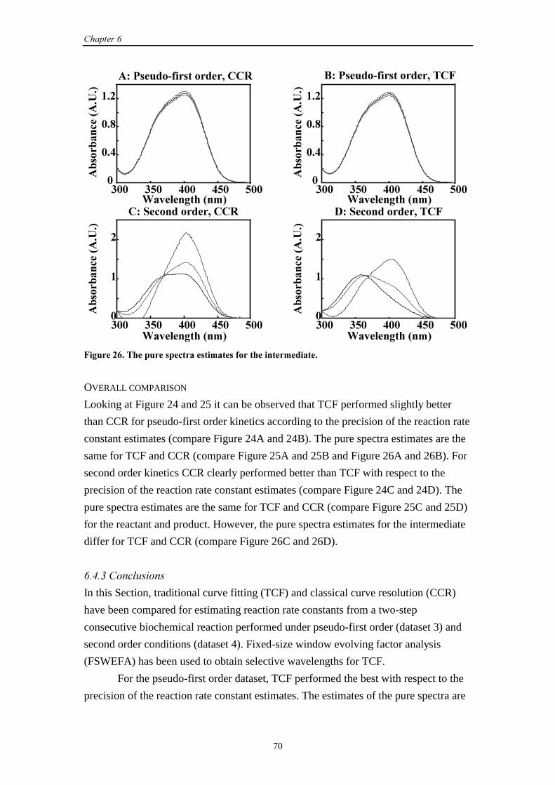
70

"'' ")' !'' !)' )'''

'�!

'�(

��

"'' ")' !'' !)' )'''

'�!

'�(

��

"'' ")' !'' !)' )'''

�

�

"'' ")' !'' !)' )'''

�

�

0��0�� -�1�/

;�5��3�� <;�5��3��$

0��0�� -�1�/

��+��,��-�./ ��+��,��-�./�;�� 3�� %;�� 3��$

0��0�� -�1�/

0��0�� -�1�/

��+��,��-�./ ��+��,��-�./

$�,�� .��.��

OVERALL COMPARISON

Looking at Figure 24 and 25 it can be observed that TCF performed slightly better

than CCR for pseudo-first order kinetics according to the precision of the reaction rate

constant estimates (compare Figure 24A and 24B). The pure spectra estimates are the

same for TCF and CCR (compare Figure 25A and 25B and Figure 26A and 26B). For

second order kinetics CCR clearly performed better than TCF with respect to the

precision of the reaction rate constant estimates (compare Figure 24C and 24D). The

pure spectra estimates are the same for TCF and CCR (compare Figure 25C and 25D)

for the reactant and product. However, the pure spectra estimates for the intermediate

differ for TCF and CCR (compare Figure 26C and 26D).

��(�%��

In this Section, traditional curve fitting (TCF) and classical curve resolution (CCR)

have been compared for estimating reaction rate constants from a two-step

consecutive biochemical reaction performed under pseudo-first order (dataset 3) and

second order conditions (dataset 4). Fixed-size window evolving factor analysis

(FSWEFA) has been used to obtain selective wavelengths for TCF.

For the pseudo-first order dataset, TCF performed the best with respect to the

precision of the reaction rate constant estimates. The estimates of the pure spectra are

�� !"��#�$��

71

similar for TCF and CCR. For the second order dataset CCR performed the best with

respect to the precision of the reaction rate constant estimates. A possible reason for

the relatively poor performance of the TCF algorithm with respect to the precision of

the reaction rate constant estimates for the second order dataset, are the small

absorbance differences in time in the signal in order to estimate the reaction rate

constants. The estimates of the pure spectra differed for TCF and CCR.

In general, it can be concluded that both CCR and TCF perform very well in

case of spectral data where the absorbance differences in time are large and a good

selective window exists. In that case TCF is preferred because it is simple and fast

compared to CCR. These properties make TCF very suitable for on-line monitoring

reaction rate constants and process control. In more complicated situations, for

example, in case of small absorbance differences in time or severe spectral overlap (no

availability of selective wavelengths) CCR performs better. In case of doubt CCR is

always preferred.

�)�D��

In this Chapter, results have been presented using different two-way methods for

estimating reaction rate constants. Four different experimental datasets and simulated

datasets have been used to test the performance of the algorithms. The following

general conclusions can be formulated from the results:

1) WCR leads to a better precision of reaction rate constant estimates compared to

CR.

2) If constraint RP is implemented in CCR this leads to a better precision of reaction

rate constant estimates compared to WCR.

3) CCR is applicable for �-th order kinetics.

4) If there are large absorbance differences in time present (high selectivity in the time

direction) in the dataset (in this case this holds for pseudo-first order kinetics), TCF

is applicable and is superior to CCR without �� spectral information

implemented in the algorithm.

5) If there are small absorbance differences in time present (low selectivity in the time

direction) in the dataset (in this case this holds for second order kinetics), TCF

leads to a poor precision of reaction rate constant estimates compared to CCR

without constraints implemented.

��

72

�� 1. Hairfield EM, Moomaw EW, Tamburri RA, Vigil RA.�‘The epoxidation of

2,5-di-tert-butyl-1,4-benzoquinone’. �� , 1985; �: 175-177.


with shortwave near-infrared spectroscopy’, in )�� &�� #*�+��,��,��-��

.��"��/��#��)�&�� , ed. by Hildrum KI, Isaksson T, Naes T, Tandberg A.


73

��

��

��

In this Chapter,i the results of the application of the generalized rank annihilation

method (GRAM) and the generalized rank annihilation method-Levenberg-Marquardt-

parallel factor analysis (GRAM-LM-PAR) method to dataset 1 and dataset 2 are

presented. Dataset 1 and dataset 2 have been described in Section 5.2 and Section 5.3,

respectively, of Chapter 5. The theory of the three-way methods has been described in

Section 3.4 and Section 3.5 of Chapter 3. However, in this Chapter the application of

the three-way methods the trilinear decomposition method (TLD) and the trilinear

decomposition method-Levenberg-Marquardt-parallel factor analysis (TLD-LM-PAR)

method are not presented. This is postponed until Chapter 8, where also a comparison

is made between the performance of two-way and three-way methods.

��

��

In this Section, simulations based on a two-step consecutive reaction are used to show

that GRAM and GRAM-LM-PAR, described in Section 3.4 and Section 3.5 of

Chapter 3, can be applied to estimate reaction rate constants in case of extreme

spectral overlap of different species involved in the reacting system. The performance

of both algorithms is also tested on the spectra of dataset 1 (SW-NIR data) described

in Section 5.2 of Chapter 5. Quality assessment of the estimated reaction rate

constants is performed using a jackknife based method (see Section 4.3, Chapter 4).

i This Chapter is based on the following papers:

� Bijlsma S, Louwerse DJ, Windig W, Smilde AK. ‘Rapid estimation of rate constants using on-line

SW-NIR and trilinear models’. �� , 1998; !: 339-355.

� Bijlsma S, Louwerse DJ, Smilde AK. ‘Estimating rate constants and pure UV-Vis spectra of a two-step

reaction using trilinear models’. �� , 1999; � : 311-329.

��

74

��

The set-up of the simulations was identical to the set-up described in Section 6.2.2 of

Chapter 6. Simulations have been performed using GRAM and GRAM-LM-PAR

under different simulated conditions: different amounts of peak overlap and different

noise levels. The true values for the reaction rate constants were always 0.30 min-1 and

0.05 min-1 for �1 and �2, respectively. The time shift parameter � was equal to 1

spectrum and the values of the elements in the column with constants, added to

datamatrix " (soft constraint), were equal to 100000.

��

SIMULATIONS

The mean reaction rate constant estimates for �1 and �2 using GRAM and

GRAM-LM-PAR are listed in Table 11 for two different noise levels (1% and 4%)

and four different situations of spectral overlap of the pure spectra of the reacting

absorbing species. From Table 11 the following can be observed:

1) A higher noise level results in a poorer precision for both �1 and �2 estimates.

2) If the noise level is kept constant and the spectral overlap becomes stronger, a

poorer precision is obtained for both reaction rate constants.

3) If GRAM-LM-PAR is used instead of GRAM, the precision of the reaction rate

constant estimates is improved for both kinetic parameters. Moreover, the mean

estimated values are closer to the true values.

If the noise level is increased to higher values than 4%, many individual �1

estimates are equal to the corresponding individual �2 estimates. This is illustrated

using the following simulations. For a fixed spectral overlap (�PD[�8 = 900 nm,

�PD[�: = 950 nm and �PD[�< = 1000 nm) 100 SW-NIR datasets have been simulated for

two different noise levels (10% and 15%). The kinetic parameters have been estimated

using GRAM. For a noise level of 10% in five cases �1 equals �2. For a noise level of

15% in 27 cases �1 equals �2. A possible explanation for this phenomenon is that if the

noise level is very high it is very hard to distinguish between the two exponential

functions � N W− 1 and WN� 2− . If this noise effect occurs this can easily be detected from the

� matrix, because the first two columns will be equal and hence �1 equals �2.

The choice of the column with constants appeared to be very important. If the

constants are equal to 1 the third column of and � (�3 and 3, respectively) are not

always constant. If the column with constants is much larger than the signals present

in ", �3 and 3 are forced to be constant. Therefore the column with constants was

�� !�"�#��

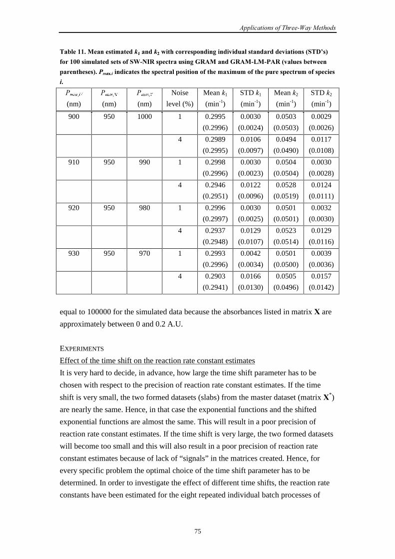
75

��#��$��%�� &��'��'��(��)*�+

��,,��$�� &�-��-��.��/��('��#��%��

��+��PD[�L�� $�0�$�$�� $��

��

�PD[,8(nm)

�PD[,:(nm)

�PD[,<(nm)

Noise

level (%)

Mean �1

(min-1)

STD �1

(min-1)

Mean �2

(min-1)

STD �2

(min-1)

900 950 1000 1 0.2995

(0.2996)

0.0030

(0.0024)

0.0503

(0.0503)

0.0029

(0.0026)

4 0.2989

(0.2995)

0.0106

(0.0097)

0.0494

(0.0490)

0.0117

(0.0108)

910 950 990 1 0.2998

(0.2996)

0.0030

(0.0023)

0.0504

(0.0504)

0.0030

(0.0028)

4 0.2946

(0.2951)

0.0122

(0.0096)

0.0528

(0.0519)

0.0124

(0.0111)

920 950 980 1 0.2996

(0.2997)

0.0030

(0.0025)

0.0501

(0.0501)

0.0032

(0.0030)

4 0.2937

(0.2948)

0.0129

(0.0107)

0.0523

(0.0514)

0.0129

(0.0116)

930 950 970 1 0.2993

(0.2996)

0.0042

(0.0034)

0.0501

(0.0500)

0.0039

(0.0036)

4 0.2903

(0.2941)

0.0166

(0.0130)

0.0505

(0.0496)

0.0157

(0.0142)

equal to 100000 for the simulated data because the absorbances listed in matrix " are

approximately between 0 and 0.2 A.U.

EXPERIMENTS

Effect of the time shift on the reaction rate constant estimates

It is very hard to decide, in advance, how large the time shift parameter has to be

chosen with respect to the precision of reaction rate constant estimates. If the time

shift is very small, the two formed datasets (slabs) from the master dataset (matrix "*)

are nearly the same. Hence, in that case the exponential functions and the shifted

exponential functions are almost the same. This will result in a poor precision of

reaction rate constant estimates. If the time shift is very large, the two formed datasets

will become too small and this will also result in a poor precision of reaction rate

constant estimates because of lack of “signals” in the matrices created. Hence, for

every specific problem the optimal choice of the time shift parameter has to be

determined. In order to investigate the effect of different time shifts, the reaction rate

constants have been estimated for the eight repeated individual batch processes of

��

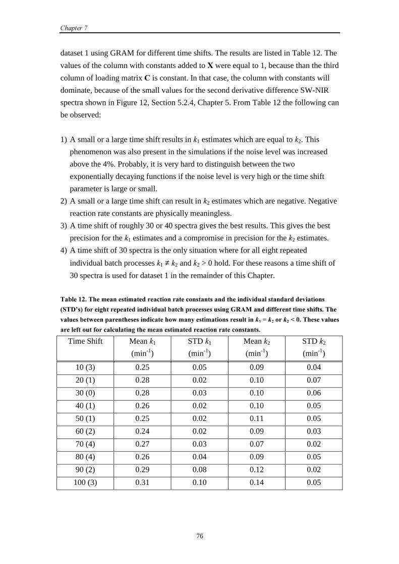
76

dataset 1 using GRAM for different time shifts. The results are listed in Table 12. The

values of the column with constants added to " were equal to 1, because than the third

column of loading matrix � is constant. In that case, the column with constants will

dominate, because of the small values for the second derivative difference SW-NIR

spectra shown in Figure 12, Section 5.2.4, Chapter 5. From Table 12 the following can

be observed:

1) A small or a large time shift results in �1 estimates which are equal to �2. This

phenomenon was also present in the simulations if the noise level was increased

above the 4%. Probably, it is very hard to distinguish between the two

exponentially decaying functions if the noise level is very high or the time shift

parameter is large or small.

2) A small or a large time shift can result in �2 estimates which are negative. Negative

reaction rate constants are physically meaningless.

3) A time shift of roughly 30 or 40 spectra gives the best results. This gives the best

precision for the �1 estimates and a compromise in precision for the �2 estimates.

4) A time shift of 30 spectra is the only situation where for all eight repeated

individual batch processes �1 ≠ �2 and �2 > 0 hold. For these reasons a time shift of

30 spectra is used for dataset 1 in the remainder of this Chapter.

��#��$��$�� '��'��

(��)*�+��&��'��#�� &�-��$��

'��#��%�� %�$��$��1��2�,��'��

�� &��$��$��

Time Shift Mean �1

(min-1)

STD �1

(min-1)

Mean �2

(min-1)

STD �2

(min-1)

10 (3) 0.25 0.05 0.09 0.04

20 (1) 0.28 0.02 0.10 0.07

30 (0) 0.28 0.03 0.10 0.06

40 (1) 0.26 0.02 0.10 0.05

50 (1) 0.25 0.02 0.11 0.05

60 (2) 0.24 0.02 0.09 0.03

70 (4) 0.27 0.03 0.07 0.02

80 (4) 0.26 0.04 0.09 0.05

90 (2) 0.29 0.08 0.12 0.02

100 (3) 0.31 0.10 0.14 0.05

�� !�"�#��

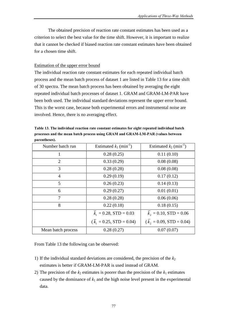
77

The obtained precision of reaction rate constant estimates has been used as a

criterion to select the best value for the time shift. However, it is important to realize

that it cannot be checked if biased reaction rate constant estimates have been obtained

for a chosen time shift.

Estimation of the upper error bound

The individual reaction rate constant estimates for each repeated individual batch

process and the mean batch process of dataset 1 are listed in Table 13 for a time shift

of 30 spectra. The mean batch process has been obtained by averaging the eight

repeated individual batch processes of dataset 1. GRAM and GRAM-LM-PAR have

been both used. The individual standard deviations represent the upper error bound.

This is the worst case, because both experimental errors and instrumental noise are

involved. Hence, there is no averaging effect.

��#�� '�� $��&��'��#��

�� $��#�� &�-��-��.��/��('��#��%��

��+�

Number batch run Estimated �1 (min-1) Estimated �2 (min-1)

1 0.28 (0.25) 0.11 (0.10)

2 0.33 (0.29) 0.08 (0.08)

3 0.28 (0.28) 0.08 (0.08)

4 0.29 (0.19) 0.17 (0.12)

5 0.26 (0.23) 0.14 (0.13)

6 0.29 (0.27) 0.01 (0.01)

7 0.28 (0.28) 0.06 (0.06)

8 0.22 (0.18) 0.18 (0.15)

�1 = 0.28, STD = 0.03

( �1 = 0.25, STD = 0.04)

2� = 0.10, STD = 0.06

( 2� = 0.09, STD = 0.04)

Mean batch process 0.28 (0.27) 0.07 (0.07)

From Table 13 the following can be observed:

1) If the individual standard deviations are considered, the precision of the �2

estimates is better if GRAM-LM-PAR is used instead of GRAM.

2) The precision of the �2 estimates is poorer than the precision of the �1 estimates

caused by the dominance of �1 and the high noise level present in the experimental

data.

��

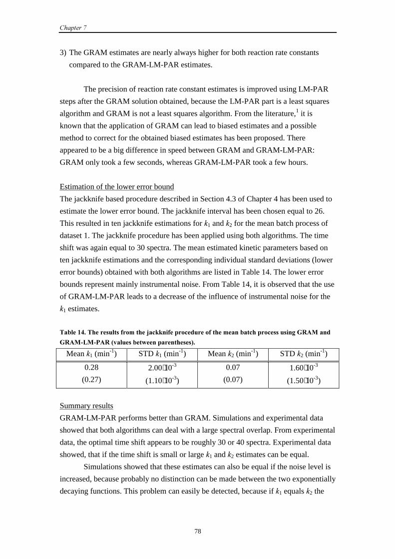
78

3) The GRAM estimates are nearly always higher for both reaction rate constants

compared to the GRAM-LM-PAR estimates.

The precision of reaction rate constant estimates is improved using LM-PAR

steps after the GRAM solution obtained, because the LM-PAR part is a least squares

algorithm and GRAM is not a least squares algorithm. From the literature,1 it is

known that the application of GRAM can lead to biased estimates and a possible

method to correct for the obtained biased estimates has been proposed. There

appeared to be a big difference in speed between GRAM and GRAM-LM-PAR:

GRAM only took a few seconds, whereas GRAM-LM-PAR took a few hours.

Estimation of the lower error bound

The jackknife based procedure described in Section 4.3 of Chapter 4 has been used to

estimate the lower error bound. The jackknife interval has been chosen equal to 26.

This resulted in ten jackknife estimations for �1 and �2 for the mean batch process of

dataset 1. The jackknife procedure has been applied using both algorithms. The time

shift was again equal to 30 spectra. The mean estimated kinetic parameters based on

ten jackknife estimations and the corresponding individual standard deviations (lower

error bounds) obtained with both algorithms are listed in Table 14. The lower error

bounds represent mainly instrumental noise. From Table 14, it is observed that the use

of GRAM-LM-PAR leads to a decrease of the influence of instrumental noise for the

�1 estimates.

��#��3��$��4� 55�� $��#�� &�-��

-��.��/��('��#��%��+�

Mean �1 (min-1) STD �1 (min-1) Mean �2 (min-1) STD �2 (min-1)

0.28

(0.27)

2.00⋅10-3

(1.10⋅10-3)

0.07

(0.07)

1.60⋅10-3

(1.50⋅10-3)

Summary results

GRAM-LM-PAR performs better than GRAM. Simulations and experimental data

showed that both algorithms can deal with a large spectral overlap. From experimental

data, the optimal time shift appears to be roughly 30 or 40 spectra. Experimental data

showed, that if the time shift is small or large �1 and �2 estimates can be equal.

Simulations showed that these estimates can also be equal if the noise level is

increased, because probably no distinction can be made between the two exponentially

decaying functions. This problem can easily be detected, because if �1 equals �2 the

�� !�"�#��

79

first two columns of the �-matrix (loading matrix obtained by solving a GEP) are

identical. If the upper error bound is considered and the performance of

GRAM-LM-PAR is compared to the performance of GRAM, the precision of the �2

estimates is the best if GRAM-LM-PAR is used. The GRAM estimates are always

higher than the GRAM-LM-PAR estimates. For the lower error bound the precision of

the �1 estimates is approximately a factor two better using GRAM-LM-PAR instead of

GRAM. Despite the fact that the precision of reaction rate constant estimates is poorer

if GRAM is used instead of GRAM-LM-PAR, GRAM is very powerful if rapid

estimates of reaction rate constants are necessary.

��$��

In this Section, GRAM has been used in order to estimate reaction rate constants from

on-line SW-NIR measurements (dataset 1) of a reacting system. The interpretation is

very easy. The third factor matrix of the three-way array, �, gives the reaction rate

constants. GRAM-LM-PAR can be used if precise estimates of reaction rate constants

are desirable. GRAM can be used to obtain rough estimations of reaction rate

constants very fast. Simulations showed that both algorithms can deal with a strong

spectral overlap. If the noise level is increased the reaction rate constants estimates

can become equal for a simulated dataset. From the simulations it can be concluded,

that GRAM-LM-PAR always leads to more precise estimates of reaction rate

constants compared to GRAM, because the LM-PAR part of GRAM-LM-PAR is a

least squares algorithm.

The results obtained from dataset 1 showed a small difference between GRAM

and GRAM-LM-PAR, but GRAM-LM-PAR always leads to more precise estimates

for the reaction rate constants compared to GRAM. The optimal time shift appeared to

be roughly 30 or 40 spectra in this case. If the time shift parameter is large or small the

reaction rate constant estimates can become equal and a poor precision of reaction rate

constant estimates is obtained. Probably, it is very hard to distinguish between

exponentially decaying functions for these choices of the time shift parameter. Upper

and lower error bounds have been estimated also for quality assessment.

GRAM is a very powerful method for estimating reaction rate constants very

fast. The speed of the algorithm is known in advance, because of its non-iterative

nature. GRAM can be used if rough estimates of kinetic parameters are desirable, for

instance if (batch) processes are monitored. GRAM-LM-PAR is in this case not very

convenient to use because of the time consuming iterations. In case of

GRAM-LM-PAR the speed of the algorithm is not known in advance. If the batch

time is elapsed GRAM-LM-PAR can be used to estimate kinetic parameters precisely.

Since many measurements are based on exponential functions, GRAM and

��

80

GRAM-LM-PAR can have many applications in chemistry.

� �67�7��

��

In this Section, GRAM and GRAM-LM-PAR are applied in order to estimate reaction

rate constants from the UV-Vis measurements of dataset 2, described in Section 5.3 of

Chapter 5. The choice of the time shift parameter has been investigated. The pure

spectra of the reacting absorbing species are estimated very easily, without

complicated procedures, and compared to their measured pure spectra. If species are

unknown, spectrum library search methods can be used to identify the estimated pure

spectra of these unknown species. Quality assessment of the estimated reaction rate

constants has been performed using a jackknife based method, described in

Section 4.3 of Chapter 4.

��

EFFECT OF THE TIME SHIFT ON REACTION RATE CONSTANT ESTIMATES

In order to investigate the effect of different time shifts, the kinetic parameters have

been estimated for the ten repeated individual batch processes of dataset 2 using

GRAM for different time shifts. The results are listed in Table 15. The values of the

column with constants added to " were equal to 100000. These values will dominate

compared to the absorbances differences in time of the UV-Vis spectra (see Figure 14,

Section 5.3.3, Chapter 5). From Table 15 the following can be observed:

1) A small time shift results in a poor precision for both �1 and �2 estimates.

2) A large time shift results in a poor precision for the �1 estimates and a good

precision for the �2 estimates.

3) A time shift of 30 spectra is a compromise, because this gives the best precision for

�1 estimates and a compromise in precision for the �2 estimates. For this reason a

time shift of 30 spectra is used for dataset 2 in the remainder of this Chapter.

An important remark is the computation time of reaction rate constants using GRAM

or GRAM-LM-PAR. In this case GRAM takes only a few seconds, but

GRAM-LM-PAR takes a few hours to perform the necessary iterations, approximately

4000-5000. Hence, GRAM is very fast. The aspects mentioned concerning the

computation time were also observed for the SW-NIR dataset investigated in

Section 7.2 of this Chapter.

�� !�"�#��

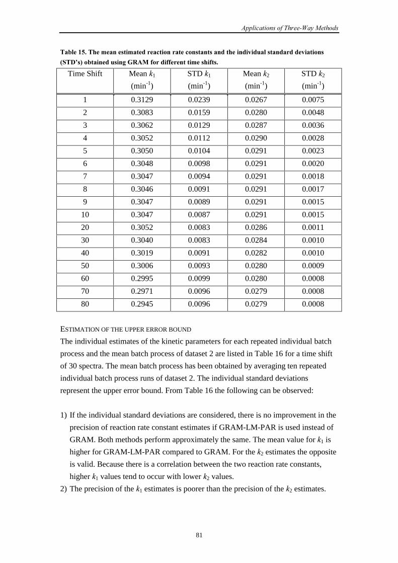
81

��#��8��$��$�� '��'��

(��)*�+��#��&�-��$��

Time Shift Mean �1

(min-1)

STD �1

(min-1)

Mean �2

(min-1)

STD �2

(min-1)

1 0.3129 0.0239 0.0267 0.0075

2 0.3083 0.0159 0.0280 0.0048

3 0.3062 0.0129 0.0287 0.0036

4 0.3052 0.0112 0.0290 0.0028

5 0.3050 0.0104 0.0291 0.0023

6 0.3048 0.0098 0.0291 0.0020

7 0.3047 0.0094 0.0291 0.0018

8 0.3046 0.0091 0.0291 0.0017

9 0.3047 0.0089 0.0291 0.0015

10 0.3047 0.0087 0.0291 0.0015

20 0.3052 0.0083 0.0286 0.0011

30 0.3040 0.0083 0.0284 0.0010

40 0.3019 0.0091 0.0282 0.0010

50 0.3006 0.0093 0.0280 0.0009

60 0.2995 0.0099 0.0280 0.0008

70 0.2971 0.0096 0.0279 0.0008

80 0.2945 0.0096 0.0279 0.0008

ESTIMATION OF THE UPPER ERROR BOUND

The individual estimates of the kinetic parameters for each repeated individual batch

process and the mean batch process of dataset 2 are listed in Table 16 for a time shift

of 30 spectra. The mean batch process has been obtained by averaging ten repeated

individual batch process runs of dataset 2. The individual standard deviations

represent the upper error bound. From Table 16 the following can be observed:

1) If the individual standard deviations are considered, there is no improvement in the

precision of reaction rate constant estimates if GRAM-LM-PAR is used instead of

GRAM. Both methods perform approximately the same. The mean value for �1 is

higher for GRAM-LM-PAR compared to GRAM. For the �2 estimates the opposite

is valid. Because there is a correlation between the two reaction rate constants,

higher �1 values tend to occur with lower �2 values.

2) The precision of the �1 estimates is poorer than the precision of the �2 estimates.

��

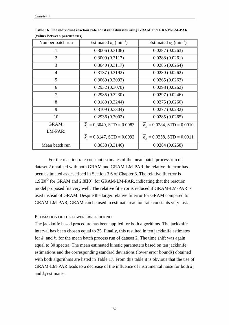
82

��#��!��'�� $��&�-��-��.��/�

('��#��%��+�

Number batch run Estimated �1 (min-1) Estimated �2 (min-1)

1 0.3006 (0.3106) 0.0287 (0.0263)

2 0.3009 (0.3117) 0.0288 (0.0261)

3 0.3040 (0.3117) 0.0285 (0.0264)

4 0.3137 (0.3192) 0.0280 (0.0262)

5 0.3069 (0.3093) 0.0265 (0.0263)

6 0.2932 (0.3070) 0.0298 (0.0262)

7 0.2985 (0.3230) 0.0297 (0.0246)

8 0.3180 (0.3244) 0.0275 (0.0260)

9 0.3109 (0.3304) 0.0277 (0.0232)

10 0.2936 (0.3002) 0.0285 (0.0265)

GRAM:

LM-PAR:�1 = 0.3040, STD = 0.0083

�1 = 0.3147, STD = 0.0092

2� = 0.0284, STD = 0.0010

2� = 0.0258, STD = 0.0011

Mean batch run 0.3038 (0.3146) 0.0284 (0.0258)

For the reaction rate constant estimates of the mean batch process run of

dataset 2 obtained with both GRAM and GRAM-LM-PAR the relative fit error has

been estimated as described in Section 3.6 of Chapter 3. The relative fit error is

1.9⋅10-3 for GRAM and 2.8⋅10-4 for GRAM-LM-PAR, indicating that the reaction

model proposed fits very well. The relative fit error is reduced if GRAM-LM-PAR is

used instead of GRAM. Despite the larger relative fit error for GRAM compared to

GRAM-LM-PAR, GRAM can be used to estimate reaction rate constants very fast.

ESTIMATION OF THE LOWER ERROR BOUND

The jackknife based procedure has been applied for both algorithms. The jackknife

interval has been chosen equal to 25. Finally, this resulted in ten jackknife estimates

for �1 and �2 for the mean batch process run of dataset 2. The time shift was again

equal to 30 spectra. The mean estimated kinetic parameters based on ten jackknife

estimations and the corresponding standard deviations (lower error bounds) obtained

with both algorithms are listed in Table 17. From this table it is obvious that the use of

GRAM-LM-PAR leads to a decrease of the influence of instrumental noise for both �1

and �2 estimates.

�� !�"�#��

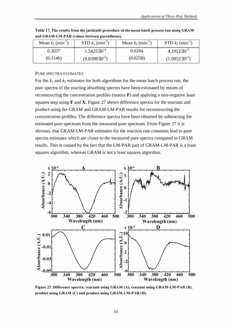
83

��#��$��4� 55�� $��#�� &�-��

��-��.��/��('��#��%��+�

Mean �1 (min-1) STD �1 (min-1) Mean �2 (min-1) STD �2 (min-1)

0.3037

(0.3146)

1.5425⋅10-4

(9.8398⋅10-5)

0.0284

(0.0258)

4.1912⋅10-5

(1.0852⋅10-5)

PURE SPECTRA ESTIMATES

For the �1 and �2 estimates for both algorithms for the mean batch process run, the

pure spectra of the reacting absorbing species have been estimated by means of

reconstructing the concentration profiles (matrix 9) and applying a non-negative least

squares step using 9 and ". Figure 27 shows difference spectra for the reactant and

product using the GRAM and GRAM-LM-PAR results for reconstructing the

concentration profiles. The difference spectra have been obtained by subtracting the

estimated pure spectrum from the measured pure spectrum. From Figure 27 it is

obvious, that GRAM-LM-PAR estimates for the reaction rate constants lead to pure

spectra estimates which are closer to the measured pure spectra compared to GRAM

results. This is caused by the fact that the LM-PAR part of GRAM-LM-PAR is a least

squares algorithm, whereas GRAM is not a least squares algorithm.

8,, ,, 3, :, 3�, 3!, 8,,��

��

,

�

0��,��

8,,

��'��&��(�$+

��'��&��(�$+

#��#�

� ��(

�6�+

,, 3, :, 3�, 3!,�!

�3

��

,

�0��,��

��'��&��(�$+

#��#�

� ��(

�6�+

,, 3, :, 3�, 3!,�,�,8

�,�,

�,�,�

,�,�

#��#�

� ��(

�6�+

��'��&��(�$+

#��#�

� ��(

�6�+

,, 3, :, 3�, 3!, 8,,�!

��

�

!

�,0��,��

�

;

)

9�&��)�� <�� &�-��(+=�� &�-��.��/��(;+=

�� &�-��(�+�� &�-��.��/��()+�

��

84

SUMMARY RESULTS

A time shift of 30 spectra appeared to give the best precision for the �1 estimates and a

compromise in precision for the �2 estimates if GRAM was used. For all the different

batch process runs the reaction rate constants have been obtained both with GRAM

and GRAM-LM-PAR for this time shift of 30 spectra. The obtained precision for the

reaction rate constant estimates showed that there is hardly a difference in

performance between GRAM and GRAM-LM-PAR. This is probably caused by the

fact that the signal to noise ratio of the dataset is excellent and the absorbance

differences in time are very large. For the mean batch process run the reaction rate

constants have been estimated using both algorithms. The relative fit errors are

1.9⋅10-3 and 2.8⋅10-4 for GRAM and GRAM-LM-PAR, respectively. These values

indicate that the kinetic model proposed fitted the best using GRAM-LM-PAR.

However, the fit error value for GRAM is still acceptable. The jackknife procedure

showed that the influence of the instrumental noise on the precision of both reaction

rate constant estimates is smaller using GRAM-LM-PAR compared to GRAM.

Finally, the pure spectra have been estimated for the GRAM-LM-PAR and

GRAM results. The pure spectra of reactant and product showed a very good

agreement with the measured pure spectra. The difference between the estimated pure

spectra and the measured pure spectra is smaller for reaction rate constants which

have been obtained by GRAM-LM-PAR compared to the GRAM results.

��

In this Section, it is shown that GRAM can be used as a very fast non-iterative

algorithm in order to estimate reaction rate constants from the UV-Vis spectra of

dataset 2. The precision of the reaction rate constant estimates is comparable to the

precision obtained with GRAM-LM-PAR. However, GRAM gives a larger fit error.

GRAM-LM-PAR can be used in situations where an accurate estimate of reaction rate

constants is desirable and there is enough time available to perform the tedious

iterations (approximately 4000-5000) which characterizes the GRAM-LM-PAR

algorithm. A time shift of 30 spectra appeared to be optimal for this application. This

has to be established in practice again for other kinetic model systems.

If the pure spectra estimates of the reacting absorbing species involved in the

reaction model are compared with the measured pure spectra the difference is very

small. GRAM-LM-PAR gives better pure spectra estimates compared to GRAM.

�3�-��

�� !�"�#��

85

From the results described in this Chapter obtained with dataset 1 and dataset 2, some

general conclusions can be formulated:

1) For noisy datasets (dataset 1 in this case) GRAM-LM-PAR leads to a better

precision of reaction rate constant estimates compared to GRAM, because the

LM-PAR part is a least squares algorithm.

2) For datasets with an excellent signal to noise ratio and large absorbance differences

in time (dataset 2 in this case) GRAM-LM-PAR and GRAM perform the same

with respect to the precision of reaction rate constant estimates. Hence, if the noise

level of the data is low a least squares algorithm will hardly improve the precision

of parameter estimates. However, a lower fit error is obtained for

GRAM-LM-PAR.

�8�� 1. Faber K, Lorber A, Kowalski BR. ‘Generalized rank annihilation method: Standard errors in the

estimated eigenvalues of the instrumental errors are heteroscedastic and correlated’.

�� , 1997; ��: 95-110.

��

86

87

��

��

��

��

In Chapter 6 and 7, applications of two-way and three-way methods to different

datasets have been discussed. In this Chapter,i the performance of classical curve

resolution (CCR) with constraint RP implemented (see Section 2.7, Chapter 2),

weighted curve resolution (WCR), the generalized rank annihilation method (GRAM),

the generalized rank annihilation-Levenberg-Marquardt-parallel factor analysis

(GRAM-LM-PAR) method, the trilinear decomposition method (TLD) and the

trilinear decomposition method-Levenberg-Marquardt-parallel factor analysis

(TLD-LM-PAR) method are compared. This is the only Chapter of the thesis where

results obtained with TLD and TLD-LM-PAR are reported. The theory of TLD and

TLD-LM-PAR has been described in Chapter 3. Because of the comparison of

two-way and three-way methods, some results described already in Chapter 6 and 7

are repeated in this Chapter, which is unavoidable. The starting values of the reaction

rate constants used for the two-way methods have been reported in Section 5.2.4 and

Section 5.3.5 of Chapter 5. If other sets of starting values were used, similar results

were obtained.

�� !�!� ��

��

In this Section, the precision and speed of CCR using �� spectral information

(constraint RP), WCR, GRAM, GRAM-LM-PAR, TLD and TLD-LM-PAR are

compared using dataset 1 and dataset 2. These datasets have been described in

i This Chapter is based on the following paper:

� Bijlsma S, Smilde AK. ‘Estimating reaction rate constants from a two-step reaction: comparison

between two-way and three-way methods’. �� , accepted.

��

88

Section 5.2 and Section 5.3 of Chapter 5. The theory of the algorithms has been

described in Chapter 2 (two-way methods) and Chapter 3 (three-way methods).

Important properties of CCR, WCR, GRAM, GRAM-LM-PAR, TLD and

TLD-LM-PAR are summarized in Table 18. All methods are least squares methods

except GRAM and TLD. Dataset 1 has a moderate signal to noise ratio and dataset 2

has a high signal to noise ratio. Hence, both datasets represent extremes of what can

be expected in chemical practice. In case of CCR using �� spectral information,

the pure spectra of reactant and product have been explicitly implemented in the

algorithm resulting in constraint RP as described in Section 2.7 of Chapter 2. Quality

assessment has been performed using a jackknife based method presented in

Section 4.3 of Chapter 4.

��"#�� $��%��%�&�'�%�&�'��(��)'�%��(*��

�(*�(��)'�� $� ��++�� #� �� ,$� �-%�+��

�� ,��-�� ##�� , #�-�

Algorithm A priori

information

Time

shift

Number

of slabs

Iterative Speed On-line

CCR yes no 1 yes + no

WCR no no 1 yes + no

GRAM no yes 2 no ++ yes

GRAM-LM-PAR no yes 2 yes - no

TLD no yes ≥ 3 no ++ yes

TLD-LM-PAR no yes ≥ 3 yes - no

��

REACTION RATE CONSTANT ESTIMATES FROM INDIVIDUAL BATCH PROCESSES

Dataset 1

For eight individual batch process runs of dataset 1, the reaction rate constants have

been estimated using WCR, GRAM, GRAM-LM-PAR, TLD (three and four slabs)

and TLD-LM-PAR (three slabs). The results are listed in Table 19. The individual

standard deviations represent the upper error bounds. The correlation coefficients, ,

between the reaction rate constant estimates have been calculated and are also listed in

Table 19. The absolute value for gives an indication about the quality of the

algorithm used. A small absolute value of indicates that the algorithm can

distinguish between �1 and �2 during the optimization procedure very easily. For

GRAM and GRAM-LM-PAR the time shift was equal to 30 spectra. From Chapter 7

it appeared that this time shift led to the best precision of the �1 and �2 estimates. For

TLD and TLD-LM-PAR the step size was equal to 20 spectra. It appeared that these

��

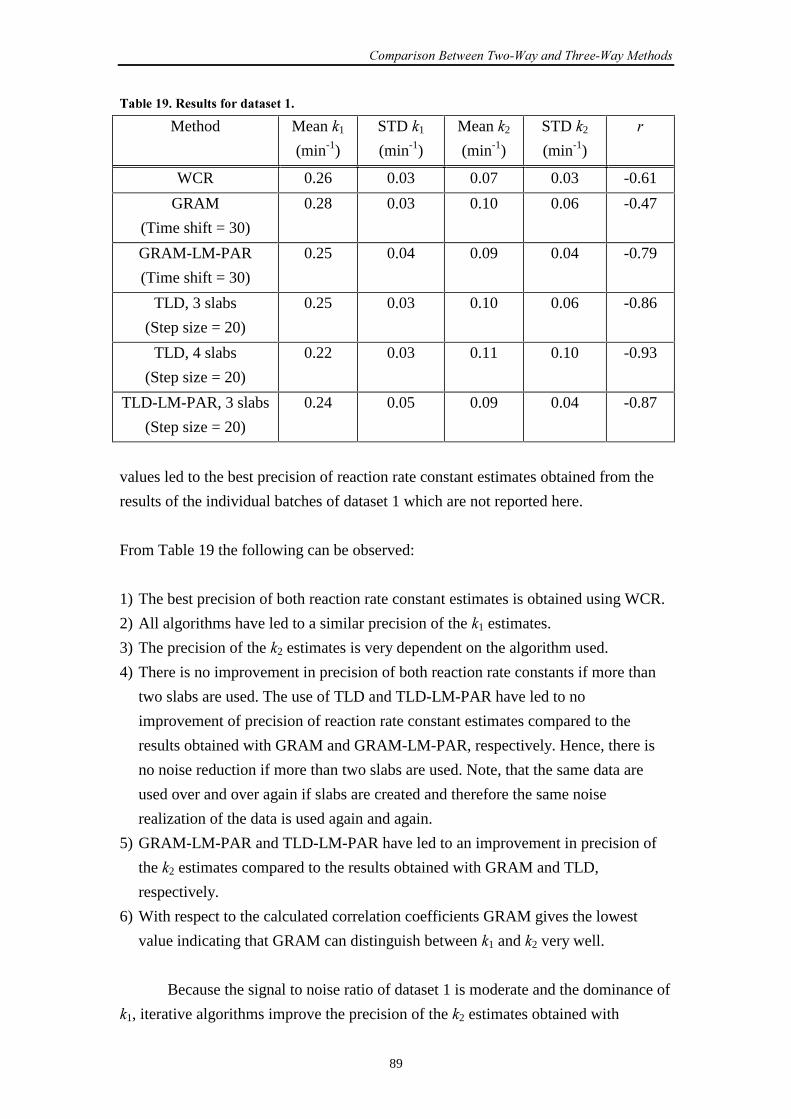
89

��"#��.�� #� �$��

Method Mean �1

(min-1)

STD �1

(min-1)

Mean �2

(min-1)

STD �2

(min-1)

WCR 0.26 0.03 0.07 0.03 -0.61

GRAM

(Time shift = 30)

0.28 0.03 0.10 0.06 -0.47

GRAM-LM-PAR

(Time shift = 30)

0.25 0.04 0.09 0.04 -0.79

TLD, 3 slabs

(Step size = 20)

0.25 0.03 0.10 0.06 -0.86

TLD, 4 slabs

(Step size = 20)

0.22 0.03 0.11 0.10 -0.93

TLD-LM-PAR, 3 slabs

(Step size = 20)

0.24 0.05 0.09 0.04 -0.87

values led to the best precision of reaction rate constant estimates obtained from the

results of the individual batches of dataset 1 which are not reported here.


1) The best precision of both reaction rate constant estimates is obtained using WCR.

2) All algorithms have led to a similar precision of the �1 estimates.

3) The precision of the �2 estimates is very dependent on the algorithm used.

4) There is no improvement in precision of both reaction rate constants if more than

two slabs are used. The use of TLD and TLD-LM-PAR have led to no

improvement of precision of reaction rate constant estimates compared to the

results obtained with GRAM and GRAM-LM-PAR, respectively. Hence, there is

no noise reduction if more than two slabs are used. Note, that the same data are

used over and over again if slabs are created and therefore the same noise

realization of the data is used again and again.

5) GRAM-LM-PAR and TLD-LM-PAR have led to an improvement in precision of

the �2 estimates compared to the results obtained with GRAM and TLD,

respectively.

6) With respect to the calculated correlation coefficients GRAM gives the lowest

value indicating that GRAM can distinguish between �1 and �2 very well.

Because the signal to noise ratio of dataset 1 is moderate and the dominance of

�1, iterative algorithms improve the precision of the �2 estimates obtained with

��

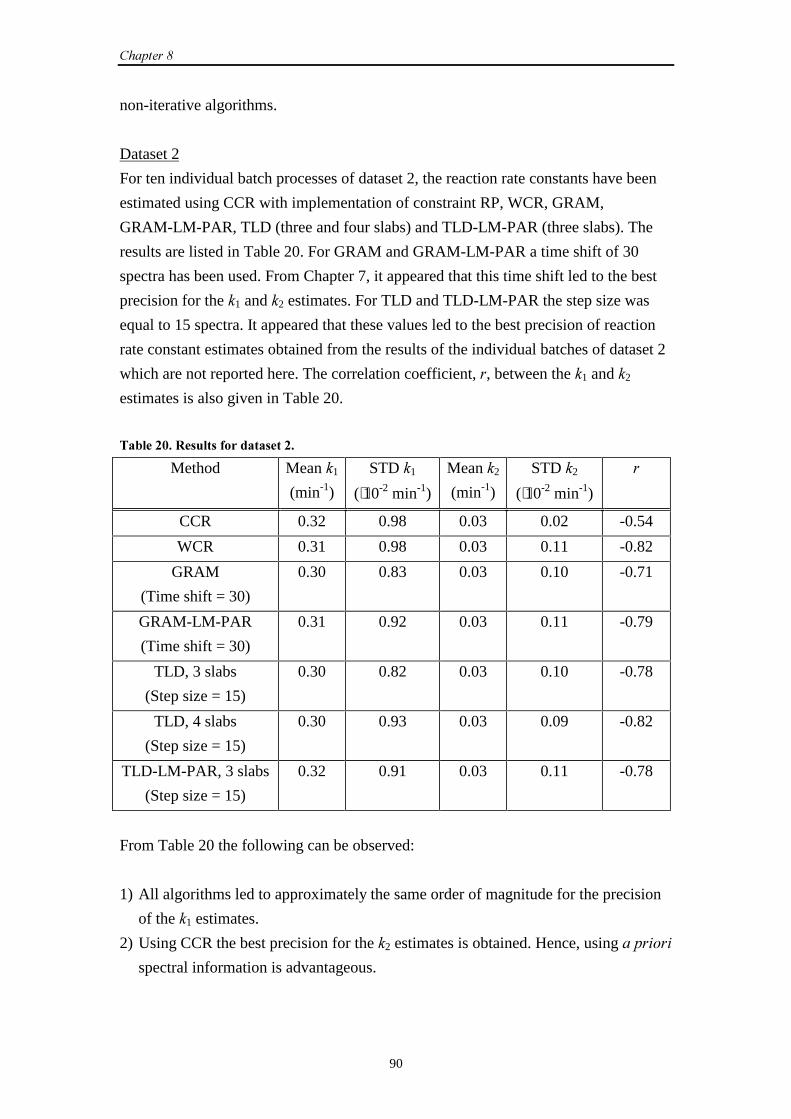
90

non-iterative algorithms.

Dataset 2

For ten individual batch processes of dataset 2, the reaction rate constants have been

estimated using CCR with implementation of constraint RP, WCR, GRAM,

GRAM-LM-PAR, TLD (three and four slabs) and TLD-LM-PAR (three slabs). The

results are listed in Table 20. For GRAM and GRAM-LM-PAR a time shift of 30

spectra has been used. From Chapter 7, it appeared that this time shift led to the best

precision for the �1 and �2 estimates. For TLD and TLD-LM-PAR the step size was

equal to 15 spectra. It appeared that these values led to the best precision of reaction

rate constant estimates obtained from the results of the individual batches of dataset 2

which are not reported here. The correlation coefficient, , between the �1 and �2

estimates is also given in Table 20.

��"#��/�� #� �$��

Method Mean �1

(min-1)

STD �1

(⋅10-2 min-1)

Mean �2

(min-1)

STD �2

(⋅10-2 min-1)

CCR 0.32 0.98 0.03 0.02 -0.54

WCR 0.31 0.98 0.03 0.11 -0.82

GRAM

(Time shift = 30)

0.30 0.83 0.03 0.10 -0.71

GRAM-LM-PAR

(Time shift = 30)

0.31 0.92 0.03 0.11 -0.79

TLD, 3 slabs

(Step size = 15)

0.30 0.82 0.03 0.10 -0.78

TLD, 4 slabs

(Step size = 15)

0.30 0.93 0.03 0.09 -0.82

TLD-LM-PAR, 3 slabs

(Step size = 15)

0.32 0.91 0.03 0.11 -0.78


1) All algorithms led to approximately the same order of magnitude for the precision

of the �1 estimates.

2) Using CCR the best precision for the �2 estimates is obtained. Hence, using ��

spectral information is advantageous.

��

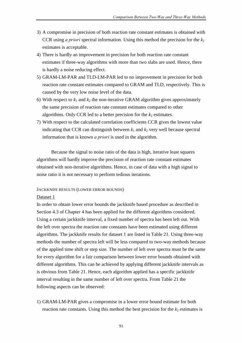
91

3) A compromise in precision of both reaction rate constant estimates is obtained with

CCR using �� spectral information. Using this method the precision for the �1

estimates is acceptable.

4) There is hardly an improvement in precision for both reaction rate constant

estimates if three-way algorithms with more than two slabs are used. Hence, there

is hardly a noise reducing effect.

5) GRAM-LM-PAR and TLD-LM-PAR led to no improvement in precision for both

reaction rate constant estimates compared to GRAM and TLD, respectively. This is

caused by the very low noise level of the data.

6) With respect to �1 and �2 the non-iterative GRAM algorithm gives approximately

the same precision of reaction rate constant estimates compared to other

algorithms. Only CCR led to a better precision for the �2 estimates.

7) With respect to the calculated correlation coefficients CCR gives the lowest value

indicating that CCR can distinguish between �1 and �2 very well because spectral

information that is known �� is used in the algorithm.

Because the signal to noise ratio of the data is high, iterative least squares

algorithms will hardly improve the precision of reaction rate constant estimates

obtained with non-iterative algorithms. Hence, in case of data with a high signal to

noise ratio it is not necessary to perform tedious iterations.

JACKKNIFE RESULTS (LOWER ERROR BOUNDS)

Dataset 1

In order to obtain lower error bounds the jackknife based procedure as described in

Section 4.3 of Chapter 4 has been applied for the different algorithms considered.

Using a certain jackknife interval, a fixed number of spectra has been left out. With

the left over spectra the reaction rate constants have been estimated using different

algorithms. The jackknife results for dataset 1 are listed in Table 21. Using three-way

methods the number of spectra left will be less compared to two-way methods because

of the applied time shift or step size. The number of left over spectra must be the same

for every algorithm for a fair comparison between lower error bounds obtained with

different algorithms. This can be achieved by applying different jackknife intervals as

is obvious from Table 21. Hence, each algorithm applied has a specific jackknife

interval resulting in the same number of left over spectra. From Table 21 the

following aspects can be observed:

1) GRAM-LM-PAR gives a compromise in a lower error bound estimate for both

reaction rate constants. Using this method the best precision for the �2 estimates is

��

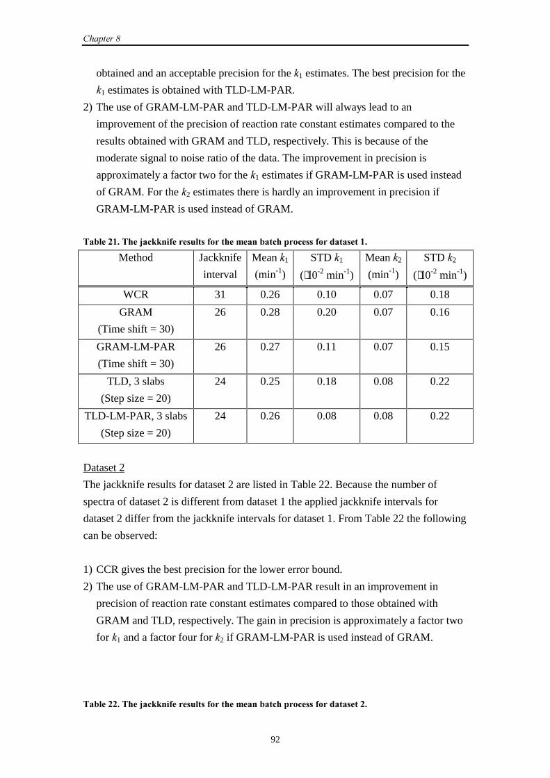
92

obtained and an acceptable precision for the �1 estimates. The best precision for the

�1 estimates is obtained with TLD-LM-PAR.

2) The use of GRAM-LM-PAR and TLD-LM-PAR will always lead to an

improvement of the precision of reaction rate constant estimates compared to the

results obtained with GRAM and TLD, respectively. This is because of the

moderate signal to noise ratio of the data. The improvement in precision is

approximately a factor two for the �1 estimates if GRAM-LM-PAR is used instead

of GRAM. For the �2 estimates there is hardly an improvement in precision if

GRAM-LM-PAR is used instead of GRAM.

��"#��0��11��$�� #� �$��"�� $��

Method Jackknife

interval

Mean �1

(min-1)

STD �1

(⋅10-2 min-1)

Mean �2

(min-1)

STD �2

(⋅10-2 min-1)

WCR 31 0.26 0.10 0.07 0.18

GRAM

(Time shift = 30)

26 0.28 0.20 0.07 0.16

GRAM-LM-PAR

(Time shift = 30)

26 0.27 0.11 0.07 0.15

TLD, 3 slabs

(Step size = 20)

24 0.25 0.18 0.08 0.22

TLD-LM-PAR, 3 slabs

(Step size = 20)

24 0.26 0.08 0.08 0.22

Dataset 2

The jackknife results for dataset 2 are listed in Table 22. Because the number of

spectra of dataset 2 is different from dataset 1 the applied jackknife intervals for

dataset 2 differ from the jackknife intervals for dataset 1. From Table 22 the following

can be observed:

1) CCR gives the best precision for the lower error bound.

2) The use of GRAM-LM-PAR and TLD-LM-PAR result in an improvement in

precision of reaction rate constant estimates compared to those obtained with

GRAM and TLD, respectively. The gain in precision is approximately a factor two

for �1 and a factor four for �2 if GRAM-LM-PAR is used instead of GRAM.

��"#��0��11��$�� #� �$��"�� $��

��

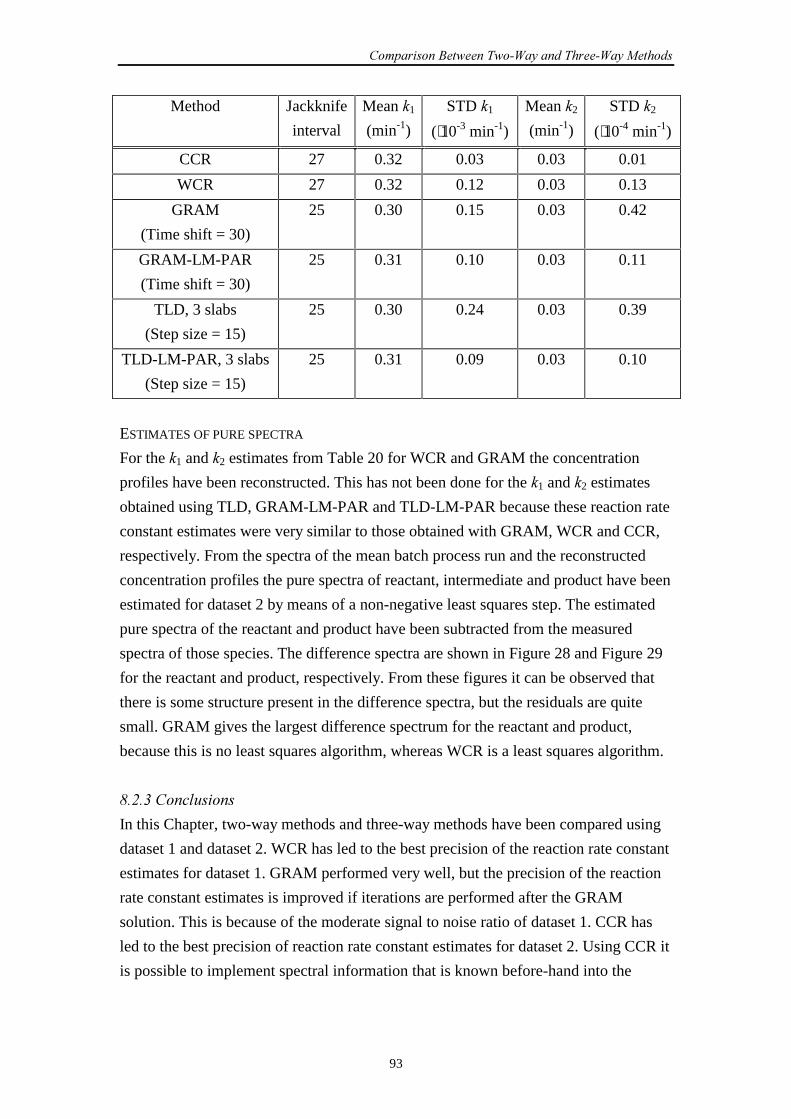
93

Method Jackknife

interval

Mean �1

(min-1)

STD �1

(⋅10-3 min-1)

Mean �2

(min-1)

STD �2

(⋅10-4 min-1)

CCR 27 0.32 0.03 0.03 0.01

WCR 27 0.32 0.12 0.03 0.13

GRAM

(Time shift = 30)

25 0.30 0.15 0.03 0.42

GRAM-LM-PAR

(Time shift = 30)

25 0.31 0.10 0.03 0.11

TLD, 3 slabs

(Step size = 15)

25 0.30 0.24 0.03 0.39

TLD-LM-PAR, 3 slabs

(Step size = 15)

25 0.31 0.09 0.03 0.10

ESTIMATES OF PURE SPECTRA

For the �1 and �2 estimates from Table 20 for WCR and GRAM the concentration

profiles have been reconstructed. This has not been done for the �1 and �2 estimates

obtained using TLD, GRAM-LM-PAR and TLD-LM-PAR because these reaction rate

constant estimates were very similar to those obtained with GRAM, WCR and CCR,

respectively. From the spectra of the mean batch process run and the reconstructed

concentration profiles the pure spectra of reactant, intermediate and product have been

estimated for dataset 2 by means of a non-negative least squares step. The estimated

pure spectra of the reactant and product have been subtracted from the measured

spectra of those species. The difference spectra are shown in Figure 28 and Figure 29

for the reactant and product, respectively. From these figures it can be observed that

there is some structure present in the difference spectra, but the residuals are quite

small. GRAM gives the largest difference spectrum for the reactant and product,

because this is no least squares algorithm, whereas WCR is a least squares algorithm.

��!��

In this Chapter, two-way methods and three-way methods have been compared using

dataset 1 and dataset 2. WCR has led to the best precision of the reaction rate constant

estimates for dataset 1. GRAM performed very well, but the precision of the reaction

rate constant estimates is improved if iterations are performed after the GRAM

solution. This is because of the moderate signal to noise ratio of dataset 1. CCR has

led to the best precision of reaction rate constant estimates for dataset 2. Using CCR it

is possible to implement spectral information that is known before-hand into the

��

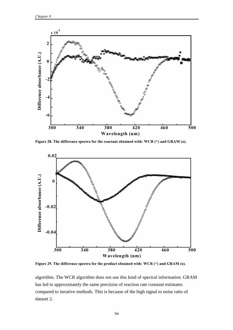
94

��2�#��3��,��-

*�$$��" �"��,'� �-

4// 45/ 4/ 5�/ 56/ 7//

�6

�5

��

/

�

8��/��

9�3��$$�� $��"��:��,;-��&�'��,-�

*�$$��" �"��,'� �-

��2�#��3��,��-4// 45/ 4/ 5�/ 56/ 7//

�/�/5

�/�/�

/

/�/�

9�3��.��$$�� $��"��:��,;-��&�'��,-�

algorithm. The WCR algorithm does not use this kind of spectral information. GRAM

has led to approximately the same precision of reaction rate constant estimates

compared to iterative methods. This is because of the high signal to noise ratio of

dataset 2.

��

95

In general, two-way methods will lead to a better precision of reaction rate

constant estimates compared to three-way methods. For every specific dataset a

certain two-way algorithm will perform the best. The two-way methods CCR and

WCR are both of medium speed. Because of the iterative nature of both WCR and

CCR the exact speed of the algorithm needed to reach the optimal set of parameters is

not known beforehand. This is dependent on the choice of the set of starting values.

This makes CCR and WCR less suitable for on-line estimating reaction rate constants.

In practice it is very often not necessary to know the values of reaction rate constants

very precisely. Hence, it is not always necessary to use iterative algorithms. GRAM

can be very convenient to use in that case, because the speed of this algorithm is

known in advance. This makes GRAM extraordinarily suitable for on-line monitoring

reaction rate constants. Both datasets used showed good results using GRAM and

hence this method seems to be the best choice for on-line (pseudo) first order kinetic

problems. For noisy datasets more reliable estimates of reaction rate constants can be

obtained off-line using iterative algorithms.

��

96

97

��

��

��

��

In this Chapter,i the impact of constraints implemented in classical curve resolution

(CCR) on the precision of reaction rate constant estimates is investigated using

experimental data. Simulated data are used to study the impact of constraints in CCR

on the accuracy of reaction rate constant estimates. Simulated data are also used to

check if biased estimates are obtained using CCR with and without constraints

implemented. The equations used to calculate the precision, the bias, the accuracy and

the relative errors of reaction rate constant estimates have been presented in

Section 4.2 of Chapter 4. Constraint R, constraint RP and constraint NNLS, which can

be implemented in CCR, have already been discussed in Section 2.7 of Chapter 2. The

starting values of the reaction rate constants used for the two-way methods have been

reported in Section 5.3.5 of Chapter 5. If other sets of starting values were used,

similar results were obtained.

��

��

The goal of this Chapter is to determine the impact of the use of constraints in CCR

on the accuracy of the reaction rate constant estimates, to establish whether it is an

advantage to use constraints and to define guidelines for the use of constraints. This

thesis reports a systematic study on this topic.

From dataset 3, described in Section 5.3 of Chapter 5, reaction rate constants

and pure spectra of individual reacting absorbing species have been estimated

simultaneously with and without constraints implemented in CCR. For the

experimental data only the precision of the reaction rate constant estimates could be

i This Chapter is based on the following paper:

� Bijlsma S, Boelens HFM, Hoefsloot HCJ, Smilde AK. ‘Constrained least squares methods for

estimating reaction rate constants from spectroscopic data’. submitted.

��

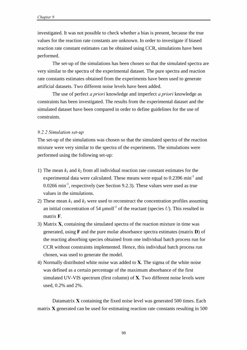
98

investigated. It was not possible to check whether a bias is present, because the true

values for the reaction rate constants are unknown. In order to investigate if biased

reaction rate constant estimates can be obtained using CCR, simulations have been

performed.

The set-up of the simulations has been chosen so that the simulated spectra are

very similar to the spectra of the experimental dataset. The pure spectra and reaction

rate constants estimates obtained from the experiments have been used to generate

artificial datasets. Two different noise levels have been added.

The use of perfect �� knowledge and imperfect �� knowledge as

constraints has been investigated. The results from the experimental dataset and the

simulated dataset have been compared in order to define guidelines for the use of

constraints.

��

The set-up of the simulations was chosen so that the simulated spectra of the reaction

mixture were very similar to the spectra of the experiments. The simulations were

performed using the following set-up:

1) The mean �1 and �2 from all individual reaction rate constant estimates for the

experimental data were calculated. These means were equal to 0.2396 min-1 and

0.0266 min-1, respectively (see Section 9.2.3). These values were used as true

values in the simulations.

2) These mean �1 and �2 were used to reconstruct the concentration profiles assuming

an initial concentration of 54 µmoll-1 of the reactant (species �). This resulted in

matrix �.

3) Matrix �, containing the simulated spectra of the reaction mixture in time was

generated, using � and the pure molar absorbance spectra estimates (matrix �) of

the reacting absorbing species obtained from one individual batch process run for

CCR without constraints implemented. Hence, this individual batch process run

chosen, was used to generate the model.

4) Normally distributed white noise was added to �. The sigma of the white noise

was defined as a certain percentage of the maximum absorbance of the first

simulated UV-VIS spectrum (first column) of �. Two different noise levels were

used, 0.2% and 2%.

Datamatrix � containing the fixed noise level was generated 500 times. Each

matrix � generated can be used for estimating reaction rate constants resulting in 500

��

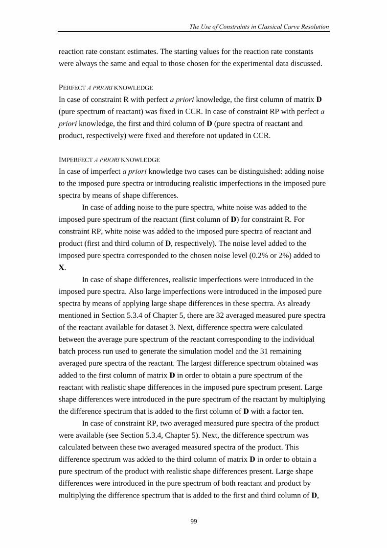
99

reaction rate constant estimates. The starting values for the reaction rate constants

were always the same and equal to those chosen for the experimental data discussed.

PERFECT �� !�� KNOWLEDGE

In case of constraint R with perfect �� knowledge, the first column of matrix �

(pure spectrum of reactant) was fixed in CCR. In case of constraint RP with perfect �

�� knowledge, the first and third column of � (pure spectra of reactant and

product, respectively) were fixed and therefore not updated in CCR.

IMPERFECT �� !�� KNOWLEDGE

In case of imperfect �� knowledge two cases can be distinguished: adding noise

to the imposed pure spectra or introducing realistic imperfections in the imposed pure

spectra by means of shape differences.

In case of adding noise to the pure spectra, white noise was added to the

imposed pure spectrum of the reactant (first column of �) for constraint R. For

constraint RP, white noise was added to the imposed pure spectra of reactant and

product (first and third column of �, respectively). The noise level added to the

imposed pure spectra corresponded to the chosen noise level (0.2% or 2%) added to

�.

In case of shape differences, realistic imperfections were introduced in the

imposed pure spectra. Also large imperfections were introduced in the imposed pure

spectra by means of applying large shape differences in these spectra. As already

mentioned in Section 5.3.4 of Chapter 5, there are 32 averaged measured pure spectra

of the reactant available for dataset 3. Next, difference spectra were calculated

between the average pure spectrum of the reactant corresponding to the individual

batch process run used to generate the simulation model and the 31 remaining

averaged pure spectra of the reactant. The largest difference spectrum obtained was

added to the first column of matrix � in order to obtain a pure spectrum of the

reactant with realistic shape differences in the imposed pure spectrum present. Large

shape differences were introduced in the pure spectrum of the reactant by multiplying

the difference spectrum that is added to the first column of � with a factor ten.

In case of constraint RP, two averaged measured pure spectra of the product

were available (see Section 5.3.4, Chapter 5). Next, the difference spectrum was

calculated between these two averaged measured spectra of the product. This

difference spectrum was added to the third column of matrix � in order to obtain a

pure spectrum of the product with realistic shape differences present. Large shape

differences were introduced in the pure spectrum of both reactant and product by

multiplying the difference spectrum that is added to the first and third column of �,

��

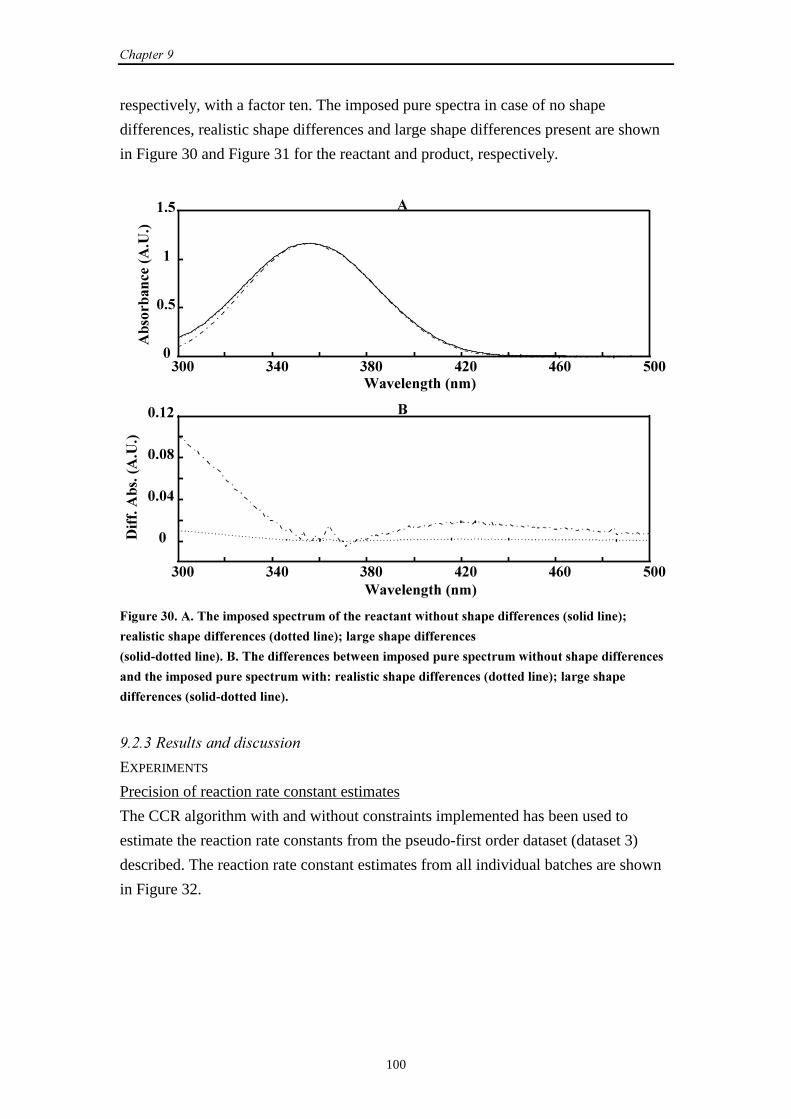
100

respectively, with a factor ten. The imposed pure spectra in case of no shape

differences, realistic shape differences and large shape differences present are shown

in Figure 30 and Figure 31 for the reactant and product, respectively.

!! "! #! "�! "$! %!!!

!�%

�

��%

!! "! #! "�! "$! %!!

!

!�!"

!�!#

!��

&��'��(�)*

&��'��(�)*

��+,��(+��*

+,� �,�

��(+

��*

+

-

��'�� !��+��)� ��)� ��.�� (� ��*/

��(� ��*/��'��

(� �� *��-��,��.��)� ��)�.��

��)� ��)�.��0��(� ��*/��'��

��(� �� *�

��"��

EXPERIMENTS

Precision of reaction rate constant estimates

The CCR algorithm with and without constraints implemented has been used to

estimate the reaction rate constants from the pseudo-first order dataset (dataset 3)

described. The reaction rate constant estimates from all individual batches are shown

in Figure 32.

��

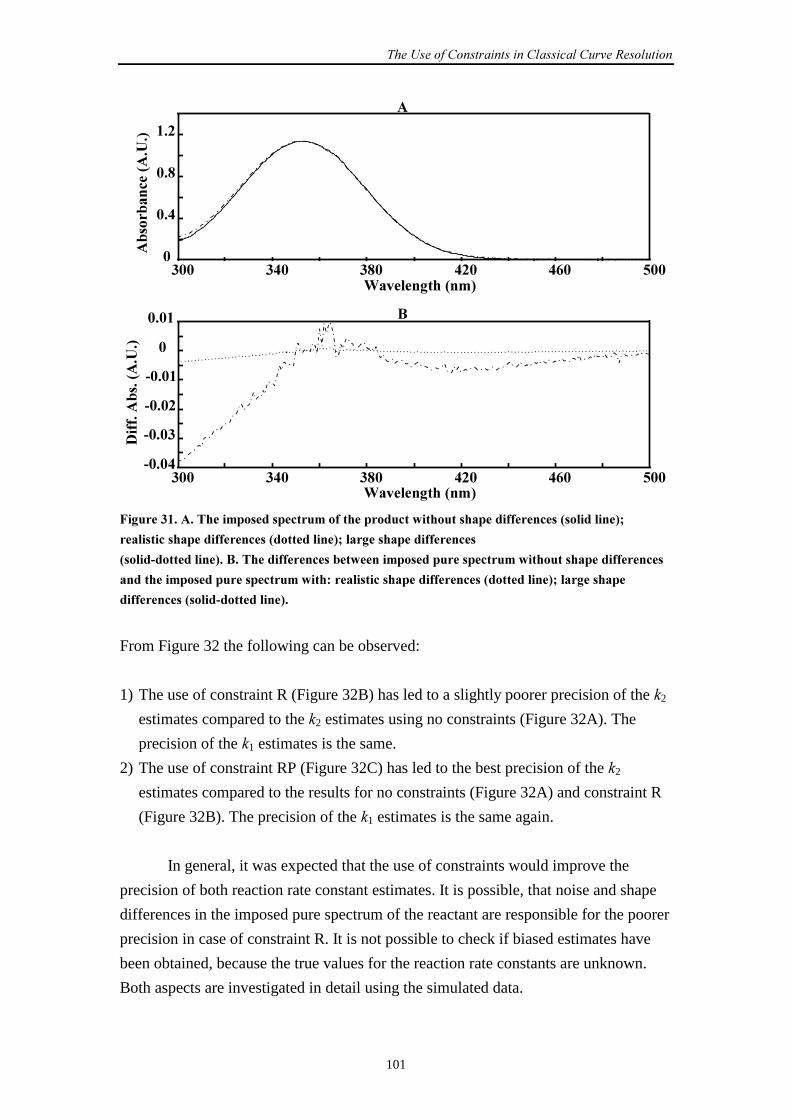
101

!! "! #! "�! "$! %!!!

!�"

!�#

��

!! "! #! "�! "$! %!!�!�!"

�!�!

�!�!�

�!�!�

!

!�!�

&��'��(�)*

&��'��(�)*

��+,��(+��*

+

-

+,� �,�

��(+

��*

��'�� +��)� ��)� �� .�� (� ��*/

��(� ��*/��'��

(� �� *��-��,��.��)� ��)�.��

��)� ��)�.��0��(� ��*/��'��

��(� �� *�

From Figure 32 the following can be observed:

1) The use of constraint R (Figure 32B) has led to a slightly poorer precision of the �2

estimates compared to the �2 estimates using no constraints (Figure 32A). The

precision of the �1 estimates is the same.

2) The use of constraint RP (Figure 32C) has led to the best precision of the �2

estimates compared to the results for no constraints (Figure 32A) and constraint R

(Figure 32B). The precision of the �1 estimates is the same again.

In general, it was expected that the use of constraints would improve the

precision of both reaction rate constant estimates. It is possible, that noise and shape

differences in the imposed pure spectrum of the reactant are responsible for the poorer

precision in case of constraint R. It is not possible to check if biased estimates have

been obtained, because the true values for the reaction rate constants are unknown.

Both aspects are investigated in detail using the simulated data.

��

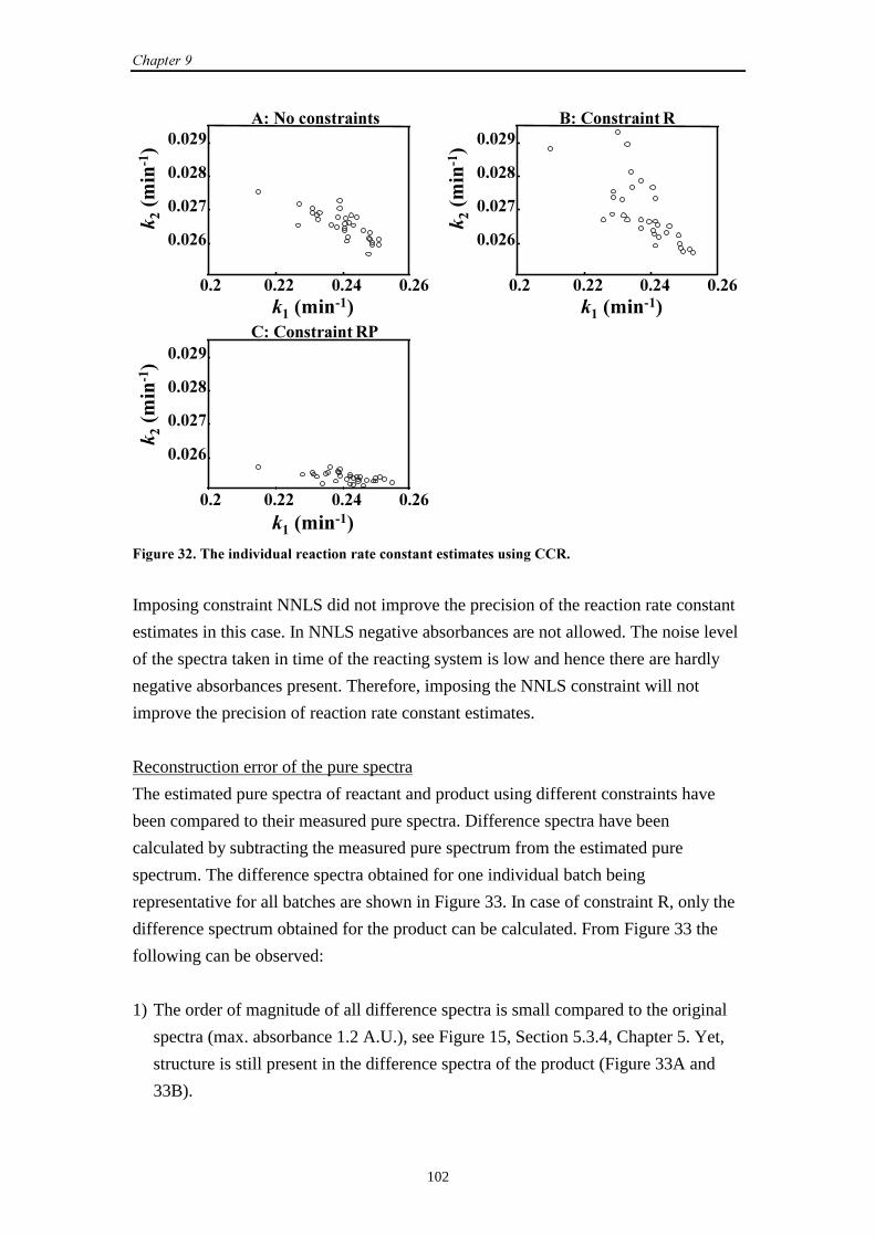
102

!�� !�� !��" !��$

!�!�$

!�!�1

!�!�#

!�!�+0�2 ��

!�� !�� !��" !��$

!�!�$

!�!�1

!�!�#

!�!�-0��

�

�

!�� !�� !��" !��$

!�!�$

!�!�1

!�!�#

!�!��0��

�

�3

� ��()��

��*

��()��*

� ��()��

��*

��()��*

� ��()��

��*

��()��*

��'�� )��'��

Imposing constraint NNLS did not improve the precision of the reaction rate constant

estimates in this case. In NNLS negative absorbances are not allowed. The noise level

of the spectra taken in time of the reacting system is low and hence there are hardly

negative absorbances present. Therefore, imposing the NNLS constraint will not

improve the precision of reaction rate constant estimates.

Reconstruction error of the pure spectra

The estimated pure spectra of reactant and product using different constraints have

been compared to their measured pure spectra. Difference spectra have been

calculated by subtracting the measured pure spectrum from the estimated pure

spectrum. The difference spectra obtained for one individual batch being

representative for all batches are shown in Figure 33. In case of constraint R, only the

difference spectrum obtained for the product can be calculated. From Figure 33 the

following can be observed:

1) The order of magnitude of all difference spectra is small compared to the original

spectra (max. absorbance 1.2 A.U.), see Figure 15, Section 5.3.4, Chapter 5. Yet,

structure is still present in the difference spectra of the product (Figure 33A and

33B).

��

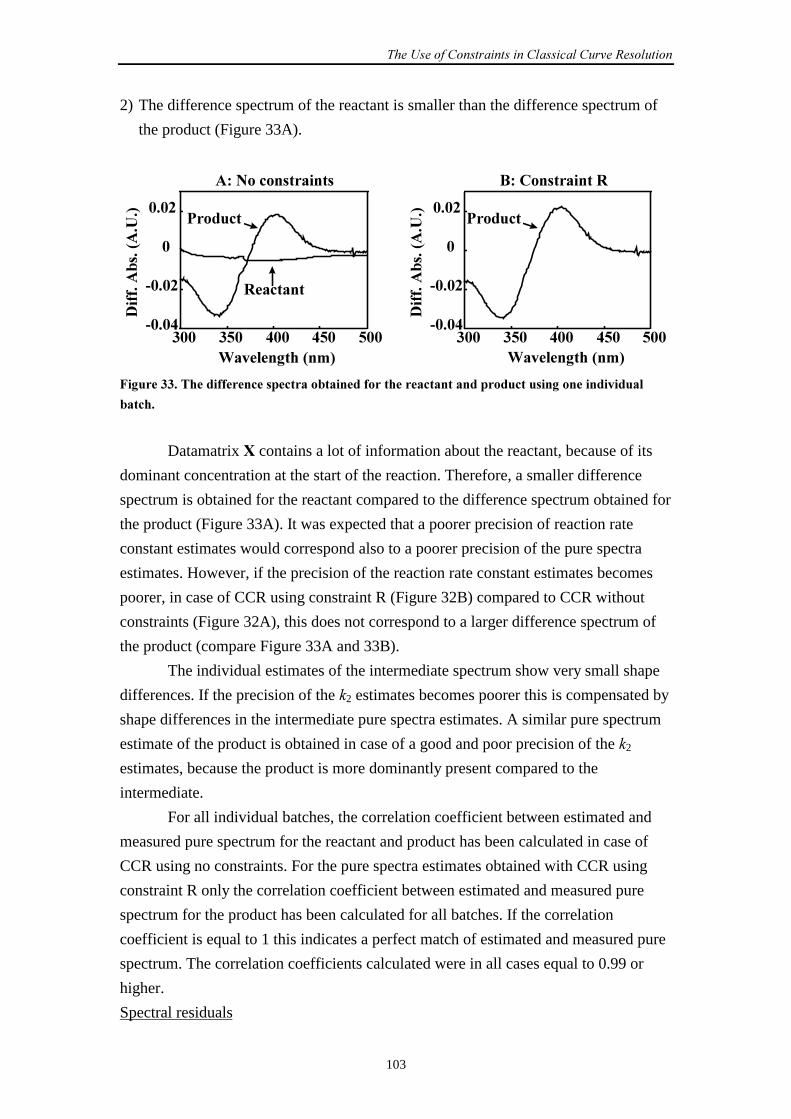
103

2) The difference spectrum of the reactant is smaller than the difference spectrum of

the product (Figure 33A).

!! %! "!! "%! %!!�!�!"

�!�!�

!

!�!�

!! %! "!! "%! %!!�!�!"

�!�!�

!

!�!�

&��'��(�)* &��'��(�)*

��+,��(+��*

��+,��(+��*

��

3� �� 3� ��

+0�2 �� -0��

��'�� ,�� '� ��

,��

Datamatrix � contains a lot of information about the reactant, because of its

dominant concentration at the start of the reaction. Therefore, a smaller difference

spectrum is obtained for the reactant compared to the difference spectrum obtained for

the product (Figure 33A). It was expected that a poorer precision of reaction rate

constant estimates would correspond also to a poorer precision of the pure spectra

estimates. However, if the precision of the reaction rate constant estimates becomes

poorer, in case of CCR using constraint R (Figure 32B) compared to CCR without

constraints (Figure 32A), this does not correspond to a larger difference spectrum of

the product (compare Figure 33A and 33B).

The individual estimates of the intermediate spectrum show very small shape

differences. If the precision of the �2 estimates becomes poorer this is compensated by

shape differences in the intermediate pure spectra estimates. A similar pure spectrum

estimate of the product is obtained in case of a good and poor precision of the �2

estimates, because the product is more dominantly present compared to the

intermediate.

For all individual batches, the correlation coefficient between estimated and

measured pure spectrum for the reactant and product has been calculated in case of

CCR using no constraints. For the pure spectra estimates obtained with CCR using

constraint R only the correlation coefficient between estimated and measured pure

spectrum for the product has been calculated for all batches. If the correlation

coefficient is equal to 1 this indicates a perfect match of estimated and measured pure

spectrum. The correlation coefficients calculated were in all cases equal to 0.99 or

higher.

Spectral residuals

��

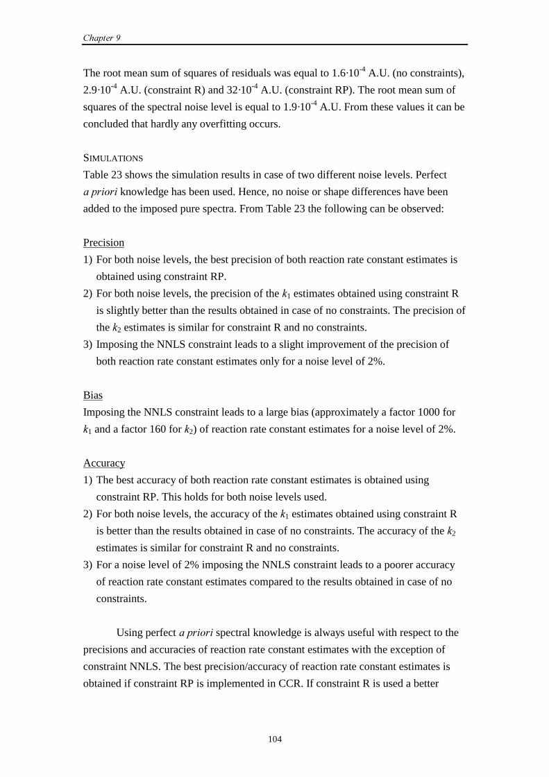
104

The root mean sum of squares of residuals was equal to 1.6·10-4 A.U. (no constraints),

2.9·10-4 A.U. (constraint R) and 32·10-4 A.U. (constraint RP). The root mean sum of

squares of the spectral noise level is equal to 1.9·10-4 A.U. From these values it can be

concluded that hardly any overfitting occurs.

SIMULATIONS

Table 23 shows the simulation results in case of two different noise levels. Perfect

�� knowledge has been used. Hence, no noise or shape differences have been

added to the imposed pure spectra. From Table 23 the following can be observed:

Precision

1) For both noise levels, the best precision of both reaction rate constant estimates is

obtained using constraint RP.

2) For both noise levels, the precision of the �1 estimates obtained using constraint R

is slightly better than the results obtained in case of no constraints. The precision of

the �2 estimates is similar for constraint R and no constraints.

3) Imposing the NNLS constraint leads to a slight improvement of the precision of

both reaction rate constant estimates only for a noise level of 2%.

Bias

Imposing the NNLS constraint leads to a large bias (approximately a factor 1000 for

�1 and a factor 160 for �2) of reaction rate constant estimates for a noise level of 2%.

Accuracy

1) The best accuracy of both reaction rate constant estimates is obtained using

constraint RP. This holds for both noise levels used.

2) For both noise levels, the accuracy of the �1 estimates obtained using constraint R

is better than the results obtained in case of no constraints. The accuracy of the �2

estimates is similar for constraint R and no constraints.

3) For a noise level of 2% imposing the NNLS constraint leads to a poorer accuracy

of reaction rate constant estimates compared to the results obtained in case of no

constraints.

Using perfect �� spectral knowledge is always useful with respect to the

precisions and accuracies of reaction rate constant estimates with the exception of

constraint NNLS. The best precision/accuracy of reaction rate constant estimates is

obtained if constraint RP is implemented in CCR. If constraint R is used a better

��

105

�,�� 4�)�� (� ��*��

5� .��'��. �� ,��.��

�� )��

Constr. Noise

level

(%)

Precision

�1 ·10-9

(min-1)2

Precision

�2 ·10-9

(min-1)2

Bias

�1 ·10-9

(min-1)2

Bias

�2 ·10-9

(min-1)2

Accuracy

�1 ·10-9

(min-1)2

Accuracy

�2 ·10-9

(min-1)2

none 0.2 20 3 < 1 < 1 20

(<1%)

3

(<1%)

R 0.2 12 3 < 1 < 1 12

(<1%)

3

(<1%)

RP 0.2 4 < 1 < 1 < 1 4

(<1%)

< 1

(<1%)

NNLS 0.2 20 3 < 1 < 1 20

(<1%)

3

(<1%)

none 2 1973 257 1 < 1 1974

(<1%)

257

(<1%)

R 2 1169 227 7 1 1176

(<1%)

228

(<1%)

RP 2 345 3 2 < 1 347

(<1%)

3

(<1%)

NNLS 2 1383 150 1030 162 2413

(<1%)

312

(2%)

precision/accuracy for �1 is obtained compared to the results in case of no constraints

and a poorer precision/accuracy is obtained compared to the results for constraint RP.

Datamatrix � contains less information about the product (low selectivity) compared

to the reactant and there is a large spectral overlap present between the pure spectrum

of the reactant and product. Hence, imposing constraint RP will result in a large gain

in precision/accuracy of reaction rate constant estimates.

A higher noise level of the spectral data results in a large bias if constraint

NNLS is imposed. An explanation for this is the existence of negative absorbances in

the spectra taken in time of the reaction mixture. In NNLS negative absorbances are

not allowed. This means that an offset is introduced in the data which may result in a

bias dependent on the order of magnitude of the offset.

Table 24 shows the simulation results using imperfect �� knowledge and

two different noise levels. Noise has been added to the imposed pure spectra of the

reacting absorbing species. From Table 24, the following can be observed:

Precision

��

106

1) For both noise levels, the use of constraint R or constraint RP leads to a poorer

precision of reaction rate constant estimates compared to the precision in case of

unconstrained CCR. However, there is one exception. For a noise level of 2%, the

use of constraint RP leads to a better precision for �2 compared to unconstrained

CCR.

2) Again, for both noise levels, the use of constraint RP gives a better precision of

reaction rate constant estimates compared to the precision obtained for constraint R

(approximately a factor two for �1 and a factor eight for �2).

Bias

1) In all cases a large bias (≥1%) is obtained compared to unconstrained CCR.

2) For both noise levels, the use of constraint R has led to a smaller bias for �1

compared to the bias for �1 in case of constraint RP. However, the opposite is

observed for �2.

3) For the two noise levels used the bias of reaction rate constant estimates is almost

independent of these noise levels.

Accuracy

1) For both noise levels, the use of constraint RP only gives a better accuracy of �2

compared to the accuracy obtained for constraint R.

2) For both noise levels, the use of constraint R has led to a dramatic poor accuracy of

the reaction rate constant estimates compared to the accuracy in case of

unconstrained CCR.

3) For a noise level of 2%, the accuracy is improved for �2 if constraint RP is used

compared to unconstrained CCR.

The use of constraint RP gives only a better accuracy of �2, because this reaction rate

constant is directly connected to the product. Hence, imposing product information

will influence mainly the �2 estimates.

It is obvious that imposing constraints based on the use of imperfect ��

knowledge (noise added to pure spectra) must be avoided. The accuracy of reaction

rate constant estimates obtained is independent of both noise levels used. In all cases

imposing noisy pure spectra results in biased reaction rate constant estimates.

�,��"��4�)�� (� ��*�� )��

5� .��'��. �� 2 ��,��

��

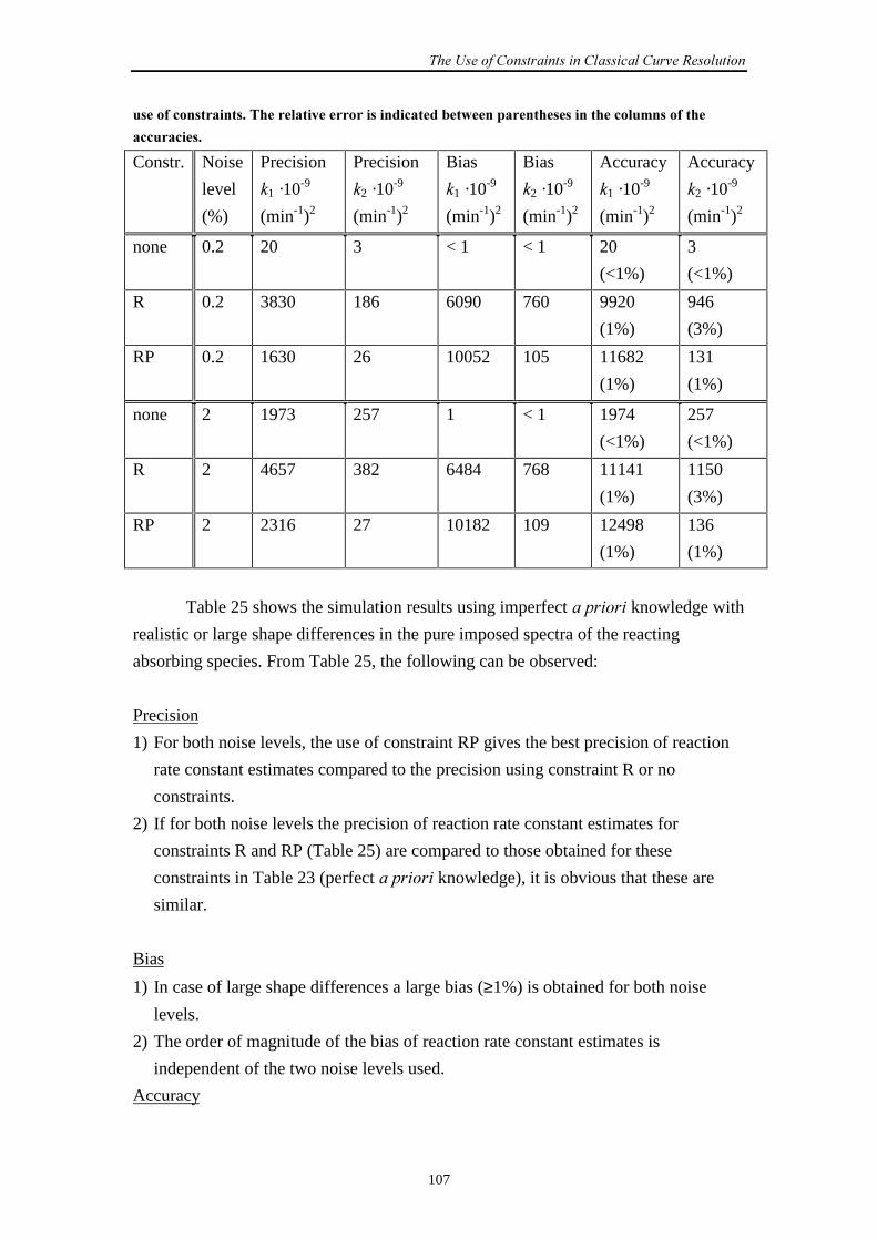
107

�� ,��.�� )��

��

Constr. Noise

level

(%)

Precision

�1 ·10-9

(min-1)2

Precision

�2 ·10-9

(min-1)2

Bias

�1 ·10-9

(min-1)2

Bias

�2 ·10-9

(min-1)2

Accuracy

�1 ·10-9

(min-1)2

Accuracy

�2 ·10-9

(min-1)2

none 0.2 20 3 < 1 < 1 20

(<1%)

3

(<1%)

R 0.2 3830 186 6090 760 9920

(1%)

946

(3%)

RP 0.2 1630 26 10052 105 11682

(1%)

131

(1%)

none 2 1973 257 1 < 1 1974

(<1%)

257

(<1%)

R 2 4657 382 6484 768 11141

(1%)

1150

(3%)

RP 2 2316 27 10182 109 12498

(1%)

136

(1%)

Table 25 shows the simulation results using imperfect �� knowledge with

realistic or large shape differences in the pure imposed spectra of the reacting

absorbing species. From Table 25, the following can be observed:

Precision

1) For both noise levels, the use of constraint RP gives the best precision of reaction

rate constant estimates compared to the precision using constraint R or no

constraints.

2) If for both noise levels the precision of reaction rate constant estimates for

constraints R and RP (Table 25) are compared to those obtained for these

constraints in Table 23 (perfect �� knowledge), it is obvious that these are

similar.

Bias

1) In case of large shape differences a large bias (≥1%) is obtained for both noise

levels.

2) The order of magnitude of the bias of reaction rate constant estimates is

independent of the two noise levels used.

Accuracy

��

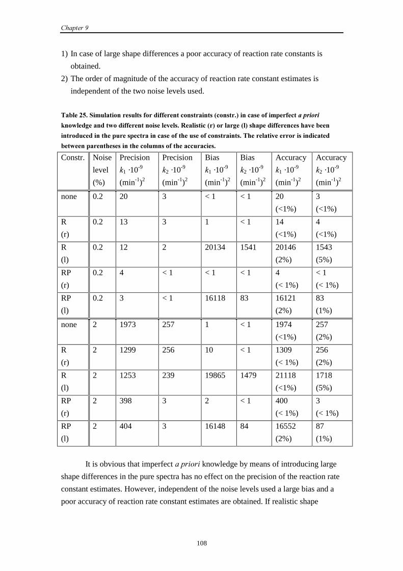
108

1) In case of large shape differences a poor accuracy of reaction rate constants is

obtained.

2) The order of magnitude of the accuracy of reaction rate constant estimates is

independent of the two noise levels used.

�,��%��4�)�� (� ��*�� )��

5� .��'��. �� (�*� ��'��(�*��,��

��

,��.�� )��

Constr. Noise

level

(%)

Precision

�1 ·10-9

(min-1)2

Precision

�2 ·10-9

(min-1)2

Bias

�1 ·10-9

(min-1)2

Bias

�2 ·10-9

(min-1)2

Accuracy

�1 ·10-9

(min-1)2

Accuracy

�2 ·10-9

(min-1)2

none 0.2 20 3 < 1 < 1 20

(<1%)

3

(<1%)

R

(r)

0.2 13 3 1 < 1 14

(<1%)

4

(<1%)

R

(l)

0.2 12 2 20134 1541 20146

(2%)

1543

(5%)

RP

(r)

0.2 4 < 1 < 1 < 1 4

(< 1%)

< 1

(< 1%)

RP

(l)

0.2 3 < 1 16118 83 16121

(2%)

83

(1%)

none 2 1973 257 1 < 1 1974

(<1%)

257

(2%)

R

(r)

2 1299 256 10 < 1 1309

(< 1%)

256

(2%)

R

(l)

2 1253 239 19865 1479 21118

(<1%)

1718

(5%)

RP

(r)

2 398 3 2 < 1 400

(< 1%)

3

(< 1%)

RP

(l)

2 404 3 16148 84 16552

(2%)

87

(1%)

It is obvious that imperfect �� knowledge by means of introducing large

shape differences in the pure spectra has no effect on the precision of the reaction rate

constant estimates. However, independent of the noise levels used a large bias and a

poor accuracy of reaction rate constant estimates are obtained. If realistic shape

��

109

differences are introduced, which are representative for the experiments performed,

the precision, bias and accuracy are not affected.

Summary of the simulation results

In case of perfect �� knowledge applying constraints leads to better precisions

and accuracies of reaction rate constant estimates. If noise is added to the imposed

pure spectra, which results in imperfect �� knowledge, the precisions and

accuracies of reaction rate constant estimates become poorer. However, there is one

exception. For a noise level of 2%, the precision and accuracy of the �2 estimates is

improved if constraint RP is used compared to unconstrained CCR. If imperfect

knowledge is present in the form of realistic or large shape differences in the pure

spectra, the precisions of reaction rate constant estimates are similar compared to

those obtained in case of perfect �� knowledge. Hence, the precision is mainly

affected by the presence of noise on the imposed pure spectra.

In case of a high noise level and perfect �� knowledge, imposing the

NNLS constraint gives a large bias for both reaction rate constant estimates due to

negative absorbances present in the spectral data. If imperfect �� knowledge is

used (noise or large shape differences added to the imposed pure spectra), a large bias

of reaction rate constant estimates can be obtained. The order of magnitude of the bias

of reaction rate constant estimates is independent of the two noise levels used in this

study. No bias is obtained in case of realistic shape differences introduced in the

imposed pure spectra.

Spectral residuals

For the results of the simulations, spectral residuals have been inspected. In all cases

(perfect and imperfect �� knowledge) the spectral residuals represented white

noise except for imperfect �� knowledge where large shape differences have

been introduced in the pure spectra. Hence, it might be claimed that structure in the

residuals is an indication of the quality of the �� incorporated spectra.

In Figure 34, the spectral residuals are shown for one batch process of the

experimental dataset (dataset 3) in case of unconstrained CCR. The two largest

spectral residual spectra are the first two spectral residual spectra of the batch process.

The spectral residuals for other batches were similar. The residuals show some

structure, which can be caused by spectral characteristics like drift, non-uniform errors

and coloured noise. Hence, spectral residuals are not good indicators for the quality of

the �� imposed pure spectra, because in the residuals of unconstrained CCR

there is already structure present. In case of unconstrained CCR, a comparison of pure

spectra estimates and measured pure spectra can serve as a diagnostic tool.

��

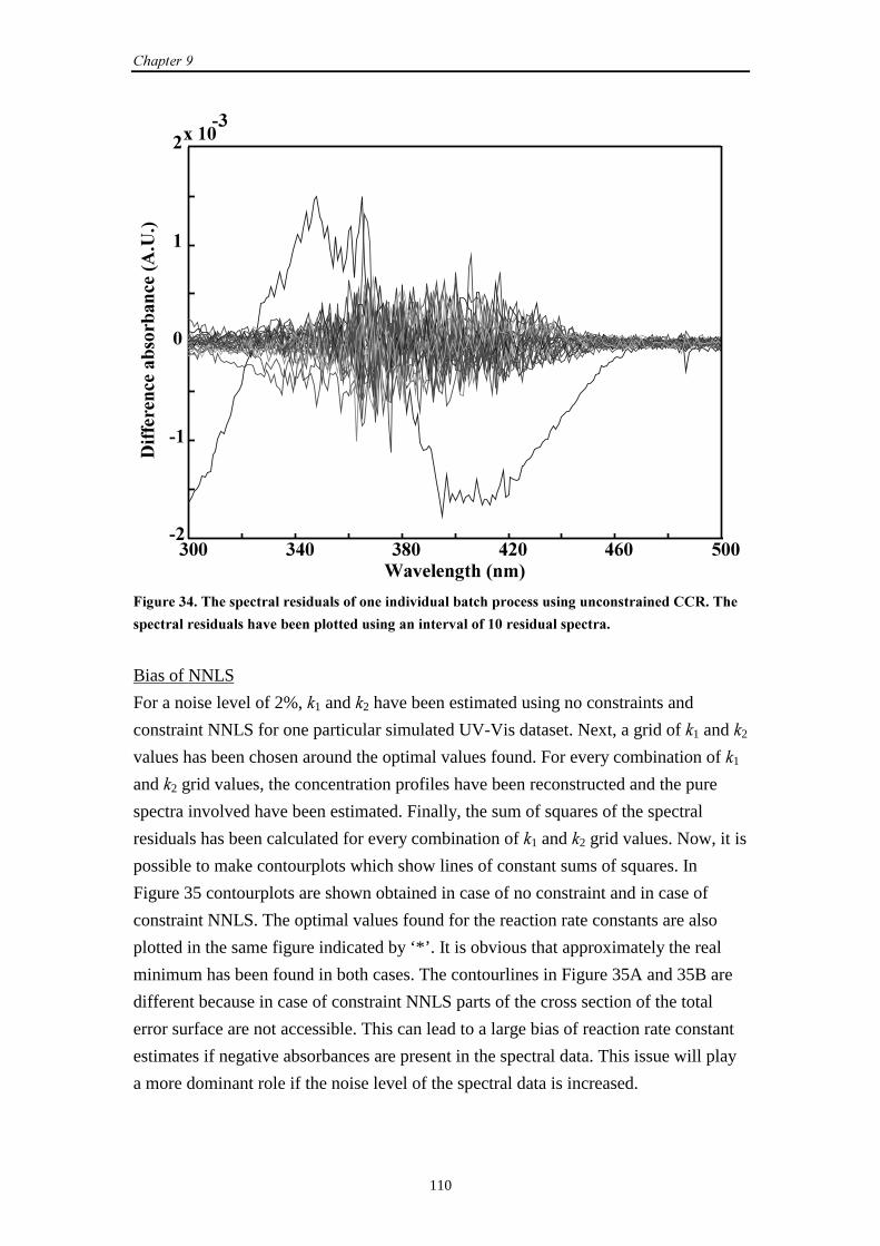
110

!! "! #! "�! "$! %!!��

��

!

�

�6��!�

&��'��(�)*

��,

� �,��

��(+��*

��'�� "�� ,�� '��

��,�� '�� !��

Bias of NNLS

For a noise level of 2%, �1 and �2 have been estimated using no constraints and

constraint NNLS for one particular simulated UV-Vis dataset. Next, a grid of �1 and �2

values has been chosen around the optimal values found. For every combination of �1

and �2 grid values, the concentration profiles have been reconstructed and the pure

spectra involved have been estimated. Finally, the sum of squares of the spectral

residuals has been calculated for every combination of �1 and �2 grid values. Now, it is

possible to make contourplots which show lines of constant sums of squares. In

Figure 35 contourplots are shown obtained in case of no constraint and in case of

constraint NNLS. The optimal values found for the reaction rate constants are also

plotted in the same figure indicated by ‘*’. It is obvious that approximately the real

minimum has been found in both cases. The contourlines in Figure 35A and 35B are

different because in case of constraint NNLS parts of the cross section of the total

error surface are not accessible. This can lead to a large bias of reaction rate constant

estimates if negative absorbances are present in the spectral data. This issue will play

a more dominant role if the noise level of the spectral data is increased.

��

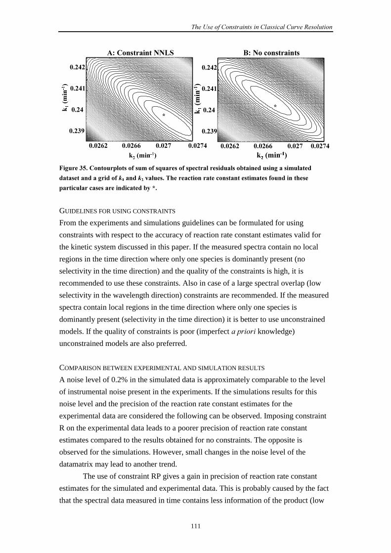
111

!�!�$� !�!�$$ !�!�1 !�!�1"

!��

!��"

!��"�

!��"�

!�!�$� !�!�$$ !�!�1 !�!�1"

!��

!��"

!��"�

!��"�5 �

�()��

��

*

5��()��* 5

��()��*

5 �

�()��

��

*

+0�� 2274 -0�2 ��

88

��'�� %�� )� ��9�� ,��'��)��

��'�� )��

��,:�8�

GUIDELINES FOR USING CONSTRAINTS

From the experiments and simulations guidelines can be formulated for using

constraints with respect to the accuracy of reaction rate constant estimates valid for

the kinetic system discussed in this paper. If the measured spectra contain no local

regions in the time direction where only one species is dominantly present (no

selectivity in the time direction) and the quality of the constraints is high, it is

recommended to use these constraints. Also in case of a large spectral overlap (low

selectivity in the wavelength direction) constraints are recommended. If the measured

spectra contain local regions in the time direction where only one species is

dominantly present (selectivity in the time direction) it is better to use unconstrained

models. If the quality of constraints is poor (imperfect �� knowledge)

unconstrained models are also preferred.

COMPARISON BETWEEN EXPERIMENTAL AND SIMULATION RESULTS

A noise level of 0.2% in the simulated data is approximately comparable to the level

of instrumental noise present in the experiments. If the simulations results for this

noise level and the precision of the reaction rate constant estimates for the

experimental data are considered the following can be observed. Imposing constraint

R on the experimental data leads to a poorer precision of reaction rate constant

estimates compared to the results obtained for no constraints. The opposite is

observed for the simulations. However, small changes in the noise level of the

datamatrix may lead to another trend.

The use of constraint RP gives a gain in precision of reaction rate constant

estimates for the simulated and experimental data. This is probably caused by the fact

that the spectral data measured in time contains less information of the product (low

��

112

selectivity) and a large spectral overlap of the pure spectrum of the reactant and the

product is present.

��#��

In this Chapter, the usefulness of constraints in CCR for improving the accuracy of

rate constant estimates from kinetic data has been investigated. From the results

obtained from dataset 3 it can be concluded that the precision of the reaction rate

constant estimates is the best if the �� known pure spectra of both reactant and

product are implemented as constraints in CCR. The presence of biased estimates of

reaction rate constants could not be checked.

In order to investigate if biased reaction rate constant estimates are obtained

using CCR with and without constraints implemented, simulations have been set up

so that the simulated UV-Vis spectra looked very similar to the experimental spectra.

Using perfect �� knowledge improved the precisions and accuracies of reaction

rate constant estimates. However, imposing noisy pure spectra (imperfect ��

knowledge) resulted in a poor precisions and accuracies of reaction rate constant

estimates. Moreover, a large bias of reaction rate constant estimates is obtained. In

case of imposing imperfect �� knowledge by means of introducing large shape

differences in the pure spectra a large bias of reaction rate constants is obtained, but

the precision is not affected.

From the results of the simulated data, guidelines have been formulated for the

use of constraints with respect to the accuracy of reaction rate constants valid for the

kinetic system discussed in this paper. If the measured spectra contain no local regions

in the time direction where only one species is dominantly present (low selectivity)

and the quality of the constraints is high it is useful to impose the constraints. Also in

case of a large spectral overlap it is useful to apply constraints. If the measured spectra

contain local regions in the time direction where only one species is dominantly

present (high selectivity) it is better to use unconstrained models. It is also better to

use unconstrained models if the quality of constraints is poor (imperfect ��

knowledge). In practice, a better precision obtained for experimental data is no good

reason to use constraints. The true values of the reaction rate constants of interest are

always unknown. This makes it difficult to check if biased reaction rate constant

estimates have been obtained.

113

��

��

��

In this thesis, modified curve resolution based methods (two-way methods) and

three-way methods are presented to estimate reaction rate constants from chemical

reactions. Applications of the two-way and three-way methods described in this thesis,

show the applicability of these methods for estimating reaction rate constants from

spectroscopic data of time evolving chemical systems. Attention is paid to the use of

constraints implemented in two-way and three-way methods. ��

��

��

��

��

�� From the work reported, some conclusions can be summarized.

��

� A combination of fixed-size window evolving factor analysis (FSWEFA) and

traditional curve fitting (TCF) has resulted in a method for estimating reaction rate

constants from spectroscopic data based on wavelength selection (��

and ��, ��). This approach is superior to full wavelength two-way

methods in case of spectral data where the absorbance differences in time of the

species of interest, from which the reaction rate constants are estimated, are large

and a good selective window exists (��, ��).

� The two-way methods are suitable for �-th order kinetics (�� and �).

� If two-way methods are considered, the use of �� spectral information is only

possible in case of classical curve resolution (CCR) (��).

� CCR with �� spectral information implemented gives the best precision of

reaction rate constant estimates compared to other two-way methods (��

and �).

��

114

��

� The precision of reaction rate constant estimates is affected by the choice of the

applied time shift or step-size (�� and �).

� The generalized rank annihilation method (GRAM) and the trilinear decomposition

method (TLD) can both have many future applications in the field of process

monitoring and control because of the fast and non-iterative nature of the

algorithms (�� and �).

� Three-way methods are only applicable for (pseudo-) first order kinetics

(��, � and �).

��

� In case of spectroscopic data with a moderate signal to noise ratio present, two-way

methods are preferred instead of three-way methods. Two-way methods give an

acceptable precision of reaction rate constant estimates (��).

� In case of spectroscopic data with a high signal to noise ratio present, two-way

methods and three-way methods perform the same. These methods give similar

precisions of reaction rate constant estimates (��). The three-way methods

GRAM and TLD are preferred, because of their fast performance and non-iterative

nature. However, it is unkown if biased estimates are obtained in this case using

two-way and three-way methods.

��

� For experimental data, the best precision of reaction rate constant estimates is

obtained if �� spectral information is implemented in CCR (��, �

and �). However, it is never possible in practice to check if biased estimates have

been obtained.

� Simulations proved that an improvement of the precision of reaction rate constant

estimates can be associated with the presence of biased estimates. Hence, the use of

constraints within CCR is not always recommended (��). If a high

selectivity of species is present in time it is better to use unconstrained models. In

case of a low selectivity of species in time or a large spectral overlap of some of the

pure spectra of the reacting absorbing species, it is useful to apply constrained

models if the quality of the constraints is high.

��

� For the application of three-way methods in practice, the choice of the order of

magnitude of the column with constants that has to be added to the spectral

datamatrix is a very important constraint that has to be implemented in the

�� !��

115

non-least squares methods GRAM and TLD (��, � and �).

��

From the results reported in this thesis, it is obvious that some aspects have to be

investigated further in detail.

��

In �� and ��, the theory and applications of two-way methods have

been discussed, respectively. In ��, the use of constraints within the two-way

method CCR has been discussed very extensively. However, further research is

necessary to investigate the impact of the use of constraint P and penalty functions1 on

the precision of reaction rate constant estimates. With the aid of simulated data

imposing perfect and imperfect �� knowledge it is worthwhile to investigate if

this may lead to biased estimates. The use of �� known pure spectra within

iterative three-way methods and the effect on the precision, bias and accuracy of

reaction rate constant estimates must be investigated in the future. Attention should be

payed to the comparison between constrained and unconstrained three-way models.

�"#$

In general, it is very interesting to investigate GRAM (��, � and �) in more

detail. This method is based on the principle that the reaction rate constant of interest

can be extracted immediately from the ratio of the equation of the concentration

profile and the equation of the time shifted concentration profile. The manner in

which two slabs are created from one spectral dataset using GRAM can also be done

in another way. For example, the first slab can be created from the spectra measured at

odd time points and the second slab can be created from the spectra measured at even

time points. It may be worthwhile, to find a procedure to split the spectral dataset in

such a way that the precision of the reaction rate constant estimates is the best and no

biased estimates are obtained. Faber ��.2 wrote a paper about the derivation of

expressions for predicting the bias and the variance in the eigenvalues obtained with

GRAM. Maybe it is possible to correct for biased estimates.

$�� %$�"&

In multivariate curve resolution (MCR) the spectral data of several experiments are

analyzed simultaneously. This can be an advantage with respect to noise reduction and

improving the accuracy of reaction rate constant estimates. Hence, MCR is an

interesting approach which is also possible in multiway analysis. In this way it is also

��

116

feasible to analyze pseudo-first order and second order spectral kinetic data

simultaneously by means of stacking multiple two-way datasets.

'��

A whole new area in the field of kinetics could be the on-line monitoring of reaction

rate constants combined with process control. Using tools from multivariate statistical

process control may help to achieve this goal.

��!�"��1. Lee S-Y. ‘Estimation of covariance structure models with parameters subject to functional restraints’.

( ��, 1980; �#: 309-324.

2. Faber K, Lorber A, Kowalski BR. ‘Generalized rank annihilation method: Standard errors in the

estimated eigenvalues of the instrumental errors are heteroscedastic and correlated’.

)�� , 1997; : 95-110.

117

��

��

��

Dataset 1 contains SW-NIR spectra taken in time of the two-step consecutive

epoxidation of 2,5-di-��-butyl-1,4-benzoquinone using ��-butyl hydroperoxide and

Triton B catalyst. The reaction consists of the following two steps:

+ → DN � + �

� + → EN + �

with second order reaction rate constants �a and �b both in M-1min-1. If species is

present in large excess, the first and second reaction step become both pseudo-first

order reactions with pseudo-first order reaction rate constants �1 (min-1) and �2 (min-1),

respectively. Species , �, and are spectroscopically active. The experiment was

repeated eight times under identical pseudo-first order conditions.

��

Dataset 2 contains UV-Vis spectra of the two-step consecutive reaction of

3-chlorophenylhydrazonopropane dinitrile with 2-mercaptoethanol. The reaction

consists of the following two steps:

+ → DN �

� → 2N + �

with second order reaction rate constant �a (M-1min-1) and first order reaction rate

constant �2 (min-1). If species is present in large excess the first step of the reaction

becomes pseudo-first order with pseudo-first order reaction rate constant �1 (min-1).

Species , �, and are spectroscopically active. The experiment was repeated ten

times under identical pseudo-first order conditions at a pH of 5.4.

��

Dataset 3 contains spectra taken in time of the same reaction as in case of dataset 2.

However, in case of dataset 3 the experiment was repeated 32 times under identical

pseudo-first order conditions at a pH of 5.2.

��

��

118

Dataset 4 contains spectra taken in time of the same reaction as in case of dataset 2.

However, in case of dataset 4, the first reaction is performed under second order

conditions. A pH of 5.2 was used, the same pH that is valid for dataset 3. In case of

dataset 4, the second order experiment was repeated six times for three different initial

concentrations of both reactants (species and species ). The ratio’s �8,0:�9,0 were

chosen equal to 1:4, 1:5 and 1:6. Hence, for a ratio of �8,0:�9,0 equal to 1:4, six

experiments were fulfilled. In total 18 second order experiments were performed.

��

��

In this Section,i a proof is given that a unique solution of the curve resolution model is

obtained in case of imposing a kinetic model in the curve resolution algorithm.

Consider matrix � from Equation (1), Section 2.2, Chapter 2. Consider also

Equation (6)-(8) from the same Section which describe the concentration profiles of

species , � and of the chemical reaction from Section 2.2 of Chapter 2. Matrix �

has a fixed structure, given the kinetic model, and depends only on �1 and �2. This will

be indicated as �(�1, �2). A simple basis � for the concentration profiles � in

Equation (1) can be found by defining � (Equation (51)) and � (Equation (52)):

�� WW ][ 21 NN −−= (51)

+=

12

1

12

1

12

1

12

1

-

-

- 0

1-

- -

1

1 0 0

��

��

��

��

� (52)

where it can be checked that � = ��. The notation W� UN− is shorthand for the vector

7WNWN 1UU �� ]..[ 1 −− where the time points �1, ..., �1 are the sampling points. The

structure of � and � are fixed. The elements of these matrices depend only on �1 and

i This Section is based on the following paper:

� Smilde AK, Hoefsloot HCJ, Bijlsma S, Boelens HFM. ‘Sufficient conditions for unique solutions

within a certain class of curve resolution models’. submitted.

��

119

�2. This will be indicated by � (�1, �2) and � (�1, �2). � is of full rank three (see later),

� is also of full rank (see Equation (52)), hence � is of full rank three.ii Therefore, the

columns of � are a basis for the column space of �.

If rotational freedom is present, then a (3x3) nonsingular � exists such that

�� = �* still has the structure of the kinetic model. This means that a �1* and �2*

should exist such that �� = � (�1*, �2*). Hence, �� = �� = � (�1*, �2*). Also,

�� = ��, where �� = � (�1*, �2*) and �� = � (�1*, �2*).

The transformation �� leaves the column-space of � intact, because � is

nonsingular. Now, � is a basis for the column-space of �, and likewise, �* is a basis

for the column-space of �� = ��. Therefore, � should also be a basis for the

column-space of ��. Hence, it should be possible to write all columns of �� as linear

combinations of the columns of �. Consider the columns WW ��*2

*1 and NN of ��. Later it is

shown that ][ 1 WW �� -NN −− forms a linear independent set for

�1 ≠ �2 ≠ ... ≠ �- and all �M > 0. Hence, the only solutions are: �1 = �1*, �2 = �2* or

�1 = �2*, �2 = �1*. The first solution means that there is no rotation possible, and the

second solution is simply a relabeling of the reaction constants. The latter can always

be checked by associating the constant related to the first profile in � to the first

reaction. Hence, in essence, rotational ambiguity is not present anymore.

The proof given above can be used for any kinetic model imposed on the data

where the matrix � is of full column-rank and each column of � can be written as a

linear combination of a basis ][ 21 WWW �� -NNN −−− . Of course, by extending �

with more columns, there are more labeling permutations possible, but these can be

resolved as commented above.

The intensity problem is trivially solved by imposing the kinetic model,

because all relative concentrations are imposed by the kinetic model. Providing the

algorithm with the correct starting concentrations gives then the unique intensities.

�� !��

It is shown that the exponential functions WN M�− (" = 1, ..., #; � ≥ 0) form a linear

independent set provided that �1 ≠ �2 ≠ ... ≠ �- and �M ≥ 0 for all ". In the following the

�1, ... �- will be ordered, without loss of generality, such that

�- > �-�� > ... > �1 ≥ 0. Consider the linear combination:

0;0...2121 ≥=⋅++⋅+⋅ −−− �� WN

-

WNWN - (53)

ii Schott JR. $��%�� &��, John Wiley & Sons: New York, 1997.

��

120

then it should follow that necessarily �1 = �2 = .. = �-�= 0. From Equation (54) follows

0)()...(0

2121 =+++∫

∞−−− �� WN

-

WNWN - (54)

which should hold for all functions f(�). By using )()( 1 ∞−= �� WN δ , where )( ∞−�δ

is the Dirac delta function,iii it holds that

0

0)()...(

0)()...(

0)()...(

1

0

)()(21

0

21

0

21

121

11211

121

=

⇒=∞−+++

⇒=∞−+++

⇒=∞−+++

∫

∫

∫

∞−−

∞−−−

∞−−−

�

��

��

��

WNN

-

WNN

WNWN

-

WNWNWNWN

WNWN

-

WNWN

-

-

-

δ

δ

δ

(55)

where the last step is true because if � approaches infinity, all terms in the summation

within the integral sign disappear except �1, which is a constant. Multiplied by

)( ∞−�δ the integral can only be zero if �1 = 0.

After having found that �1 = 0, the whole procedure can be repeated with

)()( 2 ∞−= �� WN δ and following the same reasoning as in Equation (55). This results

in �2 = 0. This procedure can be repeated for all terms in the linear combination of

Equation (53). Hence, all �j are necessarily zero and thus the functions powers of WN M�−

are linearly independent.

If the functions WN M�− are sampled in time, this will result in vectors7WNWN 1MM �� ]..[ 1 −− , with shorthand notation W� MN− . If the number of time points ' is

large enough (that is, ' ≥ #), then the resulting vectors W� MN− (" = 1, ..., #) are linearly

independent.

iii The Dirac delta function )( �� −δ is defined as ∞ for � = �, and 0 otherwise. Moreover,

.1)(0

=−∫∞

��δ

121

��

In this thesis, new two-way and three-way methods for estimating reaction rate

constants from spectroscopic measurements of chemical reactions are presented.

Applications of these methods to simulated and experimental data are reported.

In �� , a historical overview of chemical kinetics is given.

Experimental techniques, spectroscopy, multivariate analysis tools and the use of

constraints in kinetics are discussed. In �� , the goal and structure of the thesis

are also described.

In ��, the theory of the two-way methods traditional curve fitting

(TCF), classical curve resolution (CCR) and weighted curve resolution (WCR) is

described. In TCF reaction rate constants are estimated from the absorbance

differences in time (this is a concentration profile) of a certain species obtained from

one (or more) selective wavelength(s), that is (are) specific for mainly this species.

The unknown reaction rate constants are obtained by means of fitting the rate equation

of the specific species to the obtained concentration profile. It is important to stress

that TCF is an univariate method in case of one selective wavelength. Selective

wavelengths for the species of interest are obtained using fixed-size window evolving

factor analysis (FSWEFA), a local rank selection method.

Curve resolution is a set of techniques based on the determination of

qualitative information and the recovery of response profiles, for example time

profiles. If parameters of interest, for example reaction rate constants, are incorporated

as unknowns in curve resolution this results in modifications of curve resolution

techniques, because specific kinetic information is used explicitly. One of these

modifications is the CCR algorithm. In CCR, reaction rate constants and pure spectra

of reacting absorbing species are estimated simultaneously. It is possible to implement

specific constraints in CCR. For example, if pure spectra of reacting absorbing species

are known ��, this can be implemented in the CCR algorithm. The

implementation of constraints can be advantageous with respect to improving the

accuracy of reaction rate constant estimates.

In WCR only reaction rate constant estimates are obtained. No pure spectra are

estimated by the algorithm. Hence, it is not possible to implement �� spectral

information. In WCR, the concentration space and spectral space are separated firstly.

Next, only the concentration space is used to find the optimal reaction rate constants.

WCR can be seen as a target testing method. In WCR, certain matrices are weighted

by certain factors. In case that these matrices are not weighted the algorithm is labeled

��

122

curve resolution (CR), which should not be confused with traditional curve resolution

techniques, because specific kinetic information is used in CR.

In ��, the theory of non-iterative and iterative three-way methods is

described. Three-way methods can be applied in cases where the contributions of the

different species in the mixture spectra are of exponential character. From a single

two-dimensional dataset two two-way datasets are formed by splitting the original

dataset such that there is a constant time lag between the two two-way datasets. Next,

a trilinear structure is formed by stacking these two two-way datasets into a three-way

array. In the generalized rank annihilation method (GRAM), the trilinear structure is

decomposed by solving a generalized eigenvalue problem (GEP). Because GRAM is

sensitive to noise it may lead to rough reaction rate constant estimates. In these cases

the iterative algorithm GRAM-Levenberg-Marquardt-parallel factor analysis

(GRAM-LM-PAR) can be used to refine the estimates obtained with GRAM.

GRAM-LM-PAR consists of a combination of the Levenberg-Marquardt algorithm

and alternating least squares steps of the PARAFAC algorithm using the GRAM

results as initial values.

In case of GRAM or GRAM-LM-PAR two datasets are created by splitting

one dataset. If more than two datasets are created from one dataset a trilinear

decomposition (TLD) method, which is also non-iterative, is used to decompose the

trilinear structure built by means of stacking multiple datamatrices. Analogous to

GRAM, the TLD results can be refined, resulting in the iterative TLD-LM-PAR

algorithm. GRAM and TLD are both no least squares methods whereas the LM-PAR

parts of GRAM-LM-PAR and TLD-LM-PAR are least squares methods. The

implementation of constraints is possible for non-iterative and iterative three-way

methods. However, the use of constraints in the non-iterative three-way methods is

limited.

In ��, quality assessment of reaction rate constant estimates is

described. The accuracy of these estimates can be divided into the precision of the

estimates and the bias of the estimates. The accuracy of reaction rate constant

estimates is influenced by model errors, experimental errors and instrumental noise.

The precision of the reaction rate constant estimates represents the upper error bound

which is a worst case situation, because both experimental errors and instrumental

noise are involved if it is assumed that model errors are negligible. A lower error

bound of mainly instrumental noise is estimated by means of a jackknife based

method.

In ��, the four datasets used for the applications presented in

�� and � are described. Dataset 1 consists of short-wavelength

��

123

near-infrared (SW-NIR) spectra taken in time of the two-step consecutive epoxidation

of 2,5-di-��-butyl-1,4-benzoquinone using ��-butyl hydroperoxide and Triton B

catalyst performed under pseudo-first order conditions. Dataset 2 consists of UV-Vis

spectra taken in time of the two-step consecutive reaction of

3-chlorophenylhydrazonopropane dinitrile with 2-mercaptoethanol performed under

pseudo-first order conditions at a pH of 5.4. Dataset 3 consists of UV-Vis spectra

taken in time of the same reaction as in case of dataset 2. However, for dataset 3 a pH

of 5.2 was used. Dataset 4 consists of spectra of the same reaction as in case of

dataset 2 or dataset 3. However, for dataset 4 the reaction was performed under second

order conditions at a pH of 5.2.

In ��, the two-way methods presented in �� are used to

estimate the reaction rate constants from dataset 1 and dataset 2, which were described

in ��. Dataset 1 was used to test the performance of CR and WCR in case of

data with a moderate signal to noise ratio. Simulations showed that CR and WCR can

be both applied successfully in case of an extreme overlap of the pure spectra of the

reacting absorbing species involved in the considered process. From the reaction rate

constant estimates obtained from experimental and simulated data it can be concluded

that WCR performed the best with respect to the precision of reaction rate constant

estimates.

Dataset 2 was used to test the performance of CCR using �� spectral

information and WCR in case of data with a high signal to noise ratio. Hence, in case

of CCR a constraint is implemented in the algorithm. From the upper and lower error

bounds obtained it can be concluded that there is a gain in precision of the reaction

rate constant estimates if CCR with �� spectral information implemented is used

instead of WCR. If the pure spectra estimates obtained with both algorithms are

compared it can be concluded that the difference is quite small. Hence, using

information about pure spectra that is known in advance is very useful since it will

result in more precise results.

The performance of TCF and CCR without �� spectral information

implemented was tested using dataset 3 and dataset 4. In general, it was concluded

that both CCR and TCF performed very well in case of spectral data where the

absorbance differences in time were large and a good selective window existed. In that

case TCF was preferred because it is simple and fast compared to CCR. In more

complicated situations, for example, in case of small absorbance differences in time or

severe spectral overlap (no availability of selective wavelengths) CCR performed

better.

In ��, GRAM and GRAM-LM-PAR were both applied to dataset 1

and dataset 2. Simulations showed that both algorithms were able to deal with a strong

��

124

spectral overlap. For simulated data, it was concluded, that GRAM-LM-PAR always

led to more precise estimates of reaction rate constants compared to GRAM. Dataset 1

showed a small difference in performance between GRAM and GRAM-LM-PAR, but

GRAM-LM-PAR always led to more precise estimates for the reaction rate constants

compared to GRAM. For dataset 2, the precision of the reaction rate constant

estimates for GRAM was comparable to the precision obtained with

GRAM-LM-PAR. However, GRAM gave a larger fit error. If the pure spectra

estimates of the reacting absorbing species involved in the reaction model were

compared with the measured pure spectra the difference was very small.

GRAM-LM-PAR gave better pure spectra estimates compared to GRAM.

In ��, the performance of the two-way methods CCR using ��

spectral information and WCR and the three-way methods GRAM, TLD,

GRAM-LM-PAR and TLD-LM-PAR were compared using dataset 1 and dataset 2.

WCR has led to the best precision of the reaction rate constant estimates for dataset 1.

GRAM performed very well, but the precision of the reaction rate constant estimates

is improved if iterations are performed after the GRAM solution. This is because of

the moderate signal to noise ratio of dataset 1. CCR using �� spectral

information has led to the best precision of reaction rate constant estimates for

dataset 2. GRAM has led to approximately the same precision of reaction rate

constant estimates compared to iterative methods. This is because of the high signal to

noise ratio of dataset 2.

In ��, the impact of different constraints on the accuracy of reaction

rate constant estimates was investigated using CCR. Different types of constraints

were used in CCR. From dataset 3 reaction rate constants and pure spectra were

estimated simultaneously with and without implementation of constraints in CCR.

Because only the precision of reaction rate constant estimates could be investigated

using the experimental data obtained, simulations were set-up with data that were very

similar to the experimental data in order to additionally investigate the bias of reaction

rate constant estimates. From the results of the simulated data it can be concluded that

the use of constraints does not always improve the accuracy of rate constant estimates.

Guidelines for using constraints are given.

In �� , general conclusions are formulated and suggestions for further

research are discussed.

125

��

In dit proefschrift worden nieuwe twee-weg en drie-weg methoden beschreven voor

het schatten van reactiesnelheidsconstanten uit spectroscopische metingen van

chemische reacties. Deze methoden zijn toegepast op gesimuleerde en experimentele

datasets.

In �� , wordt een historisch overzicht gegeven van de chemische

kinetiek. Experimentele technieken, spectroscopie, multivariate analyse methoden en

het gebruik van specifieke voorkennis in kinetiek worden beschreven. In �� ,

worden ook het doel en de opzet van het proefschrift beschreven.

In �� , wordt de theorie van de twee-weg methoden ��

��(TCF), �� (CCR) and � �� (WCR)

beschreven. In TCF worden de reactiesnelheidsconstanten geschat uit de

absorptieverschillen in de tijd (dit is een concentratieprofiel) van een bepaalde

chemische component verkregen met behulp van één (of meer) selectieve

golflengte(n), die specifiek is (zijn) voor deze chemische component. Vervolgens

worden de reactiesnelheidsconstanten verkregen door middel van het �� van de

snelheidsvergelijking van de chemische component aan het verkregen

concentratieprofiel. Het is belangrijk om te benadrukken dat TCF een univariate

methode is voor het geval van één selectieve golflengte. Selectieve golflengten voor

een chemische component zijn verkregen met behulp van ��

�� (FSWEFA), dat een lokale rang selectie methode is.

Curve resolutie bestaat uit een set van technieken gebaseerd op de bepaling

van kwalitatieve informatie en het verkrijgen van responsprofielen, bijvoorbeeld

tijdsprofielen. Wanneer reactiesnelheidsconstanten in curve resolutie technieken

geïmplementeerd worden als onbekenden resulteert dit in modificaties van bestaande

curve resolutie technieken, omdat specifiek bepaalde kinetische informatie gebruikt

wordt. Een voorbeeld van zo’n modificatie is CCR. In CCR worden

reactiesnelheidsconstanten en zuivere spectra van reagerende absorberende chemische

componenten gelijktijdig geschat. Het is mogelijk om specifieke voorkennis te

implementeren in CCR. Wanneer bijvoorbeeld zuivere spectra van chemische

componenten van tevoren bekend zijn kunnen deze geïmplementeerd worden in het

CCR algoritme. Dit kan voordelig zijn met het oog op het verbeteren van de

nauwkeurigheid van de schattingen van reactiesnelheidsconstanten.

In WCR worden alleen schattingen voor de reactiesnelheidsconstanten

verkregen. Er worden geen zuivere spectra van reagerende absorberende componenten

geschat. Het is dus ook niet mogelijk om spectrale voorkennis te implementeren in het

��

126

WCR algoritme, omdat de concentratie ruimte en de spectrale ruimte volledig van

elkaar gescheiden zijn. WCR kan gezien worden als een �� methode. In

WCR worden bepaalde matrices gewogen door bepaalde factoren. In het geval dat dit

niet plaatsvindt, wordt het algoritme �� (CR) genoemd, dat niet verward

moet worden met traditionele curve resolutie technieken omdat in CR specifieke

kinetische informatie wordt gebruikt.

In �� , wordt de theorie van niet iteratieve en iteratieve drie-weg

methoden beschreven. Drie-weg methoden kunnen worden toegepast in gevallen waar

de bijdrage van verschillende chemische componenten van exponentiële aard is. Uit

één enkele tweedimensionale dataset worden twee tweedimensionale datasets

gevormd door de originele dataset op te splitsen zodat het tijdsverschil tussen de twee

gevormde datasets gelijk is. Vervolgens wordt er een drie-weg structuur gevormd door

de twee tweedimensionale datasets die gevormd zijn op elkaar te stapelen. In

�� (GRAM) wordt een decompositie van de

drie-weg structuur uitgevoerd door het � � �� (GEP) op te

lossen. Aangezien GRAM gevoelig is voor ruis kan het gebruik hiervan tot grove

schattingen van reactiesnelheidsconstanten leiden. In dit soort gevallen kan het

iteratieve GRAM-Levenberg-Marquardt-�� (GRAM-LM-PAR)

uitkomst bieden waarbij de GRAM schattingen verfijnd worden. Het

GRAM-LM-PAR algoritme bestaat uit een combinatie van het Levenberg-Marquardt

algoritme en alternerende stappen van het PARAFAC algoritme waarbij de GRAM

schattingen als startwaarden voor de reactiesnelheidsconstanten gebruikt worden.

In geval van GRAM of GRAM-LM-PAR worden er twee datasets

geconstrueerd uit één dataset. Als er meer dan twee datasets geconstrueerd worden uit

één dataset wordt de trilineaire decompositie (TLD) methode, dat overigens ook een

niet-iteratieve methode is, gebruikt om een decompositie van de trilineaire structuur

uit te voeren, die ontstaan is na het op elkaar stapelen van de datasets. Op dezelfde

wijze als het geval is voor GRAM kunnen de TLD resultaten verfijnd worden dat

resulteert in het iteratieve TLD-LM-PAR algoritme.

GRAM en TLD zijn allebei geen kleinste kwadraten methoden, terwijl de

LM-PAR gedeelten van GRAM-LM-PAR en TLD-LM-PAR dat wel zijn.

Implementatie van specifieke voorkennis is mogelijk voor de zowel de niet-iteratieve

als de iteratieve drie-weg methoden. Echter, het implementeren van specifieke

voorkennis in niet-iteratieve drie-weg methoden is beperkt.

In �� , wordt beschreven op welke wijze de kwaliteit van verkregen

schattingen voor de reactiesnelheidsconstanten bepaald kan worden. De

nauwkeurigheid van schattingen kan onderverdeeld worden in de precisie en bias. De

nauwkeurigheid van schattingen wordt beïnvloed door modelfouten, experimentele

��

127

fouten en instrumentele ruis. De precisie van de schattingen van

reactiesnelheidsconstanten geeft de bovenste foutengrens weer. Deze grens wordt

voornamelijk bepaalt door de experimentele fouten en de instrumentele ruis als mag

worden aangenomen, dat de modelfouten verwaarloosbaar klein zijn. Een onderste

foutengrens kan geschat worden met behulp van een op de �� gebaseerde

methode.

In �� , worden de vier datasets beschreven die voor de applicaties

van verschillende technieken gebruikt zijn in de �� en��. Dataset 1

bestaat uit �� (SW-NIR) spectra opgenomen in de tijd

van de twee-staps vervolg epoxidatie van 2,5-di-� ��-butyl-1,4-benzoquinone met

� ��-butyl hydroperoxide onder invloed van de Triton B katalysator. Deze reactie werd

uitgevoerd onder pseudo-eerste orde condities. Dataset 2 bestaat uit ��

(UV-Vis) spectra opgenomen in de tijd van de twee-staps vervolg reactie van

3-chlorophenylhydrazonopropane dinitrile met 2-mercaptoethanol. Deze reactie werd

eveneens uitgevoerd onder pseudo-eerste orde condities en een pH van 5.4. Dataset 3

bestaat ook uit UV-Vis opgenomen spectra van dezelfde reactie als voor dataset 2,

alleen voor dataset 3 werd een pH van 5.2 gebruikt. Dataset 4 bestaat uit spectra

opgenomen van dezelfde reactie als voor dataset 2 en dataset 3, alleen werd voor

dataset 4 een pH van 5.2 gebruikt en tweede orde condities.

In �� , worden de twee-weg methoden die beschreven zijn in

�� toegepast op dataset 1 en dataset 2. Dataset 1 werd gebruikt om de

werking van CR en WCR te testen voor het geval van een dataset met een matige

signaal ruis verhouding. Simulaties toonden aan dat CR en WCR beide succesvol

toegepast kunnen worden wanneer er sprake is van een zeer grote spectrale overlap

van de zuivere spectra van de reagerende absorberende chemische componenten van

het beschouwde proces. Op basis van de verkregen schattingen voor de

reactiesnelheidsconstanten voor zowel gesimuleerde data als experimentele data kon

geconcludeerd worden dat WCR het beste resultaat opleverde in termen van de

precisie van de geschatte reactiesnelheidsconstanten.

Dataset 2 werd gebruikt om de werking van CCR met gebruik van

voorinformatie en WCR te testen voor het geval van een goede signaal ruis

verhouding. In dit geval is bepaalde voorkennis geïmplementeerd in het CCR

algoritme, wat niet mogelijk is voor het WCR algoritme. Op basis van de verkregen

bovenste en onderste foutengrenzen kon geconcludeerd worden dat er een winst is in

precisie van de geschatte reactiesnelheidsconstanten wanneer CCR met voorkennis

werd toegepast. Het verschil tussen de schattingen van de verkregen zuivere spectra

met behulp van CCR met voorkennis en WCR is klein. Het gebruik van voorkennis is

nuttig, omdat de precisie van de geschatte reactiesnelheidsconstanten verbetert.

��

128

De werking van TCF en CCR zonder voorkennis werd getest door gebruik te

maken van dataset 3 en dataset 4. In het algemeen kon er geconcludeerd worden dat

zowel CCR als TCF beide goede resultaten opleveren wanneer spectrale data gebruikt

wordt, die grote absorptieverschillen in de tijden hebben en een goed selectief ��

aanwezig is. TCF verdient dan de voorkeur, omdat het een stuk sneller is dan CCR. In

gecompliceerde situaties, bijvoorbeeld wanneer de spectrale verschillen in de tijd

klein zijn of geen selectief �� aanwezig is, verdient CCR de voorkeur.

In �� , werden GRAM en GRAM-LM-PAR beide toegepast op

dataset 1 en dataset 2. Simulaties toonden aan dat beide algoritmen toegepast kunnen

worden bij een grote spectrale overlap. Op basis van de gesimuleerde data en dataset 1

werd geconcludeerd dat GRAM-LM-PAR altijd leidt tot een betere precisie van de

geschatte reactiesnelheidsconstanten vergeleken met GRAM. Voor dataset 2 was

echter de precisie van de geschatte reactiesnelheidsconstanten verkregen met zowel

GRAM als GRAM-LM-PAR gelijk. De verschillen tussen de geschatte spectra met

beide algoritmen waren erg klein.

In �� , werd de werking van de twee-weg methoden CCR met

voorkennis en WCR en de drieweg-methoden GRAM, TLD, GRAM-LM-PAR en

TLD-LM-PAR getest met behulp van dataset 1 en dataset 2. WCR leidde tot de beste

precisie van de geschatte reactiesnelheidsconstanten voor dataset 1. GRAM is echter

wel toepasbaar. CCR met voorkennis leidde voor dataset 2 tot de beste precisie van de

geschatte reactiesnelheidsconstanten, hoewel de precisie verkregen met behulp van

GRAM niet veel slechter was. Dit kan verklaard worden uit het feit dat de signaal ruis

verhouding voor dataset 2 erg goed is.

In �� , werd de invloed bestudeerd van het implementeren van

voorkennis in CCR op de nauwkeurigheid van de verkregen schattingen voor de

reactiesnelheidsconstanten. Verschillende typen voorkennis werden geïmplementeerd

in CCR. Voor dataset 3 werden de reactiesnelheidsconstanten en de zuivere spectra

geschat zonder en met implementatie van voorkennis in CCR. Voor de experimentele

data kon alleen de precisie onderzocht worden. Daarom werd data gesimuleerd die

veel leken op de experimentele data om de bias en uiteindelijk de nauwkeurigheid van

schattingen te onderzoeken. Er kon geconcludeerd worden dat het gebruik van

voorkennis niet altijd leidt tot een verbetering van de nauwkeurigheid van de

schattingen van de reactiesnelheidsconstanten. Richtlijnen voor het gebruik van

voorkennis worden in het hoofdstuk gegeven.

In �� , worden de algemene conclusies weergegeven en

aanbevelingen gedaan voor verder onderzoek.

129

��

1. Bijlsma S, Louwerse DJ, Smilde AK. ‘Rapid estimation of rate constants of batch

processes using on-line SW-NIR’. ��, 1998; ��: 2713-2723.

2. Bijlsma S, Louwerse DJ, Windig W, Smilde AK. ‘Rapid estimation of rate constants

using on-line SW-NIR and trilinear models’. �� , 1998; ��: 339-355.

3. Bijlsma S, Louwerse DJ, Smilde AK. ‘Estimating rate constants and pure UV-Vis

spectra of a two-step reaction using trilinear models’. �� , 1999; ��:

311-329.

4. Windig W, Antalek B, Sorriero LJ, Bijlsma S, Louwerse DJ, Smilde AK.

‘Applications and new developments of the direct exponential curve resolution

algorithm (DECRA). Examples of spectra and magnetic resonance images’.

�� , 1999; ��: 95-110.

5. Bijlsma S, Smilde AK. ‘Application of curve resolution based methods to kinetic

data’. �� , 1999; ��: 231-240.

6. Bijlsma S, Smilde AK. ‘Estimating reaction rate constants from a two-step reaction:

comparison between two-way and three-way methods’. �� , accepted.

7. Bijlsma S, Boelens HFM, Smilde AK. ‘Rapid determination of rate constants in

second order kinetics’. submitted.

8. Bijlsma S, Boelens HFM, Hoefsloot HCJ, Smilde AK. ‘Estimating reaction rate

constants: comparison between traditional curve fitting and curve resolution’.

submitted.

9. Bijlsma S, Boelens HFM, Hoefsloot HCJ, Smilde AK. ‘Constrained least squares

methods for estimating reaction rate constants from spectroscopic data’. submitted.

10. Gurden SP, Westerhuis JA, Bijlsma S, Smilde AK. ‘Modelling of spectroscopic

batch process data using grey models to incorporate external information’.

�� , accepted.

11. Smilde AK, Hoefsloot HCJ, Bijlsma S, Boelens HFM. ‘Sufficient conditions for

unique solutions within a certain class of curve resolution models’. submitted.

��

130

131

��

Op deze bladzijde wil ik iedereen die aan de totstandkoming van dit proefschrift heeft

bijgedragen hartelijk bedanken.

��

132

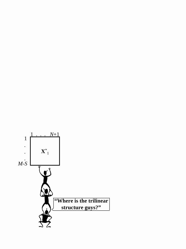
“Where is the trilinearstructure guys?”

X*1

1...

1 . . . N+1

M-S

Documents

Estimating Rate Constants of Chemical Reactions using ...three-mode.leidenuniv.nl/bibliogr/bijlsmas_thesis/thesisbijlsma.pdf · Estimating Rate Constants of Chemical Reactions using