remote sensing

Article

Estimation of the Motion-InducedHorizontal-Wind-Speed Standard Deviation in anOffshore Doppler Lidar

Miguel A. Gutiérrez-Antuñano 1 , Jordi Tiana-Alsina 2 , Andreu Salcedo 1 andFrancesc Rocadenbosch 1,3,*

1 CommSensLab, Unidad de Excelencia María de Maeztu, Department of Signal Theory and Communications,Universitat Politècnica de Catalunya (UPC), E-08034 Barcelona, Spain;miguel.angel.gutierrez@upc.edu (M.A.G.-A.); andreusalbos@gmail.com (A.S.)

2 Nonlinear Dynamics, Nonlinear Optics and Lasers (DONLL), Department of Physics (DFIS),Universitat Politècnica de Catalunya (UPC), E-08222 Terrassa, Spain; jordi.tiana@upc.edu

3 Institut d’Estudis Espacials de Catalunya (IEEC), Universitat Politècnica de Catalunya, E-08034 Barcelona,Spain

* Correspondence: roca@tsc.upc.edu

Received: 30 October 2018; Accepted: 11 December 2018; Published: 14 December 2018�����������������

Abstract: This work presents a new methodology to estimate the motion-induced standarddeviation and related turbulence intensity on the retrieved horizontal wind speed by means of thevelocity-azimuth-display algorithm applied to the conical scanning pattern of a floating Doppler lidar.The method considers a ZephIR™300 continuous-wave focusable Doppler lidar and does not requireaccess to individual line-of-sight radial-wind information along the scanning pattern. The methodcombines a software-based velocity-azimuth-display and motion simulator and a statistical recursiveprocedure to estimate the horizontal wind speed standard deviation—as a well as the turbulenceintensity—due to floating lidar buoy motion. The motion-induced error is estimated from thesimulator’s side by using basic motional parameters, namely, roll/pitch angular amplitude andperiod of the floating lidar buoy, as well as reference wind speed and direction measurements atthe study height. The impact of buoy motion on the retrieved wind speed and related standarddeviation is compared against a reference sonic anemometer and a reference fixed lidar over a 60-dayperiod at the IJmuiden test site (the Netherlands). Individual case examples and an analysis of theoverall campaign are presented. After the correction, the mean deviation in the horizontal windspeed standard deviation between the reference and the floating lidar was improved by about 70%,from 0.14 m/s (uncorrected) to −0.04 m/s (corrected), which makes evident the goodness of themethod. Equivalently, the error on the estimated turbulence intensity (3–20 m/s range) reduced from38% (uncorrected) to 4% (corrected).

Keywords: wind energy; remote sensing; Doppler wind lidar; velocity-azimuth-display algorithm;resource assessment; offshore; turbulence intensity

1. Introduction

In recent years, offshore wind energy has become a trustable and mature technology for electricitygeneration [1]. At the end of 2016, 14 GW cumulative offshore wind capacity proved the importance ofthis technology in the energy mix, with Europe being the main area of development but also with asignificant contribution from China [2]. Although most of the commercial developments of floatinglidars are being carried out in shallow waters (0–30 m), their benefits are not limited to these depths

Remote Sens. 2018, 10, 2037; doi:10.3390/rs10122037 www.mdpi.com/journal/remotesensing

Remote Sens. 2018, 10, 2037 2 of 19

and there is a tendency to go further off-coast to higher depths [3], where the advantages of floatinglidar technology versus conventional anemometry are more significant.

Different remote sensing technologies have been used in wind energy, including satellitemeasurements in offshore environments [4,5], radar [6], sodar [7–9], and combined techniques [10,11].Nevertheless, due to the high requirements of the industry regarding resolution and accuracy, lidar hasbeen the most used technology for different applications in the wind energy sector since the appearanceof the first commercial units. These applications include turbine control [12], resource assessment [13–15],wakes [16–18], and power curve measurements in flat terrain [19], among others.

In the resource assessment phase of offshore wind farms, floating lidars have become analternative to conventional fixed metmasts because lidar allows more flexibility in the deployment ina cost-effective way [13,20–23]. In 2015, the Carbon Trust published a roadmap for the commercialacceptance of this technology in the wind industry [24]. A state-of-the-art report and recommendedpractices developed by the IEA Wind Task 32 [25] can be found in [26], and several validation testsand commercial developments in [27–33].

The increasing use of floating lidar systems in the offshore wind energy sector motivates the needto assess and compensate the effect of motion on floating lidar measurements [34,35]. It has beenshown that both the static [36] and dynamic tilt [37–40] of the lidar instrument induce errors in theretrieved horizontal wind speed (HWS). Different approaches can be considered to reduce the impactof sea-waves-induced motion on the wind speed measured by floating lidar devices: mechanical [41,42]and numerical compensation methods [43,44].

Turbulence intensity (TI), which is defined as the ratio between the standard deviation of the HWSto the mean HWS, has a critical impact on wind turbine production, loads and design. The IEC61400-1Normal Turbulence Model describes the TI threshold a wind turbine is designed for, and defines thewind turbine class of the machine that describes the external conditions that must be considered [45–47].The lidar-observed TI is not identical to the “true” TI that can be measured by point-like measurementsfrom cup anemometers. The lidar-observed TI is affected by the spatial (i.e., probe length) andtemporal averaging (i.e., scanning time) of the Doppler lidar instrument and by the motion effectsof sea waves on the lidar buoy. While spatial/temporal averaging effects on the measured TI can befound elsewhere [48–51], here we aim at studying the effects of lidar motion on the measured TI and theirstatistical correction. To simplify the mathematical framework to be presented next, we numericallyassessed the motion-corrected HWS standard deviation under simple harmonic motion conditions ofthe lidar buoy for a given HWS and wind direction (WD). Towards this end, we considered a softwaremotion simulator to emulate the motion of sea waves under these simplified motion conditions and thevelocity-azimuth-display (VAD) algorithm [52] to retrieve the motion-corrupted HWS. Furthermore,simulation results were validated against experimental results as part of the IJmuiden test campaign.

This paper is organized as follows: Section 2 begins with a short description of the measurementinstrumentation at IJmuiden and follows with a description of the methods used: it revisits thevelocity-azimuth-display simulator, presents simulation examples of dynamic tilting of the lidar buoyunder different initial conditions, and describes the proposed methodology to compute the standarddeviation of the HWS error induced by lidar motion. Section 3 discusses the simulator’s resultsfrom the IJmuiden data. Three study cases for different sea and atmospheric conditions are analysed.The overall performance of the proposed methodology for the whole 60-day measurement campaignis also presented. Finally, Section 4 gives concluding remarks.

2. Materials and Methods

2.1. Materials

The ZephIR™300 lidar used in this work is a continuous-wave focusable Doppler lidaradapted for offshore measurements that uses a conical scanning pattern combined with thevelocity-azimuth-display algorithm to retrieve the wind velocity. The scan period is 1 s and each scan

Remote Sens. 2018, 10, 2037 3 of 19

is composed of 50 lines of sight. The lidar can retrieve the wind vector between 10 and 200 m in heightin user-defined steps of 1 m, although not simultaneously. The latter is a consequence of the focusingprinciple of the instrument, which also yields a height-dependent spatial resolution (e.g., 15 m at 100 min height).

As described in [53], a validation campaign of the floating lidar was performed at the IJmuidentest site [54,55]. The aim of this campaign was to assess the accuracy of the EOLOS lidar buoy againstmetmast IJmuiden [24]. The main instruments used were: (i) a moving ZephIR™300 lidar in a buoy,measuring at 27, 58, and 85 m above the Lowest Astronomical Tide (LAT); (ii) a reference ZephIR™300lidar placed on the metmast platform and measuring at 90, 115, 140, 165, 190, 215, 240, 265, 290, and315 m above LAT, both measuring sequentially at each height; and (iii) sonic anemometers at 27, 58,and 85 m above LAT. The ZephIR™300 lidar has shown to be a reliable device for on- and offshorewind-energy applications. More detailed information about these sensors and additional sensorsin the metmast can be found in [54]. Additionally, data from inertial measurement units were usedto characterise the motion of the lidar buoy. In the present work, data from 1 April to 1 June 2015were used.

2.2. The Velocity–Azimuth-Display Motion Simulator

The velocity-azimuth-display (VAD) algorithm enables the retrieval of the three components ofthe wind-speed vector from a vertically-pointing, conically-scanning Doppler lidar, as is the case ofthe ZephIR™300. Under the assumption of a constant wind vector, it can be shown that the radialwind speed component along the lidar line of sight as a function of the scan time follows a sinusoidalpattern (the so-called VAD pattern). The wind speed components can be retrieved from the amplitudeand offset and this sinusoidal pattern by using geometrical considerations and a simple least-squaresfitting procedure [52,56].

In previous works [40], we have presented the formulation of the VAD motion simulator underthe assumption of a time-invariant and horizontally-homogeneous wind field. The simulator usesEuler’s angles to compute the rotated line-of-sight vector at a given time in response to simultaneouspitch, roll, and yaw tilting angles (three degrees of freedom). Because the rotation matrix of the buoycan numerically be computed as a function of discrete time in response to harmonic excitations in thesethree angles, it is possible to compute the rotated set of lines of sight of the lidar for each conical scanin response to buoy motion. When the VAD retrieval algorithm is applied to the radial wind speedonto the rotated set of lines of sight, the motion-induced HWS is retrieved with a temporal resolutionof 1 s (scan period of the ZephIR™300). In principle, the simulation process is complicated by theexistence of three degrees of freedom, each one being described by three variables (i.e., amplitude,phase, and frequency) representing the sinusoidal excitation. In practice, dependence on the yaw isnot considered because yaw motion can be considered static as compared to the lidar scan period.Therefore, wind direction errors caused by yaw motion are corrected by means of the buoy compass.The fact that the scan phase of the lidar scanning pattern (i.e., the starting line of sight of the scanningpattern at time zero) is completely uncorrelated with buoy roll/pitch movement forced us to carry outthe study by defining different constraints on these variables (this is further discussed in Sections 2.3and 2.4). Thus, two simple cases were considered in the publication above: static and dynamic buoytilting. The latter was limited to specific constraints: (i) only one degree-of-freedom (either roll or pitch);(ii) zero initial phase of the angular movement; and (iii) zero scan phase of the VAD scanning pattern.

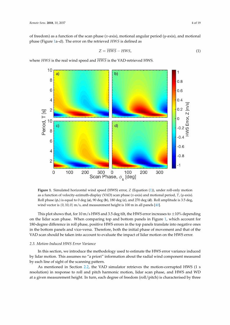
In the present paper, we overcome these constraints by considering: (i) the combined contributionsfrom both roll and pitch degrees of freedom; (ii) all possible phases in roll and pitch motion; and (iii) allpossible phases in the VAD scan. To illustrate the importance of these parameters, Figure 1 plots thesimulated error on the VAD-retrieved HWS (Equation (1) next) under roll-only lidar motion (one degree

Remote Sens. 2018, 10, 2037 4 of 19

of freedom) as a function of the scan phase (x-axis), motional angular period (y-axis), and motionalphase (Figure 1a–d). The error on the retrieved HWS is defined as

Z = HWS− HWS, (1)

where HWS is the real wind speed and HWS is the VAD-retrieved HWS.

Figure 1. Simulated horizontal wind speed (HWS) error, Z (Equation (1)), under roll-only motionas a function of velocity-azimuth-display (VAD) scan phase (x-axis) and motional period, T, (y-axis).Roll phase (φr) is equal to 0 deg (a), 90 deg (b), 180 deg (c), and 270 deg (d). Roll amplitude is 3.5 deg,wind vector is (0, 10, 0) m/s, and measurement height is 100 m in all panels [40].

This plot shows that, for 10 m/s HWS and 3.5 deg tilt, the HWS error increases to±10% dependingon the lidar scan phase. When comparing top and bottom panels in Figure 1, which account for180-degree difference in roll phase, positive HWS errors in the top panels translate into negative onesin the bottom panels and vice-versa. Therefore, both the initial phase of movement and that of theVAD scan should be taken into account to evaluate the impact of lidar motion on the HWS error.

2.3. Motion-Induced HWS Error Variance

In this section, we introduce the methodology used to estimate the HWS error variance inducedby lidar motion. This assumes no “a priori” information about the radial wind component measuredby each line of sight of the scanning pattern.

As mentioned in Section 2.2, the VAD simulator retrieves the motion-corrupted HWS (1 sresolution) in response to roll and pitch harmonic motion, lidar scan phase, and HWS and WDat a given measurement height. In turn, each degree of freedom (roll/pitch) is characterised by three

Remote Sens. 2018, 10, 2037 5 of 19

variables—namely, amplitude, period, and phase. Therefore, the HWS retrieved by the VAD motionsimulator can be expressed as

HWS = h(HWS, WD, H, Ar, φr, Tr, Ap, φp, Tp, φs), (2)

where h is the nonlinear function modelling the VAD-fitting algorithm, H is the measurementheight, and A, φ, and T are the amplitude, phase, and period associated to sinusoidal roll/pitchmotional excitation, A · sin(2π f t + φ), with f = 1

T (subscripts r and p stand for roll and pitch angles,respectively), and φs is the conical scan phase of the lidar.

Horizontal wind speed (HWS), wind direction (WD), and roll/pitch amplitudes and periods(Ar/p, Tr/p, respectively) are deterministic variables because they can be measured experimentally(e.g., HWS and WD from metmast anemometers or a reference fixed lidar, and roll/pitch amplitudesand periods from inertial measurement units on the buoy). In contrast, roll/pitch motional phases,φr/p, and VAD scan phase, φs, become random variables because buoy initial motion conditions (φr/p)cannot be recovered from inertial measurement unit measurements, nor is the scan phase (φs) availablefrom the lidar.

For convenience, we define HWS-error function g as Equation (2) above, constrained to the setof deterministic conditions ~S = (HWS, WD, Ap, Tp, Ar, Tr) (i.e., given HWS, WD, and buoy attitude)minus the true HWS,

Z = g(φr, φp, φs) = h|~S − HWS. (3)

The motion-induced HWS error variance can be estimated for the first and second raw momentsof Z as

Var(Z) = E(Z2)− E(Z)2. (4)

By using the expectation theorem [57], the first two raw moments of Z can be computed as

E(Zn) =∫ ∞

−∞

∫ ∞

−∞

∫ ∞

−∞g(φr, φp, φs)

n fΦrΦpΦs(φr, φp, φs)dφrdφpdφs, (5)

where fΦrΦpΦs(φr, φp, φs) is the joint probability distribution function for the random-variable set ofphases, Φr, Φp, and Φs; and n = 1, 2. At this point, and following standard notation in probabilitytheory [58], we use uppercase Greek letters to denote random variables and lowercase letters to denotethe values for these variables.

Formulation of the multivariate distribution function fΦrΦpΦs(φr, φp, φs) can largely be simplifiedby introducing different properties describing the statistics of random variables Φr, Φp and Φs.We hypothesise that information about any one of these three variables gives no information about theother two, which is equivalent to saying that phases Φr, Φp and Φs are independent random variables.This will be further discussed in Section 2.4. As a result, joint density function fΦrΦpΦs factors outas the product of univariate functions fΦr , fΦp and fΦs , as fΦrΦpΦs = fΦr fΦp fΦs . This enables us torewrite Equation (5) as

E(Zn) =∫ 2π

0

∫ 2π

0fΦr (φr) fΦp(φp)

[ ∫ 2π

0g(φr, φp, φs)

n fΦs(φs)dφs

]dφrdφp, (6)

where it has been used that random variables Φr, Φp, and Φs are uniformly distributed in [0, 2π) so that

fν(ν) =1

2π, ν ∈ [0, 2π) with ν = φr, φp, φs. (7)

The hypothesis of uniform distribution in [0, 2π) for scan phase Φs is well-justified on account ofthe fact that, despite the 1 s temporal resolution of the lidar, measurements are not exactly deliveredevery second due to lidar refocusing and internal checkings.

Remote Sens. 2018, 10, 2037 6 of 19

We define

g′n(φr, φp) =∫ 2π

0g(φs)

n∣∣∣∣Φr=φr ,Φp=φp

fΦs(φs)dφs, (8)

which can physically be understood as the n-th raw moment of the HWS error due to random variablescan phase, Φs, for a given pair of roll and pitch phases, Φr = φr and Φp = φp. Equivalently,Equation (8) can be written as

g′n(φr, φp) = E(g(φs)n∣∣∣∣Φr=φr ,Φp=φp

, (9)

which is the expected value of g(φs)n for a particular pair of motional phases Φr = φr and Φp = φp.Because fΦs is a uniform probability density function, the expected value is just the arithmetic mean ofg(φs)n along the Φs dimension.

By substituting Equation (8) into Equation (6), Equation (6) takes the form

E(Zn) =∫ 2π

0fΦr (φr)

[ ∫ 2π

0g′n(φr, φp) fΦp(φp)dφp

]dφr. (10)

By comparing Equation (10) to Equation (6) above, it emerges that we reduced the calculus fromthe tri-dimensional domain [Φr, Φp, Φs] in Equation (6) to the bi-dimensional domain [Φr, Φp] inEquation (10). The same procedure above can be repeated recursively to reduce Equation (10) fromthe bi-dimensional domain [Φr, Φp] to the one-dimensional domain, [Φr]. Thus, in similar fashion toEquation (8), we define

g′′n(φr) =∫ 2π

0g′n(φp)

∣∣∣∣Φr=φr

fΦp(φp)dφp, (11)

which can also be written as (counterpart of Equation (9))

g′′n(φr) = E(g′n(φp)

∣∣∣∣Φr=φr

. (12)

Substitution of Equation (11) into Equation (6) yields

E(Zn) =∫ 2π

0g′′n(φr) fΦr (φr)dφr, (13)

or, equivalently,E(Zn) = E(g′′n(φr)), (14)

which is to say that the raw moments of the HWS error function Z can be calculated by using athree-step procedure given by Equations (9), (12) and (14), where the contribution from each randomvariable (i.e., roll phase, Φr, pitch phase, Φp, and scan phase, Φs) are successively averaged out.

The practical computational procedure of Equations (9), (12) and (14) is as follows: for a given setof simulation parameters ~S = (HWS, WD, H, Ap, Tp, Ar, Tr), the HWS error (Equation (1)) is calculatedby the motion simulator of Section 2.2 in the [0− 2π)× [0− 2π)× [0− 2π) domain of random phasesΦr, Φp, and Φs by using a grid of 24× 24× 24 evenly spaced points between 0 and 2π. This gives a 3Dmatrix of HWS error values similar to the 2D matrix represented in Figure 1, but in three dimensions.Then, the HWS error is averaged along the Φs (scan phase) dimension of the matrix for every pairof roll/pitch phase values (φr, φp) to obtain g′1 (1st raw moment, Equation (9)). Next, this procedureis repeated recursively over the Φp dimension of g′1 (now a 2D instead of a 3D matrix) to yield g′′1 (a1D matrix or vector, Equation (12)), and finally, over the Φr dimension of g′′1 , which yields the scalarE(Z) (Equation (6)). This three-step procedure is repeated twice to compute E(Z) and E(Z2). Finally,

Remote Sens. 2018, 10, 2037 7 of 19

the sought-after HWS error variance, Var(Z), is obtained from Equation (4). The standard deviation ofthe motion-induced HWS error, σZ, is computed as the square root of the variance.

2.4. Roll/Pitch Correlation Hypothesis

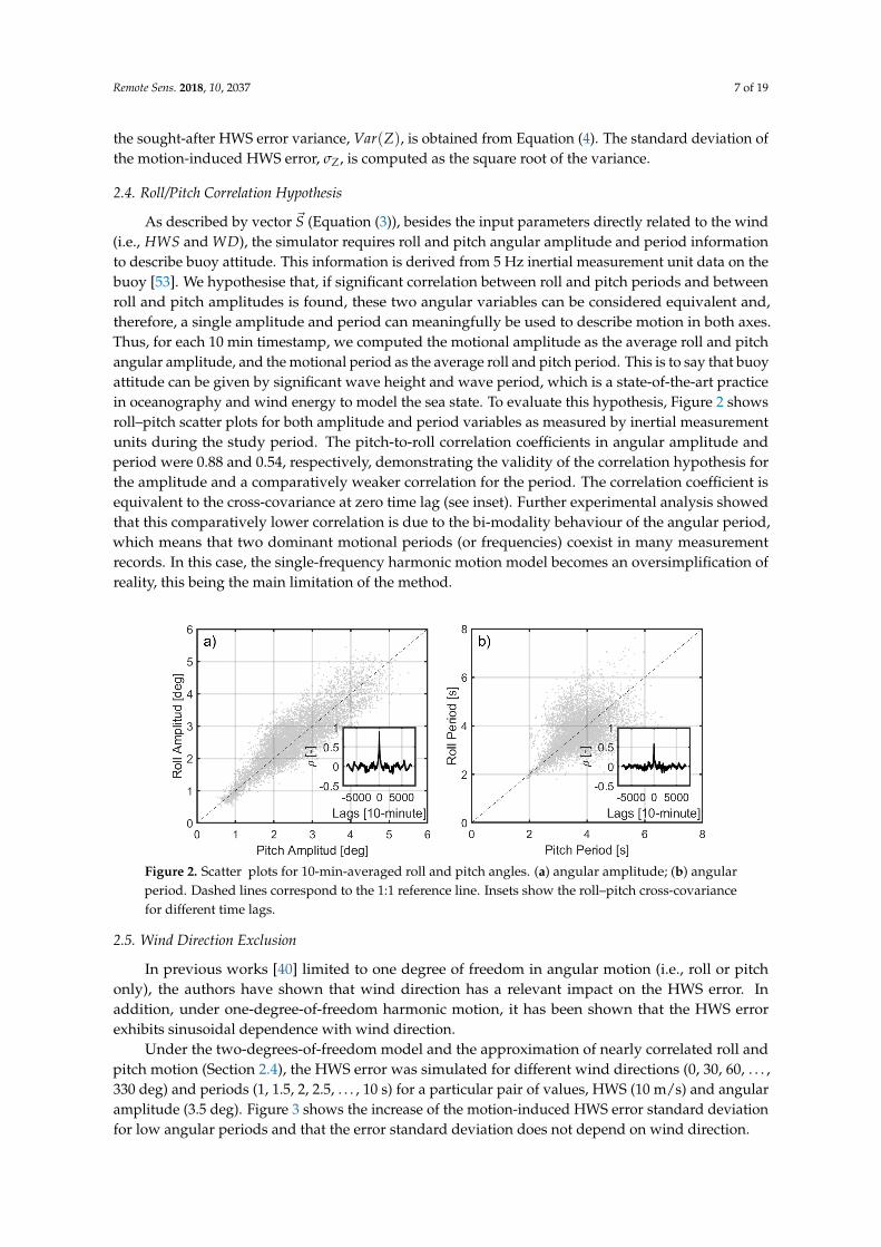
As described by vector ~S (Equation (3)), besides the input parameters directly related to the wind(i.e., HWS and WD), the simulator requires roll and pitch angular amplitude and period informationto describe buoy attitude. This information is derived from 5 Hz inertial measurement unit data on thebuoy [53]. We hypothesise that, if significant correlation between roll and pitch periods and betweenroll and pitch amplitudes is found, these two angular variables can be considered equivalent and,therefore, a single amplitude and period can meaningfully be used to describe motion in both axes.Thus, for each 10 min timestamp, we computed the motional amplitude as the average roll and pitchangular amplitude, and the motional period as the average roll and pitch period. This is to say that buoyattitude can be given by significant wave height and wave period, which is a state-of-the-art practicein oceanography and wind energy to model the sea state. To evaluate this hypothesis, Figure 2 showsroll–pitch scatter plots for both amplitude and period variables as measured by inertial measurementunits during the study period. The pitch-to-roll correlation coefficients in angular amplitude andperiod were 0.88 and 0.54, respectively, demonstrating the validity of the correlation hypothesis forthe amplitude and a comparatively weaker correlation for the period. The correlation coefficient isequivalent to the cross-covariance at zero time lag (see inset). Further experimental analysis showedthat this comparatively lower correlation is due to the bi-modality behaviour of the angular period,which means that two dominant motional periods (or frequencies) coexist in many measurementrecords. In this case, the single-frequency harmonic motion model becomes an oversimplification ofreality, this being the main limitation of the method.

Figure 2. Scatter plots for 10-min-averaged roll and pitch angles. (a) angular amplitude; (b) angularperiod. Dashed lines correspond to the 1:1 reference line. Insets show the roll–pitch cross-covariancefor different time lags.

2.5. Wind Direction Exclusion

In previous works [40] limited to one degree of freedom in angular motion (i.e., roll or pitchonly), the authors have shown that wind direction has a relevant impact on the HWS error. Inaddition, under one-degree-of-freedom harmonic motion, it has been shown that the HWS errorexhibits sinusoidal dependence with wind direction.

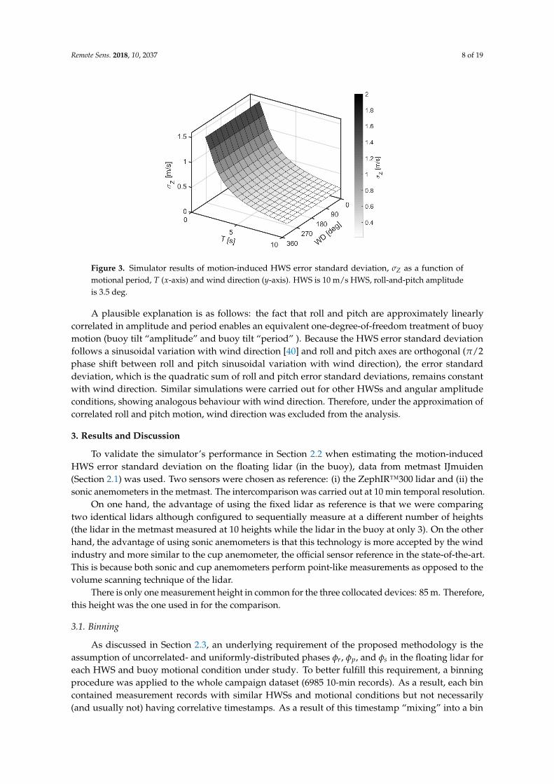
Under the two-degrees-of-freedom model and the approximation of nearly correlated roll andpitch motion (Section 2.4), the HWS error was simulated for different wind directions (0, 30, 60, . . . ,330 deg) and periods (1, 1.5, 2, 2.5, . . . , 10 s) for a particular pair of values, HWS (10 m/s) and angularamplitude (3.5 deg). Figure 3 shows the increase of the motion-induced HWS error standard deviationfor low angular periods and that the error standard deviation does not depend on wind direction.

Remote Sens. 2018, 10, 2037 8 of 19

Figure 3. Simulator results of motion-induced HWS error standard deviation, σZ as a function ofmotional period, T (x-axis) and wind direction (y-axis). HWS is 10 m/s HWS, roll-and-pitch amplitudeis 3.5 deg.

A plausible explanation is as follows: the fact that roll and pitch are approximately linearlycorrelated in amplitude and period enables an equivalent one-degree-of-freedom treatment of buoymotion (buoy tilt “amplitude” and buoy tilt “period” ). Because the HWS error standard deviationfollows a sinusoidal variation with wind direction [40] and roll and pitch axes are orthogonal (π/2phase shift between roll and pitch sinusoidal variation with wind direction), the error standarddeviation, which is the quadratic sum of roll and pitch error standard deviations, remains constantwith wind direction. Similar simulations were carried out for other HWSs and angular amplitudeconditions, showing analogous behaviour with wind direction. Therefore, under the approximation ofcorrelated roll and pitch motion, wind direction was excluded from the analysis.

3. Results and Discussion

To validate the simulator’s performance in Section 2.2 when estimating the motion-inducedHWS error standard deviation on the floating lidar (in the buoy), data from metmast IJmuiden(Section 2.1) was used. Two sensors were chosen as reference: (i) the ZephIR™300 lidar and (ii) thesonic anemometers in the metmast. The intercomparison was carried out at 10 min temporal resolution.

On one hand, the advantage of using the fixed lidar as reference is that we were comparingtwo identical lidars although configured to sequentially measure at a different number of heights(the lidar in the metmast measured at 10 heights while the lidar in the buoy at only 3). On the otherhand, the advantage of using sonic anemometers is that this technology is more accepted by the windindustry and more similar to the cup anemometer, the official sensor reference in the state-of-the-art.This is because both sonic and cup anemometers perform point-like measurements as opposed to thevolume scanning technique of the lidar.

There is only one measurement height in common for the three collocated devices: 85 m. Therefore,this height was the one used in for the comparison.

3.1. Binning

As discussed in Section 2.3, an underlying requirement of the proposed methodology is theassumption of uncorrelated- and uniformly-distributed phases φr, φp, and φs in the floating lidar foreach HWS and buoy motional condition under study. To better fulfill this requirement, a binningprocedure was applied to the whole campaign dataset (6985 10-min records). As a result, each bincontained measurement records with similar HWSs and motional conditions but not necessarily(and usually not) having correlative timestamps. As a result of this timestamp “mixing” into a bin

Remote Sens. 2018, 10, 2037 9 of 19

(also called time “scrambling”), the requirement of uncorrelated and uniformly distributed phases(Section 2.3) into a bin was reinforced. The chosen binning variables were: HWS, angular amplitude,and period in equally spaced bins of width 1 unit ((m/s), (deg), and (s), respectively) centred on integervalues (bin edges at [0.5 1.5), [1.5 2.5) units, etc.).

Table 1 shows the 25 most frequent cases in the IJmuiden campaign. The most common HWSs werebetween 3 and 12 m/s, amplitudes were between 2 and 4 degrees, and motional periods were between3 and 4 s. The total set of measurement cases is considered in Figure 6 and Section 3.4. The conditionsof the site during the study period included HWS between 2 and 21 m/s, angular amplitudes between1 and 5 deg, and periods between 2 and 5 s.

Table 1. The 25 most frequent HWS and motional cases in the IJmuiden campaign. “Case no.” is thebin number sorted by decreasing frequency of event occurrence (“1” indicating the most frequentcase); HWS (m/s) stands for 10-min mean horizontal wind speed; AA (deg) stands for motionangular amplitude; T (s) stands for period; Count no. is the bin count number; and σZ (m/s) isthe motion-induced HWS error standard deviation estimated by the simulator after Equation (4).

Case No. HWS (m/s) AA (deg) T (s) Count No. σZ (m/s)

1 8 3 4 288 0.182 5 2 4 247 0.073 9 3 4 237 0.204 7 2 4 208 0.105 6 2 4 198 0.096 7 3 4 196 0.167 6 3 4 182 0.138 6 2 3 180 0.129 3 2 4 175 0.0410 7 2 3 174 0.1411 10 3 4 169 0.2212 5 2 3 166 0.1013 4 2 4 164 0.0614 8 2 4 157 0.1215 8 2 3 133 0.1616 11 3 4 130 0.2517 5 3 4 130 0.1118 9 3 3 112 0.2719 8 3 3 108 0.2420 7 3 3 106 0.2121 12 3 4 100 0.2722 11 4 4 95 0.3323 2 1 3 91 0.0224 4 2 3 86 0.0825 3 1 3 80 0.03

3.2. Variance of the Sum of Partially Correlated Variables

Next, we discuss how to combine the motion-induced HWS error standard deviation, σZ,estimated by the simulator (Section 2.3), with the reference HWS standard deviation, σre f , which ismeasured from either the lidar on the metmast, σre f (lidar), or the sonic anemometer, σre f (sonic), in orderto estimate the motion-corrected HWS standard deviation, σcorr. The latter is the key output of our studyto be compared with the HWS standard deviation measured by the floating lidar, σmoving.

According to the law of propagation of errors, the corrected variance, σ2corr, of the sum of two

variables (the real wind speed (or reference), HWS, and the motion-induced HWS error, Z; Equation (1))is written as [57]

σ2corr = σ2

re f + σ2Z + 2 cov(re f , Z), (15)

Remote Sens. 2018, 10, 2037 10 of 19

where σ2 stands for variance (i.e., the square of the standard deviation) and cov(re f , Z) is the covariancebetween the reference HWS and the motion-induced HWS error.

Equation (15) above states that the standard deviation of the HWS measured by the moving lidarnot only depends on the variance from both the wind (intrinsic turbulence) and the motion-inducederror, but also on the covariance between these two variables. In the limit cases of: (i) uncorrelatedvariables (U), cov(re f , Z) = 0, and (ii) linearly correlated variables (C), cov(re f , Z) = σre f · σZ,Equation (15) reduces to

σUcorr =

√σ2

re f + σ2Z, (16)

σCcorr = σre f + σZ. (17)

In what follows, and unless otherwise stated, the motion-corrected HWS standard deviation σcorr iscalculated assuming partial correlation between these variables (i.e., by using Equation (15)). The termcov(re f , Z) is computed from the correlation coefficient between the reference HWS, re f , and theexpected value of the motion-induced HWS error, E(Z). Here, we use the mathematical definitioncov(re f , Z) = ρre f ,Z · σre f · σZ, where ρre f ,Z is the correlation coefficient, and σre f and σZ are thestandard deviations of the 10-min reference HWS and 10-min motion-induced HWS error, respectively.In practice, and considering that the binning process ensures similar motional characteristics in eachbin (Section 3.1), we computed a single ordered pair (reference HWS, E(Z)) per bin (109 simulations)and a single correlation coefficient given these 109 bins (ρ = 0.78), which is representative of themotional conditions of the overall sample under study.

3.3. Analysis of Particular Cases

In order to discuss the goodness of the proposed methodology to estimate the motion-inducedHWS standard deviation, this section tackles three representative cases (or bins) from Table 1: casesno. 2, 18, and 25. The first case gave good estimation of the motion-induced HWS standard deviation;the second one, overestimation; and the third one, underestimation.

Figure 4 plots the standard deviation of the HWS with and without correction (Equation (15)),using the lidar on the metmast as reference. The sample size associated with each of these three casesis listed in the “Count no.” column of Table 1.

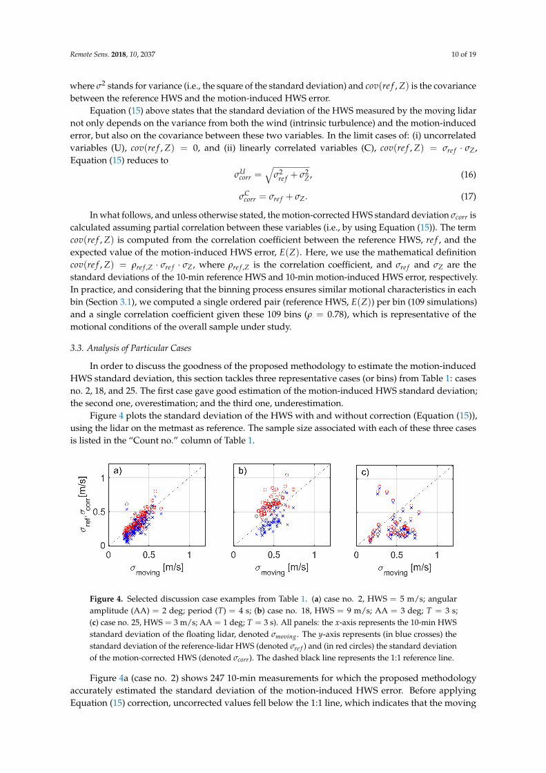
Figure 4. Selected discussion case examples from Table 1. (a) case no. 2, HWS = 5 m/s; angularamplitude (AA) = 2 deg; period (T) = 4 s; (b) case no. 18, HWS = 9 m/s; AA = 3 deg; T = 3 s;(c) case no. 25, HWS = 3 m/s; AA = 1 deg; T = 3 s). All panels: the x-axis represents the 10-min HWSstandard deviation of the floating lidar, denoted σmoving. The y-axis represents (in blue crosses) thestandard deviation of the reference-lidar HWS (denoted σre f ) and (in red circles) the standard deviationof the motion-corrected HWS (denoted σcorr). The dashed black line represents the 1:1 reference line.

Figure 4a (case no. 2) shows 247 10-min measurements for which the proposed methodologyaccurately estimated the standard deviation of the motion-induced HWS error. Before applyingEquation (15) correction, uncorrected values fell below the 1:1 line, which indicates that the moving

Remote Sens. 2018, 10, 2037 11 of 19

lidar “saw” a higher standard deviation. After Equation (15) correction, most of the measurementslaid on the 1:1 reference line.

Figure 4b,c, which are representative of case nos. 18 and 25, respectively, show two oppositesituations: on one hand, for case no. 18 (Figure 4b), the simulator overestimated the influence of motionand the corrected values laid above the 1:1 line. Further investigation showed that this can be caused bythe lack of consistency of the roll/pitch correlation hypothesis (Section 2.4) due to most measurementsundergoing bi-modal motion behaviour. On the other hand, case no. 25 (Figure 4c) showed correctedvalues falling nearly always below the 1:1 line, which means that the estimated correction givenby the motion simulator was too low. Further inspection indicated that this underestimation wascaused by untrustworthy retrieval of the HWS by the VAD algorithm, as made evident by too-highspatial variation (SV) values from the ZephIR™300 lidar (Figure 5, to be discussed in Section 3.4). Thespatial variation is a lidar internal parameter related to the goodness of fit that reveals whether themeasurement data is consistent or not with the sinusoidal model assumed by the VAD algorithm.Thus, high SV values are related to a poor VAD fitting, and they are usually found in low HWS, whereTaylor’s frozen-eddies hypothesis is no longer true and the lidar does not measure a homogeneouswind along the VAD scanning area.

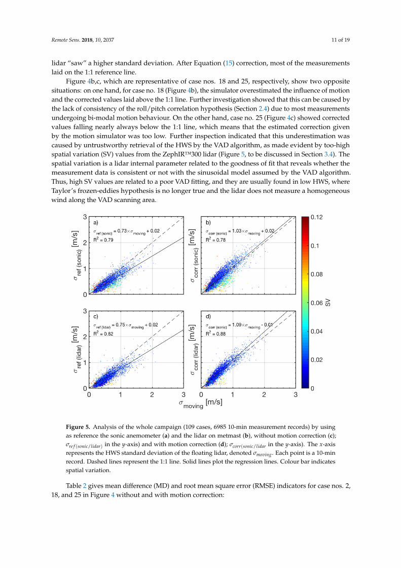
Figure 5. Analysis of the whole campaign (109 cases, 6985 10-min measurement records) by usingas reference the sonic anemometer (a) and the lidar on metmast (b), without motion correction (c);σre f (sonic/lidar) in the y-axis) and with motion correction (d); σcorr(sonic/lidar in the y-axis). The x-axisrepresents the HWS standard deviation of the floating lidar, denoted σmoving. Each point is a 10-minrecord. Dashed lines represent the 1:1 line. Solid lines plot the regression lines. Colour bar indicatesspatial variation.

Table 2 gives mean difference (MD) and root mean square error (RMSE) indicators for case nos. 2,18, and 25 in Figure 4 without and with motion correction:

Remote Sens. 2018, 10, 2037 12 of 19

Table 2. Statistical indicators with and without motion correction for the selected discussion caseexamples from Table 1. MD stands for mean deviation and RMSE stands for root mean square error(see text and Equations (18) and (19)). MD and RMSE units are (m/s).

Case No. Count No.

Reference Sonic Reference Lidar

Corrected Uncorrected Corrected Uncorrected

MD RMSE MD RMSE MD RMSE MD RMSE

2 247 0.08 0.15 0.14 0.19 0.02 0.08 0.08 0.1118 112 −0.10 0.18 0.14 0.21 −0.12 0.15 0.12 0.1525 80 0.20 0.26 0.22 0.28 0.20 0.31 0.22 0.33

The motion-corrected mean deviation is defined as

MDcorr =

∑i(σmoving,i − σcorr(x),i)

N, (18)

where N is the case “count no.” (Table 1), σmoving is the HWS standard deviation measured by thefloating lidar (already introduced in Section 3.2), and σcorr(x) is the motion-corrected HWS standarddeviation (Equation (15)) of the reference instrument, where x = lidar denotes the reference fixed lidarand x = sonic denotes the sonic anemometer. Subscript i is the count-number index, that is, i wentfrom i = 1 to i = 247 for case no. 2.

The motion-corrected root mean-square error is defined as

RMSEcorr =

√√√√∑i(σmoving,i − σcorr(x),i)

2

N. (19)

Similarly, uncorrected MD and RMSE indicators are computed by substituting σcorr(x),i withσre f (x),i, the reference HWS standard deviation, in Equations (18) and (19) above. These indicators aredenoted MDre f and RMSEre f , respectively.

The mean deviation gives an estimation of the systematic error, equivalently, the amount of bias,while the RMSE is the quadratic mean of differences, with an ideal value of 0 indicating a perfect fit.

As shown in Table 2, the mean deviation for case no. 2 improved from 0.08 (uncorrected) to0.02 m/s after motion correction. The RMSE also improved from 0.11 to 0.08 m/s. For overestimationcase no. 18, the mean deviation changed sign from 0.12 to −0.12 m/s and, for underestimation caseno. 25, the mean deviation virtually did not change (from 0.22 to 0.20 m/s). In over/underestimatedcase nos. 18 and 25, the RMSE did not improve after motion correction by Equation (15). All thingsconsidered, these indicators were consistent with the discussion carried out for Figure 4a–c, and theywere therefore used to quantitatively analyse the overall campaign in the following.

3.4. Analysis of the Whole Campaign

In this section, we discuss overall performance of the motion-corrected HWS standard deviation,σcorr, calculated via Equation (15) and, for comparison, via Equations (16) and (17), for the wholemeasurement campaign at IJmuiden (6985 10-min records clustered into 109 cases).

In similar fashion to Figure 4 but for the whole campaign, Figure 5 compares the HWS standarddeviation of the moving lidar, σmoving, to the motion-corrected standard deviation (Equation (15)) ofthe sonic and fixed-lidar reference devices (σcorr(sonic) and σcorr(lidar), respectively; right panels) andto the uncorrected ones (left panels; labelled σre f (sonic) and σre f (lidar)), respectively). Linear regressionparameters and correlation coefficients, superimposed on Figure 5, clearly improved after applying thecorrection methodology for both the sonic and the fixed-lidar references. Therefore, better agreementbetween the floating lidar and the instrumental references was obtained. Despite the improvement,

Remote Sens. 2018, 10, 2037 13 of 19

there was a tendency to slightly overestimate the motion-corrected standard deviation, σcorr,(x), x =

sonic, lidar, for both the sonic and lidar references.To further investigate this issue, each point in the scatter plots was colour-coded according to the

spatial variation given by the floating lidar. Blue dots, which are associated to low spatial variation,exhibited good correlation while poorly correlated points were associated to spatial-variation figuresabove 0.06. These high figures were usually due to errors in the VAD-retrieved HWS caused byinhomogeneity of the wind. This means that regression-line results could better approach the ideal1:1 line by filtering out these outliers on a spatial variation criterion, which is out of the scope of thepresent work.

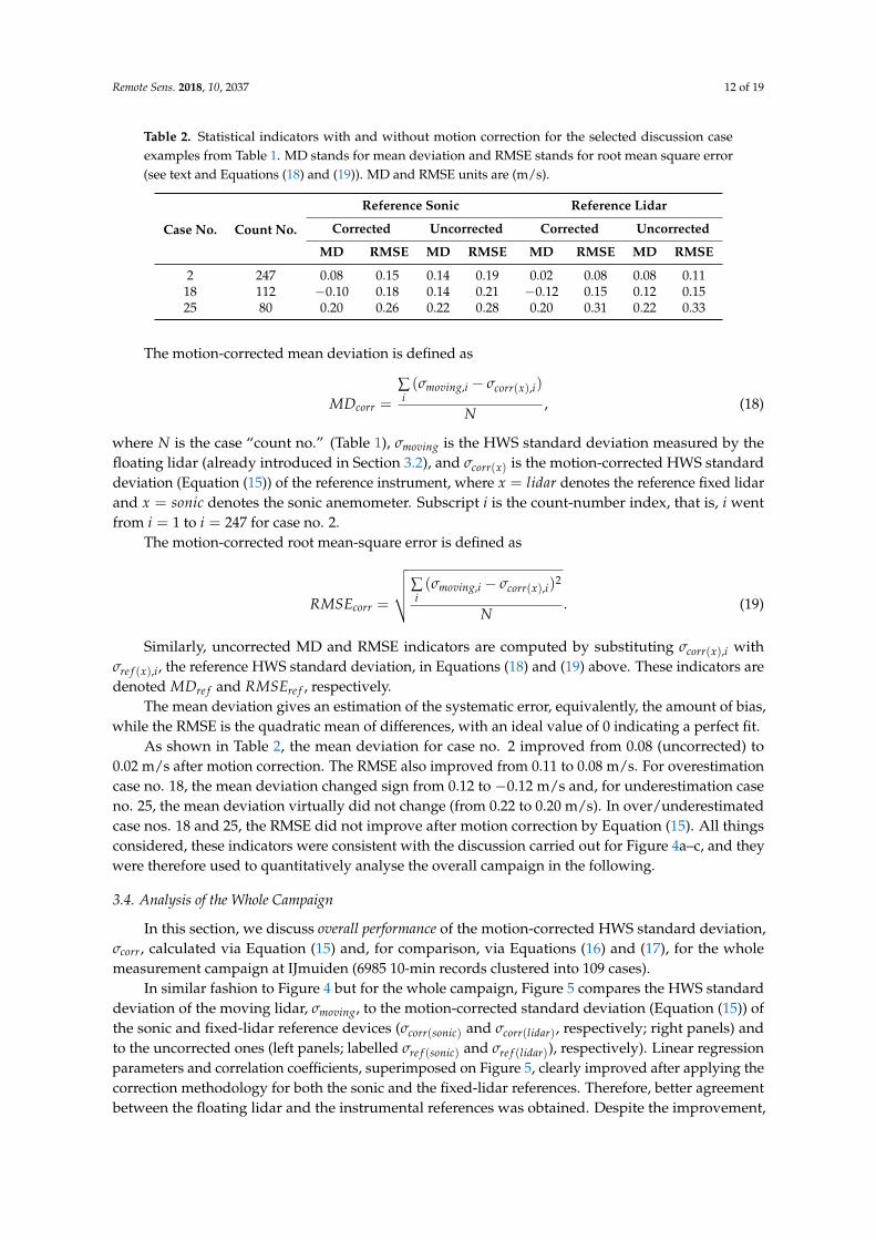
To quantitatively discuss the whole campaign via mean difference and root mean square errorindicators (Equations (18) and (19), Table 3 presents the results for all 109 cases in the campaign,for both the fixed lidar and sonic references. Results are graphically depicted in the histogram ofFigure 6 for the lidar reference only. Figure 6 shows that the motion-uncorrected mean difference,MDre f , had a positive bias of 0.13 m/s when using the fixed lidar as reference. This bias accountsfor the systematic error in the measured HWS standard deviation caused by floating lidar motionas previously reported in [27,59]. After motion correction, the mean difference MDcorr reduced tothe virtually unbiased figure of −0.03 m/s when using the fixed lidar as reference. The negativesign indicates the tendency to overestimate, as mentioned previously. This accounts for an 80%reduction in absolute value. Using the sonic anemometer as reference, the MD reduced from 0.12to −0.03 m/s (histogram not shown). The RMSE reduced from RMSEre f = 0.17 (uncorrected) toRMSEcorr = 0.12 m/s (motion corrected) when using the lidar reference (this accounts for a 29%reduction) and from 0.18 to 0.16 m/s when using the sonic reference. This is considered evidence ofthe accuracy of the proposed methodology in estimating the motion-induced standard deviation.

Table 3. Performance of the variance-combination laws of Section 3.2. (C) stands for linearly correlatedvariables, (PC) for partially correlated, and (U) for uncorrelated.

Variance-Combination Law for σcorrUncorrected, σre f

(C) Equation (17) (PC) Equation (15) (U) Equation (16)

Sonic Lidar Sonic Lidar Sonic Lidar Sonic Lidar

MD −0.06 −0.05 −0.03 −0.03 0.08 0.08 0.12 0.13RMSE 0.17 0.13 0.16 0.12 0.15 0.13 0.18 0.17

Figure 6. Histogram of the main statistical parameters. (a) mean difference; (b) root mean square errorusing the fixed lidar as reference; for all panels: blue = motion corrected, red = uncorrected.

Remote Sens. 2018, 10, 2037 14 of 19

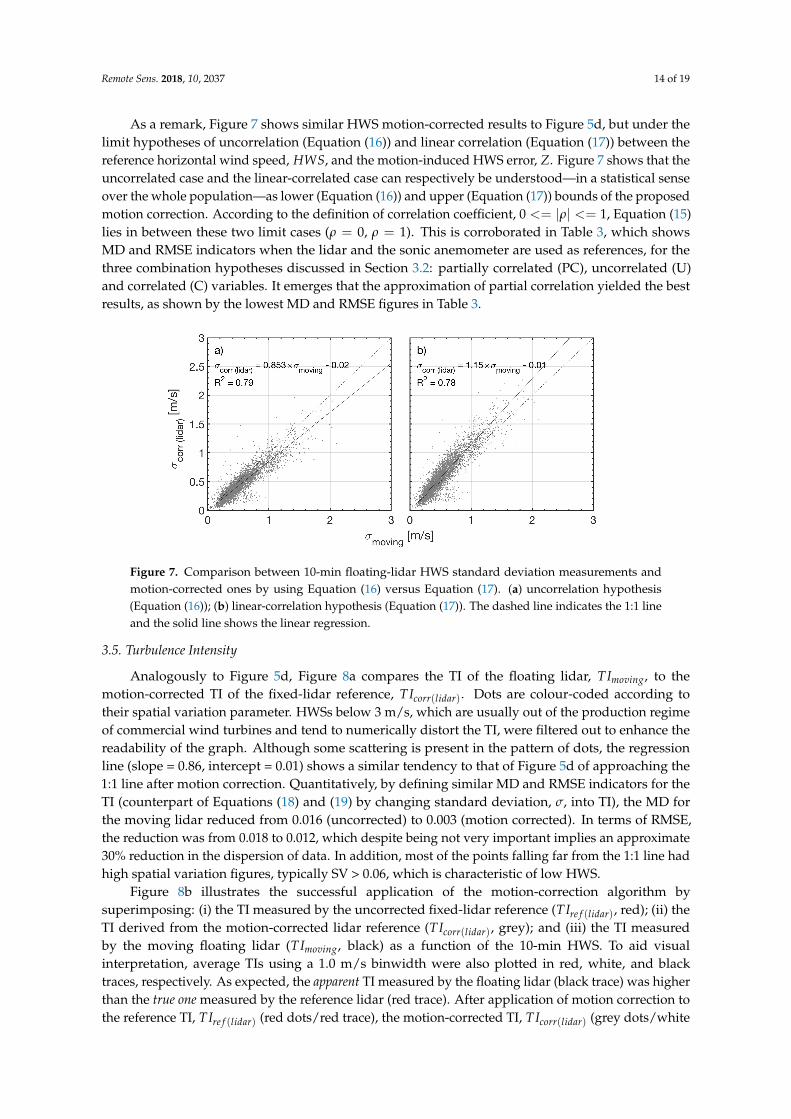
As a remark, Figure 7 shows similar HWS motion-corrected results to Figure 5d, but under thelimit hypotheses of uncorrelation (Equation (16)) and linear correlation (Equation (17)) between thereference horizontal wind speed, HWS, and the motion-induced HWS error, Z. Figure 7 shows that theuncorrelated case and the linear-correlated case can respectively be understood—in a statistical senseover the whole population—as lower (Equation (16)) and upper (Equation (17)) bounds of the proposedmotion correction. According to the definition of correlation coefficient, 0 <= |ρ| <= 1, Equation (15)lies in between these two limit cases (ρ = 0, ρ = 1). This is corroborated in Table 3, which showsMD and RMSE indicators when the lidar and the sonic anemometer are used as references, for thethree combination hypotheses discussed in Section 3.2: partially correlated (PC), uncorrelated (U)and correlated (C) variables. It emerges that the approximation of partial correlation yielded the bestresults, as shown by the lowest MD and RMSE figures in Table 3.

Figure 7. Comparison between 10-min floating-lidar HWS standard deviation measurements andmotion-corrected ones by using Equation (16) versus Equation (17). (a) uncorrelation hypothesis(Equation (16)); (b) linear-correlation hypothesis (Equation (17)). The dashed line indicates the 1:1 lineand the solid line shows the linear regression.

3.5. Turbulence Intensity

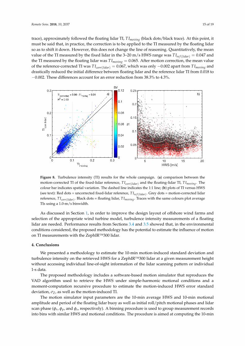
Analogously to Figure 5d, Figure 8a compares the TI of the floating lidar, TImoving, to themotion-corrected TI of the fixed-lidar reference, TIcorr(lidar). Dots are colour-coded according totheir spatial variation parameter. HWSs below 3 m/s, which are usually out of the production regimeof commercial wind turbines and tend to numerically distort the TI, were filtered out to enhance thereadability of the graph. Although some scattering is present in the pattern of dots, the regressionline (slope = 0.86, intercept = 0.01) shows a similar tendency to that of Figure 5d of approaching the1:1 line after motion correction. Quantitatively, by defining similar MD and RMSE indicators for theTI (counterpart of Equations (18) and (19) by changing standard deviation, σ, into TI), the MD forthe moving lidar reduced from 0.016 (uncorrected) to 0.003 (motion corrected). In terms of RMSE,the reduction was from 0.018 to 0.012, which despite being not very important implies an approximate30% reduction in the dispersion of data. In addition, most of the points falling far from the 1:1 line hadhigh spatial variation figures, typically SV > 0.06, which is characteristic of low HWS.

Figure 8b illustrates the successful application of the motion-correction algorithm bysuperimposing: (i) the TI measured by the uncorrected fixed-lidar reference (TIre f (lidar), red); (ii) theTI derived from the motion-corrected lidar reference (TIcorr(lidar), grey); and (iii) the TI measuredby the moving floating lidar (TImoving, black) as a function of the 10-min HWS. To aid visualinterpretation, average TIs using a 1.0 m/s binwidth were also plotted in red, white, and blacktraces, respectively. As expected, the apparent TI measured by the floating lidar (black trace) was higherthan the true one measured by the reference lidar (red trace). After application of motion correction tothe reference TI, TIre f (lidar) (red dots/red trace), the motion-corrected TI, TIcorr(lidar) (grey dots/white

Remote Sens. 2018, 10, 2037 15 of 19

trace), approximately followed the floating lidar TI, TImoving (black dots/black trace). At this point, itmust be said that, in practice, the correction is to be applied to the TI measured by the floating lidarso as to shift it down. However, this does not change the line of reasoning. Quantitatively, the meanvalue of the TI measured by the fixed lidar in the 3–20 m/s HWS range was TIre f (lidar) = 0.047 andthe TI measured by the floating lidar was TImoving = 0.065. After motion correction, the mean valueof the reference-corrected TI was TIcorr(lidar) = 0.067, which was only −0.002 apart from TImoving anddrastically reduced the initial difference between floating lidar and the reference lidar TI from 0.018 to−0.002. These differences account for an error reduction from 38.3% to 4.3%.

Figure 8. Turbulence intensity (TI) results for the whole campaign. (a) comparison between themotion-corrected TI of the fixed-lidar reference, TIcorr(lidar) and the floating-lidar TI, TImoving. Thecolour bar indicates spatial variation. The dashed line indicates the 1:1 line; (b) plots of TI versus HWS(see text): Red dots = uncorrected fixed-lidar reference, TIre f (lidar). Grey dots = motion-corrected lidarreference, TIcorr(lidar). Black dots = floating lidar, TImoving. Traces with the same colours plot averageTIs using a 1.0-m/s binwidth.

As discussed in Section 1, in order to improve the design layout of offshore wind farms andselection of the appropriate wind turbine model, turbulence intensity measurements of a floatinglidar are needed. Performance results from Sections 3.4 and 3.5 showed that, in the environmentalconditions considered, the proposed methodology has the potential to estimate the influence of motionon TI measurements with the ZephIR™300 lidar.

4. Conclusions

We presented a methodology to estimate the 10-min motion-induced standard deviation andturbulence intensity on the retrieved HWS for a ZephIR™300 lidar at a given measurement heightwithout accessing individual line-of-sight information of the lidar scanning pattern or individual1-s data.

The proposed methodology includes a software-based motion simulator that reproduces theVAD algorithm used to retrieve the HWS under simple-harmonic motional conditions and amoment-computation recursive procedure to estimate the motion-induced HWS error standarddeviation, σZ, as well as the motion-induced TI.

The motion simulator input parameters are the 10-min average HWS and 10-min motionalamplitude and period of the floating lidar buoy as well as initial roll/pitch motional phases and lidarscan phase (φr, φp, and φs, respectively). A binning procedure is used to group measurement recordsinto bins with similar HWS and motional conditions. The procedure is aimed at computing the 10-min

Remote Sens. 2018, 10, 2037 16 of 19

HWS error standard deviation in each bin by internally sweeping these phases in the [0, 2π) range,which therefore become blind inputs to the user.

The method relies on the approximation that roll/pitch amplitudes and periods are linearlycorrelated on a 10-min basis and that, consequently, only one motional amplitude and period is needed.This one-degree-of-freedom approximation combined with that of simple harmonic motion are themain limitations of the method. Under these hypotheses, the motion-induced HWS standard deviationwas proven to be independent of wind direction, which allows this variable to be neglected in thecomputations (wind direction errors caused by yaw motion are always corrected by means of thebuoy compass).

According to error-propagation laws, the motion-corrected HWS standard deviation (Equation (15)),which combines the motion-induced HWS error and the reference HWS, was shown to depend onthe correlation between these two variables and the degree of approximation by which it is estimated.Uncorrelated (ρ = 0) and linearly-correlated (|ρ| = 1) sub-cases were interpreted as upper and lowerbounds of the motion-corrected HWS standard deviation, respectively.

The performance of the proposed methodology was tested as part of a 60-day study period atoffshore metmast IJmuiden by using a sonic anemometer and a fixed lidar as reference instruments.The motion-corrected HWS standard deviation and that of the reference HWS (from either the fixedlidar or the sonic anemometer) were compared to the measured floating-lidar HWS standard deviationfor the 109 most frequent cases of the campaign. This indicated an overall improvement in the averageMD from 0.13 (uncorrected) to−0.03 m/s (motion corrected) and an average RMSE reduction from 0.17to 0.12 m/s, which essentially means that the floating-lidar and the motion-corrected HWS standarddeviation laid on the ideal 1:1 line with a dispersion equal to the RMSE.

When analysing the whole campaign as a function of the spatial variation, the most poorlycorrelated points were associated with mid-to-high spatial variations (SV > 0.06). Wider dispersionarose when using the sonic anemometer as reference, which was caused by the inherently differentwind measurement principle of the sonic as compared to the lidar. Analysis in terms of TI showedsimilar improvement, made evident by a reduction in the difference between the reference-lidar andthe floating-lidar TI from 0.018 (uncorrected) to −0.002 (motion corrected).

Despite these good results, they must be interpreted with caution because performance is based onMD and RMSE criteria over the whole statistical sample and not on an individual measurement basis.Overall, in the environmental conditions considered, the proposed methodology holds promise for usein the estimation of the influence of motion on TI measurements with the ZephIR™300 lidar. Theseresults should be extended to other conditions and set-ups, which, if proven effective, could eventuallybe used to correct TI measurements of floating lidars as standalone devices.

Author Contributions: This work was developed as part of M.A.G.-A.’s doctoral thesis supervised by F.R. andJ.T.-A. Development of the simulator (Section 2.2), analysis, and figures were done by M.A.G.-A. and J.T.-A.Database creation and binning was contributed by M.Sc. student A.S. Paper conceptualisation, mathematicalframework, and scientific text editing was completed by F.R.

Funding: This work was funded by the Spanish Ministry of Economy and Competitiveness (MEC)—EuropeanRegional Development (FEDER) funds under TEC2015-63832-P project and by European Union H2020, ACTRIS-2(GA-654109). CommSensLab is a “María de Maeztu” Unit of Excellence (MDM-2016-0600) funded by the AgenciaEstatal de Investigación, Spain.

Acknowledgments: The authors gratefully acknowledge LIM-UPC and EOLOS for the endless tests carried outat their premises and during the commissioning phase at IJmuiden (the Netherlands).

Conflicts of Interest: The authors declare no conflict of interest.

Remote Sens. 2018, 10, 2037 17 of 19

Abbreviations

The following abbreviations are used in this manuscript:

HWS Horizontal Wind SpeedLAT Lowest Astronomical TideMD Mean DifferenceSV Spatial VariationRMSE Root Mean Square ErrorTI Turbulence IntensityVAD Velocity–Azimuth DisplayWD Wind Direction

References

1. Global Wind Energy Council. Global Wind Energy Outlook 2016; Technical Report; Global Wind EnergyCouncil: Brussels, Belgium, 2016.

2. Global Wind Energy Council. Global Wind Energy Rerport 2016: Annual Market Update; Technical Report;Global Wind Energy Council: Brussels, Belgium, 2017.

3. Roland Berger. Offshore Wind toward 2020: On the Pathway to Cost Competitiveness; Technical Report; Roland Berger:Munich, Germany, 2013.

4. Barthelmie, R.; Pryor, S. Can Satellite Sampling of Offshore Wind Speeds Realistically Represent Wind SpeedDistributions? J. Appl. Meteorol. 2003, 42, 83–94. [CrossRef]

5. Chang, R.; Zhu, R.; Badger, M.; Hasager, C.B.; Zhou, R.; Ye, D.; Zhang, X. Applicability of Synthetic ApertureRadar wind retrievals on offshore wind resources assessment in Hangzhou Bay, China. Energies 2014,7, 3339–3354. [CrossRef]

6. Hirth, B.D.; Schroeder, J.L.; Gunter, W.S.; Guynes, J.G. Measuring a utility-scale turbine wake using theTTUKa mobile research radars. J. Atmos. Ocean. Technol. 2012, 29, 765–771. [CrossRef]

7. Barthelmie, R.; Folkerts, L.; Ormel, F.; Sanderhoff, P.; Eecen, P.; Stobbe, O.; Nielsen, N. Offshore wind turbinewakes measured by SODAR. J. Atmos. Ocean. Technol. 2003, 20, 466–477. [CrossRef]

8. Vogt, S.; Thomas, P. SODAR—A useful remote sounder to measure wind and turbulence. J. Wind Eng.Ind. Aerodyn. 1995, 54, 163–172. [CrossRef]

9. Lang, S.; McKeogh, E. LIDAR and SODAR Measurements of Wind Speed and Direction in Upland Terrainfor Wind Energy Purposes. Remote Sens. 2011, 3, 1871–1901. [CrossRef]

10. International Energy Association. State of the Art of Remote Wind Speed Sensing Techniques Using Sodar, Lidarand Satellites; Technical Report; International Energy Association: Paris, France, 2007.

11. Sempreviva, A.M.; Barthelmie, R.J.; Pryor, S.C. Review of Methodologies for Offshore Wind ResourceAssessment in European Seas. Surv. Geophys. 2008, 29, 471–497. [CrossRef]

12. Scholbrock, A.; Fleming, P.; Schlipf, D.; Wright, A.; Johnson, K.; Wang, N. Lidar-Enhanced Wind TurbineControl: Past, Present, and Future. In Proceedings of the 2016 American Control Conference (ACC), Boston,MA, USA, 6–8 July 2016; pp. 1399–1406.

13. Rodrigo, J.S. State-of-the-Art of Wind Resource Assessment. Deliverable D7, CENER, 2010. Available online:https://cordis.europa.eu/project/rcn/93290_en.html (accessed on 14 December 2012).

14. Clifton, A.; Courtney, M. 15. Ground-Based Vertically Profiling Remote Sensing for Wind Reource Assessment;Technical Report; IEA Wind Expert Group Study on Recommended Practices; IEA: Paris, France, 2013.

15. Li, J.; Yu, X.B. LiDAR technology for wind energy potential assessment: Demonstration and validation at asite around Lake Erie. Energy Convers. Manag. 2017, 144, 252–261. [CrossRef]

16. Trabucchi, D.; Trujillo, J.J.; Kühn, M. Nacelle-based Lidar Measurements for the Calibration of a Wake Model atDifferent Offshore Operating Conditions. Energy Procedia 2017, 137, 77–88. [CrossRef]

17. Krishnamurthy, R.; Reuder, J.; Svardal, B.; Fernando, H.; Jakobsen, J. Offshore Wind Turbine Wake characteristicsusing Scanning Doppler Lidar. Energy Procedia 2017, 137, 428–442. [CrossRef]

18. van Dooren, M.; Trabucchi, D.; Kühn, M. A Methodology for the Reconstruction of 2D Horizontal WindFields of Wind Turbine Wakes Based on Dual-Doppler Lidar Measurements. Remote Sens. 2016, 8, 809.[CrossRef]

Remote Sens. 2018, 10, 2037 18 of 19

19. International Electrotechnical Commission. IEC 61400-12 Wind Turbine Power Performance Testing; TechnicalReport; International Electrotechnical Commission: Geneva, Switzerland, 1998.

20. Williams, B.M. New Applications of Remote Sensing Technology for Offshore Wind Powert. Master’s Thesis,University Delawre, Newark, DE, USA, 2013.

21. Pichugina, Y.L.; Banta, R.M.; Brewer, W.A.; Sandberg, S.P.; Hardesty, R.M. Doppler Lidar–Based Wind-ProfileMeasurement System for Offshore Wind-Energy and Other Marine Boundary Layer Applications. J. Appl.Meteorol. Climatol. 2011, 51, 327–349. [CrossRef]

22. Courtney, M.S.; Hasager, C.B. Remote sensing technologies for measuring offshore wind. In Offshore WindFarms; Elsevier: Amsterdam, The Netherlands, 2016; Chapter 4, pp. 59–82.

23. Antoniou, I.; Jorgensen, H.E.; Mikkelsen, T.; Frandsen, S.; Barthelmie, R.; Perstrup, C.; Hurtig, M. Offshorewind profile measurements from remote sensing instruments. In Proceedings of the European Wind EnergyAssociation Conference & Exhibition, Athens, Greece, 27 February–2 March 2006.

24. Carbon Trust. Carbon Trust Offshore Wind Accelerator Roadmap for the Commercial Acceptance of Floating LIDARTechnology; Technical Report; Carbon Trust: London, UK, 2013.

25. Clifton, A.; Clive, P.; Gottschall, J.; Schlipf, D.; Simley, E.; Simmons, L.; Stein, D.; Trabucchi, D.; Vasiljevic, N.;Würth, I. IEA Wind Task 32: Wind Lidar Identifying and Mitigating Barriers to the Adoption of Wind Lidar.Remote Sens. 2018, 10, 406. [CrossRef]

26. Bischoff, O.; Wurth, I.; Gottschall, J.; Gribben, B.; Hughes, J.; Stein, D.; Verhoef, H. Recommended Practices forFloating Lidar Systems; Technical Report; IEA Wind Task 32; IEA: Paris, France, 2016.

27. Gottschall, J.; Wolken-Möhlmann, G.; Viergutz, T.; Lange, B. Results and conclusions of a floating-lidaroffshore test. Energy Procedia 2014, 53, 156–161. [CrossRef]

28. Schuon, F.; González, D.; Rocadenbosch, F.; Bischoff, O.; Jané, R. KIC InnoEnergy Project Neptune: Developmentof a Floating LiDAR Buoy for Wind, Wave and Current Measurements. In Proceedings of the DEWEK 2012German Wind Energy Conference, Bremen, Germany, 7–8 November 2012.

29. Sospedra, J.; Cateura, J.; Puigdefàbregas, J. Novel multipurpose buoy for offshore wind profile measurementsEOLOS platform faces validation at ijmuiden offshore metmast. Sea Technol. 2015, 56, 25–28.

30. Mathisen, J.P. Measurement of wind profile with a buoy mounted lidar. Energy Procedia 2013, 30, 12.31. Kyriazis, T. Low cost and flexible offshore wind measurements using a floating lidar solution (FLIDAR™).

In Proceedings of the EWEA Conference, Vienna, Austria, 4–7 February 2013.32. Hung, J.B.; Hsu, W.Y.; Chang, P.C.; Yang, R.Y.; Lin, T.H. The performance validation and operation of nearshore

wind measurements using the floating lidar. Coast. Eng. Proc. 2014, 1, 11. [CrossRef]33. Hsuan, C.Y.; Tasi, Y.S.; Ke, J.H.; Prahmana, R.A.; Chen, K.J.; Lin, T.H. Validation and Measurements of

Floating LiDAR for Nearshore Wind Resource Assessment Application. Energy Procedia 2014, 61, 1699–1702.[CrossRef]

34. Gottschall, J.; Gribben, B.; Stein, D.; Würth, I. Floating lidar as an advanced offshore wind speed measurementtechnique: Current technology status and gap analysis in regard to full maturity. Wiley Interdiscip. Rev.Energy Environ. 2017, 6. [CrossRef]

35. Gottschall, J.; Wolken-Möhlmann, G.; Lange, B. About offshore resource assessment with floating lidarswith special respect to turbulence and extreme events. J. Phys. Conf. Ser. 2014, 555, 012043. [CrossRef]

36. Mangat, M.; des Roziers, E.B.; Medley, J.; Pitter, M.; Barker, W.; Harris, M. The impact of tilt and inflowangle on ground based lidar wind measurements. In Proceedings of the EWEA 2014, Barcelona, Spain,10–13 March 2014.

37. Pitter, M.; Burin des Roziers, E.; Medley, J.; Mangat, M.; Slinger, C.; Harris, M. Performance Stability of Zephirin High Motion Enviroments: Floating and Turbine Mounted. Available online: https://bit.ly/2EuDY5i(accessed on 14 December 2018).

38. Wolken-Möhlmann, G.; Lilov, H.; Lange, B. Simulation of motion induced measurement errors for windmeasurements using LIDAR on floating platforms. Fraunhofer IWES Am Seedeich 2011, 45, 27572.

39. Bischoff, O.; Würth, I.; Cheng, P.; Tiana-Alsina, J.; Gutiérrez, M. Motion effects on lidar wind measurementdata of the EOLOS buoy. In Proceedings of the First International Conference on Renewable EnergiesOffshore, Lisbon, Portugal, 24–26 November 2014.

40. Tiana-Alsina, J.; Rocadenbosch, F.; Gutierrez-Antunano, M.A. Vertical Azimuth Display simulator forwind-Doppler lidar error assessment. In Proceedings of the 2017 IEEE International Geoscience and RemoteSensing Symposium (IGARSS), Fort Worth, TX, USA, 23–28 July 2017. [CrossRef]

Remote Sens. 2018, 10, 2037 19 of 19

41. Nicholls-Lee, R. A low motion floating platform for offshore wind resource assessment using Lidars.In Proceedings of the ASME 2013 32nd International Conference on Ocean, Offshore and Arctic Engineering,Nantes, France, 9–14 June 2013.

42. Tiana-Alsina, J.; Gutiérrez, M.A.; Würth, I.; Puigdefàbregas, J.; Rocadenbosch, F. Motion compensation studyfor a floating Doppler wind lidar. In Proceedings of the Geoscience and Remote Sensing Symposium, Milan,Italy, 26–31 July 2015.

43. Bischoff, O.; Schlipf, D.; Würth, I.; Cheng, P. Dynamic Motion Effects and Compensation Methods of aFloating Lidar Buoy. In Proceedings of the EERA DeepWind 2015 Deep Sea Offshore Wind Conference,Trondheim, Norway, 4–6 February 2015.

44. Gottschall, J.; Lilov, H.; Wolken-Möhlmann, G.; Lange, B. Lidars on floating offshore platforms; about thecorrection of motion-induced lidar measurement errors. In Proceedings of the EWEA 2012, Copenhagen,Denmark, 16–19 April 2012.

45. International Electrotechnical Commission. IEC 61400-1 2005 Wind Turbine Power Performance Testing; TechnicalReport; International Electrotechnical Commission: Geneva, Switzerland, 2005.

46. Manwell, J.F.; McGowan, J.G.; Rogers, A.L. Wind Energy Explained: Theory, Design and Application; NumberBook, Whole; Wiley: Chichester, UK, 2009.

47. Hansen, K.S.; Barthelmie, R.J.; Jensen, L.E.; Sommer, A. The impact of turbulence intensity and atmosphericstability on power deficits due to wind turbine wakes at Horns Rev wind farm. Wind Energy 2012, 15, 183–196.[CrossRef]

48. Sathe, A.; Mann, J.; Gottschall, J.; Courtney, M. Can wind lidars measure turbulence? J. Atmos. Ocean. Technol.2011, 28, 853–868. [CrossRef]

49. Sathe, A. Influence of Wind Conditions on Wind Turbine Loads and Measurements of Turbulence UsingLidars. Ph.D. Thesis, Delft University, Delft, The Netherlands, 2012.

50. Sathe, A.; Banta, R.; Pauscher, L.; Vogstad, K.; Schilpf, D.; Wylie, S. Estimating Turbulence Statistics andParameters from Ground- and Nacelle-Based Lidar Measurements; Technical Report; Technical University ofDenmark: Lyngby, Denmark, 2015.

51. Wagner, R.; Mikkelsen, T.; Courtney, M. Investigation of Turbulence Measurements With a Continuous Wave,Conically Scanning LiDAR; Technical Report; DTU: Lyngby, Denmark, 2009.

52. Henderson, S.W.; Gatt, P.; Rees, D.; Huffaker, M. Wind LIDAR. Laser Remote Sensing; Optical Science andEngineering; CRC Press: Boca Raton, FL, USA, 2005; Chapter 7.

53. Gutierrez-Antunano, M.A.; Tiana-Alsina, J.; Rocadenbosch, F.; Sospedra, J.; Aghabi, R.; Gonzalez-Marco, D.A wind-lidar buoy for offshore wind measurements: First commissioning test-phase results. In Proceedingsof the 2017 IEEE International Geoscience and Remote Sensing Symposium (IGARSS), Fort Worth, TX, USA,23–28 July 2017; doi:10.1109/igarss.2017.8127280.

54. Werkhoven, E.J.; Verhoef, J.P. Offshore Meteorological Mast Ijmuiden Abstract of Instrumentation Report.Available online: https://bit.ly/2PCjjxg (accessed on 14 December 2018).

55. Poveda, J.; Wouters, D.; Nederland, S.E.C. Wind Measurements at Meteorological Mast Ijmuiden. Availableonline: https://bit.ly/2QYbqHj (accessed on 14 December 2018).

56. Clifford, S.F.; Kaimal, J.C.; Lataitis, R.J.; Strauch, R.G. Ground-based remote profiling in atmospheric studies:An overview. Proc. IEEE 1994, 82, 313–355. [CrossRef]

57. Barlow, R.J. Statistics: A Guide to the Use of Statistical Methods in the Physical Sciences; Manchester PhysicsSeries, Wiley: Chichester, UK, 1989.

58. Papoulis, A. Probability, Random Variables, and Stochastic Processes; McGraw-Hill: New York, NY, USA, 1965.59. Gutiérrez-Antuñano, M.A.; Tiana-Alsina, J.; Rocadenbosch, F. Performance evaluation of a floating lidar

buoy in nearshore conditions. Wind Energy 2017, 20, 1711–1726. [CrossRef]

© 2018 by the authors. Licensee MDPI, Basel, Switzerland. This article is an open accessarticle distributed under the terms and conditions of the Creative Commons Attribution(CC BY) license (http://creativecommons.org/licenses/by/4.0/).