Evaluation of multiaxial stress-strain models and fatigue life … · 2015-03-17 · life prediction methods under proportional loading ... Brazil Abstract Multiaxial fatigue damage

Evaluation of multiaxial stress-strain models and fatiguelife prediction methods under proportional loading

Marco Antonio Meggiolaro, Jaime Tupiassú Pinho de CastroDepartment of Mechanical Engineering, Pontifical Catholic University of Rio de

Janeiro, Rio de Janeiro/RJ – Brazil

Antonio Carlos de Oliveira MirandaTecgraf, Pontifical Catholic University of Rio de Janeiro, Rio de Janeiro/RJ –

Brazil

Abstract

Multiaxial fatigue damage occurs when the principal stress directions vary during the loading induced byseveral independent forces, such as out-of-phase bending and torsion. Uniaxial damage models cannot bereliably applied in this case. Besides the need for multiaxial damage models, another key issue to reliablymodel such problems is how to calculate the elastic-plastic stresses from the multiaxial strains. Hooke’s lawcannot be used to correlate stresses and strains for short lives due to plasticity effects. Ramberg-Osgood cannotbe used either to directly correlate principal stresses and strains under multiaxial loading, because this modelhas been developed for the uniaxial case. The purpose of this work is to critically review and compare the mainfatigue crack initiation models under multiaxial loading. The studied models include stress-based ones suchas Sines, Findley and Dang Van, and strain-based ones such as the γN curve, Brown-Miller, Fatemi-Socie andSmith-Watson-Topper models. Modified formulations of the strain-based models are presented to incorporateFindley’s idea of using critical planes that maximize damage. To incorporate plasticity effects, four models arestudied and compared to correlate stresses and strains under proportional loading: the method of the highestKt, the constant ratio model, Hoffmann-Seeger’s and Dowling’s models.

Keywords: multiaxial fatigue, crack initiation, life prediction models, stress-strain models.

1 Introduction

Real loads can induce combined bending, torsional, axial and shear stresses, which can generate bi-or tri-axial variable stress/strain histories at the critical point (in general a notch root), causing theso-called multiaxial fatigue problems. The load history is said to be proportional when it generatesstresses with principal axes which maintain a fixed orientation, while non-proportional loading isassociated with principal directions which change in time during the loading history.

Mechanics of Solids in Brazil 2009, H.S. da Costa Mattos & Marcílio Alves (Editors)Brazilian Society of Mechanical Sciences and Engineering, ISBN 978-85-85769-43-7

366 M.A. Meggiolaro, J.T.P. de Castro and A.C.O. Miranda

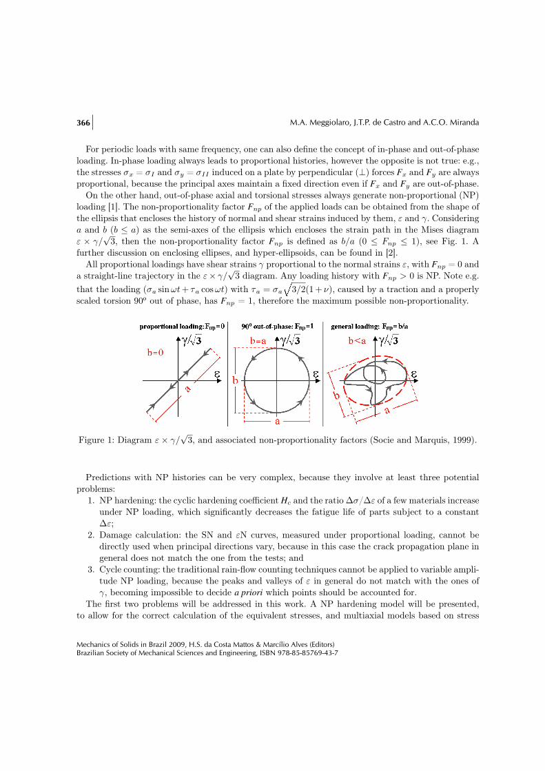
For periodic loads with same frequency, one can also define the concept of in-phase and out-of-phaseloading. In-phase loading always leads to proportional histories, however the opposite is not true: e.g.,the stresses σx = σI and σy = σII induced on a plate by perpendicular (⊥) forces Fx and Fy are alwaysproportional, because the principal axes maintain a fixed direction even if Fx and Fy are out-of-phase.

On the other hand, out-of-phase axial and torsional stresses always generate non-proportional (NP)loading [1]. The non-proportionality factor Fnp of the applied loads can be obtained from the shape ofthe ellipsis that encloses the history of normal and shear strains induced by them, ε and γ. Consideringa and b (b ≤ a) as the semi-axes of the ellipsis which encloses the strain path in the Mises diagramε × γ/

√3, then the non-proportionality factor Fnp is defined as b/a (0 ≤ Fnp ≤ 1), see Fig. 1. A

further discussion on enclosing ellipses, and hyper-ellipsoids, can be found in [2].All proportional loadings have shear strains γ proportional to the normal strains ε, with Fnp = 0 and

a straight-line trajectory in the ε× γ/√

3 diagram. Any loading history with Fnp > 0 is NP. Note e.g.that the loading (σa sin ωt+ τa cos ωt) with τa = σa

È3/2(1+ ν), caused by a traction and a properly

scaled torsion 90o out of phase, has Fnp = 1, therefore the maximum possible non-proportionality.

Figure 1: Diagram ε× γ/

√3, and associated non-proportionality factors (Socie and Marquis, 1999).

Predictions with NP histories can be very complex, because they involve at least three potentialproblems:

1. NP hardening: the cyclic hardening coefficient Hc and the ratio ∆σ/∆ε of a few materials increaseunder NP loading, which significantly decreases the fatigue life of parts subject to a constant∆ε;

2. Damage calculation: the SN and εN curves, measured under proportional loading, cannot bedirectly used when principal directions vary, because in this case the crack propagation plane ingeneral does not match the one from the tests; and

3. Cycle counting: the traditional rain-flow counting techniques cannot be applied to variable ampli-tude NP loading, because the peaks and valleys of ε in general do not match with the ones ofγ, becoming impossible to decide a priori which points should be accounted for.

The first two problems will be addressed in this work. A NP hardening model will be presented,to allow for the correct calculation of the equivalent stresses, and multiaxial models based on stress


Evaluation of stress-strain models and fatigue life prediction methods under proportional loading 367

or strain measurements will be used to calculate the damage generated both by proportional and NPloadings.

A few classical models that correlate stresses or strains with multiaxial fatigue life are studied below.Stress-based models (which can be applied for long life predictions) proposed by Sines, Findley andDang Van are presented, as well as strain-based models proposed by Brown-Miller, Fatemi-Socie andSmith-Watson-Topper (SWT), which must be used for short lives.

One problem with the application of the Fatemi-Socie or SWT models is the need to calculate theelastic-plastic stresses from the multiaxial strains, because Ramberg-Osgood is only valid for uniaxialstresses. Another challenge in multiaxial fatigue life calculations is the modeling of the notch effect.The elastic stress concentration factor Kσ and strain concentration factor Kε are the same for uniaxialloading, but in general in the multiaxial case Kσ is different from Kε even under elastic stresses.

Therefore, even in the elastic case, it is not trivial to study the notch effect under multiaxialloading. The problem is worse in the elastic-plastic case, where even uniaxial loadings can generateNP multiaxial stress and strain histories, due to the tri-axial stress state at the notch root andto the difference between the elastic and plastic Poisson coefficients. Typically, metallic alloys have1/4 ≤ νel ≤ 1/3 and νpl = 0.5. In the following sections the multiaxial stress-strain models arepresented and compared, including notch effects.

2 Non-proportional loading

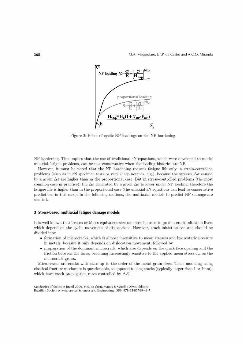
A few materials under NP cyclic loading can harden much more than it would be predicted fromthe traditional cyclic σε curve. This phenomenon, called NP hardening, depends on the load history(through the NP factor Fnp) and on the material (through a constant αnp of NP hardening, where0 ≤ αnp ≤ 1). The NP hardening can be modeled in general using the same Ramberg-Osgood plasticexponent hc from the uniaxial cyclic σ-ε curve, and using a new coefficient Hcnp = Hc ·(1 + αnp · Fnp),where Hc is the uniaxial Ramberg-Osgood plastic coefficient, see Fig. 2. Note that the NP hardeningcan multiply the uniaxial strain hardening coefficient Hc by a value as high as 2.

The largest NP hardening occurs when Fnp = 1, e.g. under a properly scaled traction-torsion loading90o out of phase which generates a circle in the ε× γ/

√3 Mises diagram.

Typically, the NP hardening effect is high in austenitic stainless steels at room temperature (αnp∼= 1

in the stainless steel 316), medium in carbon steels (αnp∼= 0.3 in the 1045 steel) and low in aluminum

alloys (αnp∼= 0 for Al 7075). Note that proportional histories do not lead to NP hardening.

The NP hardening happens in materials with low fault stacking energy (which in austenitic stainlesssteels is only 23mJ/m2) and well spaced dislocations, where the slip bands generated by proportionalloading are always planar. In these materials, the NP loads activate crossed slip bands in severaldirections (due to the rotation of the maximum shear planes), therefore increasing the hardeningeffect (αnp À 0) with respect to the proportional loadings. But in materials with high fault stackingenergy (such as aluminum alloys, with a typical value of 250mJ/m2) and with close dislocations,the crossed slip bands already happen naturally even under proportional loading, therefore the NPhistories do not cause any significant difference in hardening (αnp

∼= 0).But the Coffin-Manson or the Morrow crack initiation equations cannot account for the influence of



Figure 2: Effect of cyclic NP loadings on the NP hardening.

NP hardening. This implies that the use of traditional εN equations, which were developed to modeluniaxial fatigue problems, can be non-conservative when the loading histories are NP.

However, it must be noted that the NP hardening reduces fatigue life only in strain-controlledproblems (such as in εN specimen tests or very sharp notches, e.g.), because the stresses ∆σ causedby a given ∆ε are higher than in the proportional case. But in stress-controlled problems (the mostcommon case in practice), the ∆ε generated by a given ∆σ is lower under NP loading, therefore thefatigue life is higher than in the proportional case (the uniaxial εN equations can lead to conservativepredictions in this case). In the following sections, the multiaxial models to predict NP damage arestudied.

3 Stress-based multiaxial fatigue damage models

It is well known that Tresca or Mises equivalent stresses must be used to predict crack initiation lives,which depend on the cyclic movement of dislocations. However, crack initiation can and should bedivided into:

• formation of microcracks, which is almost insensitive to mean stresses and hydrostatic pressurein metals, because it only depends on dislocation movement; followed by

• propagation of the dominant microcrack, which also depends on the crack face opening and thefriction between the faces, becoming increasingly sensitive to the applied mean stress σm as themicrocrack grows.

Microcracks are cracks with sizes up to the order of the metal grain sizes. Their modeling usingclassical fracture mechanics is questionable, as opposed to long cracks (typically larger than 1 or 2mm),which have crack propagation rates controlled by ∆K.



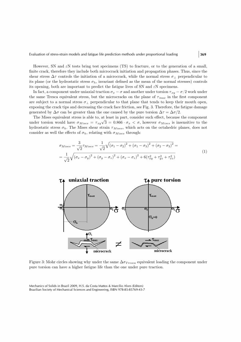
However, SN and εN tests bring test specimens (TS) to fracture, or to the generation of a small,finite crack, therefore they include both microcrack initiation and propagation phases. Thus, since theshear stress ∆τ controls the initiation of a microcrack, while the normal stress σ⊥ perpendicular toits plane (or the hydrostatic stress σh, invariant defined as the mean of the normal stresses) controlsits opening, both are important to predict the fatigue lives of SN and εN specimens.

In fact, a component under uniaxial traction σx = σ and another under torsion τxy = σ/2 work underthe same Tresca equivalent stress, but the microcracks on the plane of τmax in the first componentare subject to a normal stress σ⊥ perpendicular to that plane that tends to keep their mouth open,exposing the crack tips and decreasing the crack face friction, see Fig. 3. Therefore, the fatigue damagegenerated by ∆σ can be greater than the one caused by the pure torsion ∆τ = ∆σ/2.

The Mises equivalent stress is able to, at least in part, consider such effect, because the componentunder torsion would have σMises = τxy

√3 = 0.866 · σx < σ, however σMises is insensitive to the

hydrostatic stress σh. The Mises shear strain τMises, which acts on the octahedric planes, does notconsider as well the effects of σh, relating with σMises through:

σMises =3√2τMises =

1√2

È(σ1 − σ2)

2 + (σ1 − σ3)2 + (σ2 − σ3)

2 =

=1√2

q(σx − σy)2 + (σy − σz)

2 + (σx − σz)2 + 6(τ2

xy + τ2yz + τ2

xz)(1)

Figure 3: Mohr circles showing why under the same ∆σTresca equivalent loading the component underpure torsion can have a higher fatigue life than the one under pure traction.



Sines [3] has proposed a fatigue failure criterion under proportional multiaxial stresses, based on∆τMises and on σhm = (σxm + σym + σzm) /3, the hydrostatic component of the mean stresses (insen-sitive to the shear stresses):

∆τMises

2+ αS · (3 · σhm

) = βS (2)

where αS and βS are adjustable constants for each material, and

∆τMises =13

È(∆σ1 −∆σ2)

2 + (∆σ1 −∆σ3)2 + (∆σ2 −∆σ3)

2 (3)

In this way, according to the Sines criterion, a component will have infinite fatigue life underproportional loading if

∆τMises/2 + αS · (3 · σhm) < βS (4)

On the other hand, the Findley [4] criterion, which is also applicable to NP multiaxial loadings,assumes that the crack initiates at the critical plane of the critical point. This idea is interesting,because it is on this plane that the damage caused by the combination ∆τ/2 + αF · σ⊥ is maximum,where ∆τ/2 is the shear stress amplitude on that plane and σ⊥ is the normal stress perpendicular toit. Thus, according to Findley the fatigue failure criterion at the critical plane of the critical point is�

∆τ

2+ αF · σ⊥

�max

= βF (5)

where αF and βF are constants which must be fitted by measurements in at least two types of fatiguetests, e.g., under rotating bending and under pure torsion, or in push-pull tests under two different Rratios.

The critical plane can vary at each i-th event of the NP loads, even when the critical point remainsthe same, but Findley predicts fatigue failure based on the plane where the sum of the damagesassociated with [∆τ i (θ) /2 + αF · σ⊥i (θ)] is maximum, where θ is the angle of such plane with respectto a reference direction.

Under pure torsion, Eq. (5) can be written asÈ1 + α2

F ·∆τ

2= βF (6)

And under cyclic uniaxial traction with alternate component σa and maximum component σmax,it can be shown that Findley’s criterion can be written as

0.5σa

"Ê1 +

�2αF

1−R

�2

+2αF

1−R

#= βF (7)

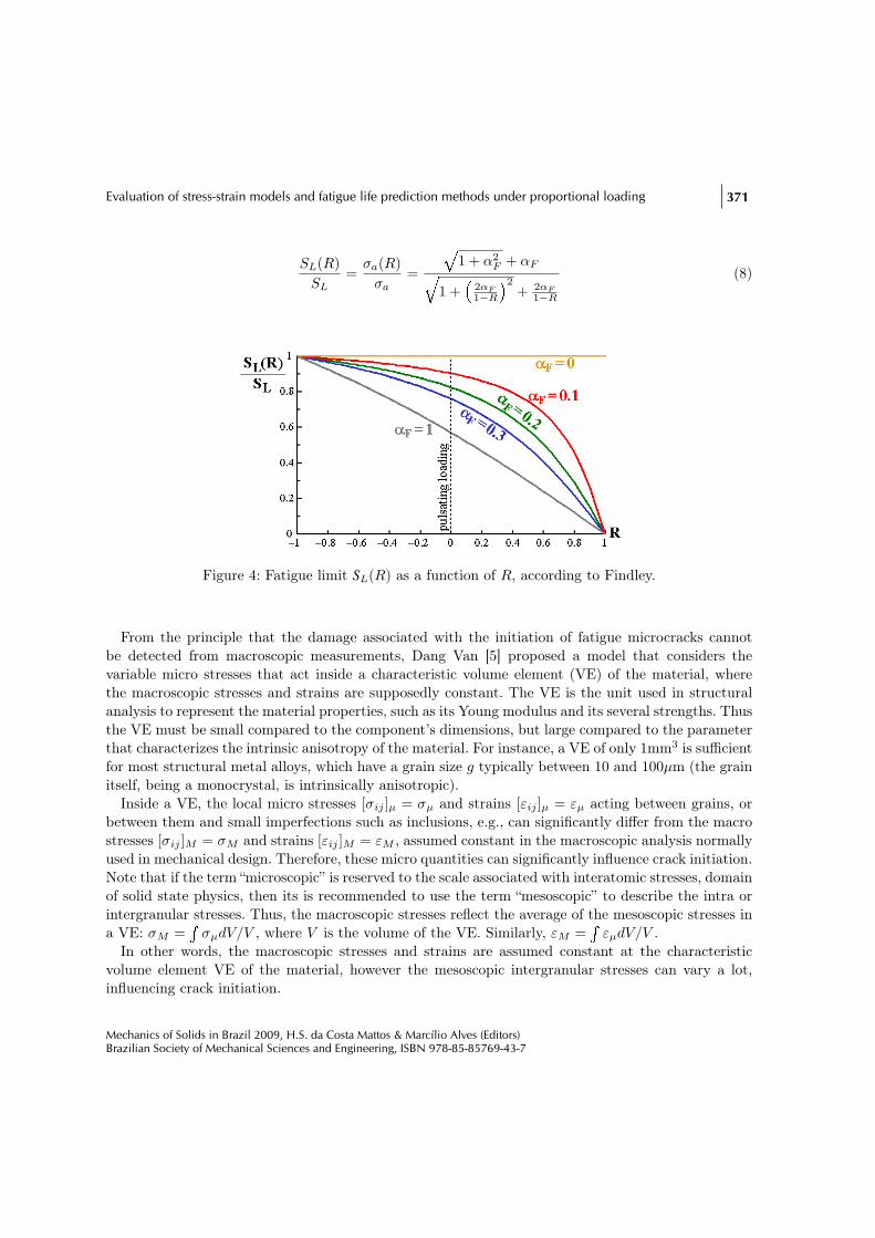
where R = σmin/σmax is the stress ratio, which quantifies the mean stress effects.Therefore, from Findley it is possible to estimate the fatigue limit SL(R) under any ratio R from

αF and the fatigue limit SL (obtained under zero mean loads, i.e., with R = −1, see Fig. 4) through



SL(R)SL

=σa(R)

σa=

È1 + α2

F + αFq1 +

�2αF

1−R

�2+ 2αF

1−R

(8)

Figure 4: Fatigue limit SL(R) as a function of R, according to Findley.

From the principle that the damage associated with the initiation of fatigue microcracks cannotbe detected from macroscopic measurements, Dang Van [5] proposed a model that considers thevariable micro stresses that act inside a characteristic volume element (VE) of the material, wherethe macroscopic stresses and strains are supposedly constant. The VE is the unit used in structuralanalysis to represent the material properties, such as its Young modulus and its several strengths. Thusthe VE must be small compared to the component’s dimensions, but large compared to the parameterthat characterizes the intrinsic anisotropy of the material. For instance, a VE of only 1mm3 is sufficientfor most structural metal alloys, which have a grain size g typically between 10 and 100µm (the grainitself, being a monocrystal, is intrinsically anisotropic).

Inside a VE, the local micro stresses [σij ]µ = σµ and strains [εij ]µ = εµ acting between grains, orbetween them and small imperfections such as inclusions, e.g., can significantly differ from the macrostresses [σij ]M = σM and strains [εij ]M = εM , assumed constant in the macroscopic analysis normallyused in mechanical design. Therefore, these micro quantities can significantly influence crack initiation.Note that if the term “microscopic” is reserved to the scale associated with interatomic stresses, domainof solid state physics, then its is recommended to use the term “mesoscopic” to describe the intra orintergranular stresses. Thus, the macroscopic stresses reflect the average of the mesoscopic stresses ina VE: σM =

RσµdV/V , where V is the volume of the VE. Similarly, εM =

RεµdV/V .

In other words, the macroscopic stresses and strains are assumed constant at the characteristicvolume element VE of the material, however the mesoscopic intergranular stresses can vary a lot,influencing crack initiation.



Since the microcracks initiate at persistent slip bands, Dang Van assumed that fatigue damage wascaused by the mesoscopic shear strain history τµ(t) and influenced by the mesoscopic hydrostatic stresshistory σµh(t). The simplest failure criterion involving these components is the linear combinationgiven by:

τµ(t) + αDV · σµh(t) = βDV (9)

Note that the Sines, Findley and Dang Van criteria can be included in the general class of Mohrmodels against material failure, which use combinations of the shear stress τ that acts on a certainplane with the normal or hydrostatic stresses σ on this plane:

τ + α · σ = β (10)

The Sines criterion uses the Mises or octahedric plane and the hydrostatic stresses, therefore τ ≡∆τMises/2, σ ≡ 3 · σhm, α ≡ αS , β ≡ βS ; Findley uses the shear stress on the critical plane and thenormal stress perpendicular to it, thus τ ≡ ∆τ/2, σ ≡ σ⊥, α ≡ αF , β ≡ βF ; and Dang Van can beobtained from τ ≡ τµ(t), σ ≡ σµh(t), α ≡ αDV , β ≡ βDV . Other similar criteria can be found in [1]and [6].

Finally, it is important to remember that the SN and εN tests involve both microcrack initiation(sensitive to τ) and propagation (more sensitive to σ) phases, and therefore fatigue damage can bemore influenced by τ or σ, depending on the percentage of the life spent at each phase. Therefore,materials with large values of α are more sensitive to σ (normal stresses are more important to them),probably spending more cycles to propagate than to initiate the microcrack.

4 Strain-based multiaxial fatigue damage models

The three multiaxial failure criteria presented above are based on macroscopic stresses that are sup-posedly elastic, therefore they are only applicable when σMises is much smaller than the cyclic yieldingstrength Syc. Thus, as in the case of the SN method, they should only be used to predict long fatiguelives. Otherwise, it is imperative to use fatigue damage criteria based on applied strains instead ofstresses [1], using the principles studied in the so-called εN method.

One of the simplest models is the one based on the γN curve, similar to Coffin-Manson’s equation,which uses the largest shear strain range ∆γmax acting on the specimen (γij ( 2εij , i 6= j) to predictfatigue life

∆γmax

2=

τc

G(2N)bγ + γc(2N)cγ (11)

where τ c, bγ , γc and cγ are parameters similar to the ones used in Coffin-Manson’s equation. In thisway, since the shear modulus G = E/ [2(1 + ν)], ν being Poisson’s coefficient, if no experimental datais available, then the γN curve can be estimated assuming τ c

∼= σc/√

3, bγ∼= b, γc

∼= εc

√3 and cγ

∼= c,resulting in



∆γmax

2∼= σc

E

2(1 + ν)√3

(2N)b + εc

√3(2N)c (12)

The γN curve is only recommended to model fatigue damage in materials that are more sensitiveto shear strains (which have small α in the Mohr models), and if the mean loads are zero. It would beexpected that such materials would have a shorter torsional fatigue life than similar materials moresensitive to normal stresses.

The Brown-Miller [7] model can consider the mean stress effects, combining the maximum range ofthe shear strain ∆γmax to the range of normal strain ∆ε⊥ (through the term ∆γmax/2 + αBM ·∆ε⊥)and the mean normal stress σ⊥m perpendicular to the plane of maximum shear strain, to obtain thefatigue life N :

∆γmax

2+ αBM ·∆ε⊥ = β1

σc − 2σ⊥m

E(2N)b + β2εc(2N)c (13)

where αBM is a fitting parameter (αBM∼= 0.3 for ductile metals in lives near the fatigue limit),

β1 = (1 + ν + (1− ν) · αBM , and β2 = 1.5 + 0.5 · αBM .This equation was adapted from Morrow to fit uniaxial traction test data, where the mean stress

σm is equal to 2σ⊥m (because σ⊥m acts perpendicularly to the plane of γmax, therefore it is worthhalf of σm).

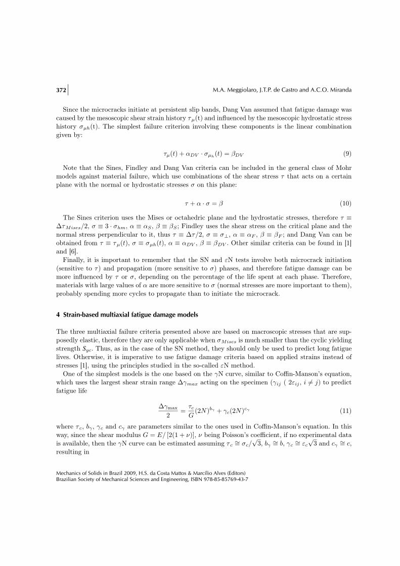
The values of β1 and β2 are obtained assuming uniaxial traction, see Fig. 5:

∆γmax = (1 + ν)∆ε

∆ε⊥ = (1− ν)∆ε/2

)⇒ ∆γmax

2+ αBM∆ε⊥ =

∆ε

2[(1 + ν) + αBM (1− ν)] (14)

Figure 5: Mohr circles for stresses and strains under uniaxial traction.



From Eq. (14), the coefficients β1 = (1 + ν) + (1− ν) ·αBM and β2 = 1.5 + 0.5 ·αBM are obtained,because ν = 0.5 for plastic strains, which preserve volume. The original Brown-Miller model assumesthat the elastic strains have ν = 0.3, therefore β1

∼= (1 + 0.3) + (1− 0.3) · αBM = 1.3 + 0.7 · αBM .The Brown-Miller model is frequently used in multiaxial fatigue, even though it is not reasonable to

assume that ∆ε⊥ can control the opening and closure of microcracks, because the range ∆ε does notinclude information about maximum stresses or strains. E.g., two microcracks with the same ∆γmax

and ∆ε⊥ can have very different fatigue lives if one is opened (under traction) and the other closed(under compression) due to the mean load effect. The use of σ⊥m compensates in part for this modelflaw, however the mean stress effect is only considered in the elastic part.

Fatemi and Socie [8] suggested replacing ∆ε⊥ by the maximum normal stress σ⊥max perpendicularto the plane of maximum shear strain, applying it to the γN curve:

∆γmax

2

�1 + αFS

σ⊥max

Syc

�=

τc

G(2N)bγ + γc(2N)cγ (15)

Note that the value of αBM and αFS indicates whether the material is more sensitive to τ (αBM

or αFS ¿ 1) or to σ (αBM or αFS À 1).If the propagation phase of the microcracks (more sensitive to σ) is dominant over initiation, the

Smith-Watson-Topper (SWT) multiaxial model can be used [9]:

∆ε1

2· σ⊥1 max =

σ2c

E(2N)2b + σcεc(2N)b+c (16)

where ∆ε1 is the range of the maximum principal strain and σ(1max is the stress peak in the directionperpendicular to ε1.

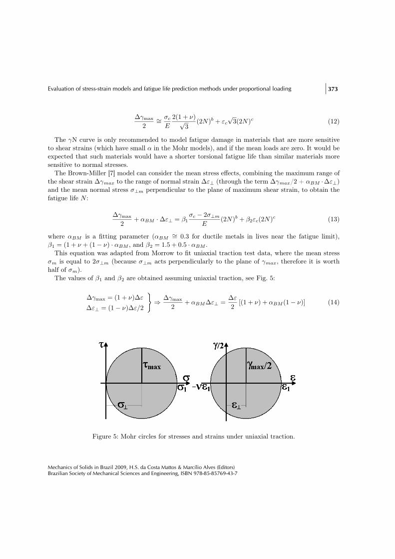
Figure 6 summarizes the parameters used in the above strain-based models. In addition, thereare several other models based on the plastic energy dissipated by the hysteresis loops, and othercombining energy with critical planes, see [1].

Figure 6: Parameters which affect the strain-based multiaxial models.

It is important to note that the plane of maximum shear strain amplitude ∆γmax/2 (used in Brown-Miller’s and Fatemi-Socie’s models) is in general different from the planes that would maximize therespective damage parameters (∆γ/2 + αBM (∆ε⊥ for Brown-Miller, and ∆γ((1 + αFS(σ⊥max/Syc)/2



for Fatemi-Socie). But if these are the parameters that cause damage, it is reasonable to argue thatfatigue life should be calculated on the critical plane that maximizes them (in a similar way as donein Findley’s model), and not on the plane of ∆γmax. In this way, it is a good idea to modify theBrown-Miller and Fatemi-Socie models introducing a subtle but important change:

∆γmax

2+ αBM ·∆ε⊥ ⇒

�∆γ

2+ αBM ·∆ε⊥

�max

(17)

∆γmax

2

�1 + αFS

σ⊥max

Syc

�⇒�

∆γ

2+ αFS

∆γ

2σ⊥γ

Syc

�max

(18)

The use of critical planes that maximize the damage parameters in each model has the advantage ofpredicting not only the fatigue life but also the dominant planes where the crack will initiate. However,these calculations are not simple and require the use of sophisticated numerical methods.

This idea can also be applied to the SWT model, calculating the critical plane where the productbetween the normal strain range ∆ε⊥ and the normal stress peak σ⊥max is maximized, adopting themodification

∆ε1

2· σ⊥1 max ⇒

�∆ε⊥

2· σ⊥max

�max

(19)

A great advantage of the Fatemi-Socie (or SWT) model is to be able to consider the effect of NPhardening from the peak of normal stress σ⊥max (or σ⊥1max). In stainless steels, e.g., a NP historyleads to a much higher damage than a proportional one with the same ∆γmax and ∆ε⊥, because theNP hardening increases the value of σ⊥max (or σ⊥1max). Note that Brown-Miller would wrongfullypredict the same damage in both histories (because ∆γmax and ∆ε⊥ would be the same), and onlythe Fatemi-Socie and SWT models would be able to correctly account for the greater damage of theNP loading (assuming that Hcnp would be used to obtain σ⊥max and σ⊥1max).

5 Multiaxial stress-strain relations

Hooke’s law cannot be used to correlate stresses and strains for short multiaxial fatigue life predictions,due to plasticity effects. The hookean stresses and strains, σ̃ and ε̃, defined as the values of σ and ε

obtained assuming that the material would be linear elastic (using Hooke’s law and, at the notches,considering elastic Kσ and Kε), can only be applied for long life predictions.

In addition, Ramberg-Osgood cannot be used either to directly correlate principal stresses andstrains σi and εi (i = 1, 2, 3) of a multiaxial history, because this model has been developed for theuniaxial case.

However, if the elastic nominal stress range ∆σn is caused by in-phase loading, then it is trivial tocalculate the elastic-plastic stresses and strains at the notch root using the “highest Kt method”. In thisapproximate method, the equivalent nominal stress range ∆σn calculated from Tresca or Mises is usedto obtain ∆σ and ∆ε at the notch root using Ramberg-Osgood and (for safety, because the methodis conservative) the highest Kt in Neuber’s rule. Remember that the multiaxial loadings can result, at



the same notch root, in different values of Kt for traction, bending, torsion and shear loadings, butonly the maximum one is used. To generate more accurate predictions for notches under combinedstresses, it is recommended to use multiaxial σ-ε relations.

Several models have been proposed to correlate σi and εi in proportional histories, e.g.: the constantratio model [1], Hoffmann-Seeger’s model ([10], and Dowling’s model [11]. To present these threemodels, it is necessary to define a few variables involved in their formulation:

• σ̃1, σ̃2, σ̃3, ε̃1, ε̃2, ε̃3: hookean principal stresses and strains at the notch root (elastically calcu-lated using Hooke’s law and elastic Kσ and Kε);

• σ̃Mises, ε̃Mises: hookean Mises stress and strain (at the notch root), calculated using the abovevariables;

• σ1, σ2, σ3, ε1, ε2, ε3: elastic-plastic principal stresses and strains (notch root);• σMises, εMises: Mises stress and strain (notch root);• λ2, λ3: ratios between pairs of principal stresses, where λ2 = σ2/σ1 and λ3 = σ3/σ1, both

between -1 and 1;• ϕ2, ϕ3: ratios between pairs of principal strains, where ϕ2 = ε2/ε1, ϕ3 = ε3/ε1, both between

-1 and 1; and• λMises, ϕMises: Mises ratios λMises = σMises/σ1 and ϕMises = εMises/ε1.

From the above definitions, it is possible to obtain

λMises =σMises

σ1=

1√2

È(1− λ2)

2 + (1− λ3)2 + (λ2 − λ3)

2 (20)

φMises =εMises

ε1=

1√2(1 + ν)

È(1− φ2)

2 + (1− φ3)2 + (φ2 − φ3)

2 (21)

The three models are described next.

5.1 Constant ratio model

The constant ratio model [1] assumes that, under a proportional history, the bi-axial ratios λ2, λ3, ϕ2

and ϕ3 remain constant even after yielding has occurred. Since the elastic Poisson coefficient νel istypically between 1/4 and 1/3 in most metal alloys, significantly different than the plastic νpl = 0.5,these ratios are in fact not constant, but for small plastic strains this is a good approximation.

Thus, these ratios can be estimated from the elastic (hookean) stresses and strains, obtained fromHooke’s law using elastic Kσ and Kε:

λ2∼= σ̃2

σ̃1, λ3

∼= σ̃3

σ̃1, φ2

∼= ε̃2

ε̃1, φ3

∼= ε̃3

ε̃1(22)

Therefore, λMises is also a constant, leading to

λMises∼= σ̃Mises

σ̃1⇒ σ̃Mises

∼= σ̃1√2

È(1− λ2)

2 + (1− λ3)2 + (λ2 − λ3)

2 (23)

and, similarly, ϕMises can be calculated from ϕ2 and ϕ3. The cyclic σ-ε relation is then defined usingMises and the Ramberg-Osgood uniaxial parameters



εMises =σMises

E+�

σMises

Hc

�1/hc

(24)

If no notches are present, then the above equation is used together with the estimates for λMises,ϕMises, λ2, λ3, ϕ2 and ϕ3 to obtain σi from εi (i = 1, 2, 3), or vice-versa. In notched components,σ̃Mises (elastically calculated including the Kts) is applied to a variation of the Neuber’s rule tocalculate the Mises elastic-plastic stress σMises and, finally, εMises, σi and εi (i = 1, 2, 3):

(σ̃Mises)2

E= σMises · εMises =

(σMises)2

E+ σMises ·

�σMises

Hc

�1/hc

(25)

After calculating σMises and εMises, the constant ratio model obtains the principal stress and strainusing: (

σ1 = σMises/λMises, σ2 = λ2σ1, σ3 = λ3σ1

ε1 = εMises/φMises, ε2 = φ2ε1, ε3 = φ3ε1

(26)

5.2 Hoffmann-Seeger’s model

Hoffmann-Seeger’s model [10] uses the same cyclic σ-ε relation and the same variation of Neuber’srule presented above to calculate σMises and εMises, but it assumes that:

• the critical point happens at the surface, with principal stresses σ1 and σ2;• σ3 is defined normal to the surface, therefore σ3 = 0 (and then λ3 = 0); and• only the ratio φ2 = ε̃2/ε̃1 is estimated using the linear elastic (hookean) values.

After calculating σMises and εMises, σi and εi are estimated from:(σ1 = σMises/λ̄Mises, σ2 = λ̄2σ1, σ3 = 0

ε1 = (1−λ̄2ν̄)εMises

λ̄Mises, ε2 = φ2ε1, ε3 = −ν̄ε1

1+λ̄21−λ̄2ν̄

(27)

ν̄ =12− (1/2− νel)σMises

E · εMises, λ̄2 =

φ2 + ν̄

1 + φ2ν̄, λ̄Mises =

È1− λ̄2 + λ̄2

2 (28)

5.3 Dowling’s model

The model proposed in [11] also assumes that the principal stresses σ1 and σ2 act on the surface ofthe critical point (therefore σ3 is zero), and it considers λ2 and ϕ2 constant, estimating them fromtheir hookean values

λ2 =σ2

σ1

∼= σ̃2

σ̃1

∼= φ2 + ν

1 + φ2ν, φ2 =

ε2

ε1

∼= ε̃2

ε̃1

∼= λ2 − ν

1− λ2ν(29)

Exceptionally, σ2 is defined here as the lowest principal stress at the surface, even if σ2 is smallerthan σ3 (i.e. the convention σ3 ≤ σ2 ≤ σ1 is violated if λ2 < 0).



The greatest difference between the previous two models and Dowling’s is that the latter correlatesσ1 and ε1 directly using effective Ramberg-Osgood parameters E∗ and H∗

c

E∗ =�

1 + φ2ν

1− ν2

�· E, H∗

c = Hc ·�

22− λ2

�hc

(1− λ2 + λ22)0.5(hc−1) (30)

and the effective relation between σ1 and ε1 is [11]

ε1 =σ1

E∗ +�

σ1

Hc∗

�1/hc

(31)

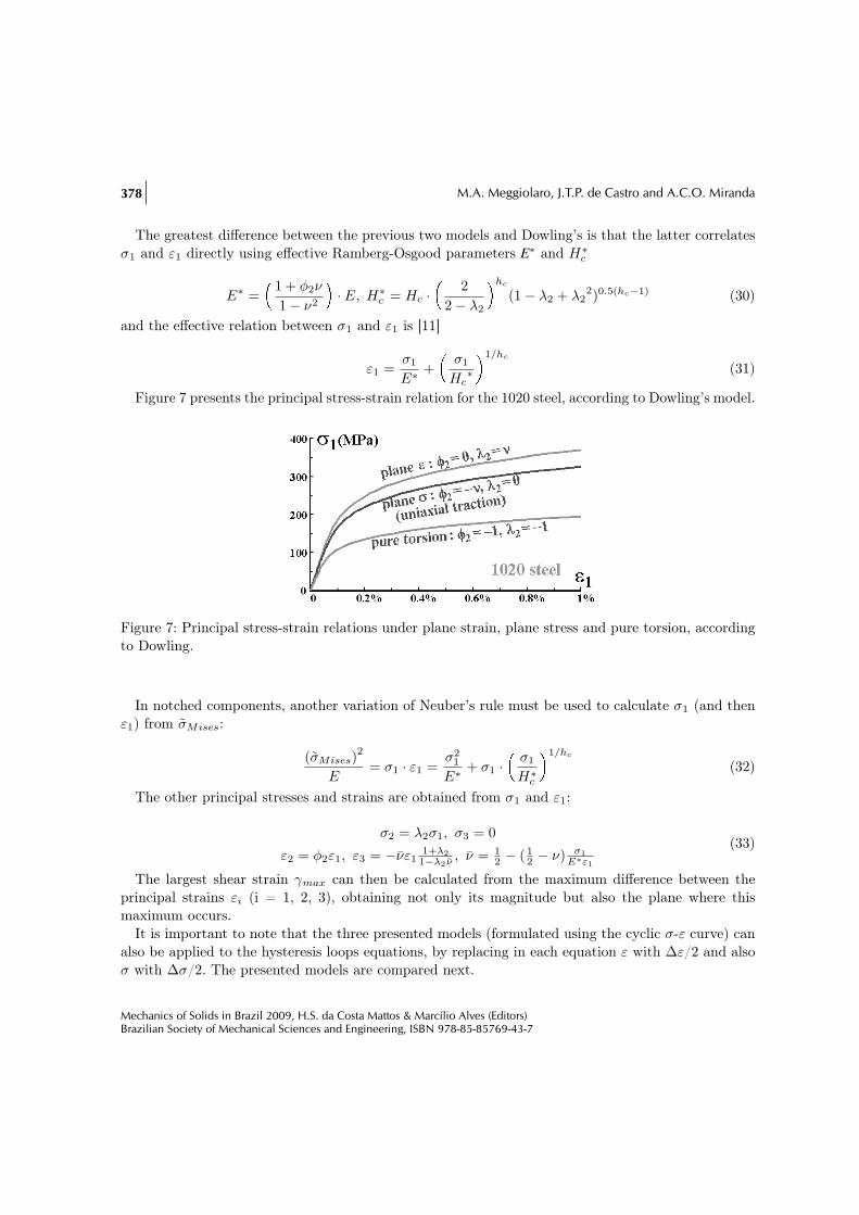
Figure 7 presents the principal stress-strain relation for the 1020 steel, according to Dowling’s model.

Figure 7: Principal stress-strain relations under plane strain, plane stress and pure torsion, accordingto Dowling.

In notched components, another variation of Neuber’s rule must be used to calculate σ1 (and thenε1) from σ̃Mises:

(σ̃Mises)2

E= σ1 · ε1 =

σ21

E∗ + σ1 ·�

σ1

H∗c

�1/hc

(32)

The other principal stresses and strains are obtained from σ1 and ε1:

σ2 = λ2σ1, σ3 = 0

ε2 = φ2ε1, ε3 = −ν̄ε11+λ21−λ2ν̄ , ν̄ = 1

2 − ( 12 − ν) σ1

E∗ε1

(33)

The largest shear strain γmax can then be calculated from the maximum difference between theprincipal strains εi (i = 1, 2, 3), obtaining not only its magnitude but also the plane where thismaximum occurs.

It is important to note that the three presented models (formulated using the cyclic σ-ε curve) canalso be applied to the hysteresis loops equations, by replacing in each equation ε with ∆ε/2 and alsoσ with ∆σ/2. The presented models are compared next.



6 Comparison among the multiaxial models

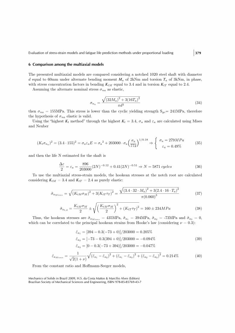
The presented multiaxial models are compared considering a notched 1020 steel shaft with diameterd equal to 60mm under alternate bending moment Ma of 2kNm and torsion Ta of 3kNm, in phase,with stress concentration factors in bending KtM equal to 3.4 and in torsion KtT equal to 2.4.

Assuming the alternate nominal stress σna as elastic,

σna=

È(32Ma)2 + 3(16Ta)2

πd3(34)

then σna = 155MPa. This stress is lower than the cyclic yielding strength Syc= 241MPa, thereforethe hypothesis of σna elastic is valid.

Using the “highest Kt method” through the highest Kt = 3.4, σa and εa are calculated using Misesand Neuber

(Ktσna)2 = (3.4 · 155)2 = σaεaE = σa2 + 203000 · σa

� σa

772

�1/0.18

⇒(

σa = 279MPa

εa = 0.49%(35)

and then the life N estimated for the shaft is

∆ε

2= εa =

896203000

(2N)−0.12 + 0.41(2N)−0.51 ⇒ N = 5871 cycles (36)

To use the multiaxial stress-strain models, the hookean stresses at the notch root are calculatedconsidering KtM = 3.4 and KtT = 2.4 as purely elastic:

σ̃aMises=È

(KtMσM )2 + 3(KtT τT )2 =

È(3.4 · 32 ·Ma)2 + 3(2.4 · 16 · Ta)2

π(0.060)3(37)

σ̃a1,2 =KtMσM

2±Ê�

KtMσM

2

�2

+ (KtT τT )2 = 160± 234MPa (38)

Thus, the hookean stresses are σ̃aMises= 435MPa, σ̃a1 = 394MPa, σ̃a2 = -73MPa and σ̃a3 = 0,

which can be correlated to the principal hookean strains from Hooke’s law (considering ν = 0.3):

ε̃a1 = [394− 0.3(−73 + 0)]/203000 = 0.205%

ε̃a2 = [−73− 0.3(394 + 0)]/203000 = −0.094%

ε̃a3 = [0− 0.3(−73 + 394)]/203000 = −0.047%

(39)

ε̃aMises=

1√2(1 + ν)

È(ε̃a1 − ε̃a2)

2 + (ε̃a1 − ε̃a3)2 + (ε̃a2 − ε̃a3)

2 = 0.214% (40)

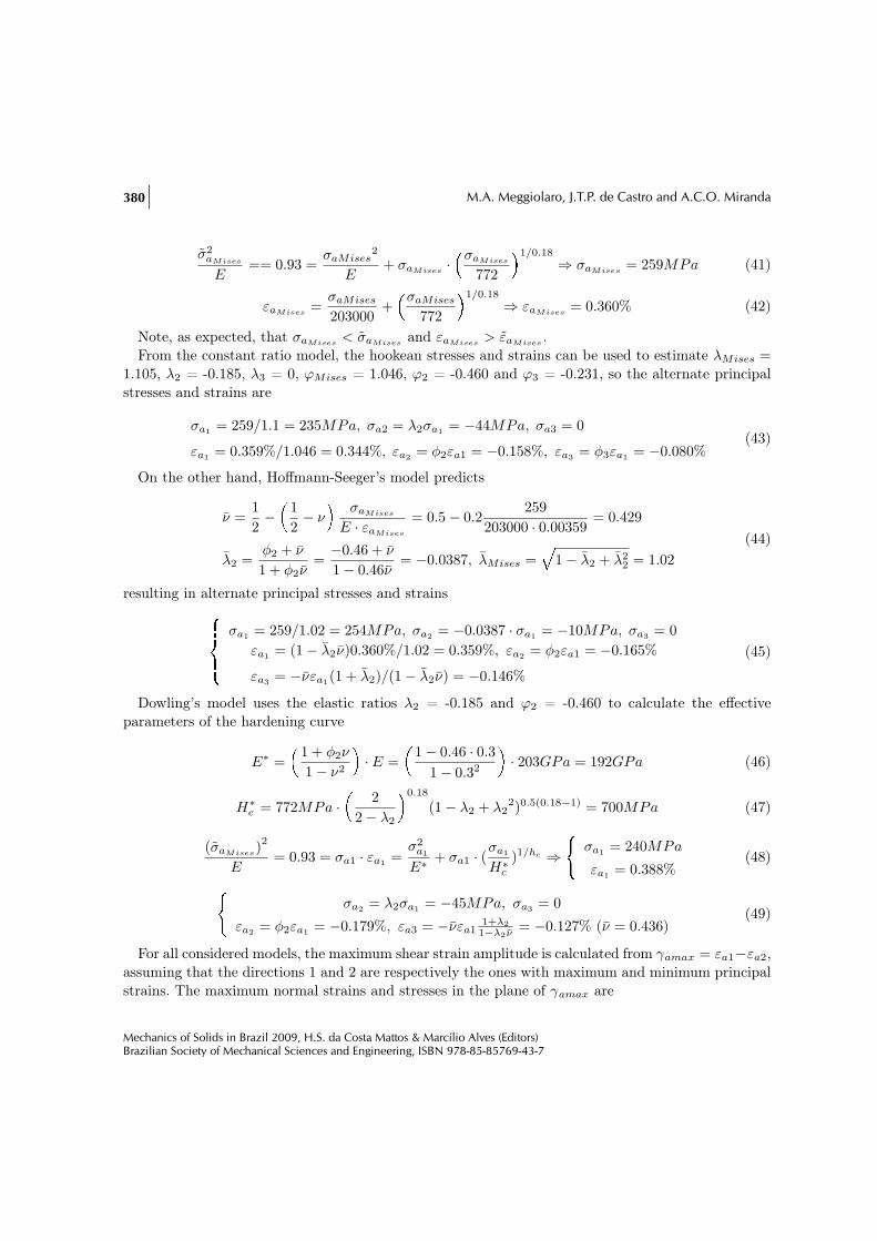
From the constant ratio and Hoffmann-Seeger models,



σ̃2aMises

E== 0.93 =

σaMises2

E+ σaMises

·�σaMises

772

�1/0.18

⇒ σaMises= 259MPa (41)

εaMises=

σaMises

203000+�σaMises

772

�1/0.18

⇒ εaMises= 0.360% (42)

Note, as expected, that σaMises< σ̃aMises

and εaMises> ε̃aMises

.From the constant ratio model, the hookean stresses and strains can be used to estimate λMises =

1.105, λ2 = -0.185, λ3 = 0, ϕMises = 1.046, ϕ2 = -0.460 and ϕ3 = -0.231, so the alternate principalstresses and strains are

σa1 = 259/1.1 = 235MPa, σa2 = λ2σa1 = −44MPa, σa3 = 0

εa1 = 0.359%/1.046 = 0.344%, εa2 = φ2εa1 = −0.158%, εa3 = φ3εa1 = −0.080%(43)

On the other hand, Hoffmann-Seeger’s model predicts

ν̄ =12−�

12− ν

�σaMises

E · εaMises

= 0.5− 0.2259

203000 · 0.00359= 0.429

λ̄2 =φ2 + ν̄

1 + φ2ν̄=−0.46 + ν̄

1− 0.46ν̄= −0.0387, λ̄Mises =

È1− λ̄2 + λ̄2

2 = 1.02(44)

resulting in alternate principal stresses and strains8><>: σa1 = 259/1.02 = 254MPa, σa2 = −0.0387 · σa1 = −10MPa, σa3 = 0εa1 = (1− λ̄2ν̄)0.360%/1.02 = 0.359%, εa2 = φ2εa1 = −0.165%

εa3 = −ν̄εa1(1 + λ̄2)/(1− λ̄2ν̄) = −0.146%

(45)

Dowling’s model uses the elastic ratios λ2 = -0.185 and ϕ2 = -0.460 to calculate the effectiveparameters of the hardening curve

E∗ =�

1 + φ2ν

1− ν2

�· E =

�1− 0.46 · 0.3

1− 0.32

�· 203GPa = 192GPa (46)

H∗c = 772MPa ·

�2

2− λ2

�0.18

(1− λ2 + λ22)0.5(0.18−1) = 700MPa (47)

(σ̃aMises)2

E= 0.93 = σa1 · εa1 =

σ2a1

E∗ + σa1 · (σa1

H∗c

)1/hc ⇒(

σa1 = 240MPa

εa1 = 0.388%(48)(

σa2 = λ2σa1 = −45MPa, σa3 = 0

εa2 = φ2εa1 = −0.179%, εa3 = −ν̄εa11+λ21−λ2ν̄ = −0.127% (ν̄ = 0.436)

(49)

For all considered models, the maximum shear strain amplitude is calculated from γamax = εa1−εa2,assuming that the directions 1 and 2 are respectively the ones with maximum and minimum principalstrains. The maximum normal strains and stresses in the plane of γamax are



εa⊥ = (εa1 + εa2)/2 and σa⊥ = (σa1 + σa2)/2 (50)

Since in this problem the mean stresses and strains are zero, the values used by the Brown-Miller,Fatemi-Socie and SWT strain-life models are respectively ∆ε⊥ = 2εa⊥, σ⊥max = σa⊥ and σ⊥1max =σa1 .

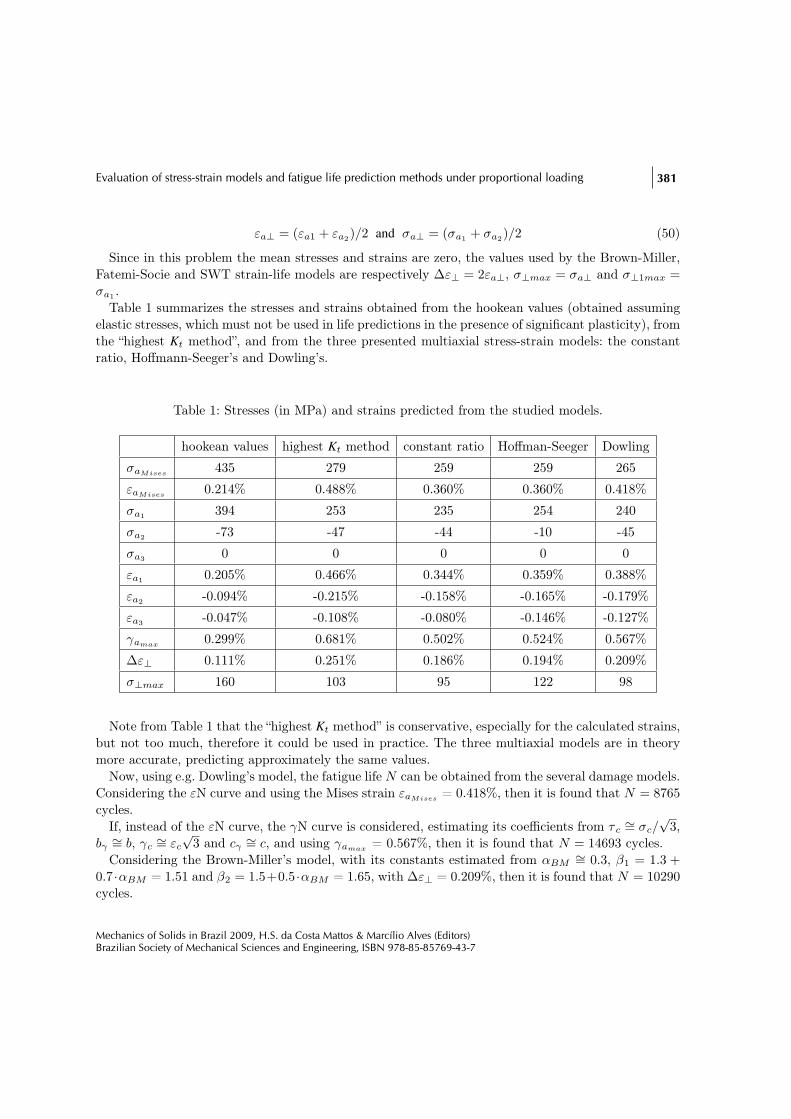
Table 1 summarizes the stresses and strains obtained from the hookean values (obtained assumingelastic stresses, which must not be used in life predictions in the presence of significant plasticity), fromthe “highest Kt method”, and from the three presented multiaxial stress-strain models: the constantratio, Hoffmann-Seeger’s and Dowling’s.

Table 1: Stresses (in MPa) and strains predicted from the studied models.

hookean values highest Kt method constant ratio Hoffman-Seeger Dowling

σaMises 435 279 259 259 265

εaMises0.214% 0.488% 0.360% 0.360% 0.418%

σa1 394 253 235 254 240

σa2 -73 -47 -44 -10 -45

σa3 0 0 0 0 0

εa1 0.205% 0.466% 0.344% 0.359% 0.388%

εa2 -0.094% -0.215% -0.158% -0.165% -0.179%

εa3 -0.047% -0.108% -0.080% -0.146% -0.127%

γamax 0.299% 0.681% 0.502% 0.524% 0.567%

∆ε⊥ 0.111% 0.251% 0.186% 0.194% 0.209%

σ⊥max 160 103 95 122 98

Note from Table 1 that the “highest Kt method” is conservative, especially for the calculated strains,but not too much, therefore it could be used in practice. The three multiaxial models are in theorymore accurate, predicting approximately the same values.

Now, using e.g. Dowling’s model, the fatigue life N can be obtained from the several damage models.Considering the εN curve and using the Mises strain εaMises

= 0.418%, then it is found that N = 8765cycles.

If, instead of the εN curve, the γN curve is considered, estimating its coefficients from τ c∼= σc/

√3,

bγ∼= b, γc

∼= εc

√3 and cγ

∼= c, and using γamax = 0.567%, then it is found that N = 14693 cycles.Considering the Brown-Miller’s model, with its constants estimated from αBM

∼= 0.3, β1 = 1.3 +0.7 ·αBM = 1.51 and β2 = 1.5+0.5 ·αBM = 1.65, with ∆ε⊥ = 0.209%, then it is found that N = 10290cycles.



Fatemi-Socie’s model, using αFS∼= Syc/σc = 241MPa/896MPa ∼= 0.27 and the γN curve estimated

as above, where σ⊥max = 98MPa, results in N = 11201 cycles.And finally, considering the SWT’s model, which is appropriate for materials more sensitive to

normal stresses, with ∆ε1/2 = εa1 = 0.388% and, since the mean loads are zero, σ⊥1max = σa1 =240MPa, then N = 13577 cycles.

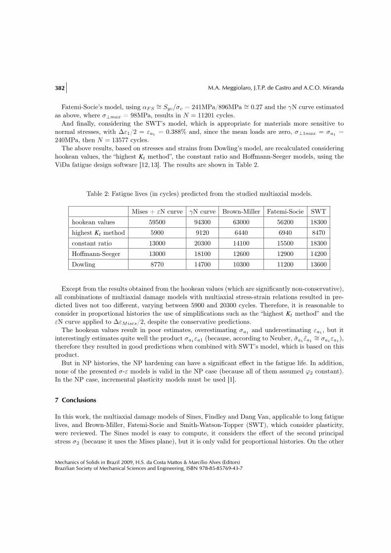
The above results, based on stresses and strains from Dowling’s model, are recalculated consideringhookean values, the “highest Kt method”, the constant ratio and Hoffmann-Seeger models, using theViDa fatigue design software [12, 13]. The results are shown in Table 2.

Table 2: Fatigue lives (in cycles) predicted from the studied multiaxial models.

Mises + εN curve γN curve Brown-Miller Fatemi-Socie SWT

hookean values 59500 94300 63000 56200 18300

highest Kt method 5900 9120 6440 6940 8470

constant ratio 13000 20300 14100 15500 18300

Hoffmann-Seeger 13000 18100 12600 12900 14200

Dowling 8770 14700 10300 11200 13600

Except from the results obtained from the hookean values (which are significantly non-conservative),all combinations of multiaxial damage models with multiaxial stress-strain relations resulted in pre-dicted lives not too different, varying between 5900 and 20300 cycles. Therefore, it is reasonable toconsider in proportional histories the use of simplifications such as the “highest Kt method” and theεN curve applied to ∆εMises/2, despite the conservative predictions.

The hookean values result in poor estimates, overestimating σa1 and underestimating εa1 , but itinterestingly estimates quite well the product σa1εa1 (because, according to Neuber, σ̃a1 ε̃a1

∼= σa1εa1),therefore they resulted in good predictions when combined with SWT’s model, which is based on thisproduct.

But in NP histories, the NP hardening can have a significant effect in the fatigue life. In addition,none of the presented σ-ε models is valid in the NP case (because all of them assumed ϕ2 constant).In the NP case, incremental plasticity models must be used [1].

7 Conclusions

In this work, the multiaxial damage models of Sines, Findley and Dang Van, applicable to long fatiguelives, and Brown-Miller, Fatemi-Socie and Smith-Watson-Topper (SWT), which consider plasticity,were reviewed. The Sines model is easy to compute, it considers the effect of the second principalstress σ2 (because it uses the Mises plane), but it is only valid for proportional histories. On the other



hand, Findley’s model is hard to compute, because it requires the search for a critical plane, but forlong lives it is valid for any load history, proportional or NP. Dang Van’s model is able to considerthe damage in a mesoscopic scale, but it has the limitations of the stress-based models.

The strain-based models are valid for any life, short or long. Among them, the Brown-Miller andFatemi-Socie models give more value to the shear strains γ, while SWT does it for normal strainsε. Brown-Miller and Fatemi-Socie combine ∆γmax to ∆ε⊥ or to σ⊥max normal to the direction ofγmax, being applicable to proportional or NP histories. SWT uses the principal strain ε1. The mostversatile models among the studied ones are the Fatemi-Socie and SWT, because they can include theNP hardening effect. But in order to generate a more realistic model, it is important to modify thesecriteria to calculate the fatigue life in the critical plane where the damage parameters of each modelare maximized.

The main multiaxial stress-strain models were also reviewed and compared. It can be concludedthat multiaxial stress-strain relations must be used instead of uniaxial ones, even though a few sim-plifications are adequate, such as the “highest Kt method” for notched components. Since the criticalpoint of a structure is usually in its surface, in general a 2D analysis (under plane stress) is enoughfor multiaxial fatigue design. Except for the results from the hookean values, which are significantlynon-conservative, all combinations of strain-based multiaxial damage models with multiaxial stress-strain relations resulted in not too different lives (within a factor of 2) for the considered example,which has significant plastic strains (but they were not much higher than the elastic ones). The bestpredictions should be the ones from multiaxial models that use the critical plane idea, where thedamage parameters are maximized. However, none of the studied stress-strain models is valid for NPhardening, which can have a significant influence in the fatigue lives of e.g. stainless steels.

References

[1] Socie, D.F. & Marquis, G.B., Multiaxial fatigue. SAE International, 1999.[2] Zouain, N., Mamiya, E.N. & Comes, F., Using enclosing ellipsoids in multiaxial fatigue strength criteria.

European Journal of Mechanics - A, Solids, 25, pp. 51–71, 2006.[3] Sines, G., Behavior of metals under complex static and alternating stresses. Metal Fatigue, McGraw-Hill,

pp. 145–169, 1959.[4] Findley, W.N., A theory for the effect of mean stress on fatigue of metals under combined torsion and

axial load or bending. Journal of Engineering for Industry, pp. 301–306, 1959.[5] Dang Van, K. & Papadopoulos, I.V., High-Cycle Metal Fatigue. Springer, 1999.[6] Gonçalves, C.A., Araújo, J.A. & Mamiya, E.N., Multiaxial fatigue: a stress based criterion for hard metals.

International Journal of Fatigue, 27, pp. 177–187, 2005.[7] Brown, M. & Miller, K.J., A theory for fatigue under multiaxial stress-strain conditions. Institute of Mech

Engineers, 187, pp. 745–756, 1973.[8] Fatemi, A. & Socie, D.F., A critical plane approach to multiaxial damage including out-of-phase loading.

Fatigue and Fracture of Eng Materials and Structures, 11(3), pp. 149–166, 1988.[9] Smith, R.N., Watson, P. & Topper, T.H., A stress-strain parameter for the fatigue of metals. J of Mate-

rials, 5(4), pp. 767–778, 1970.[10] Hoffmann, M. & Seeger, T., A generalized method for estimating multiaxial elastic-plastic notch stresses



and strains, Part 1: Theory. J Eng Materials & Technology, 107, pp. 250–254, 1985.[11] Dowling, N.E., Brose, W.R. & Wilson, W.K., Notched member fatigue life predictions by the local strain

approach. Fatigue Under Complex Loading: Analysis and Experiments, AE-6, SAE, 1977.[12] Meggiolaro, M.A. & Castro, J.T.P., Vida 98 - danômetro visual para automatizar o projeto à fadiga sob

carregamentos complexos. Journal of the Brazilian Society of Mechanical Sciences, 20(4), pp. 666–685,1998.

[13] Miranda, A.C.O., Meggiolaro, M.A., Castro, J.T.P., Martha, L.F. & Bittencourt, T.N., Fatigue life andcrack path prediction in generic 2D structural components. Engineering Fracture Mechanics, 70, pp.1259–1279, 2003.


Documents

Evaluation of multiaxial stress-strain models and fatigue life … · 2015-03-17 · life prediction methods under proportional loading ... Brazil Abstract Multiaxial fatigue damage