Embed Size (px)
Citation preview
Facolta di Scienze Matematiche Fisiche e Naturali
Dipartimento di Fisica
Laurea Magistrale in Fisica Nucleare e Subnucleare
Study of the timing reconstruction
with the CMS Electromagnetic Calorimeter
Thesis Advisor: Candidate:
Dr. Daniele del Re Claudia Pistone
matricola 1162469
Anno Accademico 2011-2012


Al mio fratellone.

“L’importante e non smettere di fare domande.”
Albert Einstein
“Carpe, carpe diem,
seize the days, boys,
make your life extraordinary.”
Dead Poets Society

Contents
Introduction 1
1 The CMS experiment at the LHC 3
1.1 The Large Hadron Collider . . . . . . . . . . . . . . . . . . . . . . . . 3
1.2 The Compact Muon Solenoid . . . . . . . . . . . . . . . . . . . . . . 7
1.2.1 Magnet . . . . . . . . . . . . . . . . . . . . . . . . . . . . . . 9
1.2.2 Tracker . . . . . . . . . . . . . . . . . . . . . . . . . . . . . . 10
1.2.3 Electromagnetic Calorimeter . . . . . . . . . . . . . . . . . . . 12
1.2.4 Hadronic Calorimeter . . . . . . . . . . . . . . . . . . . . . . . 12
1.2.5 Muon System . . . . . . . . . . . . . . . . . . . . . . . . . . . 14
1.2.6 Trigger . . . . . . . . . . . . . . . . . . . . . . . . . . . . . . . 15
1.3 The ECAL . . . . . . . . . . . . . . . . . . . . . . . . . . . . . . . . . 16
1.3.1 Layout and geometry . . . . . . . . . . . . . . . . . . . . . . . 16
1.3.2 Lead tungstate crystals . . . . . . . . . . . . . . . . . . . . . . 18
1.3.3 Photodetectors . . . . . . . . . . . . . . . . . . . . . . . . . . 19
1.3.4 Energy resolution . . . . . . . . . . . . . . . . . . . . . . . . . 20
1.3.5 Photon reconstruction . . . . . . . . . . . . . . . . . . . . . . 22
2 Time reconstruction in the ECAL 29
2.1 Time reconstruction study with data from the test beam . . . . . . . 30
2.1.1 Time extraction with ECAL crystals . . . . . . . . . . . . . . 30
2.1.2 Time measurement resolution . . . . . . . . . . . . . . . . . . 32
iii
2.2 Time reconstruction study with collision data . . . . . . . . . . . . . 34
2.2.1 Event samples and selection criteria . . . . . . . . . . . . . . . 35
2.2.2 Reconstruction of time of impact for photons . . . . . . . . . . 38
3 Study of time development of electromagnetic showers 43
3.1 Electromagnetic showers propagation in the ECAL . . . . . . . . . . 44
3.2 A new variable for discrimination between signal and background . . 50
4 Vertex reconstruction using ECAL timing information 55
4.1 Vertex reconstruction with the tracker . . . . . . . . . . . . . . . . . 56
4.2 Vertex reconstruction using ECAL timing . . . . . . . . . . . . . . . 58
4.2.1 Analysis of Z → ee events . . . . . . . . . . . . . . . . . . . . 65
5 Search for new physics using timing information 69
5.1 Theoretical framework . . . . . . . . . . . . . . . . . . . . . . . . . . 70
5.1.1 The Standard Model and its limits . . . . . . . . . . . . . . . 71
5.1.2 Models with long-lived particles . . . . . . . . . . . . . . . . . 73
5.2 Search for long-lived particles using timing information . . . . . . . . 76
Conclusions 87
Ringraziamenti 89
Bibliography 91
iv
Introduction
The Large Hadron Collider at CERN near Geneva is the world’s newest and most
powerful tool for Particle Physics research. It is a superconducting hadron acceler-
ator and collider and it is designed to produce proton-proton collisions at a centre
of mass energy of 14 TeV and an unprecedented luminosity of 1034 cm−2 s−1 [1].
There are a lot of compelling reasons to investigate the TeV energy scale. The
prime motivation of the LHC is to elucidate the nature of the electroweak sym-
metry breaking for which the Higgs mechanism is assumed to be responsible. The
experimental study of the Higgs mechanism can also shed light on the mathemat-
ical consistency of the Standard Model (SM) at energy scales above about 1 TeV.
Another goal of LHC is to search for alternative theories to the SM that invoke
new symmetries, new forces or costituents. In addition, there is the possibility to
discover the way toward a unified theory.
One of the four LHC experiment is the Compact Muon Solenoid (CMS). It is
a general purpose apparatus, and its design meets very well the goal of the LHC
physics programme: its main distinguishing features are a high-field solenoid, a full-
silicon-based inner tracking system, a homogenous scintillating-crystal-based elec-
tromagnetic calorimeter (ECAL), a 4π hadron calorimetry, and a redundant efficient
muon detection system. This thesis is concentrated on the ECAL.
The ECAL is a hermetic homogeneous calorimeter made of 61200 lead tungstate
(PbWO4) crystals mounted in the barrel region, closed by the 7324 crystals in each
endcap. The main purpose is the energy reconstruction of photons and electrons.
In addition to this, the combination of the scintillation timescale of the PbWO4, the
1
2 Introduction
electronic pulse shaping and the sampling rate allow for an excellent resolution in
time reconstruction.
The goal of this thesis is to study the performance of the timing reconstruction.
First of all, the behavior of the timing is investigated in terms of biases and reso-
lution, after comparing collision data with Monte Carlo simulation. Secondly, the
time correlation among different crystals belonging to the same photon shower is
investigated with the aim of exploiting the difference between photon showers and
calorimetric deposits due to jets. Finally, constraints on the position of the primary
interaction are obtained by exploiting the time measurement of two high momentum
photons. This feasibility study is to check if the timing information can offer addi-
tional handles to determine the primary vertex in events with small tracker activity,
like H → γγ events.
The thesis is organized as follows:
• In chapter 1 the LHC and the CMS detector, focusing on the ECAL, are
described.
• In chapter 2 the time reconstruction using ECAL is illustrated. Collision data
are compared to test beam data.
• In chapter 3 the time propagation of the photon shower is studied.
• In chapter 4 a feasibility study on the vertex reconstruction using timing is
detailed by using collision data with both diphoton and Z → ee events and
Monte Carlo simulation.
• Finally, in chapter 5 results from a search for long-lived neutralinos χ01 decaying
into a photon and an invisible particle are presented. This is the first physics
analysis of the CMS experiment in which the ECAL time is used to search for
an excess of events over the expected background.
Chapter 1
The CMS experiment at the LHC
This chapter is dedicated to the description of the Large Hadron Collider (LHC) at
CERN (section 1.1) and of the Compact Muon Solenoid (CMS) experiment (section
1.2), with particular emphasis on the Electromagnetic Calorimeter (ECAL) as it
represents the main topic of this thesis (section 1.3).
1.1 The Large Hadron Collider
The LHC has been installed in the existing 26.7 km tunnel previously hosting the
LEP accelerator (Figure 1.1) that lies between 45 m and 170 m below the surface.
The tunnel has eight arcs flanked by long straight sections, which host detectors,
RF cavities and collimators. The four interaction points are equipped with the four
principal LHC experiments:
• ALICE (A Large Ion Collider Experiment);
• ATLAS (A Toroidal LHC ApparatuS );
• CMS (Compact Muon Solenoid);
• LHCb (Large Hadron Collider beauty).
4 The CMS experiment at the LHC
ATLAS and CMS are two general purpose experiments, designed in order to recon-
struct the greatest possible number of phisics processes; ALICE is an experiment to
study heavy ion physics; LHCb is dedicated to bottom quark physics.
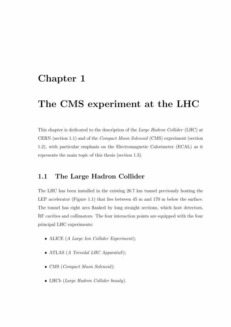
Figure 1.1: The LHC ring.
Being a particle-particle collider, there are two separate acceleration rings with
different magnetic field configuration. The beams are focused by 1232 dipole mag-
nets and 392 quadrupole magnets cooled down to 1.9 K by means of liquid Helium.
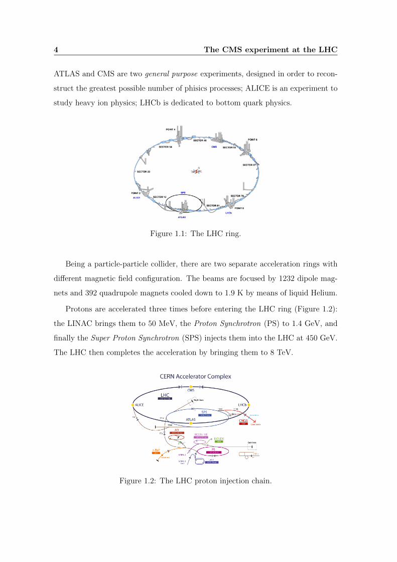
Protons are accelerated three times before entering the LHC ring (Figure 1.2):
the LINAC brings them to 50 MeV, the Proton Synchrotron (PS) to 1.4 GeV, and
finally the Super Proton Synchrotron (SPS) injects them into the LHC at 450 GeV.
The LHC then completes the acceleration by bringing them to 8 TeV.
Figure 1.2: The LHC proton injection chain.
The CMS experiment at the LHC 5
The number of physics events produced in pp collisions is N = σ · L, where σ
represents the cross section of the particular process and L the luminosity. The
LHC luminosity is defined as:
L =N2p · fBX · k
4π · σx · σy(1.1)
where Np is the number of protons per bunch, fBX the frequency of bunch crossing,
k the number of bunches, and σx and σy are the transverse spread of the bunches.
So, the high luminosity is obtained by a high frequency bunch crossing and a high
number of protons per bunch. The two proton beams contain each about 1368
bunches. The bunches, with a number of about 1.5 · 1011 protons each, have a
very small transverse spread (about 20 µm) and are about 7.5 cm long in the beam
direction. The bunches cross at the rate fBX = 20 MHz, i.e. there is a collision each
50 ns.
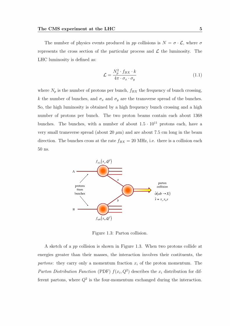
Figure 1.3: Parton collision.
A sketch of a pp collision is shown in Figure 1.3. When two protons collide at
energies greater than their masses, the interaction involves their costituents, the
partons : they carry only a momentum fraction xi of the proton momentum. The
Parton Distribution Function (PDF) f(xi, Q2) describes the xi distribution for dif-
ferent partons, where Q2 is the four-momentum exchanged during the interaction.
6 The CMS experiment at the LHC
The effective energy available in each parton collision is:
√s =√xaxbs (1.2)
where s = 4E2 is the centre of mass energy of the pp system (E is the energy of
the both protons), and xa and xb are the proton energy fractions carried by the two
interacting partons (a and b).
The cross section of a generic interaction pp→ X can be written as:
σ(pp→ X) =∑a,b
∫dxadxbfa(xa, Q
2)fb(xb, Q2)σ(ab→ X) (1.3)
where σ(ab→ X) is the cross section of the elementary interaction between partons
a and b at the centre of mass energy√s, and fa(xa, Q
2) and fb(xb, Q2) represent the
PDFs for the fraction xa and xb, respectively.
For a centre of mass energy of√s = 14 TeV at LHC, the total cross section is
estimated to be σ ' (100± 10) mb.
The inelastic collisions can be divided in two types:
• big distance parton collisions, in which a small Q2 is exchanged. These are
soft collisions where the majority of particles is produced at small momentum
pT and so it escapes from the detector along beam line. These events are the
so-called minimum bias events and they are the majority of the pp collisions.
• small distance parton collisions, in which a high Q2 is exchanged. In these in-
teractions high masses particles are produced with high momentum pT . These
events are the rare events. It needs a higher luminosity in order to have an
appreciable statistics of this kind of events.
Unfortunately, increasing luminosity means that many parton interactions overlap
in a same bunch crossing. In fact, given the instantaneous luminosity L and the
minimum bias cross section σmb, the average number of interactions in each bunch
The CMS experiment at the LHC 7
crossing (i.e. the number of the so-called pileup events) is given by:
µ =L · σmbfBX
(1.4)
At the nominal luminosity and for a minimum bias cross section of σmb = 80 mb, the
average number of inelastic collisions per bunch crossing is about 20, i.e. there are
109 interactions per second. This implies that the products of a selected interaction
can be confused with those of simultaneous interactions in the same bunch crossing.
The pileup effect can be reduced using a fine granularity detector with a good
time resolution. Moreover, since the maximum data storage rate sustainable by
the existing device technology is of O(100) Hz, a strong online event selection is
needed in order to reduce the event rate. The detector must also have a fast time
response (about 25 ns). In addition to this, the high flux of particles coming from
pp interactions implies that each component of the detector has to be radiation
resistant.
These are the general characteristics for a detector at LHC. The next section
will illustrate the specific features of the CMS experiment.
1.2 The Compact Muon Solenoid
The CMS detector [2] is a general purpose apparatus due to operate at LHC. The
detector requirements for CMS to meet the goal of the LHC physics programme are
the following:
• good muon identification and momentum resolution over a wide range of mo-
menta in the |η| ≤ 2.5, good dimuon mass resolution (' 1% at 100 GeV),
and the ability to determine unambiguously the charge of muons with p < 1
TeV/c;
• good charged-particle momentum resolution and reconstruction efficiency in
the inner tracker. Efficient triggering and offline tagging of τ ’s and b-jets,
8 The CMS experiment at the LHC
requiring pixel detectors close to the interaction region;
• good electromagnetic energy resolution, good diphoton and dielectron mass
resolution (' 1% at 100 GeV), wide geometric coverage, π0 rejection, and
efficient photon and lepton isolation at high luminosities;
• good missing-transverse-energy and dijet-mass resolution, requiring hadron
calorimeters with a large hermetic geometric coverage and with fine lateral
segmentation.
The design of CMS meets all these requirements. The main distinguishing features
of CMS are a high-field solenoid, a full-silicon-based inner tracking system, and a
homogenous scintillating-crystal-based electromagnetic calorimeter.
CMS has a cylindrical shape, symmetrical around the beam direction, with a
diameter of 14.6 m, a total length of 21.6 m, and weighs about 12500 tons. It
is divided into a central section, made of several layers coaxial to the beam axis
(the barrel), closed at its ends by two hermetic discs orthogonal to the beam (the
endcaps).
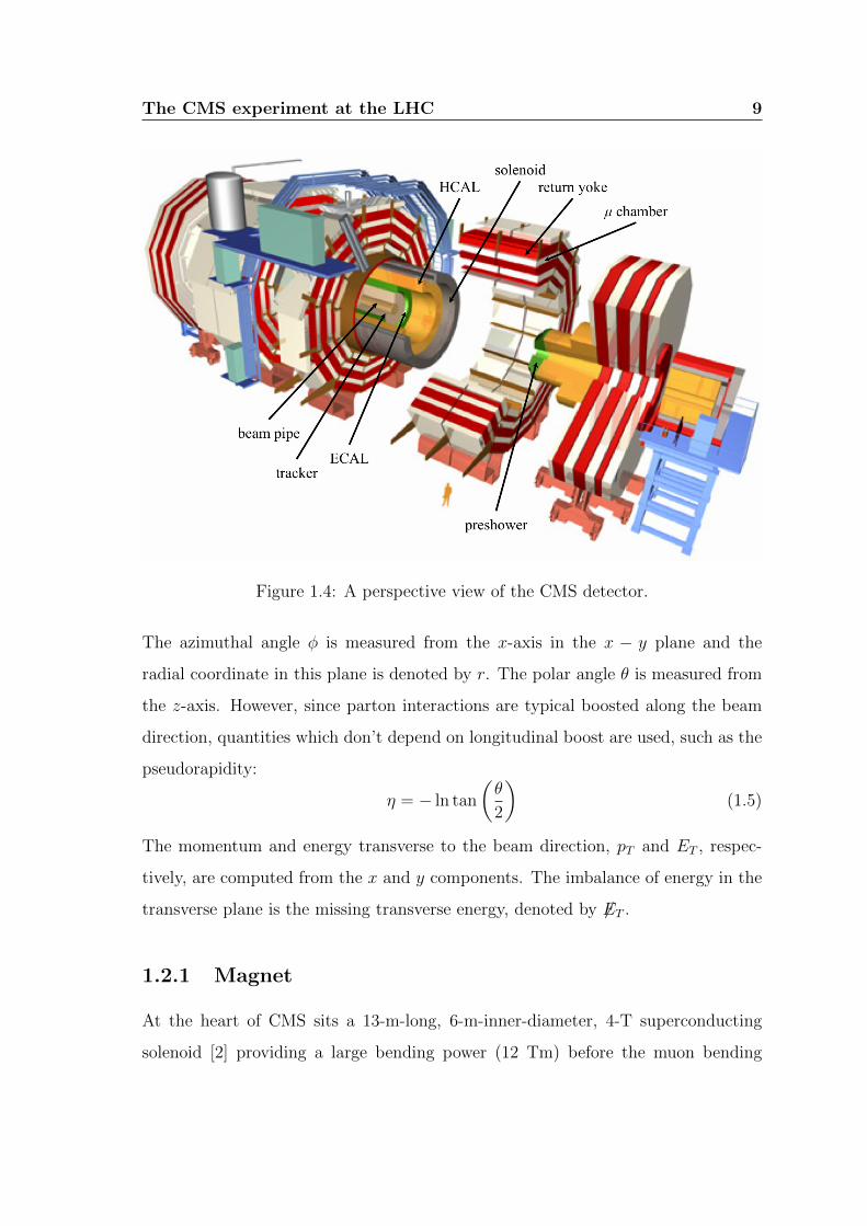
The overall layout of CMS is shown in Figure 1.4. Moving outside starting from
the beam position, it presents a silicon tracker, a crystal electromagnetic calorimeter,
a hadronic calorimeter, and the superconducting solenoidal magnet, in the return
yoke of which there are the muon drift chambers.
The coordinate system adopted by CMS has the origin centered at the nominal
collision point inside the detector:
• the x-axis pointing radially inward toward the center of the LHC;
• the y-axis points vertically upward;
• the z-axis points along the beam direction toward the Jura mountains from
LHC Point 5.
The CMS experiment at the LHC 9
Figure 1.4: A perspective view of the CMS detector.
The azimuthal angle φ is measured from the x-axis in the x − y plane and the
radial coordinate in this plane is denoted by r. The polar angle θ is measured from
the z-axis. However, since parton interactions are typical boosted along the beam
direction, quantities which don’t depend on longitudinal boost are used, such as the
pseudorapidity:
η = − ln tan
(θ
2
)(1.5)
The momentum and energy transverse to the beam direction, pT and ET , respec-
tively, are computed from the x and y components. The imbalance of energy in the
transverse plane is the missing transverse energy, denoted by 6ET .
1.2.1 Magnet
At the heart of CMS sits a 13-m-long, 6-m-inner-diameter, 4-T superconducting
solenoid [2] providing a large bending power (12 Tm) before the muon bending
10 The CMS experiment at the LHC
angle is measured by the muon system. The return field is large enough to saturate
1.5 m of iron. The bore of the magnet is large enough to accommodate the inner
tracker and the calorimetry.
1.2.2 Tracker
The main goal of the inner tracking [2] is to reconstruct isolated, high-pT electrons
and muons with efficiency greater than 95%, and tracks of particles within jets with
efficiency greater than 90%, within a pseudorapidity coverage of |η| < 2.5.
It surrounds the interaction vertex and has a length of 5.8 m and a diameter of
2.5 m. Since it is so close to the interaction region, the particle flux is such that
cause severe radiation damage to the detector. The main challenge in the design of
tracking system was to develop detector components able to operate in this harsh
environment for an expected lifetime of 10 years. In order to satisfy this requirement
the tracker is completely made of silicon and it constitutes the first example in high-
energy physics of an inner tracking system entirely based on this technology. By
considering the charged particle flux at high luminosity of the LHC, three regions
can be distinguished:
• the closest region to the interaction point where the particle flux is the highest
(' 107/s at r ' 10 cm), and there are pixel detectors. The pixel size is
100× 150 µm2;
• the intermediate region (20 cm < r < 55 cm), where the particle flux is low
enough to enable the use of silicon microstrip detectors with a minimum cell
size of 10 cm× 80 µm;
• the outermost region (r > 55 cm), where the particle flux has dropped suffi-
ciently to allow the adoption of larger-pitch silicon microstrips with a maxi-
mum cell size of 25 cm× 180 µm.
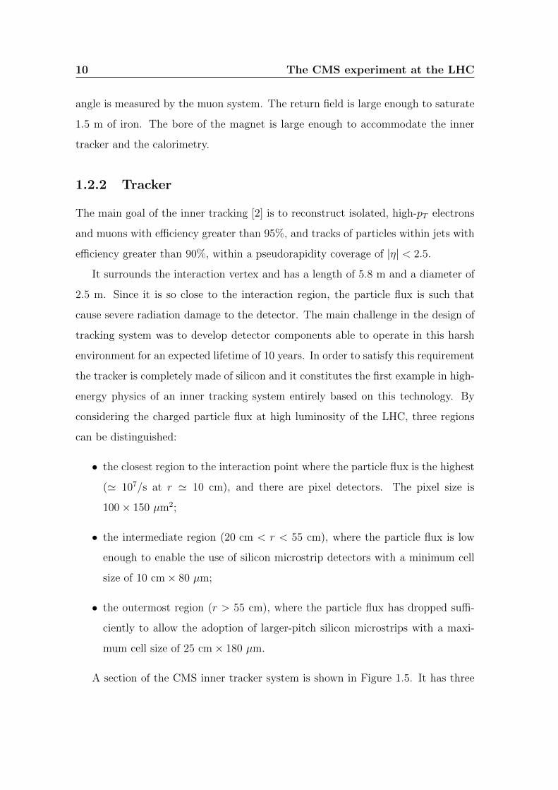
A section of the CMS inner tracker system is shown in Figure 1.5. It has three
The CMS experiment at the LHC 11
Figure 1.5: Longitudinal view of the inner tracker system.
cylindrical pixel layers in the barrel region, placed at radii 4.7 cm, 7.3 cm and 10.2
cm respectively, and two closing-discs, extending from 6 cm to 15 cm in radius, and
placed on each side at |z| = 34.5 cm and 46.5 cm. This design ensures that each
charged particle produced within |η| = 2.2 releases at least two hits in the pixel
detector.
The pixel layers are enveloped by a silicon microstrip detector. The barrel mi-
crostrip detector is divided into two regions: the inner and the outer barrel. The
inner barrel is made of four layers (the two innermost of which are double-sided),
and cover the depth 20 cm < r < 55 cm. The outer barrel counts six layers (the two
innermost double-sided) and reach up to the radius of 110 cm. In order to avoid that
particles hit the sensitive area at too small angles, the inner barrel is shorter than
the outer one, and three additional disc-shaped layers have been inserted between
the inner barrel and the endcaps. The endcap detector is made of nine layers of
discs, up to a maximum distance of |z| = 270 cm. The first, second and fifth layers
are double-sided.
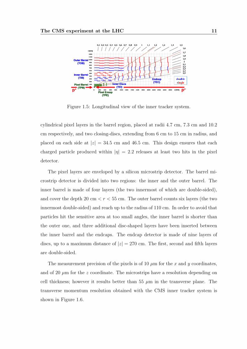
The measurement precision of the pixels is of 10 µm for the x and y coordinates,
and of 20 µm for the z coordinate. The microstrips have a resolution depending on
cell thickness; however it results better than 55 µm in the transverse plane. The
transverse momentum resolution obtained with the CMS inner tracker system is
shown in Figure 1.6.
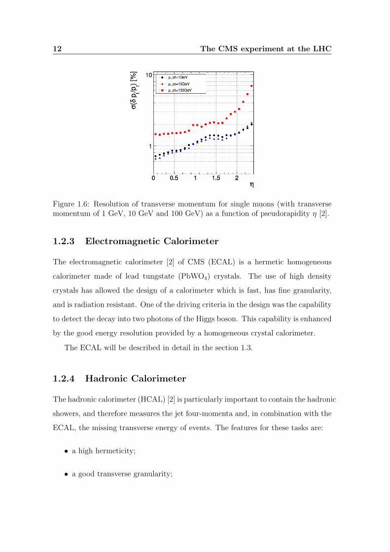
12 The CMS experiment at the LHC
Figure 1.6: Resolution of transverse momentum for single muons (with transversemomentum of 1 GeV, 10 GeV and 100 GeV) as a function of pseudorapidity η [2].
1.2.3 Electromagnetic Calorimeter
The electromagnetic calorimeter [2] of CMS (ECAL) is a hermetic homogeneous
calorimeter made of lead tungstate (PbWO4) crystals. The use of high density
crystals has allowed the design of a calorimeter which is fast, has fine granularity,
and is radiation resistant. One of the driving criteria in the design was the capability
to detect the decay into two photons of the Higgs boson. This capability is enhanced
by the good energy resolution provided by a homogeneous crystal calorimeter.
The ECAL will be described in detail in the section 1.3.
1.2.4 Hadronic Calorimeter
The hadronic calorimeter (HCAL) [2] is particularly important to contain the hadronic
showers, and therefore measures the jet four-momenta and, in combination with the
ECAL, the missing transverse energy of events. The features for these tasks are:
• a high hermeticity;
• a good transverse granularity;
The CMS experiment at the LHC 13
• a good energy resolution
• a sufficient longitudinal containment of the showers.
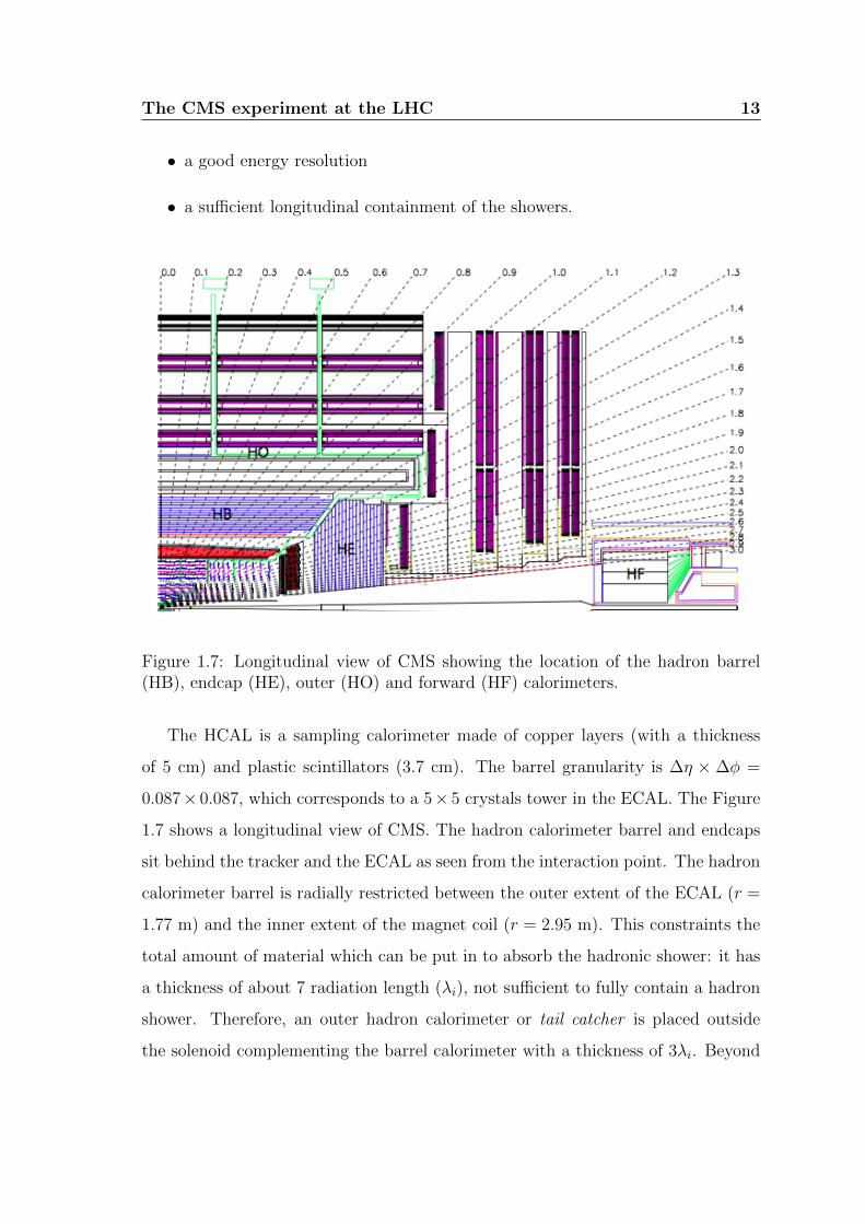
Figure 1.7: Longitudinal view of CMS showing the location of the hadron barrel(HB), endcap (HE), outer (HO) and forward (HF) calorimeters.
The HCAL is a sampling calorimeter made of copper layers (with a thickness
of 5 cm) and plastic scintillators (3.7 cm). The barrel granularity is ∆η × ∆φ =
0.087× 0.087, which corresponds to a 5× 5 crystals tower in the ECAL. The Figure
1.7 shows a longitudinal view of CMS. The hadron calorimeter barrel and endcaps
sit behind the tracker and the ECAL as seen from the interaction point. The hadron
calorimeter barrel is radially restricted between the outer extent of the ECAL (r =
1.77 m) and the inner extent of the magnet coil (r = 2.95 m). This constraints the
total amount of material which can be put in to absorb the hadronic shower: it has
a thickness of about 7 radiation length (λi), not sufficient to fully contain a hadron
shower. Therefore, an outer hadron calorimeter or tail catcher is placed outside
the solenoid complementing the barrel calorimeter with a thickness of 3λi. Beyond
14 The CMS experiment at the LHC
|η| = 3, the forward hadron calorimeters placed at 11.2 m from the interaction
vertex extend the pseudorapidity coverage down to |η| = 5.2 using a Cherenkov-
based, radiation-hard technology.
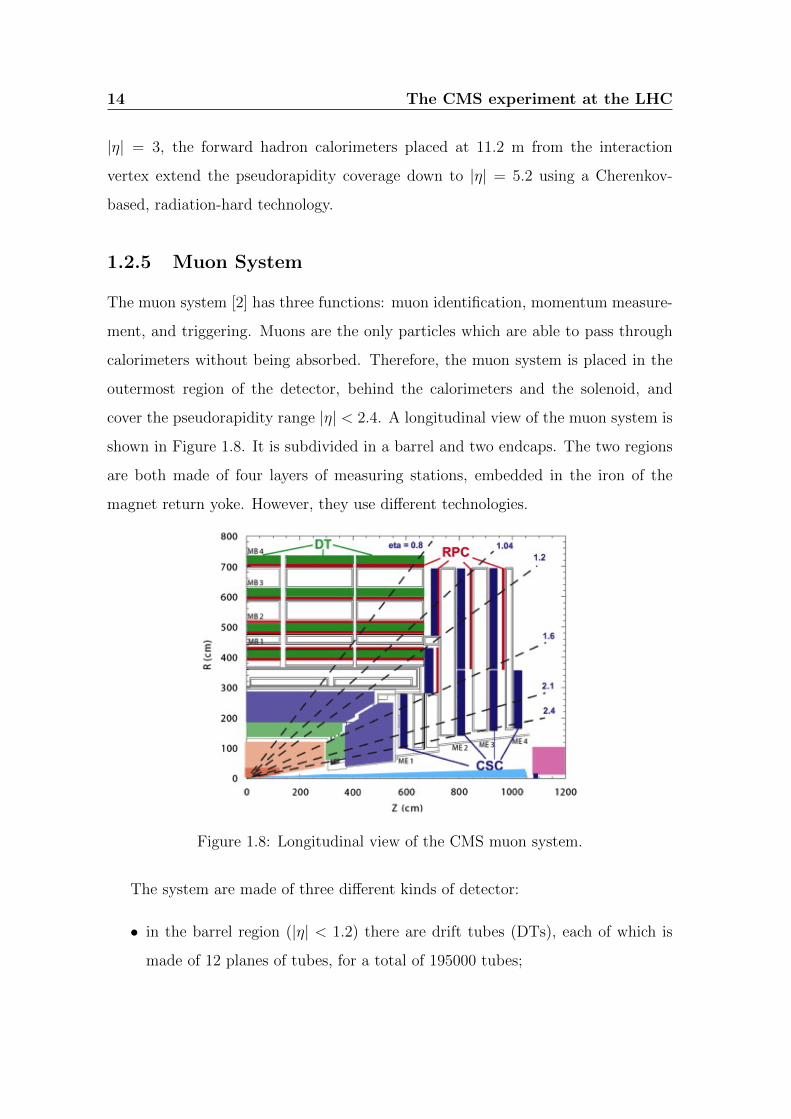
1.2.5 Muon System
The muon system [2] has three functions: muon identification, momentum measure-
ment, and triggering. Muons are the only particles which are able to pass through
calorimeters without being absorbed. Therefore, the muon system is placed in the
outermost region of the detector, behind the calorimeters and the solenoid, and
cover the pseudorapidity range |η| < 2.4. A longitudinal view of the muon system is
shown in Figure 1.8. It is subdivided in a barrel and two endcaps. The two regions
are both made of four layers of measuring stations, embedded in the iron of the
magnet return yoke. However, they use different technologies.
Figure 1.8: Longitudinal view of the CMS muon system.
The system are made of three different kinds of detector:
• in the barrel region (|η| < 1.2) there are drift tubes (DTs), each of which is
made of 12 planes of tubes, for a total of 195000 tubes;
The CMS experiment at the LHC 15
• in the endcaps (1.2 < |η| < 2.4) there are cathode strip chambers (CSCs),
organized in six-layer modules. They are multi-wire proportional chambers in
which the cathode plane has segmented into strips, and provide measurement
of precision in high magnetic fields;
• both in the barrel and in the endcaps resistive plate chambers (RPCs) have
been placed in order to supply a very fast trigger system. They are organized
in six barrel and four endcap stations, each of which is a parallel-plate chamber
with an excellent time resolution (3 ns).
The muon identification is provided by muon stations, while the measurement of
muon momentum is made by combining the information of the track in the muon
system with the information of the track in the inner tracking system, which has an
excellent resolution.
1.2.6 Trigger
At the present LHC luminosity the event rate is about 109 Hz, so the storage is
not possible for all pp collisions. However, not all the events are useful for the
CMS physics programme: in fact, the majority of the interactions is soft collisions.
Therefore, the aim of the trigger system [2] is to lower the rate of acquired events
to manageable levels (∼ 100 Hz), retaining at the same time most of the potentially
useful events.
The CMS trigger system consists of two consecutive steps: the first is a Level-1
Trigger (L1), and the second is a High-Level Trigger (HLT).
The L1 trigger reduces the rate of selected events to 50-100 kHz. It has to decide
whether taking or discarding data from a particular bunch crossing in 3.2 µs: if the
event is accepted, the data are moved to be processed by the HLT. Being the decision
time so short, then L1 can’t read data from the whole detector, but it employs only
the calorimetric and muon information, since the tracker algorithm is too slow for
this purpose. Therefore, the L1 trigger results organized in a Calorimetric Trigger
16 The CMS experiment at the LHC
and a Muon Trigger, whose information are transferred to the Global Trigger which
takes the final accept-rejection decision.
The HLT trigger is a software system and reduces the output rate to about
100 Hz. It employs various strategies, the guiding principle of which are a regional
reconstruction and a fast event veto. Regional reconstruction tries to avoid the
complete event reconstruction, which would take time, and focuses on the detector
regions close where L1 trigger has found an interesting activity. Fast event veto
means that uninteresting events are discarded as soon as possible, therefore freeing
the processing power for the next events in line.
1.3 The ECAL
The ECAL [3] is the subdetector dedicated to energy reconstruction of photons and
electrons. It plays a fundamental role in the Higgs search, especially in H → γγ
channel, and in the search for physics beyond the Standard Model. In this section,
the layout, the crystals and the energy resolution of the ECAL are described.
1.3.1 Layout and geometry
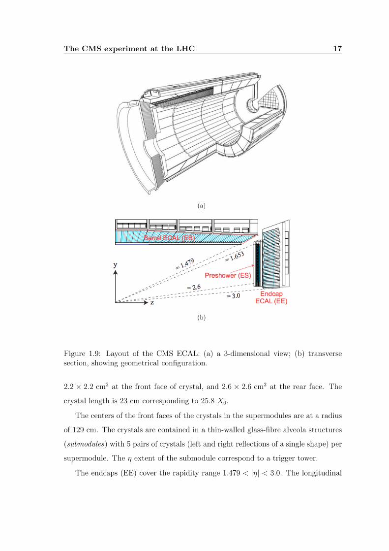
A 3-dimensional representation is shown in Figure 1.9(a). There are 36 identical
supermodules, 18 in each half barrel, each covering 20◦ in φ. The barrel is closed at
each end by an endcap. In front of most of the fiducial region of each endcap is a
preshower device. Figure 1.9(b) shows a transverse section through ECAL.
The barrel part of the ECAL (EB) covers the pseudorapidity range |η| < 1.479.
The barrel granularity is 360-fold in φ and (2 × 85)-fold in η, resulting in a total
of 61200 crystals. The truncated-pyramid shaped crystals are mounted in a quasi-
projective geometry so that their axes make a small angle (3◦) with respect to the
vector from the nominal interaction vertex, in both the φ and the η projections. The
crystal cross-section corresponds to approximately 0.0174× 0.0174 in η−φ plane or
The CMS experiment at the LHC 17
(a)
(b)
Figure 1.9: Layout of the CMS ECAL: (a) a 3-dimensional view; (b) transversesection, showing geometrical configuration.
2.2 × 2.2 cm2 at the front face of crystal, and 2.6 × 2.6 cm2 at the rear face. The
crystal length is 23 cm corresponding to 25.8 X0.
The centers of the front faces of the crystals in the supermodules are at a radius
of 129 cm. The crystals are contained in a thin-walled glass-fibre alveola structures
(submodules) with 5 pairs of crystals (left and right reflections of a single shape) per
supermodule. The η extent of the submodule correspond to a trigger tower.
The endcaps (EE) cover the rapidity range 1.479 < |η| < 3.0. The longitudinal
18 The CMS experiment at the LHC
distance between interaction point and the endcap envelop is 315.4 cm. The endcap
consists of identically shaped crystals grouped in mechanical units of 5× 5 crystals
(supercrystals or SCs) consisting of a carbon-fibre alveola structure. Each endcap is
divided into 2 halves or Dees. Each Dee comprises 3662 crystals. These are contained
in 138 standard SCs. The crystals and the SCs are arranged in a rectangular x− y
grid, with the crystals pointing at a focus 130 cm beyond the interaction point, so
that the off-pointing angle varies with η. The crystals have a rear face cross section
of about 3 × 3 cm2, a front face cross section of about 2.86 × 2.86 cm2 and length
of 22 cm (24.7 X0).
The preshower detector (ES) covers the pseudorapidity range 1.653 < |η| < 2.6.
Its principal aim is to distinguish photons and π0s. In fact, the latter rapidly decay
in two photons which are very close at high energy and so hardly separable. The ES
also helps the identification of electrons and photons with its superior granularity.
It is a sampling calorimeter with two layers: lead radiators initiate electromagnetic
showers from incoming photons/electrons, whilst silicon strip sensors placed after
each radiator measure the energy deposited and the transverse shower profiles.
1.3.2 Lead tungstate crystals
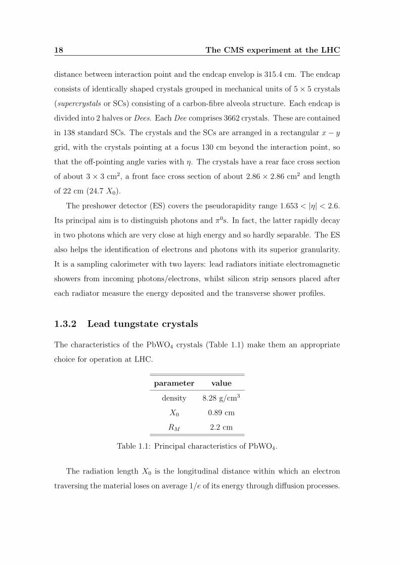
The characteristics of the PbWO4 crystals (Table 1.1) make them an appropriate
choice for operation at LHC.
parameter value
density 8.28 g/cm3
X0 0.89 cm
RM 2.2 cm
Table 1.1: Principal characteristics of PbWO4.
The radiation length X0 is the longitudinal distance within which an electron
traversing the material loses on average 1/e of its energy through diffusion processes.
The CMS experiment at the LHC 19
The ECAL has to ensure the complete restraint of the electromagnetic shower within
energy of TeV. For these energies the 98% of the longitudinal development is con-
tained in 25X0.
The Moliere radius RM is a quantity used to describe the transversal development
of an electromagnetic shower, and it is defined as:
RM =21.2 MeV ·X0
EC [MeV](1.6)
where EC represents the critic energy at which the ionization energy loss is equal to
Bremsstrahlung energy loss. The 90% of the shower is contained in a cylinder with
a radius of RM builded around the shower axis.
The choice of PbWO4 has been mainly driven by its short X0 and its small RM
which result in a compact calorimeter and a fine granularity necessary to distinguish
γ−π0 and for the angular resolution. Moreover, PbWO4 crystals have excellent hard-
radiation resistance and a scintillation decay time of the same order of magnitude
as the LHC bunch crossing time. This last property allow to collect the 85% of the
light in the interval between two successive pp intercations.
1.3.3 Photodetectors
The photodetectors need to be fast, radiation tolerant and be able to operate in the
longitudinal 4-T magnetic field. In addition, because of the small light yield of the
crystals, they should amplify and be insensitive to particles traversing them (nuclear
counter effect). The configuration of the magnetic field and the expected level of
radiation led to different choices: avalanche photodiodes (APDs) in the barrel, and
vacuum phototriodes (VPTs) in the endcaps. The lower quantum efficiency and
internal gain of the VPTs, compared to the APDs, are offset by their larger surface
coverage on the back face of the crystals.
20 The CMS experiment at the LHC
1.3.4 Energy resolution
The energy resolution of a homogeneous calorimeter can be expressed as a sum in
quadrature of three different terms:
σ(E)
E=
S√E⊕ N
E⊕ C (1.7)
where E is the energy expressed in GeV, and S, N and C represent the stochastic,
the noise and the constant terms, respectively. Different effects contribute to these
terms:
• the stochastic term S is a direct consequence of the Poissonian statistics asso-
ciated with the development of the electromagnetic shower in the calorimeter
and the successive recollection of the scintillation light. This term represents
the intrinsic resolution of an ideal calorimeter with infinite size and no response
deterioration due to instrumental effects. The original energy E0 of a particle
detected by a calorimeter is linearly related to the total track length Ltrack0 ,
defined as the sum of all the ionization tracks produced by all the charged par-
ticles in the electromagnetic shower. Since Ltrack0 is proportional to the number
of track segments in the shower and the shower development is a stochastic
process, the intrinsic resolution from purely statistical arguments is given by:
σ(E)
E∝√Ltrack0
Ltrack0
∝ 1√E0
(1.8)
For a real calorimeter, this term also absorbs the effects related to the shower
containment and the statistical fluctuations in the scintillation light recollec-
tion;
• the noise term N accounts for all the effects that can alter the measurements
of the energy deposit independently of the energy itself. It includes the elec-
tronic noise and the physical noise due to energy released by particles coming
The CMS experiment at the LHC 21
from multiple collision events. Electronic noise is mainly caused by the pho-
todetectors, that contribute basically via two components: one is proportional
to its capacitance, the other is connected to the fluctuations of the leakage
current;
• the constant term C dominates at high energy. Many different effects con-
tribute to this term: the stability of the operating conditions such as the
temperature and the high voltage of the photodetectors, the electromagnetic
shower containment and the presence of the dead material, the light collection
uniformity along the crystal axis, the radiation damage of PbWO4 crystals,
the intercalibration between the different channels.
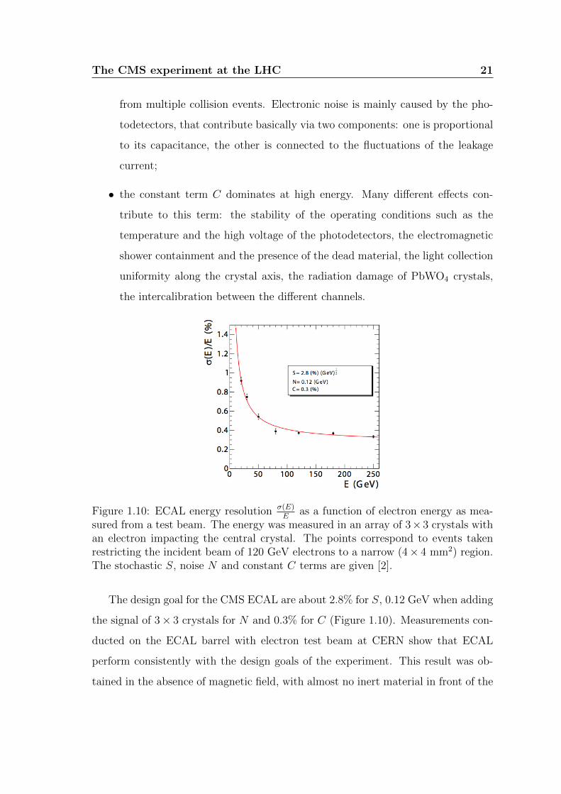
Figure 1.10: ECAL energy resolution σ(E)E
as a function of electron energy as mea-sured from a test beam. The energy was measured in an array of 3× 3 crystals withan electron impacting the central crystal. The points correspond to events takenrestricting the incident beam of 120 GeV electrons to a narrow (4× 4 mm2) region.The stochastic S, noise N and constant C terms are given [2].
The design goal for the CMS ECAL are about 2.8% for S, 0.12 GeV when adding
the signal of 3× 3 crystals for N and 0.3% for C (Figure 1.10). Measurements con-
ducted on the ECAL barrel with electron test beam at CERN show that ECAL
perform consistently with the design goals of the experiment. This result was ob-
tained in the absence of magnetic field, with almost no inert material in front of the
22 The CMS experiment at the LHC
calorimeter and with the beam aligned on the centers of crystals. The result is in
good agreement with the design-goal performance expected for a perfectly calibrated
detector.
The first 7 TeV LHC collisions recorded with the CMS detector have been used to
perform a channel-by-channel calibration of the ECAL [4]. Decays of π0 and η into
two photons as well as the azimuthal symmetry of the average energy deposition at a
given pseudorapidity are utilized to equalize the response of the individual channels
in barrel and endcaps. Based on an integrated luminosity of up to 250 nb−1, a
channel-by-channel in-situ calibration precision of 0.6% has been achieved in the
barrel ECAL in the pseudorapidity region |η| < 0.8. The energy scale of the ECAL
has been investigated and found to agree with the simulation to within 1% in the
barrel and 3% in the endcaps.
1.3.5 Photon reconstruction
Photon showers deposit their energy in several crystals in the ECAL. Approximately
94% of the incident energy of a single unconverted photon is contained in 3 × 3
crystals, and 97% in 5 × 5 crystals. Summing the energy measured in such fixed
arrays gives the best performance for unconverted photons. The presence in CMS
of material in front of the calorimeter results in photon conversions. Unconverted
and converted photons are distinguished from each other by means of the variable
R9 = E9Eγ
, where E9 is the energy collected by a 3 × 3 crystals array, and Eγ is
the photon energy. In fact, unconverted photons or photons converted very close
to the ECAL have values of R9 towards unity, whereas lower values of R9 describe
an increase of the energy spread. Because of the strong magnetic field the energy
reaching the calorimeter is spread in φ. The spread energy is clustered by building a
cluster of clusters, a so-called supercluster, which is extended in φ. The supercluster
position (i.e. the impact point of the photon) is obtained by calculating the energy-
weighted mean position of the crystals in the cluster.
The CMS experiment at the LHC 23
The triggering photons selected by the HLT provide the starting point for offline
reconstruction and selection of prompt photons. These selected photons already
have transverse energy above the HLT selection thresholds and have passed the
isolation criteria of the L1 and HLT selection (for details about photon trigger, see
section 10.2 of [3]).
Fake photons are due to electromagnetic component of a jet, mainly due to
neutral pions. To reject such a background, isolation criteria are applied, both at
trigger and analysis level. They are based on the presence of additional particles
in a cone around the reconstructed ECAL cluster. Charged pions and kaons can
be detected with the tracker or in the HCAL. Neutral pions and other particles
decaying into photons can be detected in the ECAL.
The size of the veto cones is optimized to take into account the energy spread in
the calorimeter due to showering and magnetic field.
The basic isolation variables considered are based on charged tracks recon-
structed in the tracker, electromagnetic deposits observed in the ECAL, and hadronic
energy deposits in the HCAL. These variables are combined to have a global isolation
information.
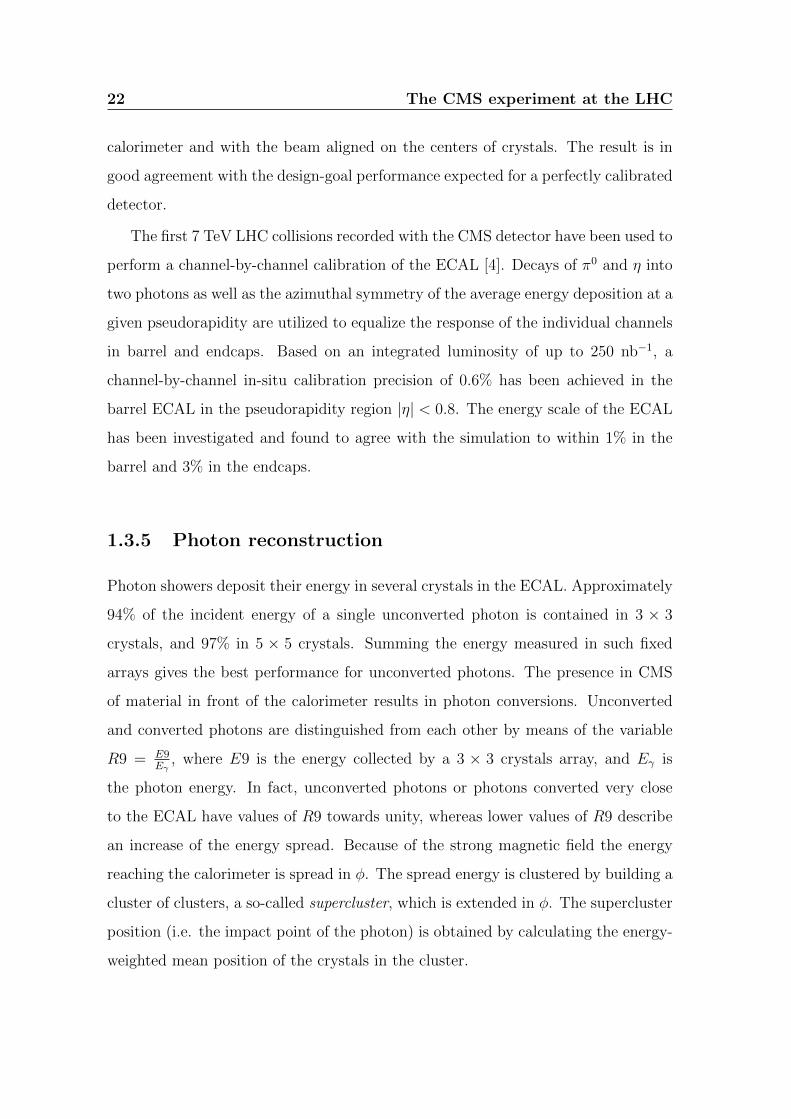
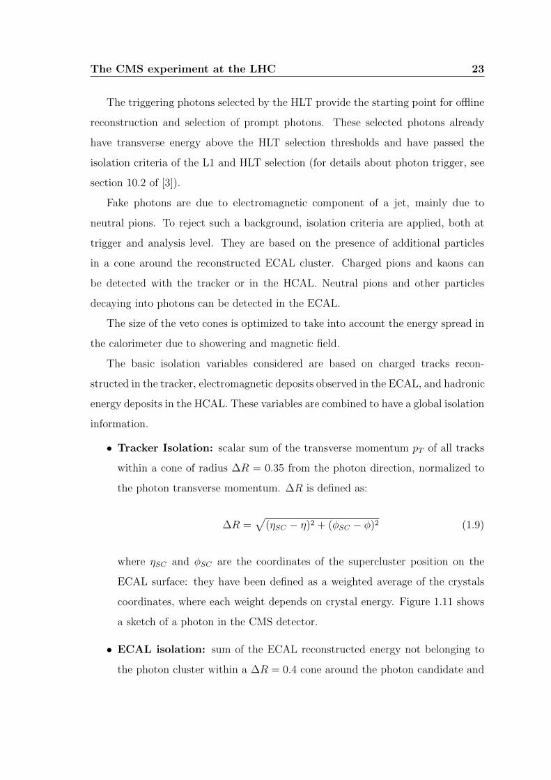
• Tracker Isolation: scalar sum of the transverse momentum pT of all tracks
within a cone of radius ∆R = 0.35 from the photon direction, normalized to
the photon transverse momentum. ∆R is defined as:
∆R =√
(ηSC − η)2 + (φSC − φ)2 (1.9)
where ηSC and φSC are the coordinates of the supercluster position on the
ECAL surface: they have been defined as a weighted average of the crystals
coordinates, where each weight depends on crystal energy. Figure 1.11 shows
a sketch of a photon in the CMS detector.
• ECAL isolation: sum of the ECAL reconstructed energy not belonging to
the photon cluster within a ∆R = 0.4 cone around the photon candidate and
24 The CMS experiment at the LHC
normalized to the photon energy.
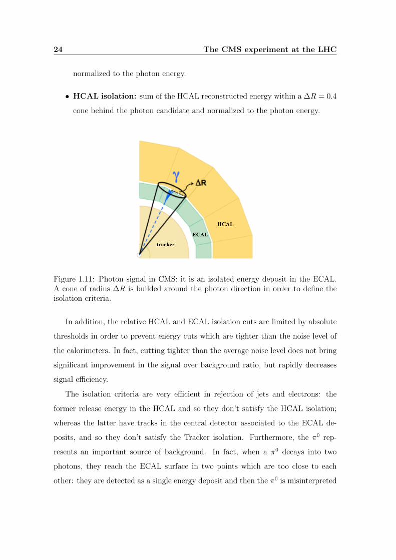
• HCAL isolation: sum of the HCAL reconstructed energy within a ∆R = 0.4
cone behind the photon candidate and normalized to the photon energy.
Figure 1.11: Photon signal in CMS: it is an isolated energy deposit in the ECAL.A cone of radius ∆R is builded around the photon direction in order to define theisolation criteria.
In addition, the relative HCAL and ECAL isolation cuts are limited by absolute
thresholds in order to prevent energy cuts which are tighter than the noise level of
the calorimeters. In fact, cutting tighter than the average noise level does not bring
significant improvement in the signal over background ratio, but rapidly decreases
signal efficiency.
The isolation criteria are very efficient in rejection of jets and electrons: the
former release energy in the HCAL and so they don’t satisfy the HCAL isolation;
whereas the latter have tracks in the central detector associated to the ECAL de-
posits, and so they don’t satisfy the Tracker isolation. Furthermore, the π0 rep-
resents an important source of background. In fact, when a π0 decays into two
photons, they reach the ECAL surface in two points which are too close to each
other: they are detected as a single energy deposit and then the π0 is misinterpreted
The CMS experiment at the LHC 25
as a photon of the same energy. In order to distinguish between photons and neutral
pions, the isolation criteria are not sufficient: the γ − π0 discrimination algorithm
exploits the differences on the shape of γ and π0 deposits, which can be described
by the so-called cluster shape variables, defined later.
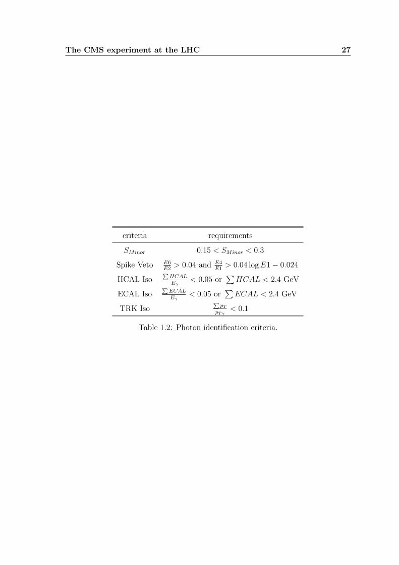
A photon candidate has to satisfy a set of requirements (photonID) summarized
in Table 1.2. In addition to the tracker, ECAL and HCAL isolation, there are
specific requirements:
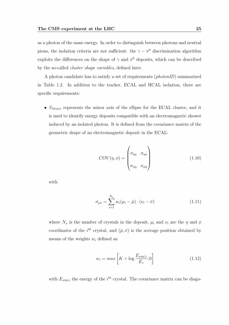
• SMinor represents the minor axis of the ellipse for the ECAL cluster, and it
is used to identify energy deposits compatible with an electromagnetic shower
induced by an isolated photon. It is defined from the covariance matrix of the
geometric shape of an electromagnetic deposit in the ECAL:
COV (η, φ) =
σηη σηφ
σφη σφφ
(1.10)
with
σµν =Nx∑i=1
wi(µi − µ) · (νi − ν) (1.11)
where Nx is the number of crystals in the deposit, µi and νi are the η and φ
coordinates of the ith crystal, and (µ, ν) is the average position obtained by
means of the weights wi defined as:
wi = max
[K + log
Extal,iEγ
; 0
](1.12)
with Extal,i the energy of the ith crystal. The covariance matrix can be diago-
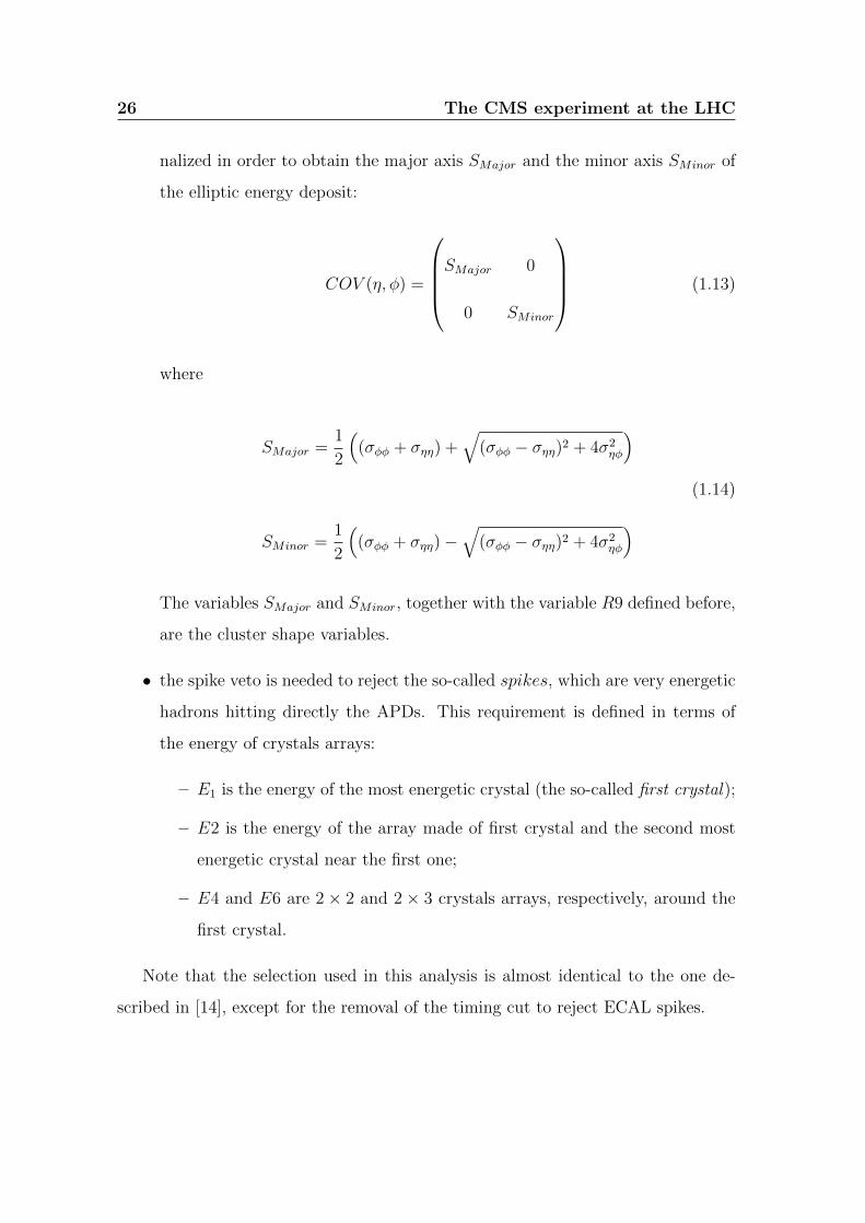
26 The CMS experiment at the LHC
nalized in order to obtain the major axis SMajor and the minor axis SMinor of
the elliptic energy deposit:
COV (η, φ) =
SMajor 0
0 SMinor
(1.13)
where
SMajor =1
2
((σφφ + σηη) +
√(σφφ − σηη)2 + 4σ2
ηφ
)
SMinor =1
2
((σφφ + σηη)−
√(σφφ − σηη)2 + 4σ2
ηφ
)(1.14)
The variables SMajor and SMinor, together with the variable R9 defined before,
are the cluster shape variables.
• the spike veto is needed to reject the so-called spikes, which are very energetic
hadrons hitting directly the APDs. This requirement is defined in terms of
the energy of crystals arrays:
– E1 is the energy of the most energetic crystal (the so-called first crystal);
– E2 is the energy of the array made of first crystal and the second most
energetic crystal near the first one;
– E4 and E6 are 2 × 2 and 2 × 3 crystals arrays, respectively, around the
first crystal.
Note that the selection used in this analysis is almost identical to the one de-
scribed in [14], except for the removal of the timing cut to reject ECAL spikes.
The CMS experiment at the LHC 27
criteria requirements
SMinor 0.15 < SMinor < 0.3
Spike Veto E6E2
> 0.04 and E4E1
> 0.04 logE1− 0.024
HCAL Iso∑HCALEγ
< 0.05 or∑HCAL < 2.4 GeV
ECAL Iso∑ECALEγ
< 0.05 or∑ECAL < 2.4 GeV
TRK Iso∑pT
pTγ< 0.1
Table 1.2: Photon identification criteria.

Chapter 2
Time reconstruction in the ECAL
The combination of the scintillation timescale of the PbWO4, the electronic pulse
shaping and the sampling rate allow for an excellent time resolution to be obtained
with the ECAL. This is important in CMS in many respects. The better the pre-
cision of time measurement and synchronization, the larger the rejection of back-
grounds with a broad time distribution. Such backgrounds are cosmic rays, beam
halo muons, electronic noise, and out-of-time proton-proton interactions. Precise
time measurement also makes it possible to identify particles predicted by different
models beyond the Standard Model. Slow heavy charged R-hadrons, which travel
through the calorimeter and interact before decaying, and photons from the decay of
long-lived new particles reach the calorimeter out-of-time with respect to particles
traveling at the speed of light from the interaction point. As an example, to iden-
tify neutralinos decaying into photons with decay lengths comparable to the ECAL
radial size, a time measurement resolution better than 1 ns is necessary. To achieve
these goals the time measurement performance both at low energy (1 GeV or less)
and high energy (several tens of GeV for showering photons) becomes relevant. In
addition, amplitude reconstruction of ECAL energy deposits benefits greatly if all
ECAL channels are synchronized within 1 ns. Previous experiments have shown that
it is possible to measure time with electromagnetic calorimeters with a resolution
better than 1 ns [5].
30 Time reconstruction in the ECAL
In this chapter a description of the time extraction with a single crystal (section
2.1) and a study of the time reconstruction for high transverse momentum photons
(section 2.2) will be given.
2.1 Time reconstruction study with data from the
test beam
2.1.1 Time extraction with ECAL crystals
When a photon hits a PbWO4 crystal, it releases an energy deposit (called rechit).
The resulting scintillation light is collected by the photodetectors (APDs and VPTs),
and their signal is amplified and shaped by the front-end electronics. The pulse is
then digitized at 40 MHz by an analog-to-digital converter (ADC), and finally the
energy measured in GeV is obtained from the ADC count.
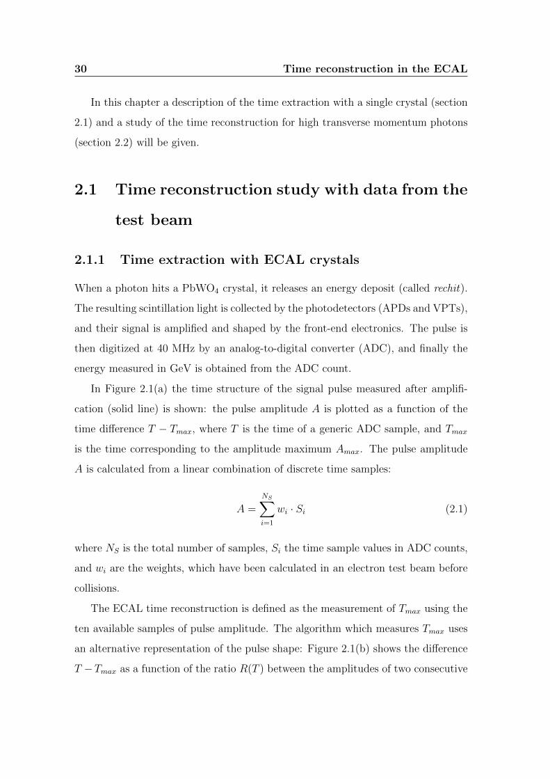
In Figure 2.1(a) the time structure of the signal pulse measured after amplifi-
cation (solid line) is shown: the pulse amplitude A is plotted as a function of the
time difference T − Tmax, where T is the time of a generic ADC sample, and Tmax
is the time corresponding to the amplitude maximum Amax. The pulse amplitude
A is calculated from a linear combination of discrete time samples:
A =
NS∑i=1
wi · Si (2.1)
where NS is the total number of samples, Si the time sample values in ADC counts,
and wi are the weights, which have been calculated in an electron test beam before
collisions.
The ECAL time reconstruction is defined as the measurement of Tmax using the
ten available samples of pulse amplitude. The algorithm which measures Tmax uses
an alternative representation of the pulse shape: Figure 2.1(b) shows the difference
T −Tmax as a function of the ratio R(T ) between the amplitudes of two consecutive
Time reconstruction in the ECAL 31
digitizations, defined as:
R(T ) =A(T )
A(T + 25 ns)(2.2)
This signal representation is independent of Amax and is described by a simple
polynomial parameterization.
(a) (b)
Figure 2.1: (a) Typical pulse shape measured in the ECAL as a function of thedifference T − Tmax. The dots indicate ten discrete samples of the pulse, from asingle event, with pedestal subtracted and normalized to Amax. The solid line is theaverage pulse shape. (b) T − Tmax as a function of R(T ) [5].
Each pair of consecutive samples gives a measurement of the ratio Ri = Ai/Ai+1,
from which an estimate of Tmax,i = Ti − T (Ri) can be extracted with its relative
uncertainty σi, where Ti is the time when the sample i is taken, and T (Ri) is the
time corresponding to the amplitude Ri as given by the parametrization in Figure
2.1(b). The time of the pulse maximum Tmax and its error are then evaluated from
the weighted average of the estimated Tmax,i:
Tmax =
∑i
Tmax,iσ2i∑
i
1
σ2i
,1
σ2Tmax
=∑i
1
σ2i
(2.3)
32 Time reconstruction in the ECAL
2.1.2 Time measurement resolution
The time resolution can be expressed as the sum in quadrature of three terms:
σ2(t) =
(NσnA
)2
+
(S√A
)2
+ C2 (2.4)
where A is the measured amplitude, σn is related to the electronics noise, and N , S
and C represent the noise, stochastic, and constant term, respectively. Monte Carlo
simulation studies give N = 33 ns, when the electronic noise σn is∼ 0.042 GeV in the
barrel and ∼ 0.14 GeV in the endcaps. The stochastic term comes from fluctuations
in photon collection times, associated with the finite time of scintillation emission.
It is estimated to be negligible. The constant term takes into account effects due
to the point of shower initiation within the crystal, and systematic effects in the
time extraction, such as those due to small differences in pulse shape for different
channels.
The first determination of the time resolution has been obtained with test beam
data, prior to collisions. The methods used the distribution of the time difference
between adjacent crystals that share energy from the same electromagnetic shower.
This approach is less sensitive to the term C, since effects due to synchronization do
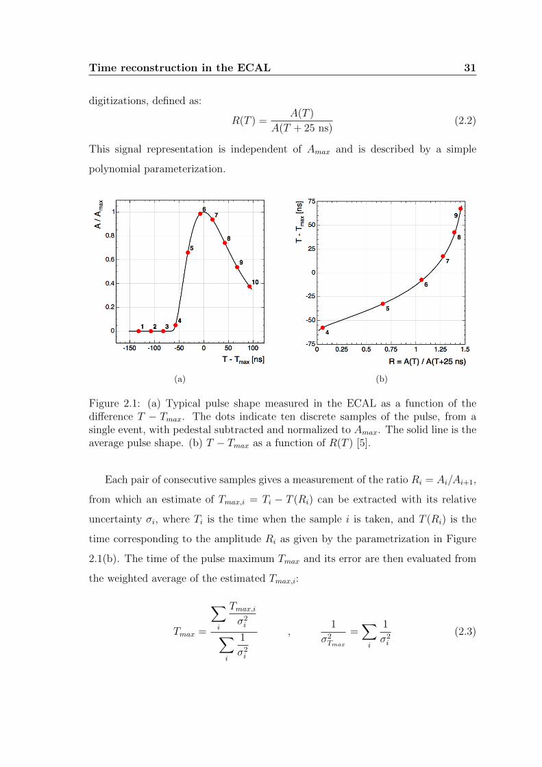
not affect the spread but only the average of the time difference. Then the spread
in time difference between adjacent crystals is parameterized as:
σ2(t1 − t2) =
(N
Aeff/σn
)2
+ 2C2 (2.5)
where Aeff = E1E2/√E2
1 + E22 with t1,2 and E1,2 corresponding to the times and
energies measured in the two crystals, and C is the residual contribution from the
constant terms. The extracted width is shown in Figure 2.2 as a function of the
variable Aeff/σn. The fitted noise term corresponds to N = (35.1 ± 0.2) ns, and C
is very small: C = (0.020 ± 0.004) ns. Note that the constant term C takes into
account of the error due to the so-called intercalibration between crystals, σintercalib.
Time reconstruction in the ECAL 33
Figure 2.2: Spread of the time difference between two neighboring crystals as afunction of the variable Aeff/σn for the electron test beam. The equivalent single-crystal energy scales for barrel (EB) and endcaps (EE) are overlaid in the plot [5].
As shown, for large values of Aeff/σn, which correspond to an energy greater than
10 GeV in the EB, σ(t) is less than 100 ps, demonstrating that, with a carefully
calibrated detector, it is possible to reach a time resolution better than 100 ps for
large energy deposits (E > 10− 20 GeV in the EB).
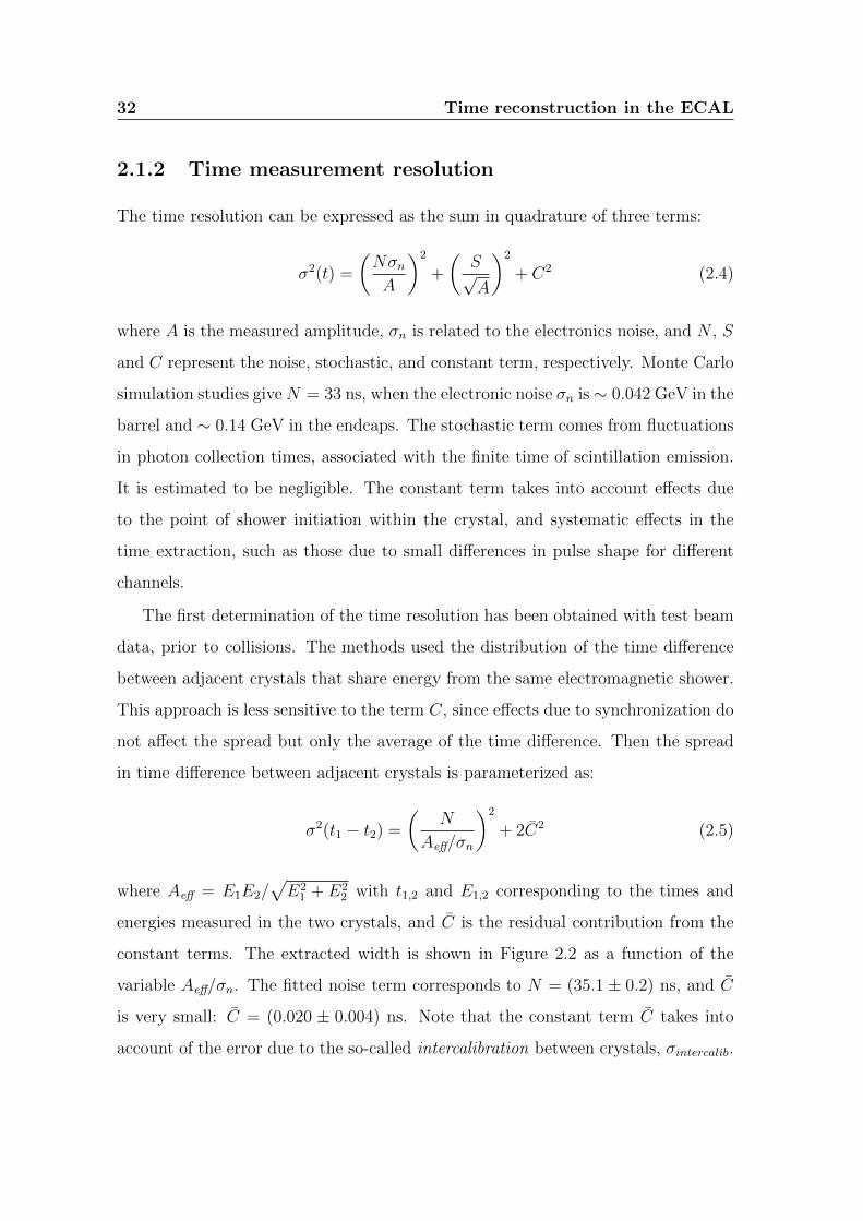
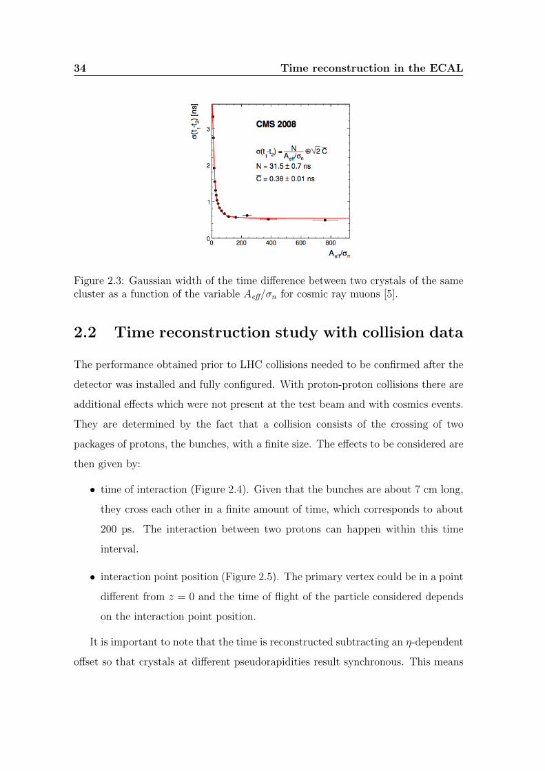
The time resolution is also determined with a sample of cosmic ray muons col-
lected during summer 2008, when the ECAL was already inserted into its final
position in CMS. The approach to extract the resolution is similar to that made at
the test beam, but in this case the crystal with the maximum amplitude is compared
with the other crystals in the cluster. Since different pairs of crystals are used, a
constant term comparable with the systematic uncertainty of the synchronization
(section 4 of [5]) is expected. The spread of the time difference between crystals of
the same cluster as a function of Aeff/σn is shown in Figure 2.3. The noise term
is found to be N = (31.5 ± 0.7) ns and is very similar to that obtained from test
beam data. The constant term is C = (0.38± 0.10) ns, which is consistent with the
expected systematic uncertainty from synchronization.
34 Time reconstruction in the ECAL
Figure 2.3: Gaussian width of the time difference between two crystals of the samecluster as a function of the variable Aeff/σn for cosmic ray muons [5].
2.2 Time reconstruction study with collision data
The performance obtained prior to LHC collisions needed to be confirmed after the
detector was installed and fully configured. With proton-proton collisions there are
additional effects which were not present at the test beam and with cosmics events.
They are determined by the fact that a collision consists of the crossing of two
packages of protons, the bunches, with a finite size. The effects to be considered are
then given by:
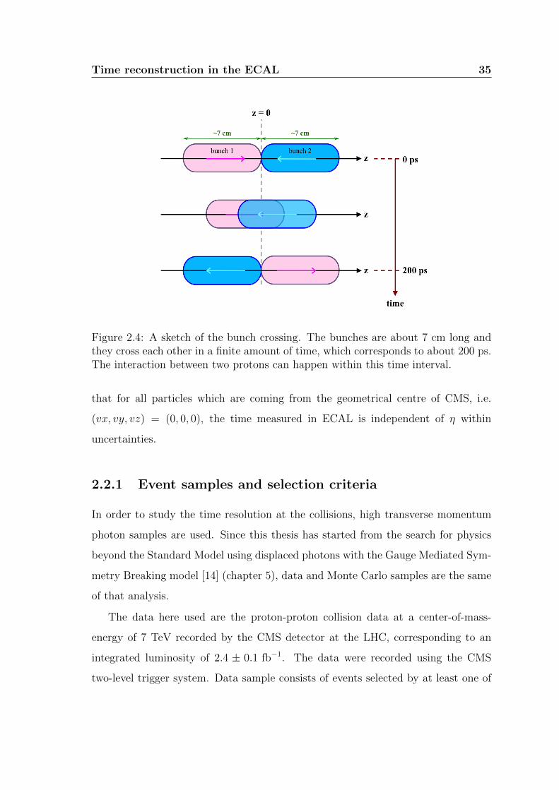
• time of interaction (Figure 2.4). Given that the bunches are about 7 cm long,
they cross each other in a finite amount of time, which corresponds to about
200 ps. The interaction between two protons can happen within this time
interval.
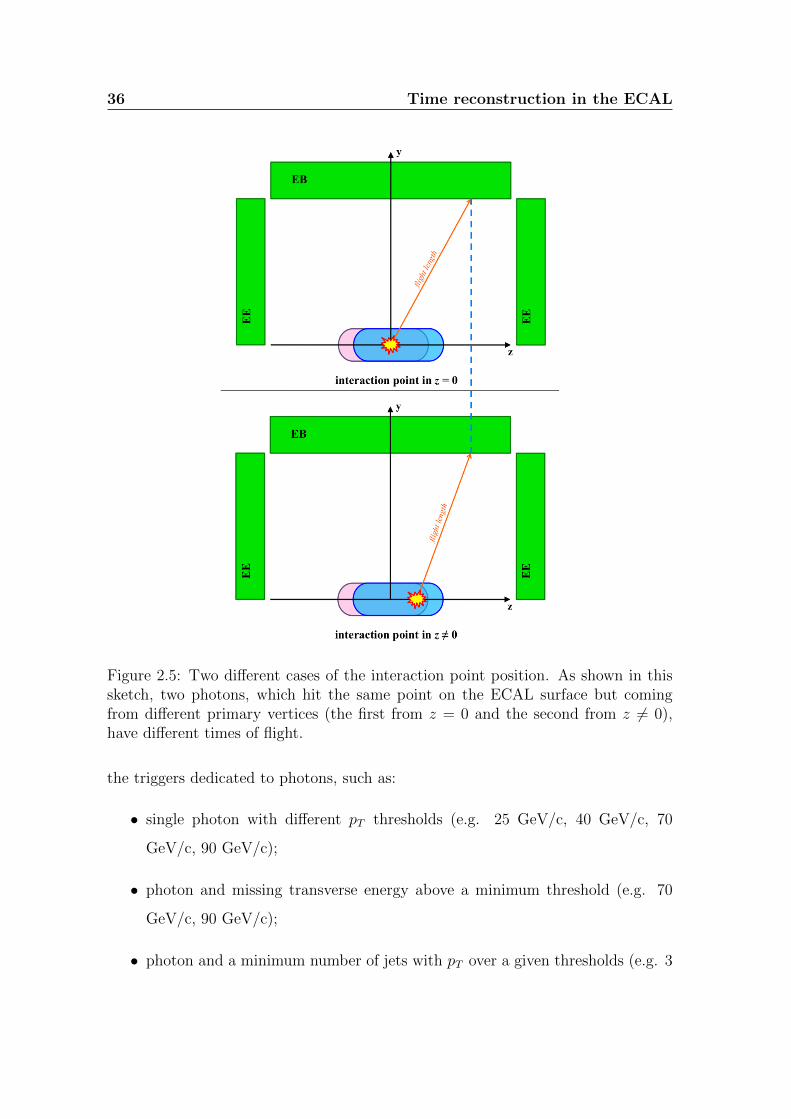
• interaction point position (Figure 2.5). The primary vertex could be in a point
different from z = 0 and the time of flight of the particle considered depends
on the interaction point position.
It is important to note that the time is reconstructed subtracting an η-dependent
offset so that crystals at different pseudorapidities result synchronous. This means
Time reconstruction in the ECAL 35
Figure 2.4: A sketch of the bunch crossing. The bunches are about 7 cm long andthey cross each other in a finite amount of time, which corresponds to about 200 ps.The interaction between two protons can happen within this time interval.
that for all particles which are coming from the geometrical centre of CMS, i.e.
(vx, vy, vz) = (0, 0, 0), the time measured in ECAL is independent of η within
uncertainties.
2.2.1 Event samples and selection criteria
In order to study the time resolution at the collisions, high transverse momentum
photon samples are used. Since this thesis has started from the search for physics
beyond the Standard Model using displaced photons with the Gauge Mediated Sym-
metry Breaking model [14] (chapter 5), data and Monte Carlo samples are the same
of that analysis.
The data here used are the proton-proton collision data at a center-of-mass-
energy of 7 TeV recorded by the CMS detector at the LHC, corresponding to an
integrated luminosity of 2.4 ± 0.1 fb−1. The data were recorded using the CMS
two-level trigger system. Data sample consists of events selected by at least one of
36 Time reconstruction in the ECAL
Figure 2.5: Two different cases of the interaction point position. As shown in thissketch, two photons, which hit the same point on the ECAL surface but comingfrom different primary vertices (the first from z = 0 and the second from z 6= 0),have different times of flight.
the triggers dedicated to photons, such as:
• single photon with different pT thresholds (e.g. 25 GeV/c, 40 GeV/c, 70
GeV/c, 90 GeV/c);
• photon and missing transverse energy above a minimum threshold (e.g. 70
GeV/c, 90 GeV/c);
• photon and a minimum number of jets with pT over a given thresholds (e.g. 3
Time reconstruction in the ECAL 37
jets with pT > 25 GeV/c);
• double photons with a pT threshold at 20 GeV/c on single photon and a
minimum value of the invariant mass (e.g. 60 GeV/c, 80 GeV/c).
Note that the different pT thresholds are motivated by the fact that during the data
taking the triggers with the lower thresholds are prescaled1 due to the increasing
luminosity.
Moreover, in the trigger selection, isolation criteria, less restrictive than those
required in the offline selection, are applied to photons.
There is a non-negligible probability that several collisions may occur in a single
bunch crossing due to the high instantaneous luminosities at the LHC. The average
number of multiple interaction vertices (pileup) for this data sample is about 8 in
each bunch crossing.
The Monte Carlo samples are simulated with pythia 6.4.22 [6] or MadGraph
5 [7] with the CTEQ6L1 [8] parton distribution functions (PDFs). The response of
the CMS detector is simulated using the Geant4 package [9]. The SUSY GMSB
signal production follows the SPS8 [22] proposal, where the free parameters are the
SUSY breaking scale Λ and the average proper decay length cτ of the neutralino.
The χ01 mass explored is in the range of 140 to 260 GeV (corresponding to Λ values
from 100 to 180 TeV), with proper decay length cτ = 1 mm, i.e. the point to the
primary vertex. More details will be provided in chapter 5.
Events satisfying trigger requirements have to pass additional selection criteria
based on vertexing: events with a good vertex are selected, i.e. there is a primary
vertex with at least 4 associated tracks (vndof ≥ 4), whose position is less than 2
cm from the centre of CMS in the direction transverse to the beam (√vx2 + vy2 < 2
cm) and 24 cm in the direction along the beam (|vz| < 24 cm), where vx, vy and
vz indicate the x, y and z coordinates of the primary vertex, respectively. Then,
1If the rate of a given trigger is too high, due to the luminosity increase, a prescale factor isfixed (e.g. 10: this means that for every 10 events, only one is stored).
38 Time reconstruction in the ECAL
the most energetic photon, satisfying the isolation criteria listed in Table 1.2, have
to pass the criteria pTγ ≥ 20 GeV/c and ηγ ≤ 2.52.
criteria requirements
good vertex vndof ≥ 4 ,√vx2 + vy2 < 2 cm , |vz| < 24 cm
|ηγ| ≤ 2.5
pTγ ≥ 20 GeV/c
Table 2.1: One photon events selection criteria.
2.2.2 Reconstruction of time of impact for photons
The time resolution of single crystal, σxtal,i, is studied. Note that σxtal,i, as detailed
in section 2.1.2, is the squared sum of two terms: the noise term, which is inversely
proportional to the energy of the crystal Extal,i, and the constant term, which takes
into account of the intercalibration error σintercal:
σ2xtal,i =
(N
σnExtal,i
)2
+ σ2intercal (2.6)
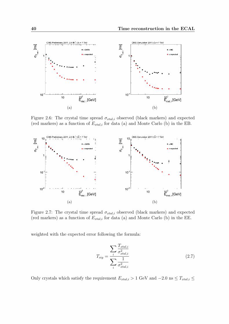
From the electron test beam [5] the coefficients N and σn correspond to N = 35.1
ns and σn = 0.042 GeV in the EB and σn = 0.14 GeV in the EE. The validity of
this parametrization has been verified using the spread of the time distribution of
the selected photons as a function of the energy of the crystal. A 2-dimensional
histogram of the time of the single crystal, Txatl,i, versus its energy Extal,i is plotted
separately for EB and EE. The time spread is extracted in bins of Extal,i via a
Gaussian fit as shown in Figures 2.6 and 2.7 (black markers). The resulting fitted
values are then compared with the expected values [5] (red markers). As shown,
there is a disagreement. For Monte Carlo, a full compatibility was not expected,
2Note that the gaps between barrel and endcaps (i.e. the ranges −1.566 ≤ η ≤ −1.4442 and1.4442 ≤ η ≤ 1.566) are excluded from the analysis, because some cluster energy can be lost innon-sensitive parts of the detector.
Time reconstruction in the ECAL 39
while on data the difference is due to hardware configuration compared to test beam,
which results in a different detector noise. The noise term which best represents the
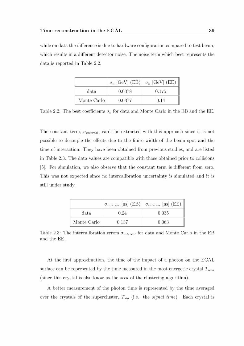
data is reported in Table 2.2.
σn [GeV] (EB) σn [GeV] (EE)
data 0.0378 0.175
Monte Carlo 0.0377 0.14
Table 2.2: The best coefficients σn for data and Monte Carlo in the EB and the EE.
The constant term, σintercal, can’t be extracted with this approach since it is not
possible to decouple the effects due to the finite width of the beam spot and the
time of interaction. They have been obtained from previous studies, and are listed
in Table 2.3. The data values are compatible with those obtained prior to collisions
[5]. For simulation, we also observe that the constant term is different from zero.
This was not expected since no intercalibration uncertainty is simulated and it is
still under study.
σintercal [ns] (EB) σintercal [ns] (EE)
data 0.24 0.035
Monte Carlo 0.137 0.063
Table 2.3: The intercalibration errors σintercal for data and Monte Carlo in the EBand the EE.
At the first approximation, the time of the impact of a photon on the ECAL
surface can be represented by the time measured in the most energetic crystal Tseed
(since this crystal is also know as the seed of the clustering algorithm).
A better measurement of the photon time is represented by the time averaged
over the crystals of the supercluster, Tsig (i.e. the signal time). Each crystal is
40 Time reconstruction in the ECAL
(a) (b)
Figure 2.6: The crystal time spread σxtal,i observed (black markers) and expected(red markers) as a function of Extal,i for data (a) and Monte Carlo (b) in the EB.
(a) (b)
Figure 2.7: The crystal time spread σxtal,i observed (black markers) and expected(red markers) as a function of Extal,i for data (a) and Monte Carlo (b) in the EE.
weighted with the expected error following the formula:
Tsig =
∑i
Txtal,iσ2xtal,i∑
i
1
σ2xtal,i
(2.7)
Only crystals which satisfy the requirement Extal,i > 1 GeV and −2.0 ns ≤ Txtal,i ≤
Time reconstruction in the ECAL 41
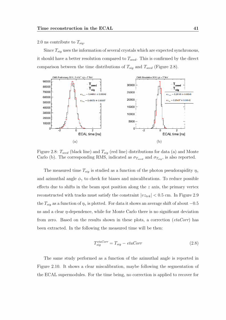
2.0 ns contribute to Tsig.
Since Tsig uses the information of several crystals which are expected synchronous,
it should have a better resolution compared to Tseed. This is confirmed by the direct
comparison between the time distributions of Tsig and Tseed (Figure 2.8).
(a) (b)
Figure 2.8: Tseed (black line) and Tsig (red line) distributions for data (a) and MonteCarlo (b). The corresponding RMS, indicated as σTseed and σTsig , is also reported.
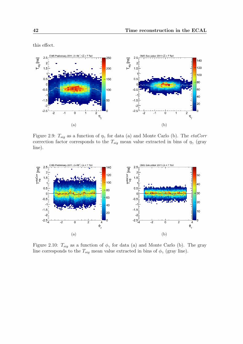
The measured time Tsig is studied as a function of the photon pseudorapidity ηγ
and azimuthal angle φγ to check for biases and miscalibrations. To reduce possible
effects due to shifts in the beam spot position along the z axis, the primary vertex
reconstructed with tracks must satisfy the constraint |vztrk| < 0.5 cm. In Figure 2.9
the Tsig as a function of ηγ is plotted. For data it shows an average shift of about−0.5
ns and a clear η-dependence, while for Monte Carlo there is no significant deviation
from zero. Based on the results shown in these plots, a correction (etaCorr) has
been extracted. In the following the measured time will be then:
T etaCorrsig = Tsig − etaCorr (2.8)
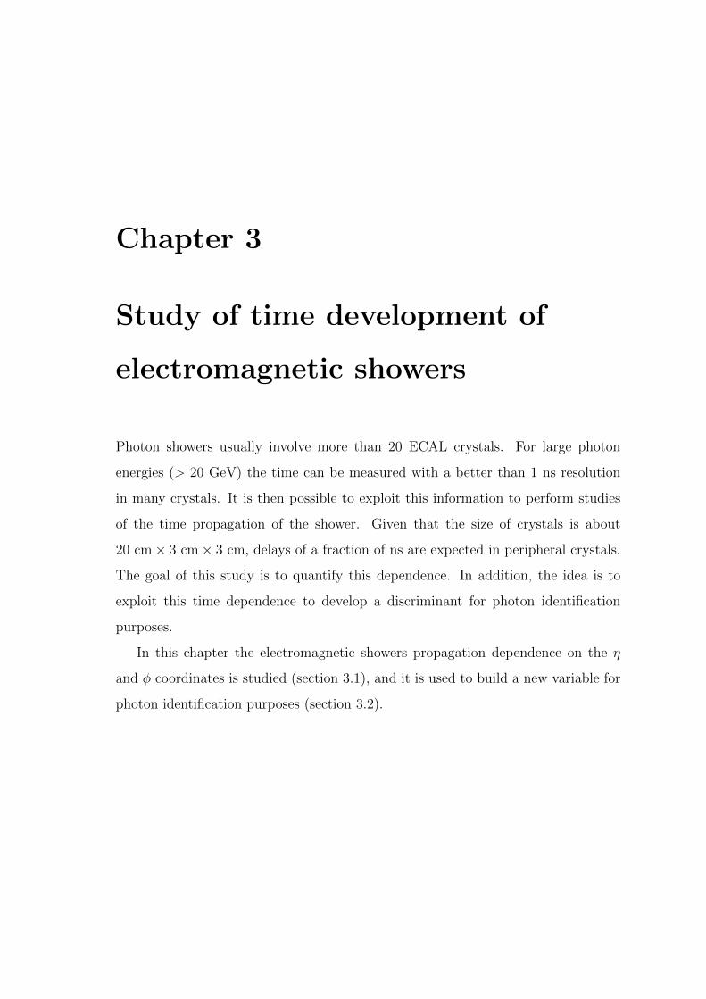
The same study performed as a function of the azimuthal angle is reported in
Figure 2.10. It shows a clear miscalibration, maybe following the segmentation of
the ECAL supermodules. For the time being, no correction is applied to recover for
42 Time reconstruction in the ECAL
this effect.
(a) (b)
Figure 2.9: Tsig as a function of ηγ for data (a) and Monte Carlo (b). The etaCorrcorrection factor corresponds to the Tsig mean value extracted in bins of ηγ (grayline).
(a) (b)
Figure 2.10: Tsig as a function of φγ for data (a) and Monte Carlo (b). The grayline corresponds to the Tsig mean value extracted in bins of φγ (gray line).
Chapter 3
Study of time development of
electromagnetic showers
Photon showers usually involve more than 20 ECAL crystals. For large photon
energies (> 20 GeV) the time can be measured with a better than 1 ns resolution
in many crystals. It is then possible to exploit this information to perform studies
of the time propagation of the shower. Given that the size of crystals is about
20 cm× 3 cm× 3 cm, delays of a fraction of ns are expected in peripheral crystals.
The goal of this study is to quantify this dependence. In addition, the idea is to
exploit this time dependence to develop a discriminant for photon identification
purposes.
In this chapter the electromagnetic showers propagation dependence on the η
and φ coordinates is studied (section 3.1), and it is used to build a new variable for
photon identification purposes (section 3.2).
44 Study of time development of electromagnetic showers
3.1 Electromagnetic showers propagation in the
ECAL
The study is first performed on simulation. This is because we want to start from
a pure sample of photons identified using Monte Carlo truth information. Events
with at least one photon with pT > 30 GeV/c and |η| < 1.4 (barrel) are selected.
Since Monte Carlo truth matching is used, the isolation criteria in order to select
photons are not necessary. We also build a sample of fake photons originated from
misidentified jets. The definitions of the two samples are the following:
• good photon − the reconstructed photon is compared with each gener-
ated photon, computing the variable ∆R(γreco, γgen) =√
∆η2 + ∆φ2 for each
(γreco, γgen) pair. ∆η = ηγreco − ηγgen, ∆φ = φγreco − φγgen, and ηγreco (ηγgen), φγreco
(φγgen) are the pseudorapidity and the φ coordinate of the reconstructed (gen-
erated) photon, respectively. The reconstructed candidate with the minimum
∆R(γreco, γgen) is chosen. If ∆R(γreco, γgen) < 0.1 the photon is selected as a
good photon. A further requirement on ∆R(γreco, jetgen) > 0.3 is applied in
order to minimize the combinatorial background from jets.
• fake photon − the reconstructed photon is matched with a generated jet
(∆R(γreco, jetgen) < 0.1) and does not overlap with a generated photon (∆R(γreco, γgen) >
0.3). In addition, the reconstructed photon must fail the HCAL isolation de-
fined in section 1.3.5.
When a photon hits the ECAL, it creates an electromagnetic shower. The re-
sulting supercluster consists of a cluster of crystals and in each crystal the time is
measured. We expect that the larger the distance of the crystal from the photon
impact point, the larger the time difference compared to the crystal seed. In other
words, the difference ∆Ti = Txtal,i − Tseed increases as the differences ηxtal,i − ηSCand φxtal,i − φSC increase.
Study of time development of electromagnetic showers 45
∆Ti is studied as a function of two variables defined as:
∆ηi =ηxtal,i − ηSC
0.0174, ∆φi =
φxtal,i − φSC0.0174
(3.1)
where 0.0174× 0.0174 correspond to the dimensions of the crystal front face in the
η − φ plane. Then, ∆ηi and ∆φi result to be the distance of the crystal from the
impact point position in terms of number of crystals.
The study is performed in strips of η and φ in order to disentangle the effects
along the η and φ coordinates. Then, the requirement that φxtal,i = φSC is applied
when studying the dependence in ∆ηi and the requirement that ηxtal,i = ηSC is
applied when studying the dependence in ∆φi.
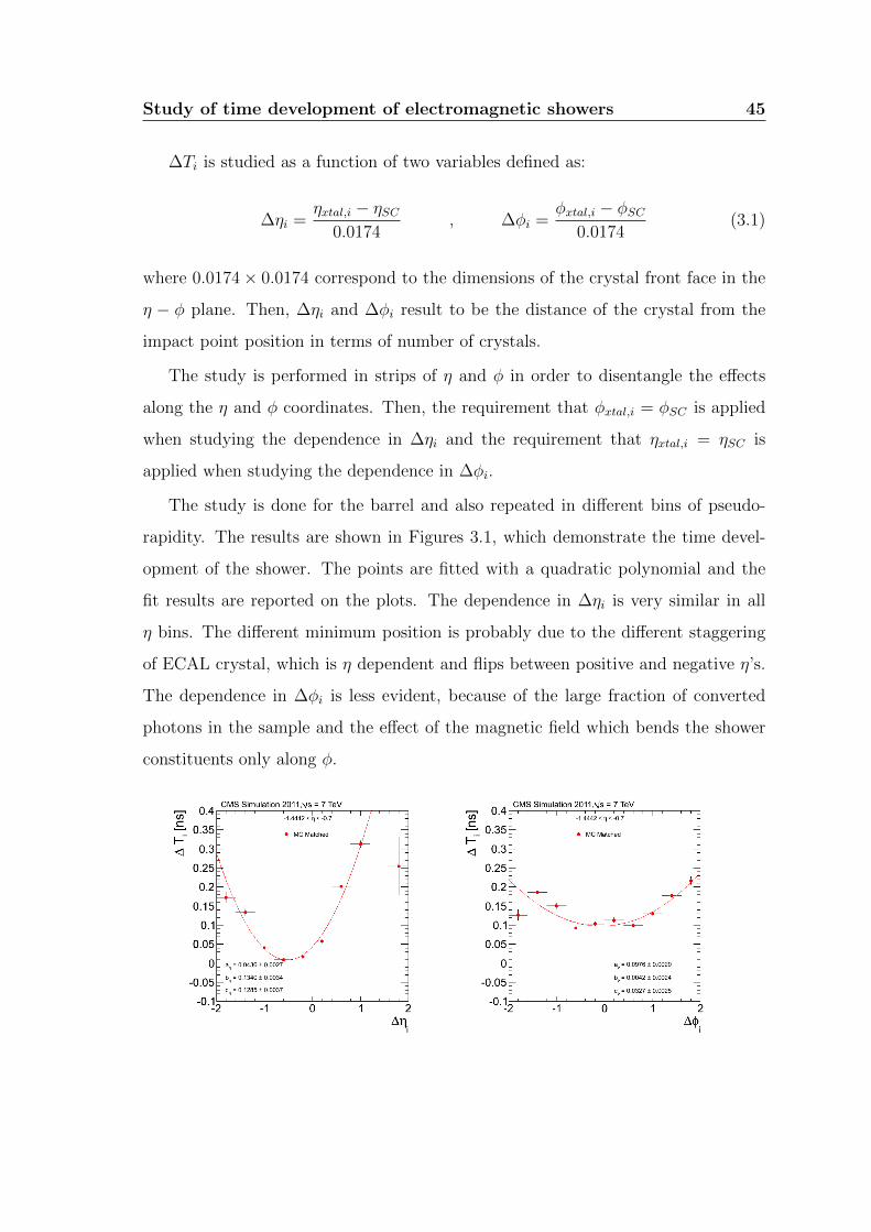
The study is done for the barrel and also repeated in different bins of pseudo-
rapidity. The results are shown in Figures 3.1, which demonstrate the time devel-
opment of the shower. The points are fitted with a quadratic polynomial and the
fit results are reported on the plots. The dependence in ∆ηi is very similar in all
η bins. The different minimum position is probably due to the different staggering
of ECAL crystal, which is η dependent and flips between positive and negative η’s.
The dependence in ∆φi is less evident, because of the large fraction of converted
photons in the sample and the effect of the magnetic field which bends the shower
constituents only along φ.
46 Study of time development of electromagnetic showers
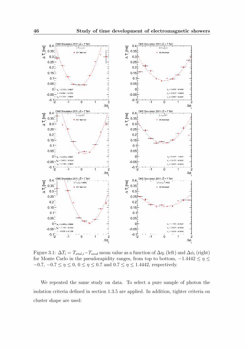
Figure 3.1: ∆Ti = Txtal,i−Tseed mean value as a function of ∆ηi (left) and ∆φi (right)for Monte Carlo in the pseudorapidity ranges, from top to bottom, −1.4442 ≤ η ≤−0.7, −0.7 ≤ η ≤ 0, 0 ≤ η ≤ 0.7 and 0.7 ≤ η ≤ 1.4442, respectively.
We repeated the same study on data. To select a pure sample of photon the
isolation criteria defined in section 1.3.5 are applied. In addition, tighter criteria on
cluster shape are used:
Study of time development of electromagnetic showers 47
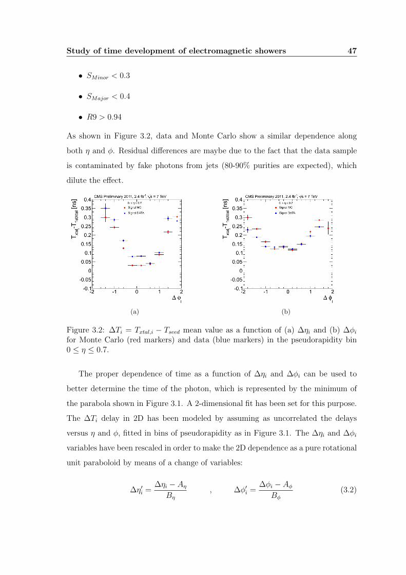
• SMinor < 0.3
• SMajor < 0.4
• R9 > 0.94
As shown in Figure 3.2, data and Monte Carlo show a similar dependence along
both η and φ. Residual differences are maybe due to the fact that the data sample
is contaminated by fake photons from jets (80-90% purities are expected), which
dilute the effect.
(a) (b)
Figure 3.2: ∆Ti = Txtal,i − Tseed mean value as a function of (a) ∆ηi and (b) ∆φifor Monte Carlo (red markers) and data (blue markers) in the pseudorapidity bin0 ≤ η ≤ 0.7.
The proper dependence of time as a function of ∆ηi and ∆φi can be used to
better determine the time of the photon, which is represented by the minimum of
the parabola shown in Figure 3.1. A 2-dimensional fit has been set for this purpose.
The ∆Ti delay in 2D has been modeled by assuming as uncorrelated the delays
versus η and φ, fitted in bins of pseudorapidity as in Figure 3.1. The ∆ηi and ∆φi
variables have been rescaled in order to make the 2D dependence as a pure rotational
unit paraboloid by means of a change of variables:
∆η′i =∆ηi − Aη
Bη
, ∆φ′i =∆φi − Aφ
Bφ
(3.2)
48 Study of time development of electromagnetic showers
The fitted parabolas in Figure 3.1 correspond to:
Txtal,i = aη + bη ∆ηi + cη (∆ηi)2 for ∆φi = 0
Txtal,i = aφ + bφ ∆φi + cφ (∆φi)2 for ∆ηi = 0
(3.3)
where the coefficients aη, bη and cη (aφ, bφ and cφ) are obtained by the fit. After the
translation in equation 3.2, they become:
Txtal,i = (∆η′i)2 for ∆φ′i = 0
Txtal,i = (∆φ′i)2 for ∆η′i = 0
(3.4)
The final 2D parametrization is then:
Txtal,i = (∆η′i)2 + (∆φ′i)
2 + Tfit (3.5)
where Tfit corresponds to the time of the photon.
We use this parametrization to perform a fit based on a χ2 minimization where
the only free parameter is Tfit (Figure 3.3). The χ2time is defined as:
χ2time =
∑i
(Txtal,i − T expxtal,i)2
σ2xtal,i
(3.6)
where i indicates the crystal of the supercluster, Txtal,i is the measured time in that
crystal, T expxtal,i is the expected time as in equation 3.5 and σxtal,i is the expected time
uncertainty as in equation 2.6.
This minimization is run for each photon, thus obtaining the time of the photon
Tfit and the value of the χ2time for the minimum. The probability of the χ2
time is
reported in Figure 3.4(a) and shows a reasonable behavior. The peak at zero is
maybe due to either fake photons or converted photons, where the time dependence
is jeopardized by the presence of a e+e− pair, which distort the ∆Ti along the
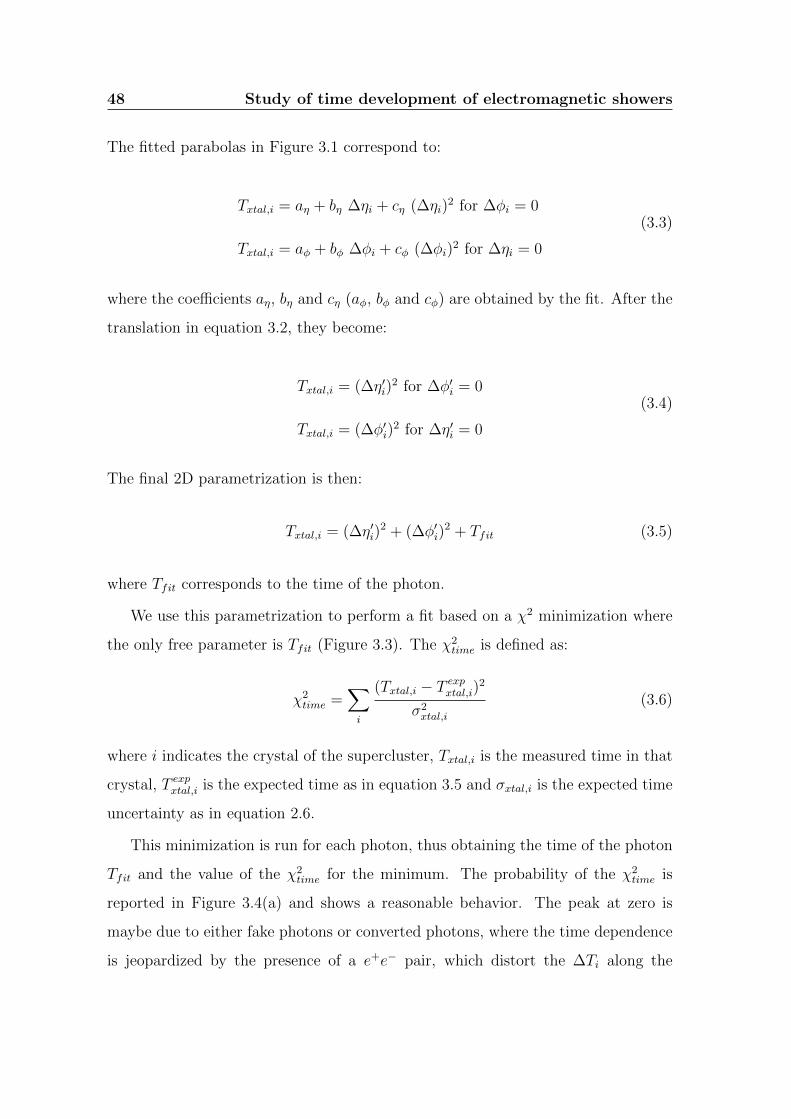
Study of time development of electromagnetic showers 49
Figure 3.3: A map of the crystals in the supercluster in an event. The height of thecolumns is the time measured by the crystals Txtal,i. The red line is the fit functiongiven by equation 3.5.
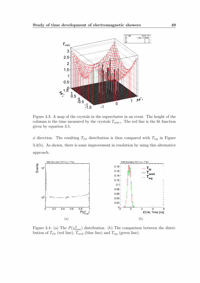
φ direction. The resulting Tfit distribution is then compared with Tsig in Figure
3.4(b). As shown, there is some improvement in resolution by using this alternative
approach.
(a) (b)
Figure 3.4: (a) The P (χ2time) distribution. (b) The comparison between the distri-
bution of Tfit (red line), Tseed (blue line) and Tsig (green line).
50 Study of time development of electromagnetic showers
3.2 A new variable for discrimination between sig-
nal and background
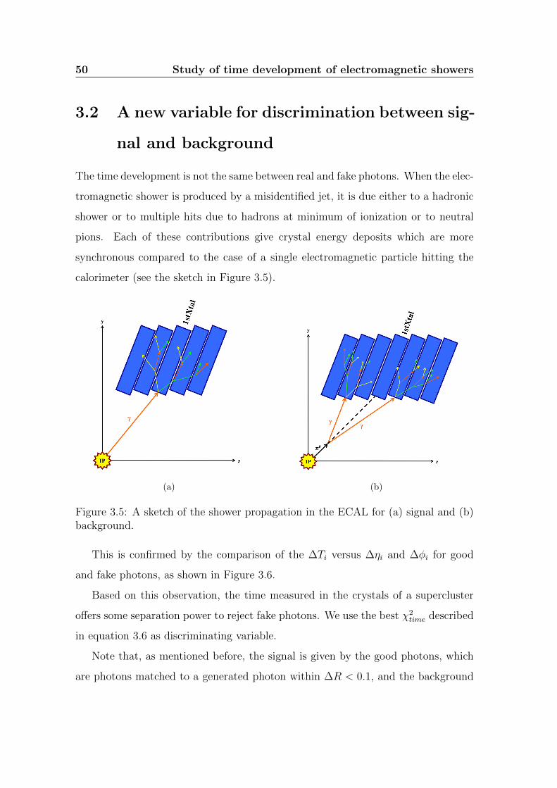
The time development is not the same between real and fake photons. When the elec-
tromagnetic shower is produced by a misidentified jet, it is due either to a hadronic
shower or to multiple hits due to hadrons at minimum of ionization or to neutral
pions. Each of these contributions give crystal energy deposits which are more
synchronous compared to the case of a single electromagnetic particle hitting the
calorimeter (see the sketch in Figure 3.5).
(a) (b)
Figure 3.5: A sketch of the shower propagation in the ECAL for (a) signal and (b)background.
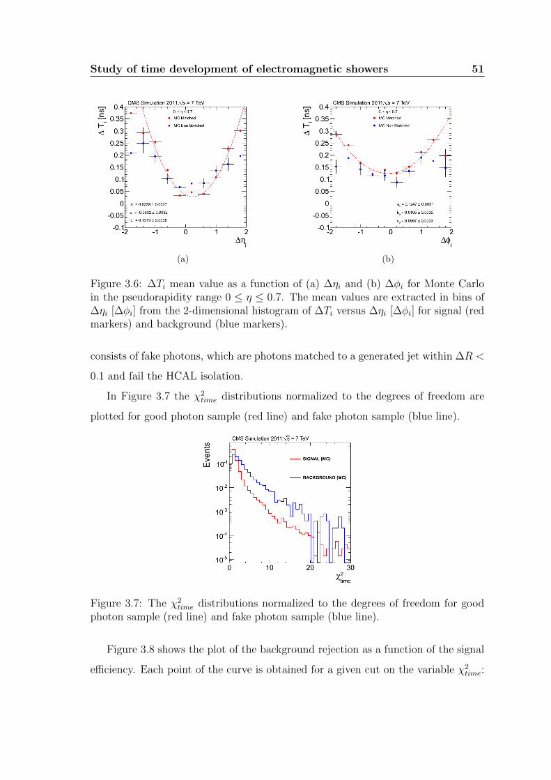
This is confirmed by the comparison of the ∆Ti versus ∆ηi and ∆φi for good
and fake photons, as shown in Figure 3.6.
Based on this observation, the time measured in the crystals of a supercluster
offers some separation power to reject fake photons. We use the best χ2time described
in equation 3.6 as discriminating variable.
Note that, as mentioned before, the signal is given by the good photons, which
are photons matched to a generated photon within ∆R < 0.1, and the background
Study of time development of electromagnetic showers 51
(a) (b)
Figure 3.6: ∆Ti mean value as a function of (a) ∆ηi and (b) ∆φi for Monte Carloin the pseudorapidity range 0 ≤ η ≤ 0.7. The mean values are extracted in bins of∆ηi [∆φi] from the 2-dimensional histogram of ∆Ti versus ∆ηi [∆φi] for signal (redmarkers) and background (blue markers).
consists of fake photons, which are photons matched to a generated jet within ∆R <
0.1 and fail the HCAL isolation.
In Figure 3.7 the χ2time distributions normalized to the degrees of freedom are
plotted for good photon sample (red line) and fake photon sample (blue line).
Figure 3.7: The χ2time distributions normalized to the degrees of freedom for good
photon sample (red line) and fake photon sample (blue line).
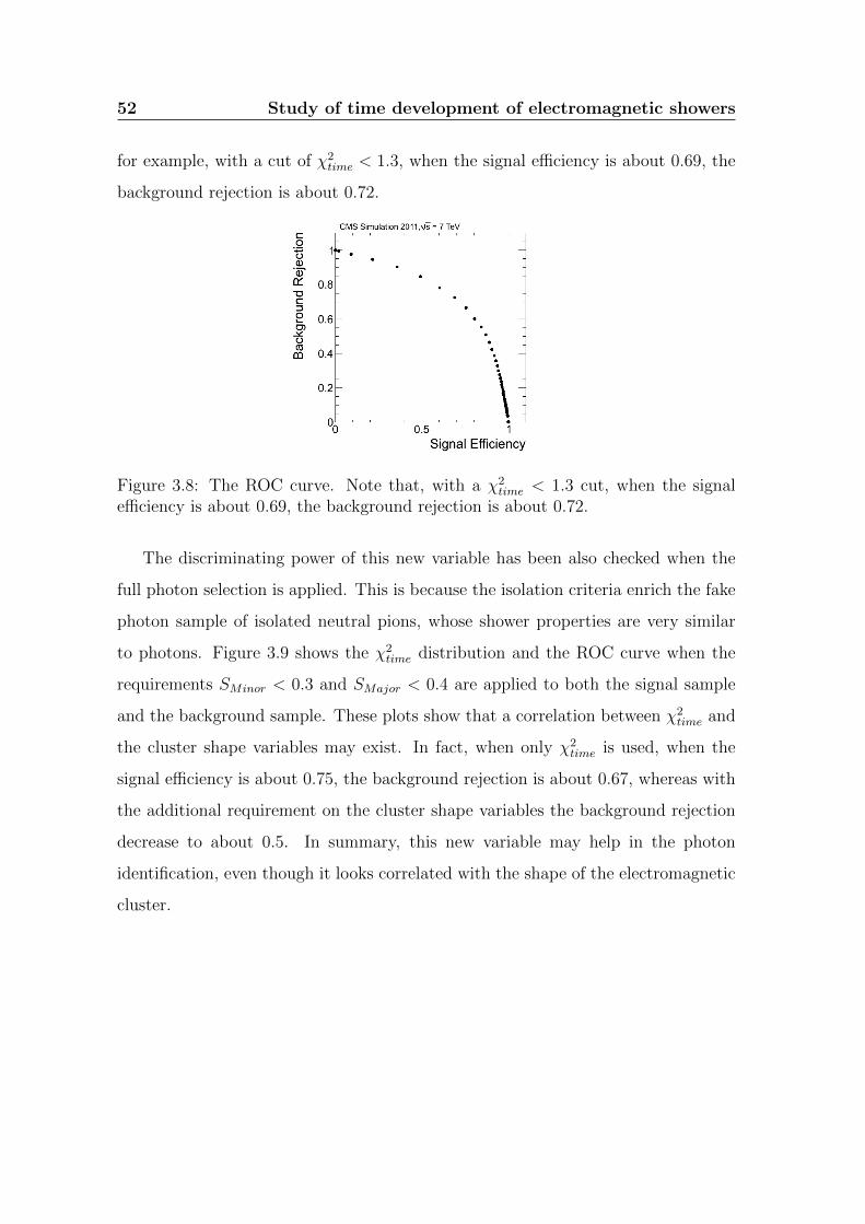
Figure 3.8 shows the plot of the background rejection as a function of the signal
efficiency. Each point of the curve is obtained for a given cut on the variable χ2time:
52 Study of time development of electromagnetic showers
for example, with a cut of χ2time < 1.3, when the signal efficiency is about 0.69, the
background rejection is about 0.72.
Figure 3.8: The ROC curve. Note that, with a χ2time < 1.3 cut, when the signal
efficiency is about 0.69, the background rejection is about 0.72.
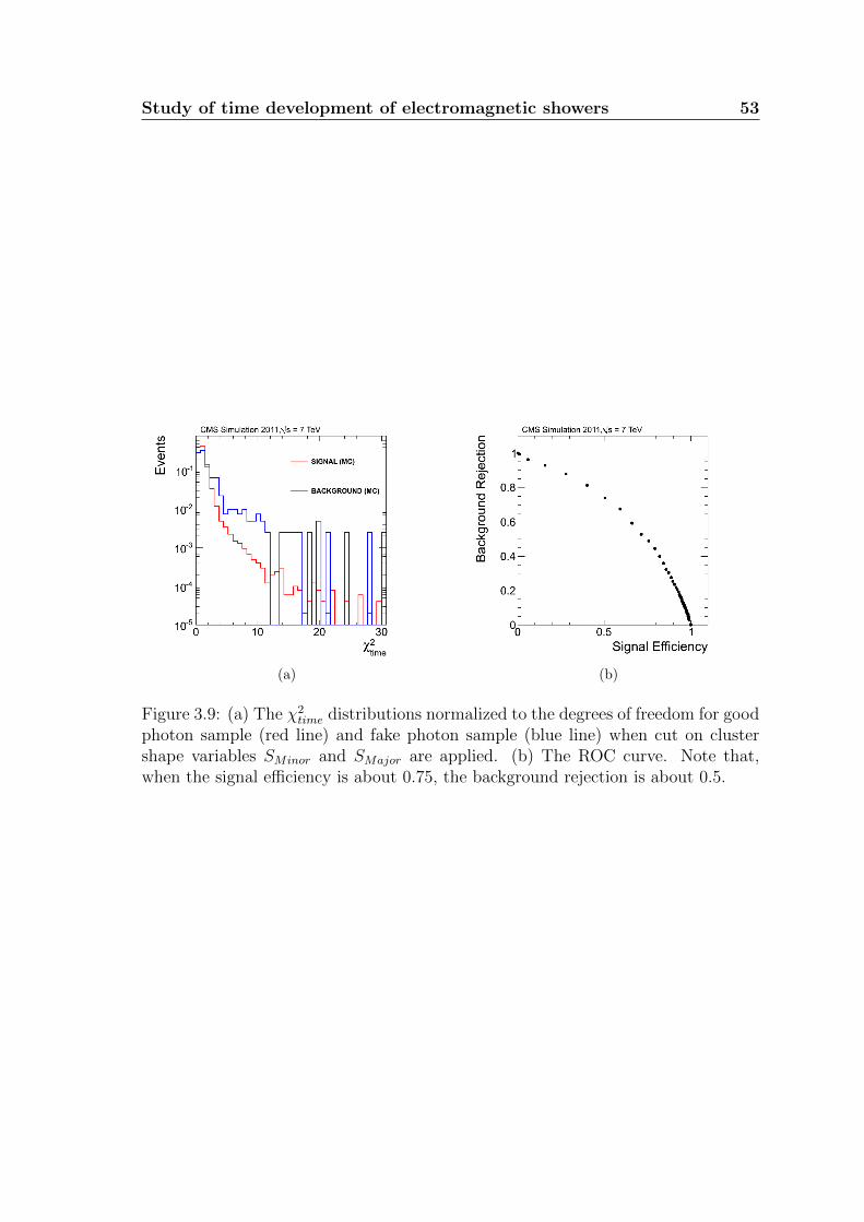
The discriminating power of this new variable has been also checked when the
full photon selection is applied. This is because the isolation criteria enrich the fake
photon sample of isolated neutral pions, whose shower properties are very similar
to photons. Figure 3.9 shows the χ2time distribution and the ROC curve when the
requirements SMinor < 0.3 and SMajor < 0.4 are applied to both the signal sample
and the background sample. These plots show that a correlation between χ2time and
the cluster shape variables may exist. In fact, when only χ2time is used, when the
signal efficiency is about 0.75, the background rejection is about 0.67, whereas with
the additional requirement on the cluster shape variables the background rejection
decrease to about 0.5. In summary, this new variable may help in the photon
identification, even though it looks correlated with the shape of the electromagnetic
cluster.
Study of time development of electromagnetic showers 53
(a) (b)
Figure 3.9: (a) The χ2time distributions normalized to the degrees of freedom for good
photon sample (red line) and fake photon sample (blue line) when cut on clustershape variables SMinor and SMajor are applied. (b) The ROC curve. Note that,when the signal efficiency is about 0.75, the background rejection is about 0.5.

Chapter 4
Vertex reconstruction using ECAL
timing information
The identification of vertices plays an important role in the event reconstruction.
Precise coordinates of the primary event vertices are needed to assign tracks to
collisions and to determine the event kinematics. Furthermore, the determination
of secondary vertices is used to determine the presence of particles decaying in
flight, not only Standard Model particles like taus or B hadrons, but also possible
new states [10].
In this work a novel and alternative method is developed to determine the po-
sition of the vertex. The time of arrival measured with the ECAL is used. This
method is completely decoupled from the tracking. It may offer an important alter-
native handle in events where there is a small track activity, like H → γγ, and to
reject noise from pileup.
In this chapter the vertex reconstruction exploiting the timing information from
the ECAL is described. First, the vertex reconstruction algorithm using tracks is
presented (section 4.1). Then, the novel method is discussed (section 4.2). Finally,
an application of this method to the case of Z → ee events is shown (subsection
4.2.1).
56 Vertex reconstruction using ECAL timing information
4.1 Vertex reconstruction with the tracker
Vertex reconstruction made by the tracker [3] [11] usually involves two steps, vertex
finding and vertex fitting. Vertex finding is the task of identifying vertices within
a given set of tracks, such as the track of a jet in case of flavor tagging or the full
event in case of primary vertex finding. So the vertex-finding algorithms can be
very different depending on the physics case. Vertex fitting on the other hand is
the determination of the vertex position assuming it is formed by a given set of
tracks. The goodness of fit may be used to accept or discard a vertex hypothesis. In
addition, the vertex fit is often used to improve the measurement of track parameters
at the vertex.
Track selection, which aims to select tracks produced promptly in the primary
interaction region, imposes requirements on the maximum allowed transverse im-
pact parameter significance with respect to the beamspot, its number of strip and
pixel hits, and its normalized χ2. To ensure high reconstruction efficiency, even in
minimum bias events, there is no requirement on the minimum allowed track pT .
The selected tracks are then clustered, based on their z coordinates at the point
of closest approach to the beamspot. This clustering allows for the possibility of
multiple primary interactions in the same LHC bunch crossing. The clustering al-
gorithm must balance the efficiency for resolving nearby vertices in cases of high
pileup against the possibility of accidentally splitting a single, genuine interaction
vertex into more than one cluster of tracks.
The primary vertex resolution along the z axis is shown in Figure 4.1 as a func-
tion of the number of tracks: the lower the number of tracks using for vertex re-
construction, the worse the resolution on the primary vertex position. In such cases
additional information are needed in order to be able to reconstruct the vertex. For
example, in H → γγ events, the reconstructed primary vertex which most probably
corresponds to the interaction vertex of the diphoton event can be identified using
the kinematic properties of the tracks associated with the vertex and their corre-
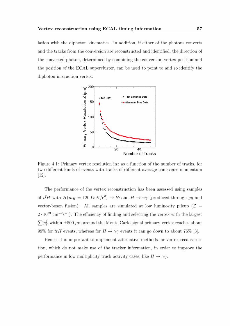
Vertex reconstruction using ECAL timing information 57
lation with the diphoton kinematics. In addition, if either of the photons converts
and the tracks from the conversion are reconstructed and identified, the direction of
the converted photon, determined by combining the conversion vertex position and
the position of the ECAL supercluster, can be used to point to and so identify the
diphoton interaction vertex.
Figure 4.1: Primary vertex resolution inz as a function of the number of tracks, fortwo different kinds of events with tracks of different average transverse momentum[12].
The performance of the vertex reconstruction has been assessed using samples
of ttH with H(mH = 120 GeV/c2) → bb and H → γγ (produced through gg and
vector-boson fusion). All samples are simulated at low luminosity pileup (L =
2 · 1033 cm−2s−1). The efficiency of finding and selecting the vertex with the largest∑p2T within ±500 µm around the Monte Carlo signal primary vertex reaches about
99% for ttH events, whereas for H → γγ events it can go down to about 76% [3].
Hence, it is important to implement alternative methods for vertex reconstruc-
tion, which do not make use of the tracker information, in order to improve the
performance in low multiplicity track activity cases, like H → γγ.
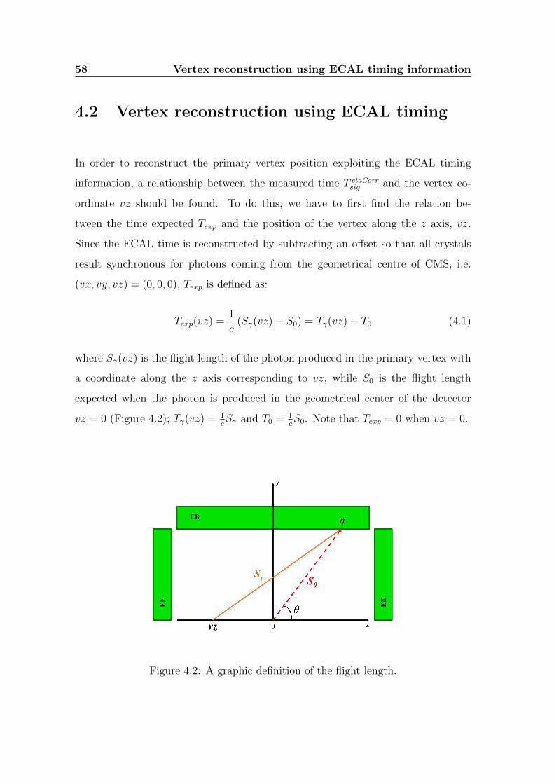
58 Vertex reconstruction using ECAL timing information
4.2 Vertex reconstruction using ECAL timing
In order to reconstruct the primary vertex position exploiting the ECAL timing
information, a relationship between the measured time T etaCorrsig and the vertex co-
ordinate vz should be found. To do this, we have to first find the relation be-
tween the time expected Texp and the position of the vertex along the z axis, vz.
Since the ECAL time is reconstructed by subtracting an offset so that all crystals
result synchronous for photons coming from the geometrical centre of CMS, i.e.
(vx, vy, vz) = (0, 0, 0), Texp is defined as:
Texp(vz) =1
c(Sγ(vz)− S0) = Tγ(vz)− T0 (4.1)
where Sγ(vz) is the flight length of the photon produced in the primary vertex with
a coordinate along the z axis corresponding to vz, while S0 is the flight length
expected when the photon is produced in the geometrical center of the detector
vz = 0 (Figure 4.2); Tγ(vz) = 1cSγ and T0 = 1
cS0. Note that Texp = 0 when vz = 0.
Figure 4.2: A graphic definition of the flight length.
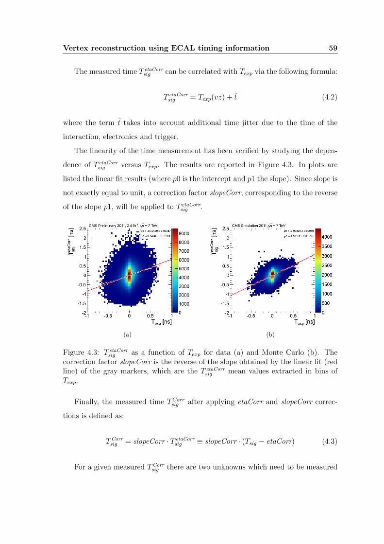
Vertex reconstruction using ECAL timing information 59
The measured time T etaCorrsig can be correlated with Texp via the following formula:
T etaCorrsig = Texp(vz) + t (4.2)
where the term t takes into account additional time jitter due to the time of the
interaction, electronics and trigger.
The linearity of the time measurement has been verified by studying the depen-
dence of T etaCorrsig versus Texp. The results are reported in Figure 4.3. In plots are
listed the linear fit results (where p0 is the intercept and p1 the slope). Since slope is
not exactly equal to unit, a correction factor slopeCorr, corresponding to the reverse
of the slope p1, will be applied to T etaCorrsig .
(a) (b)
Figure 4.3: T etaCorrsig as a function of Texp for data (a) and Monte Carlo (b). The
correction factor slopeCorr is the reverse of the slope obtained by the linear fit (redline) of the gray markers, which are the T etaCorr
sig mean values extracted in bins ofTexp.
Finally, the measured time TCorrsig after applying etaCorr and slopeCorr correc-
tions is defined as:
TCorrsig = slopeCorr · T etaCorr
sig ≡ slopeCorr · (Tsig − etaCorr) (4.3)
For a given measured TCorrsig there are two unknowns which need to be measured
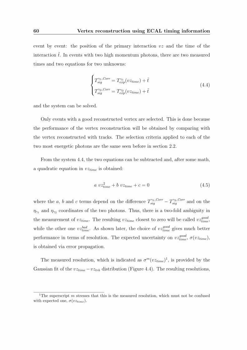
60 Vertex reconstruction using ECAL timing information
event by event: the position of the primary interaction vz and the time of the
interaction t. In events with two high momentum photons, there are two measured
times and two equations for two unknowns:Tγ1,Corrsig = T γ1exp(vztime) + t
T γ2,Corrsig = T γ2exp(vztime) + t
(4.4)
and the system can be solved.
Only events with a good reconstructed vertex are selected. This is done because
the performance of the vertex reconstruction will be obtained by comparing with
the vertex reconstructed with tracks. The selection criteria applied to each of the
two most energetic photons are the same seen before in section 2.2.
From the system 4.4, the two equations can be subtracted and, after some math,
a quadratic equation in vztime is obtained:
a vz2time + b vztime + c = 0 (4.5)
where the a, b and c terms depend on the difference T γ1,Corrsig − T γ2,Corr
sig and on the
ηγ1 and ηγ2 coordinates of the two photons. Thus, there is a two-fold ambiguity in
the measurement of vztime. The resulting vztime closest to zero will be called vzgoodtime,
while the other one vzbadtime. As shown later, the choice of vzgoodtime gives much better
performance in terms of resolution. The expected uncertainty on vzgoodtime, σ(vztime),
is obtained via error propagation.
The measured resolution, which is indicated as σm(vztime)1, is provided by the
Gaussian fit of the vztime−vztrk distribution (Figure 4.4). The resulting resolutions,
1The superscript m stresses that this is the measured resolution, which must not be confusedwith expected one, σ(vztime).
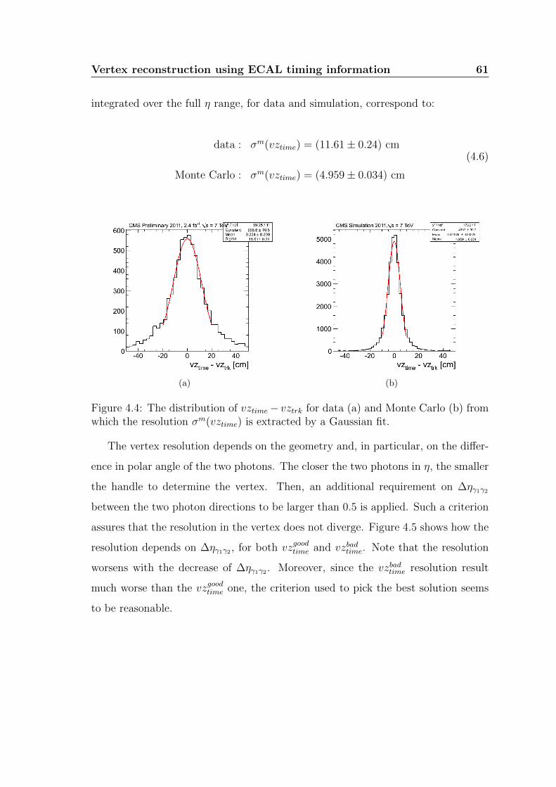
Vertex reconstruction using ECAL timing information 61
integrated over the full η range, for data and simulation, correspond to:
data : σm(vztime) = (11.61± 0.24) cm
Monte Carlo : σm(vztime) = (4.959± 0.034) cm
(4.6)
(a) (b)
Figure 4.4: The distribution of vztime− vztrk for data (a) and Monte Carlo (b) fromwhich the resolution σm(vztime) is extracted by a Gaussian fit.
The vertex resolution depends on the geometry and, in particular, on the differ-
ence in polar angle of the two photons. The closer the two photons in η, the smaller
the handle to determine the vertex. Then, an additional requirement on ∆ηγ1γ2
between the two photon directions to be larger than 0.5 is applied. Such a criterion
assures that the resolution in the vertex does not diverge. Figure 4.5 shows how the
resolution depends on ∆ηγ1γ2 , for both vzgoodtime and vzbadtime. Note that the resolution
worsens with the decrease of ∆ηγ1γ2 . Moreover, since the vzbadtime resolution result
much worse than the vzgoodtime one, the criterion used to pick the best solution seems
to be reasonable.
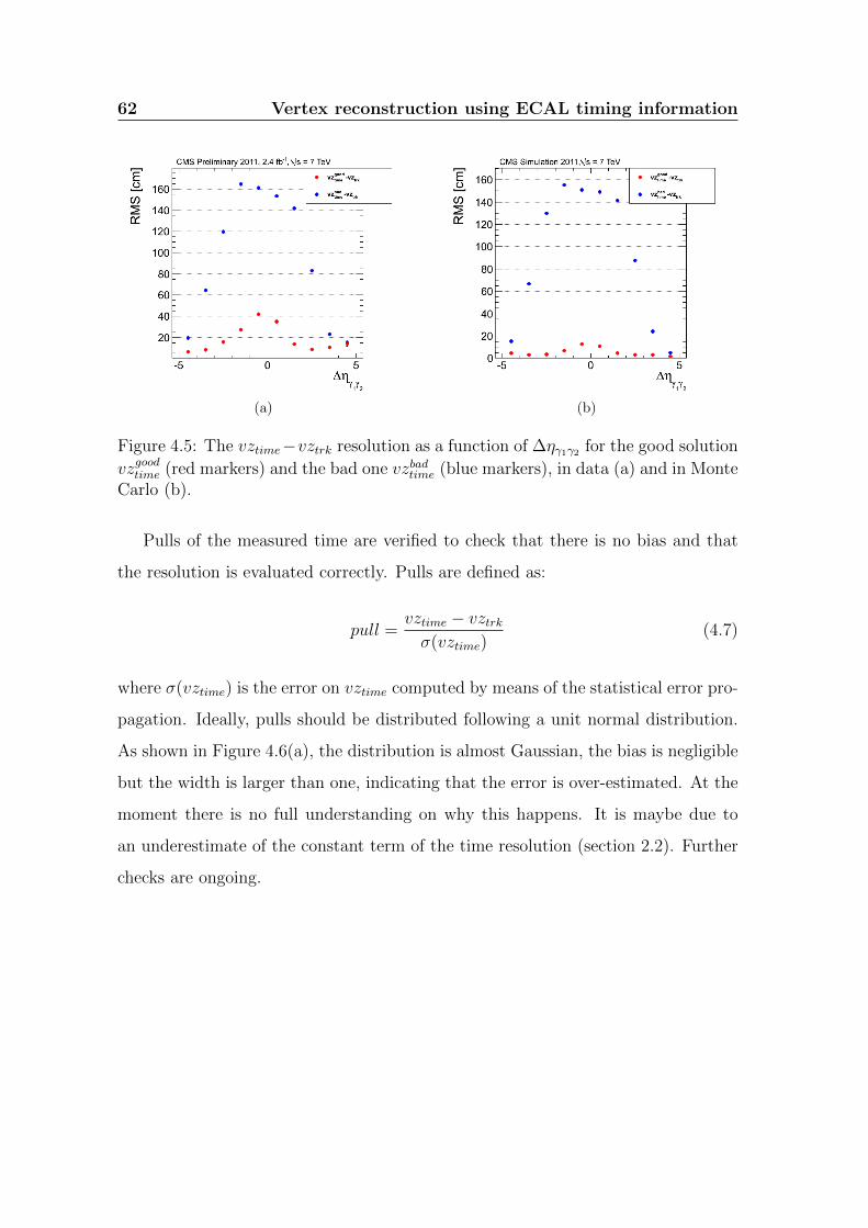
62 Vertex reconstruction using ECAL timing information
(a) (b)
Figure 4.5: The vztime−vztrk resolution as a function of ∆ηγ1γ2 for the good solution
vzgoodtime (red markers) and the bad one vzbadtime (blue markers), in data (a) and in MonteCarlo (b).
Pulls of the measured time are verified to check that there is no bias and that
the resolution is evaluated correctly. Pulls are defined as:
pull =vztime − vztrkσ(vztime)
(4.7)
where σ(vztime) is the error on vztime computed by means of the statistical error pro-
pagation. Ideally, pulls should be distributed following a unit normal distribution.
As shown in Figure 4.6(a), the distribution is almost Gaussian, the bias is negligible
but the width is larger than one, indicating that the error is over-estimated. At the
moment there is no full understanding on why this happens. It is maybe due to
an underestimate of the constant term of the time resolution (section 2.2). Further
checks are ongoing.
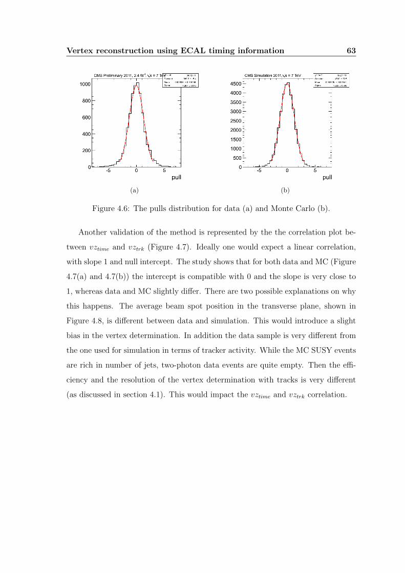
Vertex reconstruction using ECAL timing information 63
(a) (b)
Figure 4.6: The pulls distribution for data (a) and Monte Carlo (b).
Another validation of the method is represented by the the correlation plot be-
tween vztime and vztrk (Figure 4.7). Ideally one would expect a linear correlation,
with slope 1 and null intercept. The study shows that for both data and MC (Figure
4.7(a) and 4.7(b)) the intercept is compatible with 0 and the slope is very close to
1, whereas data and MC slightly differ. There are two possible explanations on why
this happens. The average beam spot position in the transverse plane, shown in
Figure 4.8, is different between data and simulation. This would introduce a slight
bias in the vertex determination. In addition the data sample is very different from
the one used for simulation in terms of tracker activity. While the MC SUSY events
are rich in number of jets, two-photon data events are quite empty. Then the effi-
ciency and the resolution of the vertex determination with tracks is very different
(as discussed in section 4.1). This would impact the vztime and vztrk correlation.
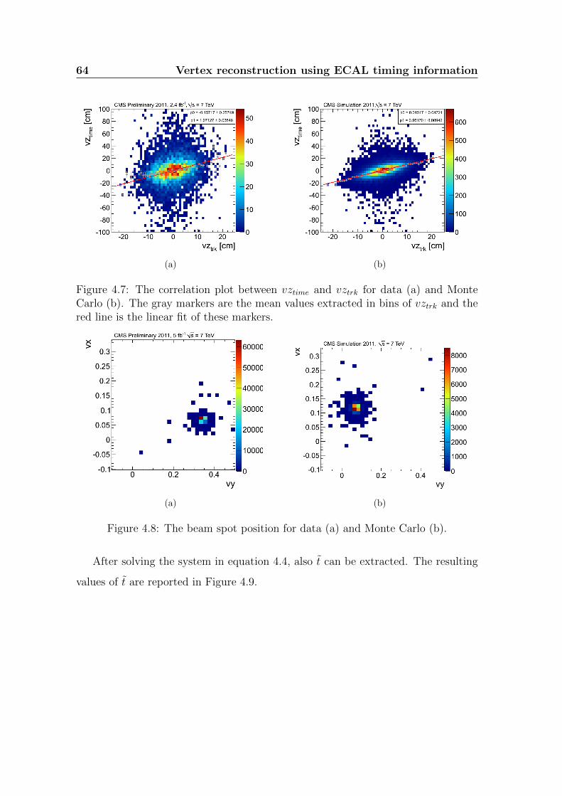
64 Vertex reconstruction using ECAL timing information
(a) (b)
Figure 4.7: The correlation plot between vztime and vztrk for data (a) and MonteCarlo (b). The gray markers are the mean values extracted in bins of vztrk and thered line is the linear fit of these markers.
(a) (b)
Figure 4.8: The beam spot position for data (a) and Monte Carlo (b).
After solving the system in equation 4.4, also t can be extracted. The resulting
values of t are reported in Figure 4.9.
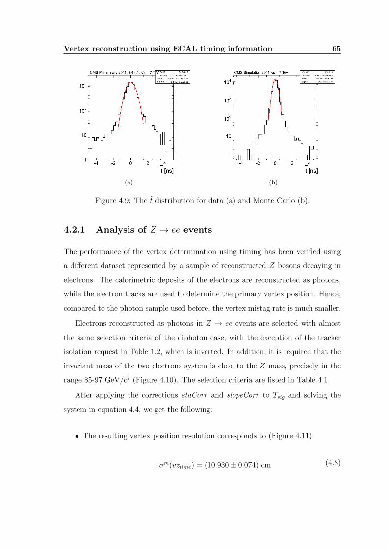
Vertex reconstruction using ECAL timing information 65
(a) (b)
Figure 4.9: The t distribution for data (a) and Monte Carlo (b).
4.2.1 Analysis of Z → ee events
The performance of the vertex determination using timing has been verified using
a different dataset represented by a sample of reconstructed Z bosons decaying in
electrons. The calorimetric deposits of the electrons are reconstructed as photons,
while the electron tracks are used to determine the primary vertex position. Hence,
compared to the photon sample used before, the vertex mistag rate is much smaller.
Electrons reconstructed as photons in Z → ee events are selected with almost
the same selection criteria of the diphoton case, with the exception of the tracker
isolation request in Table 1.2, which is inverted. In addition, it is required that the
invariant mass of the two electrons system is close to the Z mass, precisely in the
range 85-97 GeV/c2 (Figure 4.10). The selection criteria are listed in Table 4.1.
After applying the corrections etaCorr and slopeCorr to Tsig and solving the
system in equation 4.4, we get the following:
• The resulting vertex position resolution corresponds to (Figure 4.11):
σm(vztime) = (10.930± 0.074) cm (4.8)
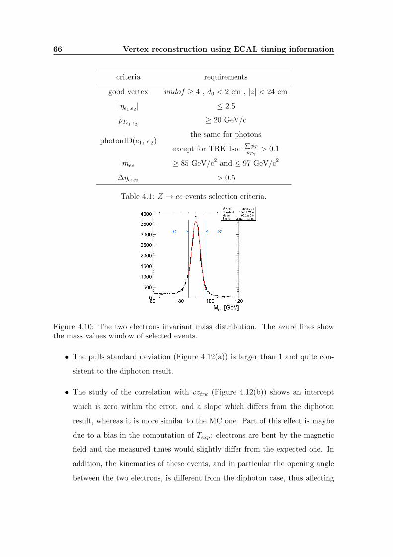
66 Vertex reconstruction using ECAL timing information
criteria requirements
good vertex vndof ≥ 4 , d0 < 2 cm , |z| < 24 cm
|ηe1,e2| ≤ 2.5
pTe1,e2 ≥ 20 GeV/c
photonID(e1, e2)the same for photons
except for TRK Iso:∑pT
pTγ> 0.1
mee ≥ 85 GeV/c2 and ≤ 97 GeV/c2
∆ηe1e2 > 0.5
Table 4.1: Z → ee events selection criteria.
Figure 4.10: The two electrons invariant mass distribution. The azure lines showthe mass values window of selected events.
• The pulls standard deviation (Figure 4.12(a)) is larger than 1 and quite con-
sistent to the diphoton result.
• The study of the correlation with vztrk (Figure 4.12(b)) shows an intercept
which is zero within the error, and a slope which differs from the diphoton
result, whereas it is more similar to the MC one. Part of this effect is maybe
due to a bias in the computation of Texp: electrons are bent by the magnetic
field and the measured times would slightly differ from the expected one. In
addition, the kinematics of these events, and in particular the opening angle
between the two electrons, is different from the diphoton case, thus affecting
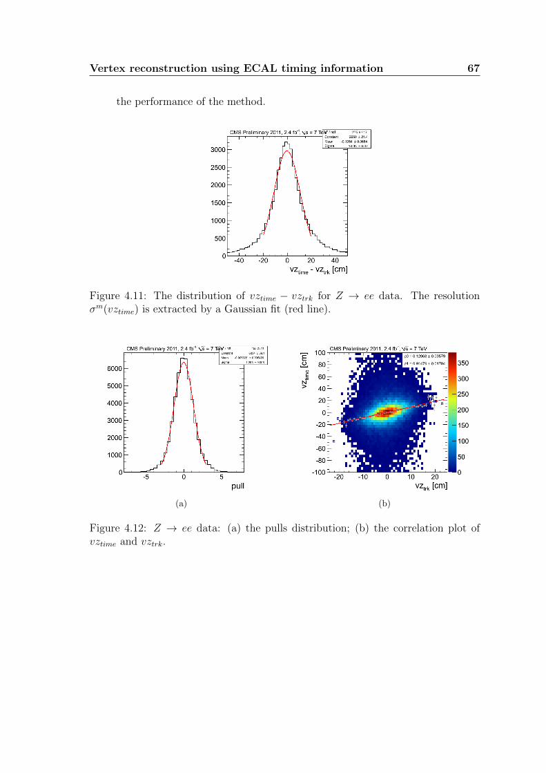
Vertex reconstruction using ECAL timing information 67
the performance of the method.
Figure 4.11: The distribution of vztime − vztrk for Z → ee data. The resolutionσm(vztime) is extracted by a Gaussian fit (red line).
(a) (b)
Figure 4.12: Z → ee data: (a) the pulls distribution; (b) the correlation plot ofvztime and vztrk.

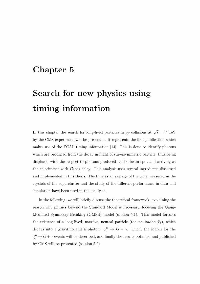
Chapter 5
Search for new physics using
timing information
In this chapter the search for long-lived particles in pp collisions at√s = 7 TeV
by the CMS experiment will be presented. It represents the first publication which
makes use of the ECAL timing information [14]. This is done to identify photons
which are produced from the decay in flight of supersymmetric particle, thus being
displaced with the respect to photons produced at the beam spot and arriving at
the calorimeter with O(ns) delay. This analysis uses several ingredients discussed
and implemented in this thesis. The time as an average of the time measured in the
crystals of the supercluster and the study of the different performance in data and
simulation have been used in this analysis.
In the following, we will briefly discuss the theoretical framework, explaining the
reason why physics beyond the Standard Model is necessary, focusing the Gauge
Mediated Symmetry Breaking (GMSB) model (section 5.1). This model foresees
the existence of a long-lived, massive, neutral particle (the neutralino χ01), which
decays into a gravitino and a photon: χ01 → G + γ. Then, the search for the
χ01 → G+ γ events will be described, and finally the results obtained and published
by CMS will be presented (section 5.2).
70 Search for new physics using timing information
5.1 Theoretical framework
The Standard Model (SM) of elementary particles and their fundamental interac-
tions provides a very elegant theoretical framework, and has been verified with high
accuracy by several experiments, showing an excellent agreement between theoret-
ical expectations and experimental results. Today, the SM is a well established
theory applicable over a wide range of conditions.
Despite the striking experimental success of the SM, this theory still has some
unsolved problems, which range from the origin of particle masses to the nature of
the Dark Matter in the Universe, and represents a strong conceptual indication for
new physics in the TeV energy domain.
Recent theoretical and experimental advances have brought a new focus on the-
oretical proposals for physics beyond the SM with massive and long-lived particles,
which are common in several Supersymmetry (SUSY) models and also in more ex-
otic scenarios. From an experimental point of view, models with long-lived particles
decaying into an energetic photon are very accredited for early discoveries of new
physics from the experiments at the LHC. The analysis discussed here regards SUSY
theories with Gauge Mediated Supersymmetry Breaking (GMSB), since they have
a relatively high production cross section and have a very distinctive experimental
signature. According to the choice of the parameters, GMSB model foresees the
existence of a long-lived, massive, neutral particle (the neutralino χ01), which decays
into a high energy photon and a gravitino G. Since the neutralino can have non-zero
lifetime, the photons from the χ01 → G+ γ decay reaches the ECAL later than pho-
tons produced at the bunch crossing, the so-called prompt photons. The gravitino
is stable and weakly interacting, usually escaping from detection, and so it can be
considered as a massive neutrino.
Search for new physics using timing information 71
5.1.1 The Standard Model and its limits
The SM of particle physics [15] is the successful theory which describes three of
the four fundamental forces, i.e. strong, weak and electromagnetic interactions (the
gravitational one is not included in this model), and the basic constituents of matter.
It has been carefully verified by experiments from the 60’s until now, in particular
with measurements made by the LEP experiment of the CERN in Geneva. It is a
gauge theory, namely a theory which is invariant under a set of space-time dependent
transformations (called local transformations). According to the gauge principle, the
forces are mediated by the exchange of the gauge fields, corresponding to a specific
symmetry group. The mediators associated to the symmetry group are 12 spin-1
gauge bosons: 8 bosons (gluons) for SU(3)C , 3 bosons (Wi) for SU(2)L, and 1 boson
(B) for U(1)Y .
The W± bosons are obtained as a linear combination of W1 and W2, while the Z
boson and the photon γ can be seen as a linear combination of W3 and B. The gluons
are massless, electrically neutral and carry color quantum number. The consequence
of gluons being colorful is that they can interact with each other. The weak bosons
W± and Z are massive particles and also self-interacting. The photon γ is massless,
chargeless and non-selfinteracting. Matter fields are represented by spin-12
leptons
and quarks, organized in three families with identical properties, except for mass.
In Figure 5.1 is shown the three matter generations and the gauge bosons.
In the SM mass terms are introduced by means of the so-called Higgs mechanism
[16] [17], which predicts the existence of a new particle, the Higgs boson: gauge
bosons (except photons), leptons and quarks acquire mass interacting with the Higgs
field.
The Higgs particle is an elementary particle, a massive boson which has no spin,
electric charge or color charge. It is also very unstable, decaying into other particles
almost immediately. Its existence is predicted for theoretical reasons, and it may
have been detected by experiments at the Large Hadron Collider in Geneva. On 4
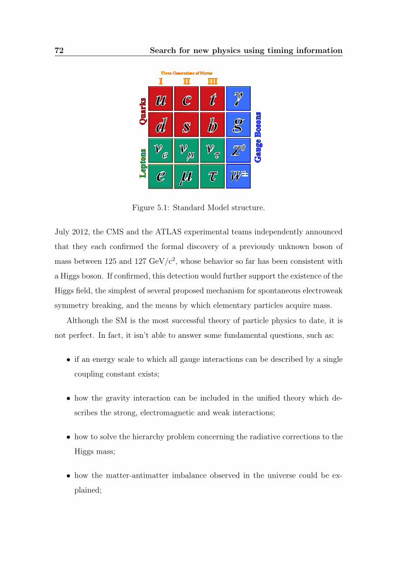
72 Search for new physics using timing information
Figure 5.1: Standard Model structure.
July 2012, the CMS and the ATLAS experimental teams independently announced
that they each confirmed the formal discovery of a previously unknown boson of
mass between 125 and 127 GeV/c2, whose behavior so far has been consistent with
a Higgs boson. If confirmed, this detection would further support the existence of the
Higgs field, the simplest of several proposed mechanism for spontaneous electroweak
symmetry breaking, and the means by which elementary particles acquire mass.
Although the SM is the most successful theory of particle physics to date, it is
not perfect. In fact, it isn’t able to answer some fundamental questions, such as:
• if an energy scale to which all gauge interactions can be described by a single
coupling constant exists;
• how the gravity interaction can be included in the unified theory which de-
scribes the strong, electromagnetic and weak interactions;
• how to solve the hierarchy problem concerning the radiative corrections to the
Higgs mass;
• how the matter-antimatter imbalance observed in the universe could be ex-
plained;
Search for new physics using timing information 73
• which could be a good candidate to the dark matter, which is non-relativistic,
non-barionic, non-luminous and weakly interacting.
Then, answers to these lacks should be found. Different alternative models have
been proposed to date, such as the String theory and the Extradimensions. Among
these, the Supersymmetry is considered the most plausible theory to search for new
physics. From an experimental point of view, the SUSY models are favored because
they have non negligible cross sections and relatively small SM background.
5.1.2 Models with long-lived particles
Recent theoretical and experimental advances have brought a new focus on mod-
els beyond the SM with massive, long-lived particles. Such particles are common
in several SUSY scenarios [18]. According to the characteristics of the long-lived
particle, three main categories has been identified.
Charged particles In many SUSY models, charged particles with large lifetime,
due to small decay phase space, are expected to exist. They mimic the case of very
high momentum muons, crossing the detector with velocity significantly lower than
the speed of light. This unique signature makes the search for it a model-independent
search, based on measurement of both the time of flight and the energy loss by
ionization. In this context, only those models with a gravitino G (the supersimmetric
partner of graviton) in the final state are considered.
Colored particles A long-lived, colored gluino g is a generic prediction of several
models of physics beyond the SM. In this scenarios, g decays into scalar particles
are forbidden and gluinos acquire a macroscopic lifetime. During this time, they
can hadronize into the so-called R-hadrons, bounds states of the gluino and quarks
or gluons. R-hadrons live long inside the detector and, in case they are electrically
charged, can lose all their momentum via ionization and come at rest.
74 Search for new physics using timing information
These particles, commonly referred as stopped gluinos, can decay after a long
time via:
g → g + χ01 (5.1)
where χ01 is a massive and weak interacting exotic particle called neutralino, and g is
a gluon which hadronizes into a jet. Stopped gluinos provide a striking experimen-
tal signature, established by a large amount of delayed hadronic activity without
anything else.
Neutral particles The primary motivation to look for massive neutral particles
with large lifetime is provided by the GMSB model, although they can also be
present in other models, such as hidden valleys scenarios [19]. For what concern
the analysis here presented, the attention will be focused on GMSB model with
long-lived neutralino decaying into a gravitino and a high-energy photon:
χ01 → G+ γ (5.2)
The combination of displaced decay photons and significant energy imbalance in the
transverse plane (due to gravitino which escapes from detection) generally leads to
extremely clean, nearly background-free analysis.
The GMSB model is one of the mechanism for soft supersymmetry breaking that
produces the desired properties in the Minimal Supersymmetric Standard Model
(MSSM) [20]. This is the natural extension of the SM to the supersymmetries
which involves the smallest possible number of new particles: each SM particle has
a supersymmetric partner, and they differ by a half unit of spin (Figure 5.2).
If the SUSY were an exact symmetry of nature, particles and superparticles
would have same masses. This would imply that also the superparticles have al-
ready been discovered. Not being so, then the SUSY is clearly a symmetry broken
through some mechanism: the superpartners of the SM particles result much heavier
and hence not yet discovered. Due to the symmetry breaking, the MSSM states can
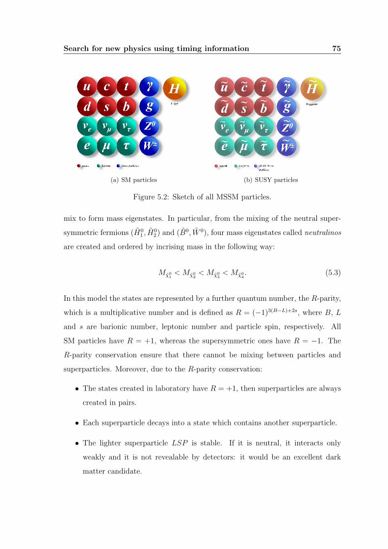
Search for new physics using timing information 75
(a) SM particles (b) SUSY particles
Figure 5.2: Sketch of all MSSM particles.
mix to form mass eigenstates. In particular, from the mixing of the neutral super-
symmetric fermions (H01 , H
02 ) and (B0, W 0), four mass eigenstates called neutralinos
are created and ordered by incrising mass in the following way:
Mχ01< Mχ0
2< Mχ0
3< Mχ0
4. (5.3)
In this model the states are represented by a further quantum number, the R-parity,
which is a multiplicative number and is defined as R = (−1)3(B−L)+2s, where B, L
and s are barionic number, leptonic number and particle spin, respectively. All
SM particles have R = +1, whereas the supersymmetric ones have R = −1. The
R-parity conservation ensure that there cannot be mixing between particles and
superparticles. Moreover, due to the R-parity conservation:
• The states created in laboratory have R = +1, then superparticles are always
created in pairs.
• Each superparticle decays into a state which contains another superparticle.
• The lighter superparticle LSP is stable. If it is neutral, it interacts only
weakly and it is not revealable by detectors: it would be an excellent dark
matter candidate.
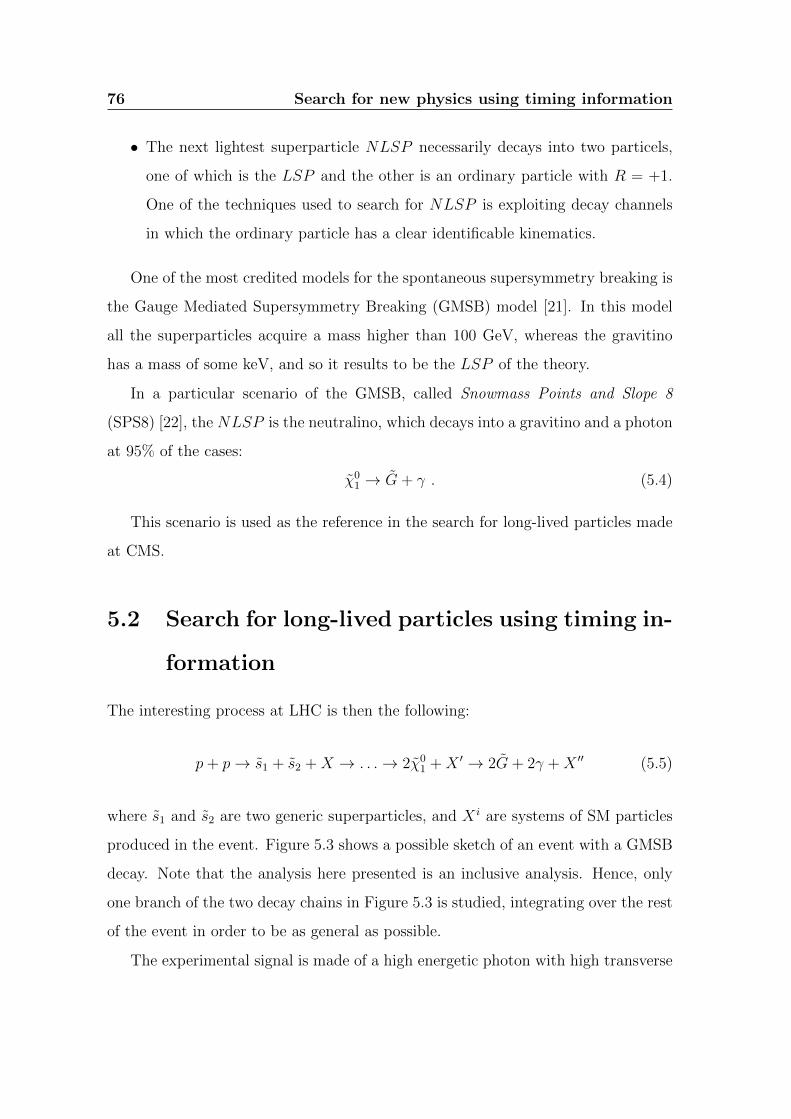
76 Search for new physics using timing information
• The next lightest superparticle NLSP necessarily decays into two particels,
one of which is the LSP and the other is an ordinary particle with R = +1.
One of the techniques used to search for NLSP is exploiting decay channels
in which the ordinary particle has a clear identificable kinematics.
One of the most credited models for the spontaneous supersymmetry breaking is
the Gauge Mediated Supersymmetry Breaking (GMSB) model [21]. In this model
all the superparticles acquire a mass higher than 100 GeV, whereas the gravitino
has a mass of some keV, and so it results to be the LSP of the theory.
In a particular scenario of the GMSB, called Snowmass Points and Slope 8
(SPS8) [22], the NLSP is the neutralino, which decays into a gravitino and a photon
at 95% of the cases:
χ01 → G+ γ . (5.4)
This scenario is used as the reference in the search for long-lived particles made
at CMS.
5.2 Search for long-lived particles using timing in-
formation
The interesting process at LHC is then the following:
p+ p→ s1 + s2 +X → . . .→ 2χ01 +X ′ → 2G+ 2γ +X ′′ (5.5)
where s1 and s2 are two generic superparticles, and X i are systems of SM particles
produced in the event. Figure 5.3 shows a possible sketch of an event with a GMSB
decay. Note that the analysis here presented is an inclusive analysis. Hence, only
one branch of the two decay chains in Figure 5.3 is studied, integrating over the rest
of the event in order to be as general as possible.
The experimental signal is made of a high energetic photon with high transverse
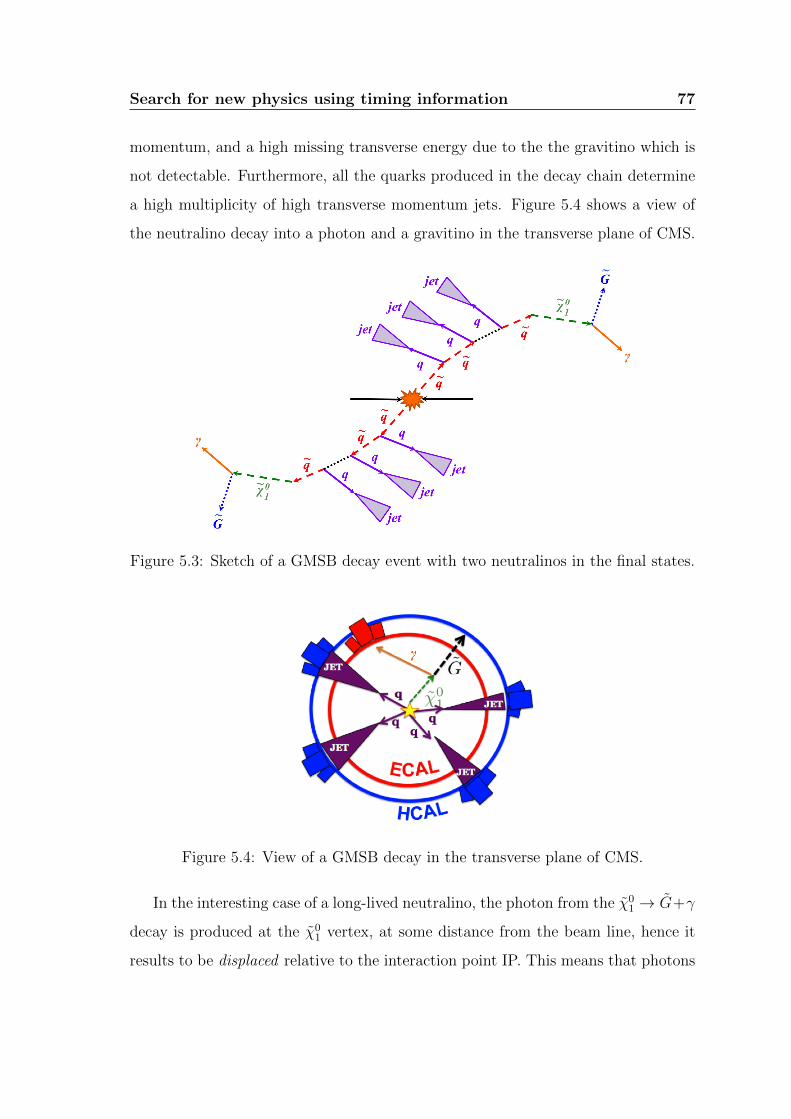
Search for new physics using timing information 77
momentum, and a high missing transverse energy due to the the gravitino which is
not detectable. Furthermore, all the quarks produced in the decay chain determine
a high multiplicity of high transverse momentum jets. Figure 5.4 shows a view of
the neutralino decay into a photon and a gravitino in the transverse plane of CMS.
Figure 5.3: Sketch of a GMSB decay event with two neutralinos in the final states.
Figure 5.4: View of a GMSB decay in the transverse plane of CMS.
In the interesting case of a long-lived neutralino, the photon from the χ01 → G+γ
decay is produced at the χ01 vertex, at some distance from the beam line, hence it
results to be displaced relative to the interaction point IP. This means that photons
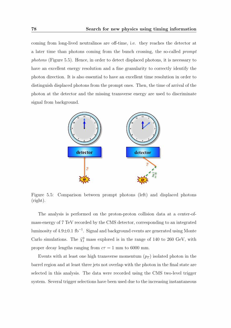
78 Search for new physics using timing information
coming from long-lived neutralinos are off-time, i.e. they reaches the detector at
a later time than photons coming from the bunch crossing, the so-called prompt
photons (Figure 5.5). Hence, in order to detect displaced photons, it is necessary to
have an excellent energy resolution and a fine granularity to correctly identify the
photon direction. It is also essential to have an excellent time resolution in order to
distinguish displaced photons from the prompt ones. Then, the time of arrival of the
photon at the detector and the missing transverse energy are used to discriminate
signal from background.
Figure 5.5: Comparison between prompt photons (left) and displaced photons(right).
The analysis is performed on the proton-proton collision data at a center-of-
mass-energy of 7 TeV recorded by the CMS detector, corresponding to an integrated
luminosity of 4.9±0.1 fb−1. Signal and background events are generated using Monte
Carlo simulations. The χ01 mass explored is in the range of 140 to 260 GeV, with
proper decay lengths ranging from cτ = 1 mm to 6000 mm.
Events with at least one high transverse momentum (pT ) isolated photon in the
barrel region and at least three jets not overlap with the photon in the final state are
selected in this analysis. The data were recorded using the CMS two-level trigger
system. Several trigger selections have been used due to the increasing instantaneous
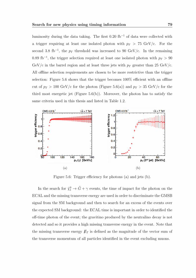
Search for new physics using timing information 79
luminosity during the data taking. The first 0.20 fb−1 of data were collected with
a trigger requiring at least one isolated photon with pT > 75 GeV/c. For the
second 3.8 fb−1, the pT threshold was increased to 90 GeV/c. In the remaining
0.89 fb−1, the trigger selection required at least one isolated photon with pT > 90
GeV/c in the barrel region and at least three jets with pT greater than 25 GeV/c.
All offline selection requirements are chosen to be more restrictive than the trigger
selection: Figure 5.6 shows that the trigger becomes 100% efficient with an offline
cut of pT > 100 GeV/c for the photon (Figure 5.6(a)) and pT > 35 GeV/c for the
third most energetic jet (Figure 5.6(b)). Moreover, the photon has to satisfy the
same criteria used in this thesis and listed in Table 1.2.
(a) (b)
Figure 5.6: Trigger efficiency for photons (a) and jets (b).
In the search for χ01 → G + γ events, the time of impact for the photon on the
ECAL and the missing transverse energy are used in order to discriminate the GMSB
signal from the SM background and then to search for an excess of the events over
the expected SM background: the ECAL time is important in order to identified the
off-time photon of the event; the gravitino produced by the neutralino decay is not
detected and so it provides a high missing transverse energy in the event. Note that
the missing transverse energy 6ET is defined as the magnitude of the vector sum of
the transverse momentum of all particles identified in the event excluding muons.
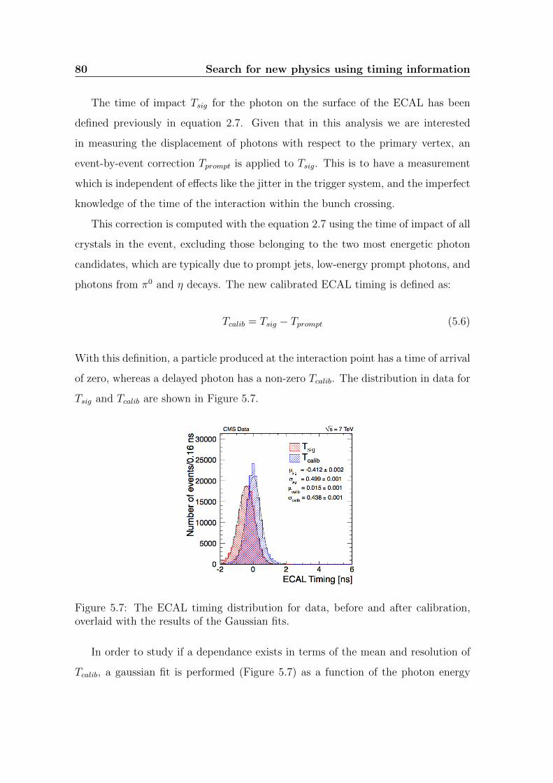
80 Search for new physics using timing information
The time of impact Tsig for the photon on the surface of the ECAL has been
defined previously in equation 2.7. Given that in this analysis we are interested
in measuring the displacement of photons with respect to the primary vertex, an
event-by-event correction Tprompt is applied to Tsig. This is to have a measurement
which is independent of effects like the jitter in the trigger system, and the imperfect
knowledge of the time of the interaction within the bunch crossing.
This correction is computed with the equation 2.7 using the time of impact of all
crystals in the event, excluding those belonging to the two most energetic photon
candidates, which are typically due to prompt jets, low-energy prompt photons, and
photons from π0 and η decays. The new calibrated ECAL timing is defined as:
Tcalib = Tsig − Tprompt (5.6)
With this definition, a particle produced at the interaction point has a time of arrival
of zero, whereas a delayed photon has a non-zero Tcalib. The distribution in data for
Tsig and Tcalib are shown in Figure 5.7.
Figure 5.7: The ECAL timing distribution for data, before and after calibration,overlaid with the results of the Gaussian fits.
In order to study if a dependance exists in terms of the mean and resolution of
Tcalib, a gaussian fit is performed (Figure 5.7) as a function of the photon energy
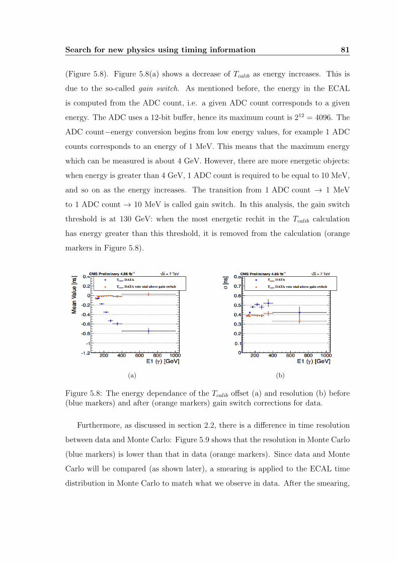
Search for new physics using timing information 81
(Figure 5.8). Figure 5.8(a) shows a decrease of Tcalib as energy increases. This is
due to the so-called gain switch. As mentioned before, the energy in the ECAL
is computed from the ADC count, i.e. a given ADC count corresponds to a given
energy. The ADC uses a 12-bit buffer, hence its maximum count is 212 = 4096. The
ADC count−energy conversion begins from low energy values, for example 1 ADC
counts corresponds to an energy of 1 MeV. This means that the maximum energy
which can be measured is about 4 GeV. However, there are more energetic objects:
when energy is greater than 4 GeV, 1 ADC count is required to be equal to 10 MeV,
and so on as the energy increases. The transition from 1 ADC count → 1 MeV
to 1 ADC count → 10 MeV is called gain switch. In this analysis, the gain switch
threshold is at 130 GeV: when the most energetic rechit in the Tcalib calculation
has energy greater than this threshold, it is removed from the calculation (orange
markers in Figure 5.8).
(a) (b)
Figure 5.8: The energy dependance of the Tcalib offset (a) and resolution (b) before(blue markers) and after (orange markers) gain switch corrections for data.
Furthermore, as discussed in section 2.2, there is a difference in time resolution
between data and Monte Carlo: Figure 5.9 shows that the resolution in Monte Carlo
(blue markers) is lower than that in data (orange markers). Since data and Monte
Carlo will be compared (as shown later), a smearing is applied to the ECAL time
distribution in Monte Carlo to match what we observe in data. After the smearing,
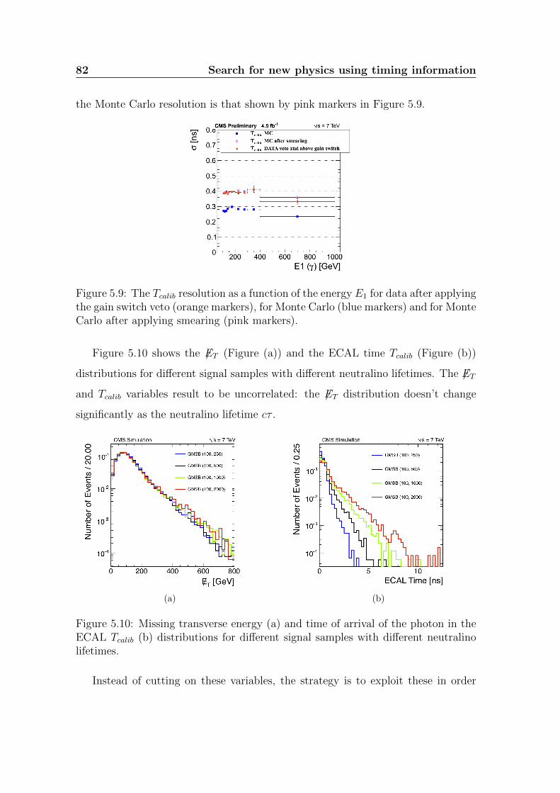
82 Search for new physics using timing information
the Monte Carlo resolution is that shown by pink markers in Figure 5.9.
Figure 5.9: The Tcalib resolution as a function of the energy E1 for data after applyingthe gain switch veto (orange markers), for Monte Carlo (blue markers) and for MonteCarlo after applying smearing (pink markers).
Figure 5.10 shows the 6ET (Figure (a)) and the ECAL time Tcalib (Figure (b))
distributions for different signal samples with different neutralino lifetimes. The 6ETand Tcalib variables result to be uncorrelated: the 6ET distribution doesn’t change
significantly as the neutralino lifetime cτ .
(a) (b)
Figure 5.10: Missing transverse energy (a) and time of arrival of the photon in theECAL Tcalib (b) distributions for different signal samples with different neutralinolifetimes.
Instead of cutting on these variables, the strategy is to exploit these in order
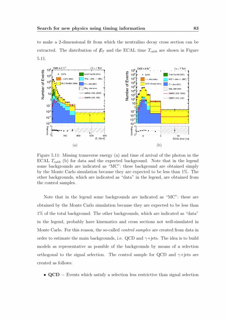
Search for new physics using timing information 83
to make a 2-dimensional fit from which the neutralino decay cross section can be
extracted. The distribution of 6ET and the ECAL time Tcalib are shown in Figure
5.11.
(a) (b)
Figure 5.11: Missing transverse energy (a) and time of arrival of the photon in theECAL Tcalib (b) for data and the expected background. Note that in the legendsome backgrounds are indicated as “MC”: these background are obtained simplyby the Monte Carlo simulation because they are expected to be less than 1%. Theother backgrounds, which are indicated as “data” in the legend, are obtained fromthe control samples.
Note that in the legend some backgrounds are indicated as “MC”: these are
obtained by the Monte Carlo simulation because they are expected to be less than
1% of the total background. The other backgrounds, which are indicated as “data”
in the legend, probably have kinematics and cross sections not well-simulated in
Monte Carlo. For this reason, the so-called control samples are created from data in
order to estimate the main backgrounds, i.e. QCD and γ+jets. The idea is to build
models as representative as possible of the backgrounds by means of a selection
orthogonal to the signal selection. The control sample for QCD and γ+jets are
created as follows:
• QCD − Events which satisfy a selection less restrictive than signal selection
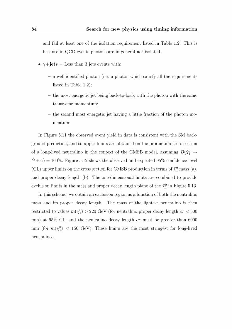
84 Search for new physics using timing information
and fail at least one of the isolation requirement listed in Table 1.2. This is
because in QCD events photons are in general not isolated.
• γ+jets − Less than 3 jets events with:
– a well-identified photon (i.e. a photon which satisfy all the requirements
listed in Table 1.2);
– the most energetic jet being back-to-back with the photon with the same
transverse momentum;
– the second most energetic jet having a little fraction of the photon mo-
mentum;
In Figure 5.11 the observed event yield in data is consistent with the SM back-
ground prediction, and so upper limits are obtained on the production cross section
of a long-lived neutralino in the context of the GMSB model, assuming B(χ01 →
G+ γ) = 100%. Figure 5.12 shows the observed and expected 95% confidence level
(CL) upper limits on the cross section for GMSB production in terms of χ01 mass (a),
and proper decay length (b). The one-dimensional limits are combined to provide
exclusion limits in the mass and proper decay length plane of the χ01 in Figure 5.13.
In this scheme, we obtain an exclusion region as a function of both the neutralino
mass and its proper decay length. The mass of the lightest neutralino is then
restricted to values m(χ01) > 220 GeV (for neutralino proper decay length cτ < 500
mm) at 95% CL, and the neutralino decay length cτ must be greater than 6000
mm (for m(χ01) < 150 GeV). These limits are the most stringest for long-lived
neutralinos.
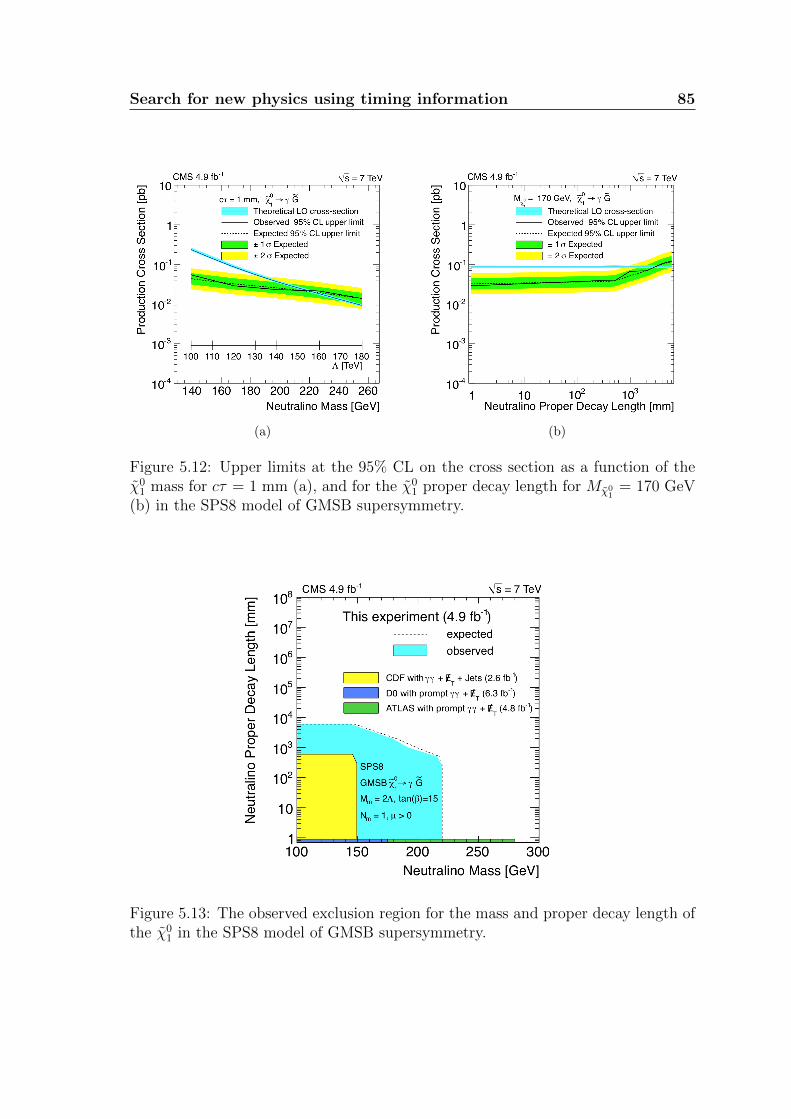
Search for new physics using timing information 85
(a) (b)
Figure 5.12: Upper limits at the 95% CL on the cross section as a function of theχ01 mass for cτ = 1 mm (a), and for the χ0
1 proper decay length for Mχ01
= 170 GeV(b) in the SPS8 model of GMSB supersymmetry.
Figure 5.13: The observed exclusion region for the mass and proper decay length ofthe χ0
1 in the SPS8 model of GMSB supersymmetry.

Conclusions
In this thesis the performance of the timing reconstruction with the CMS electromag-
netic calorimeter (ECAL) has been studied. The ECAL is a hermetic calorimeter
made of lead tungstate (PbWO4) crystals and the combination of the scintillation
timescale of the PbWO4, the electronic pulse shaping and the sampling rate provide
an excellent time resolution. High momentum photons and electrons events from pp
collisions at√s = 7 TeV have been used for this purpose.
The first part of the study was devoted to validate the time resolution measure-
ments obtained prior to LHC collisions. Using samples of reconstructed photons
the energy dependence of the resolution has been extracted. The noise term, pro-
portional to 1/E, came out similar to previous studies on data, although there is a
small difference which is probably due to a different hardware confirguration. The
constant term is confirmed to be of the order of 200 ps.
The second part was about the study of the time development of the electromag-
netic showers. This is possible since for large photon energies (> 20 GeV) the time
can be measured with better than 1 ns resolution in many crystals involved by the
shower. Given that the size of the crystals is about 20 cm×3 cm×3 cm, delays of a
fraction of ns are expected in outlying crystals. A clear dependence of the measured
time as a function of the distance from the impact position has been observed. This
time dependance has been also exploited to implement a discriminant variable for
photon identification purposes. Results are encouraging and this new variable could
be used to further improve the photon-jet separation in physics analyses.
In the third part, a novel method to determine the position of the primary
88 Conclusions
vertex using timing information has been also developed. This method is completely
independent of the tracking, and may offer an important alternative to reject noise
from pileup and to handle in events where there is a small track activity, such as
H → γγ events. A resolution on the vertex position along z axis of about 10 cm
and about 5 cm has been obtained in data and Monte Carlo, respectively. The
method is not yet usable but if an improved time calibration (< 50 ps) will be
reached, O(1cm) resolutions may be obtained. Such a result, if achieved, would give
an important additional ingredient for the H → γγ analysis to better determine the
vertex position. These studies can also guide some of the ongoing feasibility studies
aimed to design the upgrade of the ECAL detector.
Finally, the search for long-lived particles has been presented. It is the first
publication of CMS which makes use of the ECAL timing information [14]. This
analysis has been focused on the SUSY theories with GMSB, where the neutralino
is the Next to Lightest Supersymmetric Particle (NLSP) decaying into a photon
and a gravitino G. In this model, G play the role of the Lightest Supersymmetric
Particle (LSP) and behaves as a massive neutrino, since it is stable, neutral and
weakly interacting. The analysis has used the missing transverse energy and the
ECAL timing to search for an excess of events over the SM background prediction.
A fit to the 2-dimensional distribution in these variables yields no significant excess
of events beyond the SM contributions, and upper limits at 95% are obtained on
the GMSB production cross section in the SPS8 model of GMSB supersymmetry.
Moreover, we obtain an exclusion region as a function of both the neutralino mass
and its proper decay length. The mass of the lightest neutralino is then restricted
to values m(χ01) > 220 GeV (for neutralino proper decay length cτ < 500 mm) at
95% CL, and the neutralino decay length cτ must be greater than 6000 mm (for
m(χ01) < 150 GeV). These limits are the most stringest for long-lived neutralinos.
Ringraziamenti
La lista delle persone da ringraziare e davvero lunga e sono costretta a sfoltirla.
Spero, tuttavia, che ognuna delle persone incontrate in questi miei sei anni di studi
sappia che ha contribuito a farmi giungere a questo traguardo.
Tra le persone che hanno avuto piu peso in questo passo finale, ringrazio in
primis il Dr. Daniele Del Re, ottimo relatore, sempre disponibile e soprattutto
paziente. Ho apprezzato molto quando, insieme al Prof. Luciano M. Barone, mi ha
offerto comprensione in un momento difficile della mia vita e per avermi risollevato
permettendomi di realizzare un lavoro di tesi davvero bello ed interessante.
Ringrazio tutta la ciurma di CMS Roma, dai ricercatori e professori, che mi
hanno ascoltato nelle riunioni e mi hanno offerto critiche costruttive e consigli per
migliorare, agli abitanti della baita, che hanno reso le giornate di duro lavoro piacevoli
e divertenti e mi hanno affiancato nell’eterna battaglia contro Root (consolandomi
quando quest’ultimo mi derideva con qualche “Break violation”). Ed un grazie
speciale va a Livia, capa, mentore ed amica: senza il suo aiuto questa tesi non
sarebbe stata semplice, sia a livello tecnico che emotivo. L’amicizia nata tra noi
durante questo periodo ha impreziosito notevolmente questa esperienza ed io ne ho
fatto tesoro.
Ringrazio i miei amici delle pause pranzo e delle pause Simone trascorse sul
pratino davanti al VEF e sul balcone del primo piano: quei momenti di relax fatti di
risate e non-sense mi rimettevano al mondo. Ed un grazie particolare va ad Andrea,
che grazie allo scambio via Skype di spezzoni tratti dai film di Bud Spencer e Terence
Hill, ha dato una marcia in piu al mio lavoro.
90 Ringraziamenti
Un grazie davvero speciale e per i miei amici piu stretti, Nicolo, Alex e le Ninja
girls : spero siano consapevoli di quanto sia stato fondamentale per me averli avuti
vicino nell’ultimo anno.
Un po’ piu di striscio in questa tesi, ma pur sempre fondamentali nel fortificare
la mia autostima, sono stati i mitici Arnulf Boys, di cui gelosamente conservo la
maglietta di appartenenza. Quelle due settimane insieme a loro sono state un sogno
che mi ha dato un’ulteriore conferma del piacere di essere un fisico.
Ringrazio, poi, la mia famiglia: il Babbo per il suo affetto sconfinato; i miei nonni
per le perle di saggezza e gli aneddoti divertenti; Maurizio per il suo chiamarmi Sette
facendomi sentire un genietto; la Mommo per i suoi consigli e la pazienza in risposta
ai miei scatti di nervi; i bimbi della casa, ossia Pepo, Stella e Luna, per la serenita
e la tenerezza che portano nel mio cuore.
Infine, per ultimi ma non ultimi, ringrazio il mio fratellone Mattia, mio eroe e
modello da imitare, che non ha mai smesso di aver fiducia nella sua sorellina tutta
pepe; ed il mio ragazzo Andrea, dolce e premuroso che, nonostante la nostra sia una
relazione a distanza, mi e sempre stato vicino.
E con questa tesi chiudo il mio capitolo di vita romana.
Una nuova avventura in qualche altro posto mi attende.
Allons-y! (cit. The Tenth Doctor)
Bibliography
[1] Lyndon Evans, “The CERN Large Hadron Collider: Accelerator and Experi-
ments - LHC Machine”, JINST 3 (2008) S08001
LHC/LHCmachine/2008 JINST 3 S08001.
[2] The CMS Collaboration, “The CERN Large Hadron Collider: Accelerator and
Experiments - The CMS experiment at the CERN LHC”, JINST 3 (2008) S08004
LHC/CMS/2008 JINST 3 S08004.
[3] The CMS Collaboration, “CMS Physics Technical Design Report Volume I: De-
tector Performance and Software”, CERN-LHCC-2006-001; CMS-TDR-008-1
cds.cern.ch/record/922757.
[4] The CMS Collaboration, “Electromagnetic calorimeter calibration with 7 TeV
data”, CMS PAS EGM-10-003
cds.cern.ch/record/1279350
[5] The CMS Collaboration, “Time Reconstruction and Performance of the CMS
Electromagnetic Calorimeter”, CMS-CFT-09-006
arXiv:hep-ph/9801271.
[6] T. Sjostrand, S. Mrenna, and P. Z. Skands, “Pythia 6.4 physics and manual”,
JHEP 05:026 (2006)
arXiv:hep-ph/0603175.
92 BIBLIOGRAPHY
[7] J. Alwall et al., “MadGraph 5: Going Beyond”, JHEP 06:128 (2011)
arXiv:hep-ph/1106.0522.
[8] J. Pumplin et al., “New generation of parton distributions with uncertainties
from global QCD analysis”, JHEP 0207:012 (2002)
arXiv:hep-ph/0201195.
[9] GEANT4 Collaboration, “GEANT4 − a simulation toolkit”, Nucl. Instrum.
Meth. A 506 (2003) 250-303
doi:10.1016/S0168-9002(03)01368-8.
[10] The CMS Collaboration, “Search for new physics with long-lived particles de-
caying to photons and missing energy in pp collisions at√s = 7 TeV”, CMS-
EXO-11-067; CERN-PH-EP-2012-164
arXiv:hep-ex/1207.0627
[11] Wolfram Erdmann, “Vertex reconstruction at the CMS experiment”, J. Phys.:
Conf. Ser. 110 092009 (2008)
doi:10.1088/1742-6596/110/9/092009.
[12] The CMS Collaboration, “Tracking and vertexing performance in CMS”, CMS
CR -2012/384.
[13] The CMS Collaboration, “Search for the standard model Higgs boson decaying
into two photons in pp collisions at√s = 7 TeV”, Phys. Lett. B 710 (2012) 403;
CMS-HIG-11-033; CERN-PH-EP-2012-024
arXiv:hep-ex/1202.1487.
[14] The CMS Collaboration, “Search for long-lived particles decaying to photons
and missing energy in proton-proton collisions at√s = 7 TeV”, Phys. Lett. B ;
CMS-EXO-11-035; CERN-PH-EP-2012-342
arXiv:hep-ex/1212.1838.
BIBLIOGRAPHY 93
[15] W. Hollik, “Quantum field theory and the Standard Model”, CERN Yellow
Report CERN-2010-002 pp.1-44
arXiv:hep-ph/1012.3883.
[16] P. W. Higgs, “Broken symmetries, massless particles and gauge fields”, Phys.
Lett. 12 (2) 132–201 (1964)
doi:10.1016/0031-9163(64)91136-9.
[17] P. W. Higgs, “Broken Symmetries and the Masses of Gauge Bosons”, Phys.
Rev. Lett. 13 (16) 508 (1964)
doi:10.1103/PhysRevLett.13.508.
[18] S. P. Martin, “A Supersymmetry Primer”
arXiv:hep-ph/9709356.
[19] Matthew J. Strassler, Kathryn M. Zurek, “Echoes of a Hidden Valley at Hadron
Colliders”, Phys. Lett. B651 (2007) 374
arXiv:hep-ph/0604261.
[20] D. I. Kazakov, “Beyond the Standard Model”
arXiv:hep-ph/0411064
[21] G. F. Giudice and R. Rattazzi, “Theories with gauge-mediated supersymmetry
breaking”, Phys. Rept. 322 (1999) 419
arXiv:hep-ph/9801271.
[22] G. R. Farrar and P. Fayet, “Phenomenology of the Production, Decay, and
Detection of New Hadronic States Associated with Supersymmetry”, Phys. Lett.
B76 (1978) 575-579
doi:10.1016/0370-2693(78)90858-4.