Fast Elliptic Curve Cryptography Using Minimal …crpit.com/confpapers/CRPITV125Suppakitpaisarn.pdfFast Elliptic Curve Cryptography Using Minimal Weight Conversion of d Integers Vorapong

Fast Elliptic Curve Cryptography Using

Minimal Weight Conversion of d Integers

Vorapong Suppakitpaisarn1 Masato Edahiro2 Hiroshi Imai1

1 Department of Computer Science, Graduate School of Information Science and TechnologyThe University of Tokyo,

Hongo, Bunkyo-ku, Tokyo, 113-8656Email: mr t [email protected], [email protected]

2 Department of Information Engineering, Graduate School of Information ScienceNagoya University,

Furo-cho, Chikusa-ku, Nagoya-shi, Aichi 464-8601Email: [email protected]

Abstract

In this paper, we reduce computation time of ellip-tic curve signature verification scheme by proposingthe minimal joint Hamming weight conversion forany binary expansions of d integers. The computa-tion time of multi-scalar multiplication, the bottle-neck operation of the scheme, strongly depends on thejoint Hamming weight. As we represent the scalarsusing redundant representations, we may representa number by many expansions. The minimal jointHamming weight conversion is the algorithm to se-lect the expansion which has the least joint Hammingweight. Many existing works introduce the conver-sions for some specific representations, and it is nottrivial to generalize their algorithms to other repre-sentations. On the other hand, our conversion, basedon the dynamic programming scheme, is applicable tofind the optimal expansions on any binary represen-tations. We also propose the algorithm to generatethe Markov chain used for exploring the minimal av-erage Hamming density automatically from our con-version algorithm. In general, the sets of states inour Markov chains are infinite. Then, we introducea technique to reduce the number of Markov chainstates to a finite set. With the technique, we find theaverage joint Hamming weight of many representa-tions that have never been found. One of the mostsignificant results is that, for the expansion of inte-ger pairs when the digit set is {0,±1,±3} often usedin multi-scalar multiplication, we show that the min-imal average joint Hamming density is 0.3575, whichimproves the upper bound value.

Keywords: Elliptic Curve Cryptography, MinimalWeight Conversion, Average Joint Hamming Weight,Digit Set Expansion

1 Introduction

The multi-scalar multiplication is the bottleneck op-eration of elliptic curve signature verification scheme.

Copyright c©2012, Australian Computer Society, Inc. Thispaper appeared at the 10th Australasian Information Secu-rity Conference (AISC 2012), Melbourne, Australia, January-February 2012. Conferences in Research and Practice in In-formation Technology (CRPIT), Vol. 125, Josef Pieprzyk andClark Thomborson, Ed. Reproduction for academic, not-for-profit purposes permitted provided this text is included.

The operation is to compute

K =

d∑

i=1

riPi = r1P1 + · · ·+ rdPd,

when ri is a natural number, and Pi is a pointon the elliptic curve. In this paper, we propose amethod to reduce the computation time using a com-puter arithmetic technique considering the represen-tation of each scalar ri. In some redundant repre-sentations, we can represent each ri in more thanone way. Each way, called expansion, has a differ-ent value of Hamming weight, which directly affectsthe computation time of multi-scalar multiplications.Since the lower weight expansion makes the opera-tion faster, many methods have been explored thelower weight expansion on many specific representa-tions (1, 2, 3, 4, 5, 6, 7). These include the work bySolinas (1), which proposed the minimal joint weightexpansion on an integer pair when digit set (definedin Section 2) is {0,±1}. Also, the work by Heubergerand Muir (2, 3) presented the expansions for digit set{−l,−(l−1), . . . ,−1, 0, 1, . . . , u−1, u} for any naturalnumber l, and positive integer u.

However, minimal weight conversions of manydigit sets have not yet been found in the literature.This is caused by the fact that most of previous workpresented the conversions based on the mathematicalconstruction of the representation, which is hard toapply to many types of digit sets.

In this work, we propose a conversion method andan algorithm to find the average weight without con-cerning mathematical construction. This enables usto find the minimal weight conversions of digit setsused for multi-scalar multiplication. One of the signif-icant result is the minimal weight conversion when thedigit set is {0,±1,±3} (8). Compared to the digit setthat the minimal weight conversion have been foundsuch as {0,±1± 2} (2, 3), {0,±1,±3} uses the sameamount of memory to store the pre-computed pointsas {0,±1,±2}, but it is proved that {0,±1,±3} haslower minimal average weight when d = 2.

To evaluate the effectiveness of each representationon elliptic curve cryptography, we utilize the averagejoint Hamming density, and we also propose a methodto find the value for a class of digit set in this pa-per. Similar to the minimal weight conversions, mostof the existing works proposed analysis based on themathematical construction, which makes it hard toapply to many digit sets. On the other hand, we areable to calculate the value for our minimal weight con-

Proceedings of the Tenth Australasian Information Security Conference (AISC 2012), Melbourne, Australia

15

version algorithms, by proposing an algorithm to au-tomatically generate the Markov chain from the con-version algorithms. In general, the sets of states inour Markov chains are infinite. Then, we introducea technique to reduce the number of Markov chainstates to a finite set.

One of our results is the expansion when thedigit set is {0,±1,±3} and d = 2. For this digitset, many previous works have proposed conversionmethods and analysis for multi-scalar multiplication(5, 9, 10, 11). They can find the upper bound for theminimal average joint Hamming density. Our algo-rithm can find the minimal average joint Hammingdensity for this digit set, which is 0.3575. This im-proves the lowest upper bound 0.3616 in (5, 6).

It is shown in Appendix C that our minimal weightconversion algorithm is applicable to all finite digitsets. However, the algorithm to find average jointHamming density is not. In many digit sets, thenumber of states in the Markov chain in the Markovchain is not finite, e.g. the representation in whichDS = {0, 1, 3} and d = 1. In (12), we provide theproof of the finiteness of the Markov chain in a class ofrepresentation which cover all representations practi-cally used in multi-scalar multiplication. Also, we areworking on finding other reduction methods, whichenable us to discover the value for wider class of rep-resentations.

The remainder of this paper is organized as fol-lows: We discuss the background knowledge of thisresearch in Section 2. In Section 3, we propose aminimal weight conversion algorithm, with the expla-nation and the example. In Section 4, we present thealgorithm to construct the Markov chain used for an-alyzing the digit set expansion from the conversionin Section 3. Then, we use that Markov chain to findthe minimal average joint Hamming density. Last, weconclude the paper in Section 5.

2 Definition

Let DS be the digit set, n, d be positive integers,E{DS , d} be a conversion function from Zd to (Dn

S)d

such that if

E{DS , d}(r1, . . . , rd) = 〈(ei,n−1 ei,n−2 . . . e1,0)〉di=1

= 〈(ei,t)n−1t=0 〉

di=1,

when∑n−1

t=0 ei,t2t = ri, where ri ∈ Z and ei,t ∈ DS for

all 1 ≤ i ≤ d. We call 〈(ei,t)n−1t=0 〉

di=1 as the expansion

of r1, . . . , rd by the conversion E{DS, d}. We alsodefine a tuple of t-th bit of ri as,

E{DS , d}(r1, . . . , rd)|t = 〈e1,t, . . . , ed,t〉.

As a special case, let Eb{d} be the binary conver-sion changing the integer to its binary representationwhere DS = {0, 1}.

Eb{1}(12) = 〈(1100)〉,

Eb{2}(12, 21) = 〈(01100), (10101)〉.

Also, define Rt as

Rt = Eb{d}(r1, . . . , rd)|t = 〈e1,t, . . . , ed,t〉

. In our minimal weight conversion, Rt is consideredas the input of bit t.

Next, we define JWE{DS ,d}(r1, . . . , rd), the jointHamming weight function of integer r1, . . . rd repre-sented by the conversion E{DS, d}, by

JWE{DS ,d}(r1, . . . , rd) =n−1∑

t=0

jwt,

where

jwt =

{

0, if E{DS , d}(r1, . . . , rd)|t = 〈0〉,1 otherwise ,

For instance,

JWEb{1}(12) = 2,

JWEb{2}(12, 21) = 4.

The computation time of the scalar point multipli-cation depends on the joint Hamming weight. This isbecause we deploy the double-and-add method, thatis

d∑

i=0

riPi = 2(. . . (2(2Kn−1 + Kn−2)) . . . ) + K0,

where

Kt =

d∑

i=0

ei,tPi.

Since Kt = O, if

E{DS , d}(r1, . . . , rd)|t = 〈0〉,

we need not to perform point addition in thatcase. Thus, the number of point additions isJWE{DS ,d}(r1, . . . , rd)− 1. For instance, if

K = 12P1 + 21P2,

we can compute K as

K = 2(2(2(2P2 + P1) + D)) + P2,

where D = P1 + P2, that has already been precom-puted before the computation begins. We need 4point doubles and 3 point additions to find the re-sult.

When {0, 1} ⊂ DS , we are able to represent somenumber ri ∈ Z in more than one way. For instance,if DS = {0,±1},

12 = (01100) = (101̄00) = (11̄100) = . . . ,

when 1̄ = −1.Let Em{DS, d} be a minimal weight conversion

where

Em{DS, d}(r1, . . . , rd) = 〈(ei,n−1 . . . ei,0)〉di=1

is the expansion such that for any 〈(e′i,n−1 . . . e′i,0)〉ti=1

where∑n−1

t=0 ei,t2t =

∑n−1t=0 e′i,t2

t, for all 1 ≤ i ≤ d,

n−1∑

t=0

jw′t ≥ JWEm{DS ,d}(r1, . . . , rd),

and

CRPIT Volume 125 - Information Security 2012

16

jw′t =

{

0 if 〈e′1,t, . . . , e′d,t〉 = 〈0〉,

1 otherwise .

For instance,

Em{{0,±1}, 2}(12, 21) = 〈(101̄00), (10101)〉,

JWEm{{0,±1},2}(12, 21) = 3.

Then, the number of point additions needed is 2.Also, we call Em{DS , d}(r1, . . . , rd) as the minimalweight expansion of r1, . . . , rd using the digit set DS .

If DS2⊆ DS1

, it is obvious that

JWEm{DS2,d}(r1, . . . , rd) ≥ JWEm{DS1

,d}(r1, . . . , rd).

Thus, we can increase the efficiency of the scalar-point multiplication by increaseing the size of DS .However, the bigger DS needs more precomputationtasks. If d = 2, we need one precomputed point whenDS = {0, 1}, but we need 10 precomputed pointswhen DS = {0,±1,±3}.

Then, one of the contributions of this paper is toevaluate an efficiency of each digit set DS on multi-scalar multiplication. We use the average joint Ham-ming density defined as

AJW (E{DS , d}) =

limn→∞

2n−1∑

r1=0

· · ·

2n−1∑

rd=0

JWE{DS ,d}(r1, . . . , rd)

n2dn.

It is easy to see that AJW (Eb{d}) = 1− 12d . In this

paper, we find the value AJW (Em{DS, d}) of someDS and d. Some of these values have been found inthe literature such as

AJW (Em{{0,±1,±3, . . . ,±(2p−1)}, 1}) =1

p + 1(4).

Also,

AJW (Em{{−l,−(l− 1), . . . ,−1, 0, 1, u− 1, u}, d})

for any positive number d,u, and natural number l,have been found by Heuberger and Muir (2, 3).

3 Minimal Weight Conversion

In this section, we propose a minimal weight conver-sion algorithm based on the dynamic programmingscheme. The input is 〈r1, . . . , rd〉, and the output isEm{DS, d}(r1, . . . , rd), which is the minimal weightexpansion of the input using the digit set DS . Thealgorithm begins from the most significant bit (bitn − 1), Rn−1, and processes left-to-right to the leastsignificant bit (bit 0), R0.

For each t (n > t ≥ 0), we calculate minimalweight expansions of the first n − t bits of the in-put r1, . . . , rd (

⌊

r1

2t

⌋

, . . . ,⌊

rd

2t

⌋

) for all possible carryGt defined below. We state some notations in ouralgorithm as follows:

• The carry array Gt = 〈g1,t, . . . , gd,t〉 is a possibleinteger array as carry from bit t − 1. For theinput

Rt = 〈e1,t, . . . , ed,t〉

and output

R∗t = 〈e∗1,t, . . . , e

∗d,t〉 ∈ Dd

S ,

the following formula should be satisfied:

Rt + Gt = R∗t + 2Gt+1.

Since R∗t ∈ Dd

S , possible values of gi,t is cal-culated from DS. We define the carry set CS

by the set of possible carry values for DS . InAppendix B, we give the detail of the carryset CS , and prove that the set is always finiteif DS is finite. For example, when the digitset DS = {0,±1,±3}, the carry set is CS ={0,±1,±2,±3}. It is noted that Gt = 〈0〉 fort = 0 and t = n as boundary conditions.

• The minimal weight array wt is the array of thepositive integer wt,Gt

for any Gt ∈ CdS . The inte-

ger wt,Gtis the minimal joint weight of the first

n− t bits of the input r1, . . . , rd (⌊

r1

2t

⌋

, . . . ,⌊

rd

2t

⌋

)

for carry Gt = 〈gi,t〉di=1, e.g.

wt,Gt= JWEm{DS ,d}(

⌊r1

2t

⌋

+g1,t, . . . ,⌊rd

2t

⌋

+gd,t).

• The subsolution array Qt is the array of thestring Qt,〈i,Gt〉 for any 1 ≤ i ≤ d and Gt ∈

CdS . Each Qt,〈i,Gt〉 represents the minimal weight

expansion of the first n − t bits of the inputr1, . . . , rd when we carry Gt = 〈gi,t〉

di=1, e.g.

Qt,Gt= 〈Qt,〈i,Gt〉〉

di=1 =

Em{DS, d}(⌊r1

2t

⌋

+ g1,t, . . . ,⌊rd

2t

⌋

+ gd,t).

We note that the length of the string Qt,〈i,Gt〉

is n− t, and wt,Gtis the joint Hamming weight

of the string Qt,〈1,Gt〉, . . . , Qt,〈d,Gt〉. There may

exist some gi,t ∈ CS such that⌊

r1

2t

⌋

+gi,t can notbe represented using the string length n − t ofDS. In that case, we represent Qt,〈i,Gt〉 with thenull string, and assign wt,Gt

to ∞.

In the process at the bit t, we find the minimalweight array wt and the subsolution array Qt fromthe input Rt, the minimal weight array wt+1, and thesubsolution array Qt+1. For the process, we definethe function MW such that

(wt,Gt, Qt,Gt

) = MW (wt+1, Qt+1, Rt, Gt).

Since wt = 〈wt,Gt〉Gt∈Cd

Sand Qt = 〈Qt,Gt

〉Gt∈CdS, we

also define

(wt, Qt) = MW (wt+1, Qt+1, Rt).

It is important to note that wt is only depend onwt+1 and Rt, and we can use only two arrays to repre-sent all wt and wt+1 to reduce memory consumption.Similarly, we store all Qt using two arrays.

Here, we will show the basic idea of our proposedalgorithm with an example.

Example 1 Compute the minimal weight expan-sion of 3 and 7 when the digit set is {0,±1,±3},Em{{0,±1,±3}, 2}(3, 7). Note that the binary rep-resentation Eb{2}(3, 7) = 〈(011), (111)〉.

• Step 1 Consider the most significant bit, the in-put

R2 = Eb{2}(3, 7)|t=2 = 〈0, 1〉.


17

For the digit set DS = {0,±1,±3}, the carryset is calculated as CS = {0,±1,±2,±3}. Thus,there are 25 pairs for possible carries G2. Forexample, when G2 = 〈0,−1〉, R2 + G2 = 〈0, 1〉+〈0,−1〉 = 〈0, 0〉, so that the Hamming weightw2,〈0,−1〉 = 0. As a boundary condition, we donot generate carry from the most significant bitbecause we want to keep the length of the bitstring unchanged.

If G2 = 〈1, 0〉, the input with the carry,

R2 + G2 = 〈0, 1〉+ 〈1, 0〉 = 〈1, 1〉,

and w2,〈1,0〉 = 1. The Hamming weight w2,G2is

1 for any G, such that

R2 + G2 ∈ DdS − {〈0〉}.

If G2 = 〈0, 1〉,

R2 + G2 = 〈0, 1〉+ 〈0, 1〉 = 〈0, 2〉,

and w2,〈0,1〉 = ∞, because 2 is not in DS . TheHamming weight w2,G is∞ for any G2, such thatR2 + G2 /∈ Dd

S .

• Step 2 Next, we consider bit 1. In this bit,

R1 = Eb{2}(3, 7)|t=1 = 〈1, 1〉.

Consider the case when the carry from the leastsignificant bit G1 = 〈1, 0〉. Then, R1 + G1 =〈2, 1〉. There are 4 ways to write 〈2, 1〉 in theform 2Gt+1 + R∗

t where Gt+1 ∈ CdS is the carry

to the most significant bit and R∗t ∈ Dd

S is thecandidate for the output. That is

〈2, 1〉 = 2× 〈1, 0〉+ 〈0, 1〉

= 2× 〈1,−1〉+ 〈0, 3〉

= 2× 〈1, 1〉+ 〈0,−1〉

= 2× 〈1, 2〉+ 〈0,−3〉.

The Hamming weight should be

wt,Gt= min

Gt+1,R∗

t

[wt+1,Gt+1+ JW (R∗

t )].

From the calculation for bit 2 shown in Page 3,

w2,〈1,0〉 = w2,〈1,−1〉 = w2,〈1,2〉 = 1,

w2,〈1,1〉 =∞.

And,

JW (〈1, 0〉) = JW (〈0, 3〉)

= JW (〈0,−1〉)

= JW (〈0,−3〉)

= 1.

Then,

w1,〈1,0〉 = minG2,R∗

t

[w2,G2+ JW (R∗

1)] = 1 + 1 = 2.

We show the array w1,G1on this bit in Table 1.

• Step 3 On the least significant bit, the inputR0 = 〈1, 1〉. Also, as a boundary condition, weset G0 = 〈0〉, and therefore, the value w0,〈0,0〉

is the minimal Hamming weight. When G0 =〈0, 0〉, R0 + G0 = 〈1, 1〉. Similar to bit 1, we find

w0,〈0,0〉 = minG1,R∗

0

[w1,G1+ JW (R∗

0)],

such that 2×G1+R∗0 = 〈1, 1〉, and G1 ∈ Cd

S , R∗0 ∈

DdS. We show the value of each possible G1, R

∗0

with w1,G1, JW (R∗

0), and w1,G1+JW (R∗

0) in Ta-ble 2. Shown in the table, the minimal Hammingweight is

minG1,R∗

0

[w1,G1+ JW (R∗

0)] = 2.

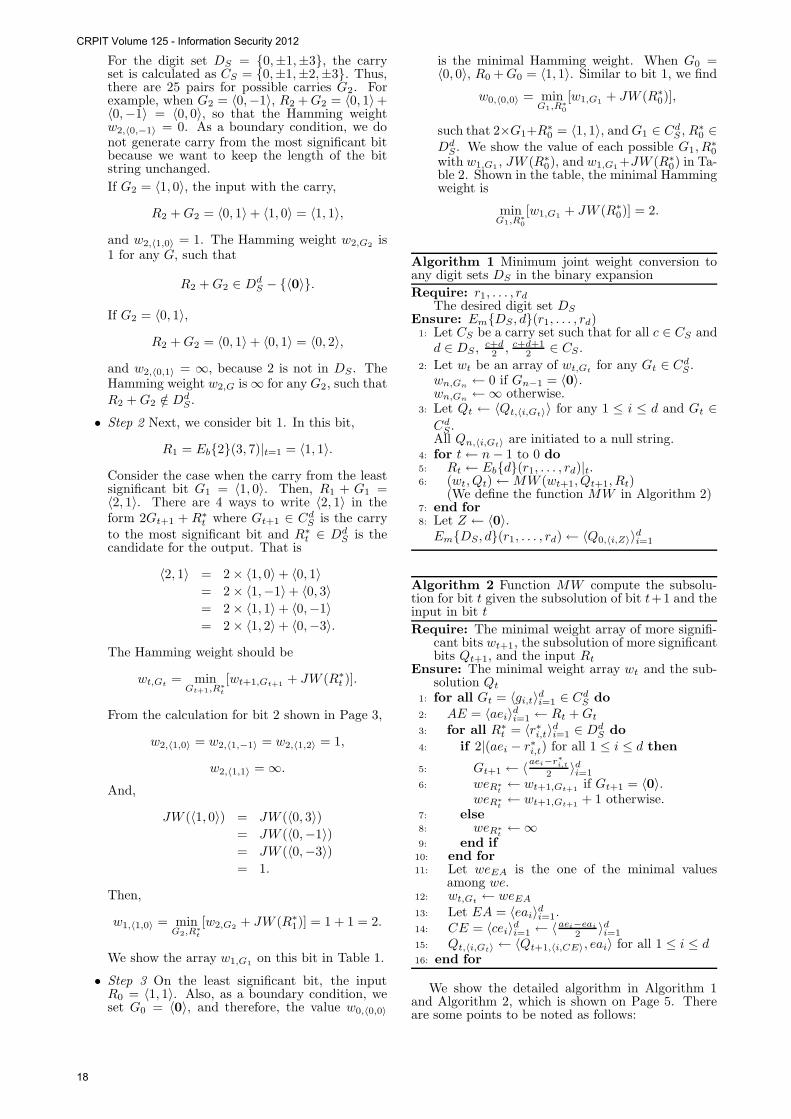
Algorithm 1 Minimum joint weight conversion toany digit sets DS in the binary expansion

Require: r1, . . . , rd

The desired digit set DS

Ensure: Em{DS, d}(r1, . . . , rd)1: Let CS be a carry set such that for all c ∈ CS and

d ∈ DS , c+d2 , c+d+1

2 ∈ CS .

2: Let wt be an array of wt,Gtfor any Gt ∈ Cd

S .wn,Gn

← 0 if Gn−1 = 〈0〉.wn,Gn

←∞ otherwise.3: Let Qt ← 〈Qt,〈i,Gt〉〉 for any 1 ≤ i ≤ d and Gt ∈

CdS .

All Qn,〈i,Gt〉 are initiated to a null string.4: for t← n− 1 to 0 do5: Rt ← Eb{d}(r1, . . . , rd)|t.6: (wt, Qt)←MW (wt+1, Qt+1, Rt)

(We define the function MW in Algorithm 2)7: end for8: Let Z ← 〈0〉.

Em{DS, d}(r1, . . . , rd)← 〈Q0,〈i,Z〉〉di=1

Algorithm 2 Function MW compute the subsolu-tion for bit t given the subsolution of bit t+1 and theinput in bit t

Require: The minimal weight array of more signifi-cant bits wt+1, the subsolution of more significantbits Qt+1, and the input Rt

Ensure: The minimal weight array wt and the sub-solution Qt

1: for all Gt = 〈gi,t〉di=1 ∈ Cd

S do2: AE = 〈aei〉

di=1 ← Rt + Gt

3: for all R∗t = 〈r∗i,t〉

di=1 ∈ Dd

S do4: if 2|(aei − r∗i,t) for all 1 ≤ i ≤ d then

5: Gt+1 ← 〈aei−r∗

i,t

2 〉di=1

6: weR∗

t← wt+1,Gt+1

if Gt+1 = 〈0〉.weR∗

t← wt+1,Gt+1

+ 1 otherwise.7: else8: weR∗

t←∞

9: end if10: end for11: Let weEA is the one of the minimal values

among we.12: wt,Gt

← weEA

13: Let EA = 〈eai〉di=1.

14: CE = 〈cei〉di=1 ← 〈

aei−eai

2 〉di=1

15: Qt,〈i,Gt〉 ← 〈Qt+1,〈i,CE〉, eai〉 for all 1 ≤ i ≤ d16: end for

We show the detailed algorithm in Algorithm 1and Algorithm 2, which is shown on Page 5. Thereare some points to be noted as follows:


18

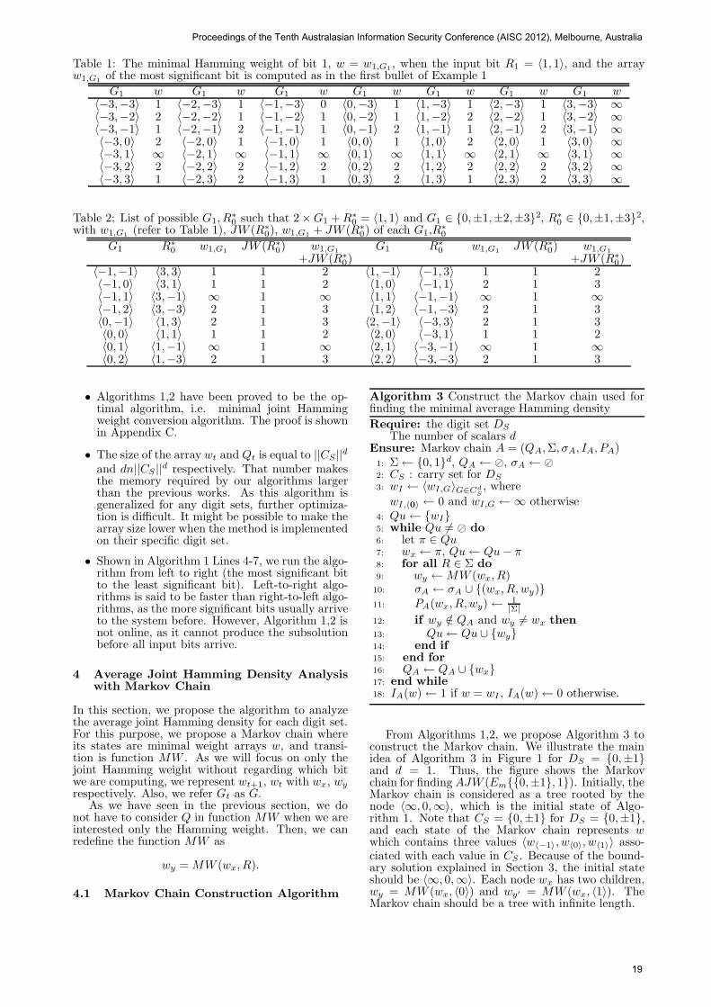
Table 1: The minimal Hamming weight of bit 1, w = w1,G1, when the input bit R1 = 〈1, 1〉, and the array

w1,G1of the most significant bit is computed as in the first bullet of Example 1

G1 w G1 w G1 w G1 w G1 w G1 w G1 w〈−3,−3〉 1 〈−2,−3〉 1 〈−1,−3〉 0 〈0,−3〉 1 〈1,−3〉 1 〈2,−3〉 1 〈3,−3〉 ∞〈−3,−2〉 2 〈−2,−2〉 1 〈−1,−2〉 1 〈0,−2〉 1 〈1,−2〉 2 〈2,−2〉 1 〈3,−2〉 ∞〈−3,−1〉 1 〈−2,−1〉 2 〈−1,−1〉 1 〈0,−1〉 2 〈1,−1〉 1 〈2,−1〉 2 〈3,−1〉 ∞〈−3, 0〉 2 〈−2, 0〉 1 〈−1, 0〉 1 〈0, 0〉 1 〈1, 0〉 2 〈2, 0〉 1 〈3, 0〉 ∞〈−3, 1〉 ∞ 〈−2, 1〉 ∞ 〈−1, 1〉 ∞ 〈0, 1〉 ∞ 〈1, 1〉 ∞ 〈2, 1〉 ∞ 〈3, 1〉 ∞〈−3, 2〉 2 〈−2, 2〉 2 〈−1, 2〉 2 〈0, 2〉 2 〈1, 2〉 2 〈2, 2〉 2 〈3, 2〉 ∞〈−3, 3〉 1 〈−2, 3〉 2 〈−1, 3〉 1 〈0, 3〉 2 〈1, 3〉 1 〈2, 3〉 2 〈3, 3〉 ∞

Table 2: List of possible G1, R∗0 such that 2×G1 + R∗

0 = 〈1, 1〉 and G1 ∈ {0,±1,±2,±3}2, R∗0 ∈ {0,±1,±3}2,

with w1,G1(refer to Table 1), JW (R∗

0), w1,G1+ JW (R∗

0) of each G1,R∗0

G1 R∗0 w1,G1

JW (R∗0) w1,G1

G1 R∗0 w1,G1

JW (R∗0) w1,G1

+JW (R∗0) +JW (R∗

0)〈−1,−1〉〈3, 3〉 1 1 2 〈1,−1〉〈−1, 3〉 1 1 2〈−1, 0〉〈3, 1〉 1 1 2 〈1, 0〉〈−1, 1〉 2 1 3〈−1, 1〉〈3,−1〉 ∞ 1 ∞ 〈1, 1〉〈−1,−1〉 ∞ 1 ∞〈−1, 2〉〈3,−3〉 2 1 3 〈1, 2〉〈−1,−3〉 2 1 3〈0,−1〉〈1, 3〉 2 1 3 〈2,−1〉〈−3, 3〉 2 1 3〈0, 0〉〈1, 1〉 1 1 2 〈2, 0〉〈−3, 1〉 1 1 2〈0, 1〉〈1,−1〉 ∞ 1 ∞ 〈2, 1〉〈−3,−1〉 ∞ 1 ∞〈0, 2〉〈1,−3〉 2 1 3 〈2, 2〉〈−3,−3〉 2 1 3

• Algorithms 1,2 have been proved to be the op-timal algorithm, i.e. minimal joint Hammingweight conversion algorithm. The proof is shownin Appendix C.

• The size of the array wt and Qt is equal to ||CS ||d

and dn||CS ||d respectively. That number makes

the memory required by our algorithms largerthan the previous works. As this algorithm isgeneralized for any digit sets, further optimiza-tion is difficult. It might be possible to make thearray size lower when the method is implementedon their specific digit set.

• Shown in Algorithm 1 Lines 4-7, we run the algo-rithm from left to right (the most significant bitto the least significant bit). Left-to-right algo-rithms is said to be faster than right-to-left algo-rithms, as the more significant bits usually arriveto the system before. However, Algorithm 1,2 isnot online, as it cannot produce the subsolutionbefore all input bits arrive.

4 Average Joint Hamming Density Analysiswith Markov Chain

In this section, we propose the algorithm to analyzethe average joint Hamming density for each digit set.For this purpose, we propose a Markov chain whereits states are minimal weight arrays w, and transi-tion is function MW . As we will focus on only thejoint Hamming weight without regarding which bitwe are computing, we represent wt+1, wt with wx, wy

respectively. Also, we refer Gt as G.As we have seen in the previous section, we do

not have to consider Q in function MW when we areinterested only the Hamming weight. Then, we canredefine the function MW as

wy = MW (wx, R).

4.1 Markov Chain Construction Algorithm

Algorithm 3 Construct the Markov chain used forfinding the minimal average Hamming density

Require: the digit set DS

The number of scalars dEnsure: Markov chain A = (QA, Σ, σA, IA, PA)

1: Σ← {0, 1}d, QA ← �, σA ← �2: CS : carry set for DS

3: wI ← 〈wI,G〉G∈CdS, where

wI,〈0〉 ← 0 and wI,G ←∞ otherwise4: Qu← {wI}5: while Qu 6= � do6: let π ∈ Qu7: wx ← π, Qu← Qu− π8: for all R ∈ Σ do9: wy ←MW (wx, R)

10: σA ← σA ∪ {(wx, R, wy)}11: PA(wx, R, wy)← 1

|Σ|

12: if wy /∈ QA and wy 6= wx then13: Qu← Qu ∪ {wy}14: end if15: end for16: QA ← QA ∪ {wx}17: end while18: IA(w)← 1 if w = wI , IA(w)← 0 otherwise.

From Algorithms 1,2, we propose Algorithm 3 toconstruct the Markov chain. We illustrate the mainidea of Algorithm 3 in Figure 1 for DS = {0,±1}and d = 1. Thus, the figure shows the Markovchain for finding AJW (Em{{0,±1}, 1}). Initially, theMarkov chain is considered as a tree rooted by thenode 〈∞, 0,∞〉, which is the initial state of Algo-rithm 1. Note that CS = {0,±1} for DS = {0,±1},and each state of the Markov chain represents wwhich contains three values 〈w〈−1〉, w〈0〉, w〈1〉〉 asso-ciated with each value in CS . Because of the bound-ary solution explained in Section 3, the initial stateshould be 〈∞, 0,∞〉. Each node wx has two children,wy = MW (wx, 〈0〉) and wy′ = MW (wx, 〈1〉). TheMarkov chain should be a tree with infinite length.


19

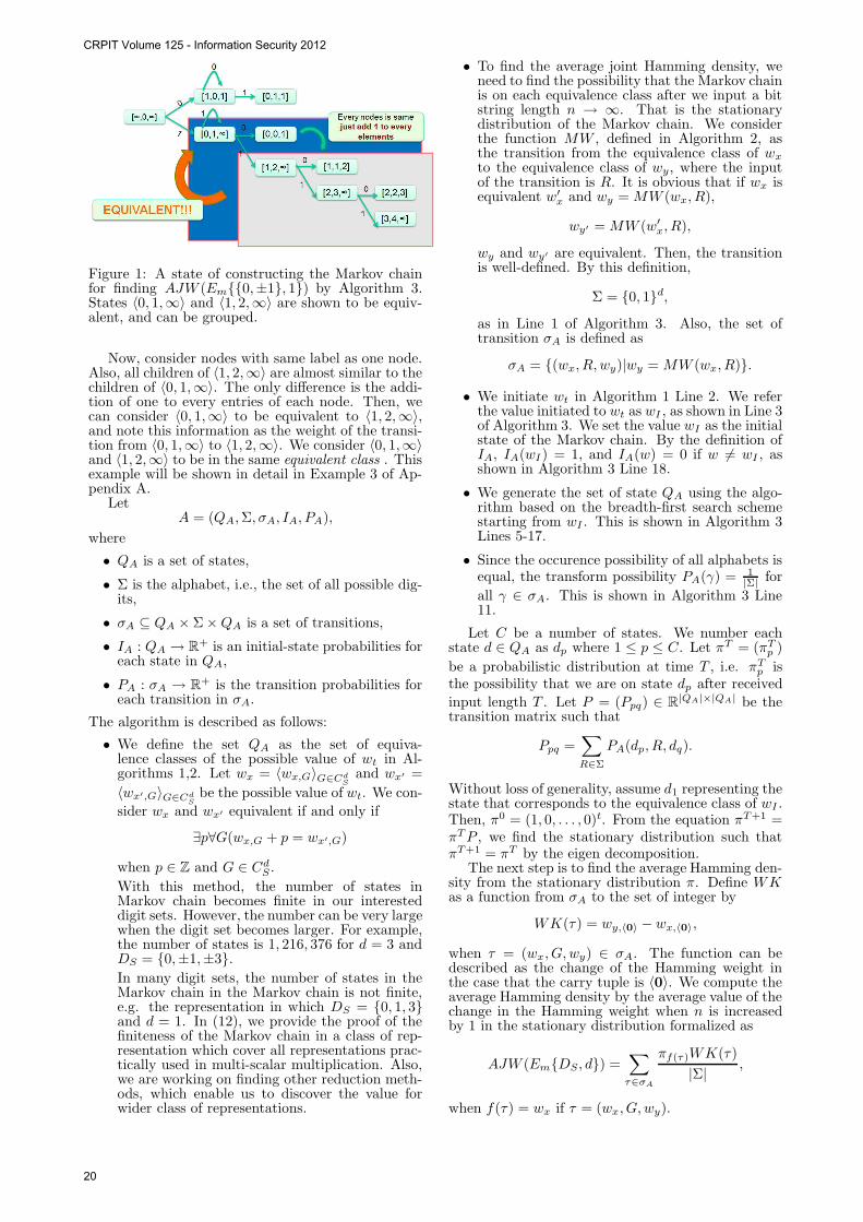
Figure 1: A state of constructing the Markov chainfor finding AJW (Em{{0,±1}, 1}) by Algorithm 3.States 〈0, 1,∞〉 and 〈1, 2,∞〉 are shown to be equiv-alent, and can be grouped.

Now, consider nodes with same label as one node.Also, all children of 〈1, 2,∞〉 are almost similar to thechildren of 〈0, 1,∞〉. The only difference is the addi-tion of one to every entries of each node. Then, wecan consider 〈0, 1,∞〉 to be equivalent to 〈1, 2,∞〉,and note this information as the weight of the transi-tion from 〈0, 1,∞〉 to 〈1, 2,∞〉. We consider 〈0, 1,∞〉and 〈1, 2,∞〉 to be in the same equivalent class . Thisexample will be shown in detail in Example 3 of Ap-pendix A.

LetA = (QA, Σ, σA, IA, PA),

where

• QA is a set of states,

• Σ is the alphabet, i.e., the set of all possible dig-its,

• σA ⊆ QA × Σ×QA is a set of transitions,

• IA : QA → R+ is an initial-state probabilities foreach state in QA,

• PA : σA → R+ is the transition probabilities foreach transition in σA.

The algorithm is described as follows:

• We define the set QA as the set of equiva-lence classes of the possible value of wt in Al-gorithms 1,2. Let wx = 〈wx,G〉G∈Cd

Sand wx′ =

〈wx′,G〉G∈CdS

be the possible value of wt. We con-

sider wx and wx′ equivalent if and only if

∃p∀G(wx,G + p = wx′,G)

when p ∈ Z and G ∈ CdS .

With this method, the number of states inMarkov chain becomes finite in our interesteddigit sets. However, the number can be very largewhen the digit set becomes larger. For example,the number of states is 1, 216, 376 for d = 3 andDS = {0,±1,±3}.

In many digit sets, the number of states in theMarkov chain in the Markov chain is not finite,e.g. the representation in which DS = {0, 1, 3}and d = 1. In (12), we provide the proof of thefiniteness of the Markov chain in a class of rep-resentation which cover all representations prac-tically used in multi-scalar multiplication. Also,we are working on finding other reduction meth-ods, which enable us to discover the value forwider class of representations.

• To find the average joint Hamming density, weneed to find the possibility that the Markov chainis on each equivalence class after we input a bitstring length n → ∞. That is the stationarydistribution of the Markov chain. We considerthe function MW , defined in Algorithm 2, asthe transition from the equivalence class of wx

to the equivalence class of wy, where the inputof the transition is R. It is obvious that if wx isequivalent w′

x and wy = MW (wx, R),

wy′ = MW (w′x, R),

wy and wy′ are equivalent. Then, the transitionis well-defined. By this definition,

Σ = {0, 1}d,

as in Line 1 of Algorithm 3. Also, the set oftransition σA is defined as

σA = {(wx, R, wy)|wy = MW (wx, R)}.

• We initiate wt in Algorithm 1 Line 2. We referthe value initiated to wt as wI , as shown in Line 3of Algorithm 3. We set the value wI as the initialstate of the Markov chain. By the definition ofIA, IA(wI ) = 1, and IA(w) = 0 if w 6= wI , asshown in Algorithm 3 Line 18.

• We generate the set of state QA using the algo-rithm based on the breadth-first search schemestarting from wI . This is shown in Algorithm 3Lines 5-17.

• Since the occurence possibility of all alphabets isequal, the transform possibility PA(γ) = 1

|Σ| for

all γ ∈ σA. This is shown in Algorithm 3 Line11.

Let C be a number of states. We number eachstate d ∈ QA as dp where 1 ≤ p ≤ C. Let πT = (πT

p )

be a probabilistic distribution at time T , i.e. πTp is

the possibility that we are on state dp after received

input length T . Let P = (Ppq) ∈ R|QA|×|QA| be thetransition matrix such that

Ppq =∑

R∈Σ

PA(dp, R, dq).

Without loss of generality, assume d1 representing thestate that corresponds to the equivalence class of wI .Then, π0 = (1, 0, . . . , 0)t. From the equation πT+1 =πT P , we find the stationary distribution such thatπT+1 = πT by the eigen decomposition.

The next step is to find the average Hamming den-sity from the stationary distribution π. Define WKas a function from σA to the set of integer by

WK(τ) = wy,〈0〉 − wx,〈0〉,

when τ = (wx, G, wy) ∈ σA. The function can bedescribed as the change of the Hamming weight inthe case that the carry tuple is 〈0〉. We compute theaverage Hamming density by the average value of thechange in the Hamming weight when n is increasedby 1 in the stationary distribution formalized as

AJW (Em{DS, d}) =∑

τ∈σA

πf(τ)WK(τ)

|Σ|,

when f(τ) = wx if τ = (wx, G, wy).


20

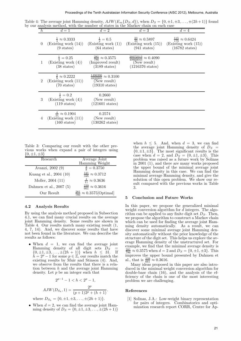
Table 4: The average joint Hamming density, AJW (Em{DS , d}), when DS = {0,±1,±3, . . . ,±(2h+1)} foundby our analysis method, with the number of states in the Markov chain on each case

h d = 1 d = 2 d = 3 d = 4

13 ≈ 0.3333 1

2 = 0.5 2339 ≈ 0.5897 115

179 ≈ 0.64240 (Existing work (14)) (Existing work (1)) (Existing work (15)) (Existing work (15))

(9 states) (64 states) (941 states) (16782 states)

14 = 0.25 281

786 ≈ 0.3575 2037251349809043 ≈ 0.4090

1 (Existing work (4)) (Improved result) (New result)(38 states) (3189 states) (1216376 states)

29 ≈ 0.2222 1496396

4826995 ≈ 0.31002 (Existing work (11)) (New result)

(70 states) (19310 states)

15 = 0.2 0.2660

3 (Existing work (4)) (New result)(119 states) (121601 states)

421 ≈ 0.1904 0.2574

4 (Existing work (11)) (New result)(160 states) (130262 states)

Table 3: Comparing our result with the other pre-vious works when expand a pair of integers using{0,±1,±3}

Research Average JointHamming Weight

Avanzi, 2002 (9) 38 = 0.3750

Kuang et al., 2004 (10) 121326 ≈ 0.3712

Moller, 2004 (11) 411 ≈ 0.3636

Dahmen et al., 2007 (5) 239661 ≈ 0.3616

Our Result 281786 ≈ 0.3575[Optimal]

4.2 Analysis Results

By using the analysis method proposed in Subsection4.1, we can find many crucial results on the averagejoint Hamming density. Some results are shown inTable 4. Our results match many existing result (1,4, 7, 14). And, we discover some results that havenot been found in the literature. We can describe theresults as follows:

• When d = 1, we can find the average jointHamming density of all digit sets DS ={0,±1,±3, . . . ,±(2h + 1)} when h ≤ 31. Ifh = 2p− 1 for some p ∈ Z, our results match theexisting results by Muir and Stinson (4). And,we observe from the results that there is a rela-tion between h and the average joint Hammingdensity. Let p be an integer such that

2p−1 − 1 < h < 2p − 1,

AJW (DSh, 1) =

2p

(p + 1)2p + (h + 1).

where DSh= {0,±1,±3, . . . ,±(2h + 1)}.

• When d = 2, we can find the average joint Ham-ming density of DS = {0,±1,±3, . . . ,±(2h+1)}

when h ≤ 5. And, when d = 3, we can findthe average joint Hamming density of DS ={0,±1,±3}. The most significant results is thecase when d = 2, and DS = {0,±1,±3}. Thisproblem was raised as a future work by Solinasin 2001 (1), and there are many works proposedthe upper bound of the minimal average jointHamming density in this case. We can find theminimal average Hamming density, and give thesolution of this open problem. We show our re-sult compared with the previous works in Table3.

5 Conclusion and Future Works

In this paper, we propose the generalized minimalweight conversion algorithm for d integers. The algo-rithm can be applied to any finite digit set DS . Then,we propose the algorithm to construct a Markov chainwhich can be used for finding the average joint Ham-ming density automatically. As a result, we candiscover some minimal average joint Hamming den-sity automatically without the prior knowledge of thestructure of the digit set. This helps us explore the av-erage Hamming density of the unstructured set. Forexample, we find that the minimal average density is281786 ≈ 0.3575 when d = 2 and DS = {0,±1,±3}. Thisimproves the upper bound presented by Dahmen etal., that is 239

661 ≈ 0.3616.Many ideas proposed in this paper are also intro-

duced in the minimal weight conversion algorithm fordouble-base chain (16), and the analysis of the ef-ficiency of the chain is one of the most interestingproblem we are challenging.

References

[1] Solinas, J.A.: Low-weight binary representationfor pairs of integers. Combinatorics and opti-mization research report CORR, Centre for Ap-


21

plied Cryptographic Research, University of Wa-terloo (2001)

[2] Heuberger, C., Muir, J.A.: Minimal weight andcolexicographically minimal integer representa-tion. Journal of Mathematical Cryptology 1(2007) 297–328

[3] Heuberger, C., Muir, J.A.: Unbalanced digitsets and the closest choice strategy for minimalweight integer representations. Designs, Codesand Cryptography 52(2) (2009) 185–208

[4] Muir, J.A., Stinson, D.R.: New minimal weightrepresentation for left-to-right window methods.Technical report, Department of Combinatoricsand Optimization, School of Computer Science,University of Waterloo (2004)

[5] Dahmen, E., Okeya, K., Takagi, T.: A new upperbound for the minimal density of joint represen-tations in elliptic curve cryptosystems. IEICETrans. Fundamentals E90-A(5) (2007) 952–959

[6] Dahmen, E., Okeya, K., Takagi, T.: An ad-vanced method for joint scalar multiplicationson memory constraint devices. In: Security andPrivacy in Ad-hoc and Sensor Networks. Vol-ume 3813/2005 of Lecture Notes in ComputerScience., Springer (2005) 189–204

[7] Dahmen, E.: Efficient algorithms for multi-scalar multiplications. Master’s thesis, Depart-ment of Mathematics, Technical University ofDarmstadt (2005)

[8] Okeya, K.: Joint sparse forms with twelveprecomputed points. IEICE Technical ReportIEICE-109(IEICE-ISEC-42) (2009) 43–50

[9] Avanzi, R.: On multi-exponentiation in cryp-tography. Cryptology ePrint Archive, 2002/154(2002)

[10] Kuang, B., Zhu, Y., Zhang, Y.: An improvedalgorithm for uP + vQ using JSF1

3. In: Ap-plied Cryptography and Network Security. Vol-ume 2004/3089 of Lecture Notes in ComputerScience., Springer (2004) 467–478

[11] Moller, B.: Fractional windows revis-ited:improved signed-digit representations for ef-ficient exponentiation. In: Information Securityand Cryptology - ICISC 2004. Volume 3506/2005of Lecture Notes in Computer Science., Springer(2005) 137–153

[12] Suppakitpaisarn, V., Edahiro, E., Imai, H.: Cal-culating Average Joint Hamming Weight forMinimal Weight Conversion of d Integers In:Workshop on Algorithms and Computation -WALCOM 2012. Lecture Notes in Computer Sci-ence., Springer (2012), (to be appeared)

[13] Haggstrom, O.: Finite Markov Chains and Algo-rithmic Application. 1 edn. Volume 52 of LondonMathematical Society, Student Texts. CambrideUniversity, Coventry, United Kingdom (2002)

[14] Egecioglu, O., Koc, C.K.: Exponentiation usingcanonical recoding. Theoretical Computer Sci-ence 129 (1994) 407–417

[15] Heuberger, C., Katti, R., Prodinger, H., Ruan,X.: The alternating greedy expansion and appli-cations to left-to-right algorithms. IEICE Trans.Fundamentals E90-A (2007) 341–356

[16] Suppakitpaisarn, V., Edahiro, E., Imai, H.: Fastelliptic curve cryptography using optimal double-base chains Cryptology ePrint Archive, Report2011/030 (2011)

[17] Schmidt, V.: Markov Chains and Monte-CarloSimulation. Department of Stochastics, Univer-sity Ulm (2006)

Appendix A: More Examples

In this section, we give more examples for better un-derstanding of the algorithm proposed in Section 3,4.Example 2 is the example for the minimal weight con-version in Section 3, and Examples 3,4 are the exam-ples for the Markov chain construction proposed inSection 4.

Example 2 Compute Em{{0,±1,±3}, 2}(23, 5) us-ing Algorithm 1,2.

• Eb{2}(23, 5) = 〈(10111), (00101)〉.

• When DS = {0,±1,±3}, Cs = {0,±1,±2,±3}.

• To simplify the explanation, we present it whenthe loop in Algorithm 1 Lines 4-7 assigned t to0, that is the last time on this loop. This meanswe have computed w1 and Q1. In this example,wt = 〈wt,Gt

〉Gtwhere Gt ∈ {0,±1,±2,±3}2. As

w1, Q1 has 49 elements, we are not able to listthem all. To show some elements of w1, Q1,

w1,〈0,0〉 = 3, w1,〈1,0〉 = 2, w1,〈2,0〉 = 3.

Q1,〈1,〈0,0〉〉 = (1011),

Q1,〈1,〈1,0〉〉 = (0300),

Q1,〈1,〈2,0〉〉 = (0301),

Q1,〈2,〈0,0〉〉 = (0010),

Q1,〈2,〈1,0〉〉 = (0010),

Q1,〈2,〈2,0〉〉 = (0010).

• Although, the loop in Algorithm 2 examines allG0 ∈ Cs2, we focus our interested the step whereG0 = 〈0〉. Note that in this case

AE ← 〈1, 1〉+ 〈0, 0〉 = 〈1, 1〉.

• Now, we focus our interested to the loop in Algo-rithm 2 Line 3-10. If R∗

0 = 〈0, 0〉, ae1 − r∗0,1 = 1and 2 - (ae1 − r∗0,1). Then, we〈0,0〉 ←∞.

• If R∗0 = 〈1, 1〉,

G1 ← 〈ae1 − r∗0,1

2,ae2 − r∗0,2

2〉 = 〈0, 0〉.

As stated on the first paragraph, w1,〈0,0〉 = 3.Then, we〈1,1〉 ← 3 + 0 = 3 by Line 6.

• If R∗0 = 〈−1,−3〉,

G1 ← 〈ae1 − r∗0,2

2,ae1 − r∗0,2

2〉 = 〈1, 2〉.

Then, we refer to w1,〈1,2〉 which is 1. Then,we〈−1,−3〉 ← 1 + 1 = 2.


22

• In Line 11, we select the least number among we,and the minimum value is we〈−1,−3〉 = 2. Then,w0,〈0,0〉 = 2.

Q0,〈1,〈0,0〉〉 ← 〈Q1,〈1,〈1,2〉〉,−1〉 = (03001̄).

Q0,〈2,〈0,0〉〉 ← 〈Q1,〈2,〈1,2〉〉,−3〉 = (01003̄),

which is the output of the algorithm.

Example 3 Construct the Markov chainA = (QA, Σ, σA, IA, PA) for findingAJW (Em{{0,±1}, 1}).

• As DS = {0,±1}, Cs = {0,±1}. Then,

w = 〈w〈−1〉, w〈0〉, w〈1〉〉.

The initial value of w, wI is

wI = 〈∞, 0,∞〉.

• Consider the loop in Lines 5-17. On the firstiteration, wx = wI in Line 7. If R is assigned to〈0〉 in Line 8, the result of the function MW inLine 9, wy is

wA = 〈1, 0, 1〉.

Then, we add α = 〈wI , 〈0〉, wA〉 to the set σA asshown in Line 10. The probability of the transi-tion α is 1

|Σ‖ = 1|{0,1}| = 1

2 . Also, we add wA to

the set Qu.

• Similarly, if R = 〈1〉, wy is

wB = 〈0, 1,∞〉.

Then, wB ∈ QA, and 〈wI , 〈1〉, wB〉 ∈ σA.

• Next, we explore the state wA, as we explore theset QA by the breadth-first search algorithm. IfR = 〈0〉, wy is 〈1, 0, 1〉. And if R = 〈1〉, wy is〈1, 1, 0〉. Then,

〈〈1, 0, 1〉, 〈0〉, 〈1, 0, 1〉〉 ∈ σA,

〈〈1, 0, 1〉, 〈1〉, 〈0, 1, 1〉〉 ∈ σA.

The first transition is the self-loop. Hence, weneed not to explore it again.

• We explore the state wB , the result is

〈〈0, 1,∞〉, 〈0〉, 〈1, 1, 2〉〉 ∈ σA,

〈〈0, 1,∞〉, 〈1〉, 〈1, 2,∞〉〉 ∈ σA.

We note that 〈1, 1, 2〉 is equivalent to 〈0, 0, 1〉,and we denote it as 〈0, 0, 1〉. Also, 〈1, 2,∞〉 isequivalent to 〈0, 1,∞〉. Then, the second transi-tion is the self-loop.

• Then, we explore the state 〈0, 1, 1〉. We get thecondition

〈〈0, 1, 1〉, 〈0〉, 〈1, 1, 2〉〉 ∈ σA,

〈〈0, 1, 1〉, 〈1〉, 〈1, 2, 1〉〉 ∈ σA.

We denote 〈1, 1, 2〉 and 〈1, 2, 1〉 by 〈0, 0, 1〉,〈0, 1, 0〉 respectively.

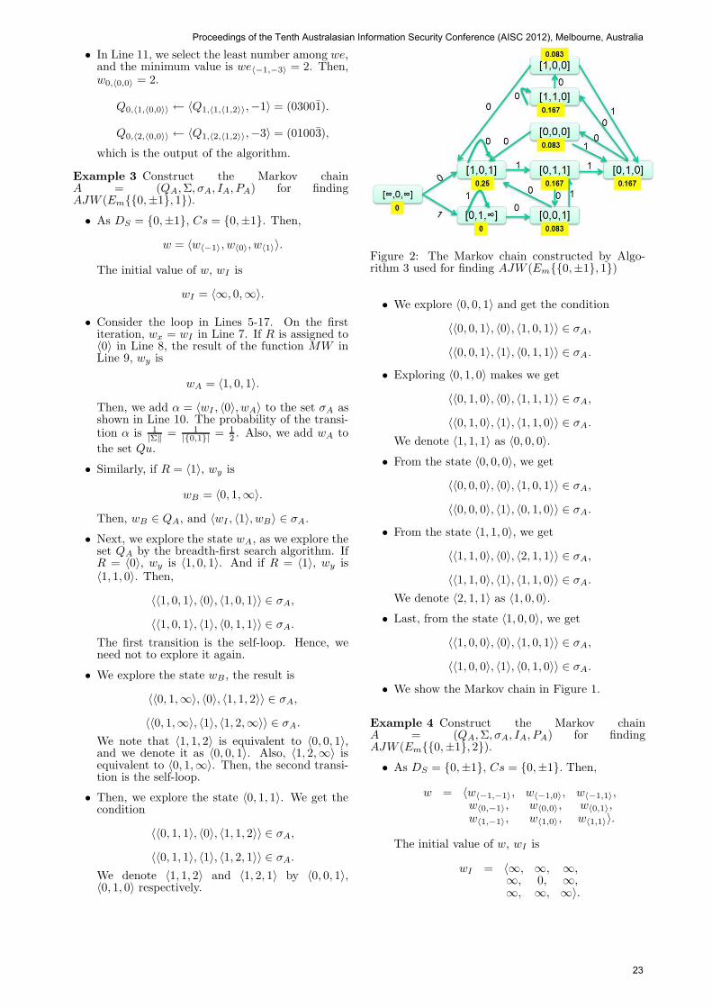
Figure 2: The Markov chain constructed by Algo-rithm 3 used for finding AJW (Em{{0,±1}, 1})

• We explore 〈0, 0, 1〉 and get the condition

〈〈0, 0, 1〉, 〈0〉, 〈1, 0, 1〉〉 ∈ σA,

〈〈0, 0, 1〉, 〈1〉, 〈0, 1, 1〉〉 ∈ σA.

• Exploring 〈0, 1, 0〉 makes we get

〈〈0, 1, 0〉, 〈0〉, 〈1, 1, 1〉〉 ∈ σA,

〈〈0, 1, 0〉, 〈1〉, 〈1, 1, 0〉〉 ∈ σA.

We denote 〈1, 1, 1〉 as 〈0, 0, 0〉.

• From the state 〈0, 0, 0〉, we get

〈〈0, 0, 0〉, 〈0〉, 〈1, 0, 1〉〉 ∈ σA,

〈〈0, 0, 0〉, 〈1〉, 〈0, 1, 0〉〉 ∈ σA.

• From the state 〈1, 1, 0〉, we get

〈〈1, 1, 0〉, 〈0〉, 〈2, 1, 1〉〉 ∈ σA,

〈〈1, 1, 0〉, 〈1〉, 〈1, 1, 0〉〉 ∈ σA.

We denote 〈2, 1, 1〉 as 〈1, 0, 0〉.

• Last, from the state 〈1, 0, 0〉, we get

〈〈1, 0, 0〉, 〈0〉, 〈1, 0, 1〉〉 ∈ σA,

〈〈1, 0, 0〉, 〈1〉, 〈0, 1, 0〉〉 ∈ σA.

• We show the Markov chain in Figure 1.

Example 4 Construct the Markov chainA = (QA, Σ, σA, IA, PA) for findingAJW (Em{{0,±1}, 2}).

• As DS = {0,±1}, Cs = {0,±1}. Then,

w = 〈w〈−1,−1〉, w〈−1,0〉, w〈−1,1〉,w〈0,−1〉, w〈0,0〉, w〈0,1〉,w〈1,−1〉, w〈1,0〉, w〈1,1〉〉.

The initial value of w, wI is

wI = 〈∞, ∞, ∞,∞, 0, ∞,∞, ∞, ∞〉.


23

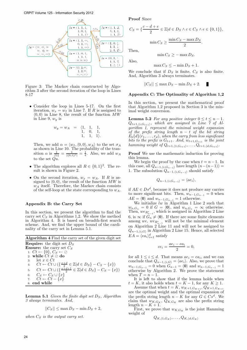
Figure 3: The Markov chain constructed by Algo-rithm 3 after the second iteration of the loop in Lines8-17

• Consider the loop in Lines 5-17. On the firstiteration, wx = wI in Line 7. If R is assigned to〈0, 0〉 in Line 8, the result of the function MWin Line 9, wy is

wy = wA = 〈1, 1, 1,1, 0, 1,1, 1, 1〉.

Then, we add α = 〈wI , 〈0, 0〉, wA〉 to the set σA

as shown in Line 10. The probability of the tran-sition α is 1

|Σ‖ = 1|{0,1}2| = 1

4 . Also, we add wA

to the set Qu.

• The algorithm explores all R ∈ {0, 1}2. The re-sult is shown in Figure 2.

• On the second iteration, wx = wA. If R is as-signed to 〈0, 0〉, the result of the function MW iswA itself. Therefore, the Markov chain consistsof the self-loop at the state corresponding to wA.

Appendix B: the Carry Set

In this section, we present the algorithm to find thecarry set CS in Algorithms 1,2. We show the methodin Algorithm 4. It is based on breadth-first searchscheme. And, we find the upper bound of the cardi-nality of the carry set in Lemma 5.1.

Algorithm 4 Find the carry set of the given digit set

Require: the digit set DS

Ensure: the carry set CS

1: Ct← {0}, CS ← �2: while Ct 6= � do3: let x ∈ Ct4: Ct← Ct ∪ ({x+d

2 ∈ Z|d ∈ DS} − CS − {x})

5: Ct← Ct ∪ ({x+d+12 ∈ Z|d ∈ DS} − CS − {x})

6: CS ← CS ∪ {x}7: Ct← Ct− {x}8: end while

Lemma 5.1 Given the finite digit set DS, Algorithm3 always terminates. And,

||CS || ≤ maxDS −min DS + 2,

when CS is the output carry set.

Proof Since

CS = {c− d + e

2∈ Z|d ∈ DS ∧ c ∈ CS ∧ e ∈ {0, 1}},

min CS ≥min CS −maxDS

2.

Then,min CS ≥ −maxDS .

Also,max CS ≤ −min DS + 1.

We conclude that if DS is finite, CS is also finite.And, Algorithm 3 always terminates.

||CS || ≤ maxDS −min DS + 2.

Appendix C: The Optimality of Algorithm 1,2

In this section, we present the mathematical proofthat Algorithm 1,2 proposed in Section 3 is the min-imal weight conversion.

Lemma 5.2 For any positive integer 0 ≤ t ≤ n− 1.Qt+1,〈i,Gt+1〉, which are assigned in Line 7 of Al-

gorithm 1, represent the minimal weight expansionof the prefix string length n − t of the bit stringEb{d}(r1, . . . , rd), when the carry from less significantbits to the prefix is Gt+1. And, wt+1,Gt+1

is the jointhamming weight of Qt+1,〈1,Gt+1〉, . . . , Qt+1,〈d,Gt+1〉.

Proof We use the mathematic induction for provingthis lemma.

We begin the proof by the case when t = n−1. Inthis case, all Qn−1,〈i,Gn−1〉 have length (n−(n−1)) =1. The subsolution Qn−1,〈i,Gn−1〉 should satisfy

Qn−1,〈i,Gn−1〉 = 〈aei〉,

if AE ∈ Dsd, because it does not produce any carriesto more significant bits. Then, wn−1,Gn−1

= 0 whenAE = 〈0〉 and wn−1,Gn−1

= 1 otherwise.We initialize lw in Algorithm 1 Line 2 such that

wn,Gn= 0 if G = 〈0〉, and wn,Gn

= ∞ otherwise.Then, weR∗

n−1, which is assigned in Algorithm 2 Line

6, is ∞ if Gn 6= 〈0〉. If there are some finite elementsamong we, weR∗

n−1will not be the minimal element

on Algorithm 2 Line 11 and will not be assigned toQn−1,〈i,G〉 in Algorithm 2 Line 15. Hence, all selected

EA = 〈eai〉di=1 satisfy

cei =aei − eai

2= 0,

for all 1 ≤ i ≤ d. That means aei = eai, and we canconclude that Qn−1,〈i,G〉 = 〈aei〉. Also, we prove thatwn−1,Gn−1

= 0 when Gn−1 = 〈0〉 and wn−1,Gn−1= 1

otherwise by Algorithm 2. We prove the statementwhen T = n− 1.

It is left to show that if the lemma holds whent = K, it also holds when t = K − 1, for any K ≥ 1.

Assume that when t = K, wK+1,GK+1, QK+1,GK+1

are the optimal weight and the optimal expansion ofthe prefix string length n−K for any G ∈ Csd. Weclaim that wK,GK

, QK,GKare also the prefix string

length n−K + 1.First, we prove that wK,GK

is the joint Hammingweight of

QK,〈1,GK〉, . . . , QK,〈d,GK〉


24

for any GK ∈ Csd. It is obvious that weEA selectedin Algorithm 2 Line 11 equals wK+1,CE , when EA =〈0〉 and wK+1,CE + 1 otherwise, by Algorithm 2 Line6 (CE is defined in Algorithm 2 Line 14). By theassignment in Algorithm 2 Line 15,

QK,〈i,GK〉 = 〈QK+1,〈i,CE〉, eai〉.

Since, the joint hamming weight ofQK+1,〈1,CE〉, . . . , QK+1,〈d,CE〉 is equal to wK+1,CE

by induction, the property also holds for each QK,GK.

Next, we prove the optimality of QK,〈i,GK〉.Assume contradiction that there are some stringPK,〈i,GK〉 such that

PK,〈i,GK〉 6= QK,〈i,GK〉

for some 1 ≤ i ≤ d, and some GK ∈ Csd. And, thejoint hamming weight of PK,〈1,GK〉, . . . , PK,〈d,GK〉 isless than QK,〈1,GK〉, . . . , QK,〈d,GK〉. Let the last digitof PK,〈i,GK〉 be lpi. If lpi = eai for all 1 ≤ i ≤ d, thecarry is

〈aei − eai

2〉di=1 = CE.

By induction, the joint Hamming weightQK+1,〈1,CE〉, . . . , QK+1,〈d,CE〉 is the minimal jointHamming weight. Then, the joint hamming weightof P is greater or equal to Q. If lpi 6= eai for some1 ≤ i ≤ d, the carry is

H = 〈hi〉di=1 = 〈

aei − lpi

2〉di=1.

By induction, QK+1,〈i,H〉 is the minimal weight ex-pansion. Then,

JW (PK,〈1,H〉, . . . , PK,〈d,H〉) ≥

W (QK+1,〈1,H〉, . . . , QK+1,〈d,H〉) + JW (〈lp1〉, . . . , 〈lpd〉),

when JW is the joint hamming weight function.By the definition of WE, it is clear that

JW (QK+1,〈1,H〉, . . . , QK+1,〈d,H〉) +

JW (〈lp1〉, . . . , 〈lpd〉) = weI ,

when I = 〈lp1, . . . , lpd〉.In Algorithm 2 Line 11, we select the minimal

value of weEA. That is

weEA ≤ weI .

As

weEA = JW (QK,〈1,GK〉, . . . , QK,〈d,GK〉),

we can conclude that

JW (PK,〈1,GK〉, . . . , PK,〈d,GK〉) ≥

JW (QK,〈1,G〉, . . . , QK,〈d,G〉).

This contradicts our assumption.

Theorem 5.3 Let Z = 〈0〉. 〈Q0,〈i,Z〉〉di=1 in Algo-

rithm 1 Line 9 is the minimal joint weight expansionof r1, . . . , rd on digit set Ds.

Proof 〈Q0,〈i,G〉〉di=1 are the optimal binary expansion

of the least significant bit by Lemma 5.2. Since thereis no carry to the least significant bit, 〈Q0,〈i,{0}〉〉

di=1

is the optimal solution.


25


26

Documents

Fast Elliptic Curve Cryptography Using Minimal …crpit.com/confpapers/CRPITV125Suppakitpaisarn.pdfFast Elliptic Curve Cryptography Using Minimal Weight Conversion of d Integers Vorapong