Embed Size (px)
Citation preview
Fast Nielsen–Thurston Classification
Oyku YurttasDicle University
joint w/ Dan Margalit, Balazs Strenner and Sam Taylor
Algorithms in Complex Dynamics and Mapping Class Groups
ICERMNovember 2, 2019
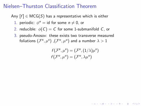
Nielsen–Thurston Classification Theorem
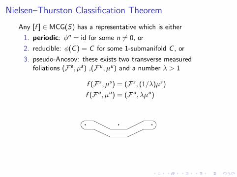
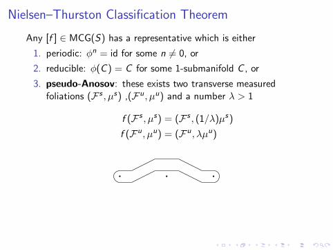
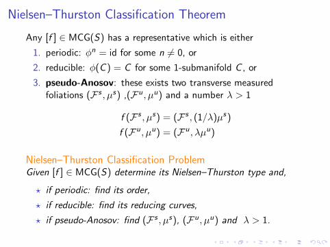
Any [f ] ∈ MCG(S) has a representative which is either
1. periodic: φn = id for some n 6= 0, or
2. reducible: φ(C ) = C for some 1-submanifold C , or
3. pseudo-Anosov: these exists two transverse measuredfoliations (F s , µs) ,(Fu , µu) and a number λ > 1
f (F s , µs) = (F s , (1/λ)µs )
f (Fu , µu) = (Fu , λµu)

Nielsen–Thurston Classification Theorem
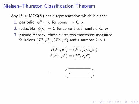
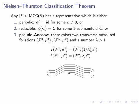
Any [f ] ∈ MCG(S) has a representative which is either
1. periodic: φn = id for some n 6= 0, or
2. reducible: φ(C ) = C for some 1-submanifold C , or
3. pseudo-Anosov: these exists two transverse measuredfoliations (F s , µs) ,(Fu , µu) and a number λ > 1
f (F s , µs) = (F s , (1/λ)µs )
f (Fu , µu) = (Fu , λµu)
Nielsen–Thurston Classification Theorem
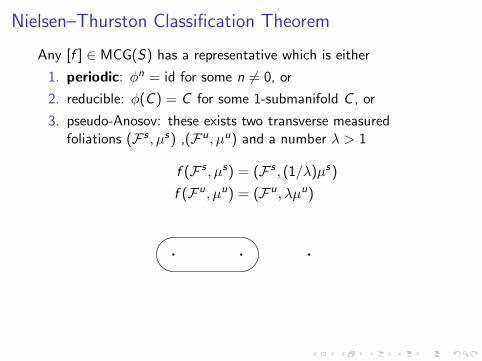
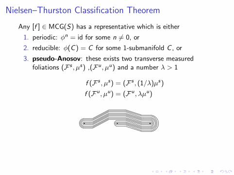
Any [f ] ∈ MCG(S) has a representative which is either
1. periodic: φn = id for some n 6= 0, or
2. reducible: φ(C ) = C for some 1-submanifold C , or
3. pseudo-Anosov: these exists two transverse measuredfoliations (F s , µs) ,(Fu , µu) and a number λ > 1
f (F s , µs) = (F s , (1/λ)µs )
f (Fu , µu) = (Fu , λµu)
Nielsen–Thurston Classification Theorem
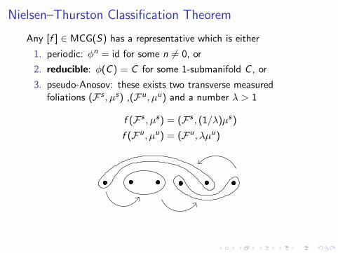
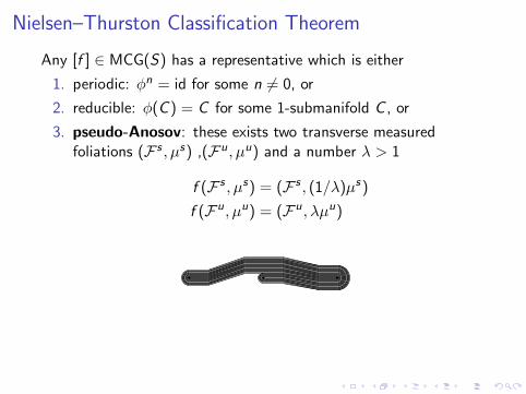
Any [f ] ∈ MCG(S) has a representative which is either
1. periodic: φn = id for some n 6= 0, or
2. reducible: φ(C ) = C for some 1-submanifold C , or
3. pseudo-Anosov: these exists two transverse measuredfoliations (F s , µs) ,(Fu , µu) and a number λ > 1
f (F s , µs) = (F s , (1/λ)µs )
f (Fu , µu) = (Fu , λµu)
Nielsen–Thurston Classification Theorem
Any [f ] ∈ MCG(S) has a representative which is either
1. periodic: φn = id for some n 6= 0, or
2. reducible: φ(C ) = C for some 1-submanifold C , or
3. pseudo-Anosov: these exists two transverse measuredfoliations (F s , µs) ,(Fu , µu) and a number λ > 1
f (F s , µs) = (F s , (1/λ)µs )
f (Fu , µu) = (Fu , λµu)
Nielsen–Thurston Classification ProblemGiven [f ] ∈ MCG(S) determine its Nielsen–Thurston type and,
⋆ if periodic: find its order,
⋆ if reducible: find its reducing curves,
⋆ if pseudo-Anosov: find (F s , µs), (Fu , µu) and λ > 1.
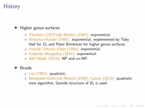
History
◮ Higher genus surfaces
⋆ Thurston (1970’s)& Mosher (1982): exponential.⋆ Bestvina–Handel (1995): exponential, implemented by Toby
Hall for Dn and Peter Brinkman for higher genus surfaces.⋆ Hamidi–Tehrani–Chen (1996): exponential.⋆ Koberda–Mangahas (2014): exponential.⋆ Bell–Webb (2016): NP and co–NP.
◮ Braids
⋆ Los (1993): quadratic.⋆ Bernadete-Gutierrez–Nitecki (1995), Calvez (2013): quadratic
time algorithm, Garside structure of Bn is used.

Main Theorem
Theorem in progress (Margalit–Taylor–Strenner–Y.)
There exists a quadratic time algorithm to solve theNielsen–Thurston classification problem.
Theorem (Bell–Webb)
Polynomial time algorithm to determine the Nielsen–Thurstonclassification type and find reducing curves, order and translationlength in the curve complex.

Basic Notions and TerminologyThroughout the talk we work on Dn.

Basic Notions and TerminologyThe results apply to any surface.
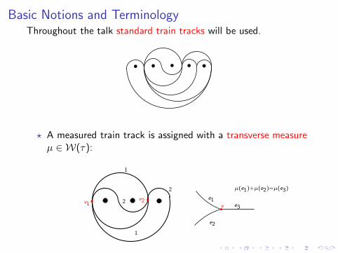
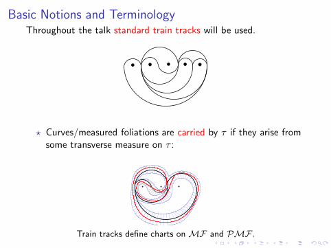
Basic Notions and TerminologyThroughout the talk standard train tracks will be used.
⋆ A measured train track is assigned with a transverse measureµ ∈ W(τ):
vv1
v2
1
1
2
2e1
e2
e3
µ(e1)+µ(e2)=µ(e3)

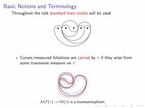
Basic Notions and TerminologyThroughout the talk standard train tracks will be used.
⋆ Curves/measured foliations are carried by τ if they arise fromsome transverse measure on τ :
1
1
2
2

Basic Notions and TerminologyThroughout the talk standard train tracks will be used.
⋆ Curves/measured foliations are carried by τ if they arise fromsome transverse measure on τ :

Basic Notions and TerminologyThroughout the talk standard train tracks will be used.
⋆ Curves/measured foliations are carried by τ if they arise fromsome transverse measure on τ :
C ≺ τ

Basic Notions and TerminologyThroughout the talk standard train tracks will be used.
⋆ Curves/measured foliations are carried by τ if they arise fromsome transverse measure on τ :
0.25
0.25
0.56
0.56

Basic Notions and TerminologyThroughout the talk standard train tracks will be used.
⋆ Curves/measured foliations are carried by τ if they arise fromsome transverse measure on τ :
collapse
collapse
collapse
(F , µ) ≺ τ

Basic Notions and TerminologyThroughout the talk standard train tracks will be used.
⋆ Curves/measured foliations are carried by τ if they arise fromsome transverse measure on τ :
C and F can smoothly be embedded inside N (τ):
Basic Notions and TerminologyThroughout the talk standard train tracks will be used.
⋆ Curves/measured foliations are carried by τ if they arise fromsome transverse measure on τ :
MF(τ) → W(τ) is a homeomorphism.
Basic Notions and TerminologyThroughout the talk standard train tracks will be used.
⋆ Curves/measured foliations are carried by τ if they arise fromsome transverse measure on τ :
Train tracks define charts on MF and PMF .

Basic Notions and TerminologyThroughout the talk standard train tracks will be used.
⋆ Train tracks define charts on MF and PMF .

Basic Notions and TerminologyThroughout the talk standard train tracks will be used.
⋆ Similar definition when a train track is carried by another traintrack:
τ
σ
σ ≺ τ
Basic Notions and TerminologyThroughout the talk standard train tracks will be used.
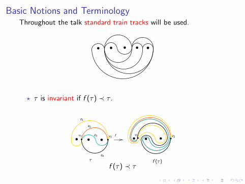
⋆ τ is invariant if f (τ) ≺ τ .
τ f (τ)
e1
e2
e3
e4
v1 v1v2 v2f
f (τ) ≺ τ

Basic Notions and TerminologyThroughout the talk standard train tracks will be used.
⋆ W(
f (τ))
⊆ W(τ).
τ f (τ)
e1
e2
e3
e4
v1 v1v2 v2f
f (τ) ≺ τ

Basic Notions and TerminologyThroughout the talk standard train tracks will be used.
⋆ By Brouwer Fixed Point Theorem f has a fixed point in W(τ).
τ f (τ)
e1
e2
e3
e4
v1 v1v2 v2f
f (τ) ≺ τ

Basic Notions and TerminologyThroughout the talk standard train tracks will be used.
⋆ One way to create σ carried by τ is to split τ :
��
��
����
��������
z z
z
t t
t
x x
xy
y y
x+y
x−y y−x

Basic Notions and TerminologyThroughout the talk standard train tracks will be used.
⋆ One way to create σ carried by τ is to split τ :
xxxx
xx
yy
y yy
y
x−y
x−y

Charts on PMF
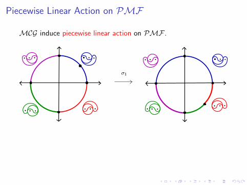
MCG induce piecewise linear action on PMF .

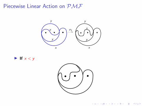
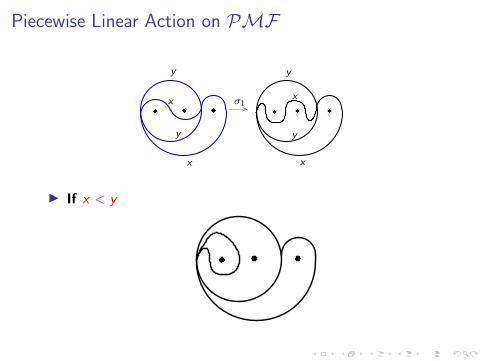
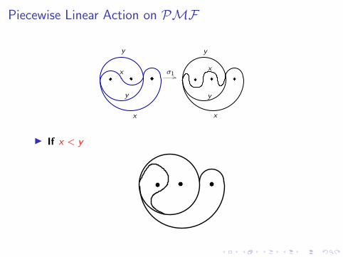
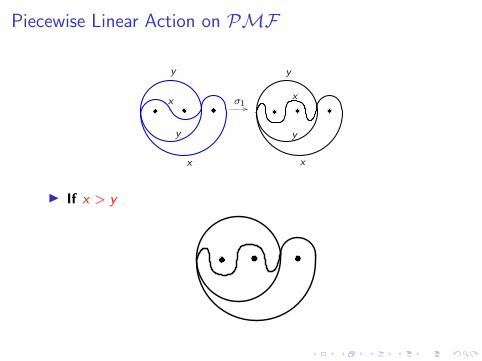
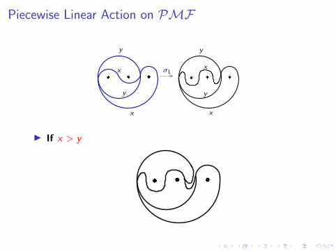
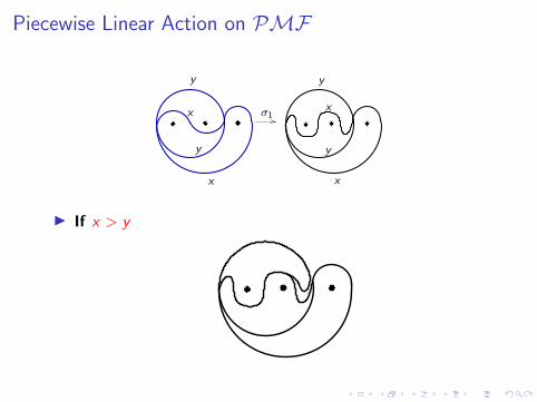
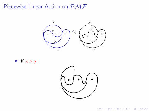
Piecewise Linear Action on PMF
��������
�� ������������
��������
��������
replacements
x
x
x
x
yy
yy
σ1

Piecewise Linear Action on PMF
��������
�� ������������
��������
��������
replacements
x
x
x
x
yy
yy
σ1
◮ If x < y
��������
����
��������
Piecewise Linear Action on PMF
��������
�� ������������
��������
��������
replacements
x
x
x
x
yy
yy
σ1
◮ If x < y
��������
����
��������
Piecewise Linear Action on PMF
��������
�� ������������
��������
��������
yy
yy
x
x
x
x σ1
◮ If x < y
��������
����
��������
Piecewise Linear Action on PMF
��������
�� ������������
��������
��������
yy
yy
x
x
x
x σ1
◮ If x < y
��������
����
��������

Piecewise Linear Action on PMF
��������
�� ������������
��������
��������
replacements
x
x
x
x
yy
yy
σ1
◮ If x < y the blue chart is mapped back to itself.
���� ����
��������
y−x
y−x
x
x
Piecewise Linear Action on PMF
��������
�� ������������
��������
��������
replacements
x
x
x
x
yy
yy
σ1
◮ If x > y
��������
����
��������
Piecewise Linear Action on PMF
��������
�� ������������
��������
��������
replacements
x
x
x
x
yy
yy
σ1
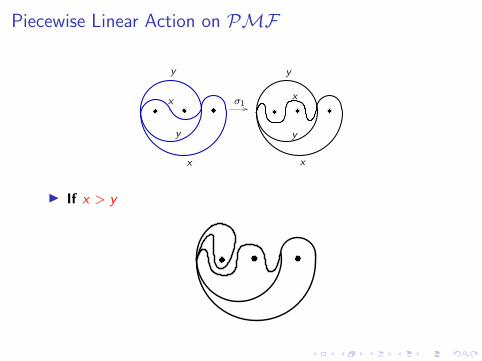
◮ If x > y
��������
����
��������
Piecewise Linear Action on PMF
��������
�� ������������
��������
��������
replacements
x
x
x
x
yy
yy
σ1
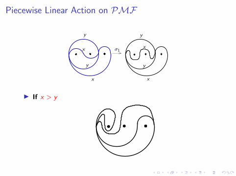
◮ If x > y
��������
����
��������
Piecewise Linear Action on PMF
��������
�� ������������
��������
��������
replacements
x
x
x
x
yy
yy
σ1
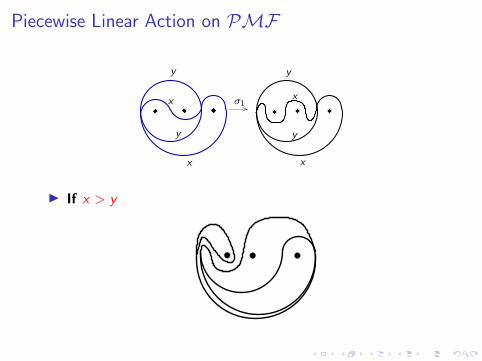
◮ If x > y
��������
����
��������
Piecewise Linear Action on PMF
��������
�� ������������
��������
��������
replacements
x
x
x
x
yy
yy
σ1
◮ If x > y
��������
����
��������
Piecewise Linear Action on PMF
��������
�� ������������
��������
��������
replacements
x
x
x
x
yy
yy
σ1
◮ If x > y
��������
�� ����

Piecewise Linear Action on PMF
��������
�� ������������
��������
��������
replacements
x
x
x
x
yy
yy
σ1
◮ If x > y
���� ���� ����
Piecewise Linear Action on PMF
��������
�� ������������
��������
��������
replacements
x
x
x
x
yy
yy
σ1
◮ If x > y

Piecewise Linear Action on PMF
��������
�� ������������
��������
��������
replacements
x
x
x
x
yy
yy
σ1
◮ If x > y

Piecewise Linear Action on PMF
��������
�� ������������
��������
��������
replacements
x
x
x
x
yy
yy
σ1
◮ If x > y the blue chart is mapped to the purple chart.
y
y
x−y
x−y
Piecewise Linear Action on PMF
MCG induce piecewise linear action on PMF .
σ1
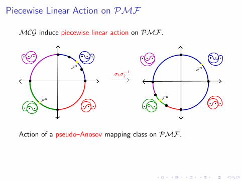
Piecewise Linear Action on PMF
MCG induce piecewise linear action on PMF .
FsF
s
Fu
Fu
σ1σ−12
Action of a pseudo–Anosov mapping class on PMF .
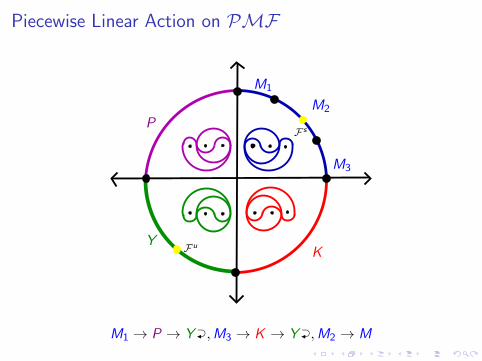
Piecewise Linear Action on PMF
����
����F s
Fu
M1
M2
M3
YK
P
M1 → P → Y ◭⊃,M3 → K → Y ◭
⊃,M2 → M
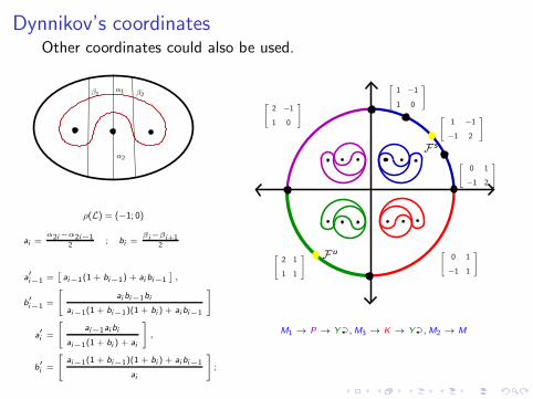
Dynnikov’s coordinatesOther coordinates could also be used.
α1
α2
β1 β2
ρ(L) = (−1; 0)
ai =α2i−α2i−1
2; bi =
βi−βi+12
a′
i−1 =[
ai−1(1 + bi−1) + ai bi−1]
,
b′
i−1 =
[
ai bi−1bi
ai−1(1 + bi−1)(1 + bi ) + ai bi−1
]
a′
i =
[
ai−1ai bi
ai−1(1 + bi ) + ai
]
,
b′
i =
[
ai−1(1 + bi−1)(1 + bi ) + ai bi−1
ai
]
;
����
��������
F s
Fu
[
1 −1
1 0
]
[
1 −1
−1 2
]
[
0 1
−1 2
]
[
2 −1
1 0
]
[
0 1
−1 1
]
[
2 1
1 1
]
M1 → P → Y ◭⊃,M3 → K → Y ◭⊃,M2 → M
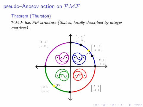
pseudo–Anosov action on PMF
Theorem (Thurston)
PMF has PIP structure (that is, locally described by integermatrices).
��������
����F
s
Fu
[
1 −1
1 0
]
[
1 −1
−1 2
]
[
0 1
−1 2
]
[
2 −1
1 0
]
[
0 1
−1 1
]
[
2 1
1 1
]
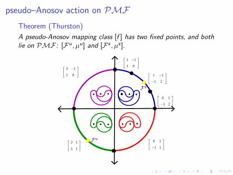
pseudo–Anosov action on PMF
Theorem (Thurston)
A pseudo-Anosov mapping class [f ] has two fixed points, and bothlie on PMF : [Fu , µu] and [F s , µs ].
��������
����F
s
Fu
[
1 −1
1 0
]
[
1 −1
−1 2
]
[
0 1
−1 2
]
[
2 −1
1 0
]
[
0 1
−1 1
]
[
2 1
1 1
]
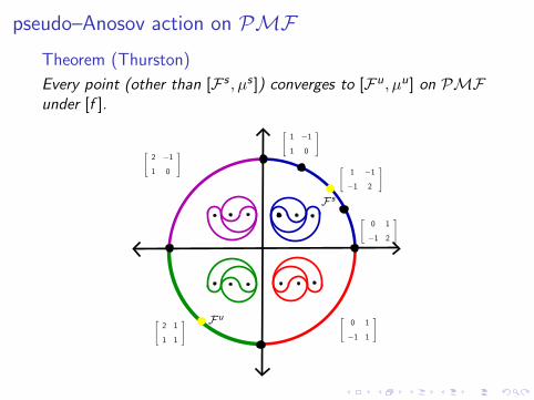
pseudo–Anosov action on PMF
Theorem (Thurston)
Every point (other than [F s , µs ]) converges to [Fu , µu] on PMFunder [f ].
��������
����F
s
Fu
[
1 −1
1 0
]
[
1 −1
−1 2
]
[
0 1
−1 2
]
[
2 −1
1 0
]
[
0 1
−1 1
]
[
2 1
1 1
]
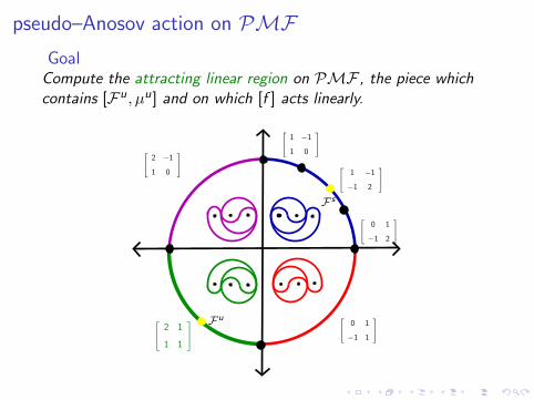
pseudo–Anosov action on PMF
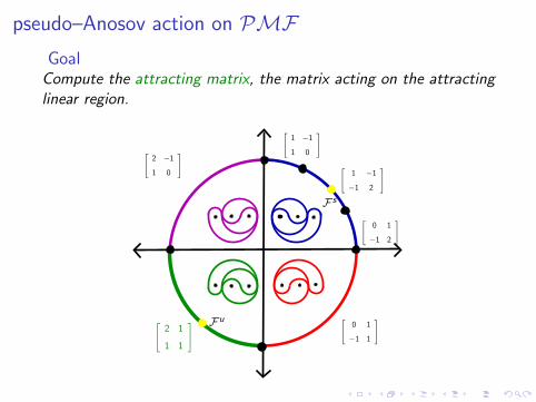
GoalCompute the attracting linear region on PMF , the piece whichcontains [Fu , µu] and on which [f ] acts linearly.
����
��������
Fs
Fu
[
1 −1
1 0
]
[
1 −1
−1 2
]
[
0 1
−1 2
]
[
2 −1
1 0
]
[
0 1
−1 1
]
[
2 1
1 1
]
pseudo–Anosov action on PMF
GoalCompute the attracting matrix, the matrix acting on the attractinglinear region.
����
��������
F s
Fu
[
1 −1
1 0
]
[
1 −1
−1 2
]
[
0 1
−1 2
]
[
2 −1
1 0
]
[
0 1
−1 1
]
[
2 1
1 1
]
pseudo–Anosov action on PMF
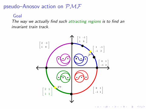
GoalThe way we actually find such attracting regions is to find aninvariant train track.
��������
����F
s
Fu
[
1 −1
1 0
]
[
1 −1
−1 2
]
[
0 1
−1 2
]
[
2 −1
1 0
]
[
0 1
−1 1
]
[
2 1
1 1
]
pseudo–Anosov action on PMF
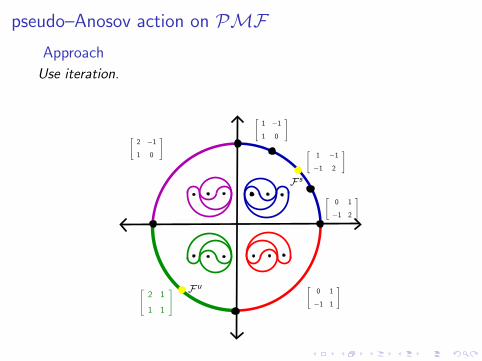
Approach
Use iteration.
��������
����F
s
Fu
[
1 −1
1 0
]
[
1 −1
−1 2
]
[
0 1
−1 2
]
[
2 −1
1 0
]
[
0 1
−1 1
]
[
2 1
1 1
]
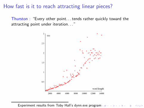
How fast is it to reach attracting linear pieces?
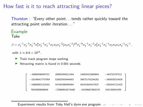
Thurston : “Every other point. . . tends rather quickly toward theattracting point under iteration. . . ”
Experiment results from Toby Hall’s dynn.exe program
How fast is it to reach attracting linear pieces?
Thurston : “Every other point. . . tends rather quickly toward theattracting point under iteration. . . ”
ExampleTake
β = σ−11 σ−3
2 σ−53 σ4
1σ−22 σ−1
3 σ1σ2σ−23 (σ2σ
−23 )19σ−8
1 σ−13 σ−2
1 σ22σ
−13 σ−1
1 σ2σ3σ1σ−12 σ−1
3 .
with λ ≈ 8.6× 10¹⁴.
◮ Train track program stops working.
◮ Attracting matrix is found in 0.001 seconds.
−68900596045753 200002959211464 146825523685804 −943752747512
−181490417757959 526825930446403 386751743244292 −2485930314639
−188609831321041 547491989409364 401923043417627 −2583447121425
76020009608848 −220669018174468 −161996823859176 1041269554295
Experiment results from Toby Hall’s dynn.exe program
How fast is it to reach invariant train tracks?
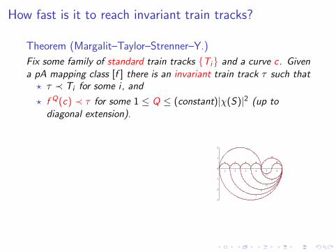
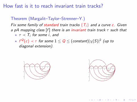
Theorem (Margalit–Taylor–Strenner–Y.)
Fix some family of standard train tracks {Ti} and a curve c. Givena pA mapping class [f ] there is an invariant train track τ such that
⋆ τ ≺ Ti for some i , and
⋆ f Q(c) ≺ τ for some 1 ≤ Q ≤ (constant)|χ(S)|2 (up todiagonal extension).
How fast is it to reach invariant train tracks?
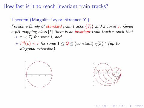
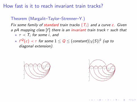
Theorem (Margalit–Taylor–Strenner–Y.)
Fix some family of standard train tracks {Ti} and a curve c. Givena pA mapping class [f ] there is an invariant train track τ such that
⋆ τ ≺ Ti for some i , and
⋆ f Q(c) ≺ τ for some 1 ≤ Q ≤ (constant)|χ(S)|2 (up todiagonal extension).
How fast is it to reach invariant train tracks?
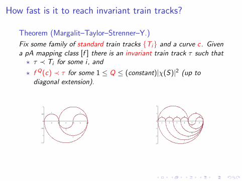
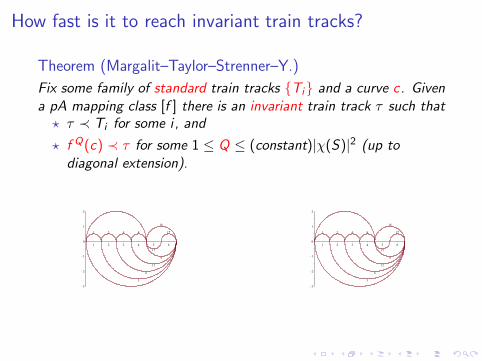
Theorem (Margalit–Taylor–Strenner–Y.)
Fix some family of standard train tracks {Ti} and a curve c. Givena pA mapping class [f ] there is an invariant train track τ such that
⋆ τ ≺ Ti for some i , and
⋆ f Q(c) ≺ τ for some 1 ≤ Q ≤ (constant)|χ(S)|2 (up todiagonal extension).

How fast is it to reach invariant train tracks?
Theorem (Margalit–Taylor–Strenner–Y.)
Fix some family of standard train tracks {Ti} and a curve c. Givena pA mapping class [f ] there is an invariant train track τ such that
⋆ τ ≺ Ti for some i , and
⋆ f Q(c) ≺ τ for some 1 ≤ Q ≤ (constant)|χ(S)|2 (up todiagonal extension).
How fast is it to reach invariant train tracks?
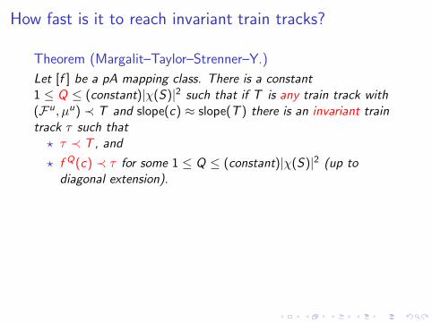
Theorem (Margalit–Taylor–Strenner–Y.)
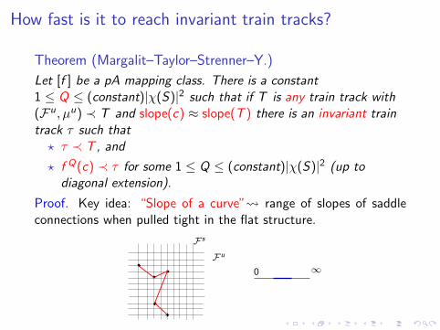
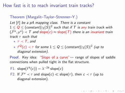
Let [f ] be a pA mapping class. There is a constant1 ≤ Q ≤ (constant)|χ(S)|2 such that if T is any train track with(Fu , µu) ≺ T and slope(c) ≈ slope(T ) there is an invariant traintrack τ such that
⋆ τ ≺ T, and
⋆ f Q(c) ≺ τ for some 1 ≤ Q ≤ (constant)|χ(S)|2 (up todiagonal extension).
How fast is it to reach invariant train tracks?
Theorem (Margalit–Taylor–Strenner–Y.)
Let [f ] be a pA mapping class. There is a constant1 ≤ Q ≤ (constant)|χ(S)|2 such that if T is any train track with(Fu , µu) ≺ T and slope(c) ≈ slope(T ) there is an invariant traintrack τ such that
⋆ τ ≺ T, and
⋆ f Q(c) ≺ τ for some 1 ≤ Q ≤ (constant)|χ(S)|2 (up todiagonal extension).
Proof. Key idea: “Slope of a curve” range of slopes of saddleconnections when pulled tight in the flat structure.
����
��
��
����
����
∞0
F s
Fu
How fast is it to reach invariant train tracks?
Theorem (Margalit–Taylor–Strenner–Y.)
Let [f ] be a pA mapping class. There is a constant1 ≤ Q ≤ (constant)|χ(S)|2 such that if T is any train track with(Fu , µu) ≺ T and slope(c) ≈ slope(T ) there is an invariant traintrack τ such that
⋆ τ ≺ T, and
⋆ f Q(c) ≺ τ for some 1 ≤ Q ≤ (constant)|χ(S)|2 (up todiagonal extension).
Proof. Key idea: “Slope of a curve” range of slopes of saddleconnections when pulled tight in the flat structure.
F1. slope(f k(c)) = λ−2k slope(c)
F2. If Fu ≺ τ and slope(c) ≪ slope(τ), then c ≺ τ (up todiagonal extension).
How fast is it to reach invariant train tracks?
����
��
��
����
��������
����
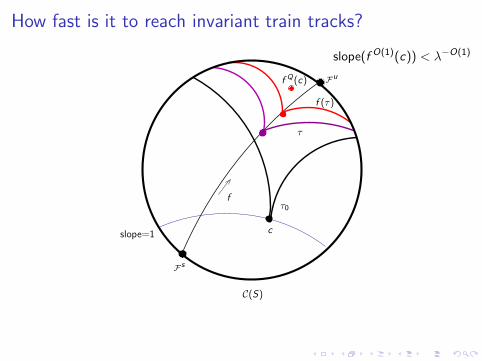
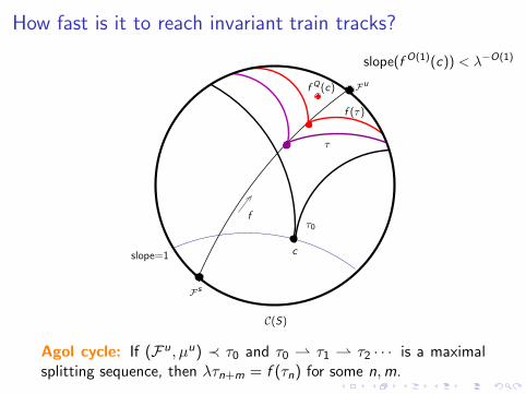
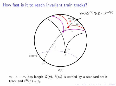
slope(f O(1)(c)) < λ−O(1)
τ0
τ
f (τ)
f
slope=1 c
Fs
Fu
C(S)
f Q(c)
How fast is it to reach invariant train tracks?
����
��
��
����
��������
����
slope(f O(1)(c)) < λ−O(1)
τ0
τ
f (τ)
f
slope=1 c
Fs
Fu
C(S)
f Q(c)
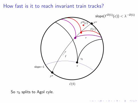
Agol cycle: If (Fu , µu) ≺ τ0 and τ0 ⇀ τ1 ⇀ τ2 · · · is a maximalsplitting sequence, then λτn+m = f (τn) for some n,m.
How fast is it to reach invariant train tracks?
����
��
��
����
��������
����
slope(f O(1)(c)) < λ−O(1)
τ0
τ
f (τ)
f
slope=1 c
Fs
Fu
C(S)
f Q(c)
So τ0 splits to Agol cyle.
How fast is it to reach invariant train tracks?
����
��
��
����
��������
����
slope(f O(1)(c)) < λ−O(1)
τ0
τ
f (τ)
f
slope=1 c
Fs
Fu
C(S)
f Q(c)
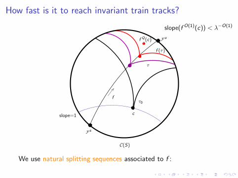
We use natural splitting sequences associated to f :
How fast is it to reach invariant train tracks?
����
��
��
����
��������
����
slope(f O(1)(c)) < λ−O(1)
τ0
τ
f (τ)
f
slope=1 c
Fs
Fu
C(S)
f Q(c)
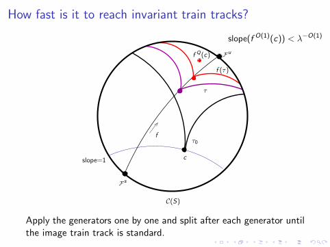
Apply the generators one by one and split after each generator untilthe image train track is standard.
How fast is it to reach invariant train tracks?
����
��
��
����
��������
����
slope(f O(1)(c)) < λ−O(1)
τ0
τ
f (τ)
f
slope=1 c
Fs
Fu
C(S)
f Q(c)
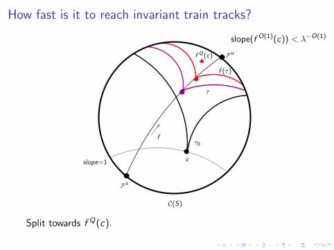
Split towards f Q(c).
How fast is it to reach invariant train tracks?
����
��
��
����
��������
����
slope(f O(1)(c)) < λ−O(1)
τ0
τ
f (τ)
f
slope=1 c
Fs
Fu
C(S)
f Q(c)
τ0 ⇀ · · · τn has length O(n), f (τn) is carried by a standard traintrack and f Q(c) ≺ τn.
How fast is it to reach invariant train tracks?
��������
����
��
��
��������
����
����
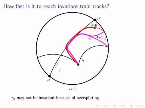
τ0
τn
f (τn)
fc
Fs
Fu
C(S)
f Q(c)
τn may not be invariant because of oversplitting.
How fast is it to reach invariant train tracks?
����
����
����
����
��������
����
����
����
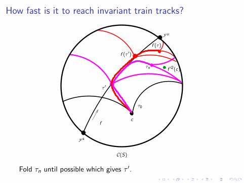
τ0
τ ′
f (τ ′)
τn
f (τ)
fc
Fs
Fu
C(S)
f Q(c)
Fold τn until possible which gives τ ′.
How fast is it to reach invariant train tracks?
����
����
����
����
����
��������
���
���
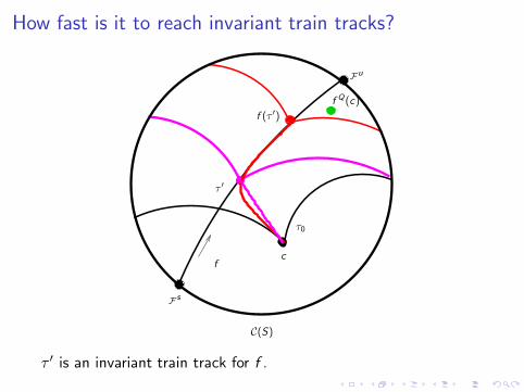
τ0
τ ′
f (τ ′)
fc
Fs
Fu
C(S)
f Q(c)
τ ′ is an invariant train track for f .
How fast is it to reach invariant train tracks?
����
����
����
����
����
��������
���
���
τ0
τ ′
f (τ ′)
fc
Fs
Fu
C(S)
f Q(c)
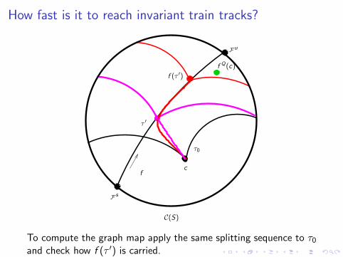
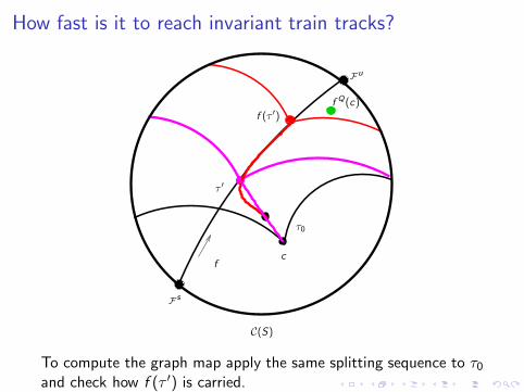
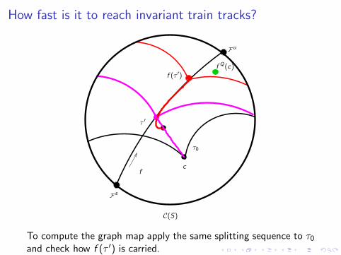
To compute the graph map apply the same splitting sequence to τ0and check how f (τ ′) is carried.
How fast is it to reach invariant train tracks?
����
��
����
����
����
��
���
���
τ0
τ ′
f (τ ′)
fc
Fs
Fu
C(S)
f Q(c)
To compute the graph map apply the same splitting sequence to τ0and check how f (τ ′) is carried.
How fast is it to reach invariant train tracks?
����
��
����
����
����
����
���
���
τ0
τ ′
f (τ ′)
fc
Fs
Fu
C(S)
f Q(c)
To compute the graph map apply the same splitting sequence to τ0and check how f (τ ′) is carried.

How fast is it to reach invariant train tracks?
����
��
����
����
����
��
���
���
τ0
τ ′
f (τ ′)
fc
Fs
Fu
C(S)
f Q(c)
To compute the graph map apply the same splitting sequence to τ0and check how f (τ ′) is carried.
How fast is it to reach invariant train tracks?
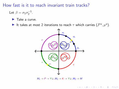
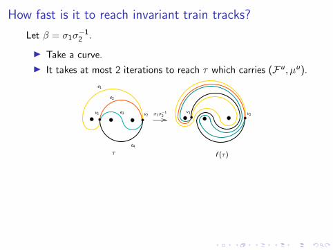
Let β = σ1σ−12 .
◮ Take a curve.
◮ It takes at most 2 iterations to reach τ which carries (Fu , µu).
��������
����F s
Fu
M1
M2
M3
YK
P
M1 → P → Y ◭⊃,M3 → K → Y ◭
⊃,M2 → M
How fast is it to reach invariant train tracks?
Let β = σ1σ−12 .
◮ Take a curve.
◮ It takes at most 2 iterations to reach τ which carries (Fu , µu).
τ f (τ)
e1
e2
e3
e4
v1 v1v2 v2σ1σ−12
How fast is it to reach invariant train tracks?
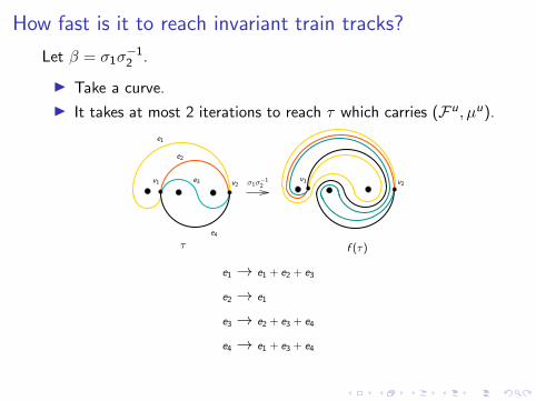
Let β = σ1σ−12 .
◮ Take a curve.
◮ It takes at most 2 iterations to reach τ which carries (Fu , µu).
τ f (τ)
e1
e2
e3
e4
v1 v1v2 v2σ1σ−12
e1 → e1 + e2 + e3
e2 → e1
e3 → e2 + e3 + e4
e4 → e1 + e3 + e4
How fast is it to reach invariant train tracks?
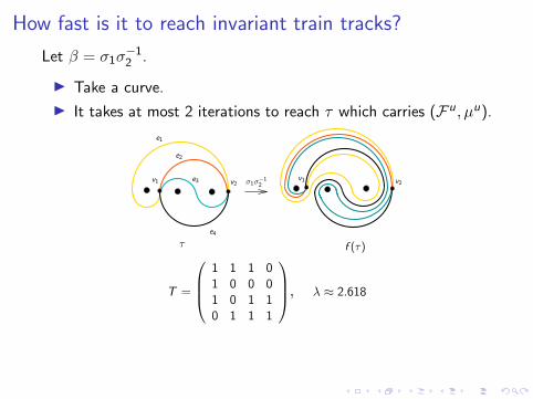
Let β = σ1σ−12 .
◮ Take a curve.
◮ It takes at most 2 iterations to reach τ which carries (Fu , µu).
τ f (τ)
e1
e2
e3
e4
v1 v1v2 v2σ1σ−12
T =
1 1 1 01 0 0 01 0 1 10 1 1 1
, λ ≈ 2.618
How fast is it to reach invariant train tracks?
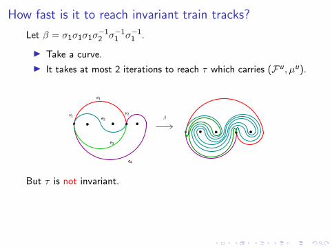
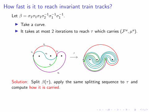
Let β = σ1σ1σ1σ−12 σ−1
1 σ−11 .
◮ Take a curve.
◮ It takes at most 2 iterations to reach τ which carries (Fu , µu).
e1
e2
e3
e4
v1v2
β
But τ is not invariant.
How fast is it to reach invariant train tracks?
Let β = σ1σ1σ1σ−12 σ−1
1 σ−11 .
◮ Take a curve.
◮ It takes at most 2 iterations to reach τ which carries (Fu , µu).
e1
e2
e3
e4
v1v2
β
Solution: Split β(τ), apply the same splitting sequence to τ andcompute how it is carried.
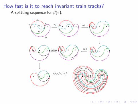
How fast is it to reach invariant train tracks?A splitting sequence for β(τ):
e1
σ1
split
split
isotopy
σ1σ1σ−12 σ−1
1 σ−11
e2
e3
e4
v1v2
How fast is it to reach invariant train tracks?
Same splitting sequence for τ :
e1 e1
e2 e2
e3e3
e4
e4
v1
v1v2
v2
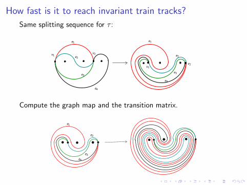
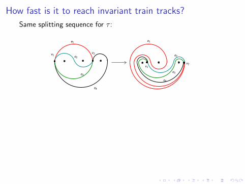
How fast is it to reach invariant train tracks?
Same splitting sequence for τ :
e1 e1
e2 e2
e3e3
e4
e4
v1
v1v2
v2
Compute the graph map and the transition matrix.
e1
e2
e3e4
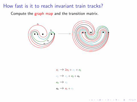
How fast is it to reach invariant train tracks?
Compute the graph map and the transition matrix.
e1
e2
e3e4
e1 → 2e1 + e2 + e3
e2 → e2 + e3 + e4
e3 → e2
e4 → e1 + e2
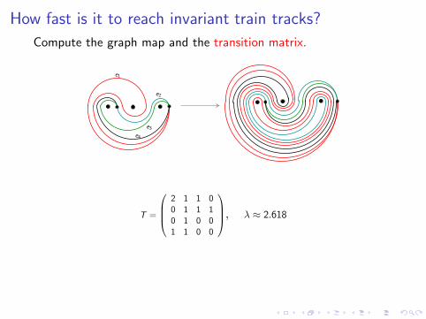
How fast is it to reach invariant train tracks?
Compute the graph map and the transition matrix.
e1
e2
e3e4
T =
2 1 1 00 1 1 10 1 0 01 1 0 0
, λ ≈ 2.618

How about reducibles?
Let β = σ1σ3σ1σ−12 σ4σ
−15 σ−1
3 σ−11 ∈ B6.
1
3
2
1
7
4
6
4
2

How about reducibles?
Let β = σ1σ3σ1σ−12 σ4σ
−15 σ−1
3 σ−11 ∈ B6.
1
3
2
1
7
4
6
4
2
f (τ) is not invariant.
����
�� ��������
����

How about reducibles?
Let β = σ1σ3σ1σ−12 σ4σ
−15 σ−1
3 σ−11 ∈ B6.
1
3
2
1
7
4
6
4
2
Reducing curves and partial pseudo-Anosovs appear after naturalsplitting sequence.
�� ��������
����
����

How about reducibles?
Let β = σ1σ3σ1σ−12 σ4σ
−15 σ−1
3 σ−11 ∈ B6.
1
3
2
1
7
4
6
4
2
Work under progress.
�� ��������
�� ����