情報工学実験4：データマイニング班tnal/2019/info3/dm/2019info4dm-w3.pdf · 情報工学実験4：データマイニング班 (week 3) 線形回帰モデルと最急降下法

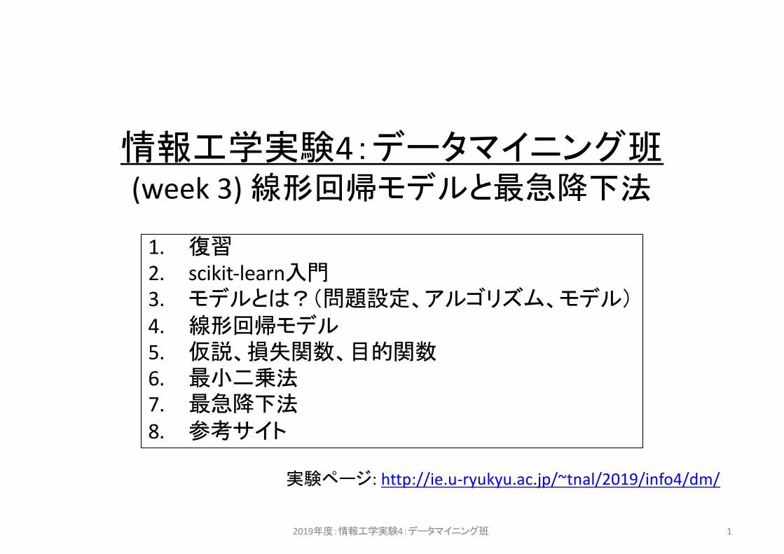
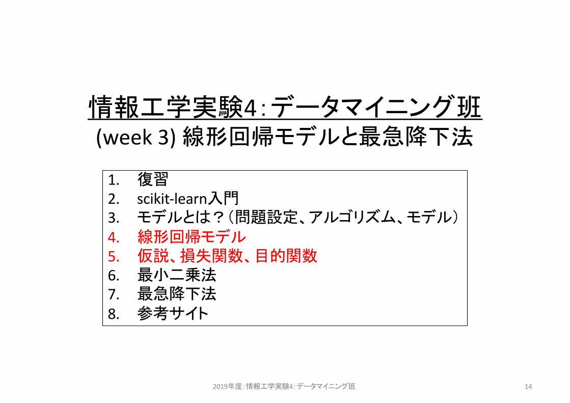
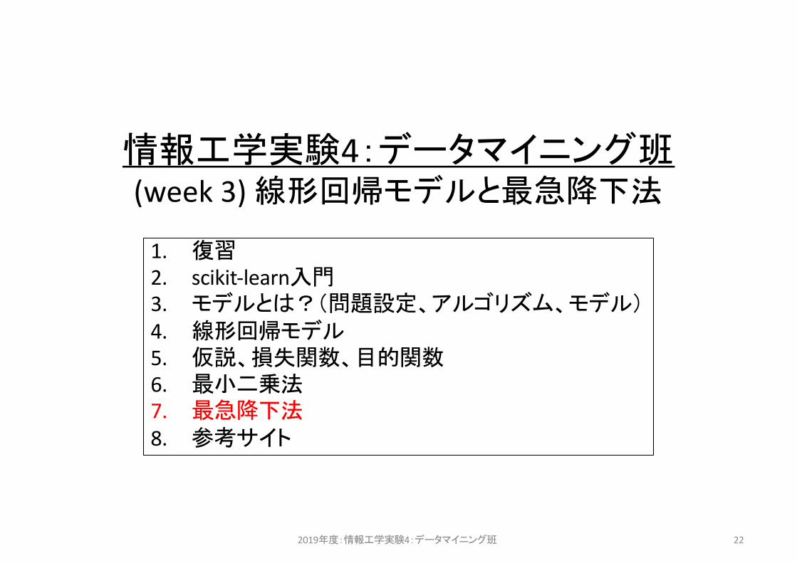
情報工学実験4：データマイニング班(week 3) 線形回帰モデルと最急降下法

1. 復習2. scikit-learn入門3. モデルとは？（問題設定、アルゴリズム、モデル）4. 線形回帰モデル5. 仮説、損失関数、目的関数6. 最小二乗法7. 最急降下法8. 参考サイト

2019年度：情報工学実験4：データマイニング班 1

実験ページ: http://ie.u-ryukyu.ac.jp/~tnal/2019/info4/dm/

http://ie.u-ryukyu.ac.jp/~tnal/2019/info4/dm/

Example: Iris flower data sethttp://en.wikipedia.org/wiki/Iris_flower_data_set

• Classification– In Classification, the samples belong to two or more

classes and we want to learn from already labeled data how to predict the class of unlabeled data.

– E.g., distinguishes the species from each other.– Dataset = samples vs. features and classes


1 sample

- Input data, X- 4 features or attributes

- Teach data- supervisory signal- output data, Y- target- 1 class in 3 classes

(1) What is experience E?(2) What is task T?

(3) How to measure the performance P?

review

http://en.wikipedia.org/wiki/Iris_flower_data_set

Example: boston house prices datasethttp://archive.ics.uci.edu/ml/datasets/Housing

• Regression– If the desired output consists of one or more continuous

variables, then the task is called regression.– E.g., concerns housing values in suburbs of Boston.– Dataset = samples vs. features and continuous variables


1 sample

13 features Continuous variable



CRIM ZN INDUS （中略） LSTAT MEDV

6.32E-03 1.80E+01 2.31E+00 4.98E+00 24.00

2.73E-02 0.00E+00 7.07E+00 9.14E+00 21.60

2.73E-02 0.00E+00 7.07E+00 4.03E+00 34.70

review

http://archive.ics.uci.edu/ml/datasets/Housing

Example: Overview of clustering methodshttps://scikit-learn.org/stable/modules/clustering.html

• Clustering– Clustering is the task of grouping a set of objects in such a way

that objects in the same group (called a cluster) are more similar (in some sense or another) to each other than to those in other groups (clusters).

– Training data consists of a set of input vectors x without any corresponding target values.

– Dataset = samples vs. features




review

https://scikit-learn.org/stable/modules/clustering.html

Terminology• ML types

– supervised, unsupervised, semi-supervised

– (reinforcement learning, genetic algorithm,,,)

• Task types– classification, regression,

clustering• sample• features, attributes

– numerical value– categorical value– true or false

• supervisory signal, teacher, class, label, target variable

• input, output• Input types

– training data / training set– test (for evaluation)– validation (for hyper

params)• model• parameters

– hyper parameters– weights, parameters

• learn, fit• predict, estimate• evaluation

– open or close test– cross validation


review




An introduction to machine learning with scikit-learn (1/3)

• Loading and an example dataset– python --version• Python 3.6.x or 3.7.x

– Example codesfrom sklearn import datasetsiris = datasets.load_iris() # datasets.load[tab]print(iris.DESCR)print(iris.data)print(iris.target)print(iris.target_names)


http://scikit-learn.org/stable/tutorial/basic/tutorial.html

https://github.com/naltoma/intro_jupyter_sklearn=> intro_sklearn.ipynb


https://github.com/naltoma/intro_jupyter_sklearn


• Learning and predictingfrom sklearn import svmclf = svm.SVC(gamma=0.001, C=100.)clf.fit(iris.data[:-1], iris.target[:-1])clf.predict(iris.data[-1:]]

# sklearn 0.17以降?, サンプル1個だと書き方に注意。

print(iris.target[-1])clf.score(iris.data, iris.target)





• Model persistence– # saveimport picklewith open('PredictiveModel.pickle', 'wb') as f:

pickle.dump(clf, f, pickle.HIGHEST_PROTOCOL)

– # loadwith open('PredictiveModel.pickle', 'rb') as f:

clf2 = pickle.load(f)

– # check the modelclf1.predict(iris.data) == clf2.predict(iris.data)







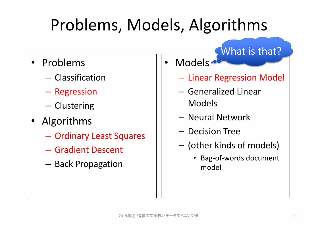
Problems, Models, Algorithms

• Problems– Classification– Regression– Clustering

• Algorithms– Ordinary Least Squares– Gradient Descent– Back Propagation

• Models– Linear Regression Model– Generalized Linear

Models– Neural Network– Decision Tree– (other kinds of models)

• Bag-of-words document model


What is that?

Models

• Represent by any formulas with (sometimes one) parameters for the relationship between input X’s and output Y’s.– In machine learning, the formulas called as

“hypothesis”.– E.g., h = a*x + b• a, b: parameters

– Parameterized model.– Predictive model. (e.g., a=1, b=2)


-5 -2.5 0 2.5 5

-2.5

2.5

Problem <-> Algorithm + Model


Data set

Learning Algorithm

hInput X’s Estimated value’s

hθ (x)=θ0x0 +θ1x1 = θi xi∑ = θiΦi (x)∑hθ (x)=θ0 +θ1x

Linear Regression Model

• How do we prepare a model?• How do we evaluate the goodness?• How do we choose the appropriate parameters?




Linear Regression Model• Training datasets– (x,y) = (4,7), (8,10), (13,11), (17,14)

• Hypothesis

• Parameters– θ0, θ1

• Cost function

• Objective function (measurement of the goodness)


J(θ0,θ1) =12m

(hθ (x(i) )− y(i) )2

i=1

m

∑

minθJ(θ0,θ1)

hθ (x) =θ0 +θ1xAssumption 1

Linear function

Assumption 2Squared error

Hypothesis vs. Cost function (θ1=1)

Hypothesis: Cost function:


h(x) = x

θ0=0, θ1=1, (x,y)=(4,7), (8,10), (13,11)

J(θ0,θ1) =12m

(hθ (x(i) )− y(i) )2

i=1

m

∑

0

5

10

15

20

0 5 10 15 20

y

x

"train.txt"x

J(0,1) = 12m((4− 7)2 + (8−10)2 + (13−11)2 )

J(0,1) = 12*3

(9+ 4+ 4) = 176= 2.83

0

5

10

15

20

-10 -5 0 5 10

Cos

t fun

ctio

n: J

(thet

a 1)

theta 1

"h1-sample1.dat"

0

5

10

15

20

0 5 10 15 20

y

x

"train.txt"0.5*x

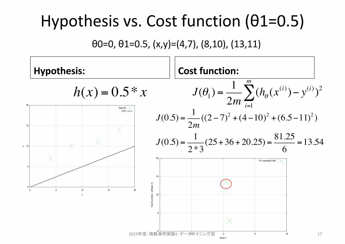
Hypothesis vs. Cost function (θ1=0.5)

Hypothesis: Cost function:


h(x) = 0.5* x

θ0=0, θ1=0.5, (x,y)=(4,7), (8,10), (13,11)

J(θ1) =12m

(hθ (x(i) )− y(i) )2

i=1

m

∑

0

5

10

15

20

-10 -5 0 5 10

Cos

t fun

ctio

n: J

(thet

a 1)

theta 1

"h1-sample2.dat"

J(0.5) = 12m((2− 7)2 + (4−10)2 + (6.5−11)2 )

J(0.5) = 12*3

(25+36+ 20.25) = 81.256

=13.54

Hypothesis vs. Cost function (θ1=others)

• θ1=0:– H(x)=0*x=0– J(0)=1/6{(0-4)^2+(0-10)^2+(0-13)^2}

• =1/6{16+100+169}=47.5• θ1=2:– H(x)=2*x– J(2)=1/6{(8-7)^2+(16-10)^2+(26-11)^2}

• =1/6{1+25+225}=41.83• θ1=1.5:– H(x)=1.5*x– J(1.5)=1/6{(6-7)^2+(12-10)^2+(19.5-11)^2}

• =1/6{1+4+72.25}=12.87


θ0=0, θ1=others, (x,y)=(4,7), (8,10), (13,11)

Objective function: minimize J(θ1)


0

5

10

15

20

-1 -0.5 0 0.5 1 1.5 2

Cos

t fun

ctio

n: J

(thet

a 1)

theta 1

"h1-sample5.dat"

Convex function

• How do we observe the shape of function?• How do we observe the behavior of GD?




Ordinary Least Squares


h(x) =θ0 +θ1x (x,y)=(4,7), (8,10), (13,11), (17,14)

θ0=1029/194≒5.28, θ1=48/97≒0.495h(x) = 5.28 + 0.495x

7 =θ0 + 4θ10 =θ0 + 4θ1 − 7e1 :=θ0 + 4θ1 − 7e12 = (θ0 + 4θ1 − 7)

2

E = ei2∑ ≥ 0

0

5

10

15

20

0 5 10 15 20

y

x

"train.txt"0.495*x+5.28

problems?

Ref., http://gihyo.jp/dev/serial/01/machine-learning/0008

= (θ0 + 4θ1 − 7)2 + (θ0 +8θ1 −10)

2 + (θ0 +13θ1 −11)2 + (θ0 +17θ1 −14)

2

= 538θ12 +84θ0θ1 + 4θ0

2 − 978θ1 −84θ0 + 466= (2θ1 + 21θ0 − 21)

2 + 97(θ0 − 48 / 97)2 +121/ 97

http://gihyo.jp/dev/serial/01/machine-learning/0008




Gradient descent algorithm


θi :=θi −α∂∂θi

J(θ0,θ1)Repeat until convergence {

}

(1) Start with any parameters.(2) Update the parameters simultaneously, until convergence.

Simple example

J(θ ) =θ 2,α = 0.1

• e.g., α=0. 1, θ=3, J(θ)=9• 1st update

• New_θ = 0.8*3 = 2.4• J(θ) = 2.4**2 = 5.76

• 2nd update• New_θ = 0.8*2.4 = 1.92• J(θ) = 1.92**2 = 3.6864

• 3rd update• New_θ = 1.536• J(θ) = 2.359296

• 4th update• New_θ = 1.2288000000000001• J(θ) = 1.5099494400000002

new_θ =θ −α ddθ

J(θ )

=θ − 0.1*2θ =θ − 0.2θ = 0.8θ

Cont.) the behavior of GD


0

5

10

15

20

25

-4 -2 0 2 4

J(th

eta

theta

"xx.dat"x*x

Gradient descent for Linear Regression


θi :=θi −α∂∂θi

J(θ0,θ1)

J(θ0,θ1) = 538θ12 +84θ0θ1 + 4θ0

2 − 978θ1 −84θ0 + 466• e.g., α=0.001, θ0=0, θ1=0, J(θ)=466• 1st update

• New_θ0 = 0 – 0.001*(-84) = 0.0084• New_θ1 = 0 – 0.001*(-978) = 0.0978• J(θ) = 374.86117384

• 2nd update• New_θ0 = 0.01597176• New_θ1 = 0.18500616• J(θ) = 302.3858537133122

• 3rd update• New_θ0 = 0.022804930848• New_θ1 = 0.2627653344• J(θ) = 244.75187010633334

• 4th update• New_θ0 = 0.0289794580943616• New_θ1 = 0.3321002229994368• J(θ) = 198.91981002677187

0

5

10

15

20

0 5 10 15 20

y

x

"train.txt"0

0.0084+0.0978*x0.01597176+0.18500616*x

0.022804930848+0.2627653344*x

∂∂θ0

J(θ0,θ1) = 84θ1 +8θ0 −84

∂∂θ1

J(θ0,θ1) =1076θ1 +84θ0 − 978

(x,y) = (4,7), (8,10), (13,11), (17,14)hθ (x) =θ0 +θ1x

(optional) zig-zagging behavior


Ref., http://en.wikipedia.org/wiki/Gradient_descent

http://en.wikipedia.org/wiki/Gradient_descent

References• Machine Learning | Coursera, https://class.coursera.org/ml-007• Gradient descent – Wikipedia,

http://en.wikipedia.org/wiki/Gradient_descent• 数理計画法第12回,

http://www.dais.is.tohoku.ac.jp/~shioura/teaching/mp11/mp11-12.pdf

• 機械学習はじめよう第8回線形回帰［前編］, http://gihyo.jp/dev/serial/01/machine-learning/0008

• 機械学習はじめよう第9回線形回帰［後編］, http://gihyo.jp/dev/serial/01/machine-learning/0009

• PRMLの線形回帰モデル（線形基底関数モデル）, http://www.slideshare.net/yasunoriozaki12/prml-29439402

• An introduction to machine learning with scikit-learn, http://scikit-learn.org/stable/tutorial/basic/tutorial.html


https://class.coursera.org/ml-007

http://en.wikipedia.org/wiki/Gradient_descent

http://www.dais.is.tohoku.ac.jp/~shioura/teaching/mp11/mp11-12.pdf



http://www.slideshare.net/yasunoriozaki12/prml-29439402


Documents

情報工学実験4：データマイニング班tnal/2019/info3/dm/2019info4dm-w3.pdf · 情報工学実験4：データマイニング班 (week 3) 線形回帰モデルと最急降下法