Feature extraction for image and point set analysis

Feature extraction for image and point set analysis

Demetrios P. Gerogiannis

P h . D . D i s s e r t a t i o n

– ♦ –

Ioannina, December 2014

ΤΜΗΜΑ ΜΗΧΑΝΙΚΩΝ Η/Υ & ΠΛΗΡΟΦΟΡΙΚΗΣ

ΠΑΝΕΠΙΣΤΗΜΙΟ ΙΩΑΝΝΙΝΩΝ

DEPARTMENT OF COMPUTER SCIENCE & ENGINEERING

UNIVERSITY OF IOANNINA

ÅîáãùãÞ ×áñáê�çñéó�éêþí ãéá

ÁíÜëõóç Åéêüíùí êáé Óçìåßùí

Ç ÄÉÄÁÊÔÏÑÉÊÇ ÄÉÁÔÑÉÂÇ

õðïâÜëëå�áé ó�çí

ïñéóèåßóá áðü �çí �åíéêÞ ÓõíÝëåõóç ÅéäéêÞò Óýíèåóçò

�ïõ ÔìÞìá�ïò Ìç÷áíéêþí Ç/Õ êáé �ëçñïöïñéêÞò

Åîå�áó�éêÞ Åðé�ñïðÞ

áðü �ïí

ÄçìÞ�ñéï �. �åñïãéÜííç

ùò ìÝñïò �ùí Õðï÷ñåþóåùí ãéá �ç ëÞøç �ïõ

ÄÉÄÁÊÔÏÑÉÊÏÕ ÄÉ�ËÙÌÁÔÏÓ ÓÔÇÍ �ËÇÑÏÖÏÑÉÊÇ

ÄåêÝìâñéïò 2014

"¼ðïéïò îÝñåé áðü ðñéí ðïý èÝëåé íá ðáÝé, äåí ðçãáßíåé ðïëý ìáêñéÜ."

ÍáðïëÝùí ÂïíáðÜñ�çò

Bolero, Mauri e Ravel

Committees

Advisory Committee:

Christophoros Nikou, Asso iate Professor, Department of Computer S ien e

and Engineering, University of Ioannina, Gree e (supervisor)

Aristidis Lykas, Professor, Department of Computer S ien e and Engineering,

University of Ioannina, Gree e

Ioannis Fudos, Asso iate Professor, Department of Computer S ien e and Engineering,


Examination Committee:

Christophoros Nikou, Asso iate Professor, Department of Computer S ien e

and Engineering, University of Ioannina, Gree e (supervisor)

Aristidis Lykas, Professor, Department of Computer S ien e and Engineering,


Ioannis Fudos, Asso iate Professor, Department of Computer S ien e and Engineering,


Antonios Argyros, Professor, Department of Computer S ien e,

University of Crete, Gree e

Ergina Kavallieratou, Assistant Professor, Department of Information and

Communi ation Systems Engineering, University of the Aegean, Gree e

Nikolaos Nikolaidis, Assistant Professor, Department of Computer S ien e,

Aristotle University of Thessaloniki, Gree e

Andreas Savakis, Professor, Department of Computer Engineering,

Ro hester Institute of Te hnology, Ro hester, NY, USA

Dedi ation

I wish to dedi ate this work to my parents. They inspired me to walk the path of

knowledge. An Itha a is rea hed, let us sail to a new one!

A knowledgements

I wish to thank my parents Panagiotis and Alexandra, my brother Thomas and my best

friends Kyriakos, George, Alexander for their material and moral support all those years

of study. Moreover, I wish to thank my supervisor, Prof. C. Nikou and Prof. A. Lykas for

their guidan e during my A ademi journey. We had a very onstru tive ollaboration.

Table of Contents

0.1 Overview . . . . . . . . . . . . . . . . . . . . . . . . . . . . . . . . . . . . .

0.2 Stru ture of the thesis . . . . . . . . . . . . . . . . . . . . . . . . . . . . .

I Features and Appli ations

1 Modeling sets of unordered points using line segments 1

1.1 Introdu tion . . . . . . . . . . . . . . . . . . . . . . . . . . . . . . . . . . . 1

1.2 A Dire t Split and Merge (DSaM) Framework for Line Segment Dete tion 3

1.2.1 Split Pro ess . . . . . . . . . . . . . . . . . . . . . . . . . . . . . . 3

1.2.2 Merge Pro ess . . . . . . . . . . . . . . . . . . . . . . . . . . . . . . 5

1.3 Evaluation of the Line Segment Dete tion Algorithm . . . . . . . . . . . . 6

1.3.1 Numeri al evaluation . . . . . . . . . . . . . . . . . . . . . . . . . . 7

1.3.2 Comparison with the Hough Transform . . . . . . . . . . . . . . . . 11

2 Appli ations 14

2.1 Vanishing Point Dete tion . . . . . . . . . . . . . . . . . . . . . . . . . . . 15

2.1.1 Introdu tion . . . . . . . . . . . . . . . . . . . . . . . . . . . . . . . 15

2.1.2 The algorithm . . . . . . . . . . . . . . . . . . . . . . . . . . . . . . 15

2.1.3 Numeri al Evaluation . . . . . . . . . . . . . . . . . . . . . . . . . . 17

2.2 Point loud sampling and re onstru tion . . . . . . . . . . . . . . . . . . . 21

2.2.1 Introdu tion . . . . . . . . . . . . . . . . . . . . . . . . . . . . . . . 21

2.2.2 The algorithm . . . . . . . . . . . . . . . . . . . . . . . . . . . . . . 22

2.2.3 Numeri al Evaluation . . . . . . . . . . . . . . . . . . . . . . . . . . 24

2.3 Shape en oding for edge map image ompression . . . . . . . . . . . . . . . 30

2.3.1 Introdu tion . . . . . . . . . . . . . . . . . . . . . . . . . . . . . . . 30

2.3.2 The algorithm . . . . . . . . . . . . . . . . . . . . . . . . . . . . . . 30


2.4 Retinal Fundus Image Feature Chara terization . . . . . . . . . . . . . . . 36

2.4.1 Introdu tion . . . . . . . . . . . . . . . . . . . . . . . . . . . . . . . 36

2.4.2 The algorithm . . . . . . . . . . . . . . . . . . . . . . . . . . . . . . 37


2.5 Elimination of outliers from 2D point sets using the Helmholtz prin iple . . 41

2.5.1 Introdu tion . . . . . . . . . . . . . . . . . . . . . . . . . . . . . . . 41

i

2.5.2 The Helmholtz prin iple . . . . . . . . . . . . . . . . . . . . . . . . 42

2.5.3 The algorithm . . . . . . . . . . . . . . . . . . . . . . . . . . . . . . 42


II Image and Point set Registration

3 Registering sets of points using Bayesian regression 42

3.1 Introdu tion . . . . . . . . . . . . . . . . . . . . . . . . . . . . . . . . . . . 42

3.2 Registration of sets of points via regression . . . . . . . . . . . . . . . . . . 45

3.3 Experimental Results and Dis ussion . . . . . . . . . . . . . . . . . . . . . 47

4 Registering images and sets of points using Mixture Models 59

4.1 Introdu tion . . . . . . . . . . . . . . . . . . . . . . . . . . . . . . . . . . . 59

4.2 Image registration with mixtures of Gaussian and Student's t-distributions 62

4.3 Robust registration of point sets with mixtures of Student's t-distributions 67

4.4 Experimental results . . . . . . . . . . . . . . . . . . . . . . . . . . . . . . 68

5 Epilogue 77

5.1 Con lusions . . . . . . . . . . . . . . . . . . . . . . . . . . . . . . . . . . . 77

5.2 Future Work . . . . . . . . . . . . . . . . . . . . . . . . . . . . . . . . . . . 79

I The Hungarian algorithm . . . . . . . . . . . . . . . . . . . . . . . . . . . 93

II Relevan e Ve tor Ma hines . . . . . . . . . . . . . . . . . . . . . . . . . . . 94

ii

List of Figures

1 Example of various images where line segments ould be used to des ribe

the depi ted information: (a) road ra ks, (b) maps, ( ) obje t edges, (d)

building edges, (e) road lanes. . . . . . . . . . . . . . . . . . . . . . . . . .

2 Example of images depi ting stru tured worlds. (a) Indoor s ene (b),( )

Outdoor s enes. . . . . . . . . . . . . . . . . . . . . . . . . . . . . . . . . .

3 Example of shape re onstru tion. (a) The initial set of points des ribing

a shape, (b) The hara teristi points (green stars) are extra ted from the

initial shape (red points), ( ) The re onstru tion result (blue points) super-

positioned over the initial shape (red points). Noti e the small deviation

between real and omputed data. . . . . . . . . . . . . . . . . . . . . . . .

4 Explanation of the registration problem. The goal is to determine that

geometri transformation that will be applied on the left image (yellow

ba kground) and will align the pixels su h that the pixels of the blue ir le

in the left will be mat hed with those of the green ir le in the right and

the pixels of the blue ellipse in the left will be orresponded with those of

the green ellipse in the right image. . . . . . . . . . . . . . . . . . . . . . .

1.1 Split pro ess. (a) At iteration t + 1, the ellipse with enter �

t

is split

into two new ellipses e1 and e2, with enters �

t+11 and �

t+12 given by (1.4).

(b) The new enters are marked with a star (*). The reassignment of the

points to the new enters is shown. Points of one ategory, assigned to e1,

are marked with a square, while points assigned to e2, are marked with a

ir le. . . . . . . . . . . . . . . . . . . . . . . . . . . . . . . . . . . . . . . 5

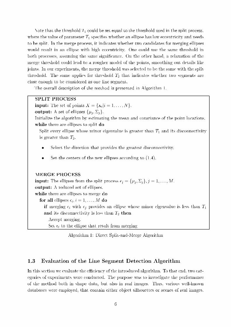
1.2 Steps of the split and merge pro ess. The pro ess is initialized with the

mean and the ovarian e of the full set of points. (a) Split into 2 ellipses.

(b) Split into 4 ellipses. ( ) End of split (35 ellipses). (d) The �nal merge

result (23 ellipses). The �gure is better seen in olor. . . . . . . . . . . . . 5

1.3 Some representative images of the databases we used in our experiments.

Please note that in some ases inner stru tures exist. This does not permit

to extra t an ordering of the points (a)MPEG7 [1℄, (b) Gatorbait [2℄, ( )

Brown [3℄, (d) ETHZ [4℄. . . . . . . . . . . . . . . . . . . . . . . . . . . . 8

iii

1.4 A representative result of the modeling of a shape from the MPEG7 dataset

[1℄with the proposed (left) and Kovesi [5℄ (right) methods. Green boxes

highlight the di�eren es regarding the modeling error of the two methods.

Although in general both methods modeled the shape globally, lo ally the

proposed method modeled more a urately the shape ontour. . . . . . . . 10

1.5 (a) - ( ) The primitive images used to reate the arti� ial dataset for ex-

periments with Gaussian additive noise. (d) Contour degraded by additive

Gaussian noise of 18dB. A representative test image produ ed by randomly

repeating the patterns of images in (a)-( ). . . . . . . . . . . . . . . . . . 11

1.6 Experimental results using the datasets of �gure 1.5 (e) that demonstrate

the performan e of our method in presen e of Gaussian additive noise in

terms of model omplexity error. The verti al axis represents the absolute

error between the real number of segments and the one omputed by our

method. . . . . . . . . . . . . . . . . . . . . . . . . . . . . . . . . . . . . . 12

1.7 (a)-( ) Results of the PPHT algorithm to a set of points representing the

shape of a bone (MPEG7 dataset) y varying the minimum number of points

in a bin (namely, 5, 15 and 25). Only a small fra tion of the lines is drawn

for visualization purposes. Note the overlapping lines. (d) The result of

our method. The �gure is better seen in olor. . . . . . . . . . . . . . . . 13

2.1 Πs

(x; a;b; �) for � = 50 and � = 1. . . . . . . . . . . . . . . . . . . . . . . 17

2.2 Representative results of the VP dete tion with the proposed method (the

�gure is better viewed in olor). . . . . . . . . . . . . . . . . . . . . . . . . 19

2.3 Representative results (the �gure is better viewed in olor). . . . . . . . . . 20

2.4 An example of the sampling pro ess. The bla k points represent the original

set of points, while the red line is the is their summary omputed by DSaM

[6℄. The verti al blue lines depi t the limits of the histogram bins. The

green points are those sele ted to represent the sampled set be ause they

are loser to the mean value of the bin. The �gure is better seen in olor. . 23

2.5 The value Æ = 1:6, whi h minimizes Φ(Æ) was used in our experiments. . . . 25

2.6 Representative results of sampling of the Gatorbait dataset [2℄. Details

of the upper left part of a �sh ontour. Sampling with (a) the proposed

method, (b) the method of Malik [7℄, ( ) Monte Carlo sampling and (d)

Random sampling. . . . . . . . . . . . . . . . . . . . . . . . . . . . . . . . 27

2.7 Shape re onstru tion of the Gatorbait dataset [2℄ using (a)-(b) DSaM, ( )-

(d)NN-S, (e)-(f) Kovesi [5℄, (g)-(h) vensor voting [8, 9℄. . . . . . . . . . . . 29

2.8 Representative results of the re onstru tion method on the Gatorbait [2℄

dataset. (a) The original image. Results extra ted with (b) DSaM [6℄, ( )

polygon approximation [10℄ with automati tuning (d) polygon approxima-

tion [10℄ with threshold value set to 5 pixels. . . . . . . . . . . . . . . . . . 34

iv

2.9 Representative results of the re onstru tion method on the MPEG7 [1℄

dataset. (a) The original image. Results extra ted with (b) DSaM [6℄, ( )

polygon approximation [10℄ with automati tuning (d) polygon approxima-

tion [10℄ with threshold value set to 5 pixels. . . . . . . . . . . . . . . . . . 34

2.10 Rate-distortion urves for (a) the Gatorbait dataset [2℄ and (b) the MPEG7

dataset [1℄. The blue line orresponds to the ompression results based on

DSaM [6℄ and the red line refers to polygon approximation [11℄. . . . . . . 35

2.11 An example of a video obje t plane. (a) The initial image, (b) the video

obje t plane mask and ( ) the re onstru tion result with the DSaM method.

The red points depi t the initial shape and and the green points show the

ontour re onstru ted with our method. . . . . . . . . . . . . . . . . . . . 35

2.12 The di�erent features that the proposed algorithm an dete t. The yellow

point is an end-point, the orange point is an interior-point and the green

point is a rossover. All the other points are jun tions (a T-jun tion is

shown in red, and a bifur ation is shown in blue). The image is better

viewed in olour. . . . . . . . . . . . . . . . . . . . . . . . . . . . . . . . . 36

2.13 An instan e of the point hara terization algorithm. Points x (in red and

bla k) orrespond to the thinned lines of the extra ted vessels. Green and

blue points are the extreme points y omputed by our DSaM algorithm.

The yellow ir le demonstrates the neighborhood of that point (N (y)).

Red and bla k points lying in that ir le are onsidered as neighbors of

that extreme point. In that ase, those points belong either to line luster

with index 1 or to line luster with index 2. Thus, CN (y) = 2. The

orange point orresponds to the nearest neighbor of y among the points of

neighbor line luster (bla k points). d is the minimum distan e between the

aforementioned nearest neighbor and the extreme points of its line luster. 38

2.14 (a) The original retinal image. (b) The manual segmentation of the vessels

in (a). ( ) Result of thinning the image in (b). (d) The on�den e regions

depi ted as ir les with a radius equal to 1% of the diagonal of the bounding

box of the original set. The �gure is better seen in olor. . . . . . . . . . . 39

2.15 The F measure, (2.10), for various values of parameter w in (2.9). The

bla k square indi ates the point that orresponds to the maximum value

of F measure. This value (F = 0:95) o urs for w = 2:9 and provides a

pre ision rate of 91:59% and a re all rate of 98:58%. More details are given

in se tion 2.4. . . . . . . . . . . . . . . . . . . . . . . . . . . . . . . . . . 40

2.16 (a) A a set of points (in red olor) degraded by equal in number outliers (in

blue olor). (b) The distribution of the sorted lengths of the line segments

approximating the point set of (a) using a line segment dete tion algorithm.

The horizontal axis represents the indi es of the segments and the verti al

axis represents the lengths. ( ) The Pareto distribution for various values

of the parameter a with b = 1. . . . . . . . . . . . . . . . . . . . . . . . . . 43

v

2.17 An example of the de�nition of the neighborhood of a segment. Points A

and B ( yan squares) are the starting/ending points of segment 1. The

yellow ir le with radius T determines the neighborhood. Line segments

2 and 3 are part of the neighborhood while segment 4 is not. The same

on�guration applies to point B. . . . . . . . . . . . . . . . . . . . . . . . . 44

2.18 Outlier elimination from the data set of Fig. 2.16(a) by (a) the �rst and

(b) the last iterations of the proposed method, ( ) Xian hao et al. [12℄, (d)

DBS an [13℄. The red boxes highlight representative false points provided

by the methods. . . . . . . . . . . . . . . . . . . . . . . . . . . . . . . . . 46

2.19 Boxplots of the line �tting errors for the ompared methods. Noti e the

di�erent s ales at the abs issas. . . . . . . . . . . . . . . . . . . . . . . . . 47

2.20 (a) A test image and (b) its degraded version at SNR = −1dB. . . . . . . . 48

2.21 Line segment modeling of image in �gure 2.20(b) omputed (a) by DSaM[6℄,

PA [10℄. Noti e that the PA is trapped by the outliers and produ es a large

number of short line segments, while DSaM manages to provide a valid model. 48

3.1 A false mat hing simulation example, with a point set used in [14℄. (a)

Corre t orresponden es between the sour e and the target sets are repre-

sented by line segments. (b) Two points were falsely mat hed on purpose

simulating a wrong orresponden e solution. The yellow box depi ts the

false mat hed points. ( ) The result of TPS [15℄. Noti e that large registra-

tion errors are present. (d) The result of the proposed registration s heme

based on RVM regression. In this ase the registration is orre t. . . . . . 45

3.2 The initial set of points used in our experiments, [14℄. (a) Sine, (b) Blob,

( ) Fish and (d) Ideogram. . . . . . . . . . . . . . . . . . . . . . . . . . . 50

3.3 (a) 2D range data used in our experiments [16℄. (b) 3D set of points

representing a fa e used in our experiments (3D fa e) [17℄. . . . . . . . . . 50

3.4 Rigid transformation experiment with 2D points of a range s an [16℄. (a)

Referen e set of points (red) and deformed set of points (bla k) of a 3D

fa e. (b) Registration result for the proposed method. . . . . . . . . . . . 50

3.5 Non rigid transformation experiment. (a) Referen e set of points (red)

and deformed set of points (bla k). Registration result for (b) CPD, ( )

RPM, (d) GMMReg and (e) the proposed method. The di�eren e is better

highlighted in olor. . . . . . . . . . . . . . . . . . . . . . . . . . . . . . . . 51

3.6 Non rigid transformation experiment. (a) Referen e set of points (red)

and deformed set of points (bla k). Registration result for (b) CPD, ( )

RPM, (d) GMMReg and (e) the proposed method. The di�eren e is better

highlighted in olor. . . . . . . . . . . . . . . . . . . . . . . . . . . . . . . 51

3.7 Non rigid transformation experiment with 3D points [17℄. (a) Referen e

set of points (red) and deformed set of points (bla k) of a 3D fa e. (b)

Registration result for the proposed method. . . . . . . . . . . . . . . . . 52

vi

3.8 Rigid transformation experiment in presen e of noise. (a) Referen e 2D

range set of points (red) and deformed set of points (bla k), [16℄ orrupted

with zero mean additive Gaussian noise. (b) Registration result for the

proposed method. The di�eren e is better highlighted in olor. . . . . . . 53

3.9 Non rigid transformation experiment in presen e of noise. (a) Referen e

set of points (red) and deformed set of points (bla k) orrupted with zero

mean additive Gaussian noise. Registration result for (b) CPD, ( ) RPM,

(d) GMMReg and (e) the proposed method. The di�eren e is better high-

lighted in olor. . . . . . . . . . . . . . . . . . . . . . . . . . . . . . . . . 53

3.10 Non rigid transformation experiment in presen e of noise. (a) Referen e

set of points (red) and deformed set of points (bla k) orrupted with zero

mean additive Gaussian noise. Registration result for (b) CPD, ( ) RPM,

(d) GMMReg and (e) the proposed method. The di�eren e is better high-

lighted in olor. . . . . . . . . . . . . . . . . . . . . . . . . . . . . . . . . 54

3.11 Non rigid transformation experiment in presen e of noise. (a) Referen e 3D

set of a fa e points (red) and deformed set of points (bla k), [17℄ orrupted

with zero mean additive Gaussian noise. (b) Registration result for the

proposed method. The di�eren e is better highlighted in olor. . . . . . . 54

3.12 Curves representing the number of points orre tly transformed with re-

spe t to a threshold determining the orre t transformation using RVM

(top row) and TPS (bottom row) when a number of initial false mat hes is

established in sour e and target sets. A point in the sour e set is orre tly

transformed if, after transformation, its distan e with respe t to its orre t

ounterpart is below the threshold. The left olumn shows results with

false assignments that preserve the one-to-one mat hing. In that ase the

RVM provides a onsistent behavior and its urves are all at 100% orre t

transformation. The right olumn shows results with false assignments that

do not preserve the one-to-one mat hing. . . . . . . . . . . . . . . . . . . . 57

3.13 Smoothness (3.4) of the RVM (top row) and TPS (bottom row) under var-

ious number of false mat hes. The left olumn shows results with false

assignments that preserve the one-to-one mat hing. Noti e that the s ale

of verti al axis at the top-left plot is 10−5indi ating a very smooth trans-

formation. The right olumn show results with false assignments that do

not preserve the one-to-one mat hing. . . . . . . . . . . . . . . . . . . . . . 58

4.1 A univariate Student's t-distribution (� = 0, � = 1) for various degrees of

freedom. As � → ∞ the distribution tends to a Gaussian. For small values

of � the distribution has heavier tails than a Gaussian. . . . . . . . . . . . 65

4.2 A 2D point set and the obtained models (a) GMM and (b) SMM. . . . . . 68

4.3 The point set of �gure 4.2 with 5% outliers and the obtained models by

(a) GMM and (b) SMM. Noti e that the GMM solution is a�e ted by the

outliers while the SMM is more robust. . . . . . . . . . . . . . . . . . . . 69

vii

4.4 (a) A three- lass pie ewise onstant image with intensity values 30, 125 and

220, and (b) its negative image ( orresponding values, 225, 130 and 35).

( ) The image in (a) degraded by uniform noise at 14 dB. This image was

then registered to the image in (b). The bottom line shows the registration

errors for the ompared methods. The ground truth solution is 0 deg for

the rotation and zero translation (the original image). (d) MI, (e) GMM,

(f) SMM. The errors present the di�eren e between the noise free registered

image and the referen e image. the values are s aled for better visualization. 70

4.5 Mean registration error versus signal to noise ratio (SNR) for the 3- lass

registration experiment of �gure 4.4. . . . . . . . . . . . . . . . . . . . . . 71

4.6 The obje tive fun tion in eq. (4.2) for the registration of the image of �gure

4.4(a) with its ounterpart rotated by 20 degrees and translated by 10 pixels. 71

4.7 A pair of NIH 3T3 ele tron mi ros ope images (400x magni� ation) of rat

ells under (a) normal and (b) uores ent light. . . . . . . . . . . . . . . . 72

4.8 (a) Image of Europe on 8 January 2007 at 01h00, provided by MeteoSat.

(b) Image of Europe on 9 January 2007 at 01h00, provided by MeteoSat

(by ourtesy of Meteo-Fran e). Noti e the large amount of outliers ( loudy

regions in di�erent lo ations in the image pair) introdu ing important dif-

� ulties in the registration pro ess. . . . . . . . . . . . . . . . . . . . . . . 73

4.9 Example of a set of points used in the experiments. (a) A point set (pre-

sented by dots) was generated by 3 Gaussians with means (−16; 9), (0; 5),

(18; 9) and spheri al ovarian e matri es of standard deviation 2. The

points were orrupted with 9% outliers. The resulting modeling of the noisy

set by (b) a 3- omponent GMM, ( ) a 4- omponent GMM with the fourth

omponent modeling the distribution of outliers and (d) a 3- omponent

SMM. . . . . . . . . . . . . . . . . . . . . . . . . . . . . . . . . . . . . . . 74

4.10 Registration error as a fun tion of outliers for the experiment presented in

�gure 4.9. . . . . . . . . . . . . . . . . . . . . . . . . . . . . . . . . . . . . 75

4.11 Modeling of a shaped point set from the GatorBait100 [2℄ data base by (a)

GMM with K = 30 omponents and (b) SMM with K = 30 omponents.

Noti e that the two models provided similar solutions. The bottom row

shows the modeling of the point set with 20% missing points and 10%

outliers by ( ) GMM and (d) SMM. Noti e that the solution of the SMM

was less a�e ted. In all ases the mixtures were similarly initialized using

the K-means algorithm. The axes in ( ) and (d) are normalized to the

range of the outliers. . . . . . . . . . . . . . . . . . . . . . . . . . . . . . . 76

viii

List of Tables

1.1 Short des ription of the databases used in our experiments. . . . . . . . . . 7

1.2 Modeling Error ∆ (1.1) . . . . . . . . . . . . . . . . . . . . . . . . . . . . . 8

1.3 Model Complexity MC (1.5) . . . . . . . . . . . . . . . . . . . . . . . . . . 9

2.1 Algorithm Performan e . . . . . . . . . . . . . . . . . . . . . . . . . . . . . 18

2.2 Number of two su essive frames where the distan e of the dete ted VP in

the two frames is less or equal to a threshold . . . . . . . . . . . . . . . . . 21

2.3 Hausdor� distan e between the original and the sampled sets using di�erent

sampling methods. . . . . . . . . . . . . . . . . . . . . . . . . . . . . . . . 26

2.4 Bull's Eye Rates for the retrieval of sampled sets using di�erent sampling

methods. . . . . . . . . . . . . . . . . . . . . . . . . . . . . . . . . . . . . . 27

2.5 Experimental results for the Gatorbait dataset [2℄ (38 shapes). . . . . . . . 33

2.6 Experimental results for the MPEG7 dataset [1℄ (1400 shapes). . . . . . . . 34

2.7 Experimental results for the VOP of �gure 2.11. . . . . . . . . . . . . . . . 36

2.8 Statisti s on the Hausdor� distan e (2.16) on the 38 shapes of the Gator-

Bait100 data set [2℄ . . . . . . . . . . . . . . . . . . . . . . . . . . . . . . . 46

2.9 Statisti s on the Hausdor� distan e (2.16) on the experiments based on the

test image of �gure 2.20(a). . . . . . . . . . . . . . . . . . . . . . . . . . . 48

3.1 Registration error statisti s for rigid transformations using di�erent kernels

on the shapes of �gure 3.2. The kernel width varies between 5% and 30%

of the mean varian e of the referen e set. . . . . . . . . . . . . . . . . . . . 48

3.2 Registration error statisti s for non rigid transformations using di�erent

kernels on the shapes of �gure 3.2. The kernel width varies between 5%

and 30% of the mean varian e of the referen e set. . . . . . . . . . . . . . . 48

3.3 Mean registration error for rigid transformations. . . . . . . . . . . . . . . 52

3.4 Mean registration error for non-rigid transformations. . . . . . . . . . . . . 52

3.5 Mean exe ution time (se ) of the ompared methods for the whole set of

experiments presented in se tion 3.3. The Hungarian-RVM is partially im-

plemented in Matlab (RVM training) and C (Hungarian algorithm). RPM

is totally implemented in Matlab while both CPD and GMMReg are totally

implemented in C. . . . . . . . . . . . . . . . . . . . . . . . . . . . . . . . 52

3.6 Average number of iterations of the ompared methods for the whole set

of experiments presented in se tion 3.3. . . . . . . . . . . . . . . . . . . . . 53

ix

3.7 Mean registration error for rigid transformations in presen e of noise. . . . 55

3.8 Mean registration error for non-rigid transformations in presen e of noise. . 55

3.9 Registration error statisti s for non-rigid transformations. . . . . . . . . . . 55

3.10 Registration error statisti s for non-rigid transformations. . . . . . . . . . . 56

4.1 Statisti s on the registration errors for the images in �g. 4.7 with varying

number of mixture omponents. The errors are expressed in pixels. . . . . . 72

4.2 Statisti s on the registration errors for the images in �g. 4.8 with varying

number of mixture omponents. The errors are expressed in pixels. . . . . . 73

4.3 Registration errors for the shaped point set of �gure 4.11 when it is or-

rupted by 15% outliers. . . . . . . . . . . . . . . . . . . . . . . . . . . . . . 76

x

Algorithm Index

1 Dire t Split-and-Merge Algorithm . . . . . . . . . . . . . . . . . . . . . . . 6

2 Vanishing point dete tion algorithm . . . . . . . . . . . . . . . . . . . . . . 18

3 Shape re onstru tion from a 2D point loud . . . . . . . . . . . . . . . . . 24

4 Image ompression . . . . . . . . . . . . . . . . . . . . . . . . . . . . . . . 31

5 Image de ompression . . . . . . . . . . . . . . . . . . . . . . . . . . . . . . 32

6 Rules for vessel features hara terization . . . . . . . . . . . . . . . . . . . 39

7 Outlier elimination based on the Helmholtz prin iple. . . . . . . . . . . . . 44

8 The RVM-Hungarian method for registration of sets of points . . . . . . . 47

9 The Hungarian algorithm for square ost matri es . . . . . . . . . . . . . . 94

10 The Hungarian algorithm for re tangular ost matri es (unbalan ed prob-

lems) . . . . . . . . . . . . . . . . . . . . . . . . . . . . . . . . . . . . . . . 95

Glossary

Brown A dataset used in experimental evaluation. It ontains 137 obje t silhouettes in

total, belonging to 13 di�erent ategories.

Dis onne tivity The dis onne tivity of two sets of points X, Y is the smallest distan e

between a point in X and a point in Y . It is used in the DSaM algorithm.

DSaM Dire t Split and Merge method for line segment dete tion.

EM Expe tation-Maximization algorithm. A framework that by optimizing the likeli-

hood extra ts the parameters of a model. In our work we used the EM algorithm

to train a GMM/SMM.

ETHZ A dataset used in experimental evaluation. It ontains 257 real images depi ting

s enes of 5 ategories (Gira�e, Cup, Swan, Apple Logo and Bottle).

Gatorbait100 A dataset used in experimental evaluation. It ontains 38 �sh silhouettes

in total, belonging to 8 di�erent ategories.

Linearity The linearity is a measure that des ribes how lose the points are to a straight

line. It is used in the DSaM algorithm.

MPEG7 A dataset used in experimental evaluation. It ontains 1400 obje t silhouettes

in total, belonging to 70 di�erent ategories.

VP The Vanishing Point is the point at whi h the parallel lines of a 3D real world image

are interse ted after proje ting them onto the 2D plane of an image.

Abstra t

Gerogiannis, Demetrios, P. PhD, Department of Computer S ien e and Engineering, Uni-

versity of Ioannina, Gree e. De ember, 2014. Feature Extra tion for Image and Point Set

Analysis. Thesis Supervisor: Christophoros Nikou.

This thesis is divided into two parts. The �rst part fo uses on an algorithm that �ts

line segments to a set of unordered points and its appli ation to omputer vision problems.

The method is based on the observation that a set of ollinear points are hara terized by

a ovarian e matrix whose minimum eigenvalue is low and therefore de�nes an e entri

(elongated) ellipse. At �rst, a single ellipse is �tted to the whole set of points whi h

is then iteratively split to a large number of highly e entri ellipses. Then, a merge

pro ess follows in order to ombine neighboring ellipses with almost ollinear major axes to

redu e the omplexity of the model. Experimental results on various databases show that

the proposed s heme is an eÆ ient te hnique for modeling unordered sets of points and

shapes by line segments. A number of omputer vision appli ation of the method are also

presented: the lo alization of the vanishing point in an image sequen e, the dete tion of

retinal fundus image features, su h as end-points, jun tions, and rossovers, an algorithm

for sampling image edges and a framework for modeling and removing outliers from a

set of unordered points. All of the above methods were su essfully ompared to various

alternative methods of the related literature and provided in general better results.

The se ond part of the thesis fo uses on the problem of image and point set registra-

tion. Registration is the pro ess of determining the parameters of a geometri transforma-

tion that brings into alignment two images or point sets. In this work, the images/point

sets to be registered are modeled by a mixture model and a method relying on the min-

imization of the distan e between distributions is proposed. We address the problems

of single and multimodal registration by employing both Gaussian mixture models and

mixtures of Student's -t distributions, whi h are robust to outliers. Moreover, we express

the task of registration as a Bayesian regression problem with by modeling the non rigid

transformation by relevan e ve tor ma hines whi h provide a losed form solution for the

estimation of the transformation. An iterative algorithm is presented whi h �rst deter-

mines the orresponden e between pixels/points in the two data images/points sets and

then the non rigid transformation is estimated based on that data asso iation.

Åê�å�áìÝíç �åñßëçøç ó�á ÅëëçíéêÜ

ÄçìÞ�ñéïò �åñïãéÜííçò �ïõ �áíáãéþ�ç êáé �çò ÁëåîÜíäñáò. PhD, ÔìÞìá Ìç÷áíéêþí Ç/Õ

êáé �ëçñïöïñéêÞò, �áíåðéó�Þìéï Éùáííßíùí, ÄåêÝìâñéïò, 2014. ÅîáãùãÞ ×áñáê�çñéó�éêþí

ãéá ÁíÜëõóç Åéêüíùí êáé Óçìåßùí. ÅðéâëÝðïí�áò: ×ñéó�üöïñïò Íßêïõ.

Ç ðáñïýóá äéá�ñéâÞ áðï�åëåß�áé áðü äýï èåìá�éêÝò åíü�ç�åò. Ó�çí ðñþ�ç åíü�ç�á

ðáñïõóéÜæå�áé ìßá ìÝèïäïò ìïí�åëïðïßçóçò åíüò óõíüëïõ ìç äéá�å�áãìÝíùí óçìåßùí áðü

Ýíá óýíïëï åõèõãñÜììùí �ìçìÜ�ùí êáé ç åöáñìïãÞ �çò óå äéÜöïñá ðñïâëÞìá�á õðïëïãéó�é-

êÞò üñáóçò. Ç ìÝèïäïò âáóßæå�áé ó�çí ðáñá�Þñçóç ü�é Ýíá óýíïëï óõíåõèåéáêþí óçìåßùí

÷áñáê�çñßæå�áé áðü Ýíáí ðßíáêá óõììå�áâëç�ü�ç�áò �ïõ ïðïßïõ ç åëÜ÷éó�ç éäéï�éìÞ Ý÷åé

ðïëý ìéêñÞ �éìÞ êáé ïñßæåé ìßá Ýëëåéøç ìå ìåãÜëç åêêåí�ñü�ç�á. Áñ÷éêÜ, �ï óýíïëï �ùí

óçìåßùí ðñïóåããßæå�áé áðü ìßá Ýëëåéøç ç ïðïßá ó�ç óõíÝ÷åéá äéá÷ùñßæå�áé åðáíáëçð�éêÜ

óå ðåñéóóü�åñåò åëëåßøåéò þó�å �ï óýíïëï �ùí óçìåßùí íá ðñïóåããéó�åß áðü Ýíáí áñéèìü

Ýêêåí�ñùí åëëåßøåùí. Ó�ç óõíÝ÷åéá, ëáìâÜíåé ÷þñá ìßá äéáäéêáóßá óõã÷þíåõóçò �ùí

åëëåßøåùí ðïõ Ý÷ïõí óõããñáìéêïýò ìÝãéó�ïõò Üîïíåò ãéá íá ìåéùèåß ç ðïëõðëïêü�ç�á �ïõ

ìïí�Ýëïõ. �åéñáìá�éêÜ áðï�åëÝóìá�á äåß÷íïõí �çí áðï�åëåóìá�éêü�ç�á �çò ìåèüäïõ íá

óõìðéÝæåé �çí ðëçñïöïñßá ìç äïìçìÝíùí óõíüëùí óçìåßùí áëëÜ êáé ó÷çìÜ�ùí. Åðßóçò,

ðáñïõóéÜæå�áé ç åöáñìïãÞ �çò ìåèüäïõ ó�ïí åí�ïðéóìü �ïõ óçìåßïõ äéáöõãÞò óå åéêïíïóåé-

ñÝò, ó�ïí åí�ïðéóìü êáé ÷áñáê�çñéóìü åéêüíùí �ïõ âõèïý �ïõ áìöéâëçó�ñïåéäïýò ÷é�þíá

�ïõ ïöèáëìïý, ó�ç äåéãìá�ïëçøßá ÷áñ�þí áêìþí áðü 2Ä åéêüíåò êáèþò êáé ó�çí åîÜëåéøç

�ïõ èïñýâïõ êáé áêñáßùí ìå�ñÞóåùí óå 2Ä óýíïëá óçìåßùí. ¼ëåò áõ�Ýò ïé ìÝèïäïé

óõãêñßíïí�áé åðé�õ÷þò ìå ìåèüäïõò �çò âéâëéïãñáößáò.

Ôï äåý�åñï ìÝñïò �çò äéá�ñéâÞò åó�éÜæåé ó�ï ðñüâëçìá �çò õðÝñèåóçò åéêüíùí êáé óõ-

íüëùí óçìåßùí. ÕðÝñèåóç åßíáé ç äéáäéêáóßá �çò åê�ßìçóçò �ïõ ãåùìå�ñéêïý ìå�áó÷çìá�é-

óìïý ðïõ öÝñíåé óå áí�éó�ïé÷ßá äýï óýíïëá óçìåßùí Þ åéêüíåò. Ó�çí åñãáóßá áõ�Þ, ïé

åéêüíåò/óýíïëá óçìåßùí ìïí�åëïðïéïýí�áé áðü ìéê�Ýò êá�áíïìÝò êáé ç õðÝñèåóç åðé�õã÷Üíå-

�áé ìå �çí åëá÷éó�ïðïßçóç �çò áðüó�áóçò ìå�áîý �ùí êá�áíïìþí. �ñï�åßíå�áé ç ìïí�åëïðïß-

çóç �ùí äåäïìÝíùí ìå ìéê�Ýò êáíïíéêÝò êá�áíïìÝò üóï êáé áðü ìéê�Ýò êá�áíïìÝò Student's

t ïé ïðïßåò åßíáé åýñùó�åò óå äåäïìÝíá ðïõ äåí áêïëïõèïýí �ï êõñßáñ÷ï ìïí�Ýëï.

Åðßóçò, ç äéáäéêáóßá �çò õðÝñèåóçò ðåñéãñÜöå�áé ùò Ýíá ðñüâëçìá ÌðåûæéáíÞò ðáëéíäñü-

ìçóçò ìå �ç ìïí�åëïðïßçóç �ïõ ìå�áó÷çìá�éóìïý áðü ìç÷áíÝò äéáíõóìÜ�ùí óõíÜöåéáò

(RVM) �á ïðïßá ðáñÝ÷ïõí ìßá êëåéó�Þò ìïñöÞò ëýóç ãéá �ï ãåùìå�ñéêü ìå�áó÷çìá�éóìü.

Ó�ï ðëáßóéï áõ�ü ðáñïõóéÜæå�áé Ýíáò åðáíáëçð�éêüò áëãüñéèìïò ðïõ åê�åëåß Ýíá âÞìá

áí�éó�ïß÷éóçò ìå�áîý �ùí åéêïíïó�ïé÷åßùí/óçìåßùí êáé ó�ç óõíÝ÷åéá ìå âÜóç áõ�Þ �çí

áí�éó�ïß÷éóç åê�éìÜåé �ïí åëáó�éêü ãåùìå�ñéêü ìå�áó÷çìá�éóìü ðïõ óõíäÝåé �á äýï óýíïëá.

Prologue

0.1 Overview

0.2 Stru ture of the thesis

0.1 Overview

The �eld of omputer vision has been advan ing during the last years, bene�ted from the

development of the te hnology and the available omputational resour es. Many methods

have been proposed in a high level to deal with the diÆ ult problem of simulating human

per eption. A ommon hara teristi of all these methods is that they are based on

preliminary feature extra tion te hniques to derive meaningful information from images

for further postpro essing.

Features are very basi entities that arry information related to a spe i� problem.

Computing features is performed via various algorithms and the pro ess is alled feature

extra tion and their representation may vary. A prin ipal hara teristi is that feature

models tend to be as simple as possible. Lines and line segments are widely used in the

omputer vision literature as feature representation models. They present low omplexity

and their aggregation an produ e more omplex models enabling the a urate represen-

tation of more omplex stru tures in an image. Sin e the early stages of the development

of the omputer s ien e �elds the interest was fo used on the extra tion of lines and line

segments on a set of points, that in many ases, is derived from the edges of an image.

The pioneering Hough Transform be ame the basis upon whi h many variants were based

and a numerous of appli ations used them as a prepro essing step.

The fa t that a majority of stru tures depi ted in images (e.g. buildings, furniture,

ars, human bodies, trees, et .) an be de omposed into a set of lines, and more spe i� ally

line segments, makes the latter an important feature to re ognize in images. Figure

1 depi ts some representative examples of images were line segments ould be used to

des ribe the image ontent. The typi al Hough Transform is only apable of omputing

lines, while its variants that produ e line segments demand a lot of e�ort, as they are based

on trial and error, to adjust the orresponding thresholds. In addition, re ently proposed

methods may solve the 2D problem, but their generalization to more dimensions, i.e.

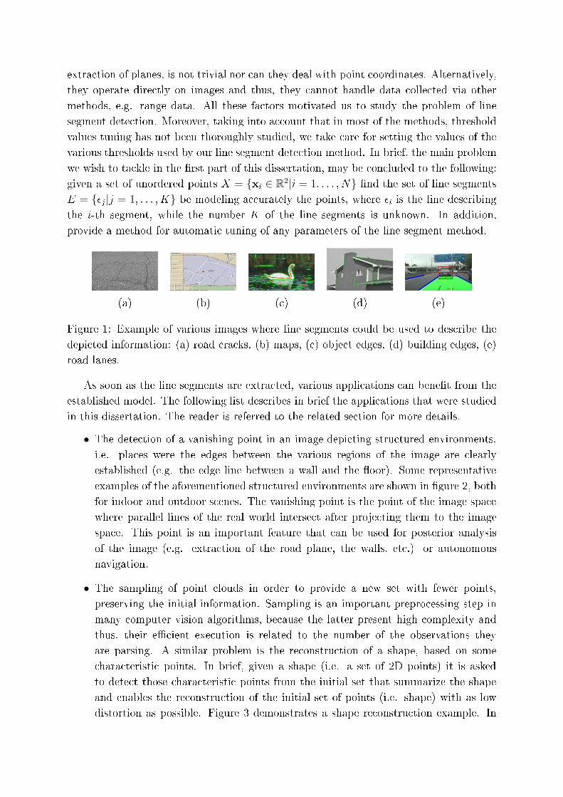
extra tion of planes, is not trivial nor an they deal with point oordinates. Alternatively,

they operate dire tly on images and thus, they annot handle data olle ted via other

methods, e.g. range data. All these fa tors motivated us to study the problem of line

segment dete tion. Moreover, taking into a ount that in most of the methods, threshold

values tuning has not been thoroughly studied, we take are for setting the values of the

various thresholds used by our line segment dete tion method. In brief, the main problem

we wish to ta kle in the �rst part of this dissertation, may be on luded to the following:

given a set of unordered points X = {xi

∈ R2|i = 1; : : : ; N} �nd the set of line segments

E = {�j

|j = 1; : : : ; K} be modeling a urately the points, where �

i

is the line des ribing

the i-th segment, while the number K of the line segments is unknown. In addition,

provide a method for automati tuning of any parameters of the line segment method.

(a) (b) ( ) (d) (e)

Figure 1: Example of various images where line segments ould be used to des ribe the

depi ted information: (a) road ra ks, (b) maps, ( ) obje t edges, (d) building edges, (e)

road lanes.

As soon as the line segments are extra ted, various appli ations an bene�t from the

established model. The following list des ribes in brief the appli ations that were studied

in this dissertation. The reader is referred to the related se tion for more details.

• The dete tion of a vanishing point in an image depi ting stru tured environments,

i.e. pla es were the edges between the various regions of the image are learly

established (e.g. the edge line between a wall and the oor). Some representative

examples of the aforementioned stru tured environments are shown in �gure 2, both

for indoor and outdoor s enes. The vanishing point is the point of the image spa e

where parallel lines of the real world interse t after proje ting them to the image

spa e. This point is an important feature that an be used for posterior analysis

of the image (e.g. extra tion of the road plane, the walls, et .) or autonomous

navigation.

• The sampling of point louds in order to provide a new set with fewer points,

preserving the initial information. Sampling is an important prepro essing step in

many omputer vision algorithms, be ause the latter present high omplexity and

thus, their eÆ ient exe ution is related to the number of the observations they

are parsing. A similar problem is the re onstru tion of a shape, based on some

hara teristi points. In brief, given a shape (i.e. a set of 2D points) it is asked

to dete t those hara teristi points from the initial set that summarize the shape

and enables the re onstru tion of the initial set of points (i.e. shape) with as low

distortion as possible. Figure 3 demonstrates a shape re onstru tion example. In

(a) (b) ( )

Figure 2: Example of images depi ting stru tured worlds. (a) Indoor s ene (b),( ) Out-

door s enes.

�gure 3(a) the initial set is demonstrated, while �gure 3(b) depi ts the extra ted

hara teristi points (green stars). In �gure 3( ) the re onstru tion result is shown

(blue points) superpositioned over the initial shape (red points). Noti e the small

deviation between real and omputed data.

(a) (b) ( )

Figure 3: Example of shape re onstru tion. (a) The initial set of points des ribing a

shape, (b) The hara teristi points (green stars) are extra ted from the initial shape (red

points), ( ) The re onstru tion result (blue points) superpositioned over the initial shape

(red points). Noti e the small deviation between real and omputed data.

• The ompression of bilevel images that depi t the edge map of a real image. More

pre isely, we dealt with the problem of en oding binary images that depi t the

ontour of various shapes. This type of images is mainly used to des ribe obje ts in

the MPEG4 standard, in terms of video en oding. Thus, it is plausible to en ode

individual obje ts in a video frame, a fa t that provides freedom to the end user,

regarding the presentation options. The eÆ ien y of the ompression method is

di tated by the a hieved ompression rate with respe t to distortion.

• The hara terization of a retinal fundus image. The tree stru ture of the veins

in a retinal fundus image an be en oded with line segments. Then it is easy to

dete t the interse tion points of the various veins and pro eed to a post pro essing

algorithm that analyzes this spe ial points.

• A method for extra ting meaningful stru tures in presen e of outliers. In general,

an outlier is onsidered every point that does not obey the general model of the

real data. In other words, as outliers an be onsidered all those points that are

stru tureless, provided that a valid model that des ribes the stru tured data is

established. That model is a set of line segments in our work.

On the other hand, we dealt also with the problem of image and point set registration.

Registration is a very ommon problem and in many ases it is a prepro essing step for

other methods, e.g. the automati evaluation of the development of a patient's ondition

based on the observation of some time varying medi al images. In general, registration

relies on the determination of that parti ular geometri transformation parameter values,

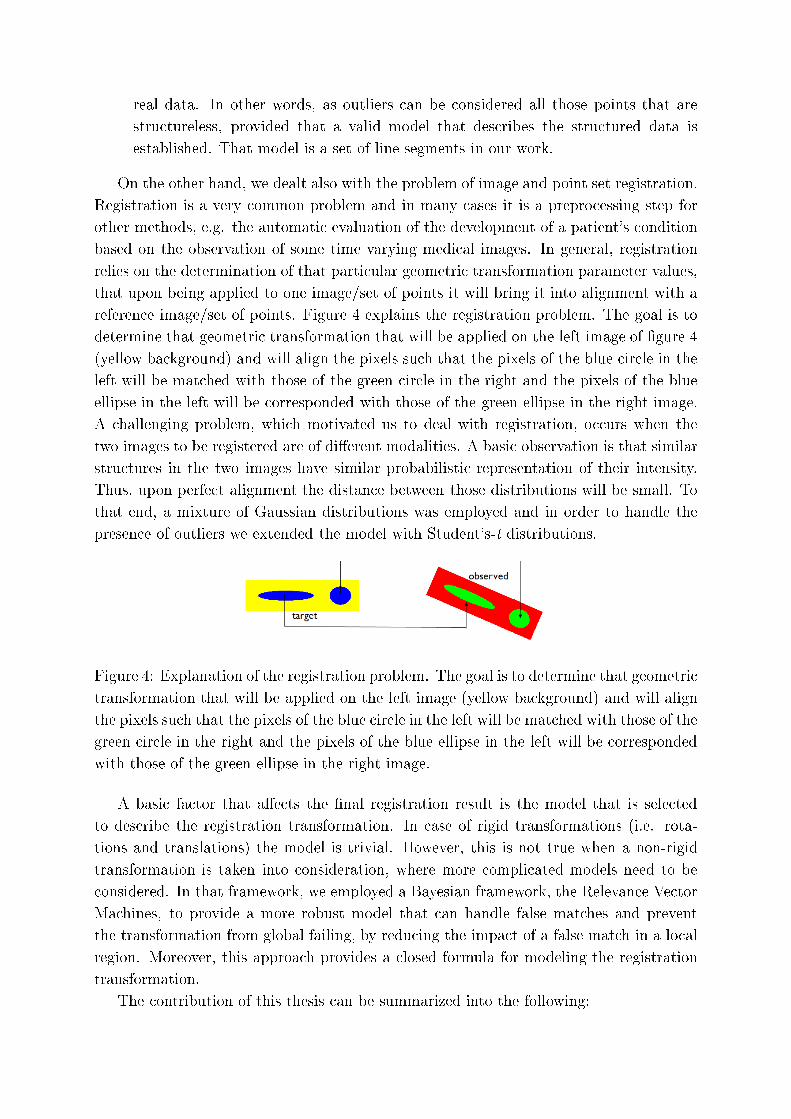
that upon being applied to one image/set of points it will bring it into alignment with a

referen e image/set of points. Figure 4 explains the registration problem. The goal is to

determine that geometri transformation that will be applied on the left image of �gure 4

(yellow ba kground) and will align the pixels su h that the pixels of the blue ir le in the

left will be mat hed with those of the green ir le in the right and the pixels of the blue

ellipse in the left will be orresponded with those of the green ellipse in the right image.

A hallenging problem, whi h motivated us to deal with registration, o urs when the

two images to be registered are of di�erent modalities. A basi observation is that similar

stru tures in the two images have similar probabilisti representation of their intensity.

Thus, upon perfe t alignment the distan e between those distributions will be small. To

that end, a mixture of Gaussian distributions was employed and in order to handle the

presen e of outliers we extended the model with Student's-t distributions.

Figure 4: Explanation of the registration problem. The goal is to determine that geometri

transformation that will be applied on the left image (yellow ba kground) and will align

the pixels su h that the pixels of the blue ir le in the left will be mat hed with those of the

green ir le in the right and the pixels of the blue ellipse in the left will be orresponded

with those of the green ellipse in the right image.

A basi fa tor that a�e ts the �nal registration result is the model that is sele ted

to des ribe the registration transformation. In ase of rigid transformations (i.e. rota-

tions and translations) the model is trivial. However, this is not true when a non-rigid

transformation is taken into onsideration, where more ompli ated models need to be

onsidered. In that framework, we employed a Bayesian framework, the Relevan e Ve tor

Ma hines, to provide a more robust model that an handle false mat hes and prevent

the transformation from global failing, by redu ing the impa t of a false mat h in a lo al

region. Moreover, this approa h provides a losed formula for modeling the registration

transformation.

The ontribution of this thesis an be summarized into the following:

• An iterative framework for line segment dete tion to summarize unordered point

sets.

• A voting s heme for the dete tion of vanishing points in stru tured images.

• A method for eÆ iently annotating retinal fundus images.

• A method for eÆ iently sampling unordered 2D points.

• A omparative study between line segment extra tion methods for bilevel image

ompression.

• A method for extra ting stru tures (e.g. shapes) in presen e of outliers.

• A Bayesian approa h for modeling a non-rigid registration transformation whi h is

robust to false mat hes.

• An algorithm for registering multimodal images and loud of points.

0.2 Stru ture of the thesis

The �rst part of this thesis deals with line segment extra tion from a set of unordered

points and appli ations. The se ond part presents our work in the �eld of image and

point set registration.

In Chapter 1, we introdu e an iterative method for the extra tion of line segments.

A short introdu tion of the related literature is provided and the proposed algorithm is

des ribed in detail. Finally, an extensive experimental evaluation is provided omparing

our method with other ommonly used approa hes.

In Chapter 2, some appli ations based on line segment dete tion are introdu ed.

A short introdu tion is presented for ea h appli ation, to des ribe the problem and the

various solutions provided in the related literature. Then, the proposed method is pre-

sented along with an experimental evaluation and omparison with the state-of-the-art.

Thus, se tion 2.1 deals with the dete tion of the vanishing point in stru tured images,

se tion 2.2 presents an eÆ ient algorithm for sampling unordered points, in se tion

2.3 a method for shape en oding and bilevel image ompression is presented, in se tion

2.4 a method for hara terizing a retinal fundus image is demonstrated, and �nally, in

se tion 2.5 an algorithm for extra ting stru tured information (e.g. shapes) in presen e

of outliers is introdu ed.

In Chapter 3, the modeling of a non rigid transformation for point set registration

is presented. The algorithm is des ribed in detail and various experimental results are

demonstrated.

In Chapter 4, we des ribe a solution of the rigid registration problem based on

mixture models.

Part I

Features and Appli ations

Chapter 1

Modeling sets of unordered points

using line segments

1.1 Introdu tion

1.2 A Dire t Split and Merge (DSaM) Framework for Line Segment Dete tion

1.2.1 Split pro ess

1.2.2 Merge pro ess

1.3 Evaluation of the Line Segment Dete tion Algorithm

1.3.1 Numeri al Evaluation

1.3.2 Comparison with the Hough Transform

1.1 Introdu tion

Lines are one of the most basi models to des ribe features in an image due to their

simpli ity, regarding the modeling parameters. Moreover, lines are suitable models for

des ribing real world stru tures as most of the human made s enes are being represented

by at surfa es. Lines an be used to summarize features in a higher level, e.g. ontours.

Examples regarding the importan e of line extra tion in lude the dete tion of vanish-

ing points [18℄, the ve torization of raster images [19℄ and the dete tion of road stru tures

and parts [20℄ are among appli ations ne essitating line segment des ription of image

stru tures. In many of the aforementioned problems, the involved algorithms assume

that they are provided with an ordered point set and standard polygonal approximation

[10, 21℄ is then applied. However, determining the ordering of point sets is not a trivial

task and in the method des ribed herein we relax this assumption by making no prior

hypothesis about the ordering of the points.

1

In the above ontext, the Hough transform (HT) is a widely used method for line

�tting and many variants have been proposed to improve its eÆ ien y [22, 23℄. One of

these variants is the randomized Hough transform (RHT) [24, 25℄ whi h randomly sele ts

a number of pixels from the input image and maps them into one point in the parameter

spa e whi h was shown to be less omplex, ompared to the original algorithm, as far

as time and storage issues are on erned. In [26℄, the probabilisti HT was proposed

whose basi idea is to apply a random sampling of edge points to redu e omputational

omplexity and exe ution time. Further improvements were introdu ed in [27℄. A similar

on ept was proposed in [28℄, where an orientation-based strategy was adopted to �lter

out inappropriate edge pixels, before performing the standard HT line dete tion whi h

improves the randomized dete tion pro ess. Also, the idea of fuzziness is integrated in

the main algorithm in [29℄ to model the un ertainty imposed to the ontour due to noise.

Thus, a point an ontribute to more than one bin in the standard HT pro ess. A general

omparison between probabilisti and non-probabilisti HT variants an be found in [30℄.

The robust HT is introdu ed in [31℄ where both the length and the end points of the

lines may be omputed. Moreover, the algorithm in [32℄ provides a method for adopting a

shape dependent voting s heme for the al ulation of the histogram bins. Finally, a novel

HT based on the eliminating parti le swarm optimization (EPSO) is proposed in [33℄,

to improve the exe ution time of the algorithm. The problem parameters are onsidered

to be the parti le positions and the EPSO algorithm sear hes the optimum solution by

eliminating the "weakest" parti les, to speed up the pro ess.

Line segment �tting may also be used in a shape des ription pro ess. The ommonly

used algorithm of Moore [34℄ was a �rst solution to shape following and utilizes the

neighborhood of points. However, this algorithm is appropriate only for traversing urves

without interse tions and produ es models with high omplexity, although improvements

of the main algorithm have also been onsidered up to date [35℄. Another ommon model

�tting method is the RANSAC algorithm [36℄, whi h despite the fa t that it provides

robust estimations, it is appropriate for �tting only one model at a time. Other approa hes

are the in remental line �tting [37℄ whi h is sensitive to noise and, most importantly, needs

sequential ordering of the points and probabilisti methods [38℄ based on the Expe tation-

Maximization algorithm, generally ne essitating the prior determination of the number

of model omponents.

More re ently a new method was introdu ed that relies on the Helmholtz prin iple: 'no

stru ture is per eived in white noise', based on the work of [39℄ for adaptive thresholding.

Its main hara teristi , a ording to the authors, is that this method is parameterless and

an a urately ontrol the false positive and false negative dete tions. In brief, initially

the image gradient is omputed at ea h pixel and then through a region growing algo-

rithm they try to align points whose gradient dire tion is within a prede�ned threshold.

Although that there is a threshold parameter, the authors laim that their method is

nearly parameterless be ause the de ision threshold on the number of ontrol points in a

given segment is in a

√

( log) dependen y of the expe ted number of false alarms. The

2

reader is refereed to [40, 41℄ for more details and to [42℄ for the implementation details of

the method.

1.2 A Dire t Split and Merge (DSaM) Framework for Line Seg-

ment Dete tion

Let X = {xi

|i = 1; : : : ; N} be a set of points and E = {�j

|j = 1; : : : ; K} be the set of linesegments modeling the points, where �

i

is the line des ribing the i-th segment.

We de�ne the modeling error ∆ indu ed by the representation of line segments:

∆(X;E) =N∑

i=1

K∑

j=1

Æ

ij

d(xi

; �

j

); (1.1)

where K is the number of line segments the model uses to model the points, x

i

∈ R2,

i = 1; : : : ; N are the points, d(xi

; �

j

) is the perpendi ular distan e of point xi

to line �

j

,

Æ

ij

is an indi ator fun tion whose value is one if point x

i

belongs to line segment �

j

and

is zero otherwise.

In order to prevent over�tting, models having a large number of line segments should

be penalized. Therefore, an optimal model would have both low value of ∆ and low

omplexity.

The omputation of the ellipses, modeling the line segments, is performed in two steps:

an iterative split pro ess, where points are modeled by a number of line segments repre-

sented by the major axes of the orresponding ellipses and an iterative merge pro ess,

where small line segments are merged to redu e the model omplexity. The split pro ess

tries to minimize the modeling error while the merge pro ess de reases the model om-

plexity, i.e. the number of line segments ompared to the total number of points in the

set.

In what follows the two steps are presented in detail.

1.2.1 Split Pro ess

The ultimate goal of this step is to over the point spa e with line segments representing

the long axes of elongated ellipses and therefore, ea h point of the shape should be assigned

to an e entri ellipse. A split riterion is de�ned, based on Gestalt theory [43℄, whi h

models the linearity and the onne tivity the human brain uses when modeling ontours.

In order to split a set X, it should be either non linear or dis onne ted, or both. Lin-

earity des ribes how lose the points are to a straight line, while dis onne tivity measures

how on entrated these points are. In the ideal ase, the ovarian e matrix of ollinear

2D points should have a very large eigenvalue and a zero eigenvalue. The eigenve tor

orresponding to the larger eigenvalue indi ates the dire tion of the line segment. If the

linearity property is relaxed, the less ollinear the points be ome (i.e. they diverge from

the linear assumption) the larger the value of the minimum eigenvalue is. Based on that

3

observation, in our method, linearity is des ribed by the minimum eigenvalue of the o-

varian e matrix of the points in X. Also, the dis onne tivity W of two sets of points X,

Y is the smallest distan e between a point in X and a point in Y :

W (X; Y ) = minx∈Xy∈Y

|x− y|: (1.2)

In the ase of a single set, dis onne tivity is the largest distan e between two su essive

points in that set. It may be omputed by proje ting the points onto both axes de�ned by

the eigenve tors of the ovarian e matrix of the set. Then, su essive points are de�ned

by s anning along the axes and their distan es are omputed. Let X

i

be the proje tion

of a set X onto the the eigenve tor e

i

. The dis onne tivity of X is de�ned as

W (X) = maxj=1;:::;N−1i=1;:::;d

|xji

− x

j+1i

|; (1.3)

where N is the number of points inX, d is the dimension ofX (here d = 2) and xji

is the j-

th point of the sorted set X

i

. A large value of dis onne tivity indi ates a better separation

of the point sets. The proje tions onto all of the eigenve tors should be examined as we

do not know a priori whi h dire tion to follow while splitting. Although intuitively one

would suggest to split along the dire tion of the prin ipal axis, we observed that in many

ases that approa h was not the best. Also, let us note that as the ordering of the points

is not known a priori, their proje tion onto the eigenve tors of their ovarian e matrix,

provides a natural way of ordering.

The dis onne tivity of a single set of points is also important to be estimated in the

split step, as there may exist subsets that although they are linear, they are dis onne ted.

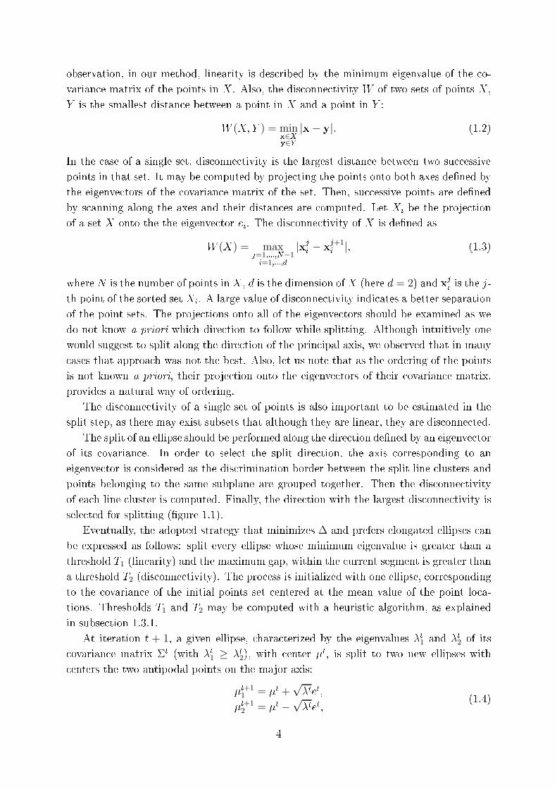
The split of an ellipse should be performed along the dire tion de�ned by an eigenve tor

of its ovarian e. In order to sele t the split dire tion, the axis orresponding to an

eigenve tor is onsidered as the dis rimination border between the split line lusters and

points belonging to the same subplane are grouped together. Then the dis onne tivity

of ea h line luster is omputed. Finally, the dire tion with the largest dis onne tivity is

sele ted for splitting (�gure 1.1).

Eventually, the adopted strategy that minimizes ∆ and prefers elongated ellipses an

be expressed as follows: split every ellipse whose minimum eigenvalue is greater than a

threshold T1 (linearity) and the maximum gap, within the urrent segment is greater than

a threshold T2 (dis onne tivity). The pro ess is initialized with one ellipse, orresponding

to the ovarian e of the initial points set entered at the mean value of the point lo a-

tions. Thresholds T1 and T2 may be omputed with a heuristi algorithm, as explained

in subse tion 1.3.1.

At iteration t + 1, a given ellipse, hara terized by the eigenvalues �

t

1 and �

t

2 of its

ovarian e matrix Σt

(with �

t

1 ≥ �

t

2), with enter �

t

, is split to two new ellipses with

enters the two antipodal points on the major axis:

�

t+11 = �

t +√�

t

e

t

,

�

t+12 = �

t −√�

t

e

t

,

(1.4)

4

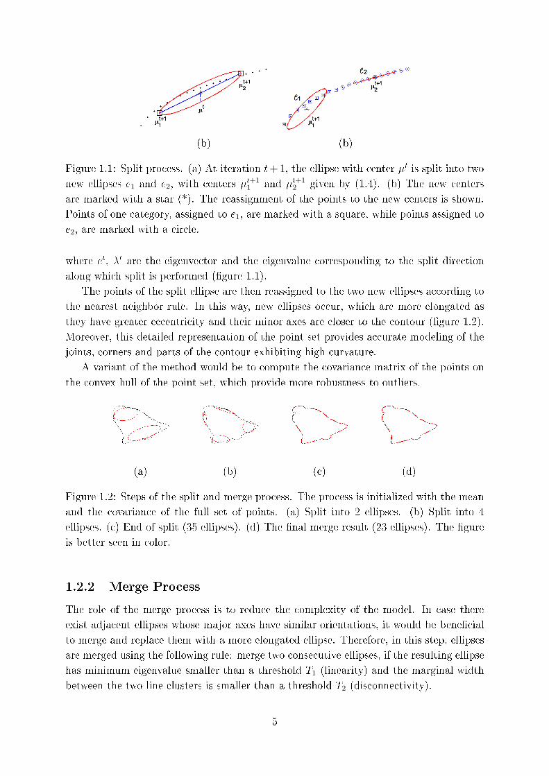
(b) (b)

Figure 1.1: Split pro ess. (a) At iteration t+1, the ellipse with enter �

t

is split into two

new ellipses e1 and e2, with enters �

t+11 and �

t+12 given by (1.4). (b) The new enters

are marked with a star (*). The reassignment of the points to the new enters is shown.

Points of one ategory, assigned to e1, are marked with a square, while points assigned to

e2, are marked with a ir le.

where e

t

, �

t

are the eigenve tor and the eigenvalue orresponding to the split dire tion

along whi h split is performed (�gure 1.1).

The points of the split ellipse are then reassigned to the two new ellipses a ording to

the nearest neighbor rule. In this way, new ellipses o ur, whi h are more elongated as

they have greater e entri ity and their minor axes are loser to the ontour (�gure 1.2).

Moreover, this detailed representation of the point set provides a urate modeling of the

joints, orners and parts of the ontour exhibiting high urvature.

A variant of the method would be to ompute the ovarian e matrix of the points on

the onvex hull of the point set, whi h provide more robustness to outliers.

(a) (b) ( ) (d)

Figure 1.2: Steps of the split and merge pro ess. The pro ess is initialized with the mean

and the ovarian e of the full set of points. (a) Split into 2 ellipses. (b) Split into 4

ellipses. ( ) End of split (35 ellipses). (d) The �nal merge result (23 ellipses). The �gure

is better seen in olor.

1.2.2 Merge Pro ess

The role of the merge pro ess is to redu e the omplexity of the model. In ase there

exist adja ent ellipses whose major axes have similar orientations, it would be bene� ial

to merge and repla e them with a more elongated ellipse. Therefore, in this step, ellipses

are merged using the following rule: merge two onse utive ellipses, if the resulting ellipse

has minimum eigenvalue smaller than a threshold T1 (linearity) and the marginal width

between the two line lusters is smaller than a threshold T2 (dis onne tivity).

5

Note that the threshold T1 ould be set equal to the threshold used in the split pro ess,

where the value of parameter T1 spe i�es whether an ellipse has low e entri ity and needs

to be split. In the merge pro ess, it indi ates whether two andidates for merging ellipses

would result in an ellipse with high e entri ity. One ould use the same threshold in

both pro esses, assuming the same signi� an e. On the other hand, a relaxation of the

merge threshold ould lead to a rougher model of the points, smoothing out details like

joints. In our experiments, the merge threshold was sele ted to be the same with the split

threshold. The same applies for threshold T2 that indi ates whether two segments are

lose enough to be onsidered as one line segment.

The overall des ription of the method is presented in Algorithm 1.

SPLIT PROCESS

input: The set of points X = {xi

|i = 1; : : : ; N}.output: A set of ellipses {�

j

;Σj

}.Initialize the algorithm by estimating the mean and ovarian e of the point lo ations.

while there are ellipses to split do

Split every ellipse whose minor eigenvalue is greater than T1 and its dis onne tivity

is greater than T2.

• Sele t the dire tion that provides the greatest dis onne tivity.

• Set the enters of the new ellipses a ording to (1.4).

MERGE PROCESS

input: The ellipses from the split pro ess �

j

= {�j

;Σj

}; j = 1; : : : ;M .

output: A redu ed set of ellipses.

while there are ellipses to merge do

for all ellipses �

i

; i = 1; : : : ;M do

if merging �

i

with �

j

provides an ellipse whose minor eigenvalue is less than T1

and its dis onne tivity is less than T2 then

A ept merging.

Set �

i

to the ellipse that result from merging

Algorithm 1: Dire t Split-and-Merge Algorithm

1.3 Evaluation of the Line Segment Dete tion Algorithm

In this se tion we evaluate the eÆ ien y of the introdu ed algorithm. To that end, two at-

egories of experiments were ondu ted. The purpose was to investigate the performan e

of the method both in shape data, but also in real images. Thus, various well-known

databases were employed, that ontain either obje t silhouettes or s enes of real images.

6

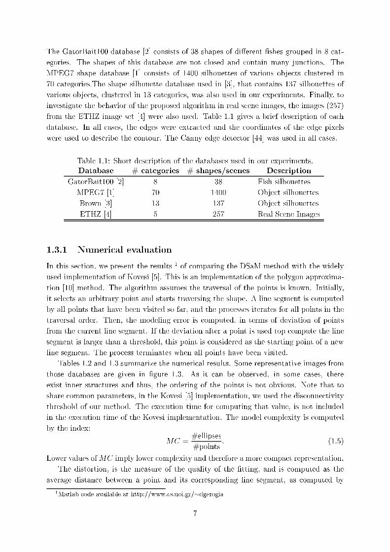
The GatorBait100 database [2℄ onsists of 38 shapes of di�erent �shes grouped in 8 at-

egories. The shapes of this database are not losed and ontain many jun tions. The

MPEG7 shape database [1℄ onsists of 1400 silhouettes of various obje ts lustered in

70 ategories.The shape silhouette database used in [3℄, that ontains 137 silhouettes of

various obje ts, lustered in 13 ategories, was also used in our experiments. Finally, to

investigate the behavior of the proposed algorithm in real s ene images, the images (257)

from the ETHZ image set [4℄ were also used. Table 1.1 gives a brief des ription of ea h

database. In all ases, the edges were extra ted and the oordinates of the edge pixels

were used to des ribe the ontour. The Canny edge dete tor [44℄ was used in all ases.

Table 1.1: Short des ription of the databases used in our experiments.

Database # ategories # shapes/s enes Des ription

GatorBait100 [2℄ 8 38 Fish silhouettes

MPEG7 [1℄ 70 1400 Obje t silhouettes

Brown [3℄ 13 137 Obje t silhouettes

ETHZ [4℄ 5 257 Real S ene Images

1.3.1 Numeri al evaluation

In this se tion, we present the results

1

of omparing the DSaM method with the widely

used implementation of Kovesi [5℄. This is an implementation of the polygon approxima-

tion [10℄ method. The algorithm assumes the traversal of the points is known. Initially,

it sele ts an arbitrary point and starts traversing the shape. A line segment is omputed

by all points that have been visited so far, and the pro esses iterates for all points in the

traversal order. Then, the modeling error is omputed, in terms of deviation of points

from the urrent line segment. If the deviation after a point is used top ompute the line

segment is larger than a threshold, this point is onsidered as the starting point of a new

line segment. The pro ess terminates when all points have been visited.

Tables 1.2 and 1.3 summarize the numeri al results. Some representative images from

those databases are given in �gure 1.3. As it an be observed, in some ases, there

exist inner stru tures and thus, the ordering of the points is not obvious. Note that to

share ommon parameters, in the Kovesi [5℄ implementation, we used the dis onne tivity

threshold of our method. The exe ution time for omputing that value, is not in luded

in the exe ution time of the Kovesi implementation. The model omplexity is omputed

by the index:

MC =#ellipses

#points

: (1.5)

Lower values ofMC imply lower omplexity and therefore a more ompa t representation.

The distortion, is the measure of the quality of the �tting, and is omputed as the

average distan e between a point and its orresponding line segment, as omputed by

1

Matlab ode available at http://www. s.uoi.gr/∼dgerogia

7

(a) (b) ( ) (d)

Figure 1.3: Some representative images of the databases we used in our experiments.

Please note that in some ases inner stru tures exist. This does not permit to extra t an

ordering of the points (a)MPEG7 [1℄, (b) Gatorbait [2℄, ( ) Brown [3℄, (d) ETHZ [4℄.

Table 1.2: Modeling Error ∆ (1.1)

MPEG7 [1℄ (70 shapes)

method mean std median min max

DSaM 0.489 0.093 0.509 0.080 0.773

Kovesi 2.796 3.977 1.736 0.533 46.984

GatorBait100 [2℄ (38 shapes)


DSaM 0.454 0.033 0.452 0.383 0.509

Kovesi 2.215 0.862 1.981 1.477 6.473

Brown [3℄ (137 shapes)


DSaM 0.492 0.119 0.514 0.105 0.894

Kovesi 2.871 6.192 1.095 0.617 33.632

ETHZ [4℄ (255 s enes)


DSaM 0.494 0.061 0.503 0.257 0.635

Kovesi 2.299 1.340 1.914 1.056 12.655

8

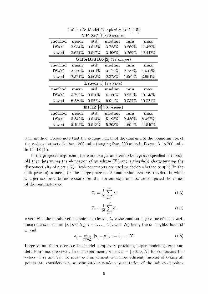
Table 1.3: Model Complexity MC (1.5)



DSaM 3.954% 0.013% 3.788% 0.269% 11.429%

Kovesi 3.624% 0.017% 3.406% 0.269% 12.442%



DSaM 3.280% 0.004% 3.172% 2.732% 4.541%

Kovesi 2.524% 0.005% 2.378% 1.961% 3.904%

Brown [3℄ (7 s enes)


DSaM 5.792% 0.016% 6.186% 0.921% 10.145%

Kovesi 6.586% 0.022% 6.911% 0.335% 10.821%

ETHZ [4℄ (16 s enes)


DSaM 5.342% 0.014% 5.195% 2.436% 8.427%

Kovesi 5.402% 0.018% 5.205% 1.601% 11.040%

ea h method. Please note that the average length of the diagonal of the bounding box of

the various datasets, is about 500 units (ranging from 300 units in Brown [3℄ to 700 units

in ETHZ [4℄).

In the proposed algorithm, there are two parameters to be a priori spe i�ed, a thresh-

old that determines the elongation of an ellipse (T1) and a threshold hara terizing the

dis onne tivity of a set (T2). Both parameters are used to de ide whether to split (in the

split pro ess) or merge (in the merge pro ess). A small value preserves the details, while

a larger one provides more oarse results. For our experiments, we omputed the values

of the parameters as:

T1 =1

N

N∑

i=1

�

i

(1.6)

T2 =1

N

N∑

i=1

d

i

(1.7)

where N is the number of the points of the set, �

i

is the smallest eigenvalue of the ovari-

an e matrix of points {x |x ∈ N

�

x

i

; i = 1; : : : ; N}, with N�

x

being the �- neighborhood of

x, and

d

i

= miny∈N�

x

i

||xi

− y||; i = 1; : : : ; N: (1.8)

Large values for � de rease the model omplexity providing larger modeling error and

details are not preserved. In our experiments, we set � = ⌈0:01 × N⌉ for omputing the

values of T1 and T2. To make our implementation more eÆ ient, instead of taking all

points into onsideration, we omputed a random permutation of the indi es of points

9

and used only the �rst 10% of them. Thus, in high density datasets, like in the ETHZ

database [4℄, the values of the thresholds ould be estimated qui kly.

In general, the DSaM method and the Kovesi implementation produ e models with

similar omplexity, a fa t that is obvious, sin e they employ the same thresholds. However,

the DSaM method provides mu h more a urate results w.r.t distortion (Table 1.2 and

Table 1.3).

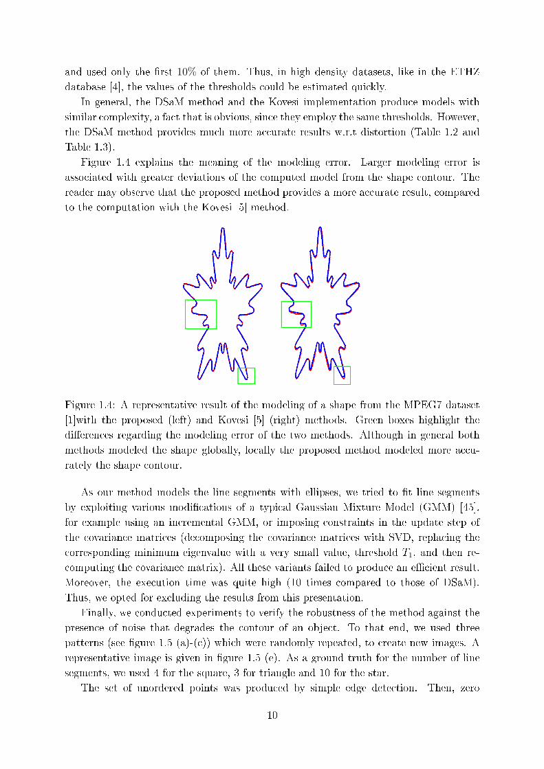
Figure 1.4 explains the meaning of the modeling error. Larger modeling error is

asso iated with greater deviations of the omputed model from the shape ontour. The

reader may observe that the proposed method provides a more a urate result, ompared

to the omputation with the Kovesi [5℄ method.

Figure 1.4: A representative result of the modeling of a shape from the MPEG7 dataset

[1℄with the proposed (left) and Kovesi [5℄ (right) methods. Green boxes highlight the

di�eren es regarding the modeling error of the two methods. Although in general both

methods modeled the shape globally, lo ally the proposed method modeled more a u-

rately the shape ontour.

As our method models the line segments with ellipses, we tried to �t line segments

by exploiting various modi� ations of a typi al Gaussian Mixture Model (GMM) [45℄,

for example using an in remental GMM, or imposing onstraints in the update step of

the ovarian e matri es (de omposing the ovarian e matri es with SVD, repla ing the

orresponding minimum eigenvalue with a very small value, threshold T1, and then re-

omputing the ovarian e matrix). All these variants failed to produ e an eÆ ient result.

Moreover, the exe ution time was quite high (10 times ompared to those of DSaM).

Thus, we opted for ex luding the results from this presentation.

Finally, we ondu ted experiments to verify the robustness of the method against the

presen e of noise that degrades the ontour of an obje t. To that end, we used three

patterns (see �gure 1.5 (a)-( )) whi h were randomly repeated, to reate new images. A

representative image is given in �gure 1.5 (e). As a ground truth for the number of line

segments, we used 4 for the square, 3 for triangle and 10 for the star.

The set of unordered points was produ ed by simple edge dete tion. Then, zero

10

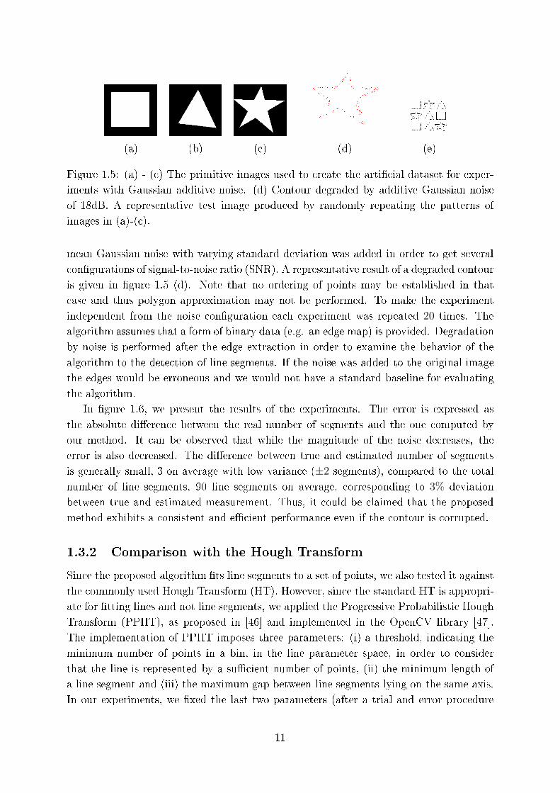
(a) (b) ( ) (d) (e)

Figure 1.5: (a) - ( ) The primitive images used to reate the arti� ial dataset for exper-

iments with Gaussian additive noise. (d) Contour degraded by additive Gaussian noise

of 18dB. A representative test image produ ed by randomly repeating the patterns of

images in (a)-( ).

mean Gaussian noise with varying standard deviation was added in order to get several

on�gurations of signal-to-noise ratio (SNR). A representative result of a degraded ontour

is given in �gure 1.5 (d). Note that no ordering of points may be established in that

ase and thus polygon approximation may not be performed. To make the experiment

independent from the noise on�guration ea h experiment was repeated 20 times. The

algorithm assumes that a form of binary data (e.g. an edge map) is provided. Degradation

by noise is performed after the edge extra tion in order to examine the behavior of the

algorithm to the dete tion of line segments. If the noise was added to the original image

the edges would be erroneous and we would not have a standard baseline for evaluating

the algorithm.

In �gure 1.6, we present the results of the experiments. The error is expressed as

the absolute di�eren e between the real number of segments and the one omputed by

our method. It an be observed that while the magnitude of the noise de reases, the

error is also de reased. The di�eren e between true and estimated number of segments

is generally small, 3 on average with low varian e (±2 segments), ompared to the total

number of line segments, 90 line segments on average, orresponding to 3% deviation

between true and estimated measurement. Thus, it ould be laimed that the proposed

method exhibits a onsistent and eÆ ient performan e even if the ontour is orrupted.

1.3.2 Comparison with the Hough Transform

Sin e the proposed algorithm �ts line segments to a set of points, we also tested it against

the ommonly used Hough Transform (HT). However, sin e the standard HT is appropri-

ate for �tting lines and not line segments, we applied the Progressive Probabilisti Hough

Transform (PPHT), as proposed in [46℄ and implemented in the OpenCV library [47℄.

The implementation of PPHT imposes three parameters: (i) a threshold, indi ating the

minimum number of points in a bin, in the line parameter spa e, in order to onsider

that the line is represented by a suÆ ient number of points, (ii) the minimum length of

a line segment and (iii) the maximum gap between line segments lying on the same axis.

In our experiments, we �xed the last two parameters (after a trial and error pro edure

11

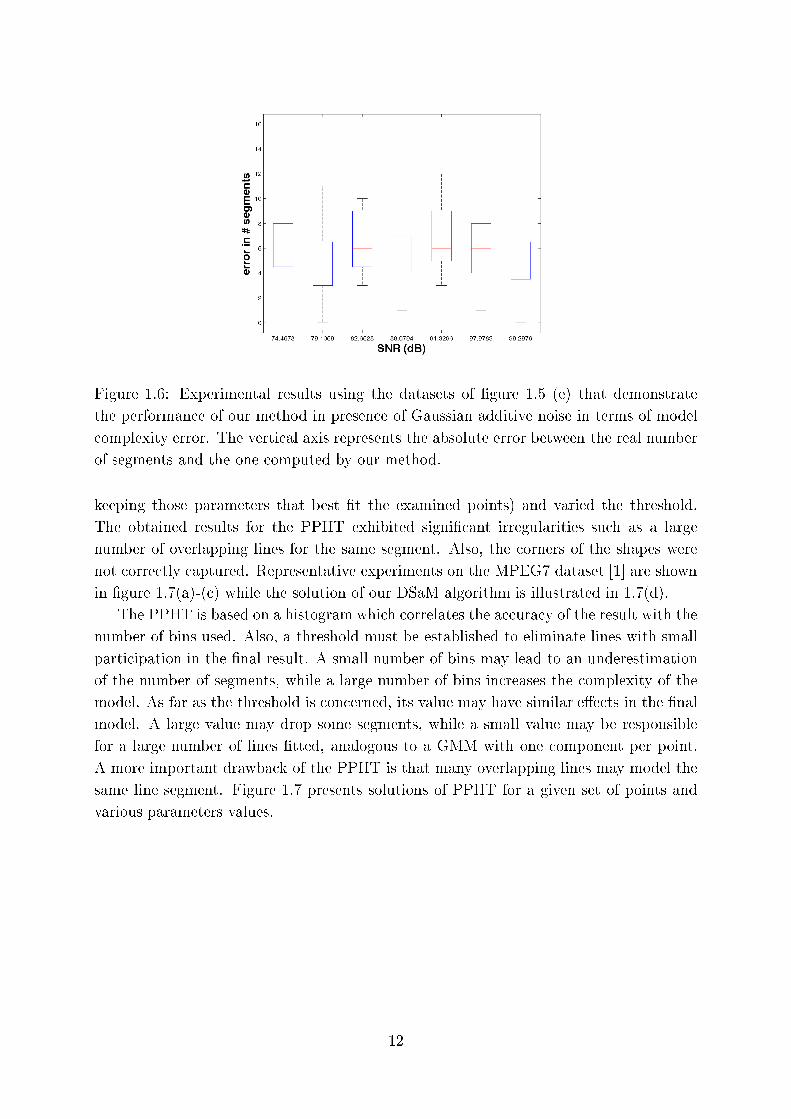
Figure 1.6: Experimental results using the datasets of �gure 1.5 (e) that demonstrate

the performan e of our method in presen e of Gaussian additive noise in terms of model

omplexity error. The verti al axis represents the absolute error between the real number

of segments and the one omputed by our method.

keeping those parameters that best �t the examined points) and varied the threshold.

The obtained results for the PPHT exhibited signi� ant irregularities su h as a large

number of overlapping lines for the same segment. Also, the orners of the shapes were

not orre tly aptured. Representative experiments on the MPEG7 dataset [1℄ are shown

in �gure 1.7(a)-( ) while the solution of our DSaM algorithm is illustrated in 1.7(d).

The PPHT is based on a histogram whi h orrelates the a ura y of the result with the

number of bins used. Also, a threshold must be established to eliminate lines with small

parti ipation in the �nal result. A small number of bins may lead to an underestimation

of the number of segments, while a large number of bins in reases the omplexity of the

model. As far as the threshold is on erned, its value may have similar e�e ts in the �nal

model. A large value may drop some segments, while a small value may be responsible

for a large number of lines �tted, analogous to a GMM with one omponent per point.

A more important drawba k of the PPHT is that many overlapping lines may model the

same line segment. Figure 1.7 presents solutions of PPHT for a given set of points and

various parameters values.

12

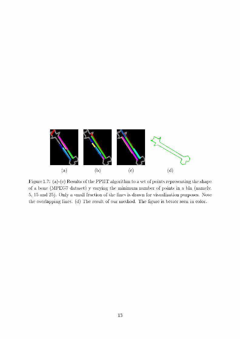
(a) (b) ( ) (d)

Figure 1.7: (a)-( ) Results of the PPHT algorithm to a set of points representing the shape

of a bone (MPEG7 dataset) y varying the minimum number of points in a bin (namely,

5, 15 and 25). Only a small fra tion of the lines is drawn for visualization purposes. Note

the overlapping lines. (d) The result of our method. The �gure is better seen in olor.

13

Chapter 2

Appli ations

2.1 Vanishing Point Dete tion

2.1.1 Introdu tion

2.1.2 The algorithm


2.2 Point loud sampling and re onstru tion

2.2.1 Introdu tion

2.2.2 The algorithm


2.3 Shape en oding for edge map image ompression

2.3.1 Introdu tion

2.3.2 The algorithm


2.4 Retinal Fundus Image Feature Chara terization

2.4.1 Introdu tion

2.4.2 The algorithm


2.5 Elimination of outliers from 2D point sets using the Helmholtz prin iple

2.5.1 Introdu tion

2.5.2 The Helmholtz prin iple

2.5.3 The algorithm


14

2.1 Vanishing Point Dete tion

2.1.1 Introdu tion

Human-made s enes, su h as roads, buildings and their fa ades or indoor orridor bound-

aries have a large number of parallel lines in the 3D spa e. In the framework of a pinhole

amera model, two parallel lines are proje ted onto a pair of onverging lines in the 2D

image spa e provided that their 3D plane is not fronto-parallel to the image plane. The

ommon point of interse tion of all 3D parallel lines (generally belonging to di�erent

planes) in the 2D image is alled the vanishing point. The dete tion of a vanishing point

in an image is a ru ial step in many omputer vision appli ations, like robot navigation,

amera alibration, single view 3D s ene re onstru tion and pose estimation.

In the related literature, there are two main ategories of methods for vanishing point

dete tion. There are te hniques requiring knowledge of the intrinsi parameters of the

amera, whi h exploit the notion of 3D parallelism and prominent stru tures of the s ene

orthogonal to ea h other, also alled Manhattan dire tions [48, 49℄. There are also te h-

niques assuming no knowledge of the internal amera parameters, su h as the method in

[50℄ using the Helmholtz prin iple for image partitioning, the Expe tation-Maximization

(EM) framework adopted in [51℄ or the non-iterative algorithm based on onsensus sets

[52℄.

In ontrast to the above methods, whi h may base their estimation in the existen e

of three orthogonal vanishing points, images a quired in stru tured environments su h as

roads or orridors are a spe i� ategory where the dete tion of a single vanishing point

may be suÆ ient for the underlined appli ation (e.g. vision-based robot motion along a

orridor). The general strategy onsists in partitioning the image into a umulator ells

olle ting votes from the line segments having their interse tion in the spe i� ell. The

dete tion of peaks in the a umulator spa e provides the vanishing points [53, 54℄.

An alternative approa h is presented in that hapter, based on the DSaM algorithm of

hapter 1. Se ondly, a voting step is applied through a kernel, where andidate vanishing

points are assigned weights proportional to the lengths of the line segments they belong

to. Therefore, longer line segments whi h are more probable in indoor environments (e.g.

the interse tion of wall and ground) are more probable to ontribute to the determination

of the vanishing point.

2.1.2 The algorithm

Given an indoor s ene (e.g. a orridor), the �rst step of the method onsists in dete ting

the edges of the image. Therefore, the probabilisti boundaries are �rst omputed [55℄

though in simpler, non textured environments, the output of the standard but established

Canny edge dete tor dete tor [44℄ is generally a eptable. Then the DSaM algorithm is

performed to model the s enes line segments. Please note that other methods may also

be applied.

15

The next step onsists in �tting line segments to the extra ted edges. Various algo-

rithms may be employed, like the one des ribed in 1.

After the determination of the line segments in terms of the long axes of highly e -

entri ellipses, the set Cvp

of andidate vanishing points is onstru ted by omputing all

the pairwise interse tion points between all the lines. To further improve the eÆ ien y

of the method, interse tion points that lie outside the image plane ould be ignored but

this issue is optional and depends on the spe i� appli ation. For example, in a orridor,

the vanishing point lies within the image plain and intuitively the vanishing line usually

appears somewhere in the viewer's horizon. On the other hand, if the algorithm is to be

used by a robot navigation system, the dete tion of the vanishing point outside the image

plane may indi ate an abrupt turn.

Then e, a weight w(p) = |lp1 ||lp2 | is assigned to ea h point p ∈ Cvp

whi h is equal

to the produ t of the lengths |lp1 | and |lp2 | of the two line segments whose interse tion is

the andidate vanishing point p. Thus, a andidate vanishing point produ ed by short

segments, or one long and one short segment, is attributed with a small weight.

In the �nal step of our work ow, the vanishing point is omputed by sele ting one of

the andidate points, whi h is a hieved through a voting s heme. This step is similar in

spirit to the approa h presented in [53℄. However, the main di�eren e with respe t to that

method is that, in our algorithm, ea h line segment votes only for the interse tion points

belonging to it while in [53℄ a line segment votes for every andidate vanishing point (even

if it does not belong to the segment).

In a voting s heme, an important fa tor is the size of the a umulator array bins,

whi h in our ase is a grid overing the image support G ≡ [0, Gw

] × [0, Gh

] ⊂ R2. The

grid is uniformly divided into equally sized ells B

i

, i = 1; :::; N , using a s aling fa tor

� ∈ (0; 1] imposing a bin size of [�Gw

; �G

h

].

In order to assign weights to ea h andidate vanishing point present in a given bin,

a kernel fun tion entered at ea h array bin is employed. To this end, a 2D Π-Sigmoid

kernel is applied to ea h bin [56℄, imposing thus a fuzzy on ept to the borders of the ell.

The support of a 1D Π-Sigmoid kernel:

k(x) =1

b− a

[1

1 + e

−�(x−a)− 1

1 + e

−�(x−b)

]

; (2.1)

with � > 0, whi h is depi ted in �gure 2.1, approximates a uniform kernel whose borders

are fuzzi�ed in order to avoid abrupt hanges. Thus, points under the plateau ontribute

equally with their votes while the ontribution of points lying at the extremities falls o�

qui kly but it does not be ome zero, depending on the value of the parameter �. The

larger the value of � the less fuzzy the kernel borders be ome and onsequently the edges

of the kernel are very steep (�g. 2.1). By these means, the apture region of the kernel

allows points from the neighboring bin to ontribute with a relatively low non-zero weight.

A 2D Π-Sigmoid kernel Πs

(x; a;b; �) with parameters a = (�1; �2), b = (b1; b2), with

�

i

≤ b

i

, and � is a separable fun tion that may be generated from the produ t of two 1D

16

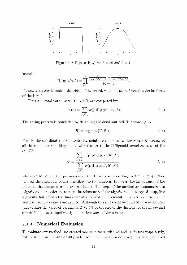
Figure 2.1: Πs

(x; a;b; �) for � = 50 and � = 1.

kernels:

Πs

(x; a;b; �) =

2∏

d=1

11+e−�(x

d

−a

d

) − 11+e−�(x

d

−b

d

)

b

d

− a

d

:

Parameters a and b ontrol the width of the kernel, while the slope � ontrols the fuzziness

of the kernel.

Thus, the total votes asted to ell B

i

are omputed by:

V (Bi

) =∑

p∈Cvp

w(p)Πs

(p; ai

;b

i

; �): (2.2)

The voting pro ess is on luded by dete ting the dominant ell B

∗a ording to:

B

∗ = argmaxB

i

{V (Bi

)}: (2.3)

Finally, the oordinates of the vanishing point are omputed as the weighted average of

all the andidate vanishing points with respe t to the Π-Sigmoid kernel entered at the

ell B

∗:

p

∗ =

∑

p∈Cvp

w(p)pΠs

(p; a∗;b∗; �

∗)

∑

p∈Cvp

w(p)Πs

(p; a∗;b∗; �

∗); (2.4)

where a

∗;b

∗; �

∗are the parameters of the kernel orresponding to B

∗in (2.3). Note

that all the andidate points ontribute to the solution. However, the importan e of the

points in the dominant ell is overwhelming. The steps of the method are summarized in

Algorithm 1. In order to in rease the robustness of the algorithm and to speed it up, line

segments that are shorter than a threshold T and their orientation is lose to horizontal or

verti al within � degrees are pruned. Although this rule ould be omitted, it was dedu ed

that setting the value of parameter T to 5% of the size of the diagonal of the image and

� = ±15o improves signi� antly the performan e of the method.


To evaluate our method, we reated two sequen es, with 35 and 18 frames respe tively,

with a frame size of 320 × 240 pixels ea h. The images in ea h sequen e were aptured

17

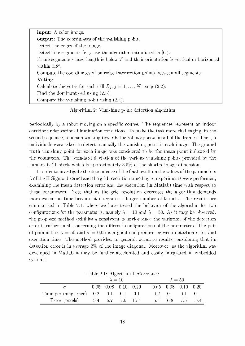
input: A olor image.

output: The oordinates of the vanishing point.

Dete t the edges of the image.

Dete t line segments (e.g. use the algorithm introdu ed in [6℄).

Prune segments whose length is below T and their orientation is verti al or horizontal

within ±�o.Compute the oordinates of pairwise interse tion points between all segments.

Voting

Cal ulate the votes for ea h ell B

j

, j = 1; : : : ; N using (2.2).

Find the dominant ell using (2.3).

Compute the vanishing point using (2.4).

Algorithm 2: Vanishing point dete tion algorithm

periodi ally by a robot moving on a spe i� ourse. The sequen es represent an indoor

orridor under various illumination onditions. To make the task more hallenging, in the

se ond sequen e, a person walking towards the robot appears in all of the frames. Then, 5

individuals were asked to dete t manually the vanishing point in ea h image. The ground

truth vanishing point for ea h image was onsidered to be the mean point indi ated by

the volunteers. The standard deviation of the various vanishing points provided by the

humans is 11 pixels whi h is approximately 3:5% of the shorter image dimension.

In order to investigate the dependen e of the �nal result on the values of the parameters

� of the Π-Sigmoid kernel and the grid resolution tuned by �, experiments were performed,

examining the mean dete tion error and the exe ution (in Matlab) time with respe t to

those parameters. Note that as the grid resolution de reases the algorithm demands

more exe ution time be ause it integrates a larger number of kernels. The results are

summarized in Table 2.1, where we have tested the behavior of the algorithm for two

on�gurations for the parameter �, namely � = 10 and � = 50. As it may be observed,

the proposed method exhibits a onsistent behavior sin e the variation of the dete tion

error is rather small on erning the di�erent on�gurations of the parameters. The pair

of parameters � = 50 and � = 0:05 is a good ompromise between dete tion error and

exe ution time. The method provides, in general, a urate results onsidering that its

dete tion error is in average 2% of the image diagonal. Moreover, as the algorithm was

developed in Matlab it may be further a elerated and easily integrated in embedded

systems.

Table 2.1: Algorithm Performan e

� = 10 � = 50

� 0.05 0.08 0.10 0.20 0.05 0.08 0.10 0.20

Time per image (se ) 0.2 0.1 0.1 0.1 0.2 0.1 0.1 0.1

Error (pixels) 5.4 6.7 7.6 15.4 5.4 6.8 7.5 15.4

18

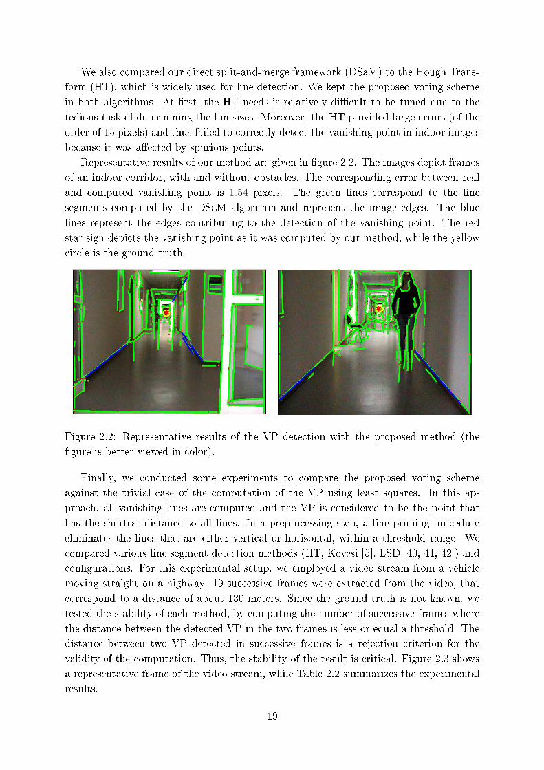
We also ompared our dire t split-and-merge framework (DSaM) to the Hough Trans-

form (HT), whi h is widely used for line dete tion. We kept the proposed voting s heme

in both algorithms. At �rst, the HT needs is relatively diÆ ult to be tuned due to the

tedious task of determining the bin sizes. Moreover, the HT provided large errors (of the

order of 15 pixels) and thus failed to orre tly dete t the vanishing point in indoor images

be ause it was a�e ted by spurious points.

Representative results of our method are given in �gure 2.2. The images depi t frames

of an indoor orridor, with and without obsta les. The orresponding error between real

and omputed vanishing point is 1:54 pixels. The green lines orrespond to the line

segments omputed by the DSaM algorithm and represent the image edges. The blue

lines represent the edges ontributing to the dete tion of the vanishing point. The red

star sign depi ts the vanishing point as it was omputed by our method, while the yellow

ir le is the ground truth.

Figure 2.2: Representative results of the VP dete tion with the proposed method (the

�gure is better viewed in olor).

Finally, we ondu ted some experiments to ompare the proposed voting s heme

against the trivial ase of the omputation of the VP using least squares. In this ap-

proa h, all vanishing lines are omputed and the VP is onsidered to be the point that

has the shortest distan e to all lines. In a prepro essing step, a line pruning pro edure

eliminates the lines that are either verti al or horizontal, within a threshold range. We

ompared various line segment dete tion methods (HT, Kovesi [5℄, LSD [40, 41, 42℄) and

on�gurations. For this experimental setup, we employed a video stream from a vehi le

moving straight on a highway. 19 su essive frames were extra ted from the video, that

orrespond to a distan e of about 130 meters. Sin e the ground truth is not known, we

tested the stability of ea h method, by omputing the number of su essive frames where

the distan e between the dete ted VP in the two frames is less or equal a threshold. The

distan e between two VP dete ted in su essive frames is a reje tion riterion for the

validity of the omputation. Thus, the stability of the result is riti al. Figure 2.3 shows

a representative frame of the video stream, while Table 2.2 summarizes the experimental

results.

19

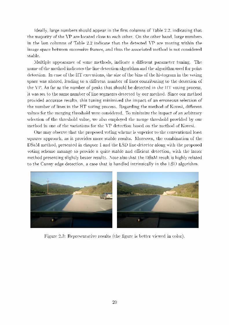
Ideally, large numbers should appear in the �rst olumns of Table 2.2, indi ating that

the majority of the VP are lo ated lose to ea h other. On the other hand, large numbers

in the last olumns of Table 2.2 indi ate that the dete ted VP are moving within the

image spa e between su essive frames, and thus the asso iated method is not onsidered

stable.

Multiple appearan e of some methods, indi ate a di�erent parameter tuning. The

name of the method indi ates the line dete tion algorithm and the algorithm used for point

dete tion. In ase of the HT exe utions, the size of the bins of the histogram in the voting

spa e was altered, leading to a di�erent number of lines ontributing to the dete tion of

the VP. As far as the number of peaks that should be dete ted in the HT voting pro ess,

it was set to the same number of line segments dete ted by our method. Sin e our method

provided a urate results, this tuning minimized the impa t of an erroneous sele tion of

the number of lines in the HT voting pro ess. Regarding the method of Kovesi, di�erent

values for the merging threshold were onsidered. To minimize the impa t of an arbitrary

sele tion of the threshold value, we also employed the merge threshold provided by our

method in one of the variations for the VP dete tion based on the method of Kovesi.

One may observe that the proposed voting s heme is superior to the onventional least

squares approa h, as it provides more stable results. Moreover, the ombination of the

DSaM method, presented in hapter 1 and the LSD line dete tor along with the proposed

voting s heme manage to provide a quite stable and eÆ ient dete tion, with the latter

method presenting slightly better results. Note also that the DSaM result is highly related

to the Canny edge dete tion, a ase that is handled intrinsi ally in the LSD algorithm.

Figure 2.3: Representative results (the �gure is better viewed in olor).

20

Table 2.2: Number of two su essive frames where the distan e of the dete ted VP in the

two frames is less or equal to a threshold

Method

Distan e (in pixels)

1 2 3 4 5 6 7 8 9 10 ≥10

DSaM+Π-Sigmoid 0 0 1 5 6 7 8 9 10 11 8

HT+LSE (1) 0 0 0 0 0 0 0 0 0 0 19

HT+LSE (2) 0 1 1 1 2 2 2 2 3 3 16

HT+LSE (3) 0 0 1 1 1 2 5 5 5 5 14

HT+LSE (4) 0 0 0 0 0 0 0 0 0 0 19

HT+LSE (5) 0 1 1 1 2 2 2 2 3 3 16

Kovesi+Π-Sigmoid (1) 0 0 1 1 1 2 2 2 4 4 15

Kovesi+Π-Sigmoid (2) 0 0 0 0 1 1 1 1 2 3 16

Kovesi+LSE (1) 0 0 0 0 0 0 0 0 0 0 19

Kovesi+LSE (2) 0 0 0 1 1 2 3 4 5 5 14

LSD+Π-Sigmoid 0 0 2 5 7 10 10 10 15 17 2

LSD+LSE 0 0 2 2 2 2 2 4 7 7 12

2.2 Point loud sampling and re onstru tion

2.2.1 Introdu tion

As modern image analysis and omputer vision algorithms have be ome more omplex

requiring a large number of operations and the the data to be pro essed are big, a pre-

pro essing step is a ne essary task that may assist toward eÆ ient and fast pro essing. In

many ases, that step involves sampling an original image or it edge map (e.g. omputa-

tion of the vanishing point) in order to keep a fra tion of points that des ribe with �delity

the initial information. More spe i� ally, in image pro essing, this leads to edge pixel

sampling so as to extra t the eventually hidden patterns (e.g. obje t ontours) inside an

initial observation so that the result is as lose as possible to the observation.

The most straightforward approa h is to apply random sampling, whi h assumes that

the edge points are observations of a random variable that follows a spe i� distribution.

As soon as we model that distribution, point sampling is augmented to sampling obser-

vations from a known distribution. In the simplisti random sampling, it is assumed that

the original set follows a uniform distribution. A more advan ed, but notoriously time

onsuming probabilisti model is Monte Carlo sampling [45℄. J. Malik independently pro-

posed ontour sampling in [57℄ to apply it to an obje t retrieval algorithm [7℄. Initially,

a permutation of the points is omputed and a large number of the samples is drawn

from that permutation. Then iteratively, the pair of points with the minimum pairwise

distan e is dete ted and one of them is kept as a valid sample. This pro ess is iterated

until the desired number of samples is rea hed and it ensures that points from image

regions with large density will be part of the �nal data set.

21

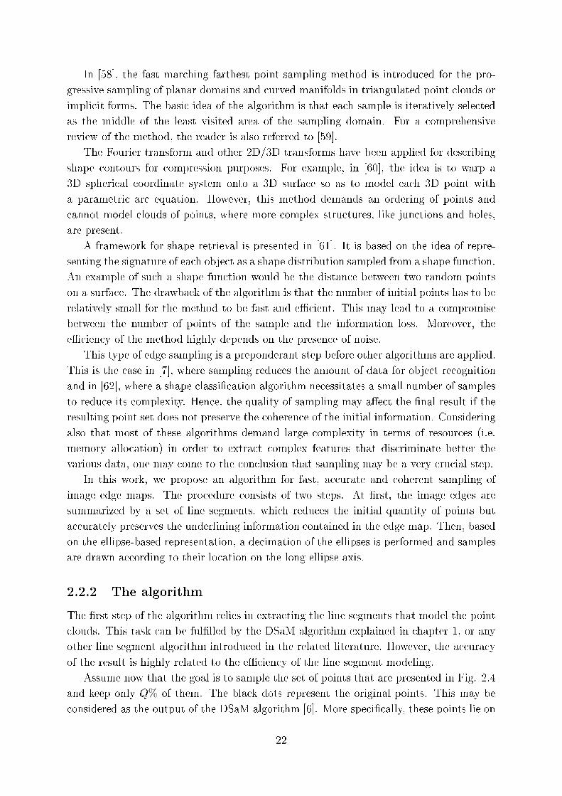
In [58℄, the fast mar hing farthest point sampling method is introdu ed for the pro-

gressive sampling of planar domains and urved manifolds in triangulated point louds or

impli it forms. The basi idea of the algorithm is that ea h sample is iteratively sele ted

as the middle of the least visited area of the sampling domain. For a omprehensive

review of the method, the reader is also referred to [59℄.

The Fourier transform and other 2D/3D transforms have been applied for des ribing

shape ontours for ompression purposes. For example, in [60℄, the idea is to warp a

3D spheri al oordinate system onto a 3D surfa e so as to model ea h 3D point with

a parametri ar equation. However, this method demands an ordering of points and

annot model louds of points, where more omplex stru tures, like jun tions and holes,

are present.

A framework for shape retrieval is presented in [61℄. It is based on the idea of repre-

senting the signature of ea h obje t as a shape distribution sampled from a shape fun tion.

An example of su h a shape fun tion would be the distan e between two random points

on a surfa e. The drawba k of the algorithm is that the number of initial points has to be

relatively small for the method to be fast and eÆ ient. This may lead to a ompromise

between the number of points of the sample and the information loss. Moreover, the

eÆ ien y of the method highly depends on the presen e of noise.

This type of edge sampling is a preponderant step before other algorithms are applied.

This is the ase in [7℄, where sampling redu es the amount of data for obje t re ognition

and in [62℄, where a shape lassi� ation algorithm ne essitates a small number of samples

to redu e its omplexity. Hen e, the quality of sampling may a�e t the �nal result if the

resulting point set does not preserve the oheren e of the initial information. Considering

also that most of these algorithms demand large omplexity in terms of resour es (i.e.

memory allo ation) in order to extra t omplex features that dis riminate better the

various data, one may ome to the on lusion that sampling may be a very ru ial step.

In this work, we propose an algorithm for fast, a urate and oherent sampling of

image edge maps. The pro edure onsists of two steps. At �rst, the image edges are

summarized by a set of line segments, whi h redu es the initial quantity of points but

a urately preserves the underlining information ontained in the edge map. Then, based

on the ellipse-based representation, a de imation of the ellipses is performed and samples

are drawn a ording to their lo ation on the long ellipse axis.

2.2.2 The algorithm

The �rst step of the algorithm relies in extra ting the line segments that model the point

louds. This task an be ful�lled by the DSaM algorithm explained in hapter 1, or any

other line segment algorithm introdu ed in the related literature. However, the a ura y

of the result is highly related to the eÆ ien y of the line segment modeling.

Assume now that the goal is to sample the set of points that are presented in Fig. 2.4

and keep only Q% of them. The bla k dots represent the original points. This may be

onsidered as the output of the DSaM algorithm [6℄. More spe i� ally, these points lie on

22

the long axis of a highly e entri horizontal ellipse. The axis is shown in red. In order

to approximate the lo al point distribution, a histogram is omputed with a number of

bins equal to Q × L, where L is the number of initial points in the set to be sampled.

Then, we represent ea h bin by its mean value, whi h under e.g. Gaussian assumption

it is the geometri enter of the points in the bin and we sele t in ea h bin the point

that is loser (in terms of Eu lidean distan e) to this geometri mean. By repeating the

pro edure for ea h line segment produ ed by the appli ation of the DSaM algorithm we

are able to sample the original point loud.

Figure 2.4: An example of the sampling pro ess. The bla k points represent the original

set of points, while the red line is the is their summary omputed by DSaM [6℄. The

verti al blue lines depi t the limits of the histogram bins. The green points are those

sele ted to represent the sampled set be ause they are loser to the mean value of the bin.

The �gure is better seen in olor.

It may be easily understood that the eÆ ien y of the approa h is highly related to the

orre t determination of a model approximating the lo al manifold of the point set. The

larger the deviation of the model from the lo al manifold be omes, the less a urate is the

sampling method. This is true as the model fails to ompute the histograms orre tly and

therefore to establish a urately the bin enters. Consequently, the sele ted samples will

be less representative of the distribution of the initial edges. For that reason, we relied

on the DSaM algorithm whi h may a urately des ribe the edge map.

An important issue of the sampling algorithm is the value of the sampling frequen y

Q, that is how densely should we sample? Moreover, the number of samples should vary

lo ally with respe t to the number of image edges present in an image region. To this

end, based on the lustering of points to highly e entri ellipses, we propose to sele t

the number of samples to be equal to Æ times the number of points that are present in

the mostly populated ellipse, where Æ ≥ 1:0. This guarantees that, highly on entrated

image regions will be more densely sampled but also that sparse regions should always

have some representatives as they have already been assigned to an ellipse. This is in

ontrast to random or even Monte Carlo based sampling where sparse areas may have no

representatives in the sampled data set.

In other words, the sampling rate is omputed by

Q = Æ

R

L

; (2.5)

where R is the maximum number of members in the lusters, L is the total number of

points in the original set and Æ ≥ 1:0 is a real positive number. The larger the value of

Æ is, the more samples we get, and thus the loser to the initial set our sampling result

is. In other words, the estimation of the p-value of parameter Æ is a ompromise between

the quality of the result and its omplexity.

23

So far we have presented an algorithm for redu ing the number of points in a set with

a minimal impa t regarding the information loss. This rationale, an be extended, to

extra t shapes from point louds. In other words, we will present a method for extra ting

shapes with a desired resolution, in terms of number of points. If we assume that the

manifold lo ally an be approximated linearly, then the DSaM method introdu ed in

se tion 1 an be employeed. A line segment � an be des ribed by its starting and ending

points, x

s

and x

e

respe tively, i.e. � = {xs

;x

e

} where x

s

;x

e

∈ R2. In prin ipal, a line is

modeled by the following equation Ax+By+Γ = 0. where x; y; A; B;Γ ∈ R and (x; y)

is a point laying onto the line. Sin e x

s

and x

e

are given, determining A, B, Γ is trivial.

Then following a similar pro ess with the sampling algorithm des ribed earlier, we an

reprodu e the orresponding shape part, at any desired resolution. Thus, starting from

point x

s

and following the dire tion of the line segment with a prede�ned step � ∈ R+

ea h time, we may re onstru t (approximate) the initial points. The value of the step

� ontrols the density of the result: the higher its value is, the more points we extra t.

Algorithm 3 demonstrates the steps of the proposed shape re onstru tion method.

The ontribution of the DSaM method is that in manages to model a urately enough

the hidden manifold of the point loud and thus provide eÆ ient features (line segments)

for shape re onstru tion. A dire t appli ation of this method would be the eÆ ient

dete tion of the proje tion of random point onto the ontour of a shape, like the method

proposed in [63℄.

input: The set of unordered points X = {xi

|i = 1; : : : ; N}, M ∈ N.

output: The omputed set of points Y = {xi

|i = 1; : : : ;M} that des ribe a shape.

Run the DSaM algorithm (refer to hapter 1) to model the manifold.

Let �

i

= {xis

;x

i

e

}, i = 1; : : : ; K be the line segments extra ted, with x

i

s

; x

i

e

being the

starting and ending points of the i-th segment respe tively.

for i=1:K do

Let Ri

= {ri0; ri2; : : : ; riMi

} be the re onstru ted points based on the segment �

i

, where

r

i

0 = x

i

s

and r

i

M

i

= x

i

e

.

�

i

∈ R = |xie

−xis

|M

i

.

for j=1:M-2 do

r

i

j

= r

i

j−1 + �~e, where ~e is the unit ve tor with dire tion similar to the dire tion of

�

i

.

Y =⋃

K

i=1{Ri

}.

Algorithm 3: Shape re onstru tion from a 2D point loud


For our experiments we used two datasets with ontours of various obje ts: The MPEG7

dataset [1℄ and the Gatorbait dataset [2℄. For more details about those datasets, please

24

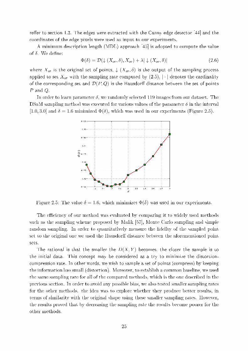
re�er to se tion 1.3. The edges were extra ted with the Canny edge dete tor [44℄ and the

oordinates of the edge pixels were used as input to our experiments.

A minimum des ription length (MDL) approa h [45℄ is adopted to ompute the value

of Æ. We de�ne:

Φ(Æ) = D(↓ (Xor

; Æ); Xor

) + �| ↓ (Xor

; Æ)| (2.6)

where X

or

is the original set of points, ↓ (Xor

; Æ) is the output of the sampling pro ess

applied to set X

or

with the sampling rate omputed by (2.5), | · | denotes the ardinalityof the orresponding set and D(P;Q) is the Hausdor� distan e between the set of points

P and Q.

In order to learn parameter Æ, we randomly sele ted 119 images from our dataset. The

DSaM sampling method was exe uted for various values of the parameter Æ in the interval

[1:0; 3:0] and Æ = 1:6 minimized Φ(Æ), whi h was used in our experiments (Figure 2.5).

Figure 2.5: The value Æ = 1:6, whi h minimizes Φ(Æ) was used in our experiments.

The eÆ ien y of our method was evaluated by omparing it to widely used methods

su h as the sampling s heme proposed by Malik [57℄, Monte Carlo sampling and simple

random sampling. In order to quantitatively measure the �delity of the sampled point

set to the original one we used the Hausdor� distan e between the aforementioned point

sets.

The rational is that the smaller the D(X; Y ) be omes, the loser the sample is to

the initial data. This on ept may be onsidered as a try to minimize the distortion-

ompression rate. In other words, we wish to sample a set of points ( ompress) by keeping

the information loss small (distortion). Moreover, to establish a ommon baseline, we used

the same sampling rate for all of the ompared methods, whi h is the one des ribed in the

previous se tion. In order to avoid any possible bias, we also tested smaller sampling rates

for the other methods. the idea was to explore whether they produ e better results, in

terms of similarity with the original shape using these smaller sampling rates. However,

the results proved that by de reasing the sampling rate the results be ome poorer for the

other methods.

25

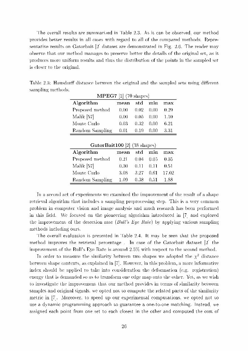
The overall results are summarized in Table 2.3. As it an be observed, our method

provides better results in all ases with regard to all of the ompared methods. Repre-

sentative results on Gatorbait [2℄ dataset are demonstrated in Fig. 2.6. The reader may

observe that our method manages to preserve better the details of the original set, as it

produ es more uniform results and thus the distribution of the points in the sampled set

is loser to the original.

Table 2.3: Hausdor� distan e between the original and the sampled sets using di�erent

sampling methods.


Algorithm mean std min max

Proposed method 0.00 0.02 0.00 0.29

Malik [57℄ 0.00 0.05 0.00 1.10

Monte Carlo 0.03 0.32 0.00 6.21

Random Sampling 0.01 0.19 0.00 3.31


Algorithm mean std min max

Proposed method 0.21 0.04 0.05 0.35

Malik [57℄ 0.30 0.11 0.11 0.51

Monte Carlo 3.08 3.27 0.61 17.02

Random Sampling 1.09 0.38 0.51 1.88

In a se ond set of experiments we examined the improvement of the result of a shape

retrieval algorithm that in ludes a sampling prepro essing step. This is a very ommon

problem in omputer vision and image analysis and mu h resear h has been performed

in this �eld. We fo used on the pioneering algorithm introdu ed in [7℄ and explored

the improvement of the dete tion rate (Bull's Eye Rate) by applying various sampling

methods in luding ours.

The overall evaluation is presented in Table 2.4. It may be seen that the proposed

method improves the retrieval per entage . In ase of the Gatorbait dataset [2℄ the

improvement of the Bull's Eye Rate is around 2:5% with respe t to the se ond method.

In order to measure the similarity between two shapes we adopted the �

2distan e

between shape ontexts, as explained in [7℄. However, in this problem, a more informative

index should be applied to take into onsideration the deformation (e.g. registration)

energy that is demanded so as to transform one edge map onto the other. Yet, as we wish

to investigate the improvement that our method provides in terms of similarity between

samples and original signals, we opted not to ompute the related parts of the similarity

metri in [7℄. Moreover, to speed up our experimental omputations, we opted not to

use a dynami programming approa h to guarantee a one-to-one mat hing. Instead, we

assigned ea h point from one set to ea h losest in the other and omputed the ost of

26

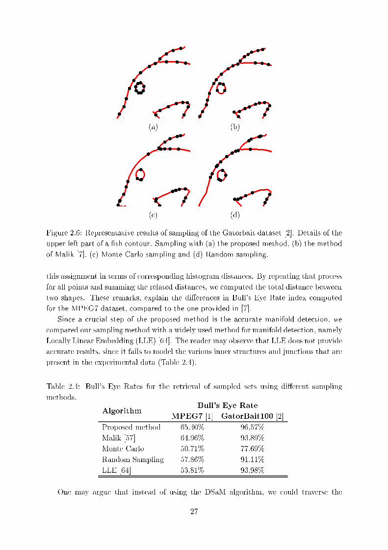
(a) (b)

( ) (d)

Figure 2.6: Representative results of sampling of the Gatorbait dataset [2℄. Details of the

upper left part of a �sh ontour. Sampling with (a) the proposed method, (b) the method

of Malik [7℄, ( ) Monte Carlo sampling and (d) Random sampling.

this assignment in terms of orresponding histogram distan es. By repeating that pro ess

for all points and summing the related distan es, we omputed the total distan e between

two shapes. These remarks, explain the di�eren es in Bull's Eye Rate index omputed

for the MPEG7 dataset, ompared to the one provided in [7℄.

Sin e a ru ial step of the proposed method is the a urate manifold dete tion, we

ompared our sampling method with a widely used method for manifold dete tion, namely

Lo ally Linear Embedding (LLE) [64℄. The reader may observe that LLE does not provide

a urate results, sin e it fails to model the various inner stru tures and jun tions that are

present in the experimental data (Table 2.4).

Table 2.4: Bull's Eye Rates for the retrieval of sampled sets using di�erent sampling

methods.

Algorithm

Bull's Eye Rate

MPEG7 [1℄ GatorBait100 [2℄

Proposed method 65.40% 96.57%

Malik [57℄ 64.96% 93.89%

Monte Carlo 50.71% 77.69%

Random Sampling 57.86% 91.11%

LLE [64℄ 53.81% 93.98%

One may argue that instead of using the DSaM algorithm, we ould traverse the

27

point set by visiting the nearest neighbor of ea h point su essively following a polygon

approximation variation. For demonstration purposes, we all this approa h Nearest-

Neighbor Split (NN-S). Finally, as our algorithm is based on line segment �tting, we also

tested it against one widely used similar algorithm [5℄, that utilizes nearest neighbors.

Moreover, sin e we are dealing with manifold learning from point louds, we also

tested the tensor voting framework, [8, 9℄. Tensor voting is a robust and eÆ ient method,

however its threshold tuning is not trivial and the result is highly related to the sele ted

threshold values. In general, tensor voting, manages to extra t a large part of the ontour.

However, the large distortion is due to the fa t that some parts of the shape silhouette

are missing, i.e. holes are present, or new points are added, that are not present in the

pure data. For our experiments, we sele ted those threshold values that provided the

best result. Figure 2.7 demonstrates the results of our experiments. As it an be seen in

the �gures, the proposed method provides more a urate results ompared to the other

methods in terms of shape re onstru tion as it is explained below.

For this experimental on�guration, we disturbed the shape silhouettes with additive

Gaussian noise with progressively in reasing varian e. The evaluation of the method is

based on a distortion- ompression model for varying signal-to-noise (SNR) ratio, where

the distortion is measured in terms of shape similarity between the re onstru ted shape

and the initial one, and ompression is the number of segments omputed via DSaM over

the total number of points. Please note that although this approa h is similar to our

analysis in 1, in this se tion the distortion is omputed in a di�erent way, whi h is more

meaningful in the ontext of the appli ation.

28

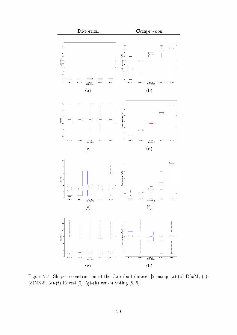
Distortion Compression

(a) (b)

( ) (d)

(e) (f)

(g) (h)

Figure 2.7: Shape re onstru tion of the Gatorbait dataset [2℄ using (a)-(b) DSaM, ( )-

(d)NN-S, (e)-(f) Kovesi [5℄, (g)-(h) vensor voting [8, 9℄.

29

2.3 Shape en oding for edge map image ompression

2.3.1 Introdu tion

Shape representation is a signi� ant task in image storage and transmission, as it an

be used to represent obje ts at a lower omputational ost, ompared to non-en oded

representations. For example, the widely used MPEG4 Part 2 obje t-based video standard

uses shape oding for des ribing regions, alled video obje t planes, that represent an

obje t [65℄. In that ase, a urate shape en oding leads to better preservation of ontour

details.

The pioneering work in [66℄, where sequen es of line segments of spe i�ed length and

dire tion are represented by hain odes was proposed for the des ription of digitized

urves, ontours and drawings and it was followed by numerous te hniques. Shape oding

is a �eld that has been studied extensively in the past but it is still very a tive. Vari-

ous methods have been studied in [67℄, in luding the ontext-based arithmeti en oding

(CAE), whi h has been adopted by the MPEG4 Part 2 standard.

The digital straight line segments oder (DSLSC) was introdu ed in [68℄ for oding

bilevel images with lo ally straight edges, that is, single binary shape images and bilevel

layers of digital maps. DSLS models the edges by digital straight line segments (DSLS)

[69℄. Compared to standard algorithms like JBIG [70℄, JBIG-2 [71℄ and MPEG4 CAE

[65℄,[67℄ DSLSC provides better results, as it fully exploits the information given by the

lo al straightness of the boundary, whi h is not hte ase for the other methods.

DSLSC is further improved in [72℄, where the segmentation of the alpha plane in three

layers (binary shape layer, opaque layer, and intermediate layer) is employed. Experimen-

tal results demonstrated substantial bit rate savings for oding shape and transparen y

when ompared to the tools adopted in MPEG4 Part 2.

Dis rete straight lines were also employed in [73℄ for shape en oding and improvement

of the ompression rate is rea hed by arrying out a pattern substrings analysis to �nd

high redundan y in binary shapes.

A lossless ompression of map ontours by ontext tree modeling of hain odes is

des ribed in [74℄. An optimal n-ary in omplete ontext tree is proposed to be used for

improving the ompression rate.

A JBIG-based approa h for en oding ontour shapes is introdu ed in [75℄, where a

method is presented that manages to eÆ iently ode maps of transition points, outper-

forming, in most ases, di�erential hain- oding.

2.3.2 The algorithm

Line segments are important features in omputer vision, as they an en ode ri h infor-

mation with low omplexity. We take advantage of this feature for en oding a 2D set of

points des ribing a shape as a olle tion of line segments that approximate the manifold

of the shape, by assuming that the manifold is lo ally linear. The initial and ending

points of ea h line segment may be onsidered as the hara teristi points arrying the

30

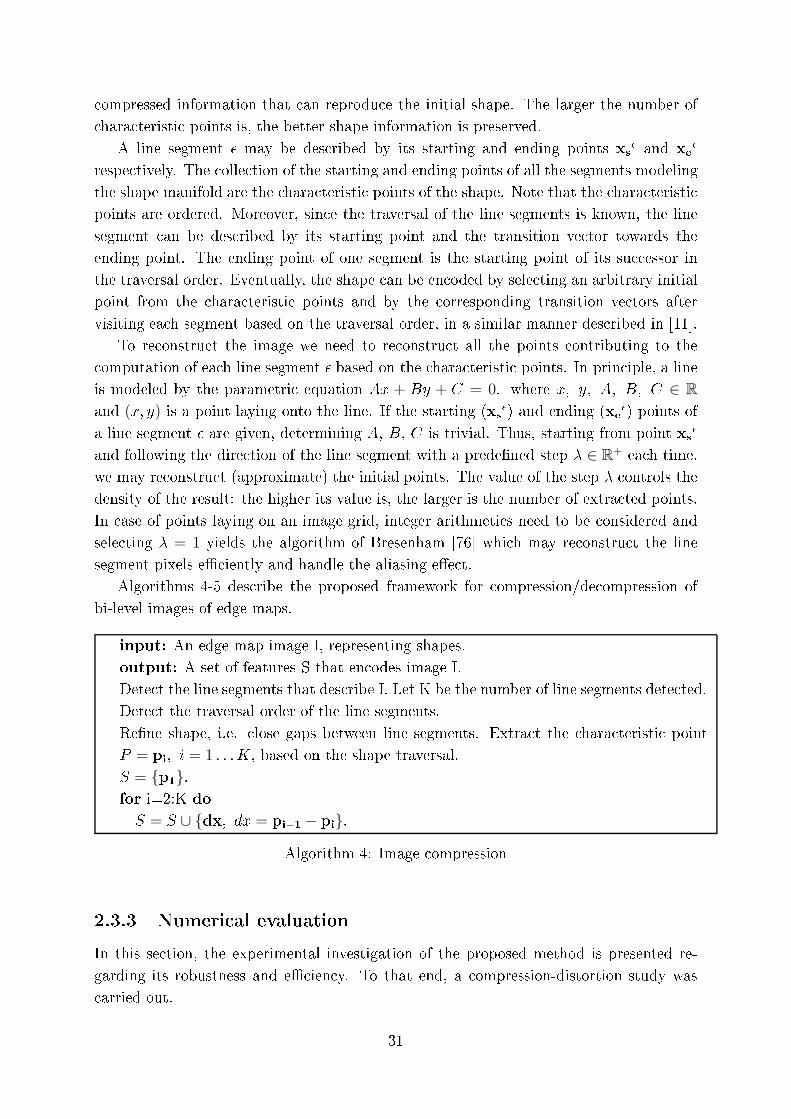
ompressed information that an reprodu e the initial shape. The larger the number of

hara teristi points is, the better shape information is preserved.

A line segment � may be des ribed by its starting and ending points x

s

�

and x

e

�

respe tively. The olle tion of the starting and ending points of all the segments modeling

the shape manifold are the hara teristi points of the shape. Note that the hara teristi

points are ordered. Moreover, sin e the traversal of the line segments is known, the line

segment an be des ribed by its starting point and the transition ve tor towards the

ending point. The ending point of one segment is the starting point of its su essor in

the traversal order. Eventually, the shape an be en oded by sele ting an arbitrary initial

point from the hara teristi points and by the orresponding transition ve tors after

visiting ea h segment based on the traversal order, in a similar manner des ribed in [11℄.

To re onstru t the image we need to re onstru t all the points ontributing to the

omputation of ea h line segment � based on the hara teristi points. In prin iple, a line

is modeled by the parametri equation Ax + By + C = 0. where x; y; A; B; C ∈ R

and (x; y) is a point laying onto the line. If the starting (x

s

�

) and ending (x

e

�

) points of

a line segment � are given, determining A, B, C is trivial. Thus, starting from point x

s

�

and following the dire tion of the line segment with a prede�ned step � ∈ R+ea h time,

we may re onstru t (approximate) the initial points. The value of the step � ontrols the

density of the result: the higher its value is, the larger is the number of extra ted points.

In ase of points laying on an image grid, integer arithmeti s need to be onsidered and

sele ting � = 1 yields the algorithm of Bresenham [76℄ whi h may re onstru t the line

segment pixels eÆ iently and handle the aliasing e�e t.

Algorithms 4-5 des ribe the proposed framework for ompression/de ompression of

bi-level images of edge maps.

input: An edge map image I, representing shapes.

output: A set of features S that en odes image I.

Dete t the line segments that des ribe I. Let K be the number of line segments dete ted.

Dete t the traversal order of the line segments.

Re�ne shape, i.e. lose gaps between line segments. Extra t the hara teristi point

P = p

i

; i = 1 : : :K, based on the shape traversal.

S = {p1

}.for i=2:K do

S = S ∪ {dx; dx = p

i−1 − p

i

}.

Algorithm 4: Image ompression


In this se tion, the experimental investigation of the proposed method is presented re-

garding its robustness and eÆ ien y. To that end, a ompression-distortion study was

arried out.

31

input: A set of features S that en odes an image I.

output: The re onstru ted image I.

Re over the hara teristi points P = {pi

; i = 1 : : :K}, based on initial point and

transitions en oded in S.

for i=2:K do

Produ e the set of points R, e.g. [76℄, ontaining the points of the line segment from

p

i−1 to pi.

Set the pixels of I orresponding to oordinates of points in R on.

Algorithm 5: Image de ompression

Compression was omputed as the ratio of the �le size between the ompressed and

the original �les. Various lossless methods were onsidered and the orresponding size of

the output �les they produ ed was used as the referen e original �le size. The methods

against whi h we ompared the proposed framework are the CCITT G4 standard [77℄

(denoted as FAX4 herein), adopted amongst others by the TIFF image �le format for

binary images, and the widely used standards JBIG [70℄ and JBIG2 [71℄.

As far as the distortion is on erned, a twofold omputation was performed in terms

of measuring the loss of information and the similarity between the initial and the �nal

edge map images. Therefore, the distortion index adopted by MPEG4 [78℄, given by

D

R

=Number of pixels in error

Number of interior pixels

; (2.7)

was also used in this work. The Hausdor� distan e between the original edge map X and

the re onstru ted edge map Y s, given by

D

H

(X; Y ) = maxx∈X

miny∈Y

{|x− y|1}; (2.8)

was used to measure the similarity between X and Y .

For the experimental study, we used two datasets. The Gatorbait dataset [2℄ ontains

the silhouettes of 38 �shes, belonging to 8 ategories. The MPEG7 dataset [1℄ ontains

1400 obje t ontours belonging to 70 ategories, with 20 members per ea h ategory. All

datasets onsist of binary images. In the ase of the Gatorbait100 dataset, the images

were initially thinned so as to extra t the ontour line. Let us note that in this ase, there

are some inner stru tures that were also onsidered in our experiments.

The overall results of our experimental analysis are demonstrated in Tables 2.5 and

2.6, with results for various on�gurations of the line segment dete tion algorithms onsid-

ered. The values next to the method pre�x in the �rst olumn of the Tables indi ates the

orresponding on�guration of the method. We used the line segment method presented

in hapter 1 and the widely used polygon approximation [10℄, as proposed in [11℄. In our

study the values onsidered for the DSaM thresholds were {[0:3; 2:0]; [0:4; 2:0]; [0:5; 2:0]; [0:8; 2:0];[1:3; 2:0]; [2:3; 2:0]}. The se ond threshold was measured in pixels. As far as the poly-

gon approximation (PA) is on erned, this algorithm applies one threshold ontrolling

32

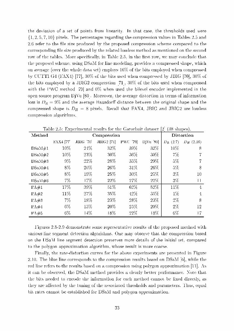
the deviation of a set of points from linearity. In that ase, the thresholds used were

{1; 2; 5; 7; 10} pixels. The per entages regarding the ompression values in Tables 2.5 and

2.6 refer to the �le size produ ed by the proposed ompression s heme ompared to the

orresponding �le size produ ed by the related lossless method as mentioned on the se ond

row of the tables. More spe i� ally, in Table 2.5, in the �rst row, we may on lude that

the proposed s heme, using DSaM for line modeling, provides a ompressed shape, whi h

on average (over the whole data set) employs 16% of the bits employed when ompressed

by CCTTI G4 (FAX4) [77℄, 30% of the bits used when ompressed by JBIG [70℄, 30% of

the bits employed by a JBIG2 ompression [71℄, 30% of the bits used when ompressed

with the PWC method [79℄ and 0% when used the bilevel en oder implemented in the

open sour e program DjVu [80℄. Moreover, the average distortion in terms of information

loss is D

R

= 9% and the average Hausdor� distan e between the original shape and the

ompressed shape is D

H

= 8 pixels. Re all that FAX4, JBIG and JBIG2 are lossless

ompression algorithms.

Table 2.5: Experimental results for the Gatorbait dataset [2℄ (38 shapes).

Method Compression Distortion

FAX4 [77℄ JBIG [70℄ JBIG2 [71℄ PWC [79℄ DjVu [80℄ D

R

(2.7) D

H

(2.16)

DSaM#1 10% 24% 32% 39% 32% 10% 8

DSaM#2 10% 23% 30% 36% 30% 7% 7

DSaM#3 9% 22% 28% 35% 29% 5% 7

DSaM#4 8% 20% 26% 31% 26% 5% 8

DSaM#5 8% 19% 25% 30% 25% 3% 10

DSaM#6 7% 17% 22% 27% 22% 3% 11

PA#1 17% 39% 51% 62% 52% 11% 4

PA#2 11% 27% 35% 42% 35% 1% 4

PA#3 7% 18% 23% 28% 23% 2% 8

PA#4 6% 15% 20% 25% 20% 2% 12

PA#5 6% 14% 18% 22% 18% 6% 17

Figures 2.8-2.9 demonstrate some representative results of the proposed method with

various line segment dete tion algorithms. One may observe that the ompression based

on the DSaM line segment dete tion preserves more details of the initial set, ompared

to the polygon approximation algorithm, whose result is more oarse.

Finally, the rate-distortion urves for the above experiments are presented in Figure

2.10. The blue line orresponds to the ompression results based on DSaM [6℄, while the

red line refers to the results based on a ompression using polygon approximation [11℄. As

it an be observed, the DSaM method provides a learly better performan e. Note that

the bits needed to en ode the information for ea h method annot be �xed dire tly, as

they are a�e ted by the tuning of the asso iated thresholds and parameters. Thus, equal

bit rates annot be established for DSaM and polygon approximation.

33

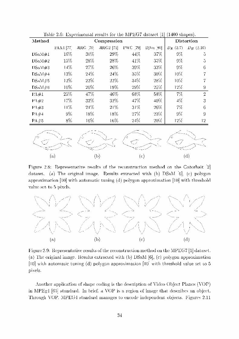
Table 2.6: Experimental results for the MPEG7 dataset [1℄ (1400 shapes).



R

(2.7) D

H

(2.16)

DSaM#1 16% 30% 29% 44% 37% 9% 5

DSaM#2 15% 28% 28% 41% 35% 9% 5

DSaM#3 14% 27% 26% 39% 33% 9% 6

DSaM#4 13% 24% 24% 35% 30% 10% 7

DSaM#5 12% 23% 22% 34% 28% 10% 7

DSaM#6 10% 20% 19% 29% 25% 12% 9

PA#1 25% 47% 46% 68% 58% 7% 2

PA#2 17% 32% 32% 47% 40% 4% 3

PA#3 11% 21% 21% 31% 26% 7% 6

PA#4 9% 18% 18% 27% 23% 9% 9

PA#5 8% 16% 16% 24% 20% 12% 12

(a) (b) ( ) (d)

Figure 2.8: Representative results of the re onstru tion method on the Gatorbait [2℄

dataset. (a) The original image. Results extra ted with (b) DSaM [6℄, ( ) polygon

approximation [10℄ with automati tuning (d) polygon approximation [10℄ with threshold

value set to 5 pixels.

(a) (b) ( ) (d)

Figure 2.9: Representative results of the re onstru tion method on the MPEG7 [1℄ dataset.

(a) The original image. Results extra ted with (b) DSaM [6℄, ( ) polygon approximation

[10℄ with automati tuning (d) polygon approximation [10℄ with threshold value set to 5

pixels.

Another appli ation of shape oding is the des ription of Video Obje t Planes (VOP)

in MPEg4 [65℄ standard. In brief, a VOP is a region of image that des ribes an obje t.

Through VOP, MPEG4 standard manages to en ode independent obje ts. Figures 2.11

34

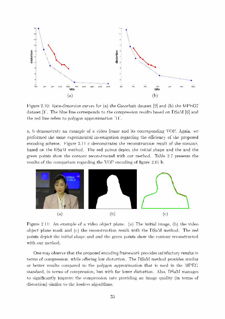
(a) (b)

Figure 2.10: Rate-distortion urves for (a) the Gatorbait dataset [2℄ and (b) the MPEG7

dataset [1℄. The blue line orresponds to the ompression results based on DSaM [6℄ and

the red line refers to polygon approximation [11℄.

a, b demonstrate an example of a video frame and its orresponding VOP. Again, we

performed the same experimental investigation regarding the eÆ ien y of the proposed

en oding s heme. Figure 2.11 demonstrates the re onstru tion result of the ontour,

based on the DSaM method. The red points depi t the initial shape and the and the

green points show the ontour re onstru ted with our method. Table 2.7 presents the

results of the omparison regarding the VOP en oding of �gure 2.11 b.

(a) (b) ( )

Figure 2.11: An example of a video obje t plane. (a) The initial image, (b) the video

obje t plane mask and ( ) the re onstru tion result with the DSaM method. The red

points depi t the initial shape and and the green points show the ontour re onstru ted

with our method.

One may observe that the proposed en oding framework provides satisfa tory results in

terms of ompression, while o�ering low distortion. The DSaM method provides similar

or better results ompared to the polygon approximation that is used in the MPEG

standard, in terms of ompression, but with far lower distortion. Also, DSaM manages

to signi� antly improve the ompression rate providing an image quality (in terms of

distortion) similar to the lossless algorithms.

35

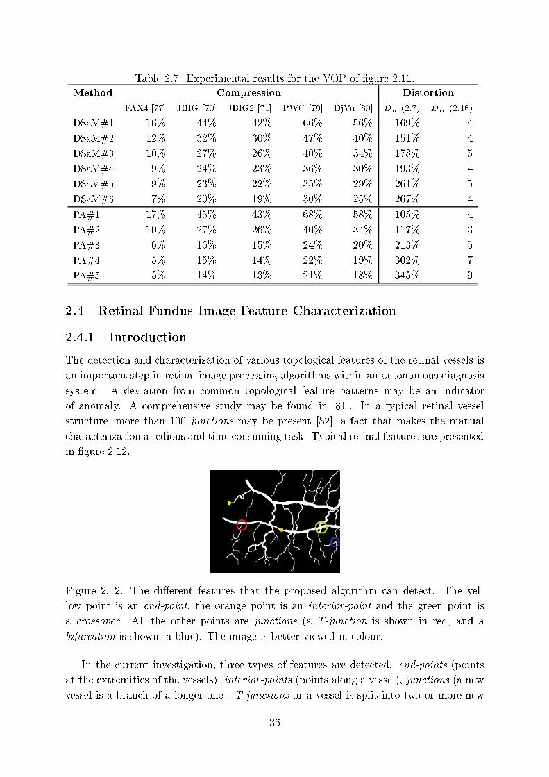
Table 2.7: Experimental results for the VOP of �gure 2.11.



R

(2.7) D

H

(2.16)

DSaM#1 16% 44% 42% 66% 56% 169% 4

DSaM#2 12% 32% 30% 47% 40% 151% 4

DSaM#3 10% 27% 26% 40% 34% 178% 5

DSaM#4 9% 24% 23% 36% 30% 193% 4

DSaM#5 9% 23% 22% 35% 29% 261% 5

DSaM#6 7% 20% 19% 30% 25% 267% 4

PA#1 17% 45% 43% 68% 58% 105% 4

PA#2 10% 27% 26% 40% 34% 117% 3

PA#3 6% 16% 15% 24% 20% 213% 5

PA#4 5% 15% 14% 22% 19% 302% 7

PA#5 5% 14% 13% 21% 18% 345% 9

2.4 Retinal Fundus Image Feature Chara terization

2.4.1 Introdu tion

The dete tion and hara terization of various topologi al features of the retinal vessels is

an important step in retinal image pro essing algorithms within an autonomous diagnosis

system. A deviation from ommon topologi al feature patterns may be an indi ator

of anomaly. A omprehensive study may be found in [81℄. In a typi al retinal vessel

stru ture, more than 100 jun tions may be present [82℄, a fa t that makes the manual

hara terization a tedious and time onsuming task. Typi al retinal features are presented

in �gure 2.12.

Figure 2.12: The di�erent features that the proposed algorithm an dete t. The yel-

low point is an end-point, the orange point is an interior-point and the green point is

a rossover. All the other points are jun tions (a T-jun tion is shown in red, and a

bifur ation is shown in blue). The image is better viewed in olour.

In the urrent investigation, three types of features are dete ted: end-points (points

at the extremities of the vessels), interior-points (points along a vessel), jun tions (a new

vessel is a bran h of a longer one - T-jun tions or a vessel is split into two or more new

36

vessels - bifur ation) and rossovers (one vessel passes over another). Please note that

further pro essing is needed to distinguish between a rossover and a bifur ation.

A methodology that extra ts features from the retinal fundus image and hara terizes

them will be presented. The goal is to dete t the interse tion points between the vessels,

as they ould provide useful information to an automati diagnosis system.

2.4.2 The algorithm

The �rst step of our method is to extra t the line segments that model the enter line of

the vessels. Thus, it is ru ial that an a urate prepro essing step towards that dire tion

is applied. For ea h line segment, its extreme points are the points that have the largest

distan e from the orresponding extreme points of the same line luster.

In �gure 2.13, the points x (summarizing the vessel stru ture) are depi ted with red

and bla k olor, while the orresponding extreme points y are presented with green and

blue dots. A rule is de�ned to hara terize a point as end point or jun tion or rossover.

Let C(x) be the index of the line luster point where x belongs to. In �gure 2.13, two

line lusters are shown (C(x) = 1 and C(x) = 2). To de�ne the neighborhood of extreme

points, a neighborhood radius threshold is de�ned as

T

n

= w ∗ d (2.9)

where d is the mean distan e between all the nearest neighbors and w is a onstant that is

learned, as explained later in this se tion. Thus, for an extreme point y the neighborhood

N (y) is the set of the points x su h that ||x−y|| ≤ T

n

. Note that y ∈ N (y). In order to

hara terize point y, we de�ne CN (y) as the number of distin t line lusters that points

x ∈ N (y) belong to.

In the example shown in �gure 2.13, the studied extreme point y is the green one,

while its neighborhood N (y) is de�ned by a ir le entered at y with radius T

n

. Red and

bla k points lying within that ir le are the neighbors of y. Those points belong either

to line luster 1 or to line luster 2 and thus CN (y) = 2. If all neighbors of y belong to

the same line luster with that of y, then y would be an end-point (CN (y) = 1). In ase

where CN (y) > 2, y would be a jun tion or a rossover. The algorithm in its urrent

form does not dis riminate between them.

A spe ial ase o urs when CN (y) = 2, where the studied point y is either an interior-

point or a jun tion (T-jun tion). In that ase, further elaboration is needed to hara terize

the extreme point by examining whether N (y) ontains an extreme point or not. Thus, if

y belongs also to the neighborhood of y

′, with y

′denoting the neighbor of y, then y is an

interior-point, otherwise it is a jun tion (T-jun tion). Please note that the neighboring

relationship we are des ribing in that se tion is not re e tive. For example in �gure 2.13,

the green point, whi h is one of the extreme points of luster 1, is neighbor to luster 2 (as

there are some points of luster 2 within the yellow ir le that de�nes the neighborhood

of the green point). However, none of the extreme points of luster 2 ontain a point from

luster 1 in their neighborhood, and thus luster 1 is not neighboring to luster 2.

37

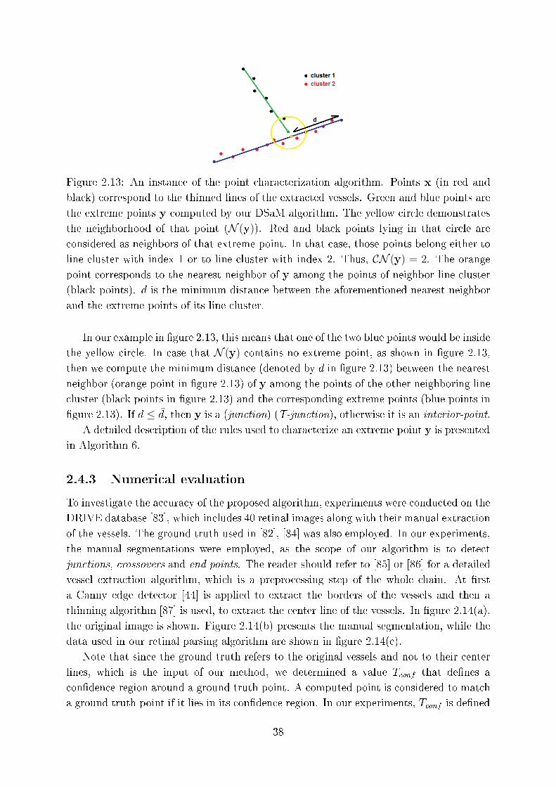
Figure 2.13: An instan e of the point hara terization algorithm. Points x (in red and

bla k) orrespond to the thinned lines of the extra ted vessels. Green and blue points are

the extreme points y omputed by our DSaM algorithm. The yellow ir le demonstrates

the neighborhood of that point (N (y)). Red and bla k points lying in that ir le are

onsidered as neighbors of that extreme point. In that ase, those points belong either to

line luster with index 1 or to line luster with index 2. Thus, CN (y) = 2. The orange

point orresponds to the nearest neighbor of y among the points of neighbor line luster

(bla k points). d is the minimum distan e between the aforementioned nearest neighbor

and the extreme points of its line luster.

In our example in �gure 2.13, this means that one of the two blue points would be inside

the yellow ir le. In ase that N (y) ontains no extreme point, as shown in �gure 2.13,

then we ompute the minimum distan e (denoted by d in �gure 2.13) between the nearest

neighbor (orange point in �gure 2.13) of y among the points of the other neighboring line

luster (bla k points in �gure 2.13) and the orresponding extreme points (blue points in

�gure 2.13). If d ≤ d, then y is a (jun tion) (T-jun tion), otherwise it is an interior-point.

A detailed des ription of the rules used to hara terize an extreme point y is presented

in Algorithm 6.


To investigate the a ura y of the proposed algorithm, experiments were ondu ted on the

DRIVE database [83℄, whi h in ludes 40 retinal images along with their manual extra tion

of the vessels. The ground truth used in [82℄, [84℄ was also employed. In our experiments,

the manual segmentations were employed, as the s ope of our algorithm is to dete t

jun tions, rossovers and end points. The reader should refer to [85℄ or [86℄ for a detailed

vessel extra tion algorithm, whi h is a prepro essing step of the whole hain. At �rst

a Canny edge dete tor [44℄ is applied to extra t the borders of the vessels and then a

thinning algorithm [87℄ is used, to extra t the enter line of the vessels. In �gure 2.14(a),

the original image is shown. Figure 2.14(b) presents the manual segmentation, while the

data used in our retinal parsing algorithm are shown in �gure 2.14( ).

Note that sin e the ground truth refers to the original vessels and not to their enter

lines, whi h is the input of our method, we determined a value T

onf

that de�nes a

on�den e region around a ground truth point. A omputed point is onsidered to mat h

a ground truth point if it lies in its on�den e region. In our experiments, T

onf

is de�ned

38

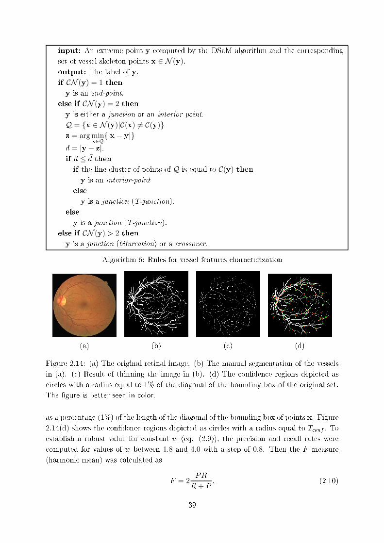
input: An extreme point y omputed by the DSaM algorithm and the orresponding

set of vessel skeleton points x ∈ N (y).

output: The label of y.

if CN (y) = 1 then

y is an end-point.

else if CN (y) = 2 then

y is either a jun tion or an interior-point.

Q = {x ∈ N (y)|C(x) 6= C(y)}z = argmin

x∈Q{|x− y|}

d = |y − z|.if d ≤ d then

if the line luster of points of Q is equal to C(y) theny is an interior-point

else

y is a jun tion (T-jun tion).

else

y is a jun tion (T-jun tion).

else if CN (y) > 2 then

y is a jun tion (bifur ation) or a rossover.

Algorithm 6: Rules for vessel features hara terization

(a) (b) ( ) (d)

Figure 2.14: (a) The original retinal image. (b) The manual segmentation of the vessels

in (a). ( ) Result of thinning the image in (b). (d) The on�den e regions depi ted as

ir les with a radius equal to 1% of the diagonal of the bounding box of the original set.

The �gure is better seen in olor.

as a per entage (1%) of the length of the diagonal of the bounding box of points x. Figure

2.14(d) shows the on�den e regions depi ted as ir les with a radius equal to T

onf

. To

establish a robust value for onstant w (eq. (2.9)), the pre ision and re all rates were

omputed for values of w between 1:8 and 4:0 with a step of 0:8. Then the F measure

(harmoni mean) was al ulated as

F = 2PR

R+ P

; (2.10)

39

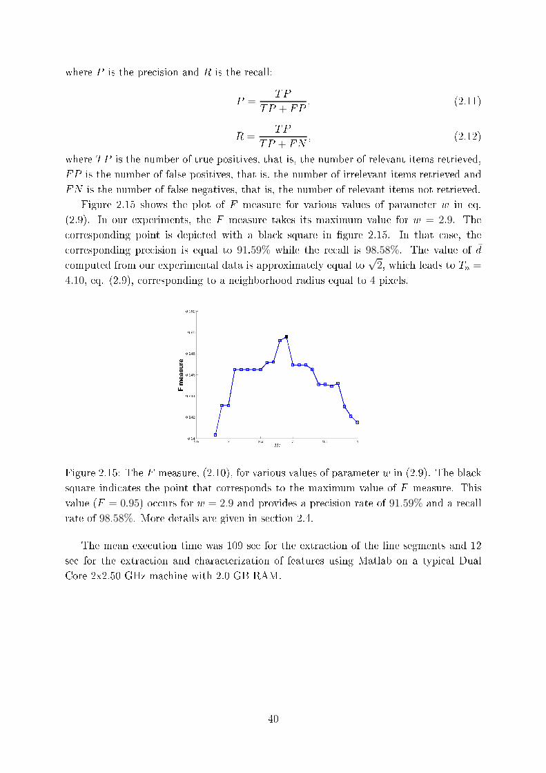
where P is the pre ision and R is the re all:

P =TP

TP + FP

; (2.11)

R =TP

TP + FN

; (2.12)

where TP is the number of true positives, that is, the number of relevant items retrieved,

FP is the number of false positives, that is, the number of irrelevant items retrieved and

FN is the number of false negatives, that is, the number of relevant items not retrieved.

Figure 2.15 shows the plot of F measure for various values of parameter w in eq.

(2.9). In our experiments, the F measure takes its maximum value for w = 2:9. The

orresponding point is depi ted with a bla k square in �gure 2.15. In that ase, the

orresponding pre ision is equal to 91:59% while the re all is 98:58%. The value of d

omputed from our experimental data is approximately equal to

√2, whi h leads to T

n

=

4:10, eq. (2.9), orresponding to a neighborhood radius equal to 4 pixels.

Figure 2.15: The F measure, (2.10), for various values of parameter w in (2.9). The bla k

square indi ates the point that orresponds to the maximum value of F measure. This

value (F = 0:95) o urs for w = 2:9 and provides a pre ision rate of 91:59% and a re all

rate of 98:58%. More details are given in se tion 2.4.

The mean exe ution time was 109 se for the extra tion of the line segments and 12

se for the extra tion and hara terization of features using Matlab on a typi al Dual

Core 2x2.50 GHz ma hine with 2.0 GB RAM.

40

2.5 Elimination of outliers from 2D point sets using the Helmholtz

prin iple

2.5.1 Introdu tion

The modeling and removal of outliers from a set of points has been an a tive resear h topi

for many de ades in image pro essing and omputer vision and a variety of algorithms

have been proposed [88℄. They may be as simple as the median �lter to more elaborate

whi h are based on random sampling, like RANSAC [36℄ or probabilisti models [89℄.

The Gaussian assumption for data generation has been widely adopted but it is ap-

propriate only for sparse outlier distributions. In general, it involves the omparison of

Eu lidean distan es between points with the mean of the distribution expanded by a

number of standard deviation [90℄. Kernel density estimators-based methods provide a

probabilisti approa h to determine if a point belongs to the un orrupted set and are

inherently related to lustering or lassi� ation te hniques that separate pure data from

outliers [91, 92℄.

The number of neighbors of a point is a key issue in hara terizing it as outlier [93℄. The

main hypothesis is that pure data are more densely populated than outlying points and

many algorithms have been designed based on this idea. The adopted strategy onsists

in de�ning a neighborhood for ea h point, determining a feature that hara terizes the

neighborhood and reje ting points with features having a value smaller than a threshold.

In [12℄, the number of ommon neighbors is de�ned as a similarity index between points

and points with neighborhood size smaller than a threshold are reje ted as outliers. An

o tree is used in [94℄ to luster points and an impli it quadri is �t to them to smooth

out outliers.

Inspired by the geometri Gestalt theory, whi h addresses the answer to the funda-

mental problem in omputer vision: "How to arrive at global per epts from the lo al,

atomi information ontained in an image?" [95℄, Desolneux et al. proposed methods for

dete ting geometri stru tures [39℄ and edges [96℄ in images by a parameter free method

based on the Helmholtz prin iple [97℄. The prin iple states that an observed geometri

stru ture is per eptually meaningful if its number of o urren es is very small in a random

situation. In this ontext, geometri stru tures are hara terized as large deviations from

randomness. The prin iple is a ompanied by an a ontrario assumption against whi h

stru tures are dete ted.

In this se tion, we propose an algorithm for outlier elimination and stru ture extra tion

from 2D point louds based on the Helmholtz prin iple. The main di�eren e with the

methods in [39, 96℄ is that the input to the algorithm is not an image whose pixels lay on a

regular grid but a set of s attered points irregularly distributed in spa e. To over ome this

limitation, at �rst, the point set is approximated by a lo ally linear manifold onsisting

of a set of line segments. We show that the lengths of the line segments follow a Pareto

distribution whi h is our a ontrario model.

41

2.5.2 The Helmholtz prin iple

The Helmholtz prin iple is a general hypothesis of the Gestalt theory [95℄ interpreting the

way human per eption works. Intuitively, it states that if we take into onsideration ran-

domness as the normal ase for our observations then meaningful features and interesting

events should not be expe ted. Consequently, if they are observed they should appear

with a small probability. Moreover, the small probability of observing an event is not a

fa tor to onsider it as meaningful (or true observation not generated by noise). Take

as an example the toss of an unbiased oin. The probability of getting a head (H) or a

tail (T ) is 1=2 respe tively. If we toss the oin su essively N times then the probability

of observing any of the possible sequen es of H and T is (1=2)N , whi h is a de reasing

fun tion of N and approa hes zero as N → ∞. More spe i� ally, the following sequen es:

S1 = HTHHTTTHTHHTHT:::H

︸︷︷︸

N times

S2 = HHHHHHHHHHHHH:::H

︸︷︷︸

N times

have equal probabilities of appearan e. However, S2 is not expe ted to appear for an

unbiased oin. Therefore, the low probability of an event may not hara terize it as a

deviation from randomness, as its probability may not truly model the randomness of an

event.

Using the same sequen es S1 and S2, we may de�ne another pair of random variables

n

H

and n

T

modeling the number of H and T present in a sequen e. Sin e the oin is

unbiased, the expe tations of both variables is N=2. Although this is on�rmed in S1,

in sequen e S2 the observed values for n

H

and n

T

is N and 0 largely deviating from the

expe ted values.

The above observations lead to the on lusion that the small probability of an event

may not be an a urate indi ation that this event is meaningful and we need to take into

onsideration that the model we use to validate an event des ribes the randomness of

all possible observations. Turning ba k to the last example of the oin toss, randomness

was modeled only by ounting the number of H and T in a sequen e and not by the

probability of a sequen e to appear. Taking both issues into a ount yields the omplete

model used to des ribe randomness whi h is alled a ontrario model.

2.5.3 The algorithm

LetX = {xi

}i=1;:::;N be a set of observed 2D points in luding both data points and outliers

(Fig. 2.16(a)).

In order to eliminate the outliers, we ompute at �rst an approximation of the point

set by line segments. To this end, the dire t split-and-merge (DSaM) algorithm presented

in hapter 1 an be employed, whi h summarizes any point set by a set of the major axes

of highly e entri ellipses. The number of ellipses is automati ally determined by the

42

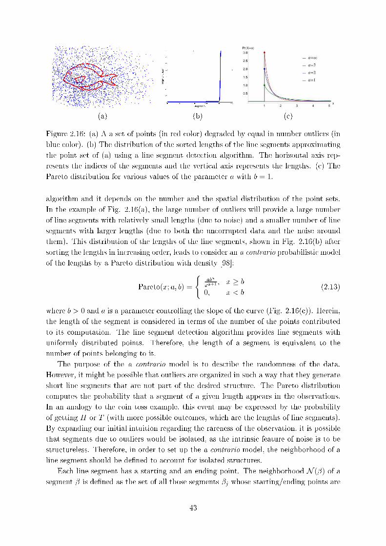
(a) (b) ( )

Figure 2.16: (a) A a set of points (in red olor) degraded by equal in number outliers (in

blue olor). (b) The distribution of the sorted lengths of the line segments approximating

the point set of (a) using a line segment dete tion algorithm. The horizontal axis rep-

resents the indi es of the segments and the verti al axis represents the lengths. ( ) The

Pareto distribution for various values of the parameter a with b = 1.

algorithm and it depends on the number and the spatial distribution of the point sets.

In the example of Fig. 2.16(a), the large number of outliers will provide a large number

of line segments with relatively small lengths (due to noise) and a smaller number of line

segments with larger lengths (due to both the un orrupted data and the noise around

them). This distribution of the lengths of the line segments, shown in Fig. 2.16(b) after

sorting the lengths in in reasing order, leads to onsider an a ontrario probabilisti model

of the lengths by a Pareto distribution with density [98℄:

Pareto(x; a; b) =

{ab

a

x

a+1 ; x ≥ b

0; x < b

(2.13)

where b > 0 and a is a parameter ontrolling the slope of the urve (Fig. 2.16( )). Herein,

the length of the segment is onsidered in terms of the number of the points ontributed

to its omputation. The line segment dete tion algorithm provides line segments with

uniformly distributed points. Therefore, the length of a segment is equivalent to the

number of points belonging to it.

The purpose of the a ontrario model is to des ribe the randomness of the data.

However, it might be possible that outliers are organized in su h a way that they generate

short line segments that are not part of the desired stru ture. The Pareto distribution

omputes the probability that a segment of a given length appears in the observations.

In an analogy to the oin toss example, this event may be expressed by the probability

of getting H or T (with more possible out omes, whi h are the lengths of line segments).

By expanding our initial intuition regarding the rareness of the observation, it is possible

that segments due to outliers would be isolated, as the intrinsi feature of noise is to be

stru tureless. Therefore, in order to set up the a ontrario model, the neighborhood of a

line segment should be de�ned to a ount for isolated stru tures.

Ea h line segment has a starting and an ending point. The neighborhood N (�) of a

segment � is de�ned as the set of all those segments �

j

whose starting/ending points are

43

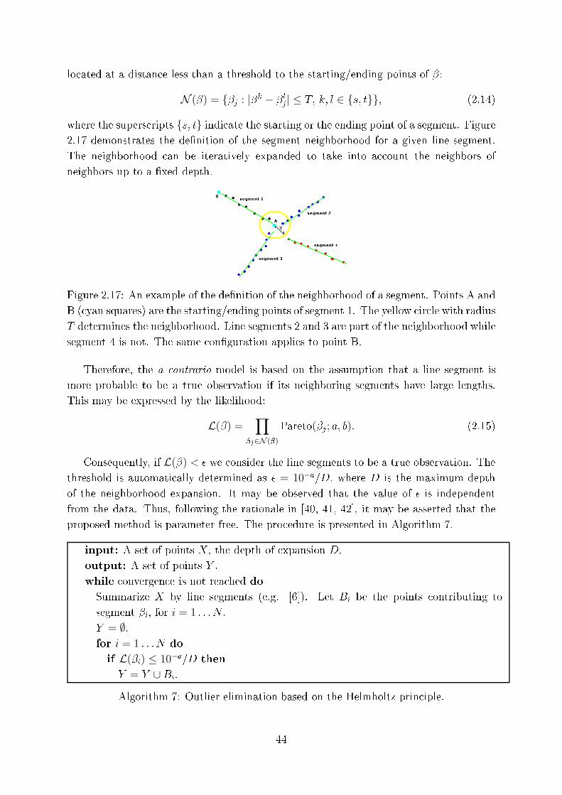
lo ated at a distan e less than a threshold to the starting/ending points of �:

N (�) = {�j

: |�k − �

l

j

| ≤ T; k; l ∈ {s; t}}; (2.14)

where the supers ripts {s; t} indi ate the starting or the ending point of a segment. Figure

2.17 demonstrates the de�nition of the segment neighborhood for a given line segment.

The neighborhood an be iteratively expanded to take into a ount the neighbors of

neighbors up to a �xed depth.

Figure 2.17: An example of the de�nition of the neighborhood of a segment. Points A and

B ( yan squares) are the starting/ending points of segment 1. The yellow ir le with radius

T determines the neighborhood. Line segments 2 and 3 are part of the neighborhood while

segment 4 is not. The same on�guration applies to point B.

Therefore, the a ontrario model is based on the assumption that a line segment is

more probable to be a true observation if its neighboring segments have large lengths.

This may be expressed by the likelihood:

L(�) =∏

�

j

∈N (�)

Pareto(�j

; a; b): (2.15)

Consequently, if L(�) < � we onsider the line segments to be a true observation. The

threshold is automati ally determined as � = 10−a=D, where D is the maximum depth

of the neighborhood expansion. It may be observed that the value of � is independent

from the data. Thus, following the rationale in [40, 41, 42℄, it may be asserted that the

proposed method is parameter free. The pro edure is presented in Algorithm 7.

input: A set of points X, the depth of expansion D.

output: A set of points Y .

while onvergen e is not rea hed do

Summarize X by line segments (e.g. [6℄). Let B

i

be the points ontributing to

segment �

i

, for i = 1 : : :N .

Y = ∅.for i = 1 : : : N do

if L(�i

) ≤ 10−a=D then

Y = Y ∪ Bi

.

Algorithm 7: Outlier elimination based on the Helmholtz prin iple.

44


To investigate the eÆ ien y of the proposed method for outlier elimination, we used

the Gatorbait database [2℄. Degradation of the data set was arti� ially performed in

the following way. For ea h point of the original data set, an outlier was generated by

multiplying the oordinates of that point with a uniformly distributed random number in

the interval (0; 1]. The number of outliers added was set equal to the number of pure data

points. Moreover, the pure data were degraded by zero-mean additive Gaussian noise

with an appropriate standard deviation in order to obtain a signal to noise ratio (SNR)

of 55 dB (e.g. Fig. 2.16(a)). The algorithm was applied to 50 di�erent realizations of

outliers.

We ondu ted omparisons with a density-based method (DBS an [13℄) and the al-

gorithm of Xian hao et al. [12℄. Let us also note that other established methods, su h

as the algorithm in [89℄, were also onsidered but they failed to provide an a eptable

result in our framework of highly orrupted point sets. Finally, we also show the results

of the simple, but in many ases powerful, median �lter for image denoising to highlight

the order of magnitude of the obtained a ura y with respe t to a well known baseline.

To evaluate the results provided by the di�erent algorithms we employed the Hausdor�

distan e between two sets of points X and Y :

dH(X; Y ) = maxx∈X

miny∈Y

{|x− y|}; (2.16)

where X is the original set of points (the ground truth) and Y is the omputed set of

points after outliers removal.

Table 2.8 summarizes the performan e of the ompared methods. As it may be seen,

our method may su essfully re over the initial shape. Its maximum distan e (10:3),

although smaller than the other algorithms, is due to the fa t that, in a few ases, parts

of the pure data were pruned be ause the outliers were lose to them. Moreover, we

examined the sensitivity of our method to parameter a of the Pareto distribution by

applying the algorithm using a variety of values for this parameter, namely a = {2; 3; 4; 5}.As it may be observed, the method is onsistent and its performan e does not depend

on this parameter. Larger values of a may not be employed as the numerator in the

Pareto distribution (2.13) in reases beyond omputer a ura y. As b is the mode of the

distribution, we have set b = 2 in all of the experiments relying on the fa t that we sear h

line segments and any two points de�ne a line segment. This relatively low value for b is

not in favor of our algorithm, as the model a ounts for less populated line segments whi h

generally are due to noise. However, the results showed the robustness of the proposed

approa h.

Furthermore, it is worth noting that DBS an [13℄ needs tedious parameter tuning

(performed here by trial and error) and the method in [12℄ did not dete t many outliers

laying near the shape ontour. Representative results are shown in Fig. 2.18.

A se ond set of experiments addresses the problem of outlier elimination for line �tting.

Following the same prin iples as in the previous experiments, a set of 500 ollinear points

45

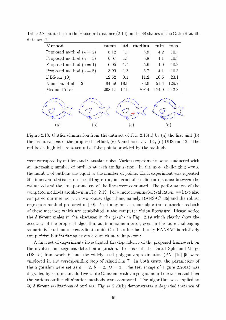
Table 2.8: Statisti s on the Hausdor� distan e (2.16) on the 38 shapes of the GatorBait100

data set [2℄

Method mean std median min max

Proposed method (a = 2) 6.12 1.3 5.8 4.2 10.3




DBS an [13℄ 12.62 3.1 11.2 10.5 23.1

Xian hao et al. [12℄ 84.59 19.6 83.0 51.4 129.7

Median Filter 208.17 17.0 208.4 174.9 243.8

(a) (b) ( ) (d)

Figure 2.18: Outlier elimination from the data set of Fig. 2.16(a) by (a) the �rst and (b)

the last iterations of the proposed method, ( ) Xian hao et al. [12℄, (d) DBS an [13℄. The

red boxes highlight representative false points provided by the methods.

were orrupted by outliers and Gaussian noise. Various experiments were ondu ted with

an in reasing number of outliers at ea h on�guration. In the more hallenging setup,

the number of outliers was equal to the number of points. Ea h experiment was repeated

50 times and statisti s on the �tting error, in terms of Eu lidean distan e between the

estimated and the true parameters of the lines were omputed. The performan es of the

ompared methods are shown in Fig. 2.19. For a more meaningful evaluation, we have also

ompared our method with two robust algorithms, namely RANSAC [36℄ and the robust

regression method proposed in [99℄. As it may be seen, our algorithm outperforms both

of these methods whi h are established in the omputer vision literature. Please noti e

the di�erent s ales in the abs issas in the graphs in Fig. 2.19 whi h learly show the

a ura y of the proposed algorithm as its maximum error, even in the more hallenging

s enario is less than one oordinate unit. On the other hand, only RANSAC is relatively

ompetitive but its �tting errors are mu h more important.

A �nal set of experiments investigated the dependen e of the proposed framework on

the involved line segment dete tion algorithm. To this end, the Dire t Split-and-Merge

(DSaM) framework [6℄ and the widely used polygon approximation (PA) [10℄ [5℄ were

employed in the orresponding step of Algorithm 7. In both ases, the parameters of

the algorithm were set as a = 2, b = 2, D = 3. The test image of Figure 2.20(a) was

degraded by zero-mean additive white Gaussian with varying standard deviation and then

the various outlier elimination methods were ompared. The algorithm was applied to

50 di�erent realizations of outliers. Figure 2.20(b) demonstrates a degraded instan e of

46

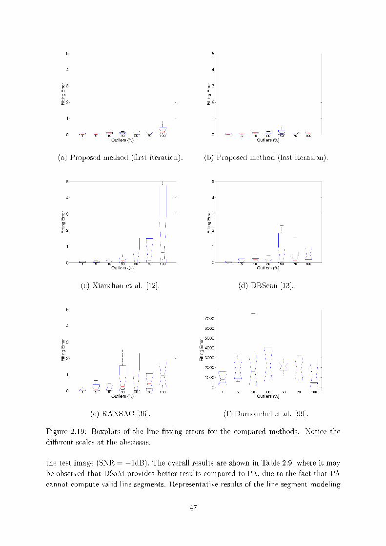
(a) Proposed method (�rst iteration). (b) Proposed method (last iteration).

( ) Xian hao et al. [12℄. (d) DBS an [13℄.

(e) RANSAC [36℄. (f) Dumou hel et al. [99℄.

Figure 2.19: Boxplots of the line �tting errors for the ompared methods. Noti e the

di�erent s ales at the abs issas.

the test image (SNR = −1dB). The overall results are shown in Table 2.9, where it may

be observed that DSaM provides better results ompared to PA, due to the fa t that PA

annot ompute valid line segments. Representative results of the line segment modeling

47

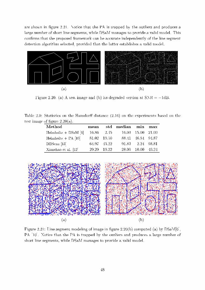
are shown in �gure 2.21. Noti e that the PA is trapped by the outliers and produ es a

large number of short line segments, while DSaM manages to provide a valid model. This

on�rms that the proposed framework an be a urate independently of the line segment

dete tion algorithm sele ted, provided that the latter establishes a valid model.

(a) (b)

Figure 2.20: (a) A test image and (b) its degraded version at SNR = −1dB.

Table 2.9: Statisti s on the Hausdor� distan e (2.16) on the experiments based on the

test image of �gure 2.20(a).

Method mean std median min max

Helmholtz + DSaM [6℄ 16.86 2.45 16.03 15.00 21.00

Helmholtz + PA [10℄ 81.02 19.50 88.41 46.84 94.87

DBS an [13℄ 64.97 43.22 91.83 2.24 98.81

Xian hao et al. [12℄ 29.29 19.22 28.00 10.00 49.24

(a) (b)

Figure 2.21: Line segment modeling of image in �gure 2.20(b) omputed (a) by DSaM[6℄,

PA [10℄. Noti e that the PA is trapped by the outliers and produ es a large number of

short line segments, while DSaM manages to provide a valid model.

48

Part II

Image and Point set Registration

Chapter 3

Registering sets of points using

Bayesian regression

3.1 Introdu tion

3.2 Registration of sets of points via regression

3.3 Experimental Results and Dis ussion

3.1 Introdu tion

Registration of two sets of points is a ommon step in many appli ations in omputer

vision, pattern re ognition, image pro essing and medi al image analysis. The problem

onsists in determining a geometri al transformation that brings two sets of points into

alignment. This ould be a hieved, for instan e, through the establishment of orrespon-

den es. However, the problem is not always well-posed and be omes more ompli ated by

the existen e of noise or outliers, making the determination of orresponden es harder.

Another drawba k rises from the geometri transformation itself, as there may be an in�-

nite number of allowed high dimensional mappings. Also, the de�nition of the similarity

measure is an open issue, sin e one an hoose from a variety of metri s.

Many methods have been proposed to solve the orresponden e problem. A straight-

forward approa h is based on the nearest neighbor riterion to establish orresponden es,

as in the Iterated Closest Point (ICP) algorithm [100℄. However, despite its simpli ity,

this method results in many lo al minima, providing a suboptimal solution, and does not

guarantee that the orresponden e is one-to-one. Many variants of this algorithm have

been proposed improving the behavior of the method in the presen e of noise. A detailed

review an be found in [101℄. Nevertheless, in all ases, ICP methods ne essitate a good

initialization near to the optimal solution in order to prevent the energy fun tion from

getting trapped in lo al minima.

42

The Robust Point Mat hing (RPM) algorithm [14℄ relies on a deterministi annealing

s heme. The algorithm applies the softassign prin iple [102℄ for mat hing and the thin-

plate spline interpolation [15℄ for non-rigid mapping. The rationale is to transfer the

assignment problem from a hard approa h to a soft one, that is to de�ne a probability

for ea h assignment.

The Coherent Point Drift (CPD) algorithm was also proposed in [17℄, where the reg-

istration is treated as a Maximum Likelihood (ML) estimation problem with motion

oheren e onstraints over the velo ity �eld su h that one point set moves oherently in

order to be aligned with the other. In that ase, transformation parameter estimation

and determination of orresponden es are simultaneously handled.

Mixture models were proposed as a framework to solve the registration problem

(GMMReg) [103℄. Ea h set of points is represented by a mixture of Gaussians and reg-

istration is de�ned as a problem of aligning the two mixtures. The L2 metri is used as

a measure of mixture alignment. An extension of the method using robust Student's-t

modeling for the data was also proposed in [104℄.

Shape ontext was onsidered in [105℄, where an iterative algorithm is designed to

a ount for the shape mat hing, registration and dete tion. The problem is formulated in

terms of probabilisti inferen e using a generative model and the EM algorithm. Shape

features are used in a data-driven te hnique to address the problem of initialization.

A te hnique for establishing orresponden es is proposed in [106℄, where features of a

2-D point set whi h are invariant with respe t to a proje tive transformation are extra ted.

The proposed algorithm is based on the omparison of two proje tive and permutation

invariants of �ve-tuples of the points. The best-mat hed �ve-tuples are then used for the

omputation of the proje tive transformation and the one having the maximum number

of orresponding points is used.

Moreover, in [107℄, a novel te hnique is introdu ed to solve the rigid point pattern

mat hing problem in Eu lidean spa es of any dimension. The point pattern mat hing is

modeled as a weighted graph, where nodes represent points and the weights of the edges

are equal to the Eu lidean distan es between nodes. The graph mat hing is formulated

as a problem of �nding a maximum probability on�guration in a graphi al model.

In [108℄, the notion of a neighborhood stru ture for the general point mat hing problem

is introdu ed. Then, the point mat hing problem is formulated as an optimization problem

to preserve lo al neighborhood stru tures during mat hing. The method has a simple

graph mat hing interpretation, where ea h point is a node in the graph, and two nodes

are onne ted by an edge if they are neighbors. The optimal mat h between two graphs

is the one that maximizes the number of mat hed edges.

The majority of the registration methods mentioned so far, model the non-rigid map-

ping through a spline interpolation method, and in parti ular with the thin-plate spline

(TPS) [15℄. In this work, we onsider the transformation parameter estimation issue as

a regression problem and a Bayesian model, namely Relevan e Ve tor Ma hine (RVM)

[109℄ is used to solve this problem. We onsider here the standard RVM although the

43

method may employ other variants su h as the twinned RVM [110℄ whi h applies double

training or the multivariate RVM [111℄.

Our work is motivated by the pioneering resear h presented in [112℄ where orrespon-

den es are estimated using a softassign approa h. Softassign is a te hnique for solving an

assignment problem. As opposed to hard assignment, softassign weights ea h mat hing

to indi ate the quality of the orresponden e. Hard assignment is the limit version of

softassign. In the work herein, instead of solving the assignment problem based on the

smallest distan e, we utilize this distan e to reate a ost matrix that des ribes the ost

of an assignment. Then, the orresponden es are extra ted with a ombinatorial opti-

mization algorithm, the Hungarian algorithm [113℄. The rationale behind this algorithm

is to assign a single task to a single worker, based on an assignment ost matrix, su h

that the total ost is minimum. The temporal omplexity of the algorithm is polynomial,

and in parti ular O(n3). After the orresponden e between points has been established,

a Bayesian regression model (RVM) is used to infer the transformation parameters.

The Hungarian algorithm has also been used in [7℄, where a feature-based registration

method is demonstrated. Points are assumed to des ribe a shape and a histogram (shape

ontext) is al ulated, des ribing the spa e distribution of points. This histogram is used

to de�ne the ost matrix of the Hungarian algorithm. Our work di�erentiates from [7℄

in the way the geometri transformation is treated. We estimate the transformation's

parameters (both rigid and non rigid) through regression (RVM) while the latter method

uses thin plate splines interpolation. Another substantial di�eren e is that in our approa h

points are not onsidered as parts of a shape representation, sin e our method is more

general.

The main ontribution of this work is that using a regression framework based on

RVM addresses the problem of eventual false orresponden es with respe t to methods

relying on interpolation s hemes, like TPS. More pre isely, a single false orresponden e

may lead to a totally erroneous registration if TPS is used. For example, this is a ase

of the RPM [14℄, or the GMMReg [103℄ methods. In �gure 3.1(a), the orre t orrespon-

den es between the sour e and the target sets are represented by line segments. In �gure

3.1(b), two points were falsely mat hed on purpose simulating a wrong orresponden e

solution. The result of TPS [15℄ is shown in �gure 3.1( ), where large registration errors

are present. The result of the proposed registration s heme based on RVM regression

is shown in �gure 3.1(d), where the registration is orre t. TPS by its de�nition tries

to minimize the total bending energy to provide a smooth model, whi h is an approa h

that restri ts the apability of providing good results in areas where the orresponden e

is orre tly established. On the other hand, RVM onsiders only the lo al neighborhood

to extra t the regression model, due to the priors it implies on ea h point. The losed

form solution for the transformation model provided by RVM is ontinuous and lo ally

smooth depending on the assignment solution and more importantly, it is robust to false

mat hes. The orresponden e estimation step used in this work is the Hungarian algo-

rithm. Alternative methods ould also be used to solve the orresponden e problem, like

44

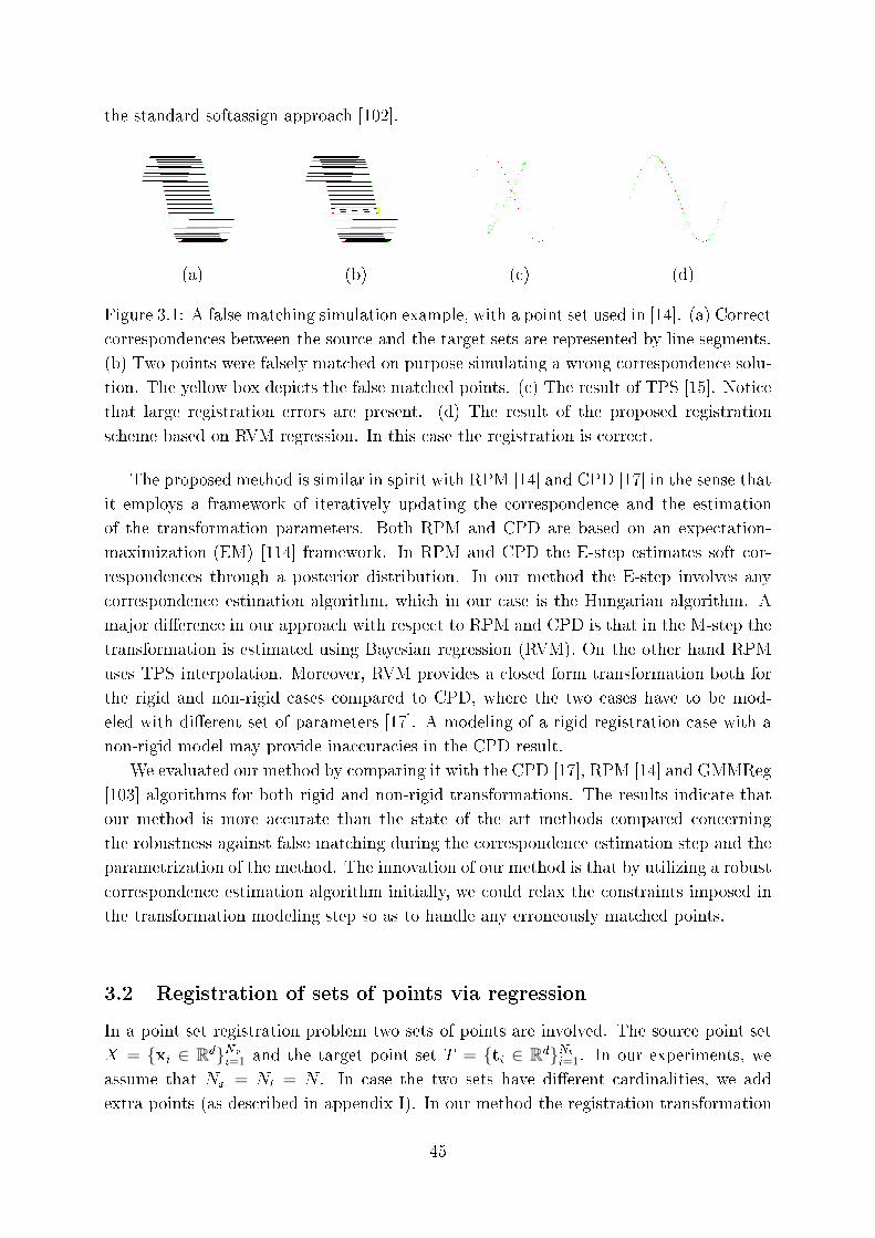
the standard softassign approa h [102℄.

(a) (b) ( ) (d)

Figure 3.1: A false mat hing simulation example, with a point set used in [14℄. (a) Corre t

orresponden es between the sour e and the target sets are represented by line segments.

(b) Two points were falsely mat hed on purpose simulating a wrong orresponden e solu-

tion. The yellow box depi ts the false mat hed points. ( ) The result of TPS [15℄. Noti e

that large registration errors are present. (d) The result of the proposed registration

s heme based on RVM regression. In this ase the registration is orre t.

The proposed method is similar in spirit with RPM [14℄ and CPD [17℄ in the sense that

it employs a framework of iteratively updating the orresponden e and the estimation

of the transformation parameters. Both RPM and CPD are based on an expe tation-

maximization (EM) [114℄ framework. In RPM and CPD the E-step estimates soft or-

responden es through a posterior distribution. In our method the E-step involves any

orresponden e estimation algorithm, whi h in our ase is the Hungarian algorithm. A

major di�eren e in our approa h with respe t to RPM and CPD is that in the M-step the

transformation is estimated using Bayesian regression (RVM). On the other hand RPM

uses TPS interpolation. Moreover, RVM provides a losed form transformation both for

the rigid and non-rigid ases ompared to CPD, where the two ases have to be mod-

eled with di�erent set of parameters [17℄. A modeling of a rigid registration ase with a

non-rigid model may provide ina ura ies in the CPD result.

We evaluated our method by omparing it with the CPD [17℄, RPM [14℄ and GMMReg

[103℄ algorithms for both rigid and non-rigid transformations. The results indi ate that

our method is more a urate than the state of the art methods ompared on erning

the robustness against false mat hing during the orresponden e estimation step and the

parametrization of the method. The innovation of our method is that by utilizing a robust

orresponden e estimation algorithm initially, we ould relax the onstraints imposed in

the transformation modeling step so as to handle any erroneously mat hed points.

3.2 Registration of sets of points via regression

In a point set registration problem two sets of points are involved. The sour e point set

X = {xi

∈ Rd}Nx

i=1 and the target point set T = {ti

∈ Rd}Nt

i=1. In our experiments, we

assume that N

x

= N

t

= N . In ase the two sets have di�erent ardinalities, we add

extra points (as des ribed in appendix I). In our method the registration transformation

45

is modeled by a RVM. However, one would observe that the RVM des ribed in appendix

II is de�ned for univariate output ve tors. In other words, the target variable has to be a

s alar. However, in our ase t

i

∈ Rd

, and thus, in order to over ome this diÆ ulty, we used

d distin t RVMs, one for ea h dimension k. Alternatively, one ould use a multivariate

RVM, as des ribed in [111℄ or the twinned RVM [110℄.

Eventually, the proposed model is a ve tor valued fun tion T , having parameters W ,

representing the geometri transformation bringing setX into alignment with set T . Thus,

ideally we would have for every point t

i

∈ T , i = 1; :::; N :

t

i

= T (xC

i

;W ) = [T 1(xC

i

;w1); :::; T k(xC

i

;wk); :::; T d(xC

i

;wd)]T ; (3.1)

where W = {wk ∈ RN}d

k=1, with wk

being the weight ve tor of dimension N for the k-th

RVM, T k

is a RVM as des ribed by (5.1) in appendix II and C

i

is the index of the point

in X orresponding to the i-th point of T . In other words, the ideal transformation is

t

k

i

= T k(xC

i

;wk) i = 1; : : : ; N; k = 1; : : : ; d (3.2)

with t

k

i

representing the k-th omponent of point t

i

∈ T .

The proposed method onsists of an iterative s heme, that, at ea h iteration alternates

between the method for establishing orresponden es (e.g. Hungarian algorithm) and the

method for estimating the registration transformation (RVM training). The orresponding

obje tive fun tion that is minimized has the following form:

J(Æ;W ) =

N∑

i=1

N∑

j=1

Æ

ij

Cx

i

;T (xj

;W ) +

N∑

i=1

N∑

j=1

Æ

ij

||ti

− T (xj

;W )||2: (3.3)

Its optimization involves two steps at ea h iteration. In the �rst step, we assume a known

registration transformation T (RVM) and try to estimate the optimal orresponden es Æ

ij

with the Hungarian algorithm. Thus, the obje tive fun tion is minimized with respe t to

Æ

ij

, ∀ i; j. In the se ond step, the orresponden es Æ

ij

are �xed to the values omputed in

the �rst step and a RVM training pro ess takes pla e to update the registration transfor-

mation T in order to mat h the estimated orresponden es. Thus, in this se ond step, the

obje tive fun tion is minimized with respe t to the set of weights W = {wk ∈ RN}d

k=1.

Sin e both omputational steps at ea h iteration minimize the obje tive fun tion J , the

whole iterative pro ess onverges to a minimum of J .

The overall pro edure is presented in Algorithm 8. Ea h iteration of the registration

algorithm involves two steps. At �rst, orresponden es between points of the sour e set

X and the target set T are estimated by the Hungarian algorithm and then based on

these orresponden es, d RVMs are trained, one per dimension, to solve the regression

problem of transforming the sour e set to the target set. We initialize the registration

transformation as the identity mapping.

46

1: Initialize the registration transformation as the identity mapping and sele t the type

of basis fun tion �

i

(x), i = 1; :::; N for the RVM.

2: Determine the orresponden es between sets of points X, T .

3: Cal ulate distan e matrix Cij

= ‖T (xi

;W )− t

j

‖ ∀ i = 1; : : :N; j = 1; : : : ; N .

4: Solve the assignment problem with the Hungarian algorithm, where C is an assignment

ost matrix.

5: Transformation parameters estimation - train one RVM per dimension of

point set X.

6: for all RVM

k

, k = 1; : : : ; d do

7: Cal ulate m

k

and �

k

by (5.7) and (5.8).

8: Cal ulate a

k

i

; �

k

;

k

i

by (5.9), (5.10) and (5.11).

9: Iterate steps (3.1) and (3.2) until onvergen e to obtain the new RVM

k

, with w

k =

m

k

.

10: Iterate steps 2, 3 until onvergen e of the obje tive fun tion J(Æ;W ) (3.3).

Algorithm 8: The RVM-Hungarian method for registration of sets of points

3.3 Experimental Results and Dis ussion

In order to evaluate our method, several experiments were ondu ted in a olle tion of

sets of points, �rstly used in [112℄, and widely used in the related literature (�gure 3.2).

The algorithm was tested both for its a ura y and its robustness to noise. Experiments

with real data were also ondu ted. For that purpose we used the 2D range data from [16℄

(�gure 3.3(a)) and the 3D fa e of [17℄ was also used in our experiments (�gure 3.3(b)).

Experiments are divided into two types, a ording to the transformation type (either

rigid or non rigid). In ase of non rigid transformation, the non rigid deformation was

followed by a rigid one, to make the problem more hallenging. In that ase the whole

transformation remains non-rigid. In all ases the registration transformation was ini-

tialized to the identity mapping. The angle of the rigid transformation varied between

[0◦; 10◦], while the translation, varied between [−0:2; 0:2] × [−0:2; 0:2]. The registration

error is de�ned as the Eu lidean distan e between the referen e point and its orrespond-

ing registered. Points of �gure 3.2 range in [0; 1]× [0; 1], while those of �gure 3.3(a) range

in [−40; 10]× [−10; 30] and of �gure's 3.3(b) in [−2; 2]× [−2; 2]× [−2; 2].

In our implementation, di�erent kernels were examined (Gaussian, Student's t-kernel

and Lapla ian) as des ribed in [109℄ and implemented in [115℄. The Lapla ian kernel,

K(x; y) = e

− |x−y|�

, proved to be the most eÆ ient model for the tested input data shown

in �gure 3.2. However, the di�eren es are not onsiderable as the registration a ura ies of

the ompared methods di�er at the third de imal digit. Table 3.1 presents the registration

error statisti s of the rigid ase, while table 3.2 demonstrates the results of the non rigid

ase. In all ases, variable kernel widths were used in the range between 5% and 30% of

the mean varian e of the referen e set. The Lapla ian kernel proved to be less sensitive

to hanges in the variations of the kernel width ompared to the Gaussian and Student's

47

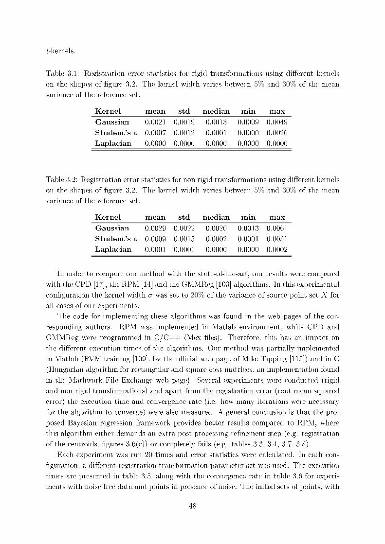
t-kernels.

Table 3.1: Registration error statisti s for rigid transformations using di�erent kernels

on the shapes of �gure 3.2. The kernel width varies between 5% and 30% of the mean

varian e of the referen e set.

Kernel mean std median min max

Gaussian 0.0021 0.0019 0.0013 0.0009 0.0049

Student's t 0.0007 0.0012 0.0001 0.0000 0.0026

Lapla ian 0.0000 0.0000 0.0000 0.0000 0.0000

Table 3.2: Registration error statisti s for non rigid transformations using di�erent kernels

on the shapes of �gure 3.2. The kernel width varies between 5% and 30% of the mean

varian e of the referen e set.

Kernel mean std median min max

Gaussian 0.0029 0.0022 0.0020 0.0013 0.0061

Student's t 0.0009 0.0015 0.0002 0.0001 0.0031

Lapla ian 0.0001 0.0001 0.0000 0.0000 0.0002

In order to ompare our method with the state-of-the-art, our results were ompared

with the CPD [17℄, the RPM [14℄ and the GMMReg [103℄ algorithms. In this experimental

on�guration the kernel width � was set to 20% of the varian e of sour e point set X for

all ases of our experiments.

The ode for implementing these algorithms was found in the web pages of the or-

responding authors. RPM was implemented in Matlab environment, while CPD and

GMMReg were programmed in C/C++ (Mex �les). Therefore, this has an impa t on

the di�erent exe ution times of the algorithms. Our method was partially implemented

in Matlab (RVM training [109℄, by the oÆ ial web page of Mike Tipping [115℄) and in C

(Hungarian algorithm for re tangular and square ost matri es, an implementation found

in the Mathwork File Ex hange web page). Several experiments were ondu ted (rigid

and non rigid transformations) and apart from the registration error (root mean squared

error) the exe ution time and onvergen e rate (i.e. how many iterations were ne essary

for the algorithm to onverge) were also measured. A general on lusion is that the pro-

posed Bayesian regression framework provides better results ompared to RPM, where

this algorithm either demands an extra post pro essing re�nement step (e.g. registration

of the entroids, �gures 3.6( )) or ompletely fails (e.g. tables 3.3, 3.4, 3.7, 3.8).

Ea h experiment was run 20 times and error statisti s were al ulated. In ea h on-

�guration, a di�erent registration transformation parameter set was used. The exe ution

times are presented in table 3.5, along with the onvergen e rate in table 3.6 for experi-

ments with noise free data and points in presen e of noise. The initial sets of points, with

48

representative results are demonstrated in �gure 3.4 for the rigid ase and in �gures 3.5,

3.6 for the non rigid ase. Also, to investigate the robustness of the algorithm to noise,

the points were orrupted by Gaussian noise (with zero mean and small varian e so as

the shape does not hange signi� antly). The initial sets of points, with the estimated

results are demonstrated in �gures 3.8 - 3.11, while the statisti s are presented in tables

3.3 (rigid ase) and 3.4 (non rigid ase) for noise free points and in tables 3.7 (rigid ase)

and 3.8 (non rigid ase) for points orrupted by Gaussian noise with zero mean value. To

further support the statisti al presentation of the registration error results, the p-value

was omputed, so as to verify the statisti al signi� an e of the analysis. Noti e that in

ase of un orrupted data, the deviations between real and omputed values are too small

for all the studied methods, and thus the p-value was not omputed. In the ase of data

orrupted by Gaussian noise, there are di�eren es between the results provided by ea h

method. As it may be observed in the last row of Table 3.7 and Table 3.8, in all ases,

the omputed p-value is less than a threshold of signi� an e level of 5%, whi h is usually

employed.

One an observe that the proposed method, provides better results in general ompared

to CPD, RPM and GMMReg. Observe for example the on entration of estimated target

points in an erroneous spa e (no underlying orresponding sour e points) in �gure 3.6(b)

and �gure 3.6(d), even in the ase of noise free data. The same also applies in ase of

points orrupted by noise, where CPD and GMMReg provided results that des ribe the

shape of the target set quite well but there are points with no underlying orresponden es,

e.g. �gures 3.9 ( ) and 3.9 (e) or �gures 3.10 ( ) and 3.10 (e). On the other hand, RPM

omputed a good mat hing between the registered shapes but a re�nement step is needed

to a hieve perfe t registration, e.g. �gure 3.6( ). In general, RPM proved too diÆ ult to

be tuned, and therefore provided a high rate of failures.

Con erning the CPD and the GMMReg methods, the time omplexity of these algo-

rithms are lower than ours whi h is partially implemented in Matlab (table 3.5). The

fa t that under similar omparison onditions our algorithm may provide similar results

is justi�ed by the onvergen e omparison (table 3.6), where one may observe that our

te hnique onverges quite faster than CPD and GMMReg. A general on lusion regard-

ing the omparison of our method and CPD/GMMReg is, that, taking into a ount the

registration error, the implementation and parameter tuning (e.g. sele ting the type of

transformation rigid or non rigid) along with the time omplexity our method may pro-

vide better registration results, under the ondition that a good assignment solution is

provided.

Another issue studied in our experiments is the integration of an annealing s heme,

either in the orresponden e establishment (step 1 of algorithm 8) or in the RVM training

(step 2 of algorithm 8). One approa h was to embed softassign [102℄, as solution to

the orresponden e establishment instead of the Hungarian algorithm. The annealing

temperature was initialized to 10% of the maximum pairwise distan e between the points.

After ea h iteration, the annealing temperature was redu ed to 0.9 of its previous value.

49

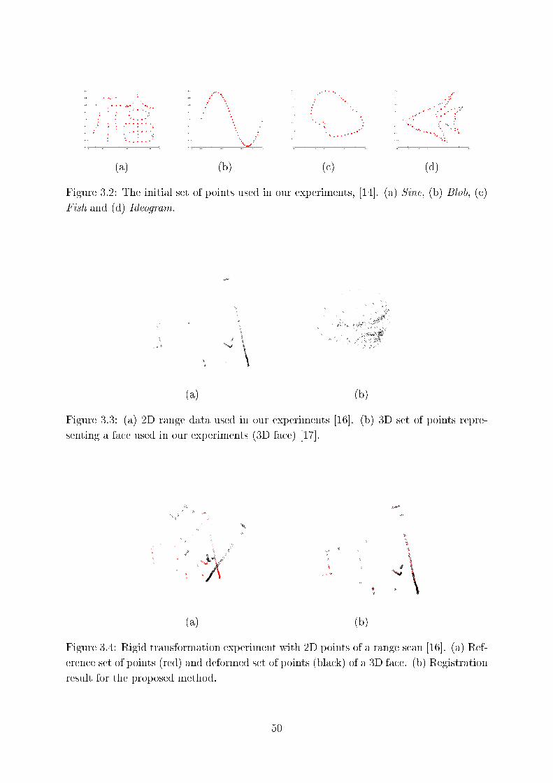
(a) (b) ( ) (d)

Figure 3.2: The initial set of points used in our experiments, [14℄. (a) Sine, (b) Blob, ( )

Fish and (d) Ideogram.

(a) (b)

Figure 3.3: (a) 2D range data used in our experiments [16℄. (b) 3D set of points repre-

senting a fa e used in our experiments (3D fa e) [17℄.

(a) (b)

Figure 3.4: Rigid transformation experiment with 2D points of a range s an [16℄. (a) Ref-

eren e set of points (red) and deformed set of points (bla k) of a 3D fa e. (b) Registration

result for the proposed method.

50

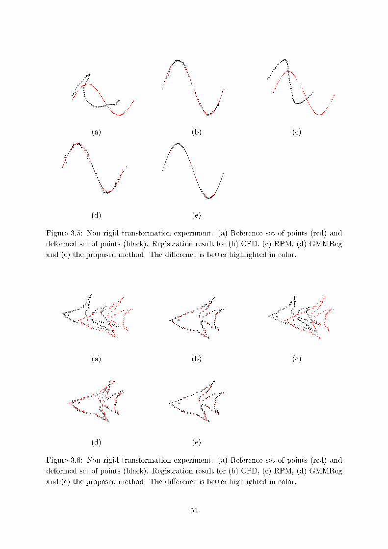
(a) (b) ( )

(d) (e)

Figure 3.5: Non rigid transformation experiment. (a) Referen e set of points (red) and

deformed set of points (bla k). Registration result for (b) CPD, ( ) RPM, (d) GMMReg

and (e) the proposed method. The di�eren e is better highlighted in olor.

(a) (b) ( )

(d) (e)

Figure 3.6: Non rigid transformation experiment. (a) Referen e set of points (red) and

deformed set of points (bla k). Registration result for (b) CPD, ( ) RPM, (d) GMMReg

and (e) the proposed method. The di�eren e is better highlighted in olor.

51

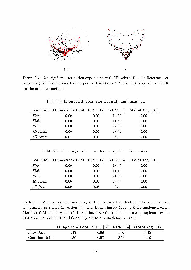
(a) (b)

Figure 3.7: Non rigid transformation experiment with 3D points [17℄. (a) Referen e set

of points (red) and deformed set of points (bla k) of a 3D fa e. (b) Registration result

for the proposed method.

Table 3.3: Mean registration error for rigid transformations.

point set Hungarian-RVM CPD [17℄ RPM [14℄ GMMReg [103℄

Sine 0.00 0.00 14.62 0.00

Blob 0.00 0.00 11.53 0.00

Fish 0.00 0.00 22.60 0.00

Ideogram 0.00 0.00 23.62 0.00

2D range 0.01 0.04 fail 0.00

Table 3.4: Mean registration error for non-rigid transformations.


Sine 0.00 0.00 13.45 0.00

Blob 0.00 0.00 11.19 0.00

Fish 0.00 0.00 21.87 0.00

Ideogram 0.00 0.00 23.50 0.00

3D fa e 0.00 0.08 fail 0.00

Table 3.5: Mean exe ution time (se ) of the ompared methods for the whole set of

experiments presented in se tion 3.3. The Hungarian-RVM is partially implemented in

Matlab (RVM training) and C (Hungarian algorithm). RPM is totally implemented in

Matlab while both CPD and GMMReg are totally implemented in C.

Hungarian-RVM CPD [17℄ RPM [14℄ GMMReg [103℄

Pure Data 0.43 0.08 1.97 0.19

Gaussian Noise 0.30 0.08 2.53 0.49

52

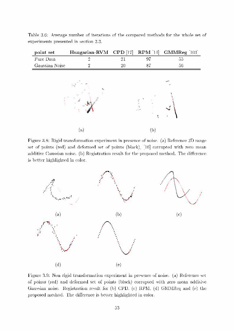
Table 3.6: Average number of iterations of the ompared methods for the whole set of

experiments presented in se tion 3.3.


Pure Data 2 21 97 55

Gaussian Noise 2 20 87 56

(a) (b)

Figure 3.8: Rigid transformation experiment in presen e of noise. (a) Referen e 2D range

set of points (red) and deformed set of points (bla k), [16℄ orrupted with zero mean

additive Gaussian noise. (b) Registration result for the proposed method. The di�eren e

is better highlighted in olor.

(a) (b) ( )

(d) (e)

Figure 3.9: Non rigid transformation experiment in presen e of noise. (a) Referen e set

of points (red) and deformed set of points (bla k) orrupted with zero mean additive

Gaussian noise. Registration result for (b) CPD, ( ) RPM, (d) GMMReg and (e) the

proposed method. The di�eren e is better highlighted in olor.

53

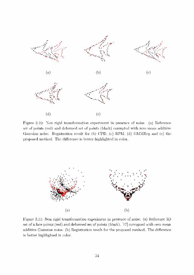
(a) (b) ( )

(d) (e)

Figure 3.10: Non rigid transformation experiment in presen e of noise. (a) Referen e

set of points (red) and deformed set of points (bla k) orrupted with zero mean additive

Gaussian noise. Registration result for (b) CPD, ( ) RPM, (d) GMMReg and (e) the

proposed method. The di�eren e is better highlighted in olor.

(a) (b)

Figure 3.11: Non rigid transformation experiment in presen e of noise. (a) Referen e 3D

set of a fa e points (red) and deformed set of points (bla k), [17℄ orrupted with zero mean

additive Gaussian noise. (b) Registration result for the proposed method. The di�eren e

is better highlighted in olor.

54

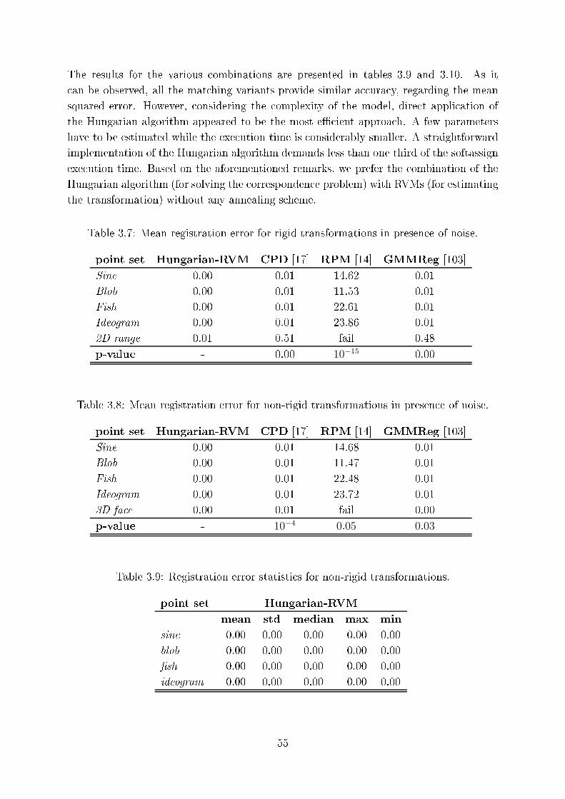
The results for the various ombinations are presented in tables 3.9 and 3.10. As it

an be observed, all the mat hing variants provide similar a ura y, regarding the mean

squared error. However, onsidering the omplexity of the model, dire t appli ation of

the Hungarian algorithm appeared to be the most eÆ ient approa h. A few parameters

have to be estimated while the exe ution time is onsiderably smaller. A straightforward

implementation of the Hungarian algorithm demands less than one third of the softassign

exe ution time. Based on the aforementioned remarks, we prefer the ombination of the

Hungarian algorithm (for solving the orresponden e problem) with RVMs (for estimating

the transformation) without any annealing s heme.

Table 3.7: Mean registration error for rigid transformations in presen e of noise.


Sine 0.00 0.01 14.62 0.01

Blob 0.00 0.01 11.53 0.01

Fish 0.00 0.01 22.61 0.01

Ideogram 0.00 0.01 23.86 0.01

2D range 0.01 0.51 fail 0.48

p-value - 0.00 10−150.00

Table 3.8: Mean registration error for non-rigid transformations in presen e of noise.


Sine 0.00 0.01 14.68 0.01

Blob 0.00 0.01 11.47 0.01

Fish 0.00 0.01 22.48 0.01

Ideogram 0.00 0.01 23.72 0.01

3D fa e 0.00 0.01 fail 0.00

p-value - 10−4 0:05 0:03

Table 3.9: Registration error statisti s for non-rigid transformations.

point set Hungarian-RVM

mean std median max min

sine 0.00 0.00 0.00 0.00 0.00

blob 0.00 0.00 0.00 0.00 0.00

�sh 0.00 0.00 0.00 0.00 0.00

ideogram 0.00 0.00 0.00 0.00 0.00

55

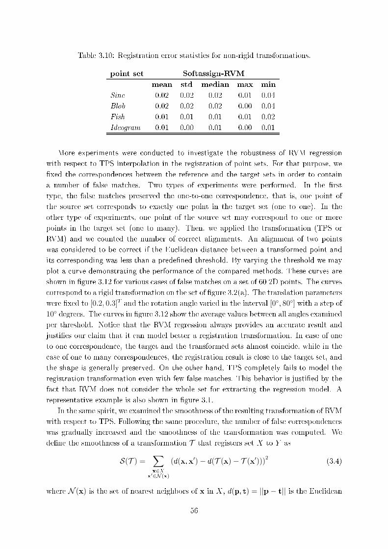
Table 3.10: Registration error statisti s for non-rigid transformations.

point set Softassign-RVM

mean std median max min

Sine 0.02 0.02 0.02 0.01 0.04

Blob 0.02 0.02 0.02 0.00 0.04

Fish 0.01 0.01 0.01 0.01 0.02

Ideogram 0.01 0.00 0.01 0.00 0.01

More experiments were ondu ted to investigate the robustness of RVM regression

with respe t to TPS interpolation in the registration of point sets. For that purpose, we

�xed the orresponden es between the referen e and the target sets in order to ontain

a number of false mat hes. Two types of experiments were performed. In the �rst

type, the false mat hes preserved the one-to-one orresponden e, that is, one point of

the sour e set orresponds to exa tly one point in the target set (one to one). In the

other type of experiments, one point of the sour e set may orrespond to one or more

points in the target set (one to many). Then, we applied the transformation (TPS or

RVM) and we ounted the number of orre t alignments. An alignment of two points

was onsidered to be orre t if the Eu lidean distan e between a transformed point and

its orresponding was less than a prede�ned threshold. By varying the threshold we may

plot a urve demonstrating the performan e of the ompared methods. These urves are

shown in �gure 3.12 for various ases of false mat hes on a set of 60 2D points. The urves

orrespond to a rigid transformation on the set of �gure 3.2(a). The translation parameters

were �xed to [0:2; 0:3]T and the rotation angle varied in the interval [0◦; 80◦] with a step of

10◦ degrees. The urves in �gure 3.12 show the average values between all angles examined

per threshold. Noti e that the RVM regression always provides an a urate result and

justi�es our laim that it an model better a registration transformation. In ase of one

to one orresponden e, the target and the transformed sets almost oin ide, while in the

ase of one to many orresponden es, the registration result is lose to the target set, and

the shape is generally preserved. On the other hand, TPS ompletely fails to model the

registration transformation even with few false mat hes. This behavior is justi�ed by the

fa t that RVM does not onsider the whole set for extra ting the regression model. A

representative example is also shown in �gure 3.1.

In the same spirit, we examined the smoothness of the resulting transformation of RVM

with respe t to TPS. Following the same pro edure, the number of false orresponden es

was gradually in reased and the smoothness of the transformation was omputed. We

de�ne the smoothness of a transformation T that registers set X to Y as

S(T ) =∑

x∈Xx

′∈N (x)

(d(x;x′)− d(T (x)− T (x′)))2

(3.4)

where N (x) is the set of nearest neighbors of x in X, d(p; t) = ||p− t|| is the Eu lidean

56

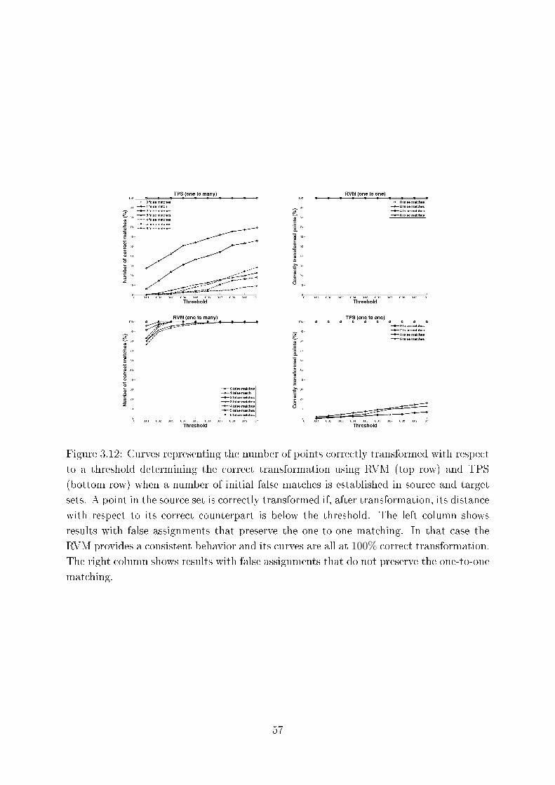
Figure 3.12: Curves representing the number of points orre tly transformed with respe t

to a threshold determining the orre t transformation using RVM (top row) and TPS

(bottom row) when a number of initial false mat hes is established in sour e and target

sets. A point in the sour e set is orre tly transformed if, after transformation, its distan e

with respe t to its orre t ounterpart is below the threshold. The left olumn shows

results with false assignments that preserve the one-to-one mat hing. In that ase the

RVM provides a onsistent behavior and its urves are all at 100% orre t transformation.

The right olumn shows results with false assignments that do not preserve the one-to-one

mat hing.

57

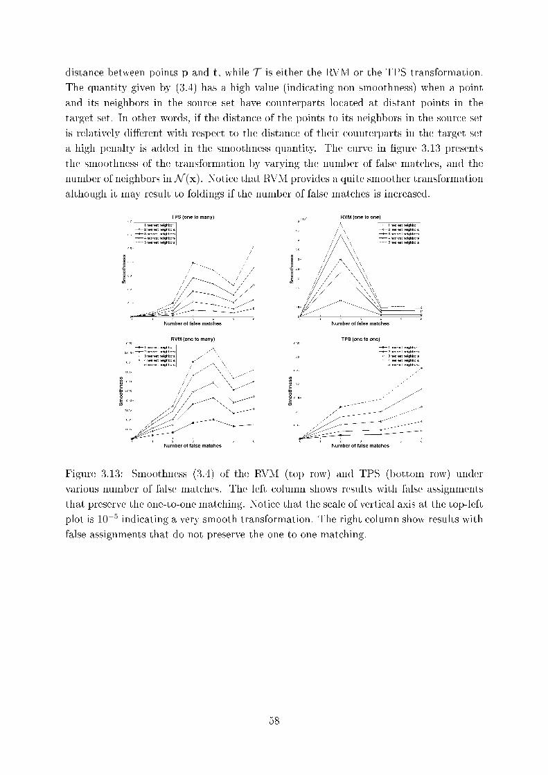
distan e between points p and t, while T is either the RVM or the TPS transformation.

The quantity given by (3.4) has a high value (indi ating non smoothness) when a point

and its neighbors in the sour e set have ounterparts lo ated at distant points in the

target set. In other words, if the distan e of the points to its neighbors in the sour e set

is relatively di�erent with respe t to the distan e of their ounterparts in the target set

a high penalty is added in the smoothness quantity. The urve in �gure 3.13 presents

the smoothness of the transformation by varying the number of false mat hes, and the

number of neighbors inN (x). Noti e that RVM provides a quite smoother transformation

although it may result to foldings if the number of false mat hes is in reased.

Figure 3.13: Smoothness (3.4) of the RVM (top row) and TPS (bottom row) under

various number of false mat hes. The left olumn shows results with false assignments

that preserve the one-to-one mat hing. Noti e that the s ale of verti al axis at the top-left

plot is 10−5indi ating a very smooth transformation. The right olumn show results with

false assignments that do not preserve the one-to-one mat hing.

58

Chapter 4

Registering images and sets of points

using Mixture Models

4.1 Introdu tion

4.2 Image registration with mixtures of Gaussian and Student's t-distributions

4.3 Robust registration of point sets with mixtures of Student's t-distributions

4.4 Experimental results

4.1 Introdu tion

The goal of image registration is to geometri ally align two or more images in order

to superimpose pixels representing the same underlying stru ture. Image registration

is an important preliminary step in many appli ation �elds involving, for instan e, the

dete tion of hanges in temporal image sequen es or the fusion of multimodal images.

For the state of the art of registration methods we refer the reader to [116℄. Medi al

imaging, with its wide variety of sensors (MRI, nu lear, ultrasoni , X-Ray) is probably

one of the �rst appli ation �elds [117, 118, 119℄. Other resear h areas related to image

registration are remote sensing, multisensor robot vision and multisour e imaging used

in the preservation of artisti patrimony. Respe tive appli ations in lude the following of

the evolution of pathologies in medi al image sequen es [120℄, the dete tion of hanges

in urban development from aerial photographs [121℄ and the re overy of underpaintings

from visible/X-ray pairs of images in �ne arts painting analysis [122℄.

The overwhelming majority of hange dete tion or data fusion algorithms assume that

the images to be ompared are perfe tly registered. Even slightly erroneous registrations

may be ome an important sour e of interpretation errors when inter-image hanges have

59

to be dete ted. A urate (i.e. subpixel or subvoxel) registration of single modal images

remains an intri ate problem when gross dissimilarities are observed. The problem is

even more diÆ ult for multimodal images, showing both lo alized hanges that have to

be dete ted and an overall di�eren e due to the variety of responses by multiple sensors.

Sin e the seminal works of Viola and Wells [123℄ and Maes et al. [124℄, the max-

imization of the mutual information measure between a pair of images has gained an

in reasing popularity as a riterion for image registration [125℄. The estimation of both

marginal and joint probability density fun tions of the involved images is a key element

in mutual information based image alignment. However, this method is limited by the

histogram binning problem. Approa hes to over ome this limitation in lude Parzen win-

dowing [123, 126℄, where we have the problem of kernel width spe i� ation, and spline

approximation [127, 128℄. A re ently proposed method relies on the ontinuous represen-

tation of the image fun tion and develops a relation between image intensities and image

gradients along the level sets of the respe tive intensity [129℄.

Gaussian mixture modeling (GMM) [45, 130℄ onstitutes a powerful and exible method

for probabilisti data lustering that is based on the assumption that the data of ea h lus-

ter has been generated by the same Gaussian omponent. In [131℄, GMMs were trained

o�-line to provide prior information on the expe ted joint histogram when the images are

orre tly registered. GMMs have also been su essfully used as models for the joint [132℄

as well as the marginal image densities [133℄, in order to perform intensity orre tion.

They have also been applied in the registration of point sets [134℄ without establishing

expli it orresponden e between points in the two images. The parameters of GMMs an

be estimated very eÆ iently through maximum likelihood (ML) estimation using the EM

algorithm [8℄. Furthermore, it is well-known that GMMs are apable of modeling a large

variety of pdfs [130℄.

An important issue in image registration is the existen e of outlying data due to

temporal hanges (e.g. urban development in satellite images, lesion evolution in medi al

images) or even the omplimentary but non redundant information in pairs of multimodal

images (e.g. visible and infrared data, fun tional and anatomi al medi al images). Al-

though a large variety of image registration methods have been proposed in the literature

only a few te hniques address these ases [135, 120, 136℄.

The method proposed in this study is based on mixture model training. More spe i�-

ally, we train a mixture model on e for the referen e image and obtain the orresponding

partitioning of image pixels into lusters. Ea h luster is represented by the parameters

of the orresponding density omponent. The main idea is that a omponent in the ref-

eren e image orresponds to a omponent in the image to be registered. If the images

are orre tly registered the sum of distan es between the orresponding omponents is

minimum.

A straightforward implementation of the above idea would onsider models with Gaus-

sian omponents. However, it is well known that GMMs are sensitive to outliers and may

lead to ex essive sensitivity when the number of data points is small. This is easily

60

understood by re alling that maximization of the likelihood fun tion under an assumed

Gaussian distribution is equivalent to �nding the least-squares solution whi h la ks ro-

bustness. Consequently, a GMM tends to over-estimate the number of lusters sin e it

uses additional omponents to apture the tails of the distributions [137℄. The problem

of attaining robustness against outliers in multivariate data is diÆ ult and in reases with

the dimensionality. In this work, we onsider mixture models (SMM) with Student's-t

omponents for image registration. This pdf has heavier tails ompared to a Gaussian

[138℄. More spe i� ally, ea h omponent in the SMM mixture originates from a wider

lass of ellipti ally symmetri distributions with an additional parameter alled the num-

ber of degrees of freedom. In this way, a more robust mixture model is employed than

the typi al GMM.

The main ontributions of the proposed registration method are the following: (i)

the histogram binning problem is over ome through image modeling with mixtures of

distributions whi h provide a ontinuous representation of image density. (ii) Robustness

to outlying pixel values is a hieved by using mixtures of Student's t-distributions. The

widely used method of maximization of the mutual information is outperformed. (iii)

The method may be dire tly applied to ve tor valued images (e.g. di�usion tensor MRI)

where standard histogram-based methods fail due to the urse of dimensionality. (iv)

The proposed method is faster than histogram based methods where the joint histogram

needs to be omputed for every hange in the transformation parameters.

Moreover, the registration problem is extended to the ase of point sets where the

nature of the problem is di�erent sin e there is no spatial ordering ontrary to image grids

(e.g. pixelized images). Therefore, the diÆ ulty onsists in simultaneously estimating the

transformation parameters and establishing orresponden es between points.

In the related literature of point set registration, the standard approa h is the well

known Iterative Closest Points (ICP) algorithm [100℄ and its variants [101, 139, 140, 141℄.

In [14, 112℄ a robust point mat hing algorithm is proposed relying on soft-assign [142℄

and an iterative optimization pro edure. The soft-assign is based on a matrix whose

entries des ribe the probability that a point of one set mat hes upon transformation to

one of the other set. Mutual information was also used as a onstraint [143℄ for point

set mat hing under the above framework. Features extra ted from the point sets are

employed in [7, 105℄, a kernel-based method is used in [144℄ and a method modeling the

point sets by a GMM with onstraints on the omponent enters is presented in [145℄.

Also, an approa h to the onstru tion of an atlas from multiple point sets is proposed in

[146℄. Finally, a work related to the herein proposed approa h is presented in [134℄. The

authors propose to model the probability density fun tion (pdf) of the points of the two

sets by GMMs and estimate the transformation parameters through the minimization of

an energy fun tion des ribing the distan e of the two GMMs. Our model ompletes this

study by proposing a more robust framework for modeling the point sets.

61

4.2 Image registration with mixtures of Gaussian and Student's

t-distributions

Let I

ref

be an image of N × N pixels with intensities denoted as I

ref

(xi), where xi,

i = 1; :::; N2, is the i

th

pixel index. The purpose of rigid image registration is to esti-

mate a set of parameters S of the rigid transformation TS minimizing a ost fun tion

E(Iref

(·); Ireg

(TS(·))) that, in a similarity metri -based ontext, expresses the similarity

between the image pair. In the 2D ase the rigid transformation parameters are the ro-

tation angle and the translation parameters along the two axes. In the 3D ase, there

are three rotation and three translation parameters. Eventually, s ale fa tors may also be

in luded, depending on the de�nition of the transformation.

Consider, now, a partitioning of the referen e image I

ref

into K lusters (groups) by

training a mixture model with K omponents with arbitrary pdf p(I(x); Θ):

�(Iref

(x)) =

K∑

k=1

�

k

p(Iref

(x); Θref

k

)

Therefore, the referen e image is represented by the parameters Θref

k

, k = 1; : : : ; K of

the mixture omponents. The partitioning of the image is des ribed using the fun tion

f(x) : [1; 2; :::; N ] × [1; 2; :::; N ] → {1; 2; :::; K}, where f(x) = k means that pixel x of

the referen e image I

ref

belongs to the luster de�ned by the k

th

omponent. Let us also

de�ne the sets of all pixels of image I

ref

belonging to the k

th

luster:

P

k

= {xi ∈ I

ref

; i = 1; 2; :::; N2|Æ(f(xi)− k) = 1}

for k = 1; :::; K, where Æ(x) is the Dira fun tion:

Æ(f(xi)− k) =

{

1; if f(xi) = k

0; otherwise

(4.1)

The above mixture-based segmentation of the referen e image is performed on e, at

the beginning of the registration pro edure. The referen e image I

ref

is, thus, partitioned

into K groups, generally, not orresponding to onne ted omponents in the image. This

spatial partition is proje ted on the image to be registered I

reg

, yielding a orresponding

partition of this se ond image (i.e., the partitioning of the referen e image a ts as a mask

on the image to be registered). Then, we assume that the pixel values of ea h luster k

in I

reg

are modeled using a mixture omponent with parameters Θreg

k

obtained from the

statisti s of the intensities of pixels in group k of I

reg

.

In order to apply our method it should be possible to de�ne a distan e measure

D(Θref

k

;Θreg

k

) between the orresponding mixture omponents with pdf p(I). Then the

energy fun tion we propose, is expressed by the weighted sum of distan es between the

orresponding omponents in I

reg

and I

ref

:

E(Iref

(·); Ireg

(TS(·))) =K∑

k=1

�

k

D(Θref

k

;Θreg

k

) (4.2)

62

where �

k

is the mixing proportion of the k

th

omponent:

�

k

=|P

k

|K∑

l=1

|Pl

|

where |Pk

| denotes the ardinality of set Pk

. If the two images are orre tly registered the

riterion in (4.2) assumes that the total distan e between the whole set of omponents

would be minimum.

For a given set of transformation parameters S, the total energy between the image

pair is omputed through the following steps:

• segment the referen e image I

ref

(·) into K lusters by a mixture model.

• for ea h luster k = 1; 2; :::; K of the referen e image:

{ proje t the pixels of the luster onto the transformed image to be registered

I

reg

(TS(·)).{ determine the parameters Θreg

k

of the proje ted partition of I

reg

.

• evaluate the energy in eq. (4.2) by omputing the distan es between the orrespond-

ing densities.

In the ase of GMMs, the above registration pro edure an be applied as follows:

Consider the multivariate normal distributions N1(�1;Σ1) and N2(�2;Σ2) and denote

Θi

= {�i

;Σi

}, with i = {1; 2}, their respe tive parameters (mean ve tor and ovarian e

matrix). The Cherno� distan e between these distributions is de�ned as [147℄:

C(Θ1;Θ2; s) =s(1− s)

2(�2 − �1)

T [sΣ1 + (1− s)Σ2]−1(�2 − �1)

+1

2ln

( |sΣ1 + (1− s)Σ2||Σ1|s|Σ2|1−s

)

:

The Bhatta haryya distan e is a spe ial ase of the Cherno� distan e with s = 0:5:

B(Θ1;Θ2) =1

8(�2 − �1)

T

[Σ1 + Σ2

2

]−1

(�2 − �1) +1

2ln

(

|Σ1+Σ2

2|

√

|Σ1||Σ2|

)

(4.3)

A representative GMM for the referen e image an be obtained via the EM algorithm

[45℄. Therefore, the referen e image is represented by the parameters Θref

k

= {�refk

;Σref

k

},k = 1; : : : ; K of the GMM omponents. After proje ting the pixel groups of the referen e

image to obtain the orresponding groups in the registered image, the parameters Θreg

k

an be estimated by taking the sample mean �

reg

k

and the sample ovarian e matrix Σreg

k

:

�

reg

k

=1

|Pk

|N

2∑

i=1

I

reg

(TS(xi))Æ(f(xi)− k) (4.4)

63

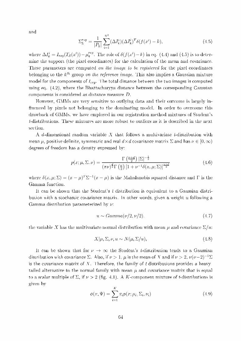
and

Σreg

k

=1

|Pk

|N

2∑

i=1

(∆I ik

)(∆I ik

)T Æ(f(xi)− k); (4.5)

where ∆I ik

= I

reg

(TS(xi))−�reg

k

. The role of Æ(f(xi)−k) in eq. (4.4) and (4.5) is to deter-mine the support (the pixel oordinates) for the al ulation of the mean and ovarian e.

These parameters are omputed on the image to be registered for the pixel oordinates

belonging to the k

th

group on the referen e image. This also implies a Gaussian mixture

model for the omponents of I

reg

. The total distan e between the two images is omputed

using eq. (4.2), where the Bhatta haryya distan e between the orresponding Gaussian

omponents is onsidered as distan e measure D.

However, GMMs are very sensitive to outlying data and their out ome is largely in-

uen ed by pixels not belonging to the dominating model. In order to over ome this

drawba k of GMMs, we have employed in our registration method mixtures of Student's

t-distributions. These mixtures are more robust to outliers as it is des ribed in the next

se tion.

A d-dimensional random variable X that follows a multivariate t-distribution with

mean �, positive de�nite, symmetri and real d×d ovarian e matrix Σ and has � ∈ [0;∞)

degrees of freedom has a density expressed by:

p(x;�;Σ; �) =Γ(�+d2

)|Σ|− 1

2

(��)d

2Γ(�

2

)[1 + �

−1Æ(x; �; Σ)]

�+d

2

(4.6)

where Æ(x; �; Σ) = (x− �)TΣ−1(x− �) is the Mahalanobis squared distan e and Γ is the

Gamma fun tion.

It an be shown that the Student's t distribution is equivalent to a Gaussian distri-

bution with a sto hasti ovarian e matrix. In other words, given a weight u following a

Gamma distribution parameterized by �:

u ∼ Gamma(�=2; �=2): (4.7)

the variable X has the multivariate normal distribution with mean � and ovarian e Σ=u:

X|�;Σ; �; u ∼ N(�;Σ=u); (4.8)

It an be shown that for � → ∞ the Student's t-distribution tends to a Gaussian

distribution with ovarian e Σ. Also, if � > 1, � is the mean ofX and if � > 2, �(�−2)−1Σ

is the ovarian e matrix of X. Therefore, the family of t-distributions provides a heavy-

tailed alternative to the normal family with mean � and ovarian e matrix that is equal

to a s alar multiple of Σ, if � > 2 (�g. 4.1). A K- omponent mixture of t-distributions is

given by

�(x;Ψ) =K∑

i=1

�

i

p(x;�i

;Σi

; �

i

) (4.9)

64

−5 −4 −3 −2 −1 0 1 2 3 4 50

0.05

0.1

0.15

0.2

0.25

0.3

0.35

0.4

x

p(x)

ν=0.1ν=1ν=10

Figure 4.1: A univariate Student's t-distribution (� = 0, � = 1) for various degrees of

freedom. As � → ∞ the distribution tends to a Gaussian. For small values of � the

distribution has heavier tails than a Gaussian.

where x = (x1; :::; xN)T

denotes the observed-data ve tor and

Ψ = (�1; :::; �K ; �1; :::; �K;Σ1; :::;ΣK

; �1; :::; �K)T

: (4.10)

are the parameters of the omponents of the mixture.

A Student's t-distribution mixture model (SMM) may also be trained using the EM

algorithm [138℄. Consider now the omplete data ve tor

x

= (x1; :::xN ; z1; :::; zN ; u1; :::; uN)T

(4.11)

where z1; :::; zN are the omponent-label ve tors and z

ij

= (zj

)i

is either one or zero,

a ording to whether the observation x

j

is generated or not by the i

th

omponent. In the

light of the de�nition of the t-distribution, it is onvenient to view that the observed data

augmented by the z

j

, j = 1; :::; N are still in omplete be ause the omponent ovarian e

matri es depend on the degrees of freedom. This is the reason that the omplete-data

ve tor also in ludes the additional missing data u1; :::; uN . Thus, the E-step on the (t+1)th

iteration of the EM algorithm requires the al ulation of the posterior probability that

the datum x

j

belongs to the i

th

omponent of the mixture:

z

t+1ij

=�

t

i

p(xj

;�ti

;Σt

i

; �

t

i

)K∑

m=1

�

t

m

p(xj

;�tm

;Σt

m

; �

t

m

)

(4.12)

as well as the expe tation of the weights for ea h observation:

u

t+1ij

=�

t

i

+ d

�

t

i

+ Æ(xj

; �

t

i

; Σt

i

)(4.13)

Maximizing the log-likelihood of the omplete data provides the update equations of

the respe tive mixture model parameters:

�

t+1i

=1

N

N∑

j=1

z

t

ij

; (4.14)

65

�

t+1i

=

N∑

j=1

z

t

ij

u

t

ij

x

j

N∑

j=1

z

t

ij

u

t

ij

; (4.15)

Σt+1i

=

N∑

j=1

z

t

ij

u

t

ij

(xj

− �

t+1i

)(xj

− �

t+1i

)T

N∑

j=1

z

t+1ij

: (4.16)

The degrees of freedom �

t+1i

for the i

th

omponent, at time step t + 1, are omputed as

the solution to the equation:

log

(�

t+1i

2

)

−

(�

t+1i

2

)

+ 1− log

(�

t

i

+ d

2

)

+

N∑

j=1

z

t

ij

(log utij

− u

t

ij

)

N∑

j=1

z

t

ij

+

(�

t

i

+ d

2

)

= 0

(4.17)

where (x) = �(lnΓ(x))�x

is the digamma fun tion.

At the end of the algorithm, the data are assigned to the omponent with maximum

responsibility using a maximum a posteriori (MAP) prin iple.

The Student's t-distribution is a heavy tailed approximation to the Gaussian. It

is therefore, natural to onsider the mean and ovarian e of the SMM omponents to

approximate the parameters of a GMM on the same data as it was des ribed in the

previous se tion. If the statisti s of the images follow a Gaussian model, the degrees of

freedom �

i

are relatively large and the SMM tends to be a GMMwith the same parameters.

If the images ontain outliers, parameters �

i

are weak and the mean and ovarian e of the

data are appropriately weighted in order not to take into a ount the outliers. Thus, the

parameters of the SMM, omputed on the referen e image I

ref

, are used as omponent

parameters Θref

k

in a straightforward way as they generalize the Gaussian ase by orre tly

addressing the outliers problem. After proje tion of the pixel groups of the referen e image

to their orresponding groups in the registered image, the parameters Θreg

k

are omputed

using the sample mean (4.4) and the sample ovarian e matrix (4.5).

On e model inferen e is a omplished, the Bhatta haryya distan e between the om-

ponents of the Student's t-mixtures is minimized. The di�eren e with respe t to the GMM

is that the ovarian e matri es are properly s aled by the Gamma distributed parameters

u as it is de�ned in equations (4.7)-(4.8).

Finally, let us noti e that the energy in (4.2) may be applied to both single and

multimodal image registration. In the latter ase, the di�eren e in the mean values of the

distributions in (4.3) should be ignored, as we do not sear h to mat h the orresponding

Student's t-distributions in position but only in shape. In that ase, the distan e in (4.3)

66

be omes:

B(Θ1;Θ2) = ln

(

|Σ1+Σ2

2|

√

|Σ1||Σ2|

)

(4.18)

whi h is equivalent to a orrelation oeÆ ient between the two distributions.

4.3 Robust registration of point sets with mixtures of Student's

t-distributions

An extension of the registration algorithm to handle point sets is des ribed in this se tion.

Given two sets of points X and Y su h that Y is derived from X after applying a rigid

transformation TS with parameters S, that is Y = TS(X), the problem onsists in esti-

mating the transformation parameters from the two data sets without prior knowledge on

any orresponden e. In fa t, in our formulation, there ould be no exa t orresponden e

at all due to noise or outlying points.

Let us denote p(x) the density at a point x ∈ X and assume that it is expressed by a

GMM of M omponents:

p(x) =M∑

j=1

�

x

j

N (x|�xj

;Σx

j

): (4.19)

By the same assumption, the density at a point y ∈ Y is given by another GMM:

q(y) =

N∑

j=1

�

y

j

N (y|�yj

;Σy

j

): (4.20)

Considering the transformed point set distribution as p

R;t

(x), where R is the rotation

matrix ant t is the translation ve tor, that is

p

R;t

(x) =M∑

i=1

�

x

i

N (x|R�xi

+ t; RΣx

i

R

T ); (4.21)

we seek to minimize the energy fun tion:

D(pR;t

; q) =

∫

[pR;t

(z)− q(z)]2dz (4.22)

with respe t to R and t. More spe i� ally, we seek to mat h the ontinuous shapes of the

mixtures p

R;t

and q over their region of support. Equation (4.22) may be simpli�ed:

D(pR;t

; q) =

∫[p

2R;t

(z) + q

2(z)− 2pR;t

(z)q(z)]dz (4.23)

The �rst two terms are invariant under rigid transformation and therefore, the above

expression yields the maximum of the produ t of the two distributions over the whole

67

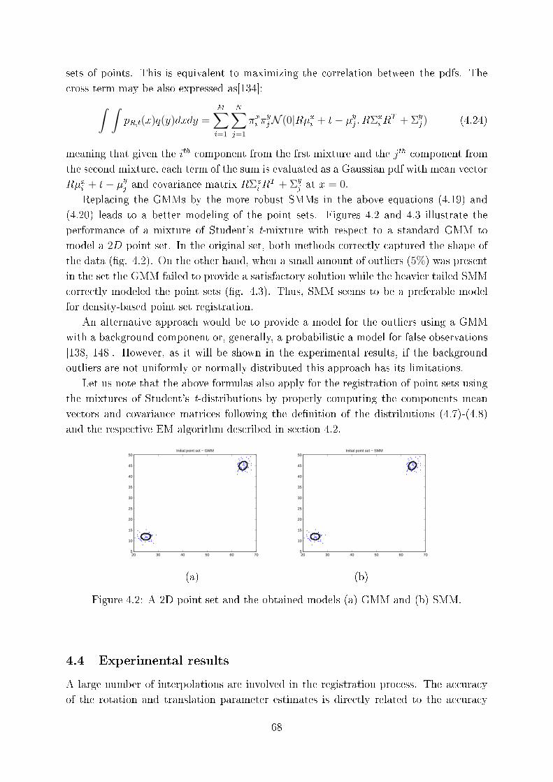
sets of points. This is equivalent to maximizing the orrelation between the pdfs. The

ross term may be also expressed as[134℄:

∫ ∫

p

R;t

(x)q(y)dxdy =M∑

i=1

N∑

j=1

�

x

i

�

y

j

N (0|R�xi

+ t− �

y

j

; RΣx

i

R

T + Σy

j

) (4.24)

meaning that given the i

th

omponent from the frst mixture and the j

th

omponent from

the se ond mixture, ea h term of the sum is evaluated as a Gaussian pdf with mean ve tor

R�

x

i

+ t− �

y

j

and ovarian e matrix RΣx

i

R

T + Σy

j

at x = 0.

Repla ing the GMMs by the more robust SMMs in the above equations (4.19) and

(4.20) leads to a better modeling of the point sets. Figures 4.2 and 4.3 illustrate the

performan e of a mixture of Student's t-mixture with respe t to a standard GMM to

model a 2D point set. In the original set, both methods orre tly aptured the shape of

the data (�g. 4.2). On the other hand, when a small amount of outliers (5%) was present

in the set the GMM failed to provide a satisfa tory solution while the heavier tailed SMM

orre tly modeled the point sets (�g. 4.3). Thus, SMM seems to be a preferable model

for density-based point set registration.

An alternative approa h would be to provide a model for the outliers using a GMM

with a ba kground omponent or, generally, a probabilisti a model for false observations

[138, 148℄. However, as it will be shown in the experimental results, if the ba kground

outliers are not uniformly or normally distributed this approa h has its limitations.

Let us note that the above formulas also apply for the registration of point sets using

the mixtures of Student's t-distributions by properly omputing the omponents mean

ve tors and ovarian e matri es following the de�nition of the distributions (4.7)-(4.8)

and the respe tive EM algorithm des ribed in se tion 4.2.

20 30 40 50 60 705

10

15

20

25

30

35

40

45

50Initial point set − GMM

20 30 40 50 60 705

10

15

20

25

30

35

40

45

50Initial point set − SMM

(a) (b)

Figure 4.2: A 2D point set and the obtained models (a) GMM and (b) SMM.

4.4 Experimental results

A large number of interpolations are involved in the registration pro ess. The a ura y

of the rotation and translation parameter estimates is dire tly related to the a ura y

68

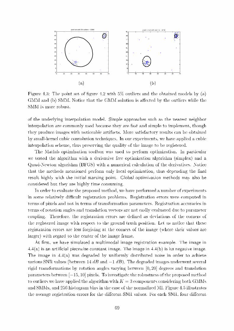
0 10 20 30 40 50 60 700

5

10

15

20

25

30

35

40

45

50point set with 5% outliers − GMM

(a) (b)

Figure 4.3: The point set of �gure 4.2 with 5% outliers and the obtained models by (a)

GMM and (b) SMM. Noti e that the GMM solution is a�e ted by the outliers while the

SMM is more robust.

of the underlying interpolation model. Simple approa hes su h as the nearest neighbor

interpolation are ommonly used be ause they are fast and simple to implement, though

they produ e images with noti eable artifa ts. More satisfa tory results an be obtained

by small-kernel ubi onvolution te hniques. In our experiments, we have applied a ubi

interpolation s heme, thus preserving the quality of the image to be registered.

The Matlab optimization toolbox was used to perform optimization. In parti ular

we tested the algorithm with a derivative free optimization algorithm (simplex) and a

Quasi-Newton algorithm (BFGS) with a numeri al al ulation of the derivatives. Noti e

that the methods mentioned perform only lo al optimization, thus depending the �nal

result highly with the initial starting point. Global optimization methods may also be

onsidered but they are highly time onsuming.

In order to evaluate the proposed method, we have performed a number of experiments

in some relatively diÆ ult registration problems. Registration errors were omputed in

terms of pixels and not in terms of transformation parameters. Registration a ura ies in

terms of rotation angles and translation ve tors are not easily evaluated due to parameter

oupling. Therefore, the registration errors are de�ned as deviations of the orners of

the registered image with respe t to the ground truth position. Let us noti e that these

registration errors are less forgiving at the orners of the image (where their values are

larger) with regard to the enter of the image frame.

At �rst, we have simulated a multimodal image registration example. The image in

4.4(a) is an arti� ial pie ewise onstant image. The image in 4.4(b) is its negative image.

The image in 4.4(a) was degraded by uniformly distributed noise in order to a hieve

various SNR values (between 14 dB and −1 dB). The degraded images underwent several

rigid transformations by rotation angles varying between [0; 20] degrees and translation

parameters between [−15; 10] pixels. To investigate the robustness of the proposed method

to outliers we have applied the algorithm withK = 3 omponents onsidering both GMMs

and SMMs, and 256 histogram bins in the ase of the normalized MI. Figure 4.5 illustrates

the average registration errors for the di�erent SNR values. For ea h SNR, four di�erent

69

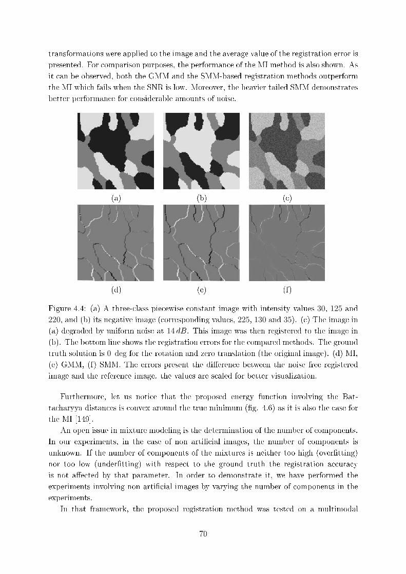
transformations were applied to the image and the average value of the registration error is

presented. For omparison purposes, the performan e of the MI method is also shown. As

it an be observed, both the GMM and the SMM-based registration methods outperform

the MI whi h fails when the SNR is low. Moreover, the heavier tailed SMM demonstrates

better performan e for onsiderable amounts of noise.

(a) (b) ( )

(d) (e) (f)

Figure 4.4: (a) A three- lass pie ewise onstant image with intensity values 30, 125 and

220, and (b) its negative image ( orresponding values, 225, 130 and 35). ( ) The image in

(a) degraded by uniform noise at 14 dB. This image was then registered to the image in

(b). The bottom line shows the registration errors for the ompared methods. The ground

truth solution is 0 deg for the rotation and zero translation (the original image). (d) MI,

(e) GMM, (f) SMM. The errors present the di�eren e between the noise free registered

image and the referen e image. the values are s aled for better visualization.

Furthermore, let us noti e that the proposed energy fun tion involving the Bat-

ta haryya distan es is onvex around the true minimum (�g. 4.6) as it is also the ase for

the MI [149℄.

An open issue in mixture modeling is the determination of the number of omponents.

In our experiments, in the ase of non arti� ial images, the number of omponents is

unknown. If the number of omponents of the mixtures is neither too high (over�tting)

nor too low (under�tting) with respe t to the ground truth the registration a ura y

is not a�e ted by that parameter. In order to demonstrate it, we have performed the

experiments involving non arti� ial images by varying the number of omponents in the

experiments.

In that framework, the proposed registration method was tested on a multimodal

70

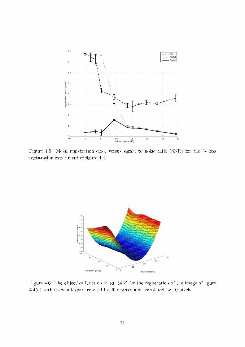
−5 0 5 10 15 20 25 300

1

2

3

4

5

6

7

8

Uniform Noise (dB)

regi

stra

tion

erro

r (p

ixel

s)

MIGMMSMM

Figure 4.5: Mean registration error versus signal to noise ratio (SNR) for the 3- lass

registration experiment of �gure 4.4.

0

10

20

30

40

0

10

20

30

403.5

4

4.5

5

5.5

6

6.5

7

7.5

8

Rotation (degrees)Translation (pixels)

Bat

tach

arry

a di

stan

ce

Figure 4.6: The obje tive fun tion in eq. (4.2) for the registration of the image of �gure

4.4(a) with its ounterpart rotated by 20 degrees and translated by 10 pixels.

71

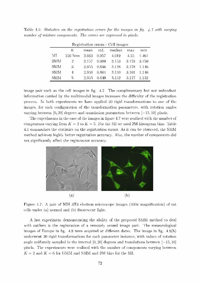
Table 4.1: Statisti s on the registration errors for the images in �g. 4.7 with varying

number of mixture omponents. The errors are expressed in pixels.

Registration errors - Cell images

K mean std. median max min

MI 256 bins 3.663 0.957 4.019 4.25 1.461

SMM 2 3.157 0.009 3.153 3.178 3.150

SMM 3 2.955 0.636 3.148 3.178 1.146

SMM 4 2.956 0.604 3.159 3.101 1.146

SMM 5 2.953 0.640 3.152 3.177 1.132

image pair su h as the ell images in �g. 4.7. The omplimentary but not redundant

information arried by the multimodal images in reases the diÆ ulty of the registration

pro ess. In both experiments we have applied 20 rigid transformations to one of the

images, for ea h on�guration of the transformation parameters, with rotation angles

varying between [0; 20] degrees and translation parameters between [−15; 10] pixels.

The experiments in the ase of the images in �gure 4.7 were realized with the number of

omponents varying from K = 2 to K = 5. For the MI we used 256 histogram bins. Table

4.1 summarizes the statisti s on the registration errors. As it an be observed, the SMM

method a hieves highly better registration a ura y. Also, the number of omponents did

not signi� antly a�e t the registration a ura y.

(a) (b)

Figure 4.7: A pair of NIH 3T3 ele tron mi ros ope images (400x magni� ation) of rat

ells under (a) normal and (b) uores ent light.

A last experiment demonstrating the ability of the proposed SMM method to deal

with outliers is the registration of a remotely sensed image pair. The meteorologi al

images of Europe in �g. 4.8 were a quired at di�erent dates. The image in �g. 4.8(b)

underwent 20 rigid transformations for ea h parameter instan e, with values of rotation

angle uniformly sampled in the interval [0; 20] degrees and translations between [−15; 10]

pixels. The experiments were realized with the number of omponents varying between

K = 2 and K = 6 for GMM and SMM and 256 bins for the MI.

72

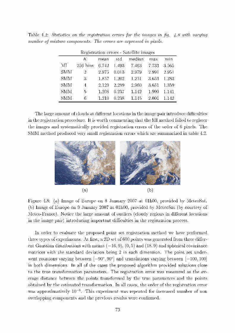
Table 4.2: Statisti s on the registration errors for the images in �g. 4.8 with varying

number of mixture omponents. The errors are expressed in pixels.

Registration errors - Satellite images

K mean std median max min

MI 256 bins 6.742 1.493 7.463 7.733 3.565

SMM 2 2.975 0.013 2.979 2.991 2.951

SMM 3 1.857 1.202 1.251 3.653 1.283

SMM 4 2.129 2.289 2.960 3.651 1.359

SMM 5 1.208 0.237 1.142 1.999 1.141

SMM 6 1.210 0.238 1.145 2.001 1.142

The large amount of louds at di�erent lo ations in the image pair introdu e diÆ ulties

in the registration pro edure. It is worth ommenting that the MI method failed to register

the images and systemati ally provided registration errors of the order of 6 pixels. The

SMM method produ ed very small registration errors whi h are summarized in table 4.2.

(a) (b)

Figure 4.8: (a) Image of Europe on 8 January 2007 at 01h00, provided by MeteoSat.

(b) Image of Europe on 9 January 2007 at 01h00, provided by MeteoSat (by ourtesy of

Meteo-Fran e). Noti e the large amount of outliers ( loudy regions in di�erent lo ations

in the image pair) introdu ing important diÆ ulties in the registration pro ess.

In order to evaluate the proposed point set registration method we have performed

three types of experiments. At �rst, a 2D set of 600 points was generated from three di�er-

ent Gaussian distributions with means (−16; 9), (0; 5) and (18; 9) and spheri al ovarian e

matri es with the standard deviation being 2 in ea h dimension. The point set under-

went rotations varying between [−90◦; 90◦] and translations varying between [−100; 100]

in both dimensions. In all of the ases the proposed algorithm provided solutions lose

to the true transformation parameters. The registration error was measured as the av-

erage distan e between the points transformed by the true parameters and the points

obtained by the estimated transformation. In all ases, the order of the registration error

was approximatively 10−6. This experiment was repeated for in reased number of non

overlapping omponents and the previous results were on�rmed.

73

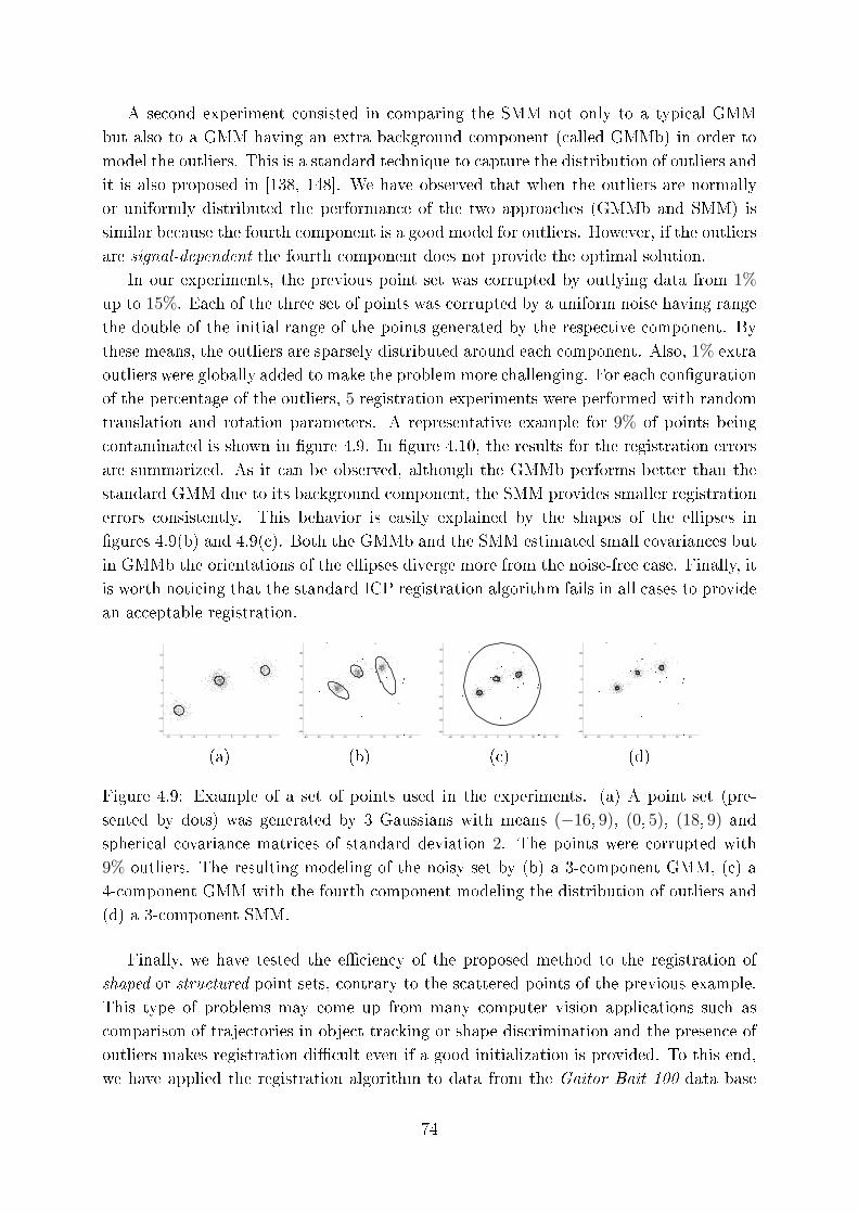
A se ond experiment onsisted in omparing the SMM not only to a typi al GMM

but also to a GMM having an extra ba kground omponent ( alled GMMb) in order to

model the outliers. This is a standard te hnique to apture the distribution of outliers and

it is also proposed in [138, 148℄. We have observed that when the outliers are normally

or uniformly distributed the performan e of the two approa hes (GMMb and SMM) is

similar be ause the fourth omponent is a good model for outliers. However, if the outliers

are signal-dependent the fourth omponent does not provide the optimal solution.

In our experiments, the previous point set was orrupted by outlying data from 1%

up to 15%. Ea h of the three set of points was orrupted by a uniform noise having range

the double of the initial range of the points generated by the respe tive omponent. By

these means, the outliers are sparsely distributed around ea h omponent. Also, 1% extra

outliers were globally added to make the problem more hallenging. For ea h on�guration

of the per entage of the outliers, 5 registration experiments were performed with random

translation and rotation parameters. A representative example for 9% of points being

ontaminated is shown in �gure 4.9. In �gure 4.10, the results for the registration errors

are summarized. As it an be observed, although the GMMb performs better than the

standard GMM due to its ba kground omponent, the SMM provides smaller registration

errors onsistently. This behavior is easily explained by the shapes of the ellipses in

�gures 4.9(b) and 4.9( ). Both the GMMb and the SMM estimated small ovarian es but

in GMMb the orientations of the ellipses diverge more from the noise-free ase. Finally, it

is worth noti ing that the standard ICP registration algorithm fails in all ases to provide

an a eptable registration.

−20 −15 −10 −5 0 5 10 15 20

−15

−10

−5

0

5

10

15

−40 −30 −20 −10 0 10 20 30 40

−40

−30

−20

−10

0

10

20

−40 −30 −20 −10 0 10 20 30 40 50

−40

−30

−20

−10

0

10

20

30

−40 −30 −20 −10 0 10 20 30 40

−40

−30

−20

−10

0

10

20

(a) (b) ( ) (d)

Figure 4.9: Example of a set of points used in the experiments. (a) A point set (pre-

sented by dots) was generated by 3 Gaussians with means (−16; 9), (0; 5), (18; 9) and

spheri al ovarian e matri es of standard deviation 2. The points were orrupted with

9% outliers. The resulting modeling of the noisy set by (b) a 3- omponent GMM, ( ) a

4- omponent GMM with the fourth omponent modeling the distribution of outliers and

(d) a 3- omponent SMM.

Finally, we have tested the eÆ ien y of the proposed method to the registration of

shaped or stru tured point sets, ontrary to the s attered points of the previous example.

This type of problems may ome up from many omputer vision appli ations su h as

omparison of traje tories in obje t tra king or shape dis rimination and the presen e of

outliers makes registration diÆ ult even if a good initialization is provided. To this end,

we have applied the registration algorithm to data from the Gaitor Bait 100 data base

74

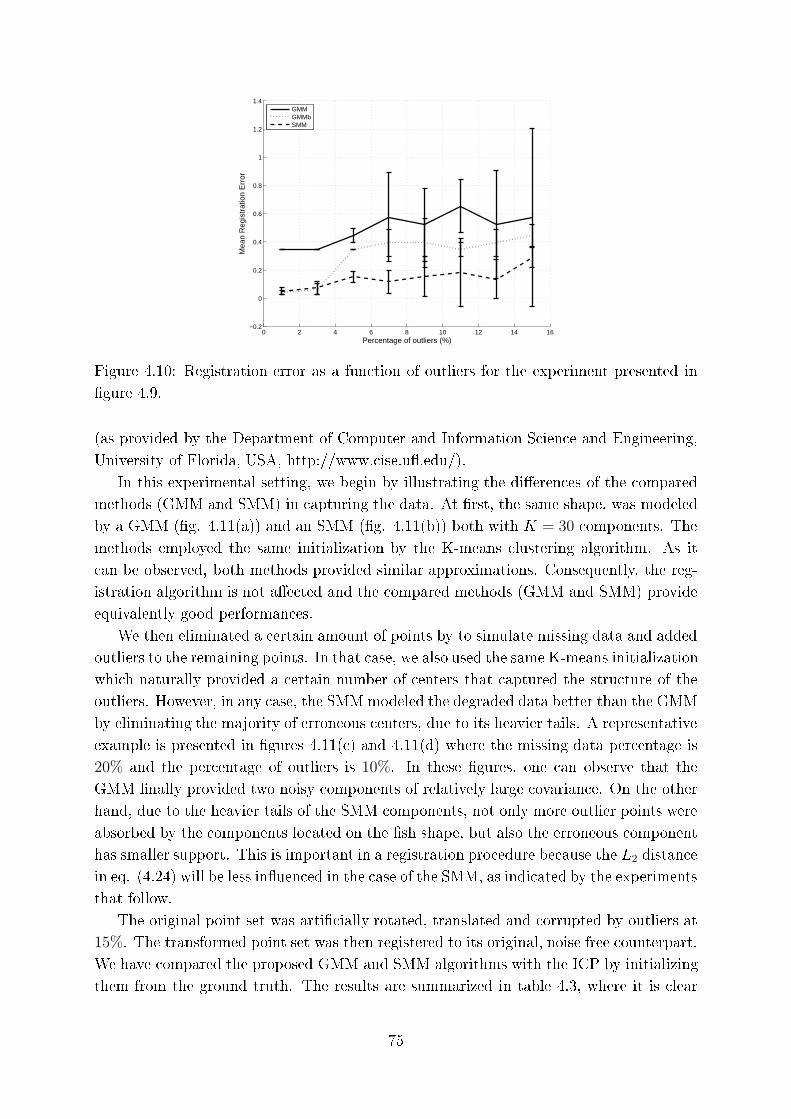
0 2 4 6 8 10 12 14 16−0.2

0

0.2

0.4

0.6

0.8

1

1.2

1.4

Percentage of outliers (%)

Mea

n R

egis

trat

ion

Err

or

GMMGMMbSMM

Figure 4.10: Registration error as a fun tion of outliers for the experiment presented in

�gure 4.9.

(as provided by the Department of Computer and Information S ien e and Engineering,

University of Florida, USA, http://www. ise.u .edu/).

In this experimental setting, we begin by illustrating the di�eren es of the ompared

methods (GMM and SMM) in apturing the data. At �rst, the same shape, was modeled

by a GMM (�g. 4.11(a)) and an SMM (�g. 4.11(b)) both with K = 30 omponents. The

methods employed the same initialization by the K-means lustering algorithm. As it

an be observed, both methods provided similar approximations. Consequently, the reg-

istration algorithm is not a�e ted and the ompared methods (GMM and SMM) provide

equivalently good performan es.

We then eliminated a ertain amount of points by to simulate missing data and added

outliers to the remaining points. In that ase, we also used the same K-means initialization

whi h naturally provided a ertain number of enters that aptured the stru ture of the

outliers. However, in any ase, the SMMmodeled the degraded data better than the GMM

by eliminating the majority of erroneous enters, due to its heavier tails. A representative

example is presented in �gures 4.11( ) and 4.11(d) where the missing data per entage is

20% and the per entage of outliers is 10%. In these �gures, one an observe that the

GMM �nally provided two noisy omponents of relatively large ovarian e. On the other

hand, due to the heavier tails of the SMM omponents, not only more outlier points were

absorbed by the omponents lo ated on the �sh shape, but also the erroneous omponent

has smaller support. This is important in a registration pro edure be ause the L2 distan e

in eq. (4.24) will be less in uen ed in the ase of the SMM, as indi ated by the experiments

that follow.

The original point set was arti� ially rotated, translated and orrupted by outliers at

15%. The transformed point set was then registered to its original, noise free ounterpart.

We have ompared the proposed GMM and SMM algorithms with the ICP by initializing

them from the ground truth. The results are summarized in table 4.3, where it is lear

75

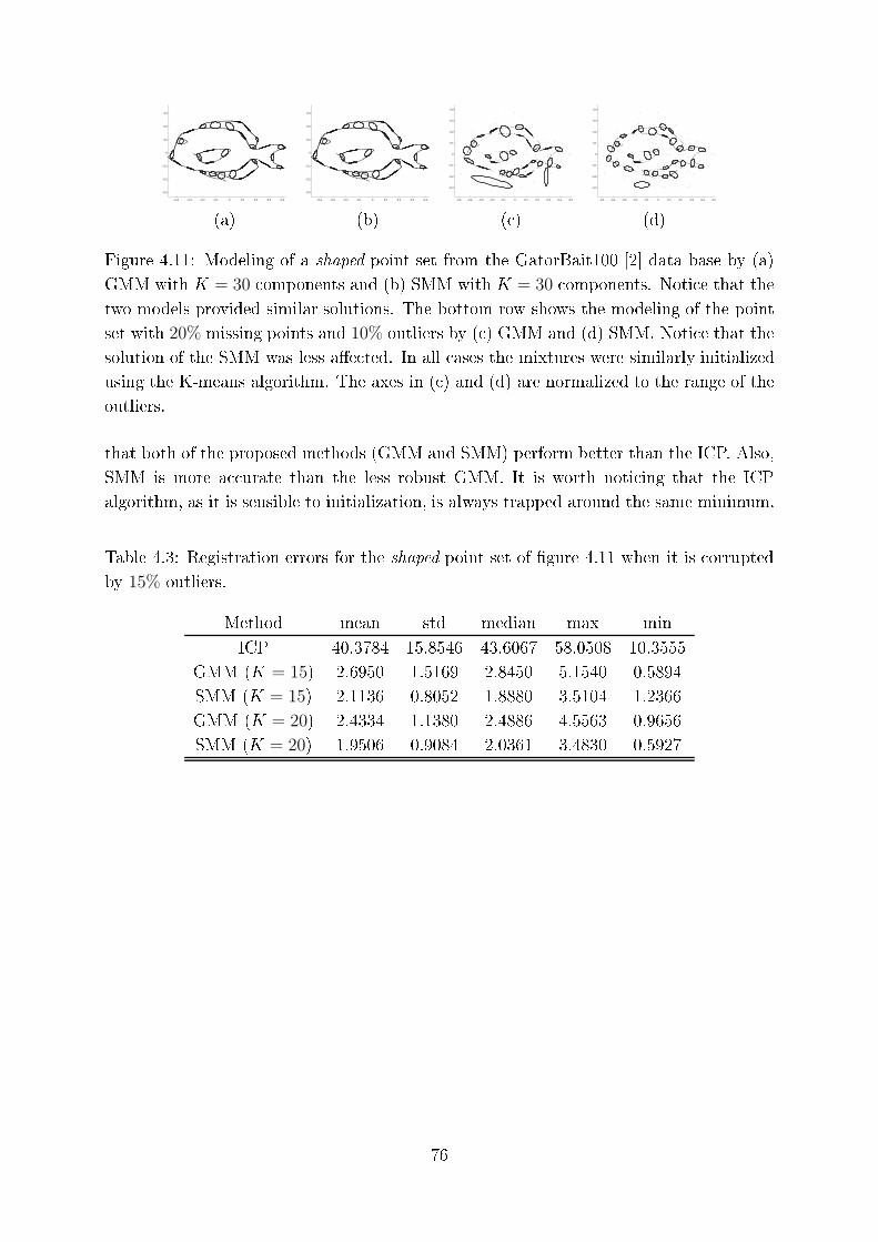
−0.4 −0.3 −0.2 −0.1 0 0.1 0.2 0.3 0.4

−0.3

−0.2

−0.1

0

0.1

0.2

0.3

−0.4 −0.3 −0.2 −0.1 0 0.1 0.2 0.3 0.4

−0.3

−0.2

−0.1

0

0.1

0.2

0.3

−0.5 −0.4 −0.3 −0.2 −0.1 0 0.1 0.2 0.3 0.4 0.5

−0.3

−0.2

−0.1

0

0.1

0.2

0.3

0.4

−0.5 −0.4 −0.3 −0.2 −0.1 0 0.1 0.2 0.3 0.4 0.5

−0.3

−0.2

−0.1

0

0.1

0.2

0.3

0.4

(a) (b) ( ) (d)

Figure 4.11: Modeling of a shaped point set from the GatorBait100 [2℄ data base by (a)

GMM with K = 30 omponents and (b) SMM with K = 30 omponents. Noti e that the

two models provided similar solutions. The bottom row shows the modeling of the point

set with 20% missing points and 10% outliers by ( ) GMM and (d) SMM. Noti e that the

solution of the SMM was less a�e ted. In all ases the mixtures were similarly initialized

using the K-means algorithm. The axes in ( ) and (d) are normalized to the range of the

outliers.

that both of the proposed methods (GMM and SMM) perform better than the ICP. Also,

SMM is more a urate than the less robust GMM. It is worth noti ing that the ICP

algorithm, as it is sensible to initialization, is always trapped around the same minimum.

Table 4.3: Registration errors for the shaped point set of �gure 4.11 when it is orrupted

by 15% outliers.

Method mean std median max min

ICP 40.3784 15.8546 43.6067 58.0508 10.3555

GMM (K = 15) 2.6950 1.5169 2.8450 5.1540 0.5894

SMM (K = 15) 2.1136 0.8052 1.8880 3.5104 1.2366

GMM (K = 20) 2.4334 1.1380 2.4886 4.5563 0.9656

SMM (K = 20) 1.9506 0.9084 2.0361 3.4830 0.5927

76

Chapter 5

Epilogue

5.1 Con lusions

5.2 Future work

5.1 Con lusions

The obje tive of this thesis was twofold: to introdu e a method for extra ting features

from images and sets of points for further analysis and to present a framework for solving

the image and point set registration problem.

As far as the feature extra tion is on erned, we fo used on modeling data with line

segments. We were motivated by the fa t that line segments show simpli ity and at the

same time they an be ombined into groups to model more ompli ated stru tures. The

pioneering work of Hough Transform has been the basis for the development of many

variants on the literature. A major problem of this lass of methods is that they assume

the number of lines as a prerequisite. Thus, the result is highly related to the tuning

of the algorithm. Moreover, they are prone to erroneous dete tions. This observation,

motivated us to propose a framework that ta kles that problem by estimating the number

of underlying line segments. Our method relies on two observations: i) the ovarian e

matrix of the points belonging to a line segment produ es an ellipse that is highly e -

entri , in fa t the linearity of the points is modeled by the minimum eigenvalue of the

orresponding ovarian e matrix and ii) the points that belong to a line segment should

follow a uniform distribution, whi h is explained by the fa t that the distan e between

su essive points is small. Eventually, those observations are quantifying some remarks

of the Gestalt theory for human per eption regarding linear stru tures. The proposed

algorithm was des ribed in hapter 1.

Considering line segments as informative features of an image or a set of points, some

appli ations are then demonstrated based on the dete ted line segments. Chapter 2 is

dedi ated to explain those appli ations.

In the beginning we dealt with a basi problem of autonomous navigation, naming the

dete tion of the vanishing point of a real s ene. A lot of methods have been proposed for

solving that problem. The most ommon work ow is to extra t the edges of an image

with an edge dete tor - most often the Canny edge dete tor is used - �t lines and then

ompute the ommon interse tion point. This approa h it is widely used. However,

we noted that it demands a pre ise tuning of the line dete tion algorithm. A basi

obje tive in this work was to preserve the simpli ity of the work ow. Sin e an eÆ ient

line segment dete tion was introdu ed in a previous hapter, we fo used on the ommon

interse tion point estimation pro ess. Thus, an eÆ ient voting s heme was established

based on distributions that model a grid laying onto the image plane and olle ts votes.

An important advantage of this approa h is that it enables the establishment of a losed

form solution. The omplete development of this approa h is a matter of ongoing resear h.

A line segment is de�ned by its dire tion along with its starting/ending points, as it

establishes a framework for reprodu ing points in any desired density. This observation led

us to the development of an algorithm for eÆ ient sampling of shapes that preserves the

initial distribution of points. Sampling is a ommon prepro essing step for many methods.

In our study, we found that by adopting an eÆ ient sampling method we managed to

improve already proposed algorithms, related to shape retrieval. The sampling s heme

was further developed and embedded in a shape re onstru tion algorithm that enables

the eÆ ient ompression of information with minimal loss.

Line segments are ideal for modeling tree stru tures like the retinal fundus image, sin e

they permit to lo ate interse tions that may be explained as bifur ations and jun tions. A

related algorithmwas presented by de�ning a neighboring riterion based on the Eu lidean

distan e.

Finally, a method for eliminating outliers was des ribed. The algorithm is based on the

Helmholtz prin iple regarding human per eption and states that in a random generated

image the expe tation of observing a stru ture should be low, ideally zero. In this ase,

line segments serve as models of underlying stru tures that may appear and assist the

omputation of the orresponding probability of a line segment. The prin iple idea is that

long line segments should be rare. A Pareto distribution was used to model the probability

fun tion of the random variable that des ribes the length of a line segment. The method

was tested both in terms of shape extra tion from heavily degraded point louds and line

�tting in a set were a large amount of outliers were present. Our method proved to be

robust and eÆ ient ompared to other state-of-the-art and widely used methods.

The se ond part of this dissertation fo used on image and point set registration. A

framework that models the registration transformation was introdu ed. A Bayesian re-

gression framework, namely the Relevan e Ve tor Ma hines, was used to des ribe a non-

rigid transformation. The basi hara teristi of this approa h is that it manages to

78

handle false-mat hes without ompromising the eÆ ien y of the model, ompared to the

ommonly used thin plate splines. Moreover, our method provides a losed form solution

for the transformation that may be used for post omputations.

The thesis on ludes with the des ription of a method for solving the rigid image and

point set registration problem, employing mixture models. By modeling the intensity dis-

tribution of the observed and the referen e image/point set and measuring their distan e

under a rigid transformation, we ompute a quantity that is minimized with respe t to

the transformation's parameters. The advantage of the method is that it an handle multi

modal images providing simultaneously eÆ ient results, ompared to the state of the art

methods.

5.2 Future Work

The output of this thesis may be the basis for further resear h, espe ially in the �eld

of the analysis of sets of s attered points. The following topi s are of interest for more

detailed investigation:

• The Helmholtz prin iple may be adopted to eliminate the need of split/merge thresh-

olds. The Helmholtz prin iple states that no per eption should be produ ed on an

image of noise. In other words, if we onsider the input set of points as a random

distribution of noise, then line segments should be less possible to be dete ted. Thus,

by de�ning a model to ompute the likelihood of an observed linear stru ture, we

may de lare this observation as valid if the orresponding probability is two small.

This approa h di�ers from the method introdu ed in [40, 41, 42℄ as it is more general

and does not assumes the existen e of a grid, as is the ase for images.

• The development of a lo al area des riptor based on the line segments that an

be used either for image/point set registration or mat hing. Line segments an be

des ribed by their start/end points, their length and dire tion. Relying on those

features, we an produ e a des riptor of the lo al neighborhood of the line segment

and then employ it to ompute the similarity between two line segments. If the line

segments are asso iated with image edges, then their similarity metri is equal to

the similarity of the orresponding image area that provided the edges. In [150℄, a

line des riptor, that follows this rationale is introdu ed.

• The use of Kalman �lters [151℄ to redu e the distortion of the proposed binary image

ompression framework based on the DSaM algorithm.

• The use of DSaM to dete t more omplex stru tures. For instan e, line segments

ould be grouped based on the lo al urvature so as to extra t more meaningful

stru tures, su h as traÆ signs.

• The use of DSaM and the retinal fundus image annotation riteria to produ e a

79

graph that des ribes ra ks on pavements and then extra t graph based features to

lassify them.

• The use of DSaM as a prepro essing step for extra ting line segments for ve torizing

raster images, like the line drawings mentioned in [152℄.

80

Bibliography

[1℄ Dataset: MPEG-7. ollege of s ien e and te hnology, temple university. (2002)

[2℄ Dataset: GatorBait 100, University of Florida (2008)

[3℄ Sebastian, T.B., Klein, P.N., Kimia, B.B.: Re ognition of shapes by editing their

sho k graphs. IEEE Transa tions on Pattern Analysis and Ma hine Intelligen e 26

(2004) 550{571

[4℄ Ferrari, V., Tuytelaars, T., Gool, L.V.: Obje t dete tion by ontour segment net-

works. In: European Conferen e on Computer Vision. (2006) 14{28

[5℄ Kovesi, P.D.: Matlab and O tave fun tions for vomputer vision and image pro ess-

ing (2009)

[6℄ Gerogiannis, D., Nikou, C., Likas, A.: Modeling sets of unordered points using

highly e entri ellipses. EURASIP Journal on Advan es in Signal Pro essing (2014)

[7℄ Belongie, S., Malik, J., Puzi ha, J.: Shape mat hing and obje t re ognition using

Shape Contexts. IEEE Transa tions on Pattern Analysis and Ma hine Intelligen e

24 (2002) 1{19

[8℄ Medioni, G., Lee, M.S., Tang, C.K.: A Computational Framework for Segmentation

and Grouping. Elsevier (2000)

[9℄ P. Mordohai and G. G. Medioni: Tensor Voting. A Per eptual Organization Ap-

proa h to Computer Vision and Ma hine Learning. Morgan and Claypool (2007)

[10℄ Ramer, U.: An iterative pro edure for the polygonal approximation of plane urves.

Computer Graphi s and Image Pro essing (1972) 244{256

[11℄ O'Connell, K.J.: Obje t-adaptive vertex-based shape oding method. IEEE Trans-

a tions on Cir uits and Systems for Video Te hnology 7 (1997) 251{255

[12℄ Xiao hao, W., Xiuping, L., Hong, Q.: Robust surfa e onsolidation of s anned

thi k point louds. In: International Conferen e on Computer-Aided Design and

Computer Graphi s. (2013) 38{43

81

[13℄ Ester, M., Kriegel, H.P., J�org, S., Xiaowei, X.: A density-based algorithm for dis-

overing lusters in large spatial databases with noise. In: International Conferen e

on Knowledge Dis overy and Data Mining, AAAI Press (1996) 226{231

[14℄ Chui, H., Rangarajan, A.: A new algorithm for non-rigid point mat hing. In:

IEEE Computer So iety Conferen e on Computer Vision and Pattern Re ognition.

Volume 2. (2000) 40{51

[15℄ Bookstein, F.L.: Prin ipal Warps: Thin-Plate Spilnes and the de omposition of

deformations. IEEE Transa tions on Pattern Analysis and Ma hine Intelligen e 11

(1989) 567{585

[16℄ Tsin, Y., Kanade, T.: A orrelation-based approa h to robust point set registration.

In: European Conferen e on Computer Vision. (2004) 558{569

[17℄ Myronenko, A., Song, X.: Point set registration: Coherent Point Drift. IEEE

Transa tions on Pattern Analysis and Ma hine Intelligen e 32 (2010) 2262{2275

[18℄ Cantoni, V., Lombardi, L., Porta, M., Si ard, N.: Vanishing point dete tion: repre-

sentation analysis and new approa hes. In: 11th International Conferen e on Image

Analysis and Pro essing. (2001) 90{94

[19℄ Dori, D., Wenyin, L.: Sparse pixel ve torization: An algorithm and its performan e

evaluation. IEEE Transa tions on Pattern Analysis and Ma hine Intelligen e 21

(1999) 202{215

[20℄ Se, S., Brady, M.: Road feature dete tion and estimation. Ma hine Vision and

Appli ations 14 (2003) 157{165

[21℄ Kolesnikov, A.: ISE-bounded polygonal approximation of digital urves. Pattern

Re ognition Letters 33 (2012) 1329{1337

[22℄ Illingworth, J., Kittler, J.: A survey of the Hough Transform. Computer Vision,

Graphi s, and Image Pro essing 44 (1988) 87{116

[23℄ Leavers, V.F.: Whi h Hough Transform? Computer Vision, Graphi s and Image

Pro essing: Image Understanding 58 (1993) 250{264

[24℄ Xu, L., Oja, E., Kultanen, P.: A new urve dete tion method: Randomized Hough

Transform (RHT). Pattern Re ognition Letters (1990) 331{338

[25℄ M Laughlin, R.A.: Randomized Hough Transform: Improved ellipse dete tion with

omparison. Pattern Re ognition Letters 19 (1998) 299{305

[26℄ Kiryati, N., Eldar, Y., Bru kstein, A.M.: A probabilisti Hough Transform. Pattern

Re ognition 24 (1991) 303{316

82

[27℄ Matas, J., Galambos, C., Kittler, J.: Progressive probabilisti Hough Transform.

In: British Ma hine Vision Conferen e. Volume I., London, UK (1998) 256{265

[28℄ Chung, K., Lin, Z., Huang, S., Huang, Y., Liao, H.M.: New orientation-based

elimination approa h for a urate line-dete tion. Pattern Re ognition Letters 31

(2010) 11{19

[29℄ Chatzis, V., Pitas, I.: Fuzzy ell Hough Transform for urve dete tion. Pattern

Re ognition 30 (1997) 2031{2042

[30℄ K�alvi�ainen, H., Hirvonen, P., Xu, L., Oja, E.: Probabilisti and non-probabilisti

Hough transforms: overview and omparisons. Image and Vision Computing 13

(1995) 239{252

[31℄ Atiquzzaman, M., Akhtar, M.W.: A robust Hough Transform te hnique for om-

plete line segment des ription. Real Time Imaging (1995) 419{426

[32℄ Chau, C., Siu, W.: Adaptive dual-point Hough Transform for obje t re ognition.

Computer Vision and Image Understanding 96 (2004) 1{16

[33℄ Cheng, H.D., Guo, Y., Zhang, Y.: A novel Hough Transform based on eliminating

parti le swarm optimization and its appli ations. Pattern Re ognition 42 (2009)

1959{1969

[34℄ Moore, G.A.: Automati s anning and omputer pro ess for the quantitative anal-

ysis of mi rographs and equivalent subje ts. Pi torial Pattern Re ognition (1968)

275{362

[35℄ Li, C., Wang, Z., Li, L.: An improved Hough Transform algorithm on straight line

dete tion based on Freeman hain ode. In: 2nd International Congress on Image

and Signal Pro essing. (2009) 1{4

[36℄ Martin, F., Robert, B.: Random sample onsensus: a paradigm for model �tting

with appli ations to image analysis and automated artography. Communi ations

of the ACM 24 (1981) 381{385

[37℄ Bhowmi k, P., Bhatta harya, B.: Fast polygonal approximation of digital urves

using relaxed straightness properties. IEEE Transa tions on Pattern Analysis and

Ma hine Intelligen e 29 (2007) 1590{1602

[38℄ Leite, J., Han o k, E.: Iterative urve organisation with the EM algorithm. Pattern

Re ognition Letters 18 (1997) 143{155

[39℄ Desolneux, A., Moisan, L., Morel, J.M.: Meaningful allignments. International

Journal of Computer Vision 40 (2000) 7{23

83

[40℄ von Gioi, R.G., Jakubowi z, J., Morel, J.M., Randall, G.: On straight line segment

dete tion. Journal of Mathemati al Imaging and Vision 32 (2008) 313{347

[41℄ von Gioi, R.G., Jakubowi z, J., Morel, J.M., Randall, G.: LSD: A fast line segment

dete tor with a false dete tion ontrol. IEEE Transa tions on Pattern Analysis and


[42℄ von Gioi, R.G., Jakubowi z, J., Morel, J.M., Randall, G.: LSD: A line segment

dete tor. Image Pro essing On Line 2 (2012) 35{55

[43℄ Marr, D.: Vision. Freeman Publishers, New York (1982)

[44℄ Canny, J.: A omputational approa h to edge dete tion. IEEE Transa tions on

Pattern Analysis and Ma hine Intelligen e 8 (1986) 679{698

[45℄ Bishop, C.M.: Pattern re ognition and ma hine learning. Springer, Dordre ht, The

Netherlands (2006)

[46℄ Matas, J., Galambos, C., Kittler, J.: Robust dete tion of lines using the progressive

probabilisti Hough Transform. Computer Vision and Image Understanding 78

(April 2001) 119{137

[47℄ Bradski, G., Kaehler, A.: Learning OpenCV: Computer Vision with the OpenCV.

O'Reilly Media, Sebastoupol, California (2008)

[48℄ Coughlin, J.M., Yuille, A.: Manhattan world: ompass dire tion from a single

image by Bayesian inferen e. In: IEEE International Conferen e on Computer

Vision. Volume 2. (1999) 941{947

[49℄ Denis, P., Elder, .H., Estrada, F.J.: EÆ ient edge-based methods for estimating

Manhattan frames in urban imagery. In: European Conferen e on Computer Vision

ECCV. Volume 2. (2008) 107{210

[50℄ Almansa, A., Desolneux, A., Vame h, S.: Vanishing point dete tion without any a

priori information. IEEE Transa tions on Pattern Analysis and Ma hine Intelligen e

25 (2003) 502 { 507

[51℄ Kose ka, J., Zhang, W.: Video ompass. In: European Conferen e on Computer

Vision. (2002) 476{491

[52℄ Tardif, J.P.: Non-iterative approa h for fast and a urate vanishing point dete tion.

In: IEEE International Conferen e on Computer Vision, Kyoto, Japan (September

27 - O tober 4, 2009) 1250{1257

[53℄ Rother, C.: A new approa h to vanishing point dete tion in ar hite tural environ-

ments. Image and Vision Computing 20 (2002) 647{655

84

[54℄ Li, B., Peng, K., Ying, X., Zha, H.: Vanishing point dete tion using as aded 1d

Hough Transform from single images. Patter Re ognition Letters 33 (2012) 1{8

[55℄ Martin, D., Fowlkes, C., Tal, D., Malik, J.: A database of human segmented natu-

ral images and its appli ation to evaluating segmentation algorithms and measuring

e ologi al statisti s. In: IEEE International Conferen e one Computer Vision. Vol-

ume 2. (2001) 416{423

[56℄ Alivanoglou, A., Likas, A.: Probabilisti models based on the Pi-Sigmoid distribu-

tion. In: 3rd IAPR Workshop on Arti� ial Neural Networks in Pattern Re ognition.

(2008) 36{43

[57℄ University, B.: Mat hing with Shape Contexts (2002)

[58℄ Moenning, C., Dodgson, N.A.: Fast mar hing farthest point sampling. In: EURO-

GRAPHICS. (2003)

[59℄ Bronstein, A., Bronstein, M., Bronstein, M., Kimmel, R.: Numeri al geometry of

non-rigid shapes. Springer-Verlag New York In (2008)

[60℄ Chen, J.J., Chiang, C.C., Lin, D.W.: A generalized 3d shape sampling method

and �le format for storage or indexing. In: International Conferen e on Image

Pro essing. Volume 2. (2000) 780{783

[61℄ Osada, R., Funkhouser, T., Chazelle, B., Dobkin, D.: Shape distributions. ACM

Transa tions on Graphi s 21 (2002) 807{832

[62℄ Wang, J., Bai, X., You, X., Liu, W., Late ki, J.: Shape mat hing and lassi� ation

using height fun tions. Pattern Re ognition Letters 33 (2012) 134{143

[63℄ Azariadis, P.N., Sapidis, N.S.: Drawing urves onto a loud of points for point-based

modelling. Computer-Aided Design 37 (2005) 109{122

[64℄ Roweis, S.T., Saul, L.K.: Nonlinear dimensionality redu tion by lo ally linear

embedding. S ien e 290 (2000) 2323{2326

[65℄ Std., I.I.: Information te hnology { oding of audio-visual obje ts { part 2: Visual

oding. http://www.digitalpreservation.gov/formats/fdd/fdd000080.shtmln (1999)

A essed on January, 2015.

[66℄ Freeman, H.: Computer pro essing of line-drawing images. ACM Comput. Surv. 6

(1974) 57{97

[67℄ Katsaggelos, A.K., Kondi, L.P., Meier, F.W., Ostermann, J., S huster, G.M.:

MPEG-4 and rate-distortion-based shape- oding te hniques. Pro eedings of the

IEEE 86 (1998) 1126{1154

85

[68℄ Aghito, S.M., For hhammer, S.: Context-based oding of bilevel images enhan ed

by digital straight line analysis. IEEE Transa tions on Image Pro essing 15 (2006)

2120{2130

[69℄ Klette, R., Rosenfeld, A.: Digital straightness - a review. Dis rete Applied Mathe-

mati s 139 (2004) 197{230

[70℄ 11544, I.I.S.: Coded representension of pi ture and audio information - progressive

bi-level image ompression (1993)

[71℄ 14492, I.I.S.: Coded representension of pi ture and audio information - lossy/lossless

oding of bi-level images (JBIG2) (2000)

[72℄ Aghito, S.M., For hhammer, S.: EÆ ient oding of shape and transparen y for

video obje ts. IEEE Transa tions on Image Pro essing 16 (2007) 2234{2244

[73℄ San hez-Cruz, H.: Proposing a new ode by onsidering pie es of dis rete straight

lines in ontour shapes. Journal of Visual Communi ation and Image Representation

21 (2010) 311{324

[74℄ Akimov, A., Kolesnikov, A., Fr�anti, P.: Lossless ompression of map ontours by

ontext tree modeling of hain odes. Pattern Re ognition 40 (2007) 944{952

[75℄ Pinho, A.J.: A JBIG-based approa h to the en oding of ontour maps. IEEE

Transa tions on Image Pro essing 9 (2000) 936{941

[76℄ Bresenham, J.E.: Algorithm for omputer ontrol of a digital plotter. IBM Systems

Journal 4 (1965) 25{30

[77℄ ITU-T: T.6: Fa simile oding s hemes and oding ontrol fun tions for group

4 fa simile apparatus. http://www.itu.int/re /T-REC-T.6/en (1984) A essed on

January, 2015.

[78℄ Wang, H., S huster, G.M., Katsaggelos, A.K., Pappas, T.N.: An eÆ ient rate-

distortion optimal shape oding approa h utilizing a skeleton-based de omposition.

IEEE Transa tions on Image Pro essing 12 (2003) 1181{1193

[79℄ Ausbe k, J.P.J.: The pie ewise- onstant image model. IEEE Pro eedings (2000)

1779{1789

[80℄ : Djvu libre (2015)

[81℄ Patton, N., Aslam, T.M., Ma Gillivray, T., Dearye, I.J., Dhillonb, B., Eikelboomf,

R.H., Yogesana, K., Constablea, I.J.: Retinal image analysis: Con epts, appli a-

tions and potential. Progress in Retinal and Eye Resear h 25 (2006) 99{127

86

[82℄ Azzopardi, G., Petkov, N.: Dete tion of retinal vas ular bifur ations by trainable

V4-like �lters. In: 14th International Conferen e on Computer Analysis of Images

and Patterns, Spain (2011) 451{459

[83℄ Staal, J., Abramo�, M., Niemeijer, M., Viergever, M., van Ginneken, B.: Ridge

based vessel segmentation in olor images of the retina. IEEE Transa tions on

Medi al Imaging 23 (2004) 501{509

[84℄ Azzopardi, G., Petkov, N.: Retinal fundus images - Ground truth of vas ular

bifur ations and rossovers (2011)

[85℄ Lemaitre, C., Perdo h, M., Rahmoune, A., Matas, J., Miteran, J.: Dete tion and

mat hing of urvilinear stru tures. Pattern Re ognition 44 (2011) 1514{1527

[86℄ Sofka, M., Stewart, C.V.: Retinal vessel extra tion using multis ale mat hed �lters,

on�den e and edge measures. IEEE Transa tions on Medi al Imaging 25 (2006)

1531{1546

[87℄ Gonzalez, R.C., Woods, R.E.: Digital image pro essing, 3rd edition. Prenti e Hall,

Upper Saddle River, New Jersey (2008)

[88℄ C. C. Aggarwal: Outlier Analysis. Springer (2013)

[89℄ Thompson, R.: A note on restri ted maximum likelihood estimation with an alter-

native outlier model. Journal of the Royal Statisti al So iety 47 (1985) 53{55

[90℄ Rusu, R.B., Cousins, S.: 3d is here: Point loud library (PCL). In: IEEE Interna-

tional Conferen e on Roboti s and Automation, Shanghai, China (2011)

[91℄ S hall, O., Belyaev, A., Seidel, H.P.: Robust �ltering of noisy s attered point data.

In: Eurographi s Symposium on Point-Based Graphi s. (2005) 71{77

[92℄ Weyri h, T., Pauly, M., Keiser, R., Heinzle1, S., S andella, S., Gross1, M.: Post-

pro essing of s anned 3d surfa e data. In: Eurographi s Symposium on Point-Based

Graphi s. (2004) 85{94

[93℄ Ert�oz, L., Steinba h, M., Kumar, V.: Finding lusters of di�erent sizes, shapes, and

densities in noisy, high dimensional data. In: 2nd SIAM International Conferen e

on Data Mining. (2003)

[94℄ Xie, H., M Donnell, K.T., Hong, Q.: Surfa e re onstru tion of noisy and defe tive

data sets. In: IEEE Visualization. (2004) 259{266

[95℄ Desolneux, A., Moisan, L., Morel, J.M.: Gestalt theory and omputer vision. In:

Seeing, Thinking and Knowing. Volume 38. Kluwer A ademi Publishers (2004)

71{101

87

[96℄ Desolneux, A., Moisan, L., Morel, J.M.: Edge dete tion by Helmholtz prin iple.

Journal of Mathemati al Imaging and Vision 14 (2001) 271{284

[97℄ Desolneux, A., Moisan, L., Morel, J.M.: From Gestalt Theory to Image Analysis:

a Probabilisti Approa h. Springer (2008)

[98℄ Arnold, B.C.: Pareto distributions. Statisti al distributions in s ienti� work series.

International Co-operative Publishing House (1983)

[99℄ Dumou hel, W., O'Brien, F.: Integrating a robust option into a multiple regression

omputing environment. In: Computing and Graphi s in Statisti s. Springer-Verlag

New York, In . (1991) 41{48

[100℄ Besl, P.J., M Kay, N.D.: A method for registration of 3d shapes. IEEE Transa tions

on Pattern Analysis and Ma hine Intelligen e 14 (1992) 239{256

[101℄ Rusinkiewi z, S., Levoy, M.: EÆ ient variants of the ICP algorithm. In: The 3rd

International Conferen e on 3D Digital Imaging and Modeling. (2001)

[102℄ Gold, S., Lu, C.P., Rangarajan, A., Pappu, S., Mjolsness, E.: New algorithms for

2d and 3d point mat hing: Pose estimation and orresponden e. In Tesauro, G.,

Touretzky, D., Leen, T., eds.: Advan es in Neural Information Pro essing Systems.

Volume 7., The MIT Press (1995) 957{964

[103℄ Jian, B., Vemuri, B.C.: Robust point set registration using Gaussian mixture

models. IEEE Transa tions on Pattern Analysis and Ma hine Intelligen e 33 (2011)

1633{1645

[104℄ Gerogiannis, D., Nikou, C., Likas, A.: The mixtures of Student's t-distributions as

a robust framework for rigid registration. Image and Vision Computing 27 (2009)

1285{1294

[105℄ Tu, Z., Zheng, S., Yuille, A.: Shape mat hing and registration by data-driven EM.

Computer Vision and Image Understanding 109 (2008) 290{304

[106℄ Suk, T., Flusser, J.: Point-based proje tive invariants. Pattern Re ognition 33

(2000) 251{261

[107℄ Caetano, T.S., Caelli, T., S huurmans, D., Barone, D.A.C.: Graphi al models

and point pattern mat hing. IEEE Transa tions on Pattern Analysis and Ma hine

Intelligen e 28 (2006) 1646{1663

[108℄ Zheng, Y., Doermann, D.S.: Robust point mat hing for non-rigid shapes by pre-

serving lo al neighborhood stru tures. IEEE Transa tions on Pattern Analysis and


88

[109℄ Tipping, M.E.: Sparse Bayesian learning and the relevan e ve tor ma hine. Journal

of Ma hine Learning Resear h 1 (2001) 211{244

[110℄ Tan, L., Fyfe, C.: Canoni al orrelation analysis - a relevan e ve tor approa h. In:

The 9th European Symposium on Arti� ial Neural Networks. (2001)

[111℄ Iwai, Y., Cipolla, R.: Multivariate sparse Bayesian regression and its appli ation

for fa ial feature dete tion. In: IAPR Conferen e on Ma hine Vision Appli ations.

(2005)

[112℄ Chui, H., Rangarajan, A.: A new point mat hing algorithm for non-rigid registra-

tion. Computer Vision and Image Understanding 89 (2003) 114{141

[113℄ Papadimitriou, C.H., Steiglitz, K.: Combinatorial optimization. Algorithms and

omplexity. Dover (1998)

[114℄ Dempster, P., Laird, N.M., Rubin, D.B.: Maximum likelihood from in omplete

data via the EM algorithm. Journal of the Royal Statisti al So iety 39 (1977) 1{38

[115℄ Tipping, M.: Matlab ode for univariate RVM implementation (2006)

[116℄ Zitova, B., Flusser, J.: Image registration methods: a survey. Image and Vision

Computing 21 (2003) 1{36

[117℄ Maintz, J.B.A., Viergever, M.A.: A survey of medi al image registration te hniques.

Medi al Image Analysis 2 (1998) 1{36

[118℄ Bankman, I.: Handbook of medi al image pro essing and analysis. A ademi Press

(2000)

[119℄ Hajnal, J.V., Hill, D.L.G., Hawkes, D.J.: Medi al image registration. CRC Press

(2001)

[120℄ Nikou, C., Heitz, F., Armspa h, J.P.: Robust voxel similarity metri s for the

registration of dissimilar single and multimodal images. Pattern Re ognition 32

(1999) 1351{1368

[121℄ Jensen, J.R.: Introdu tory digital image pro essing: a remote sensing perspe tive.

3rd edn. Prenti e Hall (2004)

[122℄ Heitz, F., Ma�tre, H., de Couessin, C.: Event dete tion in multisour e imaging:

appli ation to �ne arts painting analysis. IEEE Transa tions on A ousti , Spee h

and Signal Pro essing 38 (1990) 695{704

[123℄ Viola, P., W. Wells III: Alignment by maximization of mutual information. Inter-

national Journal of Computer Vision 24 (1997) 137{154

89

[124℄ Maes, F., Collignon, A., Vandermeulen, D., Mar hal, G., Suetens, P.: Multimodality

image registration by maximization of mutual information. IEEE Transa tions on

Medi al Imaging 16 (1997) 187{198

[125℄ Pluim, J., Maintz, J.B.A., Viergever, M.: Mutual information based registration

of medi al images: a survey. IEEE Transa tions on Medi al Imaging 22 (2004)

986{1004

[126℄ Hermosillo, G., Faugeras, O.: Dense image mat hing with global and lo al statis-

ti al riteria. In: IEEE Conferen e on Computer Vision and Pattern Re ognition.

Volume 1., Los Alamitos, USA (2001) 73{78

[127℄ Th�evenaz, P., Unser, M.: Optimization of mutual information for multiresolution

image registration. IEEE Transa tions on Image Pro essing 9 (2000) 2083{2099

[128℄ Mattes, D., Haynor, D.R., Vesselle, H., Lewellen, T.K., Eubank, W.: Nonrigid

multimodality image registration. In Hanson, K., ed.: SPIE Medi al Imaging Con-

feren e. Volume 4322., San Diego, USA (2003) 1609{1620

[129℄ Rajwade, A., Banerjee, A., Rangarajan, A.: A new method of probability density

estimation with appli ation to mutual information based image registration. In:

IEEE Conferen e on Computer Vision and Pattern Re ognition, New York, USA

(2006) 1769{1776

[130℄ M La hlan, G.: Finite mixture models. Wiley-Inters ien e (2000)

[131℄ Leventon, M., Grimson, E.: Multi-modal volume registration using joint intensity

distributions. In: Medi al Image Computing and Computer Assisted Intervention

Conferen e. (1998) 1057{1066

[132℄ Guimond, A., Ro he, A., Aya he, N., Meunier, J.: Three-dimensional multimodal

brain warping using the demons algorithm and adaptive intensity orre tions. IEEE

Transa tions on Medi al Imaging 20 (2001) 58{69

[133℄ Hellier, P.: Consistent intensity orre tion of MR images. In: IEEE International

Conferen e on Image Pro essing. Volume 1., Bar elona, Spain (2003) 1109{1112

[134℄ Jian, B., Vemuri, B.C.: A robust algorithm for point set registration using mixture

of gaussians. In: IEEE International Conferen e on Computer Vision, Beijing,

China (2005) 1246{1251

[135℄ Herbin, M., Venot, A., Devaux, J.Y., Walter, E., Lebru he , F., Dubertet, L., Rou-

ayrol, J.C.: Automated registration of dissimilar images: appli ation to medi al

imagery. Computer Vision, Graphi s and Image Pro essing 47 (1989) 77{88

90

[136℄ Ro he, A., Penne , X., Malandain, G., Aya he, N.: Rigid registration of 3d ultra-

sound with MR images: a new approa h ombining intensity and gradient informa-

tion. IEEE Transa tions on Medi al Imaging 20 (2001) 1038{1049

[137℄ Bishop, C., Svensen, M.: Robust Bayesian mixture modelling. Neuro omputing

(2005) 69{74

[138℄ Peel, D., M La hlan, G.J.: Robust mixture modeling using the t-distribution.

Statisti s and Computing 10 (2000) 339{348

[139℄ Granger, S., Penne , X.: Multi-s ale EM-ICP: A fast and robust approa h for

surfa e registration. In: European Conferen e on Computer Vision. (2002) 418{432

[140℄ Chetverikov, D., Stepanov, D., Krsek, P.: Robust Eu lidean alignment of 3d point

sets: the trimmed iterative losest point algorithm. Image and Vision Computing

23 (2004) 299{309

[141℄ Phillips, J., Liu, R., Tomasi, C.: Outlier robust ICP for minimizing RMSD. In:

The 6th International Conferen e on 3D Digital Imaging and Modeling. (2007)

[142℄ Rangarajan, A., Chui, H., Bookstein, F.L.: The softassign pro rustes mat hing

algorithm. In: The 15th International Conferen e on Information Pro essing in

Medi al Imaging. Le ture Notes in Computer S ien e. Volume 1230. (1997) 29{42

[143℄ Rangarajan, A., Chui, H., Dun an, S.: Rigid point feature registration using mutual

information. Medi al Image Analysis 4 (1999) 1{17

[144℄ Taron, M., Paragios, N., Jolly, M.: Registration with un ertainties and statisti al

modeling of shapes with variable metri kernels. IEEE Transa tions on Pattern

Analysis and Ma hine Intelligen e 31 (2009) 99{113

[145℄ Myronenko, A., Song, X., M.

�

A. Carreira-Perpi~n�an: Non-rigid point set registration:

Coherent Point Drift. In S h�olkopf, B., Platt, J., Ho�man, T., eds.: The 20th

Conferen e on Advan es in Neural Information Pro essing Systems. MIT Press,

Van ouver, Canada (2006) 1009{1016

[146℄ Wang, F., Vemuri, C.B., Rangarajan, A., S hmalfuss, M.I., Eisens henk, J.S.: Si-

multaneous non-rigid registration of multiple point sets and atlas onstru tion. In:

European Conferen e on Computer Vision. (2006) 551{563

[147℄ Fukunaga, K.: Introdu tion to statisti al pattern re ognition. A ademi Press

(1990)

[148℄ Brandt, S.S.: Maximum likelihood robust regression by mixture models. Journal of

Mathemati al Imaging and Vision 25 (2006) 25{48

91

[149℄ Pluim, J., Maintz, J.B.A., Viergever, M.: Interpolation artefa ts in mutual

information-based image registration. Computer Vision and Image Understanding

77 (2000) 211{232

[150℄ Wang, L., U. Neumann, U., You, S.: Wide-baseline image mat hing using line

signatures. In: International Conferen e on Computer Vision. (2009) 1311{1318

[151℄ Prin e, S.J.: Computer vision. Models, learning and inferen e. Cambridge Univer-

sity Press (2012)

[152℄ Hilaire, X., Tombre, K.: Robust and a urate ve torization of line drawings. IEEE

Transa tions on Pattern Analysis and Ma hine Intelligen e 28 (2006) 8901{904

[153℄ Bourgeois, F., Lassalle, J.C.: An extension of the Munkres algorithm for the as-

signment problem to re tangular matri es. Communi ations of the ACM 12 (De .

1971) 802{804

92

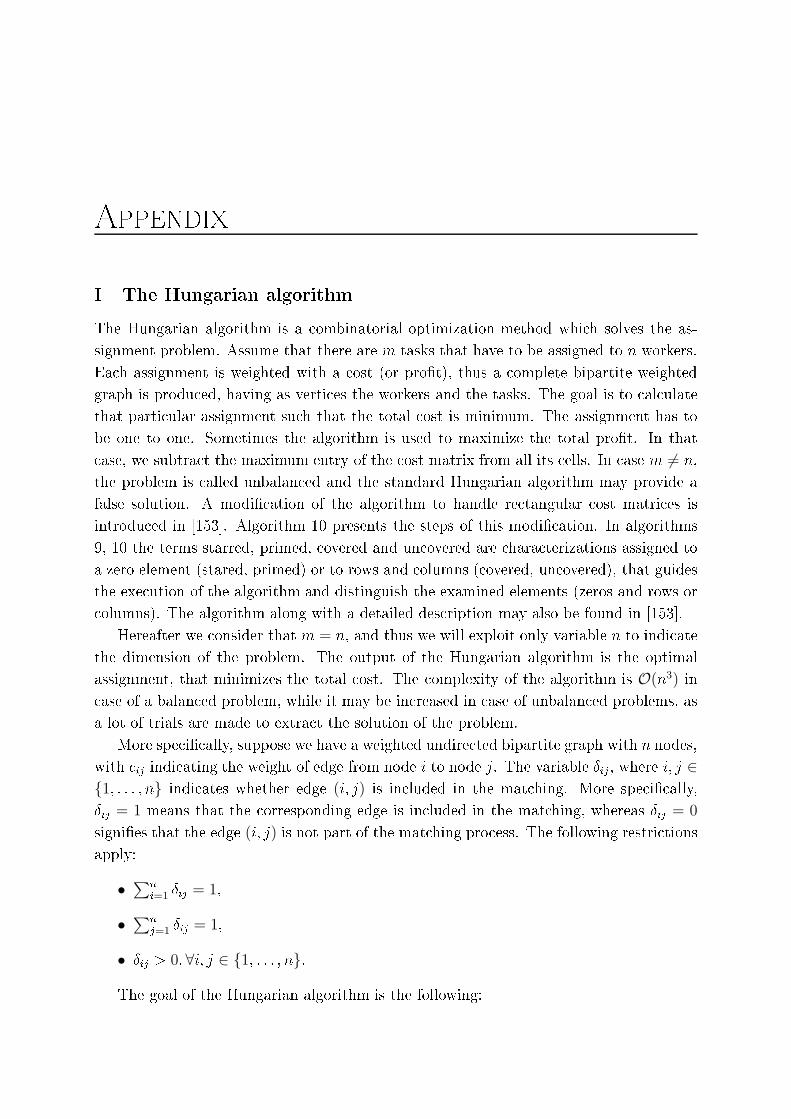
Appendix

I The Hungarian algorithm

The Hungarian algorithm is a ombinatorial optimization method whi h solves the as-

signment problem. Assume that there are m tasks that have to be assigned to n workers.

Ea h assignment is weighted with a ost (or pro�t), thus a omplete bipartite weighted

graph is produ ed, having as verti es the workers and the tasks. The goal is to al ulate

that parti ular assignment su h that the total ost is minimum. The assignment has to

be one to one. Sometimes the algorithm is used to maximize the total pro�t. In that

ase, we subtra t the maximum entry of the ost matrix from all its ells. In ase m 6= n,

the problem is alled unbalan ed and the standard Hungarian algorithm may provide a

false solution. A modi� ation of the algorithm to handle re tangular ost matri es is

introdu ed in [153℄. Algorithm 10 presents the steps of this modi� ation. In algorithms

9, 10 the terms starred, primed, overed and un overed are hara terizations assigned to

a zero element (stared, primed) or to rows and olumns ( overed, un overed), that guides

the exe ution of the algorithm and distinguish the examined elements (zeros and rows or

olumns). The algorithm along with a detailed des ription may also be found in [153℄.

Hereafter we onsider that m = n, and thus we will exploit only variable n to indi ate

the dimension of the problem. The output of the Hungarian algorithm is the optimal

assignment, that minimizes the total ost. The omplexity of the algorithm is O(n3) in

ase of a balan ed problem, while it may be in reased in ase of unbalan ed problems, as

a lot of trials are made to extra t the solution of the problem.

More spe i� ally, suppose we have a weighted undire ted bipartite graph with n nodes,

with

ij

indi ating the weight of edge from node i to node j. The variable Æ

ij

, where i; j ∈{1; : : : ; n} indi ates whether edge (i; j) is in luded in the mat hing. More spe i� ally,

Æ

ij

= 1 means that the orresponding edge is in luded in the mat hing, whereas Æ

ij

= 0

signi�es that the edge (i; j) is not part of the mat hing pro ess. The following restri tions

apply:

• ∑n

i=1 Æij = 1,

• ∑n

j=1 Æij = 1,

• Æ

ij

> 0; ∀i; j ∈ {1; : : : ; n}.

The goal of the Hungarian algorithm is the following:

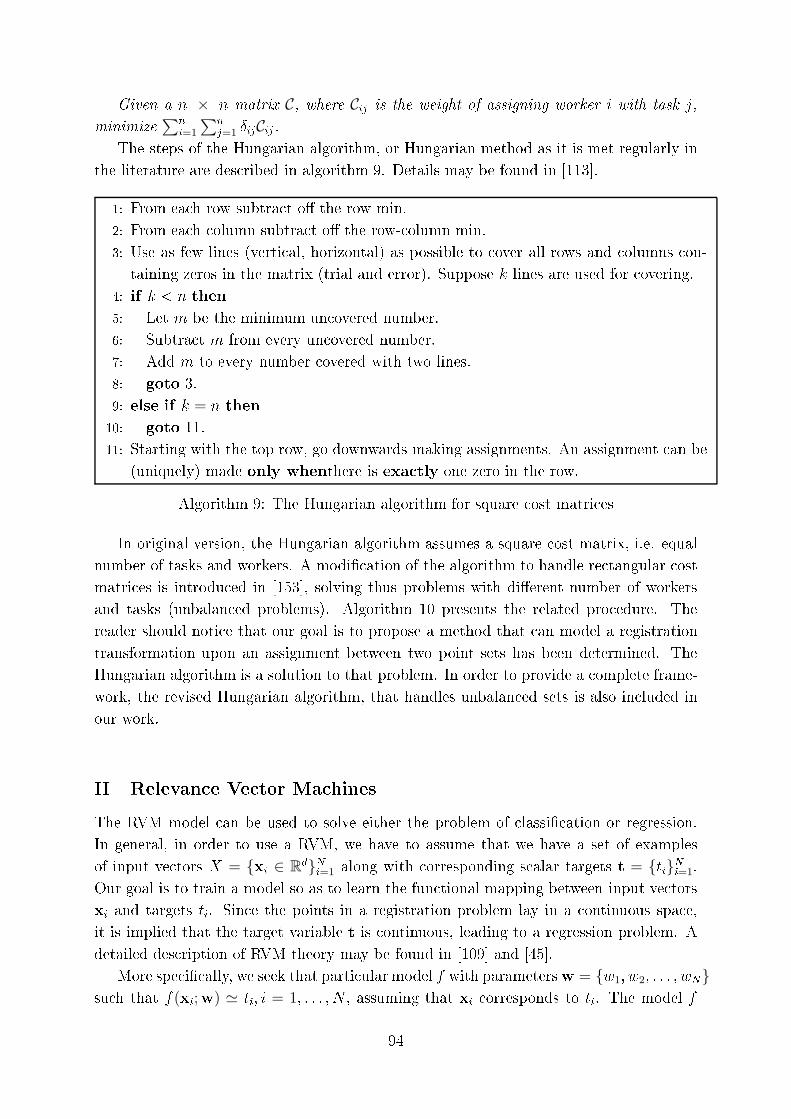
Given a n × n matrix C, where Cij

is the weight of assigning worker i with task j,

minimize

∑n

i=1

∑n

j=1 ÆijCij.The steps of the Hungarian algorithm, or Hungarian method as it is met regularly in

the literature are des ribed in algorithm 9. Details may be found in [113℄.

1: From ea h row subtra t o� the row min.

2: From ea h olumn subtra t o� the row- olumn min.

3: Use as few lines (verti al, horizontal) as possible to over all rows and olumns on-

taining zeros in the matrix (trial and error). Suppose k lines are used for overing.

4: if k < n then

5: Let m be the minimum un overed number.

6: Subtra t m from every un overed number.

7: Add m to every number overed with two lines.

8: goto 3.

9: else if k = n then

10: goto 11.

11: Starting with the top row, go downwards making assignments. An assignment an be

(uniquely) made only whenthere is exa tly one zero in the row.

Algorithm 9: The Hungarian algorithm for square ost matri es

In original version, the Hungarian algorithm assumes a square ost matrix, i.e. equal

number of tasks and workers. A modi� ation of the algorithm to handle re tangular ost

matri es is introdu ed in [153℄, solving thus problems with di�erent number of workers

and tasks (unbalan ed problems). Algorithm 10 presents the related pro edure. The

reader should noti e that our goal is to propose a method that an model a registration

transformation upon an assignment between two point sets has been determined. The

Hungarian algorithm is a solution to that problem. In order to provide a omplete frame-

work, the revised Hungarian algorithm, that handles unbalan ed sets is also in luded in

our work.

II Relevan e Ve tor Ma hines

The RVM model an be used to solve either the problem of lassi� ation or regression.

In general, in order to use a RVM, we have to assume that we have a set of examples

of input ve tors X = {xi

∈ Rd}N

i=1 along with orresponding s alar targets t = {ti

}Ni=1.

Our goal is to train a model so as to learn the fun tional mapping between input ve tors

x

i

and targets t

i

. Sin e the points in a registration problem lay in a ontinuous spa e,

it is implied that the target variable t is ontinuous, leading to a regression problem. A

detailed des ription of RVM theory may be found in [109℄ and [45℄.

More spe i� ally, we seek that parti ular model f with parametersw = {w1; w2; : : : ; wN

}su h that f(x

i

;w) ≃ t

i

; i = 1; : : : ; N , assuming that x

i

orresponds to t

i

. The model f

94

1: Let k = min(n; n) and l = max(n;m) for a ost matrix A, m× n.

2: if number of rows is larger than number of olumns then

3: goto 3.

4: if number of rows is less than number of olumns then

5: goto 12.

6: Update A:

7: for all row of A do

8: Subtra t the minimum element from ea h element in the row.

9: for all olumn of A do

10: Subtra t the minimum element from ea h element in the olumn.

11: for all zeros of matrix A do

12: Find a zero at lo ation Z of the matrix A.

13: if there is no starred zero in its row nor its olumn then

14: Star Z.

15: Cover every olumn ontaining a 0∗.

16: if k olumns are overed then

17: {The starred zeros form the desired independent set (assignment solution).}18: STOP.

19: for all all zeros are overed do

20: Choose a non overed zero and prime it; then onsider the row ontaining it.

21: if there is no starred zero Z in this row then

22: goto 26.

23: if there is a starred zero Z in this row then

24: Cover this row and un over the olumn of Z.

25: goto 35.

26: There is a sequen e of alternating starred and primed zeros onstru ted as follows:

27: repeat

28: Let Z0 denote the un overed 0′.

29: Let Z1 denote the 0∗ in Z0's olumn (if any).

30: Let Z2 denote the 0′ in Zl

's row.

31: until The sequen e stops at a 0′, Z2k, whi h has no 0∗ in its olumn.

32: Unstar ea h starred zero of the sequen e, and star ea h primed zero of the sequen e.

33: Erase all primes and un over every line.

34: goto 15.

35: Let h denote the smallest non overed element of the matrix; it will be positive.

36: Add h to ea h overed row; then subtra t h from ea h un overed olumn.

37: goto 18 without altering any asterisks, primes, or overed lines.

Algorithm 10: The Hungarian algorithm for re tangular ost matri es (unbalan ed prob-

lems)

95

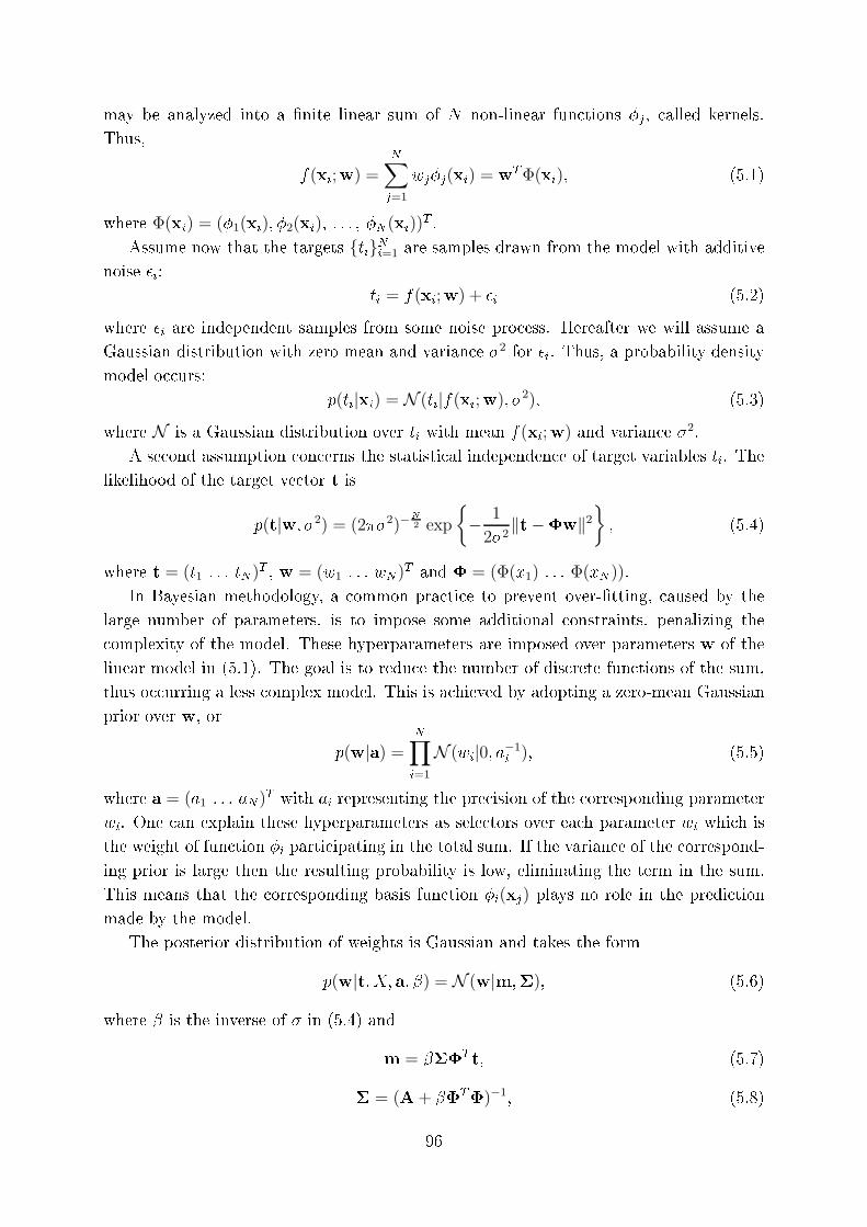
may be analyzed into a �nite linear sum of N non-linear fun tions �

j

, alled kernels.

Thus,

f(xi

;w) =

N∑

j=1

w

j

�

j

(xi

) = w

TΦ(xi

); (5.1)

where Φ(xi

) = (�1(xi); �2(xi); : : : ; �N(xi))T

.

Assume now that the targets {ti

}Ni=1 are samples drawn from the model with additive

noise �

i

:

t

i

= f(xi

;w) + �

i

(5.2)

where �

i

are independent samples from some noise pro ess. Hereafter we will assume a

Gaussian distribution with zero mean and varian e �

2for �

i

. Thus, a probability density

model o urs:

p(ti

|xi

) = N (ti

|f(xi

;w); �2); (5.3)

where N is a Gaussian distribution over t

i

with mean f(xi

;w) and varian e �

2.

A se ond assumption on erns the statisti al independen e of target variables t

i

. The

likelihood of the target ve tor t is

p(t|w; �2) = (2��2)−N

2 exp

{

− 1

2�2‖t−�w‖2

}

; (5.4)

where t = (t1 : : : tN)T

, w = (w1 : : : wN

)T and � = (Φ(x1) : : : Φ(xN )).

In Bayesian methodology, a ommon pra ti e to prevent over-�tting, aused by the

large number of parameters, is to impose some additional onstraints, penalizing the

omplexity of the model. These hyperparameters are imposed over parameters w of the

linear model in (5.1). The goal is to redu e the number of dis rete fun tions of the sum,

thus o urring a less omplex model. This is a hieved by adopting a zero-mean Gaussian

prior over w, or

p(w|a) =N∏

i=1

N (wi

|0; a−1i

); (5.5)

where a = (a1 : : : aN)T

with a

i

representing the pre ision of the orresponding parameter

w

i

. One an explain these hyperparameters as sele tors over ea h parameter w

i

whi h is

the weight of fun tion �

i

parti ipating in the total sum. If the varian e of the orrespond-

ing prior is large then the resulting probability is low, eliminating the term in the sum.

This means that the orresponding basis fun tion �

i

(xj

) plays no role in the predi tion

made by the model.

The posterior distribution of weights is Gaussian and takes the form

p(w|t; X; a; �) = N (w|m;�); (5.6)

where � is the inverse of � in (5.4) and

m = ��

T

t; (5.7)

� = (A+ ��

T

�)−1; (5.8)

96

with A = diag{ai

}.Eventually, an iterative learning pro ess o urs. Initially, we hoose some values for a,

�, thus evaluating the mean and ovarian e of the posterior using (5.7) and (5.8). Then

we iterate, until a onvergen e riterion is satis�ed, by re-estimating the hyperparameters:

a

i

=

i

m

2i

; (5.9)

�

−1 =‖t−�m‖2N −∑N

i=1 i

; (5.10)

where m

i

is the i

th

omponent of the posterior mean de�ned by (5.7). and the quantity

i

is omputed as:

i

= 1− a

i

Σii

; (5.11)

where Σii

is the i

th

diagonal omponent of the ovarian e matrix � given by (5.8).

The result of the training pro ess des ribed above is learning parameters w of equation

(5.1).

97

Author's Publi ations

Journal Publi ations

J1 D. Gerogiannis, C. Nikou and A. Likas. The mixtures of Student's t-distributions as

a robust framework for rigid registration. Image and Vision Computing, Vol.

27, No 9, pp. 1285-1294, 2009.

J2 D. Gerogiannis, C. Nikou and A. Likas. Registering sets of points using Bayesian

regression. Neuro omputing, Vol. 89, pp.122-133, 2012.

J3 D. Gerogiannis, C. Nikou and A. Likas. Modeling sets of unordered points using highly

e entri ellipses. EURASIP Journal on Advan es in Signal Pro essing,

2014:11, 2014.

J4 D. Gerogiannis, C. Nikou and A. Likas. Elimination of outliers from 2D point sets

using the Helmholtz prin iple. Submitted.

Conferen e Publi ations

C1 D. Gerogiannis, C. Nikou and A. Likas. Rigid image registration based on pixel

grouping. In Pro eedings of the 14th International Conferen e on Image Analysis

and Pro essing (ICIAP'07), 10-14 September 2007, Modena, Italy.

C2 D. Gerogiannis, C. Nikou and A. Likas. Robust image registration using mixtures of

t-distributions. Pro eedings of the 8th IEEE Computer So iety Workshop on Math-

emati al Methods in Biomedi al Image Analysis (MMBIA'07), in onjun tion with

ICCV'07, 14-20 O tober 2007, Rio de Janeiro, Brazil.

C3 D. Gerogiannis, C. Nikou and A. Likas. A split-and-merge framework for 2D shape

summarization. 7th International Symposium on Image and Signal Pro essing and

Analysis (ISPA'11), pp. 206-2011, 4-6 September 2011, Dubrovnik, Croatia.

The reader may �nd a digital opy of all the above publi ations at my personal a ademi webpage

(www. s.uoi.gr/∼dgerogia).

C4 D. Gerogiannis, C. Nikou and A. Likas. Fast and eÆ ient vanishing point dete tion

in indoor images. International Conferen e on Pattern Re ognition (ICPR'12), pp.

3244-3247, 11-15 November 2012, Tsukuba, Japan.

C5 D. Gerogianis, C. Nikou and A. Likas. Global sampling of image edges. IEEE In-

ternational Conferen e on Image Pro essing (ICIP'14), 27-30 O tober 2014, Paris,

Fran e.

C6 D. Gerogiannis, C. Nikou and L. P. Kondi. Shape en oding for edge map image

ompression. Submitted.

Other publi ations not related to this thesis

P1 D. Gerogiannis, C. Nikou. Tex-Lex: Automated generation of texture lexi ons us-

ing images from the World Wide Web. International Conferen e on Digital Signal

Pro essing (DSP'13), 1-3 July 2013, Santorini, Gree e.

P2 A. Giotis, D. Gerogiannis and C. Nikou. Word spotting in handwritten text using

ontour-based models. 14th International Conferen e on Frontiers in Handwriting

Re ognition (ICFHR'14), 1-4 September 2014, Hersonisos, Crete, Gree e, pp. 399-

404, 2014.

P3 D. Gerogiannis, S. A. So�anos, I. E. Lagaris, G. A. Evangelakis. One-Dimensional

Inverse S attering Problem in A ousti s, Brazilian Journal of Physi s, Vol. 41,

pp. 248-257, 2011.

Short Vita

I was born in Ioannina, Gree e in February 1983. I re eived my BS and MS both from

the Department of Computer S ien e, University of Ioannina in 2004 and 2007 respe tively

and sin e 2008 I am a Phd andidate at the same Department. I am an a tive resear her

in omputer vision and my resear h interests in lude image segmentation and registration,

point set registration, feature extra tion, pattern re ognition and autonomous navigation.

I am an IEEE Student Member and from O tober 2012 till June 2013 I was the interim

Chair of the IEEE student bran h of the University of Ioannina. Sin e my early years in

the University, I was interested in entrepreneurship. I have setup two startups till now,

one involved in video-on-demand advertisements and one with digital marketing solutions

for mobile devi es. During those years I have parti ipated in various international and

lo al business ontests. In the past, I have worked as an instru tor at the Department of

Informati s and Tele ommuni ation of the Te hnologi al Edu ational Institute of Epirus,

Gree e.

Documents

Feature extraction for image and point set analysis