Embed Size (px)
Citation preview

February 14, 2005 Topic 3 1
Telecommunications EngineeringTopic 3: Modulation and FDMAJames K Beard, Ph.D.(215) [email protected]://astro.temple.edu/~jkbeard/
Topic 3 2February 14, 2005
Attendance
0
5
10
15
20
25
19-J
an
26-J
an
2-F
eb
9-F
eb
16-F
eb
23-F
eb
2-M
ar
9-M
ar
16-M
ar
23-M
ar
30-M
ar
6-A
pr
13-A
pr
20-A
pr
27-A
pr
Topic 3 3February 14, 2005
Topics
The Survey Homework
Problem 3.30, p. 177, Adjacent channel interference Problem 3.35 p. 178, look at part (a); part (b) was
done in class Problem 3.36 p. 178, an intermediate difficulty
problem in bit error rate using MSK Topics
Why follow sampling with coding? Shannon’s information theory
Topic 3 4February 14, 2005
Survey Thumbnail
Nine completed surveys Six incomplete or just looks Five did not open the survey Selection biases results?
Only 45% of class gives all resultsOther 55% can be best, worst, or more of the
same
Topic 3 5February 14, 2005
Multiple Choice Questions
All are replies on 1-5 basis No answers were 1 or 5 Questions
My background is appropriate I understand sampled time/frequency domains I am comfortable with readings and text
Topic 3 6February 14, 2005
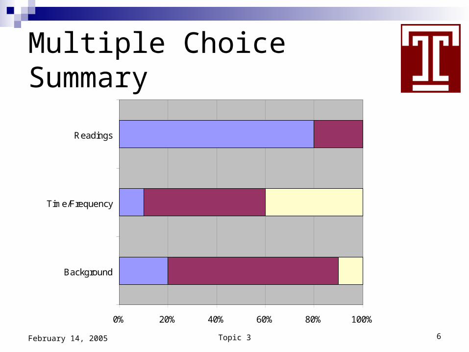
Multiple Choice Summary
0% 20% 40% 60% 80% 100%
Background
Time/Frequency
Readings
Topic 3 7February 14, 2005
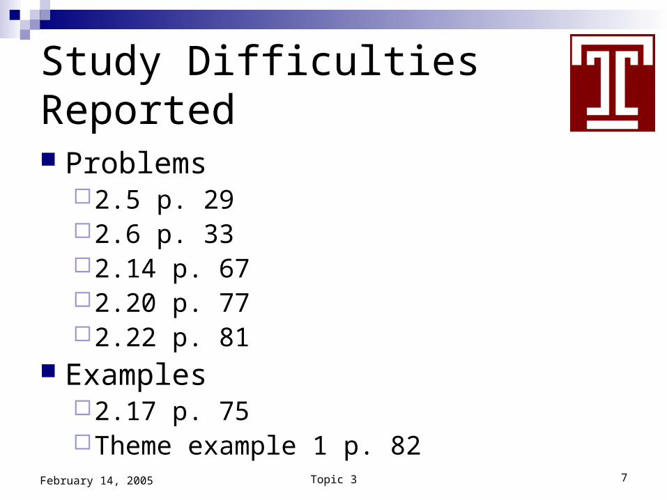
Study Difficulties Reported
Problems2.5 p. 292.6 p. 332.14 p. 672.20 p. 772.22 p. 81
Examples2.17 p. 75Theme example 1 p. 82
Topic 3 8February 14, 2005
Suggestions
More examples and homework problems worked through – already in progress
Go over more difficult homework problems before they are assigned
Warn and correct wrong answers – AIP Discuss WHY as well as HOW
Topic 3 9February 14, 2005
Survey Summary
Everybody is OKBased on 40% sampleBut, nobody answered 5’s
NeedMore coverage of how and whyFill in for prerequisites
Topic 3 10February 14, 2005
Homework
Problem 3.30, p. 177, Adjacent channel interference
Problem 3.35 p. 178, look at part (a); part (b) was done in class
Problem 3.36 p. 178, an intermediate difficulty problem in bit error rate using MSK
Topic 3 11February 14, 2005
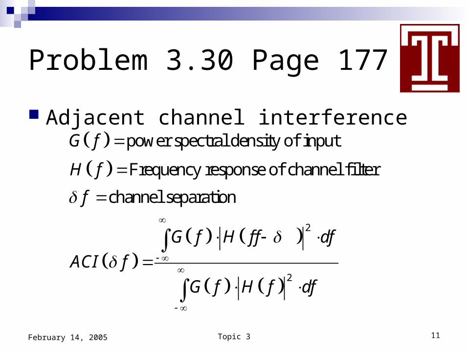
Problem 3.30 Page 177
Adjacent channel interference
2
2
power spectral density of input
Frequency response of channel filter
channel separation
G f
H f
f
G f H f f df
ACI f
G f H f df
Topic 3 12February 14, 2005
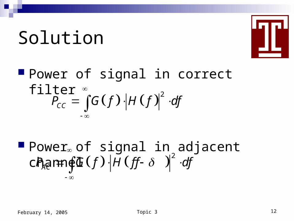
Solution
Power of signal in correct filter
Power of signal in adjacent channel
2
CCP G f H f df
2
ACP G f H f f df
Topic 3 13February 14, 2005
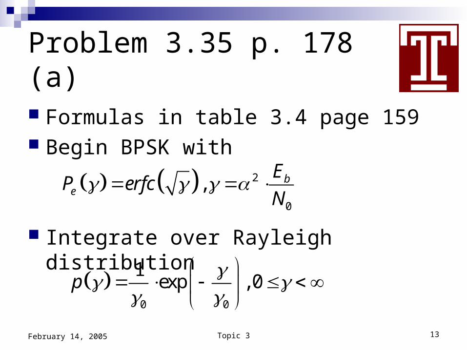
Problem 3.35 p. 178 (a)
Formulas in table 3.4 page 159 Begin BPSK with
Integrate over Rayleigh distribution
2
0
, be
EP erfc
N
0 0
1exp , 0p
Topic 3 14February 14, 2005
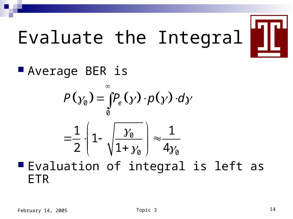
Evaluate the Integral
Average BER is
Evaluation of integral is left as ETR
0
0
0
0 0
1 11
2 1 4
eP P p d
Topic 3 15February 14, 2005
Problem 3.36 p. 178
Use MSK with a BER of 10-4 or better AWGN
Use Table 3.4 or Figure 3.32, pp. 159-160SNR requirement is about 8.3 dB
Rayleigh fadingUse Table 3.4 p. 159Solve for SNR of about 34 dB
Topic 3 16February 14, 2005
Coding Follows Sampling
SamplingSimply converts base signal to elementary
modulation formFormatting for performance is left to coding
CodingRemoval of redundancy == source codingChannel coding == error detection and
correction capability added
Topic 3 17February 14, 2005
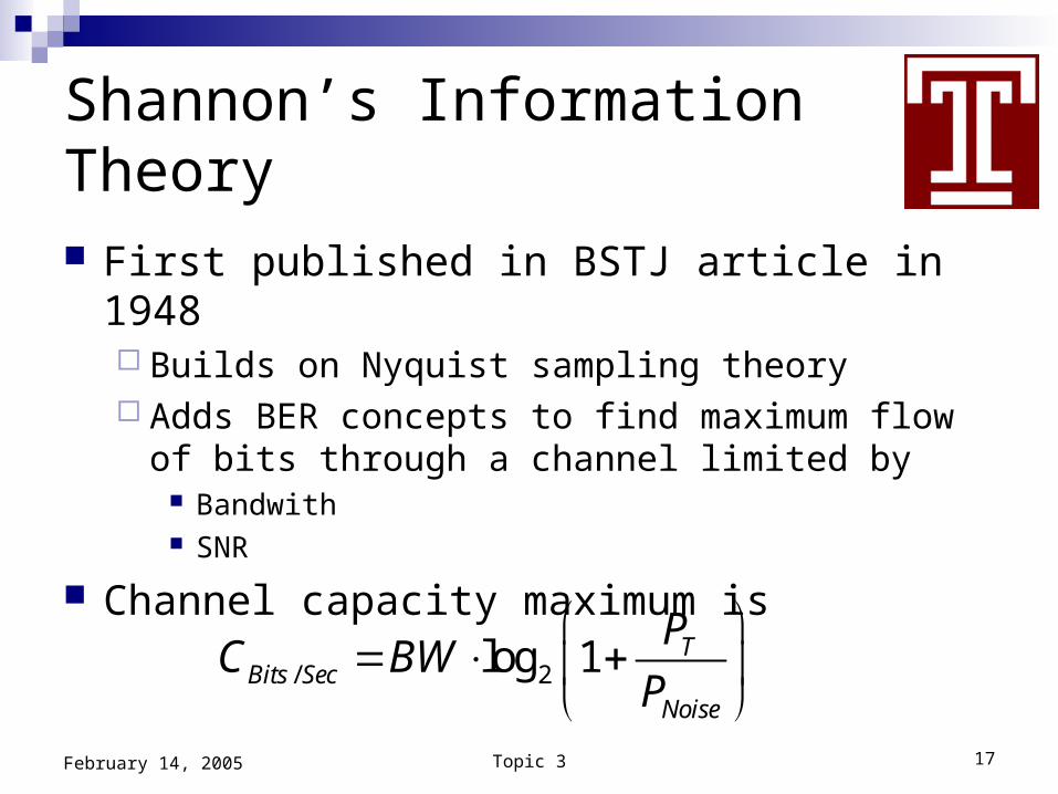
Shannon’s Information Theory
First published in BSTJ article in 1948 Builds on Nyquist sampling theory Adds BER concepts to find maximum flow of bits
through a channel limited by Bandwith SNR
Channel capacity maximum is
/ 2log 1 TBits Sec
Noise
PC BW
P
Topic 3 18February 14, 2005
Other Important Results
Channel-coding theorem Given
A channel capacity CB/S
Channel bit rate less than channel capacity
Then There exists a coding scheme that achieves an arbitrarily
high BER
Rate distortion theory – sampling and data compression losses exempt from channel-coding theorem
Topic 3 19February 14, 2005
Concept of Entropy
Definition – Average information content per symbol
ImportanceFundamental limit on average number of bits
per source symbolChannel-coding theorem is stated in terms of
entropy
Topic 3 20February 14, 2005
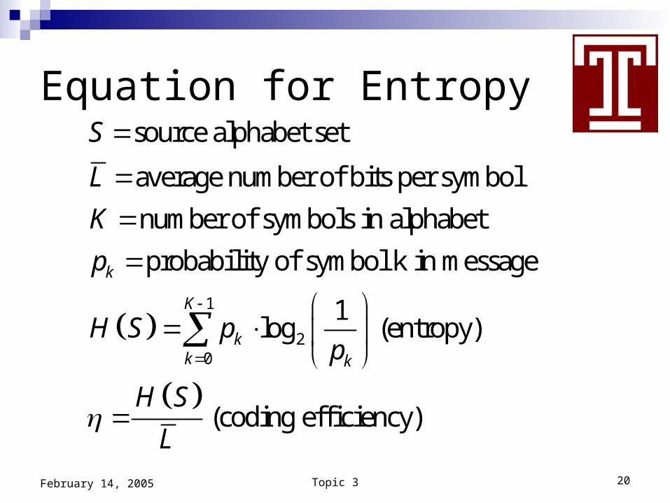
Equation for Entropy
1
20
source alphabet set
average number of bits per symbol
number of symbols in alphabet
probability of symbol k in message
1log (entropy)
(coding efficiency)
k
K
kk k
S
L
K
p
H S pp
H S
L
Topic 3 21February 14, 2005
Study Problems and Reading Assignments Reading assignments
Read Section 4.6, Cyclic Redundancy ChecksRead Section 4.7, Error-Control Coding
Study examplesExample 4.1 page 197Problem 4.1 page 197
Topic 3 22February 14, 2005
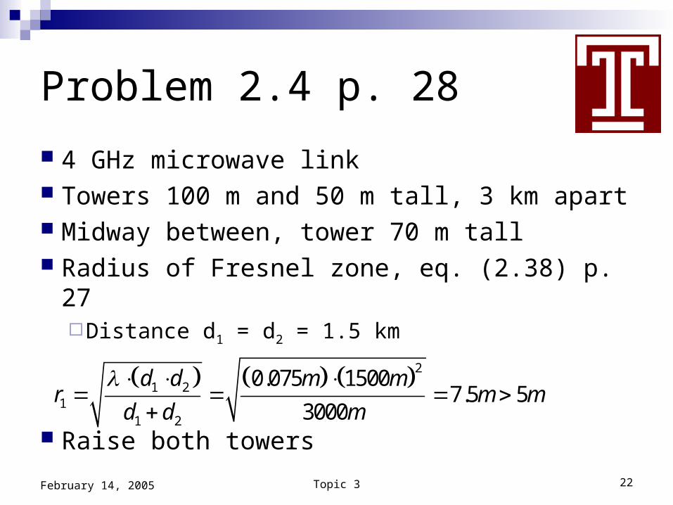
Problem 2.4 p. 28
4 GHz microwave link Towers 100 m and 50 m tall, 3 km apart Midway between, tower 70 m tall Radius of Fresnel zone, eq. (2.38) p. 27
Distance d1 = d2 = 1.5 km
Raise both towers
2
1 21
1 2
0.075 15007.5 5
3000
d d m mr m m
d d m
Topic 3 23February 14, 2005
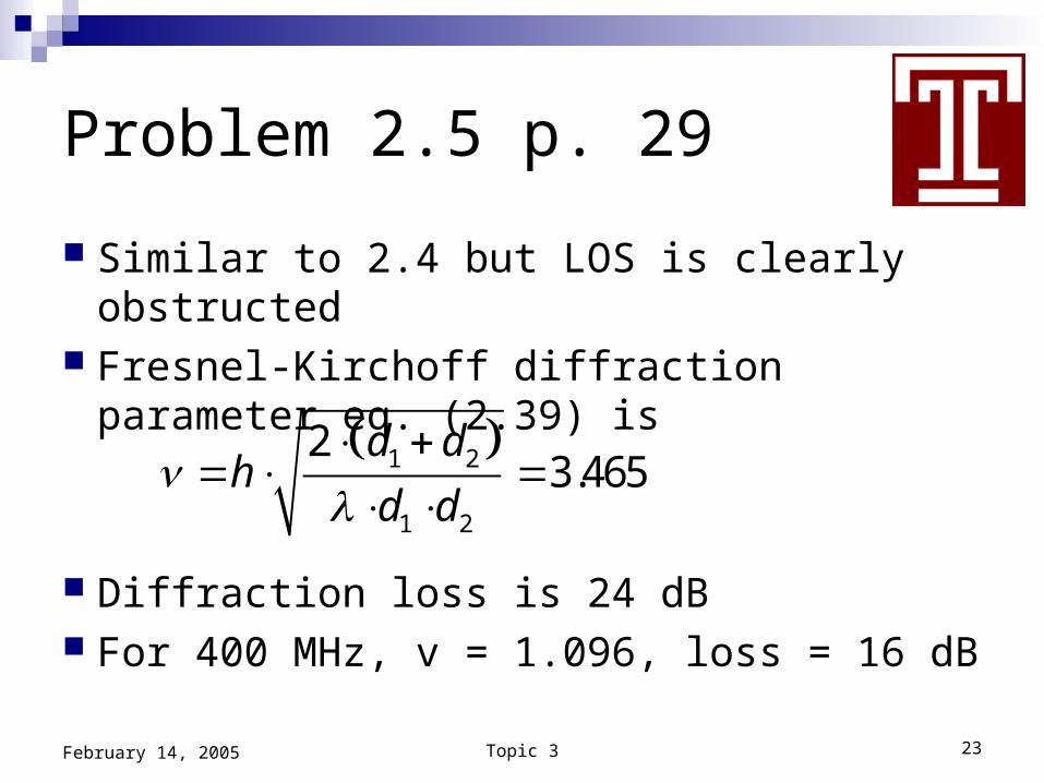
Problem 2.5 p. 29
Similar to 2.4 but LOS is clearly obstructed Fresnel-Kirchoff diffraction parameter eq.
(2.39) is
Diffraction loss is 24 dB For 400 MHz, v = 1.096, loss = 16 dB
1 2
1 2
23.465
d dh
d d
Topic 3 24February 14, 2005
Term Projects Areas for coverage
Propagation and noise Free space Urban
Modulation & FDMACodingDemodulation and detection
Will deploy over Blackboard this week
Topic 3 25February 14, 2005
Term Project Timeline
First week Parse and report your understanding Give estimated parameters including SystemView
system clock rate Second week
Block out SystemView Signal generator Modulator
Through mid-April Flesh out as class topics are presented Due date TBD

February 14, 2005 Topic 3 26
EE320 Digital Telecommunications
Quiz 1 Report
February 21, 2005
Topic 3 27February 14, 2005
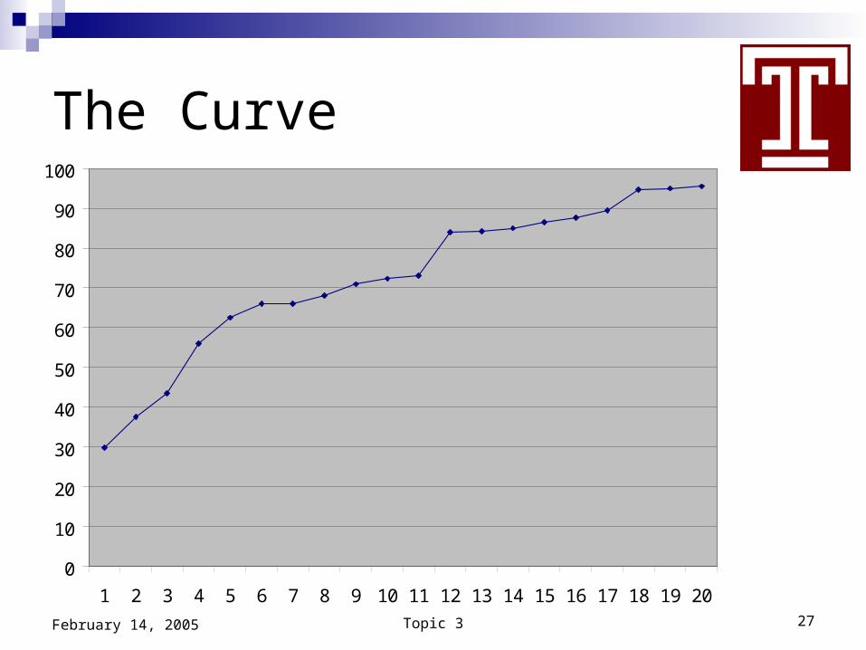
The Curve
0
10
20
30
40
50
60
70
80
90
100
1 2 3 4 5 6 7 8 9 10 11 12 13 14 15 16 17 18 19 20
Topic 3 28February 14, 2005
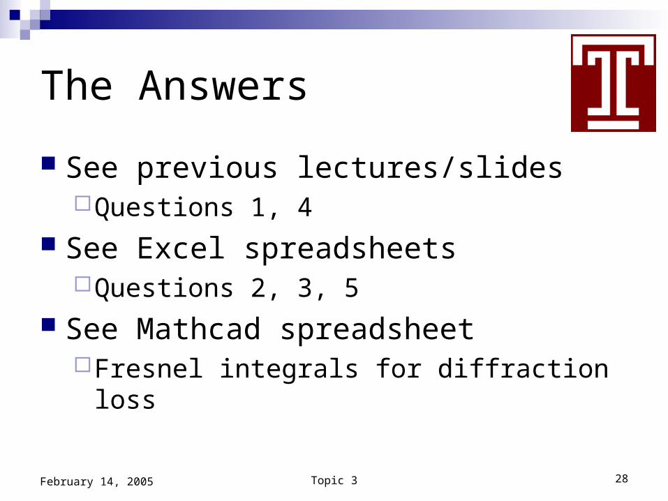
The Answers
See previous lectures/slidesQuestions 1, 4
See Excel spreadsheetsQuestions 2, 3, 5
See Mathcad spreadsheetFresnel integrals for diffraction loss
Topic 3 29February 14, 2005
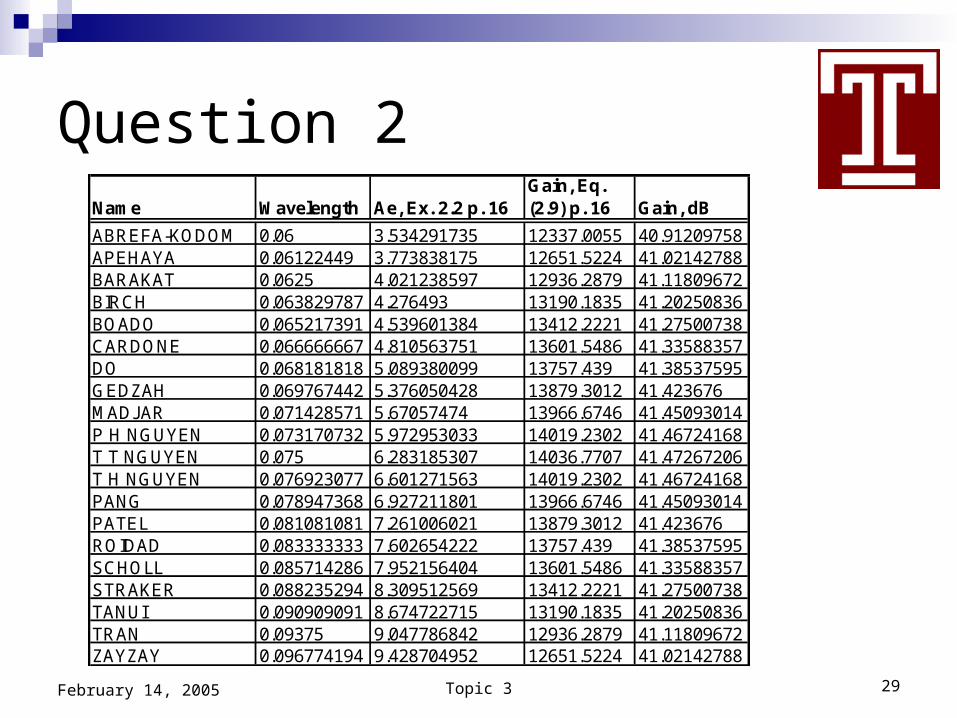
Question 2Name Wavelength Ae, Ex. 2.2 p. 16
Gain, Eq. (2.9) p. 16 Gain, dB
ABREFA-KODOM 0.06 3.534291735 12337.0055 40.91209758APEHAYA 0.06122449 3.773838175 12651.5224 41.02142788BARAKAT 0.0625 4.021238597 12936.2879 41.11809672BIRCH 0.063829787 4.276493 13190.1835 41.20250836BOADO 0.065217391 4.539601384 13412.2221 41.27500738CARDONE 0.066666667 4.810563751 13601.5486 41.33588357DO 0.068181818 5.089380099 13757.439 41.38537595GEDZAH 0.069767442 5.376050428 13879.3012 41.423676MADJAR 0.071428571 5.67057474 13966.6746 41.45093014P H NGUYEN 0.073170732 5.972953033 14019.2302 41.46724168T T NGUYEN 0.075 6.283185307 14036.7707 41.47267206T H NGUYEN 0.076923077 6.601271563 14019.2302 41.46724168PANG 0.078947368 6.927211801 13966.6746 41.45093014PATEL 0.081081081 7.261006021 13879.3012 41.423676ROIDAD 0.083333333 7.602654222 13757.439 41.38537595SCHOLL 0.085714286 7.952156404 13601.5486 41.33588357STRAKER 0.088235294 8.309512569 13412.2221 41.27500738TANUI 0.090909091 8.674722715 13190.1835 41.20250836TRAN 0.09375 9.047786842 12936.2879 41.11809672ZAYZAY 0.096774194 9.428704952 12651.5224 41.02142788
Topic 3 30February 14, 2005
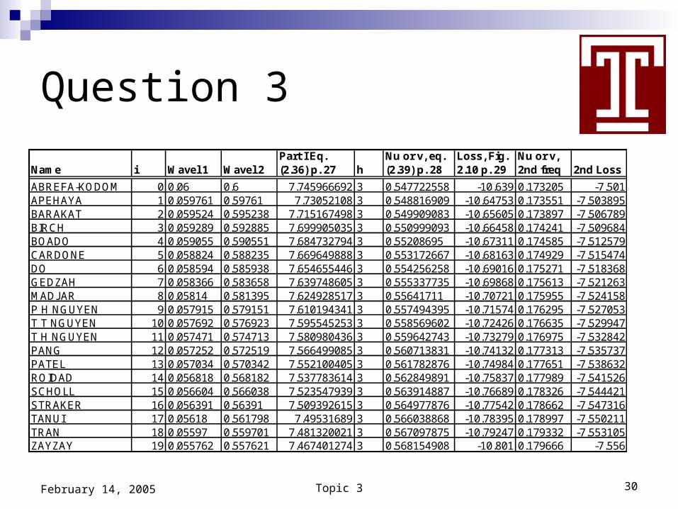
Question 3
Name i Wavel 1 Wavel 2Part I Eq. (2.36) p. 27 h
Nu or v, eq. (2.39) p. 28
Loss, Fig. 2.10 p. 29
Nu or v, 2nd freq 2nd Loss
ABREFA-KODOM 0 0.06 0.6 7.745966692 3 0.547722558 -10.639 0.173205 -7.501APEHAYA 1 0.059761 0.59761 7.73052108 3 0.548816909 -10.64753 0.173551 -7.503895BARAKAT 2 0.059524 0.595238 7.715167498 3 0.549909083 -10.65605 0.173897 -7.506789BIRCH 3 0.059289 0.592885 7.699905035 3 0.550999093 -10.66458 0.174241 -7.509684BOADO 4 0.059055 0.590551 7.684732794 3 0.55208695 -10.67311 0.174585 -7.512579CARDONE 5 0.058824 0.588235 7.669649888 3 0.553172667 -10.68163 0.174929 -7.515474DO 6 0.058594 0.585938 7.654655446 3 0.554256258 -10.69016 0.175271 -7.518368GEDZAH 7 0.058366 0.583658 7.639748605 3 0.555337735 -10.69868 0.175613 -7.521263MADJAR 8 0.05814 0.581395 7.624928517 3 0.55641711 -10.70721 0.175955 -7.524158P H NGUYEN 9 0.057915 0.579151 7.610194341 3 0.557494395 -10.71574 0.176295 -7.527053T T NGUYEN 10 0.057692 0.576923 7.595545253 3 0.558569602 -10.72426 0.176635 -7.529947T H NGUYEN 11 0.057471 0.574713 7.580980436 3 0.559642743 -10.73279 0.176975 -7.532842PANG 12 0.057252 0.572519 7.566499085 3 0.560713831 -10.74132 0.177313 -7.535737PATEL 13 0.057034 0.570342 7.552100405 3 0.561782876 -10.74984 0.177651 -7.538632ROIDAD 14 0.056818 0.568182 7.537783614 3 0.562849891 -10.75837 0.177989 -7.541526SCHOLL 15 0.056604 0.566038 7.523547939 3 0.563914887 -10.76689 0.178326 -7.544421STRAKER 16 0.056391 0.56391 7.509392615 3 0.564977876 -10.77542 0.178662 -7.547316TANUI 17 0.05618 0.561798 7.49531689 3 0.566038868 -10.78395 0.178997 -7.550211TRAN 18 0.05597 0.559701 7.481320021 3 0.567097875 -10.79247 0.179332 -7.553105ZAYZAY 19 0.055762 0.557621 7.467401274 3 0.568154908 -10.801 0.179666 -7.556
Topic 3 31February 14, 2005
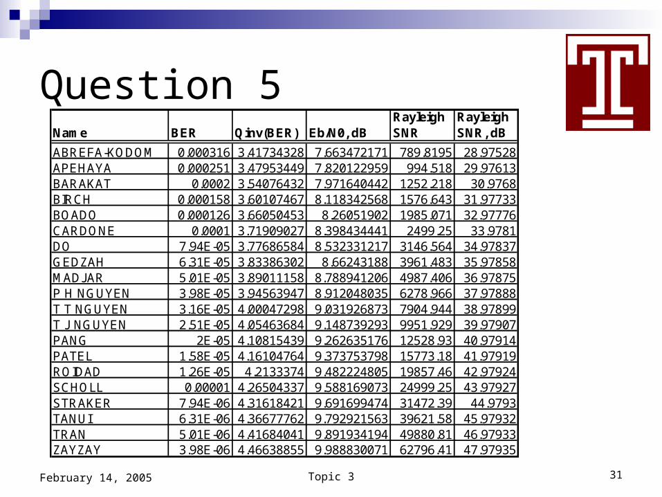
Question 5Name BER Qinv(BER) Eb/N0, dB
Rayleigh SNR
Rayleigh SNR, dB
ABREFA-KODOM 0.000316 3.41734328 7.663472171 789.8195 28.97528APEHAYA 0.000251 3.47953449 7.820122959 994.518 29.97613BARAKAT 0.0002 3.54076432 7.971640442 1252.218 30.9768BIRCH 0.000158 3.60107467 8.118342568 1576.643 31.97733BOADO 0.000126 3.66050453 8.26051902 1985.071 32.97776CARDONE 0.0001 3.71909027 8.398434441 2499.25 33.9781DO 7.94E-05 3.77686584 8.532331217 3146.564 34.97837GEDZAH 6.31E-05 3.83386302 8.66243188 3961.483 35.97858MADJAR 5.01E-05 3.89011158 8.788941206 4987.406 36.97875P H NGUYEN 3.98E-05 3.94563947 8.912048035 6278.966 37.97888T T NGUYEN 3.16E-05 4.00047298 9.031926873 7904.944 38.97899T J NGUYEN 2.51E-05 4.05463684 9.148739293 9951.929 39.97907PANG 2E-05 4.10815439 9.262635176 12528.93 40.97914PATEL 1.58E-05 4.16104764 9.373753798 15773.18 41.97919ROIDAD 1.26E-05 4.2133374 9.482224805 19857.46 42.97924SCHOLL 0.00001 4.26504337 9.588169073 24999.25 43.97927STRAKER 7.94E-06 4.31618421 9.691699474 31472.39 44.9793TANUI 6.31E-06 4.36677762 9.792921563 39621.58 45.97932TRAN 5.01E-06 4.41684041 9.891934194 49880.81 46.97933ZAYZAY 3.98E-06 4.46638855 9.988830071 62796.41 47.97935
Topic 3 32February 14, 2005
The Quiz in the Text (1 of 2)
Question 1 Text pp 3-5 Lectures and slides several times
Question 2 Antenna gain equations (2.2), (2.3) pp 14 Also equations (2.9), example 2.2, pp 16-17
Question 3 Section 2.3.2 and exa,[;e 2.3 pp 24-29 Two lectures, example worked in class, practice quiz
Topic 3 33February 14, 2005
The Quiz in the Text (2 of 2)
Question 4Problem 3.30 p. 177Given in classAnswer was to give equation that was given in
the problem statement Question 5
Problem 3.36, given in classUse table 3.4, figure 3.33, pp. 159-161
February 14, 2005 Topic 3 34
EE320 Convolutional Codes
James K Beard, Ph.D.
Topic 3 35February 14, 2005
Bonus Topic: Gray Codes
Sometimes called reflected codes Defining property: only one bit changes
between sequential codes Conversion
Binary codes to Gray Work from LSB up XOR of bits j and j+1 to get bit j of Gray code Bit past MSB of binary code is 0
Gray to binary Work from MSB down XOR bits j+1 of binary code and bit j of Gray code to get bit j
of binary code Bit past MSB of binary code is 0
Topic 3 36February 14, 2005
Polynomials Modulo 2
Definition Coefficients are ones and zeros Values of independent variable are one or zero Result of computation is taken modulo 2 – a one or
zero
The theory Well developed to support many DSP applications Mathematical theory includes finite fields and other
areas
Topic 3 37February 14, 2005
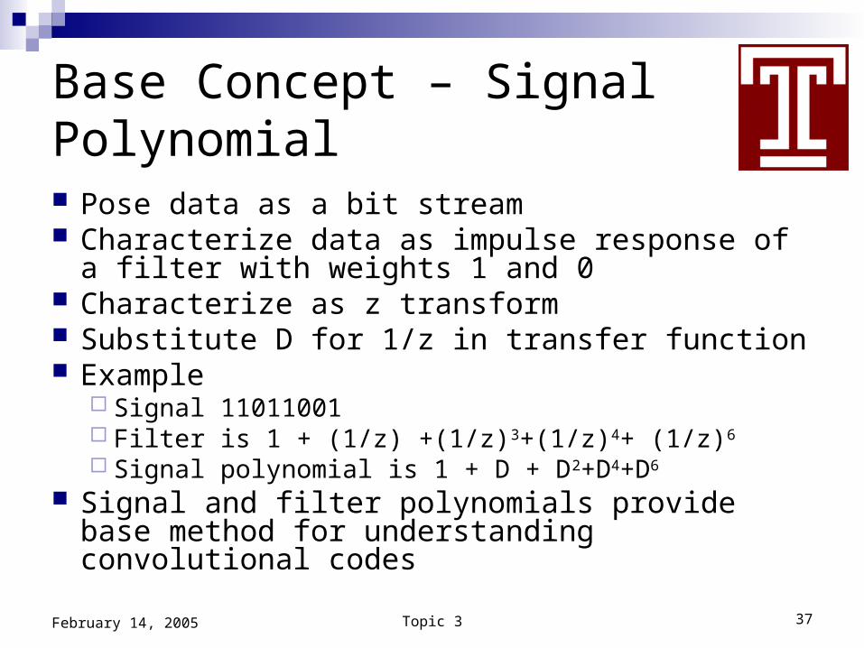
Base Concept – Signal Polynomial Pose data as a bit stream Characterize data as impulse response of a filter
with weights 1 and 0 Characterize as z transform Substitute D for 1/z in transfer function Example
Signal 11011001 Filter is 1 + (1/z) +(1/z)3+(1/z)4+ (1/z)6
Signal polynomial is 1 + D + D2+D4+D6
Signal and filter polynomials provide base method for understanding convolutional codes
Topic 3 38February 14, 2005
Base Concept –Modulo 2 Convolutions Scenario
Bitstream into convolution filterFilter weights are ones and zerosOutput is taken modulo 2 – i.e. a 1 or 0
Result: A modulo 2 convolution converts one bit stream into another
Topic 3 39February 14, 2005
Benefits of Concept
Convolution is product of polynomials Conventional multiplication of polynomials is
isomorphic to convolution of the sequence of their coefficients
Taking the resulting coefficients modulo 2 presents us with the output of a bitstream into a convolution filter with output modulo 2
These special polynomials have a highly developed mathematical basis
Implementation in hardware and software is very simple
Topic 3 40February 14, 2005
Error-Control Coding
Two categories of channel codingForward error-correction (EDAC)Automatic-repeat request (handshake)
CRC CodesHash codes of the messageError detection, but not correction
Topic 3 41February 14, 2005
Topics in Convolutional Codes
The node diagram is a block diagram Polynomial representations
Represent signals, convolutions and special polynomials and polynomial operations
Give us a simple way to understand and analyze convolutions Trellis diagrams
Give us a mechanism to represent convolution operations as a finite state machine
Provide a first step in visulaization of the finite state machine Node diagrams
Provide a simple visualization of the finite state machine Provide a basis for very simple implementation
Topic 3 42February 14, 2005
Convolutional Code Steps
Reduce the message to a bit stream Operate using modulo-2 convolutions
Convolution filter with short binary maskTake result modulo 2
Implemented with one-bit shift registers with multiplexer (see Figure 4.6 p. 196)
Topic 3 43February 14, 2005
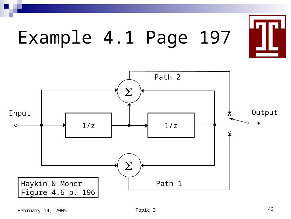
Example 4.1 Page 197
Output
1/z 1/z
Path 1
Path 2
Input
Haykin & MoherFigure 4.6 p. 196
Topic 3 44February 14, 2005
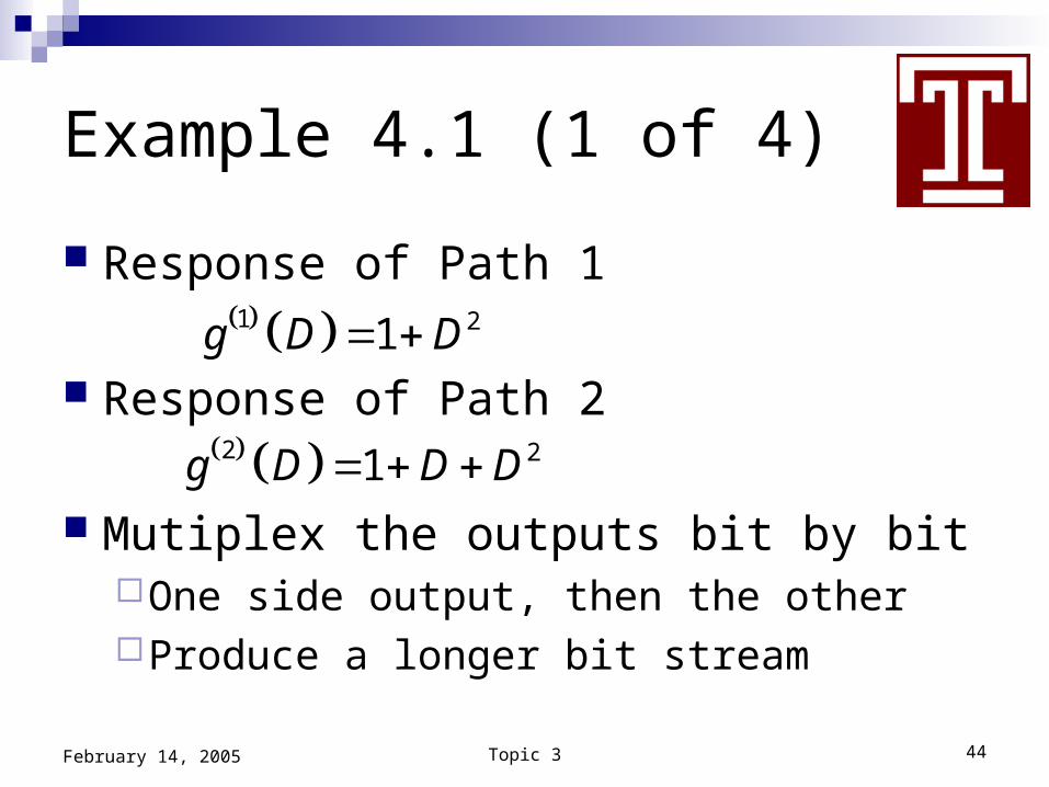
Example 4.1 (1 of 4)
Response of Path 1
Response of Path 2
Mutiplex the outputs bit by bitOne side output, then the otherProduce a longer bit stream
1 21g D D
2 21g D D D
Topic 3 45February 14, 2005
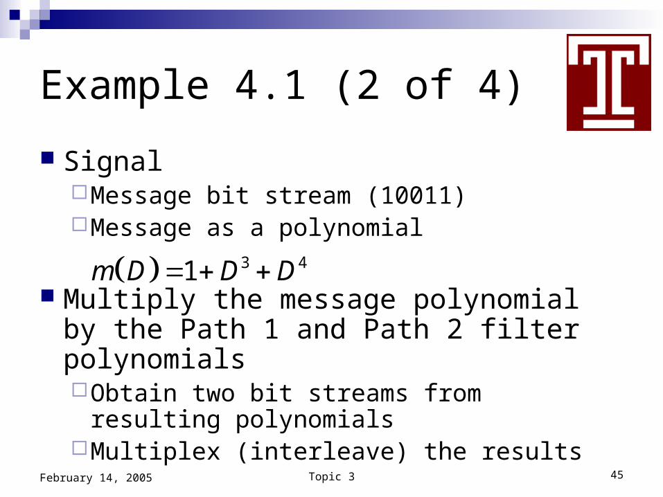
Example 4.1 (2 of 4)
SignalMessage bit stream (10011)Message as a polynomial
Multiply the message polynomial by the Path 1 and Path 2 filter polynomialsObtain two bit streams from resulting
polynomialsMultiplex (interleave) the results
3 41m D D D
Topic 3 46February 14, 2005
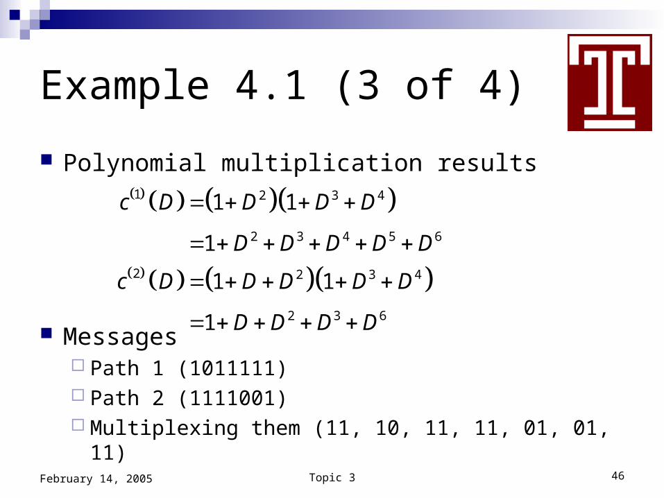
Example 4.1 (3 of 4)
Polynomial multiplication results
Messages Path 1 (1011111) Path 2 (1111001) Multiplexing them (11, 10, 11, 11, 01, 01, 11)
1 2 3 4
2 3 4 5 6
2 2 3 4
2 3 6
1 1
1
1 1
1
c D D D D
D D D D D
c D D D D D
D D D D
Topic 3 47February 14, 2005
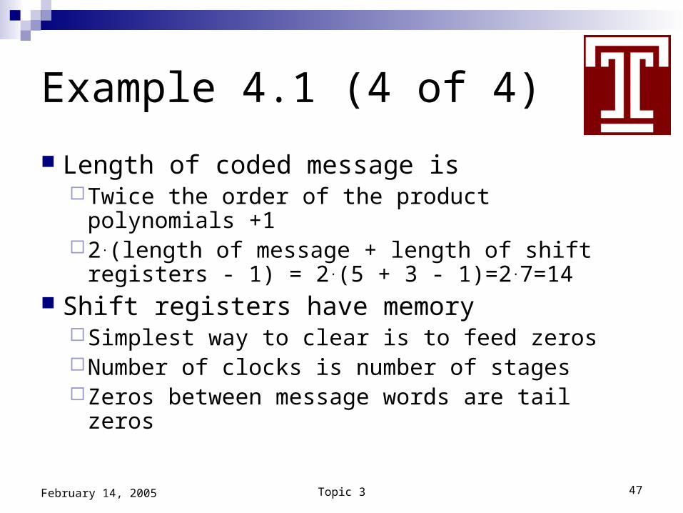
Example 4.1 (4 of 4)
Length of coded message isTwice the order of the product polynomials +12.(length of message + length of shift registers
- 1) = 2.(5 + 3 - 1)=2.7=14 Shift registers have memory
Simplest way to clear is to feed zerosNumber of clocks is number of stagesZeros between message words are tail zeros
Topic 3 48February 14, 2005
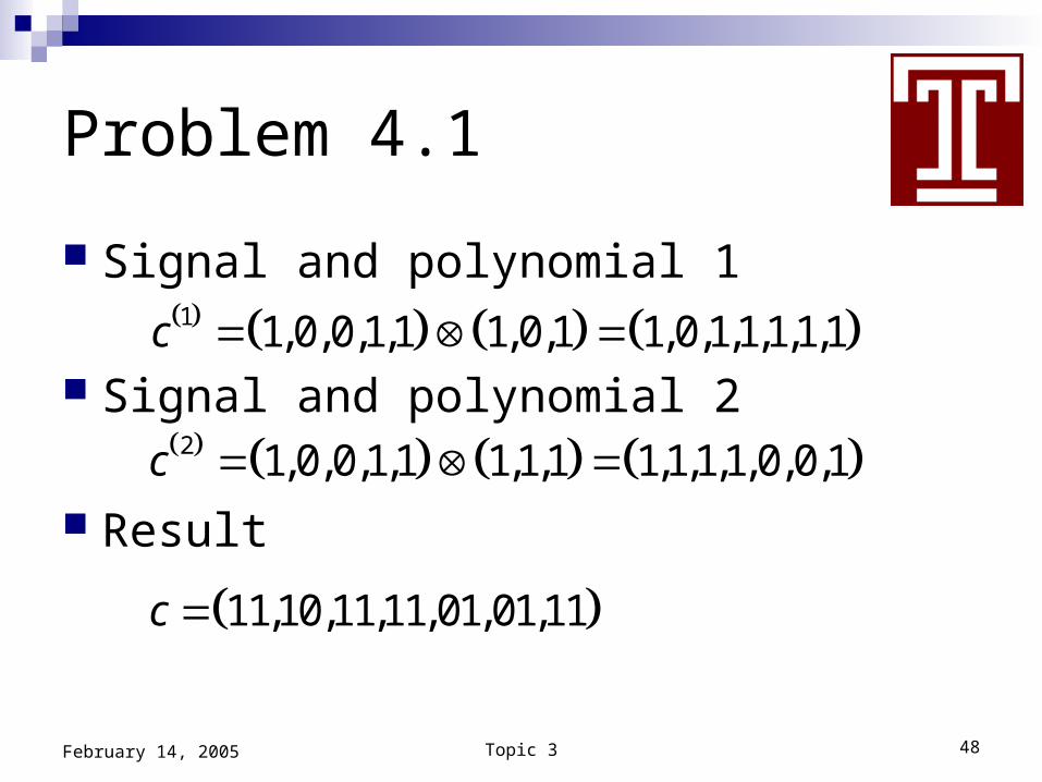
Problem 4.1
Signal and polynomial 1
Signal and polynomial 2
Result
1 1,0,0,1,1 1,0,1 1,0,1,1,1,1,1c
2 1,0,0,1,1 1,1,1 1,1,1,1,0,0,1c
11,10,11,11,01,01,11c
Topic 3 49February 14, 2005
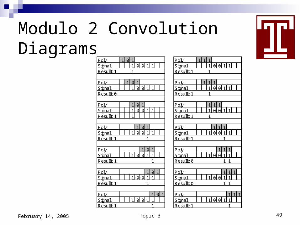
Modulo 2 Convolution Diagrams
Poly 1 0 1 Poly 1 1 1Signal 1 0 0 1 1 Signal 1 0 0 1 1Resullt: 1 1 Resullt: 1 1
Poly 1 0 1 Poly 1 1 1Signal 1 0 0 1 1 Signal 1 0 0 1 1Resullt: 0 Resullt: 1 1
Poly 1 0 1 Poly 1 1 1Signal 1 0 0 1 1 Signal 1 0 0 1 1Resullt: 1 1 Resullt: 1 1
Poly 1 0 1 Poly 1 1 1Signal 1 0 0 1 1 Signal 1 0 0 1 1Resullt: 1 1 Resullt: 1 1
Poly 1 0 1 Poly 1 1 1Signal 1 0 0 1 1 Signal 1 0 0 1 1Resullt: 1 1 Resullt: 0 1 1
Poly 1 0 1 Poly 1 1 1Signal 1 0 0 1 1 Signal 1 0 0 1 1Resullt: 1 1 Resullt: 0 1 1
Poly 1 0 1 Poly 1 1 1Signal 1 0 0 1 1 Signal 1 0 0 1 1Resullt: 1 1 Resullt: 1 1
Topic 3 50February 14, 2005
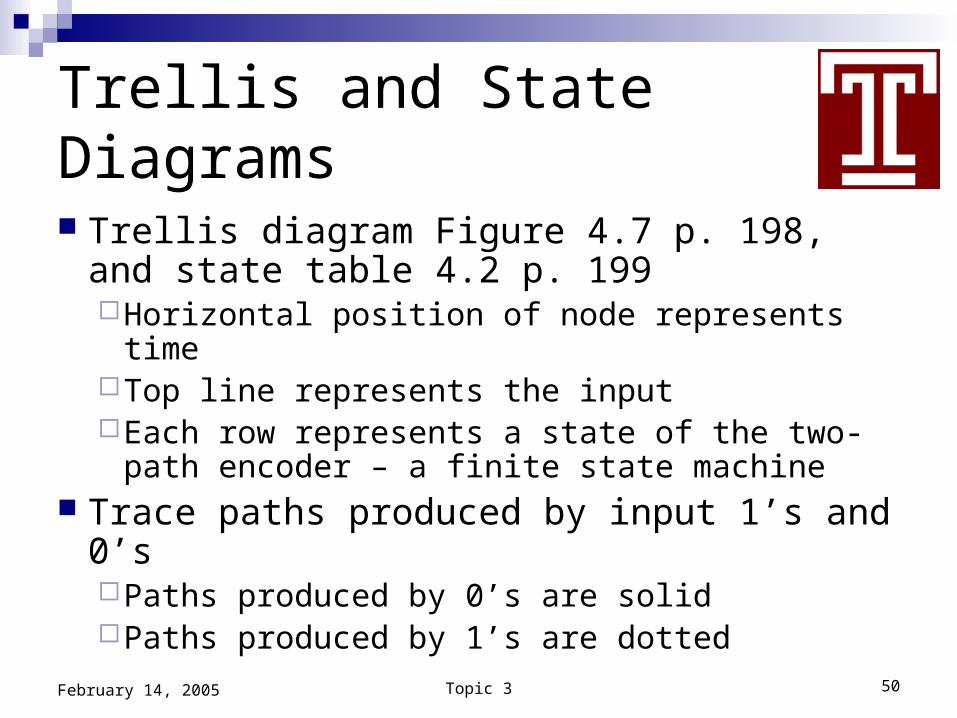
Trellis and State Diagrams
Trellis diagram Figure 4.7 p. 198, and state table 4.2 p. 199Horizontal position of node represents timeTop line represents the inputEach row represents a state of the two-path
encoder – a finite state machine Trace paths produced by input 1’s and 0’s
Paths produced by 0’s are solidPaths produced by 1’s are dotted
Topic 3 51February 14, 2005
Advantages of Trellis and State Diagrams Once drawn, output for any message is simple
to obtain Allowed and non-allowed state transitions are
explicit State diagram follows directly
Figure 4.8 p. 200 Shows state transitions and causes
Coding output of state diagram simpler than that of trellis diagram
Topic 3 52February 14, 2005
States of the Filter
We need the output states Ordered pair of bits from Path 1 and Path 2 Objective is tracing through states to get outputs
Output states not the same as register states Only four states can be defined from two outputs Total number of states is defined by the order of
convolution Current example is three taps Number of states is 2<order> or 8 We get to eight states by considering each pair of
consecutive input bits
Topic 3 53February 14, 2005
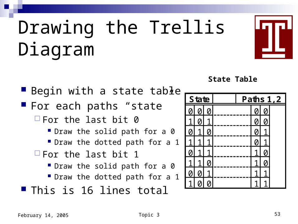
Drawing the Trellis Diagram
Begin with a state table For each paths “state”
For the last bit 0 Draw the solid path for a 0 Draw the dotted path for a 1
For the last bit 1 Draw the solid path for a 0 Draw the dotted path for a 1
This is 16 lines total
State Table
0 0 0 0 01 0 1 0 00 1 0 0 11 1 1 0 10 1 1 1 01 1 0 1 00 0 1 1 11 0 0 1 1
State Paths 1, 2
Topic 3 54February 14, 2005
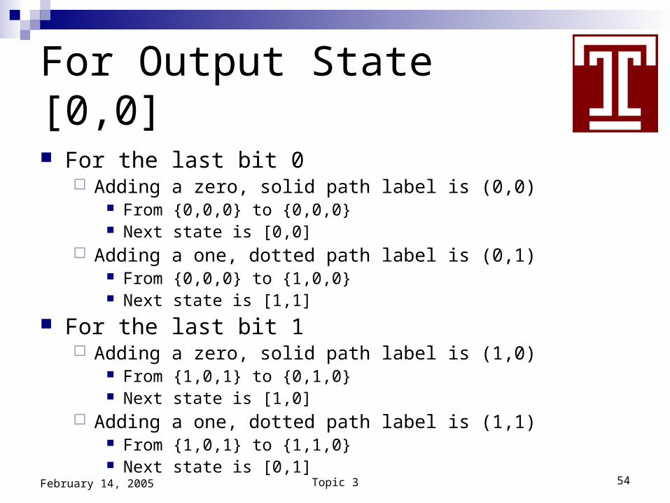
For Output State [0,0]
For the last bit 0 Adding a zero, solid path label is (0,0)
From {0,0,0} to {0,0,0} Next state is [0,0]
Adding a one, dotted path label is (0,1) From {0,0,0} to {1,0,0} Next state is [1,1]
For the last bit 1 Adding a zero, solid path label is (1,0)
From {1,0,1} to {0,1,0} Next state is [1,0]
Adding a one, dotted path label is (1,1) From {1,0,1} to {1,1,0} Next state is [0,1]
Topic 3 55February 14, 2005
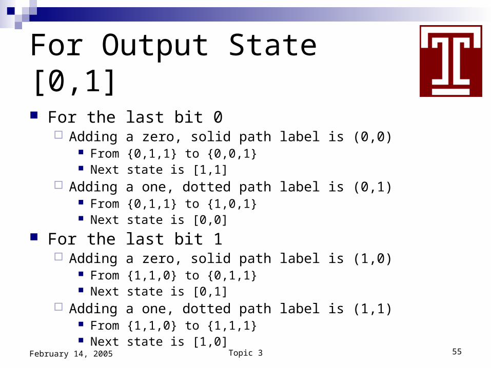
For Output State [0,1]
For the last bit 0 Adding a zero, solid path label is (0,0)
From {0,1,1} to {0,0,1} Next state is [1,1]
Adding a one, dotted path label is (0,1) From {0,1,1} to {1,0,1} Next state is [0,0]
For the last bit 1 Adding a zero, solid path label is (1,0)
From {1,1,0} to {0,1,1} Next state is [0,1]
Adding a one, dotted path label is (1,1) From {1,1,0} to {1,1,1} Next state is [1,0]
Topic 3 56February 14, 2005
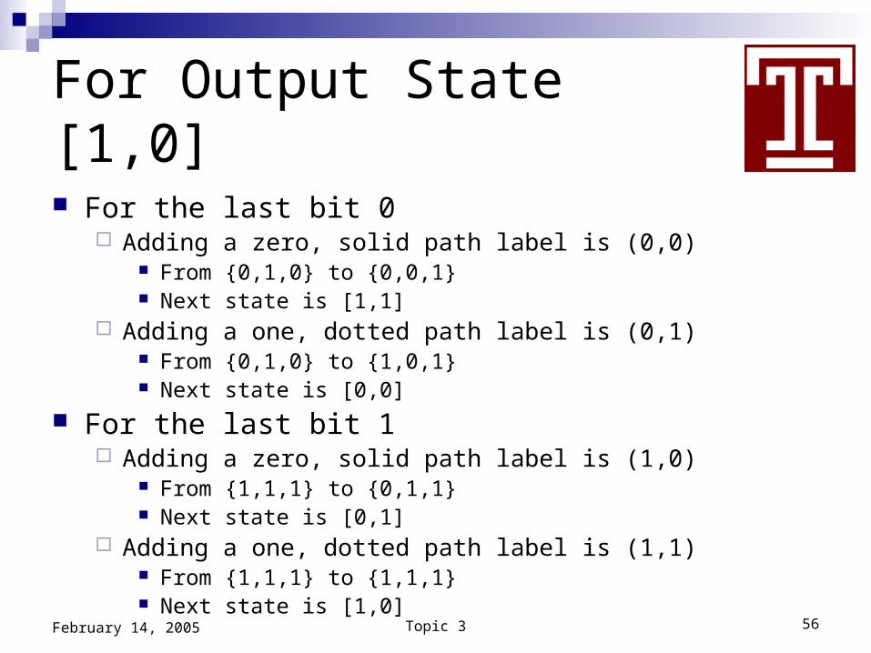
For Output State [1,0]
For the last bit 0 Adding a zero, solid path label is (0,0)
From {0,1,0} to {0,0,1} Next state is [1,1]
Adding a one, dotted path label is (0,1) From {0,1,0} to {1,0,1} Next state is [0,0]
For the last bit 1 Adding a zero, solid path label is (1,0)
From {1,1,1} to {0,1,1} Next state is [0,1]
Adding a one, dotted path label is (1,1) From {1,1,1} to {1,1,1} Next state is [1,0]
Topic 3 57February 14, 2005
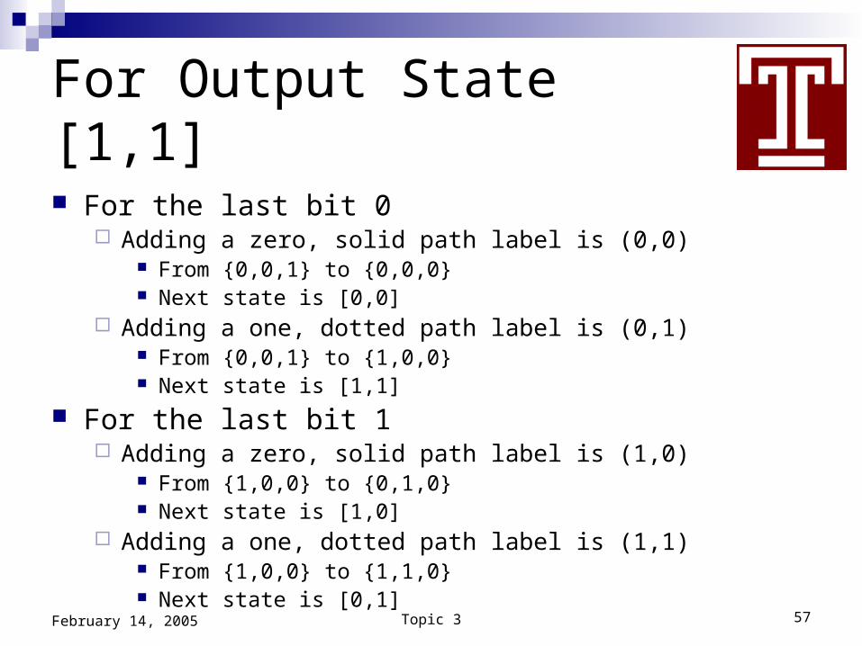
For Output State [1,1]
For the last bit 0 Adding a zero, solid path label is (0,0)
From {0,0,1} to {0,0,0} Next state is [0,0]
Adding a one, dotted path label is (0,1) From {0,0,1} to {1,0,0} Next state is [1,1]
For the last bit 1 Adding a zero, solid path label is (1,0)
From {1,0,0} to {0,1,0} Next state is [1,0]
Adding a one, dotted path label is (1,1) From {1,0,0} to {1,1,0} Next state is [0,1]
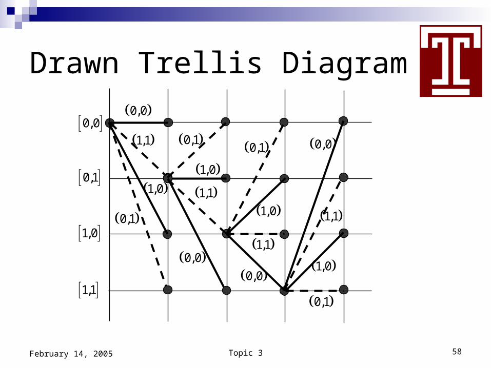
Topic 3 58February 14, 2005
Drawn Trellis Diagram
0,0
1,0
0,1
1,1
0,0
0,1
1,1
1,0
0,0
0,1
1,0
1,1
0,0
0,1
1,0
1,1
0,0
0,1
1,0
1,1
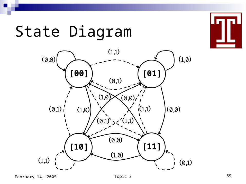
Topic 3 59February 14, 2005
State Diagram
[01][00]
[11][10]
0,0 1,0
0,1 1,1
1,1
1,1
1,1 0,0
0,0
0,0
1,0
1,0
1,0
0,1
0,1
0,1
February 14, 2005 Topic 3 60
EE320 Decoding Convolutional Codes
James K Beard, Ph.D.
Topic 3 61February 14, 2005
Where We are Going
Exploit the Channel Coding TheoremFor any required channel bit rate CR less than
the channel capacity C
A coding exists that achieves an arbitrarily low BER
Method is error-correcting codes
2log 1RC C B SNR
Topic 3 62February 14, 2005
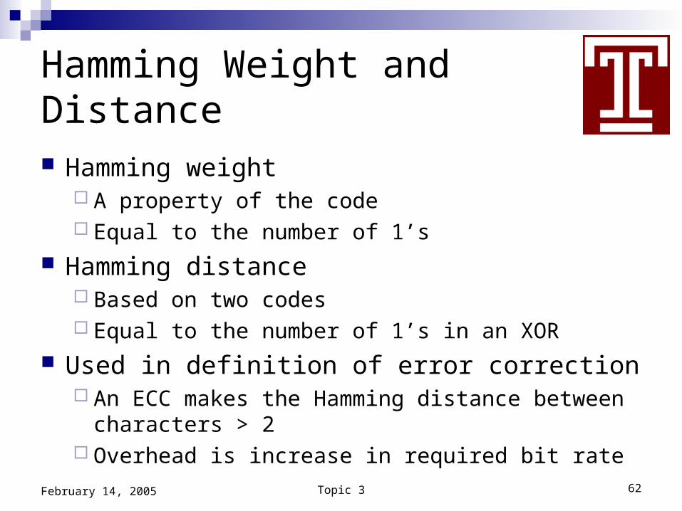
Hamming Weight and Distance
Hamming weight A property of the code Equal to the number of 1’s
Hamming distance Based on two codes Equal to the number of 1’s in an XOR
Used in definition of error correction An ECC makes the Hamming distance between
characters > 2 Overhead is increase in required bit rate
Topic 3 63February 14, 2005
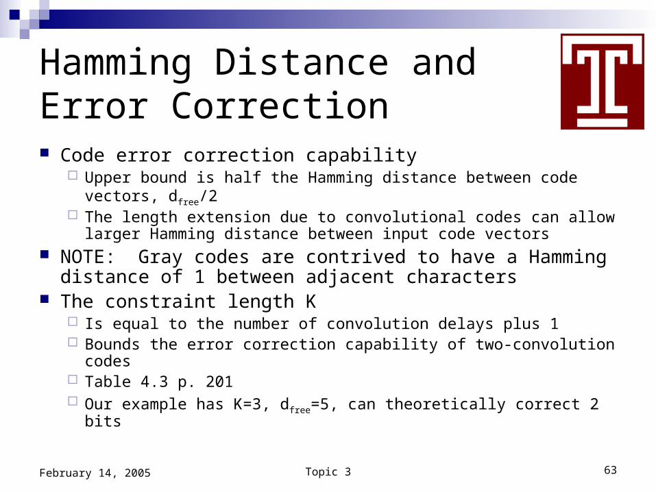
Hamming Distance and Error Correction Code error correction capability
Upper bound is half the Hamming distance between code vectors, dfree/2
The length extension due to convolutional codes can allow larger Hamming distance between input code vectors
NOTE: Gray codes are contrived to have a Hamming distance of 1 between adjacent characters
The constraint length K Is equal to the number of convolution delays plus 1 Bounds the error correction capability of two-convolution codes Table 4.3 p. 201 Our example has K=3, dfree=5, can theoretically correct 2 bits
Topic 3 64February 14, 2005
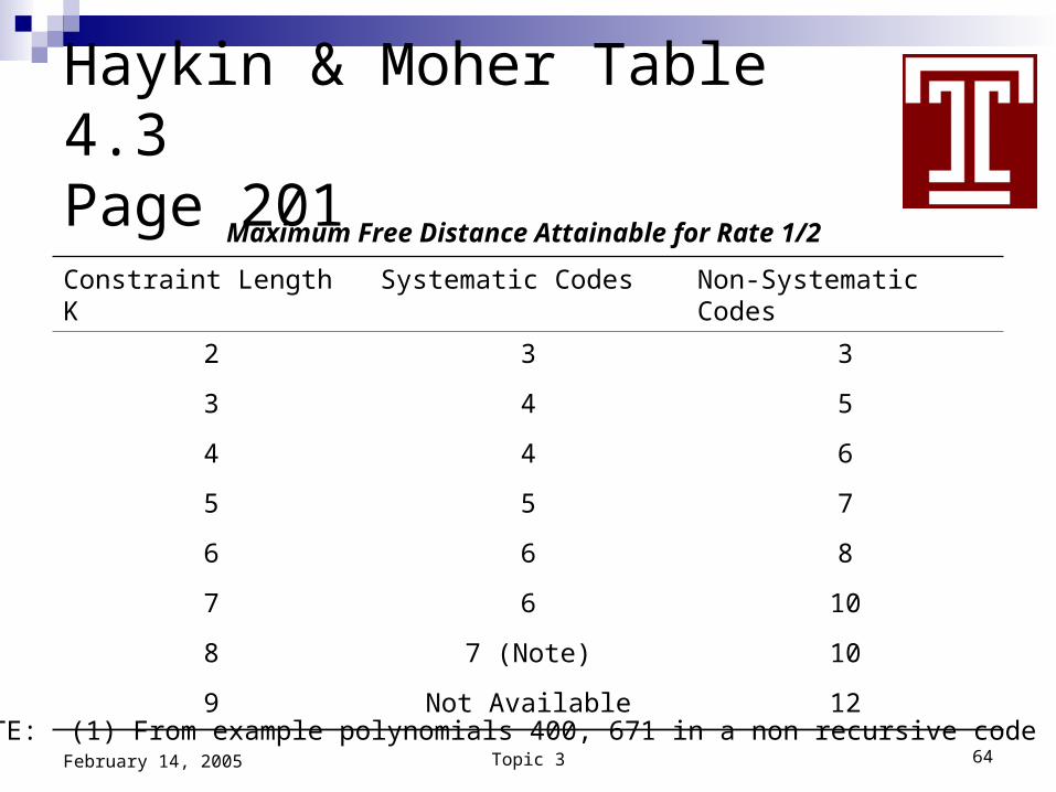
Haykin & Moher Table 4.3Page 201
Constraint Length K Systematic Codes Non-Systematic Codes
2 3 3
3 4 5
4 4 6
5 5 7
6 6 8
7 6 10
8 7 (Note) 10
9 Not Available 12
NOTE: (1) From example polynomials 400, 671 in a non recursive code
Maximum Free Distance Attainable for Rate 1/2
Topic 3 65February 14, 2005
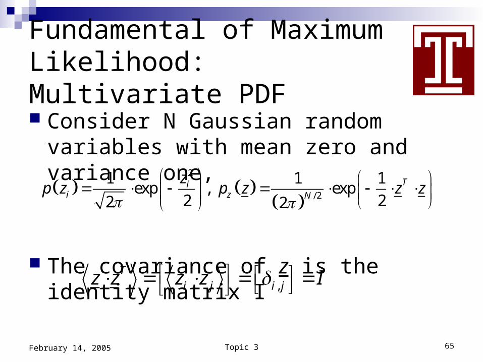
Fundamental of Maximum Likelihood: Multivariate PDF Consider N Gaussian random variables
with mean zero and variance one,
The covariance of z is the identity matrix I
2
/ 2
1 1 1exp , exp
2 22 2
Tii z N
zp z p z z z
,T
i j i jz z z z I
Topic 3 66February 14, 2005
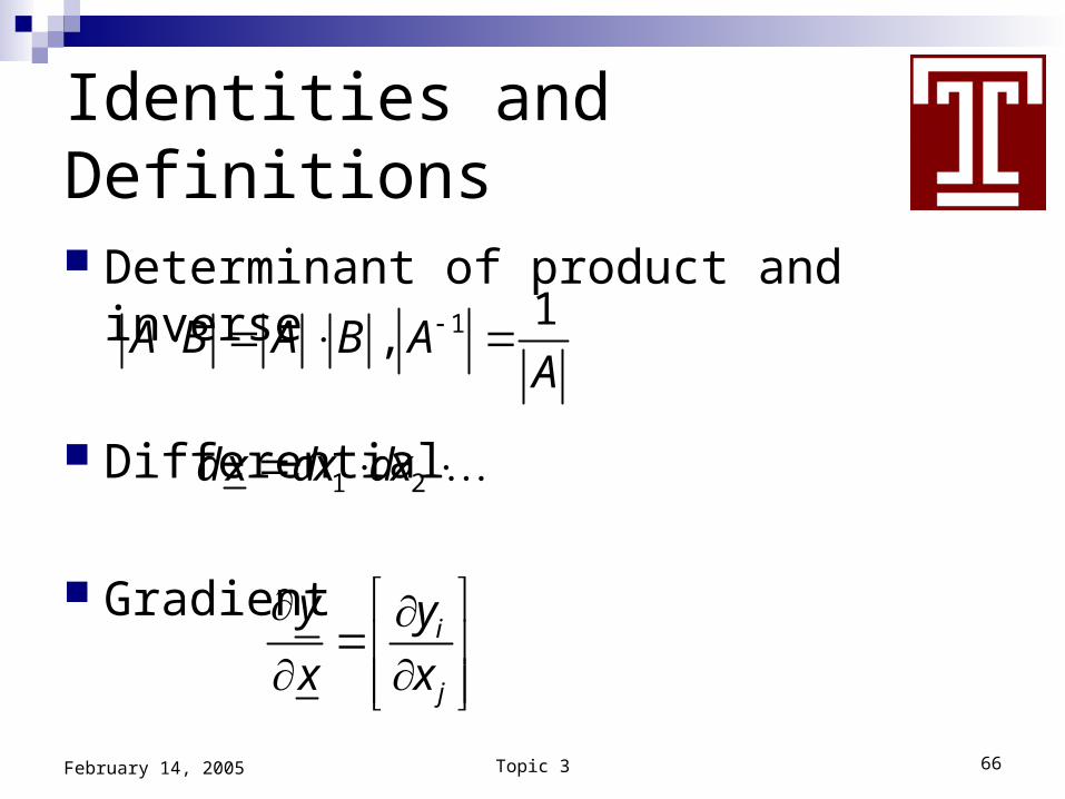
Identities and Definitions
Determinant of product and inverse
Differential
Gradient
1 1,A B A B A
A
1 2d x dx dx
i
j
y y
x x
Topic 3 67February 14, 2005
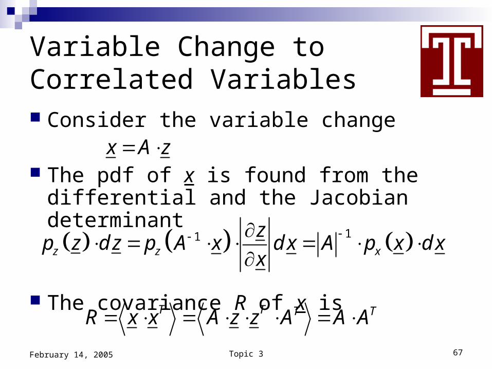
Variable Change to Correlated Variables Consider the variable change
The pdf of x is found from the differential and the Jacobian determinant
The covariance R of x is
x A z
T T T TR x x A z z A A A
11z z x
zp z d z p A x d x A p x d x
x
Topic 3 68February 14, 2005
PDF of Correlated Variables
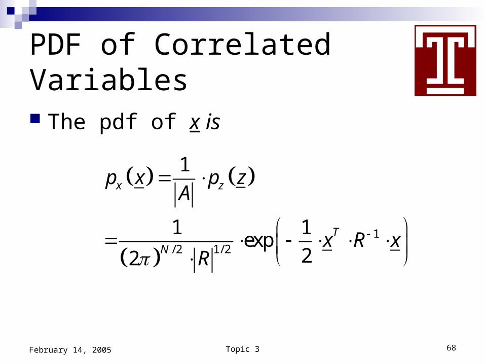
The pdf of x is
1
1/ 2/ 2
1
1 1exp
22
x z
T
N
p x p zA
x R xR
Topic 3 69February 14, 2005
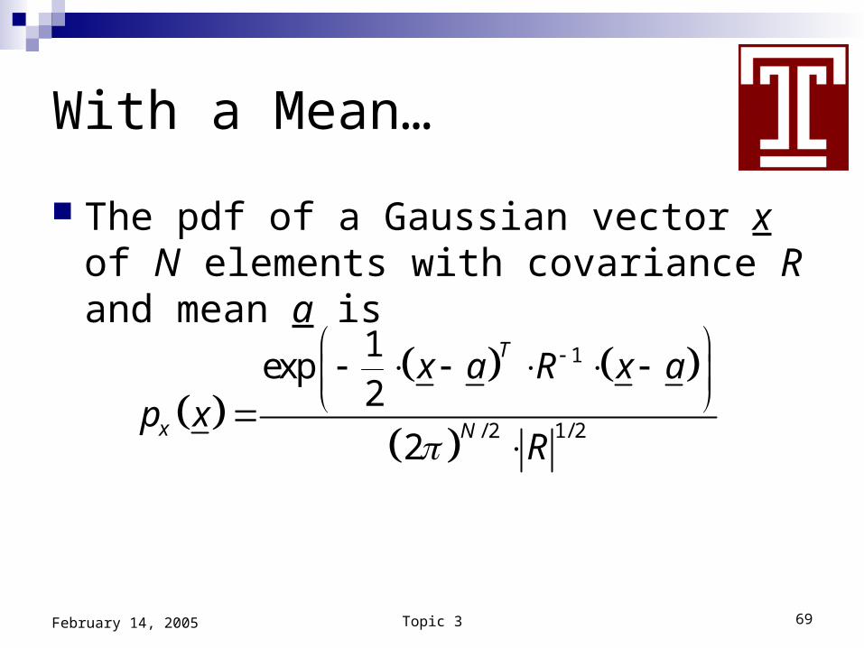
With a Mean…
The pdf of a Gaussian vector x of N elements with covariance R and mean a is
1
1/ 2/ 2
1exp
2
2
T
x N
x a R x ap x
R
Topic 3 70February 14, 2005
Maximum Likelihood Estimators
Principle Given the pdf of a data vector y as available, for a
given set of parameters x is p(y|x) Find the set of parameters x hat that maximizes this
pdf for the given set of measurements y Properties
If a minimum variance estimator exists, this method will produce it
If not, the variance will approach the theoretical minimum – the Cramer-Rao bound – as the amount of relevant data increases
Topic 3 71February 14, 2005
Observations on Maximum Likelihood All known minimum variance estimators can be
derived using the method of maximum likelihood; examples include Mean as average of samples Proportion in general population as proportion in a
sample Statistics and error bounds on estimators are
found as part of the derivation The method is simple to use
Topic 3 72February 14, 2005
Our Example
Given a message vector m and its code vector c and a received vector r
Make an estimate m hat of the message vector Process
With the noisy c through the receiver channel estimate c hat
Select the code m hat that produces a code vector c tilde has the shortest Hamming distance to c hat
Topic 3 73February 14, 2005
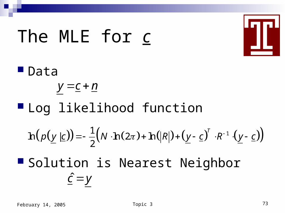
The MLE for c
Data
Log likelihood function
Solution is Nearest Neighbor
y c n
11ln | ln 2 ln
2
Tp y c N R y c R y c
c y
Topic 3 74February 14, 2005
Assignment
Read 4.7, 4.8, 4.10, 4.11, 4.16 Do problem 4.1 p. 197 Do problem 4.2 p. 198 Do encoding in your term project
Topic 3 75February 14, 2005
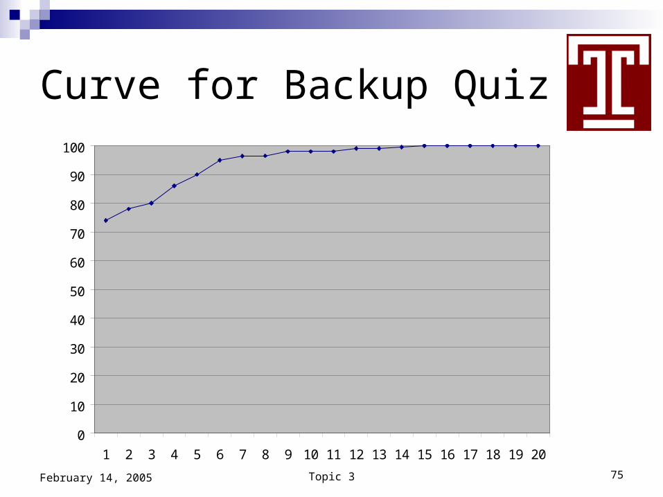
Curve for Backup Quiz
0
10
20
30
40
50
60
70
80
90
100
1 2 3 4 5 6 7 8 9 10 11 12 13 14 15 16 17 18 19 20
Topic 3 76February 14, 2005
Assignment
Read 5.2, 5.3, 5.5 Look at Problem 4.5 p. 243 Do problems 4.6, 4.7 p. 252
Topic 3 77February 14, 2005
Interleaving and TDMA
The Viterbi Method Interleaving
Scatters the code data streamMakes low BER communication more robust
through fading medium and interference Noise performance TDMA
Topic 3 78February 14, 2005
Viterbi Algorithm References
Viterbi, A.J., Error bounds for convolutional codes and an asymptotically optimum decoding algorithm, IEEE Trans. Inform. Theory, Vol. IT-13, pp. 260-269, 1967.
Forney, G.D. Jr. The Viterbi algorithm, Proceedings of the IEEE, Vol. 61, pp. 268-278, 1973.
Topic 3 79February 14, 2005
The Viterbi Method
Use the trellis for decoding Dynamic programming
A method originally developed for a control theory problem by Richard Bellman
Based on working the problem from the end back to the beginning
Uses the Hamming distance as an optimization criteria
Crops the growing decision tree by taking the steps backward in time a few at a time
Topic 3 80February 14, 2005
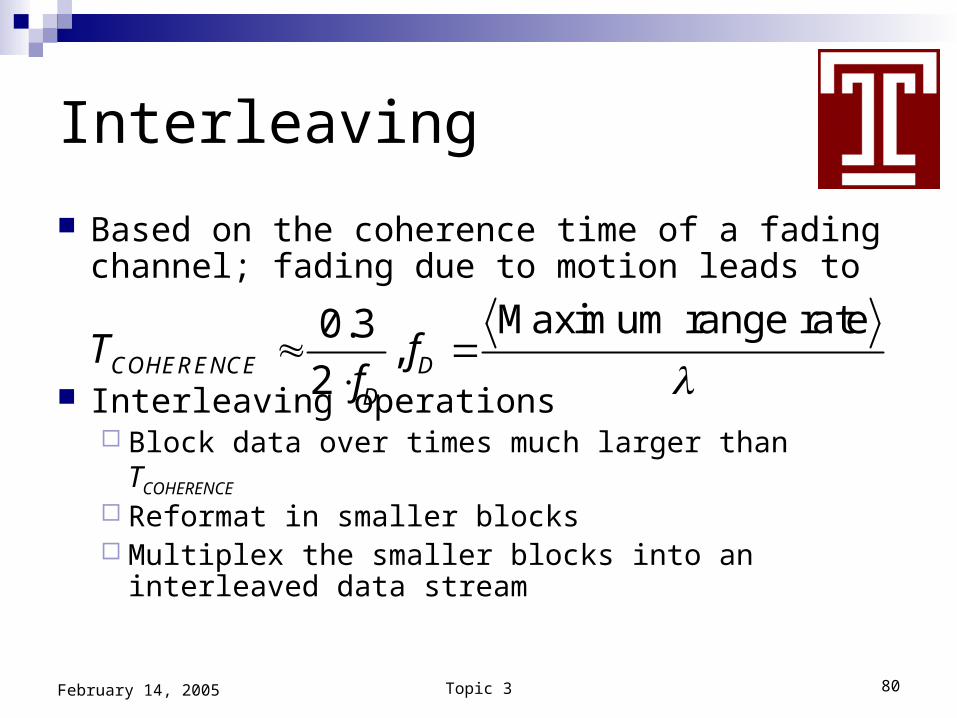
Interleaving
Based on the coherence time of a fading channel; fading due to motion leads to
Interleaving operations Block data over times much larger than TCOHERENCE
Reformat in smaller blocks Multiplex the smaller blocks into an interleaved data
stream
Maximum range rate0.3,
2COHERENCE DD
T ff
Topic 3 81February 14, 2005
Interleaver Parameters
Object of interleavingData blackouts of TCOHERENCE cause loss of less
than dfree bits
FEC EDAC coding can bridge these gaps Make each row
Consist of at least dfree bits
Last TCOHERENCE or longer
Topic 3 82February 14, 2005
Interleaver Methods
MethodsSimple sequential interleaving as just
describedPseudorandom interleaving
Combine with codesUse Viterbi interleaverUse multiplexer of convolutional codes as
interleaver
Topic 3 83February 14, 2005
Noise performance
Compare AWGN channels using Figure 4.13 p. 213
Rayleigh fading performance given in Figure 4.14 p. 214
Topic 3 84February 14, 2005
Turbo Codes
Revolutionary methodology Emerged in 1993 through 1995 Performance approaches Shannon limit
Technique Encoding blocked out in Figure 4.5 p. 215 Two systematic codes in parallel, one interleaved Excess parity bits trimmed or culled Decoding shown in Figure 4.17 p. 217
Performance shown in Figure 4.18 p. 219
Topic 3 85February 14, 2005
Next Time
TDMA Chapter 4 examples Quiz postponed one week to March 30
Will cover Chapter 4Some topics in CDMA
Topic 3 86February 14, 2005
TDMA
Time-Division Multiple Access (TDMA) Multiplex several users into one channel Alternative to FDMA Third alternative is CDMA, presented next
Advantages over FDMA Simultaneous transmit and receive aren’t required Single-frequency operation for transmit and receive Can be combined with interleaving Can be overlaid on FDMA, CDMA
Topic 3 87February 14, 2005
Types of TDMA
Wideband Used in links such as satellite communications Frequency channels several MHz wide
Medium band Global System for Mobile (GSM) telecommunications Several broadband links
Narrow band TIA/EIA/IS-54-C standard in use for US cell phones Single frequency channel TDMA
Topic 3 88February 14, 2005
Advantages of TDMA overlaying FDMA Cooperative channel allocation between
base stations with overlapping coverage (channel-busy avoidance)
Dropouts in some channels from frequency-dependent fading can be avoided
Equalization can mitigate frequency-dependent fading in medium and broad band TDMA/FDMA
Topic 3 89February 14, 2005
Global System for Mobile (GSM) Internationally used TDMA/FDMA From Haykin & Moher 4.17 pp. 236-239 Overview given here Full description available on WWW
http://ccnga.uwaterloo.ca/~jscouria/GSM/gsmreport.html Organization
Time blocks Major frames are 60/13 = 4.615 milliseconds Eight Time Slots of 577 microseconds in each major frame 156.25 bits per time slot; 271 kBPS data rate
Frequency channels 124 channels 200 kHz wide, 200 kHz apart Frequency hopping with maximum of 25 MHz
Topic 3 90February 14, 2005
GSM Characteristics
Frequency allocation (Europe) Uplink (to base station) 890 MHz to 915 MHz Downlink (to handsets) 935 MHz to 960 MHz
Design features counter frequency-selective fade Channel separation matches fading notch width Frame length matches fading duration EDAC combined with multilayer interleaving
Intrinsic latency is 57.5 milliseconds
Topic 3 91February 14, 2005
Subframe Organization
Guard period of 8.25 bits begins the frame Three tail bits end guard and time slots Three data blocks
57 bits of data 26 bits of “training data” 57 bits of data
Flag bit precedes training and second data block Defines speech vs. digital or training data
Overall efficiency about 75% data
Topic 3 92February 14, 2005
GSM Coding
Complex speech coder/decoder (CODEC) Concatenated convolutional codes Multi-layer interleaving GMSK channel modulation
About 40 dB adjacent channel rejection ISI effects are small
An international standard that defines affordable enabling technologies
Topic 3 93February 14, 2005
Coherence Time Examples
Mobile terminal moving at 30 km/hr (19 mph) Frequency allocation about 1.9 GHz
Problem 4.4 p. 210 answer is 9.6 ms (!!!) Coherence time about 2.84 ms
Frequency of about 900 MHz European GSM allocation Coherence time of about 6 ms Velocity of 39 km/hr (24 mph) gives coherence time of
4.62 ms frame time
Topic 3 94February 14, 2005
Problems 4.6, 4.7
Message is 10111… (1’s continue) Codes are (see p. 253)
Problem 4.6: (11)(10)Problem 4.7: (1111)(1101)
Find output code stream by polynomial method
Topic 3 95February 14, 2005
Solution for Problem 4.6
Solution is simple enough to do by inspection:(11,10,11,01,01,01,…)Feed-through path embeds signal in the codeThis makes the code systematic
Topic 3 96February 14, 2005
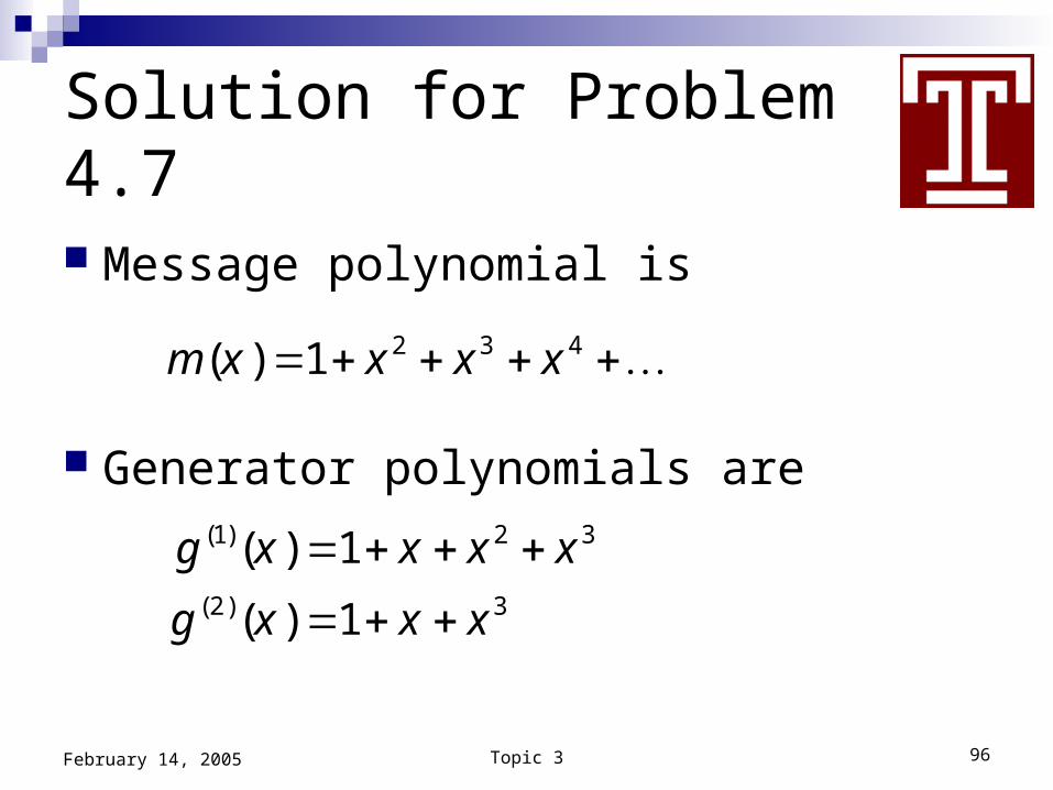
Solution for Problem 4.7
Message polynomial is
Generator polynomials are
2 3 4( ) 1m x x x x
(1) 2 3
(2) 3
( ) 1
( ) 1
g x x x x
g x x x
Topic 3 97February 14, 2005
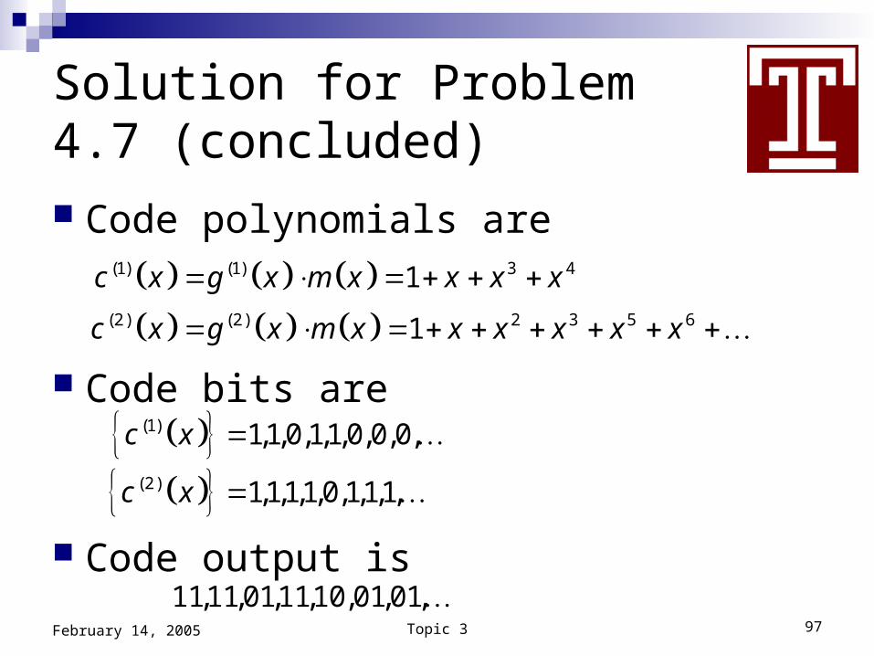
Solution for Problem 4.7 (concluded) Code polynomials are
Code bits are
Code output is
(1) (1) 3 4
(2) (2) 2 3 5 6
1
1
c x g x m x x x x
c x g x m x x x x x x
(1)
(2)
1,1,0,1,1,0,0,0,
1,1,1,1,0,1,1,1,
c x
c x
11,11,01,11,10,01,01,
Topic 3 98February 14, 2005
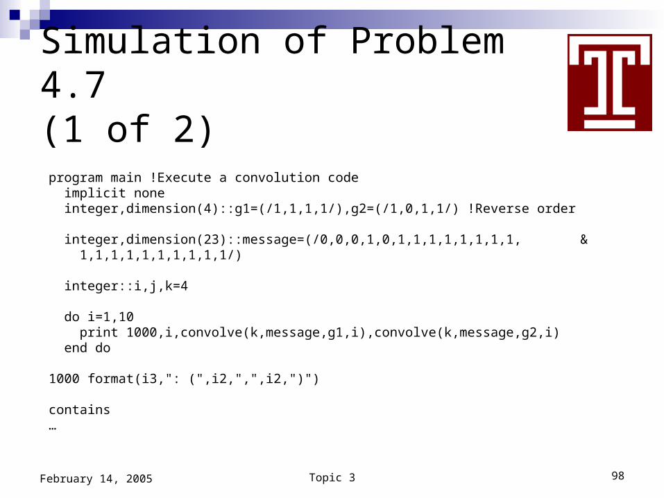
Simulation of Problem 4.7(1 of 2)
program main !Execute a convolution code implicit none integer,dimension(4)::g1=(/1,1,1,1/),g2=(/1,0,1,1/) !Reverse order
integer,dimension(23)::message=(/0,0,0,1,0,1,1,1,1,1,1,1,1, & 1,1,1,1,1,1,1,1,1,1/)
integer::i,j,k=4
do i=1,10 print 1000,i,convolve(k,message,g1,i),convolve(k,message,g2,i) end do
1000 format(i3,": (",i2,",",i2,")")
contains…
Topic 3 99February 14, 2005
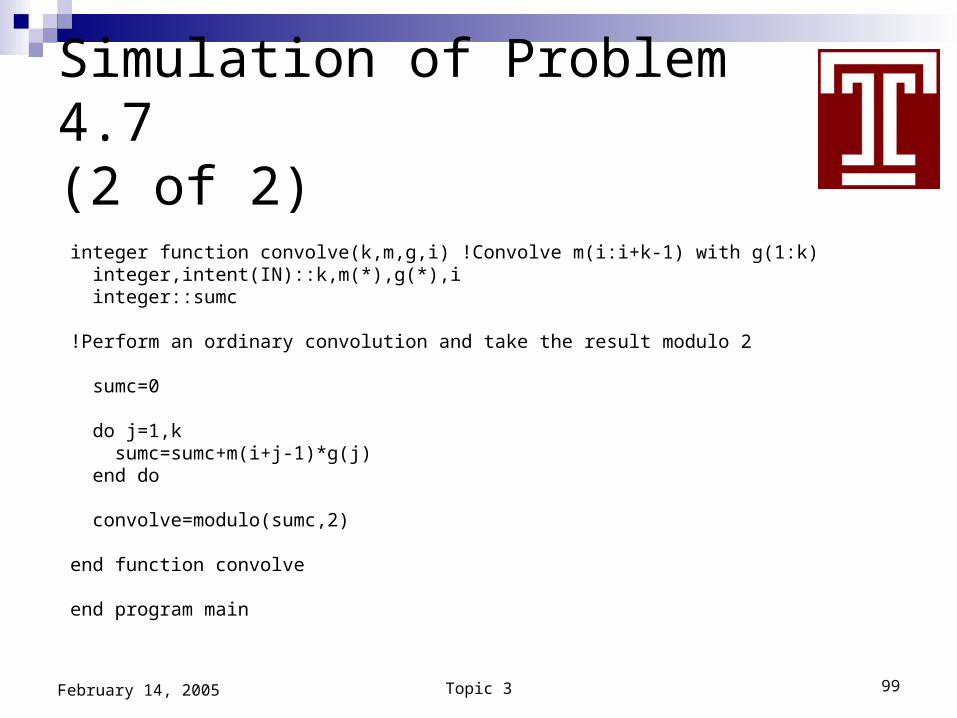
Simulation of Problem 4.7(2 of 2)
integer function convolve(k,m,g,i) !Convolve m(i:i+k-1) with g(1:k) integer,intent(IN)::k,m(*),g(*),i integer::sumc
!Perform an ordinary convolution and take the result modulo 2
sumc=0
do j=1,k sumc=sumc+m(i+j-1)*g(j) end do
convolve=modulo(sumc,2)
end function convolve
end program main
Topic 3 100February 14, 2005
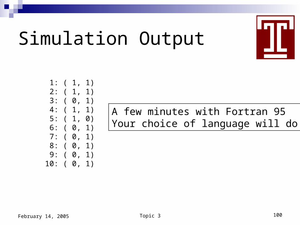
Simulation Output
1: ( 1, 1) 2: ( 1, 1) 3: ( 0, 1) 4: ( 1, 1) 5: ( 1, 0) 6: ( 0, 1) 7: ( 0, 1) 8: ( 0, 1) 9: ( 0, 1) 10: ( 0, 1)
A few minutes with Fortran 95Your choice of language will do.
Topic 3 101February 14, 2005
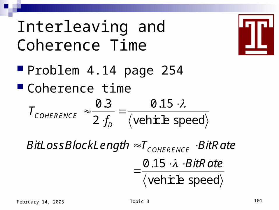
Interleaving and Coherence Time Problem 4.14 page 254 Coherence time
0.3 0.15
2 vehicle speedCOHERENCED
Tf
0.15
vehicle speed
COHERENCEBitLossBlockLength T BitRate
BitRate
Topic 3 102February 14, 2005
Discussion Questions
One-Channel TDMAWhat about both transmit and receive on the
same frequency channel? Is it a good idea? Why?
What are the advantages and disadvantages of systematic and non-systematic codes?
Topic 3 103February 14, 2005
Assignment
Read 5.2, 5.3, 5.5 Look at problem 5.1 p. 262 Do problem 5.2 p. 263 Next time
Spreading the spectrumGold codesGalois fields for binary sequences