Embed Size (px)
Citation preview
||
Göran AnderssonPower System Laboratory, ETH Zürich
Felix Wu Distinguished Lecture in Power SystemsThe University of Hong Kong, 10th November 2014
The Future Electric Power SystemDevelopments and New Analysis Tools
||
Outline
• Power System Lab (PSL), ETH Zurich
• New Challenges and Recent Developments
• Power Node Modeling Framework
• Cyber- security in Power Systems
• Concluding Remarks
2
||
PSL Research (and Teaching)
• Power System Operation and Control
• Power Markets
• Future Energy Systems
Main Methods & Tools used• Control theory• Optimization• Simulation• ...
3
||
The PSL Team
4
||
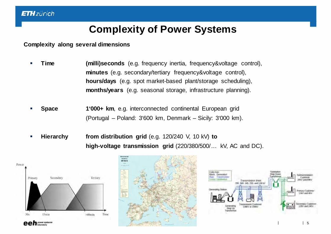
Complexity of Power SystemsComplexity along several dimensions
Time (milli)seconds (e.g. frequency inertia, frequency&voltage control),minutes (e.g. secondary/tertiary frequency&voltage control),hours/days (e.g. spot market-based plant/storage scheduling),months/years (e.g. seasonal storage, infrastructure planning).
Space 1‘000+ km, e.g. interconnected continental European grid(Portugal – Poland: 3‘600 km, Denmark – Sicily: 3‘000 km).
Hierarchy from distribution grid (e.g. 120/240 V, 10 kV) tohigh-voltage transmission grid (220/380/500/… kV, AC and DC).
5
||
49.88
49.89
49.90
49.91
49.92
49.93
49.94
49.95
49.96
49.97
49.98
49.99
50.00
50.01
50.02
16:45:00 16:50:00 16:55:00 17:00:00 17:05:00 17:10:00 17:15:00
8. Dezember 2004
f [Hz]
49.88
49.89
49.90
49.91
49.92
49.93
49.94
49.95
49.96
49.97
49.98
49.99
50.00
50.01
50.02
16:45:00 16:50:00 16:55:00 17:00:00 17:05:00 17:10:00 17:15:00
8. Dezember 2004
f [Hz]
Frequency Athens
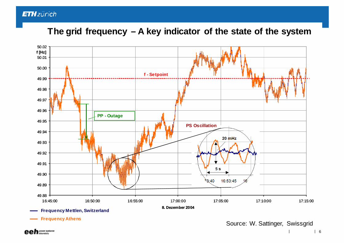
The grid frequency – A key indicator of the state of the system
f - Setpoint
Frequency Mettlen, Switzerland
PP - Outage
PS Oscillation
Source: W. Sattinger, Swissgrid6
||
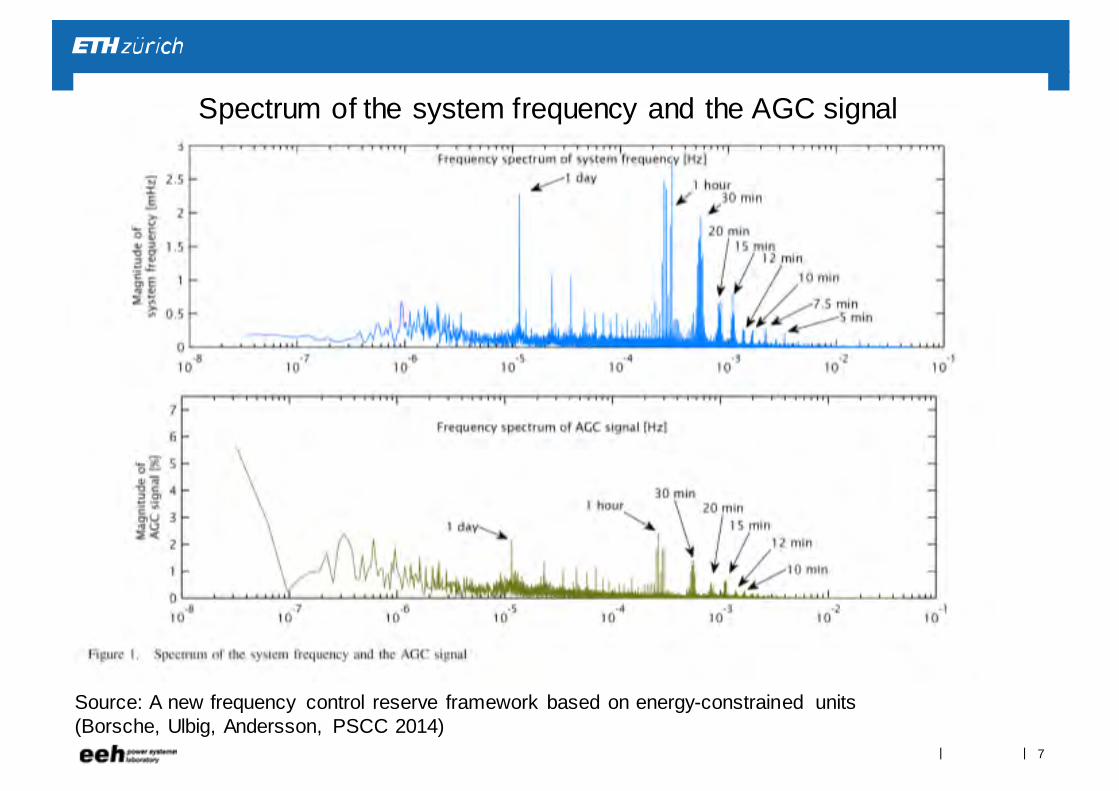
Source: A new frequency control reserve framework based on energy-constrained units (Borsche, Ulbig, Andersson, PSCC 2014)
Spectrum of the system frequency and the AGC signal
7
||
Power Flow
Control(e.g. line
switching)
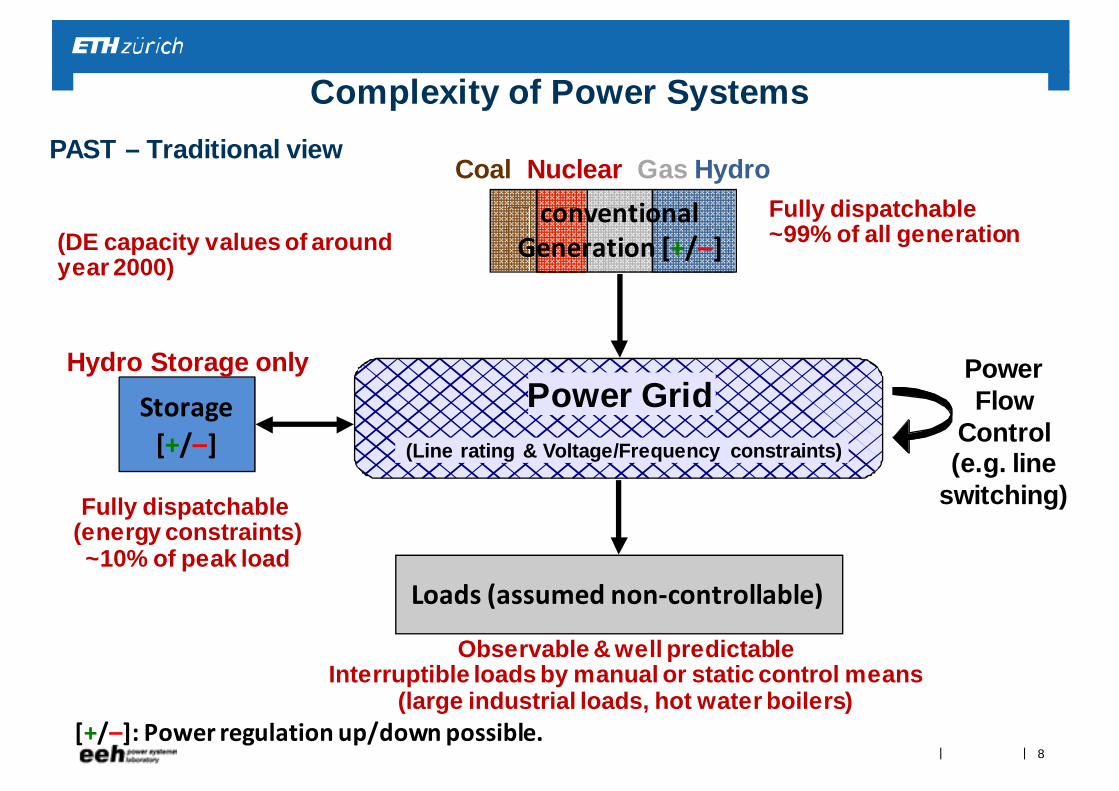
PAST – Traditional view
Storage[+/–]
Loads (assumed non‐controllable)
Power Grid(Line rating & Voltage/Frequency constraints)
[+/–]: Power regulation up/down possible.
Coal Nuclear Gas Hydroconventional
Generation [+/–]
Complexity of Power Systems
(DE capacity values of aroundyear 2000)
Fully dispatchable~99% of all generation
Hydro Storage only
Fully dispatchable (energy constraints)~10% of peak load
Observable & well predictableInterruptible loads by manual or static control means
(large industrial loads, hot water boilers)
8
||
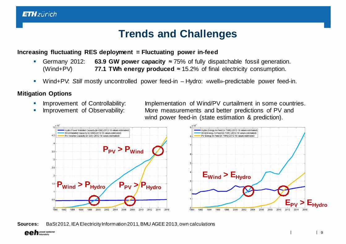
Increasing fluctuating RES deployment = Fluctuating power in-feed Germany 2012: 63.9 GW power capacity ≈ 75% of fully dispatchable fossil generation.
(Wind+PV) 77.1 TWh energy produced ≈ 15.2% of final electricity consumption.
Wind+PV: Still mostly uncontrolled power feed-in – Hydro: «well»-predictable power feed-in.
Mitigation Options Improvement of Controllability: Implementation of Wind/PV curtailment in some countries. Improvement of Observability: More measurements and better predictions of PV and
wind power feed-in (state estimation & prediction).
Sources: BaSt2012, IEA ElectricityInformation 2011, BMU AGEE 2013, own calculations
PPV > PWind
PWind > PHydro
EWind > EHydroPPV > PHydro
EPV > EHydro
Trends and Challenges
9
||
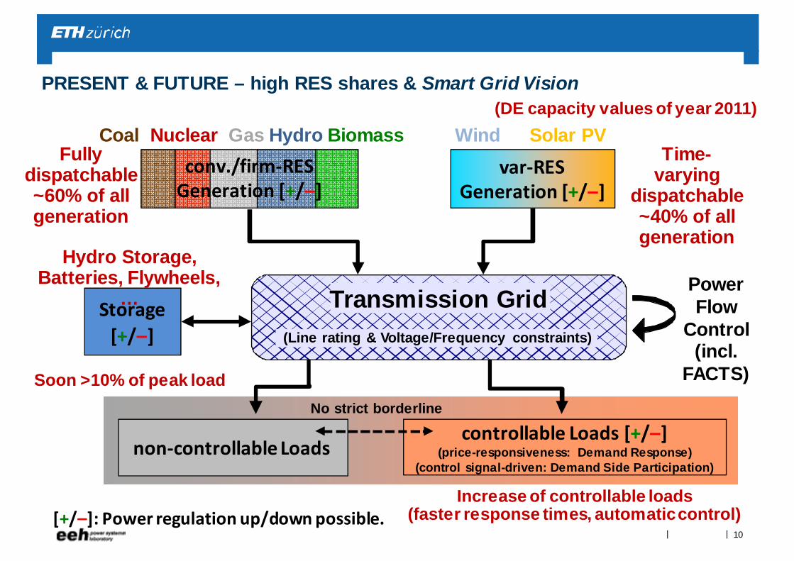
Transmission Grid
[+/–]: Power regulation up/down possible.
Storage[+/–] (Line rating & Voltage/Frequency constraints)
var‐RESGeneration [+/–]
Coal Nuclear Gas Hydro Biomass Wind Solar PVconv./firm‐RESGeneration [+/–]
Power Flow
Control(incl.
FACTS)
controllable Loads [+/–](price-responsiveness: Demand Response)
(control signal-driven: Demand Side Participation)non‐controllable Loads
No strict borderline
PRESENT & FUTURE – high RES shares & Smart Grid Vision (DE capacity values of year 2011)
Time-varying
dispatchable~40% of all generation
Hydro Storage, Batteries, Flywheels,
…
Soon >10% of peak load
Increase of controllable loads(faster response times, automaticcontrol)
Fully dispatchable~60% of all generation
10
||
Power Nodes Framework
Kai Heussen (DTU)Stephan KochAndreas Ulbig...
11
||
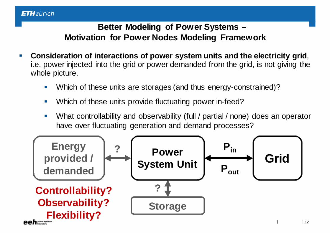
Consideration of interactions of power system units and the electricity grid, i.e. power injected into the grid or power demanded from the grid, is not giving the whole picture.
Which of these units are storages (and thus energy-constrained)?
Which of these units provide fluctuating power in-feed?
What controllability and observability (full / partial / none) does an operatorhave over fluctuating generation and demand processes?
Better Modeling of Power Systems –Motivation for Power Nodes Modeling Framework
Energy provided / demanded
Storage
?
?Controllability?Observability?
Flexibility?
GridPin
Pout
Power System Unit
12
||
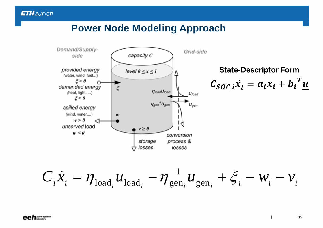
Power Node Modeling Approach
1load load gen geni i i ii i i i iC x u u w v
,
State-Descriptor Form
13
||
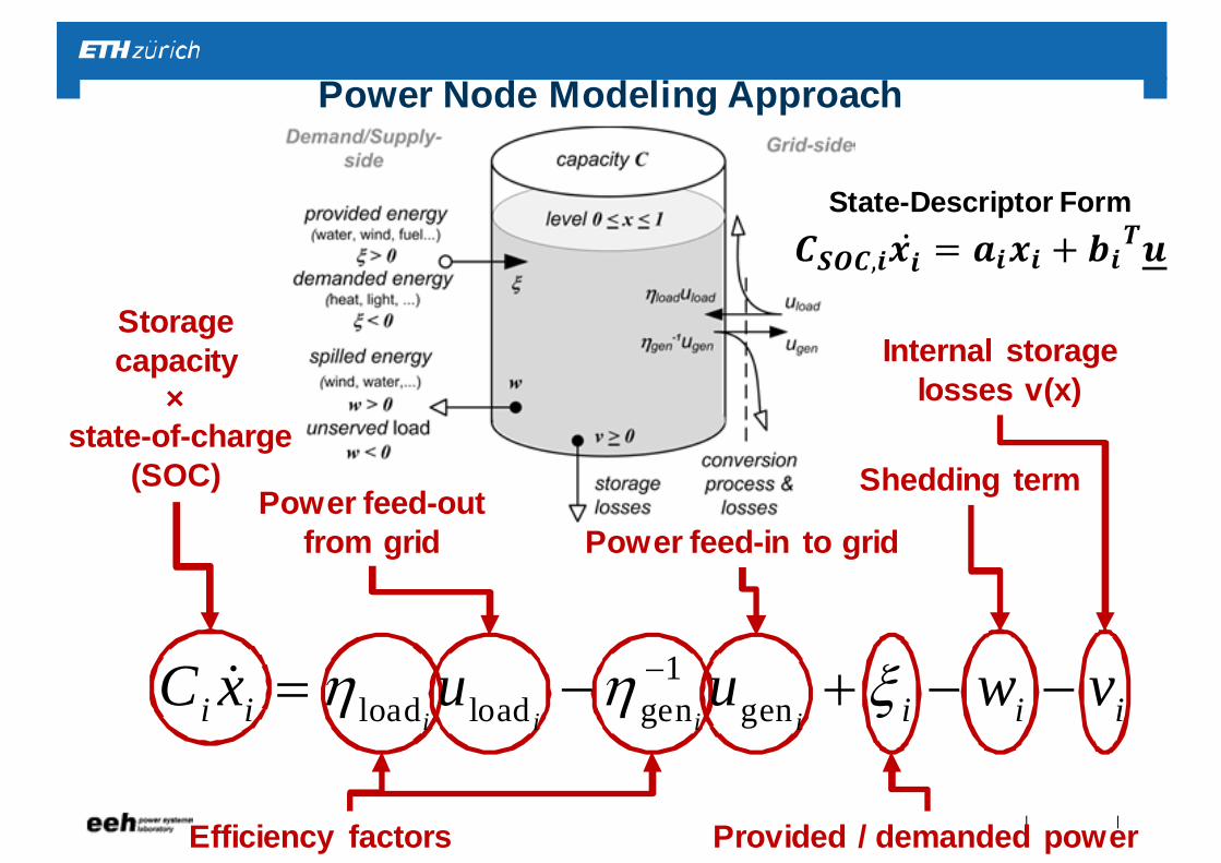
Power Node Modeling Approach
Power feed-in to grid
Efficiency factors
Storage capacity
×state-of-charge
(SOC)
Provided / demanded power
Shedding term
Internal storagelosses v(x)
Power feed-out from grid
1load load gen geni i i ii i i i iC x u u w v
,
State-Descriptor Form
||
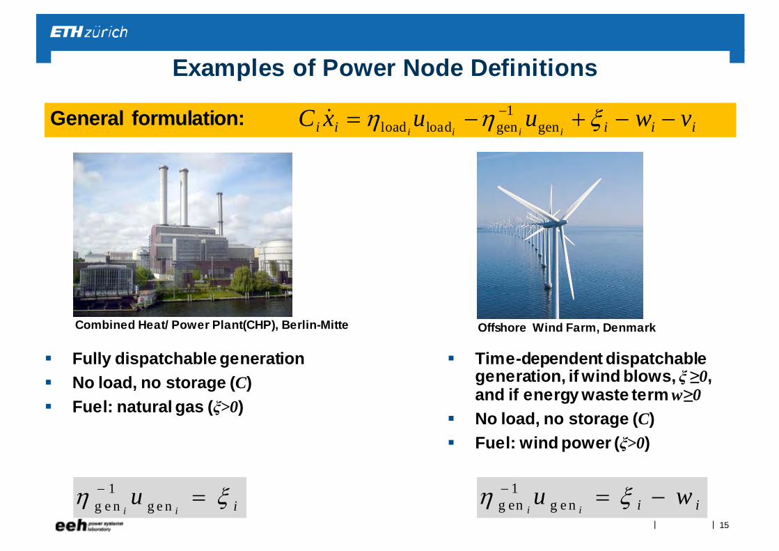
Examples of Power Node Definitions
Fully dispatchable generation No load, no storage (C) Fuel: natural gas (ξ>0)
Combined Heat/ Power Plant(CHP), Berlin-Mitte Offshore Wind Farm, Denmark
Time-dependent dispatchable generation, if wind blows, ξ ≥0, and if energy waste term w≥0
No load, no storage (C) Fuel: wind power (ξ>0)
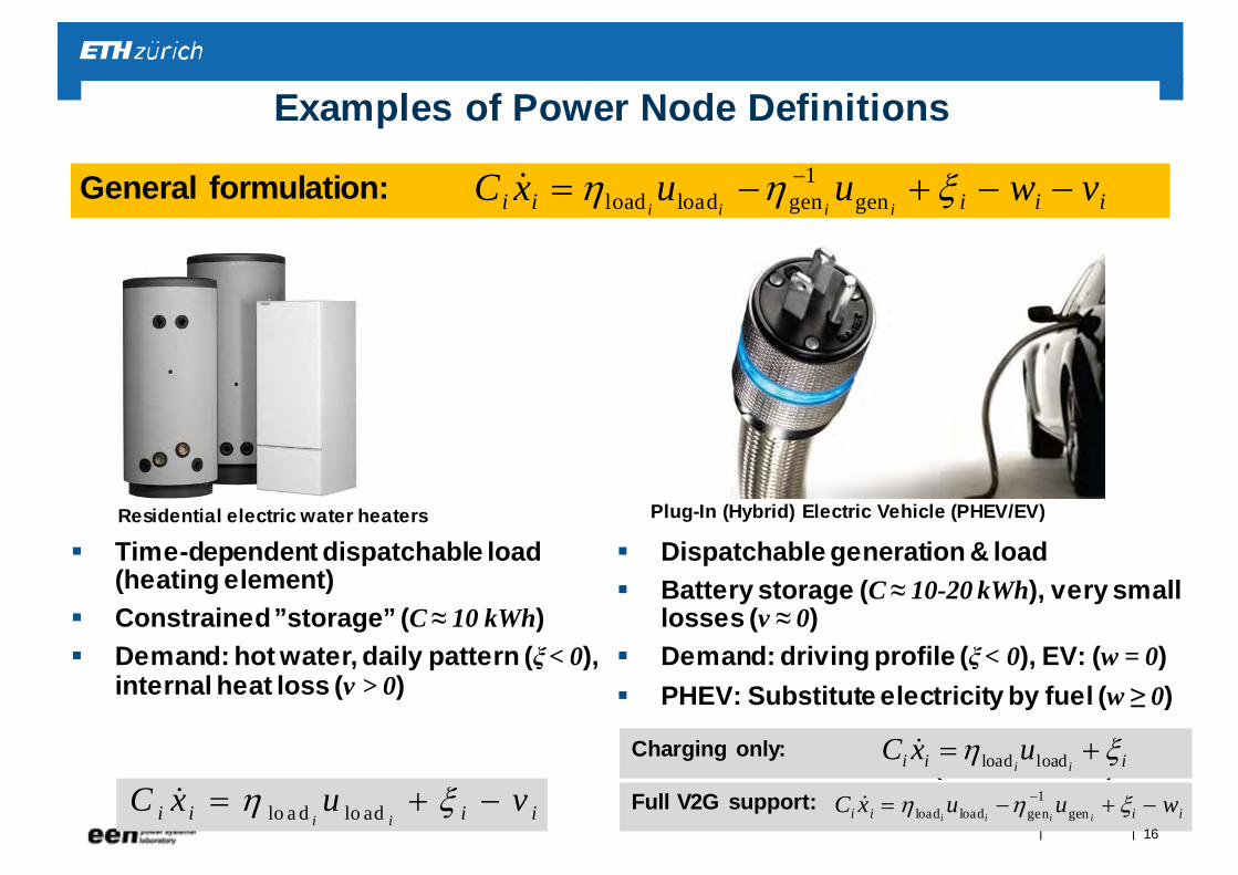
General formulation: 1load load gen geni i i ii i i i iC x u u w v
1g en g e ni i i iu w 1
g e n g e ni i iu 15
||
Examples of Power Node Definitions
Time-dependent dispatchable load (heating element)
Constrained ”storage” (C ≈ 10 kWh) Demand: hot water, daily pattern (ξ< 0),
internal heat loss (v > 0)
Residential electric water heaters
Emosson (Nant de Drance)
Dispatchable generation & load Battery storage (C ≈ 10-20 kWh), very small
losses (v ≈ 0) Demand: driving profile (ξ< 0), EV: (w = 0) PHEV: Substitute electricity by fuel (w ≥ 0)
Plug-In (Hybrid) Electric Vehicle (PHEV/EV)
Charging only:
Full V2G support:
General formulation: 1load load gen geni i i ii i i i iC x u u w v
lo a d lo adi ii i i iC x u v load loadi ii i iC x u
1load load gen geni i i ii i i iC x u u w
16
||
Examples of Power Node Definitions
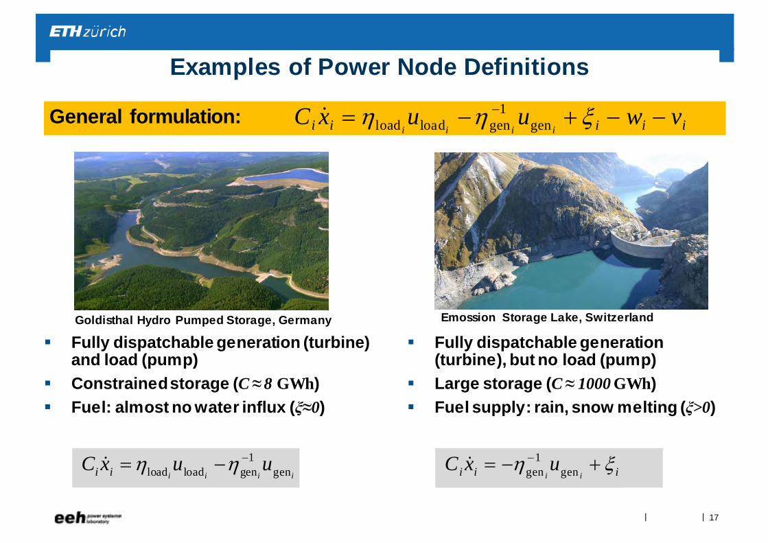
Fully dispatchable generation (turbine) and load (pump)
Constrained storage (C ≈ 8 GWh) Fuel: almost no water influx (ξ≈0)
Goldisthal Hydro Pumped Storage, Germany
Fully dispatchable generation (turbine), but no load (pump)
Large storage (C ≈ 1000 GWh) Fuel supply: rain, snow melting (ξ>0)
Emossion Storage Lake, Switzerland
General formulation: 1load load gen geni i i ii i i i iC x u u w v
1gen geni ii i iC x u 1
load load gen geni i i ii iC x u u
17
||
Examples of Power Node Definitions
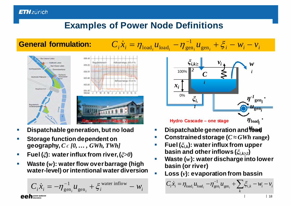
1 water inflowgen geni ii i i iC x u w
Dispatchable generation and load Constrained storage (C ≈ GWh range) Fuel (ξi,k): water influx from upper
basin and other inflows (ξi,k≥2) Waste (w): water discharge into lower
basin (or river) Loss (v): evaporation from bassin
Dispatchable generation, but no load Storage function dependent on
geography, C ϵ [0, … , GWh, TWh] Fuel (ξ): water influx from river, (ξ>0) Waste (w): water flow over barrage (high
water-level) or intentional water diversion
Run-of-River Plant, Zurich
1load load gen gen ,i i i ii i i k i i
k
C x u u w v
General formulation: 1load load gen geni i i ii i i i iC x u u w v
0%
100%
xi
Ci
vi wi
ξi,1
η-1geni
· ugeni
ηloadi·
uloadi
Hydro Cascade – one stage
ξi,k≥2
18
||
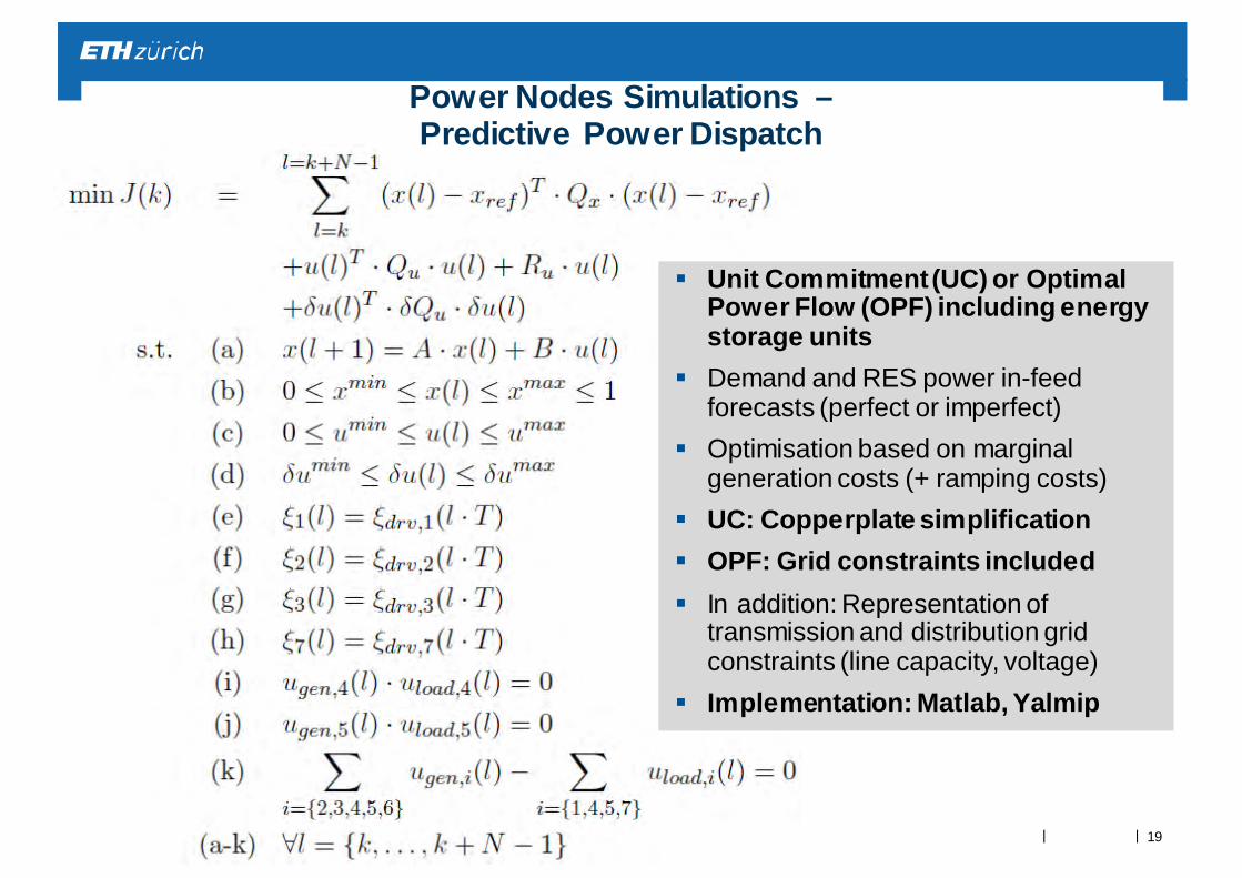
Unit Commitment (UC) or Optimal Power Flow (OPF) including energy storage units
Demand and RES power in-feed forecasts (perfect or imperfect)
Optimisation based on marginal generation costs (+ ramping costs)
UC: Copperplate simplification OPF: Grid constraints included In addition: Representation of
transmission and distribution grid constraints (line capacity, voltage)
Implementation: Matlab, Yalmip
Power Nodes Simulations –Predictive Power Dispatch
19
||
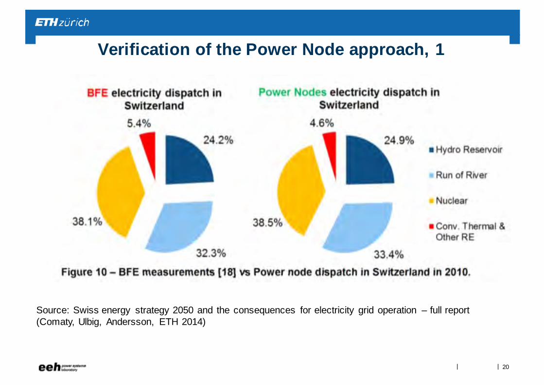
Source: Swiss energy strategy 2050 and the consequences for electricity grid operation – full report (Comaty, Ulbig, Andersson, ETH 2014)
Verification of the Power Node approach, 1
20
||
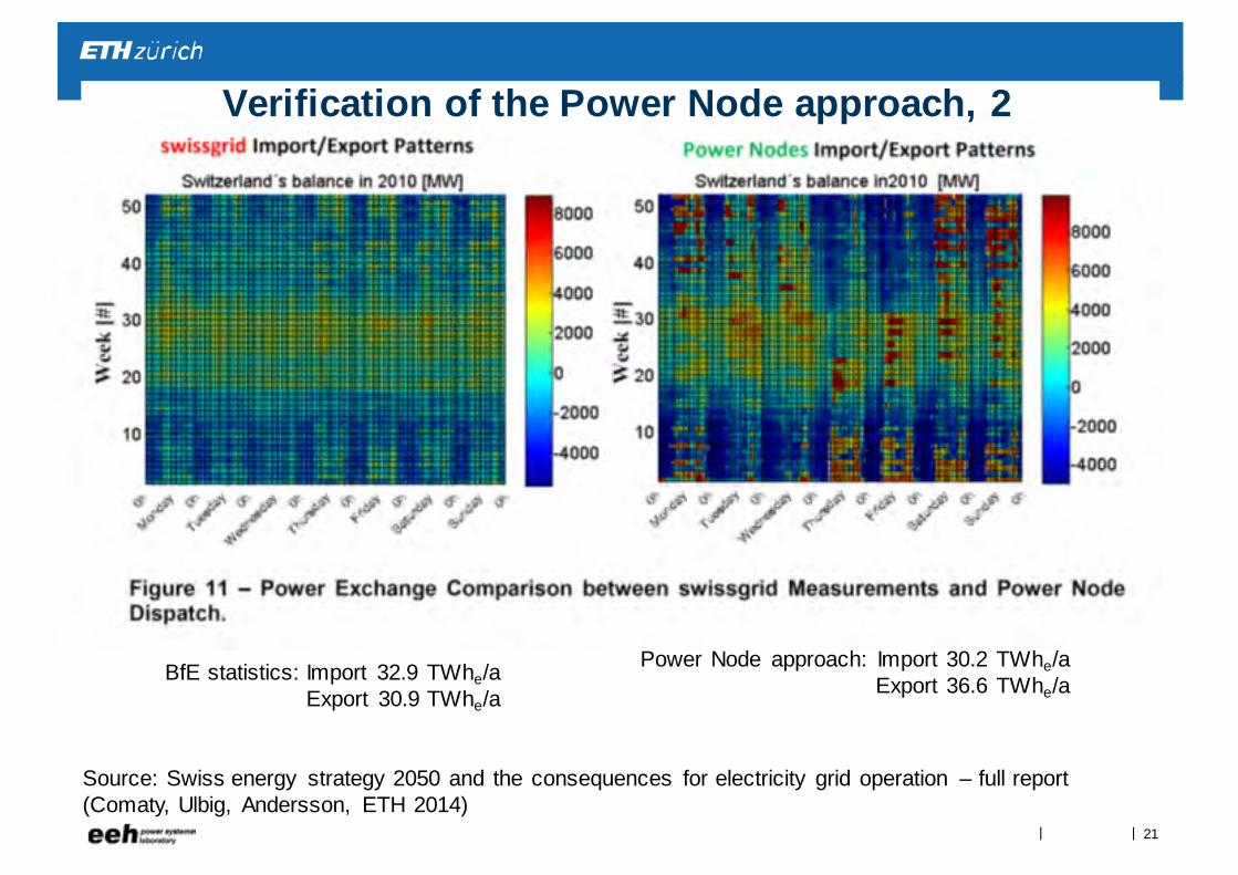
Verification of the Power Node approach, 2
Source: Swiss energy strategy 2050 and the consequences for electricity grid operation – full report (Comaty, Ulbig, Andersson, ETH 2014)
BfE statistics: Import 32.9 TWhe/aExport 30.9 TWhe/a
Power Node approach: Import 30.2 TWhe/aExport 36.6 TWhe/a
21
||
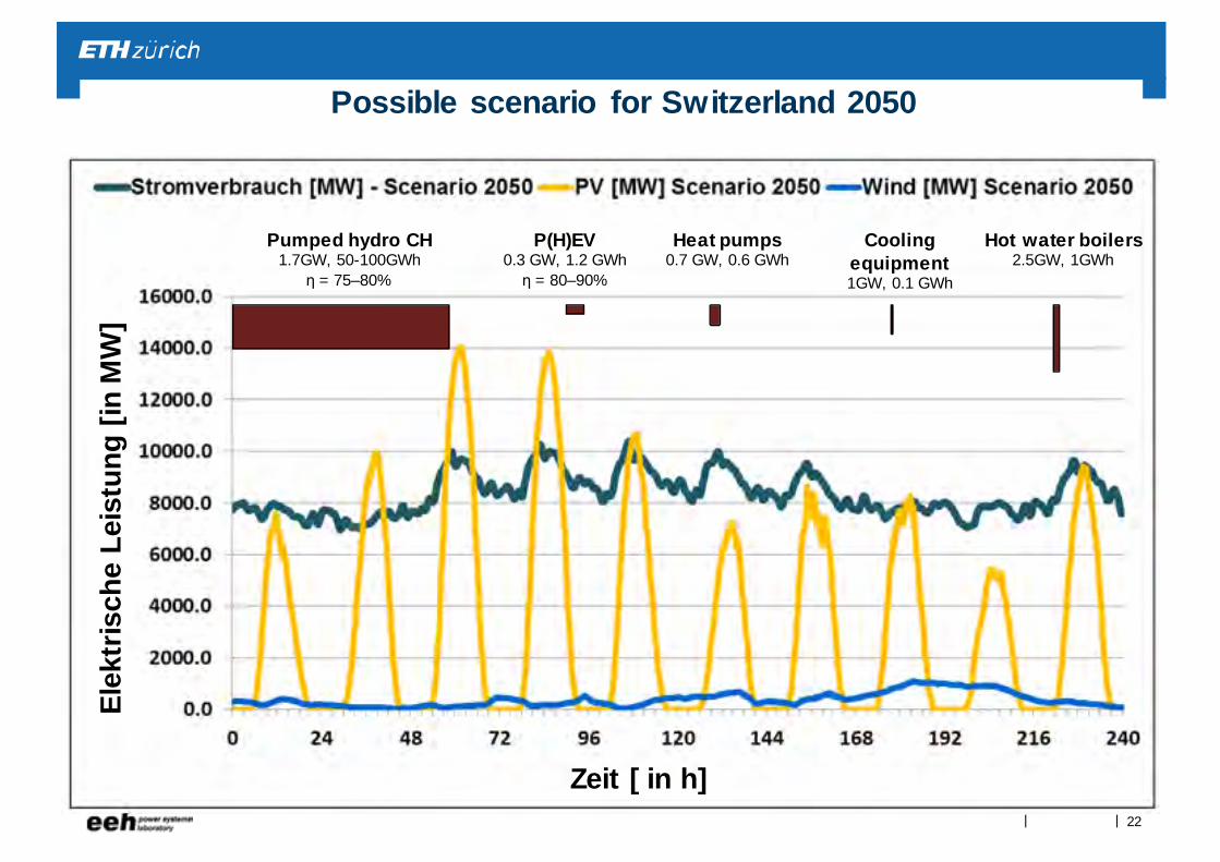
Possible scenario for Switzerland 2050
Zeit [ in h]
Elek
tris
che
Leis
tung
[in
MW
]
Pumped hydro CH1.7GW, 50-100GWh
η = 75–80%
Heat pumps0.7 GW, 0.6 GWh
Coolingequipment1GW, 0.1 GWh
Hot water boilers2.5GW, 1GWh
P(H)EV0.3 GW, 1.2 GWh
η = 80–90%
22
||
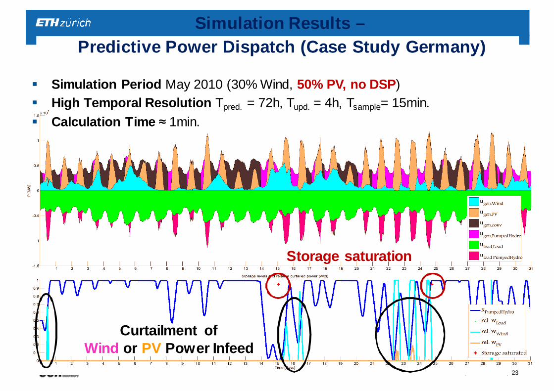
Storage saturation
Curtailment ofWind or PV Power Infeed
Simulation Period May 2010 (30% Wind, 50% PV, no DSP) High Temporal Resolution Tpred. = 72h, Tupd. = 4h, Tsample= 15min. Calculation Time ≈ 1min.
Simulation Results –Predictive Power Dispatch (Case Study Germany)
23
||
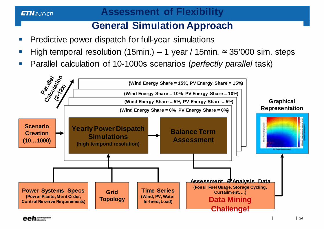
Assessment of FlexibilityGeneral Simulation Approach
(Wind Energy Share = 15%, PV Energy Share = 15%)
(Wind Energy Share = 10%, PV Energy Share = 10%)
(Wind Energy Share = 5%, PV Energy Share = 5%)
(Wind Energy Share = 0%, PV Energy Share = 0%)
Scenario Creation
(10…1000)
Yearly Power Dispatch Simulations
(high temporal resolution)
Balance Term Assessment
GridTopology
Time Series(Wind, PV, Water
In-feed, Load)
Power Systems Specs(Power Plants, Merit Order,
Control Reserve Requirements)
Assessment & Analysis Data(Fossil Fuel Usage, Storage Cycling,
Curtailment, …)
Data Mining Challenge!
GraphicalRepresentation
Predictive power dispatch for full-year simulations High temporal resolution (15min.) – 1 year / 15min. ≈ 35’000 sim. steps Parallel calculation of 10-1000s scenarios (perfectly parallel task)
24
||
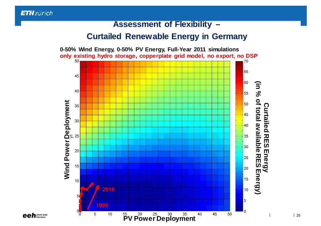
Assessment of Flexibility –Curtailed Renewable Energy in Germany
PV Power Deployment
Win
d Po
wer
Dep
loym
ent C
urtailedR
ES Energy(in %
oftotal availableR
ES Energy)
0-50% Wind Energy, 0-50% PV Energy, Full-Year 2011 simulationsonly existing hydro storage, copperplate grid model, no export, no DSP
25
||
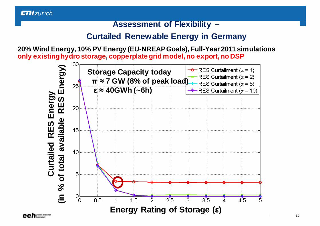
20% Wind Energy, 10% PV Energy (EU-NREAP Goals), Full-Year 2011 simulations only existing hydro storage, copperplate grid model, no export, no DSP
Cur
taile
dR
ES E
nerg
y(in
% o
ftot
al a
vaila
ble
RES
Ene
rgy)
Energy Rating of Storage (ε)
Storage Capacity todayπ ≈ 7 GW (8% of peak load)ε ≈ 40GWh (~6h)
Assessment of Flexibility –Curtailed Renewable Energy in Germany
26
||
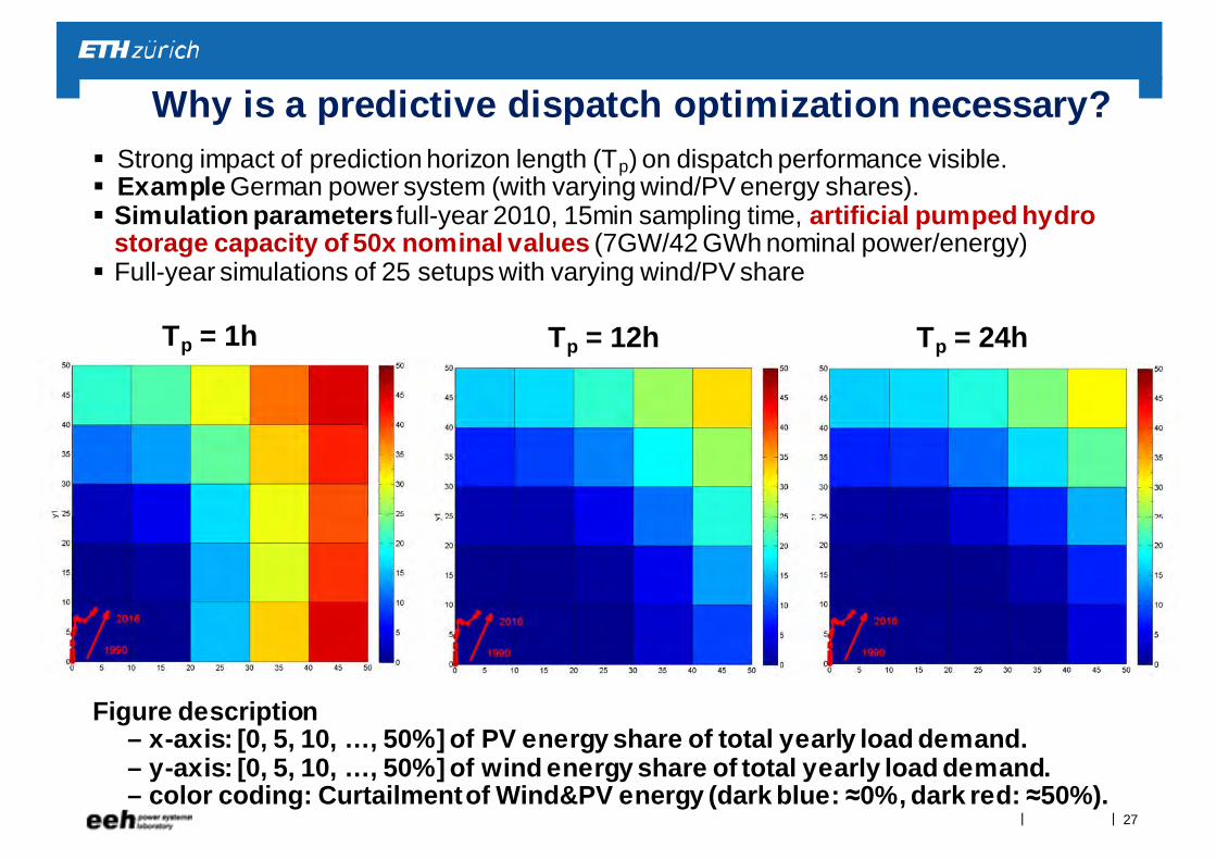
Why is a predictive dispatch optimization necessary? Strong impact of prediction horizon length (Tp) on dispatch performance visible. Example German power system (with varying wind/PV energy shares). Simulation parameters full-year 2010, 15min sampling time, artificial pumped hydro
storage capacity of 50x nominal values (7GW/42 GWh nominal power/energy) Full-year simulations of 25 setups with varying wind/PV share
Figure description– x-axis: [0, 5, 10, …, 50%] of PV energy share of total yearly load demand.– y-axis: [0, 5, 10, …, 50%] of wind energy share of total yearly load demand.– color coding: Curtailmentof Wind&PV energy (dark blue: ≈0%, dark red: ≈50%).
Tp = 1h Tp = 12h Tp = 24h
27
||
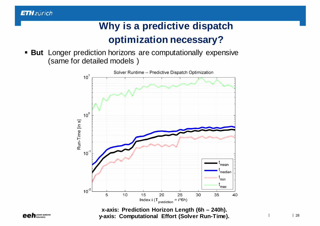
Why is a predictive dispatch optimization necessary?
But Longer prediction horizons are computationally expensive (same for detailed models )
x-axis: Prediction Horizon Length (6h – 240h). y-axis: Computational Effort (Solver Run-Time). 28
||
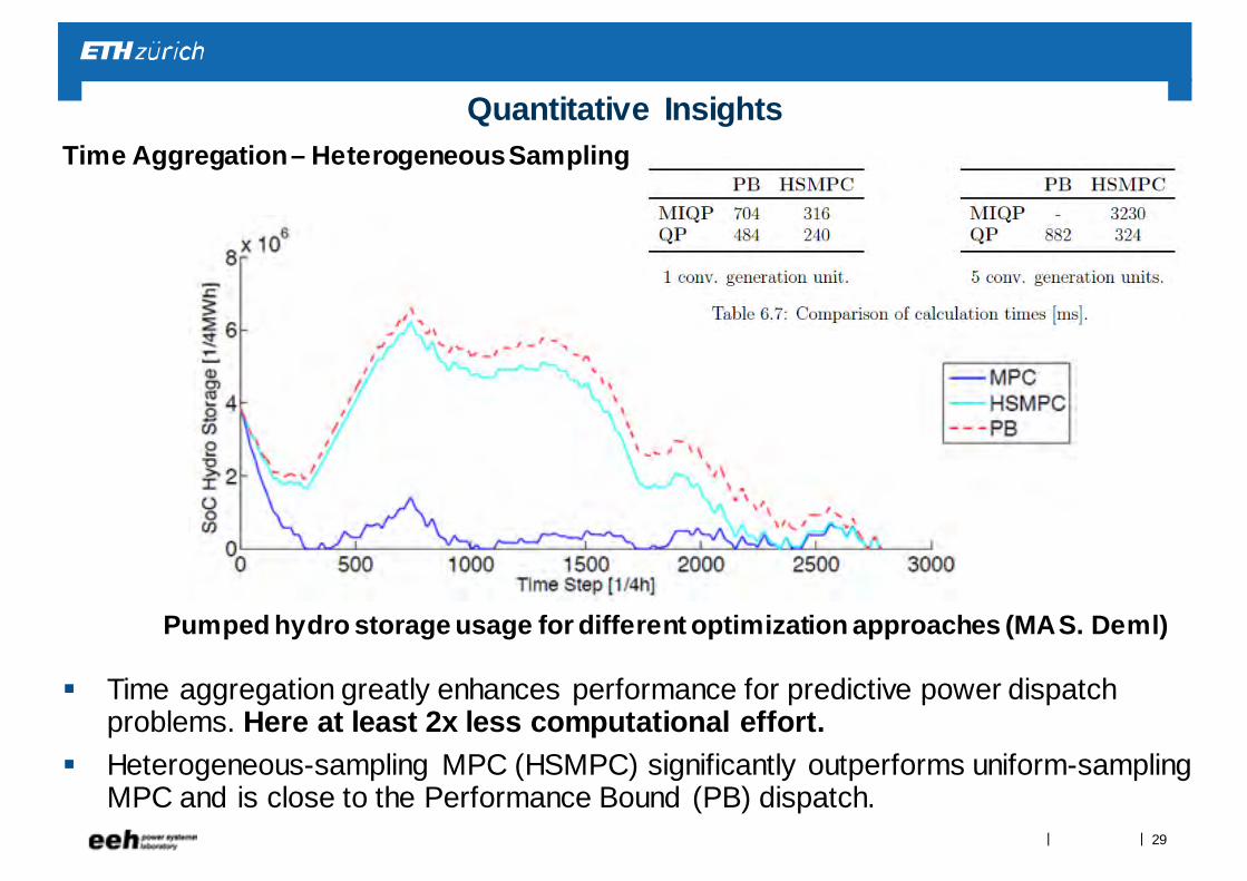
Time Aggregation – Heterogeneous Sampling
Pumped hydro storage usage for different optimization approaches (MA S. Deml)
Time aggregation greatly enhances performance for predictive power dispatch problems. Here at least 2x less computational effort.
Heterogeneous-sampling MPC (HSMPC) significantly outperforms uniform-sampling MPC and is close to the Performance Bound (PB) dispatch.
29
Quantitative Insights
||
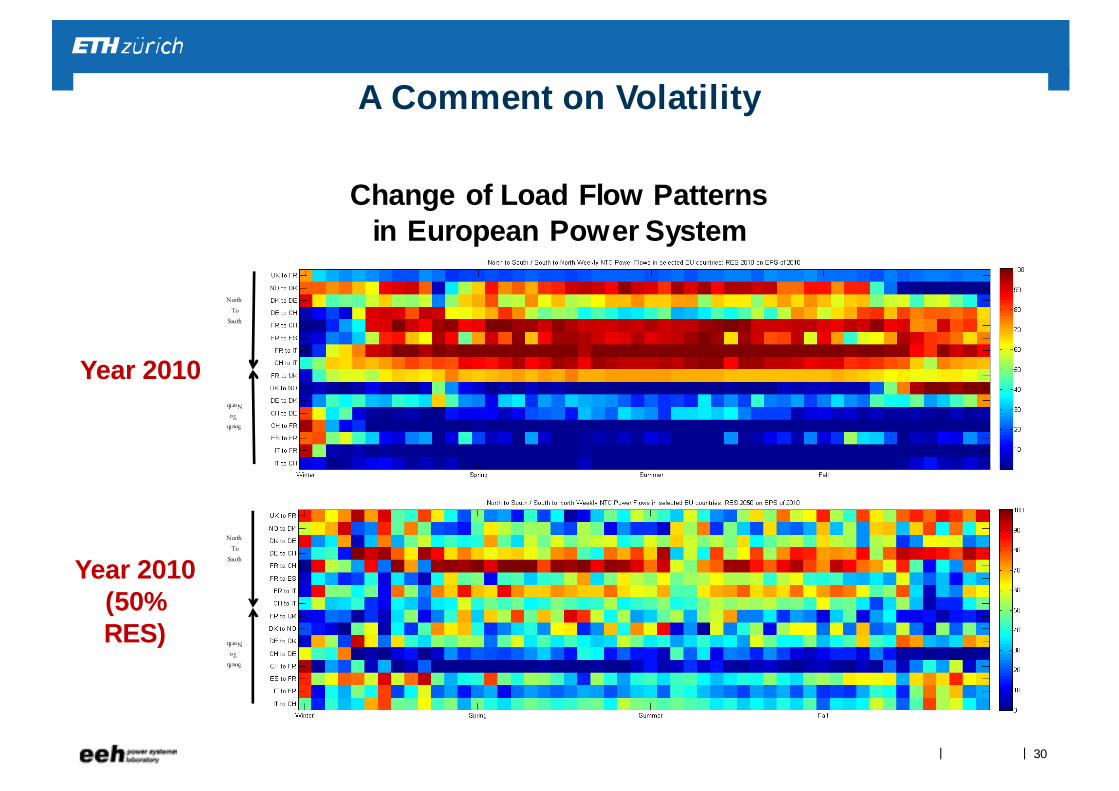
Change of Load Flow Patterns in European Power System
North To
South
South To
North
North To
South
South To
North
Year 2010
Year 2010(50% RES)
30
A Comment on Volatility
||
Cyber-Security in Power Systems
Maria VrakoupouloKostas MargellosPeyman EsfahaniJohn Lygeros
31
||
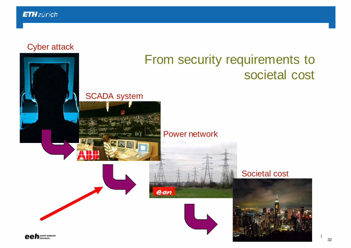
From security requirements to societal cost
Cyber attack
SCADA system
Power network
Societal cost
32
||
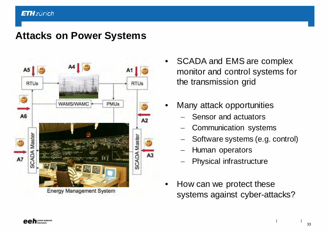
Attacks on Power Systems
• SCADA and EMS are complex monitor and control systems for the transmission grid
• Many attack opportunities Sensor and actuators Communication systems Software systems (e.g. control) Human operators Physical infrastructure
• How can we protect these systems against cyber-attacks?
33
||
Which signals could be manipulated by a cyber-attack?
Generator set points (AGC, etc)
Load tap changers
Status of switches
Configuration changes (macros)
Can we find an attack signal that is able to lead our nominal state in unsafe operation?
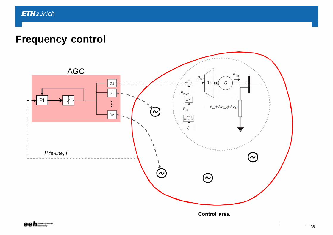
The AGC is one of very few automatically closed loop controllers of the SCADA system. (The only one?)
34
||
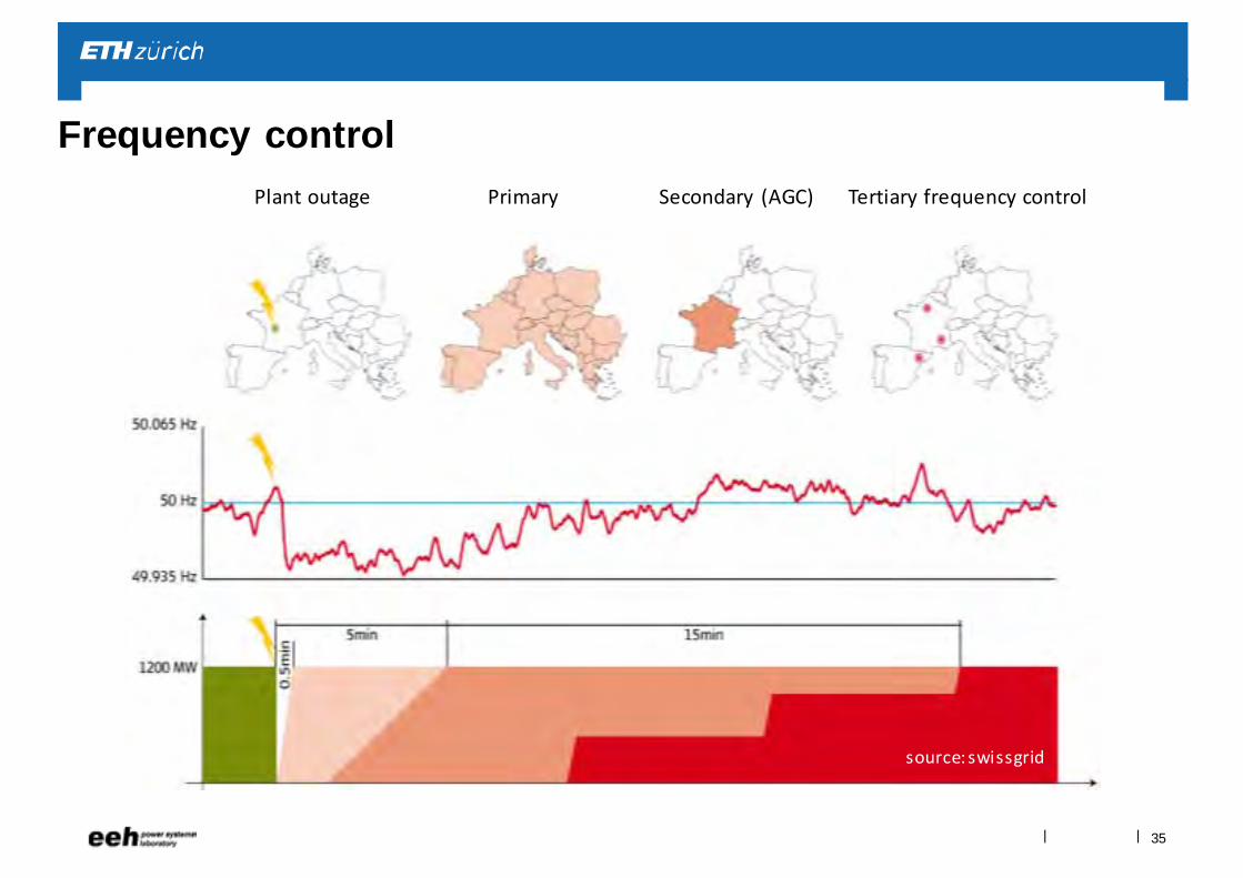
Frequency controlSecondary (AGC)Plant outage Primary Tertiary frequency control
source: swissgrid
35
||
Frequency control
AGC
PI
Ptie-line, f
Control area
d1
d2
dn
36
||
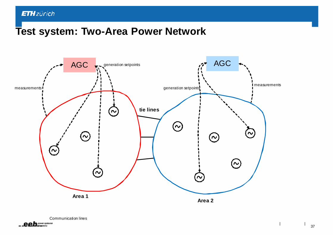
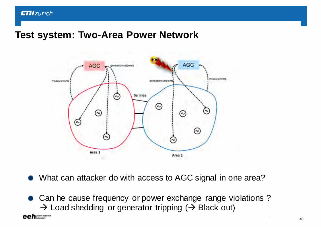
Test system: Two-Area Power Network
tie lines
Area 1Area 2
AGC AGC
measurementsmeasurements
generation setpoints
generation setpoints
Communication lines
37
||
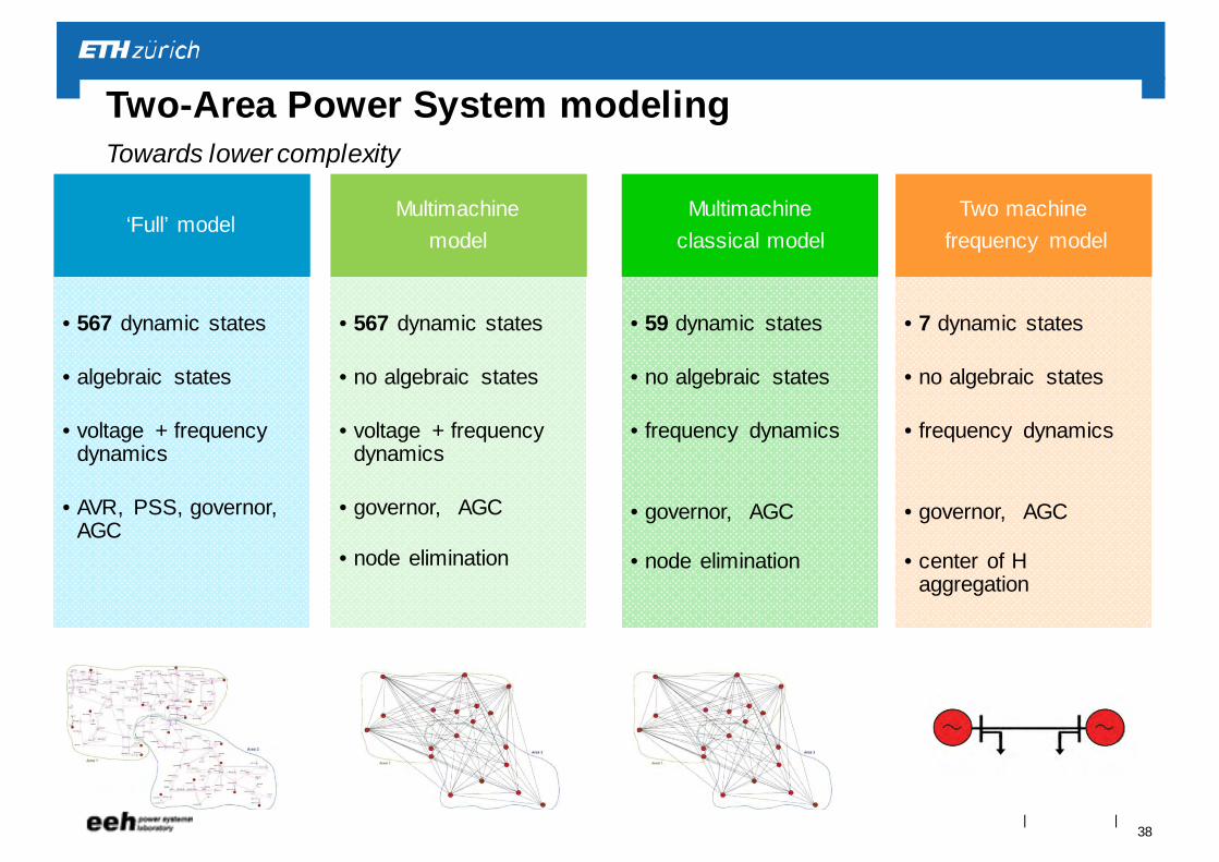
Two-Area Power System modelingTowards lower complexity
‘Full’ model
• 567 dynamic states
• algebraic states
• voltage + frequencydynamics
• AVR, PSS, governor, AGC
Multimachinemodel
• 567 dynamic states
• no algebraic states
• voltage + frequencydynamics
• governor, AGC
• node elimination
Multimachineclassical model
• 59 dynamic states
• no algebraic states
• frequency dynamics
• governor, AGC
• node elimination
Two machine frequency model
• 7 dynamic states
• no algebraic states
• frequency dynamics
• governor, AGC
• center of H aggregation
38
||
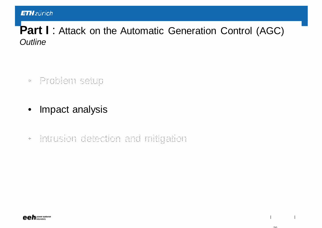
Part I : Attack on the Automatic Generation Control (AGC)Outline
• Problem setup
• Impact analysis
• Intrusion detection and mitigation
39
||
Test system: Two-Area Power Network
What can attacker do with access to AGC signal in one area?
Can he cause frequency or power exchange range violations ? Load shedding or generator tripping ( Black out)
40
||
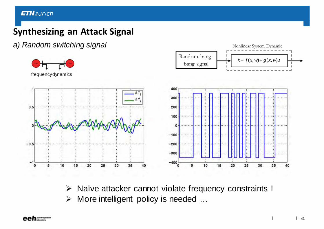
Synthesizing an Attack Signal a) Random switching signal
Naïve attacker cannot violate frequency constraints ! More intelligent policy is needed …
uwxgwxfx ),(),(
Nonlinear System Dynamic
Random bang-bang signal
frequency dynamics
41
||
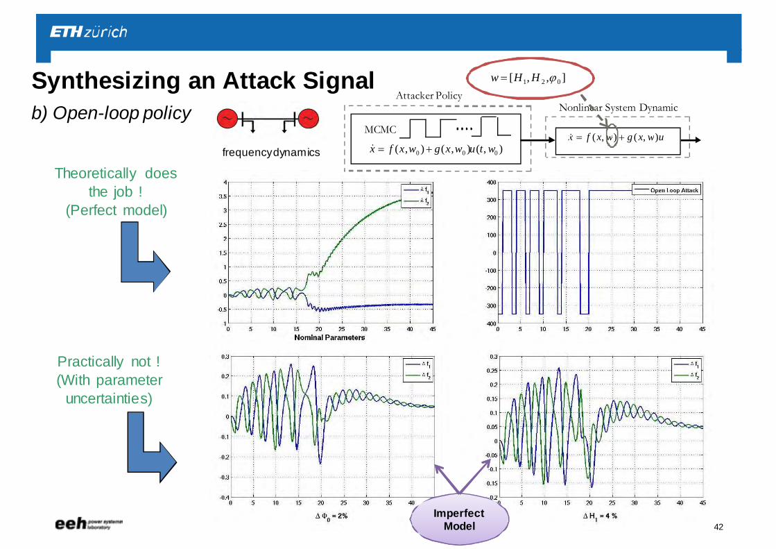
Attacker Policy
uwxgwxfx ),(),(
Nonlinear System Dynamic
MCMC
),(),(),( 000 wtuwxgwxfx
Theoretically does the job !
(Perfect model)
Practically not ! (With parameter
uncertainties)
Imperfect Model
],,[ 021 HHw
frequency dynamics
Synthesizing an Attack Signalb) Open-loop policy
42
||
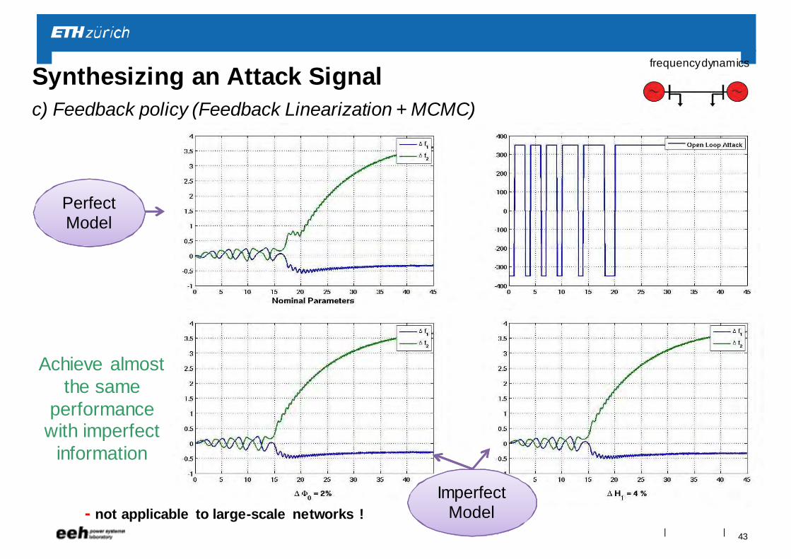
Synthesizing an Attack Signalc) Feedback policy (Feedback Linearization + MCMC)
Achieve almost the same
performance with imperfect
information
Imperfect Model
Perfect Model
frequency dynamics
- not applicable to large-scale networks !43
||
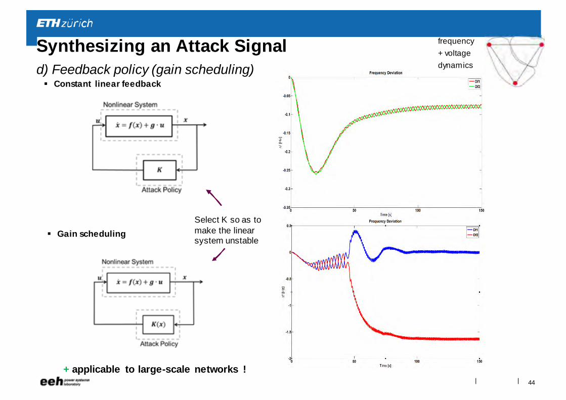
Synthesizing an Attack Signald) Feedback policy (gain scheduling)
Gain scheduling
Constant linear feedback
Select K so as to make the linear system unstable
+ applicable to large-scale networks !
frequency+ voltage dynamics
44
||
Up to now…
• Can attacker cause problems by manipulating AGC?
Yes he can!
With fairly sophisticated feedback controllers
• What can we do about it?
45
||
Part I : Attack on the Automatic Generation Control (AGC)Outline
• Problem setup
• Impact analysis
• Intrusion detection and mitigation
46
||
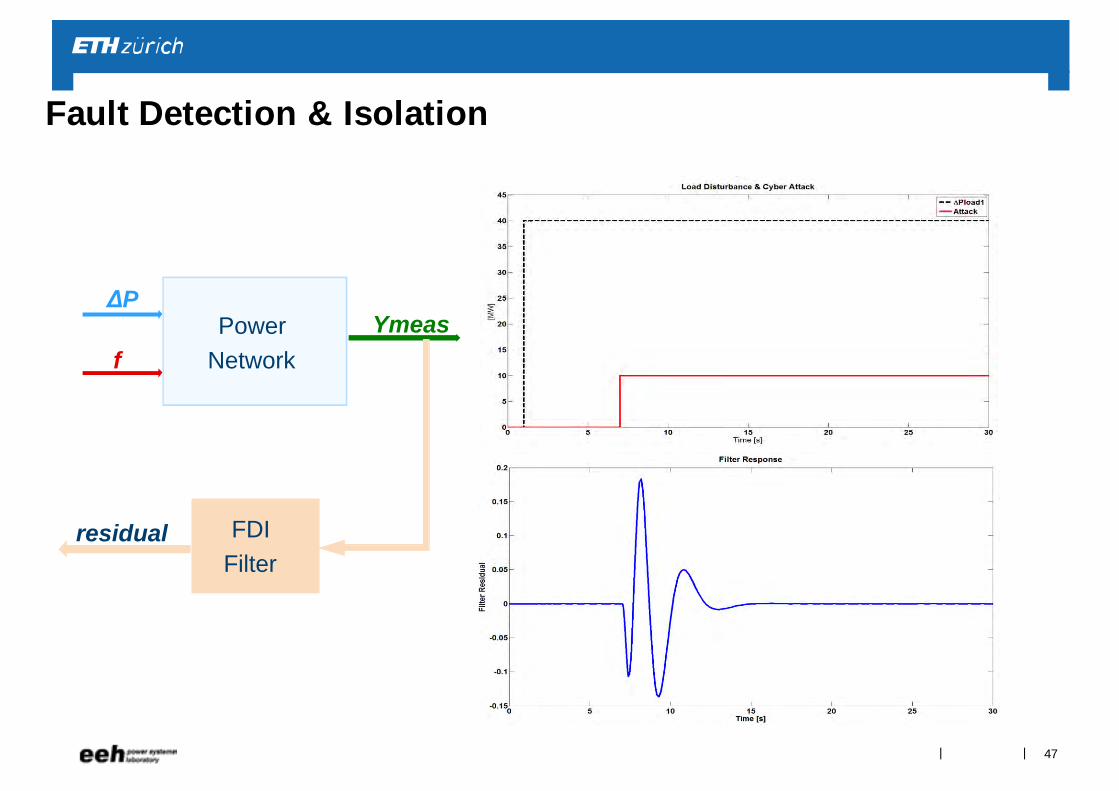
∆P
fYmeasPower
Network
FDIFilter
residual
Fault Detection & Isolation
47
||
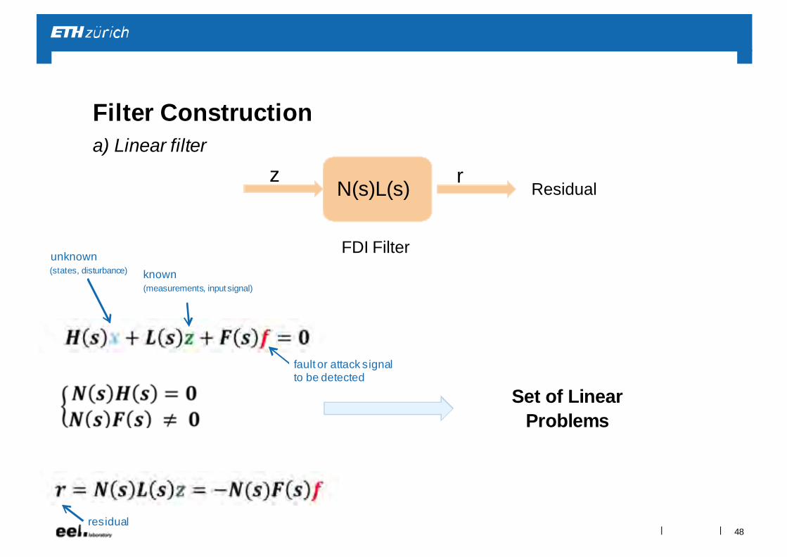
Filter Construction a) Linear filter
Set of Linear Problems
z rN(s)L(s) Residual
FDI Filter
residual
known (measurements, input signal)
unknown(states, disturbance)
fault or attack signalto be detected
48
||
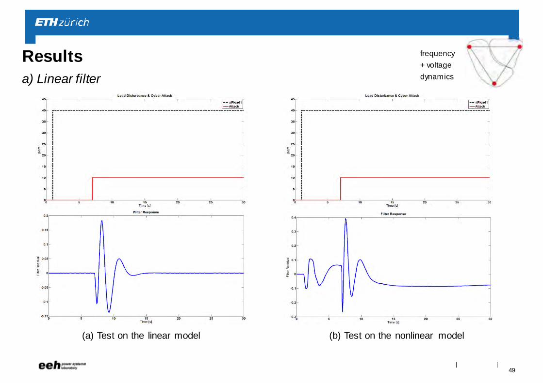
(a) Test on the linear model (b) Test on the nonlinear model
Resultsa) Linear filter
frequency+ voltage dynamics
49
||
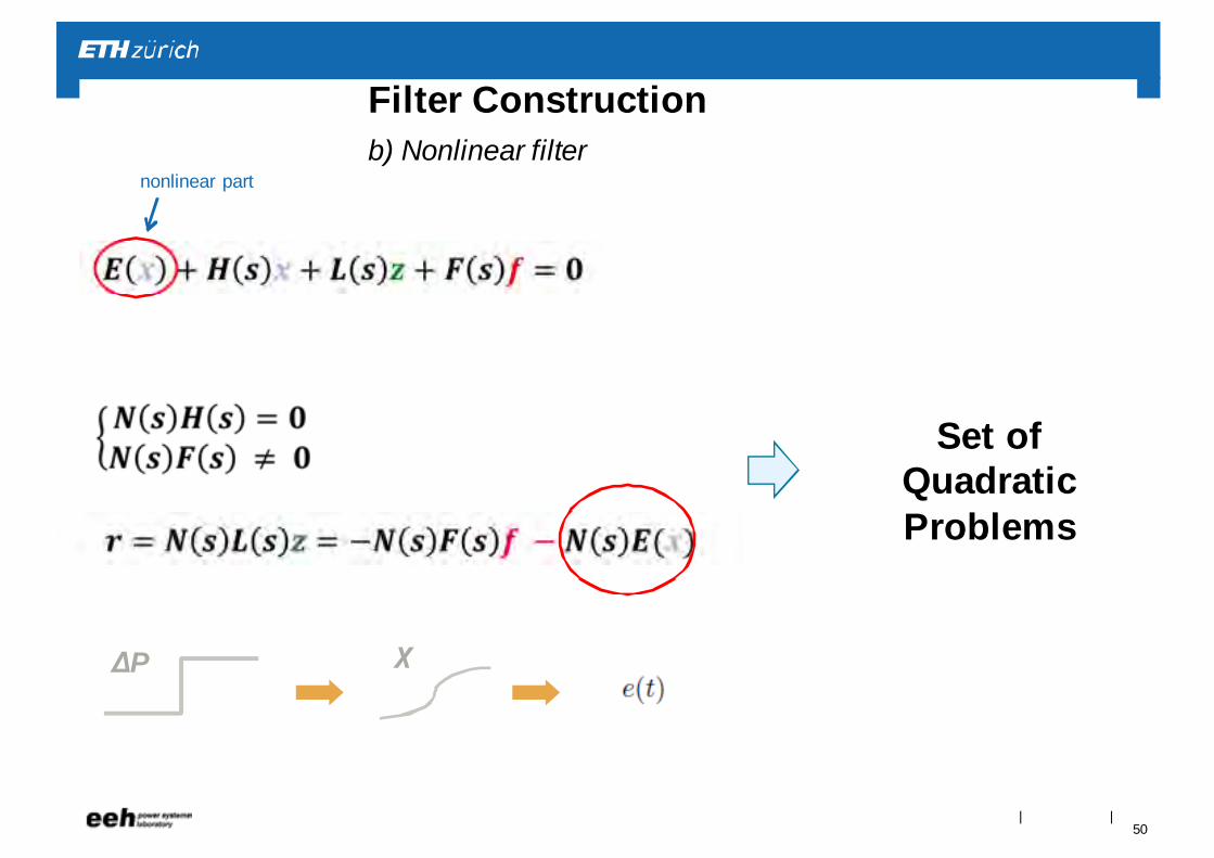
Filter Construction b) Nonlinear filter
∆P χ
Set of QuadraticProblems
nonlinear part
50
||
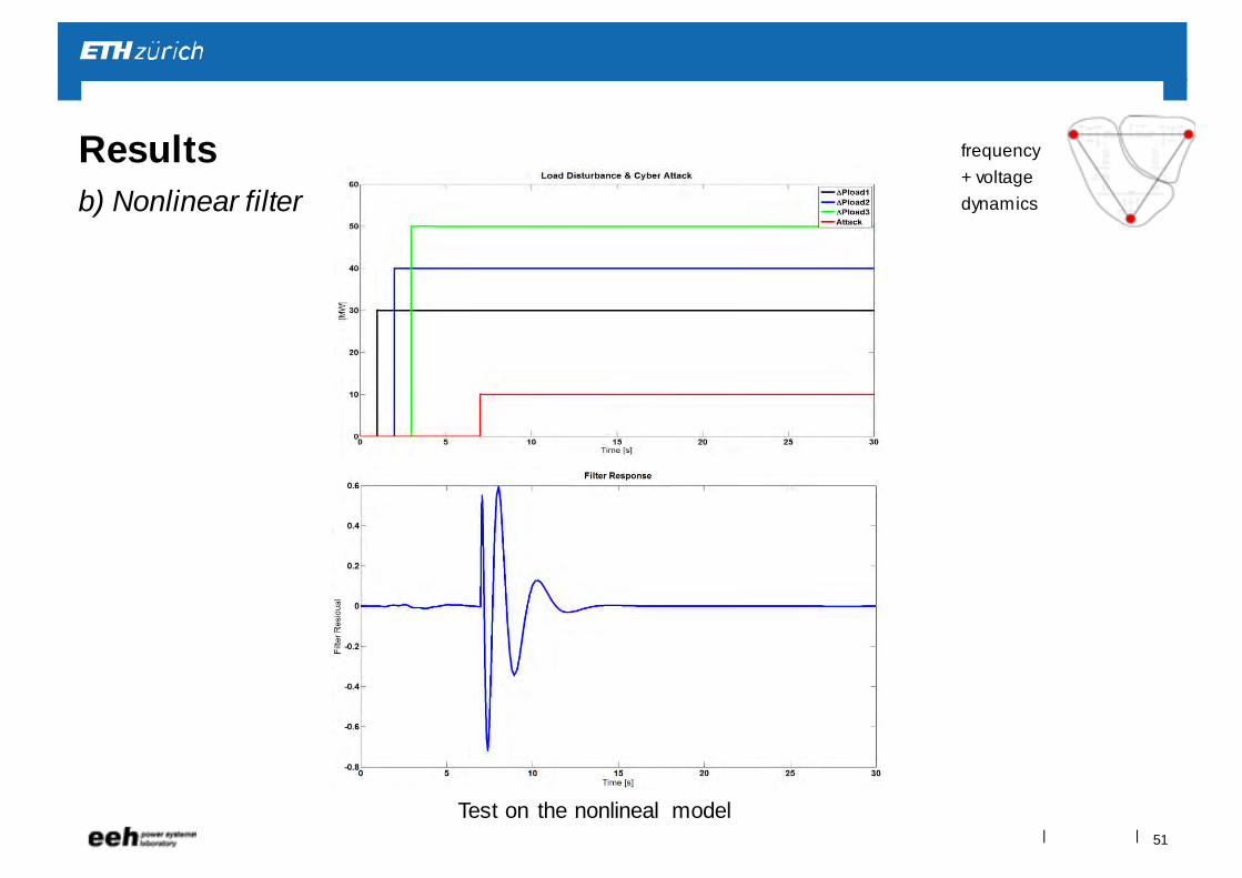
Resultsb) Nonlinear filter
Test on the nonlineal model
frequency+ voltage dynamics
51
||
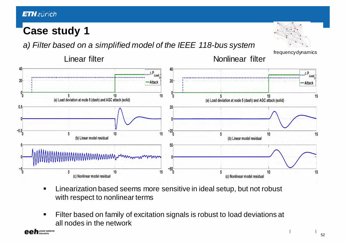
Linearization based seems more sensitive in ideal setup, but not robust with respect to nonlinear terms
Filter based on family of excitation signals is robust to load deviations at all nodes in the network
Linear filter Nonlinear filter
Case study 1a) Filter based on a simplified model of the IEEE 118-bus system
frequency dynamics
52
||
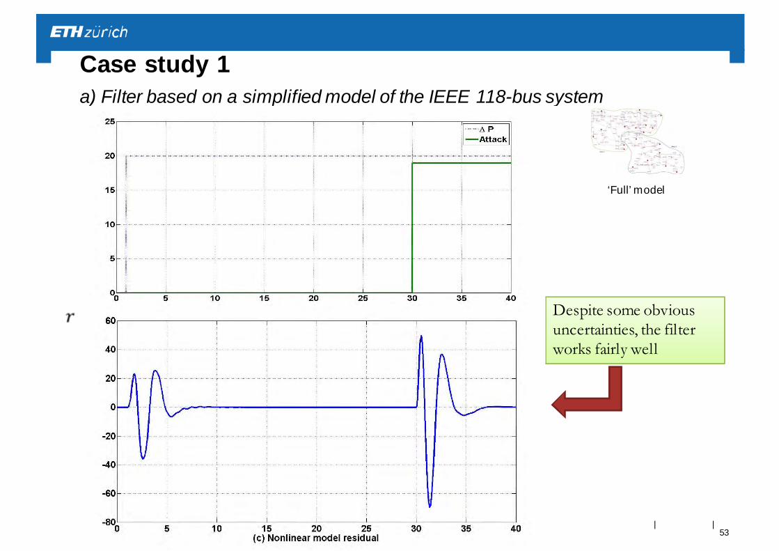
Case study 1a) Filter based on a simplified model of the IEEE 118-bus system
Despite some obvious uncertainties, the filter works fairly well
‘Full’ model
53
||
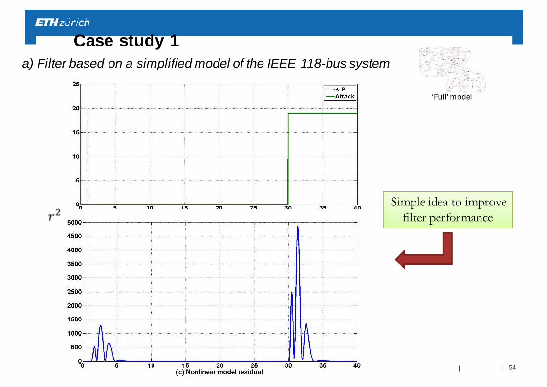
Case study 1a) Filter based on a simplified model of the IEEE 118-bus system
Simple idea to improve filter performance
‘Full’ model
54
||
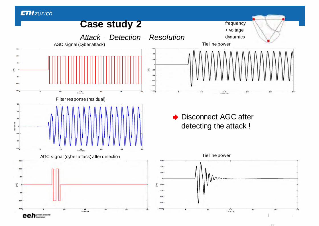
Disconnect AGC after detecting the attack !
Case study 2Attack – Detection – Resolution
frequency+ voltage dynamics
AGC signal (cyber attack) Tie line power
Filter response (residual)
AGC signal (cyber attack) after detection Tie line power
55
||
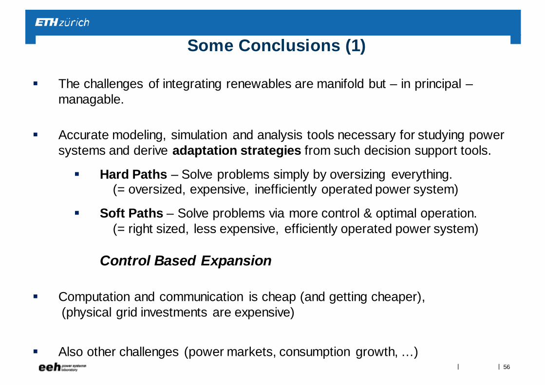
The challenges of integrating renewables are manifold but – in principal –managable.
Accurate modeling, simulation and analysis tools necessary for studying power systems and derive adaptation strategies from such decision support tools.
Hard Paths – Solve problems simply by oversizing everything.(= oversized, expensive, inefficiently operated power system)
Soft Paths – Solve problems via more control & optimal operation.(= right sized, less expensive, efficiently operated power system)
Control Based Expansion
Computation and communication is cheap (and getting cheaper),(physical grid investments are expensive)
Also other challenges (power markets, consumption growth, …)
Some Conclusions (1)
56
||
With the introduction of more (wide-area) control loops, the risks for cyber-attacksincrease
Methods to study cyber-attacks will grow in importance
Means to prevent and identify cyber-attacks will be an essential part of futurepower systems analysis
Some Conclusions (2)
57
|| 58
A general reflection on research
In the middle of the forest there is an unexpected gladethat can only be found by someone who is lost.
Tomas TranströmerNobel Prize Laureate in Literature 2011
||
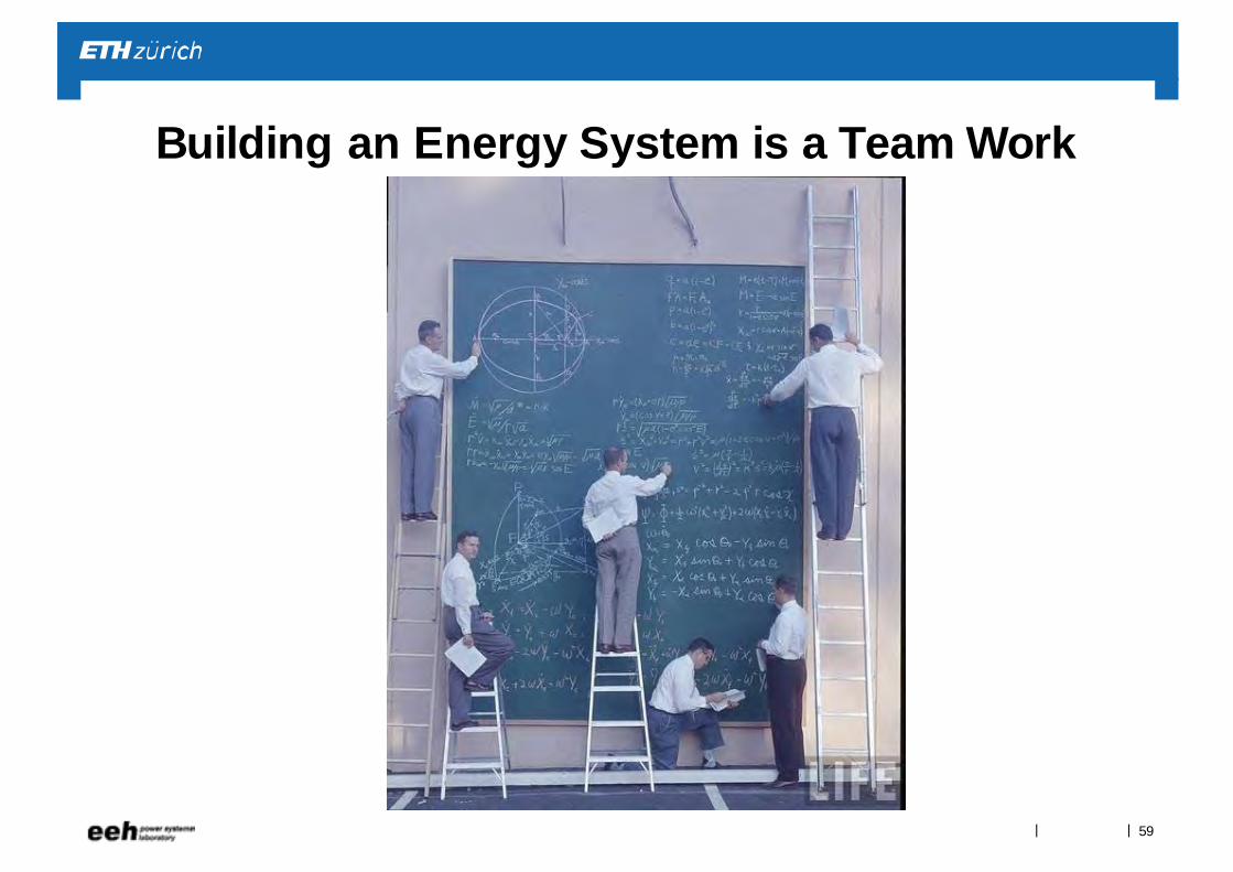
Building an Energy System is a Team Work
59
||
Thank you for your attention
60