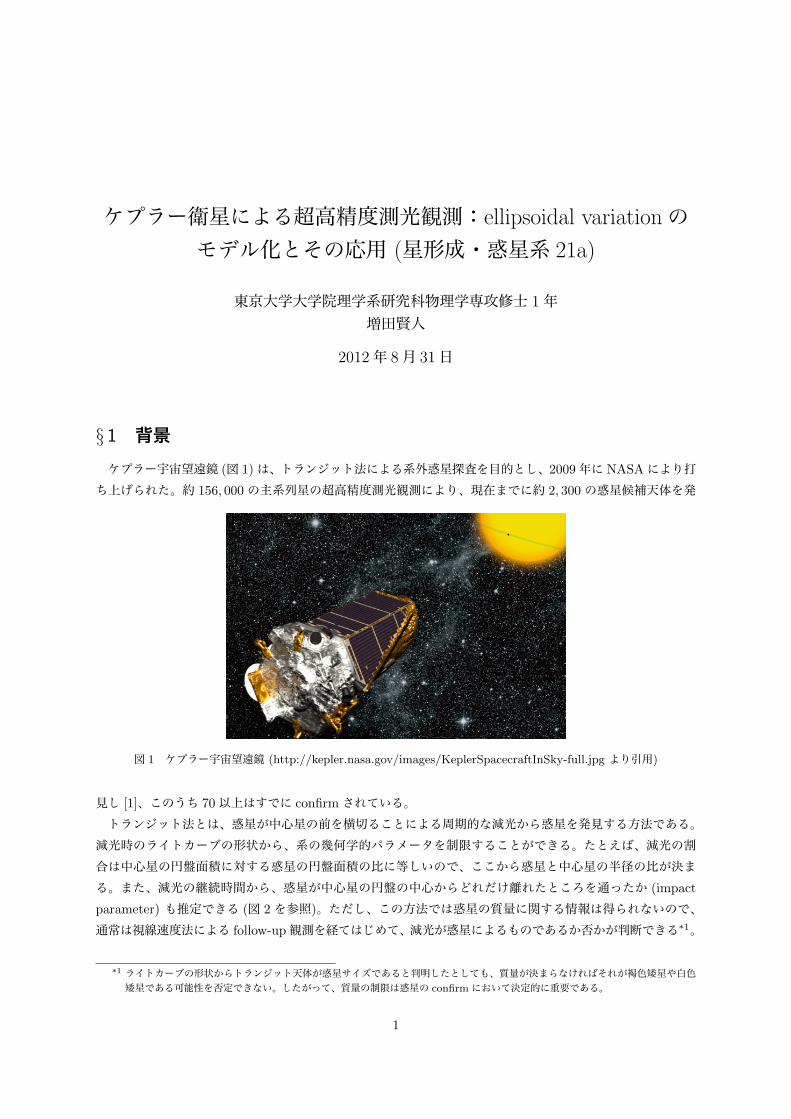
ケプラー衛星による超高精度測光観測：ellipsoidal variationのモデル化とその応用 (星形成・惑星系 21a)

東京大学大学院理学系研究科物理学専攻修士 1年増田賢人

2012年 8月 31日

§ 1 背景ケプラー宇宙望遠鏡 (図 1)は、トランジット法による系外惑星探査を目的とし、2009年に NASAにより打ち上げられた。約 156, 000の主系列星の超高精度測光観測により、現在までに約 2, 300の惑星候補天体を発

図 1 ケプラー宇宙望遠鏡 (http://kepler.nasa.gov/images/KeplerSpacecraftInSky-full.jpg より引用)

見し [1]、このうち 70以上はすでに confirmされている。トランジット法とは、惑星が中心星の前を横切ることによる周期的な減光から惑星を発見する方法である。減光時のライトカーブの形状から、系の幾何学的パラメータを制限することができる。たとえば、減光の割合は中心星の円盤面積に対する惑星の円盤面積の比に等しいので、ここから惑星と中心星の半径の比が決まる。また、減光の継続時間から、惑星が中心星の円盤の中心からどれだけ離れたところを通ったか (impact

parameter) も推定できる (図 2を参照)。ただし、この方法では惑星の質量に関する情報は得られないので、通常は視線速度法による follow-up観測を経てはじめて、減光が惑星によるものであるか否かが判断できる*1。

*1 ライトカーブの形状からトランジット天体が惑星サイズであると判明したとしても、質量が決まらなければそれが褐色矮星や白色矮星である可能性を否定できない。したがって、質量の制限は惑星の confirmにおいて決定的に重要である。

1

図 2 様々な形状のライトカーブ (http://kepler.nasa.gov/files/mws/aas2010-1wbLightCurves.jpgより引用)

ところが、ケプラーがターゲットとしている主系列星の中には、暗すぎて視線速度観測 (スペクトルの測定)

に適さないものも多くある。このような場合に、ライトカーブのみから質量を制限する手段として近年研究されているのが、惑星に由来する微小な周期的変光を利用する方法である ([2][3][4]など)。本講演では、このような質量推定法の概要をまとめるとともに、実際の解析例として EVIL-MC と呼ばれる最新のモデル [5] をKOI-13系に適用して得られた結果を示す。

§ 2 ライトカーブによる質量の推定図 3は、ケプラーが実際に観測した KOI-13のライトカーブである*2。縦軸は、フラックスのトランジットが起きていないときの値からのずれを ppm (1 ppm = 10−6)単位で表したもので、図に示されている 4つの減光 (∼ 5000 ppm) はトランジットによるものである。この図の原点付近を拡大すると、図 4 のように振幅

-5000

-4500

-4000

-3500

-3000

-2500

-2000

-1500

-1000

-500

0

500

140 141 142 143 144 145 146 147 148

ppm

BJD - 2454833.0 [day]

’detrend_Q1_ppm.dat’

図 3 ライトカーブの全体像

-500

-400

-300

-200

-100

0

100

200

300

400

500

140 141 142 143 144 145 146 147 148

’detrend_Q1_ppm.dat’

図 4 拡大図

100 ppm程度の微小な周期変動が見えていることがわかる。これが、先に述べた “惑星由来の微小な周期的変光”である。このような、トランジット (10−3 -10−2 程度)よりさらに 2桁近く小さな信号が検出できていることは、ケプラーの測光精度が非常に高いことの表れである。この変光は 1. ellipsoidal variation 2. relativistic

beaming 3. planetary light の 3つの要因からなっており、これらのうち 1と 2の振幅から惑星質量についての情報を取り出すことができる。そこで、以下ではこれら 3つの要因について概説する。

*2 正確には、quarter 1のデータを 5次多項式でフィットして長期間のトレンドを除いたもの。

2

2.1 ellipsoidal variation

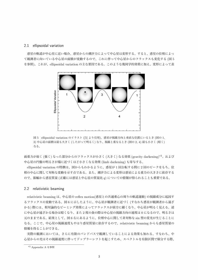
惑星の軌道が中心星に近い場合、惑星からの潮汐力によって中心星は変形する。すると、惑星の位相によって観測者に向いている中心星の面積が変動するので、これに伴って中心星からのフラックスも変化する (図 5

を参照)。これが、ellipsoidal variationの主な要因である。このような幾何学的効果に加え、変形によって表

図 5 ellipsoidal variation のイラスト ([5] より引用)。惑星が視線方向と垂直な位置にいるとき (図の 1,

3)中心星の面積は最も大きく (したがって明るく)なり、視線と重なるとき (図の 2, 4)最も小さく (暗く)

なる。

面重力が弱く (強く)なった部分からのフラックスが小さく (大きく)なる効果 (gravity darkening)*3、および中心星の円盤の明るさが端に近づくほど小さくなる効果 (limb darkening)も寄与する。ellipsoidal variationの特徴は、図からもわかるように、惑星が 1回公転する間に 2回のピークをもち、位相の中心に関して対称な変動を示す点である。また、潮汐力による変形は惑星による重力の大きさに依存するので、振幅から惑星質量 (正確には惑星と中心星の質量比 q)についての情報が得られることも重要である。

2.2 relativistic beaming

relativistic beamingは、中心星の reflex motion(惑星との共通重心の周りの軌道運動)の視線成分に起因するフラックスの変動である。図 6に示したように、中心星が観測者に近づく (すなわち惑星が観測者から遠ざかる)際には、相対論的なビーミング効果によってフラックスが前方に細くなり、中心星が明るく見える。逆に中心星が遠ざかる場合は暗くなり、また 2度の食の際は中心星の視線方向の速度は 0になるので、明るさは元のままである。結果として、図 6右にあるように、位相中心に関して非対称な sin型の変光が生じることになる。ここで、中心星の視線速度もやはり惑星質量に依存するので、relativistic beamingからも惑星質量の情報を得ることができる。実際の観測においては、さらに有限のバンドパスで観測していることによる効果も加わる。すなわち、中心星からの光はその視線速度に伴ってドップラーシフトを起こすため、スペクトルを有限区間で積分する際、

*3 Appendix Aを参照

3

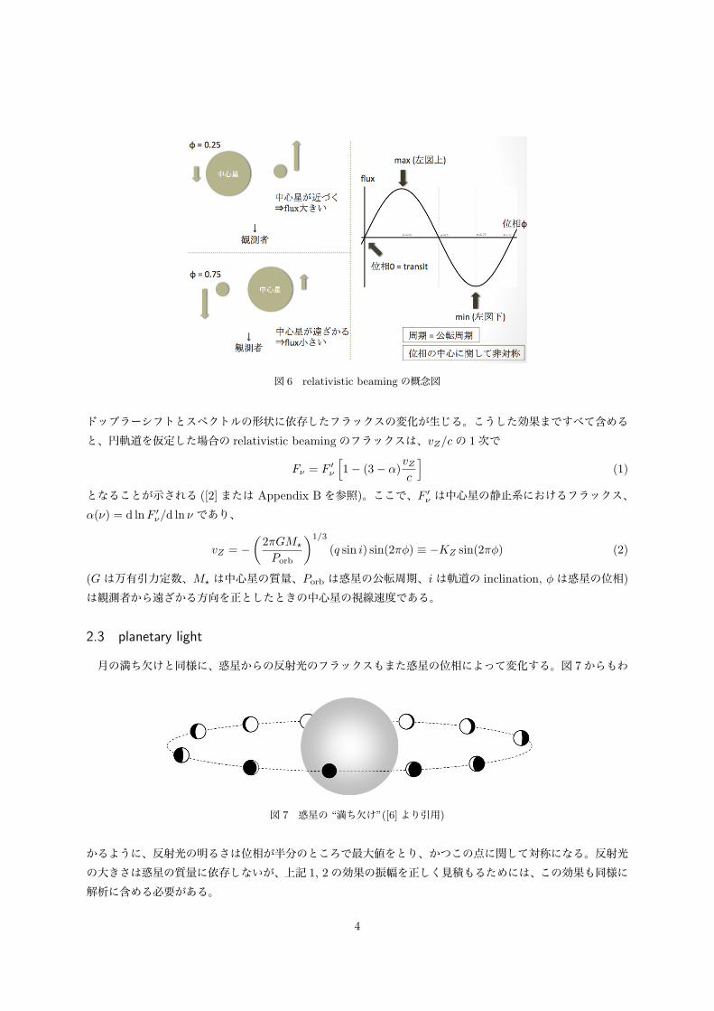
図 6 relativistic beamingの概念図

ドップラーシフトとスペクトルの形状に依存したフラックスの変化が生じる。こうした効果まですべて含めると、円軌道を仮定した場合の relativistic beamingのフラックスは、vZ/cの 1次で

Fν = F ′ν

[1− (3− α)

vZc

](1)

となることが示される ([2]または Appendix Bを参照)。ここで、F ′ν は中心星の静止系におけるフラックス、

α(ν) = d lnF ′ν/d ln ν であり、

vZ = −(2πGM⋆

Porb

)1/3

(q sin i) sin(2πϕ) ≡ −KZ sin(2πϕ) (2)

(Gは万有引力定数、M⋆ は中心星の質量、Porb は惑星の公転周期、iは軌道の inclination, ϕは惑星の位相)

は観測者から遠ざかる方向を正としたときの中心星の視線速度である。

2.3 planetary light

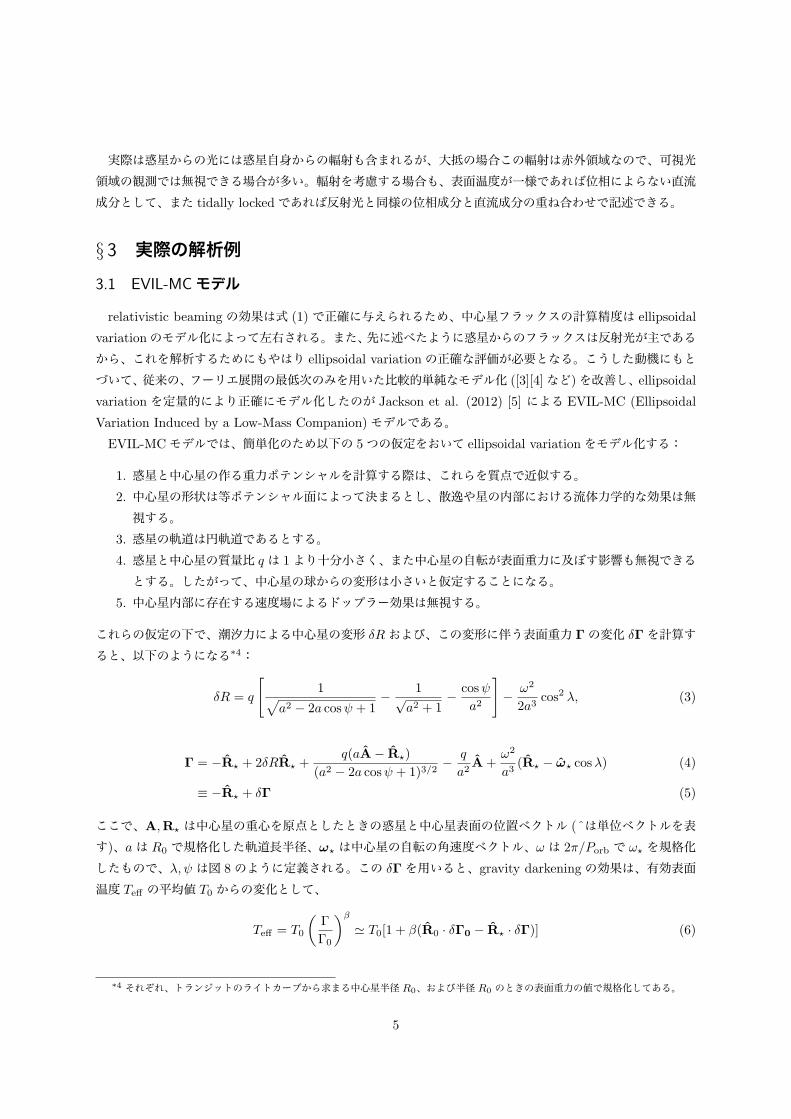
月の満ち欠けと同様に、惑星からの反射光のフラックスもまた惑星の位相によって変化する。図 7からもわ

図 7 惑星の “満ち欠け”([6]より引用)

かるように、反射光の明るさは位相が半分のところで最大値をとり、かつこの点に関して対称になる。反射光の大きさは惑星の質量に依存しないが、上記 1, 2の効果の振幅を正しく見積もるためには、この効果も同様に解析に含める必要がある。

4

実際は惑星からの光には惑星自身からの輻射も含まれるが、大抵の場合この輻射は赤外領域なので、可視光領域の観測では無視できる場合が多い。輻射を考慮する場合も、表面温度が一様であれば位相によらない直流成分として、また tidally lockedであれば反射光と同様の位相成分と直流成分の重ね合わせで記述できる。

§ 3 実際の解析例3.1 EVIL-MCモデル

relativistic beamingの効果は式 (1)で正確に与えられるため、中心星フラックスの計算精度は ellipsoidal

variationのモデル化によって左右される。また、先に述べたように惑星からのフラックスは反射光が主であるから、これを解析するためにもやはり ellipsoidal variationの正確な評価が必要となる。こうした動機にもとづいて、従来の、フーリエ展開の最低次のみを用いた比較的単純なモデル化 ([3][4]など)を改善し、ellipsoidalvariationを定量的により正確にモデル化したのが Jackson et al. (2012) [5] による EVIL-MC (Ellipsoidal

Variation Induced by a Low-Mass Companion)モデルである。EVIL-MCモデルでは、簡単化のため以下の 5つの仮定をおいて ellipsoidal variationをモデル化する：

1. 惑星と中心星の作る重力ポテンシャルを計算する際は、これらを質点で近似する。2. 中心星の形状は等ポテンシャル面によって決まるとし、散逸や星の内部における流体力学的な効果は無視する。

3. 惑星の軌道は円軌道であるとする。4. 惑星と中心星の質量比 q は 1より十分小さく、また中心星の自転が表面重力に及ぼす影響も無視できるとする。したがって、中心星の球からの変形は小さいと仮定することになる。

5. 中心星内部に存在する速度場によるドップラー効果は無視する。

これらの仮定の下で、潮汐力による中心星の変形 δRおよび、この変形に伴う表面重力 Γの変化 δΓを計算すると、以下のようになる*4：

δR = q

[1√

a2 − 2a cosψ + 1− 1√

a2 + 1− cosψ

a2

]− ω2

2a3cos2 λ, (3)

Γ = −R⋆ + 2δRR⋆ +q(aA− R⋆)

(a2 − 2a cosψ + 1)3/2− q

a2A+

ω2

a3(R⋆ − ω⋆ cosλ) (4)

≡ −R⋆ + δΓ (5)

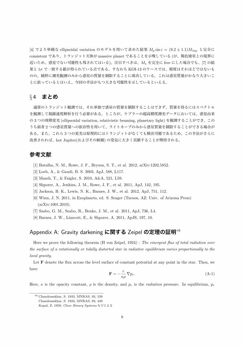
ここで、A,R⋆ は中心星の重心を原点としたときの惑星と中心星表面の位置ベクトル (ˆは単位ベクトルを表す)、aは R0 で規格化した軌道長半径、ω⋆ は中心星の自転の角速度ベクトル、ω は 2π/Porb で ω⋆ を規格化したもので、λ, ψ は図 8のように定義される。この δΓを用いると、gravity darkeningの効果は、有効表面温度 Teff の平均値 T0 からの変化として、

Teff = T0

(Γ

Γ0

)β

≃ T0[1 + β(R0 · δΓ0 − R⋆ · δΓ)] (6)

*4 それぞれ、トランジットのライトカーブから求まる中心星半径 R0、および半径 R0 のときの表面重力の値で規格化してある。

5

図 8 λ, ψ の定義 ([5]より引用)

と表せる。ここで、β は gravity-darkening coefficientと呼ばれる定数である (Appendix A: Zeipelの定理を参照)。また、limb darkening の効果は、法線方向との intensity の比として、foreshortening angle の余弦µ = Γ · Zを用いて

I(µ)

I(1)= 1− γ1(1− µ)− γ2(1− µ)2 (7)

と表せるとする。γ1, γ2 は limb-darkening coefficients と呼ばれる定数である。以上 3 つの効果を合わせると、中心星からのフラックスは、Planck function Bν を用いて

F ′⋆ν(ϕ) =

∫visible surface

Bν(T0)R20 µdΩ×

(1 + 2 δR) ·

[1 + (3− α)

Teff − T0T0

]· I(µ)I(1)

(8)

となる。右辺の brace 内の各項が順に変形、gravity darkening、limb darkening に対応している。これをrelativistic beamingの式 (1)に代入し、ケプラーの response function*5 と畳み込んだものを、観測される中心星のフラックス F⋆ とする。惑星からのフラックス Fp は惑星表面における反射過程の詳細に大きく依存するので、その正確なモデル化は困難である。そこで、先に述べた位相依存性を鑑みて、中心星フラックスとの比をとって単純に

Fp

F⋆= F0 − F1 cos(2πϕ). (9)

とモデル化する。以上のようにして求まる F⋆ と Fp を足し合わせたものが、EVIL-MCモデルにおいて観測される総フラックスとなる。これを用いて実際のライトカーブをフィッティングし、ベストフィットからパラメータ (今回は、上記の式における q, F0, F1(と中心星質量M⋆))を決定する*6。

*5 http://keplergo.arc.nasa.gov/CalibrationResponse.shtml*6 その他のパラメータは観測的に求められた値に固定する。

6

3.2 KOI-13系への適用

今回は、この EVIL-MC モデルを KOI-13 系に適用して解析を行なった*7。フィッティングの結果は図 9

の通りで、2つのピークが ellipsoidal variationによるもの、ピークの高さの差が relativistic beaming(中心について非対称)によるもの、そして位相 0.5の極小値と両端の最小値の差が planetary lightによるものというように、3つの効果によって現実のライトカーブの特徴がよく再現できていることがわかる。フィッティン

図 9 EVIL-MCモデルによるベストフィット。縦軸は平均からの変動 (ppm単位)、横軸は位相。グレーの細かい点は phasefoldした全データ点で、エラーバー付きの点はそれを binningしたもの (位相 0.02刻み)。黒の実線が EVIL-MC によるベストフィットのライトカーブで、色付きの線はそれを各成分に分けたもの。

グは、中心星質量として spectroscopic に求めた値M⋆ = 2.05M⊙([7]) を用いた場合と、中心星質量も free

parameterとした場合の 2通り行ない、ベストフィットから求めたパラメータの値はそれぞれ以下の表 1のようになった。

表 1 ベストフィットのパラメータ

M⋆ = 2.05M⊙ : fix M⋆ : free

q (4.37± 0.05)× 10−3 (4.38± 0.05)× 10−3

F0 (95± 9) ppm (95± 9) ppm

F1 (64.9± 0.6) ppm (64.9± 0.6) ppm

M⋆ - (1.9± 0.3)M⊙

M⋆ を fix した場合の q の値を用いると、惑星質量 Mp は Mp = (9.4 ± 0.9)MJup と求まる*8。これは、

*7 この系の (q, F0, F1 以外の)パラメータは、[7][8] などによって詳しく調べられており、EVIL-MCを適用するのに十分な情報が得られている。

*8 [7]ではM⋆ の誤差が与えられていないので、ここでは [4]にならって 10%とした。

7

[4] でより単純な ellipsoidal variation のモデルを用いて求めた結果 Mp sin i = (9.2 ± 1.1)MJup と完全にconsistentであり、トランジット天体がmassive planetであることを示唆している (が、褐色矮星との境界に近いため、惑星でない可能性も残されてはいる)。注目すべきは、M⋆ を完全に freeにした場合でも、[7]の結果と 1σ で一致する値が得られている点である。すなわち KOI-13のケースでは、精度はそれほどではないものの、純粋に測光観測のみから惑星の質量を制限することに成功している。これは惑星質量がかなり大きいことに依っているとはいえ、今回の手法がもつ大きな可能性を示しているといえる。

§ 4 まとめ通常のトランジット観測では、それ単独で惑星の質量を制限することはできず、質量を得るにはスペクトルを観測して視線速度解析を行う必要がある。ところが、ケプラーの超高精度測光データにおいては、惑星由来の 3つの周期変光 (ellipsoidal variation, relativistic beaming, planetary light)を観測することができ、このうち前者 2つの惑星質量への依存性を用いて、ライトカーブのみから惑星質量を制限することができる場合がある。また、これら 3つの変光は原理的にはトランジットがなくても検出可能であるため、この手法がさらに改善されれば、hot Jupiter(およびその候補)の発見に大きく貢献することが期待される。

参考文献[1] Batalha, N. M., Rowe, J. F., Bryson, S. T., et al. 2012, arXiv:1202.5852.

[2] Loeb, A., & Gaudi, B. S. 2003, ApJ, 588, L117.

[3] Mazeh, T., & Faigler, S. 2010, A&A, 521, L59.

[4] Shporer, A., Jenkins, J. M., Rowe, J. F., et al. 2011, ApJ, 142, 195.

[5] Jackson, B. K., Lewis, N. K., Barnes, J. W., et al. 2012, ApJ, 751, 112.

[6] Winn, J. N. 2011, in Exoplanets, ed. S. Seager (Tucson, AZ: Univ. of Arizona Press)

(arXiv:1001.2010).

[7] Szabo, G. M., Szabo, R., Benko, J. M., et al. 2011, ApJ, 736, L4.

[8] Barnes, J. W., Linscott, E., & Shporer, A. 2011, ApJS, 197, 10.

Appendix A: Gravity darkeningに関する Zeipelの定理の証明*9

Here we prove the following theorem (H von Zeipel, 1924) : The emergent flux of total radiation over

the surface of a rotationally or tidally distorted star in radiative equilibrium varies proportionally to the

local gravity.

Let F denote the flux across the level surface of constant potential at any point in the star. Then, we

haveF = − c

κρ∇pr. (A-1)

Here, κ is the opacity constant, ρ is the density, and pr is the radiation pressure. In equilibrium, pr

*9 Chandrasekhar, S. 1933, MNRAS, 93, 539

Chandrasekhar, S. 1933, MNRAS, 93, 449

Kopal, Z. 1959, Close Binary Systemsなどによる

8

satisfies

∇ ·(

1

κρ∇pr

)= −4πϵρ

c, (A-2)

where 4πϵ stands for the rate of energy liberation (the equation of radiative equilibrium).

On the other hand, the equation of mechanical equilibrium can be written as

∇P = −ρ∇Ψ, (A-3)

where P is the total pressure (gas and radiation) and Ψ is given by

Ψ = V + V ′ + Vrot (A-4)

In eq.(A-4), V denotes the gravitational potential arising from the mass distribution of the star; V ′ is the

tide-generating potential arising from the secondary; Vrot is the centrifugal potential of any particular

layer, rotating around an axis that it perpendicular to the orbital plane with the angular velocity ω. As

so defined, these potentials satisfy the following Poisson’s equations:

∇2V = 4πGρ, (A-5)

∇2V ′ = 0, (A-6)

∇2V = −2ω2, (A-7)

From these equations, it can be shown that surfaces of constant Ψ (level surfaces) are also surfaces of

constant P and ρ, and hence T, pr, κ must be some functions of Ψ. Using eqs.(A-5)-(A-7), eq.(A-3) yields

∇ ·(1

ρ∇P

)= −4πGρ+ 2ω2 (A-8)

Since P and pr are constant over a level surface*10, we may consider pr as a function of P and rewrite

eq.(A-2) as

∇ ·(1

κ

dprdP

· 1ρ∇P

)= −4πϵρ

c, (A-9)

which gives*11

d

dP

(1

κ

dprdP

)1

ρ(∇P )2 + 1

κ

dprdP

∇ ·(1

ρ∇P

)= −4πϵρ

c. (A-10)

Substituting eq.(A-8) into eq.(A-10), we find

d

dP

(1

κ

dprdP

)1

ρ(∇P )2 = −4πϵρ

c+

1

κ

dprdP

(4πGρ− 2ω2), (A-11)

whose right-hand side is a constant over a level surface*12. Hence the left-hand side is either constant over

a level surface or is identically zero. If it were a constant over a level surface, so is |∇P |, which requires

that the equipotntial surafaces are parallel. This is impossible for a tidally distorted configuration, and

so we should haved

dP

(1

κ

dprdP

)= 0 (A-12)

*10 as discussed in the previous paragraph*11 ∇ · (ϕ∇ψ) = ∇ϕ · ∇ψ + ϕ∇2ψ*12 This follows from the same discussion as referred in the footnote 5

9

or1

κ

dprdP

= const. ≡ β (A-13)

From this equation, together with eqs.(A-1) and (A-3), the flux F across the level surface is given by

F = − c

κρ

dprdP

∇P = cβ∇Ψ. (A-14)

Since ∇Ψ is identical with the local gravity, the validity of von Zeipel’s theorem is thus demonstrated.

Appendix B: Relativistic beamingの式 (1)の導出B-1. Angular Distribution of Received Power*13

Let us consider a particle moving at (relativistic) velocity v in the x direction in a certain inertial

frame K. We also consider an instantaneous rest frame K ′, in which the particle has zero velocity

instantaneously (= at least for infinitesimally neighboring times). Suppose that, in the instantaneous

rest frame, an amount of power dP ′ is emitted from the particle into the solid angle dΩ′, then the power

recieved by an observer in frame K (per solid angle) is given by

dP

dΩ=

dW

dΩdt=

dW

dW ′dΩ′

dΩ

dt′

dt

dW ′

dΩ′ dt′=

dW

dW ′dΩ′

dΩ

dt′

dt

dP ′

dΩ′ .　 (B-1)

(i) dW/dW ′ (Energy transformation)

Let us consider an amount of energy dW ′ and momentum dp′ is emitted into the solid angle dΩ′ =

d(cos θ′)dϕ′ ≡ dµ′dϕ′ about the direction (θ′, ϕ′), where θ′(or θ) is measured from the x′(or x) axis.

Then, the Lorentz transformation of the four-vector gives the energy dW obeserved in frame K:

dW = γ(dW ′ + vdp′x) = γ(1 + βµ′)dW ′. (B-2)

Here, we used dp′x = (dW ′/c) cos θ′ = βµ′dW ′.

(ii) dΩ/dΩ′ (Aberration of light)

For velocities in frame K and K ′, we have the relation

u∥ =u′∥ + v

1 + vu′∥/c2, u⊥ =

u′⊥γ(1 + vu′∥/c

2), (B-3)

where ∥ denotes the component parallel to v (= x component), and ⊥ perpendicular to it. This gives,

in the case of |u| = c,

cos θ =u∥

c=

cos θ′ + β

1 + β cos θ′or µ =

µ′ + β

1 + βµ′ . (B-4)

Differentiating this equation and using dϕ = dϕ′, we have the transformation of the solid angle, given by

dΩ = dµdϕ =dµ′

γ2(1 + βµ′)2dϕ =

dΩ′

γ2(1 + βµ′)2. (B-5)

*13 Rybicki and Lightman, “Radiative Processes in Astrophysics”, pp. 140-142による

10

(iii) dt/dt′

Suppose that the light is emitted in K ′ frame during the time interval of dt′ and observed in the

direction θ with respect to the velocity of the particle in frame K. Then, that interval is given by

dt = γ dt′ in frame K, for the particle is at rest in frame K ′. Since the particle in frame K travels vµdt

along the observer’s line of sight during this interval, the time interval dtA during which an observer in

K receives the radiation is

dtA = dt(1− βµ) = γ(1− βµ)dt′ =dt′

γ(1 + βµ′). (B-6)

In the last equation, we used the relation

1− βµ =1

γ2(1 + βµ′)(B-7)

obtained from eq.(B-4). Here, we use this dtA as the value of dt in dt/dt′.

We also have the relation of frequencies in these two frames (Doppler effect), taking dt′ as a period of

emission in frame K ′. The result isν = γ(1 + βµ′)ν′. (B-8)

♣ Remark

If we choose, in the step (iii), dt = γ dt′, then this is the time interval of emission in frame K. With

this choice, we obtain dP/dΩ as the emitted power per solid angle in frame K.

From (i)-(iii), we get the transformation

dP

dΩ= γ4(1 + βµ′)4

dP ′

dΩ′ =1

γ4(1− βµ)4dP ′

dΩ′ . (B-9)

Here, we again used eq.(B-7). Note that the inverse fransformation is obtained by interchanging primed

and unprimed quantities, along with changing the sign of β (emitted power does not have such symmetry

property).

B-2. “Beaming” Formula*14

Hereafter, we will use F for dP/dΩ and vr ≡ βµ for the radial velocity of the particle in frame K. For

vr ≪ c, eqs. (B-9) and (B-8) yield

F = F ′(1 + 4

vrc

)(B-10)

ν = ν′(1 +

vrc

). (B-11)

Assuming that F ′ν′ ∝ ν′α, from these eqs.(B-10) and (B-11) we have

Fν = F ′ν

[1 + (3− α)

vrc

]. (B-12)

*14 [2]による

11

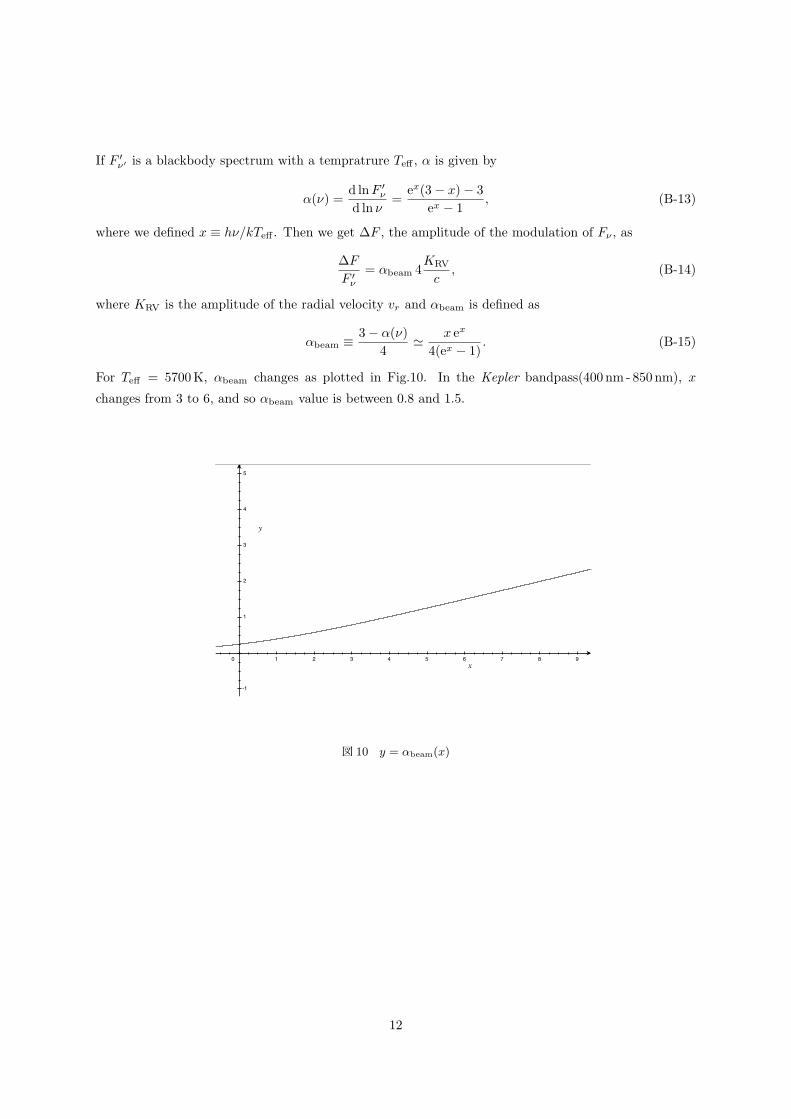
If F ′ν′ is a blackbody spectrum with a tempratrure Teff , α is given by

α(ν) =d lnF ′

ν

d ln ν=

ex(3− x)− 3

ex − 1, (B-13)

where we defined x ≡ hν/kTeff . Then we get ∆F , the amplitude of the modulation of Fν , as

∆F

F ′ν

= αbeam 4KRV

c, (B-14)

where KRV is the amplitude of the radial velocity vr and αbeam is defined as

αbeam ≡ 3− α(ν)

4≃ x ex

4(ex − 1). (B-15)

For Teff = 5700K, αbeam changes as plotted in Fig.10. In the Kepler bandpass(400 nm - 850 nm), x

changes from 3 to 6, and so αbeam value is between 0.8 and 1.5.

0 1 2 3 4 5 6 7 8 9

-1

1

2

3

4

5

図 10 y = αbeam(x)

12