Embed Size (px)
Citation preview

テンソル分解による関係データ解析
林 浩平
東京大学 学振特別研究員 (PD)
2012年 11月 14日ERATO湊離散構造処理系プロジェクト セミナー
1 / 27
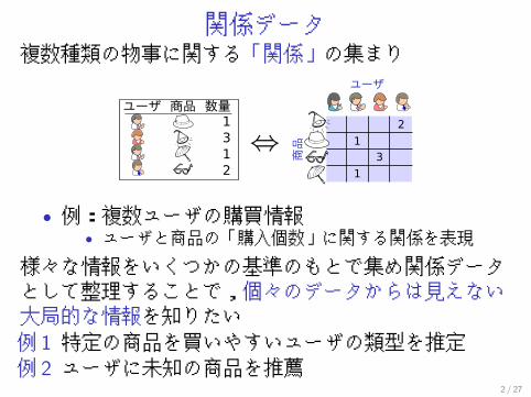
関係データ複数種類の物事に関する「関係」の集まり
• 例:複数ユーザの購買情報• ユーザと商品の「購入個数」に関する関係を表現
様々な情報をいくつかの基準のもとで集め関係データとして整理することで,個々のデータからは見えない大局的な情報を知りたい例 1 特定の商品を買いやすいユーザの類型を推定例 2 ユーザに未知の商品を推薦
2 / 27
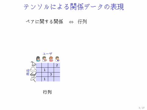
テンソルによる関係データの表現
ペアに関する関係 ⇔ 行列
3 / 27
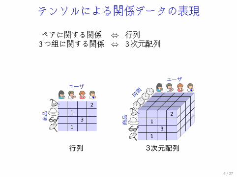
テンソルによる関係データの表現
ペアに関する関係 ⇔ 行列3つ組に関する関係 ⇔ 3次元配列
4 / 27
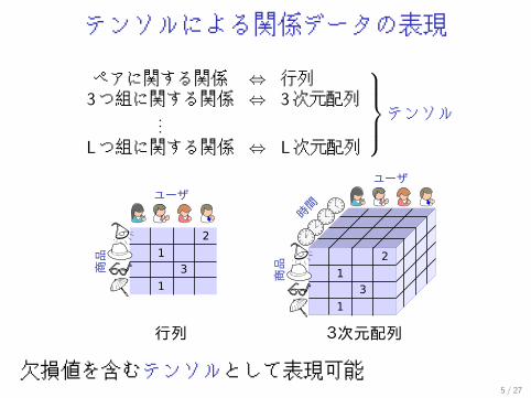
テンソルによる関係データの表現
ペアに関する関係 ⇔ 行列3つ組に関する関係 ⇔ 3次元配列
...Lつ組に関する関係 ⇔ L次元配列
⎫⎪⎪⎬⎪⎪⎭テンソル
欠損値を含むテンソルとして表現可能5 / 27
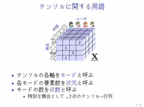
テンソルに関する用語
• テンソルの各軸をモードと呼ぶ• 各モードの要素数を次元と呼ぶ• モードの数を次数と呼ぶ
• 特別な場合として,2次のテンソル=行列
6 / 27
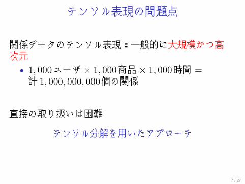
テンソル表現の問題点
関係データのテンソル表現:一般的に大規模かつ高次元
• 1, 000ユーザ× 1, 000商品× 1, 000時間 =計 1, 000, 000, 000個の関係
直接の取り扱いは困難
テンソル分解を用いたアプローチ
7 / 27
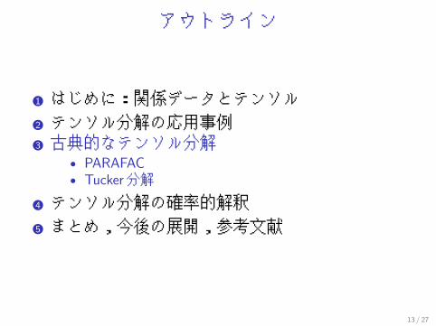
アウトライン
1 はじめに:関係データとテンソル2 テンソル分解の応用事例3 古典的なテンソル分解4 テンソル分解の確率的解釈5 まとめ,今後の展開,参考文献
8 / 27
アウトライン
1 はじめに:関係データとテンソル2 テンソル分解の応用事例3 古典的なテンソル分解4 テンソル分解の確率的解釈5 まとめ,今後の展開,参考文献
9 / 27
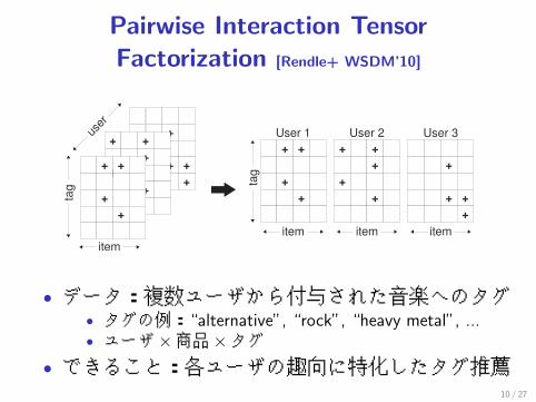
Pairwise Interaction TensorFactorization [Rendle+ WSDM’10]
+
+ ++
+ ++
1+
+ +
++
tag
item
user
+ +
++
+ ++
++
+
+ ++
User 1 User 2 User 3
item item item
tag
• データ:複数ユーザから付与された音楽へのタグ• タグの例:“alternative”, “rock”, “heavy metal”, ...• ユーザ×商品×タグ
• できること:各ユーザの趣向に特化したタグ推薦10 / 27
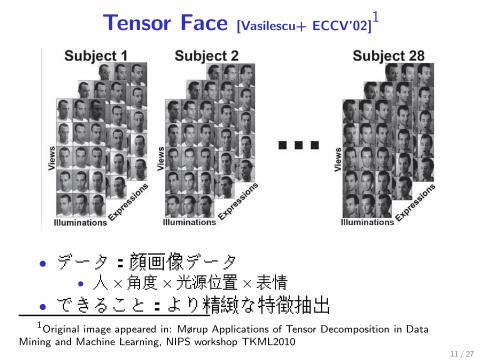
Tensor Face [Vasilescu+ ECCV’02]1
• データ:顔画像データ• 人×角度×光源位置×表情
• できること:より精緻な特徴抽出1Original image appeared in: Mørup Applications of Tensor Decomposition in Data
Mining and Machine Learning, NIPS workshop TKML201011 / 27
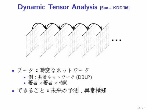
Dynamic Tensor Analysis [Sun+ KDD’06]
• データ:時変なネットワーク• 例:共著ネットワーク (DBLP)• 著者×著者×時間
• できること:未来の予測,異常検知
12 / 27
アウトライン
1 はじめに:関係データとテンソル2 テンソル分解の応用事例3 古典的なテンソル分解
• PARAFAC• Tucker分解
4 テンソル分解の確率的解釈5 まとめ,今後の展開,参考文献
13 / 27
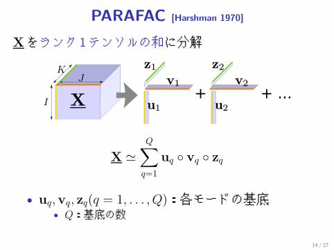
PARAFAC [Harshman 1970]
Xをランク 1テンソルの和に分解
X �Q∑
q=1
uq ◦ vq ◦ zq
• uq,vq, zq(q = 1, . . . , Q):各モードの基底• Q:基底の数
14 / 27
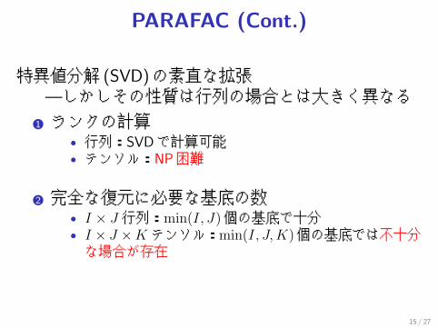
PARAFAC (Cont.)
特異値分解 (SVD)の素直な拡張—しかしその性質は行列の場合とは大きく異なる
1 ランクの計算• 行列:SVDで計算可能• テンソル:NP困難
2 完全な復元に必要な基底の数• I × J 行列:min(I, J)個の基底で十分• I × J ×Kテンソル:min(I, J, K)個の基底では不十分な場合が存在
15 / 27
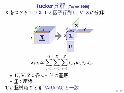
Tucker分解 [Tucker 1966]
XをコアテンソルTと因子行列U,V,Zに分解
xijk �Q∑
q=1
R∑r=1
S∑s=1
tqrsuiqvjrzks
• U,V,Z:各モードの基底• T:座標
Tが超対角のときPARAFACと一致16 / 27
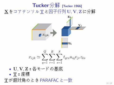
Tucker分解 [Tucker 1966]
XをコアテンソルTと因子行列U,V,Zに分解
xijk �Q∑
q=1
R∑r=1
S∑s=1
tqrsuiqvjrzks
• U,V,Z:各モードの基底• T:座標
Tが超対角のときPARAFACと一致17 / 27
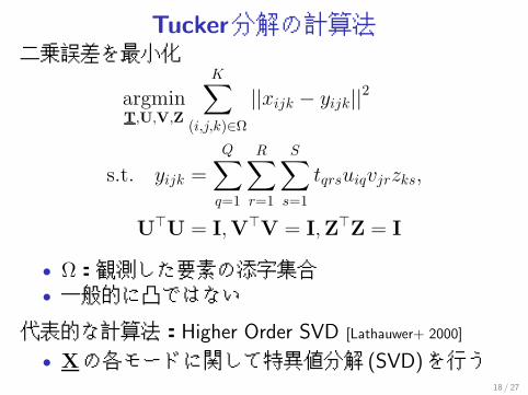
Tucker分解の計算法二乗誤差を最小化
argminT,U,V,Z
K∑(i,j,k)∈Ω
||xijk − yijk||2
s.t. yijk =
Q∑q=1
R∑r=1
S∑s=1
tqrsuiqvjrzks,
U�U = I,V�V = I,Z�Z = I
• Ω:観測した要素の添字集合• 一般的に凸ではない
代表的な計算法:Higher Order SVD [Lathauwer+ 2000]
• Xの各モードに関して特異値分解 (SVD)を行う18 / 27
アウトライン
1 はじめに:関係データとテンソル2 テンソル分解の応用事例3 古典的なテンソル分解4 テンソル分解の確率的解釈5 まとめ,今後の展開,参考文献
19 / 27
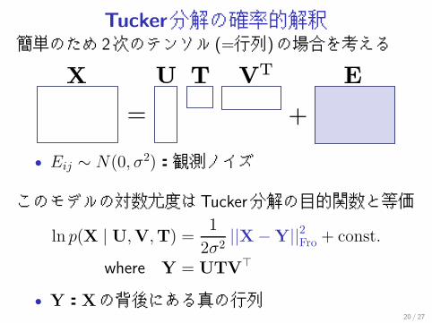
Tucker分解の確率的解釈簡単のため 2次のテンソル (=行列)の場合を考える
• Eij ∼ N(0, σ2):観測ノイズ
このモデルの対数尤度はTucker分解の目的関数と等価
ln p(X | U,V,T) =1
2σ2 ||X −Y||2Fro + const.
where Y = UTV�
• Y:Xの背後にある真の行列20 / 27
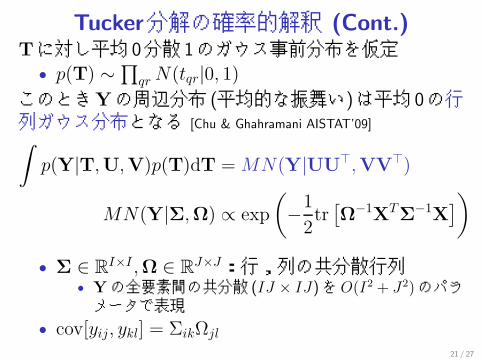
Tucker分解の確率的解釈 (Cont.)Tに対し平均 0分散 1のガウス事前分布を仮定
• p(T) ∼ ∏qr N(tqr|0, 1)
このときYの周辺分布 (平均的な振舞い)は平均 0の行列ガウス分布となる [Chu & Ghahramani AISTAT’09]∫
p(Y|T,U,V)p(T)dT = MN(Y|UU�,VV�)
MN(Y|Σ,Ω) ∝ exp
(−1
2tr
[Ω−1XTΣ−1X
])
• Σ ∈ RI×I ,Ω ∈ R
J×J:行,列の共分散行列• Yの全要素間の共分散 (IJ × IJ)をO(I2 + J2)のパラメータで表現
• cov[yij, ykl] = ΣikΩjl
21 / 27
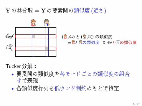
Yの共分散 = Yの要素間の類似度 (近さ)
Tucker分解:• 要素間の類似度を各モードごとの類似度の組合せで表現
• 各類似度行列を低ランク制約のもとで推定
22 / 27
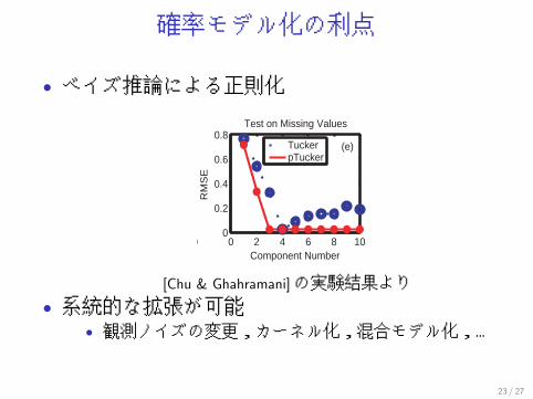
確率モデル化の利点
• ベイズ推論による正則化
0 0 2 4 6 8 100
0.2
0.4
0.6
0.8
Component Number
RM
SE
Test on Missing Values
TuckerpTucker
(e)
[Chu & Ghahramani]の実験結果より• 系統的な拡張が可能
• 観測ノイズの変更,カーネル化,混合モデル化,…
23 / 27
アウトライン
1 はじめに:関係データとテンソル2 テンソル分解の応用事例3 古典的なテンソル分解4 テンソル分解の確率的解釈5 まとめ,今後の展開,参考文献
24 / 27
まとめ
• 関係データ=複数の物事の組に関するデータ• 関係データはテンソルとして表現可能• テンソルの圧縮表現としてのPARAFAC,Tucker分解
• Tucker分解の確率モデル化
25 / 27
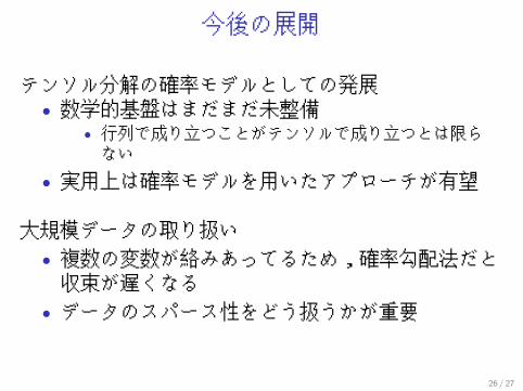
今後の展開
テンソル分解の確率モデルとしての発展• 数学的基盤はまだまだ未整備
• 行列で成り立つことがテンソルで成り立つとは限らない
• 実用上は確率モデルを用いたアプローチが有望
大規模データの取り扱い• 複数の変数が絡みあってるため,確率勾配法だと収束が遅くなる
• データのスパース性をどう扱うかが重要
26 / 27
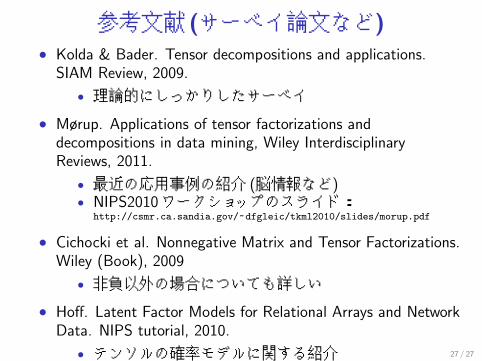
参考文献 (サーベイ論文など)• Kolda & Bader. Tensor decompositions and applications.
SIAM Review, 2009.
• 理論的にしっかりしたサーベイ• Mørup. Applications of tensor factorizations and
decompositions in data mining, Wiley InterdisciplinaryReviews, 2011.
• 最近の応用事例の紹介 (脳情報など)• NIPS2010ワークショップのスライド:
http://csmr.ca.sandia.gov/~dfgleic/tkml2010/slides/morup.pdf
• Cichocki et al. Nonnegative Matrix and Tensor Factorizations.Wiley (Book), 2009
• 非負以外の場合についても詳しい• Hoff. Latent Factor Models for Relational Arrays and Network
Data. NIPS tutorial, 2010.
• テンソルの確率モデルに関する紹介 27 / 27
Exponential Family Tensor Factorization:A Probabilistic Model for
Heterogeneous Relational Data
K. Hayashi1 T. Takenouchi2 T. Shibata3 Y. Kamiya4
D. Kato4 K. Kunieda4 K. Yamada4 K. Ikeda3
1JSPS, The University of Tokyo
2Future University Hakodate
3Nara Institute of Science and Technology
4C&C Lab, NEC Corporation
November 14, 2012
1 / 36
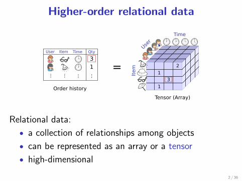
Higher-order relational data
Relational data:
• a collection of relationships among objects
• can be represented as an array or a tensor
• high-dimensional
2 / 36
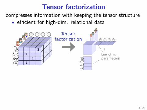
Tensor factorizationcompresses information with keeping the tensor structure
• efficient for high-dim. relational data
3 / 36
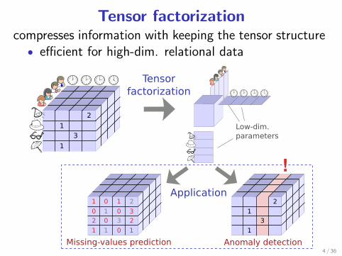
Tensor factorizationcompresses information with keeping the tensor structure
• efficient for high-dim. relational data
4 / 36
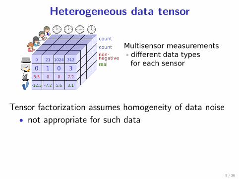
Heterogeneous data tensor
Tensor factorization assumes homogeneity of data noise
• not appropriate for such data
.Our approach..
......
generalize the tensor factorization, assuming a differentdistribution for each element [Hayashi+ ICDM’10][Hayashi+ KAIS]
5 / 36
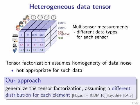
Heterogeneous data tensor
Tensor factorization assumes homogeneity of data noise
• not appropriate for such data.Our approach..
......
generalize the tensor factorization, assuming a differentdistribution for each element [Hayashi+ ICDM’10][Hayashi+ KAIS]
6 / 36
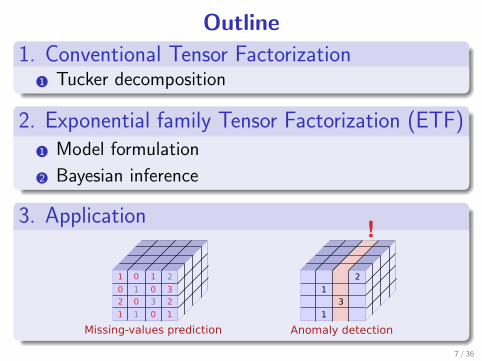
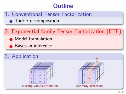
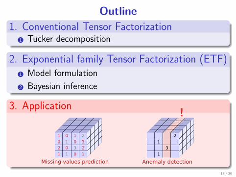
Outline.1. Conventional Tensor Factorization........ ..1 Tucker decomposition
.2. Exponential family Tensor Factorization (ETF)..
......
..1 Model formulation
..2 Bayesian inference
.3. Application..
......7 / 36
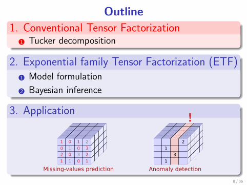
Outline.1. Conventional Tensor Factorization........ ..1 Tucker decomposition
.2. Exponential family Tensor Factorization (ETF)..
......
..1 Model formulation
..2 Bayesian inference
.3. Application..
......8 / 36
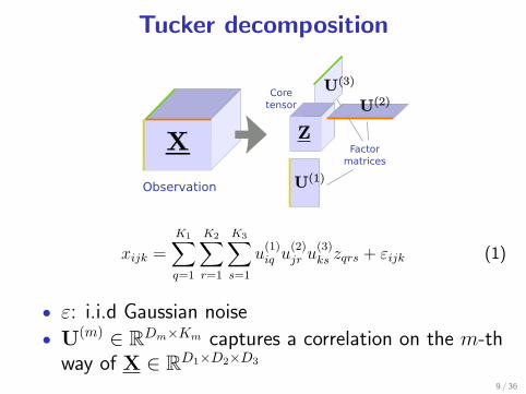
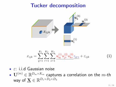
Tucker decomposition
xijk =
K1∑q=1
K2∑r=1
K3∑s=1
u(1)iq u
(2)jr u
(3)ks zqrs + εijk (1)
• ε: i.i.d Gaussian noise
• U(m) ∈ RDm×Km captures a correlation on the m-thway of X ∈ RD1×D2×D3
9 / 36
Tucker decomposition
xijk =
K1∑q=1
K2∑r=1
K3∑s=1
u(1)iq u
(2)jr u
(3)ks zqrs + εijk (1)
• ε: i.i.d Gaussian noise
• U(m) ∈ RDm×Km captures a correlation on the m-thway of X ∈ RD1×D2×D3
10 / 36
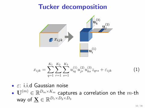
Tucker decomposition
xijk =
K1∑q=1
K2∑r=1
K3∑s=1
u(1)iq u
(2)jr u
(3)ks zqrs + εijk (1)
• ε: i.i.d Gaussian noise
• U(m) ∈ RDm×Km captures a correlation on the m-thway of X ∈ RD1×D2×D3
11 / 36
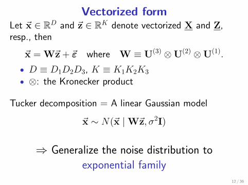
Vectorized formLet ~x ∈ RD and ~z ∈ RK denote vectorized X and Z,resp., then
~x = W~z + ~ε where W ≡ U(3) ⊗ U(2) ⊗ U(1).
• D ≡ D1D2D3, K ≡ K1K2K3• ⊗: the Kronecker product
Tucker decomposition = A linear Gaussian model
~x ∼ N(~x | W~z, σ2I)
⇒ Generalize the noise distribution to
exponential family12 / 36
Outline.1. Conventional Tensor Factorization........ ..1 Tucker decomposition
.2. Exponential family Tensor Factorization (ETF)..
......
..1 Model formulation
..2 Bayesian inference
.3. Application..
......13 / 36
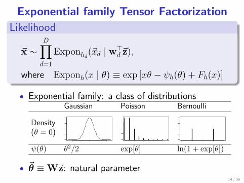
Exponential family Tensor Factorization.Likelihood..
......
~x ∼D∏
d=1
Exponhd(~xd | w>
d ~z),
where Exponh(x | θ) ≡ exp [xθ − ψh(θ) + Fh(x)]
• Exponential family: a class of distributionsGaussian Poisson Bernoulli
Density(θ = 0)
−4 −2 0 2 4
0.0
0.2
0.4
x
Den
sity
0 2 4 6 8
0.0
0.2
−0.5 0.0 0.5 1.0 1.5
0.3
0.5
0.7
ψ(θ) θ2/2 exp[θ] ln(1 + exp[θ])
• ~θ ≡ W~z: natural parameter14 / 36
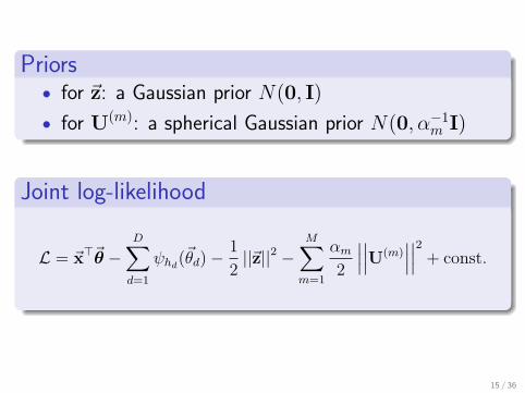
.Priors..
......
• for ~z: a Gaussian prior N(0, I)
• for U(m): a spherical Gaussian prior N(0, α−1m I)
.Joint log-likelihood..
......
L = ~x>~θ −D∑
d=1
ψhd(~θd) −
1
2||~z||2 −
M∑m=1
αm
2
∣∣∣∣∣∣U(m)∣∣∣∣∣∣2 + const.
15 / 36
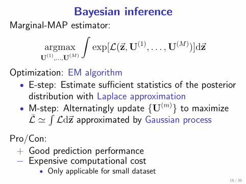
Bayesian inferenceMarginal-MAP estimator:
argmaxU(1),...,U(M)
∫exp[L(~z,U(1), . . . ,U(M))]d~z
Optimization: EM algorithm• E-step: Estimate sufficient statistics of the posterior
distribution with Laplace approximation• M-step: Alternatingly update {U(m)} to maximizeL̄ '
∫Ld~z approximated by Gaussian process
Pro/Con:+ Good prediction performance− Expensive computational cost
• Only applicable for small dataset16 / 36
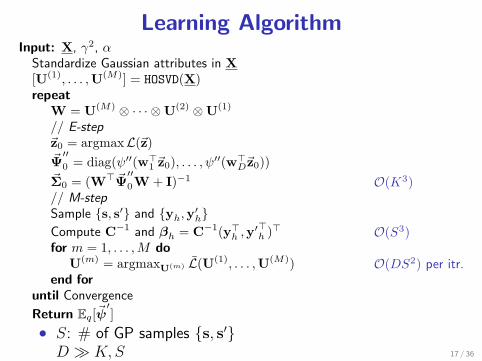
Learning AlgorithmInput: X, γ2, α
Standardize Gaussian attributes in X[U(1), . . . ,U(M)] = HOSVD(X)repeat
W = U(M) ⊗ · · · ⊗ U(2) ⊗ U(1)
// E-step~z0 = argmaxL(~z)~Ψ
′′0 = diag(ψ′′(w>
1 ~z0), . . . , ψ′′(w>D~z0))
~Σ0 = (W> ~Ψ′′0W + I)−1 O(K3)
// M-stepSample {s, s′} and {yh,y′
h}Compute C−1 and βh = C−1(y>
h ,y′>h )> O(S3)
for m = 1, . . . ,M doU(m) = argmaxU(m) L̄(U(1), . . . ,U(M)) O(DS2) per itr.
end foruntil Convergence
Return Eq[~ψ′]
• S: # of GP samples {s, s′}D À K,S 17 / 36
Outline.1. Conventional Tensor Factorization........ ..1 Tucker decomposition
.2. Exponential family Tensor Factorization (ETF)..
......
..1 Model formulation
..2 Bayesian inference
.3. Application..
......18 / 36
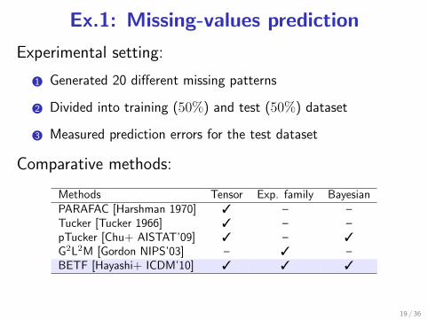
Ex.1: Missing-values prediction
Experimental setting:
..1 Generated 20 different missing patterns
..2 Divided into training (50%) and test (50%) dataset
..3 Measured prediction errors for the test dataset
Comparative methods:
Methods Tensor Exp. family BayesianPARAFAC [Harshman 1970] 3 – –Tucker [Tucker 1966] 3 – –pTucker [Chu+ AISTAT’09] 3 – 3G2L2M [Gordon NIPS’03] – 3 –BETF [Hayashi+ ICDM’10] 3 3 3
19 / 36
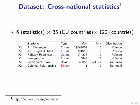
Dataset: Cross-national statistics1
• 6 (statistics) × 35 (EU countries)× 122 (countries)
Statistic Type Max Min DistributionX1 Air Passenger Count 19042009 0 PoissonX2 Air Freight & Mail Count 741055 0 PoissonX3 Railway Passenger Count 174217 0 PoissonX4 Immigration Count 6843 0 PoissonX5 Investment Flow Real 48853 -21190 GaussianX6 Colonial Relationship Binary 1 0 Bernoulli
1http://ec.europa.eu/eurostat20 / 36
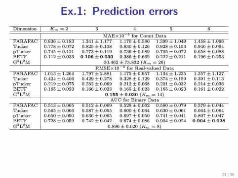
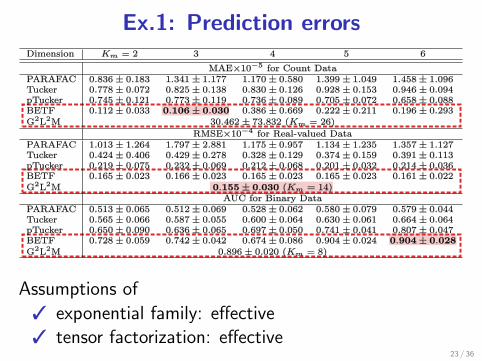
Ex.1: Prediction errors
3 exponential family: effective
3 tensor factorization: effective
21 / 36
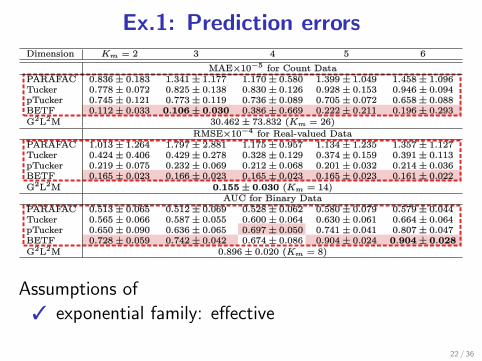
Ex.1: Prediction errors
Assumptions of
3 exponential family: effective
3 tensor factorization: effective
22 / 36
Ex.1: Prediction errors
Assumptions of
3 exponential family: effective3 tensor factorization: effective
23 / 36
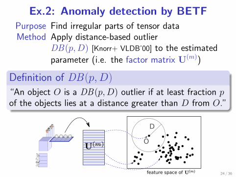
Ex.2: Anomaly detection by BETFPurpose Find irregular parts of tensor dataMethod Apply distance-based outlier
DB(p,D) [Knorr+ VLDB’00] to the estimatedparameter (i.e. the factor matrix U(m))
.Definition of DB(p,D)..
......
“An object O is a DB(p,D) outlier if at least fraction pof the objects lies at a distance greater than D from O.”
24 / 36
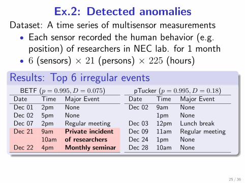
Ex.2: Detected anomaliesDataset: A time series of multisensor measurements
• Each sensor recorded the human behavior (e.g.position) of researchers in NEC lab. for 1 month
• 6 (sensors) × 21 (persons) × 225 (hours).Results: Top 6 irregular events..
......
BETF (p = 0.995, D = 0.075)Date Time Major EventDec 01 2pm NoneDec 02 5pm NoneDec 07 2pm Regular meetingDec 21 9am Private incident
10am of researchersDec 22 4pm Monthly seminar
pTucker (p = 0.995, D = 0.18)Date Time Major EventDec 02 9am None
1pm NoneDec 03 12pm Lunch breakDec 09 11am Regular meetingDec 24 1pm NoneDec 28 10am None
3 ETF detects anomaly events
25 / 36
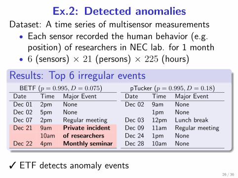
Ex.2: Detected anomaliesDataset: A time series of multisensor measurements
• Each sensor recorded the human behavior (e.g.position) of researchers in NEC lab. for 1 month
• 6 (sensors) × 21 (persons) × 225 (hours).Results: Top 6 irregular events..
......
BETF (p = 0.995, D = 0.075)Date Time Major EventDec 01 2pm NoneDec 02 5pm NoneDec 07 2pm Regular meetingDec 21 9am Private incident
10am of researchersDec 22 4pm Monthly seminar
pTucker (p = 0.995, D = 0.18)Date Time Major EventDec 02 9am None
1pm NoneDec 03 12pm Lunch breakDec 09 11am Regular meetingDec 24 1pm NoneDec 28 10am None
3 ETF detects anomaly events26 / 36
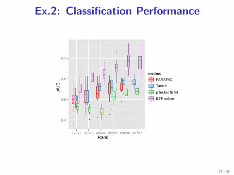
Ex.2: Classification Performance
Rank
AU
C
0.4
0.5
0.6
0.7
2x2x2 3x3x3 4x4x4 5x5x5 6x6x6 6x7x7
method
PARAFAC
Tucker
pTucker (EM)
ETF online
3 ETF well detect anomaly events
27 / 36
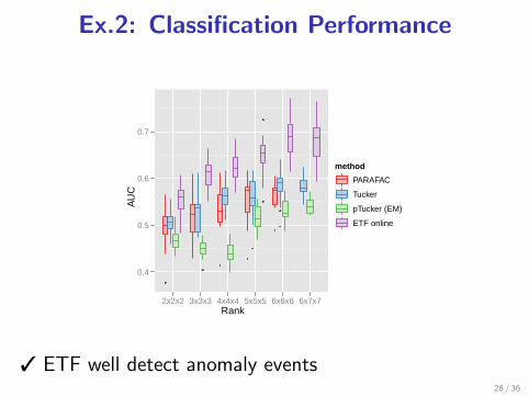
Ex.2: Classification Performance
Rank
AU
C
0.4
0.5
0.6
0.7
2x2x2 3x3x3 4x4x4 5x5x5 6x6x6 6x7x7
method
PARAFAC
Tucker
pTucker (EM)
ETF online
3 ETF well detect anomaly events28 / 36
.Summary..
......
..1 Proposed an integrative model for heterogeneouslyattributed data tensor
..2 Derived the Bayesian learning algorithm
..3 Showed the feasibility of the proposed method formissing-values prediction and anomaly detection
29 / 36
Appendix
30 / 36
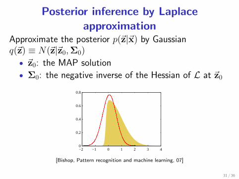
Posterior inference by Laplaceapproximation
Approximate the posterior p(~z|~x) by Gaussianq(~z) ≡ N(~z|~z0,Σ0)
• ~z0: the MAP solution
• Σ0: the negative inverse of the Hessian of L at ~z0
−2 −1 0 1 2 3 40
0.2
0.4
0.6
0.8
[Bishop, Pattern recognition and machine learning, 07]
31 / 36
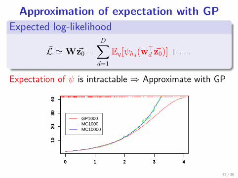
Approximation of expectation with GP.Expected log-likelihood..
......
L̄ ' W~z0 −D∑
d=1
Eq[ψhd(w>
d ~z0)] + . . .
Expectation of ψ is intractable ⇒ Approximate with GP
0 1 2 3 4
1020
3040
0 1 2 3 4
1020
3040
0 1 2 3 4
1020
3040
GP1000MC1000MC10000
32 / 36
Predictive mean and varianceSince ψ is the cumulant generating function,
ψ′(θ0) ≡dψ
dθ|θ0
= E[x|θ0], ψ′′(θ0) ≡d2ψ
dθ2 |θ0= var[x|θ0].
⇒ We can compute the mean and the variance of thepredictive distribution p(x|~x) by marginalizing ψ′(θ) andψ′′(θ) with the posterior of ~z and estimated W.
E[x|~x] ' Eq[ψ′(θ)], var[x|~x] ' Eq[ψ
′′(θ)]
We can analytically compute Eq[ψ′(θ)] and Eq[ψ
′′(θ)]with GP.
• Use Eq[ψ′(θ)] as an estimator of the missing value
33 / 36
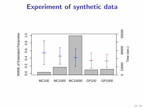
Experiment of synthetic data
MC100 MC1000 MC10000 GP100 GP1000
010
000
3000
050
000
Tim
e (s
ec.)
RM
SE
of E
stim
ated
Par
amet
er
0.0
0.2
0.4
0.6
0.8
1.0
34 / 36
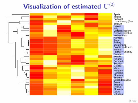
Visualization of estimated U(2)
35 / 36
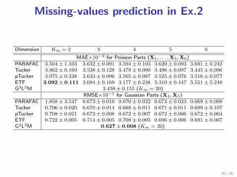
Missing-values prediction in Ex.2
Dimension Km = 2 3 4 5 6
MAE×10−3 for Poisson Parts (X1, . . . ,X3,X6)PARAFAC 3.504 ± 1.103 3.632 ± 0.091 3.594 ± 0.103 3.620 ± 0.093 3.691 ± 0.242Tucker 3.862 ± 0.169 3.538 ± 0.128 3.478 ± 0.090 3.496 ± 0.097 3.445 ± 0.096pTucker 3.975 ± 0.238 3.633 ± 0.096 3.565 ± 0.087 3.525 ± 0.076 3.516 ± 0.077ETF 3.092 ± 0.111 3.094 ± 0.169 3.177 ± 0.238 3.310 ± 0.447 5.551 ± 5.248G2L2M 3.438 ± 0.155 (Km = 20)
RMSE×10−1 for Gaussian Parts (X4,X5)PARAFAC 1.858 ± 3.547 0.673 ± 0.010 0.670 ± 0.022 0.674 ± 0.023 0.669 ± 0.009Tucker 0.706 ± 0.020 0.670 ± 0.014 0.668 ± 0.011 0.671 ± 0.011 0.699 ± 0.107pTucker 0.708 ± 0.021 0.673 ± 0.008 0.672 ± 0.007 0.672 ± 0.006 0.672 ± 0.004ETF 0.722 ± 0.005 0.714 ± 0.005 0.708 ± 0.005 0.696 ± 0.006 0.691 ± 0.007G2L2M 0.627 ± 0.008 (Km = 20)
36 / 36


![[2016-07-06] DDBJデータ解析チャレンジ概要](https://img.pdfslide.tips/doc/110x75/5870c1e21a28ab0b4a8b749f/2016-07-06-ddbj.jpg)