Embed Size (px)
Citation preview

J. Fluid Mech. (2010), vol. 665, pp. 418–456. c© Cambridge University Press 2010
doi:10.1017/S0022112010004003
Film flow over heated wavy inclined surfaces
S. J. D. D’ALESSIO1†, J. P. PASCAL2, H. A. JASMINE2
AND K. A. OGDEN1
1Department of Applied Mathematics, University of Waterloo, Waterloo, Ontario, Canada N2L 3G12Department of Mathematics, Ryerson University, Toronto, Ontario, Canada M5B 2K3
(Received 9 August 2009; revised 25 July 2010; accepted 26 July 2010;
first published online 27 October 2010)
The two-dimensional problem of gravity-driven laminar flow of a thin layer offluid down a heated wavy inclined surface is discussed. The coupled effect ofbottom topography, variable surface tension and heating has been investigatedboth analytically and numerically. A stability analysis is conducted while nonlinearsimulations are used to validate the stability predictions and also to studythermocapillary effects. The governing equations are based on the Navier–Stokesequations for a thin fluid layer with the cross-stream dependence eliminated bymeans of a weighted residual technique. Comparisons with experimental data anddirect numerical simulations have been carried out and the agreement is good. Newinteresting results regarding the combined role of surface tension and sinusoidaltopography on the stability of the flow are presented. The influence of heating andthe Marangoni effect are also deduced.
Key words: instability, Marangoni convection, thermocapillarity
1. IntroductionA shallow layer of fluid resting on a heated horizontal surface is known to become
unstable to both buoyancy-driven convection and thermocapillary convection. If thefluid layer is sufficiently thin thermocapillary convection, induced by gradients insurface tension, is expected to be the dominant instability mechanism. This is knownas the Marangoni effect. It has even been suggested (Smith 1966) that the instabilityobserved by Benard (1900) was likely due to the Marangoni effect rather than thebuoyancy effects. When the fluid layer is allowed to flow over an inclined heatedsurface the dynamics are controlled by several competing mechanisms. As noted byRuyer-Quil et al. (2005), first there is the classical long-wave instability resulting fromisothermal flows, which was originally studied experimentally by Kapitza & Kapitza(1949). The linear stability properties associated with this mode are now well knowndue to the work by Benjamin (1957) and Yih (1963) and the key finding is thatthe critical Reynolds number, Recrit , beyond which the flow becomes unstable, isgiven by Recrit = 5 cotβ/6, where β is the angle of inclination. This result has beenverified by the experiments of Liu, Paul & Gollub (1993) and a physical mechanism
† Email address for correspondence: [email protected]
Film flow over heated wavy inclined surfaces 419
for this long-wave instability was provided by Smith (1990). In addition, Goussis& Kelly (1991) have identified two other instability modes, which result from theMarangoni instability brought on by an inhomogeneous temperature field: a short-wave instability (Pearson 1958) and a long-wave instability (Scriven & Sternling 1964;Smith 1966).
The problem of thin-film flow over an even inclined heated surface was studiedby Kalliadasis, Kiyashko & Demekhin (2003b) and Kalliadasis et al. (2003a), andlater revisited by Ruyer-Quil et al. (2005), Scheid et al. (2005a) and Trevelyan et al.(2007). In these studies the focus was on the long-wave instability. A method tostudy the long-wave nature of the instability was devised by Benney (1966). Thismethod involves introducing a small long-wave parameter and carrying out anexpansion in this parameter, which ultimately leads to a single evolution equation,commonly referred to as the Benney equation, for the free surface. This procedure,along with similar approaches, has proved to be very successful in determining thethreshold of instability and has been thoroughly reviewed by Chang (1994). Theevolutionary equations for the free surface emerging from these techniques havebeen applied to numerous problems ranging from Newtonian to non-Newtonianfluids (Lin 1974; Nepomnyashchy 1974; Oron, Davis & Bankoff 1997; Usha &Uma 2004), isothermal to non-isothermal flows (Lin 1975; Scheid et al. 2005a; Joo,Davis & Bankoff 1991; Mukhopadhyay & Mukhopadhyay 2007; Samanta 2008),impermeable to porous surfaces (Thiele, Goyeau & Velarde 2009), even to unevenbottom topography (Tougou 1978; Davalos-Orozco 2007) and also combinationsthereof (Usha & Uma 2004; Khayat & Kim 2006; Thiele et al. 2009), to list a few.In addition, an extensive review of the dynamics and stability of thin-film flows hasrecently been prepared by Craster & Matar (2009). One serious drawback of theBenney equation lies in the fact that the solution becomes singular (i.e. it blowsup) in finite time shortly after criticality. Since solutions to the full Navier–Stokesequations do not display such a behaviour, the singularity present in the Benneyequation, as pointed out by Rosenau, Oron & Hyman (1992), Salamon, Armstrong& Brown (1994), Oron & Gottlieb (2004) and Scheid et al. (2005b), bears no physicalrelevance.
Situations involving falling films occur often in environmental and industrial settingsand continue to interest researchers. Because of this, considerable effort has beeninvested in modelling such flows. One class of models is known as integral-boundary-layer (IBL) models. The basic idea behind these models is first to simplify thegoverning Navier–Stokes equations by formulating them in terms of a shallownessparameter and neglecting terms that are deemed to be small. Next, the cross-streamdependence is eliminated by depth-integrating the equations and prescribing thevelocity variation with respect to depth. The standard choice is the parabolic velocityprofile, which follows from the laminar steady balance between gravity and viscosity.The original IBL model was developed by Shkadov (1967) and it was first-order sinceonly terms that are O(δ) were retained in the equations, where δ is the shallownessparameter. The IBL approach has been shown to accurately describe the flow in thenon-uniform and transient regime and also to capture the flow under supercriticalconditions (Alekseenko, Nakoryakov & Pokusaev 1985; Julien & Hartley 1986).Despite the success and attempts to improve them (Prokopiou, Cheng & Chang1991), IBL models are plagued with the serious flaw that they are unable to reproducethe critical conditions for the onset of instability as predicted by Orr–Sommerfeldcalculations and experiments (Kapitza & Kapitza 1949; Benjamin 1957; Yih 1963;Liu et al. 1993).

420 S. J. D. D’Alessio, J. P. Pascal, H. A. Jasmine and K. A. Ogden
The deficiency exhibited by IBL models has been remedied by Ruyer-Quil &Manneville (2000, 2002) using a weighted residual technique. The second-orderequations emerging from this method can be expressed as a system of two equationsgoverning the fluid depth, h, and the flow rate, q , and can be regarded as themodified IBL equations. The modified IBL model not only correctly predicts thethreshold for the onset of linear instability, but also provides an accurate descriptionof the nonlinear development of waves up to relatively high Reynolds numbers whencompared with the experimental observations of Liu, Schneider & Gollub (1995) andthe direct numerical simulations of Ramaswamy, Chippada & Joo (1996). The abilityof this model to accurately describe unstable flows far from criticality qualifies it as amajor improvement over the Benney equation which is only valid near criticality. Theweighted residual method appears to be gaining popularity as it has been successfullyapplied to other problems. For example, Ruyer-Quil et al. (2005) and Scheid et al.(2005a) have used it to study thermocapillary effects for the problem of film flow overan even inclined heated surface; Oron & Heining (2008) implemented it to investigatefilm flow falling down a corrugated vertical wall; and recently, D’Alessio, Pascal &Jasmine (2009) have generalized the method to model the flow down an unevenincline, to name a few.
The main purpose of the present investigation is to extend the thermocapillarystudies of Kalliadasis et al. (2003a, b), Ruyer-Quil et al. (2005), Scheid et al. (2005a)and Trevelyan et al. (2007) by accounting for bottom topography and hence widenthe range of applications. Both numerical and analytical methods have been utilizedto better understand how the complicated interplay between heating, strong surfacetension and bottom topography affect the stability of the flow. The underlyingassumptions made here are that the flow remains laminar and two-dimensional forall time, t . These conditions are expected to be satisfied if Re and cotβ are O(1).Although the governing equations will be derived for arbitrary bottom topography,we will focus our investigation on wavy inclines characterized by an amplitude anda wavelength. While the isothermal counterpart of this problem has been reportedin various numerical, analytical and experimental studies (Trifonov 1998, 2007a, b;Vlachogiannis & Bontozoglou 2002; Wierschem & Aksel 2003; Balmforth & Mandre2004; Wierschem, Lepski & Aksel 2005; Davalos-Orozco 2008; Hacker & Uecker2009; Heining & Aksel 2009; Heining et al. 2009), this study represents the first workto tackle the non-isothermal case.
The paper is structured as follows. In § 2, we derive a mathematical model todescribe the problem of laminar flow over a heated inclined surface having arbitrarybottom topography. The equations are expressed in terms of the fluid depth (h), flowrate (q) and surface temperature (θ) using a second-order weighted residual approach.As pointed out by D’Alessio et al. (2009), significant changes between first-order andsecond-order models can result. This is expected to be the case for non-isothermalflows as well and thus motivates the need to resort to a second-order model. Then,in § 3, a stability analysis is conducted for the case of sinusoidal bottom topography.Following this, nonlinear numerical simulations along with comparisons with existingdata and direct numerical simulations are presented in § 4. These results serve tovalidate the mathematical model as well as the analytical predictions, and also tostudy thermocapillary effects. Lastly, the key points are summarized in the concludingsection. Three appendices are also included. Appendix A is devoted to deriving theBenney equation corresponding to our problem. Appendix B lists various coefficientsappearing in the stability analysis in § 3 and Appendix C outlines the numericalsolution procedure used to obtain the results in § 4.

Film flow over heated wavy inclined surfaces 421
z, w
x, u
g
.
..............................................
..............................
..............................................
...........................
................................................
......................
................................................
...................
................................................
................
.................................................
............
..................................................
........
....................................................
....
......................................................
.
......................................................
.....................................................
....................................................
...................................................
..................................................
......................................................
..................................................
.................................................
.............
.....................................................
...................................................
..................................................
.................................................
................................................
..................................................
................................................
...
..............................................
.......
..............................................
.........
............................................
............
............................................
..............
............................................
................
..............................................................
BottomTb > Ta
Heatedliquid
h(x, t)
ζ(x)
h(x, t) + ζ(x)
Air, Ta
.........................................................................................................................
β
Figure 1. The flow configuration.
2. Governing equationsWe consider the two-dimensional laminar flow of a thin layer of a Newtonian fluid
along an uneven heated inclined surface, which is maintained at constant temperatureTb as shown in figure 1. The adopted (x, z) coordinate system is oriented so that thex-axis points along the incline, in the downhill direction, at an angle of β with thehorizontal, while the z-axis points in the upward normal direction. The bottom istaken to be periodic having the form
z = ζ (x) = Ab cos
(2πx
λb
), (2.1)
where Ab denotes the amplitude of the undulations and λb denotes the correspondingwavelength. The fluid velocity is denoted by u = (u, w)T.
We scale the equations as follows. For the vertical length scale, we choose theNusselt thickness, H , resulting from a flow rate, Q, which is given by
H =
(3µQ
ρg sin β
)1/3
, (2.2)
where g is the acceleration due to gravity, and ρ and µ are the fluid density andviscosity, respectively. The pressure is scaled using ρU 2, where U =Q/H is the velocityscale. The corresponding time scale is taken to be l/U , where l is the horizontallength scale which is taken to be λb. Lastly, the temperature is scaled according to�T = Tb − Ta , where Ta is the constant ambient air temperature and Tb > Ta .
While the fluid properties ρ, µ and the thermal diffusivity, κ , are assumed to remainconstant, the surface tension, σ , is allowed to vary with temperature, T , in the usualfashion,
σ (T ) = σ0 − γ (T − Ta), (2.3)
422 S. J. D. D’Alessio, J. P. Pascal, H. A. Jasmine and K. A. Ogden
where γ is a positive constant for most common fluids. Here, we have assumedthat the fluid layer is sufficiently thin so that buoyancy effects will be negligible.In addition, it is assumed that the liquid is non-volatile so that evaporation can beignored.
The governing two-dimensional Navier–Stokes and energy equations can then berendered in the following dimensionless form:
∂u
∂x+
∂w
∂z= 0, (2.4)
δReDu
Dt= −δRe
∂p
∂x+ 3 + δ2 ∂2u
∂x2+
∂2u
∂z2, (2.5)
δ2ReDw
Dt= −Re
∂p
∂z− 3 cotβ + δ3 ∂2w
∂x2+ δ
∂2w
∂z2, (2.6)
δRePrDT
Dt= δ2 ∂2T
∂x2+
∂2T
∂z2, (2.7)
where D/Dt denotes the two-dimensional material derivative, δ = H/l = H/λb is theshallowness parameter, Re =UH/ν is the Reynolds number, Pr = ν/κ is the Prandtlnumber and ν = µ/ρ is the kinematic viscosity.
We next assume that Re and Pr are of order unity and discard terms that are oforder δ3 in (2.4)–(2.7). Based on the result Recrit = 5 cotβ/6 for isothermal flow over aneven incline, we expect our assumption to be valid for sufficiently steep inclinationssince for sufficiently gentle inclinations cotβ will become of order 1/δ and thusmore terms in the equations will need to be retained. The equations then will be asfollows:
∂u
∂x+
∂w
∂z= 0, (2.8)
δReDu
Dt= −δRe
∂p
∂x+ 3 + δ2 ∂2u
∂x2+
∂2u
∂z2, (2.9)
δ2ReDw
Dt= −Re
∂p
∂z− 3 cotβ + δ
∂2w
∂z2, (2.10)
δRePrDT
Dt= δ2 ∂2T
∂x2+
∂2T
∂z2. (2.11)
The dynamic conditions at the free surface are (Nepomnyashchy, Velarde & Colinet2002):
p =2
ReF
(δ3
[∂z1
∂x
]2∂u
∂x+ δ
∂w
∂z− δ
∂z1
∂x
∂u
∂z− δ3 ∂z1
∂x
∂w
∂x
)− δ2(We − MaT )
F 3/2
∂2z1
∂x2,
(2.12)
− δMaRe√
F
(∂T
∂x+
∂z1
∂x
∂T
∂z
)= G
(∂u
∂z+ δ2 ∂w
∂x
)− 4δ2 ∂z1
∂x
∂u
∂x, (2.13)
−Bi√
FT =∂T
∂z− δ2 ∂z1
∂x
∂T
∂x. (2.14)
Here,
F = 1 + δ2
[∂z1
∂x
]2
and G = 1 − δ2
[∂z1
∂x
]2
, (2.15)

Film flow over heated wavy inclined surfaces 423
where z1 = ζ (x) + h(x, t) denotes the free surface, We = σ0H/(ρQ2) is the Webernumber, Ma = γ�T/(ρU 2H ) is the Marangoni number, Bi = αgH/(ρcpκ) is the Biotnumber with αg denoting the heat transfer coefficient across the liquid–air interfaceand cp is the specific heat at constant pressure of the liquid. We note that theseconditions are responsible for the coupling between the momentum and energyequations and that the surface-tension term is of second order or larger if the Webernumber is of order 1/δ or larger.
As before, to order δ2 these conditions yield:
p − 2δ
Re
∂w
∂z+ δ2(We − MaT )
∂2z1
∂x2= 0,
∂u
∂z− 4δ2 ∂z1
∂x
∂u
∂x+ δ2 ∂w
∂x+ MaReδ
(∂T
∂x+
∂z1
∂x
∂T
∂z
)= 0,
− BiT
(1 +
δ2
2
[∂z1
∂x
]2)
=∂T
∂z− δ2 ∂z1
∂x
∂T
∂x,
⎫⎪⎪⎪⎪⎪⎪⎪⎪⎪⎬⎪⎪⎪⎪⎪⎪⎪⎪⎪⎭
at z = z1. (2.16)
The kinematic condition dictating the position of the free surface is given by
w =∂h
∂t+ u
∂h
∂x+ uζ ′(x), (2.17)
and the scaled bottom profile is
ζ (x) = ab cos(2πx), where ab =Ab
H=
1
δ
Ab
λb
. (2.18)
In this study, we will consider small bottom waviness having Ab/λb of order δ andthus ab will be of order unity. At the interface between the fluid layer and theimpermeable bottom, the tangential and normal fluid velocity components are zero.This results in the no-slip and impermeability conditions
u = w = 0 at z = ζ (x). (2.19)
Finally, we have the bottom temperature condition
T = 1 at z = ζ (x). (2.20)
For small aspect ratio flows, which are slowly varying in the x direction, a depthaveraging of the equations is warranted. This removes the z-dependence from theproblem and yields a one-dimensional problem, which is better suited for mathematicalanalyses. By depth-integrating the continuity equation (2.8) and incorporating thekinematic condition, one obtains
∂h
∂t+
∂q
∂x= 0, (2.21)
where the flow rate, q , is given by
q =
∫ ζ (x)+h
ζ (x)
u dz. (2.22)
Integrating (2.10) from z = z1 = h + ζ to z and substituting the value for the pressureat the free surface from the first condition in (2.16) provides the following expression

424 S. J. D. D’Alessio, J. P. Pascal, H. A. Jasmine and K. A. Ogden
for the total pressure:
p =3 cotβ
Re(z1 −z)− δ
Re
∂u
∂x
∣∣∣∣z=z1
− δ
Re
∂u
∂x−δ2(We −MaT )
∂2z1
∂x2−δ2
∫ z
z1
Dw
Dtdz. (2.23)
This can be used to eliminate the pressure from the x-momentum equation (2.9). Itfollows that the inertia term in the above can be discarded owing to the factor of δ
multiplying the pressure gradient is (2.9), which makes it of order δ3 when Re is oforder unity.
Next, we implement the weighted residual technique to eliminate the z-dependence.This procedure begins by assuming the following profiles for the velocity andtemperature:
u =3q
2h3b +
δMaRe
4hb1
∂θ
∂x, (2.24)
T = 1 +(θ − 1)
h(z − ζ ), (2.25)
where b and b1 are given by
b = (z − ζ )(2h − z + ζ ), b1 = (z − ζ )(2h − 3z + 3ζ ), (2.26)
and are to be viewed as basis functions with respect to the z-coordinate. Here, wehave introduced the interfacial temperature θ(x, t) = T (x, z = z1, t). We note that theabove-assumed profile for u satisfies the no-slip condition u =0 at z = ζ and theleading-order free-surface condition
∂u
∂z= −δMaRe
∂θ
∂xat z = z1. (2.27)
Although the profile for T satisfies the bottom condition T = 1 on z = ζ , it doesnot satisfy the free-surface condition given by (2.16). In fact, it is impossible for theprofile to satisfy both. However, as noted by Kalliadasis et al. (2003a), the free-surfacecondition is incorporated into the energy equation when it is integrated over the fluidthickness, as described below.
In accordance with the Galerkin approach, we take b as the weight function andmultiply (2.9) by b and integrate with respect to z from ζ (x) to h + ζ (x). Likewise,for the energy equation we take the weight function to be (z − ζ ) and multiply (2.11)by this and again integrate from ζ (x) to h + ζ (x). After some algebra, we obtain thefollowing dimensionless equations for the flow variables h, q and θ:
∂h
∂t+
∂q
∂x= 0, (2.28)
∂q
∂t+
∂
∂x
[9
7
q2
h+
5
4
cotβ
Reh2 +
5
4Maθ
]
=q
7h
∂q
∂x+
5
2δRe
(h − q
h2
)+
5
6δ2Weh
(∂3h
∂x3+ ζ ′′′
)− 5 cotβ
2Reζ ′h +
δ
Re
×[
9
2
∂2q
∂x2− 9
2h
∂q
∂x
∂h
∂x+
4q
h2
(∂h
∂x
)2
− 6q
h
∂2h
∂x2− 5ζ ′q
2h2
∂h
∂x− 15ζ ′′q
4h− 5(ζ ′)2q
h2
]
+δReMa
16
[h2
3
∂2θ
∂x∂t+
15hq
14
∂2θ
∂x2+
19h
21
∂q
∂x
∂θ
∂x+
5q
7
∂h
∂x
∂θ
∂x
], (2.29)

Film flow over heated wavy inclined surfaces 425
h∂θ
∂t+
27q
20
∂θ
∂x− 7
40(1 − θ)
∂q
∂x
=3
δRePrh[1 − θ(1 + Bih)] +
δ
RePr
[(1 − θ)
∂2h
∂x2+ h
∂2θ
∂x2+
∂h
∂x
∂θ
∂x
−(
3Biθ
2+
2(1 − θ)
h
) (∂h
∂x
)2
− 3ζ ′(
(1 − θ)
h+ Biθ
)∂h
∂x+
3ζ ′′
2(1 − θ)
− 3Bi (ζ ′)2θ
2
]+
3δReMa
80
[2h2
(∂θ
∂x
)2
− h2(1 − θ)∂2θ
∂x2− 2h(1 − θ)
∂h
∂x
∂θ
∂x
]. (2.30)
In the isothermal limit, the above system reduces to the second-order modifiedIBL equations of D’Alessio et al. (2009) for an uneven bottom, and further settingζ ≡ 0 recovers the second-order modified IBL equations of Ruyer-Quil & Manneville(2000) for an even bottom. In arriving at these equations, we have assumed that theparameters Re, Ma, Bi, Pr and cotβ are all of order unity and that We is of order1/δ or larger.
3. Stability analysisTo examine how small disturbances will evolve when superimposed on a steady
equilibrium flow, we begin by first exploring the even bottom case and linearizeequations (2.28)–(2.30) using
h = 1 + h, q = 1 + q, θ =1
1 + Bi+ θ . (3.1)
Here, we have made use of the constant steady-state solutions hs = qs = 1 andθs =1/(1 + Bi ). We note from (2.28) that the steady-state solution for q is a constant.Thus, we select the scale for the flow rate, Q, such that q = qs = 1 in dimensionlessform. Next, we set
h = h0eikxeσ t , q = q0e
ikxeσ t , θ = θ0eikxeσ t , (3.2)
and combine the three equations. In order to make analytical progress, we only retainterms up to order δ to arrive at the following:
15δBiMak2
4RePr(1 + Bi )=
5δ
2Re(σ + 3ik)
(σ +
27
20ik
)+
3(1 + Bi )
RePr
[δσ
(σ +
17
7ik
)
+ δk2
(5 cotβ
2Re− 9
7
)+
5
2Re(σ + 3ik)
]. (3.3)
If σ = σr + iσi , then for neutral stability σr = 0. Substituting σ = iσi into the aboveand separating into real and imaginary parts, one finds σi = −3k resulting from theimaginary part which yields a dimensionless phase speed of c = −σi/k =3. When thisis substituted into the real part, the following instability threshold emerges:
Reevencrit =
10(1 + Bi )2 cotβ
5MaBi + 12(1 + Bi )2. (3.4)
We note that for arbitrary Ma the above expression recovers the isothermal resultwhen Bi = 0 or Bi → ∞ (although it must be remembered that we have assumed thatBi is of order unity). Moreover, it reveals that the Marangoni effect destabilizes theflow since Reeven
crit < 5 cotβ/6 for Ma > 0 (i.e. Tb > Ta). It can easily be shown that

426 S. J. D. D’Alessio, J. P. Pascal, H. A. Jasmine and K. A. Ogden
Reevencrit attains a minimum value of
Reevencrit,min =
40 cotβ
48 + 5Ma, (3.5)
when Bi =1. This destabilization of the flow was also obtained by Trevelyan et al.(2007) in their study of heated falling films using both specified heat flux and specifiedtemperature bottom boundary conditions. It is interesting to point out that when thereis no heat transfer across the liquid–air interface (i.e. Bi =0) the Marangoni effecthas no influence on the stability of the flow. This is easily explained by referring tothe steady-state temperature profile
Ts(z) = 1 − Biz
1 + Bi, (3.6)
and noting that when Bi = 0 a uniform temperature of Ts = 1 results and hencethermal effects disappear from the problem. The destabilization brought on by theMarangoni effect can be explained by considering a small sinusoidal perturbation onthe surface of the fluid layer. At the trough the temperature will be larger than atthe crest since it is closer to the heated bottom surface. Thus, surface tension will beweaker at the trough than at the crest resulting in a gradient in surface tension. This,in turn, will cause the fluid to be pulled away from the trough region to the crestregion and in doing so will accentuate the perturbation. Lastly, condition (3.4) canalso be obtained by considering the first-order Benney equation corresponding to ourproblem. These details are presented in Appendix A.
To determine how bottom topography alters the instability threshold, we analyse(2.28)–(2.30) using
h = hs(x) + h, q = 1 + q, θ = θs(x) + θ , (3.7)
where hs(x) and θs(x) denote the steady-state solutions to (2.29) and (2.30) and satisfy
5δ2We
6h3
sh′′′s − 6δ
Rehsh
′′s +
4δ
Re(h′
s)2 −
[5 cotβ
2Reh3
s +5δ
2Reζ ′ − 5δReMa
112h2
s θ′s − 9
7
]h′
s
− 15δ
4Reζ ′′hs − 5Ma
4θ ′sh
2s +
[15δReMa
224θ ′′s +
5
2δRe− 5 cotβ
2Reζ ′ +
5δ2We
6ζ ′′′
]h3
s
=5
2δRe+
5δ
Re(ζ ′)2, (3.8)
and(δ
RePr+
3δReMa
80hs(θs − 1)
)h2
s θ′′s +
[3δReMa
40hsh
′s(θs − 1) +
δ
RePrh′
s − 27
20
]hsθ
′s
+
[2δ
RePr(h′
s)2 − 3
δRePr(1 + Bihs) +
3δ
RePrζ ′h′
s − δ
RePr
(3
2ζ ′′ + h′′
s
)hs
− 3Biδ
2RePrhs(ζ
′ + h′s)
2
]θs +
3δReMa
40h3
s (θ′s)
2 = − 3
δRePr− δ
RePrhs
(3
2ζ ′′ + h′′
s
),
(3.9)
where the prime refers to differentiation with respect to x. Figures 2 and 3 show sometypical steady-state solutions for hs(x) and θs(x), respectively, whereas the free-surfaceand bottom contour profiles for this case are illustrated in figure 4. The flattening ofthe free surface with increasing surface tension is clearly visible. We observed little

Film flow over heated wavy inclined surfaces 427
0 0.1 0.2 0.3 0.4 0.5 0.6 0.7 0.8 0.9 1.00.80
0.85
0.90
0.95
1.00
1.05
1.10
1.15
1.20
1.25
x
hs
We = 10We = 100We = 500
Figure 2. Steady-state solution for hs(x) for the case Re = 0.5, cotβ = 0.5, δ = 0.1, ab = 0.2,Ma = 1, Bi =1 and Pr =7 for Weber numbers We = 10, 100, 500.
change in the steady-state solution for hs(x) and θs(x) when going from We = 500to We = 1000. Furthermore, the corresponding solutions for hs(x) for the isothermalcase were very similar to those shown with heating applied.
The linearized perturbation equations then become
∂h
∂t+
∂q
∂x= 0, (3.10)
∂q
∂t− 9δ
2Re
∂2q
∂x2+ f1
∂q
∂x+ f2q + f3h + f4
∂h
∂x+
6δ
Rehs
∂2h
∂x2− 5δ2We
6hs
∂3h
∂x3
− 5δReMa
112h′
s
∂θ
∂x− 15δReMa
224hs
∂2θ
∂x2− δReMa
48h2
s
∂2θ
∂x∂t= 0, (3.11)
∂θ
∂t+ g1
∂2θ
∂x2+ g2
∂θ
∂x+ g3θ +
27θ ′s
20hs
q + g4h − 7(1 − θs)
40hs
∂q
∂x+ g5
∂h
∂x− δ(1 − θs)
RePrhs
∂2h
∂x2= 0,
(3.12)
where the coefficients f1(x) − f4(x), g1(x) − g5(x) in (3.11) and (3.12) are listed inAppendix B. For periodic bottom topography, these coefficients will also be periodicfunctions. This permits the use of Floquet–Bloch theory to conduct the stabilityanalysis. We thus represent the perturbations as Bloch-type functions having the

428 S. J. D. D’Alessio, J. P. Pascal, H. A. Jasmine and K. A. Ogden
0 0.1 0.2 0.3 0.4 0.5 0.6 0.7 0.8 0.9 1.00.45
0.46
0.47
0.48
0.49
0.50
0.51
0.52
0.53
0.54
0.55
x
θs
We = 10We = 100We = 500
Figure 3. Steady-state solution for θs(x) for the case Re = 0.5, cotβ = 0.5, δ =0.1, ab = 0.2,Ma = 1, Bi = 1 and Pr = 7 for Weber numbers We = 10, 100, 500.
form
h = eσ teiKx
∞∑n=−∞
hnei2πnx, q = eσ teiKx
∞∑n=−∞
qnei2πnx, θ = eσ teiKx
∞∑n=−∞
θnei2πnx.
(3.13)
The exponential factor containing the Bloch wavenumber, K , represents disturbanceswhich interact with the periodic bottom topography via the equilibrium flow, which isrepresented by the Fourier series composed of its harmonics. Introducing the Bloch-type functions with truncated series into the perturbation equations reduces theequations to an algebraic problem, which can be solved numerically for the temporalgrowth rate �(σ ). In this way, we can determine the critical Reynolds number for theonset of instability, and for supercritical flows, we can compute the wavelength andspeed of unstable disturbances.
In order to reduce the parameter space to a manageable dimension, we have keptthe Prandtl number fixed at Pr = 7, which corresponds to water at room temperature.In most of our results, the Biot number was also fixed at Bi = 1. To establishthe impact of the remaining parameters Ma, We, cotβ, ab and δ on the stability ofthe flow for an uneven bottom, we start by presenting distributions of the criticalReynolds number, Recrit , with bottom amplitude for We = 10, 50, 450 in figures 5–7.These figures clearly reveal that Recrit depends on surface tension and this marksan important distinction in the stability characteristics between even and unevensurfaces, since for an even bottom Recrit is independent of We. Another interesting

Film flow over heated wavy inclined surfaces 429
1.2
1.0
0.8
0.6
0.4
0.2
0
0 0.1 0.2
bottom
free surface, We = 10free surface, We = 100
free surface, We = 500
0.3 0.4 0.5
x
z
0.6 0.7 0.8 0.9 1.0–0.2
Figure 4. Free surface and bottom contour for the case Re =0.5, cotβ = 0.5, δ = 0.1,ab = 0.2, Ma =1, Bi = 1 and Pr = 7 for Weber numbers We = 10, 100, 500.
feature, illustrated in figures 5–7, is that for the range 0 � ab � 0.5 the entire Recrit
distribution lies either above or below the value associated with the even bottom,Reeven
crit . Thus, for a fixed Weber number, the influence of bottom topography on thestability of the flow does not depend on the amplitude. It does, however, depend onMa and cotβ as portrayed in figures 5–7.
In figure 5, the complicated interaction between surface tension and bottomtopography is displayed for the case Ma =1 and cotβ = 1. We see that for We =10and We = 50 bottom topography plays a stabilizing role while for We = 450 it has adestabilizing influence. Increasing the Marangoni number to Ma = 5, shown in figure 6,we notice that for a fixed We the Recrit distribution lies below the corresponding onefor Ma = 1. This leads to the general conclusion that increasing Ma has a destabilizinginfluence as it was found for the even bottom case. On the other hand, we alsoobserve that for Ma = 5 bottom topography plays a stabilizing role, since for theWeber numbers presented the distribution lies above the value Reeven
crit , which is notthe case for Ma = 1. However, soon we will show that for Ma = 5 bottom topographyalso plays a destabilizing role if the Weber number is sufficiently large. Comparingfigures 5 and 7, it is seen that the influence that bottom topography has on thestability for large Weber numbers depends on the inclination. As the inclination isincreased, bottom topography has a stabilizing role for large-Weber-number flows.Lastly, the values of Recrit as ab → 0 in figures 5–7 are in excellent agreement with

430 S. J. D. D’Alessio, J. P. Pascal, H. A. Jasmine and K. A. Ogden
0 0.05 0.10 0.15 0.20 0.25 0.30 0.35 0.40 0.45 0.50
0.65
0.70
0.75
0.80
0.85
0.90
0.95
1.00
ab
Re c
rit
We = 10We = 50We = 450
Figure 5. Critical Reynolds number as a function of bottom amplitude withδ = 0.05, cotβ = 1, Ma = 1, Bi = 1 and Pr = 7.
those predicted by (3.4). As expected, these results are independent of We and thefigures clearly reveal this.
To establish the impact of heating and the Marangoni effect on the stability ofthe flow, in figure 8 we first present a plot of the critical Reynolds number versus theMarangoni number for We = 10, 50, 450. This diagram reaffirms the claim that theMarangoni effect appears to have a destabilizing influence on the flow. A similar plotof Recrit with Bi , which is shown in figure 9, demonstrates that there is a minimumat Bi = 1 as in the even bottom case.
In figures 10 and 11, we fix the bottom amplitude and set ab = 0.2. Since wehave discovered that surface tension influences the instability threshold, for ease ofinterpretation we have decided to plot (Reeven
crit −Recrit ) versus We for δ = 0.05, 0.07, 0.1with the understanding that (Reeven
crit − Recrit ) > 0 denotes a destabilizing effect onthe flow by bottom topography while (Reeven
crit − Recrit ) < 0 indicates that bottomtopography plays a stabilizing role. Values of We, where (Reeven
crit − Recrit ) = 0, can beregarded as transition points since the action of bottom topography as a stabilizingor destabilizing agent reverses as We passes through these values. Indeed, the reversalin stability as We increases is also evident from figure 5.
A reversal in the stabilizing action of bottom topography for the isothermal casehas been reported by D’Alessio et al. (2009) and Heining & Aksel (2009), and is alsoapparent in the results reported by Hacker & Uecker (2009). Heining & Aksel (2009)investigate the inverse problem, while Hacker & Uecker (2009) address the directproblem and express the equations of motion in terms of curvilinear coordinates

Film flow over heated wavy inclined surfaces 431
0 0.05 0.10 0.15 0.20 0.25 0.30 0.35 0.40 0.45 0.500.54
0.55
0.56
0.57
0.58
0.59
0.60
0.61
0.62
0.63
0.64
We = 10We = 50We = 450
Re c
rit
ab
Figure 6. Critical Reynolds number as a function of bottom amplitude withδ = 0.05, cotβ = 1, Ma = 5, Bi = 1 and Pr =7.
relative to the bottom profile. As was done by D’Alessio et al. (2009), Hacker& Uecker (2009) then resort to the weighted residual approach and implement aGalerkin method with a single-function expansion; however, in doing so they utilizea more refined velocity profile as was proposed by Scheid, Ruyer-Quil & Manneville(2006). The effect of surface tension on the stability of the flow is not the focusof the investigation reported by Hacker & Uecker (2009), and only three differentvalues of the relevant parameter are considered. Nevertheless, examining the presentedcritical Reynolds number distributions with the bottom waviness, it is evident thata reversal in the stabilizing role played by bottom topography is indicated as thesurface-tension parameter is increased. It should be pointed out that in all of theseprevious investigations, only small to moderate surface tension is considered. Tothe best of our knowledge, the current work is the first investigation to consider alarge range (10 � We � 105) of surface-tension values, and to discover a complicatednon-monotonic variation of the critical Reynolds number with this parameter.
Figure 10, which contains results for the isothermal case, reveals that for small Wevalues bottom topography acts to stabilize the flow, while for sufficiently largeWe values the role played by surface tension reverses to a destabilizing one.In the intermediate range, there is strong dependence on We with large deflectionsof the curves from zero, indicating a significant influence of bottom topography onflow stability, particularly around the transition point. It should also be pointedout that, since Reeven
crit is independent of We, intervals of increase and decrease ofthe (Reeven
crit − Recrit ) curve correspond to intervals of decrease and increase of Recrit ,

432 S. J. D. D’Alessio, J. P. Pascal, H. A. Jasmine and K. A. Ogden
0 0.05 0.10 0.15 0.20 0.25 0.30 0.35 0.40 0.45 0.500.35
0.40
0.45
0.50
0.55
0.60
We = 10We = 50We = 450
Re c
rit
ab
Figure 7. Critical Reynolds number as a function of bottom amplitude withδ = 0.05, cotβ = 0.5, Ma = 1, Bi = 1 and Pr = 7.
respectively. So, the turning (or stationary) points on these curves signal a reversal inthe stabilizing (or destabilizing) role played by surface tension.
The effect of decreasing δ, as can be seen in figure 10, is to increase the Wevalue of the transition point. Now, based on our scaling, decreasing δ can beassociated with increasing the wavelength of the bottom topography. Hence wecan infer that for longer bottom undulations stronger surface tension is neededto effectuate the more significant coupling between surface tension and bottomunevenness. The (Reeven
crit − Recrit ) curves corresponding to the non-isothermal casepresented in figure 11 have the same general shape as their isothermal counterparts,with the same number of transition and turning points. A close examination, however,reveals that heating increases the value of the transition Weber number and diminishesthe effect that bottom topography has on the stability of the flow for the entire Werange.
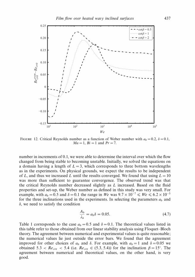
In figure 12, we present the (Reevencrit − Recrit ) distributions with We for various cotβ
values with δ = 0.1. It can be seen that as cot β is increased a larger portion of thedistribution lies above zero, which points to the fact that decreasing the inclinationaccentuates the destabilizing influence of bottom topography. Figure 13 shows a plotof (Reeven
crit − Recrit ) versus We for ab = 0.1, 0.2, 0.4. All the curves have approximatelythe same transition point. There is, however, a difference in the deviations from Reeven
crit :the smaller the bottom amplitude the smaller the deviations. Lastly, we present theRecrit distribution with ab for Ma = 1, 5 in figure 14. The curves indicate that in thepresence of sufficiently strong surface-tension thermocapillary effects can cause an

Film flow over heated wavy inclined surfaces 433
0.5 1.0 1.5 2.0 2.5 3.0 3.5 4.0 4.5 5.00.55
0.60
0.65
0.70
0.75
0.80
0.85
Ma
Re c
rit
We = 10We = 50We = 450
Figure 8. Critical Reynolds number as a function of Marangoni number with ab = 0.2,δ = 0.05, cotβ = 1, Bi = 1 and Pr = 7.
abrupt change in the critical Reynolds number. Indeed, a reversal in stability occurswhen the Marangoni number is increased from Ma = 1 to Ma = 5 as a result ofbottom unevenness coupled with strong surface tension. One last observation worthnoting regards the profile of the steady-state free surface in relation to that of thebottom. For small Weber numbers, apart from a vertical shift, the free-surface profilemirrors that of the bottom. However, as We increases the two profiles become out ofphase. In fact, the shift between profiles seems to develop near the occurrence of thereversal in stability. As We increases further the free surface becomes flatter but stillnoticeably out of phase with the bottom. This behaviour was observed in all casesand is apparent in figure 4.
As a final plot, figure 15 presents neutral stability curves in the K − Re planefor different bottom amplitudes and Marangoni numbers. The interesting featureobserved here is that for small ab the critical wavenumber occurs at K = 0. That is,perturbations having an infinitely long wavelength are the most unstable. However,for larger ab the critical wavenumber moves away from K = 0, and the neutralstability curve takes on a significantly different shape. As evident from the diagram,the Marangoni number also influences the shape of the curve.
In the next section, we present numerical simulations and comparisons to validateour modelling equations and also to verify some of the predictions made in thissection. Because of the lack of experimental data available for heated falling films,our focus will be on isothermal flows.

434 S. J. D. D’Alessio, J. P. Pascal, H. A. Jasmine and K. A. Ogden
0 0.2 0.4 0.6 0.8 1.0 1.2 1.4 1.6 1.8 2.00.72
0.74
0.76
0.78
0.80
0.82
0.84
0.86
0.88
Bi
Re c
rit
We = 10We = 50We = 450
Figure 9. Critical Reynolds number as a function of Biot number with ab = 0.2, δ =0.05,cotβ =1, Ma = 1 and Pr = 7.
4. Results, comparisons and discussionsThe instability of a particular equilibrium flow can be determined by gauging
the evolution initiated by small disturbances. The development of the flow canbe calculated by numerically solving the fully nonlinear governing equations. Theadvantage of this approach is that it incorporates nonlinear interactions of theperturbations and thus captures the entire instability mechanism of the flow.Furthermore, for unstable flows, the temporal evolution can be continued untilthe growth of the disturbances reaches saturation with the solution then revealingthe structure of the subsequent secondary flow. Using this numerical approach toperform a nonlinear stability analysis has been successful in related previous studies(Kranenburg 1992; Brook, Pedley & Falle 1999; Chang, Demekhin & Kalaidin 2000;Zanuttigh & Lamberti 2002; Balmforth & Mandre 2004; D’Alessio et al. 2009).
We employed the numerical method described in Appendix C to solve the governingunsteady equations (2.28)–(2.30) on a periodic spatial domain of length L, where L
is some multiple of the bottom wavelength. The evolution of the unsteady flow wascomputed using the perturbed steady-state solutions as initial conditions. Since thecomputational domain length, L, forces the largest wavelength (smallest wavenumber)of the perturbation to be L (wavenumber 2π/L), we can thus exploit this featureto determine the critical Reynolds number for which the flow becomes unstable byvarying Re for a fixed L using a perturbation of wavelength L. Using this strategy,we ran numerous numerical simulations to identify points on the neutral stability

Film flow over heated wavy inclined surfaces 435
101 102 103 104 105−0.2
–0.1
0
0.1
0.2
0.3
0.4
0.5
We
Re
even
−R
e cri
t
δ = 0.05δ = 0.075δ = 0.1
crit
Figure 10. Critical Reynolds number as a function of Weber number with ab =0.2,cotβ =1 for the isothermal case.
curve. Figure 16 shows a comparison in the K − Re plane between these points andthe theoretical curve obtained using the linear analysis of the previous section. Thefigure displays close agreement between the nonlinear simulations and linear theory.
We next make comparisons with experimental data and begin with the isothermalcase over an even bottom. For this, we refer to the experiments conducted by Liu et al.(1995) using glycerin–water films at an inclination of β =4.0◦. The fluid propertiescorresponding to their set-up are as follows:
ν = 2.3 × 10⁻⁶ m2
s, ρ = 1.07 × 10³ kg
m3, σ0 = 6.7 × 10⁻² N
m. (4.1)
Their data consist of points on the neutral stability curve in the f − Re plane, wheref denotes the cutoff frequency. The following expression for the neutral stabilitycurve can easily be derived using a linear stability analysis and is given by
5
6
cotβ
Re=
175 + 5(δk)2 − 33(δk)4
7[5 + 9(δk)2]2− 5
18We(δk)2. (4.2)
Figure 17 illustrates a comparison between the two in the δk − Re plane, where δk
and f are related through
f =
(g sinβ
3
)2/3 (Re
ν
)1/3cδk
2π. (4.3)
The critical Reynolds numbers from the experimental data have been scaled by 2/3so as to conform with our definition of Re. In arriving at the above expression, we

436 S. J. D. D’Alessio, J. P. Pascal, H. A. Jasmine and K. A. Ogden
−0.2
–0.1
0
0.1
0.2
0.3
0.4
0.5
δ = 0.05δ = 0.075δ = 0.1
101 102 103 104 105
We
Re
even
−R
e cri
tcr
it
Figure 11. Critical Reynolds number as a function of Weber number with ab = 0.2, cotβ = 1,Ma =5, Bi = 1 and Pr = 7.
have made use of the scaling introduced earlier with c denoting the dimensionlessphase speed and f is in Hz. Since the fluid is specified the Weber number in (4.2) canbe expressed as
We =
(3
sinβ
)1/3Ka
Re5/3, (4.4)
where Ka = σ0/(ρg1/3ν4/3) denotes the Kapitza number. Since Ka depends only onthe fluid properties it has a numerical value of Ka = 963.45. Figure 17 displays verygood agreement between experimental and theoretical values.
For the isothermal case of an uneven bottom, the only experimental data availableare those of Wierschem et al. (2005). The fluid used in their experiments is a siliconeoil (B200) having the following fluid properties:
ν = 2.24 × 10⁻⁴ m2
s, ρ = 9.68 × 10² kg
m3, σ0 = 2.07 × 10⁻² N
m. (4.5)
The experimental apparatus had a wavy bottom consisting of three equal sinusoidalwaves having
Ab
λb
= 0.05. (4.6)
Table 1 shows a comparison between the experimental, numerical and theoreticalRecrit values. The numerical results were obtained by solving our nonlinear modelequations with a disturbance of wavelength L added to the steady-state solutions.By monitoring the growth or decay of the disturbance and stepping the Reynolds
Film flow over heated wavy inclined surfaces 437
−0.15
−0.10
−0.05
0
0.05
0.10
0.15
0.20
0.25
cotβ = 0.5cotβ = 1cotβ = 2
101 102 103 104 105
We
Reev
en−
Re c
rit
crit
Figure 12. Critical Reynolds number as a function of Weber number with ab = 0.2, δ =0.1,Ma = 1, Bi = 1 and Pr = 7.
number in increments of 0.1, we were able to determine the interval over which the flowchanged from being stable to becoming unstable. Initially, we solved the equations ona domain having a length of L =3, which corresponds to three bottom wavelengthsas in the experiments. On physical grounds, we expect the results to be independentof L, and thus we increased L until the results converged. We found that using L =10was more than sufficient to guarantee convergence. The observed trend was thatthe critical Reynolds number decreased slightly as L increased. Based on the fluidproperties and set-up, the Weber number as defined in this study was very small. Forexample, with ab = 0.5 and δ = 0.1 the range in We was 9.7 × 10⁻⁷ � We � 6.2 × 10⁻⁵
for the three inclinations used in the experiments. In selecting the parameters ab andδ, we need to satisfy the condition
Ab
λb
= abδ = 0.05. (4.7)
Table 1 corresponds to the case ab = 0.5 and δ = 0.1. The theoretical values listed inthis table refer to those obtained from our linear stability analysis using Floquet–Blochtheory. The agreement between numerical and experimental values is quite reasonable;the numerical values lie just outside the error bars. We found that the agreementimproved for other choices of ab and δ. For example, with ab = 1 and δ = 0.05 weobtained 5.3 < Recrit < 5.4 (i.e. Recrit ∈ (5.3, 5.4)) for the inclination β = 15◦. Theagreement between numerical and theoretical values, on the other hand, is verygood.

438 S. J. D. D’Alessio, J. P. Pascal, H. A. Jasmine and K. A. Ogden
Recrit
β Reevencrit Experimental Numerical Theoretical
15◦ 3.1 5.1 ± 0.4 (5.5, 5.6) 5.630◦ 1.4 2.2 ± 0.2 (1.8, 1.9) 1.740.7◦ 0.97 1.3 ± 0.1 (1.1, 1.2) 1.1
Table 1. Comparison between experimental, numerical and theoretical values of Recrit forthe isothermal case having ab = 0.5 and δ = 0.1.
−0.2
−0.1
0
0.1
0.2
0.3
0.4
0.5
ab = 0.1
ab = 0.2
ab = 0.4
101 102 103 104 105
We
Reev
en−
Re c
rit
crit
Figure 13. Critical Reynolds number as a function of Weber number with δ = 0.1, cotβ = 1,Ma =1, Bi = 1 and Pr = 7.
Here, Reevencrit = 5 cotβ/6 refers to the critical Reynolds number for the even bottom
case and is included to illustrate the stabilizing influence of bottom topography.Lastly, we note that the critical Reynolds numbers presented in the experimentalinvestigation of Wierschem et al. (2005) were multiplied by 2/3 in order to complywith our definition of Re.
Numerical simulations, as outlined above, were also used to confirm the reversals instability as predicted by linear theory. For example, linear theory predicts that for theisothermal case having ab = 0.5, δ = 0.1 and cotβ = 0.5, Recrit > Reeven
crit when We = 10,while Recrit < Reeven
crit when We = 100. With Re =Reevencrit , numerical simulations revealed
that disturbances decayed in time when We = 10 and grew in time when We =100.

Film flow over heated wavy inclined surfaces 439
0 0.05 0.10 0.15 0.20 0.25 0.30 0.35 0.40 0.45 0.500.26
0.28
0.30
0.32
0.34
0.36
0.38
ab
Re c
rit
Ma = 1
Ma = 5
Figure 14. Critical Reynolds number as a function of bottom amplitude with δ = 0.05,cotβ = 0.5, We = 900, Bi = 1 and Pr = 7.
Next, we make comparisons with direct numerical simulations utilizing the softwarepackage CFX. This program solves the Navier–Stokes equations, expressed in termsof the primitive variables u, v, w and p, using a combination of the finite volumeand finite element methods. The domain is discretized into fluid elements and controlvolumes are formed around element nodes with momentum and mass being conservedover each control volume. Flow variables and fluid properties are stored at the nodes,which are located within each control volume. The finite element method, using shapefunctions, is employed to calculate properties within fluid elements at the edges ofthe control volumes. An advection discretization scheme is used which is a boundedsecond-order upwind scheme. To locate the free surface, a volume-of-fluid method isused. The volume fraction of fluid is tracked as a solution variable using a volumefraction advection scheme. This causes a smearing of the interface due to numericaldiffusion; however, CFX uses a compressive scheme to minimize this diffusion. Theinterface location in this study was chosen as the contour along which the volumefractions of water and air are each 0.5.
In our two-dimensional simulations, a domain length of 20 bottom wavelengths(i.e. L = 20) was chosen with periodic boundary conditions applied at the ends, andsteady-state solutions used as initial conditions. We have found that the progression ofan unstable flow mimics the general phases observed in isothermal film flows (Chang,1994), and shallow flows along even (Brock 1969; Julien & Hartley 1986) and uneven(D’Alessio et al. 2009) surfaces. Figure 18 presents comparisons between our modeland CFX simulations for a supercritical isothermal case at a dimensionless time

440 S. J. D. D’Alessio, J. P. Pascal, H. A. Jasmine and K. A. Ogden
4.0 4.5 5.0 5.5 6.0 6.5 7.0 7.50
1
2
3
4
5
6
Re
K
ab = 0.4, Ma = 1
ab = 0.4, Ma = 0.1
ab = 0.2, Ma = 0.1
ab = 0.2, Ma = 1
Figure 15. Neutral stability curves for the case δ = 0.05, cotβ = 5, We =5, Bi = 1 and Pr = 7.
of t = 137. In terms of dimensional units, the flow set-up for the CFX simulationscorresponds to a configuration having a bottom wavelength of λb = 1 mm andamplitude Ab = 0.01 mm and Nusselt thickness H =0.1 mm. The figure shows thatwith the passage of time an initially constant distribution for q eventually settles intoa permanent wave profile consisting of three peaks. The agreement between the twosimulations is good; our model is able to correctly predict the essential features. Theonly noticeable difference is in the spacing between the peaks. Similar agreement inthe free-surface profile is also found. We observe that apart from the three prominentwaves the free-surface variations appear to be in phase with the bottom undulations,as previously noted for cases with weak surface tension.
As a final simulation, we consider a non-isothermal supercritical case withmoderately strong surface tension. Figures 19–21 present plots obtained from ourmodel equations. Figure 19 shows how a perturbed initial steady-state solution evolvesin time to form a permanent solitary wave structure. In figure 20, the correspondingdistributions for the fluid thickness, h, and fluid surface temperature, θ , are plottedat t = 200. We observe that the surface temperature distribution is out of phase withthat of h indicating that a thinner fluid layer results in a larger surface temperature.This can be reasoned by examining the steady-state temperature profile given by
Ts(x, z) = 1 − Bi
(1 + Bi )hs(x)(z − ζ (x)). (4.8)

Film flow over heated wavy inclined surfaces 441
0.35 0.40 0.45 0.50 0.55 0.60 0.65 0.70 0.75 0.800
0.5
1.0
1.5
2.0
2.5
3.0
3.5
Re
K
LinearNonlinear
Unstable
Stable
Figure 16. Neutral stability curve for the case ab = 0.1, δ = 0.1, cotβ = 0.5, We = 10, Ma =1,Bi = 1 and Pr = 7.
10 15 20 25 30 35 40 45 500
0.1
0.2
0.3
0.4
0.5
Re
kδ
TheoreticalExperimental data
Figure 17. Comparison between experimental and theoretical neutral stability curves for theisothermal case with ab = 0, β = 4.0◦ and Ka = 963.45.

442 S. J. D. D’Alessio, J. P. Pascal, H. A. Jasmine and K. A. Ogden
2 4 6 8 10 12 14 16 18 200
2 4 6 8 10 12 14 16 18 200
2
4
6
(a)
(b)
(c)
(d )
q
2
4
6
q
Model q
CFX q
2 4 6 8 10 12 14 16 18 20
2 4 6 8 10 12 14 16 18 20
0
1
2
3
z
0
1
2
3
z
Model free surfaceBottom
x
CFX free surfaceBottom
Figure 18. Comparison in the permanent q and free-surface profiles for the isothermal casewith Re = 2.28, cotβ = 1.5, We = 0, ab = 0.1 and δ = 0.1 on a computational domain of lengthL =20.
This shows that the temperature decreases from the bottom surface at a uniformrate, which depends only on the heat transfer coefficient, Bi , and we expect a similarbehaviour to occur for the unsteady case as well. Lastly, figure 21 displays the free-surface profile at t = 200, which illustrates how the free-surface variations become outof phase with the bottom topography in the presence of sufficiently strong surfacetension.
In an attempt to understand the interaction between bottom topography andsurface tension, we begin by constructing an approximate steady-state solution of thetwo-dimensional equations (2.4)–(2.6). Since we have demonstrated that the reversalsin stability occur with or without heating, for simplicity we consider the isothermalcase. We start by expanding the steady-state flow variables us, ws, ps and hs in the

Film flow over heated wavy inclined surfaces 443
0 1 2 3 4 5 6 7 8 9 100.8
0.9
1.0
1.1
1.2
1.3
1.4
1.5
x
q
t = 75
t = 100
t = 200
Figure 19. Evolution of the q distribution for the case with Re = 1, cotβ = 0.5, Bi = 1,Ma = 1, We = 100, ab = 0.2, δ = 0.1 and Pr = 7 on a computational domain of length L = 10.
following series:
us(x, z) = u0(x, z) + δu1(x, z) + δ2u2(x, z) + · · · ,
ws(x, z) = w0(x, z) + δw1(x, z) + δ2w2(x, z) + · · · ,
ps(x, z) = p0(x, z) + δp1(x, z) + δ2p2(x, z) + · · · ,
hs(x) = 1 + δh1(x) + δ2h2(x) + · · · .
⎫⎪⎪⎪⎪⎬⎪⎪⎪⎪⎭
(4.9)
These expansions are then substituted into the steady-state versions of (2.4)–(2.6) andequating powers of δ results in a closed system of equations at each order. The sameis done for the corresponding boundary conditions (2.16) and (2.19).
Although this procedure is similar to that used in deriving the Benney equationdiscussed in Appendix A, there are some significant differences. For example, theBenney equation represents an unsteady evolution equation for h, which emanatesfrom the kinematic condition, whereas in the above approach the kinematic conditionis not used. In fact, in our formulation of the problem the approximate steady-statesolution for hs can be found a priori by substituting the expansion for hs into
5δ2We
6h3
s h′′′s − 6δ
Rehsh
′′s +
4δ
Re(h′
s)2 −
[5 cotβ
2Reh3
s +5δ
2Reζ ′ − 9
7
]h′
s − 15δ
4Reζ ′′hs
+
[5
2δRe− 5 cotβ
2Reζ ′ +
5δ2We
6ζ ′′′
]h3
s =5
2δRe+
5δ
Re(ζ ′)2. (4.10)
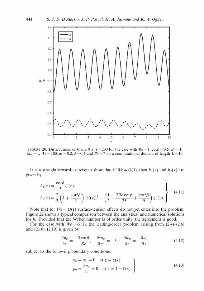
444 S. J. D. D’Alessio, J. P. Pascal, H. A. Jasmine and K. A. Ogden
0 1 2 3 4 5 6 7 8 9 100.4
0.5
0.6
0.7
0.8
0.9
1.0
1.1
1.2
1.3
1.4
x
h, θ
hθ
Figure 20. Distributions of h and θ at t =200 for the case with Re = 1, cotβ = 0.5, Bi = 1,Ma = 1, We = 100, ab = 0.2, δ = 0.1 and Pr = 7 on a computational domain of length L = 10.
It is a straightforward exercise to show that if We = O(1), then h1(x) and h2(x) aregiven by
h1(x) =cotβ
3ζ ′(x),
h2(x) =2
3
(1 +
cot2β
3
)[ζ ′(x)]2 +
(1
2− 2Re cotβ
35+
cot2β
9
)ζ ′′(x).
⎫⎪⎪⎬⎪⎪⎭ (4.11)
Note that for We =O(1) surface-tension effects do not yet enter into the problem.Figure 22 shows a typical comparison between the analytical and numerical solutionsfor hs . Provided that the Weber number is of order unity, the agreement is good.
For the case with We = O(1), the leading-order problem arising from (2.4)–(2.6)and (2.16), (2.19) is given by
∂p0
∂z= −3 cotβ
Re,
∂2u0
∂z2= −3,
∂w0
∂z= −∂u0
∂x, (4.12)
subject to the following boundary conditions:
u0 = w0 = 0 at z = ζ (x),
p0 =∂u0
∂z= 0 at z = 1 + ζ (x).
⎫⎬⎭ (4.13)

Film flow over heated wavy inclined surfaces 445
0 1 2 3 4 5 6 7 8 9 10−0.2
0
0.2
0.4
0.6
0.8
1.0
1.2
1.4
x
z
Bottom
Free surface
Figure 21. Free-surface variations at t = 200 for the case with Re = 1, cotβ =0.5, Bi = 1,Ma = 1, We = 100, ab = 0.2, δ = 0.1 and Pr = 7 on a computational domain of length L = 10.
The solutions are easily found to be
p0(x, z) =3 cotβ
Re(1 + ζ − z),
u0(x, z) = − 32(z − ζ )2 + 3(z − ζ ),
w0(x, z) = − 32ζ ′(z − ζ )2 + 3ζ ′(z − ζ ).
⎫⎪⎪⎪⎬⎪⎪⎪⎭
(4.14)
We note that although the kinematic condition was not imposed in arriving at theabove solutions, w0(x, z) does, in fact, satisfy the free-surface condition w0(x, z =1 +ζ ) = u0(x, z = 1 + ζ )ζ ′. Continuing this procedure and transferring the free-surfacecondition from z = hs(x) + ζ to z = 1 + ζ , we obtain
u1(x, z) = cotβζ ′ ( 32(z − ζ )2 − 2(z − ζ )
),
u2(x, z) = ζ ′′ ([ 12(z − ζ )2 − 2
3(z − ζ )
]cot2β − (z − ζ )3 + 3(z − ζ )2 − 3(z − ζ )
)− ζ ′′Re cotβ
(140
(z − ζ )6 − 320
(z − ζ )5 + 14(z − ζ )4 − 8
35(z − ζ )
)+
(ζ ′)2 (
3(z − ζ )2 − 4(z − ζ ) − 718
cot2β(z − ζ )).
⎫⎪⎪⎪⎪⎪⎬⎪⎪⎪⎪⎪⎭(4.15)

446 S. J. D. D’Alessio, J. P. Pascal, H. A. Jasmine and K. A. Ogden
0 0.1 0.2 0.3 0.4 0.5 0.6 0.7 0.8 0.9 1.00.95
0.96
0.97
0.98
0.99
1.00
1.01
1.02
1.03
1.04
1.05
x
hs
NumericalAnalytical
Figure 22. Comparison between analytical and numerical solutions for hs(x) for theisothermal case with ab = 0.2, cotβ = 0.5, Re = 1, We = 1 and δ = 0.1.
Equipped with this approximate solution for us(x, z), we are now prepared toexamine how bottom topography and surface tension affect the stability of the flow.Evaluating us on the free surface and averaging over the bottom topography, weobtain
us ≈ 32
−(2 + 7
9cot2β
)π2a2
bδ2. (4.16)
Defining
Us = us − 32
≈ −(2 + 7
9cot2β
)π2a2
bδ2 (4.17)
as the difference in the mean surface velocity between the uneven and even bottomcases, Us can be regarded as a mean surface drift resulting from bottom unevenness.This drift is a second-order effect which causes the steady-state flow to slow downslightly, which in turn will have a stabilizing effect. Thus, for negligible surface tension,bottom topography acts to retard the flow. Alternatively, we can interpret this in termsof the steady flow rate, Qs , where
Qs(x) =
∫ 1+ζ
ζ
us(x, z) dz, (4.18)
giving an average value of
Qs ≈ 1 −(2 + 7
18cot2β
)π2a2
bδ2. (4.19)
We see that a consequence of the mean surface drift is a slight reduction in the steadyflow rate, and hence mass transport.

Film flow over heated wavy inclined surfaces 447
For We = O(1), the influence of surface tension enters at higher order. Extendingthis analysis, we have found that the next non-zero term in the expansion for Qs
occurs at order δ4 and is given by
Qs ≈ 1 −(2 + 7
18cot2β
)π2a2
bδ2 + f (Re, ab, cotβ)δ4 − 76
27π4a2
bRe cotβWeδ4, (4.20)
where f (Re, ab, cotβ) denotes a complicated function that is independent of We. It isevident that for a fixed bottom configuration Qs decreases with We, which indicatesthat increasing surface tension stabilizes the flow. Furthermore, the magnitude of thegradient of the variation with We increases with ab, cotβ and δ. These predictionsare in agreement with those drawn from the linear stability analysis for We = O(1)as revealed by the results presented in figures 10–13; although the plots are shownfor We � 10, the behaviour persists for small We as well. It can be seen in all thesefigures that the (Reeven
crit − Recrit ) curves decrease as We is increased up to the firstturning point. As mentioned earlier, a decrease in (Reeven
crit − Recrit ) coincides with anincrease in Recrit , which signals a stabilizing effect. It is also apparent from figures10–13 that the rate of increase in Recrit increases with ab, cotβ and δ.
To explain the destabilizing role of bottom topography for large We predicted bythe linear stability analysis we proceed as follows. For large Weber numbers andsmall bottom amplitudes, we expect the free surface to become flattened and locatedat z ≈ 1. This assertion is suggested by figure 4 and further supported by figure 23.Also, figure 13 demonstrates that the reversal in stability occurs for small bottomamplitudes as well as for larger bottom amplitudes. Using this and applying thefree-surface condition at z =1, the leading-order problem yields
u0(x, z) = − 32(z − ζ )2 + 3(1 − ζ )(z − ζ ). (4.21)
The steady and averaged steady flow rates then become
Qs(x) ≈∫ 1
ζ
u0(x, z) dz = (1 − ζ )3 and Qs ≈ 1 +3
2a2
b, (4.22)
respectively. Thus, we see that sufficiently strong surface tension will enhance theaveraged steady flow rate and hence destabilize the flow. As a final remark, we pointout that since our z-independent model governs q directly, setting the flow rate scaleto be the value for steady flow over uneven topography gave us qs = 1. However, thetwo-dimensional equations analysed above are in terms of the primitive variables,and the flow rate is a derived quantity. Since the velocity has been scaled with thatcorresponding to flow down an even incline, the obtained flow rate deviates fromunity, and reveals the explicit dependence on bottom topography.
5. Concluding remarksThis paper solved the problem of laminar flow down an uneven heated inclined
surface. In the absence of buoyancy, thermocapillary effects are responsible forinducing an instability through gradients in the surface tension. This study focusedon the interaction between the long-wave thermocapillary instability and the classicallong-wave hydrodynamic instability present in isothermal flow. The wavy inclinedsurface was taken to vary sinusoidally. A mathematical model describing the problemhas been derived using the weighted residual technique. In addition, a numericalsolution procedure has been proposed and was found to successfully capture theunsteady evolution of the free-surface flow.

448 S. J. D. D’Alessio, J. P. Pascal, H. A. Jasmine and K. A. Ogden
0 0.1 0.2 0.3 0.4 0.5 0.6 0.7 0.8 0.9 1.0−0.2
0
0.2
0.4
0.6
0.8
1.0
1.2
z
x
Free surface
Bottom
Figure 23. Free surface and bottom contour for the case Re = 0.5, cotβ = 0.5, δ = 0.1,ab = 0.05, We = 103, Ma = 1, Bi = 1 and Pr = 7.
Linear analysis, based on Floquet–Bloch theory, and nonlinear simulations werepresented and were found to be in harmony for all cases considered. Some importantdistinctions in the stability characteristics between an even and a sinusoidally varyingbottom were discovered. The key findings from this investigation include the following.The critical Reynolds number for the onset of instability depends on surface tensionfor an uneven bottom. That is, with or without heating and thermocapillary effects,bottom topography can either stabilize or destabilize the flow depending on surfacetension. Heating, on the other hand, has a destabilizing role on the flow for both evenand uneven surfaces.
As a means of validating our mathematical formulation, comparisons betweennumerical simulations and existing experimental data for both even and unevensurfaces have been conducted. Comparisons with direct numerical simulations usingthe CFX software package have also been carried out. In all cases, the agreement wasfound to be quite reasonable. A physical explanation as to why bottom topographyacting alone stabilizes the flow has been identified; it is the result of an acquireddeficit in the averaged steady flow speed (or flow rate) due to bottom unevenness.The intriguing finding that bottom topography can be stabilizing or destabilizingdepending on surface tension has been recently reported by D’Alessio et al. (2009)and independently by Heining & Aksel (2009) and Hacker & Uecker (2009). Allthree studies have reached this conclusion using rather different approaches andno explanation was advanced, nor has there been experimental verification of this

Film flow over heated wavy inclined surfaces 449
behaviour. The approaches adopted by D’Alessio et al. (2009) and Hacker & Uecker(2009) were direct ones in that the bottom topography is specified and the stability ofthe corresponding free surface is investigated. Heining & Aksel (2009), on the otherhand, solved the inverse problem by specifying the free surface and then determiningthe bottom profile responsible for causing that prescribed free surface. The analysispresented in this study can explain the reversal in stability as surface tension isincreased. This reversal in stability is the result of a nonlinear interaction betweensurface tension and bottom topography. For negligible surface tension, a reducedaveraged steady flow rate ensues, while for sufficiently strong surface tension anenhanced averaged steady flow rate arises. We have also discovered that in cases wherestrong surface tension is coupled with bottom unevenness, thermocapillary effects caneither stabilize or destabilize the flow depending on the Marangoni number and canalso lead to a reversal in stability.
Financial support for this research was provided by the Natural Sciences andEngineering Research Council of Canada. The authors gratefully acknowledgeProfessor Nuri Aksel for providing us with experimental data.
Appendix A. The first-order Benney equationAn alternate approach in determining the instability threshold is to consider the
Benney equation, which is derived here. The Benney equation describes the evolutionof the free surface. For our case, we expand u, w, p and T in powers of δ as follows:
u = u0 + δu1 + · · · ,
w = w0 + δw1 + · · · ,
p = p0 + δp1 + · · · ,
T = T0 + δT1 + · · · .
⎫⎪⎪⎪⎬⎪⎪⎪⎭
(A 1)
Substituting these into (2.8)–(2.11) then leads to a hierarchy of problems at variousorders. At each order n the quantities un, wn, pn and Tn can be found by applying theboundary conditions (2.16), (2.19) and (2.20) which are also expanded in powers of δ.Evaluating these expressions at z = z1 and inserting them into the kinematic conditionyields to first-order
∂h
∂t+ u0(z1)
(∂h
∂x+ ζ ′
)− w0(z1) + δ
[u1(z1)
(∂h
∂x+ ζ ′
)− w1(z1)
]= 0. (A 2)
Determining un, wn, pn, Tn is a straightforward, albeit tedious, task. Since little isgained in the details, we omit the algebra and move directly to the final result for thefirst-order Benney equation for an uneven bottom:
∂h
∂t+
∂
∂x(h3) + δ
∂
∂x
[6Re
5h6 ∂h
∂x+
ReMaBi
2
h2
(1 + Bih)2∂h
∂x
− cotβh3
(∂h
∂x+ ζ ′
)+
δ2WeRe
3h3
(∂3h
∂x3+ ζ ′′′
)]= 0. (A 3)
For the even bottom case having ζ =0, we linearize (A 3) using h = 1 + h andintroduce the perturbation h = h0e
ikxeσ t . It then easily follows that the instability

450 S. J. D. D’Alessio, J. P. Pascal, H. A. Jasmine and K. A. Ogden
threshold becomes
Reevencrit =
10(1 + Bi )2 cotβ
5MaBi + 12(1 + Bi )2, (A 4)
which is identical to the result obtained in § 3 given by the expression (3.4).
Appendix B. Coefficients of the linearized perturbation equationsThe coefficients appearing in the linearized perturbation equations (3.11) and (3.12)
are given by
f1(x) =34Re + 63δh′
s
14Rehs
− 19δReMa
336hsθ
′s, (B 1)
f2(x) =70 − 112δ2(h′
s)2 + 168δ2hsh
′′s − 72δReh′
s + 105δ2ζ ′′hs + 70δ2ζ ′h′s + 140δ2(ζ ′)2
28Reδhs2
− 5δReMa
112
(3
2hsθ
′′s + h′
sθ′s
), (B 2)
f3(x) =1
84Reδhs3
(−504δ2 hsh
′′s + 210δ cotβζ ′hs
3 + 216Reδh′s − 420
− 70δ3WeRehs3h′′′
s − 210hs3 − 840δ2(ζ ′)2 + 672δ2(h′
s)2 − 420δ2h′
sζ′
− 70δ3WeRehs3ζ ′′′ − 315δ2ζ ′′hs + 210δ cotβhs
3h′s
)− 15δReMa
224θ ′′s , (B 3)
f4(x) =−112δh′
s − 18Re + 35δζ ′ + 35 cotβhs3
14Rehs2
− 5δReMa
112θ ′s, (B 4)
g1(x) =3δReMa
80hs(1 − θs) − δ
RePr, (B 5)
g2(x) =27
20hs
− δh′s
RePrhs
− 3δReMa
40(2hsθ
′s − h′
s[1 − θs]), (B 6)
g3(x) =3(1 + Bihs)
δRePrh2s
− 3δReMa
80(hsθ
′′s + 2h′
sθ′s) − δ
RePr
(−h′′
s
hs
+
(2 − 3
2Bihs
)(h′
s
hs
)2
+3ζ ′(1 − Bihs)h
′s
h2s
− 3ζ ′′
2hs
− 3Bi (ζ ′)2
2hs
), (B 7)
g4(x) =27θ ′
s
20h2s
+3Biθs
δRePrh2s
− δ
RePr
([1 − θs]
h′′s
h2s
+2θ ′′
s
hs
+h′
sθ′s
h2s
− 3
2Biθs
(h′
s
hs
)2
− 3Biζ ′h′sθs
h2s
+3ζ ′′(1 − θs)
2h2s
− 3Bi (ζ ′)2θs
2h2s
)− 3δReMa
80
×(
6(θ ′s)
2 − 3[1 − θs]θ′′s − 4h′
s[1 − θs]θ ′s
hs
), (B 8)
g5(x) = − δ
RePr
(θ ′s
hs
− 3Bih′sθs
hs
− 4h′s[1 − θs]
h2s
− 3ζ ′[1 − (1 − Bihs)θs]
h2s
)
+3δReMa
40(1 − θs)θ
′s . (B 9)

Film flow over heated wavy inclined surfaces 451
Appendix C. Numerical solution procedureFor numerical purposes, we begin by expressing the governing equations (2.28)–
(2.30) in terms of the flow variables h, q and φ = h(θ − 1). From the relation(T − 1)h = (θ − 1)(z − ζ ) it follows that the variable φ is related to T through∫ ζ+h
ζ
(T − 1) dz =φ
2, (C 1)
and thus, φ is proportional to the lineal heat content stored in the fluid layer. Thedimensionless equations then become as follows:
∂h
∂t+
∂q
∂x= 0, (C 2)
∂q
∂t+
∂
∂x
[9
7
q2
h+
5 cotβ
4Reh2 +
5Ma
4
φ
h
]=
q
7h
∂q
∂x+
5
2δRe
(h − q
h2
)− 5 cotβ
2Reζ ′h
+5δ2We
6h
(∂3h
∂x3+ ζ ′′′
)+
δReMa
48
[h
∂2φ
∂x∂t− ∂h
∂x
∂φ
∂t+
26
7
∂q
∂x
∂φ
∂x+ φ
∂2q
∂x2
]
+δReMa
112
[−10
q
h
∂h
∂x
∂φ
∂x+ 10
qφ
h2
(∂h
∂x
)2
− 11φ
h
∂h
∂x
∂q
∂x+
15
2q
∂2φ
∂x2− 15
2
qφ
h
∂2h
∂x2
]
+δ
Re
[9
2
∂2q
∂x2− 9
2h
∂h
∂x
∂q
∂x− 6q
h
∂2h
∂x2+
4q
h2
(∂h
∂x
)2
− 5ζ ′q
2h2
∂h
∂x− 15ζ ′′q
4h− 5(ζ ′)2q
h2
],
(C 3)
∂φ
∂t+
∂
∂x
[27
20
qφ
h
]=
7φ
40h
∂q
∂x− 3
δPeh
(Bi (h + φ) +
φ
h
)+
3δReMa
80
[φ
∂2φ
∂x2
+ 2
(∂φ
∂x
)2
− 4φ
h
∂h
∂x
∂φ
∂x− φ2
h
∂2h
∂x2+
2φ2
h2
(∂h
∂x
)2]
+δ
RePr
[∂2φ
∂x2− 1
h
∂h
∂x
∂φ
∂x
− 2φ
h
∂2h
∂x2+
3φ
h2
(∂h
∂x
)2
+3ζ ′φ
h2
∂h
∂x− 3ζ ′′φ
2h− 3Bi
2
(1 +
φ
h
) (ζ ′ +
∂h
∂x
)2]. (C 4)
For an isothermal fluid, φ = Ma = Bi = 0 and the modified IBL equations for a wavyincline (D’Alessio et al. 2009) are recovered, as expected.
To solve the above system numerically, we first express these equations in the form
∂h
∂t+
∂q
∂x= 0,
∂q
∂t+
∂
∂x
(9
7
q2
h+
5 cotβ
4Reh2 +
5Ma
4
φ
h
)= ψ1 + χ1,
∂φ
∂t+
∂
∂x
(27
20
qφ
h
)= ψ2 + χ2,
⎫⎪⎪⎪⎪⎪⎪⎪⎬⎪⎪⎪⎪⎪⎪⎪⎭
(C 5)
where the source terms ψ1 = 5(h−q/h2)/(2δRe) and ψ2 = −3[B(1+φ/h)+φ/h2]/(δPe)while χ1 and χ2 can be easily determined from (C 3) and (C 4). To solve this systemof equations, the fractional-step splitting strategy (LeVeque 2002) was implemented.This technique decouples the advective and diffusive components, that is, we first

452 S. J. D. D’Alessio, J. P. Pascal, H. A. Jasmine and K. A. Ogden
solve
∂h
∂t+
∂q
∂x= 0,
∂q
∂t+
∂
∂x
(9
7
q2
h+
5 cotβ
4Reh2 +
5Ma
4
φ
h
)= ψ1(h, q),
∂φ
∂t+
∂
∂x
(27
20
qφ
h
)= ψ2(h, φ),
⎫⎪⎪⎪⎪⎪⎪⎪⎪⎬⎪⎪⎪⎪⎪⎪⎪⎪⎭
(C 6)
over a time step �t , and then solve
∂q
∂t= χ1
(h, q, φ,
∂h
∂x,∂q
∂x,∂φ
∂x,∂φ
∂t,∂2h
∂x2,∂2q
∂x2,∂2φ
∂x2,
∂2φ
∂x∂t,∂3h
∂x3, x
),
∂φ
∂t= χ2
(h, φ,
∂h
∂x,∂q
∂x,∂φ
∂x,∂2h
∂x2,∂2φ
∂x2, x
),
⎫⎪⎪⎪⎬⎪⎪⎪⎭
(C 7)
using the solution obtained from the first step as an initial condition for the secondstep. The second step then returns the solution for q and φ at the new time t + �t .
The first step involves solving a nonlinear system of hyperbolic conservation lawswhich, when expressed in vector form, can be written compactly as
∂U
∂t+
∂F(U)
∂x= B(U),
where U =
⎡⎢⎣
h
q
φ
⎤⎥⎦, F(U) =
⎡⎢⎢⎢⎢⎢⎢⎣
q
9
7
q2
h+
5 cotβ
4Reh2 +
5Ma
4
φ
h
27
20
qφ
h
⎤⎥⎥⎥⎥⎥⎥⎦, B(U) =
⎡⎢⎣
0
ψ1
ψ2
⎤⎥⎦.
⎫⎪⎪⎪⎪⎪⎪⎪⎪⎪⎪⎪⎬⎪⎪⎪⎪⎪⎪⎪⎪⎪⎪⎪⎭
(C 8)
While there are several schemes available to solve such a system, because of thecomplicated eigenstructure of the above system eigen-based methods will not bepractical. Instead, MacCormack’s method was adopted due to its relative simplicity.This is a conservative second-order accurate finite difference scheme, which correctlycaptures discontinuities and converges to the physical weak solution of the problem.LeVeque & Yee (1990) extended MacCormack’s method to include source terms viathe explicit predictor–corrector scheme
U∗j = Un
j − �t
�x
[F(Un
j+1
)− F
(Un
j
)]+ �t B
(Un
j
),
Un+1j =
1
2
(Un
j + U∗j
)− �t
2�x[F(U∗
j ) − F(U∗j−1)] +
�t
2B(U∗
j ),
⎫⎪⎪⎬⎪⎪⎭ (C 9)
where the notation Unj ≡ U(xj , tn) is utilized with �x denoting the uniform grid
spacing and �t is the time step.

Film flow over heated wavy inclined surfaces 453
The second step reduces to solving a coupled system of generalized one-dimensionalnonlinear diffusion equations having the form
∂q
∂t= δ
(9
2Re+
ReMa
48φ
)∂2q
∂x2+
[S1 +
q
7h+
δReMa
16
(26
21
∂φ
∂x− 11
7h
∂h
∂xφ
)]
× ∂q
∂x+ S +
δReMa
48
(h
∂2φ
∂x∂t− ∂h
∂x
∂φ
∂t
)+
[S0 +
δReMa
112
(10
h2
(∂h
∂x
)2
φ
− 10
h
∂h
∂x
∂φ
∂x+
15
2
∂2φ
∂x2− 15
2h
∂2h
∂x2φ
)]q,
∂φ
∂t= δ
(1
RePr+
3ReMa
80φ
)∂2φ
∂x2+
3δReMa
40
(∂φ
∂x
)2
+ S
+
(S1 − 3δReMa
20h
∂h
∂xφ
)∂φ
∂x+
(S0 +
7
40h
∂q
∂x
)φ + S2φ
2,
⎫⎪⎪⎪⎪⎪⎪⎪⎪⎪⎪⎪⎪⎪⎪⎪⎪⎪⎪⎬⎪⎪⎪⎪⎪⎪⎪⎪⎪⎪⎪⎪⎪⎪⎪⎪⎪⎪⎭
(C 10)
where the functions S, S0, S1 and S, S0, S1, S2 are easily obtainable from (C 3) and (C 4).Since h is known from the first step and remains constant during the second step, thefunctions S, S0, S1, S, S0, S1, S2 are known. Discretizing the above equations using theCrank–Nicolson scheme, imposing periodicity conditions and using the output fromthe first step as an initial condition, leads to nonlinear systems of algebraic equationswhich were solved iteratively. A robust algorithm, taking advantage of the structureand sparseness of the resulting linearized systems, was used to speed up the iterativeprocess. It was found that convergence was reached quickly, typically in less than fiveiterations.
The evolution of the unsteady flow can be computed by imposing perturbed steady-state solutions as initial conditions. The steady-state solutions, given by q = qs = 1,h = hs(x) and φ =φs(x), were numerically generated by solving
5δ2We
6h3
s h′′′s − δ
(6
Re+
15ReMa
224φs
)hsh
′′s + δ
(4
Re+
5ReMa
56φs
)(h′
s)2
−[5 cotβ
2Reh3
s +5δ
2Reζ ′ +
5δReMa
56hsφ
′s − 5Ma
4φs − 9
7
]h′
s −(
15δ
4Reζ ′′ +
5Ma
4φ′
s
)hs
+15δReMa
224φ′′
s h2s +
[5
2δRe− 5 cotβ
2Reζ ′ +
5δ2We
6ζ ′′′
]h3
s =5
2δRe+
5δ
Re(ζ ′)2,
(C 11)
δ
(1
RePr+
3ReMa
80φs
)h2
sφ′′s +
3δReMa
40h2
s (φ′s)
2 −[3δReMa
20h′
sφs +δ
RePrh′
s
+27
20
]hsφ
′s +
[27
20h′
s − 3
δRePr(1 + Bihs) +
3δ
RePr(ζ ′ + h′
s)h′s − δ
RePr
×(
3
2ζ ′′ + 2h′′
s
)hs − 3Biδ
2RePrhs(ζ
′ + h′s)
2
]φs +
3δReMa
80[2(h′
s)2 − hsh
′′s ]φ
2s
=3Bi
δRePrh2
s +3Biδ
2RePrh2
s (ζ′ + h′
s)2, (C 12)

454 S. J. D. D’Alessio, J. P. Pascal, H. A. Jasmine and K. A. Ogden
with the prime denoting differentiation with respect to x. For the special case of aneven bottom (i.e. ζ = 0) the following solutions emerge:
hs = 1 and φs = − Bi
1 + Bi, (C 13)
from which it immediately follows that
θs =1
1 + Biand Ts(z) = 1 − Biz
1 + Bi. (C 14)
The MATLAB routine bvp4c was implemented to integrate the coupled system ofdifferential equations (C 11) and (C 12).
REFERENCES
Alekseenko, S., Nakoryakov, V. & Pokusaev, B. 1985 Wave formation on a vertical falling liquidfilm. AIChE J. 31, 1446–1460.
Balmforth, N. J. & Mandre, S. 2004 Dynamics of roll waves. J. Fluid Mech. 514, 1–33.
Benard, H. 1900 Les tourbillons cellulaires dans une mappe liquide. Rev. Gen. Sci. Pures et Appl.11, 1261–1271.
Benjamin, T. B. 1957 Wave formation in laminar flow down an inclined plane. J. Fluid Mech. 2,554–574.
Benney, D. J. 1966 Long waves on liquid films. J. Math. Phys. 45, 150–155.
Brock, R. R. 1969 Development of roll-wave trains in open channels. J. Hydraul. Div. 95 (HY4),1401–1427.
Brook, B. S., Pedley, T. J. & Falle, S. A. 1999 Numerical solutions for unsteady gravity-drivenflows in collapsible tubes: evolution and roll-wave instability of a steady state. J. Fluid Mech.396, 223–256.
Chang, H.-C. 1994 Wave evolution on a falling film. Annu. Rev. Fluid Mech. 26, 103–136.
Chang, H.-C., Demekhin, E. A. & Kalaidin, E. 2000 Coherent structures, self-similarity anduniversal roll wave coarsening dynamics. Phys. Fluids 12, 2268–2278.
Craster, R. V. & Matar, O. K. 2009 Dynamics and stability of thin liquid films. Rev. Mod. Phys.81, 1131–1198.
D’Alessio, S. J. D., Pascal, J. P. & Jasmine, H. A. 2009 Instability in gravity-driven flow overuneven surfaces. Phys. Fluids 21, 062105.
Davalos-Orozco, L. A. 2007 Nonlinear instability of a thin film flowing down a smoothly deformedsurface. Phys. Fluids 19, 074103.
Davalos-Orozco, L. A. 2008 Instabilities of thin films flowing down flat and smoothly deformedwalls. Microgravity Sci. Technol. 20, 225–229.
Goussis, D. A. & Kelly, R. E. 1991 Surface wave and thermocapillary instabilities in a liquid filmflow. J. Fluid Mech. 223, 25–45 and erratum J. Fluid Mech. 226, 663.
Hacker, T. & Uecker, H. 2009 An integral boundary layer equation for film flow over inclinedwavy bottoms. Phys. Fluids 21, 092105.
Heining, C. & Aksel, N. 2009 Bottom reconstruction in thin-film flow over topography: steadysolution and linear stability. Phys. Fluids 21, 083605.
Heining, C., Bontozoglou, V., Aksel, N. & Wierschem, A. 2009 Nonlinear resonance in viscousfilms on inclined wavy planes. Intl J. Multiphase Flow 35, 78–90.
Joo, S. W., Davis, S. H. & Bankoff, S. G. 1991 Long-wave instabilities of heated falling films: twodimensional theories of uniform layers. J. Fluid Mech. 230, 117–146.
Julien, P. & Hartley, D. 1986 Formation of roll waves in laminar sheet flow. J. Hydraul. Res. 24,5–17.
Kalliadasis, S., Demekhin, E. A., Ruyer-Quil, C. & Velarde, M. G. 2003a Thermocapillaryinstability and wave formation on a film falling down a uniformly heated plane. J. FluidMech. 492, 303–338.
Kalliadasis, S., Kiyashko, A. & Demekhin, E. A. 2003b Marangoni instability of a thin liquidfilm heated from below by a local heat source. J. Fluid Mech. 475, 377–408.

Film flow over heated wavy inclined surfaces 455
Kapitza, P. L. & Kapitza, S. P. 1949 Wave flow of thin layers of a viscous fluid. Part III.Experimental study of undulatory flow conditions. Soc. Phys. J. Exp. Theor. Phys. 19, 105–120.
Khayat, R. E. & Kim, K. T. 2006 Thin-film flow of a viscoelastic fluid on an axisymmetric substrateof arbitrary shape. J. Fluid Mech. 552, 37–71.
Kranenburg, C. 1992 On the evolution of roll waves. J. Fluid Mech. 245, 249–261.
LeVeque, R. J. 2002 Finite Volume Methods for Hyperbolic Problems. Cambridge University Press.
LeVeque, R. J. & Yee, H. C. 1990 A study of numerical methods for hyperbolic conservation lawswith stiff source terms. J. Comput. Phys. 86, 187–210.
Lin, S. P. 1974 Finite amplitude side-band stability of viscous film. J. Fluid Mech. 63, 417–429.
Lin, S. P. 1975 Stability of a liquid film down a heated inclined plane. Lett. Heat Mass Transfer 2,361–370.
Liu, J., Paul, J. D. & Gollub, J. P. 1993 Measurements of the primary instabilities of film flows.J. Fluid Mech. 250, 69–101.
Liu, J., Schneider, B. & Gollub, J. P. 1995 Three-dimensional instabilities of film flows. Phys.Fluids 7, 55–67.
Mukhopadhyay, A. & Mukhopadhyay, A. 2007 Nonlinear stability of viscous film flowing downan inclined plane with linear temperature variation. J. Phys. D: Appl. Phys. 40, 5683–5690.
Nepomnyashchy, A. A. 1974 Stability of wave regimes in a film flowing down an inclined plane.Izv. Akad. Nauk SSSR Mekh. Zhidk. Gaza 3, 28–34.
Nepomnyashchy, A. A., Velarde, M. G. & Colinet, P. 2002 Interfacial Phenomena and Convection.CRC.
Oron, A., Davis, S. H. & Bankoff, S. G. 1997 Long-scale evolution of thin liquid films. Rev. Mod.Phys. 69, 931–980.
Oron, A. & Gottlieb, O. 2004 Subcritical and supercritical bifurcations of the first and secondorder Benney equations. J. Engng Math. 50, 121–140.
Oron, A. & Heining, C. 2008 Weighted-residual integral boundary-layer model for the nonlineardynamics of thin liquid films falling on an undulating vertical wall. Phys. Fluids 20, 082102.
Pearson, J. 1958 On convection cells induced by surface tension. J. Fluid Mech. 4, 489–500.
Prokopiou, T., Cheng, M. & Chang, H.-C. 1991 Long waves on inclined films at high Reynoldsnumber. J. Fluid Mech. 222, 665–691.
Ramaswamy, B., Chippada, S. & Joo, S. W. 1996 A full-scale numerical study of interfacialinstabilities in thin-film flows. J. Fluid Mech. 325, 163–194.
Rosenau, P., Oron, A. & Hyman, J. 1992 Bounded and unbounded patterns of the Benney equation.Phys. Fluids A 4, 1102–1104.
Ruyer-Quil, C. & Manneville, P. 2000 Improved modeling of flows down inclined planes. Eur.Phys. J. B 15, 357–369.
Ruyer-Quil, C. & Manneville, P. 2002 Further accuracy and convergence results on the modelingof flows down inclined planes by weighted-residual approximations. Phys. Fluids 14, 170–183.
Ruyer-Quil, C., Scheid, B., Kalliadasis, S., Velarde, M. G. & Zeytounian, R. Kh. 2005Thermocapillary long waves in a liquid film flow. Part 1. Low-dimensional formulation.J. Fluid Mech. 538, 199–222.
Salamon, T. R., Armstrong, R. C. & Brown, R. A. 1994 Traveling waves on vertical films:Numerical analysis using the finite element method. Phys. Fluids 6, 2202–2220.
Samanta, A. 2008 Stability of liquid film falling down a vertical non-uniformly heated wall. PhysicaD 237, 2587–2598.
Scheid, B., Ruyer-Quil, C., Kalliadasis, S., Velarde, M. G. & Zeytounian, R. Kh. 2005aThermocapillary long waves in a liquid film flow. Part 2. Linear stability and nonlinear waves.J. Fluid Mech. 538, 223–244.
Scheid, B., Ruyer-Quil, C., Thiele, U., Kabov, O. A., Legros, J. C. & Colinet, P. 2005b Validitydomain of the Benney equation including the Marangoni effect for closed and open flows.J. Fluid Mech. 527, 303–335.
Scheid, B., Ruyer-Quil, C. & Manneville, P. 2006 Wave patterns in film flows: modelling andthree-dimensional waves. J. Fluid Mech. 562, 183–222.
Scriven, L. & Sternling, C. 1964 On cellular convection driven by surface-tension gradients:effects of mean surface tension and surface viscosity. J. Fluid Mech. 19, 321–340.

456 S. J. D. D’Alessio, J. P. Pascal, H. A. Jasmine and K. A. Ogden
Shkadov, V. Y. 1967 Wave conditions in flow of thin layer of a viscous liquid under the action ofgravity. Izv. Akad. Nauk SSSR Mekh. Zhidk. Gaza 1, 43–50.
Smith, K. A. 1966 On convective instability induced by surface-tension gradients. J. Fluid Mech. 24,401–414.
Smith, M. K. 1990 The mechanism for the long-wave instability in thin liquid films. J. Fluid Mech.217, 469–485.
Thiele, U., Goyeau, B. & Velarde, M. G. 2009 Stability analysis of thin flow along a heatedporous wall. Phys. Fluids 21, 014103.
Tougou, H. 1978 Long waves on a film flow of a viscous fluid down an inclined uneven wall.J. Phys. Soc. Japan 44, 1014–1019.
Trevelyan, P. M. J., Scheid, B., Ruyer-Quil, C. & Kalliadasis, S. 2007 Heated falling films.J. Fluid Mech. 592, 295–334.
Trifonov, Y. Y. 1998 Viscous liquid film flows over a periodic surface. Intl J. Multiphase Flow 24,1139–1161.
Trifonov, Y. Y. 2007a Stability and nonlinear wavy regimes in downward film flows on a corrugatedsurface. J. Appl. Mech. Tech. Phys. 48, 91–100.
Trifonov, Y. Y. 2007b Stability of a viscous liquid film flowing down a periodic surface.Intl J. Multiph. Flow 33, 1186–1204.
Usha, R. & Uma, B. 2004 Long waves on a viscoelastic film flow down a wavy incline. IntlJ. Non-Linear Mech. 39, 1589–1602.
Vlachogiannis, M. & Bontozoglou, V. 2002 Experiments on laminar film flow along a periodicwall. J. Fluid Mech. 457, 133–156.
Wierschem, A. & Aksel, N. 2003 Instability of a liquid film flowing down an inclined wavy plane.Physica D 186, 221–237.
Wierschem, A., Lepski, C. & Aksel, N. 2005 Effect of long undulated bottoms on thin gravity-driven films. Acta Mechanica 179, 41–66.
Yih, C.-S. 1963 Stability of liquid flow down an inclined plane. Phys. Fluids 6, 321–334.
Zanuttigh, B. & Lamberti, A. 2002 Roll waves simulation using shallow water equations andweighted average flux method. J. Hydraul. Res. 553, 610–622.