Embed Size (px)
Citation preview
FINITE ELEMENT : MATRIX FORMULATION
Georges CailletaudEcole des Mines de Paris, Centre des Materiaux
UMR CNRS 7633
Contents 1/67
Contents
Discrete versus continuous
ElementInterpolationElement list
Global problemFormulationMatrix formulationAlgorithm
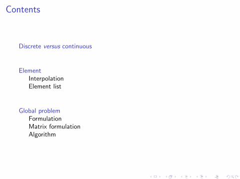
Continuous→ Discrete→Continuous
How much rain ?
Discrete versus continuous 3/67
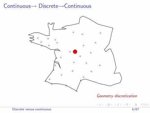
Continuous→ Discrete→Continuous
Geometry discretization
Discrete versus continuous 4/67
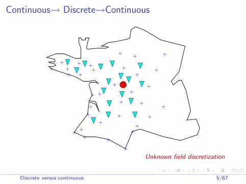
Continuous→ Discrete→Continuous
Unknown field discretization
Discrete versus continuous 5/67
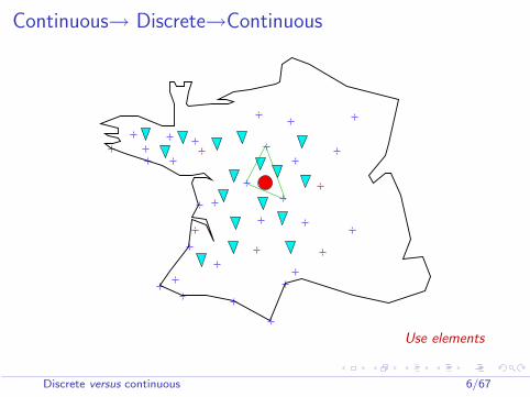
Continuous→ Discrete→Continuous
Use elements
Discrete versus continuous 6/67
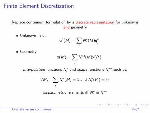
Finite Element Discretization
Replace continuum formulation by a discrete representation for unknownsand geometry
Unknown field:ue(M) =
∑i
Nei (M)qe
i
Geometry:
x(M) =∑
i
N∗ei (M)x(Pi )
Interpolation functions Nei and shape functions N∗ei such as:
∀M,∑
i
Nei (M) = 1 and Ne
i (Pj) = δij
Isoparametric elements iff Nei ≡ N∗ei
Discrete versus continuous 7/67
Contents
Discrete versus continuous
ElementInterpolationElement list
Global problemFormulationMatrix formulationAlgorithm
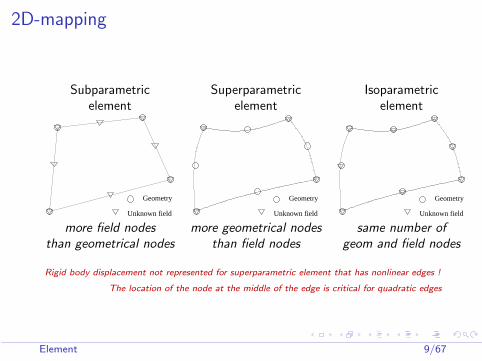
2D-mapping
Subparametric Superparametric Isoparametricelement element element
Geometry
Unknown field
Geometry
Unknown field
Geometry
Unknown field
more field nodes more geometrical nodes same number ofthan geometrical nodes than field nodes geom and field nodes
Rigid body displacement not represented for superparametric element that has nonlinear edges !
The location of the node at the middle of the edge is critical for quadratic edges
Element 9/67
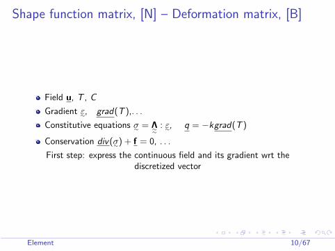
Shape function matrix, [N] – Deformation matrix, [B]
Field u, T , C
Gradient ε∼, grad(T ),. . .
Constitutive equations σ∼ = Λ∼∼: ε∼, q = −kgrad(T )
Conservation div(σ∼) + f = 0, . . .
First step: express the continuous field and its gradient wrt thediscretized vector
Element 10/67
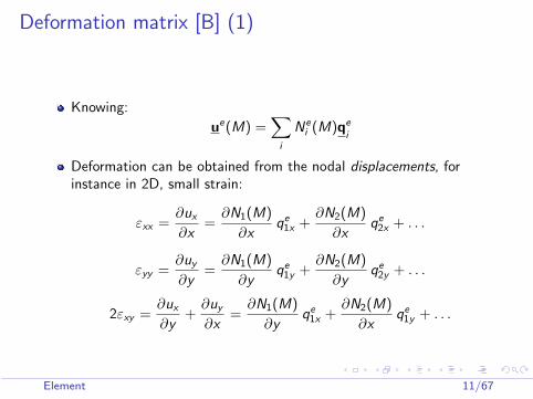
Deformation matrix [B] (1)
Knowing:
ue(M) =∑
i
Nei (M)qe
i
Deformation can be obtained from the nodal displacements, forinstance in 2D, small strain:
εxx =∂ux
∂x=
∂N1(M)
∂xqe
1x +∂N2(M)
∂xqe
2x + . . .
εyy =∂uy
∂y=
∂N1(M)
∂yqe
1y +∂N2(M)
∂yqe
2y + . . .
2εxy =∂ux
∂y+
∂uy
∂x=
∂N1(M)
∂yqe
1x +∂N2(M)
∂xqe
1y + . . .
Element 11/67
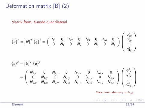
Deformation matrix [B] (2)
Matrix form, 4-node quadrilateral
ue = [N]T qe =
(N1 0 N2 0 N3 0 N4 00 N1 0 N2 0 N3 0 N4
)qe
1x
qe1y
...qe
4y
εe = [B]T qe
=
N1,x 0 N2,x 0 N3,x 0 N4,x 00 N1,y 0 N2,y 0 N3,y 0 N4,y
N1,y N1,x N2,y N2,x N3,y N3,x N4,y N4,x
qe1x
qe1y
...qe
4y
Shear term taken as γ = 2ε12
Element 12/67
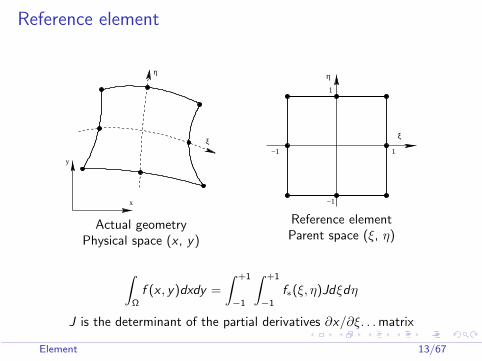
Reference element
x
y
ξ
η
Actual geometryPhysical space (x , y)
η
ξ
1
−1
−1 1
Reference elementParent space (ξ, η)
∫Ω
f (x , y)dxdy =
∫ +1
−1
∫ +1
−1
f∗(ξ, η)Jdξdη
J is the determinant of the partial derivatives ∂x/∂ξ. . . matrix
Element 13/67
Remarks on geometrical mapping
The values on an edge depends only on the nodal values on the sameedge (linear interpolation equal to zero on each side for 2-node lines,parabolic interpolation equal to zero for 3 points for 3-node lines)
Continuity...
The mid node is used to allow non linear geometries
Limits in the admissible mapping for avoiding singularities
Element 14/67
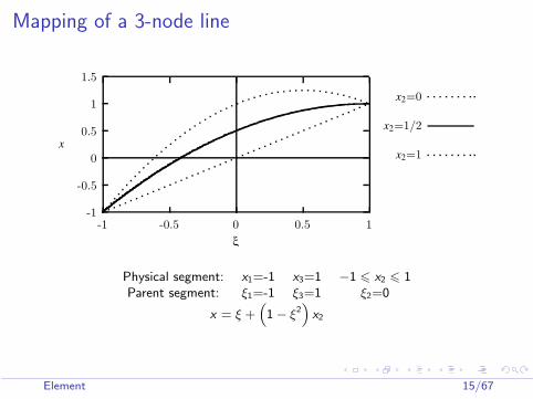
Mapping of a 3-node line
-1
-0.5
0
0.5
1
1.5
-1 -0.5 0 0.5 1
x
ξ
x2=0
x2=1/2
x2=1
Physical segment: x1=-1 x3=1 −1 6 x2 6 1Parent segment: ξ1=-1 ξ3=1 ξ2=0
x = ξ +“1− ξ2
”x2
Element 15/67
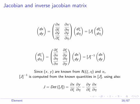
Jacobian and inverse jacobian matrix
(dxdy
)=
∂x
∂ξ
∂x
∂η∂y
∂ξ
∂y
∂η
(dξdη
)= [J]
(dξdη
)
(dξdη
)=
∂ξ
∂x
∂ξ
∂y∂η
∂x
∂η
∂y
(dxdy
)= [J]−1
(dxdy
)
Since (x , y) are known from Ni (ξ, η) and xi ,
[J]−1 is computed from the known quantities in [J], using also:
J = Det ([J]) =∂x
∂ξ
∂y
∂η− ∂y
∂ξ
∂x
∂η
Element 16/67
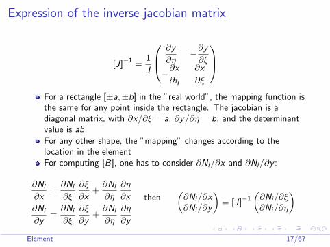
Expression of the inverse jacobian matrix
[J]−1 =1
J
∂y
∂η−∂y
∂ξ
−∂x
∂η
∂x
∂ξ
For a rectangle [±a,±b] in the ”real world”, the mapping function isthe same for any point inside the rectangle. The jacobian is adiagonal matrix, with ∂x/∂ξ = a, ∂y/∂η = b, and the determinantvalue is abFor any other shape, the ”mapping” changes according to thelocation in the elementFor computing [B], one has to consider ∂Ni/∂x and ∂Ni/∂y :
∂Ni
∂x=
∂Ni
∂ξ
∂ξ
∂x+
∂Ni
∂η
∂η
∂x
∂Ni
∂y=
∂Ni
∂ξ
∂ξ
∂y+
∂Ni
∂η
∂η
∂y
then(
∂Ni/∂x∂Ni/∂y
)= [J]−1
(∂Ni/∂ξ∂Ni/∂η
)
Element 17/67
Contents
Discrete versus continuous
ElementInterpolationElement list
Global problemFormulationMatrix formulationAlgorithm
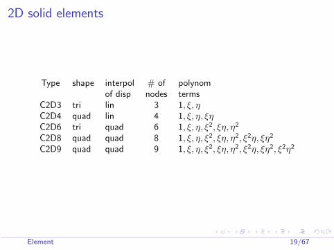
2D solid elements
Type shape interpol # of polynomof disp nodes terms
C2D3 tri lin 3 1, ξ, ηC2D4 quad lin 4 1, ξ, η, ξηC2D6 tri quad 6 1, ξ, η, ξ2, ξη, η2
C2D8 quad quad 8 1, ξ, η, ξ2, ξη, η2, ξ2η, ξη2
C2D9 quad quad 9 1, ξ, η, ξ2, ξη, η2, ξ2η, ξη2, ξ2η2
Element 19/67
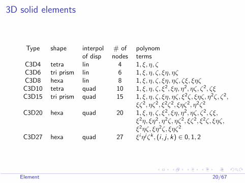
3D solid elements
Type shape interpol # of polynomof disp nodes terms
C3D4 tetra lin 4 1, ξ, η, ζC3D6 tri prism lin 6 1, ξ, η, ζ, ξη, ηζC3D8 hexa lin 8 1, ξ, η, ζ, ξη, ηζ, ζξ, ξηζC3D10 tetra quad 10 1, ξ, η, ζ, ξ2, ξη, η2, ηζ, ζ2, ζξC3D15 tri prism quad 15 1, ξ, η, ζ, ξη, ηζ, ξ2ζ, ξηζ, η2ζ, ζ2,
ξζ2, ηζ2, ξ2ζ2, ξηζ2, η2ζ2
C3D20 hexa quad 20 1, ξ, η, ζ, ξ2, ξη, η2, ηζ, ζ2, ζξ,ξ2η, ξη2, η2ζ, ηζ2, ξζ2, ξ2ζ, ξηζ,ξ2ηζ, ξη2ζ, ξηζ2
C3D27 hexa quad 27 ξiηjζk , (i , j , k) ∈ 0, 1, 2
Element 20/67
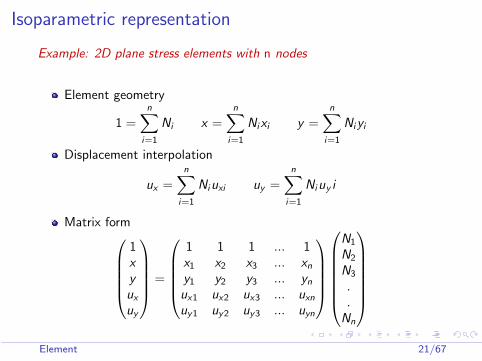
Isoparametric representation
Example: 2D plane stress elements with n nodes
Element geometry
1 =n∑
i=1
Ni x =n∑
i=1
Nixi y =n∑
i=1
Niyi
Displacement interpolation
ux =n∑
i=1
Niuxi uy =n∑
i=1
Niuy i
Matrix form1xyux
uy
=
1 1 1 ... 1x1 x2 x3 ... xn
y1 y2 y3 ... yn
ux1 ux2 ux3 ... uxn
uy1 uy2 uy3 ... uyn
N1
N2
N3
.
.Nn
Element 21/67
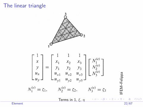
The linear triangle
IFEM
–Fel
ippa
Terms in 1, ξ, ηElement 22/67
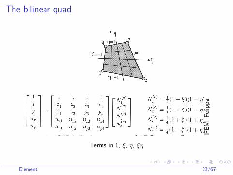
The bilinear quad
IFEM
–Fel
ippa
Terms in 1, ξ, η, ξη
Element 23/67
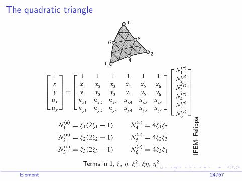
The quadratic triangle
IFEM
–Fel
ippa
Terms in 1, ξ, η, ξ2, ξη, η2
Element 24/67
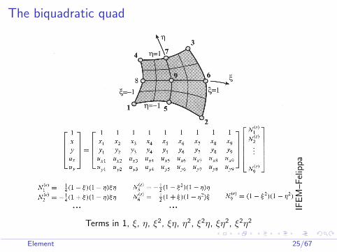
The biquadratic quad
IFEM
–Fel
ippa
Terms in 1, ξ, η, ξ2, ξη, η2, ξ2η, ξη2, ξ2η2
Element 25/67
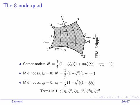
The 8-node quad
IFEM
–Fel
ippa
Corner nodes: Ni =1
4(1 + ξξi )(1 + ηηi )(ξξi + ηηi − 1)
Mid nodes, ξi = 0: Ni =1
2(1− ξ2)(1 + ηηi )
Mid nodes, ηi = 0: nI =1
2(1− η2)(1 + ξξi )
Terms in 1, ξ, η, ξ2, ξη, η2, ξ2η, ξη2
Element 26/67
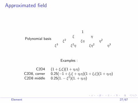
Approximated field
Polynomial basis
1ξ η
ξ2 ξη η2
ξ3 ξ2η ξη2 η3
Examples :
C2D4 (1 + ξiξ)(1 + ηiη)C2D8, corner 0.25(−1 + ξiξ + ηiη)(1 + ξiξ)(1 + ηiη)C2D8 middle 0.25(1.− ξ2)(1. + ηiη)
Element 27/67
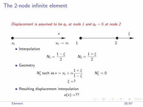
The 2-node infinite element
Displacement is assumed to be q1 at node 1 and q2 = 0 at node 2
x ξ
x1 x2 →∞ 1 2
Interpolation
N1 =1− ξ
2N2 =
1 + ξ
2
Geometry
N∗1 such as x = x1 + α1 + ξ
1− ξN∗2 = 0
ξ =?
Resulting displacement interpolation
u(x) =??
Element 28/67
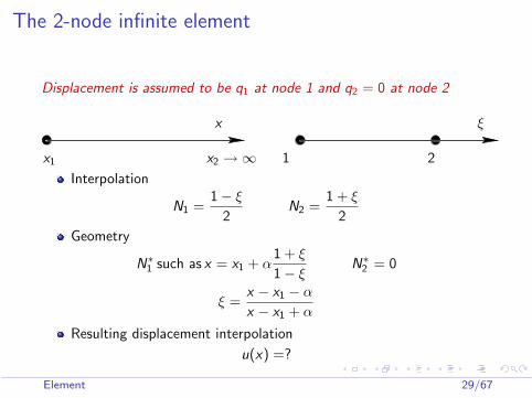
The 2-node infinite element
Displacement is assumed to be q1 at node 1 and q2 = 0 at node 2
x ξ
x1 x2 →∞ 1 2
Interpolation
N1 =1− ξ
2N2 =
1 + ξ
2
Geometry
N∗1 such as x = x1 + α1 + ξ
1− ξN∗2 = 0
ξ =x − x1 − α
x − x1 + α
Resulting displacement interpolation
u(x) =?
Element 29/67
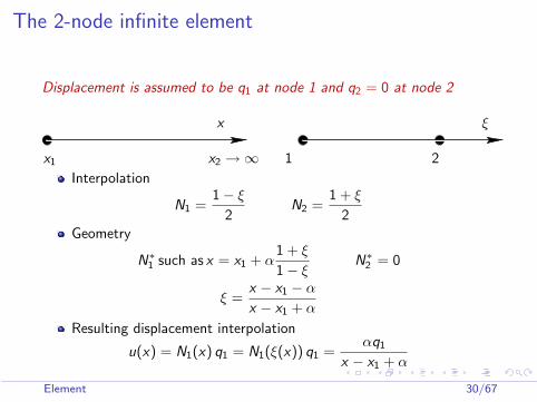
The 2-node infinite element
Displacement is assumed to be q1 at node 1 and q2 = 0 at node 2
x ξ
x1 x2 →∞ 1 2
Interpolation
N1 =1− ξ
2N2 =
1 + ξ
2Geometry
N∗1 such as x = x1 + α1 + ξ
1− ξN∗2 = 0
ξ =x − x1 − α
x − x1 + α
Resulting displacement interpolation
u(x) = N1(x) q1 = N1(ξ(x)) q1 =αq1
x − x1 + α
Element 30/67
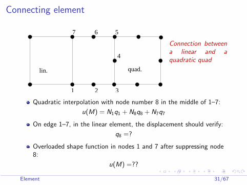
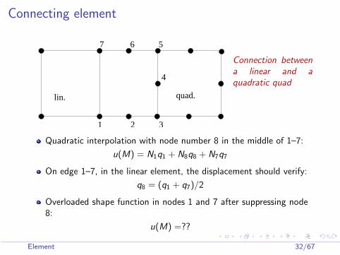
Connecting element
1 2 3
7 6 5
4
lin. quad.
Connection betweena linear and aquadratic quad
Quadratic interpolation with node number 8 in the middle of 1–7:
u(M) = N1q1 + N8q8 + N7q7
On edge 1–7, in the linear element, the displacement should verify:
q8 =?
Overloaded shape function in nodes 1 and 7 after suppressing node8:
u(M) =??
Element 31/67
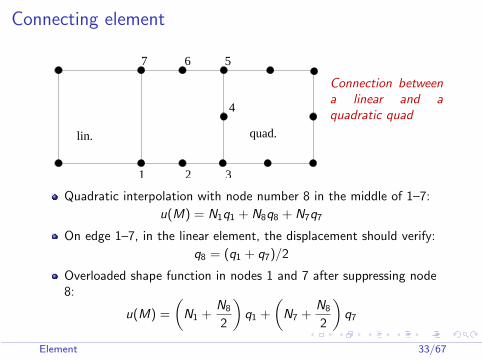
Connecting element
1 2 3
7 6 5
4
lin. quad.
Connection betweena linear and aquadratic quad
Quadratic interpolation with node number 8 in the middle of 1–7:
u(M) = N1q1 + N8q8 + N7q7
On edge 1–7, in the linear element, the displacement should verify:
q8 = (q1 + q7)/2
Overloaded shape function in nodes 1 and 7 after suppressing node8:
u(M) =??
Element 32/67
Connecting element
1 2 3
7 6 5
4
lin. quad.
Connection betweena linear and aquadratic quad
Quadratic interpolation with node number 8 in the middle of 1–7:
u(M) = N1q1 + N8q8 + N7q7
On edge 1–7, in the linear element, the displacement should verify:
q8 = (q1 + q7)/2
Overloaded shape function in nodes 1 and 7 after suppressing node8:
u(M) =
(N1 +
N8
2
)q1 +
(N7 +
N8
2
)q7
Element 33/67
Contents
Discrete versus continuous
ElementInterpolationElement list
Global problemFormulationMatrix formulationAlgorithm
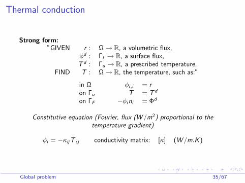
Thermal conduction
Strong form:”GIVEN r : Ω → R, a volumetric flux,
φd : Γf → R, a surface flux,T d : Γu → R, a prescribed temperature,
FIND T : Ω → R, the temperature, such as:”
in Ω φi,i = ron Γu T = T d
on ΓF −φini = Φd
Constitutive equation (Fourier, flux (W /m2) proportional to thetemperature gradient)
φi = −κijT ,j conductivity matrix: [κ] (W /m.K )
Global problem 35/67
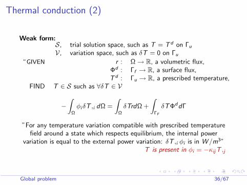
Thermal conduction (2)
Weak form:S, trial solution space, such as T = T d on Γu
V, variation space, such as δT = 0 on Γu
”GIVEN r : Ω → R, a volumetric flux,Φd : Γf → R, a surface flux,T d : Γu → R, a prescribed temperature,
FIND T ∈ S such as ∀δT ∈ V
−∫
Ω
φiδT ,i dΩ =
∫Ω
δTrdΩ +
∫ΓF
δTΦddΓ
”For any temperature variation compatible with prescribed temperaturefield around a state which respects equilibrium, the internal power
variation is equal to the external power variation: δT ,i φi is in W /m3”T is present in φi = −κijT ,j
Global problem 36/67
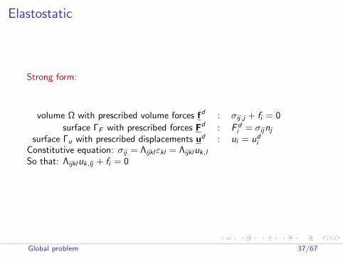
Elastostatic
Strong form:
volume Ω with prescribed volume forces fd : σij,j + fi = 0
surface ΓF with prescribed forces Fd : F di = σijnj
surface Γu with prescribed displacements ud : ui = udi
Constitutive equation: σij = Λijklεkl = Λijkluk,l
So that: Λijkluk,lj + fi = 0
Global problem 37/67
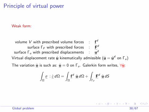
Principle of virtual power
Weak form:
volume V with prescribed volume forces : fd
surface ΓF with prescribed forces : Fd
surface Γu with prescribed displacements : ud
Virtual displacement rate u kinematically admissible (u = ud on Γu)
The variation u is such as: u = 0 on Γu. Galerkin form writes, ∀u:∫Ω
σ∼ : ε∼dΩ =
∫Ω
fd u dΩ +
∫ΓF
Fd u dS
Global problem 38/67
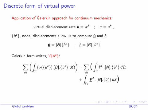
Discrete form of virtual power
Application of Galerkin approach for continuum mechanics:
virtual displacement rate u ≡ wh ; σ∼ ≡ uh,x
ue, nodal displacements allow us to compute u and ε∼:
u = [N]ue ; ε∼ = [B]ue
Galerkin form writes, ∀ue:∑elt
(∫Ω
σ(ue).[B].ue dΩ
)=∑elt
(∫
Ω
fd .[N].ue dΩ
+
∫ΓF
Fd .[N].ue dS)
Global problem 39/67
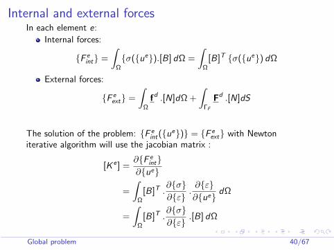
Internal and external forcesIn each element e:
Internal forces:
F eint =
∫Ω
σ(ue).[B] dΩ =
∫Ω
[B]T σ(ue) dΩ
External forces:
F eext =
∫Ω
fd .[N]dΩ +
∫ΓF
Fd .[N]dS
The solution of the problem: F eint(ue) = F e
ext with Newtoniterative algorithm will use the jacobian matrix :
[K e ] =∂F e
int∂ue
=
∫Ω
[B]T .∂σ∂ε
.∂ε∂ue
dΩ
=
∫Ω
[B]T .∂σ∂ε
.[B] dΩ
Global problem 40/67
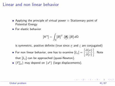
Linear and non linear behavior
Applying the principle of virtual power ≡ Stationnary point ofPotential Energy
For elastic behavior
[K e ] =
∫Ω
[B]T .[Λ∼∼] .[B] dΩ
is symmetric, positive definite (true since σ∼ and ε∼ are conjugated)
For non linear behavior, one has to examine [Lc ] =
[∂σ∂ε
]. Note
that [Lc ] can be approached (quasi-Newton).
F eext may depend on ue (large displacements).
Global problem 41/67
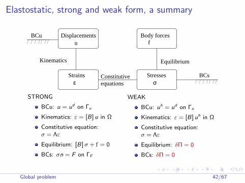
Elastostatic, strong and weak form, a summary
Displacementsu
Body forces f
Strains Stressesε σ
BCu
BCs
Kinematics
Constitutiveequations
Equilibrium
STRONG
BCu: u = ud on Γu
Kinematics: ε = [B] u in Ω
Constitutive equation:σ = Λε
Equilibrium: [B] σ + f = 0
BCs: σn = F on ΓF
WEAK
BCu: uh = ud on Γu
Kinematics: ε = [B] uh in Ω
Constitutive equation:σ = Λε
Equilibrium: δΠ = 0
BCs: δΠ = 0
Global problem 42/67
Contents
Discrete versus continuous
ElementInterpolationElement list
Global problemFormulationMatrix formulationAlgorithm
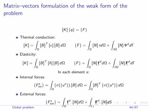
Matrix–vectors formulation of the weak form of theproblem
[K ] q = F
Thermal conduction:
[K ] =
∫Ω
[B]T [κ] [B] dΩ F =
∫Ω
[N] rdΩ +
∫∂Ω
[N] ΦddΓ
Elasticity:
[K ] =
∫Ω
[B]T [Λ] [B] dΩ F =
∫Ω
[N] fddΩ +
∫∂Ω
[N]FddΓ
In each element e:Internal forces:
F eint =
∫Ω
σ(ue).[B] dΩ =
∫Ω
[B]T σ(ue) dΩ
External forces:
F eext =
∫Ω
fd .[N]dΩ +
∫ΓF
Fd .[N]dSGlobal problem 44/67
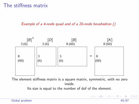
The stiffness matrix
Example of a 4-node quad and of a 20-node hexahedron ()
[B]T [D] [B] [K ]
=
3 (6) 3 (6) 8 (60) 8 (60)
8 3 3 8(60) (6) (6) (60)
The element stiffness matrix is a square matrix, symmetric, with no zeroinside.
Its size is equal to the number of dof of the element.
Global problem 45/67
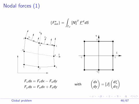
Nodal forces (1)
F eext =
∫ΓF
[N]T F ddS
Fn
1
5
7F t
8
4
23
6
ξ
η
η
ξ
1
−1
−1 1
Fxds = Ftdx − Fndy
Fyds = Fndx + Ftdywith
(dxdy
)= [J]
(dξdη
)
Global problem 46/67
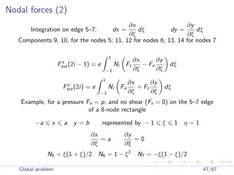
Nodal forces (2)
Integration on edge 5–7: dx =∂x
∂ξdξ dy =
∂y
∂ξdξ
Components 9, 10, for the nodes 5; 11, 12 for nodes 6; 13, 14 for nodes 7
F eext(2i − 1) = e
∫ 1
−1
Ni
(Ft
∂x
∂ξ− Fn
∂y
∂ξ
)dξ
F eext(2i) = e
∫ 1
−1
Ni
(Fn
∂x
∂ξ+ Ft
∂y
∂ξ
)dξ
Example, for a pressure Fn = p, and no shear (Ft = 0) on the 5–7 edgeof a 8-node rectangle
−a 6 x 6 a y = b represented by − 1 6 ξ 6 1 η = 1
∂x
∂ξ= a
∂y
∂ξ= 0
N5 = ξ(1 + ξ)/2 N6 = 1− ξ2 N7 = −ξ(1− ξ)/2
Global problem 47/67
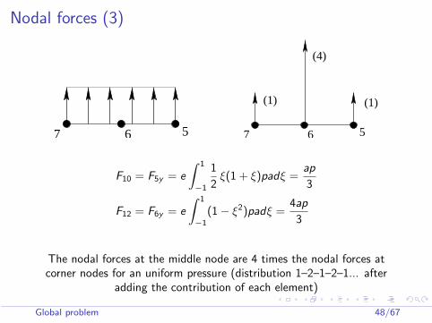
Nodal forces (3)
7 6 5 7 6 5
(1)
(4)
(1)
F10 = F5y = e
∫ 1
−1
1
2ξ(1 + ξ)padξ =
ap
3
F12 = F6y = e
∫ 1
−1
(1− ξ2)padξ =4ap
3
The nodal forces at the middle node are 4 times the nodal forces atcorner nodes for an uniform pressure (distribution 1–2–1–2–1... after
adding the contribution of each element)
Global problem 48/67
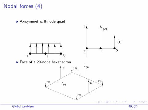
Nodal forces (4)
Axisymmetric 8-node quad
7 6 57 6 5
(2)
(1)
z
Face of a 20-node hexahedron
(4)
(4)
(4)
(4)
(−1)
(−1)
(−1)
(−1)
Global problem 49/67
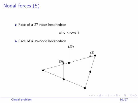
Nodal forces (5)
Face of a 27-node hexahedron
who knows ?
Face of a 15-node hexahedron
(3)
(3)
(3)
Global problem 50/67
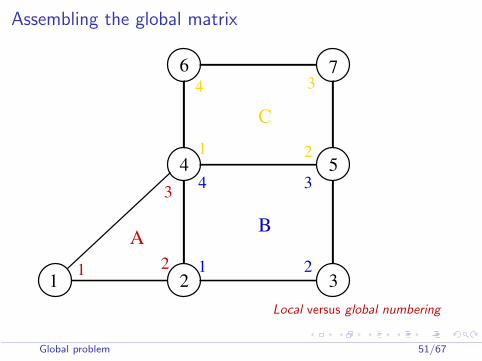
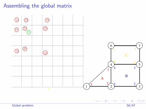
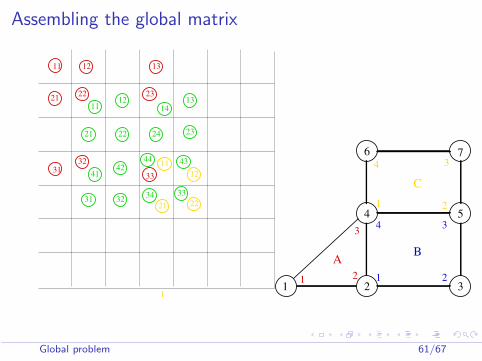
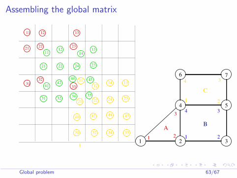
Assembling the global matrix
2 3
4 5
7
1
6
AB
1 1
1
2 2
3 3
3
4
4
C
2
Local versus global numbering
Global problem 51/67
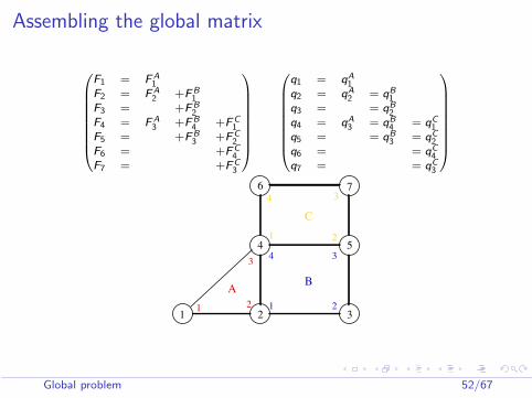
Assembling the global matrix
0BBBBBBBB@
F1 = FA1
F2 = FA2 +FB
1F3 = +FB
2F4 = FA
3 +FB4 +FC
1F5 = +FB
3 +FC2
F6 = +FC4
F7 = +FC3
1CCCCCCCCA
0BBBBBBBB@
q1 = qA1
q2 = qA2 = qB
1q3 = = qB
2q4 = qA
3 = qB4 = qC
1q5 = = qB
3 = qC2
q6 = = qC4
q7 = = qC3
1CCCCCCCCA
2 3
4 5
7
1
6
AB
1 1
1
2 2
3 3
3
4
4
C
2
Global problem 52/67
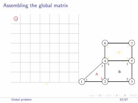
Assembling the global matrix
11
12 3
4 5
7
1
6
AB
1 1
1
2 2
3 3
3
4
4
C
2
Global problem 53/67
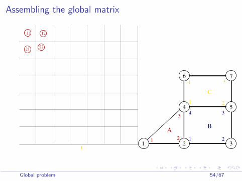
Assembling the global matrix
21
11 12
22
12 3
4 5
7
1
6
AB
1 1
1
2 2
3 3
3
4
4
C
2
Global problem 54/67
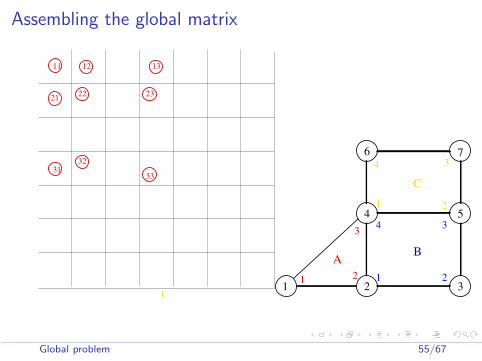
Assembling the global matrix
21
11 12 13
22 23
3231
33
12 3
4 5
7
1
6
AB
1 1
1
2 2
3 3
3
4
4
C
2
Global problem 55/67
Assembling the global matrix
21
11 12 13
1122 23
3231
33
12 3
4 5
7
1
6
AB
1 1
1
2 2
3 3
3
4
4
C
2
Global problem 56/67

Assembling the global matrix
21
11 12 13
1122 23
3231
33
12 3
4 5
7
1
6
AB
1 1
1
2 2
3 3
3
4
4
C
2
Global problem 57/67
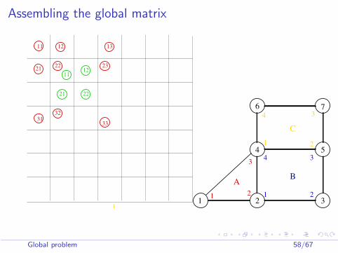
Assembling the global matrix
21
11 12 13
1122
1223
2221
3231
33
12 3
4 5
7
1
6
AB
1 1
1
2 2
3 3
3
4
4
C
2
Global problem 58/67
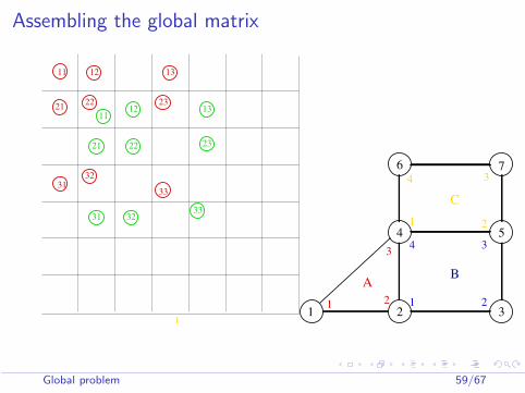
Assembling the global matrix
33
21
11 12 13
1122
1223
13
232221
3231
31 32
33
12 3
4 5
7
1
6
AB
1 1
1
2 2
3 3
3
4
4
C
2
Global problem 59/67

Assembling the global matrix
44
33
1133
43
34
21
11 12 13
1122
1214
2313
23242221
4132
31
31 32
42
12 3
4 5
7
1
6
AB
1 1
1
2 2
3 3
3
4
4
C
2
Global problem 60/67
Assembling the global matrix
44
33
1133
22
12
21
43
34
21
11 12 13
1122
1214
2313
23242221
4132
31
31 32
42
12 3
4 5
7
1
6
AB
1 1
1
2 2
3 3
3
4
4
C
2
Global problem 61/67

Assembling the global matrix
44
33
1133
22
12
21
43
34 23
13
31
21
11 12 13
1122
1214
2313
23242221
4132
31
31 32
42
32 33
12 3
4 5
7
1
6
AB
1 1
1
2 2
3 3
3
4
4
C
2
Global problem 62/67
Assembling the global matrix
44
33
1133
22
12
21
43
34 23
13
31
21
11 12 13
1122
1214
2313
23242221
4132
31
31 32
42 14
43444241
3432 33
24
12 3
4 5
7
1
6
AB
1 1
1
2 2
3 3
3
4
4
C
2
Global problem 63/67
Contents
Discrete versus continuous
ElementInterpolationElement list
Global problemFormulationMatrix formulationAlgorithm
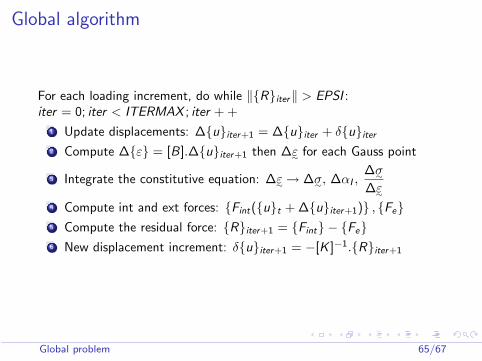
Global algorithm
For each loading increment, do while ‖Riter‖ > EPSI :iter = 0; iter < ITERMAX ; iter + +
1 Update displacements: ∆uiter+1 = ∆uiter + δuiter
2 Compute ∆ε = [B].∆uiter+1 then ∆ε∼ for each Gauss point
3 Integrate the constitutive equation: ∆ε∼→ ∆σ∼, ∆αI ,∆σ∼∆ε∼
4 Compute int and ext forces: Fint(ut + ∆uiter+1) , Fe5 Compute the residual force: Riter+1 = Fint − Fe6 New displacement increment: δuiter+1 = −[K ]−1.Riter+1
Global problem 65/67
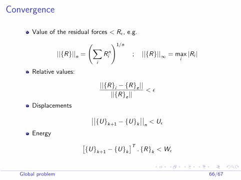
Convergence
Value of the residual forces < Rε, e.g.
||R||n =
(∑i
Rni
)1/n
; ||R||∞ = maxi|Ri |
Relative values:
||Ri − Re ||||Re ||
< ε
Displacements ∣∣∣∣Uk+1 − Uk
∣∣∣∣n
< Uε
Energy [Uk+1 − Uk
]T. Rk < Wε
Global problem 66/67


![Finite [Mayjune2013]](https://img.pdfslide.tips/doc/110x75/55cf8d2c5503462b1392af25/finite-mayjune2013.jpg)