Fiscal policy and economic growth - 國立臺灣大學homepage.ntu.edu.tw/~kslin/macro2009/Easterly and Rebelo 1993JME.pdf · 418 W. Easterly and S. Rebelo, Fiscal policy and economic

Journal of Monetary Economics 32 (1993) 417-458. North-Holland

Fiscal policy and economic growth

An empirical investigation*

William Easterly World Bank, Washington, DC 20433, USA

Sergio Rebelo+ University of Rochester. Rochester, NY 14627, USA

Received March 1993, final version received September 1993

This paper describes the empirical regularities relating fiscal policy variables, the level of development, and the rate of growth. We employ historical data, recent cross-section data, and newly constructed public investment series. Our main findings are: (i) there is a strong association between the develop ment level and the fiscal structure: poor countries rely heavily on international trade taxes, while income taxes are only important in developed economies; (ii) fiscal policy is influenced by the scale of the economy, measured by its population; (iii) investment in transport and communication is consistently correlated with growth; (iv) the effects of taxation are difficult to isolate empirically.

Key words: Growth; Development; Fiscal policy

JEL classification: 040; E62

1. Introduction

If you ask an economist to explain the growth performance of a particular country he is likely to mention fiscal policy as being an important growth

Correspondence to: Sergio Rebelo, Department of Economics, University of Rochester, Rochester, NY 14627, USA.

*We wish to thank George Clarke, Rui Albuquerque, and Piyabha Kongsamut for their dedicated research assistance. We benefited from the comments of Robert Barro, Oded Galor, Robert King, Larry Kotlikoff, Ross Levine, Charles Plosser, Jonathan Skinner, Nicholas Stern, Nancy Stokey, Guido Tabellini, and Vito Tanzi. We also benefited from feedback provided by seminar participants at Boston College, Brown, Georgetown, Harvard, MIT, Northwestern, NYU, Pennsylvania, Vir- ginia, and UCLA, and by participants at the Conferences on Economic Growth in Estoril, Portugal, in January 1993, and at the World Bank, in February 1993. The usual disclaimer applies.

‘Also affiliated with the Portuguese Catholic University, Lisbon, the Bank of Portugal, Lisbon, and the NBER, Cambridge, Massachusetts.

0304-3932/93/$06.00 0 1993-Elsevier Science Publishers B.V. All rights reserved

418 W. Easterly and S. Rebelo, Fiscal policy and economic growth

determinant. This deep-seeded belief that taxation, public investment, and other aspects of fiscal policy can contribute to growth miracles as well as to enduring stagnation has been articulated in the context of growth models during the past three decades.

Growth models, both old and new, feature simple channels that link certain taxes to the rate of growth. Increases in income taxes, for example, lower the net rate of return to private investment, making investment activities less attractive and lowering the rate of growth. It is hard to think of an influence on the private real rate of return and on the growth rate that is more direct than that of income taxes. If these do not affect the rate of growth, what does?

Unfortunately, the empirical evidence that is currently available to shed light of the importance of fiscal policy in determining growth is sparse.’ This sparseness reflects the difficulties involved in measuring the variables that theory predicts to be important growth determinants: marginal tax rates and subsidies, and levels of public investment.

Our goal in this paper is to provide a comprehensive summary of the statistical association between measures of fiscal policy, the level of development, and the rate of growth using standard data sources combined with newly created data for public investment. We will document the empirical regularities that emerge in a broad cross-section of countries with data for the period 1970 to 1988 as well those associated with the long-run historical data that is available for a small set of countries. There is substantial measurement error in both of these data sets, but there is also information.

The next section of the paper reviews briefly the theoretical literature on fiscal policy and growth. Our empirical investigation starts in section 3 which uses fiscal data for the period 1970-1988 in the context of cross-section regressions made popular by the work of Barro (1991). We find that the high correlation between many fiscal variables and the level of income in the beginning of the period makes it difficult to isolate the effect of fiscal policy in the context of the Barro regression. This correlation with initial income leads us to study in section 4 whether fiscal policy is endogenous in’the sense of being related to characteristics such as the level of development and the overall scale of the economy.

Our empirical findings are summarized by the following list of ten stylized facts. We use the term ‘cross-section’ to refer to our cross-section data set of about 100 countries for the period 1970-1988. The term ‘historical data’ refers to our panel of annual data for 28 countries comprising the period from 1870 to 1988.

‘Prior empirical analyses of the relation between fiscal policy and growth include Garcia-Mila (1987), Crier and Tullock (1989), Koester and Kormendi (1989), Plosser (1992), and Engen and Skinner (1992).

W. Easterly and S. Rebeio, Fiscal pohcy and economic growth 419

(1) The share of public investment in transport and communication is robustly correlated with growth in our cross-section when we control for the slew of variables standard in cross-section studies. This partial correlation survives when we instrument for this variable (although the resulting coefficient is implausibly high).

(2) The government’s budget surplus is also consistently correlated with growth and private investment in our cross-section.

(3) The link between most other fiscal variables and growth is statistically fragile. The statistical sig~i~cance of these variables in a cross-section regression context depends heavily on what other control variables are included in the regression. This fragility is partly a result of multicollinear- ity. Fiscal variables tend to be highly correlated with the level of income in the beginning of the period and are highly correlated among themselves (countries that have higher taxes also have higher spending).

(4) Government revenue/GDP rises with per capita income (Wagner’s Law) in both the cross-section and the historical data sets.

(5) In both of our data sets, we observe that as income rises, international trade taxes fall as a share of government revenue, while the share of income taxes rises.

(6) In our cross-section higher income countries have relatively higher government health expenditures and larger social security programs.

(7) The choice of fiscal instruments seems to be related to the scale of the economy. In both of our data sets we find that as population increases the share of trade taxes in revenue falls and the share of income taxes rises. This relation continues to hold if we control for income and for the trade share.

(8) Our cross-section data shows that high population countries spend more on defense and less on transport and communication.

(9) High levels of inequality in income distribution, observed prior to 1970, were associated with higher levels of publicly provided education in the period from 1970 to 1988.

(10) There are no significant differences in the fiscal policies adopted by democracies and nondemo~racies once we control for the level of income.

2. The theoretical predictions

The development of the neoclassical model provided public finance students with a theoretical construct suitable to think about the growth effects of fiscal policy. Researchers such as Sato (1967), Krzyzaniak (1967), and Feldstein (1974) used versions of the Solow (1956) model to study the dynamic impact of taxation. More recently, Charnley (1986) and Judd (1985) among others, have used the neoclassical growth model with an endogenous savings rate developed by Cass (1965) and Koopmans (1965) as a laboratory to study fiscal policy.


Diamond’s (1965) overlapping generations version of the neoclassical model has also been extensively used - by Summers (198 l), Auerbach and Kotlikoff (1987), and others - to examine the dynamic effects of fiscai policy.

Since in the neoclassical model steady state growth is driven by exogenous factors - the dynamics of population and of technological progress - fiscal policy can only affect the rate of growth during the transition to the steady state. Because of this fact, the conventional wisdom based on the neoclassical model has been that differences in tax systems and in debt and expenditure policy can be impo~ant determinants of the level of output but are unlikely to have an important effect on the rate of growth.‘-

This conventional wisdom contrasts with the predictions of Eaton’s (1981) stochastic growth model, which features a linear production function, as well as with those of more recent ‘endogenous growth’ models [e.g., a version of Romer’s (1986) model that admits steady state growth, the economies with convex technologies explored by Jones and Manueili (1990) and Rebel0 (1991), and the ‘lab-equipment model’ of Rivera-Batiz and Romer (199lf-J. In these models fiscal policy can be one of the main determinants of the observed differences in growth experiences.

‘Endogenous growth’ models tend to transform the temporary growth effects of fiscal policy implied by the neoclassical model into permanent growth effects. The strength of these effects varies, however, from model to model, depending heavily on the elasticity of labor supply and on aspects of the technology to accumulate human capital and to create new goods about which very little is currently known [see Jones, Manuelli, and Rossi (1993) and Stokey and Rebel0 (199311.

In order to isolate the effect of each fiscal instrument it is standard in public finance to assume that the impact of a change in a fiscal variable on government revenue or expenditure is compensated with lump sum taxes or subsidies. We describe below the long-run effect of permanent changes in various fiscal instruments under this assumption.

Most growth models predict that taxes on investment and income have a detrimental effect on growth. These taxes affect the rate of growth through a simple, direct, channel: they reduce the private returns to accumulation. But not all taxes affect the rate of growth. In models with exogenous labor supply the growth rate is immune to the level of consumption taxes; these taxes do not distort the relative price of consumption today versus tomorrow, leaving unaffected the incentive to accumulate capital.

The effect of an increase in government consumption should also be nil if we view this component of public expenditures as leaving the productivity of the

‘In the standard neoclassical model with a conventional value for the share of capital in output the transitional dynamics can only be important if the real interest rate takes on implausibly high values [King and Rebel0 (1993)].

W. Easterly and S. Rebelo. Fiscal policy and economic growth 421

private sector unaffected. In contrast, the effect of public investment should be positive since this type of activity is likely to enhance the productivity of the private sector [Aschauer (1989) Barro (199011.

When we change more than one instrument at a time we get a combination of these various partial effects, For example, the effects of an increase in government investment financed by income taxes is ambiguous [see Barro (1990)].

The effects of government deficits are more complex. In overlapping generations models government deficits tend to reduce the savings rate and the rate of growth [see Alogoskoufis and Ploeg (1991)]. In infinite horizon models the effects of deficits depend on the variables that have to be adjusted in the future to compensate for the deficits. If a higher deficit today will later be compensated by higher consumption or income taxes the rate of growth will decline.

In the empirical analysis that we describe in the next section we pay particular attention to two of the strongest predictions of growth models: that high income taxes lower the rate of growth and that high public spending on infrastructure investment raises growth.

3. Recent cross-section evidence

Our cross-section data set comprises the period 1970-1988 and combines information from five sources: Summers and Heston (1991) Barro and Wolf (1989) the Government Financial Statistics (GFS), the International Financial Statistics (IFS), and Easterly, Rodriguez, and Schmidt-Hebbel (1993). Later on in this section we also explore new data for public investment that we created using information contained in World Bank reports.

GFS, which is our main source of fiscal data suffers from two relevant shortcomings: (i) it includes only Central government activities and thus excludes local governments and public enterprises (although it includes transfers from the Central government to both local governments and public enterprises), and (ii) for some years and some countries the GFS statistics are based on budget data.

A complete list of the fiscal variables that we employed, as well as their sample means and standard deviations, is included in the appendix. Unless we state otherwise all fiscal variables are expressed as percentages of GDP and correspond to averages over the 1970-1988 period. We will explore mainly the cross-section dimension of the data because Easterly, Kremer, Pritchett, and Summers (1993) show that the variability over time of country characteristics adds little explanatory power.

3.1. Measuring marginal tax rates

The most important obstacle to an empirical investigation of the effects of fiscal policy on growth is that marginal tax rates and subsidies - which are the

422 W. Easterly and S. Rebelo. Fiscal policy and economic growth

relevant variables according to theory - are not observable. To compute marginal income tax rates one would ideally use the methodology of Barro and Sahasakul(l983). However, this requires information on individual incomes and taxes that is currently publicly available only for a small set of developed countries. We have explored four approaches to measuring tax rates, each with its own problems.3

Statutory tax rates on income are available for a cross-section of developing countries [see Sicat and Virmani (1988)]. We included these tax rates in our data set, but given that tax evasion is an important phenomenon in LDC’s, we suspect that these rates grossly overestimate the distortions associated with income taxation. Colombia is a representative example of tax evasion. Its personal income tax in 1984 allowed for very few deductions and credits and featured marginal tax rates that ranged between 7% and 49%. Yet, the revenue collected in 1984 represented only 1.75% of personal income.

We use the revenue from different types of taxes expressed as a fraction of GDP as a measure of the tax distortions. In the case of the income tax this would only correspond to the marginal tax rate on income if the tax were proportional. Even stronger assumptions are needed to guarantee that the fraction of revenue in GDP corresponds to marginal tax rates in the case of taxes on investment and on consumption. For this reason, we also constructed tax rates as the ratio of a specific type of revenue to the corresponding tax base (e.g., trade tax revenue/total trade or personal income tax/personal income).

We used the income-weighted marginal income tax rates computed in Easterly and Rebel0 (1993) where we employ a method that combines information on the lowest and the highest statutory tax rates, on the level of income for which taxes are zero, on the distribution of income, and on the income tax revenue collected.

Finally, we computed ‘marginal’ taxes rates by regressing the revenue from each type of tax on its tax base, as in Koester and Kormendi (1989). Unfortu- nately, the results of some of these regressions tend to vary significantly with the sample period employed since a significant number of LDCs reformed their tax system during the 1980~.~ This instability is also problematic for our ratios of revenue to the tax base or to GDP.

While the statutory tax rates tend to overestimate the distortion effects of taxation, the three types of measures discussed above tend to underestimate

3We also explored the possibility of computing statutory effective marginal tax rates on capital income along the lines of King and Fullerton (1984), taking advantage of the software developed by Dunn and Pellechio (1990) which can produce effective marginal tax rates for various developing countries. We found, as is common in this literature, that the effective marginal tax rates were very sensitive to the mix of assets involved in the project as well as to the choice of financing arrangements.

4Countries for which the regression coefficients are unstable generally have negative slope coefficients. We discarded those countries from our sample and retained only the ones with positive ‘marginal’ tax rates.

W. Easterly and S. Rebelo, Fiscal policy and economic growth 423

Table 1

Simple correlations of fiscal variables with per capita growth rate, 1970-88.

Averages 1970-88

Central government surplus/GDP 0.36 Consolidated public surplus/GDP 0.36

Revenue components as shares of GDP: Total revenue including grants Total revenue Tax revenue Nontax revenue Current revenue Social security contributions

0.22 0.27 0.20 0.34 0.27 0.18

Expenditure components as shares of GDP: Government consumption [Barre-Wolf (1989)] Government consumption excluding defense and education [Barro-Wolf (1989)] General public services Expenditures on social security Government transfers [Barro-Wolf (398931

- 0.28 - 0.32 - 0.30

0.19 0.23

Other tax variables: ‘Marginal’ income tax rate from regression of income tax revenue on GDP - 0.26 Standard deviation of ratio of domestic taxes to consumption plus investment - 0.39 Standard deviation of ratio of international trade taxes to imports plus exports - 0.18

those distortion effects. The key piece of information used in constructing those three measures is the revenue collected by the government. Taxes that generate little revenue are implicitly assumed to create small distortions. In practice, however, there are highly distortionary taxes that generate little revenue (the corporate income tax in the U.S., whose revenue is currently 2% of GNP, is often thought to be one such example).

3.2. Cross-section regressions

Table 1 reports the simple correlations between fiscal variables and the growth rate that are statistically significant. Existing theoretical models make no predictions about the sign of unconditional correlations. However, we will later show that the government surplus, government consumption, and the ‘marginal’ tax rate on income (computed with a time-series regression) continue to be correlated with growth after we control for the effects of other variables.

Our point of departure for a multivariate analysis is a version of the Barro (1991) regression. We followed Levine and Renelt (1992) in using World Bank data instead of Summers and Heston (1991) data to construct per capita income growth rates. This procedure reduces the possibility of the negative coefficient on initial income, typically found in Barro (1991) type regressions, being an

IMa- c


artifact of measurement error in income. Watson’s (1992) finding that the least squares growth rate is more robust to differences in the serial correlation proper- ties of the data than the geometric rate of growth led us to compute all growth rates by running a least squares regression of the logarithm of income on time.

Our basic regression, with t-statistics given in parentheses, is the following:’

GROWTH RATE OF PER CAPITA GDP 1970-88

= 0.003 - 0.004 (PER CAPITA GDP 1960)

(0.51) ( - 2.81)

+ 0.023 (PRIMARY ENROLLMENT 1960)

(3.15)

+ 0.025 (SECONDARY ENROLLMENT 1960) (1.88)

- 0.003 (ASSASSINATIONS PER MILLION) ( - 1.47)

- 0.01 (REVOLUTIONS AND COUPS)

( - 1.29)

- 1.157 (WAR CASUALTIES PER CAPITA).

( - 1.67)

The R2 of this regression is 0.29, while the number of observations employed is 105.

In extensions of the neoclassical growth model such as Mankiw, Romer, and Weil (1992) and in endogenous growth models such as Lucas (1988) the rate of growth is a function of two state variables: the initial level of physical capital and the initial level of human capital. In models such as those of Becker, Murphy, and Tamura (1990) and Azariadis and Drazen (1990) the initial level of human capital is also an important determinant of future growth. The two school enrollment variables are included as proxies for the initial level of human capital, while the initial level of income is included in lieu of the initial stock of physical capital. The motivation for the inclusion of measures of political turmoil is obvious.‘j We will later report results that include M2/GDP in 1970 and the trade share in 1970. These variables were included to hold fixed the effects of other policies that

‘We employ White’s (1980) heteroskedasticity-consistent standard errors to compute all the t-statistics reported in the paper.

6Data on war casualties is from Easterly, Kremer, Pritchett, and Summers (1993).

0.05

! 0.

045

$ r d 0.

04

e % 2

0.

035

ii

0.03

80

@

0.02

5

f 5 0.

02

w

I t 0.

015

d

0.01

JRN

+---

---S

amp

le

mea

ns

i

GB

R

US

A

I N

ZL

5 10

15

20

25

Rat

io

of

inco

me

taxe

s to

GD

P,

aver

age

1960

-88

“E 0.

02

8 *E

0.01

5 S

a j

0.01

5 0.

005

E i

O

ou

-0.

005

g

-0.0

1

; ‘K

8 -0

.015

z 0.

-0.0

2

JPN

ISL

CA

t N

OR

I

FIN

NL

dP

L

ES

P

GB

R

TL

R

NZ

L

Wo

rld

Ban

WS

umm

en-H

&on

(1

991)

co

untr

y co

des

show

n fo

r ea

ch p

oint

-a

-3

2 7

12

Inco

me

tax

rati

o t

o G

DP

, co

mp

on

ent

ort

ho

go

nal

to

inco

me

Fig.

1.

Pe

r ca

pita

gr

owth

an

d in

com

e ta

x ra

tes

with

an

d w

ithou

t co

ntro

lling

fo

r in

com

e,

OE

CD

co

untr

ies,

19

60-8

8.


have been shown to be robustly correlated with growth and investment by Levine and Renelt (1992) and King and Levine (1993).

When we expand this regression by including our measures of fiscal policy one at a time, we find that these tend to be insignificant, often causing the coefficient on initial income to become statistically insignificant as well. There is a strong correlation between our fiscal variables and the log of per capita income, so it is difficult to disentangle the effects of fiscal variables from those of the initial level of income. This problem becomes more severe when we include more than one fiscal policy variable on the right-hand side.

Fig. 1 illustrates the importance the interaction between tax variables and the initial level of income. The top panel of this figure shows the impressive negative relation between the rate of growth and the ratio of tax revenues to GDP uncovered by Plosser (1993) for OECD countries. The bottom panel of this figure shows that this negative relation disappears completely once we control for the initial level of income.

Table 2 reports the significance of various tax rate variables and of the initial level of income in extended versions of the basic regression described above, in which we introduce one tax variable at a time. In these regressions the sign of the coefficients on income and on the tax variables (not reported in the table) is always negative. The significance of income is often weakened substantially

Table 2

Significance of tax rate variables and initial income in Barro regression, 1970-88 cross-section.

Tax rate

Tax rates computed with time series regressions: Koester-Kormendi (1989) ‘marginal’ tax rate ‘Marginal’ income tax rate from time series regression

Significance level Significance level of income of tax rate

0.014 0.194

on GDP ‘Marginal’ tax rate from time series regression

0.015 0.047

of total revenue on GDP

Tax rates computed as ratios of tax revenue to tax base: Taxes on income, profits, and capital gains/GDP International trade taxes/Imports plus exports Individual income taxes/Personal income

Sicat- Virmani statutory tax rates: On first bracket On 0.75 x average family income On 2 x average family income On 3 x average family income On highest bracket

Easterly-Rebel0 (1993) marginal tax rate

Basic regression with no fiscal variables

0.013 0.121

0.093 0.353 0.158 0.243 0.057 0.098

0.043 0.432 0.045 0.386 0.074 0.958 0.101 0.587 0.075 0.687

0.077 0.880

0.006

W. Easterly and S. Rebelo. Fiscal policy and economic growth

Table 3

Tax rates, growth, and private investment.

427

Dependent variables

Independent variables Growth rate of per

capita GDP Ratio of private

investment to GDP

Constant

GDP per capita, 1960

Primary enrollment, 1960

Secondary enrollment, 1960

Assassinations per million, 197fk-85

Revolutions and coups, 1970-85

War casualties per capita, 1970-88

‘Marginal’ income tax rate with respect to GDP

0.010 0.0008 (1.109) (0.16)

- 6.46e-03 - 2.89e-03 ( - 2.25) ( - 1.93)

0.0247 0.025 (2.24) (3.01)

0.0439 0.03 1 (2.09) (1.95)

- 65.7 - 65.4 ( - 1.69) ( - 2.03)

- 0.0054 - 0.009 ( - 0.39) (- 1.01)

- 1.436 3.28 ( - 2.225) (1.33)

- 0.064 ( - 2.04)

Ratio of individual income taxes to personal income

Ratio of domestic taxes to consumption plus investment

- 0.103 ( - 1.68)

Number of observations 53 74 R2 0.362 0.261

-

0.086 0.087 (4.32) (4.127)

8.42e-03 - 5.8e-3 (0.91) ( - 0.79)

0.083 0.073 (3.44) (2.91)

- 0.051 - 0.022 ( - 0.53) ( - 0.36)

482.6 - 70.3 (1.55) ( - 1.07)

- 0.038 0.015 (- 1.33) (0.509)

5.88 - 3.63 (0.993) ( - 4.77)

- 0.193 ( - 3.30)

- 0.737 ( - 2.702)

57 43 0.468 0.378

-

when tax variables are included in the regression. Seven out of the thirteen tax measures included in this table render the initial level of income insignificant in the regression. The only tax rate variable that is significant at the 5% level is a ‘marginal’ income tax rate computed by using individual country time series to regress income tax revenue on GDP. This table shows that it is difficult to disentangle the ‘convergence’ effect discussed by Barro and Sala-i-Martin (1992) from the effects of fiscal policy. This problem remains when we include measures of other policies in the regression and/or when we include other fiscal variables.

Table 3 reports the complete set of regression coefficients for those regressions in which tax rate coefficients are significant both with the rate of growth and the ratio of private investment to GDP as dependent variables. The private investment variable was constructed as total investment from Summers and Heston (1991) minus our own measure of consolidated public investment, which we describe in more detail below.


Table 4

Partial correlations between fiscal aggregates, growth, and private investment.

Fiscal variables Basic

regression

Basic Basic regression

regression with M2/GDP with MZ/GDP and trade share

Significant coefficients in growth regression

Central government surplus/GDP 0.142 0.133 (3.13) (2.41)

Nontax revenue/GDP 0.170 0.056 (2.72) (0.66)

Capital revenue/GDP 1.584 1.710 (5.36) (3.07)

Real government consumption - 0.098 - 0.064 net of education and defense ( - 2.68) (- 1.35) expenditure/Real GDP

‘Marginal’ income tax rate from - 0.064 - 0.069 time series regression on GDP ( - 2.04) ( - 1.62)

Standard deviation of ratio of domestic taxes to - 0.674 - 0.670 consumption plus investment ( - 4.35) ( - 3.40)

Sicat-Virmani statutory income tax 0.0001 - 0.0005 rates on 3 x average family income (0.55) (- 1.86)

Expenditure on general public - 0.236 - 0.150 services/GDP ( - 3.38) ( - 1.22)

Signijcant coejicients in private investment regression

Central government surplus/GDP

Ratio of real government consumption to real GDP

Real government consumption net of education and defense expenditure/Real GDP

Standard deviation of ratio of international trade taxes to imports plus exports

Domestic taxes/GDP

Domestic taxes/Consumption plus investment

Standard deviation of ratio of domestic taxes to consumption plus investment

‘Marginal’ income tax with respect to GDP

Sicat-Vinnani statutory income tax rates on average family income

Expenditure on general public services/GDP

0.694 (2.75)

- 0.267 (- 1.42)

- 0.551 ( - 2.08)

- 1.380 ( - 2.36)

- 0.772 ( - 2.32)

- 0.737 ( - 2.70)

- 2.091 (- 1.75)

- 0.193 ( - 3.30)

- 0.002 ( - 1.34)

- 0.748 ( - 1.57)

0.781 (2.27)

- 0.595 ( - 2.08)

- 0.962 ( - 2.66)

- 1.244 (- 1.65)

- 0.889 (- 2.13)

- 0.723 (- 2.11)

- 3.880 ( - 2.71)

- 0.225 ( - 2.43)

- 0.002 (- 1.17)

- 1.642 ( - 2.50)

0.129 (2.22)

0.106 (1.14)

1.810 (2.93)

- 0.075 - 1.56)

- 0.051

( - 1.19)

- 0.646 - 3.13)

- 0.0007 - 2.13)

- 0.240 (- 1.78)

0.814 (2.50)

- 0.664 - 1.85)

- 0.948 ( - 2.48)

- 1.740 - 2.00)

- 0.820 - 2.09)

- 0.602 - 1.86)

- 3.772 - 2.96)

- 0.177 ( - 2.07)

- 0.003 ( - 2.47)

- 1.755 ( - 2.64)


Table 4 reports the significant coefficients relating private investment, growth, and our measures of fiscal policy. In these regressions we used the same conditioning variables as before: the level of income in 1960, primary and secondary enrollment in 1960, the three measures of political instability (number of assassinations, revolts and coups, and war casualties), M2/GPD in 1970, and the trade share in 1970.

The central government surplus is one of the fiscal variables whose relation with growth is most robust. The positive association between government surplus and growth can be given at least three interpretations. The first is tax smoothing which implies that high deficits are associated with periods of low growth. The second is that high deficits may just be proxying for high public debt, which in turn may signal higher taxes and lower public capital in the future.’ The third interpretation, proposed by Fischer (1993), is that large deficits are simply a symptom of general macroeconomic instability which is

detrimental to economic growth. The standard deviation of the ratio domestic taxes to consumption plus

investment shows also a robust association with growth and private investment. This variable may be proxying for general instability in the economy as well as for variability associated with the tax system.

3.3. The eflects of public investment

The concepts of public investment used in GFS are highly problematic for LDCs. GFS achieves ‘comparability’ of these concepts across countries by reporting only the investment of the Central Government. Since activities that are associated with the central government in some countries are carried out in other countries by public enterprises, part of the cross-sectional variation in GFS public investment may reflect arbitrary differences in institutional arrangements.’

To correct for this potential bias we have constructed new measures of public investment through a large scale data collection exercise on aggregate and sectoral consolidated public investment. Our consolidated measure probably

‘Unfortunately, the unavailability of the data on public debt in LDCs prevents us from trying to separate the effects of the deficit from those of the debt.

‘The measure of government surpluses reported in GFS suffers from a similar problem as the GFS public investment data: it refers only to the central government rather than the consolidated public sector. However, the distortion in the GFS of the deficit measure is not as serious as that of the public investment measure, since central government deficits usually include transfers to the rest of the public sector to cover deficits in local governments and public enterprises. We report results with both the central government deficit and the consolidated public surplus from Easterly, Rodriguez, and Schmidt-Hebbel (1993).

Note to rable 4: t-statistics are given in parentheses. Basic regression includes the level of income in 1960, primary and secondary enrollment in 1960, assassinations, revolutions and coups, and war casualties.


overstates the amount of public investment by including investment by public firms that have activities and goals similar to those of the private sector. The error introduced by this fact is probably small compared to the bias introduced in the GFS public investment series by the arbitrary exclusion of various types of infrastructure investment carried out by public firms in LDCs.

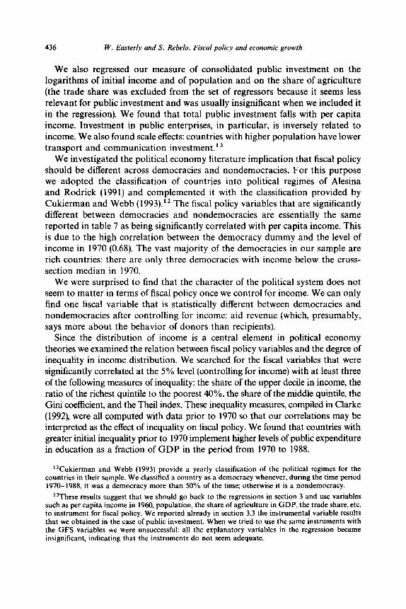
Our data source was the large collection of World Bank reports on public investment in individual countries since 1960. An earlier exercise [Pfeffermann and Madarassy (199111 collected consolidated public investment from a selec- tion of these reports. We expanded this list to more countries and more years: our data set comprises observations on public investment for 36 countries in the 60s 108 countries in the 70s and 119 countries in the 80s. More importantly, we collected data on public investments by sector and by levels of government from these reports, the first time we are aware that this has been done comprehen- sively. We have supplemented the data we collected for aggregate public investment with other sources, including Pfeffermann and Madarassy (1991), the World Bank (1991), and the United Nations national accounts. Our public investment series can be found in the appendix.

The correlation between Central Government Investment and Consolidated Public Sector Investment in the 1980s (the decade for which our data set is more complete) is 0.63, while the median difference between the two rates of investment is 7 percentage points of GDP.

We constructed decade-average public investment ratios by sector from the available data in each decade and entered them into pooled regressions of decade-average per capita growth. We performed regressions using decade averages because of the sparseness of the data. The information on public investment is often available for too few years to allow us to compute meaning- ful averages over periods that are longer than a decade.

We used a similar set of conditioning variables in these regressions as in section 3.1. This set of variables comprises the initial level of income, and decade averages of: primary and secondary enrollment, measures of political instability (assassinations, revolts and coups, and war casualties), and the ratio of government consumption to GDP.9 We extend this regression to include one public investment variable at a time. We report three sets of results in table 5: the basic regression, in which the conditioning variables are the Barro regressors, a version of this regression in which we include the ratio of M2 to GDP as explanatory variable, and another version of the regression in which both the value of M2/GDP and of the trade share in 1970 are included in the right-hand side. In table 6 we repeat the same analysis with private investment as the

‘Government consumption serves as a proxy for taxes collected and then dissipated unproduc- tively as in Barro (1991). When we used our other tax measures instead of government consumption, the number of observations was in general greatly reduced and most of the regression coefficients became statistically insignificant.


Table 5

Regressions of per capita growth on public investment and conditioning variables (pooled regressions with decade averages).

Ratios to GDP

Total consolidated public investment

Sectoral public investment:

Agriculture

Education

Health

Housing and urban infrastructure

Transport and communication

Industry and mining

Public investment by level of government:

General government

Public enterprises

Basic regression Basic regression with M2/GDP

- 0.231 ( - 1.13)

1.490 (2.26)

0.011 (0.02)

1.49 (2.82)

0.661 (2.48)

0.218 (1.39)

0.453 (4.13)

- 0.001 ( - 0.01)

- 0.00007 ( - 0.002)

- 0.34 (- 1.50)

1.10 (1.54)

- 0.304 ( - 1.36)

1.18 (1.60)

- 0.40 - 0.37 ( - 0.54) ( - 0.49)

0.88 0.9 1 ( 1.46) (1.48)

0.588 0.626 (2.53) (2.48)

0.089 0.082 (0.589) (0.53)

0.402 (3.43)

- 0.124 ( - 1.09)

Basic regression with MZ/GDP and trade share

- 0.004 ( - 0.089)

0.388 (3.18)

- 0.13 (- 1.15)

dependent variable. The financial variable is often (but not always) significant in both the private investment and the growth equation. Trade is sometimes significant (especially in the investment regression), but sometimes takes the wrong (negative) sign in the growth regression.

The main results suggested by these regressions are:

(a) Transport and communication investment seem to be consistently positively correlated with growth with a very high coefficient (between 0.59 and 0.66). This type of investment is uncorrelated with private investment suggesting, surprisingly, that it raises growth by increasing the social return to private investment but not by raising private investment itself. Transport and communication investment is still significant in the growth regression when we control for private investment.

@I Total public investment, as well as public enterprise investment, is consistently negatively correlated with private investment. This result can,


Table 6

Regressions of private investment on public investment and conditioning variables (pooled regressions with decade averages).

Ratios to GDP

Total consolidated public investment

Sectoral public investment:

Agriculture

Education

Health

Housing and urban infrastructure

Transport and communication

Industry and mining

Public investment by leuel of government:

General government

Public enterprises

Basic regression Basic regression with M2/GDP

Basic regression with MZ/GDP and trade share

- 0.194 - 0.223 - 0.241 ( - 2.08) ( - 2.19) ( - 2.57)

- 0.943 - 0.66 ( - 2.64) ( - 1.98)

1.987 2.28 (1.29) (1.56)

0.027 2.56 (0.02) (2.31)

2.108 1.26 (1.65) (1.00)

0.001 0.053

(0.00) (0.13)

- 0.351 (- 1.35)

- 0.449 (- 1.37)

- 0.74 ( - 2.24)

1.96 (1.40)

2.29 (1.95)

I.01 (0.85)

- 0.17 ( - 0.43)

- 0.359 ( - 1.14)

I .008 0.775 0.771 (3.89) (2.89) (2.88)

- 0.623 - 0.630 - 0.630 ( - 3.40) ( - 3.07) ( - 3.04)

however, be an artifact introduced by the fact that we constructed our private investment series by subtracting our public investment measure from total investment. Total public enterprise investment seems to have no effect on growth.

(c) General government investment is consistently positively correlated with both growth and private investment, with a coefficient of about 0.4 on growth and near 1 on private investment.

(d) Agriculture investment is consistently negatively related to private investment with a coefficient between - 0.64 and - 0.94.

An important qualification of our results is that we cannot exclude the possibility that the association between public investment and growth is due to reverse causation: public investment may simply be higher in periods of fast expansion.


One piece of indirect evidence against reverse causation is that only transport and communication investment and general government investment are robustly correlated with growth (the association between education and housing investment and growth is not robust). If the direction of causation were from growth to public investment, we would expect all types of public investment to be associated with growth.

In order to investigate whether reverse causation is responsible for our results, we instrument for the public investment variables.” Fortunately, we have a natural set of instruments to use: as we will see in the next section, public investment and other fiscal variables depend on structural country characteristics like initial income, population size, and share of agriculture in GDP. Initial income is already in our basic growth regression, but the latter two variables are plausibly excluded from the growth regression. We also use continent dummies for Africa and Latin America because they are obviously exogenous and may be able to capture region-specific aspects of public investment.

The results on agriculture and public enterprise investment crowding out private investment do not remain significant in the instrumental variables regressions.

The effect of transport and communications on growth is robustly significant with instrumental variables, but the size of the coefficients is disturbingly high: we obtain a coefficient of 2 for transport and communication investment and a coefficient of 0.7 for general government investment. This seems to be a common puzzling feature of aggregate empirical work on infrastructure: Aschauer (1989) and Canning and Fay (1993) also report extremely high coefficients on infrastructure measures in growth regressions.” A study by Bandyopadhyay and Devarajan (1993) lends some credence to the idea that public investment in transport and communication has high returns. These authors report that ex post rates of return to World Bank projects in transport and communication are much higher than those in other sectors, even without considering indirect benefits.

4. Is fiscal policy endogenous?

There are two branches of theoretical literature that suggest the presence of strong endogeneity elements in the choice of fiscal policy, implying that the regressions that we reported in section 3 are contaminated by simultaneous equations bias. The first of these branches studies the optimal fiscal policy,

“We also ran the same regressions lagging the public investment variables one decade. This reduced dramatically the dimension of our sample, rendering almost all variables (including noninvestment variables) insignificant.

“These results contrast, however, with the findings of Holtz-Eakin (1992) who finds no impact of public capital on productivity growth after controlling for fixed effects across US states.


usually under the assumption that the government seeks to maximize the welfare of the representative agent [see, e.g., Charnley (1986), Lucas (1990), and Jones, Manuelli, and Rossi (1993)]. Barro (1990) discusses the implications of fiscal policy being chosen optimally in the context of a specific model. In his model there is an inverted U-shape relation between the share of government expenditures in GDP and the rate of growth whenever the rate of income tax is chosen randomly. In contrast, if governments choose the optimal income tax rate, the relation between the share of government and the rate of growth can be significantly weakened.

The second branch of research that makes policy endogenous treats it as the outcome of a political process [see, e.g., Persson and Tabellini (1991), Cohen and Michel (1991) and Alesina and Rodrick (1991)]. This ‘political economy’ approach points to very few exogenous factors that can be used in the empirical analysis but has an implication that we examine below: democracies and nondemocracies should, in general, implement different policies. We also discuss the relation between policy variables and inequality, since this relation is at the core of many political economy models.

We have seen in section 3 that there is collinearity between certain elements of fiscal policy and initial income. Below we explore in more detail this and other possible determinants of fiscal policy.

4.1. Cross-section evidence 1970-88

Table 7 displays the correlations between fiscal variables and the logarithm of real per capita GDP in 1970 that are statistically significant. This table shows that developed countries tend to rely more on income and consumption taxes and less on international trade taxes. These patterns of association between the level of development and the character of the fiscal system are similar to those identified by Tanzi (1987, 1992) and discussed in Burgess and Stern (1993). In addition, the cross-section data suggests that health and social security expenditures increase with the level of income, while most other types of government expenditures are negatively associated with the level of development.

To investigate the presence of scale effects we regressed our fiscal variables on the values in 1970 of the logarithm population, the logarithm of real per capita GDP, the trade share, and the share of agriculture in GDP [the latter variable was found by Tanzi (1992) to be highly correlated with the fiscal structure]. We found that the ratio of social security contributions to total revenue is positively related to population, while the revenue share of taxes on international trade is negatively related to population. On the expenditure side, we also found strong scale effects: the share of public spending on capital formation, transport and communication, agriculture, and general public services falls with increased


Table 7

Significant correlations of fiscal structure variables with the log of per capita income in 1970.

Averages, 1970-88

Aggregate variables: Consolidated public sector surplus/GDP Total revenue/GDP Grants/GDP Total expenditure and lending minus repayments/GDP

Revenue components as share of total revenue (excluding grants): Tax revenue Nontax revenue

0.49 0.55

- 0.27 0.35

Taxes on income, profits, and capital gains Social security contribution Taxes on international trade and transactions Payroll taxes

0.21 - 0.17

0.35 0.58

- 0.75 0.3 1

Expenditure components as share of total expenditure: General public services Education Health Social security and welfare Recreation, culture, and religion Agriculture, forestry, fishing, and hunting Fuel and energy Transportation and communication

- 0.59 - 0.41

0.36 0.78

- 0.28 - 0.54 - 0.32 - 0.32

Sicat- Virmani statutory tax rates: On 0.75 x average family income On average family income On 2 x average family income On 3 x average family income

0.46 0.47 0.46 0.44

Other variables: Ratio of individual income taxes to personal income 0.59 Ratio of income taxes to GDP 0.51 Ratio of domestic taxes to consumption plus investment 0.48 Ratio of trade taxes to exports plus imports - 0.77 Standard deviation of ratio of trade taxes to exports plus imports - 0.50 ‘Marginal’ tax rate [Koester-Kormendi (1989)] 0.30 ‘Marginal’ tax rate from regression of tax revenue on GDP 0.39

population size. In contrast, the share of defense is positively associated with population size.

These scale effects associated with government expenditures are likely to be related to nonconvexities in either the benefits or the costs of publicly provided goods and services. If a government service has the nonrival consumption property of a pure public good - defense is the classic example - then there is more incentive to provide it in a large scale economy, On the other hand, if there are high setup costs but low marginal costs to providing a particular public service, then the amount of spending per capita for a given per capita level of that service would fall with increased scale.

436 W. Easierly and S. Rebelo, Fiscal policy and economic growth

We also regressed our measure of consolidated public investment on the logarithms of initial income and of population and on the share of agriculture (the trade share was excluded from the set of regressors because it seems less relevant for public investment and was usually insignificant when we included it in the regression). We found that total public investment falls with per capita income. Investment in public enterprises, in particular, is inversely related to income. We also found scale effects: countries with higher population have lower transport and communication investment.i3

We investigated the political economy literature implication that fiscal policy should be different across democracies and nondemocracies. For this purpose we adopted the classification of countries into political regimes of Alesina and Rodrick (1991) and complemented it with the classification provided by Cukierman and Webb (1993).i2 The fiscal policy variables that are significantly different between democracies and nondemocracies are essentially the same reported in table 7 as being significantly correlated with per capita income. This is due to the high correlation between the democracy dummy and the level of income in 1970 (0.68). The vast majority of the democracies in our sample are rich countries: there are only three democracies with income below the cross- section median in 1970.

We were surprised to find that the character of the political system does not seem to matter in terms of fiscal policy once we control for income. We can only find one fiscal variable that is statistically different between democracies and nondemocracies after controlling for income: aid revenue (which, presumably, says more about the behavior of donors than recipients).

Since the distribution of income is a central element in political economy theories we examined the relation between fiscal policy variables and the degree of inequality in income distribution. We searched for the fiscal variables that were significantly correlated at the 5% level (controlling for income) with at least three of the following measures of inequality: the share of the upper decile in income, the ratio of the richest quintile to the poorest 40%, the share of the middle quintile, the Gini coefficient, and the Theil index. These inequality measures, compiled in Clarke (1992), were all computed with data prior to 1970 so that our correlations may be interpreted as the effect of inequality on fiscal policy. We found that countries with greater initial inequality prior to 1970 implement higher levels of public expenditure in education as a fraction of GDP in the period from 1970 to 1988.

‘*Cukierman and Webb (1993) provide a yearly classification of the political regimes for the countries in their sample. We classified a country as a democracy whenever, during the time period 1970-1988, it was a democracy more than 50% of the time; otherwise it is a nondemocracy.

“These results suggest that we should go back to the regressions in section 3 and use variables such as per capita income in 1960, population, the share of agriculture in GDP, the trade share, etc. to instrument for fiscal policy. We reported already in section 3.3 the instrumental variable results that we obtained in the case of public investment. When we tried to use the same instruments with the GFS variables we were unsuccessful: all the explanatory variables in the regression became insignificant, indicating that the instruments do not seem adequate.

W. Easterly and S. Rebelo, Fiscal policy and economic growth

4.2. Long-run evidence: 1870-1988

In order to investigate further the relation between fiscal policy, development, and the scale of the economy, we constructed a

437

the level of panel that

comprises annual data for the period from 1870 to 1988 and includes a total of 28 countries.14 This data was spliced together from various sources: Mitchell (1975, 1982, 1983) Maddison (1982), and Liesner (1989). To obtain a long-term series for real per capita GDP we used the Summers and Heston (1991) data for the period 1950-1988 and extended it backwards in time using the growth rate of real per capita GDP implied by our historical sources.

We divided income and the various fiscal variables in different classes and plotted the median of income against the median of the various fiscal variables for each class (the dashed lines around the median represent 95% confidence bands). These classes were constructed so as to have an identical number of observations.

We found three interesting (but not surprising) patterns in the evolution of fiscal variables. Fig. 2 shows the remarkable increase in the share of government revenue in national income that has occurred between 1870 and 1988. This increase in the importance of government in the economy has been explored in the large literature on ‘Wagner’s Law’ [see, e.g., Ram (1987)].

Fig. 3 shows that the importance of custom taxes as a source of government revenue declines sharply with the level of income. This decline is particularly striking in the United States, where the importance of custom taxes in revenue drops from about 100% at the end of the 18th century to approximately zero in 1988.” Fig. 4 documents that the importance of the income tax as a source of government revenue rises with income.

Figs. 5 and 6 were constructed by classifying population size and income classified in three classes each and depicting the median share of income and custom tax revenue in overall revenue for the nine resulting classes. These figures show a striking association between population size and the importance of taxes on income and on international trade similar to the one suggested by our cross-section data: countries with higher population tend to resort less to trade taxes and more to income taxes.

Table 8 shows the results of a pooled time-series cross-section regressions in which we try to relate the evolution of the shares of income tax revenue and custom tax revenue in total revenue and the share of government revenue in

14The countries in our sample are: Argentina, Australia, Austria, Belgium, Brazil, Canada, Chile, Colombia, Denmark, Finland, France, Germany, Greece, Italy, Japan, Mexico, Netherlands, New Zealand, Norway, Peru, Portugal, Spain, Sweden, Switzerland, United Kingdom, Uruguay, USA, and Venezuela.

“Our data for the US includes only taxation at the Federal level. The taxation of business activity in general and of banking, in particular, was an important source of revenue in some US states during the 19th century [see Wallis, Sylla, and Legler (1993)].

W. Easterly and S. Rebelo, Fiscal policy and economic growth

0 1000 2000 3000 4000 5000 6000 7Ooa 6000 9000 10000

Per capita Income, 1985 int’l prices

Fig. 2. Wagner’s Law, income and size of government, 1870-88.

GDP to a set of explanatory variables. These variables, measured at the annual frequency, include the logarithm of real per capita GDP, the logarithm of population, dummies for the two World Wars, and a time trend.

The coefficient on the logarithm of real per capita GDP has the expected sign: positive for the income tax and government revenue ratios and negative for the share of custom taxes. There is a significant time trend that points to a gradual increase over time in the importance of government revenue in GNP and of income tax revenue in overall revenue. This trend also suggests a gradual decline in the importance of custom taxes.

Table 8 confirms the result that was already suggested by figs. 5 and 6 and by our cross-section data: the logarithm of population is a significant explanatory variable. Population is positively related to the importance of income taxes and of government revenue, while it is negatively related to the custom revenue share. This effect of population does not disappear when we introduce the share of trade in GNP in the regression, thus suggesting the presence of a scale effect associated with population on the character of the tax system. The trade share is negatively associated with customs revenue, since international trade is important in countries with low customs taxes.

The effects of the level of income and of the level of population on the character of the fiscal system are surely related to the administrative and


0.40

0 0.35

2

f ?! 0.30

c

z = 0.25 C

: x 4 0.20

E g 0.15

J "

6 0.10

!? m

f 0.05

0.00

0.45

f 0.40

i ?! _- 0.35

s m

= 0.30

2

I

Q) 0.25 E 8

= 6 0.20

c

g 0.15

0.10

, I I , ,

0 1000 2000 3000 4000 5000 6000 7000 6000 9000


Fig. 3. Per capita income and share of custom taxes, 1870-88.

l-

0 1000 2000 3000 4000 5000 6mO 7000 6000 go00 106001100012000


Fig. 4. Per capita income and share of income taxes, 1870-88.


Share of curtome taxes in revenue

’ Population

\ Y /

Fig. 5. Income, population size, and share of custom taxes in revenue, 1870-88.

0.35

Incoye;z;are in o.3

rixe

Fig. 6. Income, population size, and share of income taxes in revenue, 1870-88.

Tab

le

8

Pool

ed

cros

s-se

ctio

n tim

e se

ries

re

gres

sion

w

ith

hist

oric

al

data

, 18

70-8

8.”

~___

__

Inco

me

tax

reve

nue

Cus

tom

s ta

x re

venu

e G

over

nmen

t re

venu

e

Tot

al

tax

reve

nue

Tot

al

tax

reve

nue

GN

P __

____

___

~___

~

Con

stan

t -

3.24

1 -

0.15

3 3.

039

5.31

0 -

2.31

0 (

- 6.

573)

(

- 0.

272)

(9

.836

) (1

4.85

2)

(-

16.7

83)

Log

of

rea

l pe

r ca

pita

G

DP

0.06

3 0.

101

- 0.

067

- 0.

041

0.01

7 (7

.590

) (1

0.59

2)

(-

9.19

6)

(-

5.79

1)

(6.2

60)

Log

of

pop

ulat

ion

0.02

1

0.03

2 -

0.03

5 -

0.04

1 0.

003

(5.1

69)

(6.1

57)

(-

10.5

12)

( -

10.9

39)

(2.4

50)

Wor

ld

War

I

- 0.

015

0.02

1 0.

008

- 0.

046

- 0.

029

( -

0.51

6)

(0.5

23)

(0.3

86)

( -

2.02

0)

( -

2.84

6)

Wor

ld

War

II

0.

051

0.03

7 -

0.04

6 -

0.04

3 -

0.00

5 (3

.396

) (2

.100

) (

- 3.

056)

(

- 2.

477)

(

- 0.

833)

Tim

e tr

end

0.00

2 -

0.00

02

- 0.

001

- 0.

002

0.00

1 (5

.490

) ( -

0.

780)

(

- 6.

473)

(

- 11

.858

) (1

5.20

0)

Exp

orts

pl

us

impo

rts/

GN

P -

0.05

5 -

0.09

6 -

(1.8

30)

( -

5.91

6)

Num

ber

of o

bser

vatio

ns

894

696

1560

96

2 13

83

R2

0.31

0.

32

0.23

0.

42

0.37

__

___

___-

“t-s

tatis

tics

in p

aren

thes

es.


compliance costs of taxation. These costs are not small: in a study for Canada, Vaillancourt (1989) estimated that the total private and government operating costs associated with the income tax and the social security payments represent 7.1% of the revenue collected. In a similar study for the UK in the period 1986-87, Sandford, Godwin, and Hardwick (1989) estimated that these costs represent 4.93% of revenue.

It is plausible that custom taxes require little or no overhead expenditures, but are costly to administer per unit of tax collected. Income taxes imply high overhead costs for establishing income reporting, surveillance, and withholding systems, but once such overhead costs are paid, the marginal cost of an additional unit of tax collected is low. Under these circumstances, a government in a small scale economy (low population size, low income, or both) would prefer to use custom taxes, while a government in a large economy would find it worthwhile to bear the fixed costs of collecting income taxes.

5. Further directions

The empirical regularities summarized in this paper suggest a number of lines of further inquiry. One is the influence of economic scale on the choice of fiscal instruments. The literature has often noted the dependence of fiscal structure on income, but has not interpreted this relation as having anything to do with the scale of the economy. Our results on population, income, and fiscal structure suggest that scale matters. In order to be consistent with these scale effects, theoretical analyses of the choice of fiscal systems will have to take into account the cost of administer- ing different tax systems, as well as the lumpiness of some types of expenditures. Distributional objectives are an additional consideration for the design of fiscal system: we found evidence that inequality affects education spending.

The evidence that tax rates matter for growth is disturbingly fragile. This empirical fragility contrasts sharply with the robustness of the theoretical predictions: most growth models predict that income and investment taxes are detrimental to growth. Our results on the dependence of both growth and tax policy on initial income help explain why it is difficult to isolate the effects of tax policy on growth. One avenue for further empirical research is to search for natural experiments in which there are large changes in tax policy, where the covariation with income does not constitute a problem.

Our results on public investment in transport and communication seem to lend support from developing country experiences to Aschauer’s (1989) conten- tion that public spending on infrastructure has supernormal returns. We have some suggestive evidence that causality runs from infrastructure to growth, but further work is necessary to address both causality questions and the surprising high magnitude of coefficients on public infrastructure spending. Much more data collection on infrastructure is needed, given the paucity of data on comprehensive infrastructure spending in most countries; our public investment data set is a beginning in this regard.

App

endi

x

Tab

le A

.1

Sum

mar

y st

atis

tics:

C

ross

-sec

tion

vari

able

s,

1970

-88.

”

Var

iabl

es

Sour

ce

Var

iabl

es e

xpre

ssed

as

per

cent

age of

GD

P:

Cen

tral

go

vern

men

t su

rplu

s C

onso

lidat

ed

publ

ic s

ecto

r su

rplu

s

Rev

enue

: T

otal

rev

enue

and

gra

nts

Tax

es o

n in

com

e, p

rofi

ts,

and

capi

tal

gain

s So

cial

sec

urity

con

trib

utio

ns

Em

ploy

ers

payr

oll

or m

anpo

wer

ta

xes

Tax

es o

n pr

oper

ty

Dom

estic

ta

xes

on g

oods

an

d se

rvic

es

Tax

es o

n in

tern

atio

nal

trad

e an

d tr

ansa

ctio

ns

Oth

er

taxe

s T

otal

rev

enue

T

ax r

even

ue

Non

tax

reve

nue

Cap

ital

reve

nue

Cur

rent

re

venu

e G

rant

s

Exp

endi

ture

s:

Gen

eral

pu

blic

ser

vice

s D

efen

se

Edu

catio

n H

ealth

So

cial

sec

urity

and

wel

fare

H

ousi

ng

and

com

mun

ity

amen

ities

R

ecre

atio

n,

cultu

re,

and

relig

ion

Agr

icul

ture

, fo

rest

ry,

fish

ing,

and

hun

ting

Min

ing,

man

ufac

turi

ng,

and

cons

truc

tion

GFS

98

-

0.04

6 0.

047

0.05

4 E

RS

53

- 0.

050

0.03

8 0.

040

GFS

10

2 0.

265

0.10

8 0.

558

GFS

10

3 0.

060

0.04

8 0.

262

GFS

10

3 0.

031

0.04

1 0.

188

GFS

10

1 0.

002

0.00

6 0.

036

GFS

10

3 0.

005

0.00

6 0.

039

GFS

10

3 0.

058

0.04

0 0.

190

GFS

10

3 0.

043

0.03

9 0.

215

GFS

10

2 0.

005

0.00

7 0.

044

GFS

10

3 0.

243

0.10

5 0.

537

GFS

10

3 0.

203

0.09

2 0.

468

GFS

10

2 0.

038

0.04

3 0.

349

GFS

10

0 0.

001

0.00

3 0.

024

GFS

10

2 0.

242

0.10

5 0.

537

GFS

10

0 0.

021

0.04

3 0.

259

GFS

86

0.

039

0.02

9 0.

142

GFS

86

0.

027

0.03

0 0.

230

GFS

87

0.

034

0.01

8 0.

074

GFS

87

0.

020

0.01

5 0.

068

GFS

86

0.

05 1

0.05

6 0.

208

GFS

86

0.

007

0.00

6 0.

027

GFS

85

0.

004

0.00

4 0.

029

GFS

84

0.

018

0.01

4 0.

076

GFS

84

0.

007

0.01

2 0.

075

No.

of

ob

s.

Mea

n St

d.

dev.

M

ax.

Min

. 3 2

- 0.

222

4 -

0.13

8 $ 9

0.09

6 2

0.00

0 b

0.00

0

0.00

0

8 -2

o.O

OQ

*r

l 0.

000

E.

0.00

0 “a

0.lX

K.l

i 0.

078

$’

0.05

9 g

o.oo

o Q

0.

000

:: 0.

078

2 O

.ooo

$.

: 0.

003

$ 0.

000

P 0.

000

0.00

2 0.

000

0.00

0 0.

000

0.00

0 0.

000

2 LJ

Tab

le A

.1 (

cont

inue

d)

Var

iabl

es

Fuel

and

ene

rgy

Tra

nspo

rt

and

com

mun

icat

ion

Oth

er

expe

nditu

res

Cur

rent

ex

pend

iture

G

ross

fi

xed

capi

tal

form

atio

n C

apita

l ex

pend

iture

T

otal

exp

endi

ture

m

inus

len

ding

plu

s re

paym

ent

Var

iabl

es e

xpre

ssed

as

per

cent

age

of G

DP:

G

over

nmen

t ex

pend

iture

s R

eal

gove

rnm

ent

cons

umpt

ion/

Rea

l G

DP

Gro

ss

real

pub

lic i

nves

tmen

t/Rea

l G

DP

Scat

-Vir

man

i (1

988)

st

atut

ory

tax

rate

s:

On

firs

t in

com

e br

acke

t O

n 0.

75 x

ave

rage

fam

ily i

ncom

e O

n av

erag

e fa

mily

inc

ome

On

2 x

aver

age

fam

ily i

ncom

e O

n 3

x av

erag

e fa

mily

inc

ome

On

high

est

inco

me

brac

ket

Oth

er v

aria

bles

: In

divi

dual

in

com

e ta

xes/

Pers

onal

in

com

e E

aste

rly-

Reb

el0

(199

3) m

argi

nal

inco

me

tax

rate

‘M

argi

nal’

tax

rat

e [K

oest

er-K

orm

endi

(1

989)

] D

omes

tic

taxe

s/C

onsu

mpt

ion

plus

inv

estm

ent

Stan

dard

de

viat

ion

of r

atio

of

dom

estic

ta

xes

to c

onsu

mpt

ion

plus

inv

estm

ent

Inte

rnat

iona

l tr

ade

taxe

s/Im

port

s pl

us e

xpor

ts

Stan

dard

de

viat

ion

of r

atio

of

inte

rnat

iona

l tr

ade

taxe

s to

im

port

s pl

us e

xpor

ts

‘Mar

gina

l’ i

ncom

e ta

x ra

te c

ompu

ted

with

tim

e se

ries

reg

ress

ion

on G

DP

‘Mar

gina

l’ t

ax r

ate

com

pute

d w

ith t

ime

seri

es r

egre

ssio

n of

tax

rev

enue

on

GD

P

Sour

ce

No.

of

ob

s.

Mea

n St

d.

dev.

M

ax.

Min

.

GFS

82

0.

005

0.00

6 0.

025

0.000

GFS

84

0.

023

0.01

7 0.

121

0.000

GFS

84

0.

013

0.01

3 0.

069

0.00

1 G

FS

94

0.23

4 0.

104

0.61

4 0.

078

GFS

79

0.

033

0.03

2 0.

220

0.00

0 G

FS

94

0.05

8 0.

049

0.32

5 0.

000

GFS

97

0.

308

0.12

0 0.

702

0.10

8

SH

48

0.30

0 0.

107

0.51

9 0.

098

BW

11

2 0.

187

0.06

8 0.

380

0.04

7 B

W

98

0.10

8 0.

054

0.24

5 0.

001

51

18.8

14

17.3

78

66.0

00

0.00

0 51

8.

688

8.52

1 36

.000

0.

000

51

15.0

65

15.6

44

60.0

00

0.00

0 52

28

.502

19

.029

71

.000

2.

200

52

34.1

87

20.0

35

95.5

00

2.20

0 52

61

.552

15

.507

95

.500

25

.Ot?

O

80

0.03

9 0.

037

0.13

6 0.

000

32

0.06

4 0.

05 I

0.18

7 0.

001

63

0.30

8 0.

221

0.14

2 -

0.00

8 82

0.

074

0.05

1 0.

215

0.00

9 82

0.

014

0.01

3 0.

079

0.00

2 89

0.

065

0.04

5 0.

192

0.00

1 89

0.

018

0.01

5 0.

080

0.00

1 60

0.

109

0.09

9 0.

376

0.00

2 69

0.

293

0.17

9 0.

826

- 0.

123

“Sou

rces

: G

FS [

Gov

ernm

ent

Fina

ncia

l St

atis

tics]

, B

W [

Bar

ro

and

Wol

f (1

989)

], S

H [

Sum

mer

s an

d H

esto

n (1

991)

], E

RS

[Eas

terl

y,

Rod

rigu

ez,

and

Schm

idt-

Heb

bel

(199

311.

Tab

le A

.2

Sum

mar

y st

atis

tics:

Pu

blic

in

vest

men

t va

riab

les

(dec

ade

aver

ages

, 19

6Os,

197

Os,

and

1980

s).

____

_ -_

__-

____

__

__

~___

No.

of

Std.

V

aria

bles

exp

ress

ed

as p

erce

ntag

e of

GD

P ob

s.

Mea

n de

v.

Max

. M

in.

Agg

rega

te

data

: T

otal

con

solid

ated

pu

blic

inv

estm

ent

Priv

ate

inve

stm

ent

Publ

ic e

nter

pris

e in

vest

men

t Pu

blic

inv

estm

ent

by g

ener

al g

over

nmen

t

258

0.09

17

0.05

22

0.32

68

0.01

82

212

0.11

93

0.06

68

0.44

05

0.00

55

99

0.04

24

0.02

50

0.13

26

0.00

24

121

0.05

19

0.03

34

0.20

14

0.01

54

Sect

oral

da

ta:

Publ

ic i

nves

tmen

t in

tra

nspo

rt

and

com

mun

icat

ion

112

0.02

24

0.01

52

0.10

26

0.00

12

Publ

ic i

nves

tmen

t in

agr

icul

ture

13

3 0.

0144

0.

0932

Pu

blic

inv

estm

ent

in e

duca

tion

0.01

26

0.00

02

121

0.00

60

0.00

57

0.03

76

0.00

02

Publ

ic i

nves

tmen

t in

hea

lth

111

0.00

37

0.00

38

0.02

41

0.00

02

Publ

ic i

nves

tmen

t in

hou

sing

an

d ur

ban

infr

astr

uctu

re

88

0.00

56

0.00

66

0.03

41

O.O

fKlO

Pu

blic

inv

estm

ent

in i

ndus

try

and

min

ing

89

0.01

31

0.01

76

0.10

71

0.00

00

____

~ ~_

_~

__~

~~~

Tab

le

A.3

Sum

mar

y st

atis

tics:

H

isto

rica

l da

ta

set.

Cou

ntry

Pe

riod

Per

capi

ta

GD

P (U

S$

in

1985

pp

p pr

ices

)

Lev

el

at

begi

nnin

g of

pe

riod

Arg

entin

a A

ustr

alia

A

ustr

ia

Bel

gium

B

razi

l C

anad

a C

hile

C

olom

bia

Den

mar

k Fi

nlan

d Fr

ance

G

erm

any

Gre

at

Bri

tain

G

reec

e It

aly

Japa

n M

exic

o N

ethe

rlan

ds

New

Z

eala

nd

Nor

way

Pe

ru

Port

ugal

Sp

ain

Swed

en

Switz

erla

nd

Uru

guay

U

SA

Ven

ezue

la

1900

-198

8 17

52

4030

19

3551

975

8%

1890

-198

8 39

09

1332

1 19

01-1

986

18%

18

70-1

988

1273

11

201

1924

-197

5 18

%

1870

-198

8 20

66

1149

5 19

24-1

975

19%

18

70-1

987

331

4441

18

70-1

975

9%

1870

-198

8 17

92

1627

2 19

26-1

988

26%

19

08-1

988

1706

40

99

1940

-197

5 14

%

1925

-198

8 96

6 35

68

1945

-197

5 8%

18

70-1

988

1403

12

089

1870

-197

5 6%

18

70-1

988

824

1236

0 19

26-1

975

20%

18

70-1

988

1373

12

190

1949

-197

5 22

%

1870

-198

8 12

35

1260

4 18

7221

975

7%

1870

-198

8 22

23

1198

2 18

85-1

975

18%

19

50-1

988

1225

58

57

1928

-197

5 17

%

1870

-198

8 14

17

1174

1 18

70-1

975

12%

19

30-1

988

1596

12

209

1930

-198

6 15

%

1895

5198

8 11

13

4996

19

26-1

975

8%

1900

-198

8 24

00

1146

8 19

00-1

975

9%

1950

-198

8 56

08

9864

19

31-1

975

26%

18

70-1

988

1117

14

976

1870

-197

5 7%

19

50-1

988

1642

28

47

1942

-197

5 13

%

1870

-198

8 48

7 53

21

1879

-197

5 11

%

1950

-198

8 18

23

7406

19

06-1

975

9%

1870

-198

8 92

6 12

991

#N/A

#

N/A

18

70-1

988

2316

16

155

1913

3198

8 7%

19

35-1

988

3186

51

63

1955

-197

5 11

%

1870

-198

8 20

67

1833

9 18

8991

975

5%

1950

-198

7 29

21

5717

19

50-1

975

23%

Lev

el

at

end

of p

erio

d

Gov

ernm

ent

reve

nue

shar

e in

GD

P

Peri

od

Med

.

4%

12%

2%

28

%

9%

24%

13

%

25%

6%

22

%

14%

41

%

14%

21

%

5%

11%

6%

33

%

9%

28%

2%

24

%

2%

31%

6%

38

%

11%

21

%

4%

17%

11

%

28%

6%

13

%

5%

34%

17

%

35%

3%

21

%

11%

17

%

5%

16%

5%

15

%

# N

/A

#N/A

2%

11

%

10%

15

%

1%

23%

19

%

36%

Max

.

Tab

le A

.3 (

cont

inue

d)

Cus

tom

s ta

x sh

are

in r

even

ue

Inco

me

tax

shar

e in

rev

enue

Cou

ntry

Pe

riod

Arg

entin

a 19

85-1

975

Aus

tral

ia

# N

/A

Aus

tria

18

70-1

975

Bel

gium

18

70-1

955

Bra

zil

1900

-197

5 C

anad

a #N

/A

Chi

le

1895

-197

5 C

olom

bia

1928

-197

5 D

enm

ark

1891

-197

5 Fi

nlan

d 18

83-1

975

Fran

ce

1870

-197

5 G

erm

any

1872

-197

5 G

reat

B

rita

in

1870

-196

4 G

reec

e #N

/A

Ital

y 18

70-1

975

Japa

n #N

/A

Mex

ico

1925

-197

5 N

ethe

rlan

ds

1870

-197

5 N

ew Z

eala

nd

1870

-197

5 N

orw

ay

1870

-197

5 Pe

ru

1899

-197

5 Po

rtug

al

1879

-197

5 Sp

ain

1870

-197

5 Sw

eden

18

81-1

975

Switz

erla

nd

1870

-197

5 U

rugu

ay

1895

5197

5 U

SA

1870

-197

5 V

enez

uela

19

10-1

975

Med

. M

in.

48%

29

%

#N/A

#

N/A

6%

0%

8%

1%

31

%

3%

#N/A

#N

/A

41%

6%

28

%

12%

17

%

1%

35%

2%

11

%

0%

13%

0%

21

%

9%

#N/A

#N

/A

8%

0%

#N/A

#

N/A

24

%

10%

8%

0%

28

%

6%

37%

1%

25

%

8%

32%

10

%

12%

4%

17

%

2%

65%

11

%

58%

6%

15

%

1%

34%

3%

Max

. Pe

riod

M

ed.

Min

. M

ax.

71%

#

N/A

25

%

17%

64

%

#N/A

10

0%

56%

49

%

51%

27

%

36%

29

%

#N/A

15

%

# N

/A

39%

22

%

46%

76

%

39%

44

%

22%

50

%

100%

10

0%

60%

10

0%

1895

-197

5 19

49-1

986

# N

/A

# N

/A

1923

-197

5 19

18-1

986

1895

-197

5 19

28-1

975

1870

-197

5 19

34-1

975

# N

/A

1920

-197

5 #

N/A

#N

/A

# N

/A

1887

-198

6 19

25-1

975

# N

/A

1893

-197

5 18

93-1

975

# N

/A

#N/A

#

N/A

18

81-1

975

1916

-197

5 #

N/A

19

16-1

975

#N/A

16%

38

%

# N

/A

#N/A

26

%

21%

26

%

44%

24

%

30%

#N

/A

44%

#

N/A

#N

/A

# N

/A

14%

26

%

# N

/A

23%

21

%

#N/A

#N

/A

# N

/A

25%

24

%

# N

/A

63%

#N

/A

2%

28%

#

N/A

#

N/A

2%

3%

1%

5%

12

%

17%

#

N/A

22

%

#N/A

#

N/A

#

N/A

1%

9%

#

N/A

2%

6%

#

N/A

#

N/A

#

N/A

5%

6%

#

N/A

17

%

#N/A

37%

45

%

# N

/A

#N/A

*3

8%

32%

52

%

56%

64

%

37%

#

N/A

59

%

# N

/A

# N

/A

#N/A

40

%

42%

#

N/A

70

%

90%

#

N/A

#

N/A

#N

/A

55%

82

%

# N

/A

76%

#N

/A

Tab

le A

.4

Publ

ic i

nves

tmen

t da

ta (

all

seri

es a

re d

ecad

e av

erag

es e

xpre

ssed

as

rat

io

to G

NP)

; 19

60s

1970

s an

d 19

80s.

No.

C

ount

ry

I A

ntig

ua a

nd

Bar

buda

2

Arg

entin

a 3

Aus

tral

ia

4 A

ustr

ia

5 B

aham

as

6 B

angl

ades

h 7

Bar

bado

s 8

Bel

ize

9 B

enin

10

Bol

ivia

11

Bot

swan

a 12

Bra

zil

13 B

ulga

ria

14 B

urki

na F

aso

15 B

urun

di

16 C

amer

oon

17 C

anad

a 18

Cen

tral

A

fric

an

Rep

. 19

Cha

d 20

Chi

le

21 C

hina

22

Col

ombi

a 23

Com

oros

24

Con

go

25 C

osta

Ric

a

Tot

al c

onso

lidat

ed

publ

ic i

nves

tmen

t

60s

70s

80s

Priv

ate

inve

stm

ent

60s

70s

80s

0.05

4 0.

087

0.07

6

0.08

2 0.

050

0.05

3 0.

057

0.09

5 0.

082

0.11

0 0.

091

0.15

6 0.

083

0.13

6 0.

039

0.07

3 0.

114

0.06

2 0.

068

0.02

3 0.

078

0.04

6 0.

080

0.05

6 0.

060

0.14

6 0.

063

0.18

6 0.

094

0.13

7 0.

153

0.14

3 0.

126

0.16

9

0.34

4 0.

137

0.04

6

0.17

6 0.

045

0.07

1 0.

080

0.24

6 0.

140

0.01

3 0.

013

0.07

9

0.20

4 0.

087

0.17

7

0.05

9

0.11

6 0.

065

0.04

5 0.

253

0.12

6 0.

152

0.19

1 0.

014

0.08

5

0.05

5 0.

099

0.10

3 0.

115

0.02

6 0.

073

0.07

9 0.

060

0.07

0 0.

097

0.18

1 0.

178

0.16

3 0.

169

0.04

1 0.

055

0.07

4 0.

154

0.10

5 0.

099

0.20

9 0.

065

0.13

0 0.

117

0.10

1 0.

044

0.06

9 0.

066

0.13

7 0.

155

0.13

8

Publ

ic

ente

rpri

se

Publ

ic i

nves

tmen

t by

in

vest

men

t ge

nera

l go

vern

men

t

60s

70s

80s

60s

70s

80s

0.03

9 0.

041

0.03

7 0.

027

0.04

8 0.

034

0.02

0 0.

036

0.06

8 0.

055

0.04

2 0.

045

0.04

1

0.02

5 0.

063

0.07

7 0.

115

0.01

9 0.

032

0.03

3 0.

027

0.03

1

0.04

3

0.03

3 0.

037

0.03

8 0.

035

0.01

7 0.

026

0.02

6

Sect

oral

pu

blic

in

vest

men

t in

tra

nspo

rt

and

com

mun

icat

ions

60s

70s

80s

0.04

3

0.03

0 0.

027

0.11

0 0.

112

0.02

5 0.

084

0.03

8 0.

014

0.02

3 0.

039

0.02

9 0.

02 1

0.

010

0.01

7 0.

038

0.05

3 0.

034

0.02

6

0.02

3 0.

017

0.01

3 0.

103

26 C

ote

d’Iv

oire

27

Cyp

rus

28 D

omin

ica

29 D

omin

ican

R

ep.

30 E

cuad

or

31 E

gypt

32

El

Salv

ador

33

Equ

ator

ial

Gui

nea

34 E

thio

pia

35 F

iji

36 G

abon

37

Gha

na

38 G

reec

e 39

Gre

neda

40

Gua

tem

ala

41 G

uine

a 42

Gui

nea

Bis

sau

0.07

8 0.

141

0.04

0 0.

137

0.06

5 0.

078

0.17

1 0.

052

0.05

2 0.

094

0.12

0 0.

048

0.06

5

0.07

6 0.

050

0.15

3 0.

052

0.08

7 0.

183

0.04

5

0.08

9 0.

082

0.10

3 0.

143

0.13

2 0.

051

0.11

7

0.04

0 0.

162

0.19

5

0.20

2

0.09

9

0.21

5 0.

166

0.07

1

0.05

3 0.

029

0.01

2 0.

017

0.02

9 0.

028

0.05

3 0.

077

0.04

3

0.09

9 0.

046

0.05

2

0.03

1

0.08

6 0.

07s

0.09

9

0.05

2 0.

026

0.05

4 0.

052

0.11

3 0.

011

0.02

2 0.

028

0.04

9 0.

011

0.01

4

0.01

8

0.04

4 0.

008

0.02

7 0.

017

0.08

1

0,03

6 0.

019

0.13

1 0.

175

0.04

1 0.

123

0.17

9

0.10

7 0.

019

0.03

8 0.

060

0.09

7

0.13

1 0.

103

0.08

9 0.

141

0.04

3 0.

067

0.20

3 0.

041

0.06

2 0.

291

0.13

1

0.03

7 0.

024

0.04

7 0.

027

0.04

7 0.

052

0.02

9 0.

039

0.03

3 0.

016

0.02

9 0.

041

0.01

1 0.

010

0.04

7 0.

028

0.00

6 0.

026

0.01

6 0.

026

0.09

7 0.

119

0.09

8 0.

020

0.06

2

0.13

0

0.03

3

0.04

8 0.

035

0.02

9 0.

026

43 G

uyan

a 44

Hai

ti 45

Hon

dura

s 46

Hon

g K

ong

47 H

unga

ry

48 I

cela

nd

49 I

ndia

50

Ind

ones

ia

51 I

srae

l 52

Jam

aica

53

Jap

an

54 J

orda

n 55

Ken

ya

56 K

orea

57

Lao

, Pe

ople

’s

Dem

. R

ep.

58 L

eban

on

59 L

esot

ho

60 L

iber

ia

61 L

ibya

62

Mad

agas

car

0.10

7 0.

021

0.03

5

0.17

3 0.

064

0.05

6 0.

035

0.29

7 0.

046

0.22

7 0.

08 1

0.

062

0.05

3 0.

155

0.26

5

0.04

7 0.

054

0.03

0 0.

018

0.06

0 0.

079

0.03

9 0.

031

0.05

9 0.

084

0.04

3 0.

207

0.03

6 0.

100

0.10

2 0.

039

0.12

4 0.

079

0.14

6 0.

084

0.07

0

0.11

0.

260

0.03

7

0.06

7 0.

07 t

0.08

3 0.

127

0.09

3 0.

126

0.16

4

0.23

7

0.10

1 0.

024

0.10

9 0.

055

0.03

8 0.

048

0.02

8 0.

047

0.05

5 0.

054

0.04

0

0.01

1 0.

058

0.10

8 0.

098

0.09

2 0.

176

0.02

0 0.

212

0.07

3 0.

025

0.03

2 0.

038

0.05

4

0.08

7 0.

059

0.12

7 0.

t 18

0.

196

0.22

1 0.

050

0,02

6 0.

017

0.07

6

0.15

1

0.19

4

0.03

5 0.

032

0.15

5

0.20

1

0.11

7 0.

137

0.07

8 0.

079

0.05

8 0.

078

0.23

4

Tab

le A

.4 (

cont

inue

d)

Sect

oral

pu

blic

in

vest

men

t in

tra

nspo

rt

and

com

mun

icat

ions

T

otal

con

solid

ated

pu

blic

inv

estm

ent

No

. C

ount

ry

60s

70s

80s

63 M

alaw

i 0.

075

64 M

alay

sia

65 M

ali

66 M

alta

67

Mau

rita

nia

0.08

6 68

Mau

ritiu

s 69

Mex

ico

70 M

onts

erra

t 71

Mor

occo

0.

081

72 M

ozam

biqu

e 73

Mya

nam

ar

(Bur

ma)

0.

072

74 N

epal

75

Net

herl

ands

76

New

Zea

land

77

Nic

arag

ua

0.04

1 78

Nig

er

0.04

3 79

Nig

eria

80

Nor

way

81

Pak

ista

n 82

Pan

ama

0.04

0 83

Pap

ua

New

G

uine

a 84

Par

agua

y 0.

044

85 P

eru

0.04

2 86

Phi

lippi

nes

87 P

olan

d 88

Por

tuga

l 89

Rw

anda

90

Sao

Tom

e an

d Pr

inci

pe

0.13

4 0.

081

0.02

1 0.

091

0.12

2 0.

076

0.07

7 0.

125

0.11

7

0.06

9 0.

043

0.08

6 0.

062

0.05

1 0.

062

0.09

1 0.

093

0.05

9 0.

077

0.08

3 0.

056

0.10

8 0.

087

0.13

7 0.

160

0.12

4

0.09

0 0.

067

0.17

9 0.

019

0.05

0 0.

063

0.09

2 0.

147

0.18

4 0.

039

0.02

5 0.

050

0.05

6 0.

088

0.11

8 0.

154

0.04

8 0.

033

0.05

2 0.

055

0.17

4 0.

144

0.01

2 0.

024

0.07

3 0.

202

0.01

4 0.

111

0.11

9 0.

104

0.20

7 0.

086

0.07

8 0.

027

0.09

8 0.

104

0.09

9 0.

146

0.14

5 0.

060

0.27

1 0.

077

0.07

6 0.

094

0.10

0 0.

153

0.12

6 0.

077

0.06

8

0.08

9 0.

124

0.11

1

Priv

ate

inve

stm

ent

60s

70s

80s

Publ

ic e

nter

pris

e in

vest

men

t

60s

70s

80s

Publ

ic i

nves

tmen

t by

ge

nera

l go

vern

men

t

60s

70s

80s

0.06

3 0.

090

0.14

3

0.14

5 0.

131

0.16

9 0.

192

0.12

6 0.

232

0.04

3 0.

079

0.16

7 0.

094

0.10

5

0.05

1 0.

159

0.00

9 0.

055

0.10

6 0.

199

0.02

4 0.

029

0.04

7 0.

002

0.13

3 0.

128

0.27

6 0.

122

0.01

8 0.

016

0.01

4 0.

043

0.03

4 0.

050

0.13

3 0.

102

0.14

7 0.

131

0.02

7 0.

045

0.00

5 0.

047

0.03

4

0.07

7 0.

081

0.08

1 0.

096

0.06

8 0.

030

0.09

1 0.

089

0.07

5

0.06

4 0.

082

0.05

5

0.03

8 0.

019

0.03

0

0.03

9 0.

027

0.03

0

0.12

3 0.

047

0.03

3 0.

035

0.03

6

0.04

2 0.

020

0.02

3 0.

029

0.05

0 0.

033

0.02

9 0.

041

60s

70s

80s

0.02

5 0.

035

0.03

3 0.

018

0.02

8

0.00

6 0.

024

0.01

4 0.

010

0.01

4 0.

015

0.02

3 0.

015

0.01

0 0.

009

0.01

2 0.

014

0.01

8 0.

019

0.00

7

91 S

eneg

al

92 S

eych

elle

s 93

S

ierr

a L

eon

e 94

Sin

gapo

re

95

Sol

oman

Isl

ands

96

S

outh

Afr

ica

97

Spa

in

98 S

ri L

anka

99

S

t C

hri

stop

her

an

d N

evis

10

0 S

t L

ucia

10

1 S

t. V

ince

nt

102

Su

dan

10

3 S

uri

nam

e 10

4 S

waz

ilan

d 10

5 S

wed

en

106

Syr

ia

107

Tai

wan

10

8 T

anza

nia

109

Tha

ilan

d 11

0 T

he

Gam

bia

111

Tog

o 11

2 T

rini

dad

and

Tob

ago

113

Tun

isia

11

4 T

urk

ey

115

U.S

.A

116

Uga

nda

11

7 U

nit

ed K

ingd

om

118

Uru

guay

11

9 V

enez

uel

a 12

0 Y

emen

, A

rab

Rep

. of

12

1 Y

emen

, P

eopR

’s

Dem

. R

ep.

of

122

Yug

osla

via

123

Zai

re

124

Zam

bia

125

Zim

babw

e

0.05

7 0.

061

0.05

1 0.

090

0.08

0 0.

130

0.03

3 0.

073

0.04

0 0.

117

0.05

0 0.

131

0.06

3 0.

101

0.03

0 0.

137

0.11

8 0.

101

0.11

4 0.

052

0.05

3 0.

126

0.05

2 0.

137

0.10

3 0.

068

0.07

9 0.

128

0.12

1

0.05

9

0.07

3

0.14

4

0.08

4

0.11

4

0.05

6 0.

250

0.14

2

0.08

0 0.

100

0.06

1 0.

289

0.25

5 0.

138

0.04

3

0.03

0

0.00

9

0.00

6

0.02

2

0.01

3 0.

065

0.00

8 0.

009

0.01

3 0.

034

0.05

7

0.09

3

0.07

0

0.05

1

0.04

5 0.

078

0.05

6 0.

019

0.04

4

0.03

0 0.

042

0.07

4 0.

086

0.04

0 0.

089

0.12

2

0.01

7 0.

331

0.17

2 0.

086

0.10

6 0.

160

0.13

9 0.

070

0.12

3 0.

101

0.15

9 0.

075

0.11

2

0.10

7

0.02

2

0.05

2

0.02

5 0.

037

0.01

7 0.

007

0.01

5 0.

037

0.09

1 0.

105

0.04

7 0.

093

0.08

6 0.

149

0.12

1 0.

08 1

0.

066

0.08

1

0.12

9

0.44

1 0.

177

0.07

5 0.

184

0.13

0 0.

038

0.13

2 0.

116

0.16

4 0.

076

0.02

8 0.

030

0.03

5 0.

055

0.05

2 0.

018

0.00

9 0.

023

0.24

3

0.04

9 0.

026

0.02

8

0.08

5 0.

064

0.03

6 0.

038

0.04

9 0.

045

0.05

4 0.

038

0.02

2 0.

035

0.04

4 0.

043

0.01

2 O

.CO

9 0.

029

0.02

0 0.

027

0.01

9 0.

036

0.04

9 0.

077

0.05

1

0.16

3 0.

044

0.11

5 0.

101

0.14

4 0.

148

0.10

0 0.

118

0.02

8 0.

022

0.03

2 0.

052

0.07

3 0.

038

0.04

5 0.

042

0.10

4 0.

122

0.10

5 0.

126

0.09

7 0.

098

0.10

6 0.

089

0.05

3 0.

059

0.17

8 0.

176

0.00

8 0.

006

0.11

5 0.

129

0.08

3 0.

071

0.18

2 0.

090

0.03

2 0.

020

0.04

1

0.02

4 0.

023

0.02

4

0.05

0 0.

065

0.01

5

0.01

8 0.

024

0.01

8

0.08

4 0.

084

0.11

1

0.01

9 0.

024

0.04

1 0.

020

0.01

8 0.

056

0.02

3 0.

021

0.02

0 0.

023

0.07

0 0.

136

0.31

0 0.

327

0.25

0 0.

234

0.04

9 0.

043

0.24

6 0.

132

0.07

2 0.

083

0.06

4 0.

054

0.05

3 0.

064

0.02

8 0.

095

0.04

0 0.

032

0.00

1 0.

006

0.01

0

0.01

8

0.03

8 0.

043

0.02

5 0.

094

0.07

0

0.02

1

0.02

8

0.04

7

0.01

8 0.

038

0.04

2 0.

112

0.03

7


-0mo

8 s-n-- 000 dddd

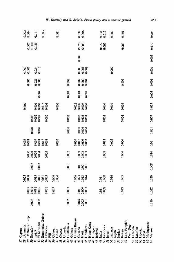
27 C

ypru

s 28

Dom

inic

a 29

Dom

inic

an

Rep

. 30

Ecu

ador

31

Egy

pt

32 E

l Sa

lvad

or

33 E

quat

oria

l G

uine

a 34

Eth

iopi

a 35

Fiji

36

Gab

on

37 G

hana

38

Gre

ece

39 G

rene

da

40 G

uate

mal

a 41

Gui

nea

42 G

uine

a B

issa

u

0.02

5 0.

008

0.00

4 0.

001

0.00

9 0.

007

0.00

3

0.03

4 0.

013

0.00

7 0.

005

0.00

9 0.

016

0.00

2 0.

006

0.00

0 0.

003

0.00

4 0.

008

0.00

3 0.

004

0.00

3

0.00

2

0.02

5 0.

004

0.00

3

0.00

1 0.

003

0.00

2 0.

002

0.00

2

0.00

2

0.01

5 0.

011

0.03

1 0.

023

0.00

9 0.

004

0.00

9 0.

001

0.01

6 0.

004

0.00

3 0.

002

0.01

5 0.

003

0.02

0

0.00

7 0.

003

0.00

3

0.00

2 0.

003

0.00

1 0.

002

0.01

1 0.

009

0.00

1 0.

003

0.00

1 0.

003

0.00

1 0.

002

0.00

4 0.

002

0.00

1 0.

002

0.00

0 0.

002

0.00

1

0.05

6 0.

093

0.01

3 0.

014

0.02

6 0.

015

0.02

3 0.

008

0.00

8 0.

007

43 G

uyan

a 44

Hai

ti 45

Hon

dura

s 46

Hon

g K

ong

47 H

unga

ry

48 I

cela

nd

49 I

ndia

50

Ind

ones

ia

51 I

srae

l 52

Jam

aica

53

Jap

an

54 J

orda

n 55

Ken

ya

57 L

ao,

Peop

le’s

D

em.

Rep

. 58

Leb

anon

59

Les

otho

60

Lib

eria

61

Lib

ya

62 M

adag

asca

r 63

Mal

awi

0.01

6 0.

041

0.00

3 0.

009

0.00

1 0.

003

0.00

1 0.

001

0.00

4 0.

004

0.00

3 0.

003

0.00

3 0.

001

0.00

1

0.00

8 0.

020

0.03

9 0.

003

0.00

6 0.

009

0.00

3

0.01

1 0.

011

0.00

8 0.

008

0.00

8 0.

013

0.01

6 0.

008

0.02

2 0.

009

0.00

3 0.

004

0.00

2 0.

002

0.01

3 0.

005

0.00

4 0.

006

0.00

4 0.

003

0.00

5 0.

007

0.00

1

0.01

6 0.

022

0.02

0 0.

008

0.01

4 0.

011

0.00

1 0.

007

0.00

5 0.

003

0.00

1 0.

001

0.00

5 0.

010

454 W. Easterly and S. Rebelo, Fiscai policy and economic growth

3

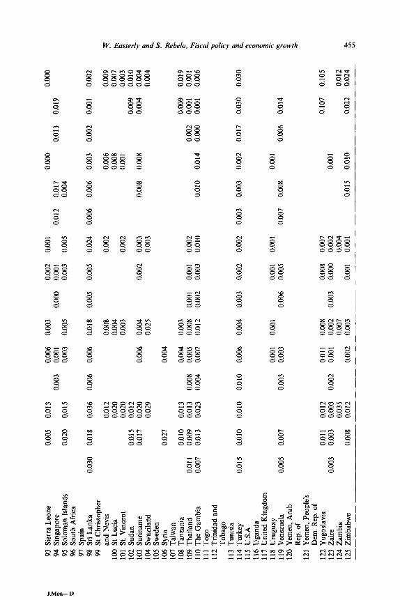
c 93

Sie

rra

Leo

ne

b 94

Sin

gapo

re

b 95

Sol

oman

Is

land

s 96

Sou

th A

fric

a 97

Spa

in

98 S

ri L

anka

99

St

Chr

isto

pher

an

d N

evis

. 10

0 St

Luc

ia

101

St.

Vin

cent

10

2 Su

dan

103

Suri

nam

e 10

4 Sw

azila

nd

105

Swed

en

106

Syri

a 10

7 T

aiw

an

108

Tan

zani

a 10

9 T

haila

nd

110

The

Gam

bia

111

Tog

o 11

2 T

rini

dad

and

Tob

ago

113

Tun

isia

11

4 T

urke

y 11

5 U

.S.A

11

6 U

gand

a 11

7 U

nite

d K

ingd

om

118

Uru

guay

11

9 V

enez

uela

12

0 Y

emen

, A

rab

Rep

. of

12

1 Y

emen

, Pe

ople

’s

Dem

. R

ep.

of

122

Yue

osla

via

123

Za&

e 12

4 Z

ambi

a 12

5 Z

imba

bwe

0.00

5 0.

013

0.00

6 0.

003

0.00

2 0.

001

O.O

C@

0.

000

0.00

3 0.

001

0.00

0 0.

001

0.01

2 0.

017

0.01

3 0.

019

0.02

0 0.

015

0.00

3 0.

005

0.00

3 0.

005

0.00

4

0.03

0 0.

018

0.03

6 0.

006

0.00

6 0.

018

0.00

5 0.

005

0.02

4 0.

006

0.00

6 0.

003

0.01

2 0.

020

0.02

0 0.

015

0.01

2 0.

017

0.02

0 0.

029

0.00

6 0.

004

0.02

5

0.02

7 0.

004

0.01

0 0.

013

0.00

4 0.

003

0.01

1 0.

009

0.01

3 0.

008

0.00

5 0.

008

0.00

7 0.

013

0.02

3 0.

004

0.00

7 0.

012

0.00

8 0.

004

0.00

3

0.00

2 0.

006

0.00

8 0.

002

0.00

1

0.00

2 0.

003

0.00

8 0.

008

0.00

3

0.00

1 0.

001

0.00

2 0.

002

0.00

3 0.

010

0.01

0 0.

014

0.00

2 0.

001

0.00

2

0.00

9 0.

007

0.00

3 0.

009

0.01

0 0.

004

0.00

4 0.

004

0.00

9 0.

019

0.00

2 0.

001

0.00

1 0.

000

0.00

1 0.

006

0.01

5 0.

010

0.01

0 0.

010

0.00

6 0.

004

0.00

3 0.

002

0.00

2 0.

003

0.00

3 0.

002

0.01

7 0.

030

0.03

0

0.00

1 0.

001

0.00

1 0.

001

0.00

1 0.

005

0.00

7 0.

003

0.00

3 0.

006

0.00

5 0.

007

0.00

8 0.

006

0.01

4

0.01

1 0.

012

0.01

1 0.

008

0.00

8 0.

007

0.10

7 0.

105

0.00

3 0.

003

0.00

3 0.

002

0.00

1 0.

002

0.00

3 o.

OO

tl 0.

002

0.00

1 0.

035

0.00

7 0.

004

0.01

2 0.

008

0.01

2 0.

002

0.00

3 0.

001

0.00

1 0.

015

0.01

0 0.

022

0.02

4


References

Alesina, A. and D. Rodrick, 1991, Distributive politics and growth, NBER working paper no. 3668. Alogoskoufis, G. and R. van der Ploeg, 1991, Endogenous growth and overlapping generations,

Mimeo. (Birkbeck College, London). Aschauer, D., 1989, Is public expenditure productive?, Journal of Monetary Economics 23,177-200. Auerbach, A. and L. Kotlikoff, 1987, Dynamic fiscal policy (Harvard University Press, Cambridge,

MA). Azariadis, C. and A. Drazen, 1990, Threshold externalities in economic development, Quarterly

Journal of Economics 105, 501-526. Bandyopadhyay, S. and S. Devarajan, 1993, Using project rates of return to inform sector allocation

decisions, Mimeo. (World Bank, Washington, DC). Barro, R., 1990, Government spending in a simple model of endogenous growth, Journal of Political

Economy 98, S103-S125. Barro, R., 1991, Economic growth in a cross section of countries, Quarterly Journal of Economics

106,407-444. Barro, R. and C. Sahasakul, 1983, Measuring the marginal tax rate from the individual income tax,

Journal of Business 56,419-452. Barro, R. and X. Sala-i-Martin, 1992, Convergence, Journal of Political Economy 100, 223-251. Barro, R. and S. Wolf, 1989, Data appendix for economic growth in a cross-section of countries,

Mimeo. (Harvard University, Cambridge, MA). Becker, G., K. Murphy, and R. Tamura, 1990, Human capital, fertility, and economic growth,

Journal of Political Economy 98, S12-S37. Burgess, R. and N. Stern, 1993, Taxation and development, Journal of Economic Literature 31,

762-830. Canning, D. and M. Fay, 1993, The effect of infrastructure networks on economic growth, Mimeo.

(Columbia University, New York, NY). Cass, D., 1965, Optimum growth in an aggregative model of capital accumulation, Review of

Economic Studies 32, 233-240. Charnley, C., 1986, Optimal taxation of capital income in genera) equilibrium with infinite lives,

Econometrica 54, 6077622. Clarke, G., 1992, More evidence on income distribution and growth, Working paper no. 1064

(World Bank, Washington, DC). Cohen, D. and P. Michel, 1991, Property rights on foreign capital and long run growth, Working

paper no. 9106 (CEPREMAP, Paris). Cukierman, A. and S. Webb, 1993, Political influence on the Central Bank: International evidence,

Mimeo. (World Bank, Washington, DC). Diamond, P., 1965. National debt in a neoclassical growth model. American Economic Review 55.

112551150. Dunn, D. and A. Pellechio, 1990, Analyzing taxes on business income with the effective tax rate

model, Discussion paper no. 79 (World Bank, Washington, DC). Easterly, W. and S. Rebelo, 1993, Marginal income tax rates and economic growth in developing

countries, European Economic Review 37,409-417. Easterly, W., C. Rodriguez, and K. Schmidt-Hebbel, eds., 1993, Public sector deficits and macroeco-

nomic performance (Oxford University Press, Oxford) forthcoming. Easterly, W., M. Kremer, L. Pritchett, and L. Summers, 1993, Good policy or good luck? Country

growth performance and temporary shocks, Journal of Monetary Economics, this issue. Eaton, J., 1981, Fiscal policy, inflation and the accumulation of risky capital, Review of Economic

Studies 48, 4355445. Engen, E. and J. Skinner, 1992, Fiscal policy and growth, NBER working paper no. 4223. Feldstein, M., 1974, Tax incidence in a growing economy with variable labor supply, Quarterly

Journal of Economics 88, 551-573. Fischer, S., 1993, Macroeconomic factors in growth, Journal of Monetary Economics, this issue. Garcia-Mila, 1987, Government purchases and real output: An empirical analysis and equilibrium

model with public capital, Working paper (Universitat Autonoma, Barcelona). Grier, K. and G. Tullock, 1989, An empirical analysis of cross-national economic growth,

1951-1980, Journal of Monetary Economics 87, 225-252.


Holtz-Eakin, D., 1992, Public sector capital and the productivity puzzle, NBER working paper no. 4122.

Jones, L. and R. Manuelh, 1990, A convex model of equilibrium growth: Theory and policy implications, Journal of Political Economy 98, 1008-1038.

Jones, L., R. Manuelli, and P. Rossi, 1993, Optimal taxation in convex models of equilibrium growth, Journal of Political Economy 101,485-517.

Judd, K., 1985, Redistributive taxation in a simple perfect foresight model, Journal of Public Economics 28, 59-83.

King, M. and D. Fullerton, 1984, The taxation of income from capital: A comparative study of the United States, the United Kingdom, Sweden, and West Germany (Chicago University Press, Chicago, IL).

King, R. and R. Levine, 1993, Finance and growth: Schumpeter might be right, Quarterly Journal of Economics 108, 717-737.

King, R. and S. Rebelo, 1993, Transitional dynamics and economic growth in the neoclassical model, American Economic Review, forthcoming.

Koester, R. and R. Kormendi, 1989, Taxation, aggregate activity and economic growth: Cross- country evidence on some supply-side hypotheses, Economic Inquiry 27, 367-386.

Koopmans, T., 1965, On the concept of optimal economic growth, in: The econometric approach to development planning, Pontific Acad. Sci. (North-Holland, Amsterdam) 2255287.

Krzyzaniak, M., 1967, The long run burden of a general tax on profits in a neoclassical world, Public Finance 22, 472-491.

Levine, R. and D. Renelt, 1992, A sensitivity analysis of cross-country growth regressions, American Economic Review 82,942-963.

Liesner, T., 1989, One hundred years of economic statistics (The Economist Publications, London). Lucas, R., 1988, On the mechanics of economic development, Journal of Monetary Economics 22,

3-42. Lucas, R., 1990, Supply side economics: An analytical review, Oxford Economic Papers 42,293-316. Maddison, A., 1982, Phases of capitalistic development (Oxford University Press, Oxford). Mankiw, G., D. Romer, and D. Weil, 1992, A contribution to the empirics of economic growth,

Quarterly Journal of Economics 107, 407-437. Mitchell, B.R., 1978, European historical statistics, 1750-1970 (Columbia University Press, New

York, NY). Mitchell, B.R., 1982, International historical statistics: Asia and Africa (New York University Press,

New York, NY). Mitchell, B.R., 1983, Historical statistics: The Americas and Australasia (Gale Research Co., Detroit,

MI). Persson, T. and G. Tabellini, 1991, Is inequality harmful for growth? Theory and evidence, NBER

working paper no. 3599. Pfeffermann, G. and A. Madarassy, 1991, Trends in private investment in thirty developed countries,

International Finance Corporation discussion paper no. 6 (World Bank, Washington, DC). Plosser, C., 1993, The search for growth in: Federal Reserve of Kansas City symposium series,

Policies for long run growth, 57-86 (Kansas City, MO). Ram, R., 1987, Wagner’s hypothesis in time series and cross section perspectives: Evidence from

‘real’ data for 115 countries, Review of Economics and Statistics, 1944204. Rebelo, S., 1991, Long run policy analysis and long run growth, Journal of Political Economy 99,

500-521. Rivera-Batiz, L. and P. Romer, 1991, International trade with endogenous technical change,

European Economic Review 35, 971-1001. Romer, P., 1986, Increasing returns and long run growth, Journal of Political Economy 94,

100221037. Sandford, C., M. Godwin, and P. Hardwick, 1989, Administrative and compliance costs of taxation

(Fiscal Publications, Bath). Sato, K., 1967, Taxation and neoclassical growth, Public Finance 22, 3466370. Sicat, G. and A. Virmani, 1988, Personal income taxes in developing countries, The World Bank

Economic Review 1, 123-138. Solow, R., 1956, A contribution to the theory of economic growth, Quarterly Journal of Economics

70. 65-94.


Stokey, N. and S. Rebelo, 1993, Growth effects of flat tax rates, Working paper (University of Chicago, Chicago, IL).

Summers, L., 1981, Capital taxation and accumulation in a life-cycle growth model, American Economic Review 71, 533-544.

Summers, R. and A. Heston, 1991, The Penn world table (Mark 5): An expanded set of international comparisons, 1950-1988, Quarterly Journal of Economics 2, 3277368.

Tanzi, V., 1987, Quantitative characteristics of the tax systems of developing countries, in: D. Newbery and N. Stem, The theory of taxation for develooinp. countries (Oxford University Press, Oxford) 205-241.

_ _

Tanzi, V., 1992, Structural factors and tax revenue in developing countries: A decade of evidence, in: 1. Goldin and L. A. Winters, Open economies, structural adjustment and agriculture (CEPR and OECD, Paris) 267-285.

Vaillancourt, F., 1989, The administrative and compliance costs of personal income taxes and payroll taxes (Canadian Tax Foundation, Toronto).

Wallis, J., R. Sylla, and J. Legler, 1993, Taxation and regulation in nineteen century America: With particular attention to banks, Mimeo. (New York University, New York, NY).

Watson, M., 1992, A note on estimating deterministic trends in the presence of serially correlated errors, Working paper (Northwestern University, Evanston, IL).

World Bank, 1991, World development report: Supplementary data, Mimeo. (World Bank, Washington, DC).

White, H., 1980, A heteroskedasticity-consistent covariance matrix estimator and a direct test for heteroskedasticity, Econometrica 48, 817-838.

Documents

Fiscal policy and economic growth - 國立臺灣大學homepage.ntu.edu.tw/~kslin/macro2009/Easterly and Rebelo 1993JME.pdf · 418 W. Easterly and S. Rebelo, Fiscal policy and economic